In a recent lecture, Richard McElreath gave an introduction to Mundlak devices (code). Briefly, social scientists would often like to remove confounding at the group level.1
Econometricians and epidemiologists tend to use fixed effects regression to do so. Psychologists often use random effects regressions and adjust for the mean of the predictor of interest. The two solutions yield similar results for the within-group effect, but differ on how they treat group-level effects.
Arguably, there are more ways to mess up the random effects model, but it’s more flexible and efficient and it makes it easier to model e.g., cross-level interactions and effect heterogeneity.
One way you can mess up, is if your group sizes are small (e.g., sibling groups in a low fertility country) and your estimate of the group mean is a poor stand-in for the confounds you’d like to adjust for. A solution to this is to estimate the latent group mean instead, i.e. to account for the fact that we are estimating it with uncertainty. Doing so3 is fairly easy in Stan, but it’s less clear how to do it with everyone’s favourite Stan interface, brms.
In which way does this sampling error at the group level bias your results? It attenuates your estimate of b_Xbar (Lüdtke’s bias). I thought it would also bias my estimate of b_X, because I’m underadjusting by ignoring the measurement error in my covariate. That is not so. Why? To get the intuition, it helped me to consider the case where I first subtract Xbar from X. Xdiff is necessarily uncorrelated with Xbar, meaning any changes in the association of Xbar and Y (which we get by modelling sampling error) are irrelevant to Y ~ Xdiff.
I think I’m not the only who is confused about this. Matti Vuorre shared a solution to center X with the latent group mean using brms’ non-linear syntax. Centering with the latent group mean is not necessary though. Also, I tried the syntax and it doesn’t correctly recover simulated effects.4
My two attempts at a solution:
Using me()
- Calculate the group mean
Xbar, e.g.df %>% group_by(id) %>% mutate(Xbar = mean(X)). - Calculate the standard error of the mean , e.g.
df %>% group_by(id) %>% mutate(Xse = sd(X)/sqrt(n())). - Adjust for the term
me(Xbar, Xse, gr = id)explicitly specifying the grouping variable. - Profit
Using mi()
- Duplicating the exposure
X->X2 - Calculating the SE of the group mean outside the brms call
- Using a second formula
bf(X2 | mi(Xse) ~ (1|id))in brms to estimate the latent group mean with shrinkage. - Adjusting for
mi(X2)in the regression onY.
How did it go? High-level summary
- My solutions seem to work, but they’re a little hacky. The
meapproach didn’t work for me at first until I specified the grouping variable, which makes sense. - I had to add a constant
.01toXsewhen SE was zero (in my Bernoulli exposure simulation). mi()cannot be combined with non-Gaussian variables. If I treat binary exposureXas Gaussian in a LPM, convergence was difficult and I had to fix the sigma to 0.01. Theme()approach seems to work though. If I do all this, the three approaches (rethinking, me, mi) converge.- I never managed to create a simulated scenaro where the latent Mundlak approach consistently outperforms the non-latent Mundlak for
b_X. It improves estimates forb_Xbar(i.e. the group-level confound), so it’s doing what it’s supposed to, butb_Xis always already estimated close to the true value with a non-latent Mundlak model. I tried to create conditions to make outperformance likely (small group sizes, much within-subject variation in X relative to between-subject variation, so that Xbar poorly correlates with the group-level confound). Am I missing something in my simulations or is latent group mean centering rarely worth the effort? I’d be glad for any pointers. Edit: Niclas Kuper gave me the pointer I needed, so I have clarified above that we do not expect estimation ofb_Xto improve by using latent group means.
The simulations and their results are documented in detail below. Click on the “Implementations” to see the model code.
Bernoulli simulations
I started with Richard’s simulations of a binary outcome. I was not able to reproduce his model performances exactly and ended up increasing the simulated sample size to make estimates a bit more stable (to more clearly show bias vs. variance).
Up to the latent Mundlak model, the brms equivalents, perform, well, equivalently. For the latent Mundlak model, the brms gets slightly different coefficients, but a similar overall result.
Show code
library(tidyverse)
library(rethinking)
library(tidybayes)
library(tidybayes.rethinking)
library(brms)
options(brms.backend = "cmdstanr",  # I use the cmdstanr backend
        mc.cores = 8,
        brms.threads = 1,           # which allows me to multithread
        brms.file_refit = "on_change") # this is useful when doing

set.seed(201910)

# families
N_groups <- 300
a0 <- (-2)
b_X <- (1)
b_Z <- (-0.5)
b_Ug <- (3)
# 2 or more siblings
g_sizes <- 2 + rpois(N_groups, lambda = 0.2) # sample into groups
table(g_sizes)
N_id <- sum(g_sizes)
g <- rep(1:N_groups, times = g_sizes)
Ug <- rnorm(N_groups, sd = 0.8) # group confounds
X <- rnorm(N_id, Ug[g] ) # individual varying trait
Z <- rnorm(N_groups) # group varying trait (observed)
Y <- rbern(N_id, p=inv_logit( a0 + b_X * X + b_Ug*Ug[g] + b_Z*Z[g] ) )

# glm(Y ~ X + Z[g] + Ug[g], binomial())
# glm(Y ~ X + Z[g], binomial())
groups <- tibble(id = factor(1:N_groups), Ug, Z)
sim <- tibble(id = factor(g), X, Y) %>% full_join(groups, by = "id") %>% arrange(id) %>% group_by(id) %>%
  mutate(Xbar = mean(X)) %>% ungroup()
sim %>% distinct(id, Ug, Xbar) %>% select(-id) %>% cor(use = "p")
glm(Y ~ X + Z, data = sim, binomial(link = "logit"))
glm(Y ~ Ug + X + Z, data = sim, binomial(link = "logit"))
glm(Y ~ id + X + Z, data = sim, binomial(link = "logit"))

sim <- sim %>% group_by(id) %>%
  mutate(Xse = sd(X)/sqrt(n())) %>% ungroup() %>%
  mutate(X2 = X)
Implementations of the various models
Naive
rethinking
brms
Fixed effects
rethinking
Show code
dat <-  list(Y = Y, X = X, g = g, Ng = N_groups, Z = Z)
# fixed effects
mf <- ulam(alist(
  Y ~ bernoulli(p),
  logit(p) <- a[g] + b_X*X + b_Z*Z[g],
  a[g] ~ dnorm(0,1.5), # can't get it to work using dunif(-1,1)
  c(b_X,b_Z) ~ dnorm(0,1)
), data=dat, chains = 4, cores=4 )
summary(mf)

mf %>% gather_draws(b_X, b_Z) %>% mean_hdci()
brms
Show code
b_mf <- brm(Y ~ 1 + id + X + Z, data = sim,
            family = bernoulli(),
            prior = c(
              set_prior("normal(0, 1)", class = "b", coef = "X"),
              set_prior("normal(0, 1)", class = "b", coef = "Z")
              ,set_prior("uniform(-1, 1)",lb = -1, ub = 1, class = "b"))
            # , sample_prior = "only"
            )

# b_mf %>% gather_draws(`b_id.*`, regex=T) %>%
#   ggplot(aes(inv_logit(.value))) + geom_histogram(binwidth = .01)
b_mf %>% gather_draws(b_X, b_Z) %>% mean_hdci()
Multilevel
Rethinking
Show code
# varying effects (non-centered - next week! )
mr <- ulam(
  alist(
    Y ~ bernoulli(p),
    logit(p) <- a[g] + b_X*X + b_Z*Z[g],
    transpars > vector[Ng]:a <<- abar + z*tau,
    z[g] ~ dnorm(0,1),
    c(b_X,b_Z) ~ dnorm(0,1),
    abar ~ dnorm(0,1),
    tau ~ dexp(1)
  ), data=dat , chains=4, cores=4, sample=TRUE)

mr %>% gather_draws(b_X, b_Z) %>% mean_hdci()
brms
Multilevel Mundlak
Show code
# The Mundlak Machine
xbar <- sapply(1:N_groups, function(j) mean (X[g==j]))
dat$Xbar <- xbar
mrx <- ulam(
  alist(
    Y ~ bernoulli(p),
    logit (p) <- a[g] + b_X*X + b_Z*Z[g] + buy*Xbar[g],
    transpars> vector[Ng]:a <<- abar + z*tau,
    z[g] ~ dnorm(0,1),
    c(b_X, buy, b_Z) ~ dnorm(0,1),
    abar ~ dnorm(0,1),
    tau ~ dexp(1)
  ),
data=dat, chains=4, cores=4 ,
sample=TRUE )

mrx %>% gather_draws(b_X, b_Z) %>% mean_hdci()
brms
Show code
b_mrx <- brm(Y ~ (1|id) + X + Z + Xbar, data = sim,
            family = bernoulli(),
            prior = c(
              set_prior("normal(0, 1)", class = "b", coef = "X"),
              set_prior("normal(0, 1)", class = "b", coef = "Z"),
              set_prior("normal(0, 1)", class = "b", coef = "Xbar"),
              set_prior("exponential(1)", class = "sd")))
b_mrx

b_mrx %>% gather_draws(b_X, b_Z) %>% mean_hdci()
subtracting the group mean instead of adjusting for it
Show code
b_mrc <- brm(Y ~ (1|id) + X + Z, data = sim %>% mutate(X = X - Xbar),
            family = bernoulli(),
            prior = c(
              set_prior("normal(0, 1)", class = "b", coef = "X"),
              set_prior("normal(0, 1)", class = "b", coef = "Z"),
              set_prior("exponential(1)", class = "sd")))
b_mrc

b_mrc %>% gather_draws(b_X, b_Z) %>% mean_hdci()
Multilevel Latent Mundlak
Show code
# The Latent Mundlak Machine
mru <- ulam(
  alist(
    # y model
    Y ~ bernoulli(p),
    logit(p) <- a[g] + b_X*X + b_Z*Z[g] + buy*u[g],
    transpars> vector[Ng]:a <<- abar + z*tau,
    # X model
    X ~ normal(mu,sigma),
    mu <- aX + bux*u[g],
    vector[Ng]:u ~ normal (0,1),

    # priors
    z[g] ~ dnorm(0,1),
    c(aX, b_X, buy, b_Z) ~ dnorm(0, 1),
    bux ~ dexp(1),
    abar ~ dnorm (0,1),
    tau ~ dexp(1),
    sigma ~ dexp(1)
  ),
  data = dat, chains = 4, cores=4, sample=TRUE)

mru %>% gather_draws(b_X, b_Z) %>% mean_hdci()
brms
brms me() measurement error notation
Show code
b_mru_gr <- brm(Y ~ 1 +(1|id) + X + Z + me(Xbar, Xse, gr = id), data = sim,
                family = bernoulli(),
             prior = c(
                 set_prior("normal(0, 1)", class = "b", coef = "X"),
                 set_prior("normal(0, 1)", class = "b", coef = "Z"),
                 set_prior("normal(0, 1)", class = "b", coef = "meXbarXsegrEQid"),
                 set_prior("exponential(1)", class = "sd"),
                 set_prior("exponential(1)", class = "sdme")))
brms mi() missingness notation
Show code
b_mru_mi <- brm(bf(Y ~ (1|id) + X + Z + mi(X2), family = bernoulli()) +
             bf(X2 | mi(Xse) ~ (1|id),
                family = gaussian()), data = sim,
            prior = c(
              set_prior("normal(0, 1)", class = "b", coef = "X", resp = "Y"),
              set_prior("normal(0, 1)", class = "b", coef = "Z", resp = "Y"),
              set_prior("normal(0, 1)", class = "b", coef = "miX2", resp = "Y"),
              set_prior("exponential(1)", class = "sd", resp = "Y"),
              set_prior("exponential(1)", class = "sd", resp = "X2"),
              set_prior("exponential(1)", class = "sigma", resp = "X2")))
b_mru_mi

b_mru_mi %>% gather_draws(b_Y_X, b_Y_Z) %>% mean_hdci()
non-working implementation of Matti Vuorre’s approach
This is the approach Matti Vuorre posted on his blog, except that I rearranged to instead the slope of Xbar. This approach does not work at all, as far as I can tell.
Show code
latent_formula <- bf(
  # Y model
  Y ~ interceptY  + bX*X + bXbar*Xbar + bZ*Z,
  interceptY ~ 1 + (1 | id),
  bX + bZ + bXbar ~ 1,

  # Xbar model
  nlf(X ~ Xbar),
  Xbar ~ 1 + (1 | id),
  nl = TRUE
) #+
#  bernoulli()

get_prior(latent_formula, data = sim)
prior class coef group resp dpar nlpar lb
student_t(3, 0, 2.5) sigma 0
(flat) b bX
(flat) b Intercept bX
(flat) b bXbar
(flat) b Intercept bXbar
(flat) b bZ
(flat) b Intercept bZ
(flat) b interceptY
(flat) b Intercept interceptY
student_t(3, 0, 2.5) sd interceptY 0
student_t(3, 0, 2.5) sd id interceptY 0
student_t(3, 0, 2.5) sd Intercept id interceptY 0
(flat) b Xbar
(flat) b Intercept Xbar
student_t(3, 0, 2.5) sd Xbar 0
student_t(3, 0, 2.5) sd id Xbar 0
student_t(3, 0, 2.5) sd Intercept id Xbar 0
ub source
default
default
(vectorized)
default
(vectorized)
default
(vectorized)
default
(vectorized)
default
(vectorized)
(vectorized)
default
(vectorized)
default
(vectorized)
(vectorized)Show code
b_mru_mv <- brm(latent_formula, data = sim,
            prior = c(
              set_prior("normal(0, 1)", class = "b", nlpar = "bX"),
              set_prior("normal(0, 1)", class = "b", nlpar = "bZ"),
              set_prior("normal(0, 1)", class = "b", nlpar = "bXbar"),
              set_prior("normal(0, 1)", class = "b", nlpar = "Xbar"),
              set_prior("normal(0, 1)", class = "b", nlpar = "interceptY"),
              set_prior("exponential(1)", class = "sd", nlpar = "interceptY"),
              set_prior("exponential(1)", class = "sd", nlpar = "Xbar")))
SAMPLING FOR MODEL '3f860d32989dccf8dfe1419c5089d23e' NOW (CHAIN 1).
Chain 1:
Chain 1: Gradient evaluation took 0.000188 seconds
Chain 1: 1000 transitions using 10 leapfrog steps per transition would take 1.88 seconds.
Chain 1: Adjust your expectations accordingly!
Chain 1:
Chain 1:
Chain 1: Iteration:    1 / 2000 [  0%]  (Warmup)
Chain 1: Iteration:  200 / 2000 [ 10%]  (Warmup)
Chain 1: Iteration:  400 / 2000 [ 20%]  (Warmup)
Chain 1: Iteration:  600 / 2000 [ 30%]  (Warmup)
Chain 1: Iteration:  800 / 2000 [ 40%]  (Warmup)
Chain 1: Iteration: 1000 / 2000 [ 50%]  (Warmup)
Chain 1: Iteration: 1001 / 2000 [ 50%]  (Sampling)
Chain 1: Iteration: 1200 / 2000 [ 60%]  (Sampling)
Chain 1: Iteration: 1400 / 2000 [ 70%]  (Sampling)
Chain 1: Iteration: 1600 / 2000 [ 80%]  (Sampling)
Chain 1: Iteration: 1800 / 2000 [ 90%]  (Sampling)
Chain 1: Iteration: 2000 / 2000 [100%]  (Sampling)
Chain 1:
Chain 1:  Elapsed Time: 57.3365 seconds (Warm-up)
Chain 1:                43.5455 seconds (Sampling)
Chain 1:                100.882 seconds (Total)
Chain 1:

SAMPLING FOR MODEL '3f860d32989dccf8dfe1419c5089d23e' NOW (CHAIN 2).
Chain 2:
Chain 2: Gradient evaluation took 0.000173 seconds
Chain 2: 1000 transitions using 10 leapfrog steps per transition would take 1.73 seconds.
Chain 2: Adjust your expectations accordingly!
Chain 2:
Chain 2:
Chain 2: Iteration:    1 / 2000 [  0%]  (Warmup)
Chain 2: Iteration:  200 / 2000 [ 10%]  (Warmup)
Chain 2: Iteration:  400 / 2000 [ 20%]  (Warmup)
Chain 2: Iteration:  600 / 2000 [ 30%]  (Warmup)
Chain 2: Iteration:  800 / 2000 [ 40%]  (Warmup)
Chain 2: Iteration: 1000 / 2000 [ 50%]  (Warmup)
Chain 2: Iteration: 1001 / 2000 [ 50%]  (Sampling)
Chain 2: Iteration: 1200 / 2000 [ 60%]  (Sampling)
Chain 2: Iteration: 1400 / 2000 [ 70%]  (Sampling)
Chain 2: Iteration: 1600 / 2000 [ 80%]  (Sampling)
Chain 2: Iteration: 1800 / 2000 [ 90%]  (Sampling)
Chain 2: Iteration: 2000 / 2000 [100%]  (Sampling)
Chain 2:
Chain 2:  Elapsed Time: 52.9574 seconds (Warm-up)
Chain 2:                73.3569 seconds (Sampling)
Chain 2:                126.314 seconds (Total)
Chain 2:

SAMPLING FOR MODEL '3f860d32989dccf8dfe1419c5089d23e' NOW (CHAIN 3).
Chain 3:
Chain 3: Gradient evaluation took 0.000139 seconds
Chain 3: 1000 transitions using 10 leapfrog steps per transition would take 1.39 seconds.
Chain 3: Adjust your expectations accordingly!
Chain 3:
Chain 3:
Chain 3: Iteration:    1 / 2000 [  0%]  (Warmup)
Chain 3: Iteration:  200 / 2000 [ 10%]  (Warmup)
Chain 3: Iteration:  400 / 2000 [ 20%]  (Warmup)
Chain 3: Iteration:  600 / 2000 [ 30%]  (Warmup)
Chain 3: Iteration:  800 / 2000 [ 40%]  (Warmup)
Chain 3: Iteration: 1000 / 2000 [ 50%]  (Warmup)
Chain 3: Iteration: 1001 / 2000 [ 50%]  (Sampling)
Chain 3: Iteration: 1200 / 2000 [ 60%]  (Sampling)
Chain 3: Iteration: 1400 / 2000 [ 70%]  (Sampling)
Chain 3: Iteration: 1600 / 2000 [ 80%]  (Sampling)
Chain 3: Iteration: 1800 / 2000 [ 90%]  (Sampling)
Chain 3: Iteration: 2000 / 2000 [100%]  (Sampling)
Chain 3:
Chain 3:  Elapsed Time: 69.7308 seconds (Warm-up)
Chain 3:                62.2176 seconds (Sampling)
Chain 3:                131.948 seconds (Total)
Chain 3:

SAMPLING FOR MODEL '3f860d32989dccf8dfe1419c5089d23e' NOW (CHAIN 4).
Chain 4:
Chain 4: Gradient evaluation took 0.000137 seconds
Chain 4: 1000 transitions using 10 leapfrog steps per transition would take 1.37 seconds.
Chain 4: Adjust your expectations accordingly!
Chain 4:
Chain 4:
Chain 4: Iteration:    1 / 2000 [  0%]  (Warmup)
Chain 4: Iteration:  200 / 2000 [ 10%]  (Warmup)
Chain 4: Iteration:  400 / 2000 [ 20%]  (Warmup)
Chain 4: Iteration:  600 / 2000 [ 30%]  (Warmup)
Chain 4: Iteration:  800 / 2000 [ 40%]  (Warmup)
Chain 4: Iteration: 1000 / 2000 [ 50%]  (Warmup)
Chain 4: Iteration: 1001 / 2000 [ 50%]  (Sampling)
Chain 4: Iteration: 1200 / 2000 [ 60%]  (Sampling)
Chain 4: Iteration: 1400 / 2000 [ 70%]  (Sampling)
Chain 4: Iteration: 1600 / 2000 [ 80%]  (Sampling)
Chain 4: Iteration: 1800 / 2000 [ 90%]  (Sampling)
Chain 4: Iteration: 2000 / 2000 [100%]  (Sampling)
Chain 4:
Chain 4:  Elapsed Time: 63.9066 seconds (Warm-up)
Chain 4:                69.5717 seconds (Sampling)
Chain 4:                133.478 seconds (Total)
Chain 4:
Show code
b_mru_mv Family: gaussian
Links: mu = identity; sigma = identity
Formula: Y ~ interceptY + bX * X + bXbar * Xbar + bZ * Z
interceptY ~ 1 + (1 | id)
bX ~ 1
bZ ~ 1
bXbar ~ 1
X ~ Xbar
Xbar ~ 1 + (1 | id)
Data: sim (Number of observations: 646)
Draws: 4 chains, each with iter = 2000; warmup = 1000; thin = 1;
total post-warmup draws = 4000
Group-Level Effects:
~id (Number of levels: 300)
Estimate Est.Error l-95% CI u-95% CI Rhat
sd(interceptY_Intercept) 0.20 0.11 0.01 0.36 1.12
sd(Xbar_Intercept) 0.55 0.44 0.05 1.75 1.02
Bulk_ESS Tail_ESS
sd(interceptY_Intercept) 30 194
sd(Xbar_Intercept) 242 255
Population-Level Effects:
Estimate Est.Error l-95% CI u-95% CI Rhat
interceptY_Intercept 0.22 0.51 -0.95 1.24 1.01
bX_Intercept 0.08 0.83 -1.55 1.73 1.04
bZ_Intercept -0.03 0.02 -0.07 0.02 1.00
bXbar_Intercept 0.11 0.83 -1.52 1.74 1.05
Xbar_Intercept 0.02 0.75 -1.45 1.53 1.01
Bulk_ESS Tail_ESS
interceptY_Intercept 1921 1750
bX_Intercept 79 1543
bZ_Intercept 2207 2403
bXbar_Intercept 52 1353
Xbar_Intercept 1418 1121
Family Specific Parameters:
Estimate Est.Error l-95% CI u-95% CI Rhat Bulk_ESS Tail_ESS
sigma 0.31 0.01 0.29 0.34 1.00 1625 1830
Draws were sampled using sampling(NUTS). For each parameter, Bulk_ESS
and Tail_ESS are effective sample size measures, and Rhat is the potential
scale reduction factor on split chains (at convergence, Rhat = 1).Summary
Show code
draws <- bind_rows(
  rethinking_naive = mn %>% gather_draws(b_X, b_Z),
  rethinking_fixed = mf %>% gather_draws(b_X, b_Z),
  rethinking_multilevel = mr %>% gather_draws(b_X, b_Z),
  rethinking_mundlak = mrx %>% gather_draws(b_X, b_Z, buy),
  brms_naive = b_mn %>% gather_draws(b_X, b_Z),
  brms_fixed = b_mf %>% gather_draws(b_X, b_Z),
  brms_multilevel = b_mr %>% gather_draws(b_X, b_Z),
  brms_mundlak = b_mrx %>% gather_draws(b_X, b_Z, b_Xbar),
  brms_mundlak_centered = b_mrc %>% gather_draws(b_X, b_Z),
  rethinking_latent_mundlak = mru %>% gather_draws(b_X, b_Z, buy),
  brms_latent_mundlak = b_mru_gr %>% gather_draws(b_X, b_Z, bsp_meXbarXsegrEQid),
  brms_latent_mundlak_mi = b_mru_mi %>% gather_draws(b_Y_X, b_Y_Z, bsp_Y_miX2),
 .id = "model") %>%
  separate(model, c("package", "model"), extra = "merge") %>%
  mutate(model = fct_inorder(factor(model)),
         .variable = str_replace(.variable, "_Y", ""),
         .variable = recode(.variable,
                            "buy" = "b_Xbar",
                            "bsp_miX2" = "b_Xbar",
                            "bsp_meXbarXsegrEQid" = "b_Xbar"),
         .variable = factor(.variable, levels = c("b_X", "b_Z", "b_Xbar")))

draws <- draws %>% group_by(package, model, .variable) %>%
  mean_hdci(.width = c(.95, .99)) %>%
  ungroup()

ggplot(draws, aes(y = package, x = .value, xmin = .lower, xmax = .upper)) +
  geom_pointinterval(position = position_dodge(width = .4)) +
  ggrepel::geom_text_repel(aes(label = if_else(.width == .95, sprintf("%.2f", .value), NA_character_)), nudge_y = .1) +
  geom_vline(aes(xintercept = true_val), linetype = 'dashed', data = tibble(true_val = c(b_X, b_Z, b_Ug - b_X), .variable = factor(c("b_X", "b_Z", "b_Xbar"), levels = c("b_X", "b_Z", "b_Xbar")))) +  scale_color_discrete(breaks = rev(levels(draws$model))) +
  facet_grid(model ~ .variable, scales = "free_x") +
  theme_bw() +
  theme(legend.position = c(0.99,0.99),
        legend.justification = c(1,1))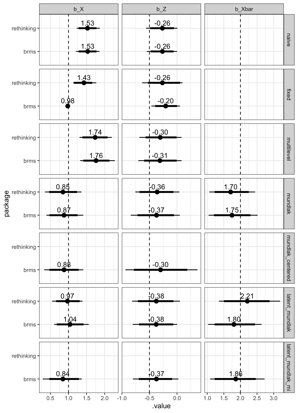
Figure 1: Estimated coefficients and the true values (dashed line)
For some reason, I did not manage to specify a uniform prior in rethinking. I think this explains the poor showing for the rethinking fixed effects model. Fixed effects regression + Bayes is not really a happy couple.
Gaussian simulations
Then, I simulated a Gaussian outcome instead. I didn’t run the rethinking models here, except for the latent Mundlak model.
Show code
set.seed(201910)
# families
N_groups <- 300
a0 <- (-2)
b_X <- (1)
b_Z <- (-0.5)
b_Ug <- (3)
# 2 or more siblings
g_sizes <- 2 + rpois(N_groups, lambda = 0.2) # sample into groups
table(g_sizes)
N_id <- sum(g_sizes)
g <- rep(1:N_groups, times = g_sizes)
Ug <- rnorm(N_groups, sd = 0.8) # group confounds
X <- rnorm(N_id, Ug[g] ) # individual varying trait
Z <- rnorm(N_groups) # group varying trait (observed)
Y <- a0 + b_X * X + b_Ug*Ug[g] + b_Z*Z[g] + rnorm(N_id)

groups <- tibble(id = factor(1:N_groups), Ug, Z)
sim <- tibble(id = factor(g), X, Y) %>% full_join(groups, by = "id") %>% arrange(id) %>% group_by(id) %>%
  mutate(Xbar = mean(X)) %>% ungroup()
sim %>% distinct(id, Ug, Xbar) %>% select(-id) %>% cor(use = "p")
lm(Y ~ X + Z, data = sim)
lm(Y ~ Ug + X + Z, data = sim)
lm(Y ~ id + X + Z, data = sim)

sim <- sim %>% group_by(id) %>%
  mutate(Xse = sd(X)/sqrt(n())) %>% ungroup() %>%
  mutate(X2 = X)
Implementations of the various models
Naive
brms
Show code
b_mn <- brm(Y ~ X + Z, data = sim,
            prior = c(
              set_prior("normal(0, 1)", class = "b", coef = "X"),
              set_prior("normal(0, 1)", class = "b", coef = "Z"),
              set_prior("normal(0, 2)", class = "Intercept")))
b_mn

b_mn %>% gather_draws(b_X, b_Z) %>% mean_hdci()
Fixed effects
brms
Show code
b_mf <- brm(Y ~ 1 + id + X + Z, data = sim,
            prior = c(
              set_prior("normal(0, 1)", class = "b", coef = "X"),
              set_prior("normal(0, 1)", class = "b", coef = "Z"),
              set_prior("normal(0, 2)", class = "b"))
            # , sample_prior = "only"
            )

# b_mf %>% gather_draws(`b_id.*`, regex=T) %>%
#   ggplot(aes(inv_logit(.value))) + geom_histogram(binwidth = .01)
b_mf %>% gather_draws(b_X, b_Z) %>% mean_hdci()
Multilevel
brms
Show code
b_mr <- brm(Y ~ (1|id) + X + Z, data = sim,
            prior = c(
              set_prior("normal(0, 1)", class = "b", coef = "X"),
              set_prior("normal(0, 1)", class = "b", coef = "Z"),
              set_prior("exponential(1)", class = "sd")))
b_mr

b_mr %>% gather_draws(b_X, b_Z) %>% mean_hdci()
Multilevel Mundlak
brms
Show code
b_mrx <- brm(Y ~ (1|id) + X + Z + Xbar, data = sim,
            prior = c(
              set_prior("normal(0, 1)", class = "b", coef = "X"),
              set_prior("normal(0, 1)", class = "b", coef = "Z"),
              set_prior("normal(0, 1)", class = "b", coef = "Xbar"),
              set_prior("exponential(1)", class = "sd")))
b_mrx

b_mrx %>% gather_draws(b_X, b_Z) %>% mean_hdci()
subtracting the group mean instead of adjusting for it
Show code
b_mrc <- brm(Y ~ (1|id) + X + Z, data = sim %>% mutate(X = X - Xbar),
            prior = c(
              set_prior("normal(0, 1)", class = "b", coef = "X"),
              set_prior("normal(0, 1)", class = "b", coef = "Z"),
              set_prior("exponential(1)", class = "sd")))
b_mrc

b_mrc %>% gather_draws(b_X, b_Z) %>% mean_hdci()
Multilevel Latent Mundlak
rethinking
Show code
dat <-  list(Y = Y, X = X, g = g, Ng = N_groups, Z = Z)
# The Latent Mundlak Machine
mru <- ulam(
  alist(
    # y model
    Y ~ normal(muY, sigmaY),
    muY <- a[g] + b_X*X + b_Z*Z[g] + buy*u[g],
    transpars> vector[Ng]:a <<- abar + z*tau,
    # X model
    X ~ normal(mu,sigma),
    mu <- aX + bux*u[g],
    vector[Ng]:u ~ normal (0,1),

    # priors
    z[g] ~ dnorm(0,1),
    c(aX, b_X, buy, b_Z) ~ dnorm(0, 1),
    bux ~ dexp(1),
    abar ~ dnorm (0,1),
    tau ~ dexp(1),
    c(sigma, sigmaY) ~ dexp(1)
  ),iter = 2000,
  data = dat, chains = 4, cores=4, sample=TRUE)

mru %>% gather_draws(b_X, b_Z) %>% mean_hdci()
brms
brms me() measurement error notation
Show code
b_mru_gr <- brm(Y ~ 1 +(1|id) + X + Z + me(Xbar, Xse, gr = id), data = sim,
             prior = c(
                 set_prior("normal(0, 1)", class = "b", coef = "X"),
                 set_prior("normal(0, 1)", class = "b", coef = "Z"),
                 set_prior("normal(0, 1)", class = "b", coef = "meXbarXsegrEQid"),
                 set_prior("exponential(1)", class = "sd"),
                 set_prior("exponential(1)", class = "sdme")))
brms mi() missingness notation
Show code
b_mru_mi <- brm(bf(Y ~ (1|id) + X + Z + mi(X2)) +
             bf(X2 | mi(Xse) ~ (1|id), family = gaussian()), data = sim %>% mutate(X2 = X),
            prior = c(
              set_prior("normal(0, 1)", class = "b", coef = "X", resp = "Y"),
              set_prior("normal(0, 1)", class = "b", coef = "Z", resp = "Y"),
              set_prior("normal(0, 1)", class = "b", coef = "miX2", resp = "Y"),
              set_prior("exponential(1)", class = "sd", resp = "Y"),
              set_prior("exponential(1)", class = "sd", resp = "X2"),
              set_prior("exponential(1)", class = "sigma", resp = "X2")))
b_mru_mi

b_mru_mi %>% gather_draws(b_Y_X, b_Y_Z) %>% mean_hdci()
working implementation of the mi model using nonlinear syntax
Show code
latent_formula <- bf(nl = TRUE,
  # Y model
  Y ~ interceptY  + bX*X + X2l + bZ*Z,
  X2l ~ 0 + mi(X2),
  interceptY ~ 1 + (1 | id),
  bX + bZ ~ 1, family = gaussian()) +
  bf(X2 | mi(Xse) ~ 1 + (1|id), family = gaussian()) #+
#  bernoulli()

# get_prior(latent_formula, data = sim)

b_mru_minl <- brm(latent_formula, data = sim,
            prior = c(
              set_prior("normal(0, 1)", class = "b", nlpar = "X2l", resp = "Y"),
              set_prior("normal(0, 1)", class = "b", nlpar = "bX", resp = "Y"),
              set_prior("normal(0, 1)", class = "b", nlpar = "bZ", resp = "Y"),
              # set_prior("normal(0, 1)", class = "b", nlpar = "bX2", resp = "Y"),
              set_prior("normal(0, 1)", class = "b", nlpar = "interceptY", resp = "Y"),
              set_prior("exponential(1)", class = "sd", nlpar = "interceptY", resp = "Y"),
              set_prior("normal(0, 1)", class = "Intercept", resp = "X2"),
              set_prior("exponential(1)", class = "sd", resp = "X2")))
b_mru_minl
non-working implementation of Matti Vuorre’s approach
This is the approach Matti Vuorre posted on his blog, except that I rearranged to instead the slope of Xbar. This approach does not work at all, as far as I can tell.
Show code
latent_formula <- bf(
  # Y model
  Y ~ interceptY  + bX*X + bXbar*Xbar + bZ*Z,
  interceptY ~ 1 + (1 | id),
  bX + bZ + bXbar ~ 1,

  # Xbar model
  nlf(X ~ Xbar),
  Xbar ~ 1 + (1 | id),
  nl = TRUE
) #+
#  bernoulli()

get_prior(latent_formula, data = sim)

b_mru_mv <- brm(latent_formula, data = sim,
            prior = c(
              set_prior("normal(0, 1)", class = "b", nlpar = "bX"),
              set_prior("normal(0, 1)", class = "b", nlpar = "bZ"),
              set_prior("normal(0, 1)", class = "b", nlpar = "bXbar"),
              set_prior("normal(0, 1)", class = "b", nlpar = "Xbar"),
              set_prior("normal(0, 1)", class = "b", nlpar = "interceptY"),
              set_prior("exponential(1)", class = "sd", nlpar = "interceptY"),
              set_prior("exponential(1)", class = "sd", nlpar = "Xbar")))
Show code
b_mru_mv Family: gaussian
Links: mu = identity; sigma = identity
Formula: Y ~ interceptY + bX * X + bXbar * Xbar + bZ * Z
interceptY ~ 1 + (1 | id)
bX ~ 1
bZ ~ 1
bXbar ~ 1
X ~ Xbar
Xbar ~ 1 + (1 | id)
Data: sim (Number of observations: 646)
Draws: 4 chains, each with iter = 2000; warmup = 1000; thin = 1;
total post-warmup draws = 4000
Group-Level Effects:
~id (Number of levels: 300)
Estimate Est.Error l-95% CI u-95% CI Rhat
sd(interceptY_Intercept) 1.76 1.19 0.06 3.43 1.35
sd(Xbar_Intercept) 1.54 0.99 0.03 3.67 1.19
Bulk_ESS Tail_ESS
sd(interceptY_Intercept) 10 88
sd(Xbar_Intercept) 16 84
Population-Level Effects:
Estimate Est.Error l-95% CI u-95% CI Rhat
interceptY_Intercept -0.72 0.92 -2.25 1.14 1.03
bX_Intercept 0.11 1.10 -2.08 2.16 1.24
bZ_Intercept -0.41 0.18 -0.75 -0.04 1.01
bXbar_Intercept 0.11 1.08 -1.98 2.13 1.24
Xbar_Intercept 0.06 1.17 -1.80 3.70 1.19
Bulk_ESS Tail_ESS
interceptY_Intercept 190 554
bX_Intercept 12 140
bZ_Intercept 1252 1963
bXbar_Intercept 12 136
Xbar_Intercept 15 51
Family Specific Parameters:
Estimate Est.Error l-95% CI u-95% CI Rhat Bulk_ESS Tail_ESS
sigma 1.47 0.06 1.37 1.59 1.02 257 96
Draws were sampled using sampling(NUTS). For each parameter, Bulk_ESS
and Tail_ESS are effective sample size measures, and Rhat is the potential
scale reduction factor on split chains (at convergence, Rhat = 1).Summary
Show code
draws <- bind_rows(
  brms_naive = b_mn %>% gather_draws(b_X, b_Z),
  brms_fixed = b_mf %>% gather_draws(b_X, b_Z),
  brms_multilevel = b_mr %>% gather_draws(b_X, b_Z),
  brms_mundlak = b_mrx %>% gather_draws(b_X, b_Z, b_Xbar),
  brms_mundlak_centered = b_mrc %>% gather_draws(b_X, b_Z),
  rethinking_latent_mundlak = mru %>% gather_draws(b_X, b_Z, buy),
  brms_latent_mundlak = b_mru_gr %>% gather_draws(b_X, b_Z, bsp_meXbarXsegrEQid),
  brms_latent_mundlak_mi = b_mru_mi %>% gather_draws(b_Y_X, b_Y_Z, bsp_Y_miX2),
 .id = "model") %>%
  separate(model, c("package", "model"), extra = "merge") %>%
  mutate(model = fct_inorder(factor(model)),
         .variable = str_replace(.variable, "_Y", ""),
         .variable = recode(.variable,
                            "buy" = "b_Xbar",
                            "bsp_miX2" = "b_Xbar",
                            "bsp_meXbarXsegrEQid" = "b_Xbar"),
         .variable = factor(.variable, levels = c("b_X", "b_Z", "b_Xbar")))

draws <- draws %>% group_by(package, model, .variable) %>%
  mean_hdci(.width = c(.95, .99)) %>%
  ungroup()

ggplot(draws, aes(y = package, x = .value, xmin = .lower, xmax = .upper)) +
  geom_pointinterval(position = position_dodge(width = .4)) +
  ggrepel::geom_text_repel(aes(label = if_else(.width == .95, sprintf("%.2f", .value), NA_character_)), nudge_y = .1) +
  geom_vline(aes(xintercept = true_val), linetype = 'dashed', data = tibble(true_val = c(b_X, b_Z, b_Ug - b_X), .variable = factor(c("b_X", "b_Z", "b_Xbar"), levels = c("b_X", "b_Z", "b_Xbar")))) +  scale_color_discrete(breaks = rev(levels(draws$model))) +
  facet_grid(model ~ .variable, scales = "free_x") +
  theme_bw() +
  theme(legend.position = c(0.99,0.99),
        legend.justification = c(1,1))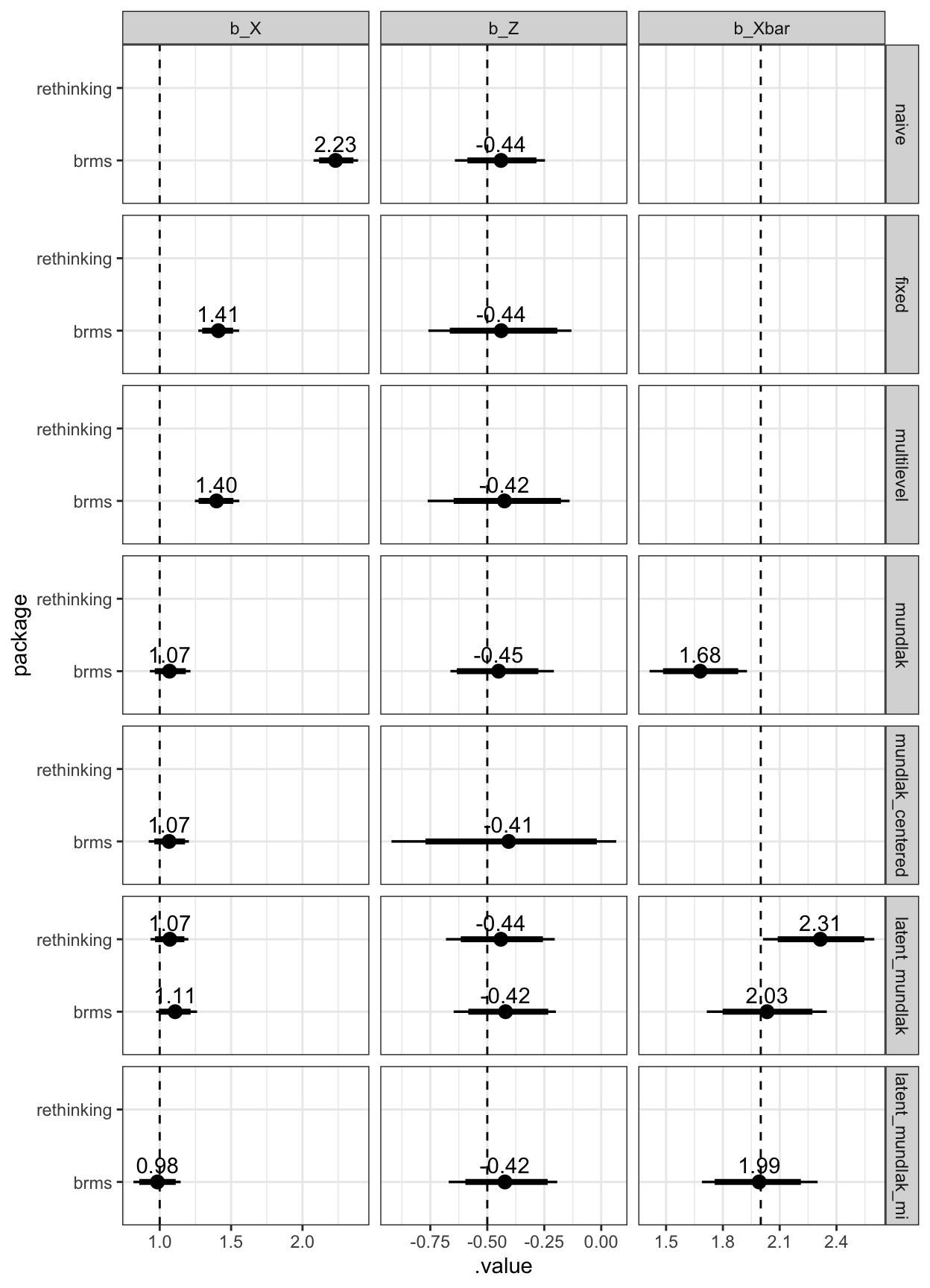
Figure 2: Estimated coefficients and the true values (dashed line)
Gaussian + binary exposure simulations
Finally, I simulated a Gaussian outcome and a binary exposure (X). Especially in small groups, the group average of a binary variable can be pretty far off. I didn’t run the rethinking models here, except for the latent Mundlak model.
I was not able to implement this model in brms. brms does not permit the specification of a binary variable as missing using mi(). And adjusting for Xbar using a linear probability model did not work.
Show code
set.seed(201910)
# families
N_groups <- 300
a0 <- (-2)
b_X <- (1)
b_Z <- (-0.5)
b_Ug <- (3)
# 2 or more siblings
g_sizes <- 2 + rpois(N_groups, lambda = 0.2) # sample into groups
table(g_sizes)
N_id <- sum(g_sizes)
g <- rep(1:N_groups, times = g_sizes)
Ug <- rnorm(N_groups, sd = 0.8) # group confounds
X <- rbern(N_id, p=inv_logit(rnorm(N_id, Ug[g] ) ) )   # individual varying trait
table(X)

Z <- rnorm(N_groups) # group varying trait (observed)
Y <- a0 + b_X * X + b_Ug*Ug[g] + b_Z*Z[g] + rnorm(N_id)

groups <- tibble(id = factor(1:N_groups), Ug, Z)
sim <- tibble(id = factor(g), X, Y) %>% full_join(groups, by = "id") %>% arrange(id) %>% group_by(id) %>%
  mutate(Xbar = mean(X)) %>% ungroup()
sim %>% distinct(id, Ug, Xbar) %>% select(-id) %>% cor(use = "p")
lm(Y ~ X + Z, data = sim)
lm(Y ~ Ug + X + Z, data = sim)
lm(Y ~ id + X + Z, data = sim)

sim <- sim %>% group_by(id) %>%
  mutate(Xse = sd(X)/sqrt(n())) %>% ungroup() %>%
  mutate(X2 = X)
Implementations of the various models
Naive
brms
Show code
b_mn <- brm(Y ~ X + Z, data = sim,
            prior = c(
              set_prior("normal(0, 1)", class = "b", coef = "X"),
              set_prior("normal(0, 1)", class = "b", coef = "Z"),
              set_prior("normal(0, 2)", class = "Intercept")))
b_mn

b_mn %>% gather_draws(b_X, b_Z) %>% mean_hdci()
Fixed effects
brms
Show code
b_mf <- brm(Y ~ 1 + id + X + Z, data = sim,
            prior = c(
              set_prior("normal(0, 1)", class = "b", coef = "X"),
              set_prior("normal(0, 1)", class = "b", coef = "Z"),
              set_prior("normal(0, 2)", class = "b"))
            # , sample_prior = "only"
            )

# b_mf %>% gather_draws(`b_id.*`, regex=T) %>%
#   ggplot(aes(inv_logit(.value))) + geom_histogram(binwidth = .01)
b_mf %>% gather_draws(b_X, b_Z) %>% mean_hdci()
Multilevel
brms
Show code
b_mr <- brm(Y ~ (1|id) + X + Z, data = sim,
            prior = c(
              set_prior("normal(0, 1)", class = "b", coef = "X"),
              set_prior("normal(0, 1)", class = "b", coef = "Z"),
              set_prior("exponential(1)", class = "sd")))
b_mr

b_mr %>% gather_draws(b_X, b_Z) %>% mean_hdci()
Multilevel Mundlak
brms
Show code
b_mrx <- brm(Y ~ (1|id) + X + Z + Xbar, data = sim,
            prior = c(
              set_prior("normal(0, 1)", class = "b", coef = "X"),
              set_prior("normal(0, 1)", class = "b", coef = "Z"),
              set_prior("normal(0, 1)", class = "b", coef = "Xbar"),
              set_prior("exponential(1)", class = "sd")))
b_mrx

b_mrx %>% gather_draws(b_X, b_Z) %>% mean_hdci()
subtracting the group mean instead of adjusting for it
Show code
b_mrc <- brm(Y ~ (1|id) + X + Z, data = sim %>% mutate(X = X - Xbar),
            prior = c(
              set_prior("normal(0, 1)", class = "b", coef = "X"),
              set_prior("normal(0, 1)", class = "b", coef = "Z"),
              set_prior("exponential(1)", class = "sd")))
b_mrc

b_mrc %>% gather_draws(b_X, b_Z) %>% mean_hdci()
Multilevel Latent Mundlak
rethinking
Show code
dat <-  list(Y = Y, X = X, g = g, Ng = N_groups, Z = Z)
# The Latent Mundlak Machine
mru <- ulam(
  alist(
    # y model
    Y ~ normal(muY, sigmaY),
    muY <- a[g] + b_X*X + b_Z*Z[g] + buy*u[g],
    transpars> vector[Ng]:a <<- abar + z*tau,
    # X model
    X ~ bernoulli(p),
    logit(p) <- aX + bux*u[g],
    vector[Ng]:u ~ normal (0,1),

    # priors
    z[g] ~ dnorm(0,1),
    c(aX, b_X, buy, b_Z) ~ dnorm(0, 1),
    bux ~ dexp(1),
    abar ~ dnorm (0,1),
    tau ~ dexp(1),
    c(sigma, sigmaY) ~ dexp(1)
  ),
  data = dat, chains = 4, cores=4, sample=TRUE)

mru %>% gather_draws(b_X, b_Z) %>% mean_hdci()
brms
brms me() measurement error notation
I had to add .01 to the Xse because brms does not permit 0 measurement error (when modelling measurement error).
Show code
b_mru_gr <- brm(Y ~ 1 +(1|id) + X + Z + me(Xbar, Xse, gr = id), data = sim %>% mutate(Xse = Xse + 0.01),
             prior = c(
                 set_prior("normal(0, 1)", class = "b", coef = "X"),
                 set_prior("normal(0, 1)", class = "b", coef = "Z"),
                 set_prior("normal(0, 1)", class = "b", coef = "meXbarXsegrEQid"),
                 set_prior("exponential(1)", class = "sd"),
                 set_prior("exponential(1)", class = "sdme")))
brms mi() missingness notation
brms does not support the mi() notation for binary variables. Also, it does not accept zero measurement error, so I averaged across groups to take the mean Xse.
Show code
b_mru_mi <- brm(bf(Y ~ (1|id) + X + Z + mi(X2)) +
             bf(X2 | mi(Xse) ~ (1|id)), family = gaussian(), data = sim %>% mutate(Xse = Xse + 0.01), iter = 4000,
            prior = c(
              set_prior("normal(0, 1)", class = "b", coef = "X", resp = "Y"),
              set_prior("normal(0, 1)", class = "b", coef = "Z", resp = "Y"),
              set_prior("normal(0, 1)", class = "b", coef = "miX2", resp = "Y"),
              set_prior("exponential(1)", class = "sd", resp = "Y"),
              set_prior("exponential(1)", class = "sd", resp = "X2"),
              set_prior("constant(0.01)", class = "sigma", resp = "X2")))
b_mru_mi

b_mru_mi %>% gather_draws(b_Y_X, b_Y_Z) %>% mean_hdci()
Summary
Show code
draws <- bind_rows(
  brms_naive = b_mn %>% gather_draws(b_X, b_Z),
  brms_fixed = b_mf %>% gather_draws(b_X, b_Z),
  brms_multilevel = b_mr %>% gather_draws(b_X, b_Z),
  brms_mundlak = b_mrx %>% gather_draws(b_X, b_Z, b_Xbar),
  brms_mundlak_centered = b_mrc %>% gather_draws(b_X, b_Z),
  rethinking_latent_mundlak = mru %>% gather_draws(b_X, b_Z, buy),
  brms_latent_mundlak = b_mru_gr %>% gather_draws(b_X, b_Z, bsp_meXbarXsegrEQid),
  brms_latent_mundlak_mi = b_mru_mi %>% gather_draws(b_Y_X, b_Y_Z, bsp_Y_miX2),
 .id = "model") %>%
  separate(model, c("package", "model"), extra = "merge") %>%
  mutate(model = fct_inorder(factor(model)),
         .variable = str_replace(.variable, "_Y", ""),
         .variable = recode(.variable,
                            "buy" = "b_Xbar",
                            "bsp_miX2" = "b_Xbar",
                            "bsp_meXbarXsegrEQid" = "b_Xbar"),
         .variable = factor(.variable, levels = c("b_X", "b_Z", "b_Xbar")))

draws <- draws %>% group_by(package, model, .variable) %>%
  mean_hdci(.width = c(.95, .99)) %>%
  ungroup()

ggplot(draws, aes(y = package, x = .value, xmin = .lower, xmax = .upper)) +
  geom_pointinterval(position = position_dodge(width = .4)) +
  ggrepel::geom_text_repel(aes(label = if_else(.width == .95, sprintf("%.2f", .value), NA_character_)), nudge_y = .1) +
  geom_vline(aes(xintercept = true_val), linetype = 'dashed', data = tibble(true_val = c(b_X, b_Z, b_Ug - b_X), .variable = factor(c("b_X", "b_Z", "b_Xbar"), levels = c("b_X", "b_Z", "b_Xbar")))) +  scale_color_discrete(breaks = rev(levels(draws$model))) +
  facet_grid(model ~ .variable, scales = "free_x") +
  theme_bw() +
  theme(legend.position = c(0.99,0.99),
        legend.justification = c(1,1))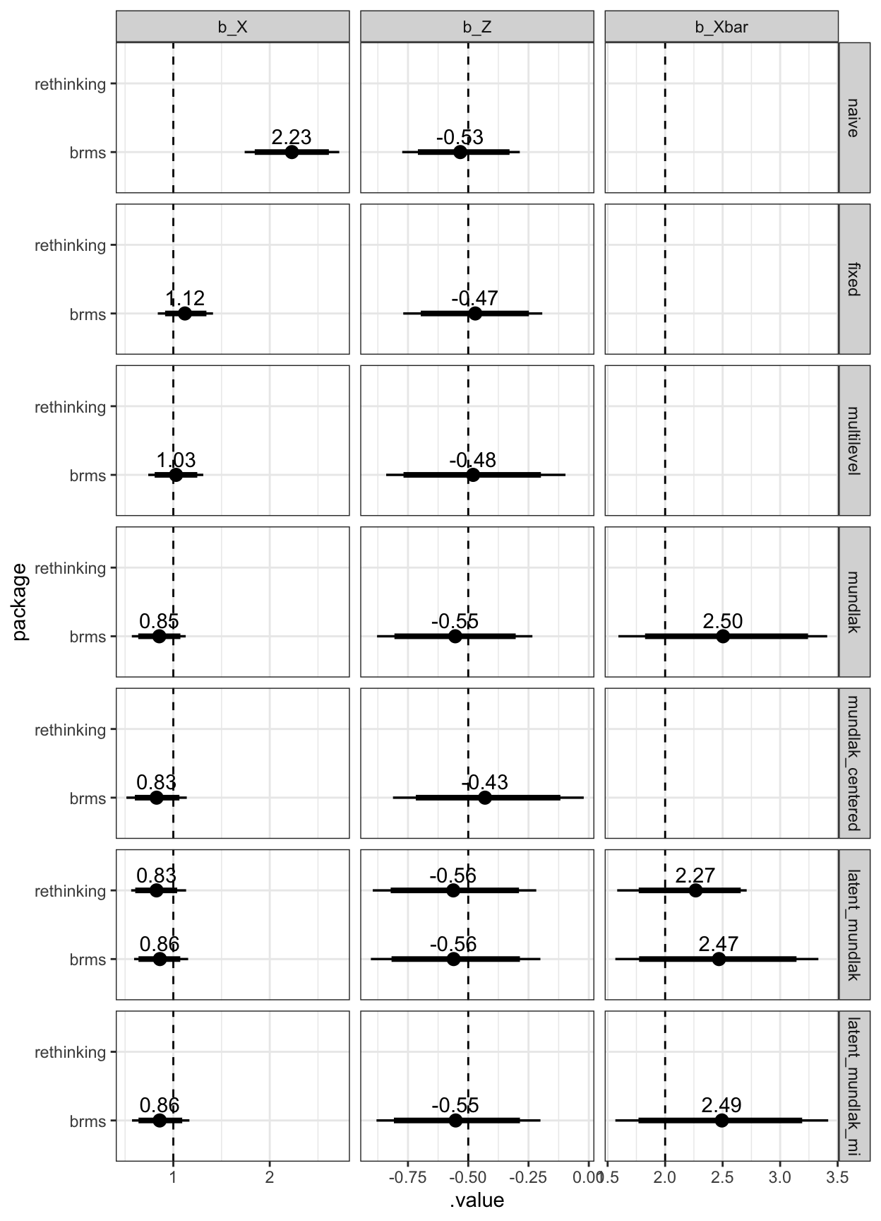
Figure 3: Estimated coefficients and the true values (dashed line)
the group here can be an individual measured several times, a sibling group, a school, a nation, etc.↩︎
Mundlak, Y. 1978: On the pooling of time series and cross section data. Econometrica 46:69-85.↩︎
What McElreath calls Full Luxury Bayes: Latent Mundlak machine↩︎
I think the reason he thought it works is that in the data he used, from McNeish & Hamaker 2020, the group mean varies very little except for measurement error, so we expect it not to make a difference.↩︎