Comparison of descriptives across populations

Loading details

source("0__helpers.R")
opts_chunk$set(render = pander_handler,warning=FALSE,cache=FALSE,tidy=FALSE,autodep=TRUE,dev='png',fig.width=12,fig.height=7.5)
load("rpqa.rdata")
load("ddb.rdata")
load("krmh.rdata")
load("swed1.rdata")
load("swed.rdata")
demo_mod_swed = aggDemoTrends(swed)
demo_old_swed = aggDemoTrends(ddb.1) %>% 
    mutate(Population = "Historical Sweden") %>%
    melt(id=c("Population","Year","Parent")) %>% 
    group_by(Population,Parent,variable) %>%
    summarise(value = mean(value,na.rm=T))
rm(rpqa,ddb, krmh, swed)
desc_theme = theme_minimal(base_size = 24)
update_geom_defaults("bar",   list(fill = "#6c92b2", alpha = 1/2))

mymin = theme_minimal(base_size = 20) +theme(panel.grid.major.y =element_blank(),panel.grid.major.x = element_line(colour="#eeeeee"))

rpqa.1$Population = "Québec"
ddb.1$Population = "Historical Sweden"
krmh.1$Population = "Krummhörn"
swed.1$Population = "20th-century Sweden"
all = rbind(
    rpqa.1 %>% select(paternalage, maternalage, age_at_1st_child, age_at_last_child, children, male, Population, survive1y,surviveR, ever_married),
    ddb.1 %>% select(paternalage, maternalage, age_at_1st_child, age_at_last_child, children, male, Population, survive1y,surviveR, ever_married),
    krmh.1 %>% select(paternalage, maternalage, age_at_1st_child, age_at_last_child, children, male, Population, survive1y,surviveR, ever_married),
    swed.1 %>% select(paternalage, maternalage, age_at_1st_child, age_at_last_child, children, male, Population, survive1y,surviveR, ever_married)
)
rm(rpqa.1,ddb.1, krmh.1,swed.1)
all = data.table(all)

all[, paternalage := 10 * paternalage]
all[, maternalage := 10 * maternalage]
all[, age_at_1st_child := 10 * age_at_1st_child]
all[, age_at_last_child := 10 * age_at_last_child]

mean_sd = function(x) { paste0(round(mean(x, na.rm=T),2), " (",round(sd(x,na.rm=T),2),")") }
mean_sd_bin = function(x) { 
    m= mean(x, na.rm=T)
    sprintf("%.3f (%.3f)",m,m*(1-m))
}
nodot = function(x) { 
    names(x) = stringr::str_replace_all(names(x),stringr::fixed(".")," ")
    x
}
all[, sex := factor(ifelse(male==1,"male","female"))]
all[, reproductive_timespan := age_at_last_child - age_at_1st_child]
all = all[!is.na(sex), ]
all = data.frame(all)

Reproductive timing

demo_mod_swed$Population = "20th-century Sweden"
demo_mod_swed$lty = factor("all", levels = c("first","all","last"))

rep_timing_comp = ggplot(data = demo_mod_swed) + 
    geom_line(aes(x= Year, y = first, colour = Population, linetype = "first"), colour = "#8A846C", size = 1) + 
  geom_line(aes(x = Year, y = all, colour = Population, linetype = "all"), size = 1) +
    geom_line(aes(x= Year, y = last, colour = Population,linetype = "last"), colour = "#8A846C", size = 1) + 
    geom_hline(aes(yintercept = value, colour = Population,linetype = variable), data = demo_old_swed, size = 1) +
    geom_text(aes(x = 1980 + ifelse(variable == "all", 0, ifelse(variable == "first", -33, 0)), 
                                y = value + 0.3, colour = Population, 
                                label = paste(variable,"births in Sweden 1737-1880")), data = demo_old_swed) + 
    pop_colour + 
    scale_linetype_manual("Birth", breaks = c("last", "all","first"), values = c( "solid","dashed", "dotted")) +
        geom_text(aes(x = Year, y = all + 0.3, 
                                    label = ifelse(Year > 1670 & Year %% 15 == 0, round(all), NA))) + 
    facet_wrap(~ Parent,scales = "free_y") +
    desc_theme + 
    scale_y_continuous("Parental age at birth", limits = c(23,40)) + 
    theme(legend.position = c(1,1),
  legend.justification = c(1,1), 
  legend.box = "horizontal",
  panel.margin = unit(2, "lines"))
rep_timing_comp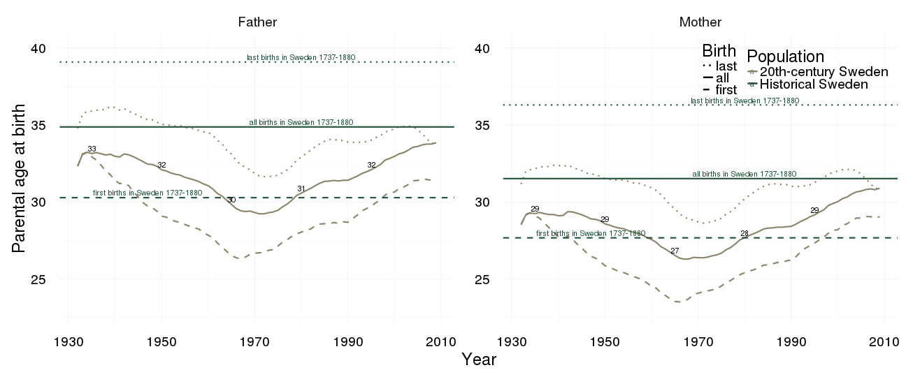

plot of chunk unnamed-chunk-1

Age at first child

all %>% 
    group_by(Population, sex) %>% 
    summarise(value = mean_sd(age_at_1st_child)) %>%
    dcast(formula = sex ~ Population) %>% na.omit()

sex	20th-century Sweden	Historical Sweden	Krummhörn	Québec
female	25.02 (5.09)	25.85 (4.84)	26.58 (4.44)	23.65 (4.87)
male	28.07 (5.6)	28.13 (5.18)	29.29 (5.36)	28.69 (6.01)

all %>% mutate(age_at_1st_child = ifelse(Population == "20th-century Sweden", age_at_1st_child + runif(n())-0.5, age_at_1st_child)) -> all # want smooth density even though we only have ages at year granularity

ggplot(all, aes(x = Population, y = age_at_1st_child, group = interaction(Population,sex))) + 
    coord_flip()+
    ylab("Age at first child") +
    geom_violin(aes(linetype = sex), position = position_dodge(width=1)) +
    geom_linerange(stat = "summary", fun.data="median_hilow", colour = "#aec05d", position = position_dodge(width=1)) +
    geom_pointrange(stat = "summary", fun.data="mean_cl_boot",colour = "#6c92b2", size = 1, position = position_dodge(width=1)) +
    mymin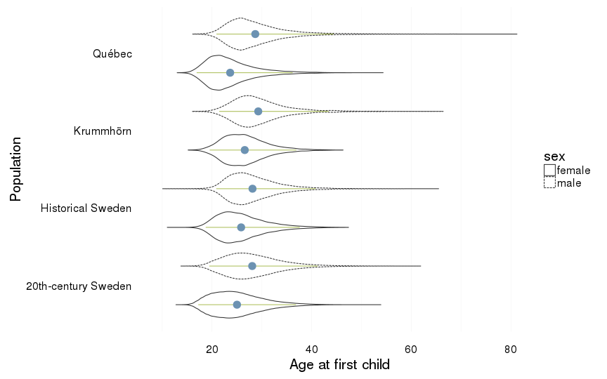

plot of chunk unnamed-chunk-2

ggplot(all, aes(x = age_at_1st_child, fill = Population)) +
    ylab("Density") +
    xlab("Age at first child") +
    facet_grid( sex ~ . )+
    geom_density(alpha = 0.5, position = position_identity(), colour = NA)+
    mymin +  pop_colour + pop_fill +
    theme(legend.position = c(1,1),
                legend.justification = c(1,1)) ->
    gg_age_at_1st_child
gg_age_at_1st_child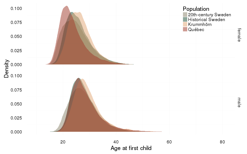

plot of chunk unnamed-chunk-2

Age at last child

all %>% 
    group_by(Population, sex) %>% 
    summarise(value = mean_sd(age_at_last_child)) %>%
    dcast(formula = sex ~ Population)

sex	20th-century Sweden	Historical Sweden	Krummhörn	Québec
female	30.34 (5.41)	34.79 (7.2)	35.95 (6.34)	37.27 (6.88)
male	33.57 (6.14)	37.52 (8.29)	39.61 (7.5)	43.9 (8.95)

all %>% mutate(age_at_last_child = ifelse(Population == "20th-century Sweden", age_at_last_child + runif(n())-0.5, age_at_last_child)) -> all # want smooth density even though we only have ages at year granularity

ggplot(all, aes(x = Population, y = age_at_last_child, group = interaction(Population,sex))) + 
    coord_flip()+
    ylab("Age at last child") +
    geom_violin(aes(linetype = sex), position = position_dodge(width=1)) +
    geom_linerange(stat = "summary", fun.data="median_hilow", colour = "#aec05d", position = position_dodge(width=1)) +
    geom_pointrange(stat = "summary", fun.data="mean_cl_boot",colour = "#6c92b2", size = 1, position = position_dodge(width=1)) +
    mymin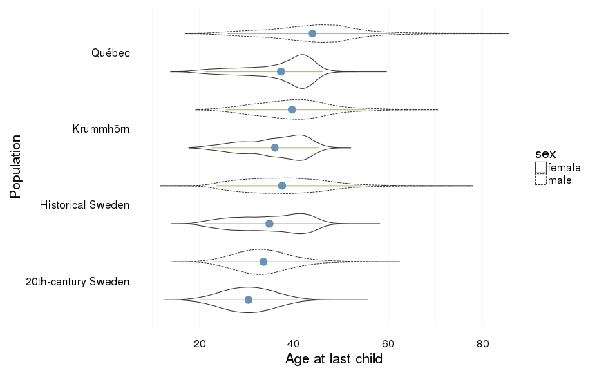

plot of chunk unnamed-chunk-3

ggplot(all, aes(x = age_at_last_child, fill = Population)) + 
    ylab("Density") +
    xlab("Age at last child") +
    facet_grid( sex ~ . )+
    geom_density(alpha = 0.5, position = position_identity(), colour = NA)+
    mymin + pop_colour + pop_fill +
    theme(legend.position = c(1,1),
                legend.justification = c(1,1)) ->
    gg_age_at_last_child
gg_age_at_last_child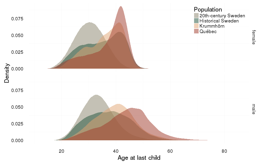

plot of chunk unnamed-chunk-3

Reproductive timespan

all %>% 
    group_by(Population, sex) %>% 
    summarise(value = mean_sd(reproductive_timespan)) %>%
    dcast(formula = sex ~ Population)

sex	20th-century Sweden	Historical Sweden	Krummhörn	Québec
female	5.32 (4.74)	8.94 (6.94)	9.37 (6.61)	13.62 (7.54)
male	5.5 (5.4)	9.39 (7.4)	10.32 (6.97)	15.21 (8.54)

all %>% mutate(reproductive_timespan = ifelse(Population == "20th-century Sweden", reproductive_timespan + runif(n())-0.5, reproductive_timespan)) -> all # want smooth density even though we only have ages at year granularity
all %>% mutate(reproductive_timespan = ifelse(reproductive_timespan<0,0,reproductive_timespan)) -> all

ggplot(all, aes(x = Population, y = reproductive_timespan, group = interaction(Population,sex))) +
    coord_flip()+
    ylab("Reproductive timespan") +
    geom_violin(aes(linetype = sex),position = position_dodge(width=1)) +
    geom_linerange(stat = "summary", fun.data="median_hilow", colour = "#aec05d", position = position_dodge(width=1)) +
    geom_pointrange(stat = "summary", fun.data="mean_cl_boot",colour = "#6c92b2", size = 1, position = position_dodge(width=1)) +
    mymin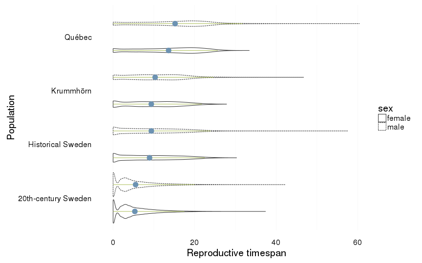

plot of chunk unnamed-chunk-4

ggplot(all, aes(x = reproductive_timespan, fill = Population)) + 
    ylab("Density") +
    xlab("Reproductive timespan") +
    facet_grid( sex ~ . )+
    geom_density(alpha = 0.5, position = position_identity(), colour = NA)+
    mymin + pop_colour + pop_fill +
    theme(legend.position = c(1,1),
                legend.justification = c(1,1))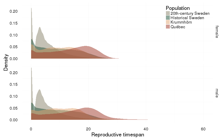

plot of chunk unnamed-chunk-4

Paternal age

all %>% 
    group_by(Population) %>% 
    summarise(value = mean_sd(paternalage)) %>%
    dcast(formula = . ~ Population)

.	20th-century Sweden	Historical Sweden	Krummhörn	Québec
.	31.84 (7.05)	34.37 (7.69)	35.23 (7.56)	36.33 (8.49)

all %>% mutate(paternalage = ifelse(Population == "20th-century Sweden", paternalage + runif(n())-0.5, paternalage)) -> all # want smooth density even though we only have ages at year granularity

ggplot(all, aes(x = Population, y = paternalage)) + 
    coord_flip()+
    ylab("Paternal age") +
    geom_violin() +
    geom_linerange(stat = "summary", fun.data="median_hilow", colour = "#aec05d", position = position_dodge(width=0.4)) +
    geom_pointrange(stat = "summary", fun.data="mean_cl_boot",colour = "#6c92b2", size = 1, position = position_dodge(width=0.4)) +
    mymin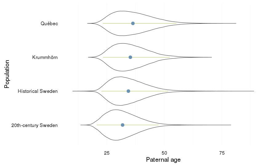

plot of chunk unnamed-chunk-5

ggplot(aes(x = paternalage), data = all) + 
    geom_histogram(binwidth=1) +
    xlab("Paternal age") +
    facet_wrap(~ Population, scale = "free_y") + 
    mymin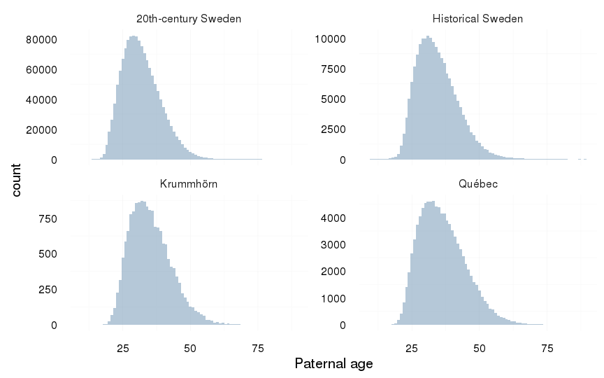

plot of chunk unnamed-chunk-5

ggplot(all, aes(x = paternalage, fill = Population)) + 
    ylab("Density") +
    xlab("Paternal age") +
    geom_density(alpha = 0.5, position = position_identity(), colour = NA)+
    mymin + pop_colour + pop_fill +
    theme(legend.position = c(1,1),
                legend.justification = c(1,1))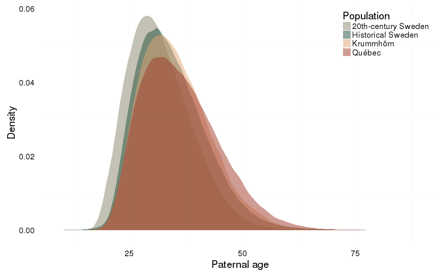

plot of chunk unnamed-chunk-5

Maternal age

all %>% 
    group_by(Population) %>% 
    summarise(value = mean_sd(maternalage)) %>%
    dcast(formula = . ~ Population)

.	20th-century Sweden	Historical Sweden	Krummhörn	Québec
.	28.34 (6.11)	31.54 (6.32)	31.53 (5.88)	29.57 (6.68)

all %>% mutate(maternalage = ifelse(Population == "20th-century Sweden", maternalage + runif(n())-0.5, maternalage)) -> all # want smooth density even though we only have ages at year granularity

ggplot(all, aes(x = Population, y = maternalage)) + 
    coord_flip()+
    ylab("Maternal age") +
    geom_violin() +
    geom_linerange(stat = "summary", fun.data="median_hilow", colour = "#aec05d", position = position_dodge(width=0.4)) +
    geom_pointrange(stat = "summary", fun.data="mean_cl_boot",colour = "#6c92b2", size = 1, position = position_dodge(width=0.4)) +
    mymin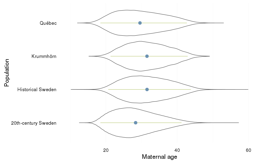

plot of chunk unnamed-chunk-6

ggplot(aes(x = maternalage), data = all) + 
    geom_histogram(binwidth=1) +
    xlab("Maternal age") +
    facet_wrap(~ Population, scale = "free_y") + 
    mymin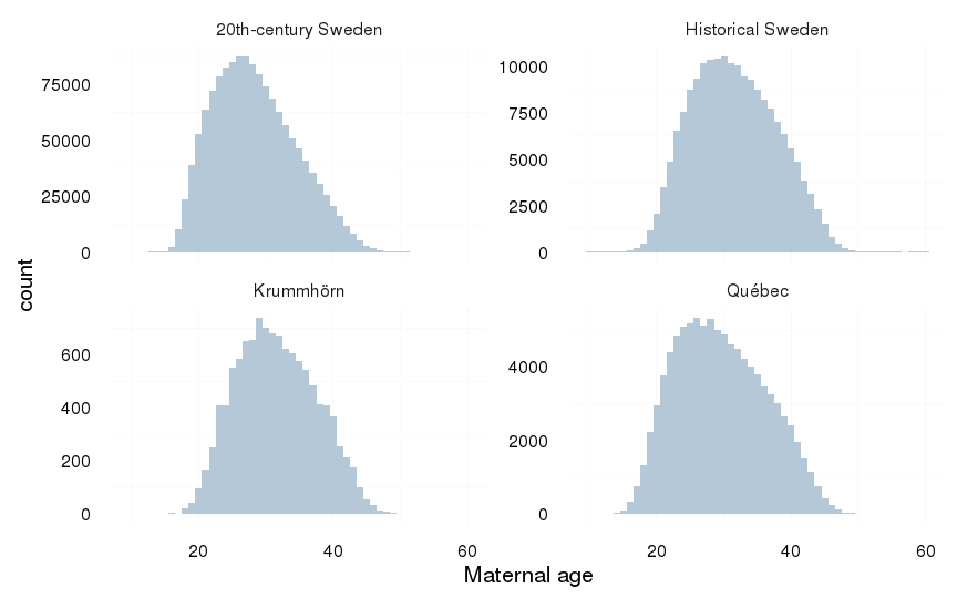

plot of chunk unnamed-chunk-6

ggplot(all, aes(x = maternalage, fill = Population)) + 
    ylab("Density") +
    xlab("Maternal age") +
    geom_density(alpha = 0.5, position = position_identity(), colour = NA)+
    mymin + pop_colour + pop_fill +
    theme(legend.position = c(1,1),
                legend.justification = c(1,1))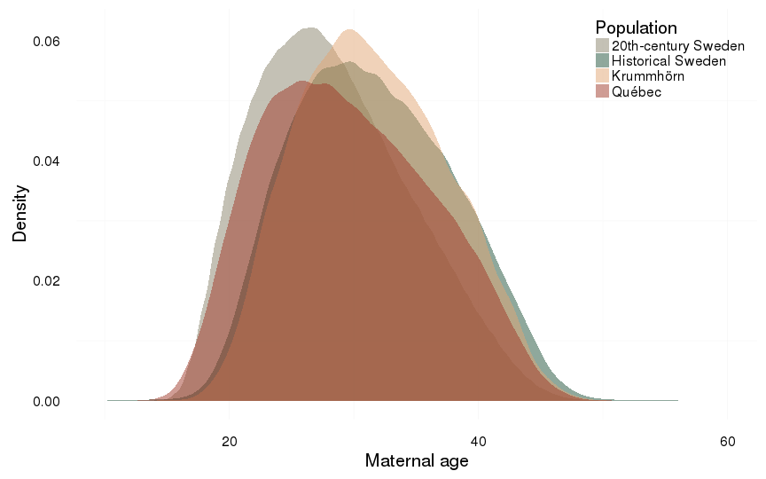

plot of chunk unnamed-chunk-6

Number of children

only those who married

all %>% 
    filter(ever_married == 1) %>%
    group_by(Population, sex) %>% 
    summarise(value = mean_sd(children)) %>%
    dcast(formula = sex ~ Population)

sex	20th-century Sweden	Historical Sweden	Krummhörn	Québec
female	2.15 (1.11)	3.66 (3.18)	3.66 (2.89)	7.3 (4.6)
male	2.17 (1.18)	4.04 (3.22)	4.09 (2.95)	8 (4.97)

all %>% 
    filter(ever_married == 1) %>%
ggplot(aes(x = Population, y = children, group = interaction(Population,sex))) +
    coord_flip()+
    geom_violin(aes(linetype = sex),position = position_dodge(width=1)) +
    geom_linerange(stat = "summary", fun.data="median_hilow", colour = "#aec05d", position = position_dodge(width=1)) +
    geom_pointrange(stat = "summary", fun.data="mean_cl_boot",colour = "#6c92b2", size = 1, position = position_dodge(width=1)) +
    mymin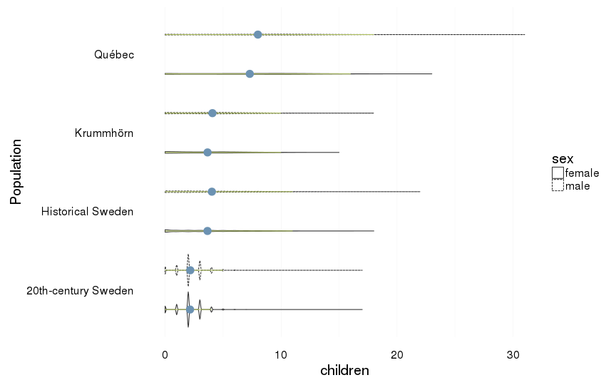

plot of chunk unnamed-chunk-7

all %>% 
    filter(ever_married == 1) %>%
ggplot(aes(x = children, y = ..density.., fill = Population)) + 
    geom_histogram(aes(y = ..density..), position = position_dodge(width = 1),binwidth=1.1) +
    scale_x_continuous(breaks = seq(0,25,by=2)) +
    mymin +
    theme(legend.position = c(1,1),
                legend.justification = c(1,1))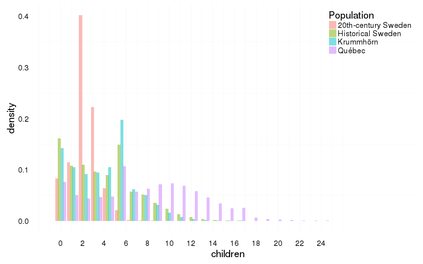

plot of chunk unnamed-chunk-7

all %>% 
    filter(ever_married == 1) %>%
ggplot(aes(x = children)) + 
    geom_histogram(binwidth=1) +
    facet_wrap(~ Population, scale = "free_y") + 
    mymin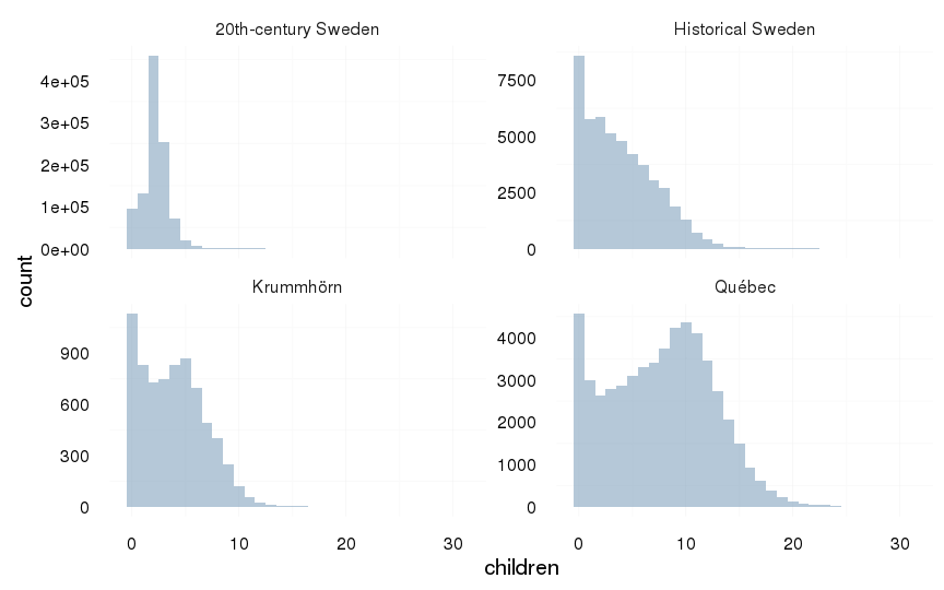

plot of chunk unnamed-chunk-7

only those who had children at all

all %>% 
    filter(children > 0) %>%
    group_by(Population, sex) %>% 
    summarise(value = mean_sd(children)) %>%
    dcast(formula = sex ~ Population)

sex	20th-century Sweden	Historical Sweden	Krummhörn	Québec
female	2.29 (0.95)	4.53 (2.9)	4.41 (2.6)	7.97 (4.2)
male	2.33 (1.01)	4.68 (3)	4.76 (2.63)	8.66 (4.58)

all %>% 
    filter(children > 0) %>%
ggplot(aes(x = Population, y = children, group = interaction(Population,sex))) +
    coord_flip()+
    geom_violin(aes(linetype = sex),position = position_dodge(width=1)) +
    geom_linerange(stat = "summary", fun.data="median_hilow", colour = "#aec05d", position = position_dodge(width=1)) +
    geom_pointrange(stat = "summary", fun.data="mean_cl_boot",colour = "#6c92b2", size = 1, position = position_dodge(width=1)) +
    mymin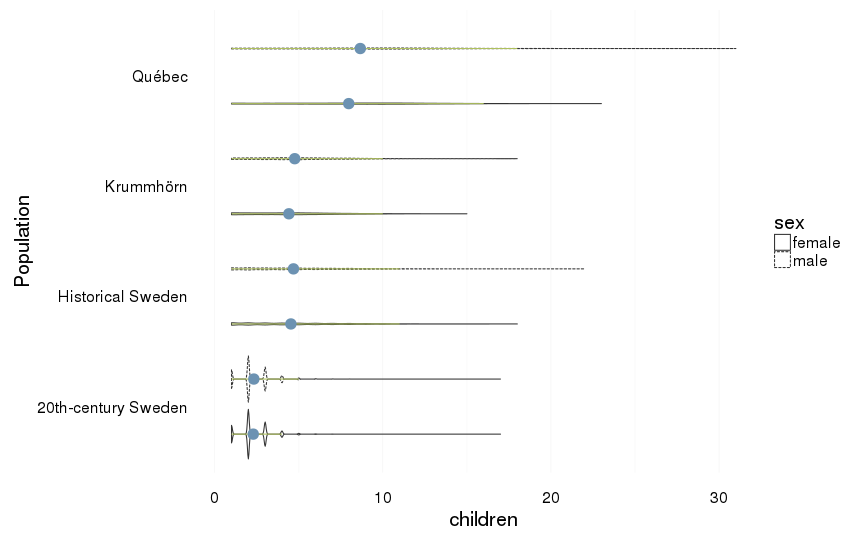

plot of chunk unnamed-chunk-8

all %>% 
    filter(children > 0) %>%
ggplot(aes(x = children, y = ..density.., fill = Population)) + 
    geom_histogram(aes(y = ..density..), position = position_dodge(width = 1),binwidth=1.1) +
    scale_x_continuous(breaks = seq(0,25,by=2)) +
    mymin +
    theme(legend.position = c(1,1),
                legend.justification = c(1,1))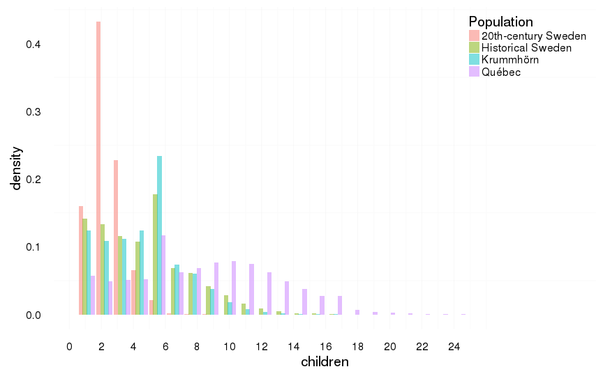

plot of chunk unnamed-chunk-8

all %>% 
    filter(children > 0) %>%
ggplot(aes(x = children)) + 
    geom_histogram(binwidth=1) +
    facet_wrap(~ Population, scale = "free_y") + 
    mymin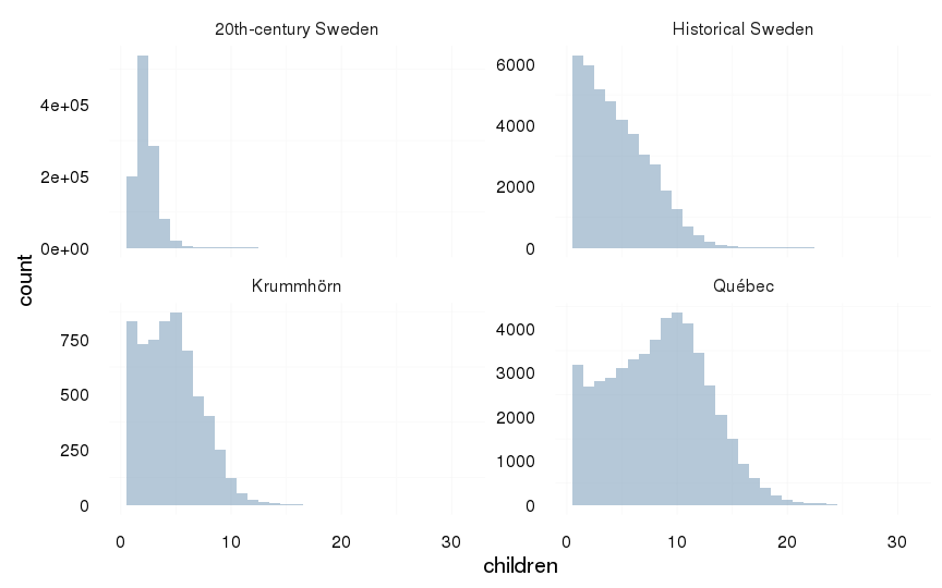

plot of chunk unnamed-chunk-8

all included, including those who died in childhood

all %>% 
    group_by(Population, sex) %>% 
    summarise(value = mean_sd(children)) %>%
    dcast(formula = sex ~ Population)

sex	20th-century Sweden	Historical Sweden	Krummhörn	Québec
female	1.91 (1.22)	1.04 (2.36)	1.78 (2.72)	3.93 (4.96)
male	1.79 (1.32)	0.96 (2.32)	1.62 (2.73)	3.68 (5.22)

all %>% 
ggplot(aes(x = Population, y = children, group = interaction(Population,sex))) +
    coord_flip()+
    geom_violin(aes(linetype = sex),position = position_dodge(width=1)) +
    geom_linerange(stat = "summary", fun.data="median_hilow", colour = "#aec05d", position = position_dodge(width=1)) +
    geom_pointrange(stat = "summary", fun.data="mean_cl_boot",colour = "#6c92b2", size = 1, position = position_dodge(width=1)) +
    mymin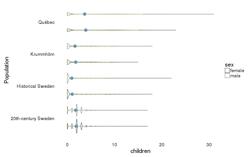

plot of chunk unnamed-chunk-9

ggplot(all, aes(x = children, y = ..density.., fill = Population)) + 
    geom_histogram(aes(y = ..density..), position = position_dodge(width = 1),binwidth=1.1) +
    mymin +
    theme(legend.position = c(1,1),
                legend.justification = c(1,1))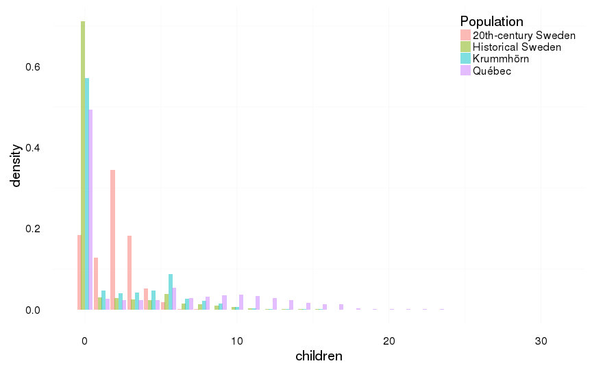

plot of chunk unnamed-chunk-9

ggplot(aes(x = children), data = all) + 
    geom_histogram(binwidth=1) +
    facet_wrap(~ Population, scale = "free_y") + 
    mymin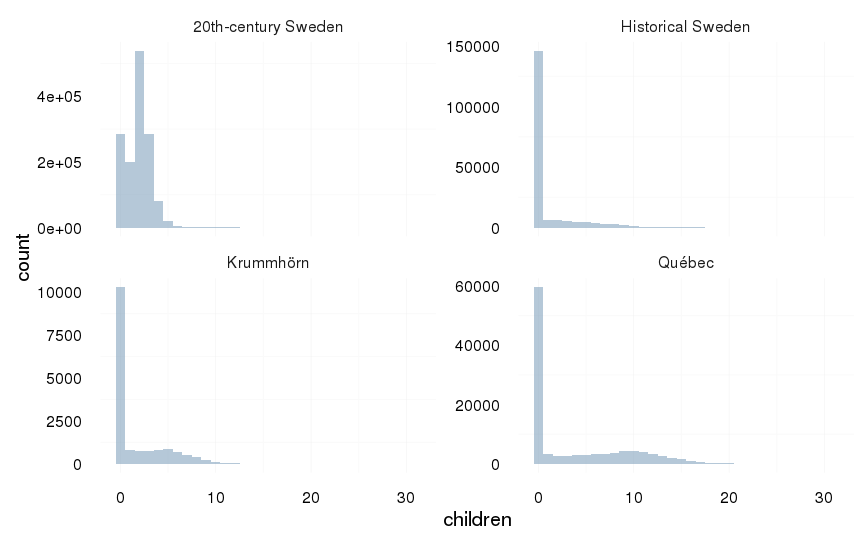

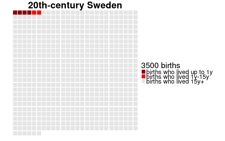
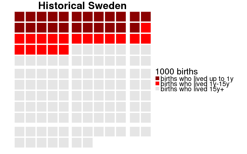
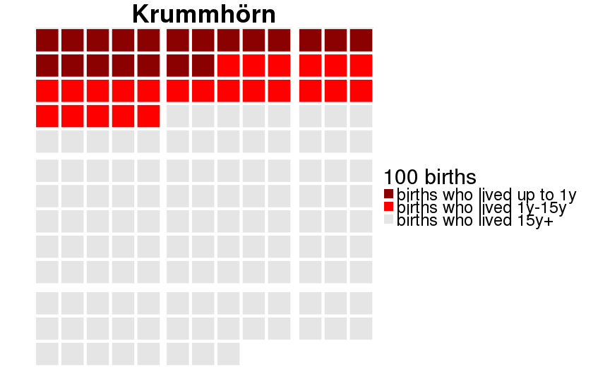
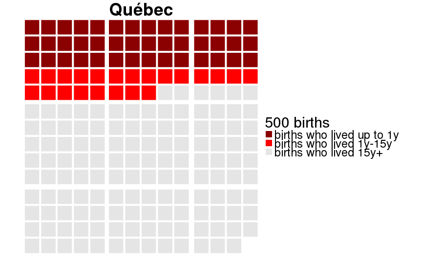
plot of chunk unnamed-chunk-9

Child mortality

number of children surviving their first year

opts_chunk$set(message=FALSE,warning=FALSE)
load("swed2.rdata")
swed.2$Population = "20th-century Sweden"
all = data.table(all)
all = rbind(
    all[Population != "20th-century Sweden", list(paternalage, maternalage, age_at_1st_child, age_at_last_child, children, male, Population, survive1y,surviveR)],
    swed.2[byear < 1990, list(paternalage, maternalage, age_at_1st_child, age_at_last_child, children, male, Population, survive1y,surviveR)]
)
rm(swed.2)
all = setDF(all)
all$sex = factor(ifelse(all$male==1,"male","female"))
all$reproductive_timespan = all$age_at_last_child  - all$age_at_1st_child
all$`Birth outcome` = 1+all$survive1y+all$surviveR
all = all[!is.na(all$sex), ]

library(formr)
in_100 = function(x) {
    x = na.omit(x)
    prop = round(mean(x) * 100)
    c(rep("lived to 1 year", prop), rep("died", 100-prop))
}
counts_unit = function(x, unit = 1000) {
    x = na.omit(x)
    bigger_units = round(table(x)/unit)
    bins = paste(unit,names(bigger_units))
    factor(rep(bins,bigger_units), levels = bins)
}
qwaffle = function(Pop, unit = 1000) {
    all %>% 
        filter(Population == Pop) %>% 
        .[, "Birth outcome"] %>%
        counts_unit(., unit) %>% 
        qplot_waffle_tile() + 
            theme(text = element_text(size = 30)) + 
            scale_fill_manual(paste(unit, "births"),breaks=1:3,labels=c("births who lived up to 1y","births who lived 1y-15y","births who lived 15y+"), values=c("darkred","red","gray90")) + 
            ggtitle(Pop)
}
all %>% 
    group_by(Population, sex) %>% 
    summarise(value = mean_sd_bin(survive1y)) %>%
    dcast(formula = sex ~ Population)

sex	20th-century Sweden	Historical Sweden	Krummhörn	Québec
female	0.995 (0.005)	0.880 (0.105)	0.889 (0.099)	0.793 (0.164)
male	0.993 (0.007)	0.859 (0.121)	0.871 (0.113)	0.775 (0.174)

number of children surviving to 15

all %>% 
    group_by(Population, sex) %>% 
    summarise(surviveR = mean_sd_bin(surviveR)) %>%
    dcast(formula = sex ~ Population)

sex	20th-century Sweden	Historical Sweden	Krummhörn	Québec
female	0.992 (0.008)	0.724 (0.200)	0.741 (0.192)	0.674 (0.220)
male	0.990 (0.010)	0.688 (0.215)	0.727 (0.198)	0.668 (0.222)

plot of chunk unnamed-chunk-12

plot of chunk unnamed-chunk-13

plot of chunk unnamed-chunk-14

plot of chunk unnamed-chunk-15