Historical Sweden Descriptives

Loading details

source("0__helpers.R")
opts_chunk$set(render = pander_handler, cache=F,tidy=FALSE,dev='png',fig.width=12,fig.height=7.5,warning = F, message = F)
load("ddb.rdata")

demo_trends_skelleftea = aggDemoTrends(ddb[region=="Skelleftea",])
demo_trends_norra = aggDemoTrends(ddb[region=="Norra inlands",])
demo_trends_sundsvall = aggDemoTrends(ddb[region=="Sundsvalls",])
demo_trends_linkoping = aggDemoTrends(ddb[region=="Linkopings",])
desc_theme = theme_minimal(base_size = 24) 
update_geom_defaults("bar",   list(fill = "#6c92b2", alpha = 1/2))

mymin = theme_minimal() +theme(panel.grid.major.y =element_blank(),panel.grid.major.x = element_line(colour="#eeeeee"))

ddb[, paternalage := 10 * paternalage]
ddb[, maternalage := 10 * maternalage]
ddb[, age := 10 * age]
ddb[, age_at_1st_child := 10 * age_at_1st_child]
ddb[, age_at_last_child := 10 * age_at_last_child]
ddb.1[, paternalage := 10 * paternalage]
ddb.1[, maternalage := 10 * maternalage]
ddb.1[, age := 10 * age]
ddb.1[, age_at_1st_child := 10 * age_at_1st_child]
ddb.1[, age_at_last_child := 10 * age_at_last_child]

Variable descriptives

Whole population (N = 271130)

descriptives = psych::describeBy(ddb[, list(
    paternalage, maternalage, birthorder, nr.siblings, age, children, grandchildren, byear, byear.Father, age_at_1st_child, age_at_last_child
    )],group = ddb$region)

Linköping

round(data.frame(descriptives$`Linkopings`)[,2:12],2)

	n	mean	sd	median	trimmed	mad	min	max	range	skew	kurtosis
paternalage	63592	34.24	7.79	33.17	33.64	7.58	10.1	79.79	69.69	0.82	1.01
maternalage	63686	31.35	6.17	30.97	31.2	6.87	10.29	59.44	49.14	0.19	-0.6
birthorder	64028	2.94	2.05	2	2.62	1.48	1	17	16	1.31	1.68
nr.siblings	64028	3.87	2.63	3	3.68	2.97	0	16	16	0.62	-0.04
age	16459	11.92	21.16	1.45	6.5	2.15	0	95.76	95.76	2.01	2.9
children	66211	0.36	1.41	0	0	0	0	17	17	4.74	24.75
grandchildren	66211	0.14	1.22	0	0	0	0	37	37	13.06	221.8
byear	66211	1846	31.87	1850	1848	37.06	1737	1900	163	-0.43	-0.53
byear.Father	63597	1812	32.94	1817	1814	37.06	1668	1878	210	-0.44	-0.41
age_at_1st_child	5991	26.75	5.12	25.94	26.27	4.37	10.1	65.48	55.38	1.25	3.62
age_at_last_child	5991	34.77	7.99	34.61	34.54	9.03	16.08	76.46	60.38	0.34	0

describeBin(ddb[region == "Linkopings", list(survive1y, surviveR, ever_married)])

	n	mean	sd
survive1y	61258	0.88	0.1
surviveR	35596	0.64	0.23
ever_married	66211	0.12	0.1

pander(xtabs(~ paternal_loss, ddb[region == "Linkopings",]), caption = "Paternal loss at age")

Paternal loss at age
later	[0,1]	(1,5]	(5,10]	(10,15]	(15,20]	(20,25]	(25,30]	(30,35]	(35,40]	(40,45]	unclear
2875	780	1836	2448	2692	2701	2746	2603	2511	2108	1350	41561

pander(xtabs(~ maternal_loss, ddb[region == "Linkopings",]), caption = "Maternal loss at age")

Maternal loss at age
later	[0,1]	(1,5]	(5,10]	(10,15]	(15,20]	(20,25]	(25,30]	(30,35]	(35,40]	(40,45]	unclear
4633	745	1463	1890	1875	1910	1962	2224	2463	2439	1778	42829

Sundsvall

round(data.frame(descriptives$`Sundsvalls`)[,2:12],2)

	n	mean	sd	median	trimmed	mad	min	max	range	skew	kurtosis
paternalage	91598	33.71	7.23	32.77	33.21	7.12	10.48	82.06	71.58	0.75	0.85
maternalage	91602	30.9	6.2	30.47	30.73	6.82	10.21	55.66	45.45	0.23	-0.59
birthorder	91724	3.05	2.1	2	2.74	1.48	1	16	15	1.26	1.63
nr.siblings	91724	4.1	2.63	4	3.92	2.97	0	15	15	0.61	0.13
age	25491	10.3	19.27	1	5.19	1.48	0	92.35	92.35	2.19	3.82
children	96447	0.5	1.59	0	0.04	0	0	17	17	3.88	16.67
grandchildren	96447	0.26	1.76	0	0	0	0	47	47	9.85	123.7
byear	96447	1867	22.04	1874	1870	17.79	1803	1895	92	-0.97	0.02
byear.Father	91603	1833	23.16	1839	1836	20.76	1735	1878	143	-0.9	0.1
age_at_1st_child	12195	26.52	4.98	25.8	26.1	4.55	11.03	63.5	52.47	1.01	2
age_at_last_child	12195	34.16	7.5	34	33.97	8.5	15.04	72.68	57.65	0.31	-0.09

describeBin(ddb[region == "Sundsvalls", list(survive1y, surviveR, ever_married)])

	n	mean	sd
survive1y	90397	0.86	0.12
surviveR	51698	0.61	0.24
ever_married	96447	0.15	0.13

pander(xtabs(~ paternal_loss, ddb[region == "Sundsvalls",]), caption = "Paternal loss at age")

Paternal loss at age
later	[0,1]	(1,5]	(5,10]	(10,15]	(15,20]	(20,25]	(25,30]	(30,35]	(35,40]	(40,45]	unclear
3752	989	2336	3008	3011	2924	2717	2569	2337	2054	1458	69292

pander(xtabs(~ maternal_loss, ddb[region == "Sundsvalls",]), caption = "Maternal loss at age")

Maternal loss at age
later	[0,1]	(1,5]	(5,10]	(10,15]	(15,20]	(20,25]	(25,30]	(30,35]	(35,40]	(40,45]	unclear
5755	881	1842	2236	1974	1858	1893	2076	2208	2340	1803	71581

Norra inländs

round(data.frame(descriptives$`Norra inlands`)[,2:12],2)

	n	mean	sd	median	trimmed	mad	min	max	range	skew	kurtosis
paternalage	48765	35.73	8.19	34.72	35.15	8.12	10.55	88.91	78.37	0.77	0.99
maternalage	48680	31.98	6.66	31.67	31.84	7.44	10.76	59.89	49.14	0.18	-0.61
birthorder	49433	3.73	2.56	3	3.4	2.97	1	19	18	1.06	0.88
nr.siblings	49433	5.47	3.07	5	5.37	2.97	0	18	18	0.34	-0.21
age	19081	18.39	26.37	2.59	13.25	3.84	0	101.6	101.6	1.33	0.37
children	50845	1.2	2.68	0	0.47	0	0	22	22	2.41	5.38
grandchildren	50845	1.36	5.83	0	0	0	0	96	96	6.12	46.51
byear	50845	1854	35.23	1862	1857	35.58	1737	1903	166	-0.79	-0.25
byear.Father	48778	1818	35.83	1826	1822	35.58	1660	1879	219	-0.78	-0.08
age_at_1st_child	11479	27.39	5.46	26.53	26.91	4.94	11.13	65.28	54.15	0.99	1.76
age_at_last_child	11479	38.04	8.2	38.76	38.04	8.23	14.95	77.88	62.93	0.1	0.18

describeBin(ddb[region == "Norra inlands", list(survive1y, surviveR, ever_married)])

	n	mean	sd
survive1y	47585	0.84	0.13
surviveR	35880	0.65	0.23
ever_married	50845	0.26	0.19

pander(xtabs(~ paternal_loss, ddb[region == "Norra inlands",]), caption = "Paternal loss at age")

Paternal loss at age
later	[0,1]	(1,5]	(5,10]	(10,15]	(15,20]	(20,25]	(25,30]	(30,35]	(35,40]	(40,45]	unclear
4115	618	1278	1646	1805	2021	2163	2281	2281	2202	1517	28918

pander(xtabs(~ maternal_loss, ddb[region == "Norra inlands",]), caption = "Maternal loss at age")

Maternal loss at age
later	[0,1]	(1,5]	(5,10]	(10,15]	(15,20]	(20,25]	(25,30]	(30,35]	(35,40]	(40,45]	unclear
6684	653	1383	1559	1389	1354	1397	1485	1722	2063	1688	29468

Skellefteå

round(data.frame(descriptives$`Skelleftea`)[,2:12],2)

	n	mean	sd	median	trimmed	mad	min	max	range	skew	kurtosis
paternalage	55975	34.72	7.39	33.85	34.26	7.54	11.3	77.23	65.93	0.63	0.37
maternalage	55974	32.01	6.3	31.76	31.91	7.1	11.49	57.2	45.72	0.13	-0.71
birthorder	56013	3.77	2.51	3	3.46	2.97	1	21	20	0.99	0.75
nr.siblings	56013	5.53	2.9	5	5.47	2.97	0	20	20	0.29	0.02
age	17317	16	22.13	3.17	11.7	4.7	0	88.17	88.17	1.34	0.54
children	57627	1.02	2.42	0	0.33	0	0	21	21	2.54	5.84
grandchildren	57627	0.57	3.22	0	0	0	0	59	59	8.06	79.73
byear	57627	1864	22.95	1867	1865	26.69	1811	1900	89	-0.44	-0.94
byear.Father	55984	1829	23.97	1832	1830	26.69	1742	1878	136	-0.41	-0.74
age_at_1st_child	11431	27.06	4.95	26.25	26.64	4.37	11.3	57.85	46.55	0.98	1.75
age_at_last_child	11431	36.86	7.31	37.47	36.96	7.82	11.62	70.18	58.56	-0.05	-0.24

describeBin(ddb[region == "Skelleftea", list(survive1y, surviveR, ever_married)])

	n	mean	sd
survive1y	55085	0.89	0.1
surviveR	40358	0.72	0.2
ever_married	57627	0.25	0.19

pander(xtabs(~ paternal_loss, ddb[region == "Skelleftea",]), caption = "Paternal loss at age")

Paternal loss at age
later	[0,1]	(1,5]	(5,10]	(10,15]	(15,20]	(20,25]	(25,30]	(30,35]	(35,40]	(40,45]	unclear
3443	581	1398	2027	2151	2313	2560	2617	2689	2568	1702	33578

pander(xtabs(~ maternal_loss, ddb[region == "Skelleftea",]), caption = "Maternal loss at age")

Maternal loss at age
later	[0,1]	(1,5]	(5,10]	(10,15]	(15,20]	(20,25]	(25,30]	(30,35]	(35,40]	(40,45]	unclear
4783	724	1596	1986	1832	1854	2005	2127	2372	2313	1709	34326

included sample (N = 56947)

descriptives = psych::describeBy(ddb.1[, list(
    paternalage, maternalage, birthorder, nr.siblings, age, children, grandchildren, byear, byear.Father, age_at_1st_child, age_at_last_child
    )],group = ddb.1$region)

Linköping

round(data.frame(descriptives$`Linkopings`)[,2:12],2)

	n	mean	sd	median	trimmed	mad	min	max	range	skew	kurtosis
paternalage	17226	35.59	8.38	34.5	34.97	8.16	11.17	79.79	68.62	0.75	0.68
maternalage	17192	32.27	6.19	32.1	32.22	6.97	12.27	59.44	47.16	0.08	-0.62
birthorder	17226	3.09	2.05	3	2.81	1.48	1	17	16	1.12	1.16
nr.siblings	17226	4.53	2.55	4	4.44	2.97	0	16	16	0.36	-0.17
age	7525	19.26	25.97	3.7	14.69	5.48	0	95.76	95.76	1.17	-0.07
children	17226	0.98	2.24	0	0.36	0	0	17	17	2.6	6.54
grandchildren	17226	0.46	2.2	0	0	0	0	37	37	7.2	67.49
byear	17226	1820	20.43	1822	1821	20.76	1737	1849	112	-0.98	1.3
byear.Father	17226	1784	22.43	1787	1786	22.24	1668	1832	164	-0.79	0.69
age_at_1st_child	3851	27.23	5.32	26.41	26.72	4.47	10.1	65.48	55.38	1.29	3.53
age_at_last_child	3851	36.36	7.93	36.72	36.25	8.51	16.08	76.46	60.38	0.24	0.18

describeBin(ddb.1[region == "Linkopings", list(survive1y, surviveR, ever_married)])

	n	mean	sd
survive1y	17079	0.85	0.13
surviveR	15767	0.69	0.21
ever_married	17226	0.28	0.2

pander(xtabs(~ paternal_loss, ddb.1[region == "Linkopings",]), caption = "Paternal loss at age")

Paternal loss at age
later	[0,1]	(1,5]	(5,10]	(10,15]	(15,20]	(20,25]	(25,30]	(30,35]	(35,40]	(40,45]	unclear
2680	332	920	1397	1654	1725	1869	1864	1913	1702	1170	0

pander(xtabs(~ maternal_loss, ddb.1[region == "Linkopings",]), caption = "Maternal loss at age")

Maternal loss at age
later	[0,1]	(1,5]	(5,10]	(10,15]	(15,20]	(20,25]	(25,30]	(30,35]	(35,40]	(40,45]	unclear
4277	310	688	1038	1126	1242	1414	1648	1908	2014	1561	0

Sundsvall

round(data.frame(descriptives$`Sundsvalls`)[,2:12],2)

	n	mean	sd	median	trimmed	mad	min	max	range	skew	kurtosis
paternalage	14117	34.31	7.67	33.26	33.72	7.51	14.45	82.06	67.61	0.85	1.19
maternalage	14116	31.75	6.13	31.4	31.63	6.77	10.62	55.04	44.42	0.17	-0.59
birthorder	14117	2.84	1.98	2	2.52	1.48	1	16	15	1.37	2
nr.siblings	14117	4.16	2.67	4	3.98	2.97	0	15	15	0.57	-0.06
age	6793	26.73	28.26	17.31	23.88	25.59	0	92.35	92.35	0.53	-1.26
children	14117	1.95	2.84	0	1.38	0	0	17	17	1.52	1.77
grandchildren	14117	1.61	4.17	0	0.49	0	0	47	47	3.7	17.27
byear	14117	1830	12.08	1830	1830	14.83	1803	1849	46	-0.22	-0.93
byear.Father	14117	1796	14.33	1796	1796	16.31	1735	1834	99	-0.29	-0.39
age_at_1st_child	6250	27.93	5.22	27.18	27.48	4.68	11.03	63.5	52.47	1.03	2.04
age_at_last_child	6250	37.39	7.18	37.81	37.39	7.36	15.67	69.78	54.1	0.12	0.18

describeBin(ddb.1[region == "Sundsvalls", list(survive1y, surviveR, ever_married)])

	n	mean	sd
survive1y	14009	0.83	0.14
surviveR	13689	0.76	0.18
ever_married	14117	0.5	0.25

pander(xtabs(~ paternal_loss, ddb.1[region == "Sundsvalls",]), caption = "Paternal loss at age")

Paternal loss at age
later	[0,1]	(1,5]	(5,10]	(10,15]	(15,20]	(20,25]	(25,30]	(30,35]	(35,40]	(40,45]	unclear
3351	212	575	879	1009	1208	1272	1425	1484	1513	1189	0

pander(xtabs(~ maternal_loss, ddb.1[region == "Sundsvalls",]), caption = "Maternal loss at age")

Maternal loss at age
later	[0,1]	(1,5]	(5,10]	(10,15]	(15,20]	(20,25]	(25,30]	(30,35]	(35,40]	(40,45]	unclear
5149	142	281	494	571	694	917	1210	1426	1712	1521	0

Norra inländs

round(data.frame(descriptives$`Norra inlands`)[,2:12],2)

	n	mean	sd	median	trimmed	mad	min	max	range	skew	kurtosis
paternalage	13548	35.7	8.45	34.67	35.11	8.37	11.05	88.91	77.86	0.79	1.13
maternalage	13474	32.22	6.74	31.92	32.08	7.5	10.76	59.89	49.14	0.19	-0.48
birthorder	13548	3.63	2.53	3	3.28	2.97	1	19	18	1.2	1.54
nr.siblings	13548	5.92	3.14	6	5.8	2.97	0	18	18	0.41	0.11
age	7716	32.98	30.79	28.02	30.72	40.9	0	101.6	101.6	0.35	-1.38
children	13548	2.88	3.73	0	2.27	0	0	22	22	1.08	0.17
grandchildren	13548	4.38	9.84	0	1.81	0	0	96	96	3.21	12.61
byear	13548	1818	24.27	1824	1821	25.2	1737	1849	112	-0.78	-0.22
byear.Father	13548	1783	25.93	1788	1785	25.2	1680	1829	149	-0.74	-0.09
age_at_1st_child	6535	28.07	5.69	27.1	27.57	5.15	12.41	65.28	52.87	1.02	1.79
age_at_last_child	6535	40.71	7.67	41.42	40.81	6.5	17.07	77.88	60.81	0	0.75

describeBin(ddb.1[region == "Norra inlands", list(survive1y, surviveR, ever_married)])

	n	mean	sd
survive1y	13308	0.85	0.13
surviveR	12998	0.75	0.19
ever_married	13548	0.53	0.25

pander(xtabs(~ paternal_loss, ddb.1[region == "Norra inlands",]), caption = "Paternal loss at age")

Paternal loss at age
later	[0,1]	(1,5]	(5,10]	(10,15]	(15,20]	(20,25]	(25,30]	(30,35]	(35,40]	(40,45]	unclear
3665	212	426	622	754	999	1157	1365	1503	1622	1223	0

pander(xtabs(~ maternal_loss, ddb.1[region == "Norra inlands",]), caption = "Maternal loss at age")

Maternal loss at age
later	[0,1]	(1,5]	(5,10]	(10,15]	(15,20]	(20,25]	(25,30]	(30,35]	(35,40]	(40,45]	unclear
5901	149	380	488	532	628	751	855	1072	1442	1350	0

Skellefteå

round(data.frame(descriptives$`Skelleftea`)[,2:12],2)

	n	mean	sd	median	trimmed	mad	min	max	range	skew	kurtosis
paternalage	12056	35.02	7.61	34.11	34.55	7.95	11.77	71.62	59.85	0.61	0.28
maternalage	12053	32.28	6.26	32.05	32.2	7.17	11.91	49.75	37.84	0.1	-0.75
birthorder	12056	3.68	2.56	3	3.33	2.97	1	19	18	1.17	1.33
nr.siblings	12056	6.2	3.12	6	6.12	2.97	0	20	20	0.37	0.32
age	6272	30.88	26.87	30.75	29.29	42.18	0	88.17	88.17	0.21	-1.41
children	12056	2.94	3.64	0	2.41	0	0	21	21	0.88	-0.45
grandchildren	12056	2.49	6.42	0	0.75	0	0	59	59	3.64	15.8
byear	12056	1833	10.12	1833	1833	13.34	1811	1849	38	-0.06	-1.17
byear.Father	12056	1798	12.55	1798	1798	11.86	1753	1837	84	-0.19	-0.25
age_at_1st_child	5917	27.84	5.2	26.9	27.36	4.59	11.77	57.85	46.07	1.03	1.72
age_at_last_child	5917	40.11	6.54	40.99	40.36	5.59	17.48	68.33	50.86	-0.29	0.54

describeBin(ddb.1[region == "Skelleftea", list(survive1y, surviveR, ever_married)])

	n	mean	sd
survive1y	11871	0.87	0.11
surviveR	11712	0.79	0.16
ever_married	12056	0.54	0.25

pander(xtabs(~ paternal_loss, ddb.1[region == "Skelleftea",]), caption = "Paternal loss at age")

Paternal loss at age
later	[0,1]	(1,5]	(5,10]	(10,15]	(15,20]	(20,25]	(25,30]	(30,35]	(35,40]	(40,45]	unclear
2779	116	299	477	638	835	1137	1315	1515	1673	1272	0

pander(xtabs(~ maternal_loss, ddb.1[region == "Skelleftea",]), caption = "Maternal loss at age")

Maternal loss at age
later	[0,1]	(1,5]	(5,10]	(10,15]	(15,20]	(20,25]	(25,30]	(30,35]	(35,40]	(40,45]	unclear
3876	154	351	484	531	607	857	1120	1381	1475	1220	0

Number of families with varying numbers of siblings available for comparison

crosstabs(ddb[!duplicated(idParents), ]$nr.siblings)

0	1	2	3	4	5	6	7	8	9	10	11	12	13	14	15	16	17	18	20	NA
14088	12280	10235	8401	6614	5163	3910	2940	1928	1170	619	315	138	65	37	14	6	1	2	1	1

qplot(ddb[!duplicated(idParents), ]$nr.siblings, binwidth = 1) + xlab("Number of siblings per family") + desc_theme

Reproductive timing

Linköping

ggplot(data = demo_trends_linkoping) + 
    geom_line(aes(x= Year, y = first, linetype = "first", colour = Parent),  size = 1) + 
  geom_line(aes(x = Year, y = all, linetype = "all", colour = Parent), size = 1) +
    geom_line(aes(x= Year, y = last, linetype = "last", colour = Parent),size = 1) + 
    scale_colour_manual(values = c(Father = "#6c92b2", Mother = "#aec05d")) + 
    scale_linetype_manual("Birth", breaks = c("last", "all","first"), values = c( "solid","dashed", "dotted")) +
    scale_y_continuous("Parental age at birth") + 
        geom_text(aes(x = Year, y = all + 0.5, 
                                    label = ifelse(Year %% 15 == 0, round(all), NA))) + 
    facet_wrap(~ Parent) +
    desc_theme + theme(legend.position = c(1,1),
  legend.justification = c(1,1), 
  legend.box = "horizontal",
  panel.margin = unit(2, "lines"))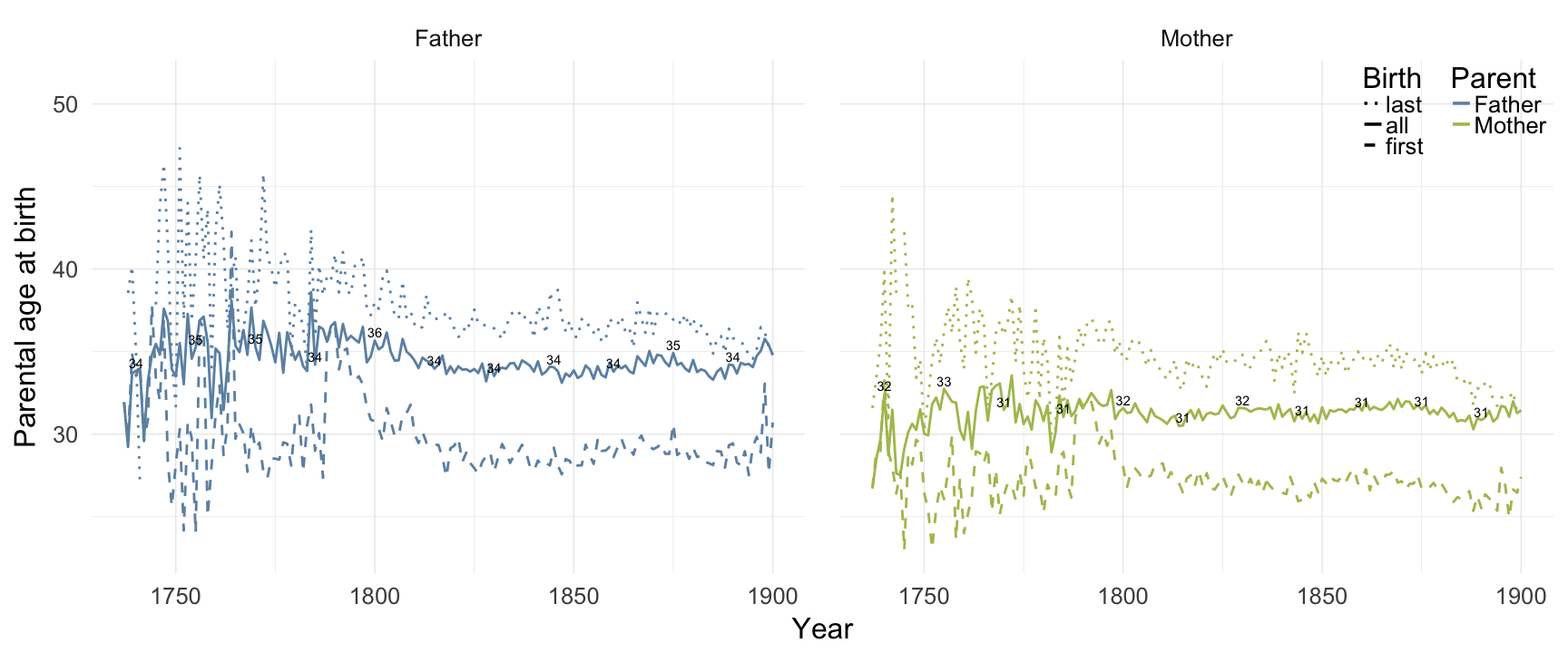

Sundsvall

ggplot(data = demo_trends_sundsvall) + 
    geom_line(aes(x= Year, y = first, linetype = "first", colour = Parent),  size = 1) + 
  geom_line(aes(x = Year, y = all, linetype = "all", colour = Parent), size = 1) +
    geom_line(aes(x= Year, y = last, linetype = "last", colour = Parent),size = 1) + 
    scale_colour_manual(values = c(Father = "#6c92b2", Mother = "#aec05d")) + 
    scale_linetype_manual("Birth", breaks = c("last", "all","first"), values = c( "solid","dashed", "dotted")) +
    scale_y_continuous("Parental age at birth") + 
        geom_text(aes(x = Year, y = all + 0.5, 
                                    label = ifelse(Year %% 15 == 0, round(all), NA))) + 
    facet_wrap(~ Parent) +
    desc_theme + theme(legend.position = c(1,1),
  legend.justification = c(1,1), 
  legend.box = "horizontal",
  panel.margin = unit(2, "lines"))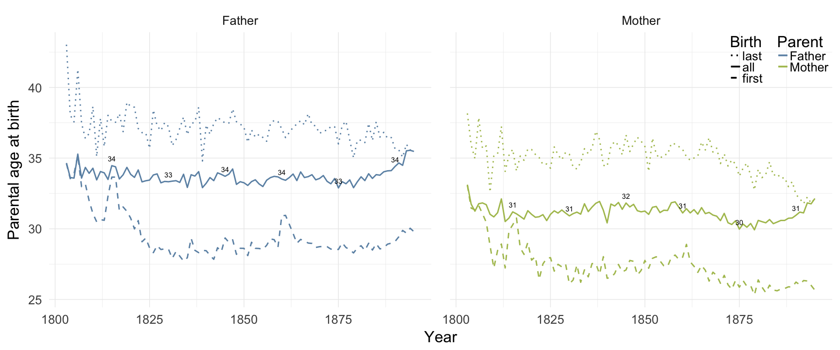

Norra inländs

ggplot(data = demo_trends_norra) + 
    geom_line(aes(x= Year, y = first, linetype = "first", colour = Parent),  size = 1) + 
  geom_line(aes(x = Year, y = all, linetype = "all", colour = Parent), size = 1) +
    geom_line(aes(x= Year, y = last, linetype = "last", colour = Parent),size = 1) + 
    scale_colour_manual(values = c(Father = "#6c92b2", Mother = "#aec05d")) + 
    scale_linetype_manual("Birth", breaks = c("last", "all","first"), values = c( "solid","dashed", "dotted")) +
    scale_y_continuous("Parental age at birth") + 
        geom_text(aes(x = Year, y = all + 0.5, 
                                    label = ifelse(Year %% 15 == 0, round(all), NA))) + 
    facet_wrap(~ Parent) +
    desc_theme + theme(legend.position = c(1,1),
  legend.justification = c(1,1), 
  legend.box = "horizontal",
  panel.margin = unit(2, "lines"))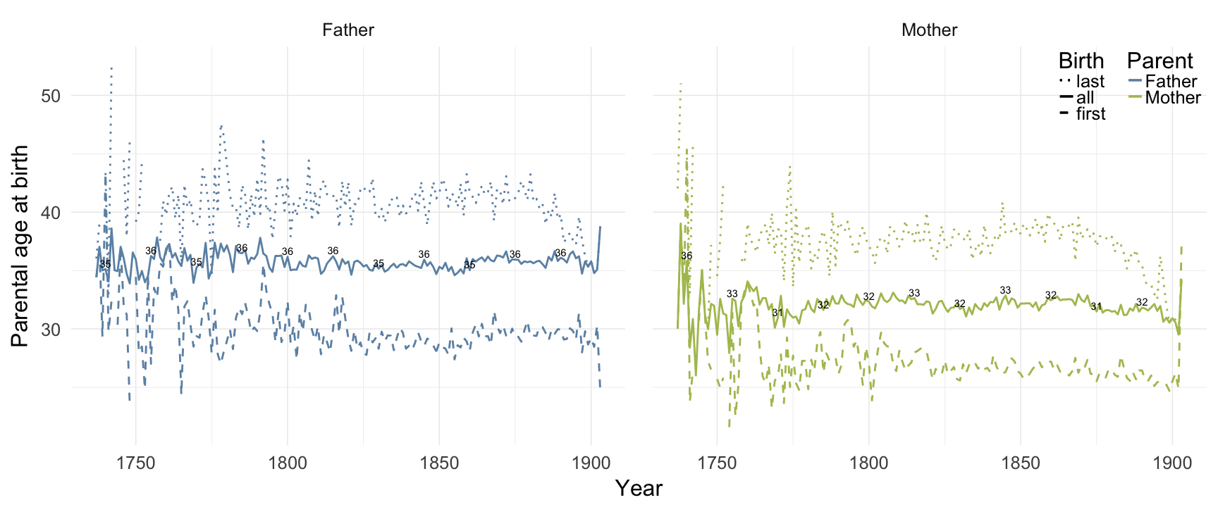

Skellefteå

ggplot(data = demo_trends_skelleftea) + 
    geom_line(aes(x= Year, y = first, linetype = "first", colour = Parent),  size = 1) + 
  geom_line(aes(x = Year, y = all, linetype = "all", colour = Parent), size = 1) +
    geom_line(aes(x= Year, y = last, linetype = "last", colour = Parent),size = 1) + 
    scale_colour_manual(values = c(Father = "#6c92b2", Mother = "#aec05d")) + 
    scale_linetype_manual("Birth", breaks = c("last", "all","first"), values = c( "solid","dashed", "dotted")) +
    scale_y_continuous("Parental age at birth") + 
        geom_text(aes(x = Year, y = all + 0.5, 
                                    label = ifelse(Year %% 15 == 0, round(all), NA))) + 
    facet_wrap(~ Parent) +
    desc_theme + theme(legend.position = c(1,1),
  legend.justification = c(1,1), 
  legend.box = "horizontal",
  panel.margin = unit(2, "lines"))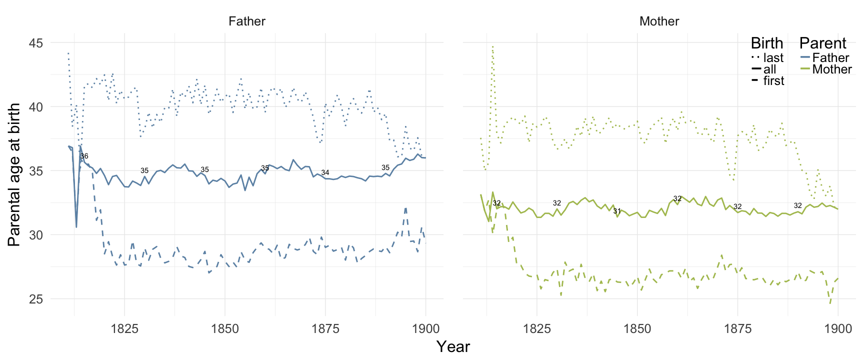

Missingness patterns

The first table shows the number of missings per variable, the second table, using the indexes from the first, shows missings in which variables tend to occur together. Most variables of interest in this study are derived from these dates and so these patterns can show many cases did not have the data to calculate e.g. paternal loss (those lacking either the father’s death date, the anchor’s birth date or both).

pander_escape(missingness_patterns(ddb[, list(
    bdate, ddate, bdate.Father, ddate.Father, bdate.Mother, ddate.Mother
    )]))

##  index          col missings
##      1        ddate   192778
##      2 ddate.Mother   182758
##      3 ddate.Father   176052
##      4 bdate.Father    11168
##      5 bdate.Mother    11136

Pattern	Freq	Culprit
1_2_3____	117430
1________	34786	ddate
_________	32303	_
__2_3____	26521
1_2______	18942
1___3____	13413
__2______	8595	ddate.Mother
____3____	7427	ddate.Father
1_2_3_4_5	7344
__2_3_4_5	3119
1_2_3___5	274
1_2_3_4__	270
______4__	76	bdate.Father
1_____4__	66
__2_3_4__	62
1_2_____5	60
________5	53	bdate.Mother
__2_3___5	50
1_______5	45
____3_4__	38
1_____4_5	35
1___3_4__	34
__2_____5	28
______4_5	26
1___3_4_5	24
____3___5	23
1_2___4__	22
1_2___4_5	21
1___3___5	12
__2___4_5	11
____3_4_5	11
__2___4__	9

Correlations between variables

round(cor(ddb[, list(
    paternalage, maternalage, birthorder, nr.siblings, children, grandchildren, byear, byear.Father, age_at_1st_child, age_at_last_child
    )], use = "pairwise.complete.obs"),2)

	paternalage	maternalage	birthorder	nr.siblings	children	grandchildren	byear	byear.Father	age_at_1st_child	age_at_last_child
paternalage	1	0.61	0.55	0.18	0	0	-0.01	-0.27	0.02	0.02
maternalage	0.61	1	0.6	0.13	0.01	0	-0.02	-0.18	0.01	0
birthorder	0.55	0.6	1	0.62	0	-0.02	0.11	-0.04	0.01	0.02
nr.siblings	0.18	0.13	0.62	1	0.1	0.04	-0.01	-0.06	0.04	0.08
children	0	0.01	0	0.1	1	0.51	-0.29	-0.28	-0.2	0.68
grandchildren	0	0	-0.02	0.04	0.51	1	-0.24	-0.24	-0.08	0.31
byear	-0.01	-0.02	0.11	-0.01	-0.29	-0.24	1	0.97	-0.17	-0.37
byear.Father	-0.27	-0.18	-0.04	-0.06	-0.28	-0.24	0.97	1	-0.17	-0.35
age_at_1st_child	0.02	0.01	0.01	0.04	-0.2	-0.08	-0.17	-0.17	1	0.46
age_at_last_child	0.02	0	0.02	0.08	0.68	0.31	-0.37	-0.35	0.46	1

ggplot(data=ddb, aes(x = byear, y = paternalage)) + 
    geom_linerange(stat = "summary", fun.data = "median_hilow", colour = "#aec05d") + 
    geom_pointrange(stat = "summary", fun.data = "mean_cl_boot", colour = "#6c92b2") + 
    facet_wrap(~ region, ncol = 1) + 
    desc_theme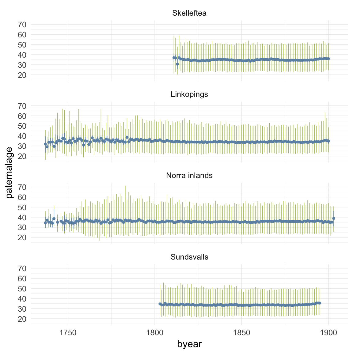

ggplot(data=ddb, aes(x = byear, y = maternalage)) + 
    geom_linerange(stat = "summary", fun.data = "median_hilow", colour = "#aec05d") + 
    geom_pointrange(stat = "summary", fun.data = "mean_cl_boot", colour = "#6c92b2") + 
    facet_wrap(~ region, ncol = 1) + 
    desc_theme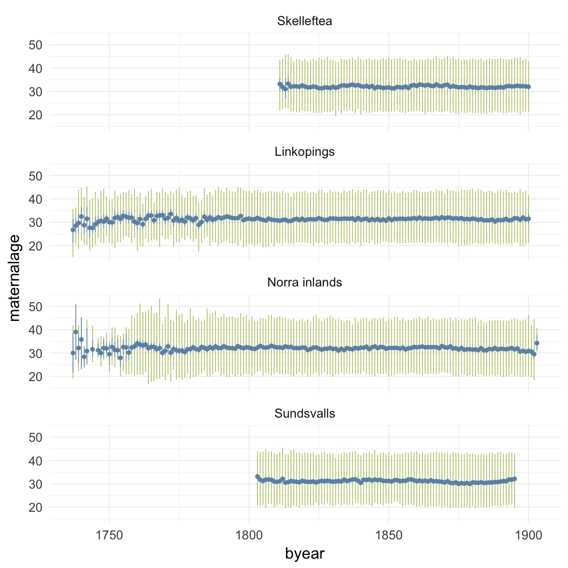

ggplot(data=ddb, aes(x = byear, y = age_at_1st_child)) + 
    geom_linerange(stat = "summary", fun.data = "median_hilow", colour = "#aec05d") + 
    geom_pointrange(stat = "summary", fun.data = "mean_cl_boot", colour = "#6c92b2") + 
    facet_wrap(~ region, ncol = 1) + 
    desc_theme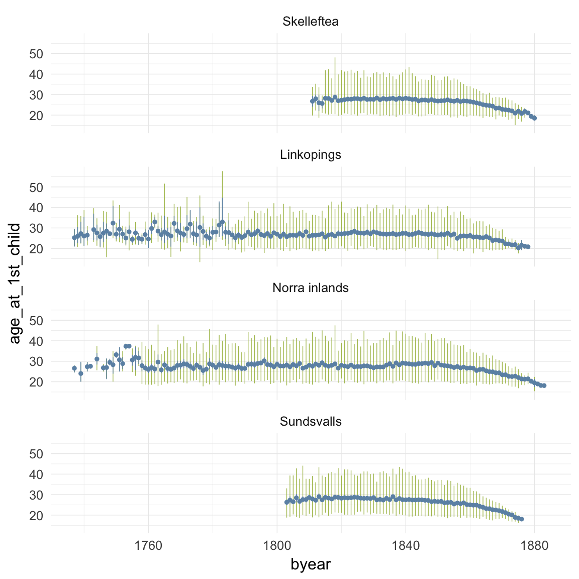

ggplot(data=ddb, aes(x = byear, y = age_at_last_child)) + 
    geom_linerange(stat = "summary", fun.data = "median_hilow", colour = "#aec05d") + 
    geom_pointrange(stat = "summary", fun.data = "mean_cl_boot", colour = "#6c92b2") + 
    facet_wrap(~ region, ncol = 1) + 
    desc_theme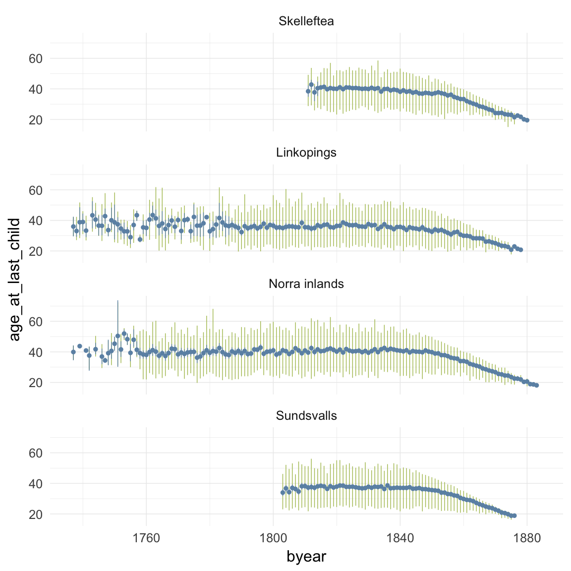

ggplot(data=ddb, aes(x = byear, y = children)) + 
    geom_linerange(stat = "summary", fun.data = "median_hilow", colour = "#aec05d") + 
    geom_pointrange(stat = "summary", fun.data = "mean_cl_boot", colour = "#6c92b2") + 
    facet_wrap(~ region, ncol = 1) + 
    desc_theme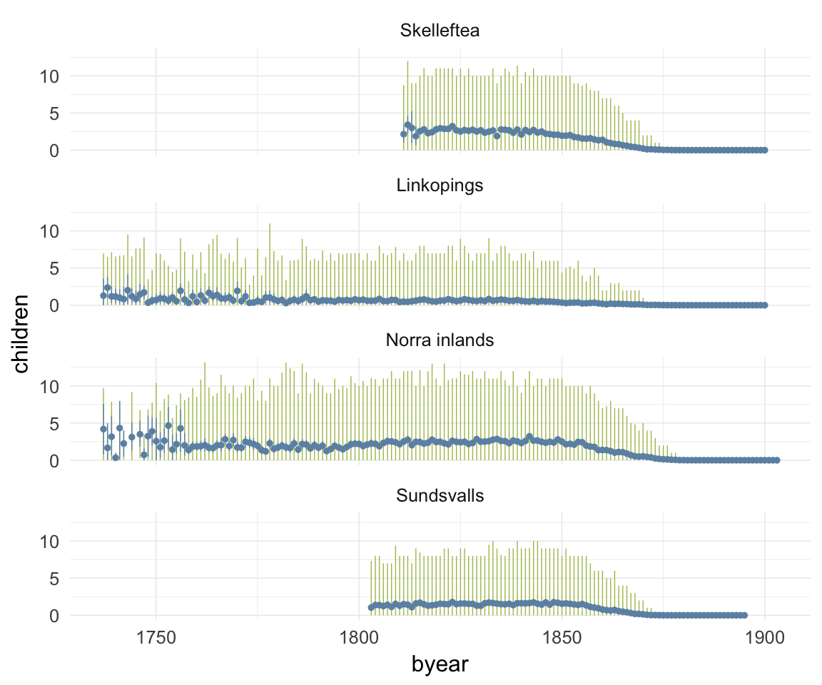

ggplot(data=ddb, aes(x = byear, y = survive1y)) + 
    geom_pointrange(stat = "summary", fun.data = "mean_cl_boot", colour = "#aec05d") + 
    facet_wrap(~ region, ncol = 1) + 
    desc_theme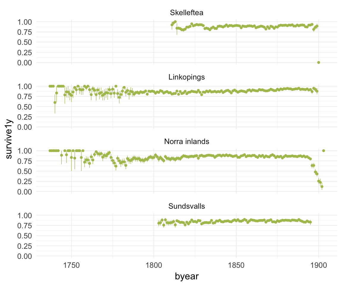

ggplot(data=ddb, aes(x = byear, y = surviveR)) + 
    geom_pointrange(stat = "summary", fun.data = "mean_cl_boot", colour = "#aec05d") + 
    facet_wrap(~ region, ncol = 1) + 
    desc_theme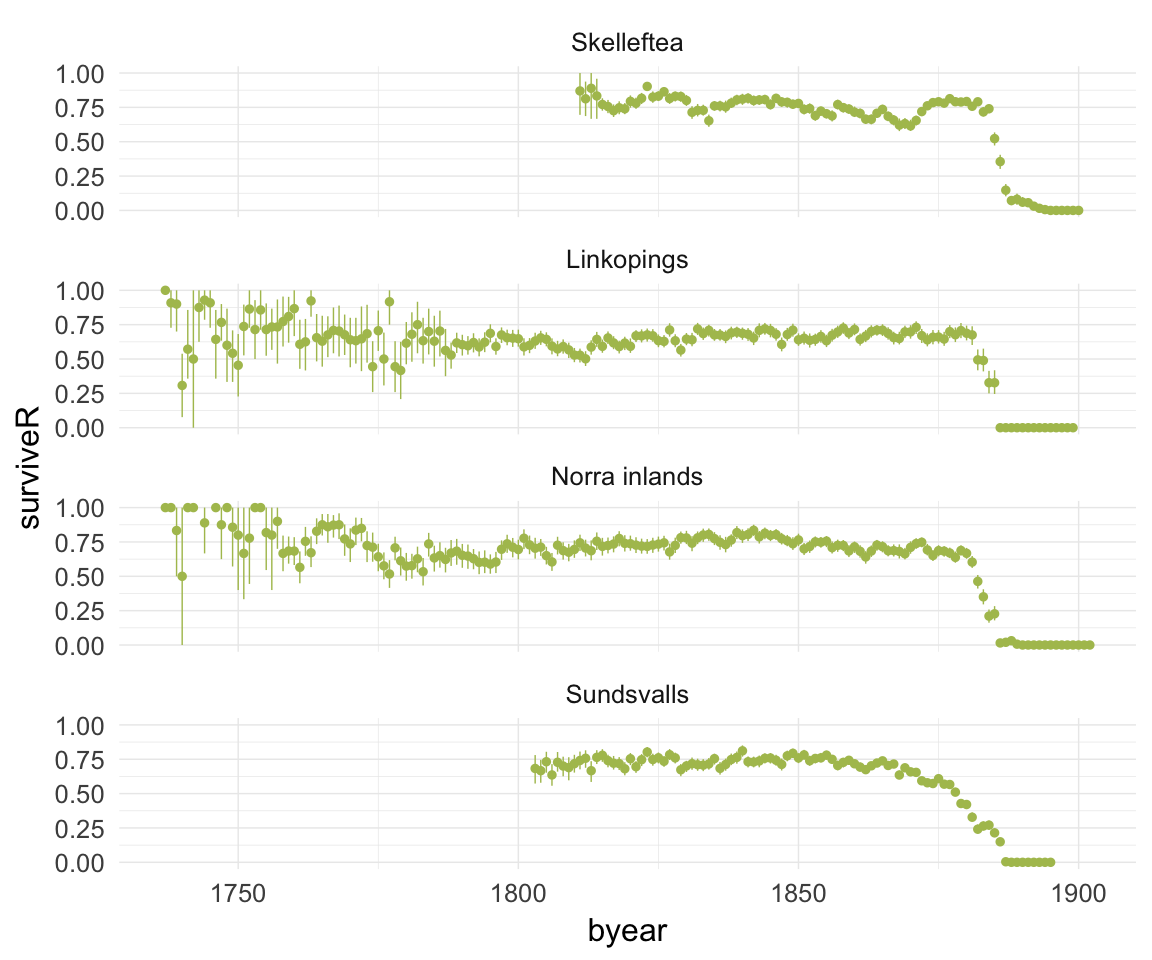

ggplot(data=ddb, aes(x = children, y = grandchildren)) + 
    geom_jitter(colour = "#aec05d", alpha = I(0.1)) + 
    geom_pointrange(stat = "summary", fun.data = "median_hilow", colour = "#6c92b2") +
    geom_smooth(method = "glm", formula = y ~ poly(x,3), colour = "#6e85b0") + 
    desc_theme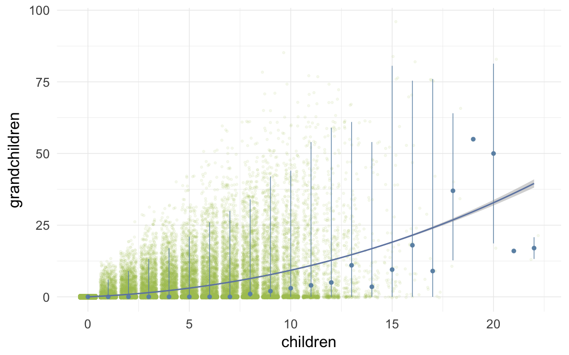

ggplot(data=ddb, aes(x = children, y = children.survivingR)) + 
    geom_jitter(colour = "#aec05d", alpha = I(0.1)) + 
    geom_pointrange(stat = "summary", fun.data = "median_hilow", colour = "#6c92b2") +
    geom_smooth(method = "glm", formula = y ~ poly(x,3), colour = "#6e85b0") + 
    desc_theme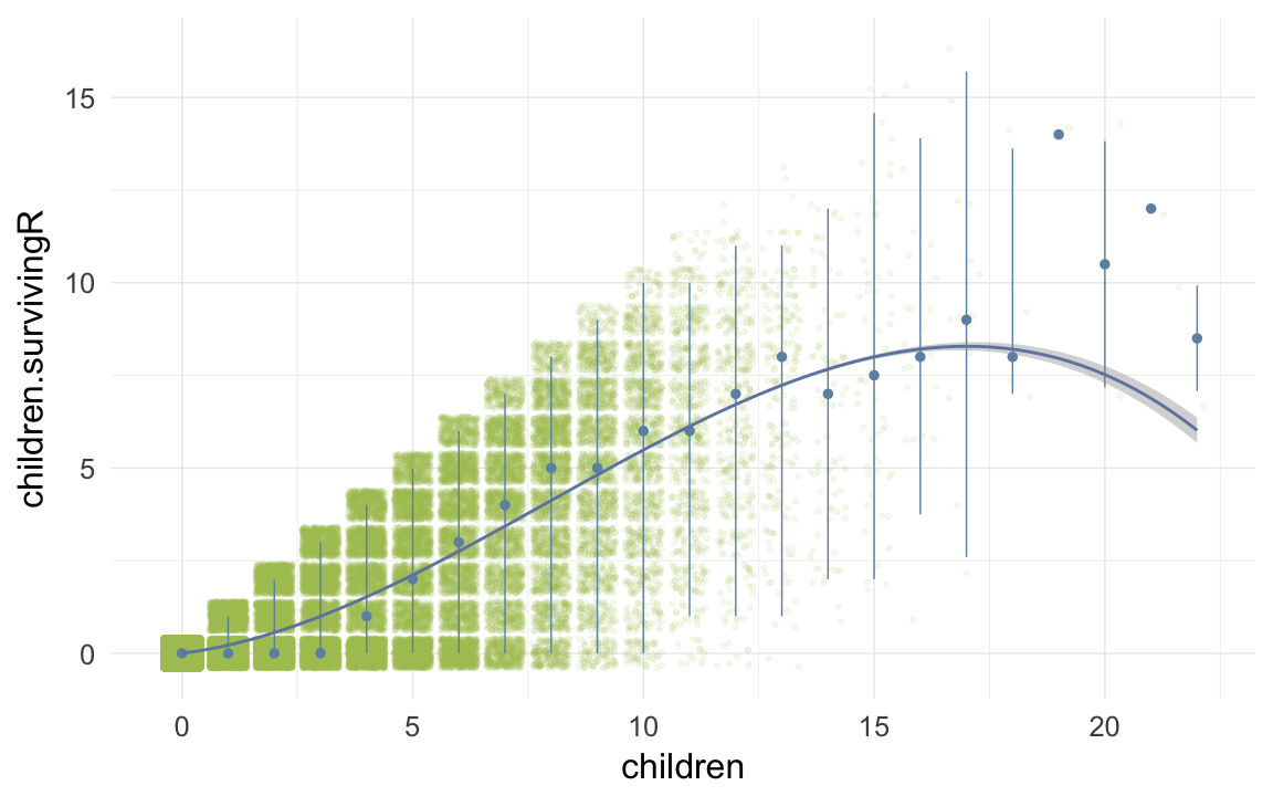

ggplot(data=ddb, aes(x = round(age), y = children)) + 
    geom_jitter(colour = "#aec05d", alpha = I(0.1)) + 
    geom_pointrange(stat = "summary", fun.data = "mean_cl_boot", colour = "#6c92b2") +
    geom_smooth(colour = "#6e85b0") + 
    xlab("Age") +
    ylab("Number of children") +
    desc_theme

ggplot(data=ddb[children>0,], aes(x = round(age), y = children)) + 
    geom_jitter(colour = "#aec05d", alpha = I(0.1)) + 
    geom_pointrange(stat = "summary", fun.data = "mean_cl_boot", colour = "#6c92b2") +
    geom_smooth(colour = "#6e85b0") + 
    xlab("Age") +
    ylab("Number of children") +
    desc_theme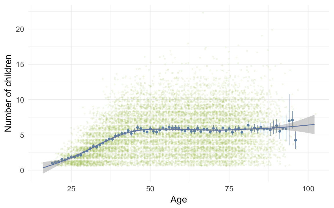

plot_zero_infl(ddb[ spouses > 0, ]$children)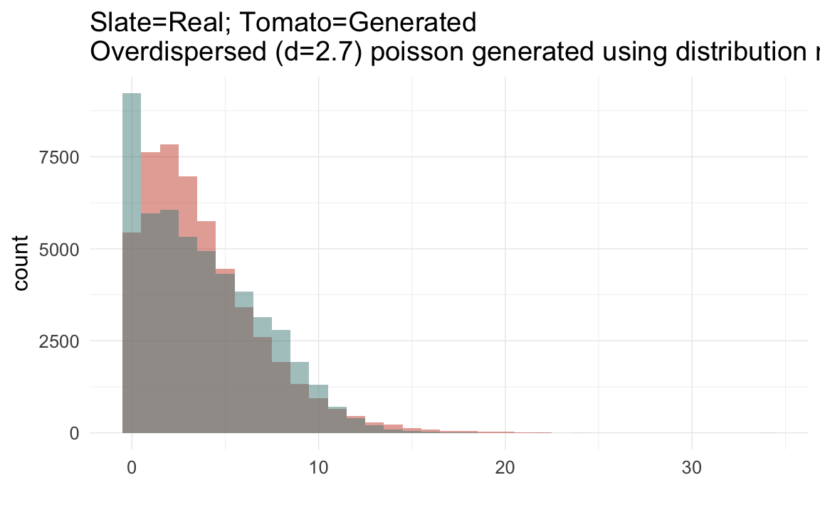

ggplot(data=ddb, aes(x = paternalage.factor, y = survive1y)) + 
    geom_pointrange(stat = "summary", fun.data = "mean_cl_boot", colour = "#aec05d") + 
    facet_wrap(~ region, ncol = 1) + 
    desc_theme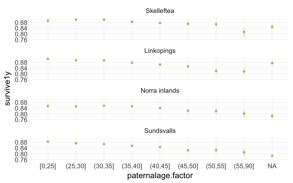

ggplot(data=ddb[spouses > 0, ], aes(x = paternalage.factor, y = children)) + 
    geom_pointrange(stat = "summary", fun.data = "mean_cl_boot", colour = "#aec05d") + 
    facet_wrap(~ region) + 
    desc_theme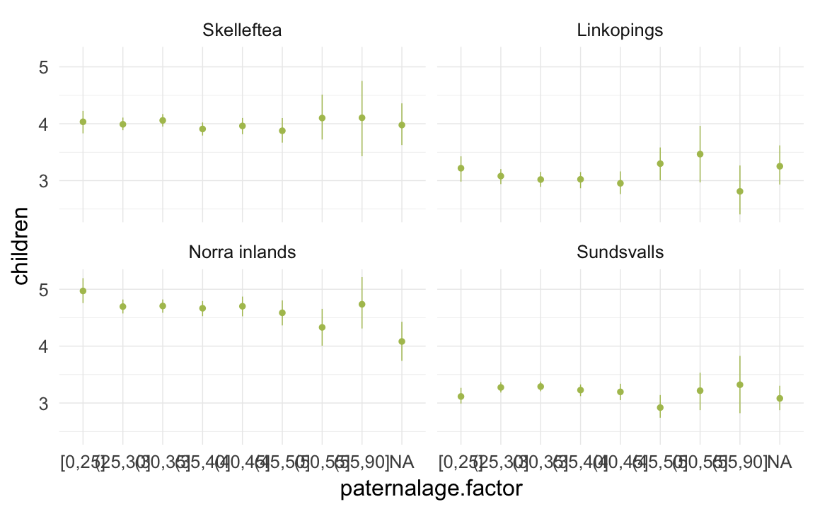

Opportunities for selection

ddb.1$birth.decade = round(ddb.1$byear/5)*5

episodes = ddb.1 %>%
    filter(!is.na(male) | !is.na(survive1y) | !is.na(ever_married)) %>% 
    group_by(region, birth.decade) %>%
    summarise(
        "Population size" = as.numeric(length(idIndividu)),
        "0. Number of children" = ifelse(between(birth.decade, 1735,1845), cva(children), NA_real_ ), 
        "1. Surviving first year" = cva_bin(survive1y),
        "2. Surviving to 15" = ifelse(between(birth.decade, 1735,1865), cva_bin(surviveR[survive1y==T]), NA_real_ ),
        "3. Ever married" = ifelse(between(birth.decade, 1735,1845), cva_bin(ever_married[surviveR==1]), NA_real_ ), 
        "4. Number of children" = ifelse(between(birth.decade, 1735,1845), cva(children[ever_married==1]), NA_real_ ), 
        "5. Grandchildren" = ifelse(between(birth.decade, 1735,1800), cva(grandchildren[children>0]), NA_real_ )
        ) %>%
    data.table()
data.frame(episodes[order(birth.decade), ])

region	birth.decade	Population.size	X0..Number.of.children	X1..Surviving.first.year	X2..Surviving.to.15	X3..Ever.married	X4..Number.of.children	X5..Grandchildren
Norra inlands	1735	5	1.043	0	0	0.5	0.8137	0.9742
Linkopings	1735	4	2	0	0	1	1.414	NA
Norra inlands	1740	14	1.358	0	0.4264	0.6124	0.7929	0.6621
Linkopings	1740	52	1.951	0.378	0.4663	0.6614	0.7308	1.928
Norra inlands	1745	25	1.139	0.2085	0	0.5423	0.7485	0.7598
Linkopings	1745	63	1.589	0.2626	0.2526	0.7878	0.7906	1.236
Norra inlands	1750	32	1.084	0.3333	0.3693	0.3974	0.5333	1.144
Linkopings	1750	73	2.459	0.4247	0.4822	1.124	0.9263	1.116
Norra inlands	1755	36	1.035	0.1741	0.1826	0.5517	0.564	0.6129
Linkopings	1755	82	1.825	0.2279	0.4344	0.7785	0.8655	1.375
Norra inlands	1760	215	1.483	0.543	0.3115	0.6292	0.6615	1.108
Linkopings	1760	80	1.953	0.1987	0.4758	0.9813	0.8485	2.041
Norra inlands	1765	262	1.367	0.3248	0.2861	0.5436	0.67	1.137
Linkopings	1765	100	1.559	0.4035	0.417	0.7303	0.7385	1.138
Norra inlands	1770	221	1.295	0.3196	0.2357	0.6297	0.6359	0.8947
Linkopings	1770	94	1.653	0.3922	0.3665	0.9005	0.7137	1.399
Norra inlands	1775	316	1.585	0.5634	0.4038	0.6025	0.7107	0.9836
Linkopings	1775	92	2.652	0.3441	0.5547	1	1.14	1.912
Norra inlands	1780	353	1.494	0.5245	0.3896	0.598	0.7174	1.005
Linkopings	1780	110	2.271	0.4909	0.6045	0.6367	1.057	1.912
Norra inlands	1785	357	1.578	0.5345	0.4035	0.6948	0.6515	1.015
Linkopings	1785	97	1.711	0.3802	0.4082	0.8321	0.7986	1.207
Linkopings	1790	618	2.222	0.4728	0.497	0.9535	0.8412	1.496
Norra inlands	1790	436	1.529	0.5	0.4233	0.6619	0.6989	0.9597
Linkopings	1795	851	2.133	0.4366	0.4524	0.9599	0.8708	1.629
Norra inlands	1795	539	1.444	0.4899	0.4654	0.6357	0.6144	1.126
Linkopings	1800	969	2.039	0.4461	0.4219	0.9277	0.855	1.645
Norra inlands	1800	565	1.358	0.4138	0.3747	0.602	0.7088	1.014
Sundsvalls	1805	565	1.509	0.4607	0.4012	0.6354	0.7615	NA
Linkopings	1805	1145	2.169	0.4365	0.5072	0.9884	0.8675	NA
Norra inlands	1805	659	1.319	0.4923	0.3516	0.5391	0.6799	NA
Sundsvalls	1810	703	1.551	0.4919	0.2869	0.7103	0.7935	NA
Linkopings	1810	1251	2.354	0.4597	0.5665	1.001	0.9188	NA
Norra inlands	1810	728	1.227	0.4826	0.3199	0.5402	0.6182	NA
Skelleftea	1810	46	1.136	0.2132	0.3244	0.5571	0.6647	NA
Sundsvalls	1815	1244	1.473	0.4663	0.2884	0.7095	0.7409	NA
Linkopings	1815	1414	2.183	0.4588	0.4194	1.084	0.8261	NA
Norra inlands	1815	789	1.289	0.478	0.2964	0.5956	0.6524	NA
Skelleftea	1815	857	1.246	0.4595	0.2853	0.6481	0.5842	NA
Sundsvalls	1820	1668	1.45	0.5017	0.2599	0.7141	0.7115	NA
Linkopings	1820	1560	2.383	0.4522	0.4398	1.183	0.8688	NA
Norra inlands	1820	956	1.254	0.3879	0.3793	0.5706	0.6316	NA
Skelleftea	1820	1579	1.187	0.4203	0.2753	0.6091	0.5828	NA
Sundsvalls	1825	1911	1.373	0.4313	0.2764	0.6419	0.7502	NA
Linkopings	1825	1662	2.369	0.4057	0.4593	1.196	0.8712	NA
Norra inlands	1825	1058	1.288	0.414	0.4071	0.5383	0.6539	NA
Skelleftea	1825	1750	1.179	0.2906	0.2689	0.6323	0.6065	NA
Sundsvalls	1830	1826	1.459	0.4929	0.3112	0.6796	0.7363	NA
Linkopings	1830	1644	2.359	0.4318	0.4711	1.155	0.8886	NA
Norra inlands	1830	1164	1.204	0.373	0.3382	0.5638	0.6426	NA
Skelleftea	1830	1696	1.202	0.3729	0.3322	0.6256	0.5815	NA
Sundsvalls	1835	1713	1.442	0.463	0.3295	0.6306	0.7567	NA
Linkopings	1835	1670	2.325	0.4022	0.4047	1.239	0.8824	NA
Norra inlands	1835	1248	1.2	0.3925	0.3403	0.6155	0.5986	NA
Skelleftea	1835	1774	1.273	0.4554	0.3509	0.6374	0.5983	NA
Sundsvalls	1840	1711	1.448	0.4336	0.2814	0.6772	0.7818	NA
Linkopings	1840	1581	2.389	0.4201	0.4079	1.243	0.9058	NA
Norra inlands	1840	1322	1.214	0.3732	0.2801	0.635	0.6429	NA
Skelleftea	1840	1667	1.268	0.3885	0.2834	0.7023	0.6236	NA
Sundsvalls	1845	2024	1.503	0.4281	0.3107	0.7389	0.7722	NA
Linkopings	1845	1463	2.589	0.3775	0.4259	1.352	0.9412	NA
Norra inlands	1845	1578	1.285	0.3673	0.3193	0.6863	0.6562	NA
Skelleftea	1845	1909	1.261	0.3374	0.3398	0.6869	0.6347	NA
Sundsvalls	1850	752	NA	0.3771	0.2852	NA	NA	NA
Linkopings	1850	551	NA	0.3736	0.4029	NA	NA	NA
Norra inlands	1850	670	NA	0.4129	0.3856	NA	NA	NA
Skelleftea	1850	778	NA	0.3494	0.3658	NA	NA	NA

save(episodes, file = "coefs/ddb_episodes.rdata")

(episodes.plot = ggplot(melt(episodes,id.vars=c('birth.decade','region'), na.rm = T)) + geom_line(aes(x=birth.decade, y=value)) + facet_grid(variable ~ region,scales='free_y')) + mymin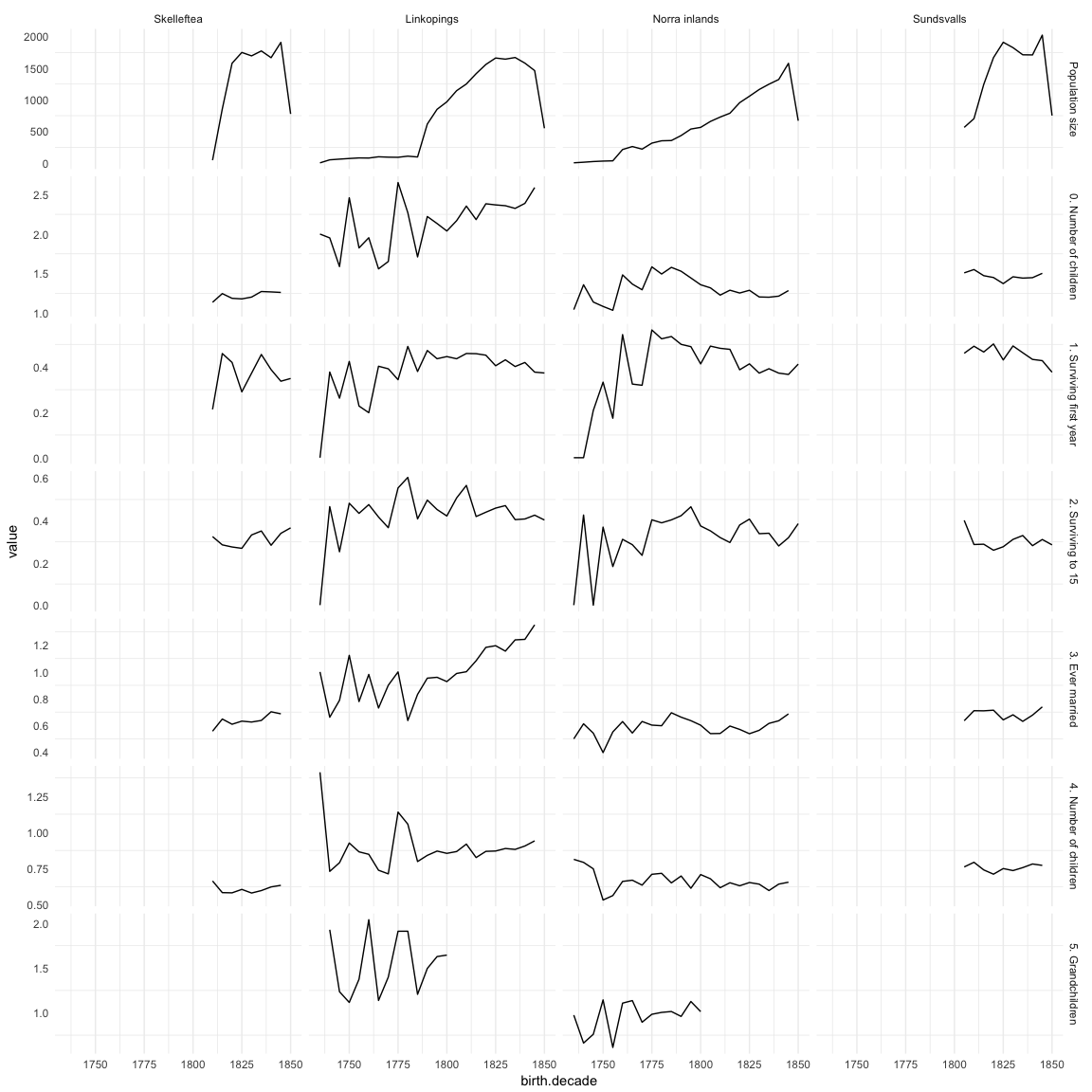

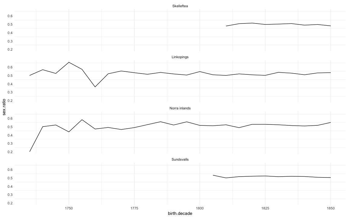
Sex ratio

(sex.ratio = ddb.1 %>% 
    filter(!is.na(male)) %>% 
    mutate(male = as.numeric(as.character(male))) %>%
    group_by(birth.decade, region) %>% 
    summarise(sex.ratio = sum(male)/length(male)) %>%
    data.frame()
)

birth.decade	region	sex.ratio
1845	Sundsvalls	0.5067
1850	Sundsvalls	0.5033
1805	Sundsvalls	0.5319
1810	Sundsvalls	0.4993
1820	Sundsvalls	0.5198
1835	Sundsvalls	0.5188
1825	Sundsvalls	0.5225
1830	Sundsvalls	0.5146
1815	Sundsvalls	0.5149
1840	Sundsvalls	0.5167
1805	Linkopings	0.5079
1810	Linkopings	0.5004
1800	Linkopings	0.5459
1815	Linkopings	0.5184
1795	Linkopings	0.5047
1830	Linkopings	0.5369
1835	Linkopings	0.5275
1825	Linkopings	0.5012
1840	Linkopings	0.5079
1845	Linkopings	0.5304
1790	Linkopings	0.5178
1820	Linkopings	0.5074
1850	Linkopings	0.5336
1835	Norra inlands	0.5132
1840	Norra inlands	0.5083
1805	Norra inlands	0.5106
1815	Norra inlands	0.4879
1745	Norra inlands	0.52
1750	Norra inlands	0.4375
1755	Norra inlands	0.5833
1760	Norra inlands	0.472
1765	Norra inlands	0.4904
1780	Norra inlands	0.5241
1800	Norra inlands	0.515
1810	Norra inlands	0.522
1830	Norra inlands	0.5224
1845	Norra inlands	0.5155
1825	Norra inlands	0.5279
1785	Norra inlands	0.559
1795	Norra inlands	0.5578
1790	Norra inlands	0.5196
1820	Norra inlands	0.5278
1775	Norra inlands	0.4889
1770	Norra inlands	0.4658
1850	Norra inlands	0.5502
1740	Norra inlands	0.5
1735	Norra inlands	0.2
1845	Skelleftea	0.4968
1850	Skelleftea	0.4803
1830	Skelleftea	0.5018
1835	Skelleftea	0.5076
1840	Skelleftea	0.489
1820	Skelleftea	0.5139
1825	Skelleftea	0.4971
1815	Skelleftea	0.5064
1810	Skelleftea	0.4783
1735	Linkopings	0.5
1740	Linkopings	0.5686
1745	Linkopings	0.5238
1775	Linkopings	0.5326
1780	Linkopings	0.5138
1785	Linkopings	0.5361
1750	Linkopings	0.6575
1755	Linkopings	0.5732
1770	Linkopings	0.5532
1760	Linkopings	0.3625
1765	Linkopings	0.52

ggplot(na.omit(sex.ratio)) + geom_line(aes(x=birth.decade, y=sex.ratio)) + facet_wrap(~ region, ncol=1) + mymin

Demographic data base Sweden

Loading details

Variable descriptives

Whole population (N = 271130)

Linköping

Sundsvall

Norra inländs

Skellefteå

included sample (N = 56947)

Linköping

Sundsvall

Norra inländs

Skellefteå

Number of families with varying numbers of siblings available for comparison

Reproductive timing

Linköping

Sundsvall

Norra inländs

Skellefteå

Missingness patterns

Correlations between variables

Opportunities for selection

Sex ratio