Krummhörn descriptives
Loading details
source("0__helpers.R")
opts_chunk$set(render = pander_handler, tidy=FALSE, autodep=TRUE, dev='png', fig.width=12, fig.height=7.5, cache = FALSE, warning = FALSE, message = FALSE)load("krmh.rdata")
desc_theme = theme_minimal(base_size = 24)
update_geom_defaults("bar", list(fill = "#6c92b2", alpha = 1/2))
krmh = data.table(krmh)
krmh.1 = data.table(krmh.1)
demo_trends = aggDemoTrends(krmh)
mymin = theme_minimal() +theme(panel.grid.major.y =element_blank(),panel.grid.major.x = element_line(colour="#eeeeee"))
krmh[, paternalage := 10 * paternalage]; krmh.1[, paternalage := 10 * paternalage]krmh[, maternalage := 10 * maternalage]; krmh.1[, maternalage := 10 * maternalage]krmh[, age := 10 * age]; krmh.1[, age := 10 * age]krmh[, age_at_1st_child := 10 * age_at_1st_child]; krmh.1[, age_at_1st_child := 10 * age_at_1st_child]krmh[, age_at_last_child := 10 * age_at_last_child]; krmh.1[, age_at_last_child := 10 * age_at_last_child]krmh[, byear := year(bdate)]; krmh.1[, byear := year(bdate)]krmh[, byear.Father := year(bdate.Father)];krmh.1[, byear.Father := year(bdate.Father)]Variable descriptives
The following statistics refer to all births. This means that e.g. the percentage of ever married people includes some who died before they had a chance at marriage.
Whole population (N = 80808)
descriptives = psych::describe(krmh[, list(
    paternalage, maternalage, nr.siblings, dependent_sibs_f5y, age, spouses, children, grandchildren, byear, byear.Father, age_at_1st_child, age_at_last_child  )])
round(data.frame(descriptives)[,2:12],2)| n | mean | sd | median | trimmed | mad | min | max | range | skew | kurtosis | |
|---|---|---|---|---|---|---|---|---|---|---|---|
| paternalage | 35907 | 34.97 | 7.35 | 34.09 | 34.5 | 7.39 | 16.07 | 74.48 | 58.4 | 0.65 | 0.45 |
| maternalage | 36371 | 31.49 | 5.97 | 31.15 | 31.36 | 6.63 | 14.62 | 54.62 | 40.01 | 0.18 | -0.65 |
| nr.siblings | 80808 | 3.94 | 2.91 | 4 | 3.76 | 2.97 | 0 | 17 | 17 | 0.46 | -0.17 |
| dependent_sibs_f5y | 80808 | 1.74 | 1.39 | 2 | 1.62 | 1.48 | 0 | 14 | 14 | 0.82 | 1.76 |
| age | 24973 | 20.03 | 26.2 | 5.29 | 15.38 | 7.79 | 0 | 100.8 | 100.8 | 1.21 | 0.07 |
| spouses | 80808 | 0.36 | 0.57 | 0 | 0.27 | 0 | 0 | 5 | 5 | 1.48 | 2.08 |
| children | 80808 | 1.12 | 2.36 | 0 | 0.5 | 0 | 0 | 20 | 20 | 2.27 | 4.74 |
| grandchildren | 80808 | 1.26 | 4.21 | 0 | 0.09 | 0 | 0 | 62 | 62 | 4.38 | 23.1 |
| byear | 75018 | 1796 | 55.27 | 1800 | 1798 | 63.75 | 1572 | 1932 | 360 | -0.29 | -0.6 |
| byear.Father | 52616 | 1776 | 46.25 | 1779 | 1778 | 53.37 | 1544 | 1889 | 345 | -0.27 | -0.46 |
| age_at_1st_child | 15943 | 27.8 | 5.2 | 27.04 | 27.32 | 4.51 | 14.62 | 67.64 | 53.03 | 1.2 | 3.01 |
| age_at_last_child | 15943 | 37.28 | 7.48 | 37.85 | 37.28 | 7.32 | 14.62 | 74.48 | 59.86 | 0.1 | 0.23 |
describeBin(krmh[, list(survive1y, surviveR, ever_married)])| n | mean | sd | |
|---|---|---|---|
| survive1y | 57490 | 0.87 | 0.11 |
| surviveR | 57490 | 0.73 | 0.2 |
| ever_married | 80808 | 0.32 | 0.22 |
pander(xtabs(~ paternal_loss, krmh), caption = "Paternal loss at age")| later | [0,1] | (1,5] | (5,10] | (10,15] | (15,20] | (20,25] | (25,30] | (30,35] | (35,40] | (40,45] | unclear |
|---|---|---|---|---|---|---|---|---|---|---|---|
| 5230 | 1448 | 3332 | 4638 | 4937 | 5164 | 5238 | 5302 | 5006 | 4353 | 2854 | 33306 |
pander(xtabs(~ maternal_loss, krmh), caption = "Maternal loss at age")| later | [0,1] | (1,5] | (5,10] | (10,15] | (15,20] | (20,25] | (25,30] | (30,35] | (35,40] | (40,45] | unclear |
|---|---|---|---|---|---|---|---|---|---|---|---|
| 8567 | 1822 | 3297 | 4023 | 3853 | 3675 | 3919 | 4374 | 4768 | 5079 | 3739 | 33692 |
included sample (N = 14034)
descriptives = psych::describe(krmh.1[, list(
    paternalage, maternalage, nr.siblings, dependent_sibs_f5y, age, spouses, children, grandchildren, byear, byear.Father, age_at_1st_child, age_at_last_child  )])
round(data.frame(descriptives)[,2:12],2)| n | mean | sd | median | trimmed | mad | min | max | range | skew | kurtosis | |
|---|---|---|---|---|---|---|---|---|---|---|---|
| paternalage | 14034 | 34.97 | 7.58 | 33.96 | 34.44 | 7.61 | 16.93 | 70.57 | 53.65 | 0.67 | 0.33 |
| maternalage | 9472 | 31.17 | 5.83 | 30.77 | 31.02 | 6.41 | 15.22 | 49.08 | 33.86 | 0.21 | -0.62 |
| nr.siblings | 14034 | 5.03 | 2.56 | 5 | 4.94 | 2.97 | 0 | 15 | 15 | 0.42 | 0.32 |
| dependent_sibs_f5y | 14034 | 2.01 | 1.14 | 2 | 1.97 | 1.48 | 0 | 7 | 7 | 0.4 | 0.24 |
| age | 6984 | 23.46 | 27.53 | 8.32 | 19.48 | 12.3 | 0 | 100.8 | 100.8 | 0.94 | -0.56 |
| spouses | 14034 | 0.5 | 0.61 | 0 | 0.43 | 0 | 0 | 4 | 4 | 0.96 | 0.63 |
| children | 14034 | 1.79 | 2.81 | 0 | 1.22 | 0 | 0 | 18 | 18 | 1.49 | 1.35 |
| grandchildren | 14034 | 2.09 | 5.26 | 0 | 0.64 | 0 | 0 | 51 | 51 | 3.26 | 12.44 |
| byear | 14034 | 1794 | 27.04 | 1799 | 1796 | 31.13 | 1720 | 1834 | 114 | -0.52 | -0.61 |
| byear.Father | 14034 | 1759 | 27.66 | 1763 | 1761 | 32.62 | 1669 | 1812 | 143 | -0.43 | -0.59 |
| age_at_1st_child | 5215 | 28.04 | 5.18 | 27.28 | 27.58 | 4.53 | 15.22 | 66.39 | 51.17 | 1.1 | 2.45 |
| age_at_last_child | 5215 | 38.38 | 7.01 | 39.13 | 38.48 | 6.14 | 17.71 | 70.57 | 52.87 | -0.01 | 0.52 |
describeBin(krmh.1[, list(survive1y, surviveR, ever_married)])| n | mean | sd | |
|---|---|---|---|
| survive1y | 14034 | 0.87 | 0.11 |
| surviveR | 14034 | 0.72 | 0.2 |
| ever_married | 14034 | 0.44 | 0.25 |
pander(xtabs(~ paternal_loss, krmh.1), caption = "Paternal loss at age")| later | [0,1] | (1,5] | (5,10] | (10,15] | (15,20] | (20,25] | (25,30] | (30,35] | (35,40] | (40,45] | unclear |
|---|---|---|---|---|---|---|---|---|---|---|---|
| 1967 | 306 | 725 | 1074 | 1195 | 1350 | 1495 | 1623 | 1658 | 1578 | 1063 | 0 |
pander(xtabs(~ maternal_loss, krmh.1), caption = "Maternal loss at age")| later | [0,1] | (1,5] | (5,10] | (10,15] | (15,20] | (20,25] | (25,30] | (30,35] | (35,40] | (40,45] | unclear |
|---|---|---|---|---|---|---|---|---|---|---|---|
| 3037 | 429 | 846 | 1044 | 966 | 900 | 1012 | 1308 | 1482 | 1689 | 1321 | 0 |
Number of families with varying numbers of siblings available for comparison
crosstabs(krmh[!duplicated(idParents), ]$nr.siblings)| 0 | 1 | 2 | 3 | 4 | 5 | 6 | 7 | 8 | 9 | 10 | 11 | 12 | 13 | 14 | 15 | 16 | 17 |
|---|---|---|---|---|---|---|---|---|---|---|---|---|---|---|---|---|---|
| 13433 | 3467 | 2551 | 2292 | 1948 | 1623 | 1170 | 824 | 480 | 257 | 98 | 50 | 27 | 19 | 5 | 3 | 2 | 1 |
qplot(krmh[!duplicated(idParents), ]$nr.siblings, binwidth = 1) + xlab("Number of siblings per family") + desc_theme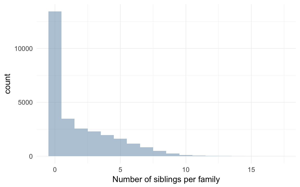
Missingness patterns
The first table shows the number of missings per variable, the second table, using the indexes from the first, shows missings in which variables tend to occur together. Most variables of interest in this study are derived from these dates and so these patterns can show many cases did not have the data to calculate e.g. paternal loss (those lacking either the father’s death date, the anchor’s birth date or both).
pander_escape(missingness_patterns(krmh[, list(
    bdate, ddate, bdate.Father, ddate.Father, bdate.Mother, ddate.Mother
    )]))
## index col missings
## 1 ddate 52229
## 2 ddate.Mother 32025
## 3 ddate.Father 31617
## 4 bdate.Father 28192
## 5 bdate.Mother 27849
## 6 bdate 5790| Pattern | Freq | Culprit |
|---|---|---|
| 1__________ | 19733 | ddate |
| ___________ | 12819 | _ |
| 1_2_3_4_5__ | 8735 | |
| 1_2_3______ | 5237 | |
| __2_3_4_5__ | 2732 | |
| 1_____4_5__ | 2350 | |
| 1_2________ | 2335 | |
| 1___3______ | 2087 | |
| __2_3______ | 2060 | |
| __2_3_4_5_6 | 2013 | |
| 1_2_3_4_5_6 | 1549 | |
| 1_____4____ | 1526 | |
| __2________ | 1394 | ddate.Mother |
| ____3______ | 1310 | ddate.Father |
| 1_______5__ | 1292 | |
| 1_2___4_5__ | 1211 | |
| 1___3_4____ | 1134 | |
| 1_2_____5__ | 1079 | |
| ______4_5__ | 1070 | |
| 1___3_4_5__ | 1008 | |
| ________5__ | 864 | bdate.Mother |
| ______4____ | 817 | bdate.Father |
| 1_2_3___5__ | 797 | |
| 1_2_3_4____ | 757 | |
| ____3_4____ | 580 | |
| __2_____5__ | 452 | |
| __2___4_5__ | 372 | |
| ______4_5_6 | 358 | |
| ____3_4_5__ | 327 | |
| __2_3_4____ | 277 | |
| 1_____4_5_6 | 274 | |
| __2_3___5__ | 254 | |
| 1_2___4_5_6 | 222 | |
| __________6 | 158 | bdate |
| 1___3_4_5_6 | 156 | |
| ____3_4_5_6 | 154 | |
| 1_________6 | 148 | |
| 1___3___5__ | 145 | |
| 1_2___4____ | 139 | |
| __2___4_5_6 | 118 | |
| ______4___6 | 96 | |
| ________5_6 | 83 | |
| ____3___5__ | 63 | |
| __2___4____ | 62 | |
| 1_2_____5_6 | 54 | |
| 1___3_4___6 | 53 | |
| 1_______5_6 | 53 | |
| 1_____4___6 | 35 | |
| __2_____5_6 | 35 | |
| 1_2_3_____6 | 34 | |
| ____3_4___6 | 33 | |
| 1___3_____6 | 31 | |
| ____3_____6 | 19 | |
| __2_______6 | 18 | |
| 1_2_______6 | 17 | |
| 1_2_3_4___6 | 16 | |
| __2_3_____6 | 16 | |
| 1_2_3___5_6 | 14 | |
| __2_3_4___6 | 11 | |
| __2_3___5_6 | 8 | |
| 1___3___5_6 | 5 | |
| __2___4___6 | 4 | |
| 1_2___4___6 | 3 | |
| ____3___5_6 | 2 |
Reproductive timing
ggplot(data = demo_trends[Year > 1680 & Year< 1900,]) +
    geom_line(aes(x= Year, y = first, linetype = "first", colour = Parent),  size = 1) +
  geom_line(aes(x = Year, y = all, linetype = "all", colour = Parent), size = 1) +
    geom_line(aes(x= Year, y = last, linetype = "last", colour = Parent),size = 1) +
    scale_colour_manual(values = c(Father = "#6c92b2", Mother = "#aec05d")) +
    scale_linetype_manual("Birth", breaks = c("last", "all","first"), values = c( "solid","dashed", "dotted")) +
    scale_y_continuous("Parental age at birth") +
        geom_text(aes(x = Year, y = all + 0.5,
                                    label = ifelse(Year %% 15 == 0, round(all), NA))) +
    facet_wrap(~ Parent) +
    desc_theme + theme(legend.position = c(1,1),
  legend.justification = c(1,1),
  legend.box = "horizontal",
  panel.margin = unit(2, "lines"))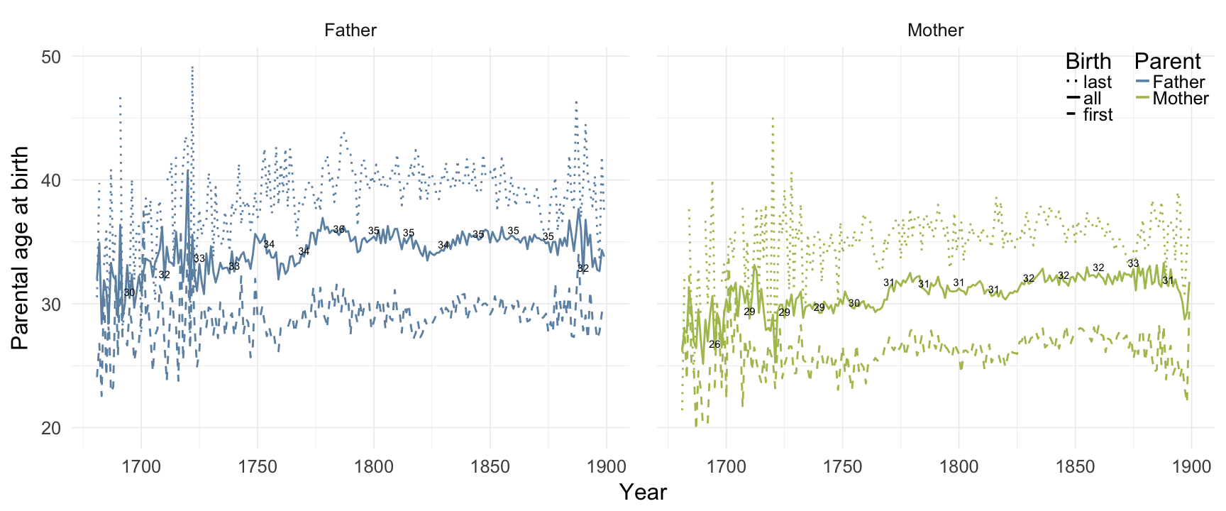
Correlations between variables
round(cor(krmh[, list(
    paternalage, maternalage, birthorder, nr.siblings, children, grandchildren, byear, byear.Father, age_at_1st_child, age_at_last_child
)], use = "pairwise.complete.obs"),2)| paternalage | maternalage | birthorder | nr.siblings | children | grandchildren | byear | byear.Father | age_at_1st_child | age_at_last_child | |
|---|---|---|---|---|---|---|---|---|---|---|
| paternalage | 1 | 0.63 | 0.56 | 0.14 | -0.04 | -0.02 | 0.05 | -0.12 | 0.04 | 0 |
| maternalage | 0.63 | 1 | 0.64 | 0.1 | -0.04 | -0.03 | 0.11 | 0 | 0.03 | 0 |
| birthorder | 0.56 | 0.64 | 1 | 0.67 | -0.03 | -0.02 | 0.1 | -0.04 | 0.02 | 0.02 |
| nr.siblings | 0.14 | 0.1 | 0.67 | 1 | 0.01 | 0 | 0.04 | -0.07 | 0.02 | 0.05 |
| children | -0.04 | -0.04 | -0.03 | 0.01 | 1 | 0.64 | -0.09 | -0.15 | -0.25 | 0.64 |
| grandchildren | -0.02 | -0.03 | -0.02 | 0 | 0.64 | 1 | -0.14 | -0.21 | -0.14 | 0.32 |
| byear | 0.05 | 0.11 | 0.1 | 0.04 | -0.09 | -0.14 | 1 | 0.99 | -0.04 | -0.19 |
| byear.Father | -0.12 | 0 | -0.04 | -0.07 | -0.15 | -0.21 | 0.99 | 1 | -0.08 | -0.21 |
| age_at_1st_child | 0.04 | 0.03 | 0.02 | 0.02 | -0.25 | -0.14 | -0.04 | -0.08 | 1 | 0.44 |
| age_at_last_child | 0 | 0 | 0.02 | 0.05 | 0.64 | 0.32 | -0.19 | -0.21 | 0.44 | 1 |
ggplot(data=krmh, aes(x = byear, y = paternalage)) +
    geom_linerange(stat = "summary", fun.data = "median_hilow", colour = "#aec05d") +
    geom_pointrange(stat = "summary", fun.data = "mean_cl_boot", colour = "#6c92b2") +
    desc_theme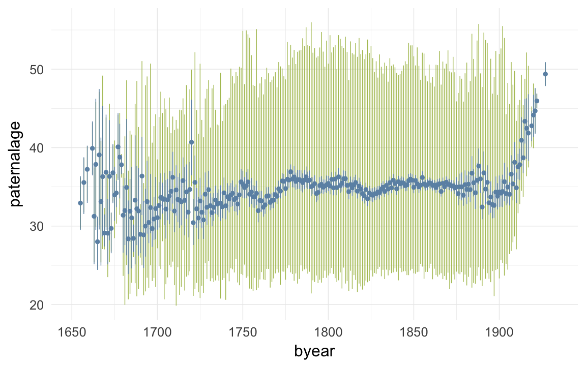
ggplot(data=krmh, aes(x = byear, y = age_at_1st_child)) +
    geom_linerange(stat = "summary", fun.data = "median_hilow", colour = "#aec05d") +
    geom_pointrange(stat = "summary", fun.data = "mean_cl_boot", colour = "#6c92b2") +
    desc_theme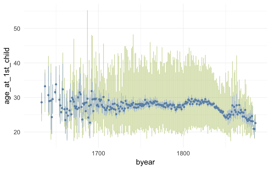
ggplot(data=krmh, aes(x = byear, y = age_at_last_child)) +
    geom_linerange(stat = "summary", fun.data = "median_hilow", colour = "#aec05d") +
    geom_pointrange(stat = "summary", fun.data = "mean_cl_boot", colour = "#6c92b2") +
    desc_theme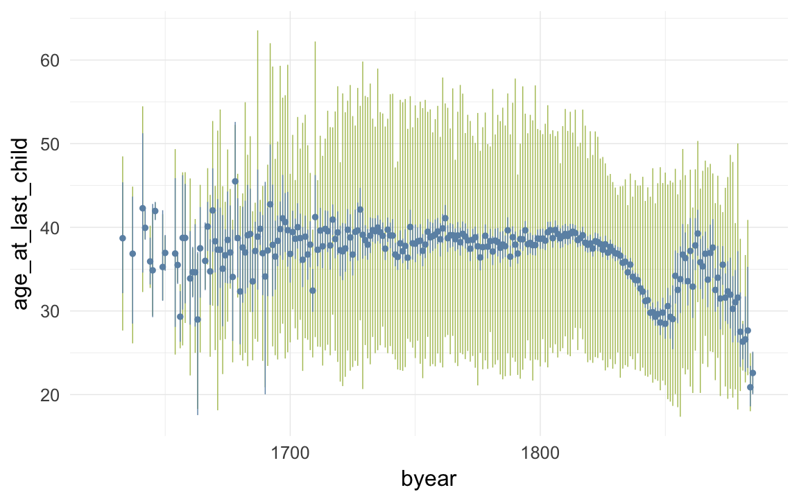
ggplot(data=krmh, aes(x = byear, y = children)) +
    geom_linerange(stat = "summary", fun.data = "median_hilow", colour = "#aec05d", na.rm=T) +
    geom_pointrange(stat = "summary", fun.data = "mean_cl_boot", colour = "#6c92b2") +

    desc_theme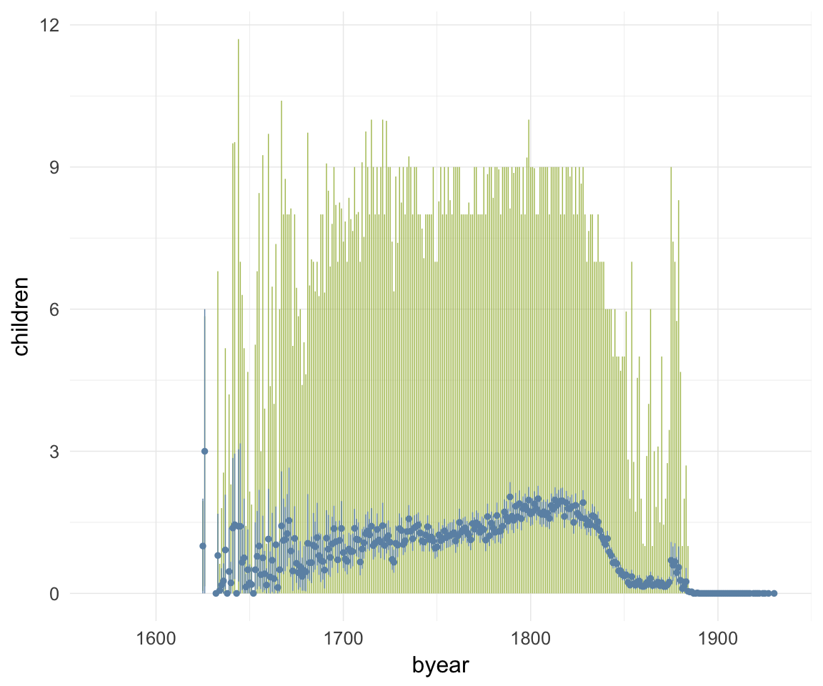
ggplot(data=krmh, aes(x = byear, y = survive1y)) +
    geom_pointrange(stat = "summary", fun.data = "mean_cl_boot", colour = "#aec05d") +

    desc_theme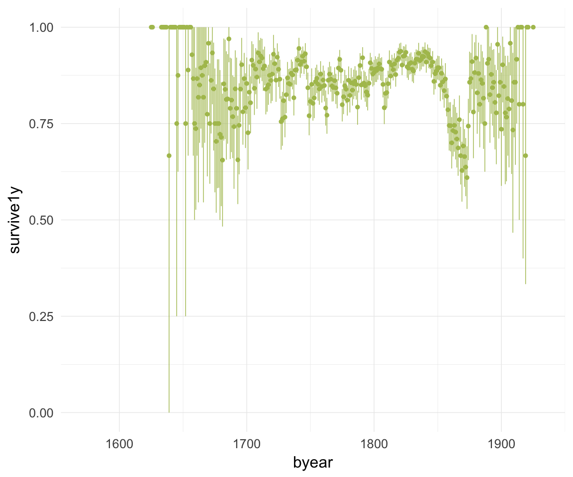
ggplot(data=krmh, aes(x = byear, y = surviveR)) +
    geom_pointrange(stat = "summary", fun.data = "mean_cl_boot", colour = "#aec05d") +

    desc_theme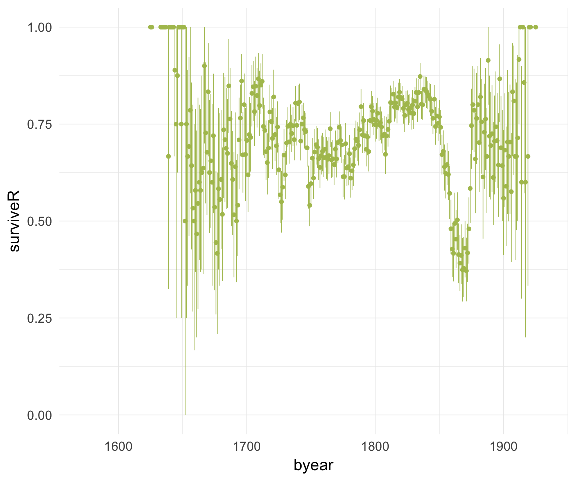
ggplot(data=krmh, aes(x = children, y = grandchildren)) +
    geom_jitter(colour = "#aec05d", alpha = I(0.1)) +
    geom_pointrange(stat = "summary", fun.data = "median_hilow", colour = "#6c92b2") +
    geom_smooth(method = "glm", formula = y ~ poly(x,3), colour = "#6e85b0") +
    desc_theme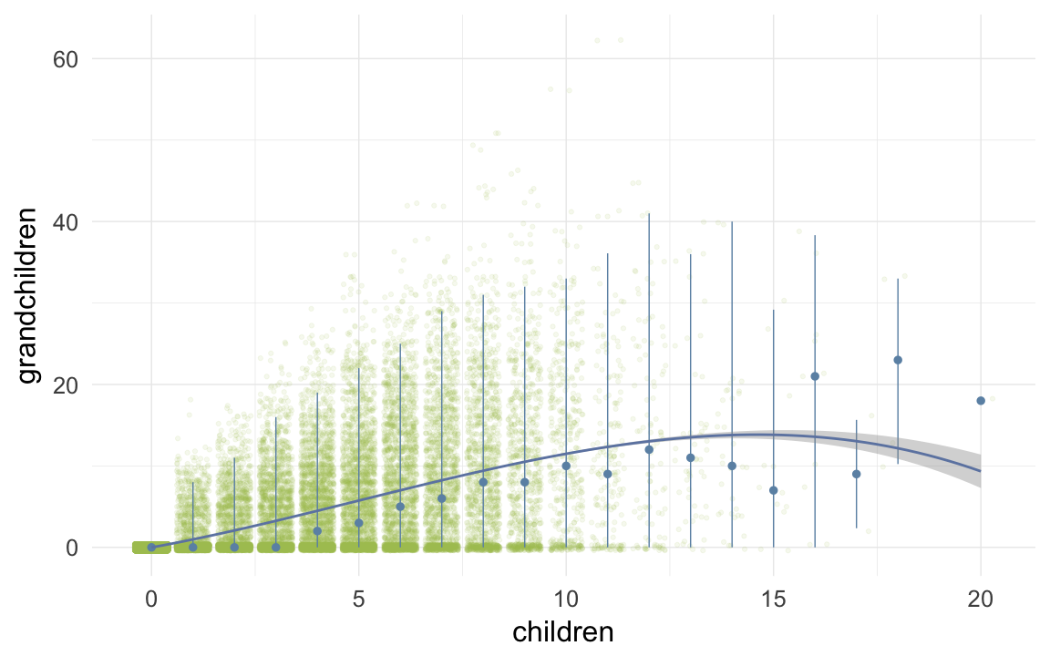
ggplot(data=krmh, aes(x = children, y = children.surviving5y)) +
    geom_jitter(colour = "#aec05d", alpha = I(0.1)) +
    geom_pointrange(stat = "summary", fun.data = "median_hilow", colour = "#6c92b2") +
    geom_smooth(method = "glm", formula = y ~ poly(x,3), colour = "#6e85b0") +
    desc_theme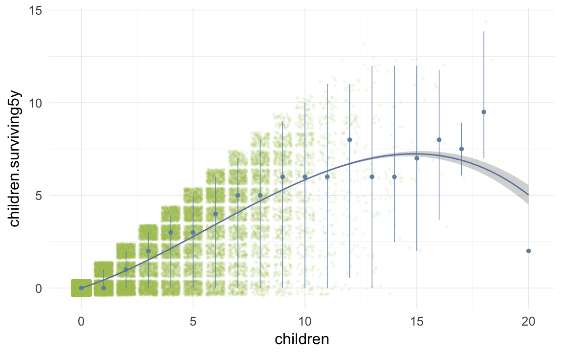
ggplot(data=krmh, aes(x = round(age), y = children)) +
    geom_jitter(colour = "#aec05d", alpha = I(0.1)) +
    geom_pointrange(stat = "summary", fun.data = "mean_cl_boot", colour = "#6c92b2") +
    geom_smooth(colour = "#6e85b0") +
    xlab("Age") +
    ylab("Number of children") +
    desc_theme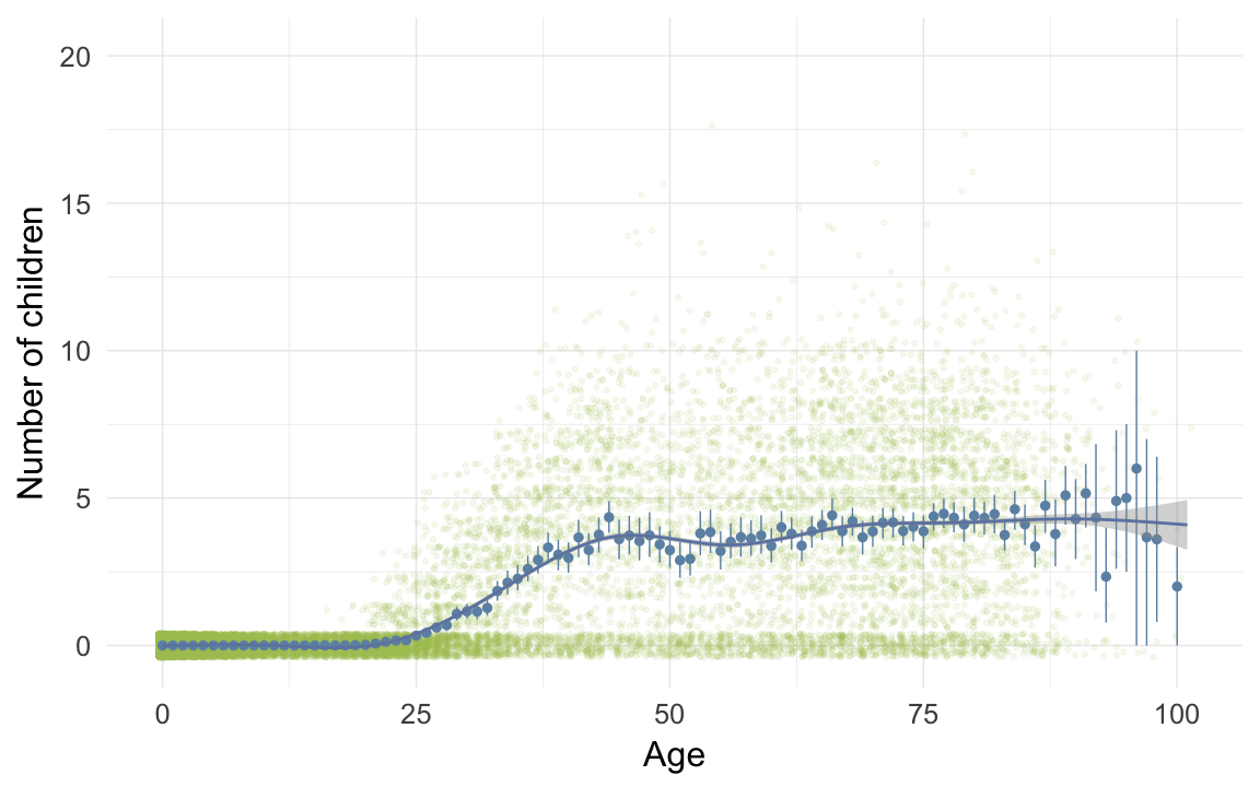
ggplot(data=krmh[children>0,], aes(x = round(age), y = children)) +
    geom_jitter(colour = "#aec05d", alpha = I(0.1)) +
    geom_pointrange(stat = "summary", fun.data = "mean_cl_boot", colour = "#6c92b2") +
    geom_smooth(colour = "#6e85b0") +
    xlab("Age") +
    ylab("Number of children") +
    desc_theme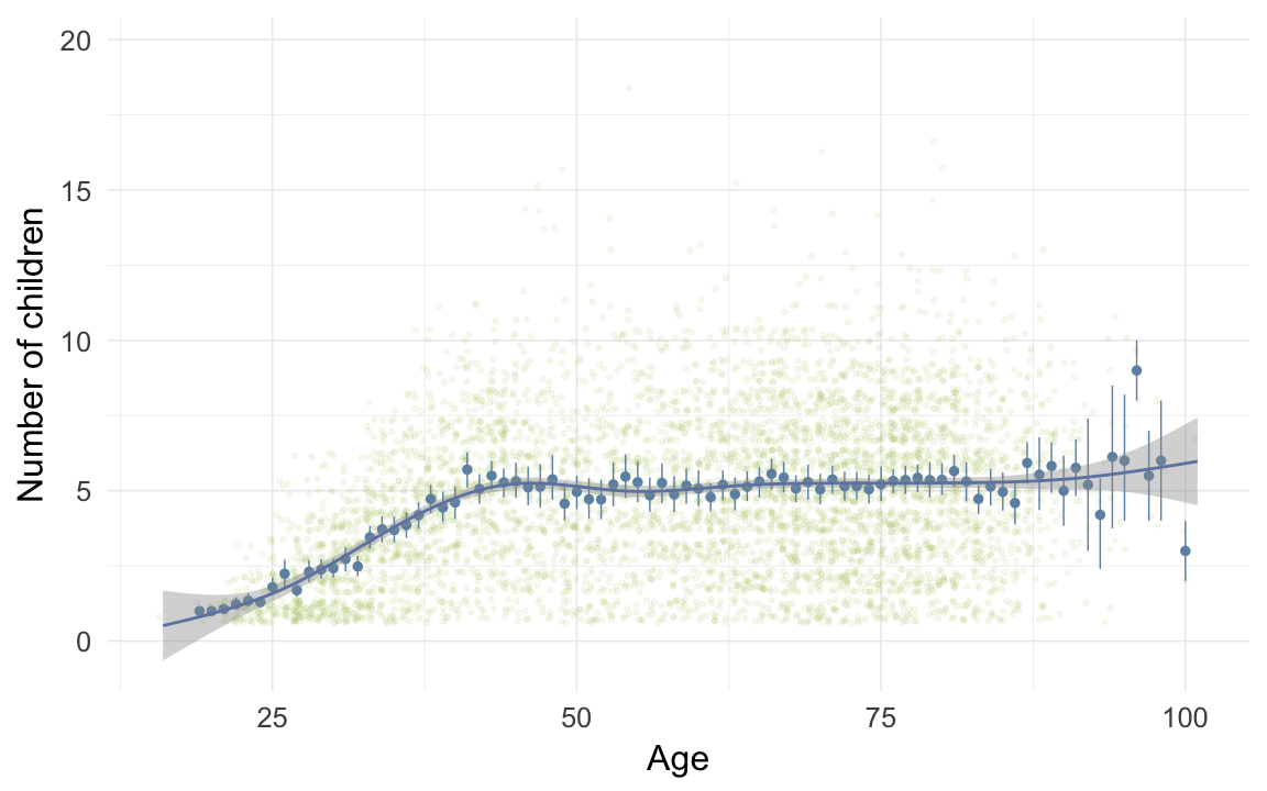
plot_zero_infl(krmh[ spouses > 0, ]$children)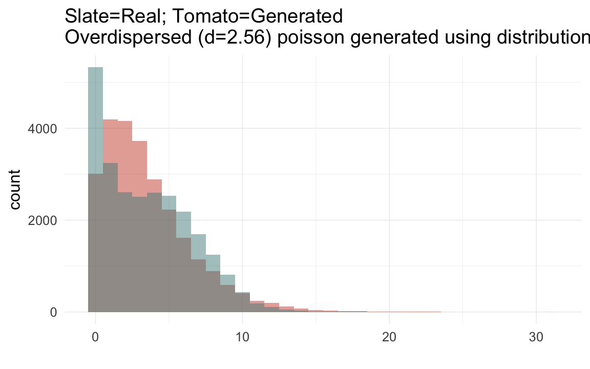
ggplot(data=krmh, aes(x = paternalage.factor, y = survive1y)) +
    geom_pointrange(stat = "summary", fun.data = "mean_cl_boot", colour = "#aec05d") +
    desc_theme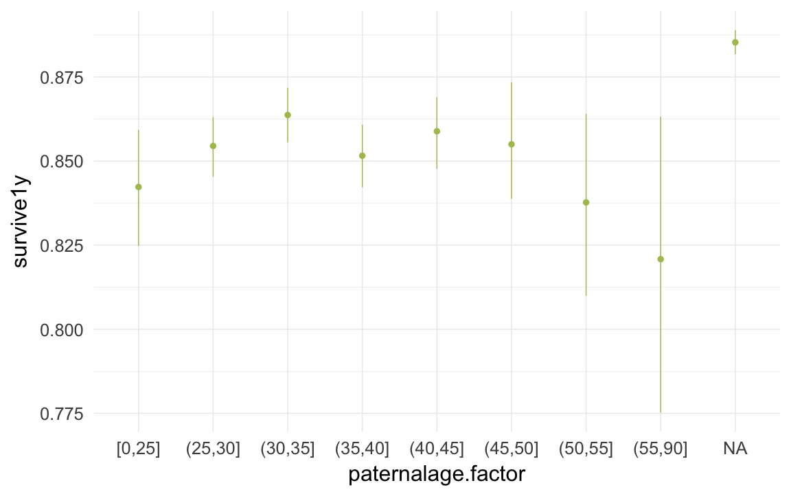
ggplot(data=krmh[spouses > 0, ], aes(x = paternalage.factor, y = children)) +
    geom_pointrange(stat = "summary", fun.data = "mean_cl_boot", colour = "#aec05d") +
    desc_theme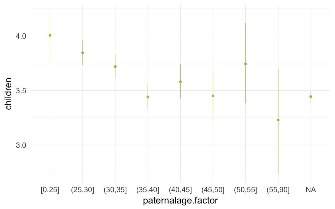
Opportunities for selection
krmh.1$birth.decade = round(krmh.1$byear/5)*5


episodes = krmh.1 %>%
    filter(!is.na(male) | !is.na(survive1y) | !is.na(ever_married)) %>%
    group_by(birth.decade) %>%
    summarise(
        "Population size" = as.numeric(length(idIndividu)),
        "0. Number of children" = ifelse(between(birth.decade, 1655,1840), cva(children), NA_real_ ),
        "1. Surviving first year" = ifelse(between(birth.decade, 1655, 1870),cva_bin(survive1y), NA_real_ ),
        "2. Surviving to 15" = ifelse(between(birth.decade, 1655,1840), cva_bin(surviveR[survive1y==T]), NA_real_ ),
        "3. Ever married" = ifelse(between(birth.decade, 1655,1830), cva_bin(ever_married[surviveR==1]), NA_real_ ),
        "4. Number of children" = ifelse(between(birth.decade, 1655,1840), cva(children[ever_married==1]), NA_real_ ),
        "5. Grandchildren" = ifelse(between(birth.decade, 1655,1800), cva(grandchildren[children>0]), NA_real_ )
        ) %>%
    data.table()
data.frame(episodes[order(birth.decade), ])| birth.decade | Population.size | X0..Number.of.children | X1..Surviving.first.year | X2..Surviving.to.15 | X3..Ever.married | X4..Number.of.children | X5..Grandchildren |
|---|---|---|---|---|---|---|---|
| 1720 | 26 | 1.775 | 0.3612 | 0.4588 | 1.054 | 0.6663 | 1.152 |
| 1725 | 84 | 2.404 | 0.2516 | 0.6409 | 1.453 | 0.681 | 0.8613 |
| 1730 | 126 | 1.899 | 0.5222 | 0.4873 | 0.9753 | 0.7081 | 1.091 |
| 1735 | 182 | 1.74 | 0.3708 | 0.4097 | 1.052 | 0.6631 | 1.146 |
| 1740 | 203 | 1.784 | 0.3119 | 0.4044 | 1.157 | 0.6342 | 0.9587 |
| 1745 | 270 | 1.731 | 0.2828 | 0.5373 | 1.031 | 0.6257 | 1.066 |
| 1750 | 286 | 1.97 | 0.4934 | 0.5405 | 1.023 | 0.6969 | 0.9427 |
| 1755 | 359 | 2.034 | 0.439 | 0.5505 | 1.067 | 0.7394 | 1.149 |
| 1760 | 484 | 1.877 | 0.4214 | 0.5333 | 1.065 | 0.6344 | 0.8095 |
| 1765 | 597 | 1.926 | 0.4075 | 0.5261 | 1.059 | 0.7015 | 0.989 |
| 1770 | 637 | 1.742 | 0.4238 | 0.4884 | 0.9079 | 0.7171 | 0.9014 |
| 1775 | 674 | 1.718 | 0.3951 | 0.4957 | 0.8944 | 0.7247 | 0.9555 |
| 1780 | 684 | 1.689 | 0.4378 | 0.5948 | 0.8061 | 0.669 | 0.9041 |
| 1785 | 638 | 1.628 | 0.4157 | 0.4804 | 0.825 | 0.7102 | 0.8965 |
| 1790 | 730 | 1.581 | 0.3702 | 0.4547 | 0.83 | 0.714 | 0.9086 |
| 1795 | 831 | 1.521 | 0.4168 | 0.4449 | 0.7729 | 0.6896 | 0.9737 |
| 1800 | 924 | 1.51 | 0.36 | 0.4347 | 0.7674 | 0.733 | 1.013 |
| 1805 | 963 | 1.496 | 0.3646 | 0.4778 | 0.7357 | 0.7142 | NA |
| 1810 | 909 | 1.55 | 0.4534 | 0.4155 | 0.7412 | 0.744 | NA |
| 1815 | 1016 | 1.293 | 0.3537 | 0.3549 | 0.6187 | 0.7249 | NA |
| 1820 | 1044 | 1.391 | 0.3034 | 0.402 | 0.6643 | 0.7775 | NA |
| 1825 | 1056 | 1.448 | 0.3162 | 0.4371 | 0.6667 | 0.7979 | NA |
| 1830 | 910 | 1.482 | 0.367 | 0.3839 | 0.7003 | 0.8045 | NA |
| 1835 | 401 | 1.332 | 0.3375 | 0.3875 | NA | 0.7366 | NA |
save(episodes, file = "coefs/krmh_episodes.rdata")
# krmh.1 = merge(krmh.1, episodes, by = "birth.decade", all.x = T)(episodes.plot = ggplot(melt(episodes,id.vars=c('birth.decade'), na.rm = T)) + geom_line(aes(x=birth.decade, y=value)) + facet_wrap(~ variable,scales='free_y',ncol = 1)) + mymin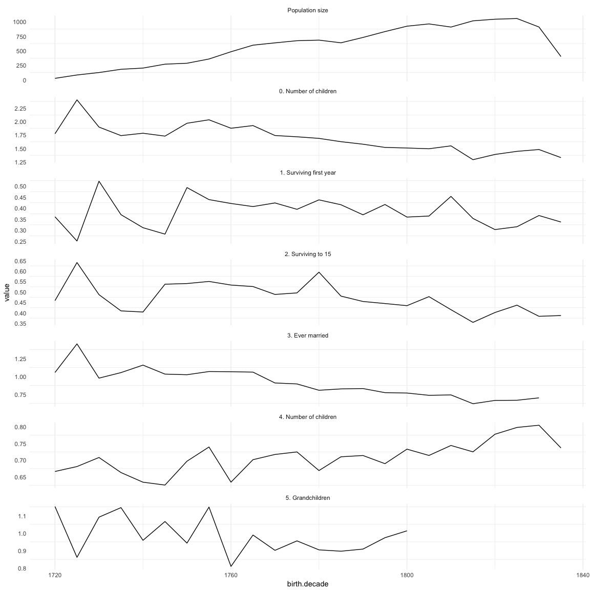
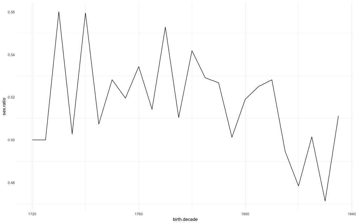
Sex ratio
(sex.ratio = krmh.1 %>%
    filter(!is.na(male), byear > 1720) %>%
    mutate(male = as.numeric(as.character(male))) %>%
    group_by(birth.decade) %>%
    summarise(sex.ratio = sum(male)/length(male)) %>%
    data.frame()
)| birth.decade | sex.ratio |
|---|---|
| 1760 | 0.5343 |
| 1765 | 0.5143 |
| 1770 | 0.5528 |
| 1775 | 0.5105 |
| 1790 | 0.5267 |
| 1795 | 0.5012 |
| 1800 | 0.519 |
| 1805 | 0.525 |
| 1810 | 0.5281 |
| 1815 | 0.4946 |
| 1820 | 0.4784 |
| 1780 | 0.5417 |
| 1785 | 0.529 |
| 1825 | 0.5014 |
| 1830 | 0.4714 |
| 1835 | 0.5112 |
| 1755 | 0.5196 |
| 1740 | 0.5594 |
| 1745 | 0.5074 |
| 1750 | 0.5282 |
| 1735 | 0.5028 |
| 1730 | 0.56 |
| 1725 | 0.5 |
| 1720 | 0.5 |
ggplot(na.omit(sex.ratio)) + geom_line(aes(x=birth.decade, y=sex.ratio)) + mymin