RPQA Quebec descriptives
Loading details
source("0__helpers.R")

opts_chunk$set(render = pander_handler, cache=F,tidy=FALSE,autodep=TRUE,dev='png',fig.width=12,fig.height=7.5, warning = F, message = F)
load("rpqa.rdata")
rpqa = data.table(rpqa); rpqa.1 = data.table(rpqa.1)
desc_theme = theme_minimal(base_size = 24) + theme( axis.line.y = element_blank(), axis.line.x = element_line(size = 1, color ="black"))
update_geom_defaults("bar",   list(fill = "#6c92b2", alpha = 1/2))

demo_trends = aggDemoTrends(rpqa)

mymin = theme_minimal() +theme(panel.grid.major.y =element_blank(),panel.grid.major.x = element_line(colour="#eeeeee"))

rpqa[, paternalage := 10 * paternalage]
rpqa[, maternalage := 10 * maternalage]
rpqa[, age := 10 * age]
rpqa[, age_at_1st_child := 10 * age_at_1st_child]
rpqa[, age_at_last_child := 10 * age_at_last_child]
rpqa[, byear := year(bdate)]
rpqa.1[, paternalage := 10 * paternalage]
rpqa.1[, maternalage := 10 * maternalage]
rpqa.1[, age := 10 * age]
rpqa.1[, age_at_1st_child := 10 * age_at_1st_child]
rpqa.1[, age_at_last_child := 10 * age_at_last_child]
rpqa.1[, byear := year(bdate)]
Variable descriptives
The following statistics refer to all births. This means that e.g. the percentage of ever married people includes some who died before they had a chance at marriage.
Whole population (N = 459591)
descriptives = psych::describe(rpqa[, list(
    paternalage, maternalage, nr.siblings, dependent_sibs_f5y, age, spouses, children, grandchildren, byear, byear.Father, age_at_1st_child, age_at_last_child  )])
round(data.frame(descriptives)[,2:12],2)| n | mean | sd | median | trimmed | mad | min | max | range | skew | kurtosis | |
|---|---|---|---|---|---|---|---|---|---|---|---|
| paternalage | 396965 | 35.64 | 8.43 | 34.53 | 35.05 | 8.54 | 14.84 | 85.44 | 70.61 | 0.7 | 0.43 |
| maternalage | 399603 | 29.71 | 6.64 | 29.2 | 29.5 | 7.49 | 9.95 | 69.27 | 59.32 | 0.25 | -0.71 |
| nr.siblings | 427016 | 7.93 | 4.13 | 8 | 7.93 | 4.45 | 0 | 22 | 22 | 0.03 | -0.52 |
| dependent_sibs_f5y | 459591 | 2098 | 7640 | 3 | 2.95 | 1.48 | 0 | 31552 | 31552 | 3.42 | 9.83 |
| age | 239638 | 25.48 | 31.29 | 3.19 | 21.56 | 4.72 | 0 | 112.1 | 112.1 | 0.76 | -1.08 |
| spouses | 459591 | 0.32 | 0.55 | 0 | 0.22 | 0 | 0 | 6 | 6 | 1.73 | 3.08 |
| children | 459591 | 1.86 | 3.79 | 0 | 0.86 | 0 | 0 | 31 | 31 | 2.19 | 4.13 |
| grandchildren | 459591 | 3.56 | 12.25 | 0 | 0.34 | 0 | 0 | 195 | 195 | 4.81 | 27.45 |
| byear | 427685 | 1761 | 33.64 | 1770 | 1765 | 29.65 | 1583 | 1799 | 216 | -1.28 | 1.56 |
| byear.Father | 401758 | 1728 | 31.89 | 1735 | 1731 | 28.17 | 1583 | 1782 | 199 | -1.03 | 0.74 |
| age_at_1st_child | 110119 | 25.36 | 5.64 | 24.47 | 24.8 | 4.87 | 9.95 | 81.2 | 71.25 | 1.35 | 3.83 |
| age_at_last_child | 110119 | 37.5 | 9.14 | 38.1 | 37.33 | 8.98 | 13.84 | 85.44 | 71.6 | 0.24 | 0.16 |
describeBin(rpqa[, list(survive1y, surviveR, ever_married)])| n | mean | sd | |
|---|---|---|---|
| survive1y | 303094 | 0.68 | 0.22 |
| surviveR | 303094 | 0.55 | 0.25 |
| ever_married | 459591 | 0.28 | 0.2 |
pander(xtabs(~ paternal_loss, rpqa), caption = "Paternal loss at age")| later | [0,1] | (1,5] | (5,10] | (10,15] | (15,20] | (20,25] | (25,30] | (30,35] | (35,40] | (40,45] | unclear |
|---|---|---|---|---|---|---|---|---|---|---|---|
| 67685 | 5903 | 12520 | 17507 | 21294 | 26344 | 32911 | 36337 | 37820 | 37750 | 28036 | 135484 |
pander(xtabs(~ maternal_loss, rpqa), caption = "Maternal loss at age")| later | [0,1] | (1,5] | (5,10] | (10,15] | (15,20] | (20,25] | (25,30] | (30,35] | (35,40] | (40,45] | unclear |
|---|---|---|---|---|---|---|---|---|---|---|---|
| 96785 | 8922 | 17870 | 19592 | 18031 | 18390 | 21247 | 25498 | 29276 | 32748 | 27878 | 143354 |
included sample (N = 79895)
descriptives = psych::describe(rpqa.1[, list(
    paternalage, maternalage, nr.siblings, dependent_sibs_f5y, age, spouses, children, grandchildren, byear, byear.Father, age_at_1st_child, age_at_last_child  )])
round(data.frame(descriptives)[,2:12],2)| n | mean | sd | median | trimmed | mad | min | max | range | skew | kurtosis | |
|---|---|---|---|---|---|---|---|---|---|---|---|
| paternalage | 70035 | 36.58 | 8.68 | 35.43 | 35.97 | 8.83 | 16.77 | 78.92 | 62.15 | 0.65 | 0.2 |
| maternalage | 70776 | 29.33 | 6.69 | 28.79 | 29.11 | 7.5 | 12.01 | 53.03 | 41.02 | 0.27 | -0.69 |
| nr.siblings | 76485 | 8.17 | 4.15 | 9 | 8.28 | 4.45 | 0 | 22 | 22 | -0.18 | -0.42 |
| dependent_sibs_f5y | 79895 | 1036 | 4895 | 3 | 2.97 | 1.48 | 0 | 24408 | 24408 | 4.52 | 18.48 |
| age | 66097 | 39.14 | 30.92 | 39.33 | 38.38 | 47.46 | 0 | 112.1 | 112.1 | 0.03 | -1.5 |
| spouses | 79895 | 0.62 | 0.7 | 1 | 0.52 | 1.48 | 0 | 6 | 6 | 0.94 | 0.84 |
| children | 79895 | 3.91 | 5.13 | 0 | 3.1 | 0 | 0 | 31 | 31 | 1.03 | -0.11 |
| grandchildren | 79895 | 12.52 | 21.61 | 0 | 7.45 | 0 | 0 | 174 | 174 | 2.11 | 4.62 |
| byear | 79895 | 1715 | 18.7 | 1719 | 1716 | 19.27 | 1670 | 1739 | 69 | -0.64 | -0.62 |
| byear.Father | 70035 | 1678 | 21.08 | 1681 | 1680 | 22.24 | 1599 | 1720 | 121 | -0.5 | -0.59 |
| age_at_1st_child | 37445 | 26.29 | 6.12 | 25.3 | 25.66 | 5.22 | 13.01 | 81.2 | 68.19 | 1.41 | 4.02 |
| age_at_last_child | 37445 | 40.66 | 8.85 | 41.16 | 40.62 | 7.14 | 13.84 | 85.44 | 71.6 | 0.14 | 0.67 |
describeBin(rpqa.1[, list(survive1y, surviveR, ever_married)])| n | mean | sd | |
|---|---|---|---|
| survive1y | 71311 | 0.81 | 0.15 |
| surviveR | 71311 | 0.71 | 0.21 |
| ever_married | 79895 | 0.51 | 0.25 |
pander(xtabs(~ paternal_loss, rpqa.1), caption = "Paternal loss at age")| later | [0,1] | (1,5] | (5,10] | (10,15] | (15,20] | (20,25] | (25,30] | (30,35] | (35,40] | (40,45] | unclear |
|---|---|---|---|---|---|---|---|---|---|---|---|
| 9638 | 1379 | 2763 | 4010 | 4818 | 5691 | 6705 | 7161 | 7203 | 6986 | 4865 | 18676 |
pander(xtabs(~ maternal_loss, rpqa.1), caption = "Maternal loss at age")| later | [0,1] | (1,5] | (5,10] | (10,15] | (15,20] | (20,25] | (25,30] | (30,35] | (35,40] | (40,45] | unclear |
|---|---|---|---|---|---|---|---|---|---|---|---|
| 19332 | 1468 | 3018 | 3800 | 3934 | 4044 | 4350 | 5017 | 6152 | 7018 | 5699 | 16063 |
Number of families with varying numbers of siblings available for comparison
crosstabs(rpqa[!duplicated(idParents), ]$nr.siblings)| 0 | 1 | 2 | 3 | 4 | 5 | 6 | 7 | 8 | 9 | 10 | 11 | 12 | 13 | 14 | 15 | 16 | 17 | 18 | 19 | 20 | 21 | 22 | NA |
|---|---|---|---|---|---|---|---|---|---|---|---|---|---|---|---|---|---|---|---|---|---|---|---|
| 17055 | 6596 | 6005 | 5479 | 5156 | 4782 | 4544 | 4330 | 4205 | 4005 | 3527 | 2819 | 2076 | 1494 | 990 | 623 | 342 | 205 | 90 | 45 | 16 | 4 | 6 | 1 |
qplot(rpqa[!duplicated(idParents), ]$nr.siblings, binwidth = 1) + xlab("Number of siblings per family") + desc_theme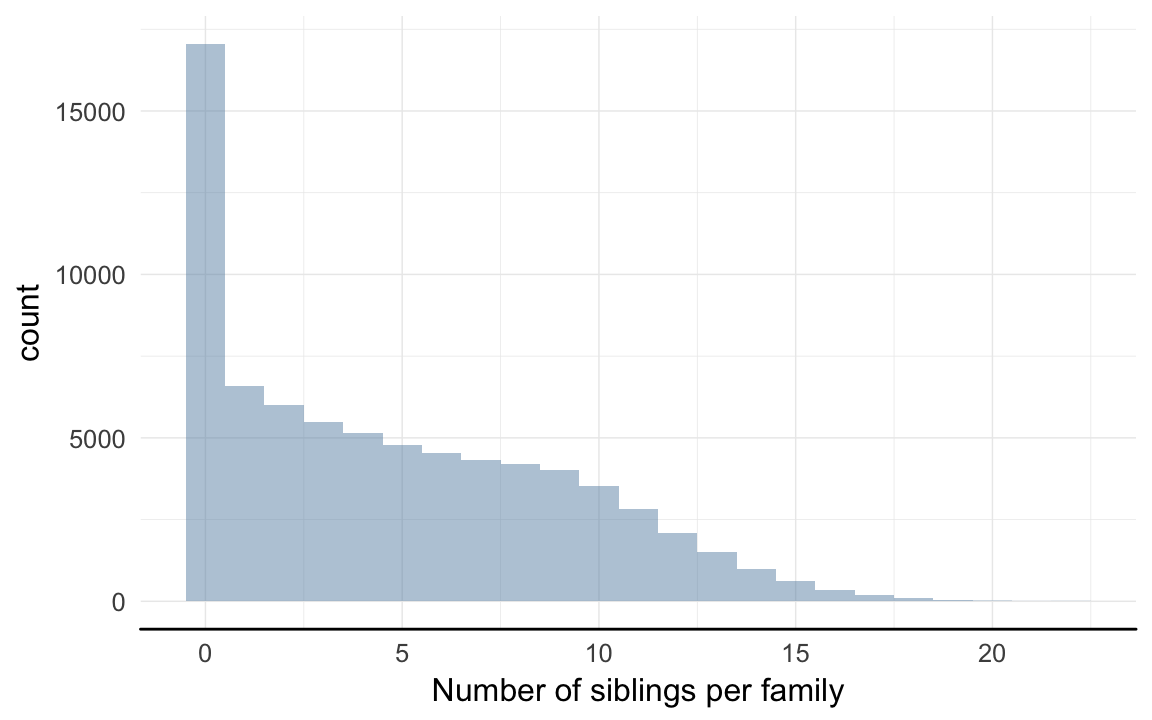
Missingness patterns
The first table shows the number of missings per variable, the second table, using the indexes from the first, shows missings in which variables tend to occur together. Most variables of interest in this study are derived from these dates and so these patterns can show many cases did not have the data to calculate e.g. paternal loss (those lacking either the father’s death date, the anchor’s birth date or both).
pander_escape(missingness_patterns(rpqa[, list(
    bdate, ddate, bdate.Father, ddate.Father, bdate.Mother, ddate.Mother
    )]))
## index col missings
## 1 ddate 214777
## 2 ddate.Mother 139108
## 3 ddate.Father 131403
## 4 bdate.Father 57833
## 5 bdate.Mother 54978
## 6 bdate 31906| Pattern | Freq | Culprit |
|---|---|---|
| ___________ | 166503 | _ |
| 1__________ | 102985 | ddate |
| 1_2________ | 28009 | |
| 1_2_3_4_5_6 | 24048 | |
| 1_2_3______ | 22747 | |
| ____3______ | 21009 | ddate.Father |
| __2________ | 19750 | ddate.Mother |
| 1___3______ | 17574 | |
| __2_3_4_5__ | 13719 | |
| __2_3______ | 11033 | |
| 1_2_3_4_5__ | 6846 | |
| __2_3_4_5_6 | 2697 | |
| ____3_4____ | 2465 | |
| 1_2_3_4____ | 2198 | |
| 1_2_____5__ | 2155 | |
| 1___3_4____ | 2129 | |
| 1_________6 | 1821 | |
| 1_2_3___5__ | 1819 | |
| __________6 | 1678 | bdate |
| ______4____ | 1131 | bdate.Father |
| __2_3_4____ | 1068 | |
| ________5__ | 985 | bdate.Mother |
| __2_____5__ | 976 | |
| __2_3___5__ | 697 | |
| 1_____4____ | 648 | |
| 1_______5__ | 532 | |
| __2_______6 | 251 | |
| ____3_____6 | 249 | |
| 1_2___4____ | 216 | |
| 1___3_____6 | 212 | |
| 1_2_______6 | 181 | |
| __2_3_____6 | 154 | |
| 1___3_4___6 | 146 | |
| __2___4____ | 138 | |
| 1_2_3_____6 | 114 | |
| ____3___5__ | 96 | |
| 1___3___5__ | 95 | |
| 1_2_3_4___6 | 67 | |
| ____3_4___6 | 63 | |
| 1_2_____5_6 | 52 | |
| 1___3_4_5__ | 42 | |
| 1_2___4_5__ | 39 | |
| 1_2_3___5_6 | 33 | |
| ____3_4_5__ | 33 | |
| __2___4_5__ | 30 | |
| __2_3_4___6 | 28 | |
| 1_____4___6 | 18 | |
| ______4___6 | 17 | |
| 1_______5_6 | 14 | |
| 1_____4_5__ | 13 | |
| __2_____5_6 | 12 | |
| __2_3___5_6 | 11 | |
| ________5_6 | 9 | |
| 1_2___4_5_6 | 8 | |
| 1_2___4___6 | 8 | |
| 1___3_4_5_6 | 8 | |
| ______4_5__ | 5 | |
| __2___4___6 | 3 | |
| ____3___5_6 | 2 | |
| __2___4_5_6 | 1 | |
| ____3_4_5_6 | 1 |
Reproductive timing
ggplot(data = demo_trends) +
    geom_line(aes(x= Year, y = first, linetype = "first", colour = Parent),  size = 1) +
  geom_line(aes(x = Year, y = all, linetype = "all", colour = Parent), size = 1) +
    geom_line(aes(x= Year, y = last, linetype = "last", colour = Parent),size = 1) +
    scale_colour_manual(values = c(Father = "#6c92b2", Mother = "#aec05d")) +
    scale_linetype_manual("Birth", breaks = c("last", "all","first"), values = c( "solid","dashed", "dotted")) +
    scale_y_continuous("Parental age at birth") +
    xlim(1650,NA) +
        geom_text(aes(x = Year, y = all + 0.5,
                                    label = ifelse(Year %% 15 == 0, round(all), NA))) +
    facet_wrap(~ Parent) +
    desc_theme + theme(legend.position = c(1,1),
  legend.justification = c(1,1),
  legend.box = "horizontal",
  panel.margin = unit(2, "lines"))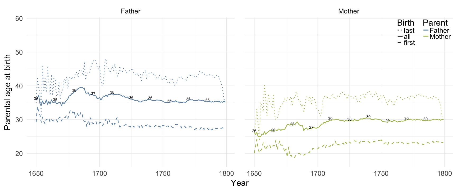
Correlations between variables
round(cor(rpqa[, list(
    paternalage, maternalage, birthorder, nr.siblings, children, grandchildren, byear, byear.Father, age_at_1st_child, age_at_last_child
)], use = "pairwise.complete.obs"),2)| paternalage | maternalage | birthorder | nr.siblings | children | grandchildren | byear | byear.Father | age_at_1st_child | age_at_last_child | |
|---|---|---|---|---|---|---|---|---|---|---|
| paternalage | 1 | 0.63 | 0.61 | 0.21 | -0.01 | 0.02 | -0.05 | -0.31 | 0.03 | 0.02 |
| maternalage | 0.63 | 1 | 0.72 | 0.17 | -0.04 | -0.04 | 0.05 | -0.11 | 0.01 | -0.02 |
| birthorder | 0.61 | 0.72 | 1 | 0.59 | -0.07 | -0.06 | 0.11 | -0.1 | -0.07 | -0.06 |
| nr.siblings | 0.21 | 0.17 | 0.59 | 1 | 0.02 | -0.02 | -0.02 | -0.18 | -0.11 | -0.1 |
| children | -0.01 | -0.04 | -0.07 | 0.02 | 1 | 0.61 | -0.44 | -0.43 | -0.17 | 0.7 |
| grandchildren | 0.02 | -0.04 | -0.06 | -0.02 | 0.61 | 1 | -0.49 | -0.46 | -0.06 | 0.41 |
| byear | -0.05 | 0.05 | 0.11 | -0.02 | -0.44 | -0.49 | 1 | 0.96 | -0.2 | -0.45 |
| byear.Father | -0.31 | -0.11 | -0.1 | -0.18 | -0.43 | -0.46 | 0.96 | 1 | -0.12 | -0.44 |
| age_at_1st_child | 0.03 | 0.01 | -0.07 | -0.11 | -0.17 | -0.06 | -0.2 | -0.12 | 1 | 0.47 |
| age_at_last_child | 0.02 | -0.02 | -0.06 | -0.1 | 0.7 | 0.41 | -0.45 | -0.44 | 0.47 | 1 |
ggplot(data=rpqa, aes(x = byear, y = paternalage)) +
    geom_linerange(stat = "summary", fun.data = "median_hilow", colour = "#aec05d") +
    geom_pointrange(stat = "summary", fun.data = "mean_cl_boot", colour = "#6c92b2") +
    desc_theme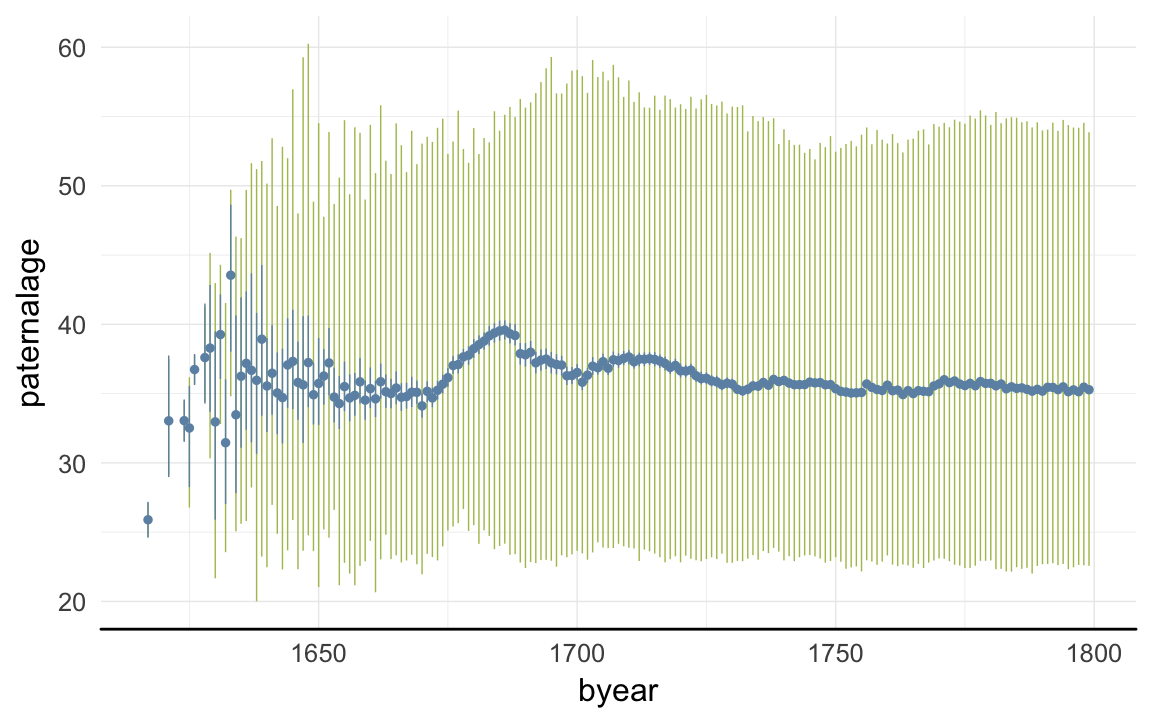
ggplot(data=rpqa, aes(x = byear, y = age_at_1st_child)) +
    geom_linerange(stat = "summary", fun.data = "median_hilow", colour = "#aec05d") +
    geom_pointrange(stat = "summary", fun.data = "mean_cl_boot", colour = "#6c92b2") +
    desc_theme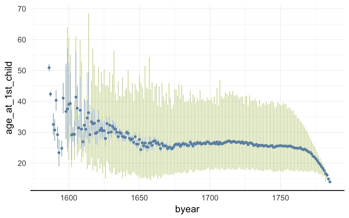
ggplot(data=rpqa, aes(x = byear, y = age_at_last_child)) +
    geom_linerange(stat = "summary", fun.data = "median_hilow", colour = "#aec05d") +
    geom_pointrange(stat = "summary", fun.data = "mean_cl_boot", colour = "#6c92b2") +
    desc_theme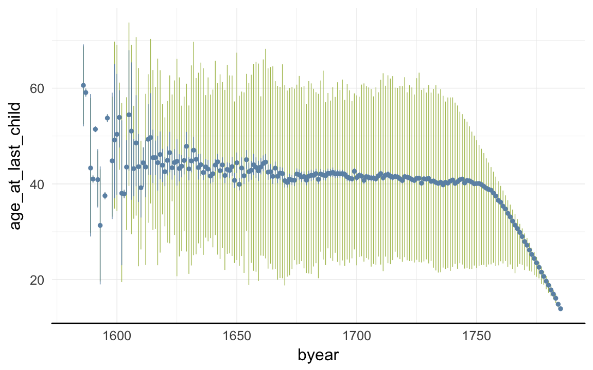
ggplot(data=rpqa, aes(x = byear, y = children)) +
    geom_linerange(stat = "summary", fun.data = "median_hilow", colour = "#aec05d") +
    geom_pointrange(stat = "summary", fun.data = "mean_cl_boot", colour = "#6c92b2") +

    desc_theme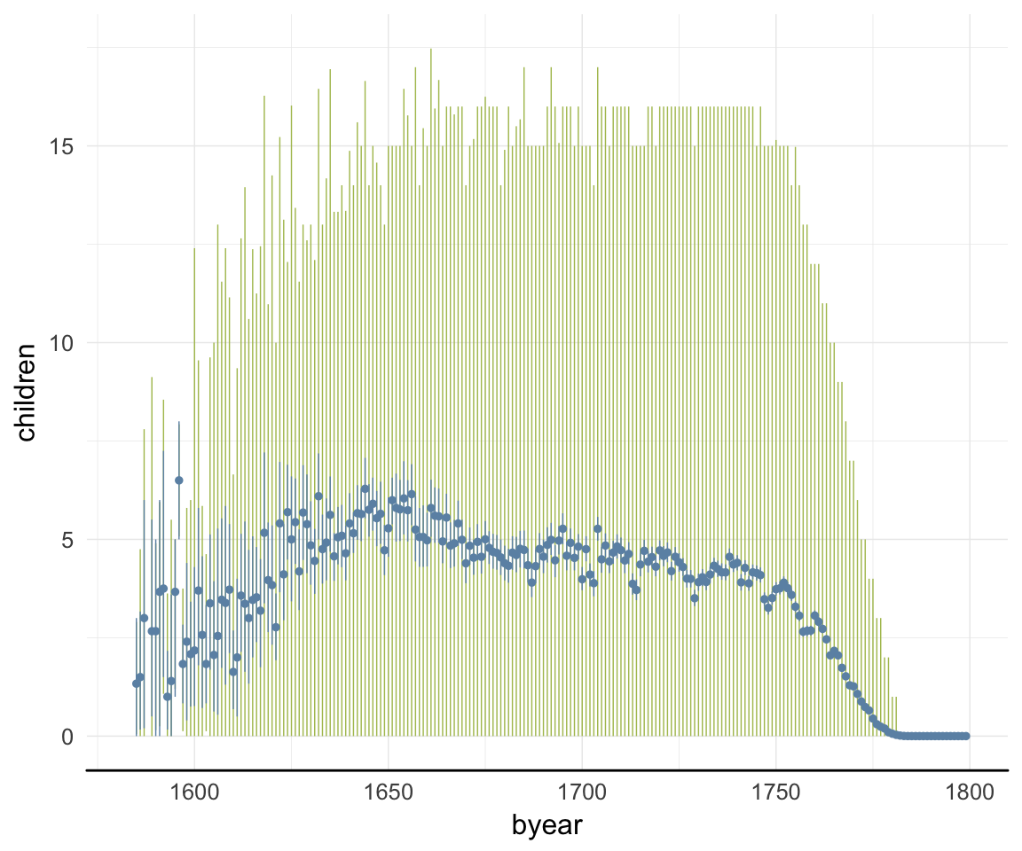
ggplot(data=rpqa, aes(x = byear, y = survive1y)) +
    geom_pointrange(stat = "summary", fun.data = "mean_cl_boot", colour = "#aec05d") +

    desc_theme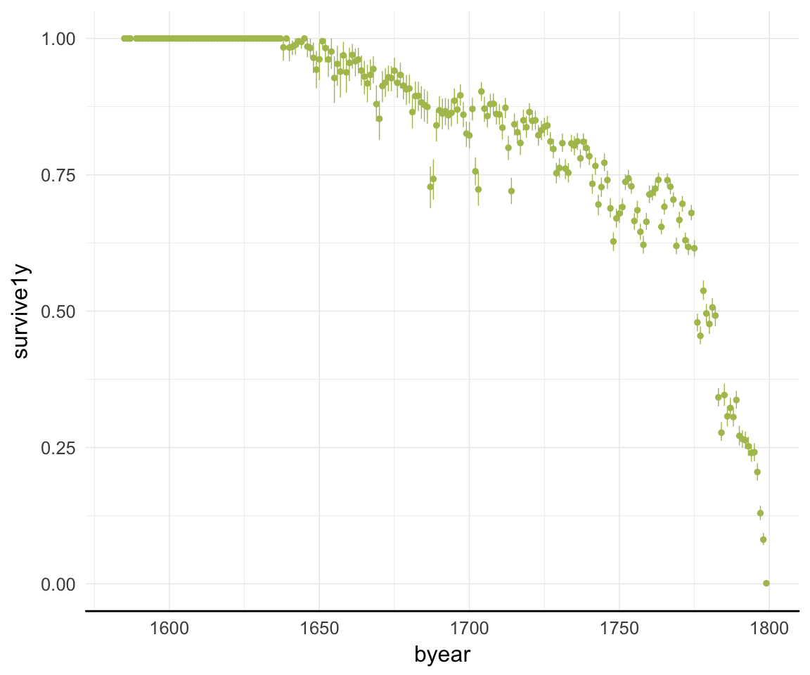
ggplot(data=rpqa, aes(x = byear, y = surviveR)) +
    geom_pointrange(stat = "summary", fun.data = "mean_cl_boot", colour = "#aec05d") +

    desc_theme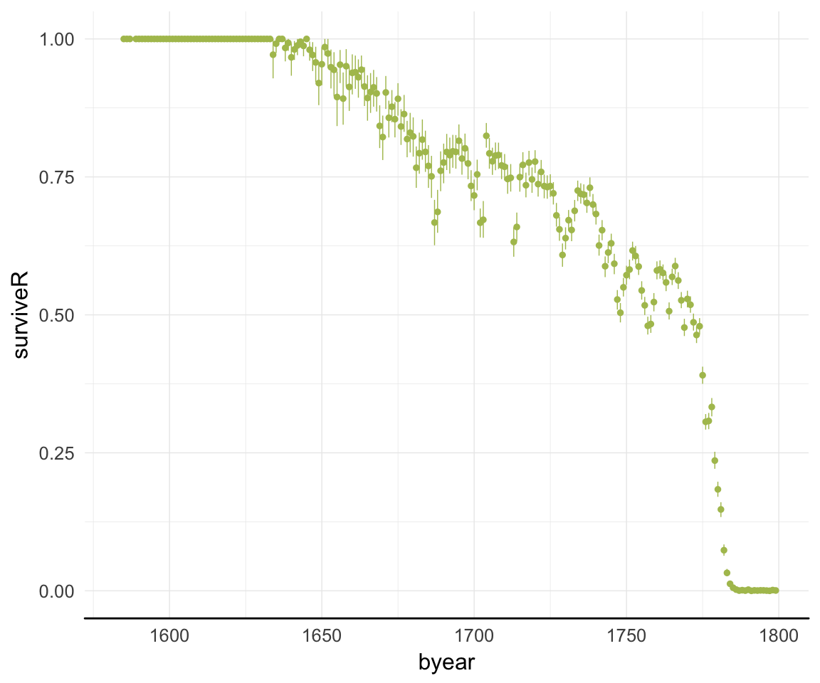
ggplot(data=rpqa, aes(x = children, y = grandchildren)) +
    geom_jitter(colour = "#aec05d", alpha = I(0.1)) +
    geom_pointrange(stat = "summary", fun.data = "median_hilow", colour = "#6c92b2") +
    geom_smooth(method = "glm", formula = y ~ poly(x,3), colour = "#6e85b0") +
    desc_theme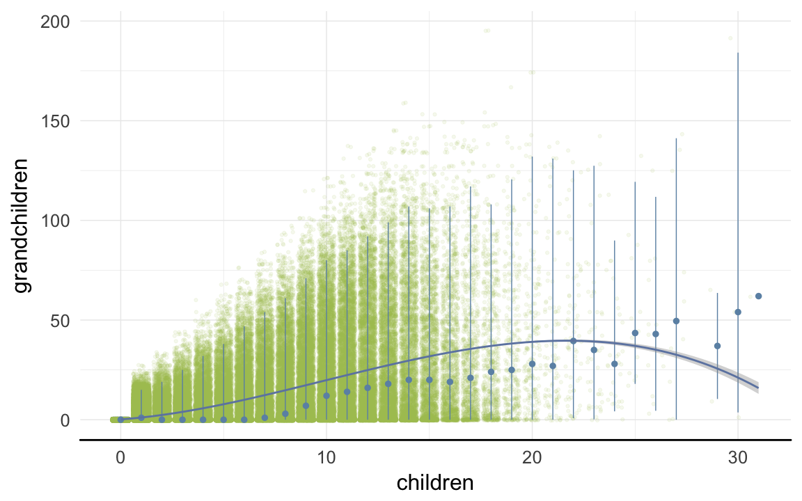
ggplot(data=rpqa, aes(x = children, y = children.surviving5y)) +
    geom_jitter(colour = "#aec05d", alpha = I(0.1)) +
    geom_pointrange(stat = "summary", fun.data = "median_hilow", colour = "#6c92b2") +
    geom_smooth(method = "glm", formula = y ~ poly(x,3), colour = "#6e85b0") +
    desc_theme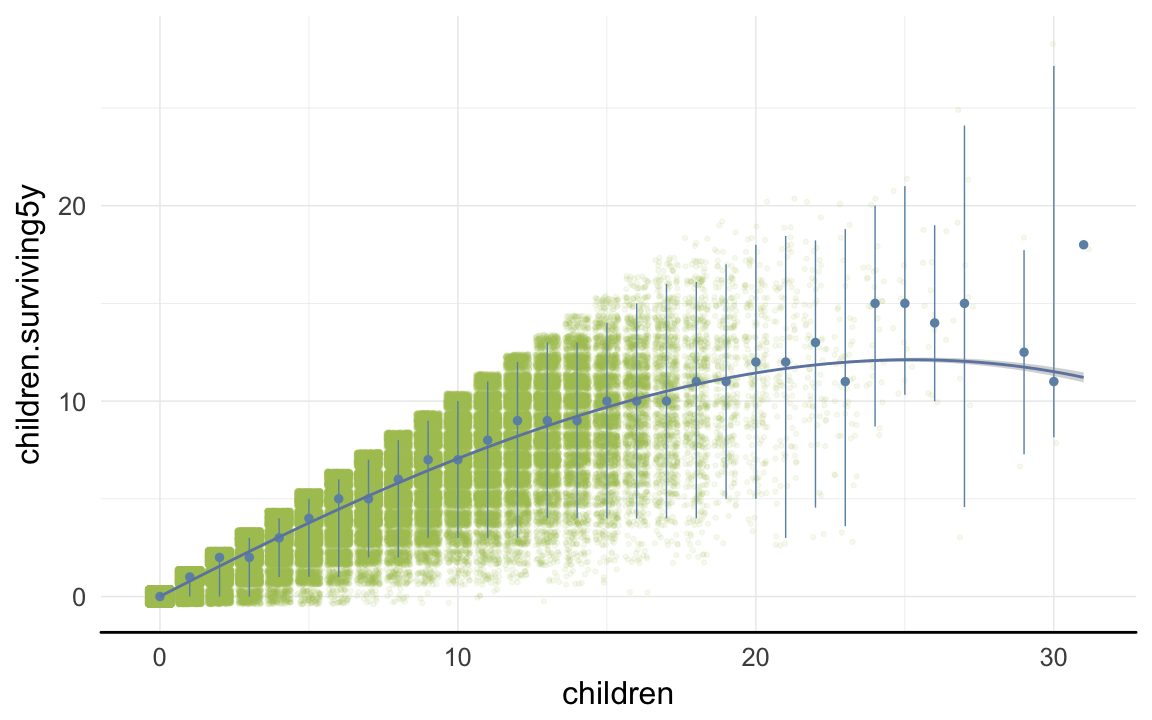
ggplot(data=rpqa, aes(x = round(age), y = children)) +
    geom_jitter(colour = "#aec05d", alpha = I(0.1)) +
    geom_pointrange(stat = "summary", fun.data = "mean_cl_boot", colour = "#6c92b2") +
    geom_smooth(colour = "#6e85b0") +
    xlab("Age") +
    ylab("Number of children") +
    desc_theme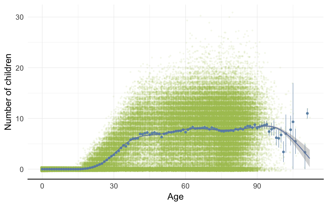
ggplot(data=rpqa[children>0,], aes(x = round(age), y = children)) +
    geom_jitter(colour = "#aec05d", alpha = I(0.1)) +
    geom_pointrange(stat = "summary", fun.data = "mean_cl_boot", colour = "#6c92b2") +
    geom_smooth(colour = "#6e85b0") +
    xlab("Age") +
    ylab("Number of children") +
    desc_theme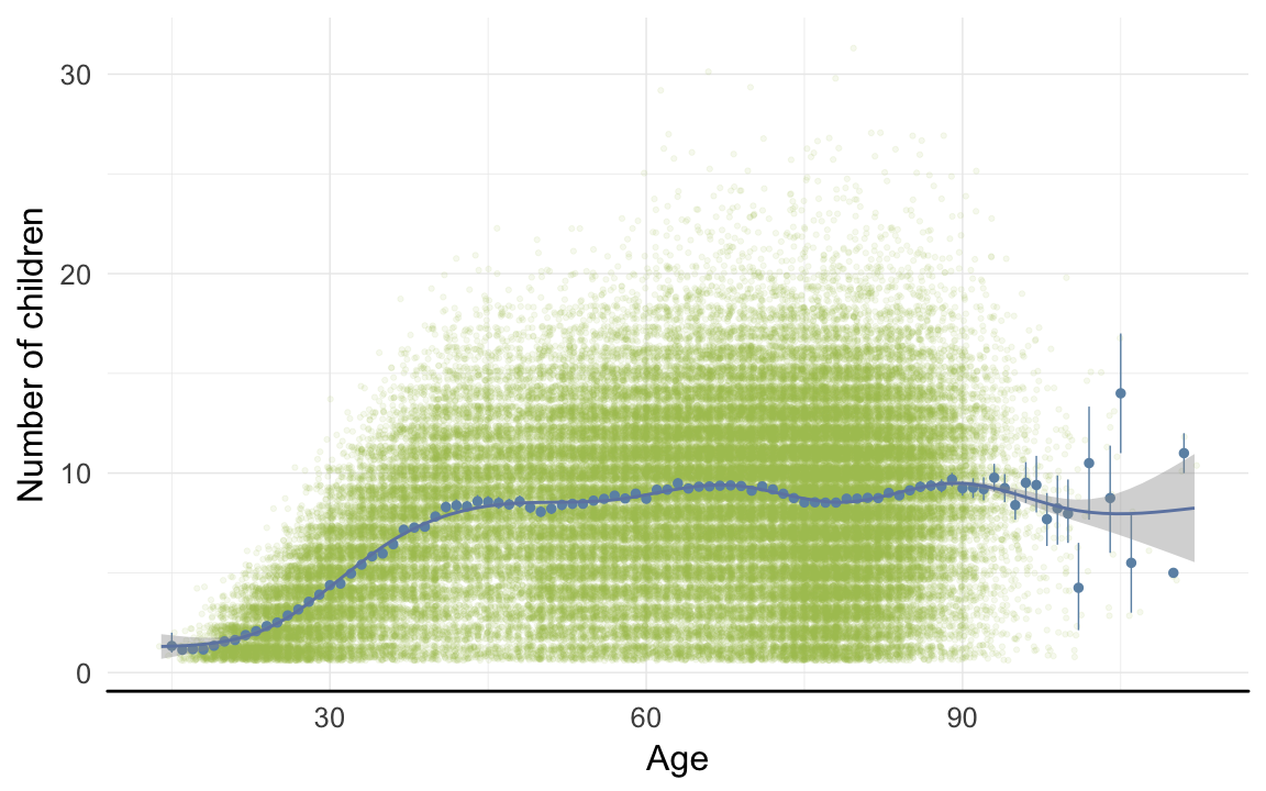
plot_zero_infl(rpqa[ spouses > 0, ]$children)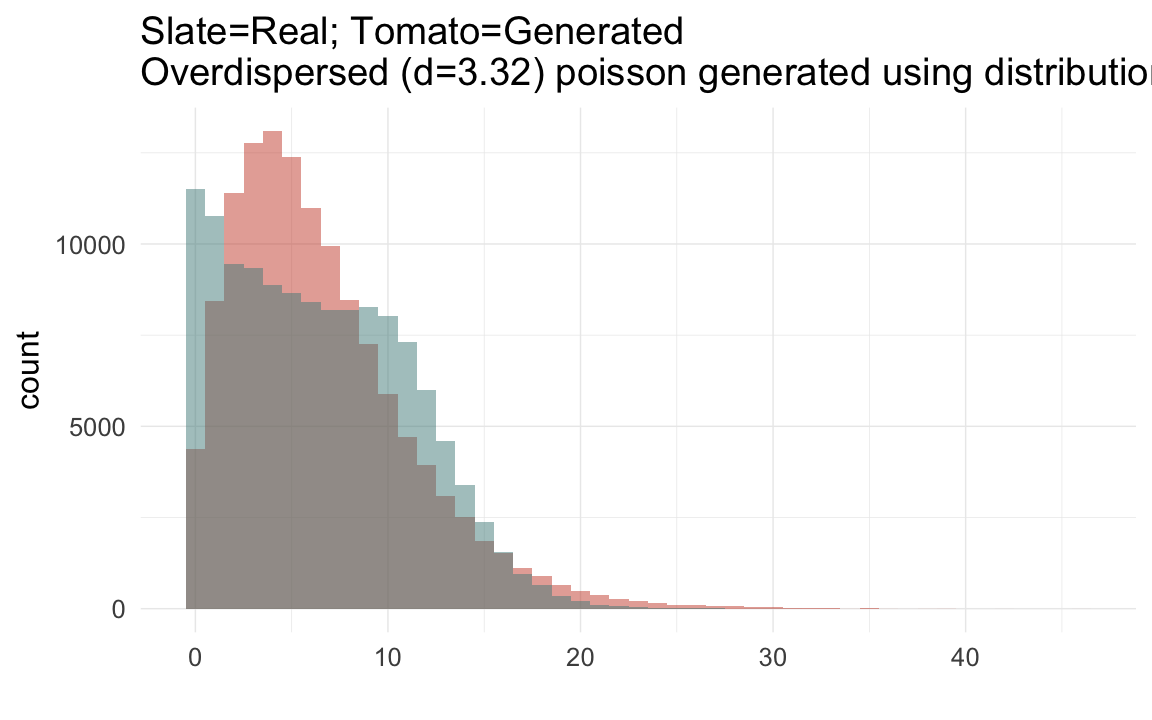
ggplot(data=rpqa, aes(x = paternalage.factor, y = survive1y)) +
    geom_pointrange(stat = "summary", fun.data = "mean_cl_boot", colour = "#aec05d") +
    desc_theme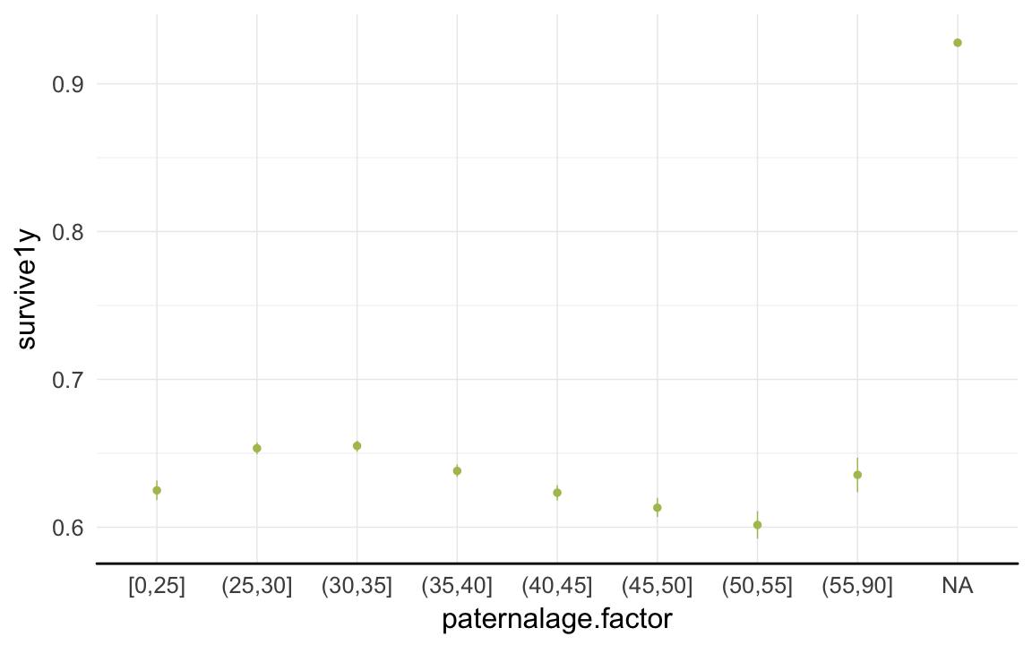
ggplot(data=rpqa[spouses > 0, ], aes(x = paternalage.factor, y = children)) +
    geom_pointrange(stat = "summary", fun.data = "mean_cl_boot", colour = "#aec05d") +
    desc_theme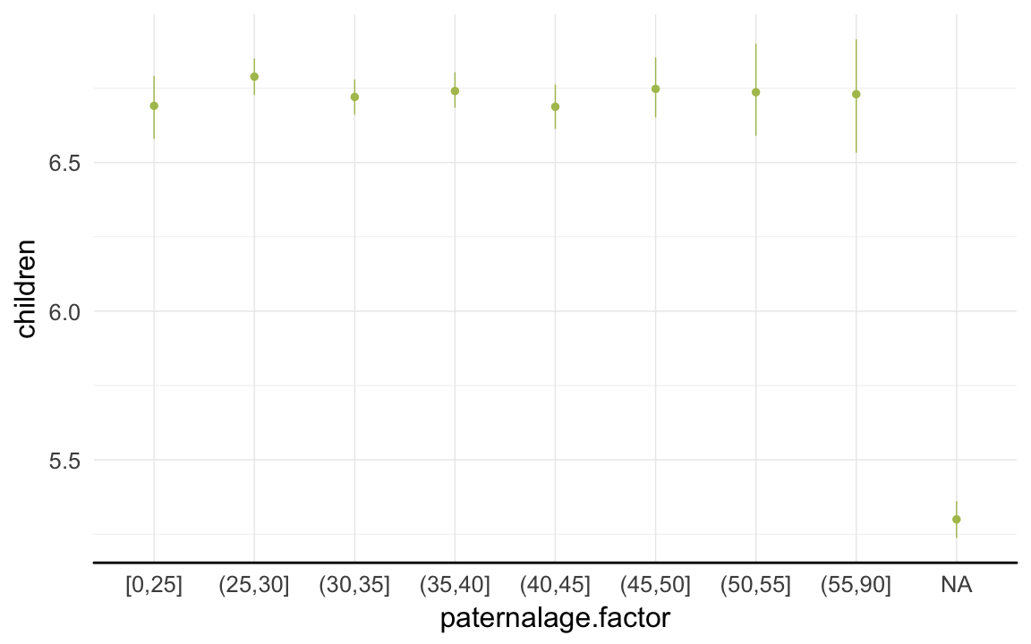
Opportunities for selection
rpqa.1$birth.decade = round(rpqa.1$byear/5)*5

episodes = rpqa.1 %>%
    filter(!is.na(male) | !is.na(survive1y) | !is.na(ever_married)) %>%
    group_by(birth.decade) %>%
    summarise(
        "Population size" = as.numeric(length(idIndividu)),
        "0. Number of children" = ifelse(between(birth.decade, 1670,1750), cva(children), NA_real_ ),
        "1. Surviving first year" = ifelse(between(birth.decade, 1670, 1755),cva_bin(survive1y), NA_real_ ),
        "2. Surviving to 15" = ifelse(between(birth.decade, 1670,1735), cva_bin(surviveR[survive1y==T]), NA_real_ ),
        "3. Ever married" = ifelse(between(birth.decade, 1670,1720), cva_bin(ever_married[surviveR==1]), NA_real_ ),
        "4. Number of children" = ifelse(between(birth.decade, 1670,1750), cva(children[ever_married==1]), NA_real_ ),
        "5. Grandchildren" = ifelse(between(birth.decade, 1670,1670), cva(grandchildren[children>0]), NA_real_ )
        ) %>%
#       mutate(male = Recode(male, "'NO'='female';''='male'")) %>%
    data.table()
data.frame(episodes[order(birth.decade), ], check.names = F)| birth.decade | Population size | 0. Number of children | 1. Surviving first year | 2. Surviving to 15 | 3. Ever married | 4. Number of children | 5. Grandchildren |
|---|---|---|---|---|---|---|---|
| 1670 | 1362 | 1.16 | 0.3481 | 0.206 | 0.4818 | 0.5963 | 0.7589 |
| 1675 | 2575 | 1.152 | 0.2827 | 0.2802 | 0.4755 | 0.5918 | NA |
| 1680 | 2598 | 1.194 | 0.3456 | 0.3456 | 0.492 | 0.5668 | NA |
| 1685 | 2621 | 1.225 | 0.4315 | 0.3557 | 0.4831 | 0.5743 | NA |
| 1690 | 3072 | 1.186 | 0.4459 | 0.3217 | 0.489 | 0.5675 | NA |
| 1695 | 3793 | 1.152 | 0.3861 | 0.3186 | 0.4767 | 0.5889 | NA |
| 1700 | 5025 | 1.232 | 0.4737 | 0.3785 | 0.477 | 0.5806 | NA |
| 1705 | 5181 | 1.184 | 0.4266 | 0.3267 | 0.4665 | 0.604 | NA |
| 1710 | 5771 | 1.219 | 0.4166 | 0.3762 | 0.4767 | 0.6196 | NA |
| 1715 | 6337 | 1.314 | 0.5281 | 0.3753 | 0.4776 | 0.6222 | NA |
| 1720 | 7184 | 1.246 | 0.447 | 0.3729 | 0.4605 | 0.6389 | NA |
| 1725 | 8520 | 1.373 | 0.4917 | 0.4278 | NA | 0.669 | NA |
| 1730 | 10200 | 1.55 | 0.5842 | 0.4982 | NA | 0.6784 | NA |
| 1735 | 11112 | 1.463 | 0.5627 | 0.3746 | NA | 0.696 | NA |
| 1740 | 4544 | 1.386 | 0.5384 | NA | NA | 0.6639 | NA |
save(episodes, file = "coefs/rpqa_episodes.rdata")
# rpqa.1 = merge(rpqa.1, episodes, by = "birth.decade", all.x = T)(episodes.plot = ggplot(melt(episodes,id.vars=c('birth.decade'), na.rm = T)) + geom_line(aes(x=birth.decade, y=value)) + facet_wrap(~ variable,scales='free_y',ncol = 1)) + mymin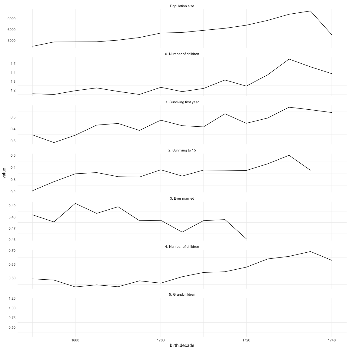
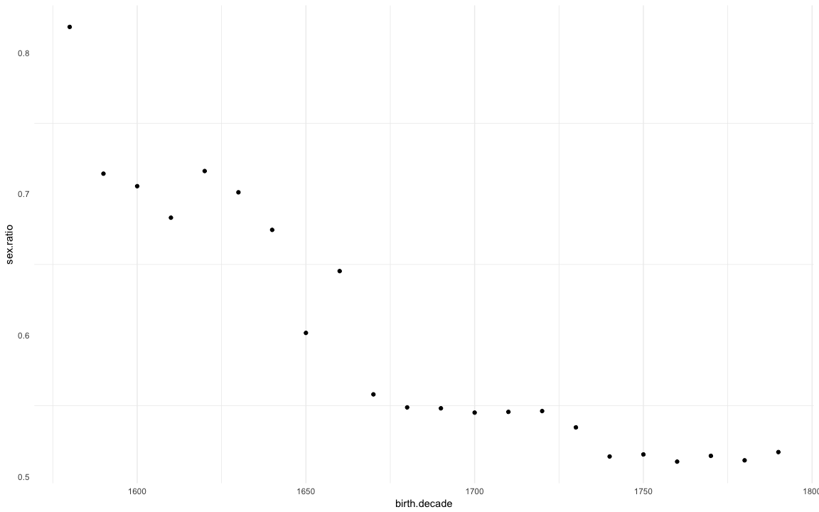
Sex ratio
rpqa$birth.decade = plyr::round_any(rpqa$byear, 10, floor)
(sex.ratio = rpqa %>%
    filter(!is.na(male)) %>%
    mutate(male = as.numeric(as.character(male))) %>%
    group_by(birth.decade) %>%
    summarise(sex.ratio = sum(male)/length(male)) %>%
    data.frame()
)| birth.decade | sex.ratio |
|---|---|
| 1640 | 0.6745 |
| 1710 | 0.5456 |
| NA | 0.5501 |
| 1690 | 0.5482 |
| 1700 | 0.5451 |
| 1670 | 0.558 |
| 1680 | 0.5488 |
| 1650 | 0.6016 |
| 1720 | 0.5462 |
| 1730 | 0.5347 |
| 1740 | 0.5141 |
| 1630 | 0.7011 |
| 1620 | 0.7162 |
| 1660 | 0.6453 |
| 1750 | 0.5155 |
| 1610 | 0.6831 |
| 1600 | 0.7054 |
| 1590 | 0.7143 |
| 1760 | 0.5104 |
| 1780 | 0.5113 |
| 1770 | 0.5145 |
| 1580 | 0.8182 |
| 1790 | 0.5172 |
ggplot(na.omit(sex.ratio)) + geom_point(aes(x=birth.decade, y=sex.ratio)) + mymin