Modern Sweden descriptives
Loading details
# bsub -q fat -W 48:00 -n 1 Rscript -e "setwd('/usr/users/rarslan/updated_data/'); filebase = '1_swed_descriptives'; knitr::knit(input = paste0(filebase,'.Rmd'), output = paste0(filebase,'.md'));cat(readLines(paste0(filebase,'.md')), sep = '\n')"

source("0__helpers.R")
opts_chunk$set(render = pander_handler, cache=F,cache.lazy=F,tidy=FALSE,autodep=TRUE,dev='png',fig.width=12,fig.height=7.5)
# load("swed.rdata")
load("swed.rdata")
load("swed1.rdata")
load("swed2.rdata")

demo_trends = aggDemoTrends(swed)
desc_theme = theme_minimal(base_size = 24)
update_geom_defaults("bar",   list(fill = "#6c92b2", alpha = 1/2))

mymin = theme_minimal() +theme(panel.grid.major.y =element_blank(),panel.grid.major.x = element_line(colour="#eeeeee"))

swed.1[, paternalage := 10 * paternalage]; swed[, paternalage := 10 * paternalage]; swed.2[, paternalage := 10 * paternalage];
swed.1[, maternalage := 10 * maternalage]; swed[, maternalage := 10 * maternalage]; swed.2[, maternalage := 10 * maternalage];
swed.1[, age_at_1st_child := 10 * age_at_1st_child]; swed[, age_at_1st_child := 10 * age_at_1st_child]; swed.2[, age_at_1st_child := 10 * age_at_1st_child]
swed.1[, age_at_last_child := 10 * age_at_last_child]; swed[, age_at_last_child := 10 * age_at_last_child]; swed.2[, age_at_last_child := 10 * age_at_last_child]
Variable descriptives
Whole population (N = 8201968)
descriptives = psych::describe(swed[, list(
    paternalage, maternalage, nr.siblings, dependent_sibs_f5y, age, spouses, children, grandchildren, byear, byear.Father, age_at_1st_child, age_at_last_child  )], check = F, fast = F)
round(data.frame(descriptives)[,2:12],2)| n | mean | sd | median | trimmed | mad | min | max | range | skew | kurtosis | |
|---|---|---|---|---|---|---|---|---|---|---|---|
| paternalage | 8190390 | 31.59 | 6.62 | 31 | 31.16 | 5.93 | 14 | 80 | 66 | 0.72 | 0.85 |
| maternalage | 8133674 | 28.39 | 5.67 | 28 | 28.17 | 5.93 | 13 | 60 | 47 | 0.34 | -0.34 |
| nr.siblings | 8201968 | 1.52 | 1.33 | 1 | 1.36 | 1.48 | 0 | 17 | 17 | 1.86 | 6.67 |
| dependent_sibs_f5y | 8201968 | 104.2 | 1374 | 1 | 0.9 | 1.48 | 0 | 25899 | 25899 | 15.08 | 239.5 |
| age | 352038 | 46.78 | 22.72 | 55 | 49.3 | 17.79 | 0 | 78 | 78 | -0.85 | -0.48 |
| spouses | 6417334 | 0.67 | 0.75 | 1 | 0.57 | 1.48 | 0 | 9 | 9 | 0.88 | 0.23 |
| children | 8201968 | 1.03 | 1.27 | 0 | 0.85 | 0 | 0 | 17 | 17 | 1.04 | 0.8 |
| grandchildren | 8201968 | 0.62 | 1.65 | 0 | 0.16 | 0 | 0 | 87 | 87 | 3.62 | 20.44 |
| byear | 8201968 | 1972 | 21.38 | 1972 | 1972 | 26.69 | 1932 | 2009 | 77 | -0.01 | -1.15 |
| byear.Father | 8190390 | 1940 | 22.29 | 1943 | 1941 | 26.69 | 1854 | 1995 | 141 | -0.2 | -0.91 |
| age_at_1st_child | 3878612 | 26.75 | 5.21 | 26 | 26.45 | 4.45 | 13 | 68 | 55 | 0.62 | 0.58 |
| age_at_last_child | 3878612 | 31.31 | 5.56 | 31 | 31.15 | 5.93 | 13 | 74 | 61 | 0.4 | 0.68 |
describeBin(swed[, list(survive1y, surviveR, ever_married)])| n | mean | sd | |
|---|---|---|---|
| survive1y | 5506833 | 0.97 | 0.03 |
| surviveR | 5503241 | 0.71 | 0.21 |
| ever_married | 6417334 | 0.51 | 0.25 |
pander(xtabs(~ paternal_loss, swed), caption = "Paternal loss at age")| later | [0,1] | (1,5] | (5,10] | (10,15] | (15,20] | (20,25] | (25,30] | (30,35] | (35,40] | (40,45] | unclear |
|---|---|---|---|---|---|---|---|---|---|---|---|
| 1096763 | 7248 | 19961 | 38395 | 63816 | 108260 | 170261 | 251155 | 328328 | 394178 | 339366 | 5384237 |
pander(xtabs(~ maternal_loss, swed), caption = "Maternal loss at age")| later | [0,1] | (1,5] | (5,10] | (10,15] | (15,20] | (20,25] | (25,30] | (30,35] | (35,40] | (40,45] | unclear |
|---|---|---|---|---|---|---|---|---|---|---|---|
| 1274984 | 2151 | 7869 | 16189 | 27191 | 45547 | 71480 | 106952 | 149433 | 204279 | 208744 | 6087149 |
included sample for reproductive outcomes (N = 1419282)
descriptives = psych::describe(swed.1[, list(
    paternalage, maternalage, nr.siblings, dependent_sibs_f5y, age, spouses, children, grandchildren, byear, byear.Father, age_at_1st_child, age_at_last_child  )], check = F, fast = F)
round(data.frame(descriptives)[,2:12],2)| n | mean | sd | median | trimmed | mad | min | max | range | skew | kurtosis | |
|---|---|---|---|---|---|---|---|---|---|---|---|
| paternalage | 1419282 | 31.84 | 7.05 | 31 | 31.4 | 7.41 | 14 | 79 | 65 | 0.65 | 0.43 |
| maternalage | 1408212 | 28.34 | 6.11 | 28 | 28.05 | 5.93 | 13 | 57 | 44 | 0.4 | -0.46 |
| nr.siblings | 1419282 | 1.81 | 1.55 | 1 | 1.62 | 1.48 | 0 | 16 | 16 | 1.63 | 4.63 |
| dependent_sibs_f5y | 1419282 | 68.24 | 799.3 | 1 | 0.93 | 1.48 | 0 | 12490 | 12490 | 12.3 | 154.7 |
| age | 79799 | 45.52 | 13.37 | 49 | 47.43 | 10.38 | 0 | 63 | 63 | -1.2 | 0.82 |
| spouses | 1403167 | 0.89 | 0.67 | 1 | 0.84 | 0 | 0 | 9 | 9 | 0.59 | 1.23 |
| children | 1419282 | 1.84 | 1.27 | 2 | 1.79 | 1.48 | 0 | 17 | 17 | 0.38 | 0.81 |
| grandchildren | 1419282 | 1.04 | 1.72 | 0 | 0.66 | 0 | 0 | 26 | 26 | 2.13 | 6.02 |
| byear | 1419282 | 1953 | 3.78 | 1953 | 1953 | 4.45 | 1947 | 1959 | 12 | 0.04 | -1.24 |
| byear.Father | 1419282 | 1921 | 8.19 | 1922 | 1921 | 7.41 | 1869 | 1945 | 76 | -0.43 | 0.16 |
| age_at_1st_child | 1133166 | 26.52 | 5.56 | 26 | 26.12 | 5.93 | 13 | 62 | 49 | 0.77 | 0.84 |
| age_at_last_child | 1133166 | 31.93 | 6 | 32 | 31.77 | 5.93 | 13 | 62 | 49 | 0.35 | 0.39 |
describeBin(swed.1[, list(ever_married)])| n | mean | sd | |
|---|---|---|---|
| ever_married | 1403167 | 0.74 | 0.19 |
pander(xtabs(~ paternal_loss, swed.1), caption = "Paternal loss at age")| later | [0,1] | (1,5] | (5,10] | (10,15] | (15,20] | (20,25] | (25,30] | (30,35] | (35,40] | (40,45] | unclear |
|---|---|---|---|---|---|---|---|---|---|---|---|
| 461355 | 169 | 1499 | 7282 | 20502 | 37218 | 57793 | 83348 | 110665 | 140572 | 132256 | 366623 |
pander(xtabs(~ maternal_loss, swed.1), caption = "Maternal loss at age")| later | [0,1] | (1,5] | (5,10] | (10,15] | (15,20] | (20,25] | (25,30] | (30,35] | (35,40] | (40,45] | unclear |
|---|---|---|---|---|---|---|---|---|---|---|---|
| 457633 | 127 | 685 | 3133 | 8714 | 14968 | 22170 | 32509 | 48389 | 72041 | 81128 | 677785 |
included sample for survival outcomes (N = 3428225)
descriptives = psych::describe(swed.2[, list(
    paternalage, maternalage, nr.siblings, dependent_sibs_f5y, age, byear, byear.Father, age_at_1st_child, age_at_last_child    )], check = F, fast = F)
round(data.frame(descriptives)[,2:12],2)| n | mean | sd | median | trimmed | mad | min | max | range | skew | kurtosis | |
|---|---|---|---|---|---|---|---|---|---|---|---|
| paternalage | 3428225 | 30.87 | 6.06 | 30 | 30.45 | 5.93 | 14 | 80 | 66 | 0.82 | 1.31 |
| maternalage | 3409118 | 27.95 | 5.17 | 28 | 27.76 | 5.93 | 13 | 59 | 46 | 0.35 | -0.15 |
| nr.siblings | 3428225 | 1.46 | 1.15 | 1 | 1.34 | 1.48 | 0 | 17 | 17 | 1.88 | 8.18 |
| dependent_sibs_f5y | 3428225 | 24.73 | 364 | 1 | 0.94 | 0 | 0 | 6646 | 6646 | 15.63 | 247.1 |
| age | 43025 | 11.4 | 12.42 | 5 | 9.95 | 7.41 | 0 | 41 | 41 | 0.61 | -1.06 |
| byear | 3428225 | 1984 | 8.9 | 1984 | 1984 | 11.86 | 1969 | 1999 | 30 | -0.06 | -1.22 |
| byear.Father | 3428225 | 1953 | 9.84 | 1953 | 1953 | 10.38 | 1890 | 1985 | 95 | -0.19 | -0.18 |
| age_at_1st_child | 907084 | 27.33 | 4.56 | 27 | 27.31 | 4.45 | 13 | 40 | 27 | 0.02 | -0.53 |
| age_at_last_child | 907084 | 30.05 | 4.48 | 30 | 30.19 | 4.45 | 14 | 40 | 26 | -0.29 | -0.33 |
describeBin(swed.2[, list(survive1y, surviveR, ever_married)])| n | mean | sd | |
|---|---|---|---|
| survive1y | 3428225 | 0.99 | 0.01 |
| surviveR | 3428214 | 0.81 | 0.15 |
| ever_married | 2744282 | 0.21 | 0.17 |
pander(xtabs(~ paternal_loss, swed.2), caption = "Paternal loss at age")| later | [0,1] | (1,5] | (5,10] | (10,15] | (15,20] | (20,25] | (25,30] | (30,35] | (35,40] | (40,45] | unclear |
|---|---|---|---|---|---|---|---|---|---|---|---|
| 0 | 4210 | 11510 | 20127 | 27532 | 34940 | 39891 | 42846 | 40920 | 25991 | 1509 | 3178749 |
pander(xtabs(~ maternal_loss, swed.2), caption = "Maternal loss at age")| later | [0,1] | (1,5] | (5,10] | (10,15] | (15,20] | (20,25] | (25,30] | (30,35] | (35,40] | (40,45] | unclear |
|---|---|---|---|---|---|---|---|---|---|---|---|
| 0 | 1177 | 4473 | 8547 | 12280 | 16071 | 19174 | 20695 | 20517 | 13909 | 955 | 3310427 |
Number of families with varying numbers of siblings available for comparison
crosstabs(swed[!duplicated(idParents), ]$nr.siblings)| 0 | 1 | 2 | 3 | 4 | 5 | 6 | 7 | 8 | 9 | 10 | 11 | 12 | 13 | 14 | 15 | 16 | 17 |
|---|---|---|---|---|---|---|---|---|---|---|---|---|---|---|---|---|---|
| 1438193 | 1679574 | 670639 | 191779 | 59147 | 22172 | 9399 | 4212 | 1949 | 928 | 426 | 218 | 98 | 37 | 15 | 9 | 6 | 1 |
qplot(swed.1[!duplicated(idParents), ]$nr.siblings, binwidth = 1) + xlab("Number of siblings per family") + desc_theme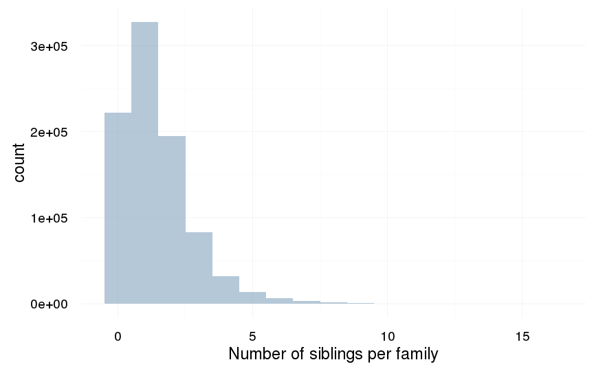
Missingness patterns
The first table shows the number of missings per variable, the second table, using the indexes from the first, shows missings in which variables tend to occur together. Most variables of interest in this study are derived from these dates and so these patterns can show many cases did not have the data to calculate e.g. paternal loss (those lacking either the father’s death date, the anchor’s birth date or both).
pander_escape(missingness_patterns(swed[, list(
    byear, dyear, byear.Father, dyear.Father, byear.Mother, dyear.Mother, education
    )]))
## index col missings
## 1 dyear 7849926
## 2 dyear.Mother 6084972
## 3 dyear.Father 5380461
## 4 education 2111673
## 5 byear.Mother 68294
## 6 byear.Father 11578| Pattern | Freq | Culprit |
|---|---|---|
| 1_2_3______ | 2959092 | |
| 1_2_3_4____ | 1935537 | |
| 1__________ | 1504260 | dyear |
| 1_2________ | 966229 | |
| 1___3______ | 347415 | |
| ___________ | 172918 | _ |
| __2_3_4____ | 40504 | |
| __2________ | 37058 | dyear.Mother |
| 1_2___4____ | 32376 | |
| 1_____4____ | 26614 | |
| 1_2_____5__ | 26592 | |
| __2_3______ | 26072 | |
| ____3______ | 21513 | dyear.Father |
| ______4____ | 19844 | education |
| __2___4____ | 14825 | |
| 1_2_3___5__ | 12523 | |
| 1___3_4____ | 12427 | |
| 1_2_3_4_5__ | 11054 | |
| __2___4_5__ | 5946 | |
| ____3_4____ | 5926 | |
| __2_____5__ | 5228 | |
| 1_2_______6 | 3018 | |
| 1_2_3_4___6 | 1984 | |
| 1_2_3_____6 | 1982 | |
| 1_________6 | 1819 | |
| 1___3___5__ | 1603 | |
| 1_2___4___6 | 1446 | |
| 1_2___4_5__ | 1389 | |
| 1_______5__ | 1096 | |
| __2_3___5__ | 785 | |
| __2_3_4_5__ | 715 | |
| 1___3_4_5__ | 599 | |
| 1___3_____6 | 290 | |
| __________6 | 282 | byear.Father |
| 1_2_3_4_5_6 | 175 | |
| ________5__ | 150 | byear.Mother |
| 1_2_3___5_6 | 123 | |
| 1_2_____5_6 | 94 | |
| 1_2___4_5_6 | 64 | |
| __2_______6 | 48 | |
| 1_____4_5__ | 39 | |
| 1_____4___6 | 38 | |
| __2_3_4___6 | 37 | |
| __2___4___6 | 36 | |
| ______4___6 | 27 | |
| ______4_5__ | 24 | |
| ____3___5__ | 23 | |
| 1_______5_6 | 22 | |
| ____3_____6 | 21 | |
| __2_3_____6 | 19 | |
| 1___3_4___6 | 14 | |
| ____3_4_5__ | 14 | |
| __2_____5_6 | 12 | |
| 1_____4_5_6 | 7 | |
| __2_3_4_5_6 | 4 | |
| 1___3___5_6 | 3 | |
| __2___4_5_6 | 3 | |
| ____3_4___6 | 3 | |
| ________5_6 | 3 | |
| 1___3_4_5_6 | 2 | |
| __2_3___5_6 | 2 |
Reproductive timing
ggplot(data = demo_trends) +
    geom_line(aes(x= Year, y = first, linetype = "first", colour = Parent),  size = 1) +
  geom_line(aes(x = Year, y = all, linetype = "all", colour = Parent), size = 1) +
    geom_line(aes(x= Year, y = last, linetype = "last", colour = Parent),size = 1) +
    scale_colour_manual(values = c(Father = "#6c92b2", Mother = "#aec05d")) +
    scale_linetype_manual("Birth", breaks = c("last", "all","first"), values = c( "solid","dashed", "dotted")) +
    scale_y_continuous("Parental age at birth", limits = c(23,40)) +
        geom_text(aes(x = Year, y = all + 0.31,
                                    label = ifelse(Year %% 15 == 0, round(all), NA))) +
    facet_wrap(~ Parent) +
    desc_theme + theme(legend.position = c(1,1),
  legend.justification = c(1,1),
  legend.box = "horizontal",
  panel.margin = unit(2, "lines"))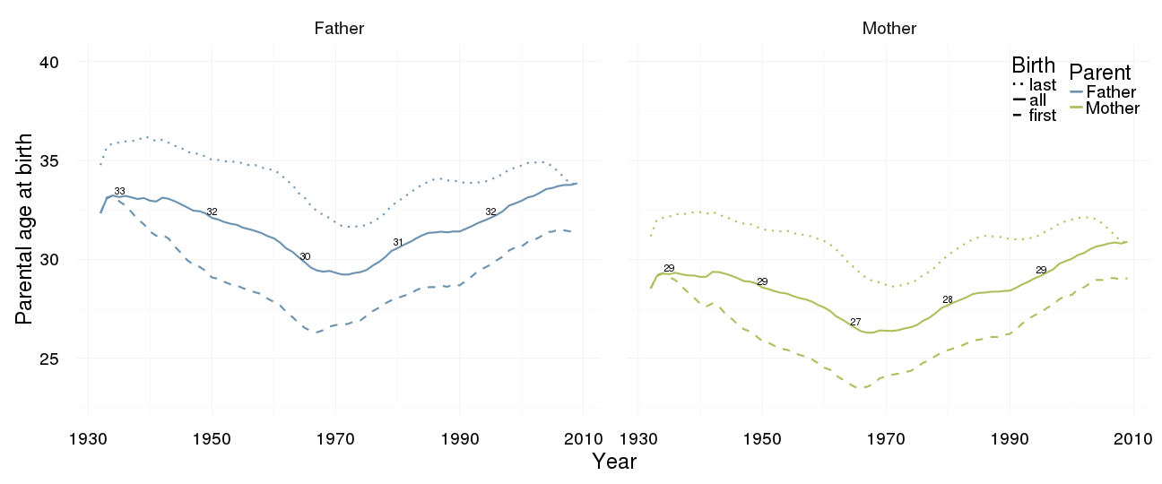
Correlations between variables
round(cor(swed.1[, list(
    paternalage, maternalage, birthorder, nr.siblings, children, grandchildren, byear, byear.Father, age_at_1st_child, age_at_last_child
)], use = "pairwise.complete.obs"),2)| paternalage | maternalage | birthorder | nr.siblings | children | grandchildren | byear | byear.Father | age_at_1st_child | age_at_last_child | |
|---|---|---|---|---|---|---|---|---|---|---|
| paternalage | 1 | 0.77 | 0.43 | 0.13 | -0.03 | -0.03 | -0.06 | -0.89 | 0.06 | 0.03 |
| maternalage | 0.77 | 1 | 0.45 | 0.09 | -0.04 | -0.04 | -0.06 | -0.69 | 0.08 | 0.04 |
| birthorder | 0.43 | 0.45 | 1 | 0.7 | 0.04 | 0.05 | 0 | -0.37 | -0.06 | -0.03 |
| nr.siblings | 0.13 | 0.09 | 0.7 | 1 | 0.08 | 0.09 | -0.01 | -0.11 | -0.09 | -0.03 |
| children | -0.03 | -0.04 | 0.04 | 0.08 | 1 | 0.43 | -0.01 | 0.02 | -0.28 | 0.38 |
| grandchildren | -0.03 | -0.04 | 0.05 | 0.09 | 0.43 | 1 | -0.33 | -0.12 | -0.53 | -0.25 |
| byear | -0.06 | -0.06 | 0 | -0.01 | -0.01 | -0.33 | 1 | 0.51 | 0.13 | 0.09 |
| byear.Father | -0.89 | -0.69 | -0.37 | -0.11 | 0.02 | -0.12 | 0.51 | 1 | 0.01 | 0.01 |
| age_at_1st_child | 0.06 | 0.08 | -0.06 | -0.09 | -0.28 | -0.53 | 0.13 | 0.01 | 1 | 0.62 |
| age_at_last_child | 0.03 | 0.04 | -0.03 | -0.03 | 0.38 | -0.25 | 0.09 | 0.01 | 0.62 | 1 |
ggplot(data=swed, aes(x = byear, y = paternalage)) +
    geom_linerange(stat = "summary", fun.data = "mean_sdl", colour = "#aec05d") +
    geom_pointrange(stat = "summary", fun.data = "mean_cl_boot", colour = "#6c92b2") +
    desc_theme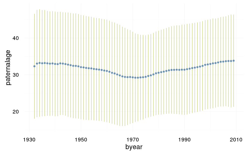
ggplot(data=swed, aes(x = byear, y = age_at_1st_child)) +
    geom_linerange(stat = "summary", fun.data = "median_hilow", colour = "#aec05d") +
    geom_pointrange(stat = "summary", fun.data = "mean_cl_boot", colour = "#6c92b2") +
    desc_theme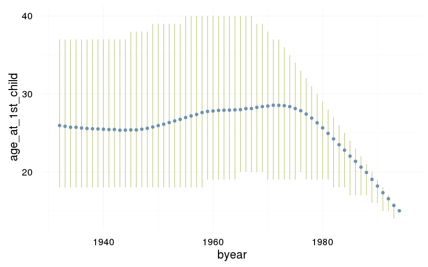
ggplot(data=swed, aes(x = byear, y = age_at_last_child)) +
    geom_linerange(stat = "summary", fun.data = "median_hilow", colour = "#aec05d") +
    geom_pointrange(stat = "summary", fun.data = "mean_cl_boot", colour = "#6c92b2") +
    desc_theme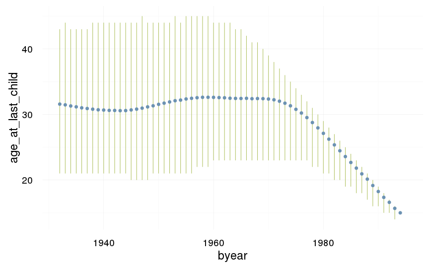
ggplot(data=swed, aes(x = byear, y = children)) +
    geom_linerange(stat = "summary", fun.data = "median_hilow", colour = "#aec05d") +
    geom_pointrange(stat = "summary", fun.data = "mean_cl_boot", colour = "#6c92b2") +

    desc_theme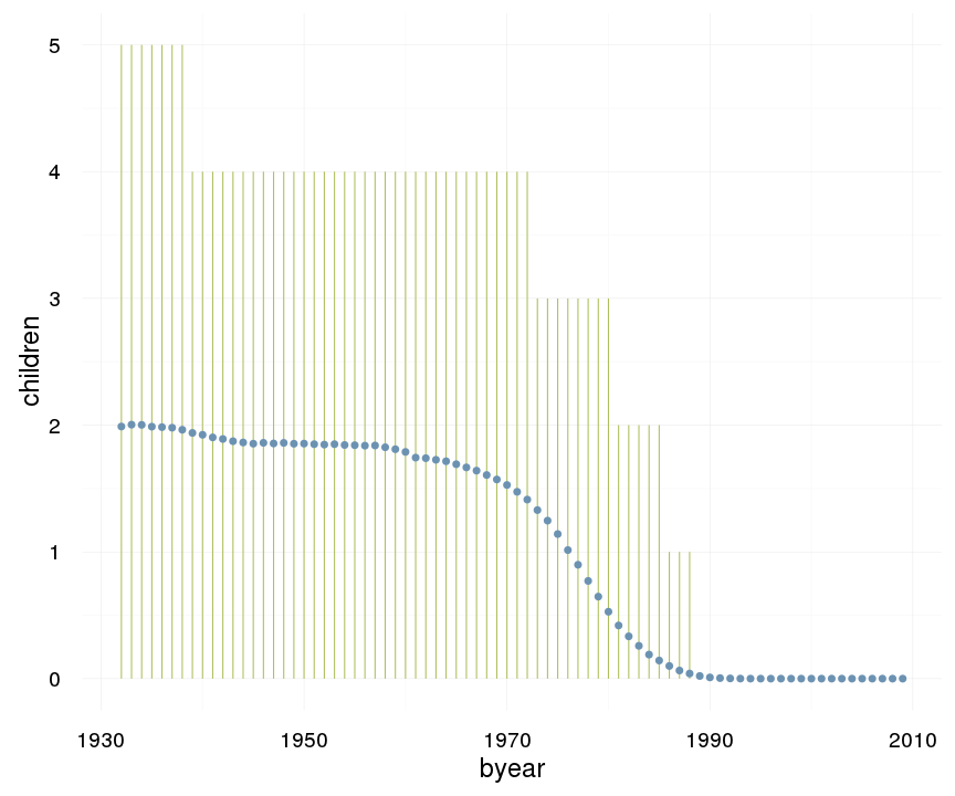
ggplot(data=swed, aes(x = byear, y = survive1y)) +
    geom_pointrange(stat = "summary", fun.data = "mean_cl_boot", colour = "#aec05d") +
    desc_theme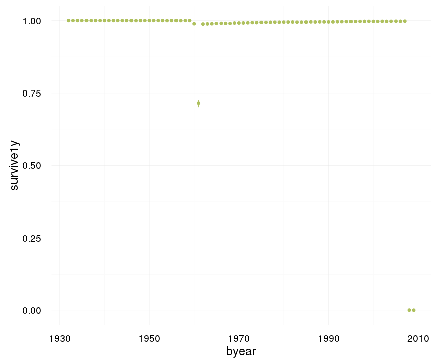
ggplot(data=swed, aes(x = byear, y = surviveR)) +
    geom_pointrange(stat = "summary", fun.data = "mean_cl_boot", colour = "#aec05d") +
    desc_theme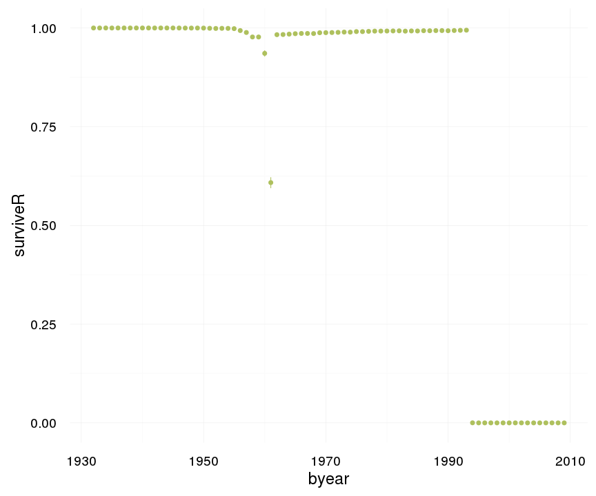
ggplot(data=swed.1, aes(x = children, y = grandchildren)) +
    geom_jitter(colour = "#aec05d", alpha = I(0.1)) +
    geom_pointrange(stat = "summary", fun.data = "median_hilow", colour = "#6c92b2") +
    geom_smooth(method = "glm", formula = y ~ poly(x,3), colour = "#6e85b0") +
    desc_theme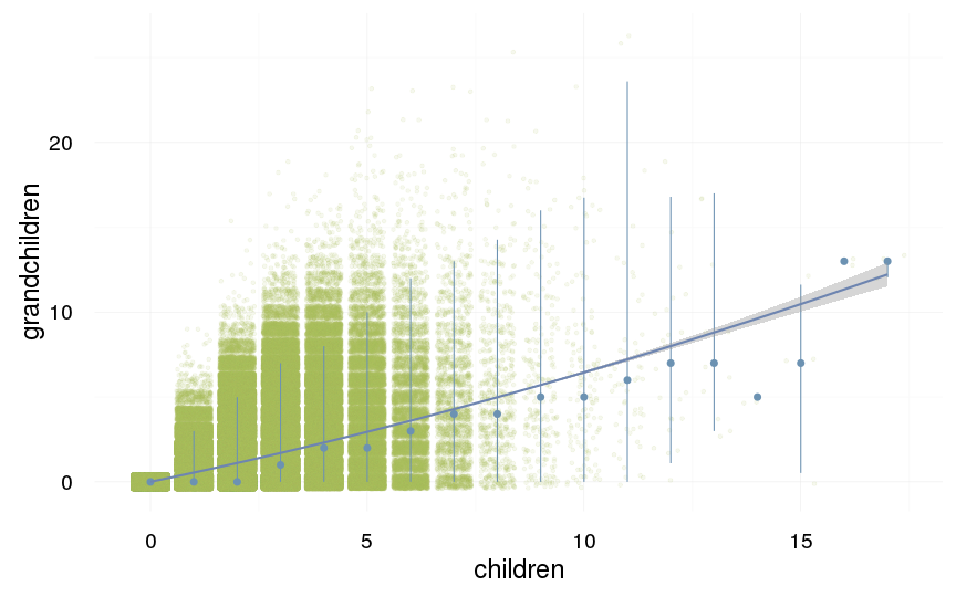
crosstabs(~ children + children.surviving5y, data = swed.1)| 0 | 1 | 2 | 3 | 4 | 5 | 6 | 7 | 8 | 9 | 10 | 11 | 12 | 13 | 14 | 15 | 16 | 17 | |
|---|---|---|---|---|---|---|---|---|---|---|---|---|---|---|---|---|---|---|
| 0 | 286116 | 0 | 0 | 0 | 0 | 0 | 0 | 0 | 0 | 0 | 0 | 0 | 0 | 0 | 0 | 0 | 0 | 0 |
| 1 | 2232 | 196720 | 0 | 0 | 0 | 0 | 0 | 0 | 0 | 0 | 0 | 0 | 0 | 0 | 0 | 0 | 0 | 0 |
| 2 | 553 | 3942 | 534577 | 0 | 0 | 0 | 0 | 0 | 0 | 0 | 0 | 0 | 0 | 0 | 0 | 0 | 0 | 0 |
| 3 | 33 | 439 | 8528 | 275295 | 0 | 0 | 0 | 0 | 0 | 0 | 0 | 0 | 0 | 0 | 0 | 0 | 0 | 0 |
| 4 | 4 | 39 | 580 | 5655 | 74696 | 0 | 0 | 0 | 0 | 0 | 0 | 0 | 0 | 0 | 0 | 0 | 0 | 0 |
| 5 | 0 | 0 | 33 | 374 | 2116 | 18419 | 0 | 0 | 0 | 0 | 0 | 0 | 0 | 0 | 0 | 0 | 0 | 0 |
| 6 | 0 | 0 | 1 | 29 | 157 | 677 | 5049 | 0 | 0 | 0 | 0 | 0 | 0 | 0 | 0 | 0 | 0 | 0 |
| 7 | 0 | 0 | 0 | 3 | 14 | 78 | 270 | 1508 | 0 | 0 | 0 | 0 | 0 | 0 | 0 | 0 | 0 | 0 |
| 8 | 0 | 0 | 0 | 0 | 4 | 5 | 31 | 108 | 522 | 0 | 0 | 0 | 0 | 0 | 0 | 0 | 0 | 0 |
| 9 | 0 | 0 | 0 | 1 | 0 | 0 | 3 | 11 | 39 | 192 | 0 | 0 | 0 | 0 | 0 | 0 | 0 | 0 |
| 10 | 0 | 0 | 0 | 0 | 0 | 0 | 0 | 1 | 8 | 23 | 99 | 0 | 0 | 0 | 0 | 0 | 0 | 0 |
| 11 | 0 | 0 | 0 | 0 | 0 | 0 | 0 | 0 | 1 | 5 | 5 | 42 | 0 | 0 | 0 | 0 | 0 | 0 |
| 12 | 0 | 0 | 0 | 0 | 0 | 0 | 0 | 0 | 0 | 1 | 1 | 3 | 18 | 0 | 0 | 0 | 0 | 0 |
| 13 | 0 | 0 | 0 | 0 | 0 | 0 | 0 | 0 | 0 | 1 | 0 | 1 | 4 | 5 | 0 | 0 | 0 | 0 |
| 14 | 0 | 0 | 0 | 0 | 0 | 0 | 0 | 0 | 0 | 0 | 0 | 0 | 0 | 0 | 2 | 0 | 0 | 0 |
| 15 | 0 | 0 | 0 | 0 | 0 | 0 | 0 | 0 | 0 | 0 | 0 | 0 | 0 | 1 | 0 | 3 | 0 | 0 |
| 16 | 0 | 0 | 0 | 0 | 0 | 0 | 0 | 0 | 0 | 0 | 0 | 0 | 0 | 0 | 0 | 0 | 2 | 0 |
| 17 | 0 | 0 | 0 | 0 | 0 | 0 | 0 | 0 | 0 | 0 | 0 | 0 | 0 | 0 | 0 | 0 | 1 | 2 |
ggplot(data=swed.1, aes(x = children, y = children.surviving5y)) +
    geom_jitter(colour = "#aec05d", alpha = I(0.1)) +
    geom_pointrange(stat = "summary", fun.data = "median_hilow", colour = "#6c92b2") +
    geom_smooth(method = "glm", formula = y ~ poly(x,3), colour = "#6e85b0") +
    desc_theme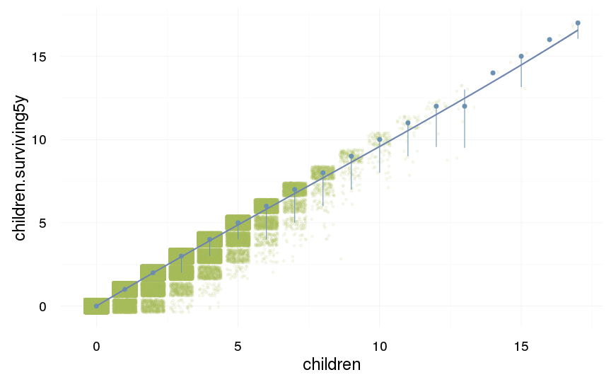
ggplot(data=swed.1, aes(x = round(age), y = children)) +
    geom_jitter(colour = "#aec05d", alpha = I(0.1)) +
    geom_pointrange(stat = "summary", fun.data = "mean_cl_boot", colour = "#6c92b2") +
    geom_smooth(colour = "#6e85b0") +
    xlab("Age") +
    ylab("Number of children") +
    desc_theme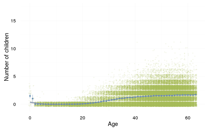
ggplot(data=swed.1[children>0,], aes(x = round(age), y = children)) +
    geom_jitter(colour = "#aec05d", alpha = I(0.1)) +
    geom_pointrange(stat = "summary", fun.data = "mean_cl_boot", colour = "#6c92b2") +
    geom_smooth(colour = "#6e85b0") +
    xlab("Age") +
    ylab("Number of children") +
    desc_theme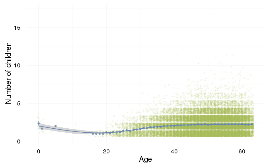
plot_zero_infl(swed.1[ spouses > 0, ]$children)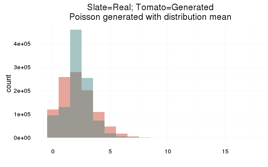
ggplot(data=swed.2, aes(x = paternalage.factor, y = survive1y)) +
    geom_pointrange(stat = "summary", fun.data = "mean_cl_boot", colour = "#aec05d") +
    desc_theme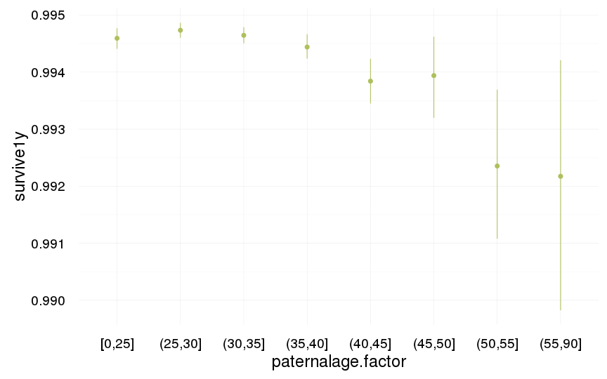
ggplot(data=swed.1[spouses > 0, ], aes(x = paternalage.factor, y = children)) +
    geom_pointrange(stat = "summary", fun.data = "mean_cl_boot", colour = "#aec05d") +
    desc_theme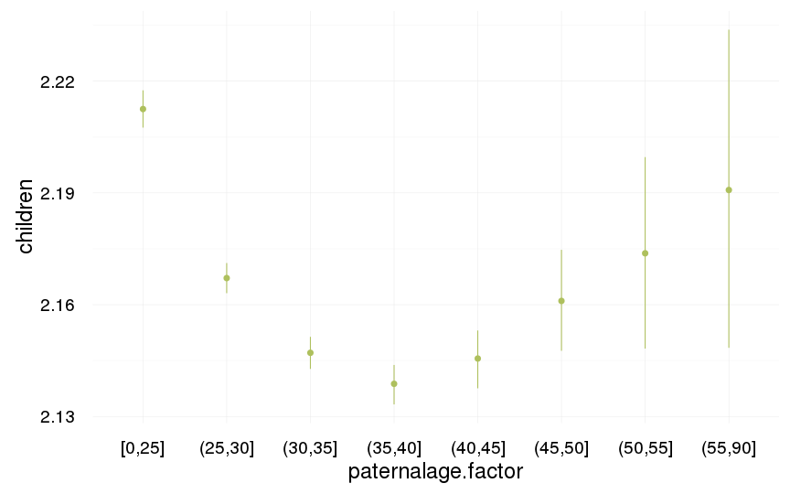
Opportunities for selection
swed$any_children = ifelse(swed$children > 0, 1, 0)
episodes = swed %>%
    filter(!is.na(male) | !is.na(survive1y) | !is.na(ever_married)) %>%
    group_by(byear) %>%
    summarise(
        "Population size" = as.numeric(length(idIndividu)),
        "0. Children " = ifelse(between(byear, 1947,1958), cva(children), NA_real_ ),
        "0. Any children" = ifelse(between(byear, 1947,1958), cva_bin(any_children), NA_real_ ),
        "1. Surviving first year" =  ifelse(between(byear, 1962,1990),cva_bin(survive1y), NA_real_ ),
        "2. Surviving to 15" = ifelse(between(byear, 1962,1977), cva_bin(surviveR[survive1y==T]), NA_real_ ),
        "3. Ever married" = ifelse(between(byear, 1947,1960), cva_bin(ever_married[surviveR==1]), NA_real_ ),
        "4. Children" = ifelse(between(byear, 1947,1958), cva(children[ever_married==1]), NA_real_ ),
        "5. Grandchildren" = ifelse(between(byear, 1947,1947), cva(grandchildren[children>0]), NA_real_ )
        ) %>%
    setDT()

data.frame(episodes[order(byear), ])| byear | Population.size | X0..Children. | X0..Any.children | X1..Surviving.first.year | X2..Surviving.to.15 | X3..Ever.married | X4..Children | X5..Grandchildren |
|---|---|---|---|---|---|---|---|---|
| 1932 | 27052 | NA | NA | NA | NA | NA | NA | NA |
| 1933 | 49286 | NA | NA | NA | NA | NA | NA | NA |
| 1934 | 59173 | NA | NA | NA | NA | NA | NA | NA |
| 1935 | 63903 | NA | NA | NA | NA | NA | NA | NA |
| 1936 | 68781 | NA | NA | NA | NA | NA | NA | NA |
| 1937 | 71236 | NA | NA | NA | NA | NA | NA | NA |
| 1938 | 75451 | NA | NA | NA | NA | NA | NA | NA |
| 1939 | 79599 | NA | NA | NA | NA | NA | NA | NA |
| 1940 | 79772 | NA | NA | NA | NA | NA | NA | NA |
| 1941 | 85605 | NA | NA | NA | NA | NA | NA | NA |
| 1942 | 1e+05 | NA | NA | NA | NA | NA | NA | NA |
| 1943 | 110883 | NA | NA | NA | NA | NA | NA | NA |
| 1944 | 119153 | NA | NA | NA | NA | NA | NA | NA |
| 1945 | 120772 | NA | NA | NA | NA | NA | NA | NA |
| 1946 | 121667 | NA | NA | NA | NA | NA | NA | NA |
| 1947 | 119906 | 0.6579 | 0.4644 | NA | NA | 0.6918 | 0.5278 | 0.9062 |
| 1948 | 118922 | 0.6627 | 0.4688 | NA | NA | 0.725 | 0.5268 | NA |
| 1949 | 114845 | 0.6716 | 0.4771 | NA | NA | 0.7657 | 0.5304 | NA |
| 1950 | 110148 | 0.6752 | 0.4838 | NA | NA | 0.8218 | 0.5286 | NA |
| 1951 | 105577 | 0.6889 | 0.4947 | NA | NA | 0.895 | 0.5336 | NA |
| 1952 | 106774 | 0.6898 | 0.5005 | NA | NA | 0.9525 | 0.5279 | NA |
| 1953 | 107538 | 0.6951 | 0.505 | NA | NA | 1.001 | 0.5331 | NA |
| 1954 | 103736 | 0.6987 | 0.5119 | NA | NA | 1.061 | 0.5286 | NA |
| 1955 | 106383 | 0.7038 | 0.5179 | NA | NA | 1.141 | 0.5314 | NA |
| 1956 | 107608 | 0.7085 | 0.5244 | NA | NA | 1.172 | 0.5326 | NA |
| 1957 | 107128 | 0.7086 | 0.5274 | NA | NA | 1.239 | 0.5285 | NA |
| 1958 | 105759 | 0.7099 | 0.5305 | NA | NA | 1.286 | 0.5296 | NA |
| 1959 | 106062 | NA | NA | NA | NA | 1.334 | NA | NA |
| 1960 | 103898 | NA | NA | NA | NA | 1.44 | NA | NA |
| 1961 | 108905 | NA | NA | NA | NA | NA | NA | NA |
| 1962 | 111569 | NA | NA | 0.1116 | 0.06899 | NA | NA | NA |
| 1963 | 117652 | NA | NA | 0.1091 | 0.06994 | NA | NA | NA |
| 1964 | 127455 | NA | NA | 0.1066 | 0.06633 | NA | NA | NA |
| 1965 | 127698 | NA | NA | 0.1023 | 0.06465 | NA | NA | NA |
| 1966 | 127726 | NA | NA | 0.0999 | 0.06332 | NA | NA | NA |
| 1967 | 126358 | NA | NA | 0.1007 | 0.06174 | NA | NA | NA |
| 1968 | 118625 | NA | NA | 0.1019 | 0.06217 | NA | NA | NA |
| 1969 | 112567 | NA | NA | 0.09371 | 0.05815 | NA | NA | NA |
| 1970 | 114364 | NA | NA | 0.09316 | 0.05753 | NA | NA | NA |
| 1971 | 118423 | NA | NA | 0.09247 | 0.05584 | NA | NA | NA |
| 1972 | 117025 | NA | NA | 0.08945 | 0.05647 | NA | NA | NA |
| 1973 | 114983 | NA | NA | 0.08506 | 0.05702 | NA | NA | NA |
| 1974 | 115800 | NA | NA | 0.0863 | 0.05629 | NA | NA | NA |
| 1975 | 109598 | NA | NA | 0.08018 | 0.0523 | NA | NA | NA |
| 1976 | 104096 | NA | NA | 0.08024 | 0.05303 | NA | NA | NA |
| 1977 | 102021 | NA | NA | 0.07756 | 0.0507 | NA | NA | NA |
| 1978 | 99404 | NA | NA | 0.07648 | NA | NA | NA | NA |
| 1979 | 102788 | NA | NA | 0.07624 | NA | NA | NA | NA |
| 1980 | 104171 | NA | NA | 0.07411 | NA | NA | NA | NA |
| 1981 | 101478 | NA | NA | 0.07301 | NA | NA | NA | NA |
| 1982 | 101023 | NA | NA | 0.07214 | NA | NA | NA | NA |
| 1983 | 100255 | NA | NA | 0.07595 | NA | NA | NA | NA |
| 1984 | 102913 | NA | NA | 0.0745 | NA | NA | NA | NA |
| 1985 | 107518 | NA | NA | 0.07345 | NA | NA | NA | NA |
| 1986 | 110995 | NA | NA | 0.06894 | NA | NA | NA | NA |
| 1987 | 113599 | NA | NA | 0.07114 | NA | NA | NA | NA |
| 1988 | 121462 | NA | NA | 0.06836 | NA | NA | NA | NA |
| 1989 | 125042 | NA | NA | 0.06856 | NA | NA | NA | NA |
| 1990 | 132883 | NA | NA | 0.07006 | NA | NA | NA | NA |
| 1991 | 131987 | NA | NA | NA | NA | NA | NA | NA |
| 1992 | 129699 | NA | NA | NA | NA | NA | NA | NA |
| 1993 | 123604 | NA | NA | NA | NA | NA | NA | NA |
| 1994 | 118708 | NA | NA | NA | NA | NA | NA | NA |
| 1995 | 109684 | NA | NA | NA | NA | NA | NA | NA |
| 1996 | 101571 | NA | NA | NA | NA | NA | NA | NA |
| 1997 | 96803 | NA | NA | NA | NA | NA | NA | NA |
| 1998 | 95550 | NA | NA | NA | NA | NA | NA | NA |
| 1999 | 94648 | NA | NA | NA | NA | NA | NA | NA |
| 2000 | 96816 | NA | NA | NA | NA | NA | NA | NA |
| 2001 | 96994 | NA | NA | NA | NA | NA | NA | NA |
| 2002 | 101182 | NA | NA | NA | NA | NA | NA | NA |
| 2003 | 103929 | NA | NA | NA | NA | NA | NA | NA |
| 2004 | 105677 | NA | NA | NA | NA | NA | NA | NA |
| 2005 | 105620 | NA | NA | NA | NA | NA | NA | NA |
| 2006 | 109343 | NA | NA | NA | NA | NA | NA | NA |
| 2007 | 109601 | NA | NA | NA | NA | NA | NA | NA |
| 2008 | 109549 | NA | NA | NA | NA | NA | NA | NA |
| 2009 | 105981 | NA | NA | NA | NA | NA | NA | NA |
save(episodes, file = "coefs/swed_episodes.rdata")(episodes.plot = ggplot(melt(episodes,id.vars=c('byear'), na.rm = T)) + geom_line(aes(x=byear, y=value)) + facet_wrap(~ variable,scales='free_y',ncol = 1)) + mymin## geom_path: Each group consists of only one observation. Do you need to
## adjust the group aesthetic?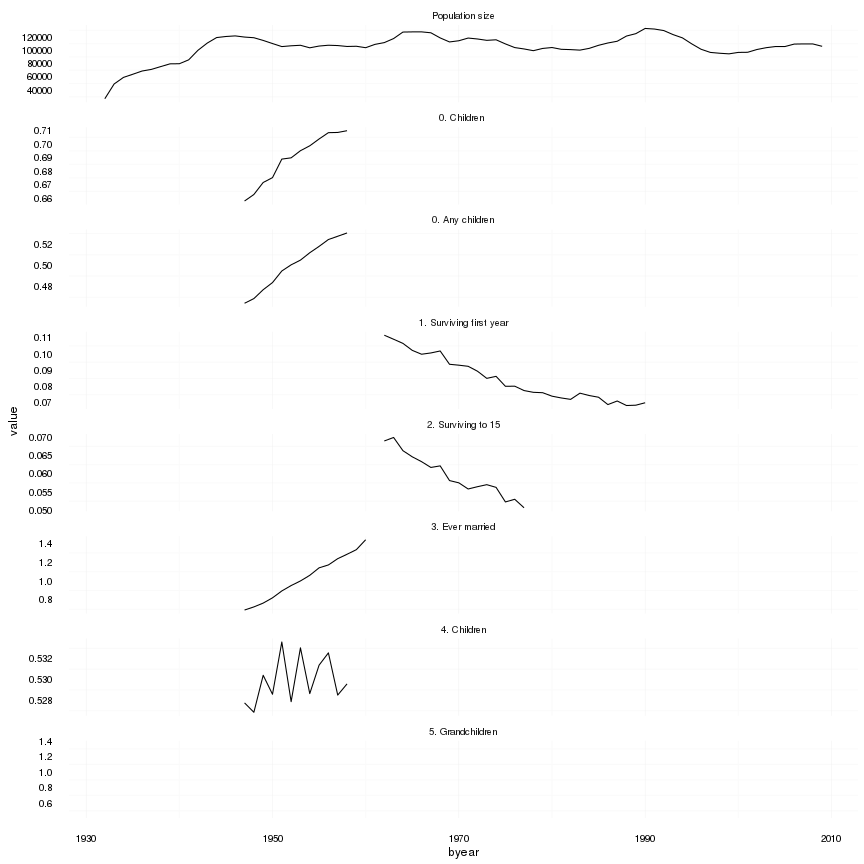
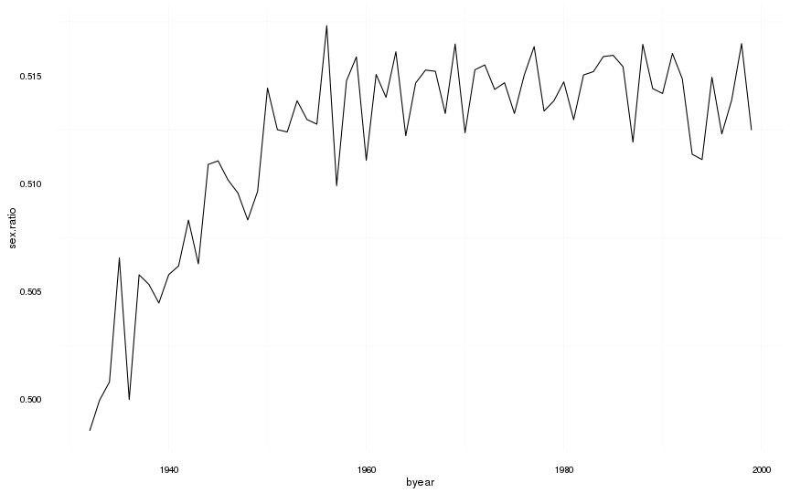
Sex ratio
(sex.ratio = swed %>%
    filter(!is.na(male) & byear < 2000) %>%
    mutate(male = as.numeric(as.character(male))) %>%
    group_by(byear) %>%
    summarise(sex.ratio = sum(male)/length(male)) %>%
    data.frame()
)| byear | sex.ratio |
|---|---|
| 1952 | 0.5124 |
| 1983 | 0.5152 |
| 1934 | 0.5008 |
| 1999 | 0.5125 |
| 1943 | 0.5063 |
| 1972 | 0.5155 |
| 1940 | 0.5058 |
| 1977 | 0.5164 |
| 1996 | 0.5123 |
| 1991 | 0.516 |
| 1954 | 0.513 |
| 1942 | 0.5083 |
| 1948 | 0.5083 |
| 1962 | 0.514 |
| 1950 | 0.5144 |
| 1987 | 0.5119 |
| 1963 | 0.5161 |
| 1969 | 0.5165 |
| 1968 | 0.5133 |
| 1985 | 0.516 |
| 1975 | 0.5133 |
| 1949 | 0.5097 |
| 1939 | 0.5045 |
| 1933 | 0.5 |
| 1966 | 0.5153 |
| 1988 | 0.5165 |
| 1970 | 0.5124 |
| 1976 | 0.515 |
| 1947 | 0.5096 |
| 1978 | 0.5134 |
| 1994 | 0.5111 |
| 1973 | 0.5144 |
| 1995 | 0.5149 |
| 1956 | 0.5173 |
| 1932 | 0.4986 |
| 1986 | 0.5154 |
| 1967 | 0.5152 |
| 1974 | 0.5147 |
| 1944 | 0.5109 |
| 1945 | 0.5111 |
| 1937 | 0.5058 |
| 1946 | 0.5102 |
| 1961 | 0.5151 |
| 1997 | 0.5139 |
| 1982 | 0.515 |
| 1960 | 0.5111 |
| 1965 | 0.5147 |
| 1984 | 0.5159 |
| 1936 | 0.5 |
| 1989 | 0.5144 |
| 1953 | 0.5138 |
| 1935 | 0.5066 |
| 1941 | 0.5062 |
| 1981 | 0.513 |
| 1959 | 0.5159 |
| 1980 | 0.5147 |
| 1955 | 0.5128 |
| 1957 | 0.5099 |
| 1958 | 0.5148 |
| 1990 | 0.5142 |
| 1979 | 0.5138 |
| 1964 | 0.5122 |
| 1993 | 0.5114 |
| 1992 | 0.5149 |
| 1938 | 0.5053 |
| 1951 | 0.5125 |
| 1998 | 0.5165 |
| 1971 | 0.5153 |
ggplot(na.omit(sex.ratio)) + geom_line(aes(x=byear, y=sex.ratio)) + mymin