Comparing paternal age effects in our main models
Loading details
source("0__helpers.R")
opts_chunk$set(warning=FALSE, cache=F,cache.lazy=F,tidy=FALSE,autodep=TRUE,dev=c('png','pdf'), fig.width=17.8,fig.height = 17.8*0.625,out.width='1440px',out.height='900px')
Raw zero-order association
Here, we simply plot the raw-zero order association between paternal age and anchor’s number of children, allowing for nonlinearity by fitting a generalized additive model.
load('krmh.rdata')
load('swed1.rdata')
load('ddb.rdata')
load('rpqa.rdata')
populations = bind_rows(
    "Krummhörn" =  krmh.1 %>% filter(byear < 1835) %>% select(paternalage, children),
    "Québec" = rpqa.1 %>% filter(byear < 1740) %>% select(paternalage, children),
    "20th-century Sweden" =  swed.1 %>% filter(byear < 1959) %>% select(paternalage, children),
    "Historical Sweden" = ddb.1 %>% filter(byear < 1850) %>% select(paternalage, children),
    .id = "Population"
)
rm(krmh, krmh.1, rpqa, rpqa.1, ddb, ddb.1, swed.1)

raw_plot = ggplot(populations,  aes(x = paternalage*10, y = children, colour = Population, fill = Population)) +
    geom_smooth(aes(group = Population),method = "gam", formula = y ~ s(x)) +
    ggtitle("The reproductive success of older fathers' children - raw") +
  scale_y_continuous("Number of anchor's children", limits = c(0,NA))  +
    scale_x_continuous("Paternal age", breaks = c(20,30,40,50,60,70)) +
    analysis_theme +
    pop_colour + pop_fill +
annotate("text", label = "Québec", x = 30, y = 4.2, size = 8, colour = colour_values["Québec"], hjust = 0) +
    annotate("text", label = "20th-century Sweden", x = 20, y = 1.9, size = 8, colour = colour_values["20th-century Sweden"], hjust = 0) +
    annotate("text", label = "Historical Sweden", x = 30, y = 1.5, size = 8, colour = colour_values["Historical Sweden"], hjust = 0) +
    annotate("text", label = "Krummhörn", x = 30, y = 2, size = 8, colour = colour_values["Krummhörn"], hjust = 0) +
    theme(legend.position = c(-1,0),
                legend.justification = c(0,0))
raw_plot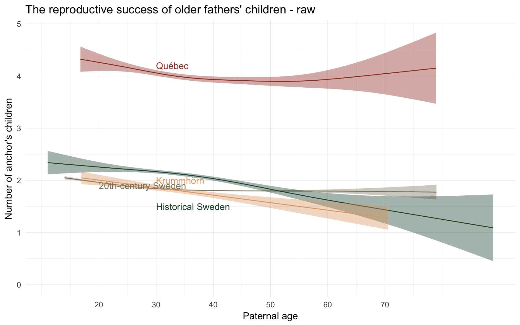
rm(populations)m1: No sibling comparison
Marginal effect plot
model_name = "m1_children_linear_noranef"
m1 = bind_rows(
    "Krummhörn" = get_paternalage_effect(model_name, "krmh"),
    "Québec" = get_paternalage_effect(model_name, "rpqa"),
    "20th-century Sweden" =  get_paternalage_effect(model_name, "swed"),
    "Historical Sweden" = get_paternalage_effect(model_name, "ddb"),
.id = "Population"
)

m1_plot = ggplot(m1,  aes(x = paternalage*10, y = Estimate, colour = Population, fill = Population, ymin = lowerCI, ymax = upperCI)) +
    geom_smooth(stat = 'identity', position = position_identity()) +
#   geom_smooth(aes(colour = Population, weight = 1/Est.Error ,group = Population),method = "lm", se = F, lty = "dashed", position = position_identity()) +
    ggtitle("The reproductive success of older fathers' children - m1") +
  scale_y_continuous("Number of anchor's children", limits = c(0,NA))  +
    scale_x_continuous("Paternal age", breaks = c(20,30,40,50,60,70)) +
    analysis_theme +
    pop_colour + pop_fill +
annotate("text", label = "Québec", x = 30, y = 6.2, size = 8, colour = colour_values["Québec"], hjust = 0) +
    annotate("text", label = "20th-century Sweden", x = 30, y = 1.7, size = 8, colour = colour_values["20th-century Sweden"], hjust = 0) +
    annotate("text", label = "Historical Sweden", x = 30, y = 3, size = 8, colour = colour_values["Historical Sweden"], hjust = 0) +
    annotate("text", label = "Krummhörn", x = 72, y = 2, size = 8, colour = colour_values["Krummhörn"], hjust = 0) +
    theme(legend.position = c(-1,0),
                legend.justification = c(0,0))
m1_plot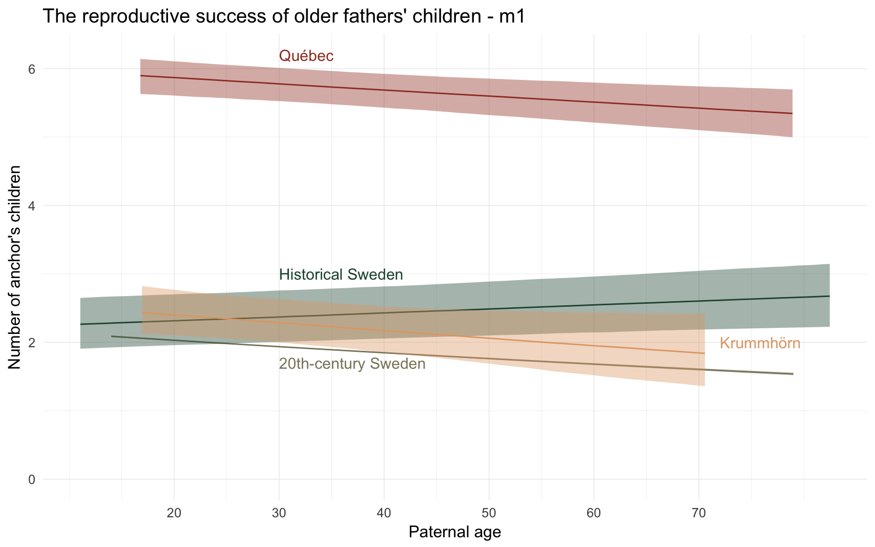
Effect size comparison
comp_plot(model_name)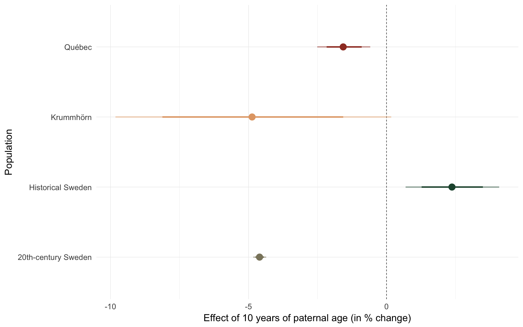
##            Population median_estimate         ci_95         ci_80
## 1           Krummhörn           -4.87 [-9.82; 0.17] [-8.12;-1.57]
## 2              Québec           -1.57 [-2.51;-0.59] [-2.17;-0.90]
## 3 20th-century Sweden           -4.60 [-4.83;-4.36] [-4.75;-4.44]
## 4 Historical Sweden 2.37 [0.69;4.08] [1.27;3.49]m3: Sibling comparison, linear paternal age effect
Marginal effect plot
model_name = "m3_children_linear"
m3 = bind_rows(
    "Krummhörn" = get_paternalage_effect(model_name, "krmh"),
    "Québec" = get_paternalage_effect(model_name, "rpqa"),
    "20th-century Sweden" =  get_paternalage_effect(model_name, "swed"),
    "Historical Sweden" = get_paternalage_effect(model_name, "ddb"),
.id = "Population"
)

m3_plot = ggplot(m3,  aes(x = paternalage*10, y = Estimate, colour = Population, fill = Population, ymin = lowerCI, ymax = upperCI)) +
    geom_smooth(stat = 'identity', position = position_identity()) +
#   geom_smooth(aes(colour = Population, weight = 1/Est.Error ,group = Population),method = "lm", se = F, lty = "dashed", position = position_identity()) +
    ggtitle("The reproductive success of older fathers' children - m3") +
  scale_y_continuous("Number of anchor's children", limits = c(0,NA))  +
    scale_x_continuous("Paternal age", breaks = c(20,30,40,50,60,70)) +
    analysis_theme +
    pop_colour + pop_fill +
annotate("text", label = "Québec", x = 30, y = 5, size = 8, colour = colour_values["Québec"], hjust = 0) +
    annotate("text", label = "20th-century Sweden", x = 15, y = 1.6, size = 8, colour = colour_values["20th-century Sweden"], hjust = 0) +
annotate("text", label = "Historical Sweden", x = 28, y = 3, size = 8, colour = colour_values["Historical Sweden"], hjust = 0) +
    annotate("text", label = "Krummhörn", x = 55, y = 0.5, size = 8, colour = colour_values["Krummhörn"], hjust = 0) +
    theme(legend.position = c(-1,0),
                legend.justification = c(0,0))
m3_plot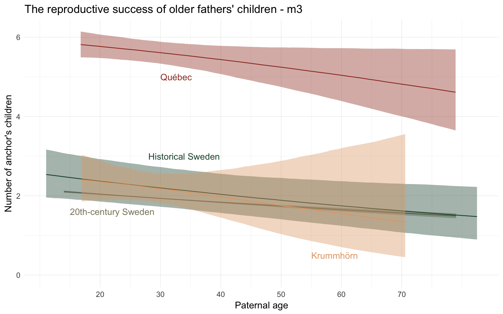
Effect size comparison
comp_plot(model_name)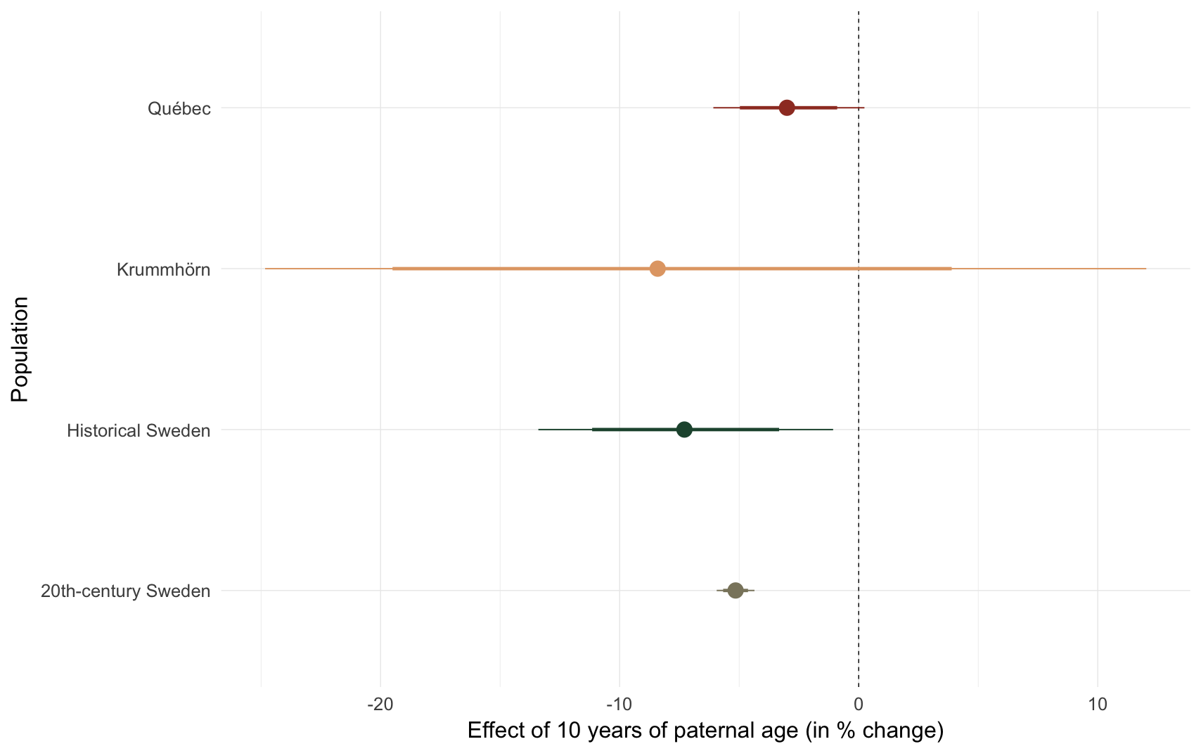
##            Population median_estimate           ci_95           ci_80
## 1           Krummhörn           -8.41 [-24.83; 12.03] [-19.50;  3.89]
## 2              Québec           -3.00   [-6.08; 0.24]   [-4.97;-0.90]
## 3 20th-century Sweden           -5.15   [-5.94;-4.36]   [-5.67;-4.63]
## 4 Historical Sweden -7.29 [-13.40; -1.07] [-11.15; -3.33]m4: Sibling comparison, nonlinear paternal age effect
Here, we test whether the paternal age effect is roughly linear by fitting a thin-plate spline.
Marginal effect plot
model_name = "m4_children_nonlinear"
m4 = bind_rows(
    "Krummhörn" = get_paternalage_effect(model_name, "krmh"),
    "Québec" = get_paternalage_effect(model_name, "rpqa"),
    "20th-century Sweden" =  get_paternalage_effect(model_name, "swed"),
    "Historical Sweden" = get_paternalage_effect(model_name, "ddb"),
.id = "Population"
)

m4_plot = ggplot(m4,  aes(x = paternalage*10, y = Estimate, colour = Population, fill = Population)) +
    geom_line(stat = 'identity', position = position_identity()) +
    geom_smooth(aes(colour = Population, weight = 1/Est.Error, group = Population),method = "lm", se = F, lty = "dashed", position = position_identity()) +
    ggtitle("The reproductive success of older fathers' children - m4") +
  scale_y_continuous("Number of anchor's children", limits = c(0,NA))  +
    xlab("Paternal age") +
    analysis_theme +
    pop_colour + pop_fill +
annotate("text", label = "Québec", x = 30, y = 5.2, size = 8, colour = colour_values["Québec"], hjust = 0) +
    annotate("text", label = "20th-century Sweden", x = 23, y = 1.6, size = 8, colour = colour_values["20th-century Sweden"], hjust = 0) +
annotate("text", label = "Historical Sweden", x = 25, y = 2.7, size = 8, colour = colour_values["Historical Sweden"], hjust = 0) +
    annotate("text", label = "Krummhörn", x = 50, y = 1.3, size = 8, colour = colour_values["Krummhörn"], hjust = 0) +  theme(legend.position = c(-1,0),
                legend.justification = c(0,0))
m4_plot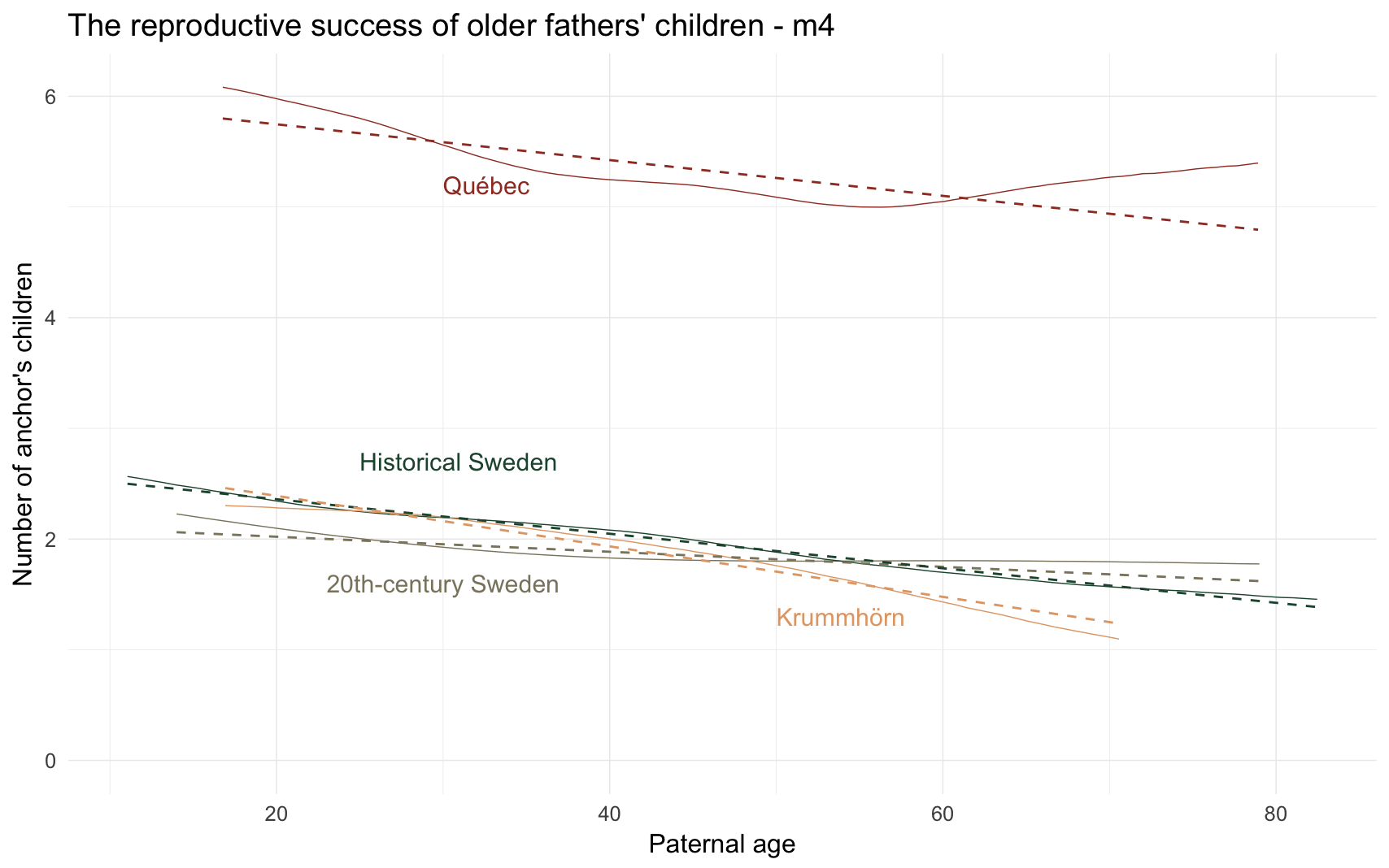
Alternative plot
m4_plot2 = ggplot(m4,  aes(x = paternalage*10, y = Estimate, colour = Population, fill = Population, ymin = lowerCI, ymax = upperCI)) +
    geom_smooth(stat = 'identity', position = position_identity()) +
    geom_smooth(aes(colour = Population, weight = 1/Est.Error, group = Population),method = "lm", se = F, lty = "dashed", position = position_identity(), alpha = 0.1) +
    ggtitle("The reproductive success of older fathers' children - m4") +
    scale_y_continuous("Number of anchor's children", breaks = scales::pretty_breaks(min.n = 2, n= 3))  +
    xlab("Paternal age") +
    analysis_theme +
    pop_colour + pop_fill +
    theme(legend.position = c(-1,0),legend.justification = c(0,0)) +
    facet_wrap(~ Population, nrow = 4, scales = 'free_y')
m4_plot2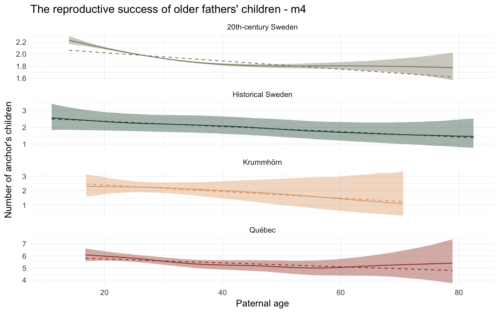
Effect size comparison
Compares children of 25 year-old fathers with those of 35-year-old fathers.
comp_plot(model_name)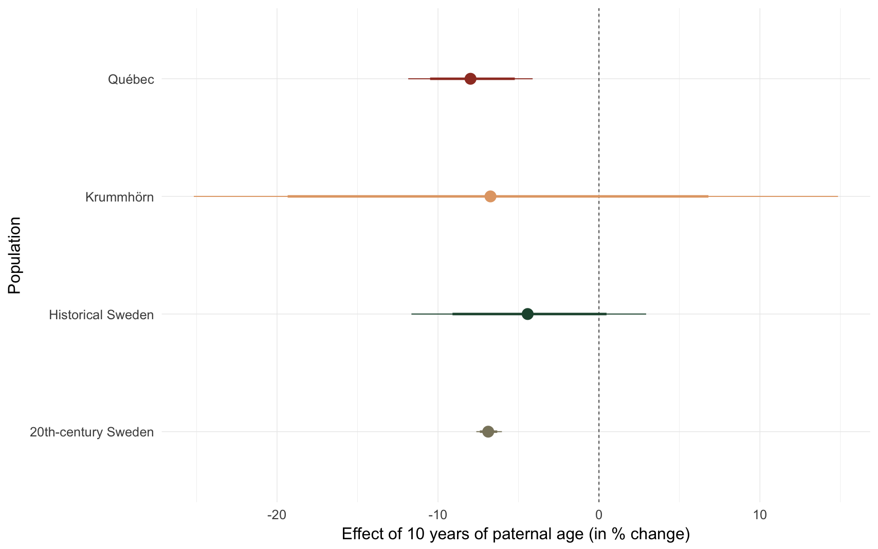
##            Population median_estimate           ci_95           ci_80
## 1           Krummhörn           -6.74 [-25.17; 14.85] [-19.34;  6.80]
## 2              Québec           -7.98 [-11.85; -4.12] [-10.49; -5.23]
## 3 20th-century Sweden           -6.88   [-7.62;-6.03]   [-7.40;-6.32]
## 4   Historical Sweden           -4.43 [-11.65;  2.93] [ -9.10;  0.47]