Comparing paternal age effects in our selective episode models
Loading details
source("0__helpers.R")
opts_chunk$set(warning=FALSE, cache=F,cache.lazy=F,tidy=FALSE,autodep=TRUE,dev=c('png','pdf'), fig.width=17.8,fig.height = 17.8*0.625,out.width='1440px',out.height='900px')e1: Survival to first year
Here, we predict the probability that the anchor survives the first year of life. All children born to this father are compared, if their death date is known or their survival can be inferred (from later marriage or children).
Marginal effect plot
episode = "e1_survive1y"
e1 = bind_rows(
    "Krummhörn" = get_paternalage_effect(episode, "krmh"),
    "Québec" = get_paternalage_effect(episode, "rpqa"),
    "20th-century Sweden" =  get_paternalage_effect(episode, "swed"),
    "Historical Sweden" = get_paternalage_effect(episode, "ddb"),
.id = "Population"
)

e1_plot = ggplot(e1,  aes(x = paternalage*10, y = Estimate, colour = Population, fill = Population, ymin = lowerCI, ymax = upperCI)) +
    geom_smooth(stat = 'identity', position = position_identity()) +
    ggtitle("Selective episode - e1") +
  scale_y_continuous("Probability of survival to first year", limits = c(0,1))  +
    scale_x_continuous("Paternal age", breaks = c(20,30,40,50,60,70)) +
    analysis_theme +
    pop_colour + pop_fill +
    theme(legend.position = c(0,0),
                legend.justification = c(0,0))
e1_plot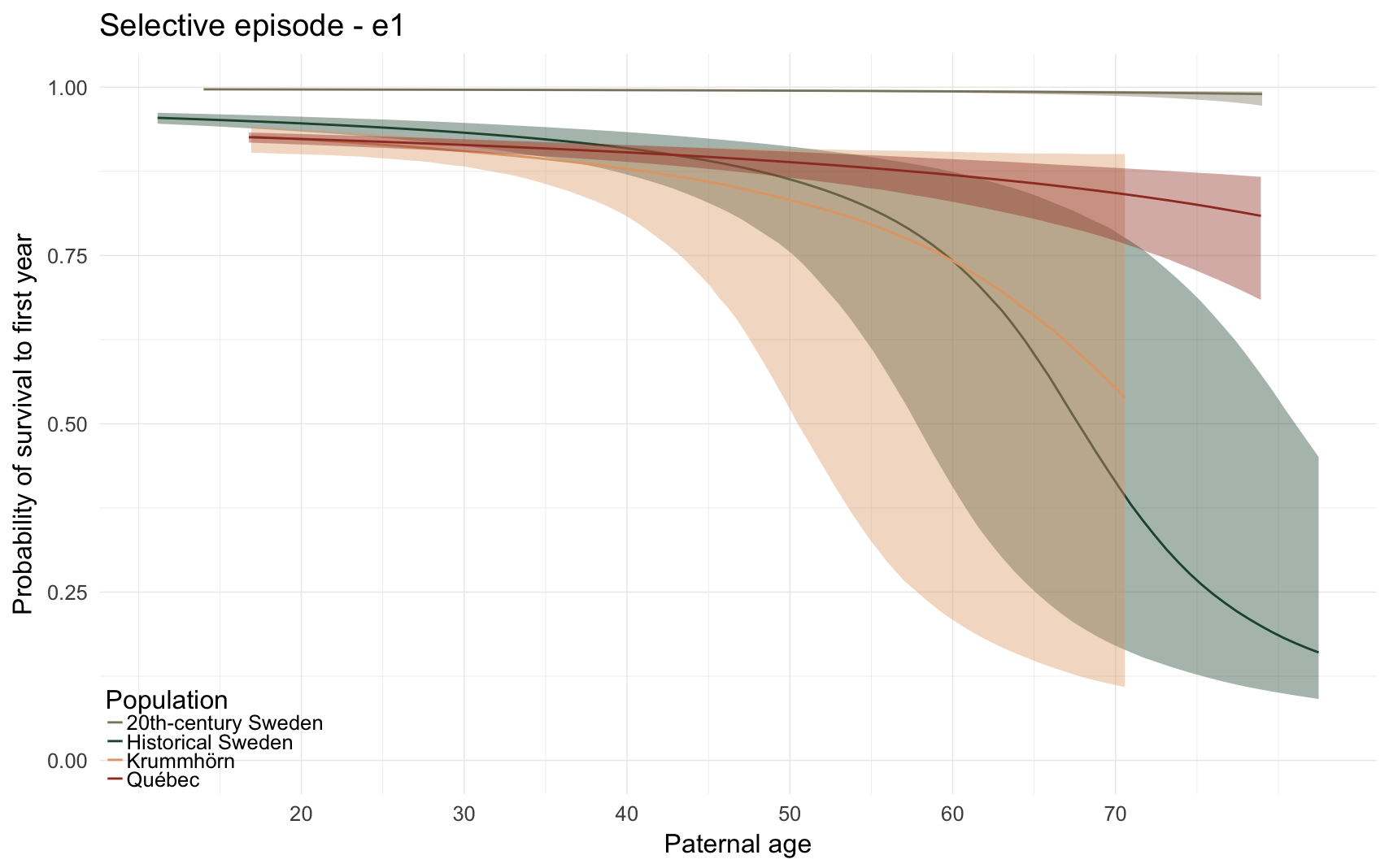
Effect size comparison
comp_plot(episode)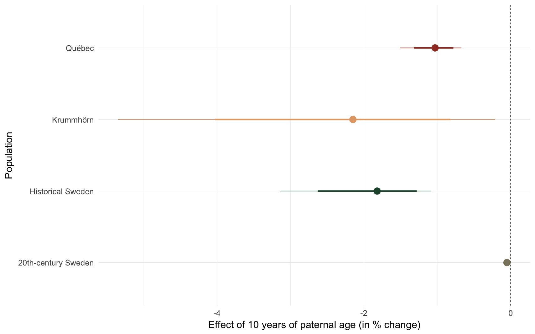
##            Population median_estimate         ci_95         ci_80
## 1           Krummhörn           -2.15 [-5.35;-0.21] [-4.03;-0.82]
## 2              Québec           -1.03 [-1.51;-0.67] [-1.32;-0.78]
## 3 20th-century Sweden           -0.05 [-0.06;-0.03] [-0.06;-0.03]
## 4 Historical Sweden -1.82 [-3.14;-1.08] [-2.63;-1.28]e2: Probability of surviving the first 15 years of life
Here, we predict the probability that the anchor survives the first fifteen of life. All children born to this father who lived at least one year are compared, if their death date is known or their survival can be inferred (from later marriage or children).
Marginal effect plot
episode = "e2_surviveR"
e2 = bind_rows(
    "Krummhörn" = get_paternalage_effect(episode, "krmh"),
    "Québec" = get_paternalage_effect(episode, "rpqa"),
    "20th-century Sweden" =  get_paternalage_effect(episode, "swed"),
    "Historical Sweden" = get_paternalage_effect(episode, "ddb"),
.id = "Population"
)

e2_plot = ggplot(e2,  aes(x = paternalage*10, y = Estimate, colour = Population, fill = Population, ymin = lowerCI, ymax = upperCI)) +
    geom_smooth(stat = 'identity', position = position_identity()) +
    ggtitle("Selective episode - e2") +
  scale_y_continuous("Probability of surviving to age 15", limits = c(0,1))  +
    scale_x_continuous("Paternal age", breaks = c(20,30,40,50,60,70)) +
    analysis_theme +
    pop_colour + pop_fill +
    theme(legend.position = c(0,0),
                legend.justification = c(0,0))
e2_plot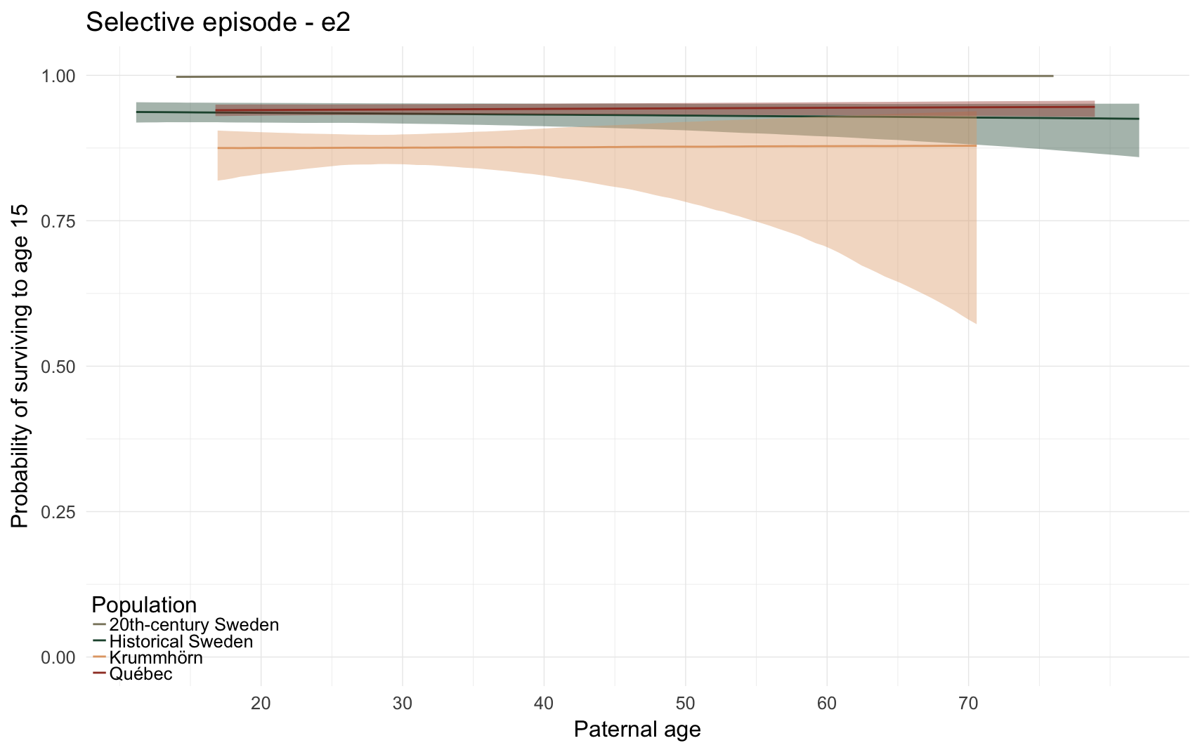
Effect size comparison
comp_plot(episode)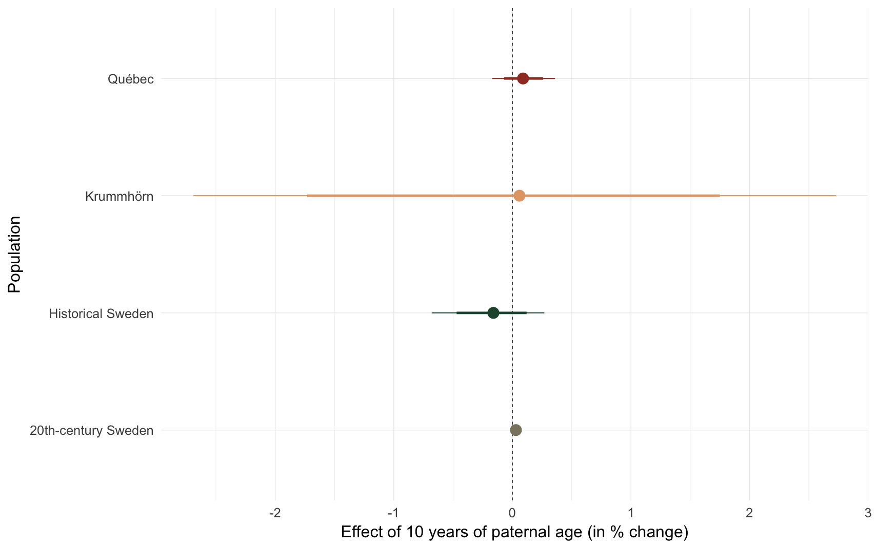
##            Population median_estimate         ci_95         ci_80
## 1           Krummhörn            0.06 [-2.69; 2.73] [-1.73; 1.75]
## 2              Québec            0.09 [-0.17; 0.36] [-0.07; 0.26]
## 3 20th-century Sweden            0.03   [0.00;0.06]   [0.01;0.05]
## 4 Historical Sweden -0.16 [-0.68; 0.27] [-0.47; 0.12]e3: Probability of ever marrying
Here, we predict the probability that the anchor ever marries. All anchors who reached reproductive age (15) are included.
Marginal effect plot
episode = "e3_ever_married"
e3 = bind_rows(
    "Krummhörn" = get_paternalage_effect(episode, "krmh"),
    "Québec" = get_paternalage_effect(episode, "rpqa"),
    "20th-century Sweden" =  get_paternalage_effect(episode, "swed"),
    "Historical Sweden" = get_paternalage_effect(episode, "ddb"),
.id = "Population"
)

e3_plot = ggplot(e3,  aes(x = paternalage*10, y = Estimate, colour = Population, fill = Population, ymin = lowerCI, ymax = upperCI)) +
    geom_smooth(stat = 'identity', position = position_identity()) +
    ggtitle("Selective episode - e3") +
  scale_y_continuous("Probability of ever marrying", limits = c(0,1))  +
    scale_x_continuous("Paternal age", breaks = c(20,30,40,50,60,70)) +
    analysis_theme +
    pop_colour + pop_fill +
    theme(legend.position = c(0,0),
                legend.justification = c(0,0))
e3_plot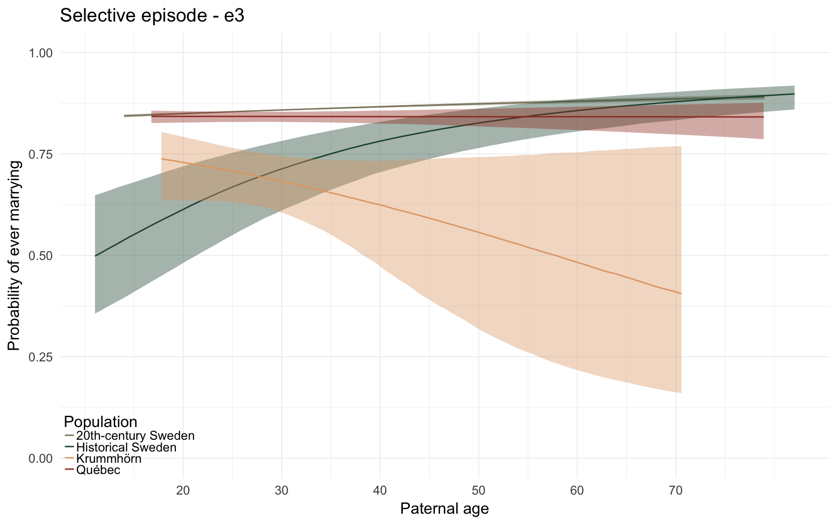
Effect size comparison
comp_plot(episode)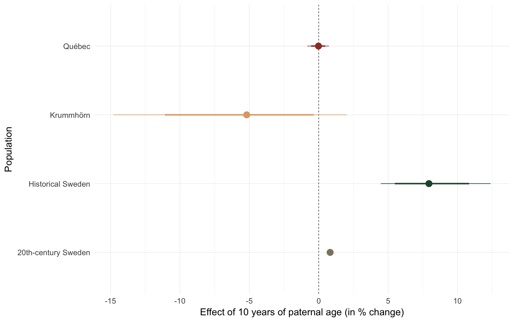
##            Population median_estimate           ci_95           ci_80
## 1           Krummhörn           -5.19 [-14.79;  2.01] [-11.08; -0.37]
## 2              Québec           -0.02   [-0.83; 0.74]   [-0.55; 0.46]
## 3 20th-century Sweden            0.82     [0.63;1.01]     [0.69;0.95]
## 4 Historical Sweden 7.94 [ 4.47;12.38] [ 5.48;10.83]e4: Number of children
Here, we predict the number of children that the anchor had. To separate this effect from previous selective episodes, we include only ever-married anchors and control for their number of spouses (interacted with sex, because men tend to have more additional children from further spouses).
Marginal effect plot
episode = "e4_children"
e4 = bind_rows(
    "Krummhörn" = get_paternalage_effect(episode, "krmh"),
    "Québec" = get_paternalage_effect(episode, "rpqa"),
    "20th-century Sweden" =  get_paternalage_effect(episode, "swed"),
    "Historical Sweden" = get_paternalage_effect(episode, "ddb"),
.id = "Population"
)

e4_plot = ggplot(e4,  aes(x = paternalage*10, y = Estimate, colour = Population, fill = Population, ymin = lowerCI, ymax = upperCI)) +
    geom_smooth(stat = 'identity', position = position_identity()) +
    ggtitle("Selective episode - e4") +
  scale_y_continuous("Probability of surviving to age 15", limits = c(0,NA))  +
    scale_x_continuous("Paternal age", breaks = c(20,30,40,50,60,70)) +
    analysis_theme +
    pop_colour + pop_fill +
    theme(legend.position = c(0,0.6),
                legend.justification = c(0,0))
e4_plot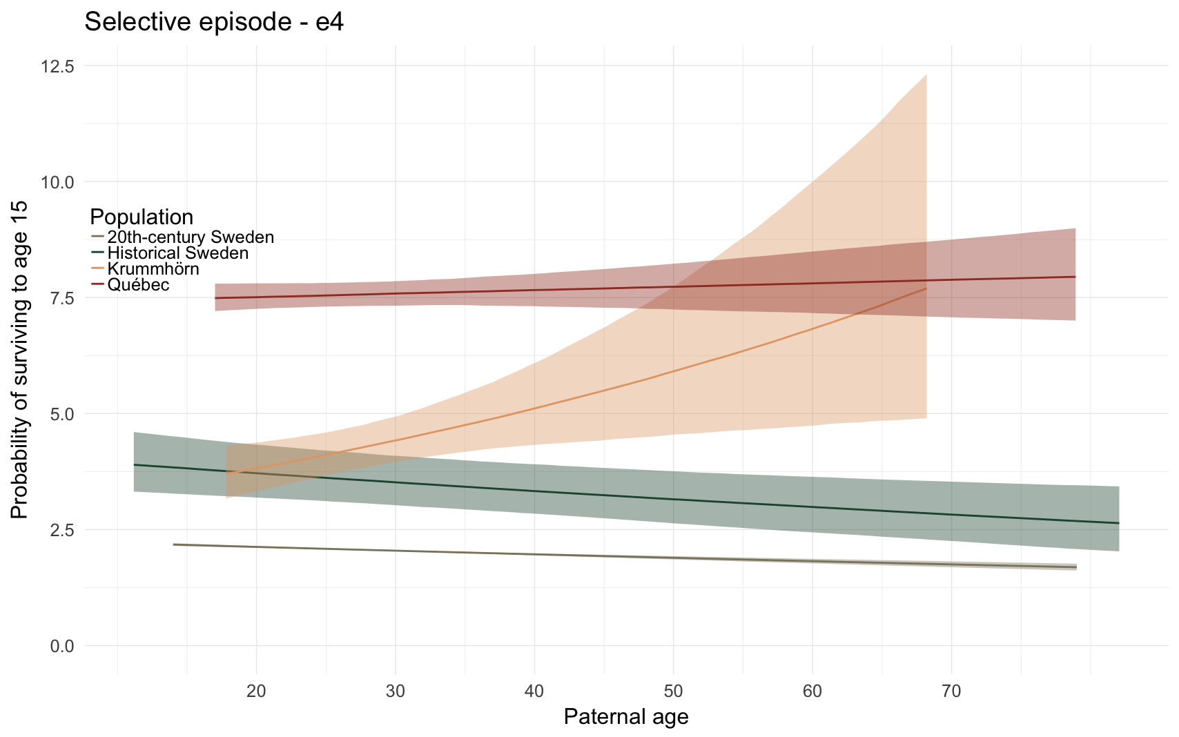
Effect size comparison
comp_plot(episode)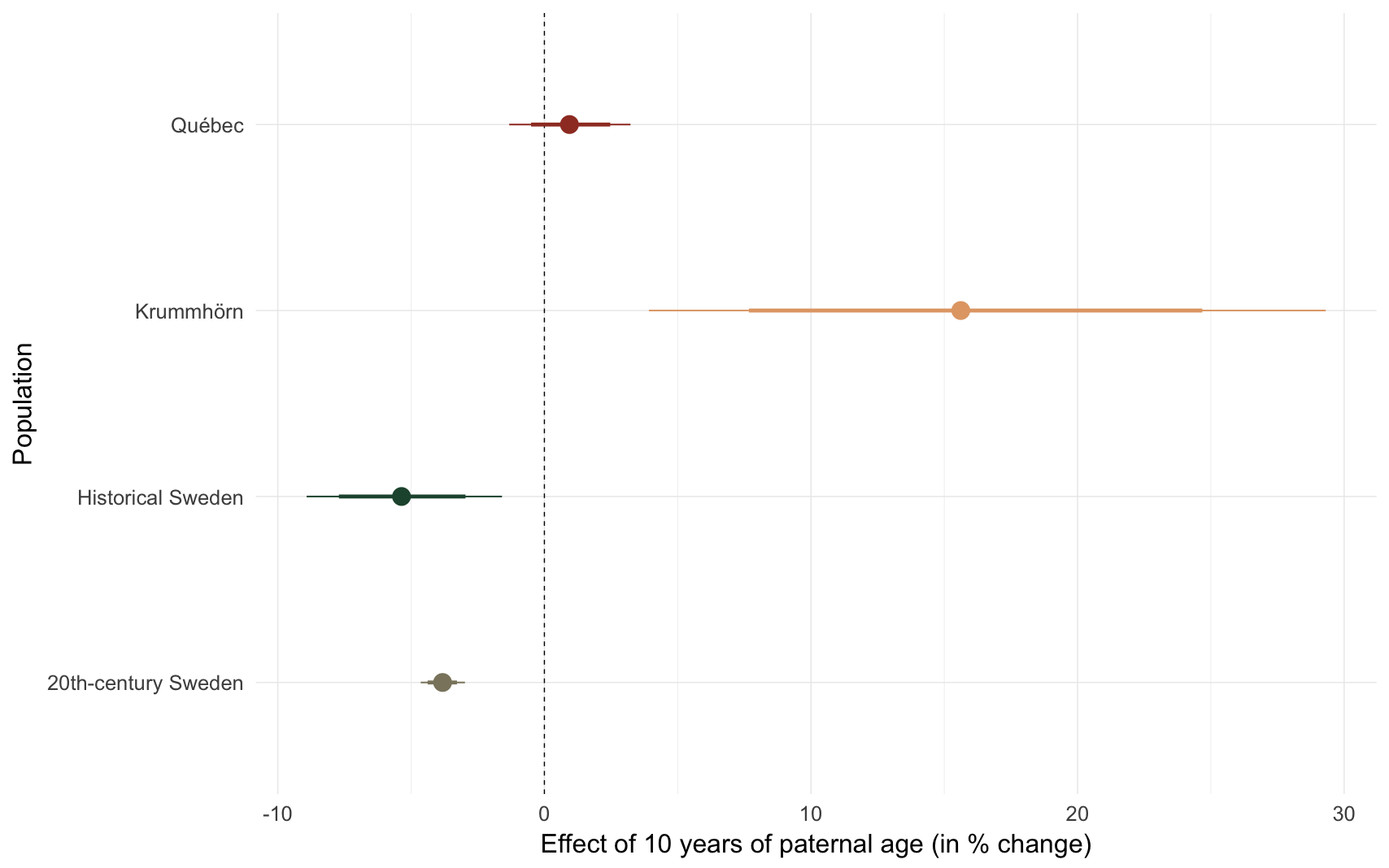
##            Population median_estimate         ci_95         ci_80
## 1           Krummhörn           15.62 [ 3.92;29.31] [ 7.67;24.68]
## 2              Québec            0.94 [-1.32; 3.23] [-0.50; 2.47]
## 3 20th-century Sweden           -3.82 [-4.64;-2.98] [-4.38;-3.28]
## 4   Historical Sweden           -5.36 [-8.92;-1.59] [-7.71;-2.96]
All episodes
paths = c("coefs/krmh/m3_children_linear.rds",
"coefs/rpqa/m3_children_linear.rds",
"coefs/ddb/m3_children_linear.rds",
"coefs/swed/m3_children_linear.rds",
list.files("coefs", full.names = TRUE, pattern = "^e._.+rds$", recursive = T))
i=1
effect_estimates = data.frame()
for (i in seq_along(paths)) {
filename = paths[i]
model = readRDS(paths[i])
if (class(model) == "brmsfit") {
chg = paternal_age_10y_effect(model)[3,]
chg$model = filename
chg$population = str_match(paths[i], "\\w+/(\\w+)/")[,2]
effect_estimates = rbind(chg, effect_estimates)
}
}
effect_estimates$episode = str_match(effect_estimates$model, "([em]\\d)_")[,2]
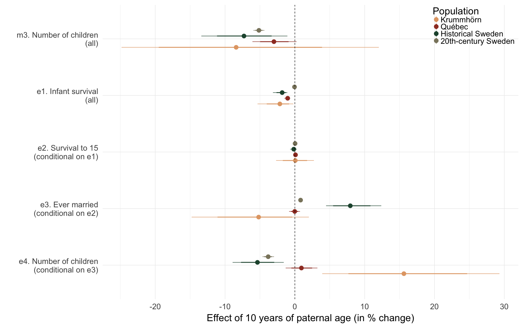
eps = c("m3" = 'm3. Number of children\n(all)',
"e1" = 'e1. Infant survival\n(all)',
"e2" = 'e2. Survival to 15\n(conditional on e1)',
"e3" = 'e3. Ever married\n(conditional on e2)',
"e4" = "e4. Number of children\n(conditional on e3)")
effect_estimates$episode = factor(eps[effect_estimates$episode], levels = rev(eps))
effect_estimates = effect_estimates %>% arrange(episode) %>%
mutate(
median_estimate = as.numeric(median_estimate),
lower95 = as.numeric(str_split_fixed(str_sub(ci_95, 2, -2), pattern = ';', 2)[,1]),
upper95 = as.numeric(str_split_fixed(str_sub(ci_95, 2, -2), pattern = ';', 2)[,2]),
lower80 = as.numeric(str_split_fixed(str_sub(ci_80, 2, -2), pattern = ';', 2)[,1]),
upper80 = as.numeric(str_split_fixed(str_sub(ci_80, 2, -2), pattern = ';', 2)[,2])
) -> effect_estimates
pops = c("krmh"='Krummhörn', "rpqa" = 'Québec', "ddb" = 'Historical Sweden', "swed" = '20th-century Sweden')
effect_estimates$Population = pops[effect_estimates$population]
effect_estimates$Population = factor(effect_estimates$Population, levels = pops)
episode_comparison = ggplot(effect_estimates %>% filter(!is.na(episode)), aes(x = factor(episode), y = median_estimate, ymin = lower95, ymax = upper95, color = Population)) +
geom_linerange(position = position_dodge(width = 0.4)) +
geom_pointrange(aes(ymin = lower80, ymax = upper80), size = 1, position = position_dodge(width = 0.4)) +
geom_hline(yintercept = 0, linetype = "dashed") +
scale_x_discrete("") +
pop_colour +
scale_y_continuous("Effect of 10 years of paternal age (in % change)") +
coord_flip() +
theme(legend.position = c(1,1),
legend.justification = c(1,1))
episode_comparison