Import
APA PsycTests
Show code
# A tibble: 1 × 2
  `n_distinct(Name)` `n()`
               <int> <int>
1               1237  3043
Show code
records_wide$first_construct <- str_trim(str_replace_all(str_to_lower(records_wide$first_construct), "[:space:]+", " "))Show code
psycinfo <- read_tsv('../sober_rubric/raw_data/merged_table_all.tsv') %>%
  # this tsv can be found in "Scraping-EBSCO-Host\data\merged tables"
#  mutate(Name = toTitleCase(Name)) %>%
  rename(usage_count = "Hit Count") %>%
  group_by(Name, Year) %>%
summarise(usage_count = sum(usage_count))Show code
[1] 31145[1] 40574Show code
nrow(overview)[1] 71692[1] 31118Show code
[1] 13280Show code
# for some few, the call was repeated by year for some reason
# one_hit_wonders %>% select(DOI, first_pub_year) %>% inner_join(byyear, by = "DOI") %>% arrange(DOI)

byyear <- byyear %>% anti_join(one_hit_wonders, by = "DOI")

all <- one_hit_wonders %>%
  select(DOI, Year, Hits) %>%
  bind_rows(byyear) %>%
  left_join(overview %>% rename(total_hits = Hits), by = "DOI")

n_distinct(all$DOI)
[1] 31145Show code
[1] 0Show code
[1] 0Show code
# all %>% group_by(total_hits, DOI) %>% summarise(hits_by_year = sum(usage_count, na.rm = T)) %>% filter(hits_by_year < total_hits) %>% select(DOI, everything()) %>% mutate(diff = hits_by_year - total_hits) %>%  View()
all %>% group_by(total_hits, DOI) %>% summarise(hits_by_year = sum(Hits, na.rm = T)) %>% filter(hits_by_year == total_hits) %>% nrow()
[1] 31118Show code
# A tibble: 27 × 2
   DOI                hits_by_year
   <chr>                     <dbl>
 1 10.1037/t00747-000            0
 2 10.1037/t00875-000            0
 3 10.1037/t00878-000            0
 4 10.1037/t00879-000            0
 5 10.1037/t02477-000            0
 6 10.1037/t02488-000            0
 7 10.1037/t04670-000            0
 8 10.1037/t04771-000            0
 9 10.1037/t04776-000            0
10 10.1037/t04779-000            0
# ℹ 17 more rows
Show code
.
 0
27
Show code
psyctests_info <- records_wide %>%
  select(DOI, TestYear, Name, first_construct,
         original_test_DOI, original_DOI_combined,
         test_type, ConstructList, subdiscipline_1, subdiscipline_2,
         classification_1, classification_2, instrument_type_broad,
         InstrumentType,
         number_of_factors_subscales, Name_base) %>%
  distinct() %>%
  inner_join(all, by = c("DOI" = "DOI"), multiple = "all") %>%
  rename(usage_count = "Hits")


write_rds(psyctests_info, "../sober_rubric/raw_data/psyctests_info.rds")
2016 changes in standards
Show code
test_data <- records_wide %>%
  filter(TestYear <= 2022) %>%
    rowwise() %>%
    mutate(Methodology = length(MethodologyList) >0) %>%
    mutate(AdministrationMethod = length(AdministrationMethodList) >0) %>%
    mutate(PopulationGroup = length(PopulationGroupList) >0) %>%
    mutate(AgeGroup = length(AgeGroupList) >0) %>%
    group_by(TestYear) %>%
    summarise(Reliability = mean(Reliability!="No reliability indicated."),
              FactorAnalysis = mean(FactorAnalysis!="No factor analysis indicated."),
              # Unidimensional = mean(FactorAnalysis=="This is a unidimensional measure."),
              FactorsAndSubscales = mean(!is.na(FactorsAndSubscales)),
              Validity = mean(Validity!="No validity indicated."),
              Format = mean(!is.na(Format)),
              # Fee = mean(Fee == "Yes"),
              Methodology = mean(Methodology),
              AdministrationMethod = mean(AdministrationMethod),
              # AgeGroup = mean(AgeGroup),
              # PopulationGroup = mean(PopulationGroup),
              TestItems = mean(TestItemsAvailable == "Yes")) %>%
    pivot_longer(-TestYear)
test_data %>%
  ggplot(aes(TestYear, value, color = name)) +
  geom_vline(xintercept = 2016, linetype = 'dashed') +
  geom_line() +
  scale_x_continuous("Publication year in APA PsycTests",
                     limits = c(1993, 2030),
                     breaks = seq(1993, 2022, by = 1),
                     labels = c(1993, "", "", "", "", 1998, "", "", "", "", 2003, "", "", "", "", 2008, "", "", "", "", 2013, "", "", "", "", 2018, "", "", "", "2022"),
                     expand = expansion(add = c(0, 1.2))) +
  scale_color_brewer(type = "qual", guide = "none", palette = 2) +
  geom_text_repel(
    data = test_data %>% drop_na() %>% group_by(name) %>% filter(TestYear == max(TestYear, na.rm = T)),
    aes(label = name),
    segment.color = 'grey',
    xlim = c(2022, 2033),
    box.padding = 0.1,
    # point.padding = 0.6,
    nudge_x = 1.2,
    # nudge_y = 0,
    force = 0.5,
    hjust = 0,
    direction="y",
    na.rm = TRUE
  ) +
  ylab("PsycTests contains information about...") +
  theme(panel.grid.minor.y = element_blank(),
        panel.grid.minor.x = element_blank(),
        plot.title.position = "plot",
        plot.title = element_text(face="bold"),
        legend.position = "none")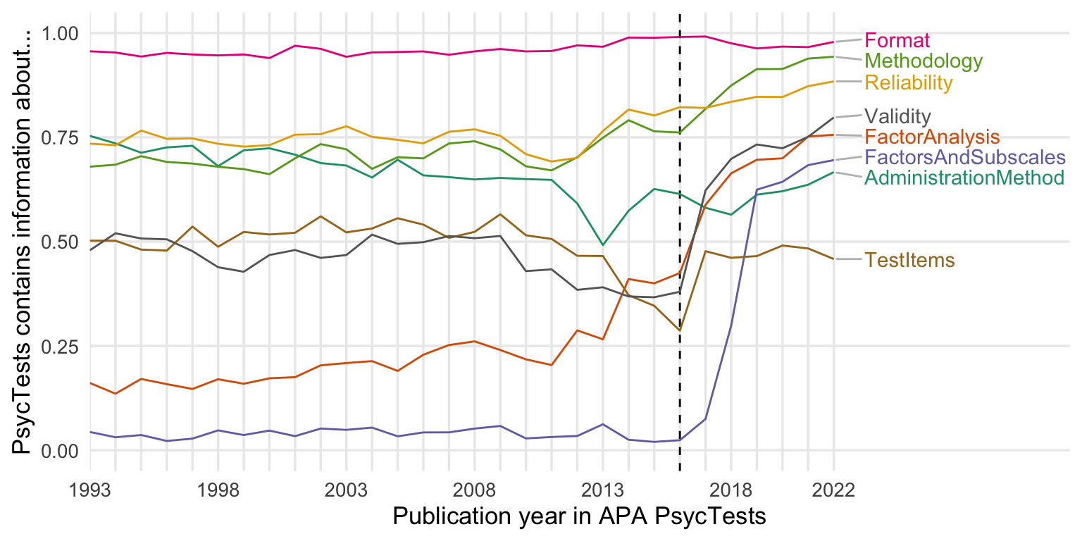
Show code
ggsave("figures/changed_standards_2016.pdf", width = 8, height = 4)
ggsave("figures/changed_standards_2016.png", width = 8, height = 4)
Show code
records_wide %>%
  group_by(TestYear) %>%
  summarise(number_of_test_items = mean(number_of_test_items, na.rm = T)) %>%
  filter(TestYear >= 1993, TestYear <= 2022) %>%
ggplot(aes(TestYear, number_of_test_items)) +
  geom_vline(xintercept = 2016, linetype = 'dashed') +
  geom_line() +
  scale_x_continuous("Publication year in APA PsycTests",
                     limits = c(1993, NA),
                     breaks = seq(1993, 2022, by = 1),
                     labels = c(1993, "", "", "", "", 1998, "", "", "", "", 2003, "", "", "", "", 2008, "", "", "", "", 2013, "", "", "", "", 2018, "", "", "", "2022")) +
  theme(panel.grid.minor.y = element_blank(),
        panel.grid.minor.x = element_blank(),
        plot.title.position = "plot",
        plot.title = element_text(face="bold"),
        legend.position = "none") +
  xlab("Publication year in APA PsycTests") +
  ylab("Number of items in measure")
Show code
records_wide %>%
  filter(TestYear >= 1993, TestYear <= 2022) %>%
ggplot(aes(TestYear, number_of_factors_subscales)) +
  geom_vline(xintercept = 2016, linetype = 'dashed') +
  geom_pointrange(stat = 'summary', fun.data = 'mean_se') +
  xlim(1993, 2022) +
  xlab("Publication year in APA PsycTests") +
  ylab("Number of factors/subscales")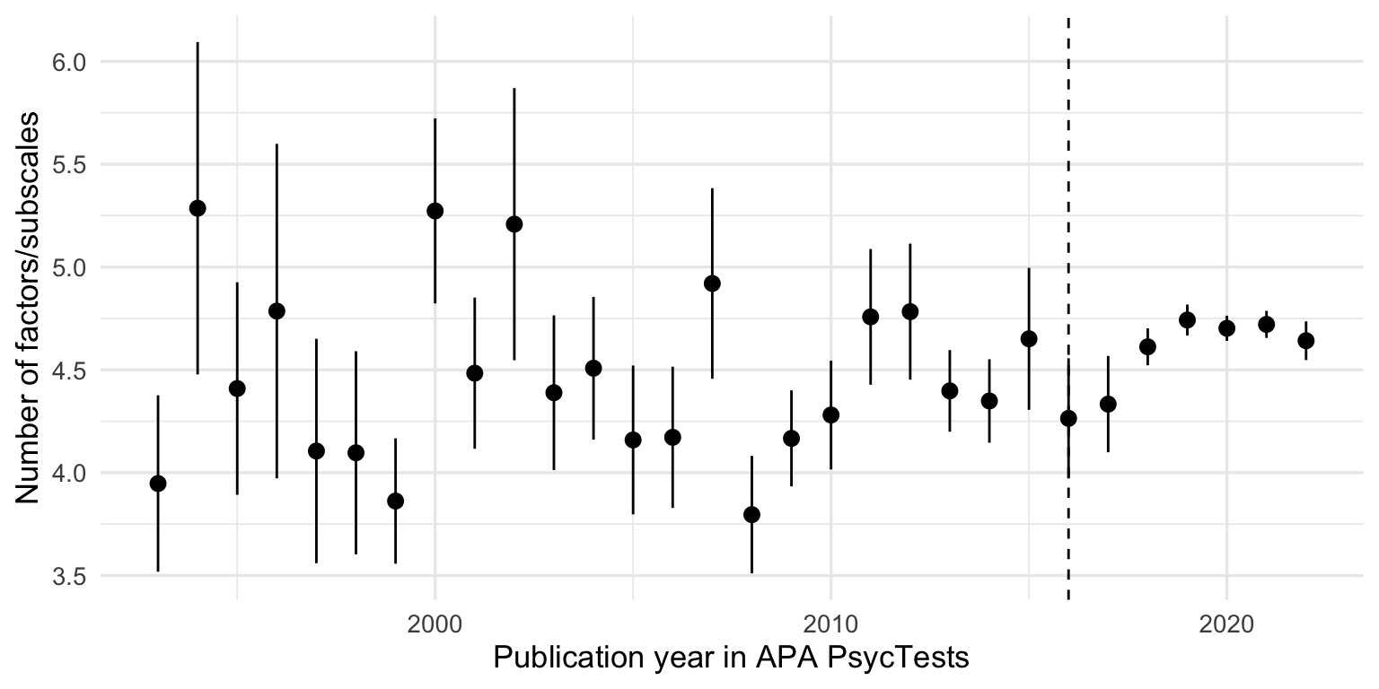
Show code
records_wide %>%
  group_by(InstrumentType, TestYear) %>%
  summarise(tests = n()) %>%
  group_by(TestYear) %>%
  mutate(tests = tests/sum(tests, na.rm = T)) %>%
  arrange(TestYear) %>%
  filter(TestYear >= 1993, TestYear <= 2022) %>%
  # mutate(tests = cumsum(tests)) %>%
  ggplot(aes(TestYear, tests, color = InstrumentType)) +
  geom_vline(xintercept = 2016, linetype = 'dashed') +
  scale_color_viridis_d() +
  geom_line() +
  xlim(1993, 2022) +
  xlab("Publication year in APA PsycTests") +
  ylab("Proportion of instrument type")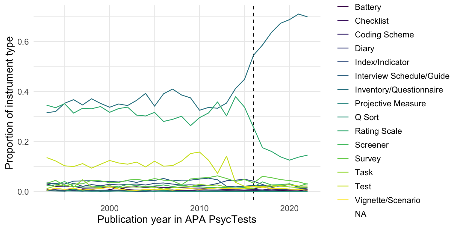
Show code
records_wide %>%
  # filter(instrument_type_broad !=)
  group_by(instrument_type_broad, TestYear) %>%
  summarise(tests = n()) %>%
  group_by(TestYear) %>%
  mutate(tests = tests/sum(tests, na.rm = T)) %>%
  arrange(TestYear) %>%
  filter(TestYear >= 1993, TestYear <= 2022) %>%
  # mutate(tests = cumsum(tests)) %>%
  ggplot(aes(TestYear, tests, color = instrument_type_broad)) +
  geom_vline(xintercept = 2016, linetype = 'dashed') +
  geom_line() +
  xlim(1993, 2022) +
  xlab("Publication year in APA PsycTests") +
  ylab("Proportion of instrument type")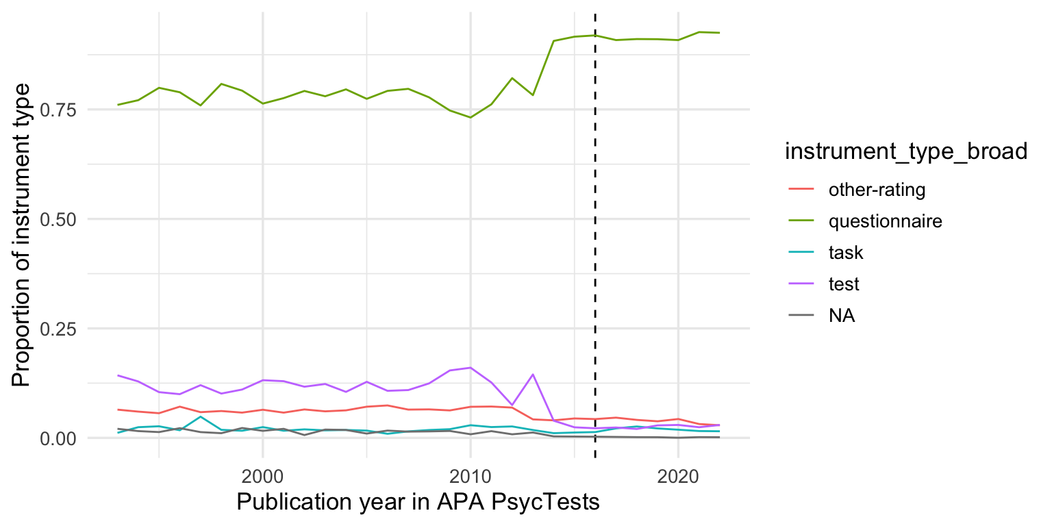
Show code
records_wide %>%
  filter(instrument_type_broad != "questionnaire") %>%
  group_by(InstrumentType, TestYear) %>%
  summarise(tests = n()) %>%
  group_by(TestYear) %>%
  mutate(tests = tests/sum(tests, na.rm = T)) %>%
  arrange(TestYear) %>%
  filter(TestYear >= 1993, TestYear <= 2022) %>%
  # mutate(tests = cumsum(tests)) %>%
  ggplot(aes(TestYear, tests, color = InstrumentType)) +
  geom_vline(xintercept = 2016, linetype = 'dashed') +
  geom_line() +
  xlim(1993, 2022) +
  xlab("Publication year in APA PsycTests") +
  ylab("Proportion of instrument type") +
  ggtitle("Without questionnaires")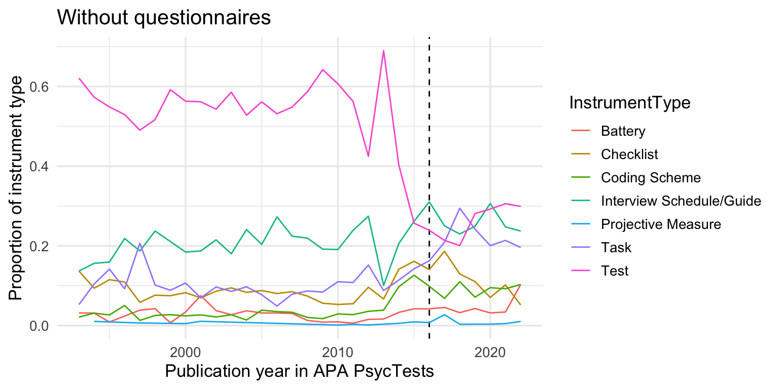
Show code
psyctests_info %>% group_by(DOI, TestYear) %>%
  summarise(used = sum(usage_count, na.rm = T)) %>%
  full_join(records_wide %>% select(DOI, TestYear)) %>%
  mutate(used = coalesce(used, 0)) %>%
  filter(TestYear >= 1993, TestYear <= 2022) %>%
  group_by(TestYear) %>%
  summarise(never_reused = mean(used == 0),
            used_once = mean(used == 1),
            used_twice = mean(used == 2),
            used_thrice = mean(used == 3),
            used_more_10 = mean(used > 9)) %>%
  pivot_longer(-TestYear) %>%
  ggplot(aes(TestYear, value, color = name)) +
  geom_vline(xintercept = 2016, linetype = 'dashed') +
  geom_line() +
  xlim(1993, 2022) +
  xlab("Publication year in APA PsycTests") +
  ylab("Frequency")
New measures by publication year
Show code
count_all <- records_wide %>%
  group_by(TestYear) %>%
  summarise(tests = n()) %>%
  arrange(TestYear)

count_orig <- records_wide %>%
  filter(test_type == "Original") %>%
  group_by(TestYear) %>%
  summarise(tests = n()) %>%
  arrange(TestYear)

count_base <- records_wide %>%
  arrange(TestYear) %>%
  distinct(Name_base, .keep_all = T) %>%
  group_by(TestYear) %>%
  summarise(tests = n_distinct(DOI))

count_construct <- records_wide %>%
  arrange(TestYear) %>%
  distinct(first_construct, .keep_all = T) %>%
  group_by(TestYear) %>%
  summarise(tests = n_distinct(first_construct)) %>%
  arrange(TestYear)

counts <- bind_rows(
  "novel constructs" = count_construct,
  "novel measures" = count_orig,
  "with translations\n and revisions" = count_all,
  .id = "origin"
  ) %>%
  rename(Year = TestYear) %>%
  filter(Year <= 2022)


ggplot(counts, aes(Year, tests, color = origin)) +
  geom_line() +
  geom_vline(xintercept = 2016, linetype = 'dashed') +
  scale_y_continuous("Number of measures/constructs published") +
  scale_x_continuous("Publication year in APA PsycTests",
                     limits = c(1993, 2030),
                     breaks = seq(1993, 2022, by = 1),
                     labels = c(1993, "", "", "", "", 1998, "", "", "", "", 2003, "", "", "", "", 2008, "", "", "", "", 2013, "", "", "", "", 2018, "", "", "", "2022")) +
  scale_color_brewer(type = "qual", guide = "none", palette = 2) +
  # ggrepel::geom_text_repel(
  #   aes(label = str_replace(subdiscipline, " Psychology", "")), data = entropy_by_year %>% filter(Year == max(Year, na.rm = T)),
  #   size = 4, hjust = 1,
  #   ) +
  geom_text_repel(data = counts %>% drop_na() %>% group_by(origin) %>% filter(Year == max(Year, na.rm = T)),
                  aes(label = paste0(" ", origin)),
                  segment.curvature = -0.1,
                  segment.square = TRUE,
                  lineheight = .9,
                  # segment.color = 'grey',
                  box.padding = 0.1,
                  point.padding = 0.6,
                  nudge_x = 1.5,
                  nudge_y = -15,
                  force = 1,
                  hjust = 0,
                  direction="y",
                  na.rm = F) +
   theme(panel.grid.minor.y = element_blank(),
        panel.grid.minor.x = element_blank(),
        plot.title.position = "plot",
        plot.title = element_text(face="bold"),
        legend.position = "none")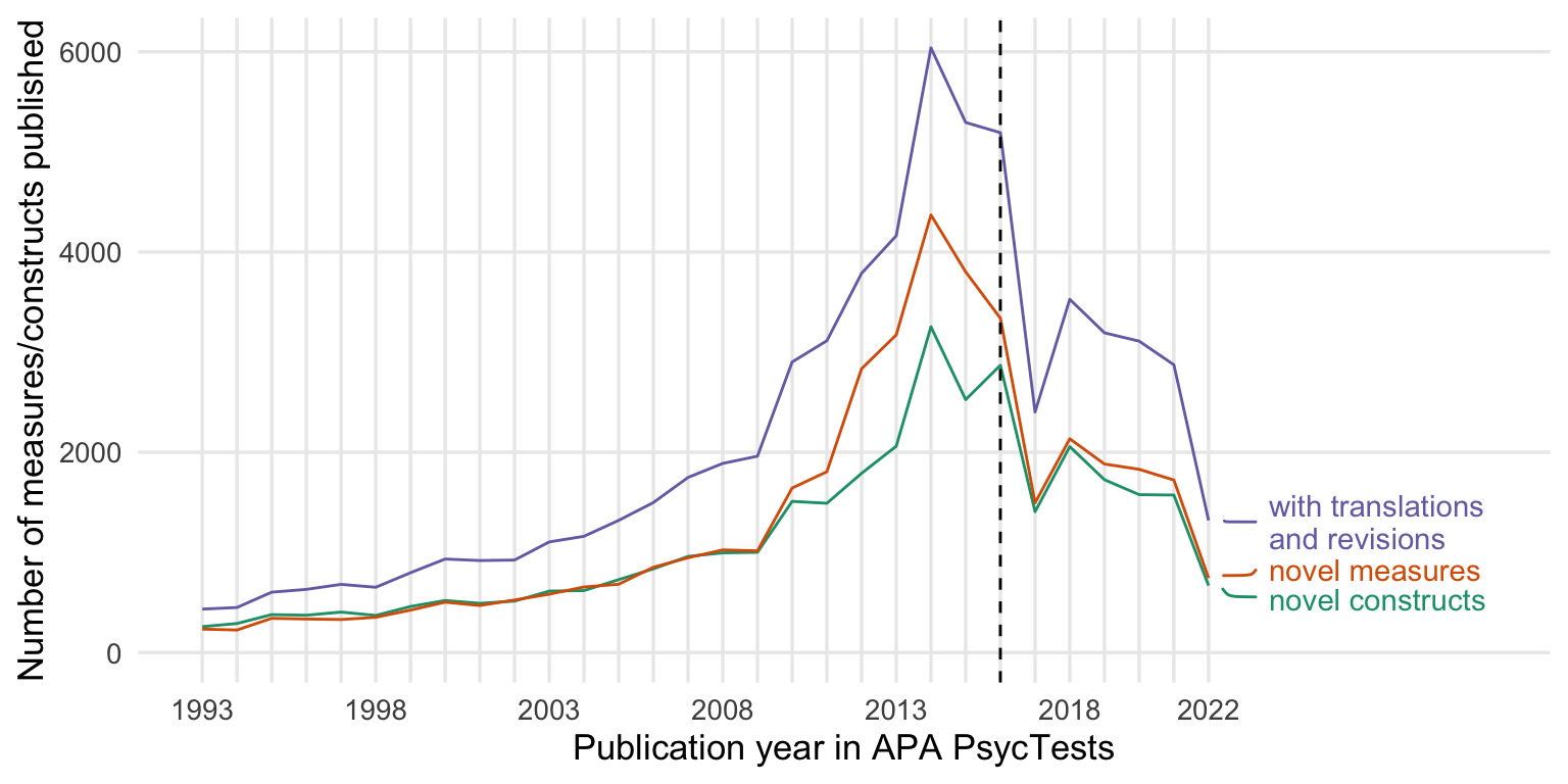
Show code
ggsave("figures/counts.pdf", width = 8, height = 4)
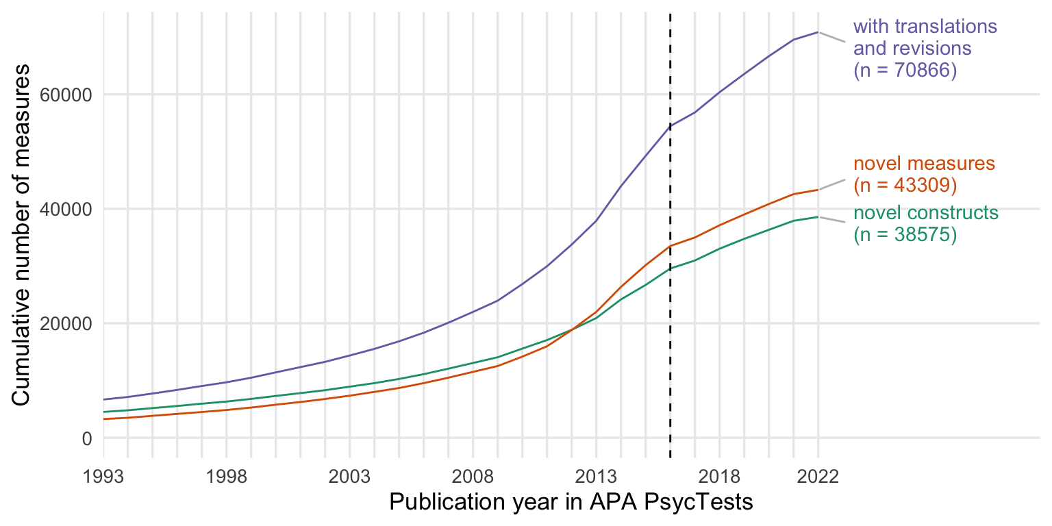
ggsave("figures/counts.png", width = 8, height = 4)Cumulative number of measures and constructs
Show code
cumsum_all <- records_wide %>%
  group_by(TestYear) %>%
  summarise(tests = n()) %>%
  arrange(TestYear) %>%
  mutate(tests = cumsum(tests))

cumsum_orig <- records_wide %>%
  filter(test_type == "Original") %>%
  group_by(TestYear) %>%
  summarise(tests = n()) %>%
  arrange(TestYear) %>%
  mutate(tests = cumsum(tests))

cumsum_base <- records_wide %>%
  arrange(TestYear) %>%
  distinct(Name_base, .keep_all = T) %>%
  group_by(TestYear) %>%
  summarise(tests = n_distinct(DOI)) %>%
  mutate(tests = cumsum(tests))

cumsum_construct <- records_wide %>%
  arrange(TestYear) %>%
  distinct(first_construct, .keep_all = T) %>%
  group_by(TestYear) %>%
  summarise(tests = n_distinct(DOI)) %>%
  arrange(TestYear) %>%
  mutate(tests = cumsum(tests))

cumsums <- bind_rows(
  "novel constructs" = cumsum_construct,
  "novel measures" = cumsum_orig,
  "with translations\n and revisions" = cumsum_all,
  .id = "origin"
  ) %>%
  rename(Year = TestYear) %>%
  filter(Year <= 2022)


ggplot(cumsums, aes(Year, tests, color = origin)) +
  geom_line() +
  geom_vline(xintercept = 2016, linetype = 'dashed') +
  scale_y_continuous("Cumulative number of measures") +
  scale_x_continuous("Publication year in APA PsycTests",
                     limits = c(1993, 2030),
                     breaks = seq(1993,2022, by = 1),
                     labels = c(1993, "", "", "", "", 1998, "", "", "", "", 2003, "", "", "", "", 2008, "", "", "", "", 2013, "", "", "", "", 2018, "", "", "", "2022"),
                     expand = expansion(add = c(0, 1))) +
  scale_color_brewer(type = "qual", guide = "none", palette = 2) +
  # ggrepel::geom_text_repel(
  #   aes(label = str_replace(subdiscipline, " Psychology", "")), data = entropy_by_year %>% filter(Year == max(Year, na.rm = T)),
  #   size = 4, hjust = 1,
  #   )  +
  geom_text_repel(data = cumsums %>% drop_na() %>% group_by(origin) %>% filter(Year == max(Year, na.rm = T)),
                  aes(label = paste0(" ", origin, "\n (n = ", tests, ")")),
                  segment.square = TRUE,
                  lineheight = .9,
                  segment.color = 'grey',
                  nudge_x = 1.2,
                  hjust = 0,
                  na.rm = TRUE) +
   # theme_minimal(base_size = 13) +
   theme(panel.grid.minor.y = element_blank(),
        panel.grid.minor.x = element_blank(),
        plot.title.position = "plot",
        plot.title = element_text(face="bold"),
        legend.position = "none")  +
    guides(
    x = guide_axis(cap = "both"), # Cap both ends
  )
Show code
ggsave("figures/cumsums.pdf", width = 8, height = 4)
ggsave("figures/cumsums.png", width = 8, height = 4)
By subdiscipline
Show code
cumsum_all <- records_wide %>%
  group_by(subdiscipline_1, TestYear) %>%
  summarise(tests = n()) %>%
  arrange(TestYear) %>%
  mutate(tests = cumsum(tests))


cumsum_orig <- records_wide %>%
  filter(test_type == "Original") %>%
  group_by(subdiscipline_1, TestYear) %>%
  summarise(tests = n()) %>%
  arrange(TestYear) %>%
  mutate(tests = cumsum(tests))

cumsum_base <- records_wide %>%
  arrange(TestYear) %>%
  distinct(Name_base, .keep_all = T) %>%
  group_by(subdiscipline_1, TestYear) %>%
  summarise(tests = n_distinct(DOI)) %>%
  mutate(tests = cumsum(tests))

cumsum_construct <- records_wide %>%
  arrange(TestYear) %>%
  distinct(first_construct, .keep_all = T) %>%
  group_by(subdiscipline_1, TestYear) %>%
  summarise(tests = n_distinct(DOI)) %>%
  arrange(TestYear) %>%
  mutate(tests = cumsum(tests))

cumsums <- bind_rows(
  "constructs" = cumsum_construct,
  "measures" = cumsum_orig,
  "with translations & revisions" = cumsum_all,
  .id = "origin"
  ) %>%
  rename(Year = TestYear) %>%
  filter(Year <= 2022)

cumsums$origin <- factor(cumsums$origin, levels = c("with translations & revisions", "constructs", "measures"))
my_colors <- c("with translations & revisions" = "#7570B3",
               "constructs" = "#1B9E77",
               "measures" = "#D95F02")

ggplot(cumsums, aes(Year, tests, color = origin)) +
  geom_line() +
  facet_wrap(~ subdiscipline_1, scales = "free_y", ncol = 2) +
  scale_y_continuous("Cumulative number of measures") +
  scale_x_continuous("Publication year in APA PsycTests",
                     limits = c(1993, 2022),
                     breaks = seq(1993, 2022, by = 1),
                     labels = c(1993, "", "", "", "", 1998, "", "", "", "", 2003, "", "", "", "", 2008, "", "", "", "", 2013, "", "", "", "", 2018, "", "", "", "2022")) +
  scale_color_manual(values = my_colors, guide = guide_legend(title = NULL)) +
  theme_minimal(base_size = 13) +
  theme(panel.grid.minor.y = element_blank(),
        panel.grid.minor.x = element_blank(),
        plot.title.position = "plot",
        plot.title = element_text(face="bold"),
        legend.position = c(0.58, 0.08),
        legend.justification = c(0, 0),
        legend.box.just = "right",
        legend.text = element_text(size = 11))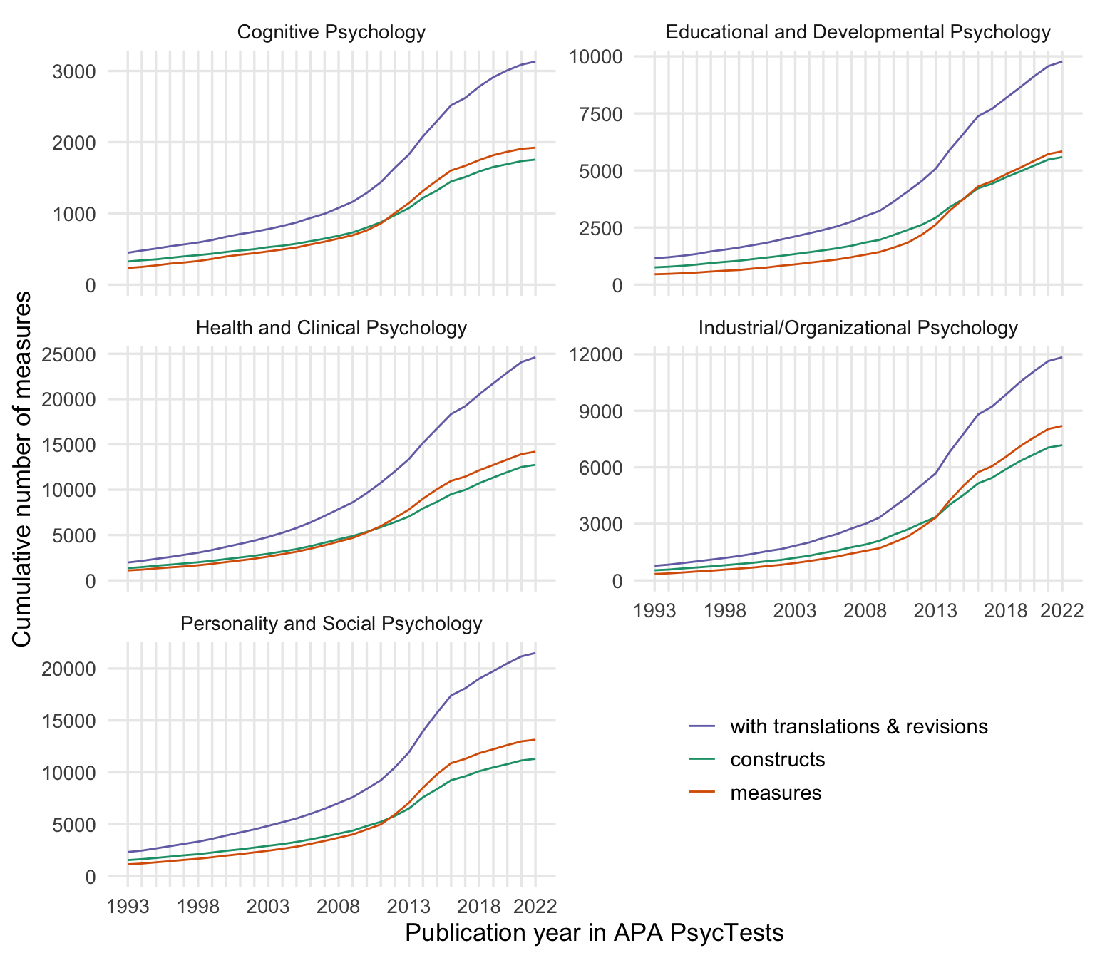
Show code
ggsave("figures/cumsums_subdiscipline.pdf", width = 8, height = 7)
ggsave("figures/cumsums_subdiscipline.png", width = 8, height = 7)
Tests by usage frequency
Show code
test_frequency <- psyctests_info %>%
  mutate(Test = if_else(test_type == "Original", DOI, original_test_DOI)) %>%
  drop_na(Test) %>%
  # filter(TestYear >= 1990) %>%
  filter(between(Year, 1993, 2022)) %>%
  group_by(Test) %>%
  summarise(n = sum(usage_count, na.rm = T)) %>%
  arrange(n)

test_frequency <- records_wide %>%
  filter(test_type == "Original", TestYear <= 2022) %>%
  select(Test = DOI) %>%
  full_join(test_frequency) %>%
  mutate(n = coalesce(n, 0.5))

test_frequency <- test_frequency %>%
  group_by(n) %>%
  summarise(count = n()) %>%
  ungroup() %>%
  mutate(percent = count/sum(count))

freq_plot <- ggplot(test_frequency, aes(n, count)) +
  geom_bar(width = 0.1, fill = colors["novel"], stat = "identity") +
  # facet_wrap(~ subdiscipline_1, scales = "free_y") +
  # scale_y_sqrt("Number of measures", breaks = c(0, 100, 400, 1000, 2000, 4000, 6000, 10000), limits = c(0, 11500)) +
  scale_y_continuous("Number of measures") +
  scale_x_log10("Usages recorded in APA PsycInfo 1993-2022",
                breaks = c(0.5, 1, 2, 5, 10, 100, 1000, 25000),
               labels = c(0, 1, 2, 5, 10, 100, 1000, 25000)) +

  geom_text(aes(label = if_else(n <= 2, sprintf("%.0f%%", percent*100), ""),
                x = n, y = count + 700)) +

  # scale_x_sqrt(breaks = c(0, 1, 2, 3, 4, 5, 10, 20, 40, 50), labels = c(0, 1, 2, 3, 4, 5, 10, 20, 40, "50+")) +
  # geom_text_repel(aes(x = n, label = first_acronym, y = y),
  #                 data =
  #                   test_frequency %>% group_by(subdiscipline_1) %>% filter(row_number() > (n() - 10) ) %>% left_join(records_wide %>% select(Test = DOI, first_acronym)) %>%
  #                   mutate(first_acronym = if_else(first_acronym == "HRSD", "HAM-D",
  #                                                  first_acronym)) %>%
    # mutate(y = 20 + 50*(1+n()-row_number())),
    #               size = 3.3, force = 5, force_pull  = 0, max.time = 1,
    #               max.overlaps = Inf,
    #               segment.color = "lightgray",
    #               segment.curvature = 1,
    #               hjust = 1,
    #               nudge_y = 10,
    #               direction = "y"
    # ) +
  theme_minimal(base_size = 13) +
  theme(panel.grid.minor.y = element_blank(),
        panel.grid.minor.x = element_blank(),
        plot.title.position = "plot",
        plot.title = element_text(face="bold"),
        legend.position = "none")
freq_plot
Show code
ggsave("figures/frequency_across.pdf", width = 8, height = 4)
ggsave("figures/frequency_across.png", width = 8, height = 4)

test_frequency <- test_frequency %>%
  filter(n >= 1) %>%
  mutate(percent = count/sum(count))

freq_plot <- ggplot(test_frequency, aes(n, count)) +
  geom_bar(width = 0.1, fill = colors["novel"], stat = "identity") +
  # scale_y_sqrt("Number of measures", breaks = c(0, 100, 400, 1000, 2000, 4000, 6000, 10000), limits = c(0, 11500)) +
  scale_y_continuous("Number of measures") +
  scale_x_log10("Usages recorded in APA PsycInfo 1993-2022",
                breaks = c(1, 2, 5, 10, 100, 1000, 25000),
               labels = c(1, 2, 5, 10, 100, 1000, 25000)) +

  geom_text(aes(label = if_else(n <= 2, sprintf("%.0f%%", percent*100), ""),
                x = n, y = count + 700)) +

  # scale_x_sqrt(breaks = c(0, 1, 2, 3, 4, 5, 10, 20, 40, 50), labels = c(0, 1, 2, 3, 4, 5, 10, 20, 40, "50+")) +
  # geom_text_repel(aes(x = n, label = first_acronym, y = y),
  #                 data =
  #                   test_frequency %>% group_by(subdiscipline_1) %>% filter(row_number() > (n() - 10) ) %>% left_join(records_wide %>% select(Test = DOI, first_acronym)) %>%
  #                   mutate(first_acronym = if_else(first_acronym == "HRSD", "HAM-D",
  #                                                  first_acronym)) %>%
    # mutate(y = 20 + 50*(1+n()-row_number())),
    #               size = 3.3, force = 5, force_pull  = 0, max.time = 1,
    #               max.overlaps = Inf,
    #               segment.color = "lightgray",
    #               segment.curvature = 1,
    #               hjust = 1,
    #               nudge_y = 10,
    #               direction = "y"
    # ) +
  theme_minimal(base_size = 13) +
  theme(panel.grid.minor.y = element_blank(),
        panel.grid.minor.x = element_blank(),
        plot.title.position = "plot",
        plot.title = element_text(face="bold"),
        legend.position = "none")
freq_plot
Show code
ggsave("figures/frequency_across_no0.pdf", width = 8, height = 4)
ggsave("figures/frequency_across_no0.png", width = 8, height = 4)
Show code
test_frequency <- psyctests_info %>%
  mutate(Test = if_else(test_type == "Original", DOI, original_test_DOI)) %>%
  drop_na(Test) %>%
  # filter(TestYear >= 1990) %>%
  filter(between(Year, 1993, 2022)) %>%
  group_by(subdiscipline_1, Test) %>%
  summarise(n = sum(usage_count, na.rm = T)) %>%
  arrange(n)

test_frequency <- records_wide %>%
  filter(test_type == "Original", TestYear <= 2022) %>%
  select(subdiscipline_1, Test = DOI) %>%
  full_join(test_frequency) %>%
  mutate(n = coalesce(n, 0.5))

test_frequency <- test_frequency %>%
  # mutate(n = if_else(n >= 1000, 1000, n)) %>%
  mutate(subdiscipline_1 = str_replace(subdiscipline_1, " Psychology", "")) %>%
  group_by(subdiscipline_1, n) %>%
  summarise(count = n()) %>%
  group_by(subdiscipline_1) %>%
  mutate(percent = count/sum(count))

freq_plot <- ggplot(test_frequency, aes(n, count)) +
  geom_bar(width = 0.1, fill = colors["novel"], stat = "identity") +
  facet_wrap(~ subdiscipline_1, scales = "free_y") +
  # scale_y_sqrt("Number of measures", breaks = c(0, 100, 400, 1000, 2000, 4000, 6000, 10000), limits = c(0, 11500)) +
  scale_y_continuous("Number of measures", expand = expansion(c(0, 0.1))) +
  scale_x_log10("Usages recorded in APA PsycInfo 1993-2022",
                breaks = c(0.5, 1, 2, 10, 100, 1000, 25000),
               labels = c(0, 1, 2, 10, 100, 1000, 25000)) +

  geom_text(aes(label = if_else(n <= 2, sprintf("%.0f%%", percent*100), ""),
                x = n, y = count ), size = 3, vjust = -0.4, hjust = 0.4) +

  # scale_x_sqrt(breaks = c(0, 1, 2, 3, 4, 5, 10, 20, 40, 50), labels = c(0, 1, 2, 3, 4, 5, 10, 20, 40, "50+")) +
  # geom_text_repel(aes(x = n, label = first_acronym, y = y),
  #                 data =
  #                   test_frequency %>% group_by(subdiscipline_1) %>% filter(row_number() > (n() - 10) ) %>% left_join(records_wide %>% select(Test = DOI, first_acronym)) %>%
  #                   mutate(first_acronym = if_else(first_acronym == "HRSD", "HAM-D",
  #                                                  first_acronym)) %>%
    # mutate(y = 20 + 50*(1+n()-row_number())),
    #               size = 3.3, force = 5, force_pull  = 0, max.time = 1,
    #               max.overlaps = Inf,
    #               segment.color = "lightgray",
    #               segment.curvature = 1,
    #               hjust = 1,
    #               nudge_y = 10,
    #               direction = "y"
    # ) +
  theme(panel.grid.minor.y = element_blank(),
        panel.grid.minor.x = element_blank(),
        plot.title.position = "plot",
        plot.title = element_text(face="bold"),
        legend.position = "none")

freq_plot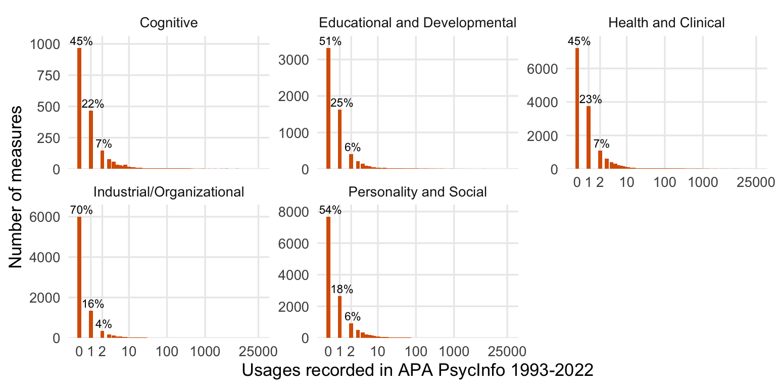
Show code
ggsave("figures/frequency.pdf", width = 8, height = 4)
ggsave("figures/frequency.png", width = 8, height = 4)

test_frequency <- test_frequency %>%
  filter(n >= 1) %>%
  group_by(subdiscipline_1) %>%
  mutate(percent = count/sum(count))

freq_plot <- ggplot(test_frequency, aes(n, count)) +
  geom_bar(width = 0.1, fill = colors["novel"], stat = "identity") +
  facet_wrap(~ subdiscipline_1, scales = "free_y") +
  # scale_y_sqrt("Number of measures", breaks = c(0, 100, 400, 1000, 2000, 4000, 6000, 10000), limits = c(0, 11500)) +
    scale_y_continuous("Number of measures", expand = expansion(c(0, 0.1))) +
  scale_x_log10("Usages recorded in APA PsycInfo 1993-2022",
                breaks = c(1, 2, 5, 10, 100, 1000, 25000),
               labels = c(1, 2, 5, 10, 100, 1000, 25000)) +

  geom_text(aes(label = if_else(n <= 2, sprintf("%.0f%%", percent*100), ""),
                x = n, y = count ), size = 3, vjust = -0.11, hjust = 0.4) +

  # scale_x_sqrt(breaks = c(0, 1, 2, 3, 4, 5, 10, 20, 40, 50), labels = c(0, 1, 2, 3, 4, 5, 10, 20, 40, "50+")) +
  # geom_text_repel(aes(x = n, label = first_acronym, y = y),
  #                 data =
  #                   test_frequency %>% group_by(subdiscipline_1) %>% filter(row_number() > (n() - 10) ) %>% left_join(records_wide %>% select(Test = DOI, first_acronym)) %>%
  #                   mutate(first_acronym = if_else(first_acronym == "HRSD", "HAM-D",
  #                                                  first_acronym)) %>%
    # mutate(y = 20 + 50*(1+n()-row_number())),
    #               size = 3.3, force = 5, force_pull  = 0, max.time = 1,
    #               max.overlaps = Inf,
    #               segment.color = "lightgray",
    #               segment.curvature = 1,
    #               hjust = 1,
    #               nudge_y = 10,
    #               direction = "y"
    # ) +
  theme(panel.grid.minor.y = element_blank(),
        panel.grid.minor.x = element_blank(),
        plot.title.position = "plot",
        plot.title = element_text(face="bold"),
        legend.position = "none")
freq_plot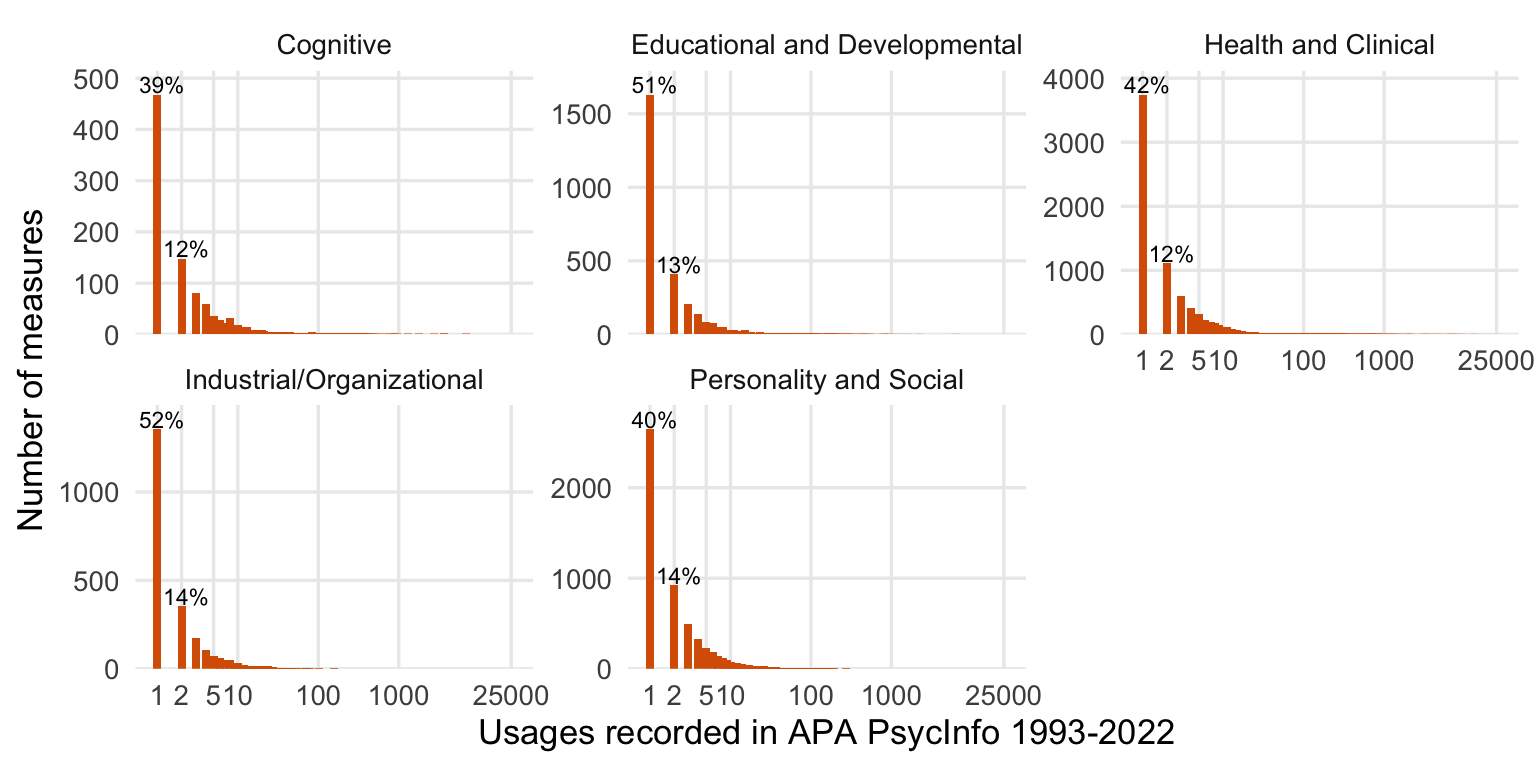
Show code
ggsave("figures/frequency_no0.pdf", width = 8, height = 4)By instrument type
Show code
usage_by_year_instrument_type <- psyctests_info %>%
  filter(between(Year, 1993, 2022)) %>%
  group_by(instrument_type_broad, Year, Test = DOI) %>%
  summarise(n = sum(usage_count, na.rm = T)) %>%
  group_by(instrument_type_broad) %>%
  mutate(n_tests = n_distinct(Test)) %>%
  group_by(instrument_type_broad, n_tests, Year) %>%
  summarise(n = sum(n),
            diff_tests = n()) %>%
  ungroup()


usage_by_year_instrument_type %>%
  ggplot(., aes(Year, n, color = instrument_type_broad)) +
  geom_line(size = 0.7) +
  scale_y_continuous("Times tests were coded in PsycInfo") +
  scale_x_continuous(limits = c(1993, 2030), breaks = c(1993, 1998, 2003, 2008, 2013, 2018, 2022)) +
  scale_color_brewer(type = "qual", guide = "none", palette = 2) +
  # ggrepel::geom_text_repel(
  #   aes(label = str_replace(subdiscipline, " Psychology", "")), data = entropy_by_year %>% filter(Year == max(Year, na.rm = T)),
  #   size = 4, hjust = 1,
  #   ) +
  geom_text_repel(aes(label = gsub("^.*$", " ", instrument_type_broad)), # This will force the correct position of the link's right end.
                  data = usage_by_year_instrument_type %>% filter(Year == max(Year, na.rm = T)),
                  segment.curvature = -0.1,
                  segment.square = TRUE,
                  segment.color = 'grey',
                  box.padding = 0.1,
                  point.padding = 0.6,
                  nudge_x = 0.15,
                  nudge_y = 0.05,
                  force = 0.5,
                  hjust = 0,
                  direction="y",
                  na.rm = TRUE
  ) +
  geom_text_repel(data = usage_by_year_instrument_type %>% filter(Year == max(Year, na.rm = T)),
                  aes(label = paste0("  ",str_replace(instrument_type_broad, " Psychology", ""), " (n=", n_tests, ")")),
                  segment.alpha = 0, ## This will 'hide' the link
                  segment.curvature = -0.1,
                  segment.square = TRUE,
                  # segment.color = 'grey',
                  box.padding = 0.1,
                  point.padding = 0.6,
                  nudge_x = 0.15,
                  nudge_y = 0.05,
                  force = 0.5,
                  hjust = 0,
                  direction="y",
                  na.rm = TRUE)+
  theme_minimal(base_size = 13) +
   theme(panel.grid.minor.y = element_blank(),
        panel.grid.minor.x = element_blank(),
        plot.title.position = "plot",
        plot.title = element_text(face="bold"),
        legend.position = "none")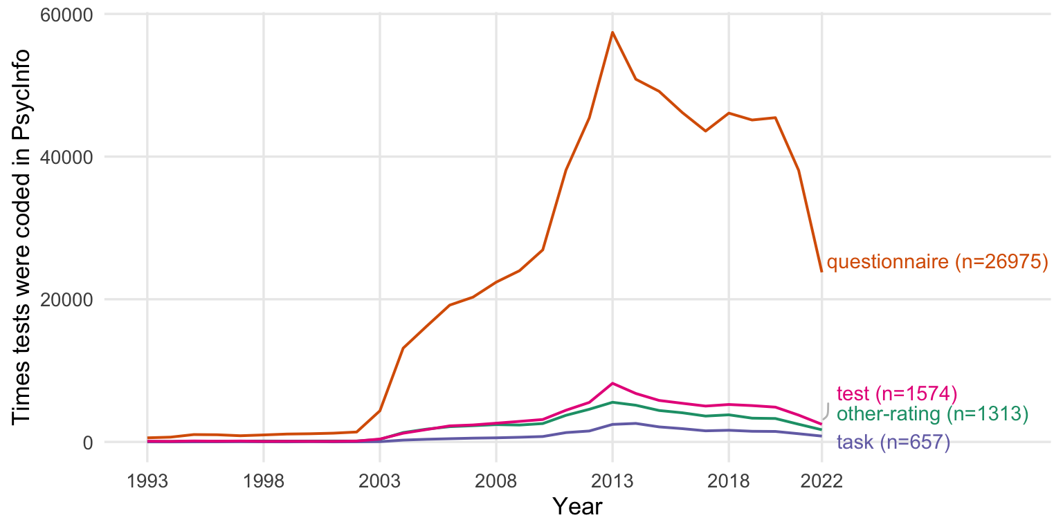
Show code
ggsave("figures/usage_by_year_instrument_type.pdf", width = 10, height = 4)
ggsave("figures/usage_by_year_instrument_type.png", width = 10, height = 4)
Show code
usage_by_year_instrument_type <- psyctests_info %>%
  filter(between(Year, 1993, 2022)) %>%
  group_by(InstrumentType, Year, Test = DOI) %>%
  summarise(n = sum(usage_count, na.rm = T)) %>%
  group_by(InstrumentType) %>%
  mutate(n_tests = n_distinct(Test)) %>%
  group_by(InstrumentType, n_tests, Year) %>%
  summarise(n = sum(n),
            diff_tests = n()) %>%
  ungroup()


usage_by_year_instrument_type %>%
  ggplot(., aes(Year, n, color = InstrumentType)) +
  geom_line(size = 0.7) +
  scale_y_continuous("Times tests were coded in PsycInfo") +
  scale_x_continuous(limits = c(1993, 2035), breaks = c(1993, 1998, 2003, 2008, 2013, 2018, 2022)) +
  scale_color_discrete() +
  # ggrepel::geom_text_repel(
  #   aes(label = str_replace(subdiscipline, " Psychology", "")), data = entropy_by_year %>% filter(Year == max(Year, na.rm = T)),
  #   size = 4, hjust = 1,
  #   ) +
  geom_text_repel(aes(label = gsub("^.*$", " ", InstrumentType)), # This will force the correct position of the link's right end.
                  data = usage_by_year_instrument_type %>% filter(Year == max(Year, na.rm = T)),
                  segment.curvature = -0.1,
                  segment.square = TRUE,
                  segment.color = 'grey',
                  box.padding = 0.1,
                  point.padding = 0.6,
                  nudge_x = 0.15,
                  nudge_y = 0.05,
                  force = 0.5,
                  hjust = 0,
                  direction="y",
                  na.rm = TRUE
  ) +
  geom_text_repel(data = usage_by_year_instrument_type %>% filter(Year == max(Year, na.rm = T)),
                  aes(label = paste0("  ",str_replace(InstrumentType, " Psychology", ""), " (n=", n_tests, ")")),
                  segment.alpha = 0, ## This will 'hide' the link
                  segment.curvature = -0.1,
                  segment.square = TRUE,
                  # segment.color = 'grey',
                  box.padding = 0.1,
                  point.padding = 0.6,
                  nudge_x = 0.15,
                  nudge_y = 0.05,
                  force = 0.5,
                  hjust = 0,
                  direction="y",
                  na.rm = TRUE)+
  theme_minimal(base_size = 13) +
   theme(panel.grid.minor.y = element_blank(),
        panel.grid.minor.x = element_blank(),
        plot.title.position = "plot",
        plot.title = element_text(face="bold"),
        legend.position = "none")
Show code
ggsave("figures/usage_by_year_instrument_type_narrow.pdf", width = 14, height = 10)
ggsave("figures/usage_by_year_instrument_type_narrow.png", width = 14, height = 10)
Entropy/Fragmentation
Show code
# searchstring:(TM *a* OR TM *e* OR TM *o* OR TM *i* OR TM *u*) AND PY "year (i.e. 1993)"
denominator <- rio::import("TnM_with_vowels_per_year_psycinfo.xlsx") %>%
  rename(Year = year, number_of_publications_with_tests_and_measures = results)
psyctests_info <- psyctests_info %>% left_join(denominator) %>%
    filter(between(Year, 1993, 2022))

var_label(psyctests_info$DOI) <- "Test DOI"
var_label(psyctests_info$TestYear) <- "When test was published according to PsycTests"
var_label(psyctests_info$first_pub_year) <- "First recorded year in which test was coded in PsycInfo"
var_label(psyctests_info$last_pub_year) <- "Last recorded year in which test was coded in PsycInfo"
var_label(psyctests_info$subdiscipline_1) <- "Subdiscipline of test"
var_label(psyctests_info$usage_count) <- "Frequency observed in PsycInfo"
write_rds(psyctests_info, "psycinfo_over_time.rds")
Revised approach using Hill diversity and coverage
Total number of tests coded in our scrape vs. total number of pubs with tests and measures are highly correlated. The former probably better represents sampling effort, because lower effort could also result in fewer tests being coded for a single paper. So, using the number of tests coded as our indicator of effort is proper.
Show code
pubs_vs_tests <- psyctests_info %>% group_by(Year) %>% summarise(n = sum(usage_count, na.rm = T), pubs_examined = mean(number_of_publications_with_tests_and_measures))
cor.test(pubs_vs_tests$n, pubs_vs_tests$pubs_examined) %>% broom::tidy() %>% knitr::kable(caption = "Correlation between publications with tests coded vs. number of tests per year")| estimate | statistic | p.value | parameter | conf.low | conf.high | method | alternative |
|---|---|---|---|---|---|---|---|
| 0.9791029 | 25.47591 | 0 | 28 | 0.9560829 | 0.9901174 | Pearson’s product-moment correlation | two.sided |
To compare across years, we use either rarefaction or coverage standardization to make every year directly comparable.
Show code
# Set a seed for reproducibility
set.seed(05102019)

### 1. Prepare Counts Data (example: All tests)
# Assume psyctests_info is already loaded and structured as in your original code.

counts_all <- psyctests_info %>%
  filter(between(Year, 1993, 2022)) %>%
  drop_na(DOI) %>%
  filter(usage_count > 0) %>%
  group_by(Year, Test = DOI) %>%
  summarise(n = sum(usage_count, na.rm = TRUE), .groups = "drop")

# 2.2. Revisions lumped
counts_lumped <- psyctests_info %>%
  filter(between(Year, 1993, 2022), usage_count > 0) %>%
  mutate(Test = if_else(test_type == "Original", DOI, original_test_DOI)) %>%
  drop_na(Test) %>%
  group_by(Year, Test) %>%
  summarise(n = sum(usage_count, na.rm = TRUE), .groups = "drop")

# 2.3. By construct
counts_construct <- psyctests_info %>%
  filter(between(Year, 1993, 2022), usage_count > 0) %>%
  drop_na(first_construct) %>%
  mutate(Test = first_construct) %>%
  group_by(Year, Test) %>%
  summarise(n = sum(usage_count, na.rm = TRUE), .groups = "drop")

### 2. Reshape Data: Make Tests the Rows and Years the Columns
# Pivot to wide format so that each row is a Test and each column (except Test) is a Year.
counts_all_wide <- counts_all %>%
  pivot_wider(id_cols = Test, names_from = Year, values_from = n, values_fill = list(n = 0))

counts_lumped_wide <- counts_lumped %>%
  pivot_wider(id_cols = Test, names_from = Year, values_from = n, values_fill = list(n = 0))

counts_construct_wide <- counts_construct %>%
  pivot_wider(id_cols = Test, names_from = Year, values_from = n, values_fill = list(n = 0))

### 3. Run iNEXT for Coverage-Based Comparison
# Here, we set q = 0 (species richness). You can set q = 1 for Hill–Shannon or q = 2 for Hill–Simpson.
inext_all <- iNEXT(counts_all_wide %>% tibble::column_to_rownames("Test"), q = 1, datatype = "abundance")
inext_lumped <- iNEXT(counts_lumped_wide %>% tibble::column_to_rownames("Test"), q = 1, datatype = "abundance")
inext_constructs <- iNEXT(counts_construct_wide %>% tibble::column_to_rownames("Test"), q = 1, datatype = "abundance")
Show code
inext_combined = bind_rows("all"  = inext_all$AsyEst, "lumped" = inext_lumped$AsyEst, "constructs" = inext_constructs$AsyEst, .id = "type") %>%
  mutate(Year = as.numeric(Assemblage)) %>%
  mutate(type = case_match(type,
                           "all" ~ "measures",
                           "constructs" ~ "constructs",
                            "lumped" ~ "with translations\n and revisions"))

ggplot(inext_combined, aes(x = Year, y = Estimator, ymin = LCL, ymax = UCL, group = type, color = type)) +
  geom_smooth(stat = "identity", size = 0.9) +
  facet_grid(Diversity ~ ., scales = "free_y") +
  scale_color_brewer(type = "qual", guide = "none", palette = 2) +
  theme_minimal(base_size = 14) +
  scale_x_continuous("Usage year as coded in APA PsycInfo", limits = c(1993, 2022),
                     breaks = seq(1993, 2022, by = 1),
                     labels = c(1993, "", "", "", "", 1998, "", "", "", "", 2003, "", "", "", "", 2008, "", "", "", "", 2013, "", "", "", "", 2018, "", "", "", "2022")) +
  labs(y = "Fragmentation index")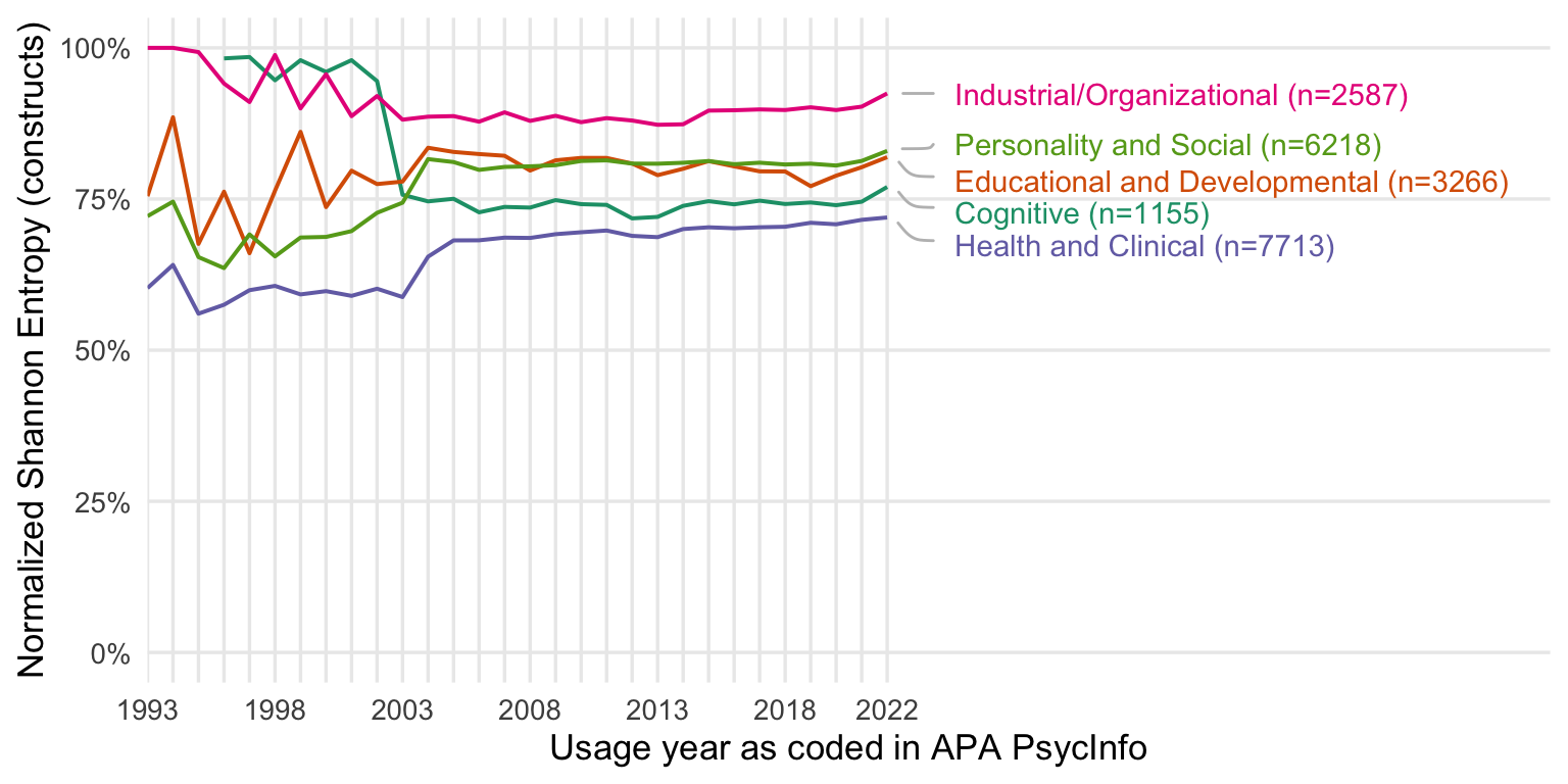
Show code
ggsave("figures/diversity_indices.pdf", width = 8, height = 6)
ggsave("figures/diversity_indices.png", width = 8, height = 6)
Show code
asymptotic_hill_shannon <- inext_combined %>% filter(Diversity %in% c( "Shannon diversity"))

asymptotic_hill_shannon %>%
  ggplot(., aes(Year, y = Estimator, min=LCL, ymax = UCL, color = type, fill = type)) +
  geom_smooth(size = 0.7, stat = "identity") +
  scale_y_continuous("Fragmentation index") +
  scale_x_continuous("Usage year as coded in APA PsycInfo", limits = c(1993, 2030),
                     breaks = seq(1993, 2022, by = 1),
                     labels = c(1993, "", "", "", "", 1998, "", "", "", "", 2003, "", "", "", "", 2008, "", "", "", "", 2013, "", "", "", "", 2018, "", "", "", "2022")) +
  scale_color_brewer(type = "qual", guide = "none", palette = 2) +
  scale_fill_brewer(type = "qual", guide = "none", palette = 2) +
  geom_vline(xintercept = 2016, linetype = 'dashed') +
  geom_text_repel(data = asymptotic_hill_shannon %>% drop_na() %>% group_by(type) %>% filter(Year == max(Year, na.rm = T)),
                  aes(label = paste0(" ",type)), # "\n (n = ", n_tests, ")"
                  segment.curvature = -0.5,
                  segment.square = TRUE,
                  segment.color = 'grey',
                  xlim = c(2023, 2030),
                  nudge_x = 1.14,
                  lineheight = .9,
                  hjust = 0,
                  direction="y",
                  na.rm = TRUE) +
  theme_minimal(base_size = 13) +
   theme(
        panel.grid.minor.y = element_blank(),
        panel.grid.minor.x = element_blank(),
        plot.title.position = "plot",
        plot.title = element_text(face="bold"),
        legend.position = "none")
Show code
ggsave("figures/entropy.pdf", width = 8, height = 4)
ggsave("figures/entropy.png", width = 8, height = 4)
By subdiscipline
Show code
# For each subdiscipline, pivot the counts (tests = DOI) across years, run iNEXT (q = 1),
# and extract the asymptotic Shannon diversity estimates.
asy_est_all_sub <- psyctests_info %>%
  filter(between(Year, 1993, 2022), usage_count > 0) %>%
  group_by(subdiscipline_1) %>%
  group_modify(~ {
    # Create a wide matrix: rows = tests (DOI), columns = Years
    counts <- .x %>%
      group_by(Year, Test = DOI) %>%
      summarise(n = sum(usage_count, na.rm = TRUE), .groups = "drop") %>%
      pivot_wider(id_cols = Test, names_from = Year, values_from = n, values_fill = list(n = 0))

    if(nrow(counts) > 0 && ncol(counts) > 1) {
      inext_obj <- iNEXT(counts %>% tibble::column_to_rownames("Test"), q = 1, datatype = "abundance")
      asy <- inext_obj$AsyEst %>%
        filter(Diversity == "Shannon diversity") %>%
        mutate(subdiscipline = .y$subdiscipline_1)
      asy
    } else {
      tibble()
    }
  }) %>%
  ungroup()

asy_est_all_sub <- asy_est_all_sub %>% rename(Year = Assemblage)
asy_est_all_sub %>%
  ggplot(., aes(x = as.numeric(Year), y = Estimator, color = subdiscipline)) +
  geom_line(size = 0.7) +
  scale_y_continuous("Fragmentation index") +
  scale_x_continuous("Usage year as coded in APA PsycInfo", limits = c(1993, 2033),
                     breaks = seq(1993,2022, by = 1),
                     labels = c(1993, "", "", "", "", 1998, "", "", "", "", 2003, "", "", "", "", 2008, "", "", "", "", 2013, "", "", "", "", 2018, "", "", "", "2022"),
                     expand = expansion(add = c(0, 7))) +
  scale_color_brewer(type = "qual", guide = "none", palette = 2) +
  # ggtitle(str_c(n_distinct(tests_by_year$Test), " measures tracked in PsycInfo")) +
 # geom_text_repel(aes(label = gsub("^.*$", " ", subdiscipline_1)), # This will force the correct position of the link's right end.
 #                  data = entropy_by_year %>% drop_na() %>% group_by(subdiscipline_1) %>% filter(Year == max(Year, na.rm = T)),
 #                  segment.curvature = -0.1,
 #                  segment.square = TRUE,
 #                  segment.color = 'grey',
 #                  box.padding = 0.1,
 #                  point.padding = 0.6,
 #                  max.overlaps = Inf,
 #                  nudge_x = 1.3,
 #                  # nudge_y = 0,
 #                  force = 20,
 #                  hjust = 0,
 #                  direction="y",
 #                  na.rm = TRUE
 #  ) +
  geom_text_repel(data = asy_est_all_sub %>% drop_na() %>% group_by(subdiscipline_1) %>% filter(Year == max(Year, na.rm = T)),
                  aes(label = paste0("  ",str_replace(subdiscipline_1, " Psychology", ""))),
                  # segment.alpha = 0, ## This will 'hide' the link
                  segment.curvature = -0.1,
                  segment.square = TRUE,
                  segment.color = 'grey',
                  box.padding = 0.1,
                  max.overlaps = Inf,
                  point.padding = 0.6,
                  xlim = c(2022, NA),
                  nudge_x = 2,
                  # nudge_y = 0.0,
                  force = 5,
                  hjust = 0,
                  direction="y",
                  na.rm = F) +
  theme_minimal(base_size = 13) +
  ggtitle("All measures, including revisions and translations") +
   theme(panel.grid.minor.y = element_blank(),
        panel.grid.minor.x = element_blank(),
        plot.title.position = "plot",
        plot.title = element_text(face="bold"),
        legend.position = "none") +
    coord_cartesian(clip = "off")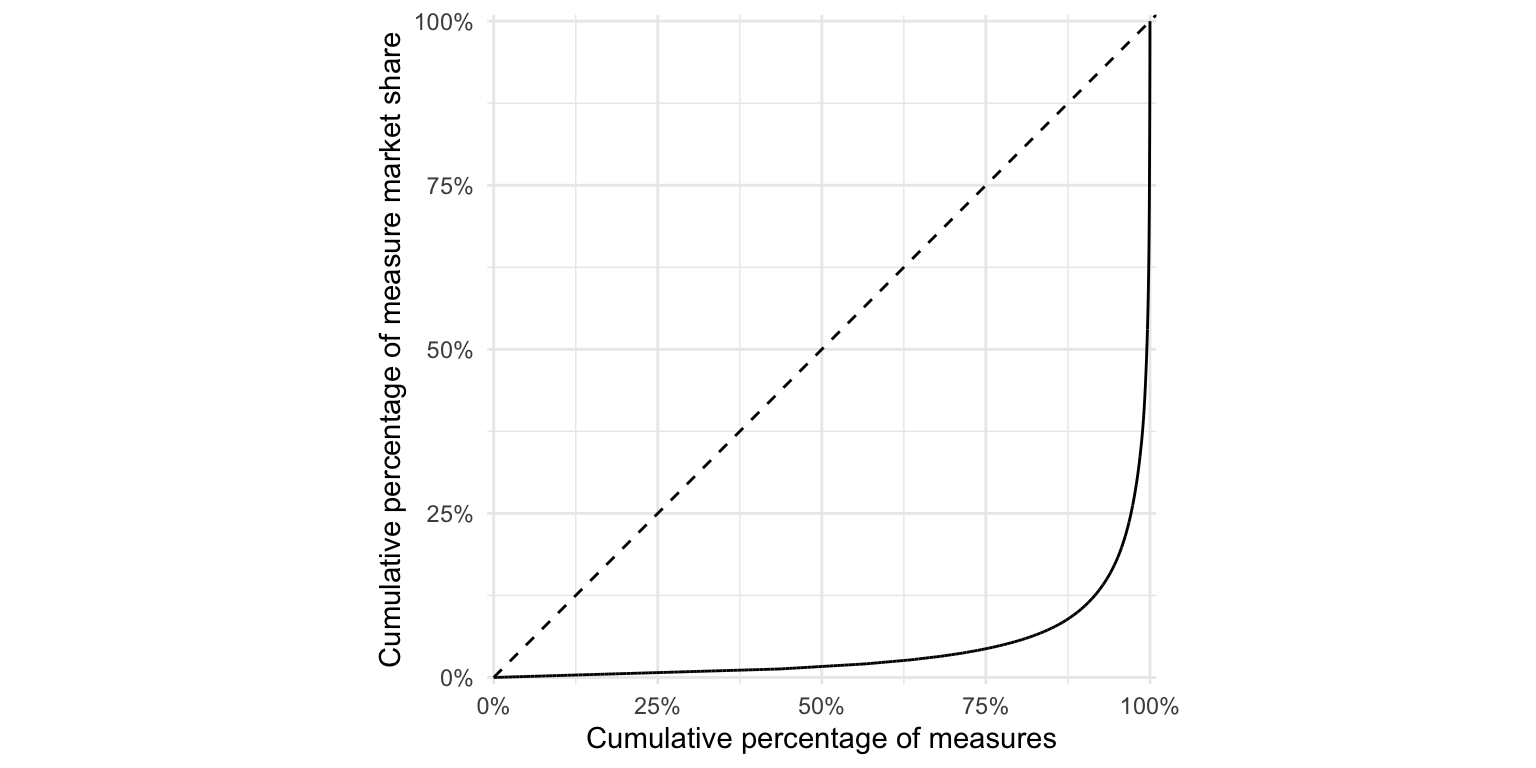
Show code
ggsave("figures/entropy_subdiscipline_all.pdf", width = 8, height = 4)
ggsave("figures/entropy_subdiscipline_all.png", width = 8, height = 4)
Show code
asy_est_orig_sub <- psyctests_info %>%
  filter(between(Year, 1993, 2022), usage_count > 0) %>%
  mutate(Test = if_else(test_type == "Original", DOI, original_test_DOI)) %>%
  drop_na(Test) %>%
  group_by(subdiscipline_1) %>%
  group_modify(~ {
    counts <- .x %>%
      group_by(Year, Test) %>%
      summarise(n = sum(usage_count, na.rm = TRUE), .groups = "drop") %>%
      pivot_wider(id_cols = Test, names_from = Year, values_from = n, values_fill = list(n = 0))

    if(nrow(counts) > 0 && ncol(counts) > 1) {
      inext_obj <- iNEXT(counts %>% tibble::column_to_rownames("Test"), q = 1, datatype = "abundance")
      asy <- inext_obj$AsyEst %>%
        filter(Diversity == "Shannon diversity") %>%
        mutate(subdiscipline = .y$subdiscipline_1)
      asy
    } else {
      tibble()
    }
  }) %>%
  ungroup()


asy_est_orig_sub <- asy_est_orig_sub %>% rename(Year = Assemblage)
asy_est_orig_sub %>%
  ggplot(., aes(x = as.numeric(Year), y = Estimator, color = subdiscipline)) +
  geom_line(size = 0.7) +
  scale_y_continuous("Fragmentation index") +
  scale_x_continuous("Usage year as coded in APA PsycInfo", limits = c(1993, 2033),
                     breaks = seq(1993,2022, by = 1),
                     labels = c(1993, "", "", "", "", 1998, "", "", "", "", 2003, "", "", "", "", 2008, "", "", "", "", 2013, "", "", "", "", 2018, "", "", "", "2022"),
                     expand = expansion(add = c(0, 7))) +
  scale_color_brewer(type = "qual", guide = "none", palette = 2) +
  # ggtitle(str_c(n_distinct(tests_by_year$Test), " measures tracked in PsycInfo")) +
 # geom_text_repel(aes(label = gsub("^.*$", " ", subdiscipline_1)), # This will force the correct position of the link's right end.
 #                  data = entropy_by_year %>% drop_na() %>% group_by(subdiscipline_1) %>% filter(Year == max(Year, na.rm = T)),
 #                  segment.curvature = -0.1,
 #                  segment.square = TRUE,
 #                  segment.color = 'grey',
 #                  box.padding = 0.1,
 #                  point.padding = 0.6,
 #                  max.overlaps = Inf,
 #                  nudge_x = 1.3,
 #                  # nudge_y = 0,
 #                  force = 20,
 #                  hjust = 0,
 #                  direction="y",
 #                  na.rm = TRUE
 #  ) +
  geom_text_repel(data = asy_est_orig_sub %>% drop_na() %>% group_by(subdiscipline_1) %>% filter(Year == max(Year, na.rm = T)),
                  aes(label = paste0("  ",str_replace(subdiscipline_1, " Psychology", ""))),
                  # segment.alpha = 0, ## This will 'hide' the link
                  segment.curvature = -0.1,
                  segment.square = TRUE,
                  segment.color = 'grey',
                  box.padding = 0.1,
                  max.overlaps = Inf,
                  point.padding = 0.6,
                  xlim = c(2022, NA),
                  nudge_x = 2,
                  # nudge_y = 0.0,
                  force = 5,
                  hjust = 0,
                  direction="y",
                  na.rm = F) +
  theme_minimal(base_size = 13) +
  ggtitle("Lumping revisions and translations with their originals") +
   theme(panel.grid.minor.y = element_blank(),
        panel.grid.minor.x = element_blank(),
        plot.title.position = "plot",
        plot.title = element_text(face="bold"),
        legend.position = "none") +
    coord_cartesian(clip = "off")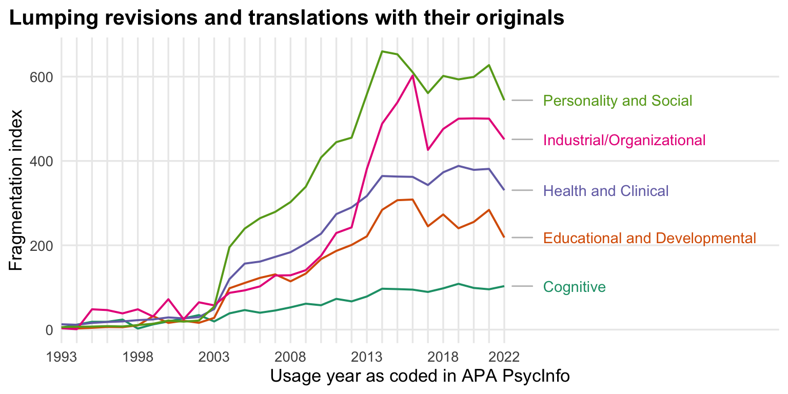
Show code
ggsave("figures/entropy_subdiscipline_orig.pdf", width = 8, height = 4)
ggsave("figures/entropy_subdiscipline_orig.png", width = 8, height = 4)
Show code
asy_est_constructs_sub <- psyctests_info %>%
  filter(between(Year, 1993, 2022), usage_count > 0) %>%
  group_by(subdiscipline_1) %>%
  group_modify(~ {
    counts <- .x %>%
      group_by(Year, Test = first_construct) %>%
      summarise(n = sum(usage_count, na.rm = TRUE), .groups = "drop") %>%
      pivot_wider(id_cols = Test, names_from = Year, values_from = n, values_fill = list(n = 0))

    if(nrow(counts) > 0 && ncol(counts) > 1) {
      inext_obj <- iNEXT(counts %>% tibble::column_to_rownames("Test"), q = 1, datatype = "abundance")
      asy <- inext_obj$AsyEst %>%
        filter(Diversity == "Shannon diversity") %>%
        mutate(subdiscipline = .y$subdiscipline_1)
      asy
    } else {
      tibble()
    }
  }) %>%
  ungroup()

asy_est_constructs_sub <- asy_est_constructs_sub %>% rename(Year = Assemblage)
asy_est_constructs_sub %>%
  ggplot(., aes(x = as.numeric(Year), y = Estimator, color = subdiscipline)) +
  geom_line(size = 0.7) +
  scale_y_continuous("Fragmentation index") +
  scale_x_continuous("Usage year as coded in APA PsycInfo", limits = c(1993, 2033),
                     breaks = seq(1993,2022, by = 1),
                     labels = c(1993, "", "", "", "", 1998, "", "", "", "", 2003, "", "", "", "", 2008, "", "", "", "", 2013, "", "", "", "", 2018, "", "", "", "2022"),
                     expand = expansion(add = c(0, 7))) +
  scale_color_brewer(type = "qual", guide = "none", palette = 2) +
  # ggtitle(str_c(n_distinct(tests_by_year$Test), " measures tracked in PsycInfo")) +
 # geom_text_repel(aes(label = gsub("^.*$", " ", subdiscipline_1)), # This will force the correct position of the link's right end.
 #                  data = entropy_by_year %>% drop_na() %>% group_by(subdiscipline_1) %>% filter(Year == max(Year, na.rm = T)),
 #                  segment.curvature = -0.1,
 #                  segment.square = TRUE,
 #                  segment.color = 'grey',
 #                  box.padding = 0.1,
 #                  point.padding = 0.6,
 #                  max.overlaps = Inf,
 #                  nudge_x = 1.3,
 #                  # nudge_y = 0,
 #                  force = 20,
 #                  hjust = 0,
 #                  direction="y",
 #                  na.rm = TRUE
 #  ) +
  geom_text_repel(data = asy_est_constructs_sub %>% drop_na() %>% group_by(subdiscipline_1) %>% filter(Year == max(Year, na.rm = T)),
                  aes(label = paste0("  ",str_replace(subdiscipline_1, " Psychology", ""))),
                  # segment.alpha = 0, ## This will 'hide' the link
                  segment.curvature = -0.1,
                  segment.square = TRUE,
                  segment.color = 'grey',
                  box.padding = 0.1,
                  max.overlaps = Inf,
                  point.padding = 0.6,
                  xlim = c(2022, NA),
                  nudge_x = 2,
                  # nudge_y = 0.0,
                  force = 5,
                  hjust = 0,
                  direction="y",
                  na.rm = F) +
  theme_minimal(base_size = 13) +
  ggtitle("All measures, including revisions and translations") +
   theme(panel.grid.minor.y = element_blank(),
        panel.grid.minor.x = element_blank(),
        plot.title.position = "plot",
        plot.title = element_text(face="bold"),
        legend.position = "none") +
    coord_cartesian(clip = "off")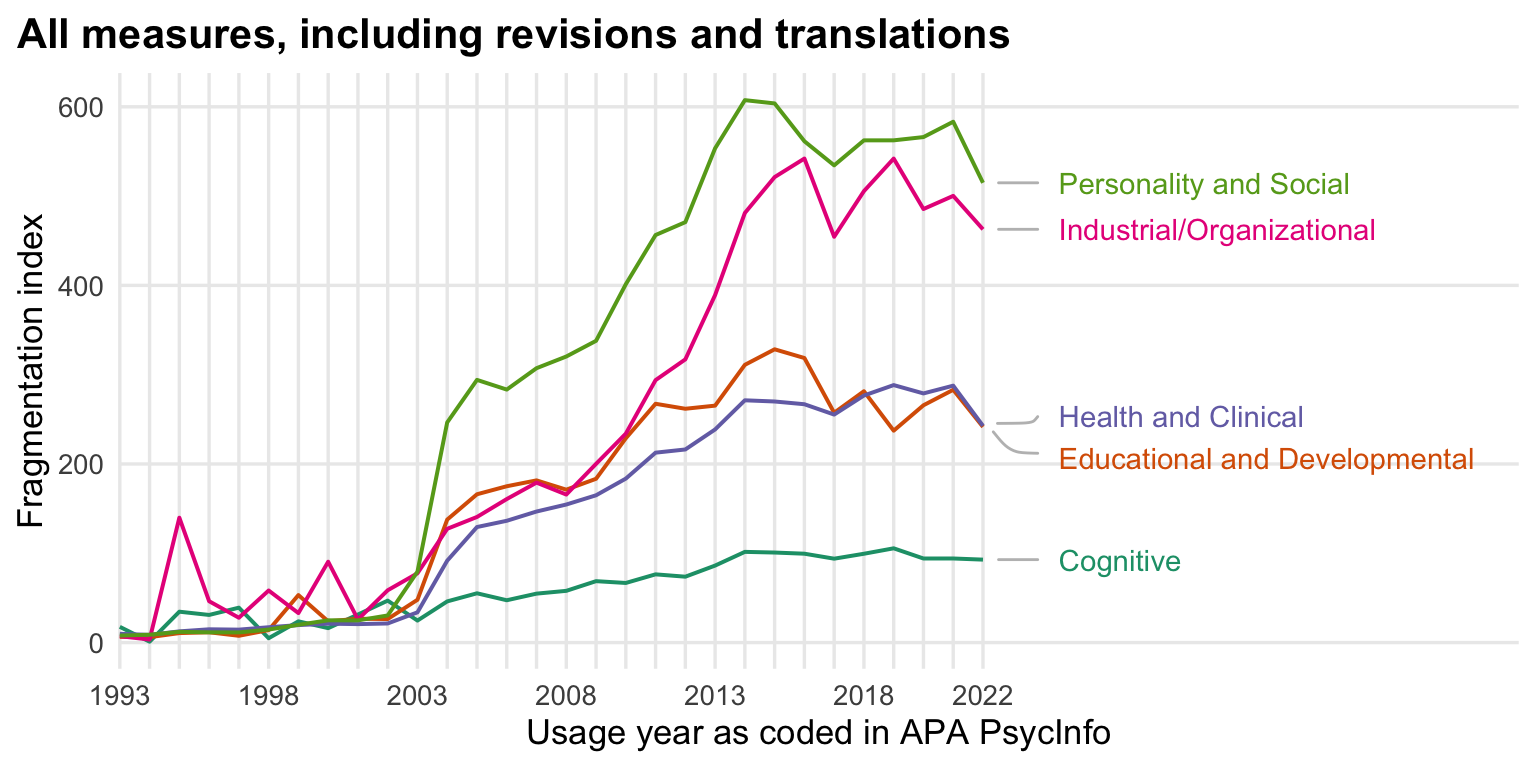
Show code
ggsave("figures/entropy_subdiscipline_constructs.pdf", width = 8, height = 4)
ggsave("figures/entropy_subdiscipline_constructs.png", width = 8, height = 4)
Rarefaction
Rarefaction involves resampling the tests in each year a number of times based off of the smallest sample-size (year with the smallest number of measure observations, 1993) to get a distribution of comparisons. This also allows us to get rid of the relativizing from zero to one, no matter what diversity measure we use.
Show code
# Set a seed for reproducibility
set.seed(05102019)

### 1. Define a simulation function for rarefaction

simulate_rarefaction <- function(freq, n_min, k = 50) {
  # freq: named numeric vector of counts (names are test IDs)
  # n_min: rarefaction depth (number of observations to sample)
  # k: number of resampling iterations
  res <- replicate(k, {
    # Expand the frequency vector into a vector of individual observations
    pop <- rep(names(freq), times = freq)
    # Sample without replacement the rarefaction depth number of individuals
    sample_ids <- sample(pop, size = n_min, replace = FALSE)
    tbl <- table(sample_ids)

    # Compute diversity metrics:
    richness     <- length(tbl)
    shannon      <- entropy(as.numeric(tbl))
    gini_simpson <- 1 - sum((as.numeric(tbl) / n_min)^2)
    hill_simpson <- hillR::hill_taxa(as.numeric(tbl), q = 2)
    hill_shannon <- hillR::hill_taxa(as.numeric(tbl), q = 1)
    # effective number of species (Hill number q=1)


    c(richness = richness,
      shannon = shannon,
      gini_simpson = gini_simpson,
      hill_simpson = hill_simpson,
      hill_shannon = hill_shannon)
  })

  # Convert the simulation output to a data frame:
  res_df <- as.data.frame(t(res))
  res_df$replicate <- 1:k
  res_df
}

### 2. Prepare counts for each grouping

# 2.1. All tests (using DOI as the test identifier)
counts_all <- psyctests_info %>%
  filter(between(Year, 1993, 2022)) %>%
  drop_na(DOI) %>%
  filter(usage_count > 0) %>%
  group_by(Year, Test = DOI) %>%
  summarise(n = sum(usage_count, na.rm = TRUE), .groups = "drop")

# 2.2. Revisions lumped (using if_else to recode tests)
counts_lumped <- psyctests_info %>%
  filter(between(Year, 1993, 2022)) %>%
  mutate(Test = if_else(test_type == "Original", DOI, original_test_DOI)) %>%
  drop_na(Test) %>%
  filter(usage_count > 0) %>%
  group_by(Year, Test) %>%
  summarise(n = sum(usage_count, na.rm = TRUE), .groups = "drop")


# 2.3. By construct (using first_construct as the test identifier)
counts_construct <- psyctests_info %>%
  filter(between(Year, 1993, 2022)) %>%
  filter(usage_count > 0) %>%
  drop_na(first_construct) %>%
  mutate(Test = first_construct) %>%
  group_by(Year, Test) %>%
  summarise(n = sum(usage_count, na.rm = TRUE), .groups = "drop")

### 3. A helper function to run rarefaction per count type

run_rarefaction <- function(counts_df, type_label, k = 500) {
  # Compute total counts per year for this type:
  yearly_totals <- counts_df %>%
    group_by(Year) %>%
    summarise(total = sum(n), .groups = "drop")

  # Set the rarefaction depth to the smallest total count across years:
  rarefaction_depth <- min(yearly_totals$total)

  # For each year, create the frequency vector and run the simulation:
  sim_data <- counts_df %>%
    group_by(Year) %>%
    summarise(freq = list(setNames(n, Test)), .groups = "drop") %>%
    left_join(yearly_totals, by = "Year") %>%
    mutate(sim = map(freq, ~ simulate_rarefaction(.x, n_min = rarefaction_depth, k = k))) %>%
    select(Year, sim) %>%
    unnest(sim) %>%
    mutate(type = type_label)

  sim_data
}

### 4. Run rarefaction for all three types

rare_all       <- run_rarefaction(counts_all,       "All tests")
rare_lumped    <- run_rarefaction(counts_lumped,    "Revisions lumped")
rare_construct <- run_rarefaction(counts_construct, "By construct")

# Combine the rarefaction results from all types:
rare_combined <- bind_rows(rare_all, rare_lumped, rare_construct)

# Pivot the data to long format for the metrics
rare_long <- rare_combined %>%
  pivot_longer(cols = c(richness, shannon, gini_simpson, hill_simpson, hill_shannon),
               names_to = "metric",
               values_to = "value")

# Summarize rarefaction results
rare_long <- rare_long %>%
  group_by(Year, type, metric) %>%
  summarise(
    mean = mean(value),
    lower = quantile(value, 0.025),
    upper = quantile(value, 0.975)
  )

rare_long <- rare_long %>%
  mutate(type = case_match(type,
                           "All tests" ~ "measures",
                           "By construct" ~ "constructs",
                            "Revisions lumped" ~ "with translations\n and revisions")) %>%
  mutate(metric = case_match(metric,
                             'hill_simpson' ~ "Hill-Simpson",
                             'hill_shannon' ~ "Hill-Shannon",
                             'richness' ~ "Species richness"))

### 5. Create a facet plot
# The facet grid is arranged with metrics in rows and count types in columns.
ggplot(rare_long %>% filter(metric %in% c("Hill-Simpson", "Hill-Shannon", "Species richness")), aes(x = Year, y = mean, min=lower, ymax = upper, color = type, fill = type)) +
  geom_smooth(stat = "identity") +
  # geom_line(stat = 'summary', fun = mean, color = "blue", size = 0.7, group = 1) +
  facet_grid(metric ~ ., scales = "free_y") +
  scale_color_brewer(type = "qual", guide = "none", palette = 2) +
  scale_fill_brewer(type = "qual", guide = "none", palette = 2) +
  theme_minimal(base_size = 14) +
  scale_color_brewer(type = "qual", guide = "none", palette = 2) +
  scale_x_continuous("Usage year as coded in APA PsycInfo", limits = c(1993, 2022),
                     breaks = seq(1993, 2022, by = 1),
                     labels = c(1993, "", "", "", "", 1998, "", "", "", "", 2003, "", "", "", "", 2008, "", "", "", "", 2013, "", "", "", "", 2018, "", "", "", "2022")) +
  labs(y = "Fragmentation index",
        title = "Standardized by Rarefaction")
Show code
ggsave("figures/diversity_indices_rarefaction.pdf", width = 8, height = 6)
ggsave("figures/diversity_indices_rarefaction.png", width = 8, height = 6)
Show code
rarefaction_hill_shannon <- rare_long %>% filter(metric %in% c( "Hill-Shannon"))

rarefaction_hill_shannon %>%
  ggplot(., aes(Year, y = mean, min=lower, ymax = upper, color = type, fill = type)) +
  geom_smooth(size = 0.7, stat = "identity") +
  scale_y_continuous("Fragmentation index") +
  scale_x_continuous("Usage year as coded in APA PsycInfo", limits = c(1993, 2030),
                     breaks = seq(1993, 2022, by = 1),
                     labels = c(1993, "", "", "", "", 1998, "", "", "", "", 2003, "", "", "", "", 2008, "", "", "", "", 2013, "", "", "", "", 2018, "", "", "", "2022")) +
  scale_color_brewer(type = "qual", guide = "none", palette = 2) +
  scale_fill_brewer(type = "qual", guide = "none", palette = 2) +
  geom_vline(xintercept = 2016, linetype = 'dashed') +
  geom_text_repel(data = rarefaction_hill_shannon %>% drop_na() %>% group_by(type) %>% filter(Year == max(Year, na.rm = T)),
                  aes(label = paste0(" ",type)), # "\n (n = ", n_tests, ")"
                  segment.curvature = -0.5,
                  segment.square = TRUE,
                  segment.color = 'grey',
                  xlim = c(2023, 2030),
                  nudge_x = 1.14,
                  lineheight = .9,
                  hjust = 0,
                  direction="y",
                  na.rm = TRUE) +
  theme_minimal(base_size = 13) +
   theme(
        panel.grid.minor.y = element_blank(),
        panel.grid.minor.x = element_blank(),
        plot.title.position = "plot",
        plot.title = element_text(face="bold"),
        legend.position = "none")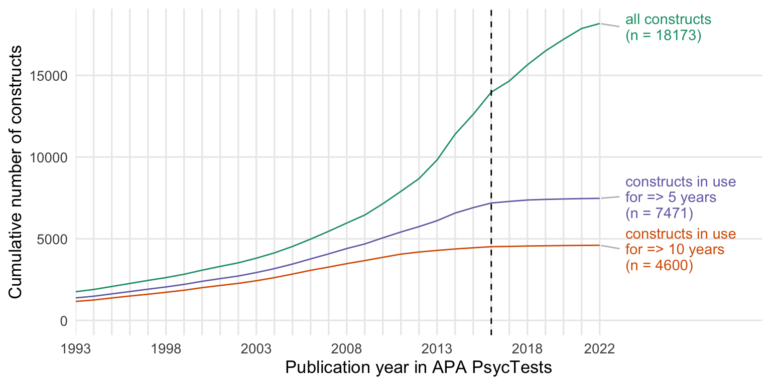
Show code
ggsave("figures/entropy_rarefaction.pdf", width = 8, height = 4)
ggsave("figures/entropy_rarefaction.png", width = 8, height = 4)
Rarefaction plus 25% chance of off by one
Primitive approach to check robustness of conclusions to off-by-one errors.
Show code
# Set a seed for reproducibility
set.seed(05102019)

### 1. Define a simulation function for rarefaction with per-sample error
simulate_rarefaction <- function(freq, pub_year, current_year, n_min, k = 50) {
  # freq: named numeric vector of counts (names are test IDs)
  # pub_year: named numeric vector of TestYear for each test (same names as freq)
  # current_year: the scalar year for this group
  # n_min: rarefaction depth (number of observations to sample)
  # k: number of resampling iterations
  res <- replicate(k, {
    # For each test, adjust the count with measurement error anew:
    freq_adj <- sapply(seq_along(freq), function(i) {
      if (is.na(pub_year[i]) || current_year < pub_year[i]) {
        # Before publication or missing publication info, force count to 0
        0
      } else {
        # With 25% chance, adjust the count by ±1; otherwise leave unchanged.
        adjustment <- if (runif(1) < 0.25) sample(c(-1, 1), size = 1) else 0
        new_val <- freq[i] + adjustment
        if (new_val < 0) 0 else new_val
      }
    })

    # Expand the adjusted frequency vector into individual observations
    pop <- rep(names(freq_adj), times = freq_adj)

    # If there are too few observations after error adjustment, return NA metrics.
    if (length(pop) < n_min) {
      return(c(richness = NA, shannon = NA, gini_simpson = NA, true_diversity = NA))
    }

    # Draw a rarefied sample without replacement.
    sample_ids <- sample(pop, size = n_min, replace = FALSE)
    tbl <- table(sample_ids)

    # Compute diversity metrics:
    richness     <- length(tbl)
    shannon      <- entropy(as.numeric(tbl))
    gini_simpson <- 1 - sum((as.numeric(tbl) / n_min)^2)
    true_diversity <- exp(shannon)  # effective number of species (Hill number q=1)

    c(richness = richness,
      shannon = shannon,
      gini_simpson = gini_simpson,
      true_diversity = true_diversity)
  })

  # Convert the simulation output to a data frame.
  res_df <- as.data.frame(t(res))
  res_df$replicate <- 1:k
  res_df
}

### 2. Prepare counts for each grouping (bringing along TestYear)

# 2.1. All tests (using DOI as the test identifier)
counts_all <- psyctests_info %>%
  filter(between(Year, 1993, 2022)) %>%
  drop_na(DOI) %>%
  filter(usage_count > 0) %>%
  group_by(Year, Test = DOI) %>%
  summarise(n = sum(usage_count, na.rm = TRUE),
            TestYear = min(TestYear),
            .groups = "drop")

# 2.2. Revisions lumped (using if_else to recode tests)
counts_lumped <- psyctests_info %>%
  filter(between(Year, 1993, 2022)) %>%
  mutate(Test = if_else(test_type == "Original", DOI, original_test_DOI)) %>%
  drop_na(Test) %>%
  filter(usage_count > 0) %>%
  group_by(Year, Test) %>%
  summarise(n = sum(usage_count, na.rm = TRUE),
            TestYear = min(TestYear),
            .groups = "drop")

# 2.3. By construct (using first_construct as the test identifier)
counts_construct <- psyctests_info %>%
  filter(between(Year, 1993, 2022)) %>%
  filter(usage_count > 0) %>%
  drop_na(first_construct) %>%
  mutate(Test = first_construct) %>%
  group_by(Year, Test) %>%
  summarise(n = sum(usage_count, na.rm = TRUE),
            TestYear = min(TestYear),
            .groups = "drop")

### 3. A helper function to run rarefaction per count type with per-sample error
run_rarefaction <- function(counts_df, type_label, k = 500) {
  # Compute total counts per year for this type:
  yearly_totals <- counts_df %>%
    group_by(Year) %>%
    summarise(total = sum(n), .groups = "drop")

  # Set the rarefaction depth to the smallest total count across years:
  rarefaction_depth <- min(yearly_totals$total)

  # For each year, create the frequency vector and the publication year vector,
  # then run the simulation using pmap so that the scalar Year is passed along.
  sim_data <- counts_df %>%
    group_by(Year) %>%
    summarise(
      freq = list(setNames(n, Test)),
      pub  = list(setNames(TestYear, Test)),
      .groups = "drop"
    ) %>%
    left_join(yearly_totals, by = "Year") %>%
    mutate(sim = pmap(
      list(freq, pub, Year),
      function(freq, pub, Year) {
        simulate_rarefaction(
          freq = freq,
          pub_year = pub,
          current_year = Year,
          n_min = rarefaction_depth,
          k = k
        )
      }
    )) %>%
    select(Year, sim) %>%
    unnest(sim) %>%
    mutate(type = type_label)

  sim_data
}

### 4. Run rarefaction for all three types
rare_all       <- run_rarefaction(counts_all,       "All tests")
rare_lumped    <- run_rarefaction(counts_lumped,    "Revisions lumped")
rare_construct <- run_rarefaction(counts_construct, "By construct")

# Combine the rarefaction results from all types:
rare_combined <- bind_rows(rare_all, rare_lumped, rare_construct)


# Pivot the data to long format for the metrics
rare_long <- rare_combined %>%
  pivot_longer(cols = c(richness, shannon, gini_simpson, true_diversity),
               names_to = "metric",
               values_to = "value")

# Summarize rarefaction results (mean and 95% intervals)
rare_long <- rare_long %>%
  group_by(Year, type, metric) %>%
  summarise(
    mean = mean(value, na.rm = TRUE),
    lower = quantile(value, 0.025, na.rm = TRUE),
    upper = quantile(value, 0.975, na.rm = TRUE)
  )


rare_long <- rare_long %>%
  mutate(type = case_match(type,
                           "All tests" ~ "measures",
                           "By construct" ~ "constructs",
                            "Revisions lumped" ~ "with translations\n and revisions")) %>%
  mutate(metric = case_match(metric,
                             'hill_simpson' ~ "Hill-Simpson",
                             'hill_shannon' ~ "Hill-Shannon",
                             'richness' ~ "Species richness"))

### 5. Create a facet plot
# The facet grid is arranged with metrics in rows and count types in columns.
ggplot(rare_long %>% filter(metric %in% c("Hill-Simpson", "Hill-Shannon", "Species richness")), aes(x = Year, y = mean, min=lower, ymax = upper, color = type, fill = type)) +
  geom_smooth(stat = "identity") +
  # geom_line(stat = 'summary', fun = mean, color = "blue", size = 0.7, group = 1) +
  facet_grid(metric ~ ., scales = "free_y") +
  scale_color_brewer(type = "qual", guide = "none", palette = 2) +
  scale_fill_brewer(type = "qual", guide = "none", palette = 2) +
  theme_minimal(base_size = 14) +
  scale_color_brewer(type = "qual", guide = "none", palette = 2) +
  scale_x_continuous("Usage year as coded in APA PsycInfo", limits = c(1993, 2022),
                     breaks = seq(1993, 2022, by = 1),
                     labels = c(1993, "", "", "", "", 1998, "", "", "", "", 2003, "", "", "", "", 2008, "", "", "", "", 2013, "", "", "", "", 2018, "", "", "", "2022")) +
  labs(y = "Fragmentation index",
        title = "Standardized by Rarefaction + 25% off-by-one errors",
        subtitle = "For published tests, counts are adjusted by ±1 with 25% probability anew per simulation")
Show code
ggsave("figures/diversity_indices_rarefaction_ob1.pdf", width = 8, height = 6)
ggsave("figures/diversity_indices_rarefaction_ob1.png", width = 8, height = 6)
Old approach: Normalised Shannon Entropy
Show code
byorig_entropy_by_year <- psyctests_info %>%
  filter(between(Year, 1993, 2022)) %>%
  mutate(Test = if_else(test_type == "Original", DOI, original_test_DOI)) %>%
  drop_na(Test) %>%
  group_by(Year, Test) %>%
  summarise(n = sum(usage_count, na.rm = T)) %>%
  ungroup() %>%
  mutate(n_tests = n_distinct(Test)) %>%
  group_by(n_tests, Year) %>%
  filter(n > 0) %>%
  summarise(entropy = entropy(n),
            norm_entropy = calc_norm_entropy(n),
            n = sum(n),
            diff_tests = n()) %>%
  ungroup()
# what's the point of mutate(n_tests = n_distinct(Test))? just to check?


byconstruct_entropy_by_year <- psyctests_info %>%
  filter(between(Year, 1993, 2022)) %>%
  drop_na(first_construct) %>%
  group_by(Year, Test = first_construct) %>%
  summarise(n = sum(usage_count, na.rm = T)) %>%
  ungroup() %>%
  mutate(n_tests = n_distinct(Test)) %>%
  group_by(n_tests, Year) %>%
  filter(n > 0) %>%
  summarise(entropy = entropy(n),,
            norm_entropy = calc_norm_entropy(n),
            n = sum(n),
            diff_tests = n()) %>%
  ungroup()

all_entropy_by_year <- psyctests_info %>%
  filter(between(Year, 1993, 2022)) %>%
  drop_na(DOI) %>%
  group_by(Year, Test = DOI) %>%
  summarise(n = sum(usage_count, na.rm = T)) %>%
  ungroup() %>%
  mutate(n_tests = n_distinct(Test)) %>%
  group_by(n_tests, Year) %>%
  filter(n > 0) %>%
  summarise(entropy = entropy(n),,
            norm_entropy = calc_norm_entropy(n),
            n = sum(n),
            diff_tests = n()) %>%
  ungroup()

original_entropy_by_year <- psyctests_info %>%
  filter(between(Year, 1993, 2022)) %>%
  filter(test_type == "Original") %>%
  group_by(Year, Test = DOI) %>%
  summarise(n = sum(usage_count, na.rm = T)) %>%
  ungroup() %>%
  mutate(n_tests = n_distinct(Test)) %>%
  group_by(n_tests, Year) %>%
  filter(n > 0) %>%
  summarise(entropy = entropy(n),,
            norm_entropy = calc_norm_entropy(n),
            n = sum(n),
            diff_tests = n()) %>%
  ungroup()

entropy_by_year <- bind_rows(# "all tests" = all_entropy_by_year,
                             "measures" = original_entropy_by_year,
                             "with translations\n and revisions" = byorig_entropy_by_year,
                             # "by name base" = bybase_entropy_by_year,
                             "constructs" = byconstruct_entropy_by_year,
                             .id = "version")


entropy_by_year %>%
  ggplot(., aes(Year, norm_entropy, color = version)) +
  geom_line(size = 0.7) +
  scale_y_continuous("Normalized Shannon Entropy", limits = c(0, 1), labels = scales::percent) +
  # geom_line(aes(y = log(n)), color = 'red') +
  scale_x_continuous("Usage year as coded in APA PsycInfo", limits = c(1993, 2030),
                     breaks = seq(1993, 2022, by = 1),
                     labels = c(1993, "", "", "", "", 1998, "", "", "", "", 2003, "", "", "", "", 2008, "", "", "", "", 2013, "", "", "", "", 2018, "", "", "", "2022")) +
  scale_color_brewer(type = "qual", guide = "none", palette = 2) +
  geom_vline(xintercept = 2016, linetype = 'dashed') +
  # ggrepel::geom_text_repel(
  #   aes(label = str_replace(subdiscipline, " Psychology", "")), data = entropy_by_year %>% filter(Year == max(Year, na.rm = T)),
  #   size = 4, hjust = 1,
  #   ) +
  geom_text_repel(data = entropy_by_year %>% drop_na() %>% group_by(version) %>% filter(Year == max(Year, na.rm = T)),
                  aes(label = paste0(" ",version)), # "\n (n = ", n_tests, ")"
                  segment.curvature = -0.5,
                  segment.square = TRUE,
                  segment.color = 'grey',
                  xlim = c(2023, 2030),
                  nudge_x = 1.14,
                  lineheight = .9,
                  hjust = 0,
                  direction="y",
                  na.rm = TRUE) +
  theme_minimal(base_size = 13) +
   theme(
        panel.grid.minor.y = element_blank(),
        panel.grid.minor.x = element_blank(),
        plot.title.position = "plot",
        plot.title = element_text(face="bold"),
        legend.position = "none")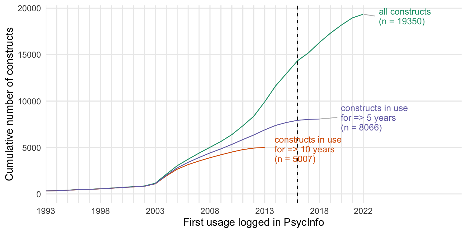
by subdiscipline
all measures
Show code
entropy_by_year <- psyctests_info %>%
  filter(between(Year, 1993, 2022)) %>%
  group_by(subdiscipline_1, Year, Test = DOI) %>%
  summarise(n = sum(usage_count, na.rm = T)) %>%
  group_by(subdiscipline_1) %>%
  mutate(n_tests = n_distinct(Test)) %>%
  group_by(subdiscipline_1, n_tests, Year) %>%
  filter(n > 0) %>%
  summarise(entropy = entropy(n),,
            norm_entropy = calc_norm_entropy(n),
            n = sum(n),
            diff_tests = n()) %>%
  ungroup()


entropy_by_year %>%
  ggplot(., aes(Year, norm_entropy, color = subdiscipline_1)) +
  geom_line(size = 0.7) +
  scale_y_continuous("Normalized Shannon Entropy\n(with revisions and translations)", limits = c(0, 1), labels = scales::percent) +
  # geom_line(aes(y = log(n)), color = 'red') +
  scale_x_continuous("Usage year as coded in APA PsycInfo", limits = c(1993, 2033),
                     breaks = seq(1993,2022, by = 1),
                     labels = c(1993, "", "", "", "", 1998, "", "", "", "", 2003, "", "", "", "", 2008, "", "", "", "", 2013, "", "", "", "", 2018, "", "", "", "2022"),
                     expand = expansion(add = c(0, 14))) +
  scale_color_brewer(type = "qual", guide = "none", palette = 2) +
  # ggtitle(str_c(n_distinct(tests_by_year$Test), " measures tracked in PsycInfo")) +
 # geom_text_repel(aes(label = gsub("^.*$", " ", subdiscipline_1)), # This will force the correct position of the link's right end.
 #                  data = entropy_by_year %>% drop_na() %>% group_by(subdiscipline_1) %>% filter(Year == max(Year, na.rm = T)),
 #                  segment.curvature = -0.1,
 #                  segment.square = TRUE,
 #                  segment.color = 'grey',
 #                  box.padding = 0.1,
 #                  point.padding = 0.6,
 #                  max.overlaps = Inf,
 #                  nudge_x = 1.3,
 #                  # nudge_y = 0,
 #                  force = 20,
 #                  hjust = 0,
 #                  direction="y",
 #                  na.rm = TRUE
 #  ) +
  geom_text_repel(data = entropy_by_year %>% drop_na() %>% group_by(subdiscipline_1) %>% filter(Year == max(Year, na.rm = T)),
                  aes(label = paste0("  ",str_replace(subdiscipline_1, " Psychology", ""), " (n=", n_tests, ")")),
                  # segment.alpha = 0, ## This will 'hide' the link
                  segment.curvature = -0.1,
                  segment.square = TRUE,
                  segment.color = 'grey',
                  box.padding = 0.1,
                  max.overlaps = Inf,
                  point.padding = 0.6,
                  xlim = c(2022, NA),
                  nudge_x = 2,
                  # nudge_y = 0.0,
                  force = 5,
                  hjust = 0,
                  direction="y",
                  na.rm = F) +
  theme_minimal(base_size = 13) +
   theme(panel.grid.minor.y = element_blank(),
        panel.grid.minor.x = element_blank(),
        plot.title.position = "plot",
        plot.title = element_text(face="bold"),
        legend.position = "none") +
    coord_cartesian(clip = "off")
original measures
Show code
entropy_by_year <- psyctests_info %>%
  filter(between(Year, 1993, 2022)) %>%
  mutate(Test = if_else(test_type == "Original", DOI, original_test_DOI)) %>%
  drop_na(Test) %>%
  group_by(subdiscipline_1, Year, Test) %>%
  summarise(n = sum(usage_count, na.rm = T)) %>%
  group_by(subdiscipline_1) %>%
  mutate(n_tests = n_distinct(Test)) %>%
  group_by(subdiscipline_1, n_tests, Year) %>%
  filter(n > 0) %>%
  summarise(entropy = entropy(n),,
            norm_entropy = calc_norm_entropy(n),
            n = sum(n),
            diff_tests = n()) %>%
  ungroup()


entropy_by_year %>%
  ggplot(., aes(Year, norm_entropy, color = subdiscipline_1)) +
  geom_line(size = 0.7) +
  scale_y_continuous("Normalized Shannon Entropy\n(novel measures)", limits = c(0, 1), labels = scales::percent) +
  # geom_line(aes(y = log(n)), color = 'red') +
  scale_x_continuous("Usage year as coded in APA PsycInfo", limits = c(1993, 2030),
                     breaks = seq(1993, 2022, by = 1),
                     labels = c(1993, "", "", "", "", 1998, "", "", "", "", 2003, "", "", "", "", 2008, "", "", "", "", 2013, "", "", "", "", 2018, "", "", "", "2022"),
                     expand = expansion(add = c(0, 17))) +
  scale_color_brewer(type = "qual", guide = "none", palette = 2) +
  # ggtitle(str_c(n_distinct(tests_by_year$Test), " measures tracked in PsycInfo")) +
 # geom_text_repel(aes(label = gsub("^.*$", " ", subdiscipline_1)), # This will force the correct position of the link's right end.
 #                  data = entropy_by_year %>% drop_na() %>% group_by(subdiscipline_1) %>% filter(Year == max(Year, na.rm = T)),
 #                  segment.curvature = -0.1,
 #                  segment.square = TRUE,
 #                  segment.color = 'grey',
 #                  box.padding = 0.1,
 #                  point.padding = 0.6,
 #                  max.overlaps = Inf,
 #                  nudge_x = 1.3,
 #                  # nudge_y = 0,
 #                  force = 20,
 #                  hjust = 0,
 #                  direction="y",
 #                  na.rm = TRUE
 #  ) +
  geom_text_repel(data = entropy_by_year %>% drop_na() %>% group_by(subdiscipline_1) %>% filter(Year == max(Year, na.rm = T)),
                  aes(label = paste0("  ",str_replace(subdiscipline_1, " Psychology", ""), " (n=", n_tests, ")")),
                  # segment.alpha = 0, ## This will 'hide' the link
                  segment.curvature = -0.1,
                  segment.square = TRUE,
                  segment.color = 'grey',
                  box.padding = 0.1,
                  max.overlaps = Inf,
                  point.padding = 0.6,
                  xlim = c(2022, NA),
                  nudge_x = 2,
                  # nudge_y = 0.0,
                  force = 5,
                  hjust = 0,
                  direction="y",
                  na.rm = F)  +
   theme(panel.grid.minor.y = element_blank(),
        panel.grid.minor.x = element_blank(),
        plot.title.position = "plot",
        plot.title = element_text(face="bold"),
        legend.position = "none") +
    coord_cartesian(clip = "off")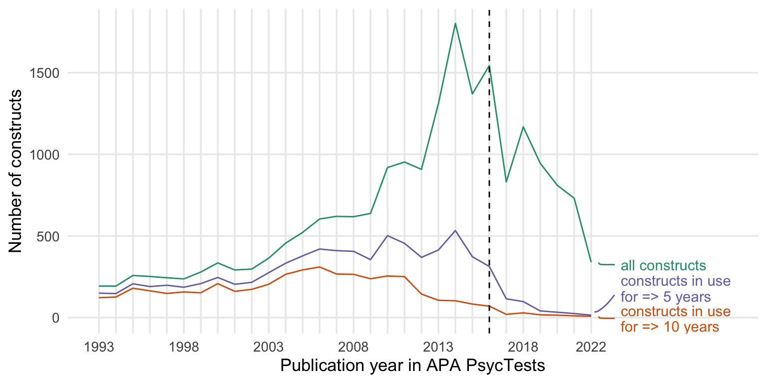
constructs
Show code
entropy_by_year <- psyctests_info %>%
  filter(between(Year, 1993, 2022)) %>%
  group_by(subdiscipline_1, Year, Test = first_construct) %>%
  summarise(n = sum(usage_count, na.rm = T)) %>%
  group_by(subdiscipline_1) %>%
  mutate(n_tests = n_distinct(Test)) %>%
  group_by(subdiscipline_1, n_tests, Year) %>%
  filter(n > 0) %>%
  summarise(entropy = entropy(n),,
            norm_entropy = calc_norm_entropy(n),
            n = sum(n),
            diff_tests = n()) %>%
  ungroup()


entropy_by_year %>%
  ggplot(., aes(Year, norm_entropy, color = subdiscipline_1)) +
  geom_line(size = 0.7) +
  scale_y_continuous("Normalized Shannon Entropy (constructs)", limits = c(0, 1), labels = scales::percent) +
  # geom_line(aes(y = log(n)), color = 'red') +
  scale_x_continuous("Usage year as coded in APA PsycInfo", limits = c(1993, 2038),
                     breaks = seq(1993, 2022, by = 1),
                     labels = c(1993, "", "", "", "", 1998, "", "", "", "", 2003, "", "", "", "", 2008, "", "", "", "", 2013, "", "", "", "", 2018, "", "", "", "2022"),
                     expand = expansion(add = c(0, 10))) +
  scale_color_brewer(type = "qual", guide = "none", palette = 2) +
  # ggtitle(str_c(n_distinct(tests_by_year$Test), " measures tracked in PsycInfo")) +
  # ggrepel::geom_text_repel(
  #   aes(label = str_replace(subdiscipline, " Psychology", "")), data = entropy_by_year %>% filter(Year == max(Year, na.rm = T)),
  #   size = 4, hjust = 1,
  #   ) +
  geom_text_repel(data = entropy_by_year %>% drop_na() %>% group_by(subdiscipline_1) %>% filter(Year == max(Year, na.rm = T)),
                  aes(label = paste0("  ",str_replace(subdiscipline_1, " Psychology", ""), " (n=", n_tests, ")")),
                  # segment.alpha = 0, ## This will 'hide' the link
                  segment.curvature = -0.1,
                  segment.square = TRUE,
                  segment.color = 'grey',
                  box.padding = 0.1,
                  max.overlaps = Inf,
                  point.padding = 0.6,
                  xlim = c(2022, NA),
                  nudge_x = 2,
                  # nudge_y = 0.0,
                  force = 5,
                  hjust = 0,
                  direction="y",
                  na.rm = F) +
   theme(panel.grid.minor.y = element_blank(),
        panel.grid.minor.x = element_blank(),
        plot.title.position = "plot",
        plot.title = element_text(face="bold"),
        legend.position = "none")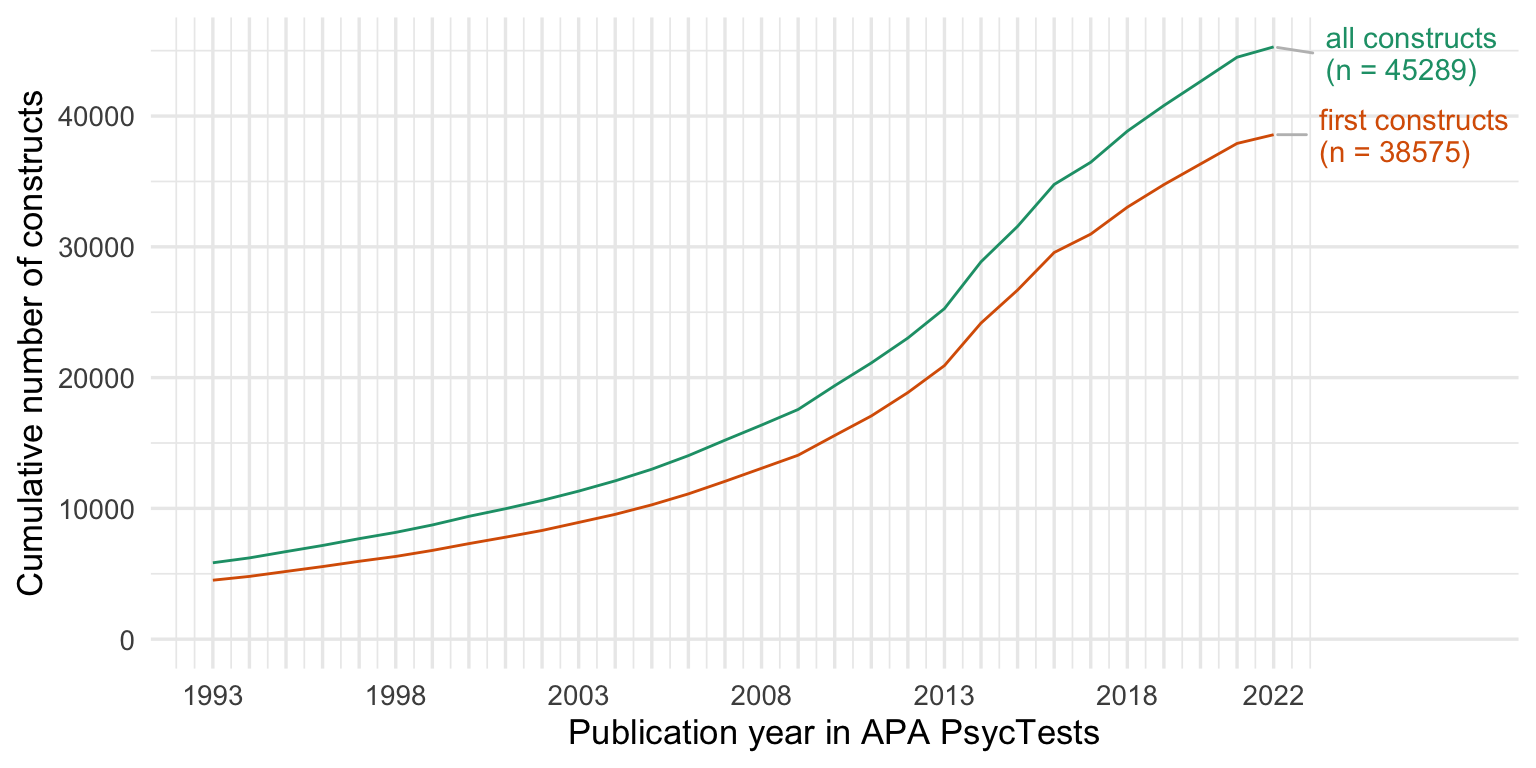
By instrument type
Show code
entropy_by_year <- psyctests_info %>%
  filter(between(Year, 1993, 2022)) %>%
  group_by(instrument_type_broad, Year, Test = DOI) %>%
  summarise(n = sum(usage_count, na.rm = T)) %>%
  group_by(instrument_type_broad) %>%
  mutate(n_tests = n_distinct(Test)) %>%
  group_by(instrument_type_broad, n_tests, Year) %>%
  filter(n > 0) %>%
  summarise(entropy = entropy(n),
            norm_entropy = calc_norm_entropy(n),
            n = sum(n),
            diff_tests = n()) %>%
  ungroup()


entropy_by_year %>%
  ggplot(., aes(Year, norm_entropy, color = instrument_type_broad)) +
  geom_line(size = 0.7) +
  scale_y_continuous("Normalized Shannon Entropy", limits = c(0, 1), labels = scales::percent) +
  # geom_line(aes(y = log(n)), color = 'red') +
  scale_x_continuous(limits = c(1993, 2027), breaks = c(1993, 1998, 2003, 2008, 2013, 2018, 2022)) +
  scale_color_brewer(type = "qual", guide = "none", palette = 3) +
  # ggrepel::geom_text_repel(
  #   aes(label = str_replace(subdiscipline, " Psychology", "")), data = entropy_by_year %>% filter(Year == max(Year, na.rm = T)),
  #   size = 4, hjust = 1,
  #   ) +
  geom_text_repel(aes(label = gsub("^.*$", " ", instrument_type_broad)), # This will force the correct position of the link's right end.
                  data = entropy_by_year %>% filter(Year == max(Year, na.rm = T)),
                  segment.curvature = -0.1,
                  segment.square = TRUE,
                  segment.color = 'grey',
                  box.padding = 0.1,
                  point.padding = 0.6,
                  nudge_x = 0.15,
                  nudge_y = 0.05,
                  force = 0.5,
                  hjust = 0,
                  direction="y",
                  na.rm = TRUE
  ) +
  geom_text_repel(data = entropy_by_year %>% filter(Year == max(Year, na.rm = T)),
                  aes(label = paste0("  ",str_replace(instrument_type_broad, " Psychology", ""), " (n=", n_tests, ")")),
                  segment.alpha = 0, ## This will 'hide' the link
                  segment.curvature = -0.1,
                  segment.square = TRUE,
                  # segment.color = 'grey',
                  box.padding = 0.1,
                  point.padding = 0.6,
                  nudge_x = 0.15,
                  nudge_y = 0.05,
                  force = 0.5,
                  hjust = 0,
                  direction="y",
                  na.rm = TRUE)+
  theme_minimal(base_size = 13) +
   theme(panel.grid.minor.y = element_blank(),
        panel.grid.minor.x = element_blank(),
        plot.title.position = "plot",
        plot.title = element_text(face="bold"),
        legend.position = "none")
Lorenz curves
Show code
test_frequency <- psyctests_info %>%
  mutate(Test = if_else(test_type == "Original", DOI, original_test_DOI)) %>%
  drop_na(Test) %>%
  # filter(TestYear >= 1990) %>%
  filter(between(Year, 1993, 2022)) %>%
  group_by(subdiscipline_1, Test) %>%
  summarise(n = sum(usage_count, na.rm = T)) %>%
  arrange(n) %>%
  mutate(decile = Hmisc::cut2(n, g = 10)) %>%
  mutate(cumsum = cumsum(n),
         sum = sum(n))
#
# test_frequency %>%
#     group_by(subdiscipline_1, decile) %>%
#     summarise(share = sum(n)/first(sum),
#               median_n = median(n),
#               n_measures = n()) %>%
#   View()


ggplot(test_frequency, aes(n)) +
  stat_lorenz(desc = F) +
  coord_fixed() +
  geom_abline(linetype = "dashed") +
      theme_minimal() +
    hrbrthemes::scale_x_percent("Cumulative percentage of measures") +
    hrbrthemes::scale_y_percent("Cumulative percentage of measure market share") #+
Show code
#    hrbrthemes::theme_ipsum_rc()

ggplot(test_frequency, aes(n, color = subdiscipline_1)) +
  stat_lorenz(desc = F) +
  coord_fixed() +
  geom_abline(linetype = "dashed") +
      theme_minimal() +
    hrbrthemes::scale_x_percent("Cumulative percentage of measures") +
    hrbrthemes::scale_y_percent("Cumulative percentage of measure market share")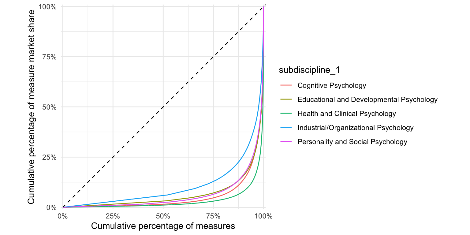
Survival
aggregate stats
Show code
constructs <- psyctests_info %>%
     # filter(between(first_pub_year, 1950, 2015)) %>%
     unnest(ConstructList) %>%
     rowwise() %>%
     mutate(construct = unlist(ConstructList)) %>%
     select(-ConstructList) %>%
     filter(between(Year, 1993, 2022)) %>%
     drop_na(construct) %>%
     mutate(survival = last_pub_year - first_pub_year,
            survived_five = if_else(survival >= 5, T, F),
            survived_ten = if_else(survival >= 10, T, F)) %>%
     distinct(construct, .keep_all = TRUE)

mean(constructs$survival, na.rm = T)
[1] 6.120457Show code
sd(constructs$survival, na.rm = T)[1] 8.788988Show code
median(constructs$survival, na.rm = T)[1] 2Show code
max(constructs$survival, na.rm = T)[1] 122Show code
min(constructs$survival, na.rm = T)[1] 0Show code
[1] 6.046785Show code
sd(measures$survival, na.rm = T)[1] 8.743927Show code
median(measures$survival, na.rm = T)[1] 2Show code
max(measures$survival, na.rm = T)[1] 122Show code
min(measures$survival, na.rm = T)[1] 0cumulative sum
all constructs
Show code
cumsum_construct <- constructs %>%
  arrange(TestYear) %>%
  group_by(TestYear) %>%
  summarise(constructs = n_distinct(DOI)) %>%
  arrange(TestYear) %>%
  mutate(constructs = cumsum(constructs))

cumsum_construct_survived_5 <- constructs %>%
  filter(survived_five == T) %>%
  arrange(TestYear) %>%
  group_by(TestYear) %>%
  summarise(constructs = n_distinct(DOI)) %>%
  arrange(TestYear) %>%
  mutate(constructs = cumsum(constructs))

cumsum_construct_survived_10 <- constructs %>%
  filter(survived_ten == T) %>%
  arrange(TestYear) %>%
  group_by(TestYear) %>%
  summarise(constructs = n_distinct(DOI)) %>%
  arrange(TestYear) %>%
  mutate(constructs = cumsum(constructs))


cumsums <- bind_rows(
  "all constructs" = cumsum_construct,
  "constructs in use\n for => 5 years" = cumsum_construct_survived_5,
  "constructs in use\n for => 10 years" = cumsum_construct_survived_10,
  .id = "origin"
  ) %>%
  rename(Year = TestYear) %>%
  filter(Year <= 2022)


ggplot(cumsums, aes(Year, constructs, color = origin)) +
  geom_line() +
  geom_vline(xintercept = 2016, linetype = 'dashed') +
  scale_y_continuous("Cumulative number of constructs") +
  scale_x_continuous("Publication year in APA PsycTests",
                     limits = c(1993, 2030),
                     breaks = seq(1993,2022, by = 1),
                     labels = c(1993, "", "", "", "", 1998, "", "", "", "", 2003, "", "", "", "", 2008, "", "", "", "", 2013, "", "", "", "", 2018, "", "", "", "2022"),
                     expand = expansion(add = c(0, 1))) +
  scale_color_brewer(type = "qual", guide = "none", palette = 2) +
  # ggrepel::geom_text_repel(
  #   aes(label = str_replace(subdiscipline, " Psychology", "")), data = entropy_by_year %>% filter(Year == max(Year, na.rm = T)),
  #   size = 4, hjust = 1,
  #   )  +
  geom_text_repel(data = cumsums %>% drop_na() %>% group_by(origin) %>% filter(Year == max(Year, na.rm = T)),
                  aes(label = paste0(" ", origin, "\n (n = ", constructs, ")")),
                  segment.square = TRUE,
                  lineheight = .9,
                  segment.color = 'grey',
                  nudge_x = 1.2,
                  hjust = 0,
                  na.rm = TRUE)+
   # theme_minimal(base_size = 13) +
   theme(panel.grid.minor.y = element_blank(),
        panel.grid.minor.x = element_blank(),
        plot.title.position = "plot",
        plot.title = element_text(face="bold"),
        legend.position = "none")  +
    guides(
    x = guide_axis(cap = "both"), # Cap both ends
  )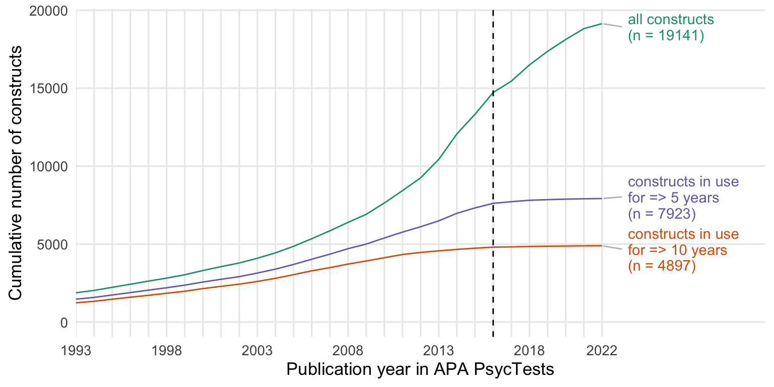
Show code
ggsave("figures/cumsums_survival_all.pdf", width = 8, height = 4)
ggsave("figures/cumsums_survival_all.png", width = 8, height = 4)
first constructs
Show code
first_constructs <- constructs %>%
  distinct(first_construct, .keep_all = TRUE)


cumsum_construct <- first_constructs %>%
  arrange(TestYear) %>%
  group_by(TestYear) %>%
  summarise(constructs = n_distinct(DOI)) %>%
  arrange(TestYear) %>%
  mutate(constructs = cumsum(constructs))

cumsum_construct_survived_5 <- first_constructs %>%
  filter(survived_five == T) %>%
  arrange(TestYear) %>%
  group_by(TestYear) %>%
  summarise(constructs = n_distinct(DOI)) %>%
  arrange(TestYear) %>%
  mutate(constructs = cumsum(constructs))

cumsum_construct_survived_10 <- first_constructs %>%
  filter(survived_ten == T) %>%
  arrange(TestYear) %>%
  group_by(TestYear) %>%
  summarise(constructs = n_distinct(DOI)) %>%
  arrange(TestYear) %>%
  mutate(constructs = cumsum(constructs))


cumsums <- bind_rows(
  "all constructs" = cumsum_construct,
  "constructs in use\n for => 5 years" = cumsum_construct_survived_5,
  "constructs in use\n for => 10 years" = cumsum_construct_survived_10,
  .id = "origin"
  ) %>%
  rename(Year = TestYear) %>%
  filter(Year <= 2022)


ggplot(cumsums, aes(Year, constructs, color = origin)) +
  geom_line() +
  geom_vline(xintercept = 2016, linetype = 'dashed') +
  scale_y_continuous("Cumulative number of constructs") +
  scale_x_continuous("Publication year in APA PsycTests",
                     limits = c(1993, 2030),
                     breaks = seq(1993,2022, by = 1),
                     labels = c(1993, "", "", "", "", 1998, "", "", "", "", 2003, "", "", "", "", 2008, "", "", "", "", 2013, "", "", "", "", 2018, "", "", "", "2022"),
                     expand = expansion(add = c(0, 1))) +
  scale_color_brewer(type = "qual", guide = "none", palette = 2) +
  # ggrepel::geom_text_repel(
  #   aes(label = str_replace(subdiscipline, " Psychology", "")), data = entropy_by_year %>% filter(Year == max(Year, na.rm = T)),
  #   size = 4, hjust = 1,
  #   )  +
  geom_text_repel(data = cumsums %>% drop_na() %>% group_by(origin) %>% filter(Year == max(Year, na.rm = T)),
                  aes(label = paste0(" ", origin, "\n (n = ", constructs, ")")),
                  segment.square = TRUE,
                  lineheight = .9,
                  segment.color = 'grey',
                  nudge_x = 1.2,
                  hjust = 0,
                  na.rm = TRUE)+
   # theme_minimal(base_size = 13) +
   theme(panel.grid.minor.y = element_blank(),
        panel.grid.minor.x = element_blank(),
        plot.title.position = "plot",
        plot.title = element_text(face="bold"),
        legend.position = "none")  +
    guides(
    x = guide_axis(cap = "both"), # Cap both ends
  )
Show code
ggsave("figures/cumsums_survival_first.pdf", width = 8, height = 4)
ggsave("figures/cumsums_survival_first.png", width = 8, height = 4)
measures
Show code
cumsum_all <- measures %>%
  group_by(TestYear) %>%
  summarise(tests = n()) %>%
  arrange(TestYear) %>%
  mutate(tests = cumsum(tests))

cumsum_5 <- measures %>%
  filter(survived_five == T) %>%
  group_by(TestYear) %>%
  summarise(tests = n()) %>%
  arrange(TestYear) %>%
  mutate(tests = cumsum(tests))

cumsum_10 <- measures %>%
  filter(survived_ten == T) %>%
  arrange(TestYear) %>%
  distinct(Name_base, .keep_all = T) %>%
  group_by(TestYear) %>%
  summarise(tests = n_distinct(DOI)) %>%
  mutate(tests = cumsum(tests))

cumsums <- bind_rows(
  "all measures" = cumsum_all,
  "measures in use\n for => 5 years" = cumsum_5,
  "measures in use\n for => 10 years" = cumsum_10,
  .id = "origin"
  ) %>%
  rename(Year = TestYear) %>%
  filter(Year <= 2022)


ggplot(cumsums, aes(Year, tests, color = origin)) +
  geom_line() +
  geom_vline(xintercept = 2016, linetype = 'dashed') +
  scale_y_continuous("Cumulative number of measures") +
  scale_x_continuous("Publication year in APA PsycTests",
                     limits = c(1993, 2030),
                     breaks = seq(1993,2022, by = 1),
                     labels = c(1993, "", "", "", "", 1998, "", "", "", "", 2003, "", "", "", "", 2008, "", "", "", "", 2013, "", "", "", "", 2018, "", "", "", "2022"),
                     expand = expansion(add = c(0, 1))) +
  scale_color_brewer(type = "qual", guide = "none", palette = 2) +
  # ggrepel::geom_text_repel(
  #   aes(label = str_replace(subdiscipline, " Psychology", "")), data = entropy_by_year %>% filter(Year == max(Year, na.rm = T)),
  #   size = 4, hjust = 1,
  #   )  +
  geom_text_repel(data = cumsums %>% drop_na() %>% group_by(origin) %>% filter(Year == max(Year, na.rm = T)),
                  aes(label = paste0(" ", origin, "\n (n = ", tests, ")")),
                  segment.square = TRUE,
                  lineheight = .9,
                  segment.color = 'grey',
                  nudge_x = 1.2,
                  hjust = 0,
                  na.rm = TRUE) +
   # theme_minimal(base_size = 13) +
   theme(panel.grid.minor.y = element_blank(),
        panel.grid.minor.x = element_blank(),
        plot.title.position = "plot",
        plot.title = element_text(face="bold"),
        legend.position = "none")  +
    guides(
    x = guide_axis(cap = "both"), # Cap both ends
  )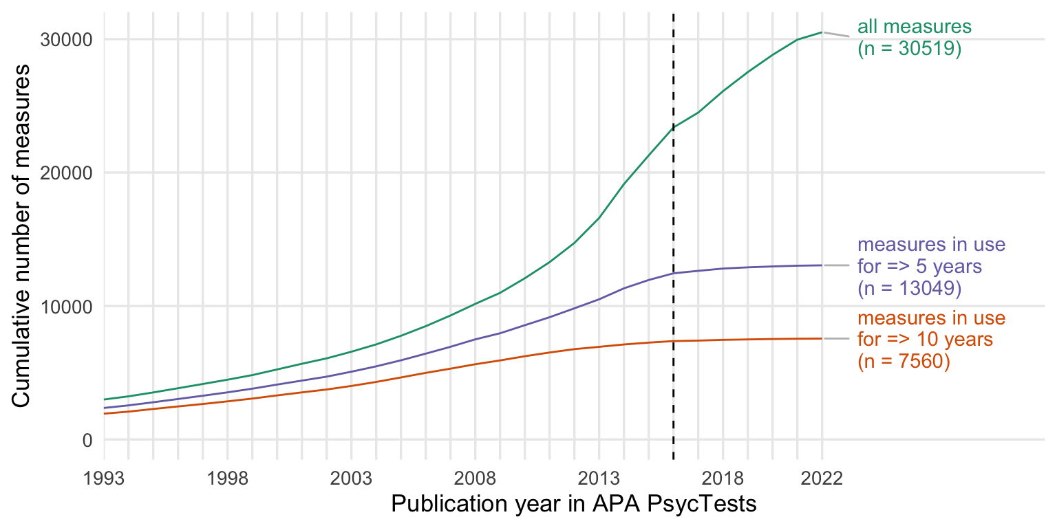
Show code
ggsave("figures/cumsums_survival_measures.pdf", width = 8, height = 4)
ggsave("figures/cumsums_survival_measures.png", width = 8, height = 4)
by first use in PsycInfo instead of publication year in PsycTests
Show code
cumsum_construct <- constructs %>%
  arrange(first_pub_year) %>%
  group_by(first_pub_year) %>%
  summarise(constructs = n_distinct(DOI)) %>%
  arrange(first_pub_year) %>%
  mutate(constructs = cumsum(constructs))

cumsum_construct_survived_5 <- constructs %>%
  filter(survived_five == T) %>%
  arrange(first_pub_year) %>%
  group_by(first_pub_year) %>%
  summarise(constructs = n_distinct(DOI)) %>%
  arrange(first_pub_year) %>%
  mutate(constructs = cumsum(constructs))

cumsum_construct_survived_10 <- constructs %>%
  filter(survived_ten == T) %>%
  arrange(first_pub_year) %>%
  group_by(first_pub_year) %>%
  summarise(constructs = n_distinct(DOI)) %>%
  arrange(first_pub_year) %>%
  mutate(constructs = cumsum(constructs))


cumsums <- bind_rows(
  "all constructs" = cumsum_construct,
  "constructs in use\n for => 5 years" = cumsum_construct_survived_5,
  "constructs in use\n for => 10 years" = cumsum_construct_survived_10,
  .id = "origin"
  ) %>%
  rename(Year = first_pub_year) %>%
  filter(Year <= 2022)


ggplot(cumsums, aes(Year, constructs, color = origin)) +
  geom_line() +
  geom_vline(xintercept = 2016, linetype = 'dashed') +
  scale_y_continuous("Cumulative number of constructs") +
  scale_x_continuous("First usage logged in PsycInfo",
                     limits = c(1993, 2030),
                     breaks = seq(1993,2022, by = 1),
                     labels = c(1993, "", "", "", "", 1998, "", "", "", "", 2003, "", "", "", "", 2008, "", "", "", "", 2013, "", "", "", "", 2018, "", "", "", "2022"),
                     expand = expansion(add = c(0, 1))) +
  scale_color_brewer(type = "qual", guide = "none", palette = 2) +
  # ggrepel::geom_text_repel(
  #   aes(label = str_replace(subdiscipline, " Psychology", "")), data = entropy_by_year %>% filter(Year == max(Year, na.rm = T)),
  #   size = 4, hjust = 1,
  #   )  +
  geom_text_repel(data = cumsums %>% drop_na() %>% group_by(origin) %>% filter(Year == max(Year, na.rm = T)),
                  aes(label = paste0(" ", origin, "\n (n = ", constructs, ")")),
                  segment.square = TRUE,
                  lineheight = .9,
                  segment.color = 'grey',
                  nudge_x = 1.2,
                  hjust = 0,
                  na.rm = TRUE)+
   # theme_minimal(base_size = 13) +
   theme(panel.grid.minor.y = element_blank(),
        panel.grid.minor.x = element_blank(),
        plot.title.position = "plot",
        plot.title = element_text(face="bold"),
        legend.position = "none")  +
    guides(
    x = guide_axis(cap = "both"), # Cap both ends
  )
by last use in PsycInfo instead of publication year in PsycTests
Show code
cumsum_construct <- constructs %>%
  arrange(last_pub_year) %>%
  group_by(last_pub_year) %>%
  summarise(constructs = n_distinct(DOI)) %>%
  arrange(last_pub_year) %>%
  mutate(constructs = cumsum(constructs))

cumsum_construct_survived_5 <- constructs %>%
  filter(survived_five == T) %>%
  arrange(last_pub_year) %>%
  group_by(last_pub_year) %>%
  summarise(constructs = n_distinct(DOI)) %>%
  arrange(last_pub_year) %>%
  mutate(constructs = cumsum(constructs))

cumsum_construct_survived_10 <- constructs %>%
  filter(survived_ten == T) %>%
  arrange(last_pub_year) %>%
  group_by(last_pub_year) %>%
  summarise(constructs = n_distinct(DOI)) %>%
  arrange(last_pub_year) %>%
  mutate(constructs = cumsum(constructs))


cumsums <- bind_rows(
  "all constructs" = cumsum_construct,
  "constructs in use\n for => 5 years" = cumsum_construct_survived_5,
  "constructs in use\n for => 10 years" = cumsum_construct_survived_10,
  .id = "origin"
  ) %>%
  rename(Year = last_pub_year) %>%
  filter(Year <= 2022)


ggplot(cumsums, aes(Year, constructs, color = origin)) +
  geom_line() +
  geom_vline(xintercept = 2016, linetype = 'dashed') +
  scale_y_continuous("Cumulative number of constructs") +
  scale_x_continuous("Last usage logged in PsycInfo",
                     limits = c(1993, 2030),
                     breaks = seq(1993,2022, by = 1),
                     labels = c(1993, "", "", "", "", 1998, "", "", "", "", 2003, "", "", "", "", 2008, "", "", "", "", 2013, "", "", "", "", 2018, "", "", "", "2022"),
                     expand = expansion(add = c(0, 1))) +
  scale_color_brewer(type = "qual", guide = "none", palette = 2) +
  # ggrepel::geom_text_repel(
  #   aes(label = str_replace(subdiscipline, " Psychology", "")), data = entropy_by_year %>% filter(Year == max(Year, na.rm = T)),
  #   size = 4, hjust = 1,
  #   )  +
  geom_text_repel(data = cumsums %>% drop_na() %>% group_by(origin) %>% filter(Year == max(Year, na.rm = T)),
                  aes(label = paste0(" ", origin, "\n (n = ", constructs, ")")),
                  segment.square = TRUE,
                  lineheight = .9,
                  segment.color = 'grey',
                  nudge_x = 1.2,
                  hjust = 0,
                  na.rm = TRUE)+
   # theme_minimal(base_size = 13) +
   theme(panel.grid.minor.y = element_blank(),
        panel.grid.minor.x = element_blank(),
        plot.title.position = "plot",
        plot.title = element_text(face="bold"),
        legend.position = "none")  +
    guides(
    x = guide_axis(cap = "both"), # Cap both ends
  )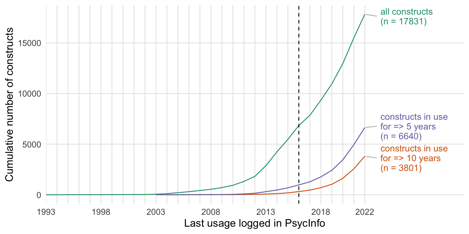
counts
Show code
count_construct <- constructs %>%
  arrange(TestYear) %>%
  group_by(TestYear) %>%
  summarise(tests = n_distinct(construct)) %>%
  arrange(TestYear)

count_construct_5 <- constructs %>%
  filter(survived_five == T) %>%
  arrange(TestYear) %>%
  group_by(TestYear) %>%
  summarise(tests = n_distinct(construct)) %>%
  arrange(TestYear)

count_construct_10 <- constructs %>%
  filter(survived_ten == T) %>%
  arrange(TestYear) %>%
  group_by(TestYear) %>%
  summarise(tests = n_distinct(construct)) %>%
  arrange(TestYear)

counts <- bind_rows(
  "all constructs" = count_construct,
  "constructs in use\n for => 5 years" = count_construct_5,
  "constructs in use\n for => 10 years" = count_construct_10,
  .id = "origin"
  ) %>%
  rename(Year = TestYear) %>%
  filter(Year <= 2022)


ggplot(counts, aes(Year, tests, color = origin)) +
  geom_line() +
  geom_vline(xintercept = 2016, linetype = 'dashed') +
  scale_y_continuous("Number of constructs") +
  scale_x_continuous("Publication year in APA PsycTests",
                     limits = c(1993, 2030),
                     breaks = seq(1993, 2022, by = 1),
                     labels = c(1993, "", "", "", "", 1998, "", "", "", "", 2003, "", "", "", "", 2008, "", "", "", "", 2013, "", "", "", "", 2018, "", "", "", "2022")) +
  scale_color_brewer(type = "qual", guide = "none", palette = 2) +
  # ggrepel::geom_text_repel(
  #   aes(label = str_replace(subdiscipline, " Psychology", "")), data = entropy_by_year %>% filter(Year == max(Year, na.rm = T)),
  #   size = 4, hjust = 1,
  #   ) +
  geom_text_repel(data = counts %>% drop_na() %>% group_by(origin) %>% filter(Year == max(Year, na.rm = T)),
                  aes(label = paste0(" ", origin)),
                  segment.curvature = -0.1,
                  segment.square = TRUE,
                  lineheight = .9,
                  # segment.color = 'grey',
                  box.padding = 0.1,
                  point.padding = 0.6,
                  nudge_x = 1.5,
                  nudge_y = -15,
                  force = 1,
                  hjust = 0,
                  direction="y",
                  na.rm = F) +
   theme(panel.grid.minor.y = element_blank(),
        panel.grid.minor.x = element_blank(),
        plot.title.position = "plot",
        plot.title = element_text(face="bold"),
        legend.position = "none")
Show code
ggsave("figures/counts_survival.pdf", width = 8, height = 4)
ggsave("figures/counts_survival.png", width = 8, height = 4)
Robustness checks
Show code
all_constructs_over_time <- records_wide %>% select(subdiscipline_1, DOI, TestYear, ConstructList) %>%
    unnest(ConstructList) %>%
    rowwise() %>%
    mutate(construct = unlist(ConstructList)) %>%
  select(-ConstructList)

cumsum_all_constructs <- all_constructs_over_time %>%
  arrange(TestYear) %>%
  distinct(construct, .keep_all = T) %>%
  group_by(TestYear) %>%
  summarise(constructs = n_distinct(construct)) %>%
  arrange(TestYear) %>%
  mutate(constructs = cumsum(constructs))


cumsum_construct <- records_wide %>%
  arrange(TestYear) %>%
  distinct(first_construct, .keep_all = T) %>%
  group_by(TestYear) %>%
  summarise(constructs = n_distinct(first_construct)) %>%
  arrange(TestYear) %>%
  mutate(constructs = cumsum(constructs))

cumsums <- bind_rows(
  "first constructs" = cumsum_construct,
  "all constructs" = cumsum_all_constructs,
  .id = "origin"
  ) %>%
  rename(Year = TestYear) %>%
  filter(Year <= 2022)


ggplot(cumsums, aes(Year, constructs, color = origin)) +
  geom_line() +
  scale_y_continuous("Cumulative number of constructs") +
  scale_x_continuous("Publication year in APA PsycTests",
                     limits = c(1993, 2027),
                     breaks = seq(1993, 2022, by = 1),
                     labels = c(1993, "", "", "", "", 1998, "", "", "", "", 2003, "", "", "", "", 2008, "", "", "", "", 2013, "", "", "", "", 2018, "", "", "", "2022")) +
  scale_color_brewer(type = "qual", guide = "none", palette = 2) +
  # ggrepel::geom_text_repel(
  #   aes(label = str_replace(subdiscipline, " Psychology", "")), data = entropy_by_year %>% filter(Year == max(Year, na.rm = T)),
  #   size = 4, hjust = 1,
  #   ) +
  geom_text_repel(data = cumsums %>% drop_na() %>% group_by(origin) %>% filter(Year == max(Year, na.rm = T)),
                  aes(label = paste0(" ", origin, "\n (n = ", constructs, ")")),
                  segment.square = TRUE,
                  lineheight = .9,
                  segment.color = 'grey',
                  nudge_x = 1.2,
                  hjust = 0,
                  na.rm = TRUE)
Show code
ggsave("figures/cumsum_all_vs_first.pdf", width = 8, height = 4)
ggsave("figures/cumsum_all_vs_first.png", width = 8, height = 4)
All or first constructs
For some 20% of tests, two or more constructs were coded. In most plots, we simply use the first construct for each test.
Show code
    1     2     3     4     5     6     7     8     9    10    12
56645 12421  2134   326    85    37    13    14     3     3     3
   15    16    17    21    22    23    25
    1     1     1     1     1     1     2
Show code
round(prop.table(table(records_wide$constructs_n)),2)
   1    2    3    4    5    6    7    8    9   10   12   15   16   17
0.79 0.17 0.03 0.00 0.00 0.00 0.00 0.00 0.00 0.00 0.00 0.00 0.00 0.00
  21   22   23   25
0.00 0.00 0.00 0.00
Show code
ggplot(records_wide, aes(constructs_n)) +
  geom_bar()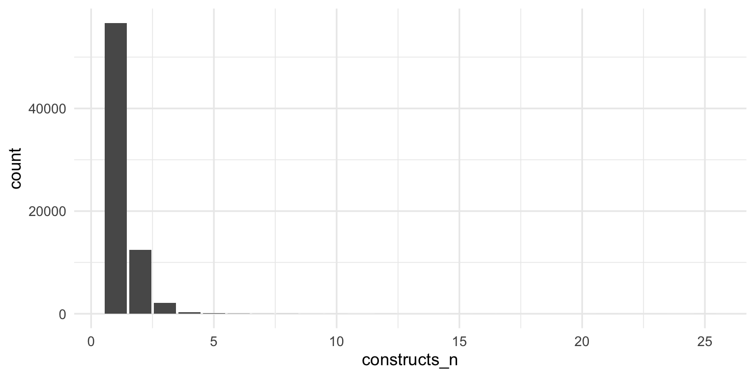
Expanding the entropy calculation to all coded constructs makes little difference.
Show code
all_constructs_over_time <- psyctests_info %>% select(subdiscipline_1, DOI, TestYear, Year, ConstructList, usage_count) %>%
    unnest(ConstructList) %>%
    rowwise() %>%
    mutate(construct = unlist(ConstructList)) %>%
  select(-ConstructList)

entropy_all_constructs <- all_constructs_over_time %>%
  filter(between(Year, 1993, 2022)) %>%
  drop_na(construct) %>%
  group_by(Year, construct) %>%
  summarise(n = sum(usage_count, na.rm = T)) %>%
  ungroup() %>%
  mutate(n_tests = n_distinct(construct)) %>%
  group_by(n_tests, Year) %>%
  filter(n > 0) %>%
  summarise(
    tests = list(as.numeric(n)),
    entropy = entropy(n),,
            norm_entropy = calc_norm_entropy(n),
        hill_shannon = hillR::hill_taxa(n, q = 1),

            n = sum(n),
            diff_tests = n()) %>%
  ungroup()

byconstruct_entropy_by_year <- psyctests_info %>%
  filter(between(Year, 1993, 2022)) %>%
  drop_na(first_construct) %>%
  group_by(Year, Test = first_construct) %>%
  summarise(n = sum(usage_count, na.rm = T)) %>%
  ungroup() %>%
  mutate(n_tests = n_distinct(Test)) %>%
  group_by(n_tests, Year) %>%
  filter(n > 0) %>%
  summarise(
    tests = list(as.numeric(n)),
    total_n = sum(n),
    entropy = entropy(n),,
    norm_entropy = calc_norm_entropy(n),
    hill_shannon = hillR::hill_taxa(n, q = 1),
    n = sum(n),
    diff_tests = n()) %>%
  ungroup()

entropy_by_year <- bind_rows(# "all tests" = all_entropy_by_year,
                             "all constructs" = entropy_all_constructs,
                             # "by name base" = bybase_entropy_by_year,
                             "first constructs" = byconstruct_entropy_by_year,
                             .id = "version")

entropy_by_year %>%
  ggplot(., aes(Year, hill_shannon, color = version)) +
  geom_line(size = 0.7) +
  scale_y_continuous("Hill-Shannon Diversity") +
  # geom_line(aes(y = log(n)), color = 'red') +
  scale_x_continuous("Usage year as coded in APA PsycInfo", limits = c(1993, 2027),
                     breaks = seq(1993, 2022, by = 1),
                     labels = c(1993, "", "", "", "", 1998, "", "", "", "", 2003, "", "", "", "", 2008, "", "", "", "", 2013, "", "", "", "", 2018, "", "", "", "2022")) +

  scale_color_brewer(type = "qual", guide = "none", palette = 2) +
  # ggrepel::geom_text_repel(
  #   aes(label = str_replace(subdiscipline, " Psychology", "")), data = entropy_by_year %>% filter(Year == max(Year, na.rm = T)),
  #   size = 4, hjust = 1,
  #   ) +
  geom_text_repel(data = entropy_by_year %>% group_by(version) %>% filter(Year == max(Year, na.rm = T)),
                  aes(label = paste0(" ",version)), # "\n (n = ", n_tests, ")"
                  segment.curvature = -0.5,
                  segment.square = TRUE,
                  segment.color = 'grey',
                  xlim = c(2023, 2030),
                  nudge_x = 1.14,
                  lineheight = .9,
                  hjust = 0,
                  direction="y",
                  na.rm = TRUE) +
  theme_minimal(base_size = 13) +
   theme(panel.grid.minor.y = element_blank(),
        panel.grid.minor.x = element_blank(),
        plot.title.position = "plot",
        plot.title = element_text(face="bold"),
        legend.position = "none")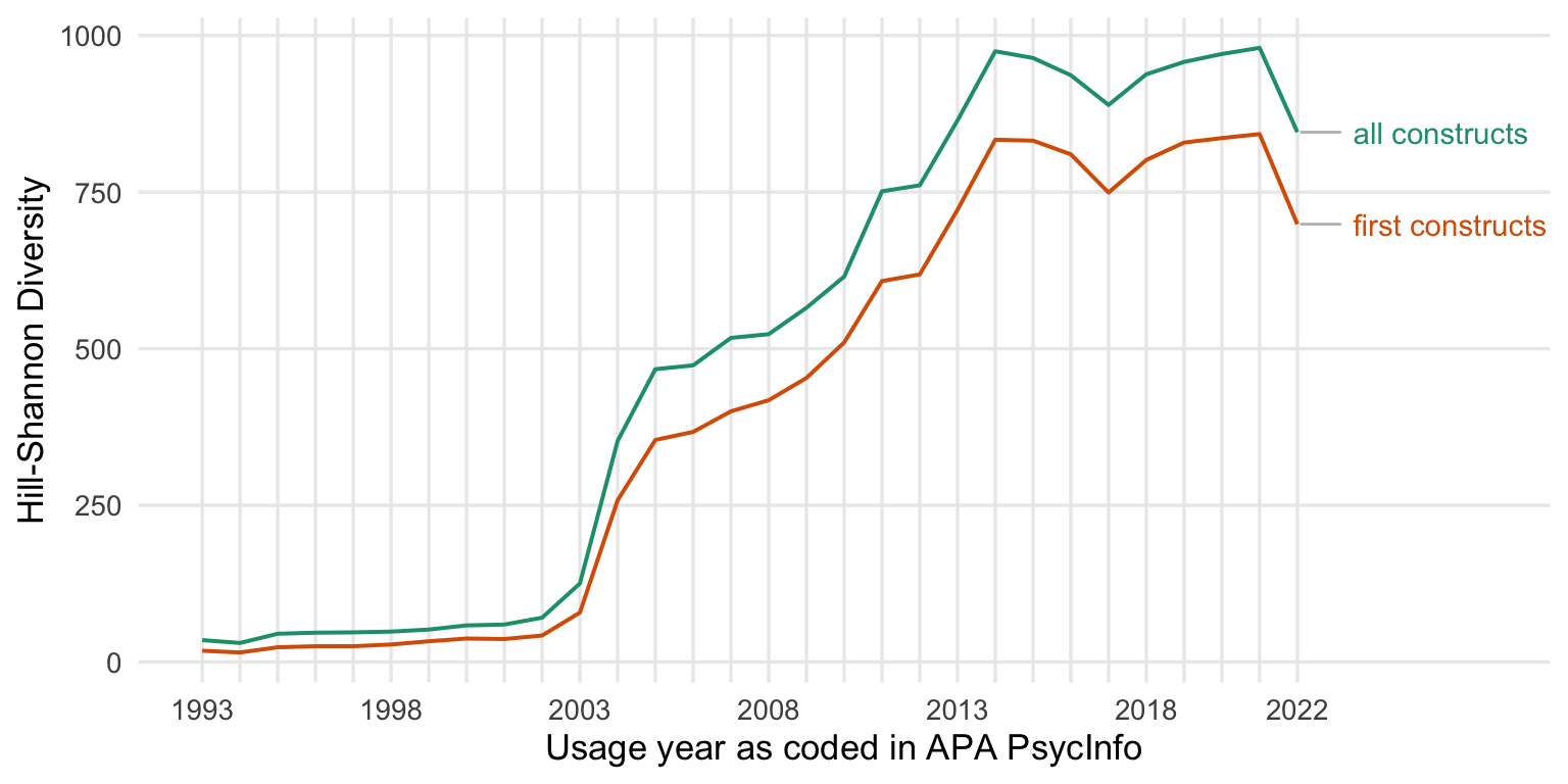
Show code
ggsave("figures/entropy_all_vs_first.pdf", width = 8, height = 4)
ggsave("figures/entropy_all_vs_first.png", width = 8, height = 4)
Entropy by classification
Show code
entropy_by_class <- psyctests_info %>%
  filter(between(Year, 1993, 2022)) %>%
  mutate(Test = if_else(test_type == "Original", DOI, original_test_DOI)) %>%
  group_by(classification_1, Test) %>%
  summarise(n = sum(usage_count, na.rm = T)) %>%
  group_by(classification_1) %>%
  # filter(n > 0) %>%
  summarise(
    tbl = list(as.numeric(n)),
    total_n = sum(n),
    entropy = entropy(n),
    norm_entropy = calc_norm_entropy(n),
    hill_shannon = hillR::hill_taxa(n, q = 1)) %>%
  arrange(norm_entropy)

entropy_by_class_list <- entropy_by_class %>% select(classification_1, tbl) %>%
  deframe()
Show code
entropy_by_class_inext <- iNEXT(entropy_by_class_list) # , endpoint = 1000, knots = 10
ggiNEXT(entropy_by_class_inext, color.var = 'None')
Error in `palette()`:
! Insufficient values in manual scale. 31 needed but only 8
provided.Show code
entropy_by_class <- entropy_by_class %>% select(-tbl) %>% full_join(
  entropy_by_class_inext$AsyEst %>% rename(classification_1 = Assemblage) %>%
    mutate(diversity_estimate = sprintf("%.0f [%.0f;%.0f]", Estimator, LCL, UCL)) %>%
    # mutate(diversity_estimate = Estimator) %>%
    select(classification_1, diversity_estimate, Diversity) %>%
    pivot_wider(values_from = diversity_estimate, names_from = Diversity)
)

kable(entropy_by_class %>% arrange(`Shannon diversity` %>% str_extract("([0-9]+) ") %>% as.numeric(), hill_shannon))| classification_1 | total_n | entropy | norm_entropy | hill_shannon | Species richness | Shannon diversity | Simpson diversity |
|---|---|---|---|---|---|---|---|
| Intelligence | 7284 | 1.936077 | 0.5490299 | 6.931508 | 44 [34;80] | 7 [7;7] | 5 [5;5] |
| Military Personnel, Adjustment, and Training | 4453 | 1.969452 | 0.4206315 | 7.166747 | 169 [129;210] | 7 [7;8] | 4 [4;4] |
| Aptitude and Achievement | 4326 | 1.996436 | 0.4782585 | 7.362771 | 80 [65;104] | 7 [7;8] | 5 [4;5] |
| General Assessment Tools | 1403 | 2.209249 | 0.4999613 | 9.108874 | 121 [88;154] | 10 [9;11] | 4 [3;4] |
| Anxiety and Depression | 46429 | 2.992137 | 0.4813136 | 19.928224 | 701 [638;764] | 20 [20;20] | 8 [8;8] |
| Neuropsychological Assessment | 40220 | 3.084879 | 0.5202518 | 21.864832 | 541 [471;611] | 22 [22;22] | 10 [10;11] |
| Functional Status and Adaptive Behavior | 13507 | 3.284067 | 0.5645529 | 26.684077 | 655 [541;768] | 27 [26;28] | 12 [11;12] |
| Legal and Forensic Evaluation | 4529 | 3.449960 | 0.6070047 | 31.499119 | 480 [405;555] | 33 [31;35] | 9 [8;10] |
| Perceptual, Motor, and Sensory Processing | 5738 | 3.520288 | 0.6515822 | 33.794166 | 410 [327;494] | 35 [34;36] | 14 [13;15] |
| Emotional States, Emotional Responses, and Motivation | 38778 | 3.544672 | 0.5337411 | 34.628321 | 1167 [1066;1268] | 35 [34;36] | 10 [10;10] |
| Addiction, Gambling, and Substance Abuse/Use | 36817 | 3.573186 | 0.5433288 | 35.629915 | 1132 [1040;1224] | 36 [35;37] | 10 [10;10] |
| Sports, Recreation, and Leisure | 4825 | 3.611987 | 0.6296420 | 37.039577 | 518 [448;589] | 39 [37;42] | 9 [9;10] |
| Religious and Political Beliefs | 4132 | 3.652164 | 0.6311091 | 38.558002 | 514 [447;581] | 41 [39;44] | 10 [10;11] |
| Culture, Racial, and Ethnic Identity | 6153 | 3.726453 | 0.6439467 | 41.531547 | 436 [385;487] | 43 [41;45] | 13 [12;14] |
| Communication, Language, and Verbal Processing | 2790 | 3.694919 | 0.6789113 | 40.242318 | 465 [377;553] | 44 [40;47] | 13 [12;14] |
| Trauma, Stress, and Coping | 38159 | 3.848689 | 0.5720890 | 46.931513 | 1394 [1258;1530] | 48 [47;49] | 17 [16;17] |
| Cognitive Processes, Memory, and Decision Making | 49219 | 3.858750 | 0.5818379 | 47.406069 | 1112 [1031;1192] | 48 [47;49] | 16 [16;16] |
| Development and Aging | 36420 | 4.178621 | 0.6023399 | 65.275788 | 1862 [1704;2021] | 67 [65;68] | 14 [13;14] |
| Sex, Gender Roles, and Sexual Behavior | 10381 | 4.241755 | 0.6697565 | 69.529799 | 807 [729;885] | 73 [70;76] | 20 [19;20] |
| Mental Health/Illness Related Assessment | 255535 | 4.352307 | 0.5817821 | 77.657418 | 2700 [2549;2850] | 78 [77;79] | 28 [28;28] |
| Human Factors and Environmental Engineering | 1044 | 4.145539 | 0.7699030 | 63.151640 | 638 [506;770] | 83 [73;93] | 26 [22;30] |
| Consumer Behavior, Marketing, and Advertising | 2415 | 4.350168 | 0.7401094 | 77.491464 | 1044 [833;1256] | 93 [87;100] | 28 [25;30] |
| Attitudes, Interests, Values, and Expectancies | 13711 | 4.475760 | 0.6580759 | 87.861379 | 1484 [1358;1611] | 93 [90;96] | 24 [23;25] |
| Human-Computer Interaction | 2081 | 4.432384 | 0.7509163 | 84.131733 | 656 [560;751] | 100 [92;107] | 21 [19;23] |
| Personality | 71623 | 4.599470 | 0.6361150 | 99.431584 | 1977 [1866;2088] | 101 [99;103] | 23 [23;24] |
| Family Relationships and Parenting | 20446 | 4.626174 | 0.6696103 | 102.122556 | 1813 [1649;1978] | 107 [104;110] | 27 [26;28] |
| Treatment, Rehabilitation, and Therapeutic Processes | 30240 | 4.657907 | 0.6011396 | 105.415164 | 4826 [4546;5106] | 114 [110;118] | 12 [12;13] |
| Social, Group, and Interpersonal Relationships | 27392 | 4.852731 | 0.6805980 | 128.089695 | 2099 [1949;2249] | 133 [130;137] | 33 [32;34] |
| Organizational, Occupational, and Career Development | 21713 | 4.942498 | 0.6661604 | 140.119799 | 3098 [2848;3347] | 151 [146;156] | 19 [18;20] |
| Physical Health/Illness Related Assessment | 45177 | 5.011744 | 0.6626486 | 150.166406 | 3299 [3120;3478] | 156 [153;159] | 32 [31;33] |
| Education, Teaching, and Student Characteristics | 17691 | 4.951154 | 0.6480872 | 141.338031 | 4537 [4241;4834] | 161 [154;168] | 12 [11;12] |
Entropy by instrument type
Show code
entropy_by_instrument <- psyctests_info %>%
  filter(between(Year, 1993, 2022)) %>%
  mutate(Test = if_else(test_type == "Original", DOI, original_test_DOI)) %>%
  group_by(instrument_type_broad, Test) %>%
  summarise(n = sum(usage_count, na.rm = T)) %>%
  group_by(instrument_type_broad) %>%
  filter(n > 0) %>%
  summarise(
    tbl = list(as.numeric(n)),
    total_n = sum(n),
    entropy = entropy(n),
    norm_entropy = calc_norm_entropy(n),
    hill_shannon = hillR::hill_taxa(n, q = 1)) %>%
  arrange(hill_shannon)


entropy_by_instrument_list <- entropy_by_instrument %>% select(instrument_type_broad, tbl) %>%
  deframe()
entropy_by_instrument_inext <- iNEXT(entropy_by_instrument_list, endpoint = 1000, knots = 10)
ggiNEXT(entropy_by_instrument_inext)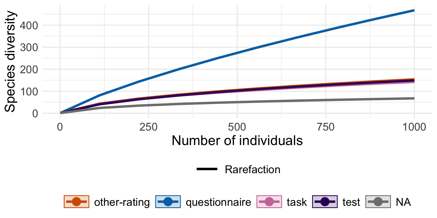
Show code
entropy_by_instrument <- entropy_by_instrument %>% select(-tbl) %>% full_join(
  entropy_by_instrument_inext$AsyEst %>% rename(instrument_type_broad = Assemblage) %>%
    mutate(diversity_estimate = sprintf("%.0f [%.0f;%.0f]", Estimator, LCL, UCL)) %>%
    # mutate(diversity_estimate = Estimator) %>%
    select(instrument_type_broad, diversity_estimate, Diversity) %>%
    pivot_wider(values_from = diversity_estimate, names_from = Diversity)
)
entropy_by_instrument %>%
kable()| instrument_type_broad | total_n | entropy | norm_entropy | hill_shannon | Species richness | Shannon diversity | Simpson diversity |
|---|---|---|---|---|---|---|---|
| NA | 12993 | 2.549405 | 0.4904120 | 12.79949 | 285 [227;343] | 13 [13;13] | 6 [6;6] |
| test | 80256 | 3.576240 | 0.5167475 | 35.73890 | 1669 [1536;1802] | 36 [36;37] | 10 [10;10] |
| task | 23705 | 3.763432 | 0.5971220 | 43.09610 | 852 [759;946] | 44 [43;45] | 16 [16;16] |
| other-rating | 61962 | 3.908466 | 0.5656449 | 49.82249 | 1702 [1555;1849] | 51 [50;51] | 19 [18;19] |
| questionnaire | 685715 | 6.380357 | 0.6462648 | 590.13864 | 33802 [33153;34450] | 606 [602;610] | 63 [62;63] |
Tests by exact same name
Show code
[1] 1230Show code
mean(same_name_tests$n)[1] 2.44878Show code
same_name_tests %>% arrange(desc(n)) %>% head(20)# A tibble: 20 × 2
name_psycinfo n
<chr> <int>
1 theory of planned behavior questionnaire 18
2 job satisfaction scale 15
3 self-efficacy scale 11
4 self-control scale 10
5 behavioral intentions measure 9
6 parental involvement scale 9
7 procedural justice scale 9
8 social distance scale 9
9 marital satisfaction measure 8
10 perceived behavioral control measure 8
11 religiosity measure 8
12 religiosity scale 8
13 social capital measure 8
14 social support scale 8
15 victimization measure 8
16 attribution questionnaire 7
17 delinquency measure 7
18 fear of crime scale 7
19 food frequency questionnaire 7
20 life satisfaction scale 7