Show code
# importing the data downloaded from the supplementary here https://www.sciencedirect.com/science/article/pii/S0306453023000380#sec0115
library(tidyverse)

theme_set(theme_bw())
cycles <- rio::import("ScienceDirect_files_21Feb2023_09-06-38.857/mmc3/SPSS_Dataset_Cycle_1_2.sav")
# cycles %>% names()

# cycles %>% select(starts_with("Z"))
cycles_long <- cycles %>% pivot_longer(starts_with("Z")) %>%
  separate(name, c("cycle", "time", "name"), extra = "merge") %>%
  pivot_wider()

# unique(cycles_long$cycle)
# unique(cycles_long$time)
cycles_long <- cycles_long %>%
  mutate(fc_day = as.numeric(recode(time, "T1" = "4",
                         "T2" = "13",
                         "T3" = "21",
                         "T4" = "28")) - 1)
cycles_long$fc_day %>% table(exclude=NULL)
.
3 12 20 27
180 180 180 180 Show code
cycles_long <- cycles_long %>%
  mutate(logOESTR = log(OESTR), logPROG = log(PROG))

lead2 <- cycles_long %>% select(ID, cycle, fc_day, logOESTR_lag2 = logOESTR, logPROG_lag2 = logPROG) %>%
  mutate(fc_day = fc_day + 2)

cycles_long <- cycles_long %>%
  mutate_at(vars(starts_with("SR_")), ~ (. - 50)/20 )

cycles_longer <- cycles_long %>%
  group_by(ID, cycle) %>%
  tidyr::expand(fc_day = c(3, 5, 12, 14, 20, 22, 27, 29)) %>%
  full_join(cycles_long, by = c("ID", "cycle", "fc_day")) %>%
  left_join(lead2, by = c("ID", "cycle", "fc_day")) %>%
  mutate(fc_day_lag2 = fc_day - 2)

# table(cycles_longer$fc_day)
# table(cycles_longer$fc_day_lag2)

fc_days <- rio::import("https://files.osf.io/v1/resources/u9xad/providers/github/merge_files/fc_days.sav")
cycles_longer <- cycles_longer %>%
  left_join(fc_days, by = c("fc_day" = "fc_day")) %>%
  ungroup()

cycles_longer <- cycles_longer %>%
  left_join(fc_days %>% rename_with(~ str_c(., "_lag2")), by = c("fc_day_lag2" = "fc_day_lag2")) %>%
  ungroup()


# ggplot(cycles_long, aes(fc_day, log(OESTR))) + geom_point() + geom_smooth()
# ggplot(cycles_longer, aes(fc_day, logOESTR_lag2)) + geom_point() + geom_smooth()
# ggplot(cycles_long, aes(fc_day, log(PROG))) + geom_point() + geom_smooth()
# ggplot(cycles_longer, aes(log(OESTR), est_estradiol_fc)) + geom_point()

# lm(log(OESTR) ~ est_estradiol_fc, cycles_longer)
# lm(log(PROG) ~ est_progesterone_fc, cycles_longer)
The following paper was recently published by Schön et al. in Psychoneuroendocrinology: Sexual attraction to visual sexual stimuli in association with steroid hormones across menstrual cycles and fertility treatment, doi:10.1016/j.psyneuen.2023.106060
Abstract
Background Steroid hormones (i.e., estradiol, progesterone, and testosterone) are considered to play a crucial role in the regulation of women’s sexual desire and sexual attraction to sexual stimuli throughout the menstrual cycle. However, the literature is inconsistent, and methodologically sound studies on the relationship between steroid hormones and women’s sexual attraction are rare.
Methods: This prospective longitudinal multisite study examined estradiol, progesterone, and testosterone serum levels in association with sexual attraction to visual sexual stimuli in naturally cycling women and in women undergoing fertility treatment (in vitro fertilization, IVF). Across ovarian stimulation of fertility treatment, estradiol reaches supraphysiological levels, while other ovarian hormones remain nearly stable. Ovarian stimulation hence offers a unique quasi-experimental model to study concentration-dependent effects of estradiol. Hormonal parameters and sexual attraction to visual sexual stimuli assessed with computerized visual analogue scales were collected at four time points per cycle, i.e., during the menstrual, preovulatory, mid-luteal, and premenstrual phases, across two consecutive menstrual cycles (n = 88 and n = 68 for the first and second cycle, respectively). Women undergoing fertility treatment (n = 44) were assessed twice, at the beginning and at the end of ovarian stimulation. Sexually explicit photographs served as visual sexual stimuli.
Results In naturally cycling women, sexual attraction to visual sexual stimuli did not vary consistently across two consecutive menstrual cycles. While in the first menstrual cycle sexual attraction to male bodies, couples kissing, and at intercourse varied significantly with a peak in the preovulatory phase, (all p ≤ 0.001), there was no significant variability across the second cycle. Univariable and multivariable models evaluating repeated cross-sectional relationships and intraindividual change scores revealed no consistent associations between estradiol, progesterone, and testosterone and sexual attraction to visual sexual stimuli throughout both menstrual cycles. Also, no significant association with any hormone was found when the data from both menstrual cycles were combined. In women undergoing ovarian stimulation of IVF, sexual attraction to visual sexual stimuli did not vary over time and was not associated with estradiol levels despite intraindividual changes in estradiol levels from 122.0 to 11,746.0 pmol/l with a mean (SD) of 3,553.9 (2,472.4) pmol/l.
Conclusions These results imply that neither physiological levels of estradiol, progesterone, and testosterone in naturally cycling women nor supraphysiological levels of estradiol due to ovarian stimulation exert any relevant effect on women’s sexual attraction to visual sexual stimuli.
The paper caught my attention for two reasons:
- it’s well-done, interesting work, including serum hormones and both a naturally cycling sample as well as a sample of women undergoing ovarian hyperstimulation in preparation for in vitro fertilisation
- they openly shared their data, which I love to see1.
So, naturally, I delved right in.
Accuracy of our estradiol and progesterone imputations
Almost the first thing I wanted to do was to check the accuracy of our imputations for estradiol and progesterone. In our recent paper, we had computed the accuracy of imputing log estradiol and progesterone from menstrual cycle phase. However, because we only had raw data for one serum dataset, we used a statistical approach (approximative LOO) to reduce overfitting. One reviewer was skeptical that we would find such good performance in independent data.
So, I merged my imputed estradiol and progesterone values on their “time” variable, which, I thought, can be understood as a cycle day counted forward from the last menstrual onset.

In the BioCycle study data, I had found the accuracy to be 0.57 [0.55;0.59]. Here, it was 0.68 [0.64;0.72]. For progesterone, we had reported 0.72 [0.70;0.74] and here I got 0.79 [0.76;0.82].
The values here are actually better! They are more in line with our accuracy estimates for backward-counting (.68 & .83). This might be because they do not have strictly days since last menstrual onset here, but rather I back-translated that from their graph of time points. In actual fact, they used some smart scheduling techniques based on LH and sonography. Another difference might be the variance in cycle phase, which they maximized with two measurement occasions close to menstruation, one around ovulation, and one mid-luteal occasion. I could adjust for that, but for now, I mainly take the message that our imputations seem to work pretty well on independent data.
Slightly different analyses
Reading the paper, I couldn’t help wonder whether slightly different analysis choices would have led to different results. They used generalized estimating equations and it all seemed well-done if slightly different than what I normally do. But from my own experience with this kind of data (mostly unpublished), I’ve come to the conclusion that:
- logging steroid hormone concentrations is slightly better than not doing so because
- not logging you have to make arbitrary decisions how to deal with influential ‘outliers’ which are, however, still bioplausible
- there is some evidence that associations are linear after logging
- explained variance by cycle phase was slightly bigger in my recent paper
- interactions between E and P, or their ratio E/P naturally turn into additive (or rather subtractive) terms after logging, reducing model complexity
- that the relationship between steroid hormones and sexual desire is best predicted by log(estradiol/progesterone)
- there is some evidence that the effect of serum log(estradiol/progesterone) is strongest at a lag of around two days on psychological outcomes, but much of that is based on salivary immunoassays, which I don’t put much stock in
- that it might be better to leave log(testosterone) out of the equation at first, because it’s plausibly a mediator
- I figured I could probably aggregate across their four outcomes (ratings of stimuli of male faces, bodies, kissing, intercourse).
- I figured their might be substantial heterogeneity in residual variances, as that’s been my experience with visual analogue rating scales
Multilevel generalizability
To determine whether I could aggregate across their four outcomes, I ran a multilevel generalizability analysis. I brought their visual analogue scales from 0 to 100 to approximate unit variance by subtracting 50 and dividing by 20.
Show code
Multilevel Generalizability analysis
Call: psych::mlr(x = df, grp = "ID", Time = "cycle_time")

The data had  88  observations taken over  8  time intervals for  3 items.

 Alternative estimates of reliability based upon Generalizability theory

RkF  =  0.98 Reliability of average of all ratings across all items and  times (Fixed time effects)
R1R  =  0.75 Generalizability of a single time point across all items (Random time effects)
RkR  =  0.96 Generalizability of average time points across all items (Random time effects)
Rc   =  0.41 Generalizability of change (fixed time points, fixed items)
RkRn =  0.92 Generalizability of between person differences averaged over time (time nested within people)
Rcn  =  0 Generalizability of within person variations averaged over items  (time nested within people)

 These reliabilities are derived from the components of variance estimated by ANOVA
             variance Percent
ID               0.25    0.20
Time             0.00    0.00
Items            0.30    0.24
ID x time        0.05    0.04
ID x items       0.41    0.33
time x items     0.00    0.00
Residual         0.22    0.18
Total            1.24    1.00

 The nested components of variance estimated from lme are:
         variance Percent
id        4.3e-01 3.2e-01
id(time)  1.1e-09 8.4e-10
residual  8.9e-01 6.8e-01
total     1.3e+00 1.0e+00

To see the ANOVA and alpha by subject, use the short = FALSE option.
 To see the summaries of the ICCs by subject and time, use all=TRUE
 To see specific objects select from the following list:
 ANOVA s.lmer s.lme alpha summary.by.person summary.by.time ICC.by.person ICC.by.time lmer long Call
Show code
cycles_long %>% select(ID, cycle_time, starts_with("SR_")) %>% pivot_longer(-c(ID, cycle_time)) %>%
  ggplot(aes(value)) + geom_histogram() +
  facet_grid(cycle_time ~ name)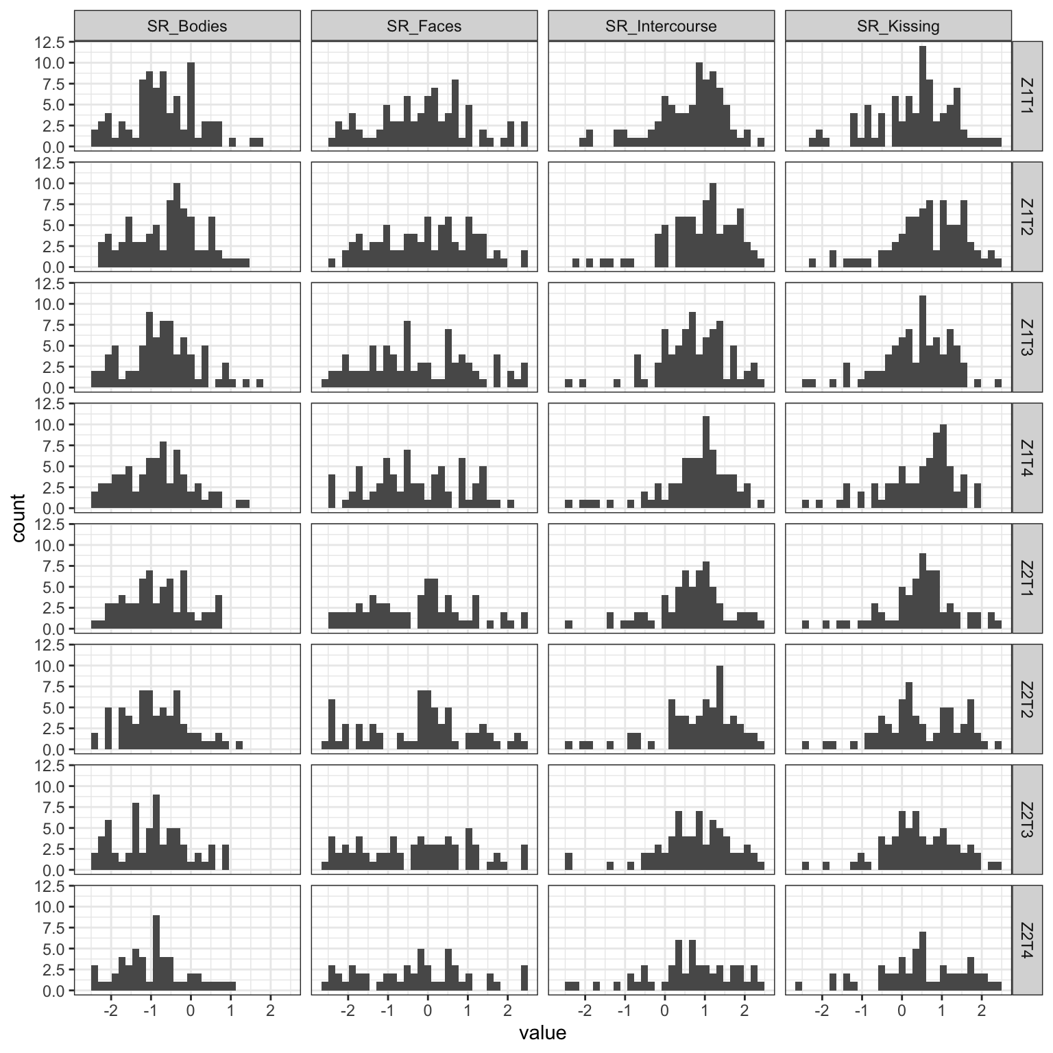
Figure 1: Distributions of the outcome visual analogue scale ratings over time. (Z=cycle, T=time point)
Hmm, the generalizability of within person variations averaged over items is zero, so maybe aggregating is not a good idea. However, a multivariate model would allow me to do some partial pooling across outcomes, so went with that.
A multivariate model
So, in the below model, I:
- logged estradiol and progesterone, this way I did not have to include the estradiol-progesterone ratio in the model
- omitted testosterone, at least as a first step
- allowed slopes to vary by person and cycle
- allowed correlations across outcomes, both for the residuals and the varying slopes and intercepts
Show code
library(brms)
library(cmdstanr)
library(tidybayes)
knitr::opts_chunk$set(tidy = FALSE)
options(brms.backend = "cmdstanr",  # I use the cmdstanr backend
        mc.cores = 8,
        brms.threads = 2,           # which allows me to multithread
        brms.file_refit = "on_change", # this is useful when doing iterative model building, though it can misfire, be careful
        width = 8000)

m1mv0 <- brm(mvbind(SR_Faces, SR_Bodies, SR_Kissing, SR_Intercourse) ~  cycle + (1 |i|ID) + (1 |c|ID:cycle), cycles_long %>% drop_na(logOESTR, logPROG),
            iter = 6000, file = "m1mv0",
            control = list(adapt_delta = 0.99))

m1mv <- brm(mvbind(SR_Faces, SR_Bodies, SR_Kissing, SR_Intercourse) ~ log(OESTR) + log(PROG) + cycle + (1 + log(OESTR) + log(PROG)|i|ID) + (1 + log(OESTR) + log(PROG)|c|ID:cycle), cycles_long,
            iter = 6000, file = "m1mv",
            control = list(adapt_delta = 0.99))
Model output and comparison to null model
Show code
options(width = 8000)
m1mv
Family: MV(gaussian, gaussian, gaussian, gaussian)
Links: mu = identity; sigma = identity
mu = identity; sigma = identity
mu = identity; sigma = identity
mu = identity; sigma = identity
Formula: SR_Faces ~ log(OESTR) + log(PROG) + cycle + (1 + log(OESTR) + log(PROG) | i | ID) + (1 + log(OESTR) + log(PROG) | c | ID:cycle)
SR_Bodies ~ log(OESTR) + log(PROG) + cycle + (1 + log(OESTR) + log(PROG) | i | ID) + (1 + log(OESTR) + log(PROG) | c | ID:cycle)
SR_Kissing ~ log(OESTR) + log(PROG) + cycle + (1 + log(OESTR) + log(PROG) | i | ID) + (1 + log(OESTR) + log(PROG) | c | ID:cycle)
SR_Intercourse ~ log(OESTR) + log(PROG) + cycle + (1 + log(OESTR) + log(PROG) | i | ID) + (1 + log(OESTR) + log(PROG) | c | ID:cycle)
Data: cycles_long (Number of observations: 551)
Draws: 4 chains, each with iter = 6000; warmup = 3000; thin = 1;
total post-warmup draws = 12000
Group-Level Effects:
~ID (Number of levels: 87)
Estimate Est.Error l-95% CI u-95% CI Rhat Bulk_ESS Tail_ESS
sd(SRFaces_Intercept) 0.91 0.18 0.52 1.24 1.00 1754 954
sd(SRFaces_logOESTR) 0.09 0.05 0.01 0.18 1.01 384 1451
sd(SRFaces_logPROG) 0.06 0.03 0.01 0.12 1.00 1262 1162
sd(SRBodies_Intercept) 0.71 0.09 0.52 0.89 1.00 3926 3637
sd(SRBodies_logOESTR) 0.03 0.02 0.00 0.09 1.01 802 1388
sd(SRBodies_logPROG) 0.03 0.02 0.00 0.07 1.00 2272 4007
sd(SRKissing_Intercept) 0.80 0.11 0.60 1.05 1.00 5869 6772
sd(SRKissing_logOESTR) 0.05 0.03 0.00 0.12 1.00 1228 3401
sd(SRKissing_logPROG) 0.03 0.02 0.00 0.07 1.00 2925 5597
sd(SRIntercourse_Intercept) 0.69 0.14 0.39 0.97 1.00 4201 4153
sd(SRIntercourse_logOESTR) 0.08 0.03 0.01 0.14 1.01 1482 2455
sd(SRIntercourse_logPROG) 0.02 0.01 0.00 0.05 1.00 7089 5680
cor(SRFaces_Intercept,SRFaces_logOESTR) -0.07 0.27 -0.57 0.47 1.00 2049 5232
cor(SRFaces_Intercept,SRFaces_logPROG) 0.06 0.24 -0.44 0.52 1.00 2412 6102
cor(SRFaces_logOESTR,SRFaces_logPROG) 0.10 0.27 -0.43 0.59 1.00 2919 5583
cor(SRFaces_Intercept,SRBodies_Intercept) 0.36 0.16 0.00 0.64 1.00 1142 2225
cor(SRFaces_logOESTR,SRBodies_Intercept) 0.15 0.24 -0.35 0.59 1.00 876 1793
cor(SRFaces_logPROG,SRBodies_Intercept) 0.17 0.23 -0.30 0.59 1.00 1093 2287
cor(SRFaces_Intercept,SRBodies_logOESTR) 0.01 0.26 -0.50 0.51 1.00 12488 9042
cor(SRFaces_logOESTR,SRBodies_logOESTR) 0.02 0.27 -0.49 0.54 1.00 5779 8230
cor(SRFaces_logPROG,SRBodies_logOESTR) 0.00 0.27 -0.53 0.53 1.00 8097 8997
cor(SRBodies_Intercept,SRBodies_logOESTR) -0.01 0.27 -0.51 0.51 1.00 8516 9109
cor(SRFaces_Intercept,SRBodies_logPROG) 0.03 0.25 -0.46 0.51 1.00 11937 9061
cor(SRFaces_logOESTR,SRBodies_logPROG) -0.02 0.27 -0.53 0.51 1.00 6642 8450
cor(SRFaces_logPROG,SRBodies_logPROG) 0.02 0.27 -0.50 0.54 1.00 7737 8150
cor(SRBodies_Intercept,SRBodies_logPROG) 0.10 0.25 -0.40 0.56 1.00 12621 8147
cor(SRBodies_logOESTR,SRBodies_logPROG) 0.02 0.27 -0.51 0.54 1.00 6623 8980
cor(SRFaces_Intercept,SRKissing_Intercept) 0.40 0.16 0.05 0.67 1.00 1375 1418
cor(SRFaces_logOESTR,SRKissing_Intercept) 0.11 0.24 -0.39 0.56 1.01 1090 1814
cor(SRFaces_logPROG,SRKissing_Intercept) -0.17 0.23 -0.59 0.31 1.00 1347 1555
cor(SRBodies_Intercept,SRKissing_Intercept) 0.19 0.16 -0.14 0.46 1.00 3093 5296
cor(SRBodies_logOESTR,SRKissing_Intercept) 0.06 0.26 -0.45 0.54 1.00 1436 3259
cor(SRBodies_logPROG,SRKissing_Intercept) 0.13 0.24 -0.38 0.58 1.00 2175 4124
cor(SRFaces_Intercept,SRKissing_logOESTR) -0.03 0.26 -0.53 0.48 1.00 6664 8724
cor(SRFaces_logOESTR,SRKissing_logOESTR) -0.08 0.27 -0.57 0.46 1.00 4768 7422
cor(SRFaces_logPROG,SRKissing_logOESTR) -0.08 0.27 -0.57 0.45 1.00 5973 8418
cor(SRBodies_Intercept,SRKissing_logOESTR) 0.15 0.26 -0.38 0.61 1.00 10292 8256
cor(SRBodies_logOESTR,SRKissing_logOESTR) 0.07 0.27 -0.47 0.58 1.00 7156 8895
cor(SRBodies_logPROG,SRKissing_logOESTR) 0.06 0.27 -0.49 0.57 1.00 8805 9999
cor(SRKissing_Intercept,SRKissing_logOESTR) -0.18 0.28 -0.66 0.40 1.00 4508 8079
cor(SRFaces_Intercept,SRKissing_logPROG) -0.07 0.26 -0.54 0.45 1.00 13308 8995
cor(SRFaces_logOESTR,SRKissing_logPROG) -0.03 0.27 -0.54 0.51 1.00 8504 9278
cor(SRFaces_logPROG,SRKissing_logPROG) 0.04 0.27 -0.50 0.55 1.00 9818 8006
cor(SRBodies_Intercept,SRKissing_logPROG) -0.00 0.26 -0.49 0.50 1.00 14921 8442
cor(SRBodies_logOESTR,SRKissing_logPROG) -0.01 0.27 -0.52 0.51 1.00 7387 8837
cor(SRBodies_logPROG,SRKissing_logPROG) 0.02 0.27 -0.50 0.54 1.00 8177 9815
cor(SRKissing_Intercept,SRKissing_logPROG) -0.05 0.26 -0.53 0.47 1.00 13370 9196
cor(SRKissing_logOESTR,SRKissing_logPROG) -0.00 0.27 -0.52 0.53 1.00 7398 9032
cor(SRFaces_Intercept,SRIntercourse_Intercept) 0.02 0.20 -0.36 0.40 1.00 2583 4005
cor(SRFaces_logOESTR,SRIntercourse_Intercept) -0.03 0.24 -0.51 0.44 1.00 1166 2638
cor(SRFaces_logPROG,SRIntercourse_Intercept) -0.05 0.24 -0.52 0.41 1.00 1573 3470
cor(SRBodies_Intercept,SRIntercourse_Intercept) 0.21 0.17 -0.15 0.53 1.00 5264 7247
cor(SRBodies_logOESTR,SRIntercourse_Intercept) 0.05 0.26 -0.45 0.54 1.00 1664 3815
cor(SRBodies_logPROG,SRIntercourse_Intercept) 0.16 0.25 -0.36 0.61 1.00 2143 3525
cor(SRKissing_Intercept,SRIntercourse_Intercept) 0.46 0.19 0.03 0.75 1.00 2193 5048
cor(SRKissing_logOESTR,SRIntercourse_Intercept) 0.19 0.26 -0.35 0.66 1.00 2642 6558
cor(SRKissing_logPROG,SRIntercourse_Intercept) 0.13 0.26 -0.40 0.60 1.00 3781 7742
cor(SRFaces_Intercept,SRIntercourse_logOESTR) 0.12 0.23 -0.34 0.54 1.00 4581 6479
cor(SRFaces_logOESTR,SRIntercourse_logOESTR) 0.07 0.26 -0.44 0.57 1.00 2286 5319
cor(SRFaces_logPROG,SRIntercourse_logOESTR) 0.01 0.25 -0.48 0.50 1.00 3672 7120
cor(SRBodies_Intercept,SRIntercourse_logOESTR) -0.05 0.22 -0.48 0.39 1.00 9113 7600
cor(SRBodies_logOESTR,SRIntercourse_logOESTR) -0.04 0.27 -0.55 0.49 1.00 2956 6047
cor(SRBodies_logPROG,SRIntercourse_logOESTR) 0.10 0.26 -0.44 0.59 1.00 3664 6303
cor(SRKissing_Intercept,SRIntercourse_logOESTR) 0.29 0.23 -0.21 0.68 1.00 7440 5910
cor(SRKissing_logOESTR,SRIntercourse_logOESTR) 0.02 0.27 -0.51 0.54 1.00 4481 7853
cor(SRKissing_logPROG,SRIntercourse_logOESTR) 0.07 0.27 -0.46 0.58 1.00 5425 9041
cor(SRIntercourse_Intercept,SRIntercourse_logOESTR) -0.09 0.27 -0.58 0.46 1.00 4465 7950
cor(SRFaces_Intercept,SRIntercourse_logPROG) -0.04 0.28 -0.56 0.50 1.00 19037 8436
cor(SRFaces_logOESTR,SRIntercourse_logPROG) -0.01 0.27 -0.53 0.51 1.00 16186 8912
cor(SRFaces_logPROG,SRIntercourse_logPROG) -0.00 0.28 -0.53 0.53 1.00 14895 8501
cor(SRBodies_Intercept,SRIntercourse_logPROG) -0.03 0.28 -0.55 0.50 1.00 20543 8788
cor(SRBodies_logOESTR,SRIntercourse_logPROG) 0.00 0.28 -0.54 0.54 1.00 10941 8990
cor(SRBodies_logPROG,SRIntercourse_logPROG) -0.00 0.28 -0.55 0.53 1.00 11439 9846
cor(SRKissing_Intercept,SRIntercourse_logPROG) -0.01 0.27 -0.54 0.50 1.00 16414 9556
cor(SRKissing_logOESTR,SRIntercourse_logPROG) 0.01 0.28 -0.53 0.54 1.00 9671 9039
cor(SRKissing_logPROG,SRIntercourse_logPROG) 0.04 0.28 -0.51 0.57 1.00 8979 10350
cor(SRIntercourse_Intercept,SRIntercourse_logPROG) -0.01 0.27 -0.53 0.53 1.00 13612 10073
cor(SRIntercourse_logOESTR,SRIntercourse_logPROG) -0.04 0.27 -0.55 0.50 1.00 10481 10230
~ID:cycle (Number of levels: 155)
Estimate Est.Error l-95% CI u-95% CI Rhat Bulk_ESS Tail_ESS
sd(SRFaces_Intercept) 0.23 0.14 0.01 0.49 1.00 1060 3003
sd(SRFaces_logOESTR) 0.05 0.02 0.01 0.09 1.01 755 1774
sd(SRFaces_logPROG) 0.04 0.03 0.00 0.09 1.00 2833 5791
sd(SRBodies_Intercept) 0.20 0.08 0.02 0.34 1.00 1123 1537
sd(SRBodies_logOESTR) 0.02 0.01 0.00 0.05 1.00 676 2430
sd(SRBodies_logPROG) 0.03 0.02 0.00 0.07 1.00 1976 5255
sd(SRKissing_Intercept) 0.11 0.07 0.01 0.25 1.00 2373 4992
sd(SRKissing_logOESTR) 0.02 0.01 0.00 0.05 1.00 1464 3148
sd(SRKissing_logPROG) 0.02 0.02 0.00 0.06 1.00 4545 6123
sd(SRIntercourse_Intercept) 0.14 0.08 0.01 0.28 1.00 2539 4014
sd(SRIntercourse_logOESTR) 0.02 0.01 0.00 0.04 1.00 2537 5787
sd(SRIntercourse_logPROG) 0.02 0.02 0.00 0.06 1.00 4235 5040
cor(SRFaces_Intercept,SRFaces_logOESTR) -0.06 0.28 -0.60 0.49 1.00 3019 6296
cor(SRFaces_Intercept,SRFaces_logPROG) -0.03 0.28 -0.55 0.50 1.00 11293 8423
cor(SRFaces_logOESTR,SRFaces_logPROG) -0.01 0.27 -0.53 0.51 1.00 12835 8356
cor(SRFaces_Intercept,SRBodies_Intercept) 0.09 0.27 -0.46 0.56 1.00 2221 4411
cor(SRFaces_logOESTR,SRBodies_Intercept) 0.10 0.25 -0.42 0.55 1.00 2766 5243
cor(SRFaces_logPROG,SRBodies_Intercept) 0.10 0.27 -0.45 0.60 1.00 2287 4660
cor(SRFaces_Intercept,SRBodies_logOESTR) 0.04 0.27 -0.50 0.55 1.00 5202 7342
cor(SRFaces_logOESTR,SRBodies_logOESTR) 0.06 0.27 -0.49 0.55 1.00 5287 6875
cor(SRFaces_logPROG,SRBodies_logOESTR) 0.06 0.27 -0.49 0.58 1.00 3829 6984
cor(SRBodies_Intercept,SRBodies_logOESTR) -0.04 0.28 -0.59 0.51 1.00 8507 6344
cor(SRFaces_Intercept,SRBodies_logPROG) -0.02 0.27 -0.55 0.50 1.00 8783 8879
cor(SRFaces_logOESTR,SRBodies_logPROG) -0.04 0.27 -0.55 0.49 1.00 9136 9456
cor(SRFaces_logPROG,SRBodies_logPROG) -0.02 0.28 -0.54 0.52 1.00 8549 9224
cor(SRBodies_Intercept,SRBodies_logPROG) -0.20 0.29 -0.69 0.41 1.00 3898 7763
cor(SRBodies_logOESTR,SRBodies_logPROG) -0.11 0.29 -0.63 0.46 1.00 5296 8147
cor(SRFaces_Intercept,SRKissing_Intercept) 0.03 0.27 -0.50 0.55 1.00 7627 8351
cor(SRFaces_logOESTR,SRKissing_Intercept) 0.04 0.27 -0.49 0.54 1.00 9729 8352
cor(SRFaces_logPROG,SRKissing_Intercept) -0.02 0.27 -0.54 0.51 1.00 7009 7496
cor(SRBodies_Intercept,SRKissing_Intercept) 0.04 0.27 -0.49 0.54 1.00 8606 9138
cor(SRBodies_logOESTR,SRKissing_Intercept) 0.04 0.27 -0.50 0.56 1.00 6706 9178
cor(SRBodies_logPROG,SRKissing_Intercept) -0.01 0.28 -0.55 0.53 1.00 7502 9014
cor(SRFaces_Intercept,SRKissing_logOESTR) 0.03 0.26 -0.49 0.53 1.00 4404 7148
cor(SRFaces_logOESTR,SRKissing_logOESTR) 0.02 0.26 -0.49 0.50 1.00 6463 7900
cor(SRFaces_logPROG,SRKissing_logOESTR) -0.04 0.28 -0.56 0.50 1.00 4373 7109
cor(SRBodies_Intercept,SRKissing_logOESTR) 0.04 0.26 -0.47 0.53 1.00 7013 9063
cor(SRBodies_logOESTR,SRKissing_logOESTR) 0.04 0.27 -0.49 0.55 1.00 5720 8204
cor(SRBodies_logPROG,SRKissing_logOESTR) -0.01 0.27 -0.54 0.51 1.00 5952 7872
cor(SRKissing_Intercept,SRKissing_logOESTR) -0.05 0.28 -0.58 0.50 1.00 6173 8371
cor(SRFaces_Intercept,SRKissing_logPROG) 0.04 0.27 -0.49 0.55 1.00 12145 9111
cor(SRFaces_logOESTR,SRKissing_logPROG) 0.06 0.28 -0.48 0.58 1.00 13327 9312
cor(SRFaces_logPROG,SRKissing_logPROG) 0.02 0.27 -0.51 0.54 1.00 12235 9822
cor(SRBodies_Intercept,SRKissing_logPROG) 0.02 0.27 -0.51 0.53 1.00 12509 9268
cor(SRBodies_logOESTR,SRKissing_logPROG) 0.01 0.28 -0.52 0.54 1.00 10632 9904
cor(SRBodies_logPROG,SRKissing_logPROG) -0.04 0.28 -0.56 0.51 1.00 9590 9562
cor(SRKissing_Intercept,SRKissing_logPROG) -0.02 0.28 -0.56 0.53 1.00 10356 10061
cor(SRKissing_logOESTR,SRKissing_logPROG) -0.03 0.28 -0.56 0.51 1.00 9963 9191
cor(SRFaces_Intercept,SRIntercourse_Intercept) -0.07 0.27 -0.58 0.47 1.00 5145 7140
cor(SRFaces_logOESTR,SRIntercourse_Intercept) -0.08 0.26 -0.56 0.44 1.00 6862 8269
cor(SRFaces_logPROG,SRIntercourse_Intercept) -0.05 0.27 -0.56 0.50 1.00 5857 7855
cor(SRBodies_Intercept,SRIntercourse_Intercept) -0.09 0.26 -0.56 0.45 1.00 5792 5964
cor(SRBodies_logOESTR,SRIntercourse_Intercept) -0.06 0.27 -0.57 0.49 1.00 6194 8864
cor(SRBodies_logPROG,SRIntercourse_Intercept) 0.07 0.28 -0.48 0.58 1.00 6205 8620
cor(SRKissing_Intercept,SRIntercourse_Intercept) 0.09 0.28 -0.46 0.59 1.00 6045 9092
cor(SRKissing_logOESTR,SRIntercourse_Intercept) 0.15 0.28 -0.42 0.65 1.00 5312 7865
cor(SRKissing_logPROG,SRIntercourse_Intercept) -0.00 0.27 -0.52 0.52 1.00 7463 10084
cor(SRFaces_Intercept,SRIntercourse_logOESTR) -0.02 0.27 -0.54 0.51 1.00 8691 8116
cor(SRFaces_logOESTR,SRIntercourse_logOESTR) -0.01 0.26 -0.51 0.50 1.00 9421 9011
cor(SRFaces_logPROG,SRIntercourse_logOESTR) -0.04 0.27 -0.55 0.50 1.00 7492 8835
cor(SRBodies_Intercept,SRIntercourse_logOESTR) -0.08 0.27 -0.58 0.47 1.00 7262 8595
cor(SRBodies_logOESTR,SRIntercourse_logOESTR) -0.06 0.27 -0.57 0.49 1.00 6478 8494
cor(SRBodies_logPROG,SRIntercourse_logOESTR) 0.06 0.28 -0.49 0.57 1.00 7140 8383
cor(SRKissing_Intercept,SRIntercourse_logOESTR) 0.07 0.28 -0.49 0.59 1.00 6995 9369
cor(SRKissing_logOESTR,SRIntercourse_logOESTR) 0.11 0.28 -0.46 0.62 1.00 6502 9009
cor(SRKissing_logPROG,SRIntercourse_logOESTR) -0.00 0.28 -0.54 0.53 1.00 7081 9351
cor(SRIntercourse_Intercept,SRIntercourse_logOESTR) -0.06 0.28 -0.60 0.48 1.00 9499 9733
cor(SRFaces_Intercept,SRIntercourse_logPROG) -0.00 0.27 -0.53 0.52 1.00 14990 9485
cor(SRFaces_logOESTR,SRIntercourse_logPROG) 0.01 0.27 -0.51 0.53 1.00 14252 9014
cor(SRFaces_logPROG,SRIntercourse_logPROG) 0.00 0.28 -0.52 0.54 1.00 12405 8696
cor(SRBodies_Intercept,SRIntercourse_logPROG) -0.03 0.27 -0.56 0.50 1.00 13054 9155
cor(SRBodies_logOESTR,SRIntercourse_logPROG) -0.02 0.28 -0.55 0.52 1.00 10884 9401
cor(SRBodies_logPROG,SRIntercourse_logPROG) 0.03 0.28 -0.52 0.56 1.00 10002 9051
cor(SRKissing_Intercept,SRIntercourse_logPROG) 0.03 0.28 -0.51 0.55 1.00 10663 10129
cor(SRKissing_logOESTR,SRIntercourse_logPROG) 0.04 0.28 -0.50 0.56 1.00 10282 10091
cor(SRKissing_logPROG,SRIntercourse_logPROG) 0.03 0.28 -0.50 0.56 1.00 8733 9824
cor(SRIntercourse_Intercept,SRIntercourse_logPROG) -0.03 0.27 -0.54 0.50 1.00 9800 10886
cor(SRIntercourse_logOESTR,SRIntercourse_logPROG) -0.01 0.28 -0.54 0.53 1.00 8420 10232
Population-Level Effects:
Estimate Est.Error l-95% CI u-95% CI Rhat Bulk_ESS Tail_ESS
SRFaces_Intercept -0.04 0.24 -0.51 0.44 1.00 9371 9434
SRBodies_Intercept -0.79 0.15 -1.09 -0.49 1.00 9116 9399
SRKissing_Intercept 0.10 0.19 -0.27 0.48 1.00 9851 9558
SRIntercourse_Intercept 0.22 0.20 -0.17 0.60 1.00 10865 9431
SRFaces_logOESTR -0.01 0.04 -0.09 0.07 1.00 11608 9730
SRFaces_logPROG -0.02 0.02 -0.06 0.03 1.00 12397 10268
SRFaces_cycleZ2 -0.15 0.09 -0.32 0.03 1.00 8394 9534
SRBodies_logOESTR 0.02 0.02 -0.02 0.07 1.00 13214 9353
SRBodies_logPROG -0.03 0.01 -0.06 -0.00 1.00 12169 9525
SRBodies_cycleZ2 -0.15 0.05 -0.25 -0.05 1.00 9394 9186
SRKissing_logOESTR 0.07 0.03 0.01 0.13 1.00 11914 10016
SRKissing_logPROG -0.03 0.02 -0.06 0.00 1.00 11387 9710
SRKissing_cycleZ2 0.05 0.05 -0.05 0.16 1.00 10076 9242
SRIntercourse_logOESTR 0.10 0.03 0.03 0.16 1.00 10294 8333
SRIntercourse_logPROG -0.03 0.02 -0.07 -0.00 1.00 11949 9636
SRIntercourse_cycleZ2 0.00 0.06 -0.10 0.12 1.00 11584 9844
Family Specific Parameters:
Estimate Est.Error l-95% CI u-95% CI Rhat Bulk_ESS Tail_ESS
sigma_SRFaces 0.60 0.02 0.55 0.64 1.00 6182 9029
sigma_SRBodies 0.35 0.01 0.33 0.38 1.00 5629 8346
sigma_SRKissing 0.46 0.02 0.43 0.50 1.00 6691 8625
sigma_SRIntercourse 0.49 0.02 0.46 0.53 1.00 7790 8743
Residual Correlations:
Estimate Est.Error l-95% CI u-95% CI Rhat Bulk_ESS Tail_ESS
rescor(SRFaces,SRBodies) 0.30 0.05 0.20 0.39 1.00 9539 9467
rescor(SRFaces,SRKissing) 0.15 0.05 0.05 0.25 1.00 8908 8678
rescor(SRBodies,SRKissing) 0.18 0.05 0.08 0.27 1.00 9600 9746
rescor(SRFaces,SRIntercourse) 0.09 0.05 -0.01 0.19 1.00 10994 9227
rescor(SRBodies,SRIntercourse) 0.14 0.05 0.04 0.24 1.00 10321 8966
rescor(SRKissing,SRIntercourse) 0.48 0.04 0.40 0.55 1.00 8200 9036
Draws were sampled using sample(hmc). For each parameter, Bulk_ESS
and Tail_ESS are effective sample size measures, and Rhat is the potential
scale reduction factor on split chains (at convergence, Rhat = 1).Show code
LOO(m1mv0, m1mv)Output of model 'm1mv0':
Computed from 12000 by 551 log-likelihood matrix
Estimate SE
elpd_loo -1662.1 53.8
p_loo 432.1 19.4
looic 3324.1 107.6
------
Monte Carlo SE of elpd_loo is NA.
Pareto k diagnostic values:
Count Pct. Min. n_eff
(-Inf, 0.5] (good) 431 78.2% 405
(0.5, 0.7] (ok) 102 18.5% 116
(0.7, 1] (bad) 16 2.9% 31
(1, Inf) (very bad) 2 0.4% 9
See help('pareto-k-diagnostic') for details.
Output of model 'm1mv':
Computed from 12000 by 551 log-likelihood matrix
Estimate SE
elpd_loo -1651.4 53.5
p_loo 509.6 21.8
looic 3302.8 107.0
------
Monte Carlo SE of elpd_loo is NA.
Pareto k diagnostic values:
Count Pct. Min. n_eff
(-Inf, 0.5] (good) 325 59.0% 777
(0.5, 0.7] (ok) 183 33.2% 204
(0.7, 1] (bad) 39 7.1% 31
(1, Inf) (very bad) 4 0.7% 13
See help('pareto-k-diagnostic') for details.
Model comparisons:
elpd_diff se_diff
m1mv 0.0 0.0
m1mv0 -10.7 7.0 As you can see if you expand the detail above, this doesn’t lead to very different conclusions.
A location-scale model
So, on analogue rating scales, you often see substantially heterogeneous variances, this is the case here too. Will accounting for it in a simple location-scale model make a difference? From here on out, I’m going to simplify and only look at one outcome (SR_Intercourse) for now. I’ll also drop the varying slopes by cycle for simplicity.
Show code
sds <- cycles_long %>% select(ID, cycle_time, starts_with("SR_")) %>% pivot_longer(-c(ID, cycle_time)) %>%
  group_by(ID, name) %>%
  summarise(sd = sd(value)) %>%
  group_by(name)


sds %>%
  arrange(sd) %>%
  ggplot(aes(sd)) +
  geom_histogram() +
  facet_wrap(~ name, scales = "free")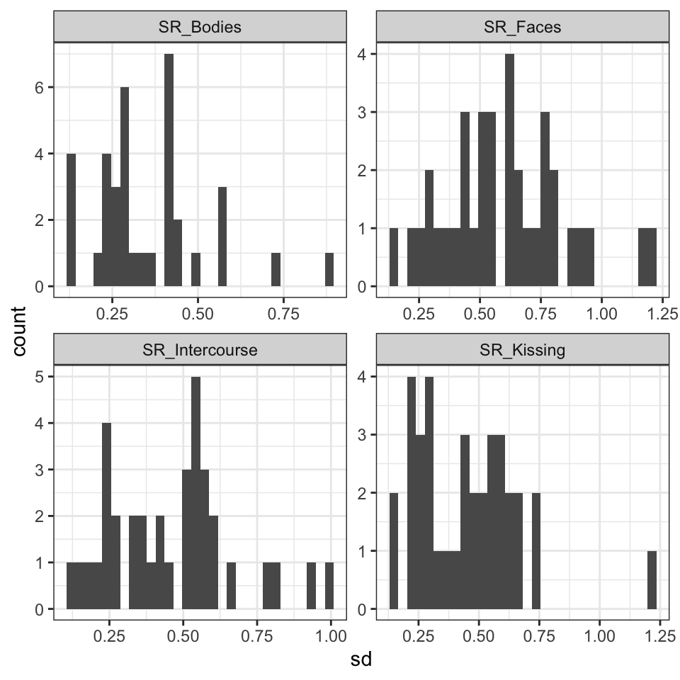
Figure 2: Heterogenity in standard deviations by person.
Model output
Show code
m1intercourse <- brm(SR_Intercourse ~ logOESTR + logPROG + cycle + (1 + logOESTR + logPROG|i|ID), cycles_long,
            iter = 4000, file = "m1intercourse")

m1intercourse_sigma <- brm(bf(SR_Intercourse ~ logOESTR + logPROG + cycle + (1 + logOESTR + logPROG|i|ID),
                        sigma ~ (1|i|ID)), cycles_long,
            iter = 6000, file = "m1intercourse_sigma",
            # file_refit = "always",
            control = list(adapt_delta = .99))
m1intercourse_sigma
Family: gaussian
Links: mu = identity; sigma = log
Formula: SR_Intercourse ~ logOESTR + logPROG + cycle + (1 + logOESTR + logPROG | i | ID)
sigma ~ (1 | i | ID)
Data: cycles_long (Number of observations: 551)
Draws: 4 chains, each with iter = 6000; warmup = 3000; thin = 1;
total post-warmup draws = 12000
Group-Level Effects:
~ID (Number of levels: 87)
Estimate Est.Error l-95% CI u-95% CI
sd(Intercept) 0.79 0.17 0.46 1.15
sd(logOESTR) 0.08 0.04 0.01 0.17
sd(logPROG) 0.02 0.01 0.00 0.05
sd(sigma_Intercept) 0.39 0.06 0.28 0.51
cor(Intercept,logOESTR) -0.19 0.39 -0.74 0.68
cor(Intercept,logPROG) 0.22 0.41 -0.66 0.86
cor(logOESTR,logPROG) -0.07 0.44 -0.82 0.77
cor(Intercept,sigma_Intercept) -0.47 0.21 -0.85 -0.02
cor(logOESTR,sigma_Intercept) 0.14 0.34 -0.57 0.74
cor(logPROG,sigma_Intercept) -0.23 0.42 -0.88 0.68
Rhat Bulk_ESS Tail_ESS
sd(Intercept) 1.00 3690 4494
sd(logOESTR) 1.01 417 1162
sd(logPROG) 1.00 6321 7354
sd(sigma_Intercept) 1.00 4169 7572
cor(Intercept,logOESTR) 1.00 1096 3026
cor(Intercept,logPROG) 1.00 13507 8678
cor(logOESTR,logPROG) 1.00 9315 9202
cor(Intercept,sigma_Intercept) 1.00 1293 2803
cor(logOESTR,sigma_Intercept) 1.00 1043 1323
cor(logPROG,sigma_Intercept) 1.01 637 2282
Population-Level Effects:
Estimate Est.Error l-95% CI u-95% CI Rhat Bulk_ESS
Intercept 0.25 0.19 -0.12 0.62 1.00 9289
sigma_Intercept -0.81 0.06 -0.92 -0.70 1.00 5269
logOESTR 0.09 0.03 0.03 0.15 1.00 9304
logPROG -0.03 0.02 -0.06 -0.00 1.00 9162
cycleZ2 0.03 0.04 -0.05 0.11 1.00 17403
Tail_ESS
Intercept 9697
sigma_Intercept 8109
logOESTR 9188
logPROG 9117
cycleZ2 9139
Draws were sampled using sample(hmc). For each parameter, Bulk_ESS
and Tail_ESS are effective sample size measures, and Rhat is the potential
scale reduction factor on split chains (at convergence, Rhat = 1).Not so!
Group mean centering
So, actually we expect the effects of estradiol and progesterone to happen on the within-person level. Differences in average levels of E and P could actually confound the relationship we’re interested in. Adjusting for this is possible using various methods (this video gives a great introduction.
We can simply subtract the group mean from logOESTR and logPROG.
Model output
Show code
cycles_long <- cycles_long %>% group_by(ID) %>%
              mutate(logOESTRm = mean(logOESTR, na.rm = T),
                     logPROGm = mean(logPROG, na.rm = T)) %>%
              mutate(logOESTR_gmc = logOESTR - mean(logOESTR, na.rm = T),
                     logPROG_gmc = logPROG - mean(logPROG, na.rm = T)) %>%
              ungroup()
cycles_long %>% select(starts_with("log")) %>% cor(use = "pairwise") %>% round(2)
logOESTR logPROG logOESTRm logPROGm logOESTR_gmc
logOESTR 1.00 0.36 0.39 0.11 0.92
logPROG 0.36 1.00 0.08 0.28 0.36
logOESTRm 0.39 0.08 1.00 0.28 0.00
logPROGm 0.11 0.28 0.28 1.00 0.00
logOESTR_gmc 0.92 0.36 0.00 0.00 1.00
logPROG_gmc 0.35 0.96 0.00 0.00 0.37
logPROG_gmc
logOESTR 0.35
logPROG 0.96
logOESTRm 0.00
logPROGm 0.00
logOESTR_gmc 0.37
logPROG_gmc 1.00Show code
m1intercoursegmc <- brm(SR_Intercourse ~ logOESTR + logPROG + cycle + (1 + logOESTR + logPROG|i|ID), cycles_long %>% group_by(ID) %>%
              mutate(logOESTR = logOESTR - mean(logOESTR, na.rm = T),
                     logPROG = logPROG - mean(logPROG, na.rm = T)) %>%
              ungroup(),
            iter = 4000, file = "m1intercoursegmc")
m1intercoursegmc
Family: gaussian
Links: mu = identity; sigma = identity
Formula: SR_Intercourse ~ logOESTR + logPROG + cycle + (1 + logOESTR + logPROG | i | ID)
Data: cycles_long %>% group_by(ID) %>% mutate(logOESTR = (Number of observations: 551)
Draws: 4 chains, each with iter = 4000; warmup = 2000; thin = 1;
total post-warmup draws = 8000
Group-Level Effects:
~ID (Number of levels: 87)
Estimate Est.Error l-95% CI u-95% CI Rhat
sd(Intercept) 0.81 0.07 0.69 0.95 1.00
sd(logOESTR) 0.07 0.04 0.00 0.17 1.00
sd(logPROG) 0.02 0.01 0.00 0.05 1.00
cor(Intercept,logOESTR) 0.37 0.37 -0.53 0.92 1.00
cor(Intercept,logPROG) 0.09 0.46 -0.82 0.87 1.00
cor(logOESTR,logPROG) -0.05 0.50 -0.88 0.87 1.00
Bulk_ESS Tail_ESS
sd(Intercept) 1728 3282
sd(logOESTR) 2570 3237
sd(logPROG) 4973 4970
cor(Intercept,logOESTR) 8913 5207
cor(Intercept,logPROG) 12655 5410
cor(logOESTR,logPROG) 8904 6668
Population-Level Effects:
Estimate Est.Error l-95% CI u-95% CI Rhat Bulk_ESS Tail_ESS
Intercept 0.74 0.09 0.56 0.92 1.00 945 2056
logOESTR 0.10 0.03 0.03 0.17 1.00 10853 6651
logPROG -0.03 0.02 -0.07 0.00 1.00 11128 5939
cycleZ2 -0.00 0.05 -0.09 0.09 1.00 12906 6139
Family Specific Parameters:
Estimate Est.Error l-95% CI u-95% CI Rhat Bulk_ESS Tail_ESS
sigma 0.51 0.02 0.48 0.54 1.00 8185 5933
Draws were sampled using sample(hmc). For each parameter, Bulk_ESS
and Tail_ESS are effective sample size measures, and Rhat is the potential
scale reduction factor on split chains (at convergence, Rhat = 1).Well, this makes little if any difference, which makes sense considering that there isn’t much between-subject variance in estradiol and progesterone to begin with.
Latent group mean centering
Being a brms lover, I’ve been looking for an excuse to try Matti Vuorre’s implementation of latent group mean centering in brms. So, here goes. Edit: I’ve confirmed through more simulations that this approach does not work.
Model output
Show code
latent_formula <- bf(
  SR_Intercourse ~ intercept +
    blogOESTR*(logOESTR - logOESTRlm), # lm = latent mean,
  intercept + blogOESTR + logOESTRlm ~ 1 + (1 | ID),
  nl = TRUE
) +
  gaussian()

p <- get_prior(latent_formula, data = cycles_long) %>%
  mutate(
    prior = case_when(
      class == "b" & coef == "Intercept" ~ "normal(0, 1)",
      class == "sd" & coef == "Intercept" ~ "student_t(7, 0, 1)",
      TRUE ~ prior
    )
  )

fit_latent <- brm(
  latent_formula,
  data = cycles_long,
  prior = p,
  iter = 4000,
  cores = 8, chains = 4, threads = 2,
  backend = "cmdstanr",
  control = list(adapt_delta = 0.99),
  file = "brm-fit-latent-mean-centered3"
)

fit_latent
Family: gaussian
Links: mu = identity; sigma = identity
Formula: SR_Intercourse ~ intercept + blogOESTR * (logOESTR - logOESTRlm)
intercept ~ 1 + (1 | ID)
blogOESTR ~ 1 + (1 | ID)
logOESTRlm ~ 1 + (1 | ID)
Data: cycles_long (Number of observations: 562)
Draws: 4 chains, each with iter = 4000; warmup = 2000; thin = 1;
total post-warmup draws = 8000
Group-Level Effects:
~ID (Number of levels: 87)
Estimate Est.Error l-95% CI u-95% CI Rhat
sd(intercept_Intercept) 0.57 0.21 0.07 0.86 1.03
sd(blogOESTR_Intercept) 0.08 0.03 0.01 0.14 1.02
sd(logOESTRlm_Intercept) 1.25 1.30 0.04 5.08 1.02
Bulk_ESS Tail_ESS
sd(intercept_Intercept) 255 400
sd(blogOESTR_Intercept) 347 1040
sd(logOESTRlm_Intercept) 224 111
Population-Level Effects:
Estimate Est.Error l-95% CI u-95% CI Rhat
intercept_Intercept 0.36 0.24 -0.09 0.83 1.01
blogOESTR_Intercept 0.06 0.04 -0.01 0.13 1.01
logOESTRlm_Intercept 0.05 1.01 -1.94 2.04 1.00
Bulk_ESS Tail_ESS
intercept_Intercept 444 389
blogOESTR_Intercept 748 618
logOESTRlm_Intercept 1151 1038
Family Specific Parameters:
Estimate Est.Error l-95% CI u-95% CI Rhat Bulk_ESS Tail_ESS
sigma 0.51 0.02 0.48 0.54 1.00 8720 5997
Draws were sampled using sample(hmc). For each parameter, Bulk_ESS
and Tail_ESS are effective sample size measures, and Rhat is the potential
scale reduction factor on split chains (at convergence, Rhat = 1).Edit: Here’s an approach that does work.
Model output
Show code
cycles_long <- cycles_long %>% group_by(ID) %>%
              mutate(logOESTR2 = logOESTR,
                     seOE = sd(logOESTR, na.rm = T)/sum(!is.na(logOESTR)),
                     seP = sd(logPROG, na.rm = T)/sum(!is.na(logOESTR)),
                     logPROG2 = logPROG)

fit_latent <- brm(
  bf(SR_Intercourse ~ logOESTR + logPROG +
       mi(logOESTR2) + mi(logPROG2) +
    cycle + (1 + logOESTR + logPROG|i|ID)) +
  bf(logPROG2 | mi(seP) ~ 1 + (1|ID)) +
  bf(logOESTR2 | mi(seOE) ~ 1 + (1|ID)) +
    set_rescor(FALSE), data = cycles_long,
            iter = 4000, file = "m1intercoursegmcmi")
fit_latent
Family: MV(gaussian, gaussian, gaussian)
Links: mu = identity; sigma = identity
mu = identity; sigma = identity
mu = identity; sigma = identity
Formula: SR_Intercourse ~ logOESTR + logPROG + mi(logOESTR2) + mi(logPROG2) + cycle + (1 + logOESTR + logPROG | i | ID)
logPROG2 | mi(seP) ~ 1 + (1 | ID)
logOESTR2 | mi(seOE) ~ 1 + (1 | ID)
Data: cycles_long (Number of observations: 551)
Draws: 4 chains, each with iter = 4000; warmup = 2000; thin = 1;
total post-warmup draws = 8000
Group-Level Effects:
~ID (Number of levels: 87)
Estimate
sd(SRIntercourse_Intercept) 0.68
sd(SRIntercourse_logOESTR) 0.07
sd(SRIntercourse_logPROG) 0.02
sd(logPROG2_Intercept) 0.07
sd(logOESTR2_Intercept) 0.08
cor(SRIntercourse_Intercept,SRIntercourse_logOESTR) 0.04
cor(SRIntercourse_Intercept,SRIntercourse_logPROG) 0.06
cor(SRIntercourse_logOESTR,SRIntercourse_logPROG) -0.04
Est.Error
sd(SRIntercourse_Intercept) 0.19
sd(SRIntercourse_logOESTR) 0.04
sd(SRIntercourse_logPROG) 0.01
sd(logPROG2_Intercept) 0.05
sd(logOESTR2_Intercept) 0.05
cor(SRIntercourse_Intercept,SRIntercourse_logOESTR) 0.43
cor(SRIntercourse_Intercept,SRIntercourse_logPROG) 0.48
cor(SRIntercourse_logOESTR,SRIntercourse_logPROG) 0.49
l-95% CI u-95% CI
sd(SRIntercourse_Intercept) 0.28 1.04
sd(SRIntercourse_logOESTR) 0.01 0.15
sd(SRIntercourse_logPROG) 0.00 0.05
sd(logPROG2_Intercept) 0.00 0.20
sd(logOESTR2_Intercept) 0.00 0.19
cor(SRIntercourse_Intercept,SRIntercourse_logOESTR) -0.69 0.85
cor(SRIntercourse_Intercept,SRIntercourse_logPROG) -0.84 0.87
cor(SRIntercourse_logOESTR,SRIntercourse_logPROG) -0.88 0.87
Rhat Bulk_ESS
sd(SRIntercourse_Intercept) 1.00 1937
sd(SRIntercourse_logOESTR) 1.02 216
sd(SRIntercourse_logPROG) 1.00 3806
sd(logPROG2_Intercept) 1.00 4910
sd(logOESTR2_Intercept) 1.00 2290
cor(SRIntercourse_Intercept,SRIntercourse_logOESTR) 1.00 947
cor(SRIntercourse_Intercept,SRIntercourse_logPROG) 1.00 8227
cor(SRIntercourse_logOESTR,SRIntercourse_logPROG) 1.00 6669
Tail_ESS
sd(SRIntercourse_Intercept) 1606
sd(SRIntercourse_logOESTR) 832
sd(SRIntercourse_logPROG) 3384
sd(logPROG2_Intercept) 3494
sd(logOESTR2_Intercept) 2522
cor(SRIntercourse_Intercept,SRIntercourse_logOESTR) 1876
cor(SRIntercourse_Intercept,SRIntercourse_logPROG) 4660
cor(SRIntercourse_logOESTR,SRIntercourse_logPROG) 5849
Population-Level Effects:
Estimate Est.Error l-95% CI u-95% CI Rhat
SRIntercourse_Intercept 0.24 0.21 -0.17 0.65 1.00
logPROG2_Intercept 1.69 0.06 1.57 1.82 1.00
logOESTR2_Intercept 5.86 0.03 5.79 5.92 1.00
SRIntercourse_logOESTR 0.25 0.31 -0.36 0.87 1.00
SRIntercourse_logPROG -0.07 0.26 -0.58 0.45 1.00
SRIntercourse_cycleZ2 -0.00 0.05 -0.09 0.09 1.00
SRIntercourse_milogOESTR2 -0.15 0.32 -0.80 0.46 1.00
SRIntercourse_milogPROG2 0.04 0.27 -0.50 0.56 1.00
Bulk_ESS Tail_ESS
SRIntercourse_Intercept 5048 5438
logPROG2_Intercept 10305 6300
logOESTR2_Intercept 10605 6361
SRIntercourse_logOESTR 1668 2497
SRIntercourse_logPROG 863 1624
SRIntercourse_cycleZ2 11095 5934
SRIntercourse_milogOESTR2 1657 2569
SRIntercourse_milogPROG2 864 1578
Family Specific Parameters:
Estimate Est.Error l-95% CI u-95% CI Rhat
sigma_SRIntercourse 0.50 0.02 0.47 0.54 1.00
sigma_logPROG2 1.43 0.04 1.34 1.52 1.00
sigma_logOESTR2 0.77 0.02 0.73 0.82 1.00
Bulk_ESS Tail_ESS
sigma_SRIntercourse 4409 4243
sigma_logPROG2 11362 5936
sigma_logOESTR2 10387 6745
Draws were sampled using sample(hmc). For each parameter, Bulk_ESS
and Tail_ESS are effective sample size measures, and Rhat is the potential
scale reduction factor on split chains (at convergence, Rhat = 1).Imputations and lag
To get at the question, whether estradiol and progesterone have time-delayed effects on sexual desire, we would ideally like to have measured serum steroids a few days ahead. Unfortunately, this wasn’t done here (they did measure serum steroids on some other days, but did not share those data). A simple solution would be to substitute in my imputed hormones for the days two days prior to the rating task.
Model output
Show code
 Family: gaussian
  Links: mu = identity; sigma = identity
Formula: SR_Intercourse ~ est_estradiol_fc_lag2 + est_progesterone_fc_lag2 + cycle + (1 + est_estradiol_fc_lag2 + est_progesterone_fc_lag2 | i | ID)
   Data: cycles_longer (Number of observations: 570)
  Draws: 4 chains, each with iter = 6000; warmup = 3000; thin = 1;
         total post-warmup draws = 12000

Group-Level Effects:
~ID (Number of levels: 88)
                                                    Estimate
sd(Intercept)                                           0.72
sd(est_estradiol_fc_lag2)                               0.17
sd(est_progesterone_fc_lag2)                            0.03
cor(Intercept,est_estradiol_fc_lag2)                   -0.26
cor(Intercept,est_progesterone_fc_lag2)                -0.11
cor(est_estradiol_fc_lag2,est_progesterone_fc_lag2)     0.10
                                                    Est.Error
sd(Intercept)                                            0.34
sd(est_estradiol_fc_lag2)                                0.07
sd(est_progesterone_fc_lag2)                             0.02
cor(Intercept,est_estradiol_fc_lag2)                     0.47
cor(Intercept,est_progesterone_fc_lag2)                  0.49
cor(est_estradiol_fc_lag2,est_progesterone_fc_lag2)      0.47
                                                    l-95% CI u-95% CI
sd(Intercept)                                           0.10     1.40
sd(est_estradiol_fc_lag2)                               0.05     0.32
sd(est_progesterone_fc_lag2)                            0.00     0.09
cor(Intercept,est_estradiol_fc_lag2)                   -0.85     0.79
cor(Intercept,est_progesterone_fc_lag2)                -0.89     0.84
cor(est_estradiol_fc_lag2,est_progesterone_fc_lag2)    -0.79     0.89
                                                    Rhat Bulk_ESS
sd(Intercept)                                       1.00     1663
sd(est_estradiol_fc_lag2)                           1.02      651
sd(est_progesterone_fc_lag2)                        1.00     1404
cor(Intercept,est_estradiol_fc_lag2)                1.01      711
cor(Intercept,est_progesterone_fc_lag2)             1.00     4776
cor(est_estradiol_fc_lag2,est_progesterone_fc_lag2) 1.00     5148
                                                    Tail_ESS
sd(Intercept)                                           3732
sd(est_estradiol_fc_lag2)                               1688
sd(est_progesterone_fc_lag2)                            2613
cor(Intercept,est_estradiol_fc_lag2)                    2065
cor(Intercept,est_progesterone_fc_lag2)                 7047
cor(est_estradiol_fc_lag2,est_progesterone_fc_lag2)     7309

Population-Level Effects:
                         Estimate Est.Error l-95% CI u-95% CI Rhat
Intercept                    0.38      0.22    -0.03     0.82 1.00
est_estradiol_fc_lag2        0.17      0.05     0.06     0.27 1.00
est_progesterone_fc_lag2    -0.05      0.02    -0.10    -0.01 1.00
cycleZ2                     -0.03      0.05    -0.12     0.07 1.00
                         Bulk_ESS Tail_ESS
Intercept                   19032     9683
est_estradiol_fc_lag2       14482    10340
est_progesterone_fc_lag2    18940     8961
cycleZ2                     25540     7844

Family Specific Parameters:
      Estimate Est.Error l-95% CI u-95% CI Rhat Bulk_ESS Tail_ESS
sigma     0.51      0.02     0.47     0.54 1.00     4467     7815

Draws were sampled using sample(hmc). For each parameter, Bulk_ESS
and Tail_ESS are effective sample size measures, and Rhat is the potential
scale reduction factor on split chains (at convergence, Rhat = 1).
Show code
 Family: gaussian
  Links: mu = identity; sigma = identity
Formula: SR_Intercourse ~ est_estradiol_fc + est_progesterone_fc + cycle + (1 + est_estradiol_fc + est_progesterone_fc | i | ID)
   Data: cycles_longer (Number of observations: 570)
  Draws: 4 chains, each with iter = 6000; warmup = 3000; thin = 1;
         total post-warmup draws = 12000

Group-Level Effects:
~ID (Number of levels: 88)
                                          Estimate Est.Error l-95% CI
sd(Intercept)                                 0.61      0.30     0.06
sd(est_estradiol_fc)                          0.13      0.07     0.01
sd(est_progesterone_fc)                       0.04      0.03     0.00
cor(Intercept,est_estradiol_fc)              -0.13      0.48    -0.85
cor(Intercept,est_progesterone_fc)           -0.10      0.48    -0.87
cor(est_estradiol_fc,est_progesterone_fc)     0.16      0.46    -0.74
                                          u-95% CI Rhat Bulk_ESS
sd(Intercept)                                 1.28 1.00     1653
sd(est_estradiol_fc)                          0.27 1.00      812
sd(est_progesterone_fc)                       0.11 1.00     1392
cor(Intercept,est_estradiol_fc)               0.83 1.00     1217
cor(Intercept,est_progesterone_fc)            0.84 1.00     3423
cor(est_estradiol_fc,est_progesterone_fc)     0.91 1.00     3410
                                          Tail_ESS
sd(Intercept)                                 1468
sd(est_estradiol_fc)                          1813
sd(est_progesterone_fc)                       3218
cor(Intercept,est_estradiol_fc)               1719
cor(Intercept,est_progesterone_fc)            5540
cor(est_estradiol_fc,est_progesterone_fc)     5403

Population-Level Effects:
                    Estimate Est.Error l-95% CI u-95% CI Rhat
Intercept               0.15      0.23    -0.30     0.59 1.00
est_estradiol_fc        0.20      0.06     0.08     0.31 1.00
est_progesterone_fc    -0.04      0.02    -0.08     0.01 1.00
cycleZ2                -0.03      0.05    -0.12     0.06 1.00
                    Bulk_ESS Tail_ESS
Intercept              14741     9070
est_estradiol_fc       10393     4474
est_progesterone_fc    10516     2249
cycleZ2                18084     8375

Family Specific Parameters:
      Estimate Est.Error l-95% CI u-95% CI Rhat Bulk_ESS Tail_ESS
sigma     0.51      0.02     0.48     0.55 1.00     5034     2081

Draws were sampled using sample(hmc). For each parameter, Bulk_ESS
and Tail_ESS are effective sample size measures, and Rhat is the potential
scale reduction factor on split chains (at convergence, Rhat = 1).
Directionally, the same-day imputed hormones has a slightly stronger relationship with SR_Intercourse for oestradiol, and the two-day lag imputation has a slightly stronger relationship with progesterone. Not much that can be concluded at this sample size though.
Latent lag
Just using the imputations leaves money on the table though. Next, I thought I would use the strong relationship between imputed hormones and measured hormones to impute the missing values two days prior (and thereby carry forward the inherent uncertainty in imputation plus the individual differences, what little there are).
I thought I needed only to use the syntactic sugar for missing variables in brms (mi()). After some reshaping magic, I thought I had it, but, nope, it took forever to fit2. And I’ve never seen that many warnings from a Stan model before. I did not succeed in fixing them with the usual tricks (more informative priors, inits, playing with control parameters).
Edit: Sleeping on it, the solution came to me in a dream.3. That solution did not completely fix the model either though. What did it was rereading the brms vignette on missing values and noticing that Paul adds the | mi() also for the main response. This is necessary so brms won’t drop the rows in which the response is missing. I think you can get away with not doing so, if there is overlap, but in my case there was zero overlap (all values that had an outcome did not have lagged steroid measures). So, I added | mi() to by response SR_Intercourse.
Model output
Show code
mis_imp_formula = bf(SR_Intercourse | mi() ~ mi(logOESTR_lag2) + mi(logPROG_lag2) + cycle + (1|ID)) +
  bf(logOESTR_lag2 | mi() ~ est_estradiol_fc_lag2 + (1|ID)) +
  bf(logPROG_lag2 | mi() ~ est_progesterone_fc_lag2 + (1|ID)) +
    set_rescor(FALSE)

p <- get_prior(mis_imp_formula, data = cycles_longer) %>%
  mutate(
    prior = case_when(
      class == "b" & coef == "Intercept" ~ "normal(0, 2)",
      class == "b"  ~ "normal(0, 1)",
      class == "sd" & coef == "Intercept" ~ "student_t(3, 0, 0.5)",
      TRUE ~ prior
    )
  )


m1lag <- brm(
  mis_imp_formula,
  cycles_longer,
  iter = 4000,
  init = 0,
  file = "m1_impute_latent",
  control = list(adapt_delta = 0.99, max_treedepth = 15),
  prior = p
  )
Instead, I took a leaf out of Matti Vuorre’s book and tried my hand at the nonlinear formula syntax. I find this much less convenient to specify and harder to think about4.
It worries me that the results of the latent lag model are more like the results of the imputations without lag than of those with lag. So maybe I didn’t specify the nonlinear model correctly.
Edit: I slept on it and I did not, so I’ve cut it here. You can see it on Github if you wish.
Bringing it all together
Show code
draws <- bind_rows(
  latent_impute_lag2 = m1lag %>% gather_draws(`bsp_SRIntercourse_milog.+`, regex = T) %>% mutate(.variable = str_replace(str_replace(.variable, "bsp_SRIntercourse_mi", "b_"), "_lag2", "")),
  imputed_lag2 = m1_lagi %>% gather_draws(`b_est.+`, regex = T) %>% mutate(.variable = str_replace(str_replace(.variable, "est_estradiol_fc_lag2", "logOESTR"), "est_progesterone_fc_lag2", "logPROG")),
  imputed = m1_i %>% gather_draws(`b_est.+`, regex = T) %>% mutate(.variable = str_replace(str_replace(.variable, "est_estradiol_fc", "logOESTR"), "est_progesterone_fc", "logPROG")),
  latent_group_mean_centered = fit_latent %>% gather_draws(`b_SRIntercourse_log[A-Z]+`, regex = T) %>% mutate(.variable = str_replace(str_replace(.variable, "b_SRIntercourse_", "b_"), "_Intercept", "")),
  group_mean_centered = m1intercoursegmc %>% gather_draws(`b_log.+`, regex = T),
  location_scale = m1intercourse_sigma %>% gather_draws(`b_log.+`, regex = T),
  multivariate = m1mv %>% gather_draws(`b_SRIntercourse_log.+`, regex = T) %>% mutate(.variable = str_replace(.variable, "b_SRIntercourse_", "b_")),
  raw = m1intercourse %>% gather_draws(`b_log.+`, regex = T), .id = "model") %>%   mutate(model = fct_inorder(factor(model)))
draws <- draws %>% group_by(model, .variable) %>%
  mean_hdci(.width = c(.95, .99)) %>%
  ungroup()

ggplot(draws, aes(y = .variable, x = .value, xmin = .lower, xmax = .upper,
                  color = model)) +
  geom_pointinterval(position = position_dodge(width = .4)) +
  geom_vline(xintercept = 0, linetype = 'dashed') +
  scale_color_discrete(breaks = rev(levels(draws$model))) +
  theme_bw() +
  theme(legend.position = c(0.99,0.99),
        legend.justification = c(1,1))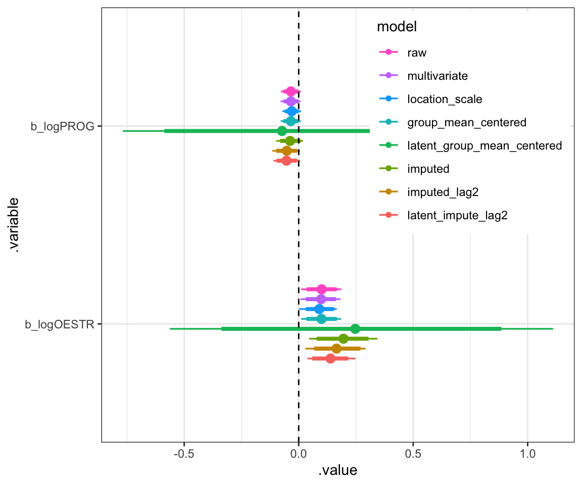
Figure 3: Non-varying slopes for log estradiol and log progesterone
“Conclusion”
In summary, I would say my different analyses did not yield very different conclusions at this sample size. If the authors had shared even more data, maybe slightly cooler reanalyses would be possible. Who knows maybe that twofold change in the effect size for estradiol when bringing in imputations and lags is real.
I ended up not bothering to bring it all together in one model, but would be interested to see what happens if you, dear reader, give it a go. Given the rest of the literature, I still put stock in a peri-ovulatory sexual desire peak, but I think this is more evidence that we all should design studies to detect small effects (here and most elsewhere in psychology) and effect heterogeneity (especially here).
Cycle researchers have recently started sharing data more widely. It’s cool to see this catch on even in medicine and I hope it continues.5 I think there are interesting substantive and statistical questions both remaining to be answered in this research.
Things I didn’t do or that still confuse me
- I didn’t do any model comparisons here.
- I never brought it all together in one multivariate location-scale model with imputations and lags
- I didn’t do any group mean centering at the level of the cycle.
- It confuses me that the results of the latent lag model are more like the results of the imputations without lag than of those with lag.
their previous publications on different outcomes in the same study unfortunately didn’t do so↩︎
which, according to the first folk theorem of statistical computing, means there’s something wrong with my model↩︎
I had confused which imputations to use as predictors and should have used the lagged ones.↩︎
If I wanted to be mean, I’d say it feels a little like MPlus with those very strict rules about how variables and parameters can be named.↩︎
It would be extra cool if preregistration catches on there outside the narrow remit of clinical trials too.↩︎