Sometimes, once we have a new concept, we see it everywhere. For me, this recently happened with the concept of Berkson error. The original paper is very readable. If, like me, you haven’t noticed this concept before, maybe you’ll also recognize it around you soon.
Let’s say, you want to measure how much müsli I eat for breakfast, I pour it into my bowl and you weigh my bowl before I eat it. The measured weight depends on the true weight (T -> X). The error of the scale means your measured value is slightly off the true value. Sometimes, it might be a bit high, sometimes it will be a bit low, but the error is unrelated to T. This is classical measurement error, very familiar to psychologists.
However, if you continue your research into my müsli consumption by assigning me experimentally assigned portion sizes, something flips. Now, you’ll pour müsli into the bowl until it’s exactly 30 grams (if you want me to have a bad day) or 60 grams (if you want me to have a good day). If after your initial pour, the scale shows 25 grams, you’ll add more until it shows 30 grams. But the scale still has error, sometimes it’s a bit high, sometimes it’s a bit low. Maybe when it showed 25 grams, it truly was already at 30 grams. What has changed is that now the true value is dependent on the measured value (X -> T) and the error is independent of X, not of T.
Does this matter? In fact, I’ve come across this problem several times, even outside the important field of müsli research.
I have worked with imputed or synthetic estimates a few times. In my work on fertile window effects, we used the imputed probability of being in the fertile window (courtesy of Gangestad et al. 2016). In my work on steroid hormones across the cycle, I imputed serum sex steroids from menstrual cycle position. And recently, with Björn Hommel, we worked on synthetic estimates for correlations between survey items.
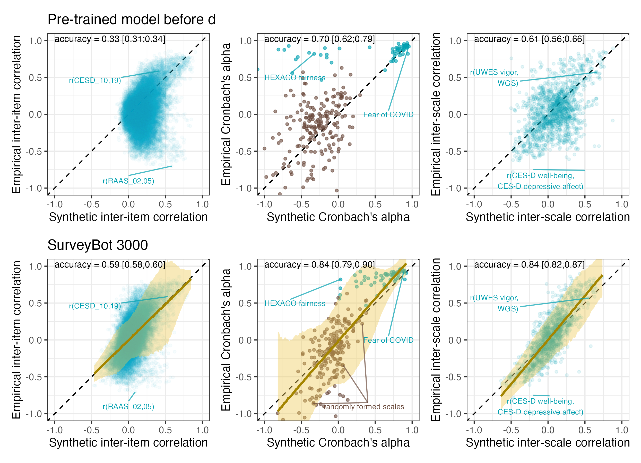
What these estimates have in common is that they come from a regression model, i.e. they are predicted true values. Also, none of them are free of error. Initially, I thought this error would need to be modelled (e.g, through SEM or errors-in-variables) if these estimates were to be used as predictors. Through simulations, I learned that this was not the case, their effects were unbiased. I understood this had something to do with the fact that the regression basically “shrunk” the estimates, but I didn’t have a name for the problem.
Fortunately, LLMs make it easy to discover names you don’t know. So, recently, when Stefan Schmukle asked me why the slopes of our synthetic correlations are 1 and not attenuated by error, I broke out into cold sweat. When Stefan is befuddled, I’ve usually made a mistake. So, I made some plots and simulations together with Claude Opus 4.5 and Gemini 3 Pro and learned the name of this problem: Berkson Error1.
The TL;DR is that when you use predicted values as predictors, you have Berkson error. The predictions will be “shrunken” relative to the true values, and in the bivariate case you do not even need to correct for it. No SEM, no nothing. So, in the case of our synthetic correlations, my cold sweat was unnecessary. However, when it came to the imputed steroid estimates which will sometimes be used for multivariate analyses, I had ignored residual confounding. Fortunately, this ended up not mattering substantially.
There’s a lot of research on this, so here I’m just trying to convey the problem visually through simulations and to connect it to concepts I already had as a psychologist like shrinking values towards the mean as a function of reliability. I would be curious to understand why this concept is not more widely taught in psychology, even though we tend to be fairly attentive to measurement error, use imputations etc. I suspect it is because we’re often so focused on correlations, which still get attenuated, but I might be wrong.
Common to all scenarios
You have a predictor \(T\) (the “true score”) that affects some outcome \(Y\):
\[Y = \beta T + \varepsilon\]
But you can’t observe \(T\) directly. Instead, you observe some proxy \(X\) that’s related to \(T\) but not identical. The question is: if you regress \(Y\) on \(X\) instead of \(T\), do you get the right answer?
The answer depends on how \(X\) and \(T\) are related. In psychology, we are most familiar with the classical test theory model (Scenario 1).
Scenario 1: Classical Measurement Error
The model: \(X = T + e\), where \(e \perp T\)
You’re trying to measure \(T\), but your measurement has random noise added to it. The noise is independent of the true value. This is what happens when you use a questionnaire with random response error, or when you measure blood pressure with an imprecise device.
Show code
df_classical <- data.frame(T = T_true, X = X_classical, Y = Y)

# Subset for arrows
set.seed(42)
arrow_idx <- sample(n, 10)
df_arrows_classical <- df_classical[arrow_idx, ]

p1_classical <- ggplot(df_classical, aes(x = T, y = X)) +
  geom_point(alpha = 0.3, color = "steelblue") +
  geom_segment(data = df_arrows_classical, aes(x = T, y = T, xend = T, yend = X),
               arrow = arrow(length = unit(0.15, "cm")), color = "red", linewidth = 0.8) +
  geom_abline(slope = 1, intercept = 0, linetype = "dashed", linewidth = 1) +
  labs(title = "Classical Error: X = T + e",
       subtitle = "",
       x = "True score (T)", y = "Observed (X)") +
  coord_fixed()

p2_classical <- ggplot(df_classical, aes(x = X, y = Y)) +
  geom_point(alpha = 0.3, color = "steelblue") +
  geom_segment(data = df_arrows_classical, aes(x = T, y = Y, xend = X, yend = Y),
               arrow = arrow(length = unit(0.15, "cm")), color = "red", linewidth = 0.8) +
  geom_smooth(method = "lm", se = FALSE, color = "red", linewidth = 1) +
  geom_abline(slope = beta_true, intercept = 0, linetype = "dashed", linewidth = 1) +
  labs(title = paste0("Regressing Y on X: β = ", round(beta_classical, 3)),
       subtitle = paste0("True β = ", beta_true, " (dashed line). Arrows show how error pushes X away from T."),
       x = "Observed (X)", y = "Outcome (Y)")

p1_classical + p2_classical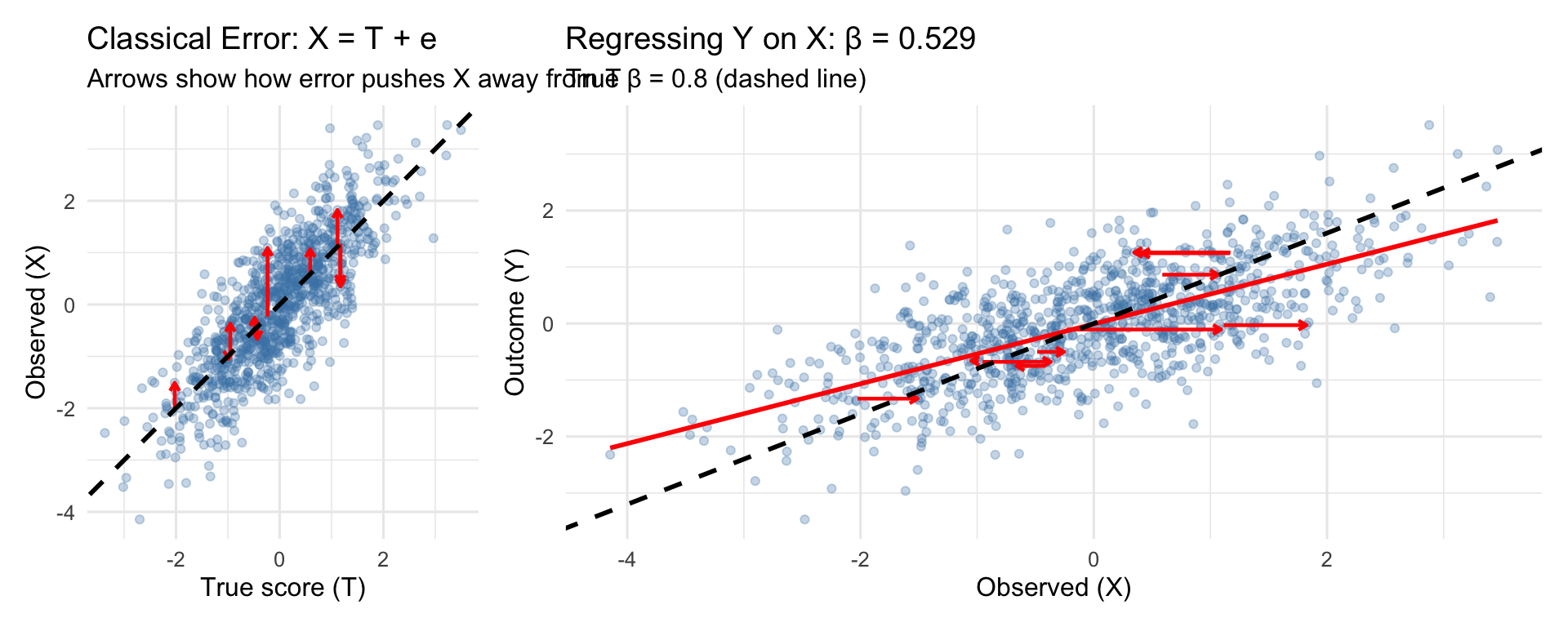
What happened? The slope is attenuated (biased toward zero). The estimated \(\hat{\beta} =\) 0.553 is smaller than the true \(\beta =\) 0.8.
Why? The noise in \(X\) is uncorrelated with \(Y\), so it just adds scatter. But crucially, the noise inflates \(\text{Var}(X)\) without increasing \(\text{Cov}(X, Y)\). Since \(\hat{\beta} = \text{Cov}(X,Y) / \text{Var}(X)\), the denominator gets bigger and the slope shrinks.
The attenuation factor is exactly the reliability: \(\hat{\beta} = \beta \times \frac{\text{Var}(T)}{\text{Var}(X)} = \beta \times \text{reliability}\)
Show numbers
Show code
Reliability: 0.657 Expected attenuation: 0.525 Actual estimate: 0.553 Show code
# Simulation function for classical error
sim_classical <- function(n = 3000, beta_true = 0.8, error_sd = 0.7) {
  T_true <- rnorm(n)
  epsilon <- rnorm(n, sd = 0.5)
  Y <- beta_true * T_true + epsilon
  X_classical <- T_true + rnorm(n, sd = error_sd)
  fit <- lm(Y ~ X_classical)
  ci <- confint(fit)[2, ]
  list(estimate = coef(fit)[2], ci_lower = ci[1], ci_upper = ci[2])
}

set.seed(123)
coverage_classical <- run_coverage_sim(sim_classical, n_sims = 1000, true_beta = beta_true)
cat("Coverage (95% CI includes true β):", round(coverage_classical$coverage * 100, 1), "%\n")
Coverage (95% CI includes true β): 0 %Mean estimate: 0.538 Bias: -0.262 Do you need to correct this? Yes. This is what errors-in-variables (EIV) regression or SEM with latent variables are designed to fix.
Scenario 2: Berkson Error
The model: \(T = X + e\), where \(e \perp X\)
This looks similar but is fundamentally different. Here, \(X\) is a prediction of \(T\), and \(T\) is the prediction plus some residual. The residual is independent of the prediction (by construction, if \(X\) comes from a regression model).
This happens when:
- You give patients a medication that you weighed to be 500mg, but your scale is imprecise ±10mg. The true value is what the patient gets (496mg, 505mg), but you measured out 500mg.
- You use predicted values from a regression model as your predictor
- You assign group means to individuals (e.g., average exposure for a job category)
- Our synthetic correlation estimates which are from a fine-tuned transformer model
- Imputed values like my serum steroid example
Show code
# Berkson error via regression prediction
# We have true T, but we only observe some proxy Z
# We regress T on Z to get predicted values X

set.seed(123)

# True score (same as other scenarios for comparability)
T_berkson <- rnorm(n, mean = 0, sd = 1)

# Some auxiliary variable correlated with T (e.g., cycle day, group assignment)
# This is what we actually observe and use to predict T
Z <- T_berkson + rnorm(n, mean = 0, sd = 1)

# Regress T on Z to get predicted values
# In practice, this regression is done on training data or prior literature
model_berkson <- lm(T_berkson ~ Z)
X_berkson <- fitted(model_berkson)

# By OLS construction: residuals are orthogonal to fitted values
# i.e., T = X + e where e ⊥ X

# Outcome based on true score
Y_berkson <- beta_true * T_berkson + rnorm(n, mean = 0, sd = 0.5)

# Regression using the prediction
fit_berkson <- lm(Y_berkson ~ X_berkson)
beta_berkson <- coef(fit_berkson)[2]

# Oracle regression (for comparison)
fit_berkson_oracle <- lm(Y_berkson ~ T_berkson)
beta_berkson_oracle <- coef(fit_berkson_oracle)[2]
Show code
df_berkson <- data.frame(T = T_berkson, X = X_berkson, Y = Y_berkson)

# Subset for arrows - show how X is shrunk relative to T
set.seed(42)
arrow_idx <- sample(n, 10)
df_arrows_berkson <- df_berkson[arrow_idx, ]

p1_berkson <- ggplot(df_berkson, aes(x = T, y = X)) +
  geom_point(alpha = 0.3, color = "forestgreen") +
  geom_segment(data = df_arrows_berkson, aes(x = T, y = T, xend = T, yend = X),
               arrow = arrow(length = unit(0.15, "cm")), color = "red", linewidth = 0.8) +
  geom_abline(slope = 1, intercept = 0, linetype = "dashed", linewidth = 1) +
  labs(title = "Berkson Error: T = X + e",
       subtitle = "Arrows show how X is shrunk toward zero",
       x = "True score (T)", y = "Predicted (X)") +
  coord_fixed()

p2_berkson <- ggplot(df_berkson, aes(x = X, y = Y)) +
  geom_point(alpha = 0.3, color = "forestgreen") +
  geom_segment(data = df_arrows_berkson, aes(x = T, y = Y, xend = X, yend = Y),
               arrow = arrow(length = unit(0.15, "cm")), color = "red", linewidth = 0.8) +
  geom_smooth(method = "lm", se = FALSE, color = "red", linewidth = 1) +
  geom_abline(slope = beta_true, intercept = 0, linetype = "dashed", linewidth = 1) +
  labs(title = paste0("Regressing Y on X: β = ", round(beta_berkson, 3)),
       subtitle = paste0("True β = ", beta_true, " (dashed line)"),
       x = "Predicted (X)", y = "Outcome (Y)")

p1_berkson + p2_berkson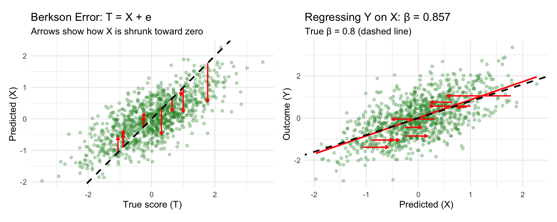
As you can see, the slope is correct! \(\hat{\beta} =\) 0.793 \(\approx\) 0.8. The key is that the error \(e\) is independent of the predictor \(X\). This means OLS assumptions are satisfied. Yes, there’s “error” in the sense that \(X \neq T\), but it’s the right kind of error.
Show numbers
Show code
# Simulation function for Berkson error
sim_berkson <- function(n = 3000, beta_true = 0.8, z_error_sd = 1) {
  T_true <- rnorm(n)
  Z <- T_true + rnorm(n, sd = z_error_sd)

  # Calculate theoretical slope for X = E[T|Z]
  # Cov(T,Z) = Var(T) = 1
  # Var(Z) = Var(T) + Var(e) = 1 + z_error_sd^2
  slope_theoretical <- 1 / (1 + z_error_sd^2)
  X_berkson <- slope_theoretical * Z

  epsilon <- rnorm(n, sd = 0.5)
  Y <- beta_true * T_true + epsilon
  fit <- lm(Y ~ X_berkson)
  ci <- confint(fit)[2, ]
  list(estimate = coef(fit)[2], ci_lower = ci[1], ci_upper = ci[2])
}

set.seed(123)
coverage_berkson <- run_coverage_sim(sim_berkson, n_sims = 1000, true_beta = beta_true)
cat("Coverage (95% CI includes true β):", round(coverage_berkson$coverage * 100, 1), "%\n")
Coverage (95% CI includes true β): 96.1 %Mean estimate: 0.802 Bias: 0.002 The coverage is close to nominal (96.1%) because the estimate is unbiased.2
Mathematically: \[\text{Cov}(X, Y) = \text{Cov}(X, \beta T + \varepsilon) = \beta \text{Cov}(X, X + e) = \beta \text{Var}(X)\]
So \(\hat{\beta} = \text{Cov}(X, Y) / \text{Var}(X) = \beta\). No attenuation!
So, you don’t need to do further correction (e.g., using SEM or errors-in-variables). Using the predicted values directly gives you unbiased slopes. The only cost is wider standard errors (because \(\text{Var}(X) < \text{Var}(T)\)).
Scenario 3: Kelley’s formula
Now, you might ask (I did at least): Why do we bother with complex models like errors-in-variables and SEM when we can just shrink the number? In psychology, we actually do this sometimes, using Kelley’s formula. But this is mainly used in univariate use cases like diagnostics and rarely connected to the concept of shrinkage elsewhere in statistics in our textbooks, leading to some confusion. Stefan wrote about this because there’s a widespread misunderstanding about how to calculate confidence intervals for such shrunk scores.
The model: \(X^* = \lambda \cdot (T + e)\), where \(e \perp T\)
This is what happens when you try to “correct” classical measurement error by shrinking the observed values toward the mean. The idea is: if \(X = T + e\) has error, maybe multiplying by the reliability \(\lambda = \text{Var}(T)/\text{Var}(X)\) will fix it?
Show code
# Start with classical error
e_shrink <- rnorm(n, mean = 0, sd = 0.7)
X_raw <- T_true + e_shrink

# "Correct" by multiplying by reliability (Kelley formula)
reliability_shrink <- var(T_true) / var(X_raw)
X_shrunk <- reliability_shrink * X_raw + (1 - reliability_shrink) * mean(X_raw)

# Regression
fit_shrunk <- lm(Y ~ X_shrunk)
beta_shrunk <- coef(fit_shrunk)[2]
Show code
df_shrink <- data.frame(T = T_true, X_raw = X_raw, X = X_shrunk, Y = Y)

# Subset for arrows
set.seed(42)
arrow_idx <- sample(n, 10)
df_arrows_shrink <- df_shrink[arrow_idx, ]

p1_shrink <- ggplot(df_shrink, aes(x = T, y = X)) +
  geom_point(alpha = 0.3, color = "darkorange") +
  geom_segment(data = df_arrows_shrink, aes(x = T, y = T, xend = T, yend = X),
               arrow = arrow(length = unit(0.15, "cm")), color = "red", linewidth = 0.8) +
  geom_abline(slope = 1, intercept = 0, linetype = "dashed", linewidth = 1) +
  labs(title = "Reliability Shrinkage: X* = λ(T + e)",
       subtitle = "Arrows show combined noise + shrinkage",
       x = "True score (T)", y = "Shrunk observed (X*)") +
  coord_fixed()

p2_shrink <- ggplot(df_shrink, aes(x = X, y = Y)) +
  geom_point(alpha = 0.3, color = "darkorange") +
  geom_segment(data = df_arrows_shrink, aes(x = T, y = Y, xend = X, yend = Y),
               arrow = arrow(length = unit(0.15, "cm")), color = "red", linewidth = 0.8) +
  geom_smooth(method = "lm", se = FALSE, color = "red", linewidth = 1) +
  geom_abline(slope = beta_true, intercept = 0, linetype = "dashed", linewidth = 1) +
  labs(title = paste0("Regressing Y on X*: β = ", round(beta_shrunk, 3)),
       subtitle = paste0("True β = ", beta_true, " (dashed line)"),
       x = "Shrunk observed (X*)", y = "Outcome (Y)")

p1_shrink + p2_shrink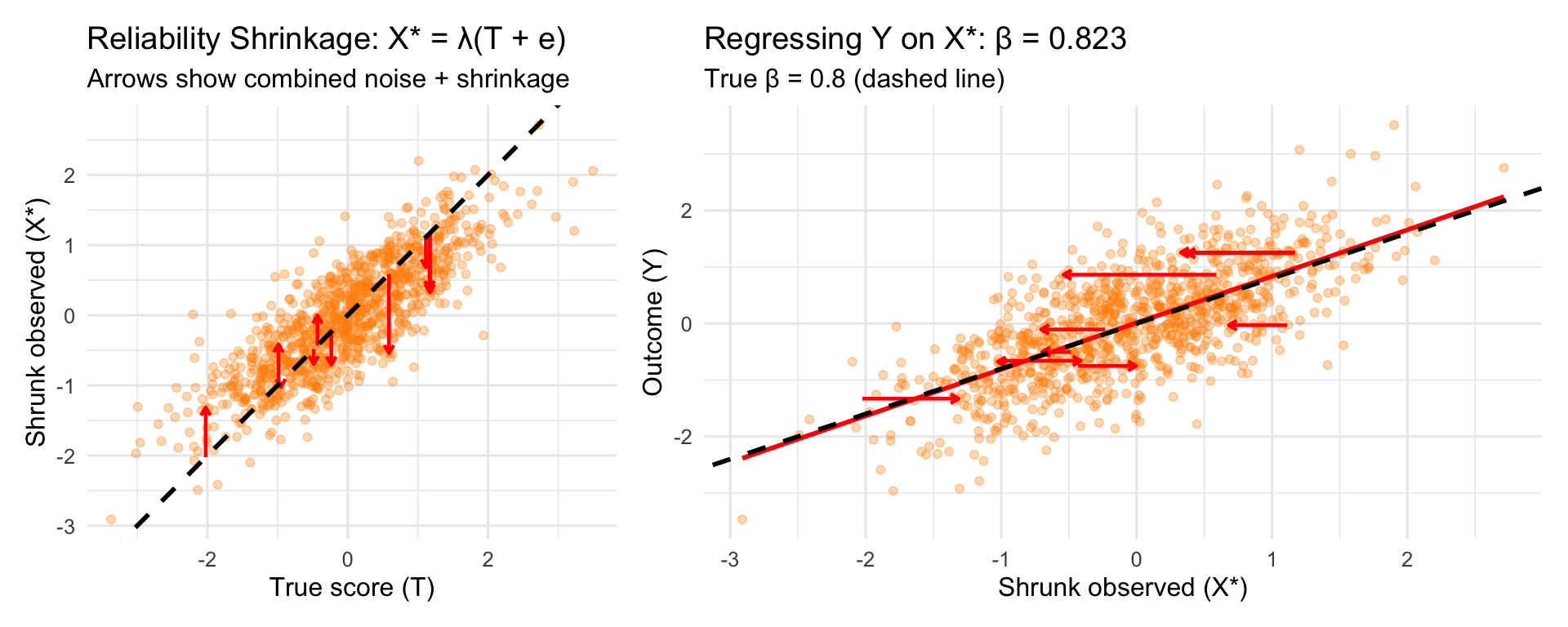
It works! \(\hat{\beta} =\) 0.826 \(\approx\) 0.8. In the univariate case that is.
Show numbers
Show code
# Simulation function for reliability shrinkage
sim_shrinkage <- function(n = 3000, beta_true = 0.8, error_sd = 0.7) {
  T_true <- rnorm(n)
  epsilon <- rnorm(n, sd = 0.5)
  Y <- beta_true * T_true + epsilon
  X_raw <- T_true + rnorm(n, sd = error_sd)
  reliability <- var(T_true) / var(X_raw)
  X_shrunk <- reliability * X_raw + (1 - reliability) * mean(X_raw)
  fit <- lm(Y ~ X_shrunk)
  ci <- confint(fit)[2, ]
  list(estimate = coef(fit)[2], ci_lower = ci[1], ci_upper = ci[2])
}

set.seed(123)
coverage_shrinkage <- run_coverage_sim(sim_shrinkage, n_sims = 1000, true_beta = beta_true)
cat("Coverage (95% CI includes true β):", round(coverage_shrinkage$coverage * 100, 1), "%\n")
Coverage (95% CI includes true β): 94.4 %Mean estimate: 0.8 Bias: 0 The coverage is close to nominal (94.4%) in the univariate case.
Mathematically, the shrinkage reduces \(\text{Var}(X)\) by exactly the factor needed to offset the attenuation. It’s algebraically equivalent to dividing the attenuated slope by the reliability.
Visually, it’s the same as above.
Multivariate case
So why don’t we do this all the time? The problem emerges in the multivariate case (and presumably in many other cases). Let’s see:
Show code
set.seed(456)
n <- 2000
beta1 <- 0.6
beta2 <- 0.4

# Correlated true scores
rho_T <- 0.5
T1 <- rnorm(n)
T2 <- rho_T * T1 + sqrt(1 - rho_T^2) * rnorm(n)

Y_multi <- beta1 * T1 + beta2 * T2 + rnorm(n, sd = 0.5)

# Classical error
e1 <- rnorm(n, sd = 0.7)
e2 <- rnorm(n, sd = 0.7)
X1_classical <- T1 + e1
X2_classical <- T2 + e2

# Berkson error
z_error_sd <- 1
Z1 <- T1 + rnorm(n, sd = z_error_sd)
Z2 <- T2 + rnorm(n, sd = z_error_sd)

# Univariate Berkson (theoretical coefficients)
# Slope = Var(T) / Var(Z) = 1 / (1 + 1^2) = 0.5
slope_uni <- 1 / (1 + z_error_sd^2)
X1_berkson <- slope_uni * Z1
X2_berkson <- slope_uni * Z2

# Mutual adjustment Berkson (theoretical coefficients)
# Calculate population regression coefficients
Sigma_T <- matrix(c(1, rho_T, rho_T, 1), 2, 2)
Sigma_Z <- Sigma_T + diag(z_error_sd^2, 2)
Sigma_TZ <- Sigma_T
Coef_mat <- Sigma_TZ %*% solve(Sigma_Z)

X_berkson_adj_mat <- cbind(Z1, Z2) %*% t(Coef_mat)
X1_berkson_adj <- X_berkson_adj_mat[, 1]
X2_berkson_adj <- X_berkson_adj_mat[, 2]

# Outcome for Berkson case (same true scores, same betas)
Y_berkson_multi <- beta1 * T1 + beta2 * T2 + rnorm(n, sd = 0.5)

# Reliability shrinkage (Kelley formula)
rel1 <- var(T1) / var(X1_classical)
rel2 <- var(T2) / var(X2_classical)
X1_shrunk <- rel1 * X1_classical + (1 - rel1) * mean(X1_classical)
X2_shrunk <- rel2 * X2_classical + (1 - rel2) * mean(X2_classical)

# Fit models
fit_oracle <- lm(Y_multi ~ T1 + T2)
fit_classical <- lm(Y_multi ~ X1_classical + X2_classical)
fit_berkson <- lm(Y_berkson_multi ~ X1_berkson + X2_berkson)
fit_berkson_adj <- lm(Y_berkson_multi ~ X1_berkson_adj + X2_berkson_adj)
fit_shrunk <- lm(Y_multi ~ X1_shrunk + X2_shrunk)

results <- data.frame(
  Method = c("Oracle (true T)", "Classical error", "Berkson (separate Z)",
             "Berkson (mutual adj.)", "Reliability shrinkage"),
  beta1 = c(coef(fit_oracle)[2], coef(fit_classical)[2],
            coef(fit_berkson)[2], coef(fit_berkson_adj)[2], coef(fit_shrunk)[2]),
  beta2 = c(coef(fit_oracle)[3], coef(fit_classical)[3],
            coef(fit_berkson)[3], coef(fit_berkson_adj)[3], coef(fit_shrunk)[3])
)

knitr::kable(results, digits = 3,
caption = "Multivariate regression: True β1 = 0.6, β2 = 0.4")| Method | beta1 | beta2 | |
|---|---|---|---|
| T1 | Oracle (true T) | 0.600 | 0.401 |
| X1_classical | Classical error | 0.423 | 0.329 |
| X1_berkson | Berkson (separate Z) | 0.701 | 0.515 |
| X1_berkson_adj | Berkson (mutual adj.) | 0.646 | 0.367 |
| X1_shrunk | Reliability shrinkage | 0.664 | 0.485 |
The “Berkson (mutual adj.)” row shows what happens when we predict T1 and T2 using both Z1 and Z2 using theoretical population coefficients (equivalent to a large training set).
Show code
# Simulation function for multivariate coverage
sim_multivariate <- function(n = 2000, beta1 = 0.6, beta2 = 0.4, rho_T = 0.5) {
  T1 <- rnorm(n)
  T2 <- rho_T * T1 + sqrt(1 - rho_T^2) * rnorm(n)
  epsilon <- rnorm(n, sd = 0.5)
  Y <- beta1 * T1 + beta2 * T2 + epsilon

  # Classical error
  X1_classical <- T1 + rnorm(n, sd = 0.7)
  X2_classical <- T2 + rnorm(n, sd = 0.7)
  fit_classical <- lm(Y ~ X1_classical + X2_classical)
  ci_classical <- confint(fit_classical)

  # Berkson error setup
  z_error_sd <- 1
  Z1 <- T1 + rnorm(n, sd = z_error_sd)
  Z2 <- T2 + rnorm(n, sd = z_error_sd)

  # Univariate Berkson (theoretical)
  slope_uni <- 1 / (1 + z_error_sd^2)
  X1_berkson <- slope_uni * Z1
  X2_berkson <- slope_uni * Z2
  fit_berkson <- lm(Y ~ X1_berkson + X2_berkson)
  ci_berkson <- confint(fit_berkson)

  # Mutual adjustment Berkson (theoretical)
  Sigma_T <- matrix(c(1, rho_T, rho_T, 1), 2, 2)
  Sigma_Z <- Sigma_T + diag(z_error_sd^2, 2)
  Coef_mat <- Sigma_T %*% solve(Sigma_Z)

  X_berkson_adj_mat <- cbind(Z1, Z2) %*% t(Coef_mat)
  X1_berkson_adj <- X_berkson_adj_mat[, 1]
  X2_berkson_adj <- X_berkson_adj_mat[, 2]

  fit_berkson_adj <- lm(Y ~ X1_berkson_adj + X2_berkson_adj)
  ci_berkson_adj <- confint(fit_berkson_adj)

  # Reliability shrinkage
  rel1 <- var(T1) / var(X1_classical)
  rel2 <- var(T2) / var(X2_classical)
  X1_shrunk <- rel1 * X1_classical + (1 - rel1) * mean(X1_classical)
  X2_shrunk <- rel2 * X2_classical + (1 - rel2) * mean(X2_classical)
  fit_shrunk <- lm(Y ~ X1_shrunk + X2_shrunk)
  ci_shrunk <- confint(fit_shrunk)

  list(
    classical_b1 = coef(fit_classical)[2],
    classical_b1_covers = ci_classical[2, 1] <= beta1 & ci_classical[2, 2] >= beta1,
    classical_b2 = coef(fit_classical)[3],
    classical_b2_covers = ci_classical[3, 1] <= beta2 & ci_classical[3, 2] >= beta2,

    berkson_b1 = coef(fit_berkson)[2],
    berkson_b1_covers = ci_berkson[2, 1] <= beta1 & ci_berkson[2, 2] >= beta1,
    berkson_b2 = coef(fit_berkson)[3],
    berkson_b2_covers = ci_berkson[3, 1] <= beta2 & ci_berkson[3, 2] >= beta2,

    berkson_adj_b1 = coef(fit_berkson_adj)[2],
    berkson_adj_b1_covers = ci_berkson_adj[2, 1] <= beta1 & ci_berkson_adj[2, 2] >= beta1,
    berkson_adj_b2 = coef(fit_berkson_adj)[3],
    berkson_adj_b2_covers = ci_berkson_adj[3, 1] <= beta2 & ci_berkson_adj[3, 2] >= beta2,

    shrunk_b1 = coef(fit_shrunk)[2],
    shrunk_b1_covers = ci_shrunk[2, 1] <= beta1 & ci_shrunk[2, 2] >= beta1,
    shrunk_b2 = coef(fit_shrunk)[3],
    shrunk_b2_covers = ci_shrunk[3, 1] <= beta2 & ci_shrunk[3, 2] >= beta2
  )
}

set.seed(123)
n_sims <- 1000
multi_results <- replicate(n_sims, sim_multivariate(), simplify = FALSE)

# Summarize coverage
coverage_summary <- data.frame(
  Method = c("Classical error", "Berkson (separate Z)", "Berkson (mutual adj.)", "Reliability shrinkage"),
  `Mean β1` = c(
    mean(sapply(multi_results, `[[`, "classical_b1")),
    mean(sapply(multi_results, `[[`, "berkson_b1")),
    mean(sapply(multi_results, `[[`, "berkson_adj_b1")),
    mean(sapply(multi_results, `[[`, "shrunk_b1"))
  ),
  `Coverage β1` = c(
    mean(sapply(multi_results, `[[`, "classical_b1_covers")),
    mean(sapply(multi_results, `[[`, "berkson_b1_covers")),
    mean(sapply(multi_results, `[[`, "berkson_adj_b1_covers")),
    mean(sapply(multi_results, `[[`, "shrunk_b1_covers"))
  ),
  `Mean β2` = c(
    mean(sapply(multi_results, `[[`, "classical_b2")),
    mean(sapply(multi_results, `[[`, "berkson_b2")),
    mean(sapply(multi_results, `[[`, "berkson_adj_b2")),
    mean(sapply(multi_results, `[[`, "shrunk_b2"))
  ),
  `Coverage β2` = c(
    mean(sapply(multi_results, `[[`, "classical_b2_covers")),
    mean(sapply(multi_results, `[[`, "berkson_b2_covers")),
    mean(sapply(multi_results, `[[`, "berkson_adj_b2_covers")),
    mean(sapply(multi_results, `[[`, "shrunk_b2_covers"))
  ),
  check.names = FALSE
)

knitr::kable(coverage_summary, digits = 3,
caption = "Multivariate coverage (1000 simulations): True β1 = 0.6, β2 = 0.4")| Method | Mean β1 | Coverage β1 | Mean β2 | Coverage β2 |
|---|---|---|---|---|
| Classical error | 0.428 | 0.000 | 0.327 | 0.001 |
| Berkson (separate Z) | 0.668 | 0.199 | 0.533 | 0.000 |
| Berkson (mutual adj.) | 0.601 | 0.951 | 0.400 | 0.951 |
| Reliability shrinkage | 0.638 | 0.501 | 0.486 | 0.010 |
Now we see the difference:
- Classical error: Both coefficients attenuated.
- Berkson (separate Z): Both coefficients are biased. Because \(T_1\) and \(T_2\) are correlated, \(Z_1\) contains information about \(T_2\) and \(Z_2\) about \(T_1\). By not mutually adjusting, we fail to ensure the error in \(X_1\) is orthogonal to \(X_2\). This is effectively a form of residual confounding.
- Berkson (mutual adj.): Both coefficients correct. By using all auxiliary information (\(Z_1, Z_2\)) to predict each true score, we ensure the prediction errors are orthogonal to all predictors. We could also achieve this by using a multivariate regression model on \(Y\) with \(Z_1\) and \(Z_2\) as predictors.
- Reliability shrinkage: Both coefficients inflated. The shrinkage approach fails in multivariate regression because it only corrects the variances, not the covariances. When predictors are correlated, you need to adjust the entire covariance matrix, which requires a proper errors-in-variables or SEM approach.
The coverage table above shows that:
- Not adjusting (Classical error) has poor coverage because estimates are biased.
- Berkson (separate Z) has poor coverage in the multivariate case because of the bias induced by the correlation between predictors.
- Berkson (mutual adj.) maintains nominal coverage.
- Reliability shrinkage has poor coverage because estimates are inflated.
A technical note on standard errors: You might wonder why we didn’t need to adjust the standard errors, given the “generated regressor” literature mentioned earlier. In these simulations, we used the theoretical population coefficients to generate the predictions. This corresponds to a scenario where you are using a high-quality pre-trained model (effectively “known” weights). In this case, standard OLS standard errors are correct because OLS automatically estimates the residual variance, which includes both the structural error \(\varepsilon\) and the Berkson error component. If the weights were estimated from a small training sample, you would indeed need to adjust the standard errors to account for the uncertainty in those weights.
Visual Summary
Show code
# Combine the plots from the three scenarios
(p1_classical + p2_classical) / (p1_berkson + p2_berkson) / (p1_shrink + p2_shrink)  +
  plot_layout(widths = c(1, 1.5))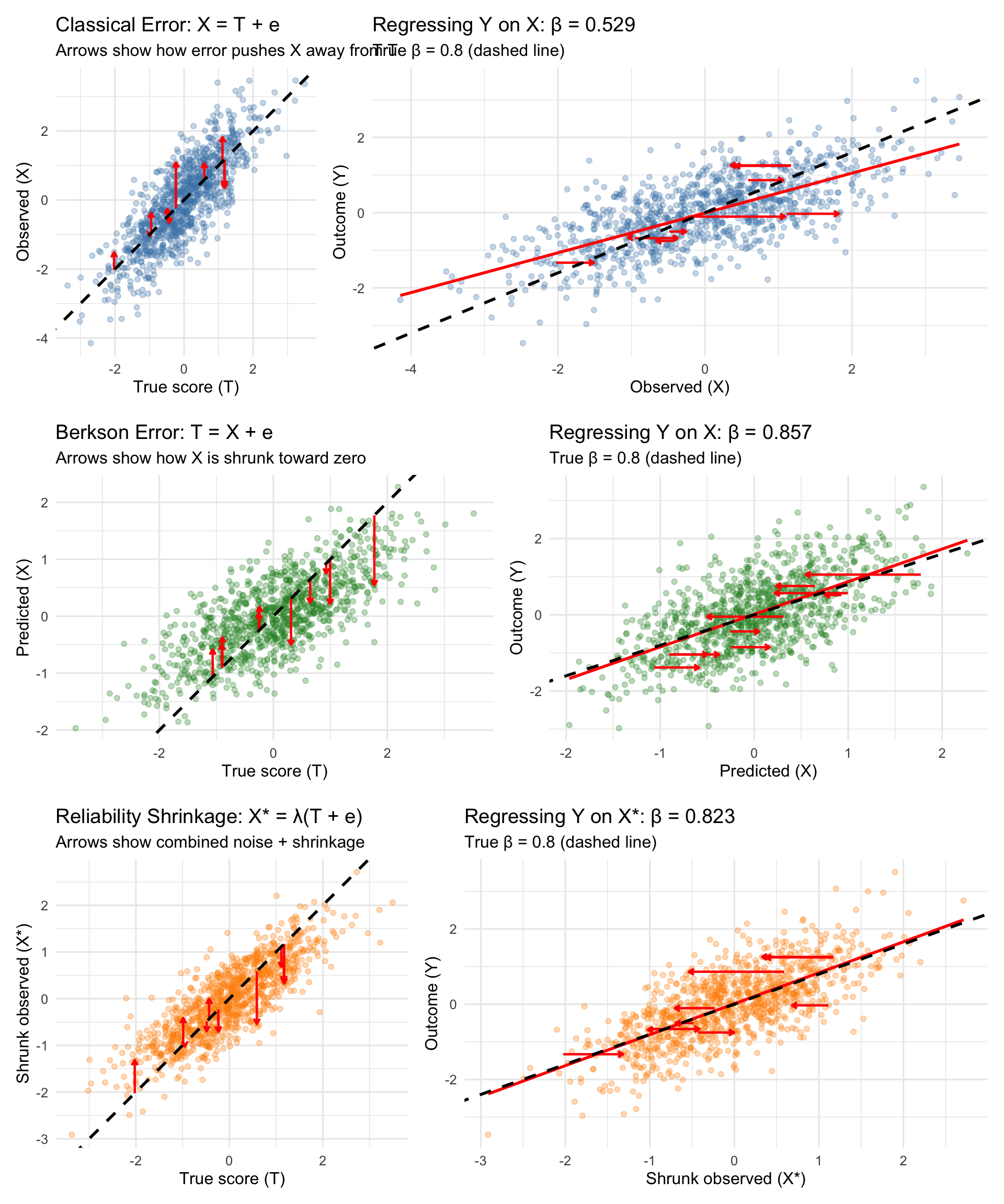
Tabular Summary
| Error Type | Structure | What is X? | Univariate bias | Multivariate bias | Coverage |
|---|---|---|---|---|---|
| Classical | X = T + e, e⊥T | Noisy measurement | Attenuated | Attenuated | Poor |
| Berkson (univariate) | T = X + e, e⊥X | Prediction/conditional expectation | None | Biased (if correlated) | Nominal |
| Berkson (mutual adj.) | T = X + e, e⊥X | Multivariate prediction | None | None | Nominal |
| Reliability shrinkage | X* = λ(T+e) | “Corrected” measurement | None | Inflated | Poor |
The key insight for here is that it depends on the error model, specifically whether the error is independent of the predictor you’re using.
- In classical error, the error is part of X, so it correlates with X and biases slopes (it’s independent of T though).
- In Berkson error, the error is independent of X by construction, so OLS works fine.
So, when you use predicted values (from regression, imputation, machine learning, etc.) as predictors, you have Berkson error. The predictions will be “shrunken” relative to the true values, but that’s fine. The slope will be correct, even the standard errors won’t be far off if your estimates are not too imprecise. You should not apply a classical-error correction with SEM/EIV, that would make things worse.
In econometrics, this problem is often discussed under the label “generated regressors” (e.g., Pagan, 1984). That literature focuses on the fact that while coefficients are consistent (if the generated regressor is a conditional expectation), the standard errors need adjustment because the regressor is estimated, not known.↩︎
Note that we use the theoretical population coefficients to generate the predictions here. If we used the sample coefficients (training and testing on the same data), we would artificially inflate the coverage because the prediction error would be orthogonal to the predictor in the sample (super-efficiency). In practice, using a pre-trained model corresponds to the theoretical coefficient case.↩︎