Re-analysis of OCMATE data to get reliability of change
Pre-process data
# Load packages
library(tidyr)
library(dplyr)
##
## Attaching package: 'dplyr'## The following objects are masked from 'package:stats':
##
## filter, lag## The following objects are masked from 'package:base':
##
## intersect, setdiff, setequal, unionlibrary(ggplot2)
library(lme4)## Loading required package: Matrix##
## Attaching package: 'Matrix'## The following object is masked from 'package:tidyr':
##
## expandlibrary(lmerTest)##
## Attaching package: 'lmerTest'## The following object is masked from 'package:lme4':
##
## lmer## The following object is masked from 'package:stats':
##
## steplibrary(knitr)
options(scipen=999)
knitr::opts_chunk$set(cache=TRUE)# calculate standard errors
se <- function(x, na.rm = FALSE) {
if (na.rm) {
the.SE <- sqrt(var(x,na.rm=TRUE)/length(na.omit(x)))
} else {
the.SE <- sqrt(var(x,na.rm=FALSE)/length(x))
}
return(the.SE)
}
# short summaries for lmerTest
mySummary<-function(lmer_summary) {
coefTable <- lmer_summary$coefficients %>%
round(3) %>%
as.data.frame() %>%
rownames_to_column()
if (ncol(coefTable)>5) {
coefTable <- coefTable %>%
mutate(
sig = ifelse(.[6]<.001, " * * * ",
ifelse(.[6]<.01, " * * ",
ifelse(.[6]<.05, " * ",
ifelse(.[6]<.10, "+", "")))))
}
return(list(lmer_summary$ngrps, kable(coefTable)))
}Load data
Data entered from all white, heterosexual women not using any form of hormonal contraceptives Each row is all data from a single session (i.e. oc_id:date)
- “oc_id” = ID of the subject
- “block” = testing block (1, 2 or 3)
- “block_N” = how many testing sessions completed in that block
- “age” = age (in years) of subject on day of testing
- “ethnicity” = ethnic group of subject (all white)
- “sexpref” = sexual preference of subject (all heterosexual)
- “date” = date of testing session
- “partner” = does subject currently have a romantic partner? (0 = no partner, 1 = yes partner)
- “block_partner” = all unique partner column values in the block (0 if never had partner, 1 if always had partner, otherwised mixed: e.g., 1,0)
- “behavior_soi” = behavior subscale of SOI-R
- “attitude_soi” = attitude subscale of SOI-R
- “desire_soi” = desire subscale of SOI-R
- “current_sexdrive”= current sex drive score
- “solitary_SDI” = solitary desire subscale of SDI-2
- “dyadic_SDI” = dyadic desire subscale of SDI-2
- “total_SDI” = total score on SDI-2
- “progesterone” = salivary progesterone for that session
- “estradiol” = salivary estradiol for that session
- “testosterone” = salivary testosterone for that session
- “cortisol” = salivary cortisol for that session
data_start <- read.csv("OCMATE_sexdrive_anon.csv", stringsAsFactors = F) Re-code variables
- partner.e = partnership status (no = -0.5, partner = +0.5, mixed = NA)
# wide to long format
# effect code partnership status (no = -0.5, partner = 0.5)

data_all <- data_start %>%
  gather(question, score, behavior_soi:total_SDI) %>%
  mutate(
    partner.e = ifelse(block_partner==0, -0.5, ifelse(block_partner==1, 0.5, NA)),
    prog = progesterone,
    estr = estradiol,
    test = testosterone,
    cort = cortisol
  )
Age
# mean age at start of testing
data_all %>%
  group_by(oc_id) %>%
  summarise(
    min_age = min(age, na.rm = TRUE)
  ) %>%
  ungroup() %>%
  group_by() %>%
  summarise(
    n = n(),
    mean_age = mean(min_age, na.rm = TRUE),
    sd_age = sd(min_age, na.rm = TRUE)
  ) %>% t()
## [,1]
## n 375
## mean_age Inf
## sd_age InfDescriptive Stats for Questionaires
data_all %>%
  group_by(question) %>%
  summarise(
    N_valid = sum(!is.na(score)),
    N_missing = sum(is.na(score)),
    mean_score = mean(score, na.rm = TRUE),
    sd_score = sd(score, na.rm = TRUE)
  )
## # A tibble: 7 x 5
## question N_valid N_missing mean_score sd_score
## <chr> <int> <int> <dbl> <dbl>
## 1 attitude_soi 2189 87 9.22 3.50
## 2 behavior_soi 2140 136 5.74 2.67
## 3 current_sexdrive 2145 131 3.77 1.56
## 4 desire_soi 2168 108 8.06 2.96
## 5 dyadic_SDI 2098 178 35.5 11.9
## 6 solitary_SDI 2099 177 8.63 6.46
## 7 total_SDI 2051 225 44.1 15.7The number of sessions completed per woman
data_all %>%
  group_by(oc_id) %>%
  summarise(
    sessions = n_distinct(date)
  ) %>%
  group_by(sessions) %>%
  summarise(
    n = n()
  ) %>%
  spread(sessions, n) %>%
  t()
## [,1]
## 1 15
## 2 9
## 3 5
## 4 9
## 5 233
## 6 1
## 7 1
## 8 2
## 9 2
## 10 98Exclude observations with missing estr, prog and test
## Exclude observations with EPT missing hormone values
sub_hormones_no_EPT <- data_all %>%
  filter(
    !is.na(prog) |
    !is.na(estr) |
    !is.na(test)
  )
Exclude subjects with only a single session in a block
This is necessary because you can’t calculate subject-centered means with only one data point.
check_single_session <- sub_hormones_no_EPT %>%
  group_by(oc_id, block) %>%
  summarise(sessions = n_distinct(date)) %>%
  ungroup() %>%
  filter(sessions == 1)

sub_hormones_multisession <- sub_hormones_no_EPT %>%
  anti_join(check_single_session, by=c('oc_id', 'block'))
Remove outlier hormone values
Remove below bottom sensitivity thresholds for assays (progesterone < 5, estrogen < 0.1), and remove outlier values (+/- 3SD from the mean)
sub_hormones_no_outliers <- sub_hormones_multisession %>%
  mutate(
    prog = ifelse(prog >= 5, prog, NA),
    estr = ifelse(estr >= 0.1, estr, NA),
    prog = if_else(prog>mean(prog, na.rm=TRUE) + 3*sd(prog, na.rm=TRUE) |
                  prog<mean(prog, na.rm=TRUE) - 3*sd(prog, na.rm=TRUE), NA_real_, prog),
    estr = ifelse(estr>mean(estr, na.rm=TRUE) + 3*sd(estr, na.rm=TRUE) |
                  estr<mean(estr, na.rm=TRUE) - 3*sd(estr, na.rm=TRUE), NA, estr),
    test = ifelse(test>mean(test, na.rm=TRUE) + 3*sd(test, na.rm=TRUE) |
                  test<mean(test, na.rm=TRUE) - 3*sd(test, na.rm=TRUE), NA, test),
    cort = ifelse(cort>mean(cort, na.rm=TRUE) + 3*sd(cort, na.rm=TRUE) |
                  cort<mean(cort, na.rm=TRUE) - 3*sd(cort, na.rm=TRUE), NA, cort)
  )
qplot(sub_hormones_no_outliers$prog)
## `stat_bin()` using `bins = 30`. Pick better value with `binwidth`.## Warning: Removed 287 rows containing non-finite values (stat_bin).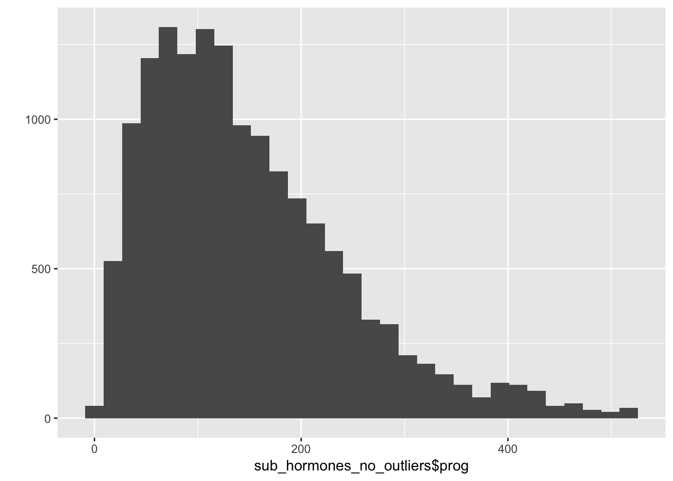
# how many included?
check_hormone_exclusions <- sub_hormones_no_outliers %>%
  group_by(oc_id, date) %>%
  summarise(
    e = is.na(mean(estr)),
    p = is.na(mean(prog)),
    t = is.na(mean(test)),
    c = is.na(mean(cort))
  ) %>%
  ungroup() %>%
  select(e:c) %>%
  gather('hormone','na', e:c) %>%
  group_by(hormone) %>%
  summarise(
    'valid' = n() - sum(na),
    'excluded' = sum(na)
  ) %>%
  arrange(hormone)

kable(check_hormone_exclusions)| hormone | valid | excluded |
|---|---|---|
| c | 2155 | 11 |
| e | 2146 | 20 |
| p | 2125 | 41 |
| t | 2143 | 23 |
  check_hormone_exclusions %>%
    group_by() %>%
    summarise(
      total_hormone_samples_valid = sum(valid),
      total_hormone_samples_excluded = sum(excluded)
    ) %>% gather("stat", "value", 1:length(.))
## # A tibble: 2 x 2
## stat value
## <chr> <int>
## 1 total_hormone_samples_valid 8569
## 2 total_hormone_samples_excluded 95Subject-mean-centre hormones
Divide results by a constant to put all hormones on ~ -0.5 to +0.5 scale
# subject-mean-centre hormones
# and divide by a constant to put all hormones on ~ -0.5 to +0.5 scale

data_hormones <- sub_hormones_no_outliers %>%
group_by(oc_id) %>%
  mutate(prog.s = (prog-mean(prog, na.rm=TRUE))/400,
         estr.s = (estr-mean(estr, na.rm=TRUE))/5,
         test.s = (test-mean(test, na.rm=TRUE))/100,
         cort.s = (cort-mean(cort, na.rm=TRUE))/0.5,
         ep_ratio.s = ((estr/prog)-mean(estr/prog, na.rm=TRUE))/0.075) %>%
  ungroup() %>%
  as.data.frame()

data_hormones %>%
  group_by(oc_id, date, prog.s, estr.s, test.s, cort.s, ep_ratio.s) %>%
  summarise(n = n()) %>%
  ungroup() %>%
  gather("hormone", "value", prog.s:ep_ratio.s) %>%
  ggplot(aes(value, colour=hormone)) +
  geom_density(alpha=.5) +
  scale_x_continuous(limits = c(-1,1))
## Warning: Removed 200 rows containing non-finite values (stat_density).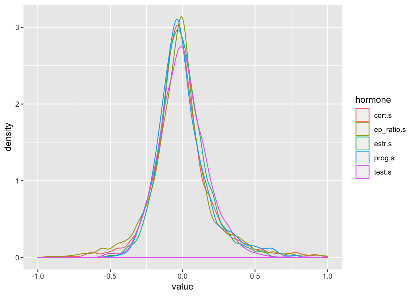
Mean Hormone Levels
data_hormones %>%
  group_by(oc_id, date, prog, estr, test, cort) %>%
  summarise(n = n()) %>%
  ungroup() %>%
  group_by() %>%
  summarise(
      mean_prog = mean(prog, na.rm = TRUE),
      sd_prog =   sd(prog, na.rm = TRUE),
      se_prog =   se(prog, na.rm = TRUE),
      mean_estr = mean(estr, na.rm = TRUE),
      sd_estr =   sd(estr, na.rm = TRUE),
      se_estr =   se(estr, na.rm = TRUE),
      mean_test = mean(test, na.rm = TRUE),
      sd_test =   sd(test, na.rm = TRUE),
      se_test =   se(test, na.rm = TRUE),
      mean_cort = mean(cort, na.rm = TRUE),
      sd_cort =   sd(cort, na.rm = TRUE),
      se_cort =   se(cort, na.rm = TRUE)
  ) %>% gather("stat", "value", 1:length(.)) %>%
    mutate(value = round(value, 4)) %>%
    separate(stat, c("stat", "hormone")) %>%
    spread(stat, value)
## # A tibble: 4 x 4
## hormone mean sd se
## <chr> <dbl> <dbl> <dbl>
## 1 cort 0.229 0.164 0.0035
## 2 estr 3.30 1.27 0.0275
## 3 prog 149. 96.2 2.09
## 4 test 87.6 27.2 0.587Partnership
Exclude blocks with partner inconsistently reported and women who change partnership status between blocks, only for analyses considering partnership status
data_hormones_partner <- data_hormones %>%
  filter(block_partner == "0" | block_partner =="1") %>%
  group_by(oc_id) %>%
  mutate(pchange = mean(partner.e)) %>%
  ungroup() %>%
  filter(pchange %in% c(-.5, .5)) %>%
  select(-pchange)
Multilevel Reliability / Generalizability Analyses
library(psych)
data_wide = data_hormones %>% select(oc_id, date, block, estr, prog, test, cort) %>% unique()
data_wide <- data_wide %>% group_by(oc_id) %>%
arrange(oc_id, date) %>%
mutate(timepoint = row_number()) %>%
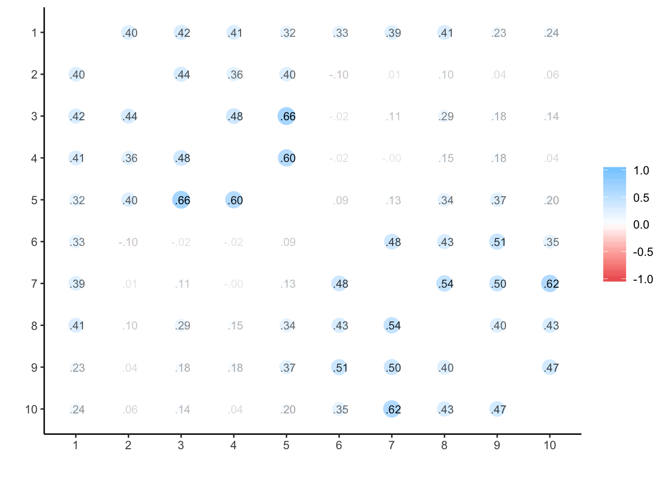
ungroup() %>% as.data.frame()Estradiol
multilevel.reliability(data_wide %>% select(oc_id, date, estr), "oc_id", "date", 3, aov = F)## Warning in cov2cor(C): diag(.) had 0 or NA entries; non-finite result is
## doubtful##
## Multilevel Generalizability analysis
## Call: multilevel.reliability(x = data_wide %>% select(oc_id, date,
## estr), grp = "oc_id", Time = "date", items = 3, aov = F)
##
## The data had 352 observations taken over 306 time intervals for 1 items.
##
## Alternative estimates of reliability based upon Generalizability theory
##
## RkRn = 1 Generalizability of between person differences averaged over time (time nested within people)
## Rcn = 0.83 Generalizability of within person variations averaged over items (time nested within people)
## The nested components of variance estimated from lme are:
## Variance Percent
## id 0.92 0.548
## id(time) 0.63 0.377
## residual 0.13 0.075
## total 1.68 1.000
##
## To see the ANOVA and alpha by subject, use the short = FALSE option.
## To see the summaries of the ICCs by subject and time, use all=TRUE
## To see specific objects select from the following list:
## ANOVA s.lmer s.lme alpha summary.by.person summary.by.time ICC.by.person ICC.by.time lmer long Calldata_wide %>%
select(oc_id, timepoint, estr) %>%
spread(timepoint, estr) %>%
select(-oc_id) %>%
cor(use='na.or.complete') %>%
corrr::rplot(print_cor = T)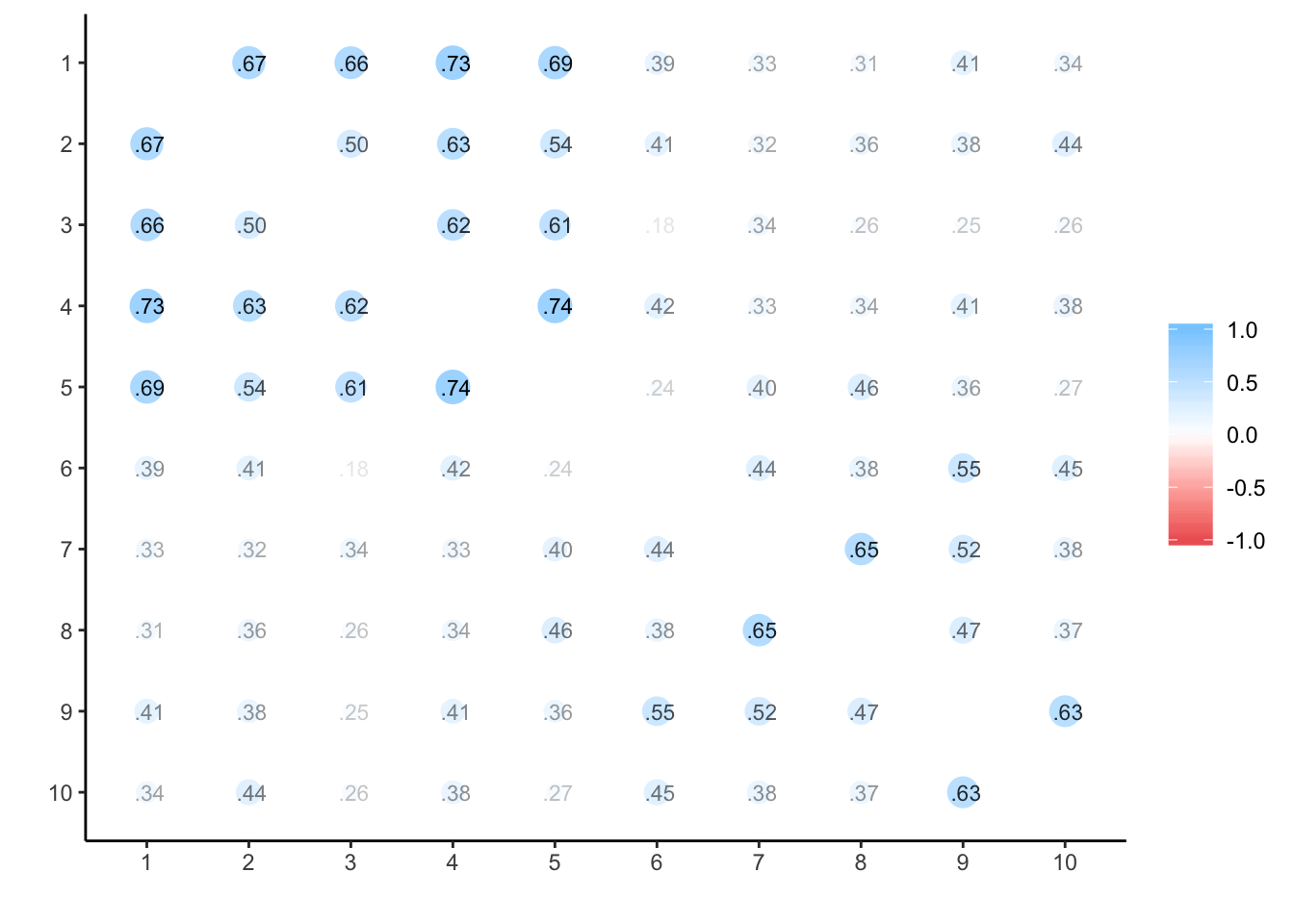
Progesterone
multilevel.reliability(data_wide %>% select(oc_id, date, prog), "oc_id", "date", 3, aov = F)##
## Multilevel Generalizability analysis
## Call: multilevel.reliability(x = data_wide %>% select(oc_id, date,
## prog), grp = "oc_id", Time = "date", items = 3, aov = F)
##
## The data had 352 observations taken over 306 time intervals for 1 items.
##
## Alternative estimates of reliability based upon Generalizability theory
##
## RkRn = 0.99 Generalizability of between person differences averaged over time (time nested within people)
## Rcn = 0.86 Generalizability of within person variations averaged over items (time nested within people)
## The nested components of variance estimated from lme are:
## Variance Percent
## id 3014 0.324
## id(time) 5392 0.579
## residual 899 0.097
## total 9305 1.000
##
## To see the ANOVA and alpha by subject, use the short = FALSE option.
## To see the summaries of the ICCs by subject and time, use all=TRUE
## To see specific objects select from the following list:
## ANOVA s.lmer s.lme alpha summary.by.person summary.by.time ICC.by.person ICC.by.time lmer long Calldata_wide %>%
select(oc_id, timepoint, prog) %>%
spread(timepoint, prog) %>%
select(-oc_id) %>%
cor(use='na.or.complete') %>%
corrr::rplot(print_cor = T)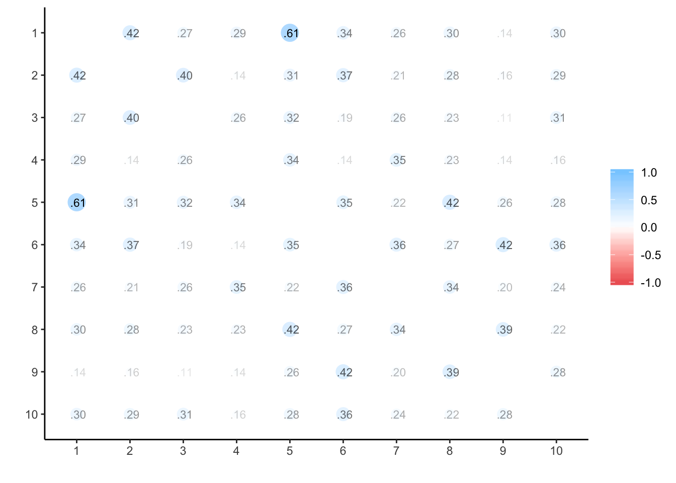
Testosterone
multilevel.reliability(data_wide %>% select(oc_id, date, test), "oc_id", "date", 3, aov = F)## Warning in cov2cor(C): diag(.) had 0 or NA entries; non-finite result is
## doubtful##
## Multilevel Generalizability analysis
## Call: multilevel.reliability(x = data_wide %>% select(oc_id, date,
## test), grp = "oc_id", Time = "date", items = 3, aov = F)
##
## The data had 352 observations taken over 306 time intervals for 1 items.
##
## Alternative estimates of reliability based upon Generalizability theory
##
## RkRn = 1 Generalizability of between person differences averaged over time (time nested within people)
## Rcn = 0.83 Generalizability of within person variations averaged over items (time nested within people)
## The nested components of variance estimated from lme are:
## Variance Percent
## id 432 0.573
## id(time) 268 0.355
## residual 55 0.072
## total 755 1.000
##
## To see the ANOVA and alpha by subject, use the short = FALSE option.
## To see the summaries of the ICCs by subject and time, use all=TRUE
## To see specific objects select from the following list:
## ANOVA s.lmer s.lme alpha summary.by.person summary.by.time ICC.by.person ICC.by.time lmer long Calldata_wide %>%
select(oc_id, timepoint, test) %>%
spread(timepoint, test) %>%
select(-oc_id) %>%
cor(use='na.or.complete') %>%
corrr::rplot(print_cor = T)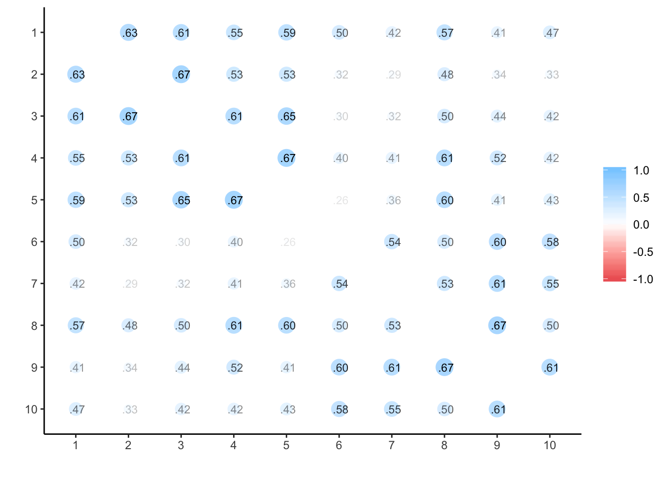
# data_wide %>% select(oc_id, date, test) %>% group_by(oc_id) %>%
# arrange(oc_id, date) %>%
# mutate(
# date = as.Date(date),
# time_since_start = round(as.numeric(date - min(date)))) %>%
# ungroup() %>%
# spread(time_since_start, test) %>%
# select(-oc_id, -date) %>%
# cor(use='na.or.complete') %>%
# corrr::rplot(print_cor = T)Cortisol
multilevel.reliability(data_wide %>% select(oc_id, date, cort), "oc_id", "date", 3, aov = F)## Warning in cov2cor(C): diag(.) had 0 or NA entries; non-finite result is
## doubtful
## Warning in cov2cor(C): diag(.) had 0 or NA entries; non-finite result is
## doubtful
##
## Multilevel Generalizability analysis
## Call: multilevel.reliability(x = data_wide %>% select(oc_id, date,
## cort), grp = "oc_id", Time = "date", items = 3, aov = F)
##
## The data had 352 observations taken over 306 time intervals for 1 items.
##
## Alternative estimates of reliability based upon Generalizability theory
##
## RkRn = 1 Generalizability of between person differences averaged over time (time nested within people)
## Rcn = 0.85 Generalizability of within person variations averaged over items (time nested within people)
## The nested components of variance estimated from lme are:
## Variance Percent
## id 0.0123 0.432
## id(time) 0.0137 0.481
## residual 0.0025 0.087
## total 0.0285 1.000
##
## To see the ANOVA and alpha by subject, use the short = FALSE option.
## To see the summaries of the ICCs by subject and time, use all=TRUE
## To see specific objects select from the following list:
## ANOVA s.lmer s.lme alpha summary.by.person summary.by.time ICC.by.person ICC.by.time lmer long Calldata_wide %>%
select(oc_id, timepoint, cort) %>%
spread(timepoint, cort) %>%
select(-oc_id) %>%
cor(use='na.or.complete') %>%
corrr::rplot(print_cor = T)