Preregistered ovulatory shift analyses
Cycling women (not on hormonal birth control)
Women on hormonal birth control
Analyses as preregistered on the Open Science Framework on March 19, 2014.
Load data
library(knitr)
opts_chunk$set(cache = F, warning = T, message = F, error = T)
source("0_helpers.R")
load("full_data.rdata")
diary$included = diary$included_lax
diary = diary %>%
  mutate(
  cohabitation = factor(cohabitation),
  partner_st_vs_lt = partner_attractiveness_shortterm - partner_attractiveness_longterm
)
diary$fertile = diary$fertile_narrow
opts_chunk$set(warning = T, fig.height = 7, fig.width = 7)
diary2 = diary %>% mutate(fertile = fertile_broad)
broad_models = models = list()
do_model = function(model, diary) {
outcome = names(model@frame)[1]
model = calculate_effects(model)
options = list(fig.path = paste0(knitr::opts_chunk$get("fig.path"), outcome, "-"),
cache.path = paste0(knitr::opts_chunk$get("cache.path"), outcome, "-"))
asis_knit_child("_pre_reg_model.Rmd", options = options)
}
do_moderators = function(model, diary) {
asis_knit_child("_pre_reg_moderators.Rmd")
}Preregistered hypotheses
The following hypotheses were registered on the Open Science Framework on the day that data collection began. We have reworded and reorganised them slightly for space and clarity.
- Ovulatory cycle shifts (increases during fertile window among naturally cycling women in a heterosexual relationship, but not for hormonal contraception users) in
- female extra-pair desire and behaviour
- female in-pair sexual desire
- having and initiating in-pair sexual intercourse (if circumstances allowed, e.g. partner was close by)
- subjective feelings of attractiveness
- choice of clothing (on the dimensions “sexy”, “figure-hugging”, “seductive”)
- reported male partner mate retention strategies
- narcissism on both dimensions of the NARC (admiration and rivalry)
- Moderation or shift hypotheses: The ovulatory increase in women’s extra-pair desires and reported male mate retention behaviour is strongest (and the in-pair desire increase is weakest) for women who perceive their partners
- as low in sexual and physical attractiveness
- as low in sexual attractiveness relative to long-term partner attractiveness
- as less attractive in relation to themselves
- Predicted ovulatory shifts are larger than, and independent of, potential ovulatory shifts in self-esteem
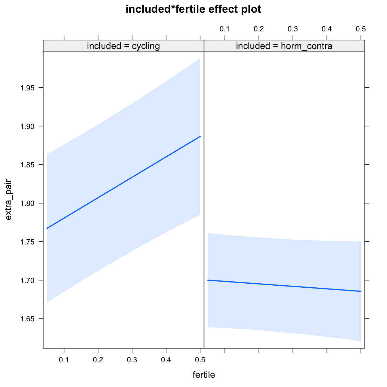
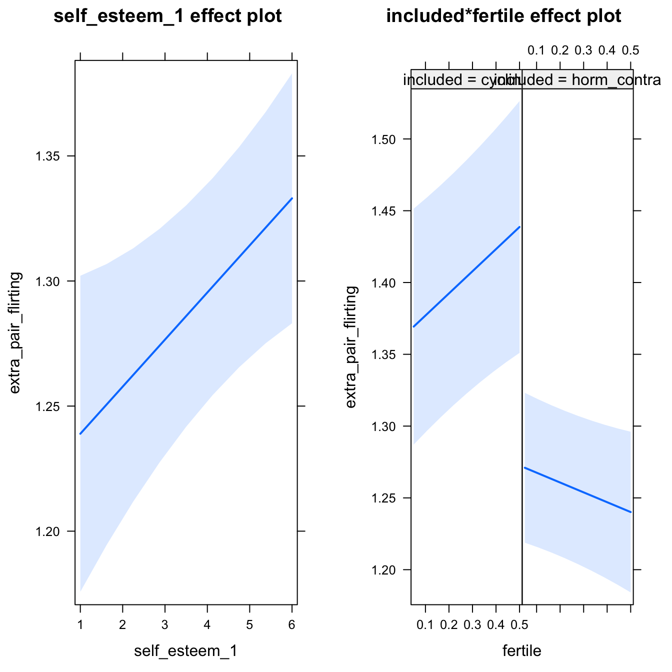
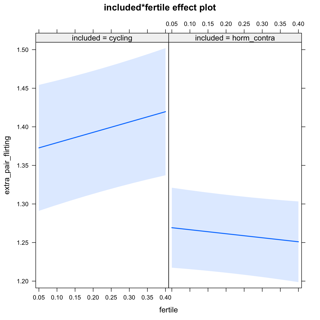
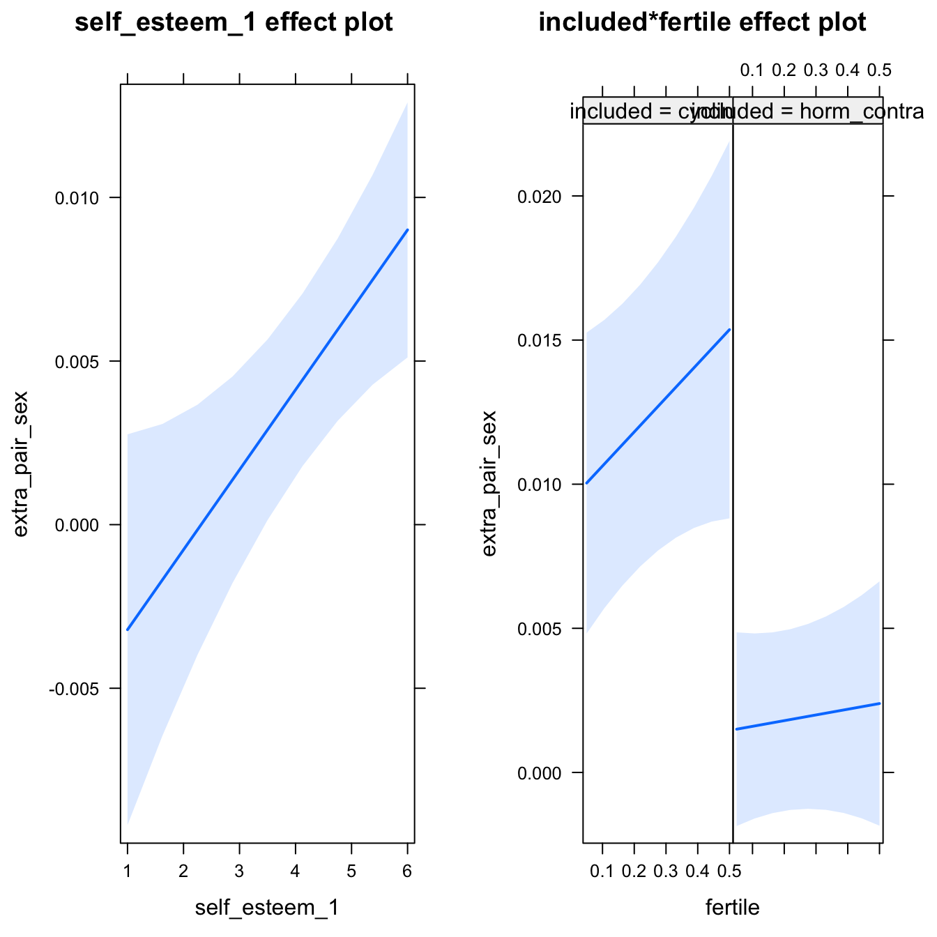
H1.1. Extra-pair
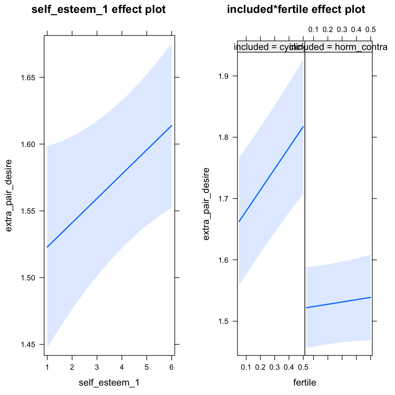
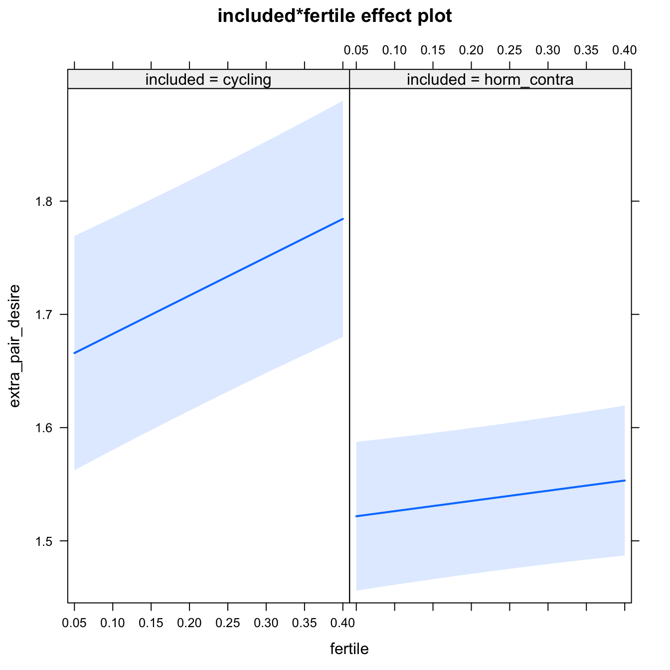
models$extra_pair = lmer(extra_pair ~ included * fertile + ( 1 | person), data = diary)
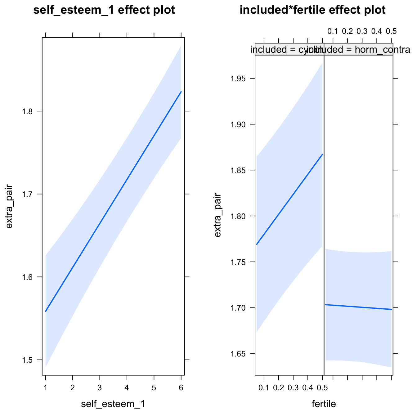
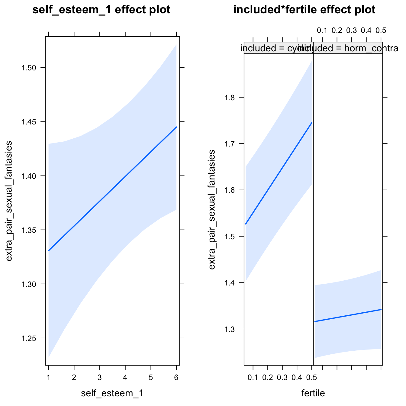
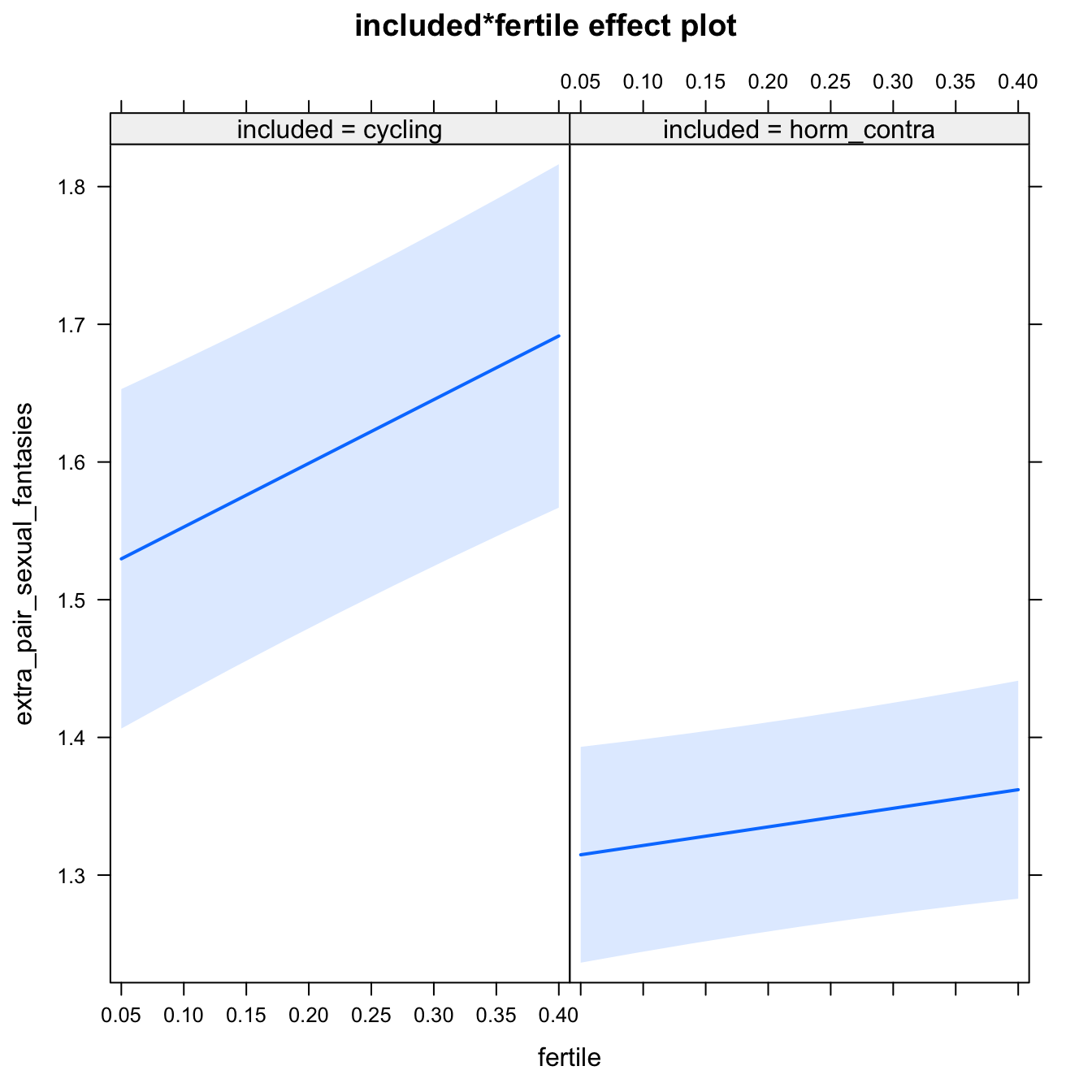
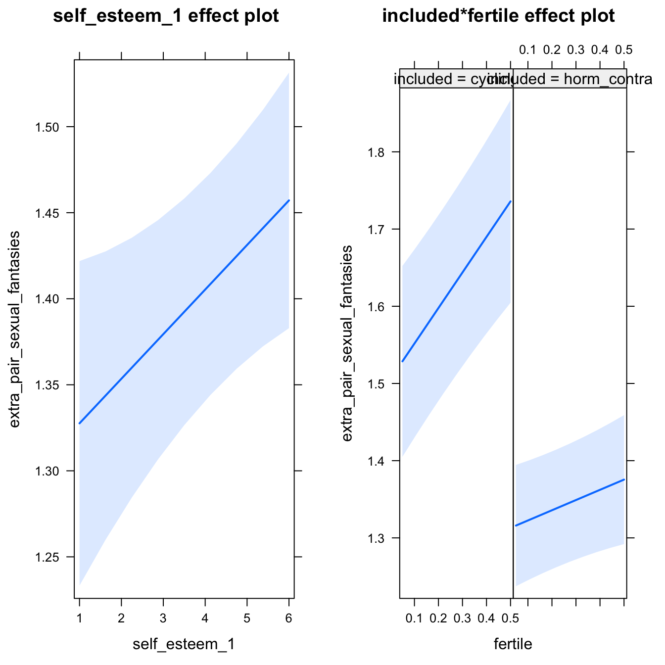
do_model(models$extra_pair, diary)Narrow window
model %>%
  print_summary() %>%
  plot_all_effects()
Linear mixed model fit by REML. t-tests use Satterthwaite's method ['lmerModLmerTest']
Formula: extra_pair ~ included * fertile + (1 | person)
Data: diary
REML criterion at convergence: 11341
Scaled residuals:
Min 1Q Median 3Q Max
-4.573 -0.546 -0.145 0.413 7.678
Random effects:
Groups Name Variance Std.Dev.
person (Intercept) 0.305 0.553
Residual 0.282 0.531
Number of obs: 6378, groups: person, 493
Fixed effects:
Estimate Std. Error df t value Pr(>|t|)
(Intercept) 1.7541 0.0497 537.2116 35.32 < 2e-16 ***
includedhorm_contra -0.0524 0.0588 539.7185 -0.89 0.37
fertile 0.2650 0.0594 5934.3721 4.46 0.0000084 ***
includedhorm_contra:fertile -0.2972 0.0712 5937.8105 -4.18 0.0000301 ***
---
Signif. codes: 0 '***' 0.001 '**' 0.01 '*' 0.05 '.' 0.1 ' ' 1
Correlation of Fixed Effects:
(Intr) incld_ fertil
inclddhrm_c -0.844
fertile -0.225 0.190
inclddhrm_: 0.188 -0.228 -0.835
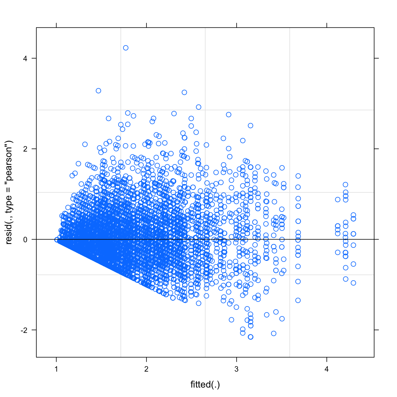
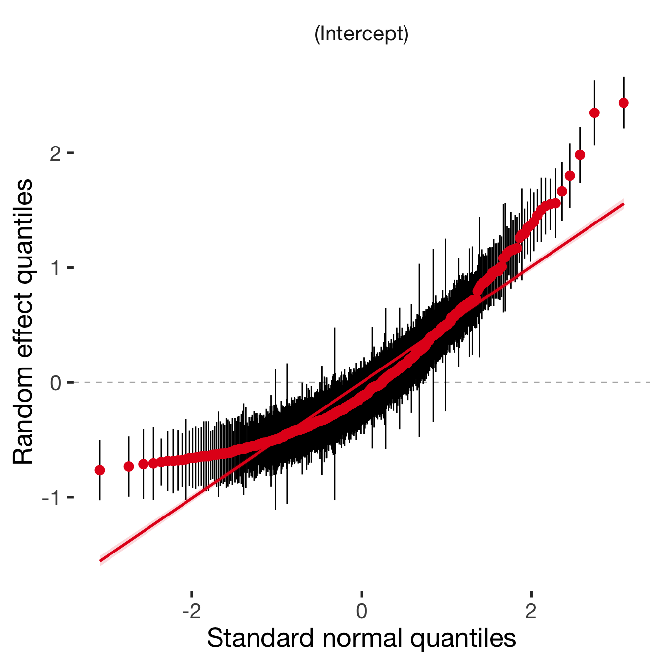
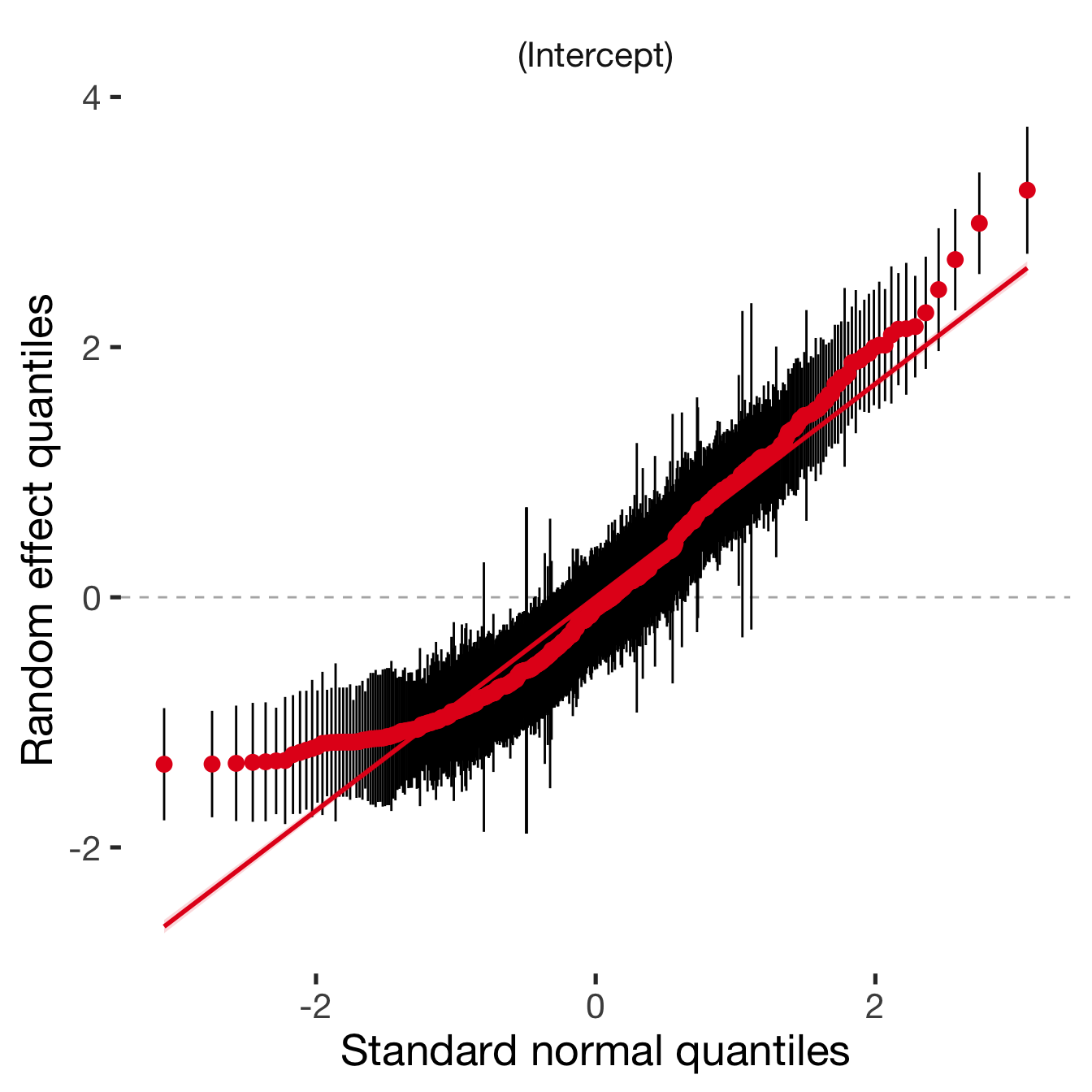
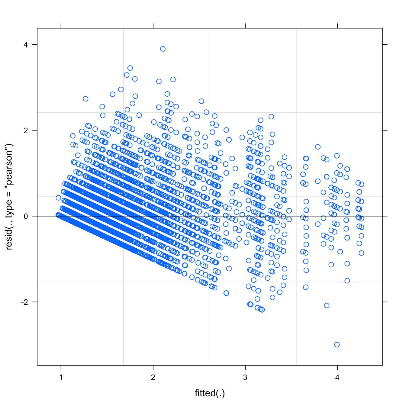
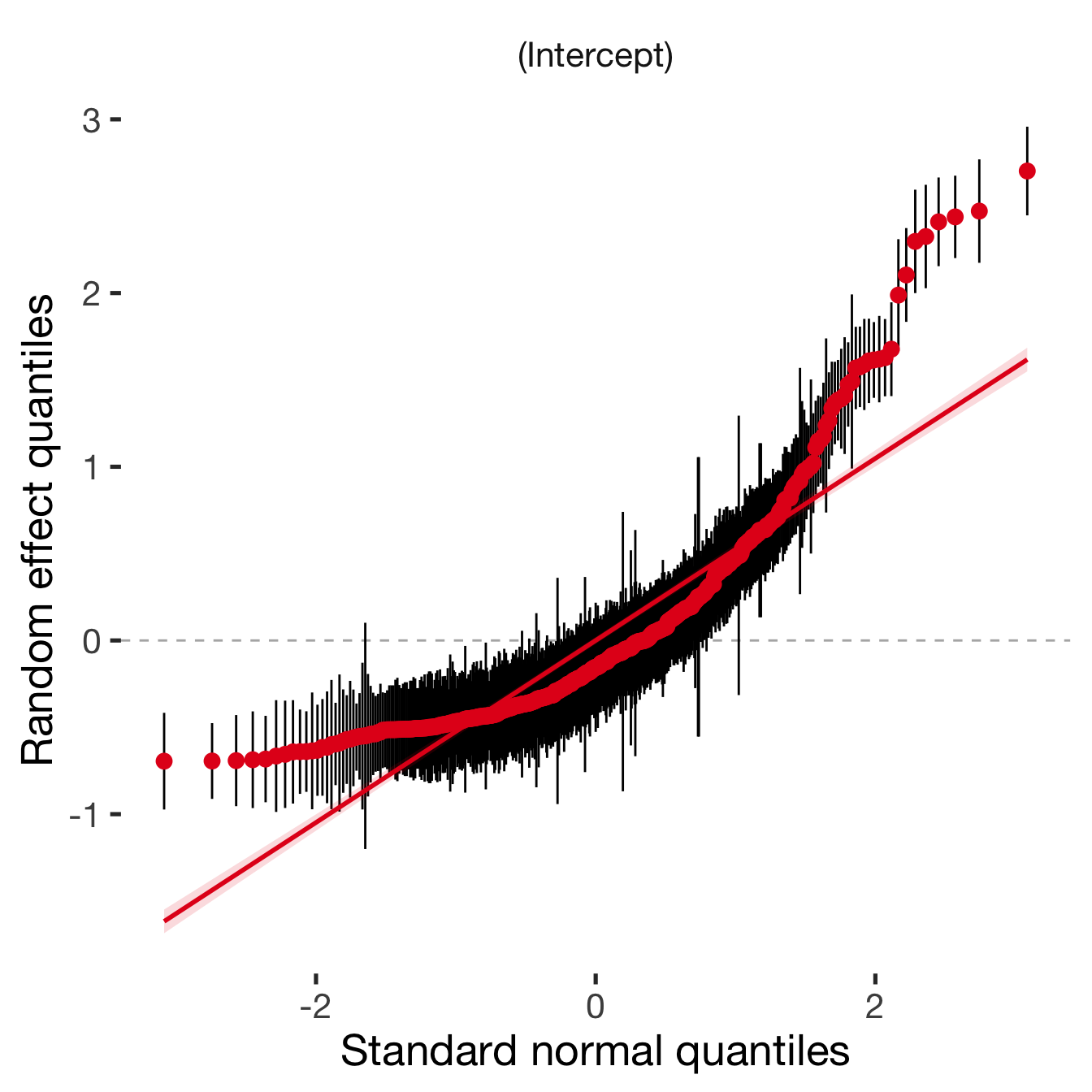
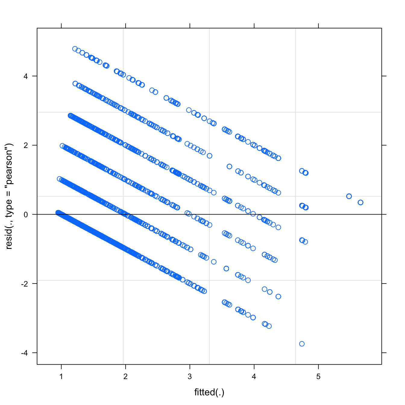
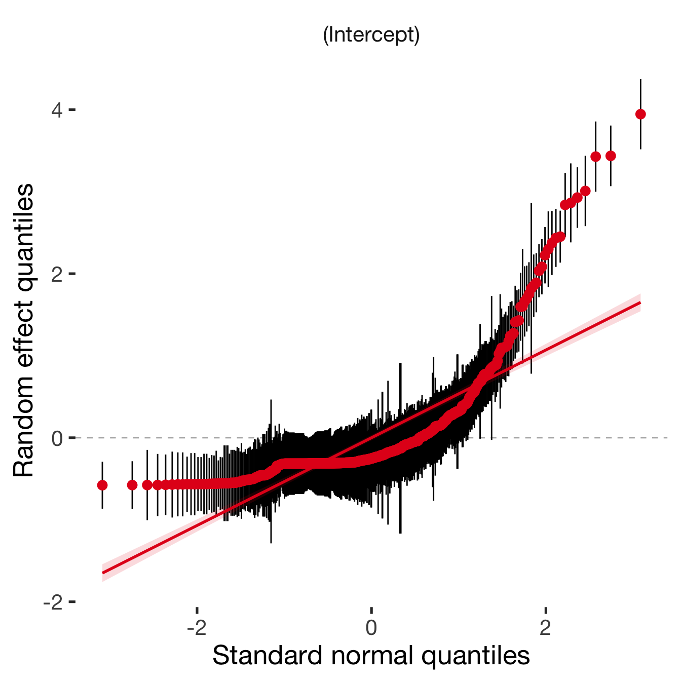
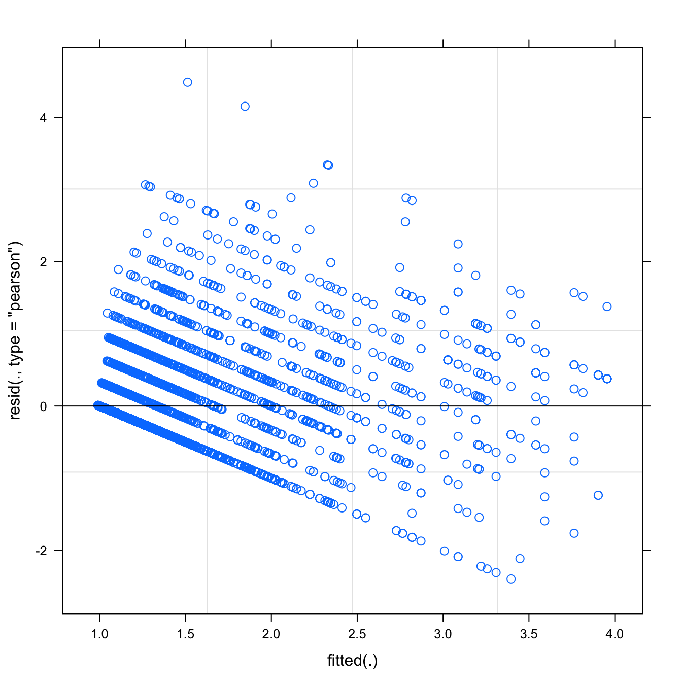
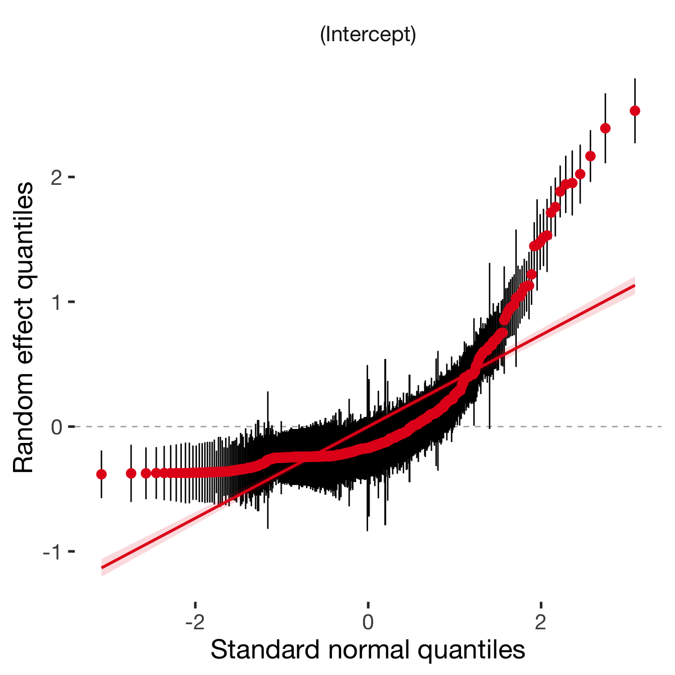
Diagnostics
model %>%
  plot_outcome(diary) %>%
  print_diagnostics()
## Error in qqnorm.default(resid(obj)): y is empty or has only NAs
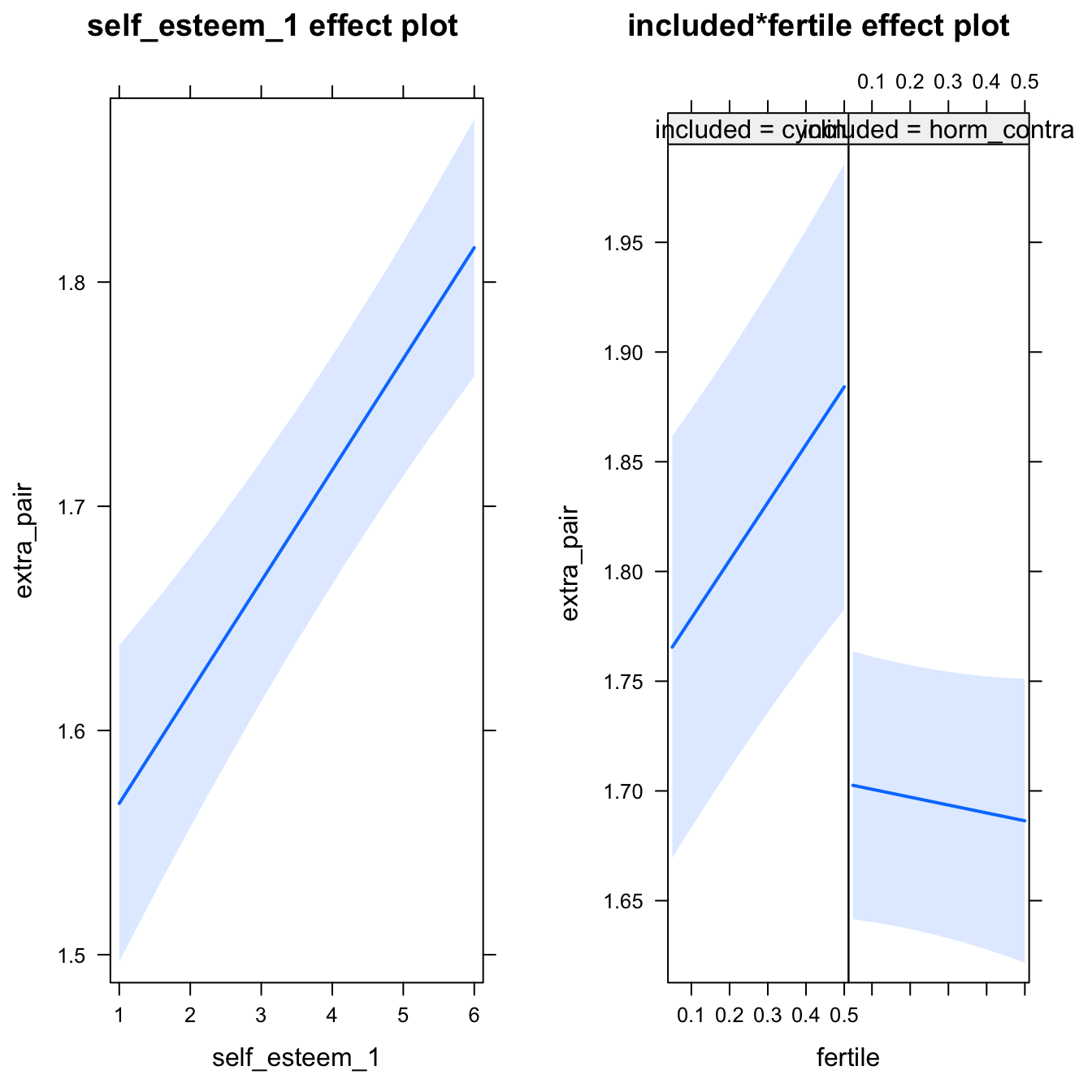
Adjusting for self esteem
model %>%
  adjust_for_self_esteem(diary)
##
##
## ```
## Linear mixed model fit by REML. t-tests use Satterthwaite's method ['lmerModLmerTest']
## Formula: form
## Data: diary
##
## REML criterion at convergence: 11307
##
## Scaled residuals:
## Min 1Q Median 3Q Max
## -4.453 -0.543 -0.142 0.412 7.517
##
## Random effects:
## Groups Name Variance Std.Dev.
## person (Intercept) 0.305 0.552
## Residual 0.280 0.529
## Number of obs: 6378, groups: person, 493
##
## Fixed effects:
## Estimate Std. Error df t value Pr(>|t|)
## (Intercept) 1.5412 0.0596 1046.1239 25.85 < 2e-16 ***
## includedhorm_contra -0.0480 0.0588 539.6460 -0.82 0.41
## fertile 0.2636 0.0592 5933.2999 4.45 0.00000875608 ***
## self_esteem_1 0.0496 0.0077 6335.3270 6.44 0.00000000013 ***
## includedhorm_contra:fertile -0.2996 0.0709 5936.7040 -4.22 0.00002449245 ***
## ---
## Signif. codes: 0 '***' 0.001 '**' 0.01 '*' 0.05 '.' 0.1 ' ' 1
##
## Correlation of Fixed Effects:
## (Intr) incld_ fertil slf__1
## inclddhrm_c -0.709
## fertile -0.185 0.190
## self_estm_1 -0.555 0.012 -0.004
## inclddhrm_: 0.159 -0.227 -0.835 -0.005
##
## ```
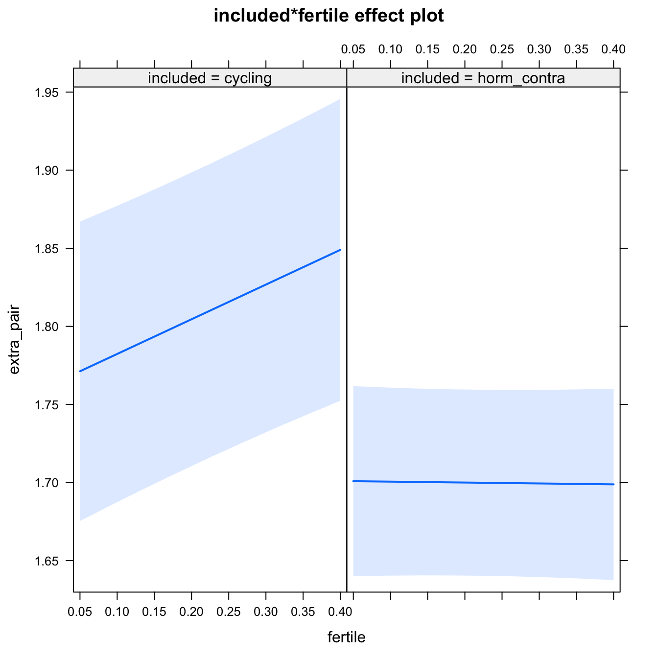
Broad window
outcome = names(model@frame)[1]
broad_models[[outcome]] <<- model %>%
  switch_window_to_broad(diary)
Linear mixed model fit by REML. t-tests use Satterthwaite's method ['lmerModLmerTest']
Formula: form
Data: diary2
REML criterion at convergence: 13739
Scaled residuals:
Min 1Q Median 3Q Max
-4.014 -0.541 -0.145 0.408 7.874
Random effects:
Groups Name Variance Std.Dev.
person (Intercept) 0.302 0.550
Residual 0.289 0.537
Number of obs: 7740, groups: person, 493
Fixed effects:
Estimate Std. Error df t value Pr(>|t|)
(Intercept) 1.7601 0.0496 555.2525 35.50 < 2e-16 ***
includedhorm_contra -0.0590 0.0587 557.9895 -1.00 0.31591
fertile 0.2221 0.0603 7311.0047 3.68 0.00023 ***
includedhorm_contra:fertile -0.2279 0.0721 7315.9296 -3.16 0.00157 **
---
Signif. codes: 0 '***' 0.001 '**' 0.01 '*' 0.05 '.' 0.1 ' ' 1
Correlation of Fixed Effects:
(Intr) incld_ fertil
inclddhrm_c -0.844
fertile -0.255 0.215
inclddhrm_: 0.213 -0.258 -0.837
Diagnostics
## Warning: 'sjp.lmer' is deprecated.
## Use 'plot_model' instead.
## See help("Deprecated")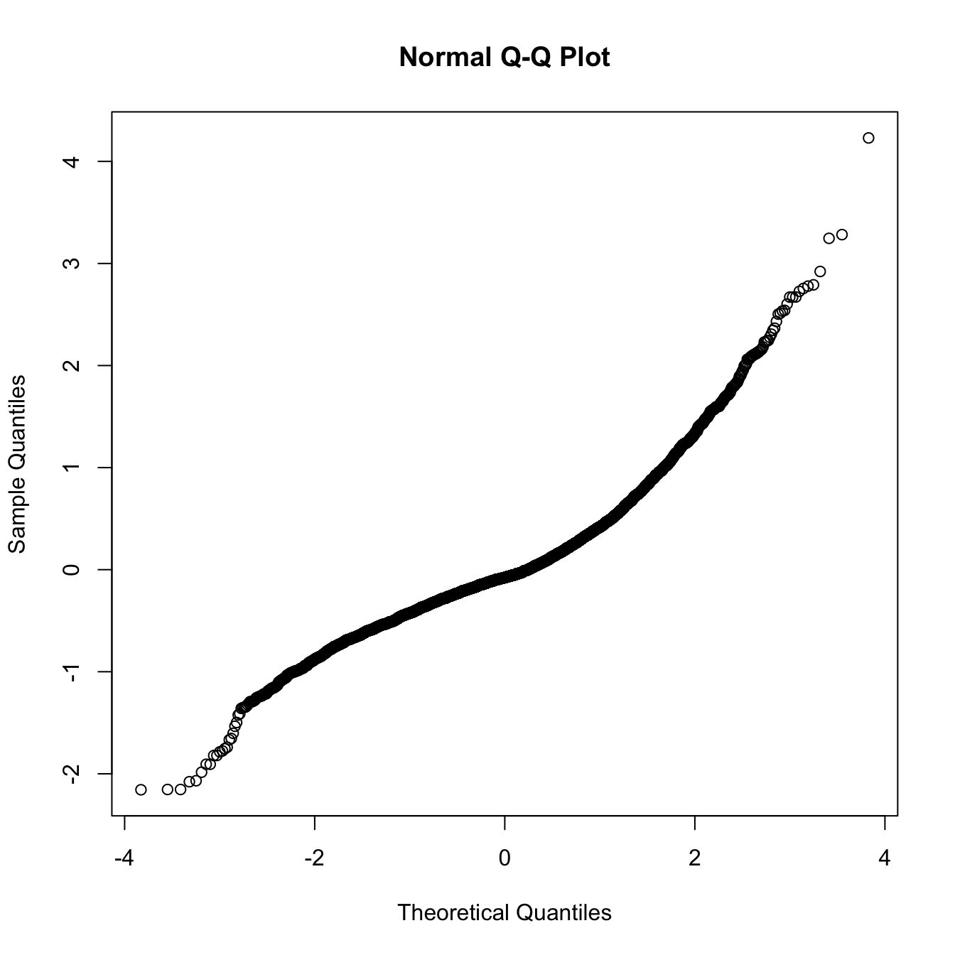
## Warning: 'sjp.lmer' is deprecated.
## Use 'plot_model' instead.
## See help("Deprecated")
Adjusting for self esteem
broad_models[[outcome]] %>%
  adjust_for_self_esteem(diary2)
##
##
## ```
## Linear mixed model fit by REML. t-tests use Satterthwaite's method ['lmerModLmerTest']
## Formula: form
## Data: diary
##
## REML criterion at convergence: 13690
##
## Scaled residuals:
## Min 1Q Median 3Q Max
## -3.916 -0.544 -0.147 0.412 7.705
##
## Random effects:
## Groups Name Variance Std.Dev.
## person (Intercept) 0.302 0.549
## Residual 0.286 0.535
## Number of obs: 7740, groups: person, 493
##
## Fixed effects:
## Estimate Std. Error df t value Pr(>|t|)
## (Intercept) 1.53263 0.05801 996.45051 26.42 < 2e-16 ***
## includedhorm_contra -0.05434 0.05867 557.82744 -0.93 0.35477
## fertile 0.21778 0.06010 7309.97189 3.62 0.00029 ***
## self_esteem_1 0.05297 0.00704 7696.26429 7.53 5.7e-14 ***
## includedhorm_contra:fertile -0.22915 0.07180 7314.72895 -3.19 0.00142 **
## ---
## Signif. codes: 0 '***' 0.001 '**' 0.01 '*' 0.05 '.' 0.1 ' ' 1
##
## Correlation of Fixed Effects:
## (Intr) incld_ fertil slf__1
## inclddhrm_c -0.726
## fertile -0.212 0.215
## self_estm_1 -0.521 0.010 -0.010
## inclddhrm_: 0.183 -0.257 -0.837 -0.002
##
## ```
bla = 2do_moderators(models$extra_pair, diary)Moderators
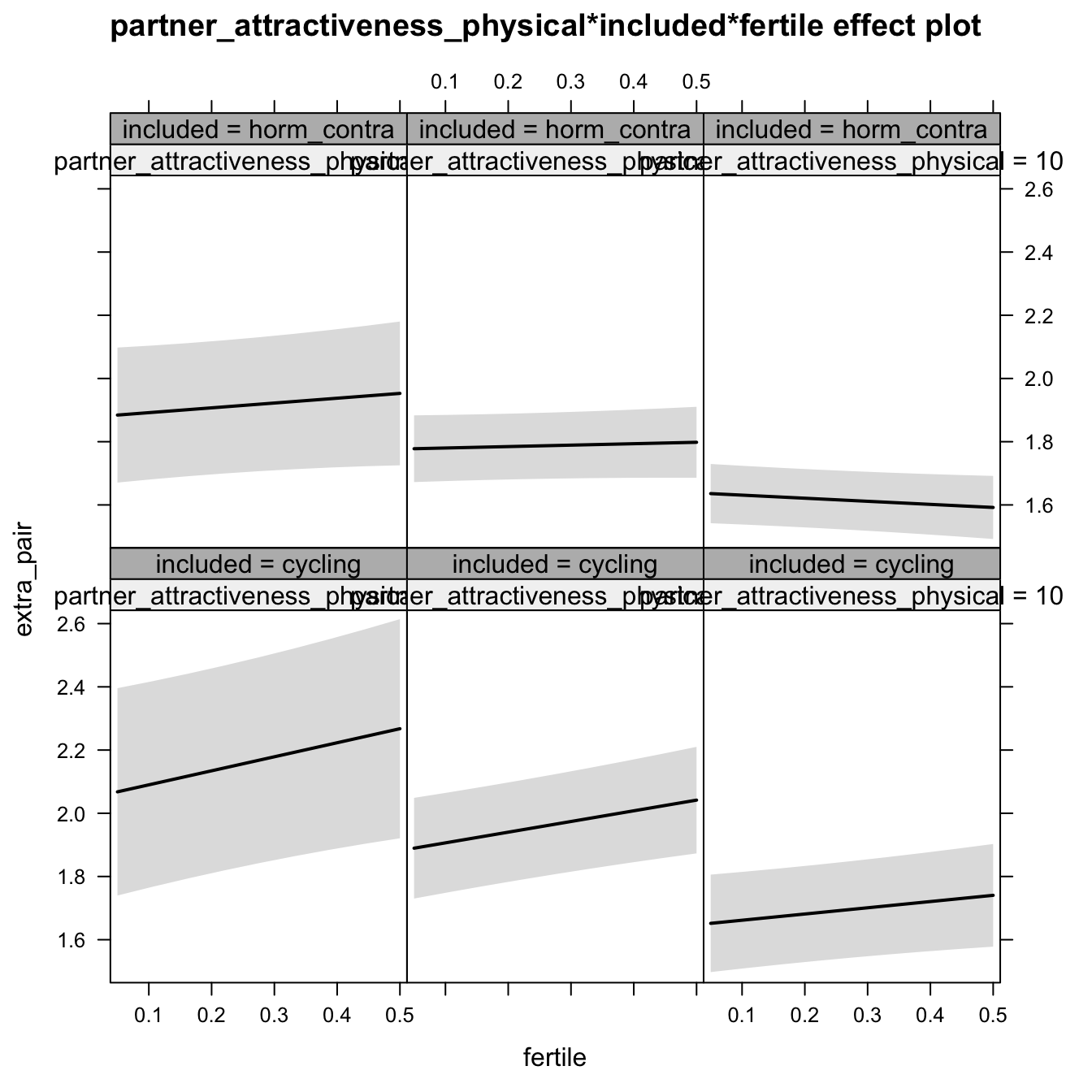
H2_1 Partner’s physical attractiveness
Predicted fertile phase effect sizes (in red): biggest (EP desire, partner mate retention)/smallest (IP desire) when partner’s physical attractiveness is low.
model %>%
test_moderator("partner_attractiveness_physical", diary)| Df | AIC | BIC | logLik | deviance | Chisq | Chi Df | Pr(>Chisq) | |
|---|---|---|---|---|---|---|---|---|
| with_main | 8 | 11330 | 11385 | -5657 | 11314 | NA | NA | NA |
| with_mod | 10 | 11332 | 11399 | -5656 | 11312 | 2.756 | 2 | 0.2521 |
Linear mixed model fit by REML. t-tests use Satterthwaite's method ['lmerModLmerTest']
Formula: extra_pair ~ (1 | person) + partner_attractiveness_physical +
    included + fertile + partner_attractiveness_physical:included +
    partner_attractiveness_physical:fertile + included:fertile +
    partner_attractiveness_physical:included:fertile
   Data: diary

REML criterion at convergence: 11351

Scaled residuals:
   Min     1Q Median     3Q    Max
-4.514 -0.543 -0.142  0.412  7.674

Random effects:
 Groups   Name        Variance Std.Dev.
 person   (Intercept) 0.301    0.549
 Residual             0.282    0.531
Number of obs: 6378, groups:  person, 493

Fixed effects:
                                                               Estimate  Std. Error          df t value
(Intercept)                                                    2.218603    0.262724  531.771799    8.44
partner_attractiveness_physical                               -0.057670    0.032051  532.726625   -1.80
includedhorm_contra                                           -0.240812    0.312893  535.501361   -0.77
fertile                                                        0.549603    0.311898 5925.089869    1.76
partner_attractiveness_physical:includedhorm_contra            0.023959    0.037989  536.608359    0.63
partner_attractiveness_physical:fertile                       -0.035256    0.038004 5928.135305   -0.93
includedhorm_contra:fertile                                   -0.290330    0.379106 5933.097116   -0.77
partner_attractiveness_physical:includedhorm_contra:fertile   -0.000411    0.046007 5935.193922   -0.01
                                                            Pr(>|t|)
(Intercept)                                                  2.9e-16 ***
partner_attractiveness_physical                                0.073 .
includedhorm_contra                                            0.442
fertile                                                        0.078 .
partner_attractiveness_physical:includedhorm_contra            0.529
partner_attractiveness_physical:fertile                        0.354
includedhorm_contra:fertile                                    0.444
partner_attractiveness_physical:includedhorm_contra:fertile    0.993
---
Signif. codes:  0 '***' 0.001 '**' 0.01 '*' 0.05 '.' 0.1 ' ' 1

Correlation of Fixed Effects:
            (Intr) prtn__ incld_ fertil pr__:_ prt__: incl_:
prtnr_ttrc_ -0.982
inclddhrm_c -0.840  0.825
fertile     -0.220  0.217  0.185
prtnr_tt_:_  0.829 -0.844 -0.982 -0.183
prtnr_ttr_:  0.217 -0.222 -0.182 -0.982  0.187
inclddhrm_:  0.181 -0.178 -0.224 -0.823  0.221  0.808
prtnr_t_:_: -0.179  0.183  0.221  0.811 -0.225 -0.826 -0.982
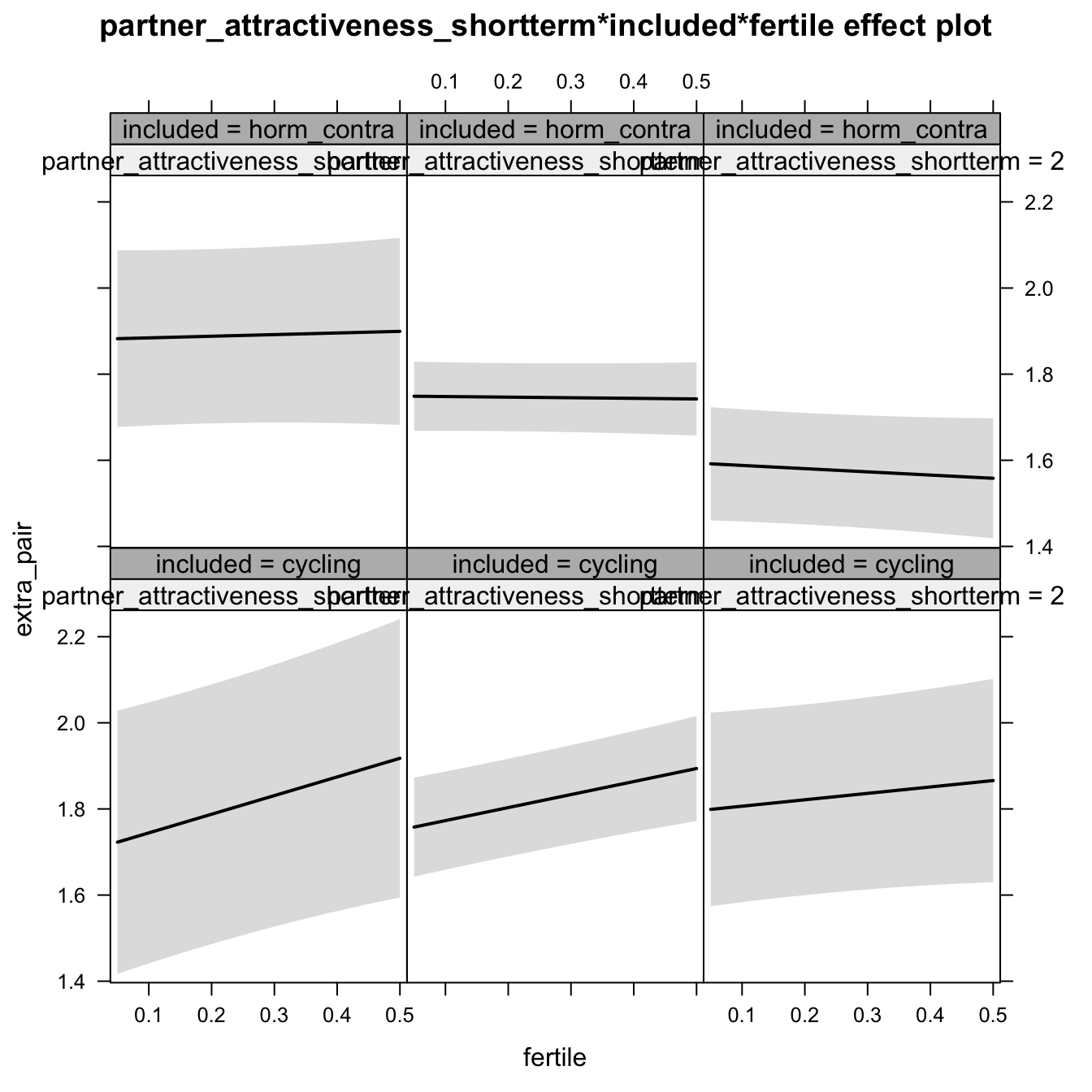
H2_1 Partner’s short-term attractiveness
Predicted fertile phase effect sizes (in red): biggest (EP desire, partner mate retention)/smallest (IP desire) when partner’s short-term attractiveness is low.
model %>%
test_moderator("partner_attractiveness_shortterm", diary)| Df | AIC | BIC | logLik | deviance | Chisq | Chi Df | Pr(>Chisq) | |
|---|---|---|---|---|---|---|---|---|
| with_main | 8 | 11335 | 11389 | -5659 | 11319 | NA | NA | NA |
| with_mod | 10 | 11338 | 11405 | -5659 | 11318 | 1.183 | 2 | 0.5536 |
Linear mixed model fit by REML. t-tests use Satterthwaite's method ['lmerModLmerTest']
Formula: extra_pair ~ (1 | person) + partner_attractiveness_shortterm +
    included + fertile + partner_attractiveness_shortterm:included +
    partner_attractiveness_shortterm:fertile + included:fertile +
    partner_attractiveness_shortterm:included:fertile
   Data: diary

REML criterion at convergence: 11353

Scaled residuals:
   Min     1Q Median     3Q    Max
-4.511 -0.545 -0.141  0.412  7.683

Random effects:
 Groups   Name        Variance Std.Dev.
 person   (Intercept) 0.304    0.551
 Residual             0.282    0.531
Number of obs: 6378, groups:  person, 493

Fixed effects:
                                                              Estimate Std. Error        df t value Pr(>|t|)
(Intercept)                                                     1.7553     0.0497  535.6669   35.35  < 2e-16
partner_attractiveness_shortterm                                0.0181     0.0509  545.1232    0.35     0.72
includedhorm_contra                                            -0.0458     0.0590  537.6109   -0.78     0.44
fertile                                                         0.2626     0.0595 5932.1602    4.41 0.000010
partner_attractiveness_shortterm:includedhorm_contra           -0.0751     0.0603  543.7968   -1.24     0.21
partner_attractiveness_shortterm:fertile                       -0.0568     0.0613 5946.8207   -0.93     0.35
includedhorm_contra:fertile                                    -0.2922     0.0714 5935.3670   -4.09 0.000043
partner_attractiveness_shortterm:includedhorm_contra:fertile    0.0343     0.0730 5944.5893    0.47     0.64

(Intercept)                                                  ***
partner_attractiveness_shortterm
includedhorm_contra
fertile                                                      ***
partner_attractiveness_shortterm:includedhorm_contra
partner_attractiveness_shortterm:fertile
includedhorm_contra:fertile                                  ***
partner_attractiveness_shortterm:includedhorm_contra:fertile
---
Signif. codes:  0 '***' 0.001 '**' 0.01 '*' 0.05 '.' 0.1 ' ' 1

Correlation of Fixed Effects:
            (Intr) prtn__ incld_ fertil pr__:_ prt__: incl_:
prtnr_ttrc_  0.062
inclddhrm_c -0.842 -0.052
fertile     -0.226 -0.018  0.191
prtnr_tt_:_ -0.052 -0.845  0.004  0.015
prtnr_ttr_: -0.018 -0.230  0.015  0.043  0.194
inclddhrm_:  0.189  0.015 -0.228 -0.834 -0.005 -0.036
prtnr_t_:_:  0.015  0.193 -0.005 -0.036 -0.231 -0.839 -0.004
H2_1 Partner’s short-term vs long-term attractiveness
Predicted fertile phase effect sizes (in red): biggest (EP desire, partner mate retention)/smallest (IP desire) top-right (high LT, low ST), then top-left (low LT, low ST), then bottom-left (low LT, high ST), then bottom-right (high LT/ST).
add_main = update.formula(formula(model), new = as.formula(paste0(". ~ . + partner_attractiveness_longterm * included + partner_attractiveness_shortterm * included + partner_attractiveness_longterm * partner_attractiveness_shortterm"))) # reorder so that the triptych looks nice
add_mod_formula = update.formula(update.formula(formula(model), new = . ~ . - included * fertile), new = as.formula(paste0(". ~ . + partner_attractiveness_longterm * fertile * partner_attractiveness_shortterm * included"))) # reorder so that the triptych looks nice

update(model, formula = add_main) -> with_main
update(model, formula = add_mod_formula) -> with_mod
if (is(with_mod, "lmerMod")) {
  with_mod <- as_lmerModLmerTest(with_mod)
}
cat(pander(anova(with_main, with_mod)))| Df | AIC | BIC | logLik | deviance | Chisq | Chi Df | Pr(>Chisq) | |
|---|---|---|---|---|---|---|---|---|
| with_main | 11 | 11315 | 11390 | -5647 | 11293 | NA | NA | NA |
| with_mod | 18 | 11325 | 11446 | -5644 | 11289 | 4.695 | 7 | 0.6972 |
effs = allEffects(with_mod)
effs = data.frame(effs$`partner_attractiveness_longterm:fertile:partner_attractiveness_shortterm:included`) %>%
  filter(round(partner_attractiveness_longterm,1) %in% c(-3,-2,0.8),round(partner_attractiveness_shortterm,1) %in% c(-2,0.5, 2))
ggplot(effs, aes(fertile, fit, ymin = lower, ymax = upper, color = included)) +
  facet_grid(partner_attractiveness_shortterm ~ partner_attractiveness_longterm) +
  geom_smooth(stat='identity') +
  scale_color_manual(values = c("cycling" = 'red', 'horm_contra' = 'black'), guide = F) +
  scale_fill_manual(values = c("cycling" = 'red', 'horm_contra' = 'black'), guide = F) +
  ggtitle("Moderation", "top-to-bottom: short-term,\nleft-to-right: long-term attractiveness of the partner")+
  ylab(names(model@frame)[1])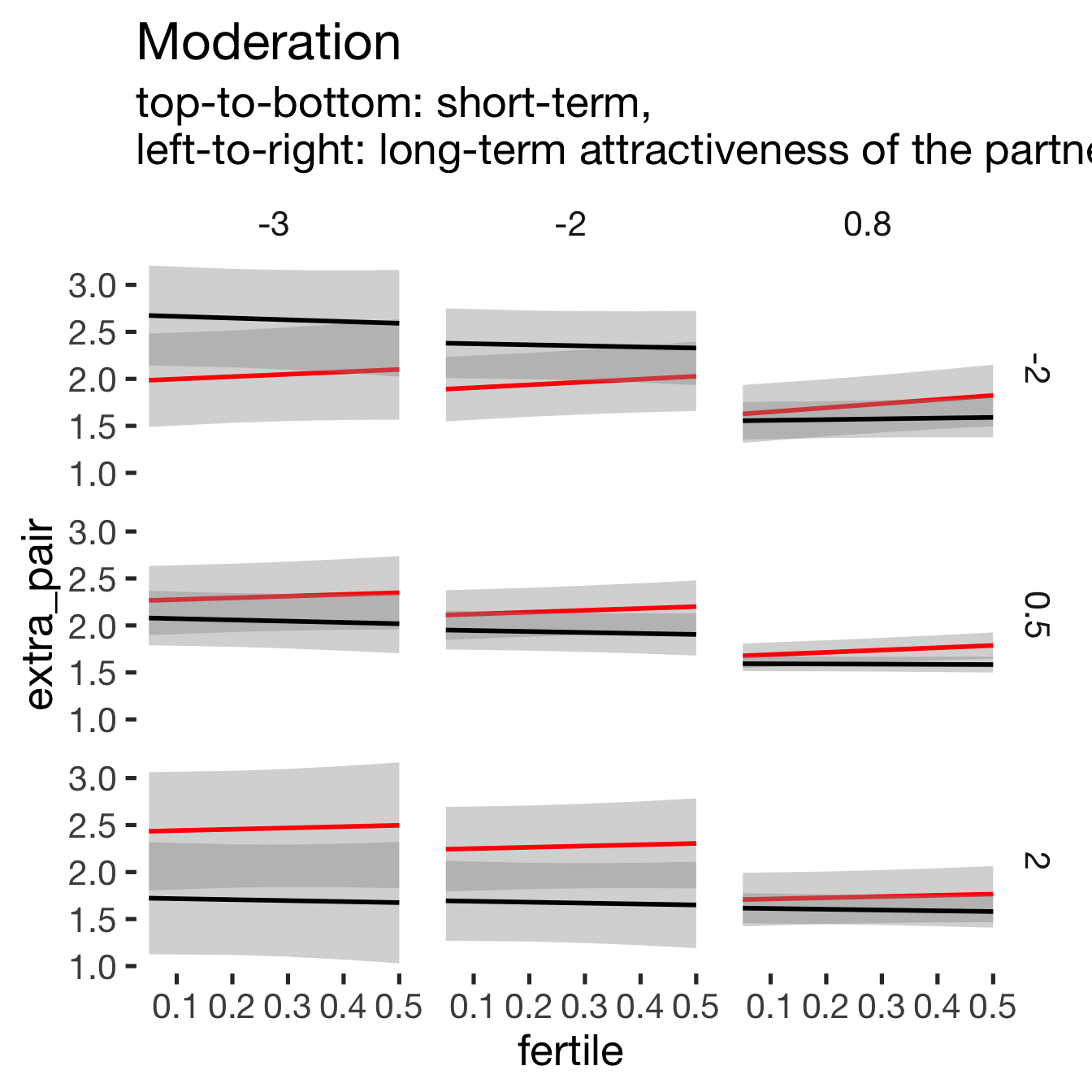
print_summary(with_mod)Linear mixed model fit by REML. t-tests use Satterthwaite's method ['lmerModLmerTest']
Formula: extra_pair ~ (1 | person) + partner_attractiveness_longterm +
fertile + partner_attractiveness_shortterm + included + partner_attractiveness_longterm:fertile +
partner_attractiveness_longterm:partner_attractiveness_shortterm +
fertile:partner_attractiveness_shortterm + partner_attractiveness_longterm:included +
fertile:included + partner_attractiveness_shortterm:included +
partner_attractiveness_longterm:fertile:partner_attractiveness_shortterm +
partner_attractiveness_longterm:fertile:included + partner_attractiveness_longterm:partner_attractiveness_shortterm:included +
fertile:partner_attractiveness_shortterm:included + partner_attractiveness_longterm:fertile:partner_attractiveness_shortterm:included
Data: diary
REML criterion at convergence: 11358
Scaled residuals:
Min 1Q Median 3Q Max
-4.523 -0.548 -0.144 0.418 7.671
Random effects:
Groups Name Variance Std.Dev.
person (Intercept) 0.288 0.537
Residual 0.282 0.531
Number of obs: 6378, groups: person, 493
Fixed effects:
Estimate
(Intercept) 1.76825
partner_attractiveness_longterm -0.14388
fertile 0.26487
partner_attractiveness_shortterm 0.04287
includedhorm_contra -0.05218
partner_attractiveness_longterm:fertile 0.02248
partner_attractiveness_longterm:partner_attractiveness_shortterm -0.02360
fertile:partner_attractiveness_shortterm -0.06686
partner_attractiveness_longterm:includedhorm_contra -0.01921
fertile:includedhorm_contra -0.29585
partner_attractiveness_shortterm:includedhorm_contra -0.07940
partner_attractiveness_longterm:fertile:partner_attractiveness_shortterm -0.01275
partner_attractiveness_longterm:fertile:includedhorm_contra 0.01523
partner_attractiveness_longterm:partner_attractiveness_shortterm:includedhorm_contra 0.09108
fertile:partner_attractiveness_shortterm:includedhorm_contra 0.03953
partner_attractiveness_longterm:fertile:partner_attractiveness_shortterm:includedhorm_contra -0.00302
Std. Error
(Intercept) 0.04933
partner_attractiveness_longterm 0.05150
fertile 0.06052
partner_attractiveness_shortterm 0.05336
includedhorm_contra 0.05891
partner_attractiveness_longterm:fertile 0.06286
partner_attractiveness_longterm:partner_attractiveness_shortterm 0.04131
fertile:partner_attractiveness_shortterm 0.06580
partner_attractiveness_longterm:includedhorm_contra 0.06446
fertile:includedhorm_contra 0.07330
partner_attractiveness_shortterm:includedhorm_contra 0.06266
partner_attractiveness_longterm:fertile:partner_attractiveness_shortterm 0.05182
partner_attractiveness_longterm:fertile:includedhorm_contra 0.08179
partner_attractiveness_longterm:partner_attractiveness_shortterm:includedhorm_contra 0.05797
fertile:partner_attractiveness_shortterm:includedhorm_contra 0.07803
partner_attractiveness_longterm:fertile:partner_attractiveness_shortterm:includedhorm_contra 0.07436
df
(Intercept) 530.92547
partner_attractiveness_longterm 521.71459
fertile 5927.20084
partner_attractiveness_shortterm 544.64550
includedhorm_contra 533.89389
partner_attractiveness_longterm:fertile 5914.86283
partner_attractiveness_longterm:partner_attractiveness_shortterm 528.98538
fertile:partner_attractiveness_shortterm 5953.85602
partner_attractiveness_longterm:includedhorm_contra 529.29006
fertile:includedhorm_contra 5935.12483
partner_attractiveness_shortterm:includedhorm_contra 543.43694
partner_attractiveness_longterm:fertile:partner_attractiveness_shortterm 5932.01295
partner_attractiveness_longterm:fertile:includedhorm_contra 5941.10648
partner_attractiveness_longterm:partner_attractiveness_shortterm:includedhorm_contra 532.93946
fertile:partner_attractiveness_shortterm:includedhorm_contra 5953.37777
partner_attractiveness_longterm:fertile:partner_attractiveness_shortterm:includedhorm_contra 5948.91692
t value Pr(>|t|)
(Intercept) 35.85 < 2e-16
partner_attractiveness_longterm -2.79 0.0054
fertile 4.38 0.000012
partner_attractiveness_shortterm 0.80 0.4221
includedhorm_contra -0.89 0.3762
partner_attractiveness_longterm:fertile 0.36 0.7207
partner_attractiveness_longterm:partner_attractiveness_shortterm -0.57 0.5681
fertile:partner_attractiveness_shortterm -1.02 0.3096
partner_attractiveness_longterm:includedhorm_contra -0.30 0.7657
fertile:includedhorm_contra -4.04 0.000055
partner_attractiveness_shortterm:includedhorm_contra -1.27 0.2057
partner_attractiveness_longterm:fertile:partner_attractiveness_shortterm -0.25 0.8057
partner_attractiveness_longterm:fertile:includedhorm_contra 0.19 0.8523
partner_attractiveness_longterm:partner_attractiveness_shortterm:includedhorm_contra 1.57 0.1167
fertile:partner_attractiveness_shortterm:includedhorm_contra 0.51 0.6125
partner_attractiveness_longterm:fertile:partner_attractiveness_shortterm:includedhorm_contra -0.04 0.9677
(Intercept) ***
partner_attractiveness_longterm **
fertile ***
partner_attractiveness_shortterm
includedhorm_contra
partner_attractiveness_longterm:fertile
partner_attractiveness_longterm:partner_attractiveness_shortterm
fertile:partner_attractiveness_shortterm
partner_attractiveness_longterm:includedhorm_contra
fertile:includedhorm_contra ***
partner_attractiveness_shortterm:includedhorm_contra
partner_attractiveness_longterm:fertile:partner_attractiveness_shortterm
partner_attractiveness_longterm:fertile:includedhorm_contra
partner_attractiveness_longterm:partner_attractiveness_shortterm:includedhorm_contra
fertile:partner_attractiveness_shortterm:includedhorm_contra
partner_attractiveness_longterm:fertile:partner_attractiveness_shortterm:includedhorm_contra
---
Signif. codes: 0 '***' 0.001 '**' 0.01 '*' 0.05 '.' 0.1 ' ' 1
H2_1b Partner’s short-term and long-term attractiveness
Edit: Alternative model specification, added after publication. Predicted fertile phase effect sizes (in red): biggest (EP desire, partner mate retention)/smallest (IP desire) top-right (high LT, low ST), then top-left (low LT, low ST), then bottom-left (low LT, high ST), then bottom-right (high LT/ST).
add_main = update.formula(formula(model), new = as.formula(paste0(". ~ . + partner_attractiveness_shortterm * included + partner_attractiveness_longterm * fertile * included"))) # reorder so that the triptych looks nice
add_mod_formula = update.formula(update.formula(formula(model), new = . ~ . - included * fertile), new = as.formula(paste0(". ~ . + (partner_attractiveness_shortterm + partner_attractiveness_longterm) * fertile * included"))) # reorder so that the triptych looks nice

update(model, formula = add_main) -> with_main
update(model, formula = add_mod_formula) -> with_mod
if (is(with_mod, "lmerMod")) {
  with_mod <- as_lmerModLmerTest(with_mod)
}
cat(pander(anova(with_main, with_mod)))| Df | AIC | BIC | logLik | deviance | Chisq | Chi Df | Pr(>Chisq) | |
|---|---|---|---|---|---|---|---|---|
| with_main | 12 | 11318 | 11399 | -5647 | 11294 | NA | NA | NA |
| with_mod | 14 | 11320 | 11415 | -5646 | 11292 | 1.541 | 2 | 0.4629 |
plot_triptych(with_mod)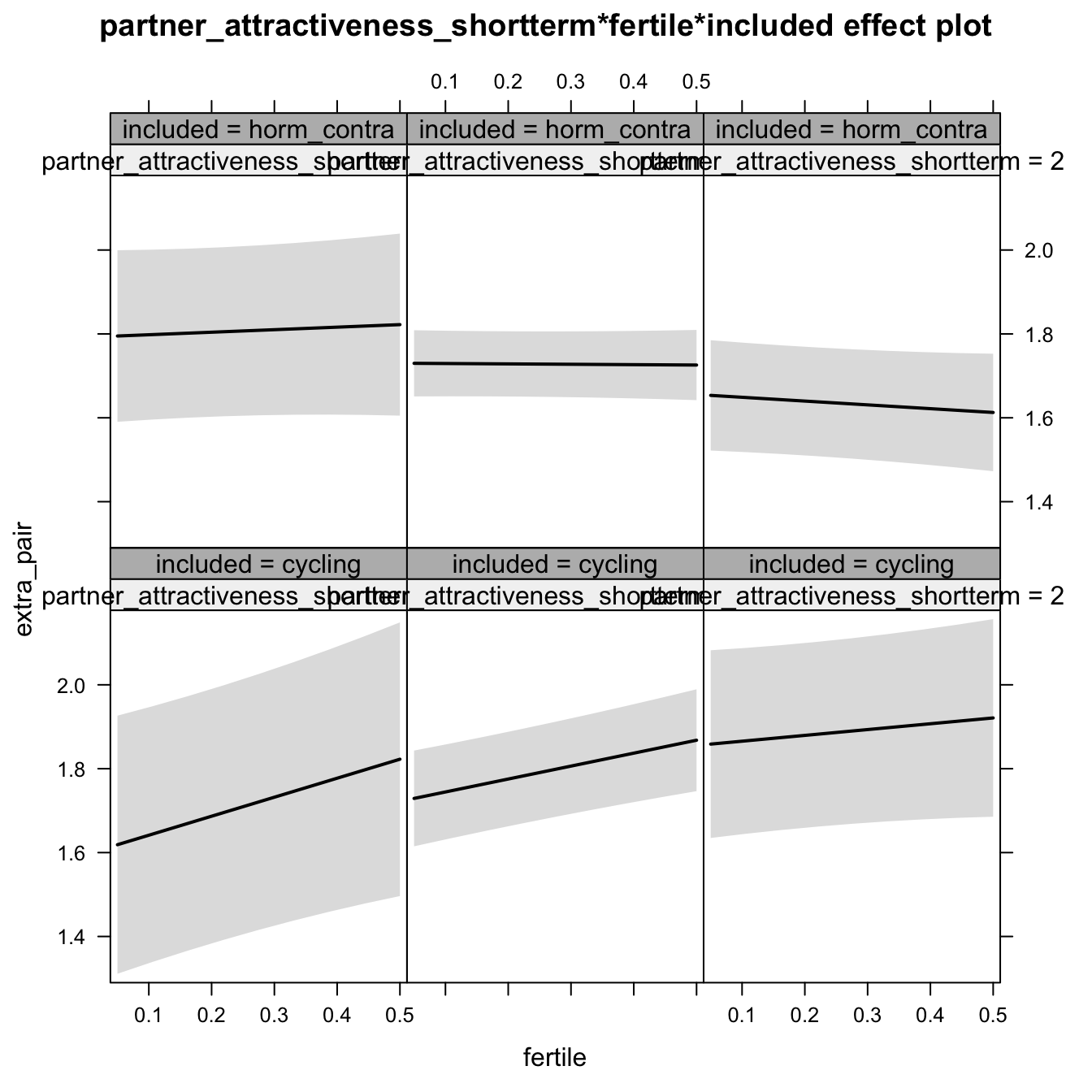
print_summary(with_mod)Linear mixed model fit by REML. t-tests use Satterthwaite's method ['lmerModLmerTest']
Formula: extra_pair ~ (1 | person) + partner_attractiveness_shortterm +
partner_attractiveness_longterm + fertile + included + partner_attractiveness_shortterm:fertile +
partner_attractiveness_longterm:fertile + partner_attractiveness_shortterm:included +
partner_attractiveness_longterm:included + fertile:included +
partner_attractiveness_shortterm:fertile:included + partner_attractiveness_longterm:fertile:included
Data: diary
REML criterion at convergence: 11344
Scaled residuals:
Min 1Q Median 3Q Max
-4.498 -0.549 -0.145 0.420 7.658
Random effects:
Groups Name Variance Std.Dev.
person (Intercept) 0.289 0.538
Residual 0.282 0.531
Number of obs: 6378, groups: person, 493
Fixed effects:
Estimate Std. Error df t value Pr(>|t|)
(Intercept) 1.7634 0.0487 534.9676 36.24 < 2e-16
partner_attractiveness_shortterm 0.0511 0.0513 543.3477 1.00 0.3192
partner_attractiveness_longterm -0.1403 0.0512 524.7949 -2.74 0.0063
fertile 0.2621 0.0595 5931.3669 4.40 0.000011
includedhorm_contra -0.0353 0.0579 537.0129 -0.61 0.5429
partner_attractiveness_shortterm:fertile -0.0629 0.0631 5944.6343 -1.00 0.3188
partner_attractiveness_longterm:fertile 0.0235 0.0626 5917.2215 0.38 0.7075
partner_attractiveness_shortterm:includedhorm_contra -0.0779 0.0606 542.7737 -1.29 0.1992
partner_attractiveness_longterm:includedhorm_contra -0.0264 0.0642 531.7236 -0.41 0.6811
fertile:includedhorm_contra -0.2962 0.0717 5936.2035 -4.13 0.000037
partner_attractiveness_shortterm:fertile:includedhorm_contra 0.0327 0.0752 5944.4730 0.44 0.6636
partner_attractiveness_longterm:fertile:includedhorm_contra 0.0158 0.0813 5940.3744 0.19 0.8460
(Intercept) ***
partner_attractiveness_shortterm
partner_attractiveness_longterm **
fertile ***
includedhorm_contra
partner_attractiveness_shortterm:fertile
partner_attractiveness_longterm:fertile
partner_attractiveness_shortterm:includedhorm_contra
partner_attractiveness_longterm:includedhorm_contra
fertile:includedhorm_contra ***
partner_attractiveness_shortterm:fertile:includedhorm_contra
partner_attractiveness_longterm:fertile:includedhorm_contra
---
Signif. codes: 0 '***' 0.001 '**' 0.01 '*' 0.05 '.' 0.1 ' ' 1
Correlation of Fixed Effects:
(Intr) prtnr_ttrctvnss_s prtnr_ttrctvnss_l fertil incld_ prtnr_ttrctvnss_s:
prtnr_ttrctvnss_s 0.074
prtnr_ttrctvnss_l -0.060 -0.234
fertile -0.231 -0.019 0.003
inclddhrm_c -0.840 -0.062 0.050 0.194
prtnr_ttrctvnss_s: -0.019 -0.235 0.054 0.046 0.016
prtnr_ttrctvnss_l: 0.003 0.054 -0.222 -0.018 -0.003 -0.237
prtnr_ttrctvnss_s:_ -0.063 -0.846 0.198 0.016 0.023 0.199
prtnr_ttrctvnss_l:_ 0.048 0.187 -0.797 -0.003 -0.086 -0.043
frtl:ncldd_ 0.192 0.016 -0.003 -0.830 -0.233 -0.039
prtnr_ttrctvnss_s::_ 0.016 0.198 -0.046 -0.039 -0.008 -0.839
prtnr_ttrctvnss_l::_ -0.002 -0.042 0.171 0.014 0.014 0.183
prtnr_ttrctvnss_l: prtnr_ttrctvnss_s:_ prtnr_ttrctvnss_l:_ frtl:_ prtnr_ttrctvnss_s::_
prtnr_ttrctvnss_s
prtnr_ttrctvnss_l
fertile
inclddhrm_c
prtnr_ttrctvnss_s:
prtnr_ttrctvnss_l:
prtnr_ttrctvnss_s:_ -0.046
prtnr_ttrctvnss_l:_ 0.177 -0.228
frtl:ncldd_ 0.015 -0.008 0.014
prtnr_ttrctvnss_s::_ 0.199 -0.236 0.055 0.011
prtnr_ttrctvnss_l::_ -0.770 0.054 -0.227 -0.070 -0.236
H2_1c Partner’s short-term minus long-term attractiveness
Edit: Alternative model specification, added after publication. Predicted fertile phase effect sizes (in red): biggest (EP desire, partner mate retention)/smallest (IP desire) top-right (high LT, low ST), then top-left (low LT, low ST), then bottom-left (low LT, high ST), then bottom-right (high LT/ST).
add_main = update.formula(formula(model), new = as.formula(paste0(". ~ . + partner_st_vs_lt * included"))) # reorder so that the triptych looks nice
add_mod_formula = update.formula(update.formula(formula(model), new = . ~ . - included * fertile), new = as.formula(paste0(". ~ . + partner_st_vs_lt * fertile * included"))) # reorder so that the triptych looks nice

update(model, formula = add_main) -> with_main
update(model, formula = add_mod_formula) -> with_mod
if (is(with_mod, "lmerMod")) {
  with_mod <- as_lmerModLmerTest(with_mod)
}
cat(pander(anova(with_main, with_mod)))| Df | AIC | BIC | logLik | deviance | Chisq | Chi Df | Pr(>Chisq) | |
|---|---|---|---|---|---|---|---|---|
| with_main | 8 | 11332 | 11386 | -5658 | 11316 | NA | NA | NA |
| with_mod | 10 | 11334 | 11402 | -5657 | 11314 | 1.726 | 2 | 0.422 |
plot_triptych(with_mod)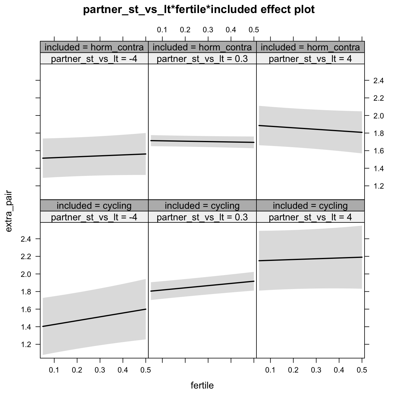
print_summary(with_mod)Linear mixed model fit by REML. t-tests use Satterthwaite's method ['lmerModLmerTest']
Formula: extra_pair ~ (1 | person) + partner_st_vs_lt + fertile + included +
partner_st_vs_lt:fertile + partner_st_vs_lt:included + fertile:included +
partner_st_vs_lt:fertile:included
Data: diary
REML criterion at convergence: 11351
Scaled residuals:
Min 1Q Median 3Q Max
-4.504 -0.548 -0.141 0.416 7.650
Random effects:
Groups Name Variance Std.Dev.
person (Intercept) 0.302 0.549
Residual 0.282 0.531
Number of obs: 6378, groups: person, 493
Fixed effects:
Estimate Std. Error df t value Pr(>|t|)
(Intercept) 1.76380 0.04959 535.56117 35.56 < 2e-16 ***
partner_st_vs_lt 0.09554 0.04102 532.12262 2.33 0.02 *
fertile 0.26227 0.05950 5931.69797 4.41 0.000011 ***
includedhorm_contra -0.06201 0.05870 538.07989 -1.06 0.29
partner_st_vs_lt:fertile -0.04327 0.04943 5928.19546 -0.88 0.38
partner_st_vs_lt:includedhorm_contra -0.04738 0.04959 535.88488 -0.96 0.34
fertile:includedhorm_contra -0.29554 0.07123 5935.72930 -4.15 0.000034 ***
partner_st_vs_lt:fertile:includedhorm_contra 0.00845 0.06091 5939.56660 0.14 0.89
---
Signif. codes: 0 '***' 0.001 '**' 0.01 '*' 0.05 '.' 0.1 ' ' 1
Correlation of Fixed Effects:
(Intr) prt___ fertil incld_ pr___: p___:_ frtl:_
prtnr_st_v_ 0.085
fertile -0.226 -0.014
inclddhrm_c -0.845 -0.072 0.191
prtnr_st__: -0.014 -0.225 0.041 0.011
prtnr_s__:_ -0.071 -0.827 0.011 0.060 0.186
frtl:ncldd_ 0.189 0.011 -0.835 -0.229 -0.034 -0.011
prtnr___::_ 0.011 0.182 -0.033 -0.011 -0.812 -0.228 0.038
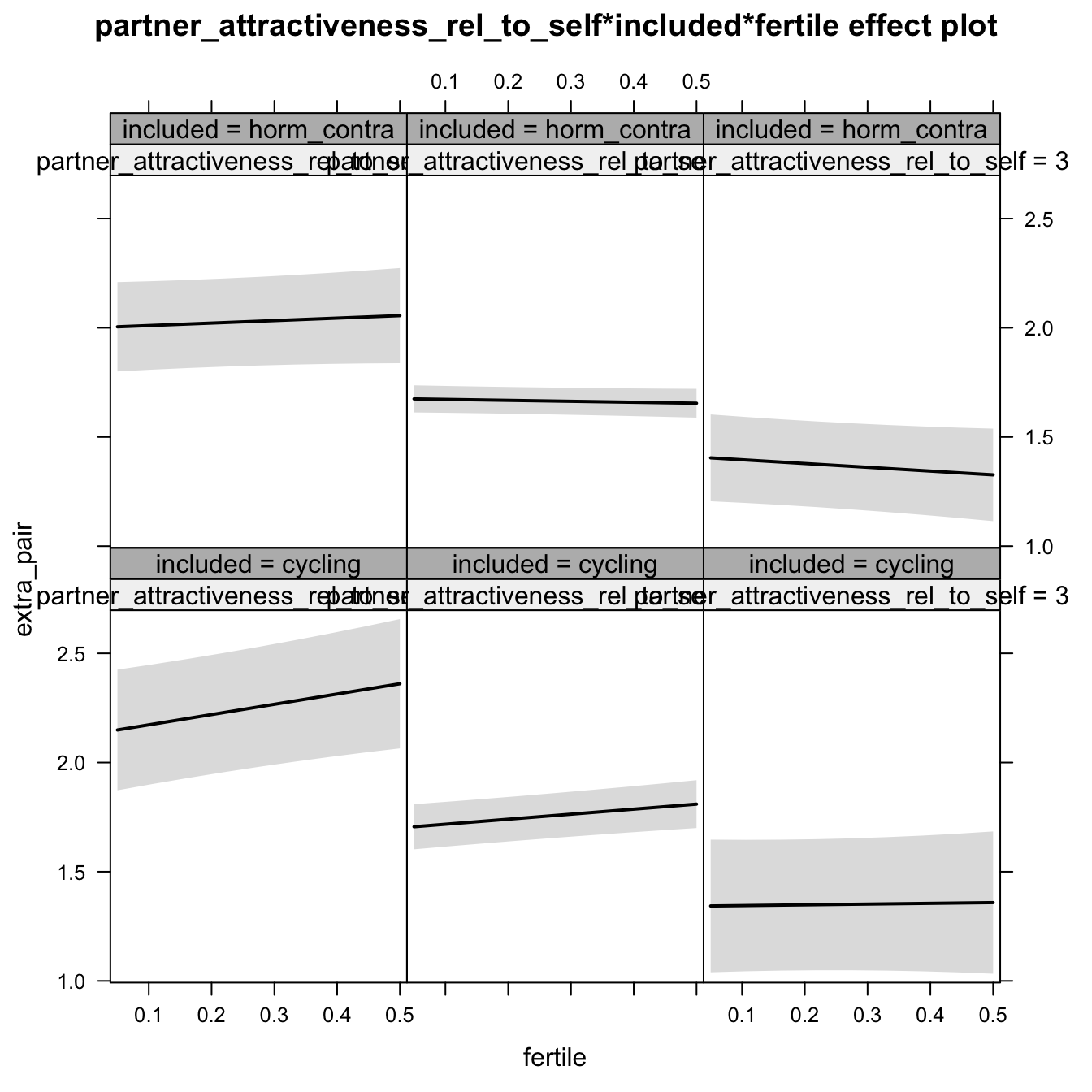
H2_3 Relative attractiveness to self
Predicted fertile phase effect sizes (in red): biggest (EP desire, partner mate retention)/smallest (IP desire) when partner’s relative attractiveness is low.
model %>%
test_moderator("partner_attractiveness_rel_to_self", diary)| Df | AIC | BIC | logLik | deviance | Chisq | Chi Df | Pr(>Chisq) | |
|---|---|---|---|---|---|---|---|---|
| with_main | 8 | 11318 | 11373 | -5651 | 11302 | NA | NA | NA |
| with_mod | 10 | 11320 | 11387 | -5650 | 11300 | 2.716 | 2 | 0.2571 |
Linear mixed model fit by REML. t-tests use Satterthwaite's method ['lmerModLmerTest']
Formula: extra_pair ~ (1 | person) + partner_attractiveness_rel_to_self +
    included + fertile + partner_attractiveness_rel_to_self:included +
    partner_attractiveness_rel_to_self:fertile + included:fertile +
    partner_attractiveness_rel_to_self:included:fertile
   Data: diary

REML criterion at convergence: 11335

Scaled residuals:
   Min     1Q Median     3Q    Max
-4.487 -0.544 -0.142  0.408  7.676

Random effects:
 Groups   Name        Variance Std.Dev.
 person   (Intercept) 0.293    0.541
 Residual             0.282    0.531
Number of obs: 6378, groups:  person, 493

Fixed effects:
                                                                Estimate Std. Error        df t value
(Intercept)                                                       1.7335     0.0493  537.1849   35.13
partner_attractiveness_rel_to_self                               -0.1307     0.0472  535.0787   -2.77
includedhorm_contra                                              -0.0276     0.0583  539.4928   -0.47
fertile                                                           0.2524     0.0604 5935.1935    4.18
partner_attractiveness_rel_to_self:includedhorm_contra            0.0330     0.0577  538.7554    0.57
partner_attractiveness_rel_to_self:fertile                       -0.0727     0.0610 5952.1461   -1.19
includedhorm_contra:fertile                                      -0.2822     0.0720 5938.3123   -3.92
partner_attractiveness_rel_to_self:includedhorm_contra:fertile    0.0248     0.0741 5950.6650    0.33
                                                               Pr(>|t|)
(Intercept)                                                     < 2e-16 ***
partner_attractiveness_rel_to_self                               0.0058 **
includedhorm_contra                                              0.6361
fertile                                                        0.000029 ***
partner_attractiveness_rel_to_self:includedhorm_contra           0.5672
partner_attractiveness_rel_to_self:fertile                       0.2337
includedhorm_contra:fertile                                    0.000090 ***
partner_attractiveness_rel_to_self:includedhorm_contra:fertile   0.7379
---
Signif. codes:  0 '***' 0.001 '**' 0.01 '*' 0.05 '.' 0.1 ' ' 1

Correlation of Fixed Effects:
            (Intr) pr____ incld_ fertil pr____:_ pr____: incl_:
prtnr_tt___  0.152
inclddhrm_c -0.847 -0.129
fertile     -0.230 -0.040  0.195
prtnr____:_ -0.125 -0.818  0.091  0.033
prtnr_t___: -0.038 -0.227  0.032  0.175  0.186
inclddhrm_:  0.193  0.034 -0.232 -0.839 -0.023   -0.147
prtn____:_:  0.031  0.187 -0.023 -0.144 -0.229   -0.823   0.104
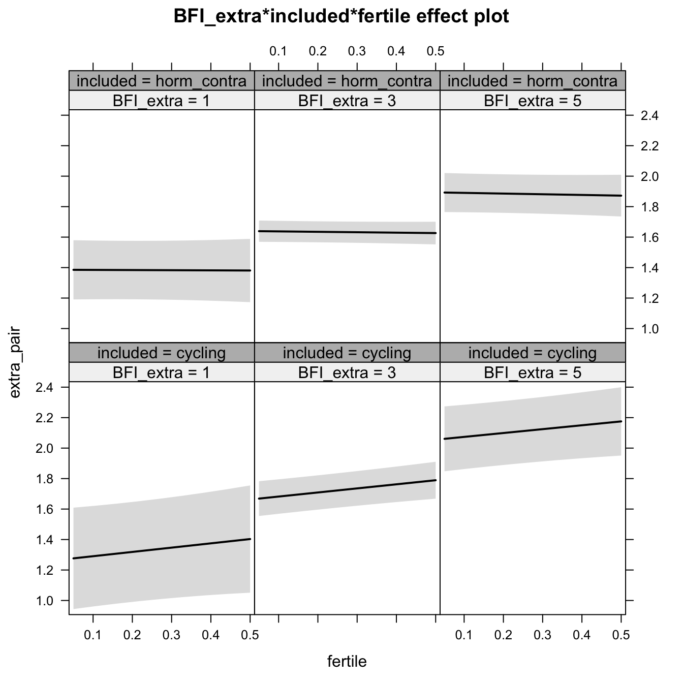
H4.1. Extraversion
models$extra_pair %>%
test_moderator("BFI_extra", diary)| Df | AIC | BIC | logLik | deviance | Chisq | Chi Df | Pr(>Chisq) | |
|---|---|---|---|---|---|---|---|---|
| with_main | 8 | 11319 | 11373 | -5651 | 11303 | NA | NA | NA |
| with_mod | 10 | 11322 | 11390 | -5651 | 11302 | 0.03857 | 2 | 0.9809 |
Linear mixed model fit by REML. t-tests use Satterthwaite's method ['lmerModLmerTest']
Formula: extra_pair ~ (1 | person) + BFI_extra + included + fertile +
    BFI_extra:included + BFI_extra:fertile + included:fertile +      BFI_extra:included:fertile
   Data: diary

REML criterion at convergence: 11336

Scaled residuals:
   Min     1Q Median     3Q    Max
-4.570 -0.546 -0.148  0.412  7.654

Random effects:
 Groups   Name        Variance Std.Dev.
 person   (Intercept) 0.293    0.542
 Residual             0.282    0.531
Number of obs: 6378, groups:  person, 493

Fixed effects:
                                        Estimate Std. Error         df t value  Pr(>|t|)
(Intercept)                              1.06591    0.23572  536.75235    4.52 0.0000075 ***
BFI_extra                                0.19645    0.06582  536.93914    2.98     0.003 **
includedhorm_contra                      0.19273    0.27297  538.81051    0.71     0.480
fertile                                  0.28834    0.28834 5916.99115    1.00     0.317
BFI_extra:includedhorm_contra           -0.06921    0.07627  539.06785   -0.91     0.365
BFI_extra:fertile                       -0.00682    0.07993 5914.81120   -0.09     0.932
includedhorm_contra:fertile             -0.28964    0.33825 5924.11336   -0.86     0.392
BFI_extra:includedhorm_contra:fertile   -0.00196    0.09405 5922.93569   -0.02     0.983
---
Signif. codes:  0 '***' 0.001 '**' 0.01 '*' 0.05 '.' 0.1 ' ' 1

Correlation of Fixed Effects:
            (Intr) BFI_xt incld_ fertil BFI_x:_ BFI_x: incl_:
BFI_extra   -0.978
inclddhrm_c -0.864  0.845
fertile     -0.232  0.226  0.200
BFI_xtr:nc_  0.844 -0.863 -0.977 -0.195
BFI_xtr:frt  0.228 -0.232 -0.197 -0.979  0.200
inclddhrm_:  0.198 -0.193 -0.232 -0.852  0.226   0.834
BFI_xtr:n_: -0.193  0.197  0.227  0.832 -0.232  -0.850 -0.978
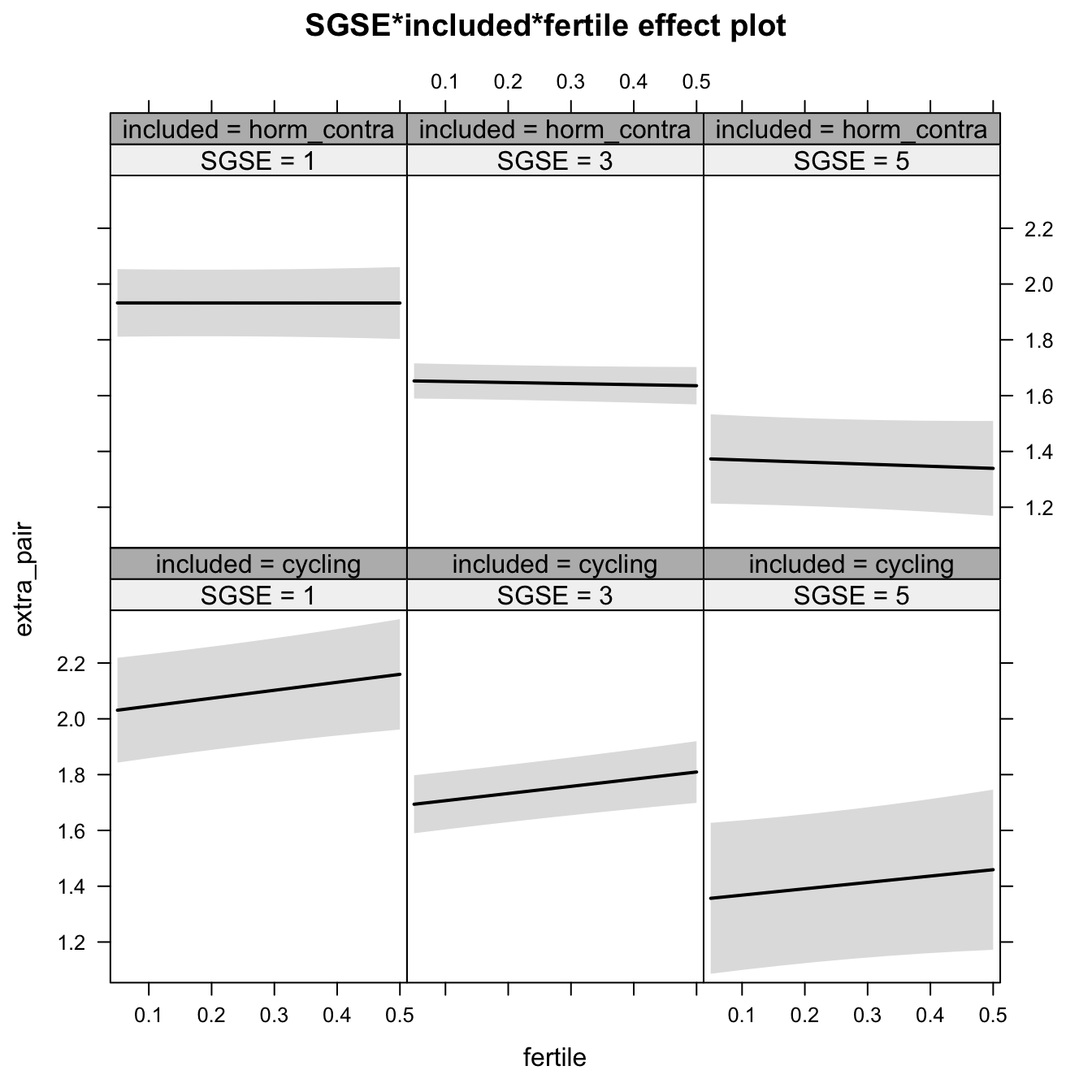
H4.2. Shyness
models$extra_pair %>%
test_moderator("SGSE", diary)| Df | AIC | BIC | logLik | deviance | Chisq | Chi Df | Pr(>Chisq) | |
|---|---|---|---|---|---|---|---|---|
| with_main | 8 | 11309 | 11363 | -5646 | 11293 | NA | NA | NA |
| with_mod | 10 | 11313 | 11380 | -5646 | 11293 | 0.2445 | 2 | 0.8849 |
Linear mixed model fit by REML. t-tests use Satterthwaite's method ['lmerModLmerTest']
Formula: extra_pair ~ (1 | person) + SGSE + included + fertile + SGSE:included +
    SGSE:fertile + included:fertile + SGSE:included:fertile
   Data: diary

REML criterion at convergence: 11328

Scaled residuals:
   Min     1Q Median     3Q    Max
-4.566 -0.542 -0.143  0.412  7.657

Random effects:
 Groups   Name        Variance Std.Dev.
 person   (Intercept) 0.287    0.536
 Residual             0.282    0.531
Number of obs: 6378, groups:  person, 493

Fixed effects:
                                   Estimate Std. Error         df t value Pr(>|t|)
(Intercept)                         2.18448    0.14623  534.71858   14.94   <2e-16 ***
SGSE                               -0.16784    0.05384  536.69677   -3.12   0.0019 **
includedhorm_contra                -0.11326    0.17314  538.92588   -0.65   0.5133
fertile                             0.30012    0.17772 5918.42545    1.69   0.0913 .
SGSE:includedhorm_contra            0.02897    0.06307  539.83464    0.46   0.6462
SGSE:fertile                       -0.01445    0.06631 5922.34831   -0.22   0.8275
includedhorm_contra:fertile        -0.28235    0.21366 5925.55710   -1.32   0.1864
SGSE:includedhorm_contra:fertile   -0.00415    0.07848 5926.91492   -0.05   0.9578
---
Signif. codes:  0 '***' 0.001 '**' 0.01 '*' 0.05 '.' 0.1 ' ' 1

Correlation of Fixed Effects:
            (Intr) SGSE   incld_ fertil SGSE:n_ SGSE:f incl_:
SGSE        -0.944
inclddhrm_c -0.845  0.797
fertile     -0.235  0.223  0.199
SGSE:ncldd_  0.806 -0.854 -0.944 -0.191
SGSE:fertil  0.221 -0.235 -0.186 -0.942  0.201
inclddhrm_:  0.196 -0.186 -0.237 -0.832  0.224   0.784
SGSE:ncld_: -0.186  0.199  0.222  0.796 -0.236  -0.845 -0.943
H4.3. Neuroticism
models$extra_pair %>%
test_moderator("BFI_neuro", diary)| Df | AIC | BIC | logLik | deviance | Chisq | Chi Df | Pr(>Chisq) | |
|---|---|---|---|---|---|---|---|---|
| with_main | 8 | 11338 | 11392 | -5661 | 11322 | NA | NA | NA |
| with_mod | 10 | 11340 | 11407 | -5660 | 11320 | 2.148 | 2 | 0.3416 |
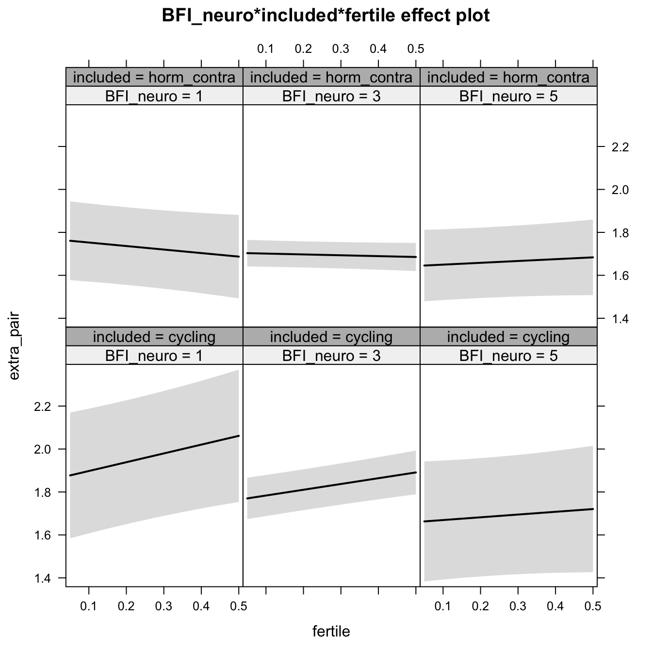
Linear mixed model fit by REML. t-tests use Satterthwaite's method ['lmerModLmerTest']
Formula: extra_pair ~ (1 | person) + BFI_neuro + included + fertile +
    BFI_neuro:included + BFI_neuro:fertile + included:fertile +      BFI_neuro:included:fertile
   Data: diary

REML criterion at convergence: 11353

Scaled residuals:
   Min     1Q Median     3Q    Max
-4.582 -0.547 -0.142  0.408  7.665

Random effects:
 Groups   Name        Variance Std.Dev.
 person   (Intercept) 0.306    0.553
 Residual             0.282    0.531
Number of obs: 6378, groups:  person, 493

Fixed effects:
                                       Estimate Std. Error        df t value Pr(>|t|)
(Intercept)                              1.9068     0.2180  541.4673    8.75   <2e-16 ***
BFI_neuro                               -0.0501     0.0695  542.1909   -0.72    0.472
includedhorm_contra                     -0.1057     0.2566  542.8916   -0.41    0.681
fertile                                  0.4797     0.2599 5938.4774    1.85    0.065 .
BFI_neuro:includedhorm_contra            0.0181     0.0814  543.6244    0.22    0.824
BFI_neuro:fertile                       -0.0703     0.0828 5928.9253   -0.85    0.396
includedhorm_contra:fertile             -0.7057     0.3089 5938.0532   -2.28    0.022 *
BFI_neuro:includedhorm_contra:fertile    0.1325     0.0978 5930.4477    1.35    0.176
---
Signif. codes:  0 '***' 0.001 '**' 0.01 '*' 0.05 '.' 0.1 ' ' 1

Correlation of Fixed Effects:
            (Intr) BFI_nr incld_ fertil BFI_n:_ BFI_n: incl_:
BFI_neuro   -0.974
inclddhrm_c -0.849  0.827
fertile     -0.229  0.223  0.195
BFI_nr:ncl_  0.832 -0.854 -0.973 -0.191
BFI_nr:frtl  0.223 -0.229 -0.190 -0.973  0.195
inclddhrm_:  0.193 -0.188 -0.230 -0.841  0.224   0.819
BFI_nr:nc_: -0.189  0.194  0.224  0.824 -0.230  -0.847 -0.973
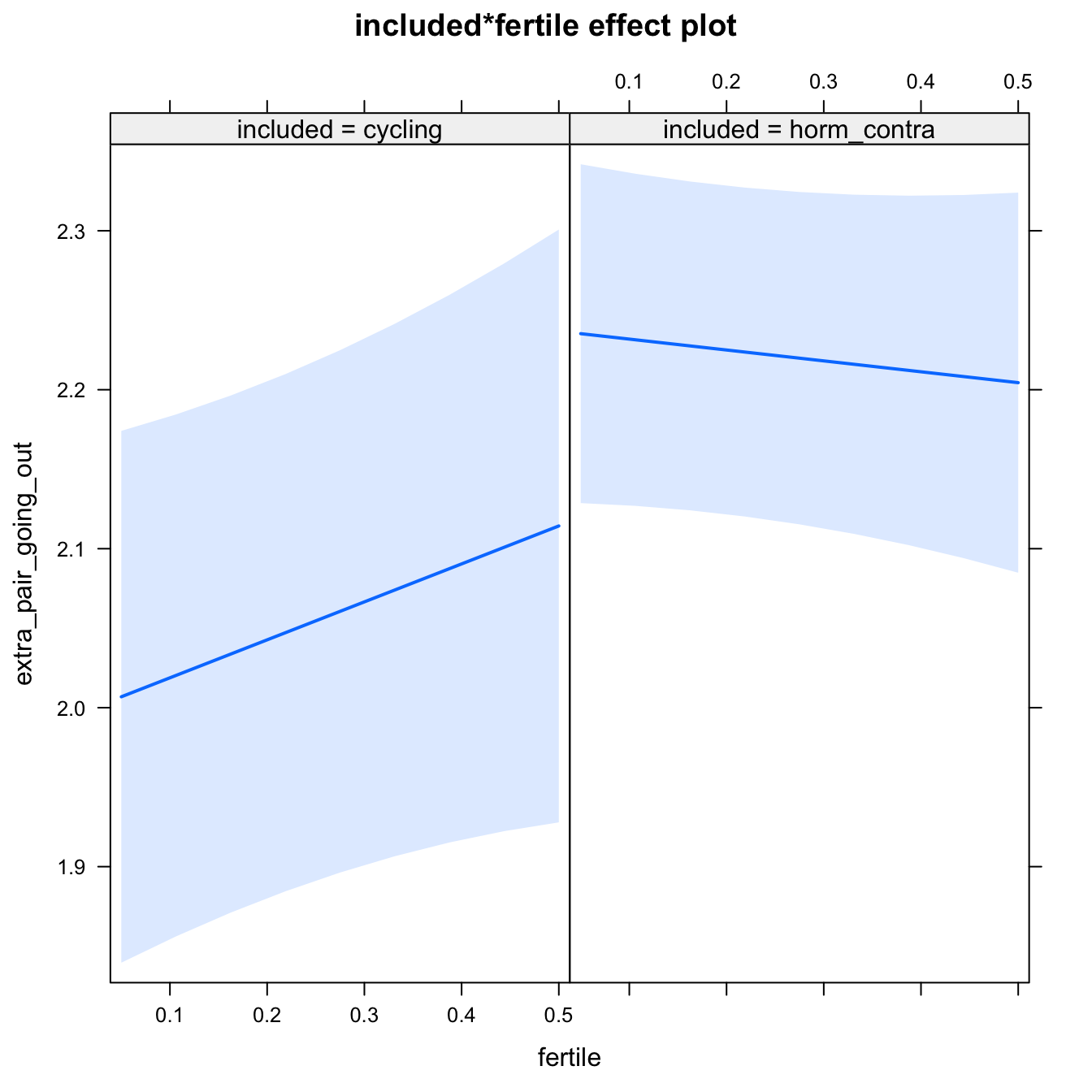
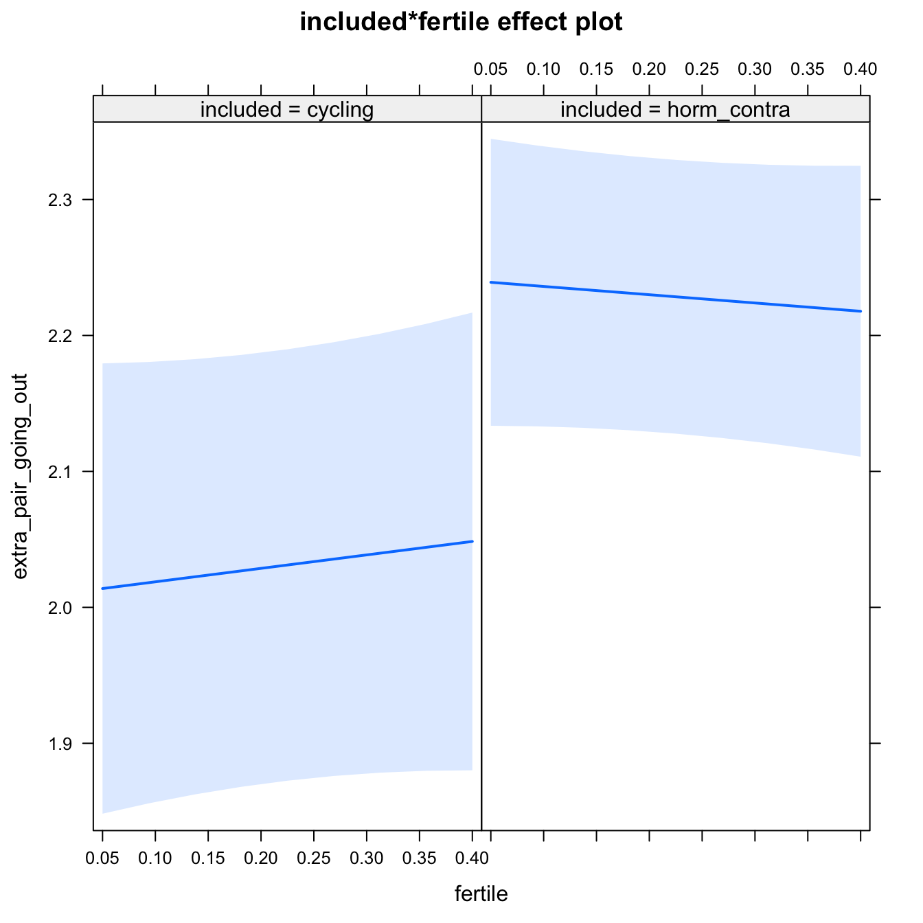
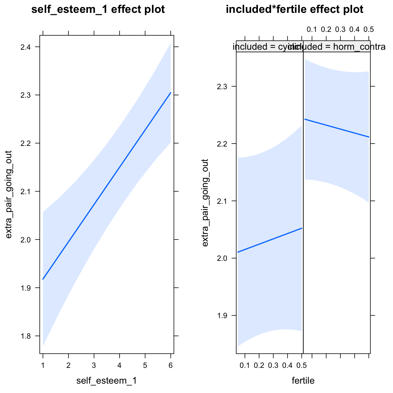
H1.1. Extra-pair going out
models$extra_pair_going_out = lmer(extra_pair_going_out ~ included * fertile + ( 1 | person), data = diary)
do_model(models$extra_pair_going_out, diary)
Narrow window
model %>%
  print_summary() %>%
  plot_all_effects()
Linear mixed model fit by REML. t-tests use Satterthwaite's method ['lmerModLmerTest']
Formula: extra_pair_going_out ~ included * fertile + (1 | person)
Data: diary
REML criterion at convergence: 22837
Scaled residuals:
Min 1Q Median 3Q Max
-2.525 -0.561 -0.179 0.361 3.463
Random effects:
Groups Name Variance Std.Dev.
person (Intercept) 0.811 0.901
Residual 1.817 1.348
Number of obs: 6378, groups: person, 493
Fixed effects:
Estimate Std. Error df t value Pr(>|t|)
(Intercept) 1.9949 0.0875 591.6244 22.81 <2e-16 ***
includedhorm_contra 0.2438 0.1038 597.7053 2.35 0.019 *
fertile 0.2388 0.1506 5982.5677 1.59 0.113
includedhorm_contra:fertile -0.3073 0.1803 5990.3304 -1.70 0.088 .
---
Signif. codes: 0 '***' 0.001 '**' 0.01 '*' 0.05 '.' 0.1 ' ' 1
Correlation of Fixed Effects:
(Intr) incld_ fertil
inclddhrm_c -0.843
fertile -0.324 0.273
inclddhrm_: 0.271 -0.327 -0.835
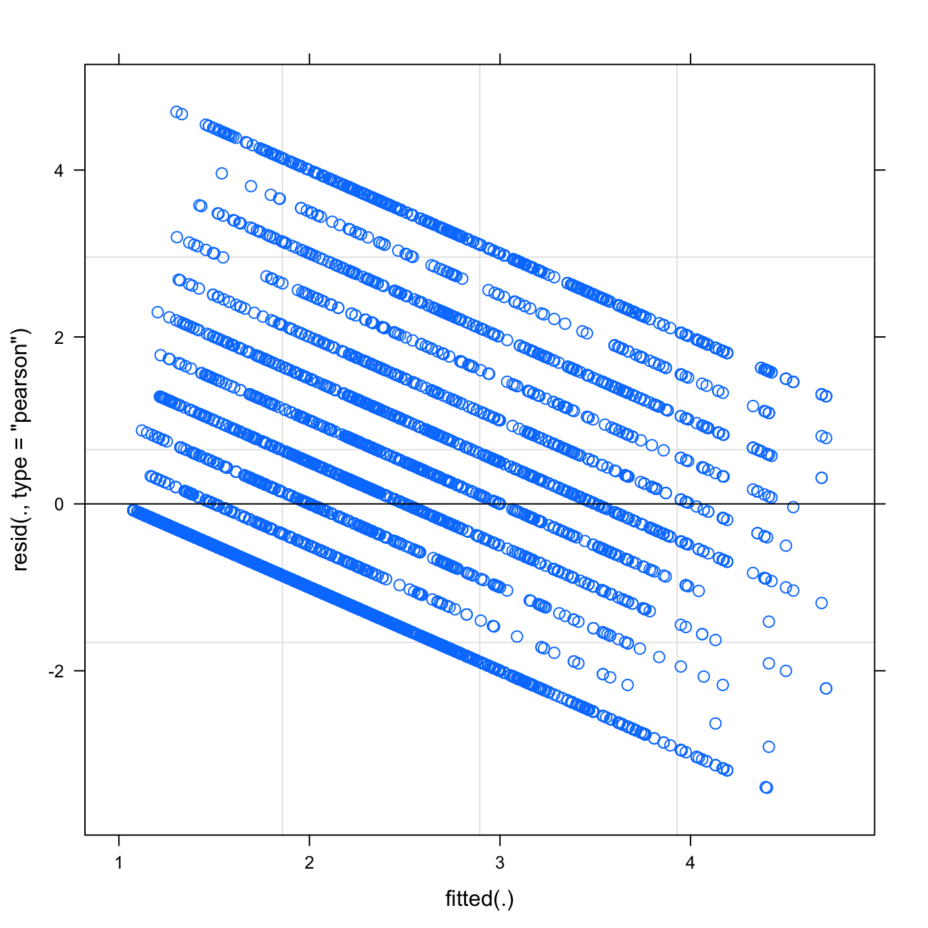
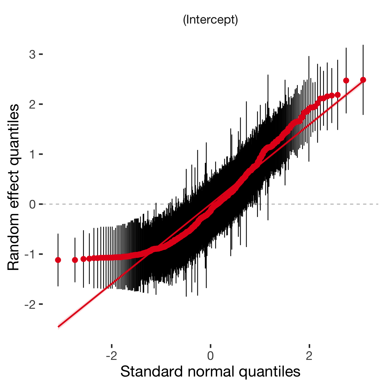
Diagnostics
model %>%
  plot_outcome(diary) %>%
  print_diagnostics()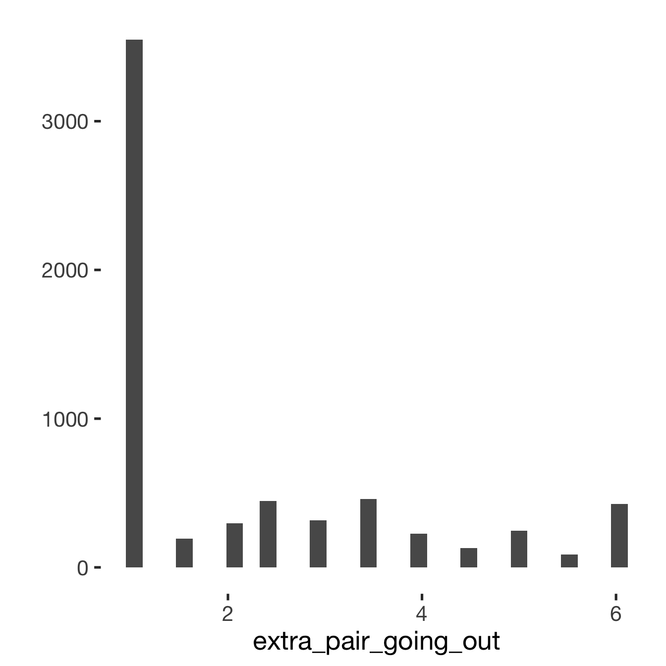
## Error in qqnorm.default(resid(obj)): y is empty or has only NAs
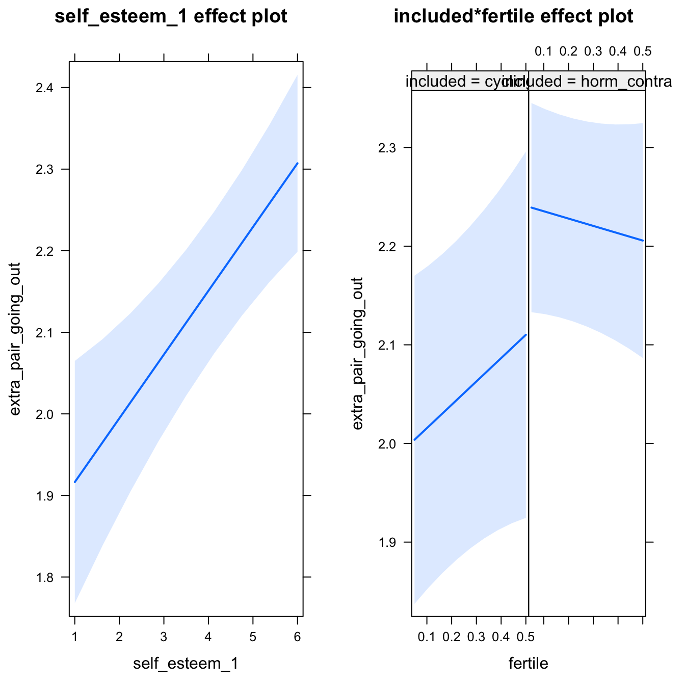
Adjusting for self esteem
model %>%
  adjust_for_self_esteem(diary)
##
##
## ```
## Linear mixed model fit by REML. t-tests use Satterthwaite's method ['lmerModLmerTest']
## Formula: form
## Data: diary
##
## REML criterion at convergence: 22827
##
## Scaled residuals:
## Min 1Q Median 3Q Max
## -2.586 -0.558 -0.189 0.367 3.494
##
## Random effects:
## Groups Name Variance Std.Dev.
## person (Intercept) 0.80 0.895
## Residual 1.81 1.347
## Number of obs: 6378, groups: person, 493
##
## Fixed effects:
## Estimate Std. Error df t value Pr(>|t|)
## (Intercept) 1.6591 0.1192 1594.1860 13.92 < 2e-16 ***
## includedhorm_contra 0.2509 0.1032 598.6683 2.43 0.015 *
## fertile 0.2365 0.1504 5982.3310 1.57 0.116
## self_esteem_1 0.0782 0.0190 6222.3613 4.12 0.000038 ***
## includedhorm_contra:fertile -0.3108 0.1801 5990.1605 -1.73 0.084 .
## ---
## Signif. codes: 0 '***' 0.001 '**' 0.01 '*' 0.05 '.' 0.1 ' ' 1
##
## Correlation of Fixed Effects:
## (Intr) incld_ fertil slf__1
## inclddhrm_c -0.627
## fertile -0.236 0.275
## self_estm_1 -0.684 0.017 -0.003
## inclddhrm_: 0.202 -0.329 -0.835 -0.005
##
## ```
Broad window
outcome = names(model@frame)[1]
broad_models[[outcome]] <<- model %>%
  switch_window_to_broad(diary)
Linear mixed model fit by REML. t-tests use Satterthwaite's method ['lmerModLmerTest']
Formula: form
Data: diary2
REML criterion at convergence: 27654
Scaled residuals:
Min 1Q Median 3Q Max
-2.511 -0.576 -0.182 0.374 3.469
Random effects:
Groups Name Variance Std.Dev.
person (Intercept) 0.791 0.889
Residual 1.834 1.354
Number of obs: 7740, groups: person, 493
Fixed effects:
Estimate Std. Error df t value Pr(>|t|)
(Intercept) 2.009 0.087 636.791 23.10 <2e-16 ***
includedhorm_contra 0.233 0.103 643.617 2.26 0.024 *
fertile 0.099 0.152 7373.402 0.65 0.514
includedhorm_contra:fertile -0.160 0.181 7383.242 -0.88 0.378
---
Signif. codes: 0 '***' 0.001 '**' 0.01 '*' 0.05 '.' 0.1 ' ' 1
Correlation of Fixed Effects:
(Intr) incld_ fertil
inclddhrm_c -0.843
fertile -0.367 0.309
inclddhrm_: 0.307 -0.371 -0.837
Diagnostics
## Warning: 'sjp.lmer' is deprecated.
## Use 'plot_model' instead.
## See help("Deprecated")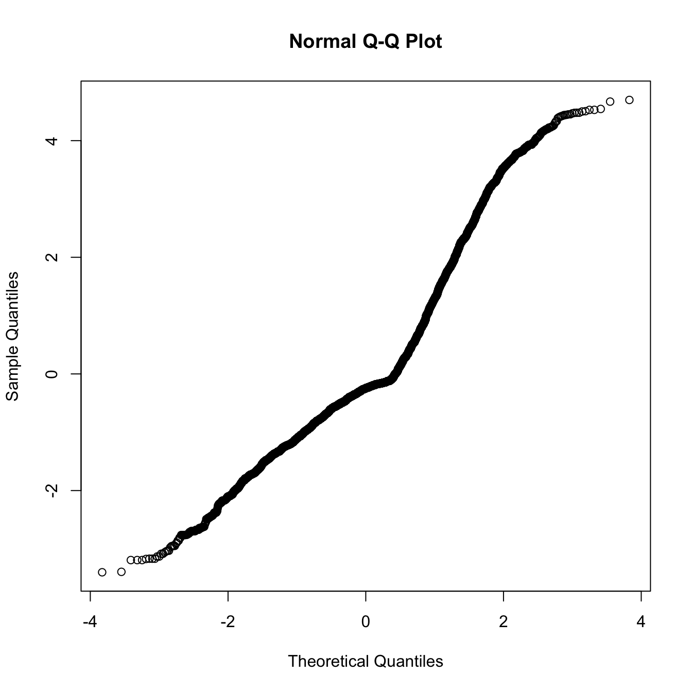
## Warning: 'sjp.lmer' is deprecated.
## Use 'plot_model' instead.
## See help("Deprecated")
Adjusting for self esteem
broad_models[[outcome]] %>%
  adjust_for_self_esteem(diary2)
##
##
## ```
## Linear mixed model fit by REML. t-tests use Satterthwaite's method ['lmerModLmerTest']
## Formula: form
## Data: diary
##
## REML criterion at convergence: 27640
##
## Scaled residuals:
## Min 1Q Median 3Q Max
## -2.537 -0.583 -0.190 0.360 3.500
##
## Random effects:
## Groups Name Variance Std.Dev.
## person (Intercept) 0.78 0.883
## Residual 1.83 1.353
## Number of obs: 7740, groups: person, 493
##
## Fixed effects:
## Estimate Std. Error df t value Pr(>|t|)
## (Intercept) 1.6763 0.1140 1575.1294 14.70 < 2e-16 ***
## includedhorm_contra 0.2401 0.1026 645.2645 2.34 0.02 *
## fertile 0.0927 0.1515 7373.6658 0.61 0.54
## self_esteem_1 0.0774 0.0173 7569.1592 4.48 0.0000077 ***
## includedhorm_contra:fertile -0.1615 0.1810 7383.3644 -0.89 0.37
## ---
## Signif. codes: 0 '***' 0.001 '**' 0.01 '*' 0.05 '.' 0.1 ' ' 1
##
## Correlation of Fixed Effects:
## (Intr) incld_ fertil slf__1
## inclddhrm_c -0.649
## fertile -0.273 0.310
## self_estm_1 -0.652 0.015 -0.009
## inclddhrm_: 0.235 -0.372 -0.837 -0.002
##
## ```
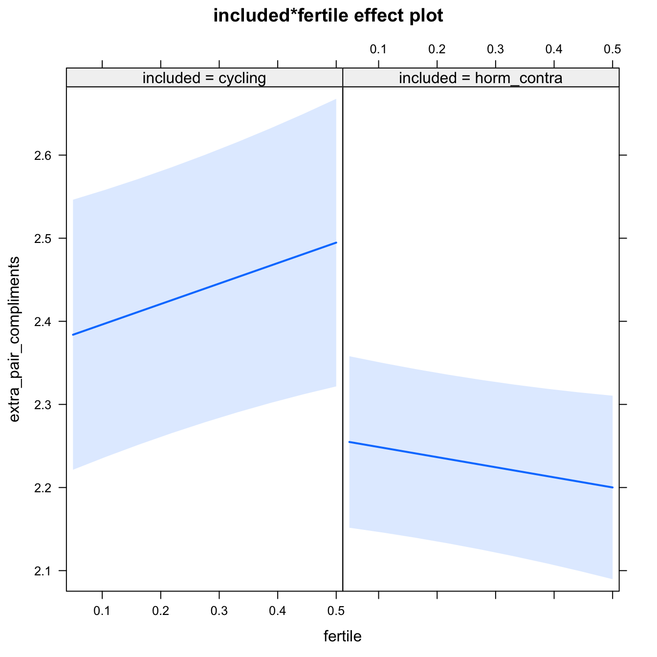
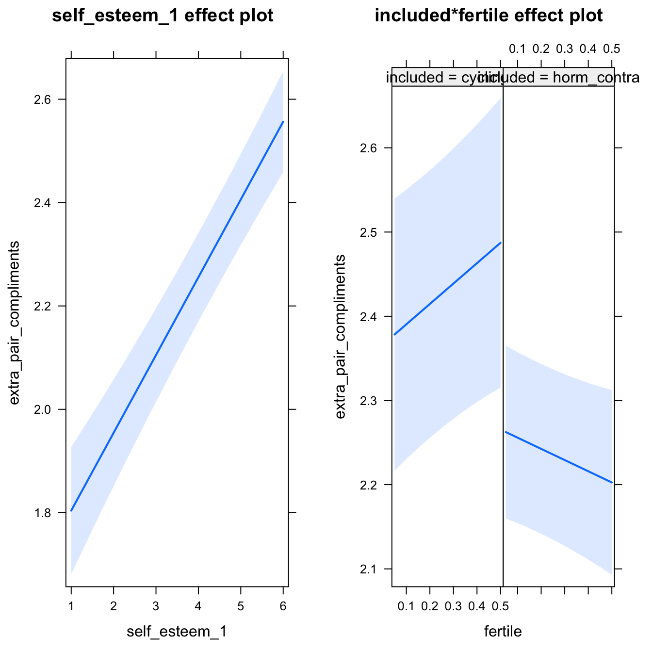
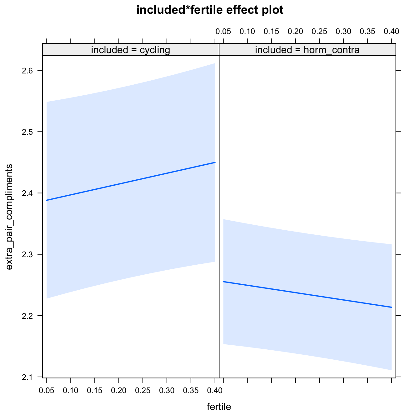
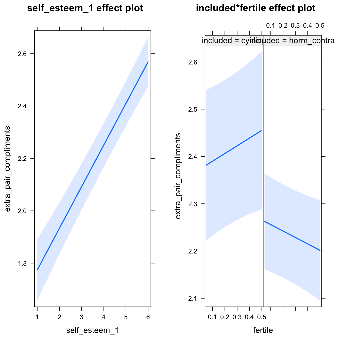
bla = 2H1.1. Extra-pair compliments
models$extra_pair_compliments = lmer(extra_pair_compliments ~ included * fertile + ( 1 | person), data = diary)
do_model(models$extra_pair_compliments, diary)
Narrow window
model %>%
  print_summary() %>%
  plot_all_effects()
Linear mixed model fit by REML. t-tests use Satterthwaite's method ['lmerModLmerTest']
Formula: extra_pair_compliments ~ included * fertile + (1 | person)
Data: diary
REML criterion at convergence: 18959
Scaled residuals:
Min 1Q Median 3Q Max
-3.777 -0.587 -0.148 0.505 4.465
Random effects:
Groups Name Variance Std.Dev.
person (Intercept) 0.854 0.924
Residual 0.943 0.971
Number of obs: 6378, groups: person, 493
Fixed effects:
Estimate Std. Error df t value Pr(>|t|)
(Intercept) 2.3715 0.0840 546.6152 28.22 <2e-16 ***
includedhorm_contra -0.1106 0.0996 549.6377 -1.11 0.2670
fertile 0.2464 0.1087 5943.2303 2.27 0.0235 *
includedhorm_contra:fertile -0.3679 0.1301 5947.3329 -2.83 0.0047 **
---
Signif. codes: 0 '***' 0.001 '**' 0.01 '*' 0.05 '.' 0.1 ' ' 1
Correlation of Fixed Effects:
(Intr) incld_ fertil
inclddhrm_c -0.844
fertile -0.244 0.206
inclddhrm_: 0.203 -0.246 -0.835
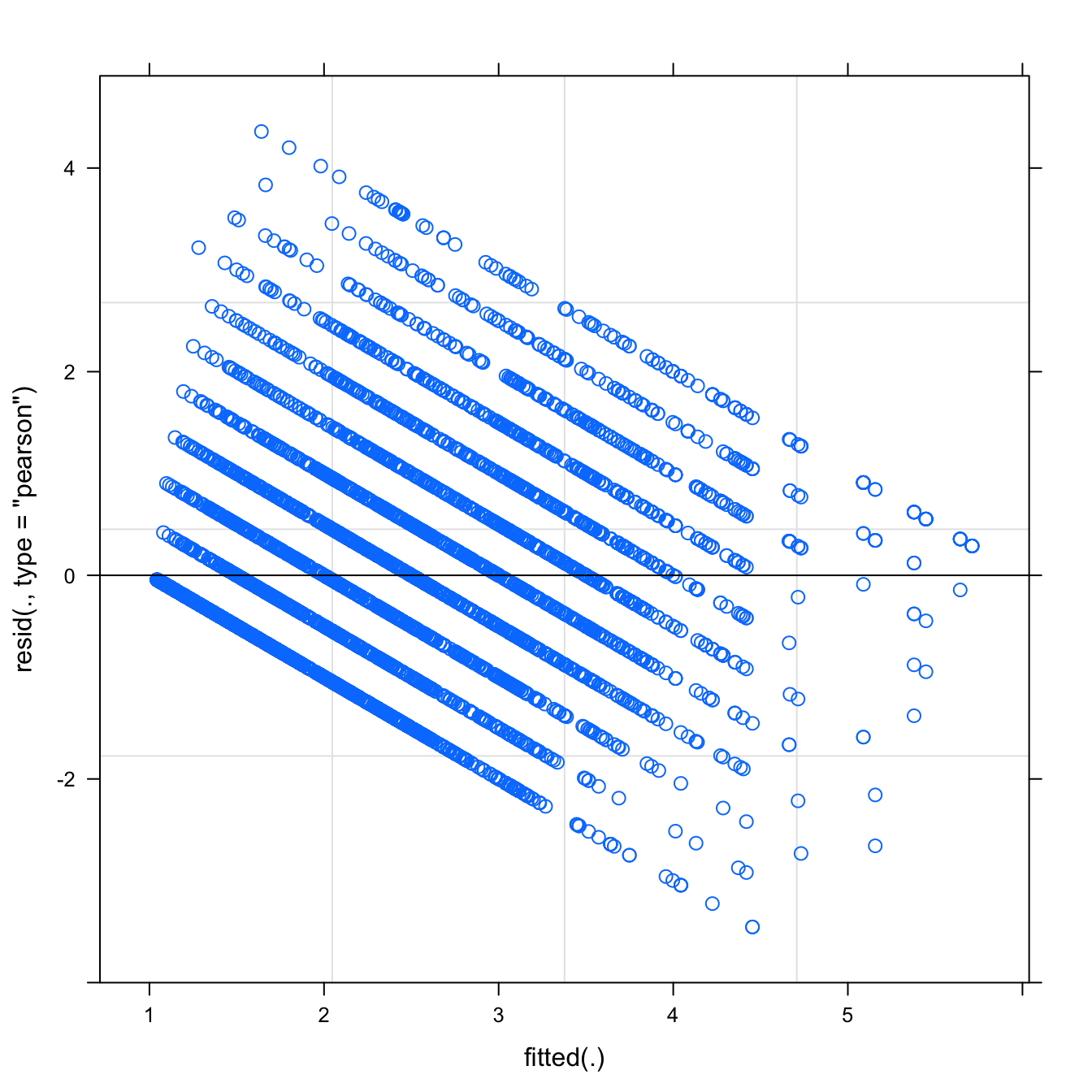
Diagnostics
model %>%
  plot_outcome(diary) %>%
  print_diagnostics()
## Error in qqnorm.default(resid(obj)): y is empty or has only NAs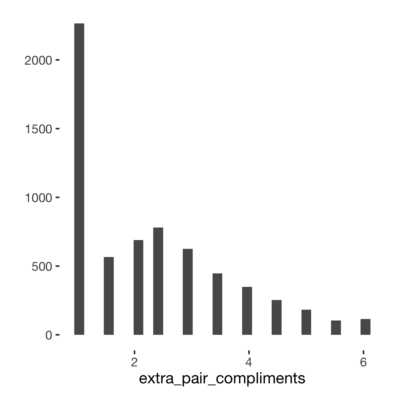
Adjusting for self esteem
model %>%
  adjust_for_self_esteem(diary)
##
##
## ```
## Linear mixed model fit by REML. t-tests use Satterthwaite's method ['lmerModLmerTest']
## Formula: form
## Data: diary
##
## REML criterion at convergence: 18850
##
## Scaled residuals:
## Min 1Q Median 3Q Max
## -3.701 -0.591 -0.150 0.509 4.595
##
## Random effects:
## Groups Name Variance Std.Dev.
## person (Intercept) 0.844 0.919
## Residual 0.925 0.962
## Number of obs: 6378, groups: person, 493
##
## Fixed effects:
## Estimate Std. Error df t value Pr(>|t|)
## (Intercept) 1.7252 0.1027 1140.8433 16.79 <2e-16 ***
## includedhorm_contra -0.0971 0.0989 549.0000 -0.98 0.3267
## fertile 0.2421 0.1077 5941.7046 2.25 0.0246 *
## self_esteem_1 0.1505 0.0139 6361.9150 10.80 <2e-16 ***
## includedhorm_contra:fertile -0.3750 0.1290 5945.7700 -2.91 0.0037 **
## ---
## Signif. codes: 0 '***' 0.001 '**' 0.01 '*' 0.05 '.' 0.1 ' ' 1
##
## Correlation of Fixed Effects:
## (Intr) incld_ fertil slf__1
## inclddhrm_c -0.693
## fertile -0.195 0.205
## self_estm_1 -0.583 0.013 -0.004
## inclddhrm_: 0.168 -0.245 -0.835 -0.005
##
## ```
Broad window
outcome = names(model@frame)[1]
broad_models[[outcome]] <<- model %>%
  switch_window_to_broad(diary)
Linear mixed model fit by REML. t-tests use Satterthwaite's method ['lmerModLmerTest']
Formula: form
Data: diary2
REML criterion at convergence: 22877
Scaled residuals:
Min 1Q Median 3Q Max
-3.542 -0.585 -0.143 0.498 4.470
Random effects:
Groups Name Variance Std.Dev.
person (Intercept) 0.830 0.911
Residual 0.951 0.975
Number of obs: 7740, groups: person, 493
Fixed effects:
Estimate Std. Error df t value Pr(>|t|)
(Intercept) 2.3793 0.0832 568.9740 28.61 <2e-16 ***
includedhorm_contra -0.1179 0.0986 572.2982 -1.20 0.232
fertile 0.1762 0.1094 7322.6186 1.61 0.107
includedhorm_contra:fertile -0.2958 0.1307 7328.3508 -2.26 0.024 *
---
Signif. codes: 0 '***' 0.001 '**' 0.01 '*' 0.05 '.' 0.1 ' ' 1
Correlation of Fixed Effects:
(Intr) incld_ fertil
inclddhrm_c -0.844
fertile -0.276 0.233
inclddhrm_: 0.231 -0.279 -0.837
Diagnostics
## Warning: 'sjp.lmer' is deprecated.
## Use 'plot_model' instead.
## See help("Deprecated")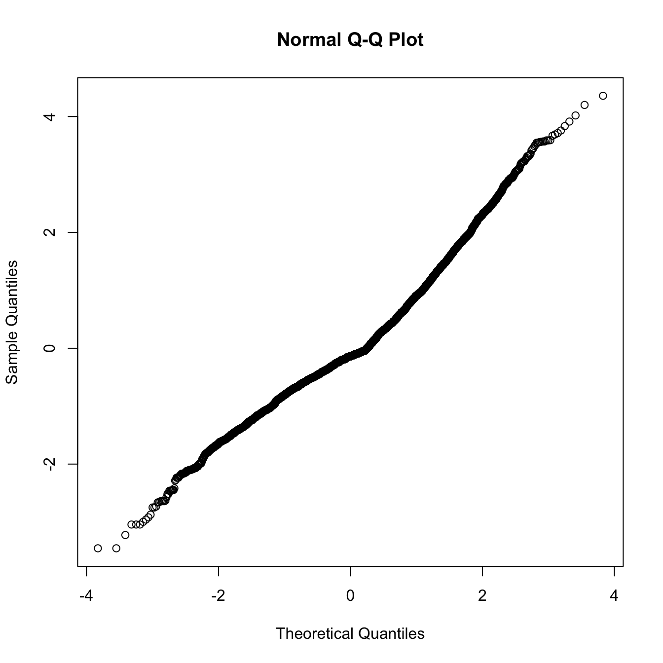
## Warning: 'sjp.lmer' is deprecated.
## Use 'plot_model' instead.
## See help("Deprecated")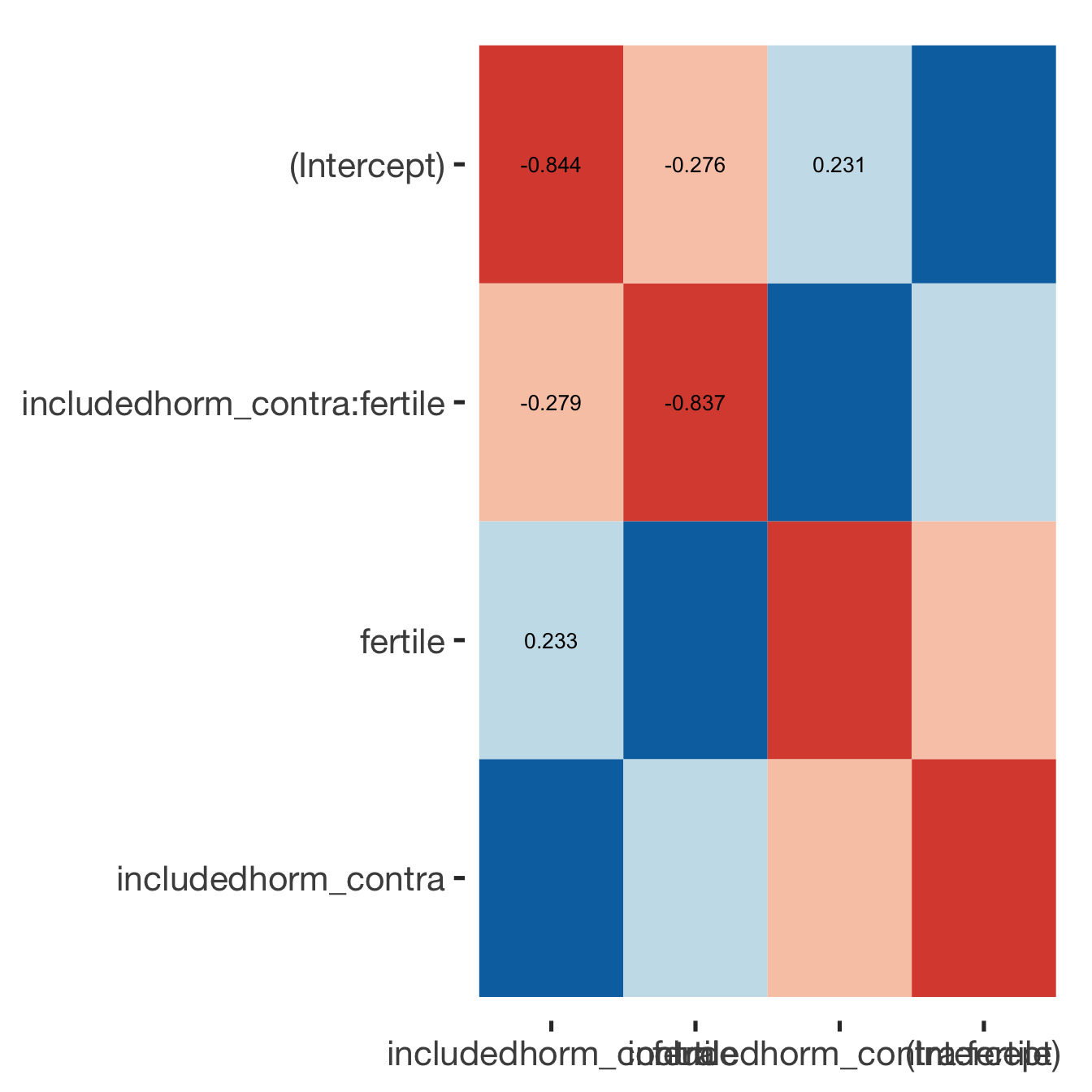
Adjusting for self esteem
broad_models[[outcome]] %>%
  adjust_for_self_esteem(diary2)
##
##
## ```
## Linear mixed model fit by REML. t-tests use Satterthwaite's method ['lmerModLmerTest']
## Formula: form
## Data: diary
##
## REML criterion at convergence: 22727
##
## Scaled residuals:
## Min 1Q Median 3Q Max
## -3.488 -0.588 -0.144 0.521 4.522
##
## Random effects:
## Groups Name Variance Std.Dev.
## person (Intercept) 0.818 0.904
## Residual 0.931 0.965
## Number of obs: 7740, groups: person, 493
##
## Fixed effects:
## Estimate Std. Error df t value Pr(>|t|)
## (Intercept) 1.6969 0.0988 1091.7657 17.18 <2e-16 ***
## includedhorm_contra -0.1040 0.0978 571.5931 -1.06 0.288
## fertile 0.1632 0.1083 7321.2055 1.51 0.132
## self_esteem_1 0.1589 0.0126 7724.0676 12.58 <2e-16 ***
## includedhorm_contra:fertile -0.2994 0.1294 7326.7544 -2.31 0.021 *
## ---
## Signif. codes: 0 '***' 0.001 '**' 0.01 '*' 0.05 '.' 0.1 ' ' 1
##
## Correlation of Fixed Effects:
## (Intr) incld_ fertil slf__1
## inclddhrm_c -0.711
## fertile -0.225 0.232
## self_estm_1 -0.549 0.011 -0.010
## inclddhrm_: 0.194 -0.279 -0.837 -0.002
##
## ```
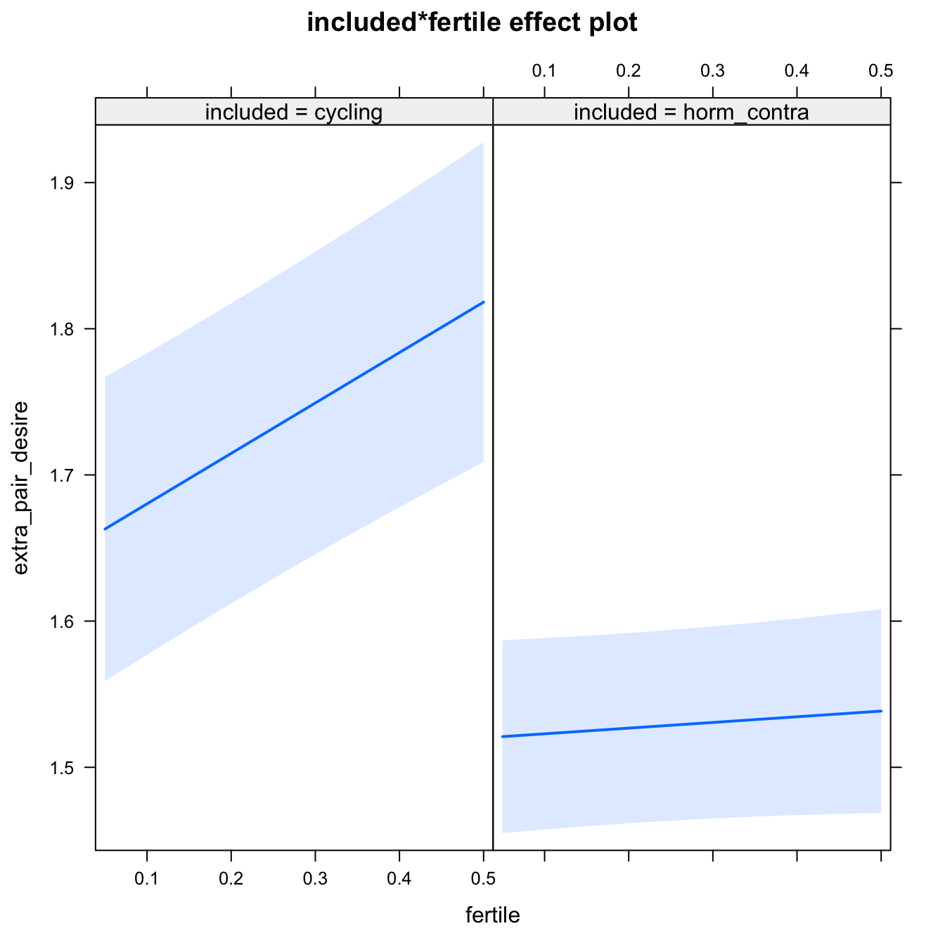
bla = 2H1.1. Extra-pair desire
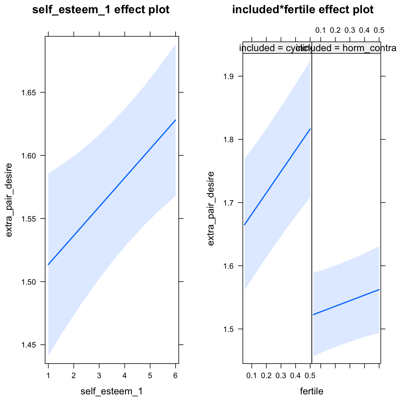
models$extra_pair_desire = lmer(extra_pair_desire ~ included * fertile + ( 1 | person), data = diary)
do_model(models$extra_pair_desire, diary)
Narrow window
model %>%
  print_summary() %>%
  plot_all_effects()
Linear mixed model fit by REML. t-tests use Satterthwaite's method ['lmerModLmerTest']
Formula: extra_pair_desire ~ included * fertile + (1 | person)
Data: diary
REML criterion at convergence: 11989
Scaled residuals:
Min 1Q Median 3Q Max
-5.651 -0.464 -0.137 0.341 6.554
Random effects:
Groups Name Variance Std.Dev.
person (Intercept) 0.359 0.599
Residual 0.310 0.557
Number of obs: 6378, groups: person, 493
Fixed effects:
Estimate Std. Error df t value Pr(>|t|)
(Intercept) 1.6457 0.0536 536.5494 30.69 < 2e-16 ***
includedhorm_contra -0.1267 0.0635 538.9024 -1.99 0.047 *
fertile 0.3450 0.0624 5933.4257 5.53 0.000000034 ***
includedhorm_contra:fertile -0.3062 0.0747 5936.6353 -4.10 0.000042520 ***
---
Signif. codes: 0 '***' 0.001 '**' 0.01 '*' 0.05 '.' 0.1 ' ' 1
Correlation of Fixed Effects:
(Intr) incld_ fertil
inclddhrm_c -0.844
fertile -0.219 0.185
inclddhrm_: 0.183 -0.221 -0.835
Diagnostics
model %>%
  plot_outcome(diary) %>%
  print_diagnostics()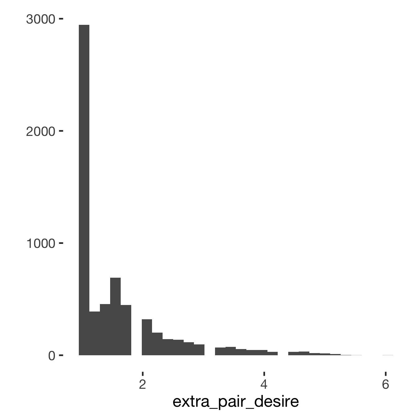
## Error in qqnorm.default(resid(obj)): y is empty or has only NAs
Adjusting for self esteem
model %>%
  adjust_for_self_esteem(diary)
##
##
## ```
## Linear mixed model fit by REML. t-tests use Satterthwaite's method ['lmerModLmerTest']
## Formula: form
## Data: diary
##
## REML criterion at convergence: 11992
##
## Scaled residuals:
## Min 1Q Median 3Q Max
## -5.619 -0.466 -0.137 0.340 6.491
##
## Random effects:
## Groups Name Variance Std.Dev.
## person (Intercept) 0.36 0.600
## Residual 0.31 0.557
## Number of obs: 6378, groups: person, 493
##
## Fixed effects:
## Estimate Std. Error df t value Pr(>|t|)
## (Intercept) 1.56762 0.06402 1019.03265 24.49 < 2e-16 ***
## includedhorm_contra -0.12506 0.06360 538.75595 -1.97 0.050 *
## fertile 0.34446 0.06239 5932.29881 5.52 0.000000035 ***
## self_esteem_1 0.01819 0.00812 6323.72882 2.24 0.025 *
## includedhorm_contra:fertile -0.30701 0.07471 5935.48171 -4.11 0.000040163 ***
## ---
## Signif. codes: 0 '***' 0.001 '**' 0.01 '*' 0.05 '.' 0.1 ' ' 1
##
## Correlation of Fixed Effects:
## (Intr) incld_ fertil slf__1
## inclddhrm_c -0.714
## fertile -0.181 0.185
## self_estm_1 -0.545 0.011 -0.004
## inclddhrm_: 0.156 -0.221 -0.835 -0.005
##
## ```
Broad window
outcome = names(model@frame)[1]
broad_models[[outcome]] <<- model %>%
  switch_window_to_broad(diary)
Linear mixed model fit by REML. t-tests use Satterthwaite's method ['lmerModLmerTest']
Formula: form
Data: diary2
REML criterion at convergence: 14579
Scaled residuals:
Min 1Q Median 3Q Max
-5.287 -0.494 -0.136 0.336 6.879
Random effects:
Groups Name Variance Std.Dev.
person (Intercept) 0.355 0.595
Residual 0.321 0.566
Number of obs: 7740, groups: person, 493
Fixed effects:
Estimate Std. Error df t value Pr(>|t|)
(Intercept) 1.6489 0.0535 554.2481 30.81 < 2e-16 ***
includedhorm_contra -0.1317 0.0634 556.8428 -2.08 0.0382 *
fertile 0.3385 0.0636 7309.8904 5.32 0.00000011 ***
includedhorm_contra:fertile -0.2484 0.0760 7314.5718 -3.27 0.0011 **
---
Signif. codes: 0 '***' 0.001 '**' 0.01 '*' 0.05 '.' 0.1 ' ' 1
Correlation of Fixed Effects:
(Intr) incld_ fertil
inclddhrm_c -0.844
fertile -0.249 0.210
inclddhrm_: 0.208 -0.252 -0.837
Diagnostics
## Warning: 'sjp.lmer' is deprecated.
## Use 'plot_model' instead.
## See help("Deprecated")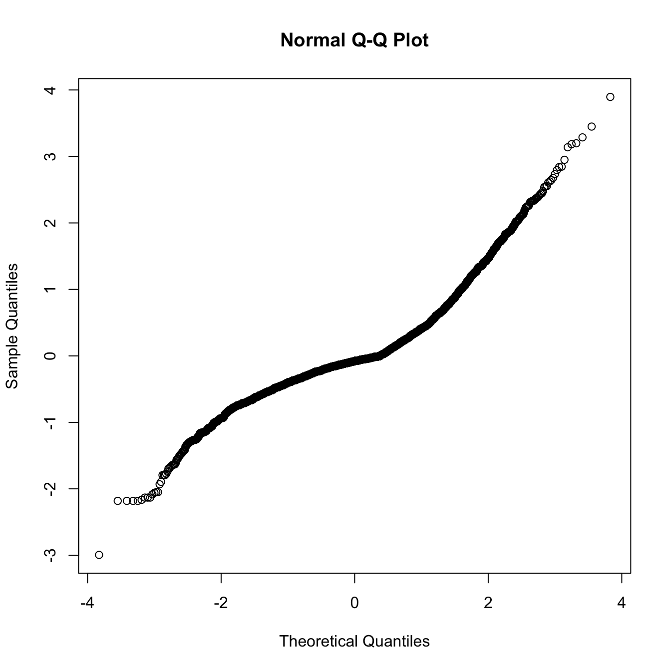
## Warning: 'sjp.lmer' is deprecated.
## Use 'plot_model' instead.
## See help("Deprecated")
Adjusting for self esteem
broad_models[[outcome]] %>%
  adjust_for_self_esteem(diary2)
##
##
## ```
## Linear mixed model fit by REML. t-tests use Satterthwaite's method ['lmerModLmerTest']
## Formula: form
## Data: diary
##
## REML criterion at convergence: 14578
##
## Scaled residuals:
## Min 1Q Median 3Q Max
## -5.257 -0.490 -0.138 0.342 6.802
##
## Random effects:
## Groups Name Variance Std.Dev.
## person (Intercept) 0.356 0.596
## Residual 0.320 0.566
## Number of obs: 7740, groups: person, 493
##
## Fixed effects:
## Estimate Std. Error df t value Pr(>|t|)
## (Intercept) 1.55063 0.06241 975.03261 24.85 < 2e-16 ***
## includedhorm_contra -0.12973 0.06349 556.52197 -2.04 0.0415 *
## fertile 0.33667 0.06356 7308.73362 5.30 0.00000012 ***
## self_esteem_1 0.02289 0.00745 7686.31248 3.07 0.0021 **
## includedhorm_contra:fertile -0.24888 0.07594 7313.26024 -3.28 0.0011 **
## ---
## Signif. codes: 0 '***' 0.001 '**' 0.01 '*' 0.05 '.' 0.1 ' ' 1
##
## Correlation of Fixed Effects:
## (Intr) incld_ fertil slf__1
## inclddhrm_c -0.730
## fertile -0.208 0.210
## self_estm_1 -0.512 0.010 -0.010
## inclddhrm_: 0.180 -0.252 -0.837 -0.002
##
## ```
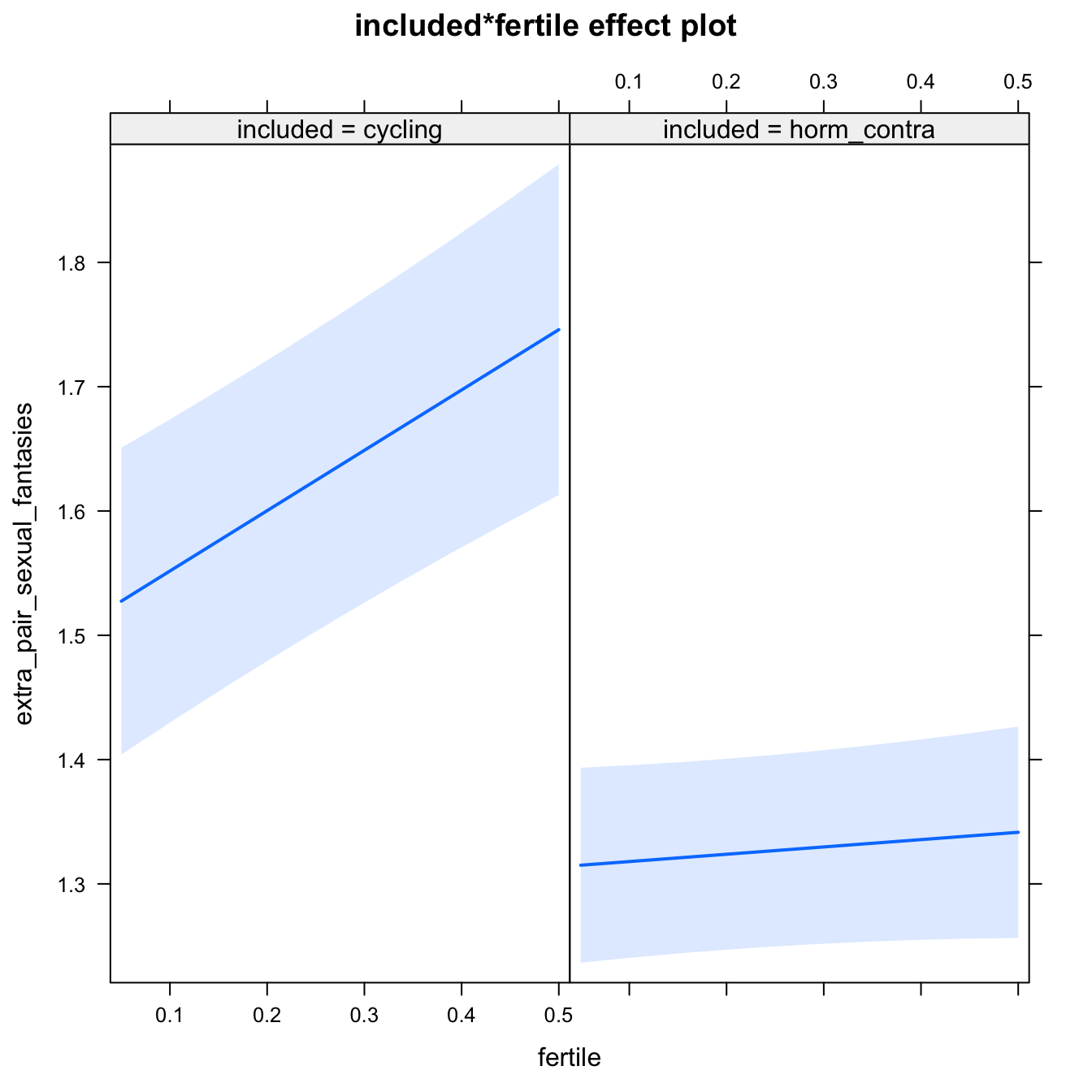
bla = 2H1.1. Extra-pair sexual fantasies
models$extra_pair_sexual_fantasies = lmer(extra_pair_sexual_fantasies ~ included * fertile + ( 1 | person), data = diary)
do_model(models$extra_pair_sexual_fantasies, diary)
Narrow window
model %>%
  print_summary() %>%
  plot_all_effects()
Linear mixed model fit by REML. t-tests use Satterthwaite's method ['lmerModLmerTest']
Formula: extra_pair_sexual_fantasies ~ included * fertile + (1 | person)
Data: diary
REML criterion at convergence: 16616
Scaled residuals:
Min 1Q Median 3Q Max
-4.492 -0.309 -0.059 -0.021 5.814
Random effects:
Groups Name Variance Std.Dev.
person (Intercept) 0.479 0.692
Residual 0.663 0.814
Number of obs: 6378, groups: person, 493
Fixed effects:
Estimate Std. Error df t value Pr(>|t|)
(Intercept) 1.5032 0.0640 555.0510 23.49 < 2e-16 ***
includedhorm_contra -0.1911 0.0759 558.8408 -2.52 0.012 *
fertile 0.4855 0.0911 5951.5584 5.33 0.0000001 ***
includedhorm_contra:fertile -0.4266 0.1091 5956.6984 -3.91 0.0000930 ***
---
Signif. codes: 0 '***' 0.001 '**' 0.01 '*' 0.05 '.' 0.1 ' ' 1
Correlation of Fixed Effects:
(Intr) incld_ fertil
inclddhrm_c -0.844
fertile -0.268 0.226
inclddhrm_: 0.224 -0.271 -0.835
Diagnostics
model %>%
  plot_outcome(diary) %>%
  print_diagnostics()
## Error in qqnorm.default(resid(obj)): y is empty or has only NAs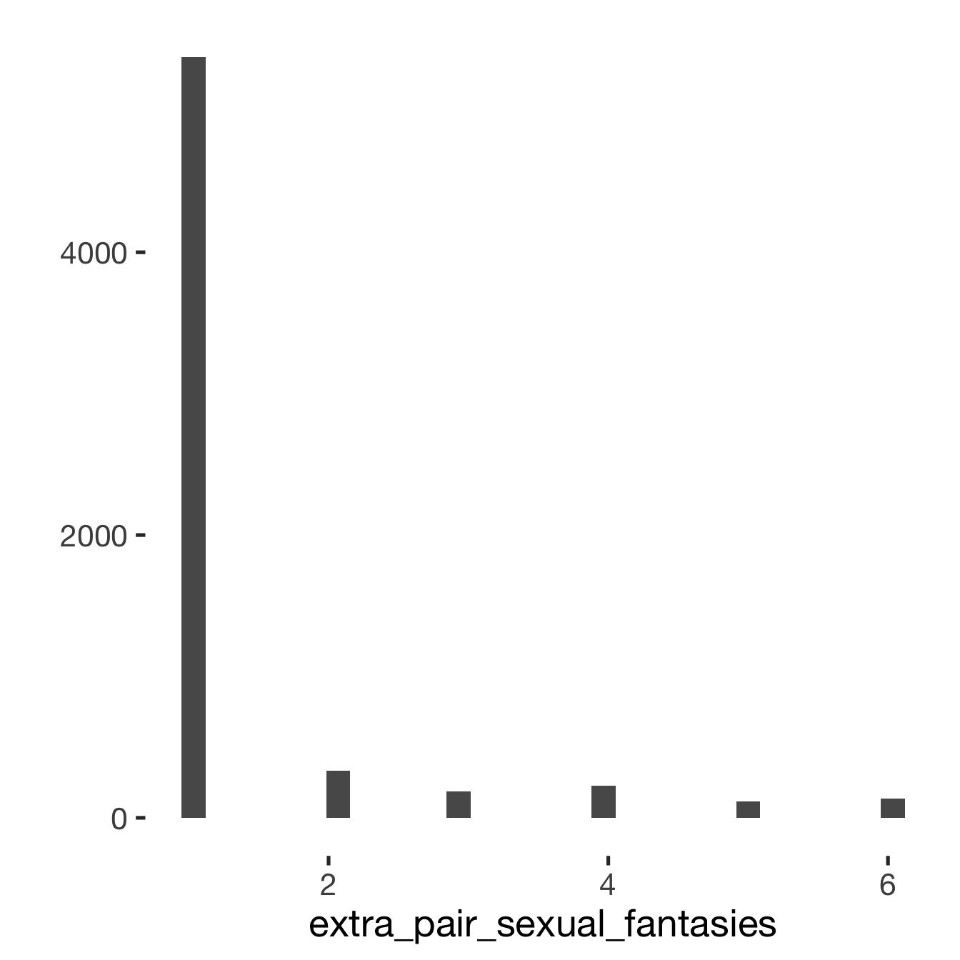
Adjusting for self esteem
model %>%
  adjust_for_self_esteem(diary)
##
##
## ```
## Linear mixed model fit by REML. t-tests use Satterthwaite's method ['lmerModLmerTest']
## Formula: form
## Data: diary
##
## REML criterion at convergence: 16619
##
## Scaled residuals:
## Min 1Q Median 3Q Max
## -4.467 -0.306 -0.063 -0.013 5.833
##
## Random effects:
## Groups Name Variance Std.Dev.
## person (Intercept) 0.481 0.694
## Residual 0.663 0.814
## Number of obs: 6378, groups: person, 493
##
## Fixed effects:
## Estimate Std. Error df t value Pr(>|t|)
## (Intercept) 1.4050 0.0815 1266.4108 17.24 < 2e-16 ***
## includedhorm_contra -0.1891 0.0760 557.9803 -2.49 0.013 *
## fertile 0.4848 0.0911 5949.8760 5.32 0.00000011 ***
## self_esteem_1 0.0229 0.0117 6372.2727 1.95 0.051 .
## includedhorm_contra:fertile -0.4277 0.1090 5954.9766 -3.92 0.00008883 ***
## ---
## Signif. codes: 0 '***' 0.001 '**' 0.01 '*' 0.05 '.' 0.1 ' ' 1
##
## Correlation of Fixed Effects:
## (Intr) incld_ fertil slf__1
## inclddhrm_c -0.672
## fertile -0.208 0.226
## self_estm_1 -0.617 0.014 -0.004
## inclddhrm_: 0.179 -0.270 -0.835 -0.005
##
## ```
Broad window
outcome = names(model@frame)[1]
broad_models[[outcome]] <<- model %>%
  switch_window_to_broad(diary)
Linear mixed model fit by REML. t-tests use Satterthwaite's method ['lmerModLmerTest']
Formula: form
Data: diary2
REML criterion at convergence: 20305
Scaled residuals:
Min 1Q Median 3Q Max
-4.501 -0.319 -0.070 -0.003 5.759
Random effects:
Groups Name Variance Std.Dev.
person (Intercept) 0.475 0.689
Residual 0.691 0.831
Number of obs: 7740, groups: person, 493
Fixed effects:
Estimate Std. Error df t value Pr(>|t|)
(Intercept) 1.5066 0.0641 582.7504 23.49 < 2e-16 ***
includedhorm_contra -0.1985 0.0760 586.9808 -2.61 0.0093 **
fertile 0.4625 0.0933 7334.3196 4.96 0.00000072 ***
includedhorm_contra:fertile -0.3275 0.1114 7341.3419 -2.94 0.0033 **
---
Signif. codes: 0 '***' 0.001 '**' 0.01 '*' 0.05 '.' 0.1 ' ' 1
Correlation of Fixed Effects:
(Intr) incld_ fertil
inclddhrm_c -0.844
fertile -0.305 0.257
inclddhrm_: 0.255 -0.309 -0.837
Diagnostics
## Warning: 'sjp.lmer' is deprecated.
## Use 'plot_model' instead.
## See help("Deprecated")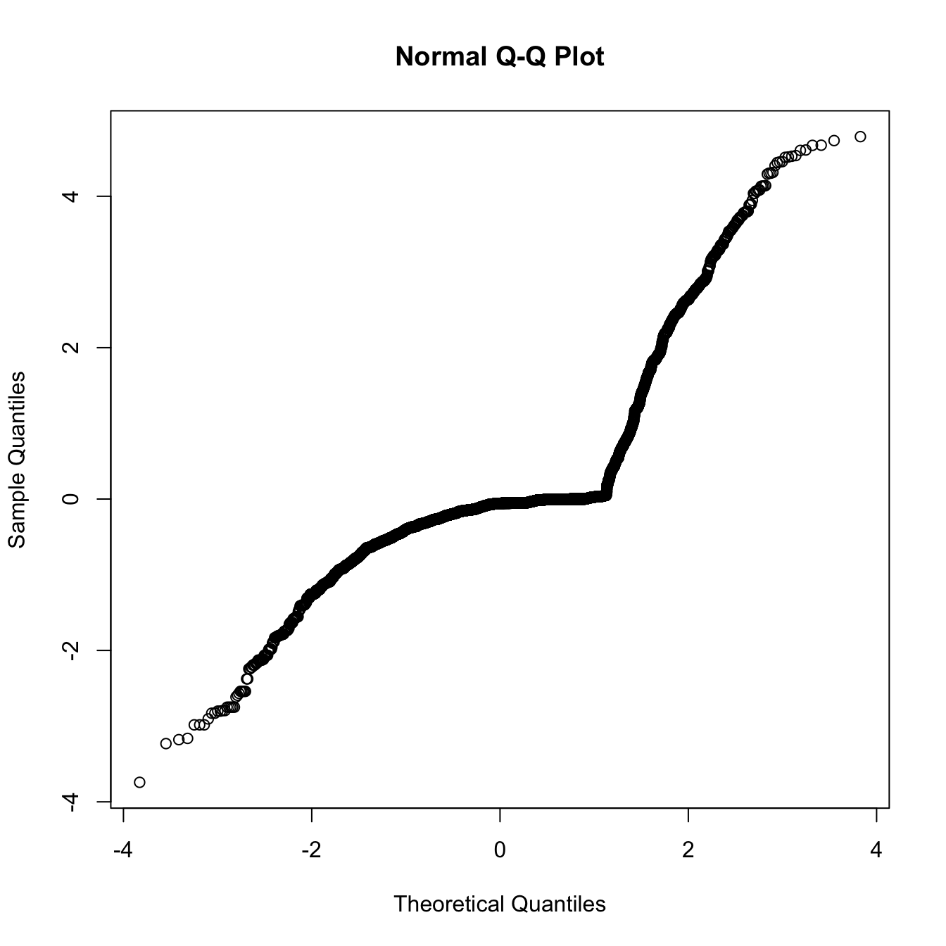
## Warning: 'sjp.lmer' is deprecated.
## Use 'plot_model' instead.
## See help("Deprecated")
Adjusting for self esteem
broad_models[[outcome]] %>%
  adjust_for_self_esteem(diary2)
##
##
## ```
## Linear mixed model fit by REML. t-tests use Satterthwaite's method ['lmerModLmerTest']
## Formula: form
## Data: diary
##
## REML criterion at convergence: 20307
##
## Scaled residuals:
## Min 1Q Median 3Q Max
## -4.481 -0.319 -0.080 -0.004 5.741
##
## Random effects:
## Groups Name Variance Std.Dev.
## person (Intercept) 0.478 0.692
## Residual 0.690 0.831
## Number of obs: 7740, groups: person, 493
##
## Fixed effects:
## Estimate Std. Error df t value Pr(>|t|)
## (Intercept) 1.3953 0.0793 1222.2011 17.59 < 2e-16 ***
## includedhorm_contra -0.1963 0.0762 585.7570 -2.57 0.0103 *
## fertile 0.4604 0.0932 7332.5814 4.94 0.0000008 ***
## self_esteem_1 0.0259 0.0108 7733.6131 2.40 0.0165 *
## includedhorm_contra:fertile -0.3281 0.1114 7339.3869 -2.95 0.0032 **
## ---
## Signif. codes: 0 '***' 0.001 '**' 0.01 '*' 0.05 '.' 0.1 ' ' 1
##
## Correlation of Fixed Effects:
## (Intr) incld_ fertil slf__1
## inclddhrm_c -0.691
## fertile -0.241 0.256
## self_estm_1 -0.585 0.012 -0.009
## inclddhrm_: 0.208 -0.308 -0.837 -0.002
##
## ```
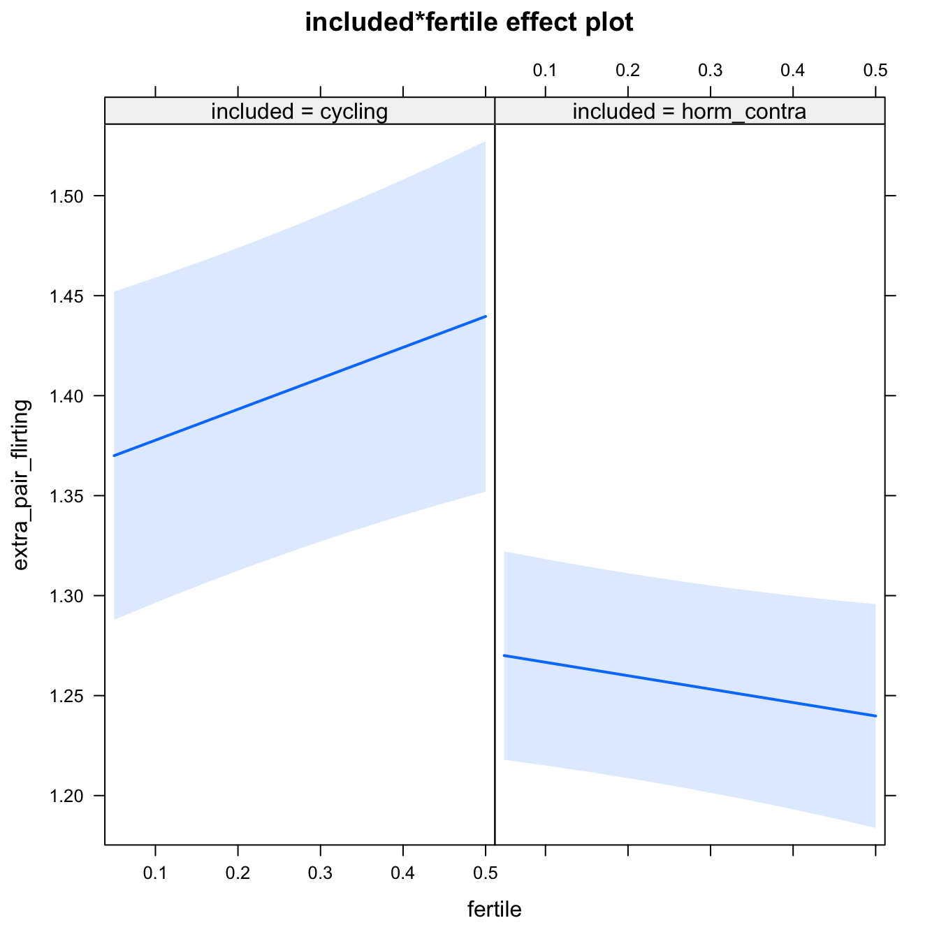
bla = 2H1.1. Extra-pair flirting
models$extra_pair_flirting = lmer(extra_pair_flirting ~ included * fertile + ( 1 | person), data = diary)
do_model(models$extra_pair_flirting, diary)
Narrow window
model %>%
  print_summary() %>%
  plot_all_effects()
Linear mixed model fit by REML. t-tests use Satterthwaite's method ['lmerModLmerTest']
Formula: extra_pair_flirting ~ included * fertile + (1 | person)
Data: diary
REML criterion at convergence: 10488
Scaled residuals:
Min 1Q Median 3Q Max
-4.601 -0.325 -0.084 -0.008 8.721
Random effects:
Groups Name Variance Std.Dev.
person (Intercept) 0.217 0.466
Residual 0.250 0.500
Number of obs: 6378, groups: person, 493
Fixed effects:
Estimate Std. Error df t value Pr(>|t|)
(Intercept) 1.3623 0.0425 549.8936 32.07 < 2e-16 ***
includedhorm_contra -0.0889 0.0503 553.0644 -1.77 0.07807 .
fertile 0.1547 0.0560 5946.1599 2.76 0.00575 **
includedhorm_contra:fertile -0.2219 0.0671 5950.4397 -3.31 0.00094 ***
---
Signif. codes: 0 '***' 0.001 '**' 0.01 '*' 0.05 '.' 0.1 ' ' 1
Correlation of Fixed Effects:
(Intr) incld_ fertil
inclddhrm_c -0.844
fertile -0.248 0.210
inclddhrm_: 0.207 -0.251 -0.835
Diagnostics
model %>%
  plot_outcome(diary) %>%
  print_diagnostics()
## Error in qqnorm.default(resid(obj)): y is empty or has only NAs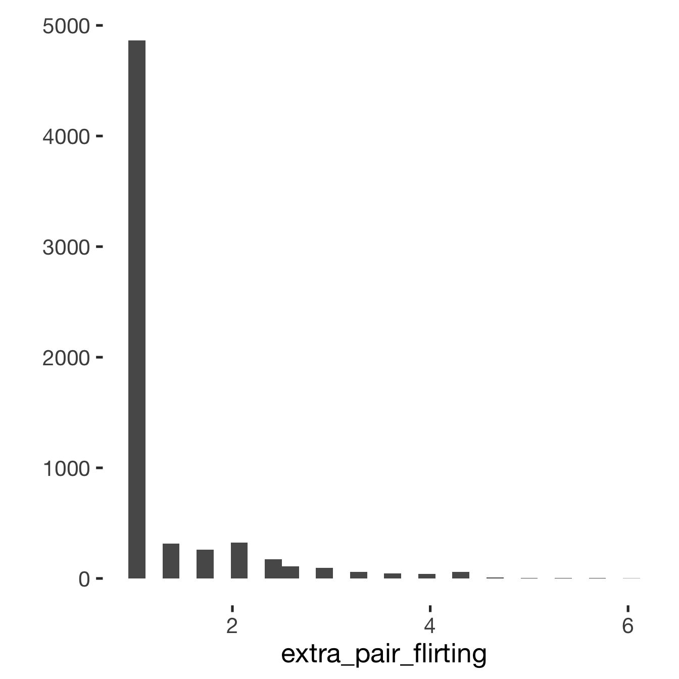
Adjusting for self esteem
model %>%
  adjust_for_self_esteem(diary)
##
##
## ```
## Linear mixed model fit by REML. t-tests use Satterthwaite's method ['lmerModLmerTest']
## Formula: form
## Data: diary
##
## REML criterion at convergence: 10489
##
## Scaled residuals:
## Min 1Q Median 3Q Max
## -4.592 -0.330 -0.095 -0.006 8.651
##
## Random effects:
## Groups Name Variance Std.Dev.
## person (Intercept) 0.217 0.466
## Residual 0.250 0.500
## Number of obs: 6378, groups: person, 493
##
## Fixed effects:
## Estimate Std. Error df t value Pr(>|t|)
## (Intercept) 1.28143 0.05266 1169.93469 24.33 < 2e-16 ***
## includedhorm_contra -0.08717 0.05039 552.81241 -1.73 0.08419 .
## fertile 0.15420 0.05598 5944.95729 2.75 0.00589 **
## self_esteem_1 0.01882 0.00724 6366.69858 2.60 0.00931 **
## includedhorm_contra:fertile -0.22277 0.06703 5949.20805 -3.32 0.00089 ***
## ---
## Signif. codes: 0 '***' 0.001 '**' 0.01 '*' 0.05 '.' 0.1 ' ' 1
##
## Correlation of Fixed Effects:
## (Intr) incld_ fertil slf__1
## inclddhrm_c -0.689
## fertile -0.198 0.209
## self_estm_1 -0.590 0.013 -0.004
## inclddhrm_: 0.170 -0.250 -0.835 -0.005
##
## ```
Broad window
outcome = names(model@frame)[1]
broad_models[[outcome]] <<- model %>%
  switch_window_to_broad(diary)
Linear mixed model fit by REML. t-tests use Satterthwaite's method ['lmerModLmerTest']
Formula: form
Data: diary2
REML criterion at convergence: 12526
Scaled residuals:
Min 1Q Median 3Q Max
-4.796 -0.351 -0.100 -0.013 8.983
Random effects:
Groups Name Variance Std.Dev.
person (Intercept) 0.214 0.463
Residual 0.250 0.500
Number of obs: 7740, groups: person, 493
Fixed effects:
Estimate Std. Error df t value Pr(>|t|)
(Intercept) 1.3660 0.0423 569.0738 32.28 <2e-16 ***
includedhorm_contra -0.0942 0.0502 572.4492 -1.88 0.0610 .
fertile 0.1339 0.0561 7322.8023 2.39 0.0169 *
includedhorm_contra:fertile -0.1861 0.0670 7328.6230 -2.78 0.0055 **
---
Signif. codes: 0 '***' 0.001 '**' 0.01 '*' 0.05 '.' 0.1 ' ' 1
Correlation of Fixed Effects:
(Intr) incld_ fertil
inclddhrm_c -0.844
fertile -0.278 0.234
inclddhrm_: 0.233 -0.281 -0.837
Diagnostics
## Warning: 'sjp.lmer' is deprecated.
## Use 'plot_model' instead.
## See help("Deprecated")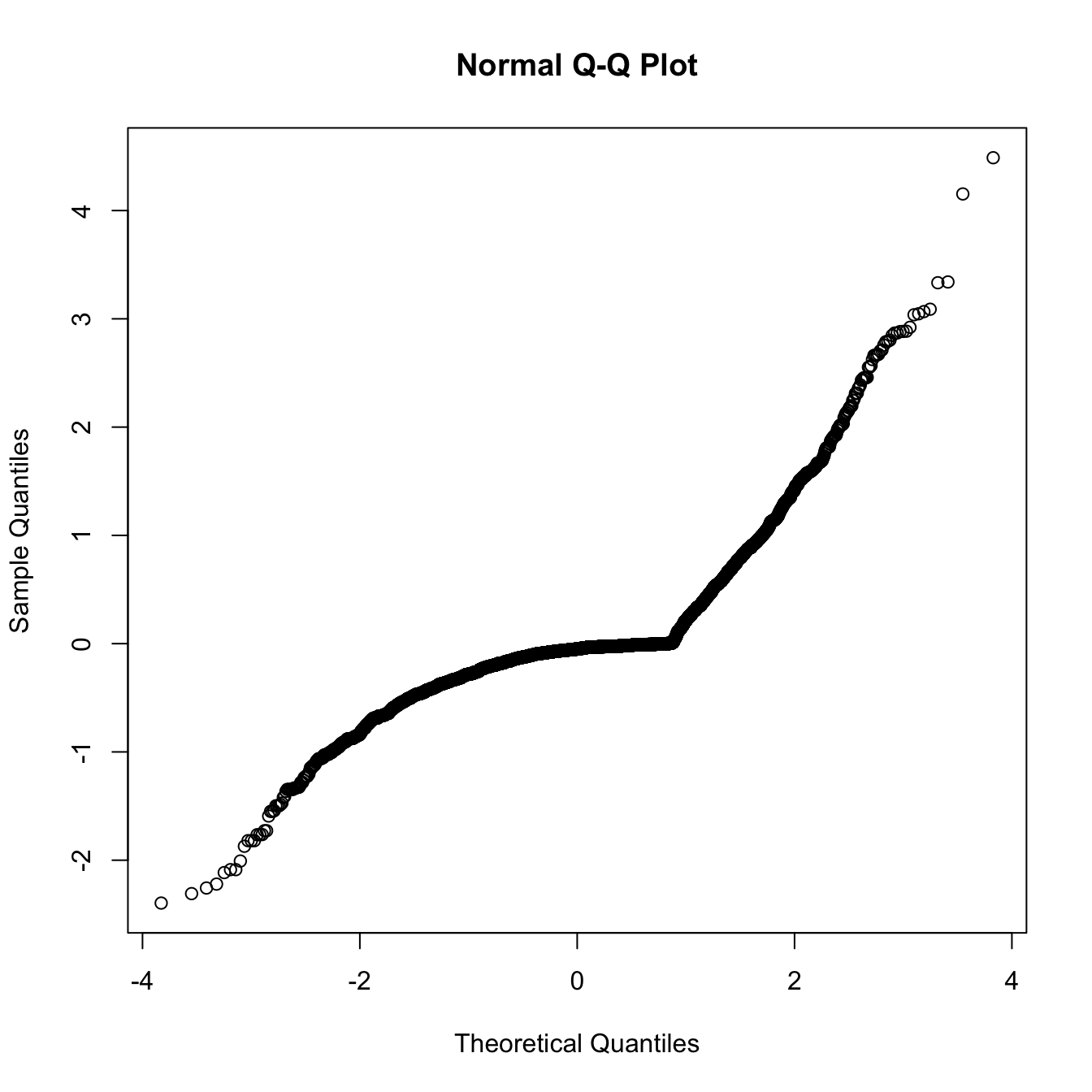
## Warning: 'sjp.lmer' is deprecated.
## Use 'plot_model' instead.
## See help("Deprecated")
Adjusting for self esteem
broad_models[[outcome]] %>%
  adjust_for_self_esteem(diary2)
##
##
## ```
## Linear mixed model fit by REML. t-tests use Satterthwaite's method ['lmerModLmerTest']
## Formula: form
## Data: diary
##
## REML criterion at convergence: 12525
##
## Scaled residuals:
## Min 1Q Median 3Q Max
## -4.804 -0.345 -0.099 -0.006 8.911
##
## Random effects:
## Groups Name Variance Std.Dev.
## person (Intercept) 0.215 0.464
## Residual 0.249 0.499
## Number of obs: 7740, groups: person, 493
##
## Fixed effects:
## Estimate Std. Error df t value Pr(>|t|)
## (Intercept) 1.28321 0.05081 1100.35046 25.25 <2e-16 ***
## includedhorm_contra -0.09248 0.05021 572.09381 -1.84 0.0660 .
## fertile 0.13236 0.05605 7321.66056 2.36 0.0182 *
## self_esteem_1 0.01928 0.00653 7726.06188 2.95 0.0032 **
## includedhorm_contra:fertile -0.18652 0.06695 7327.30450 -2.79 0.0054 **
## ---
## Signif. codes: 0 '***' 0.001 '**' 0.01 '*' 0.05 '.' 0.1 ' ' 1
##
## Correlation of Fixed Effects:
## (Intr) incld_ fertil slf__1
## inclddhrm_c -0.710
## fertile -0.226 0.234
## self_estm_1 -0.552 0.011 -0.010
## inclddhrm_: 0.195 -0.281 -0.837 -0.002
##
## ```
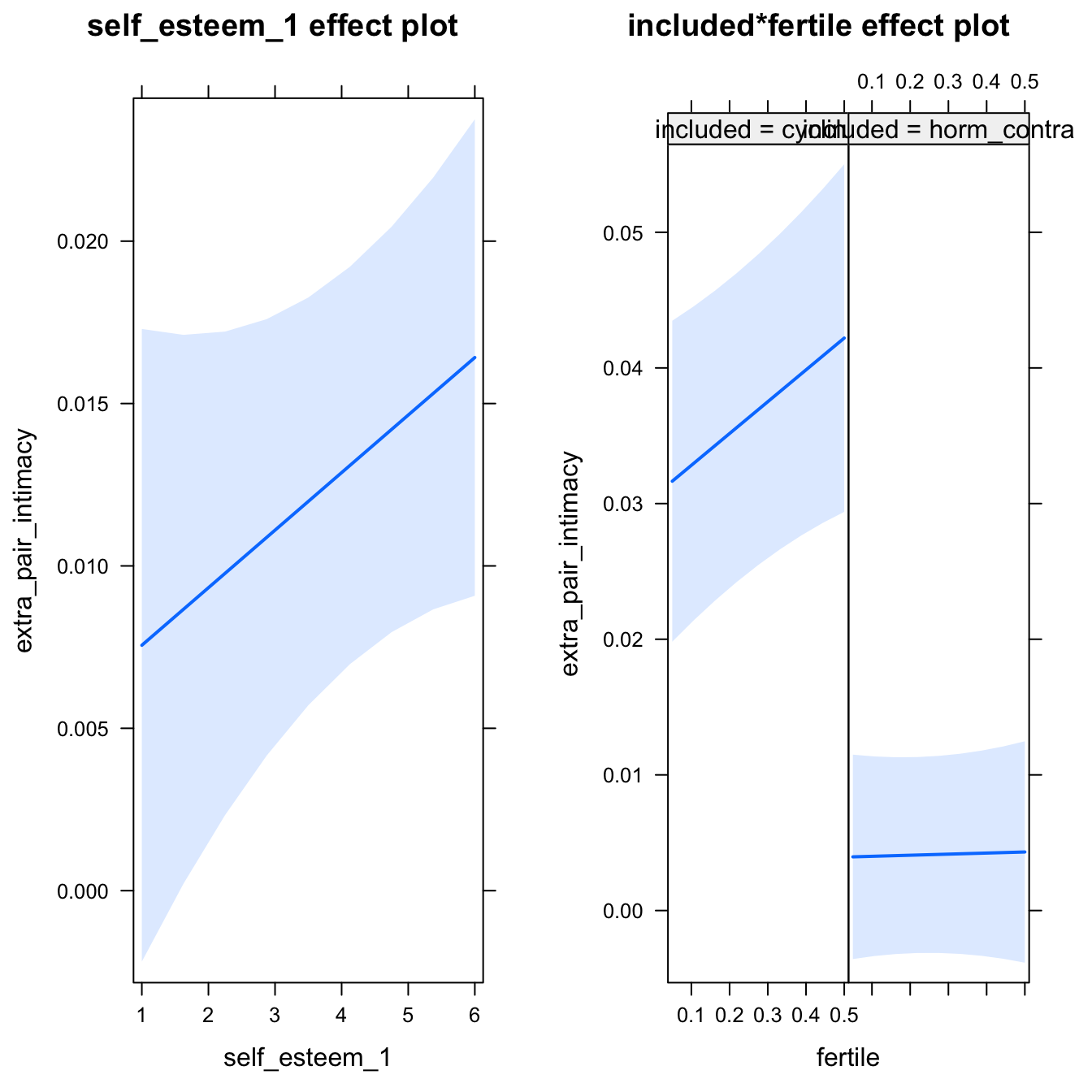
bla = 2H1.1. Extra-pair intimacy
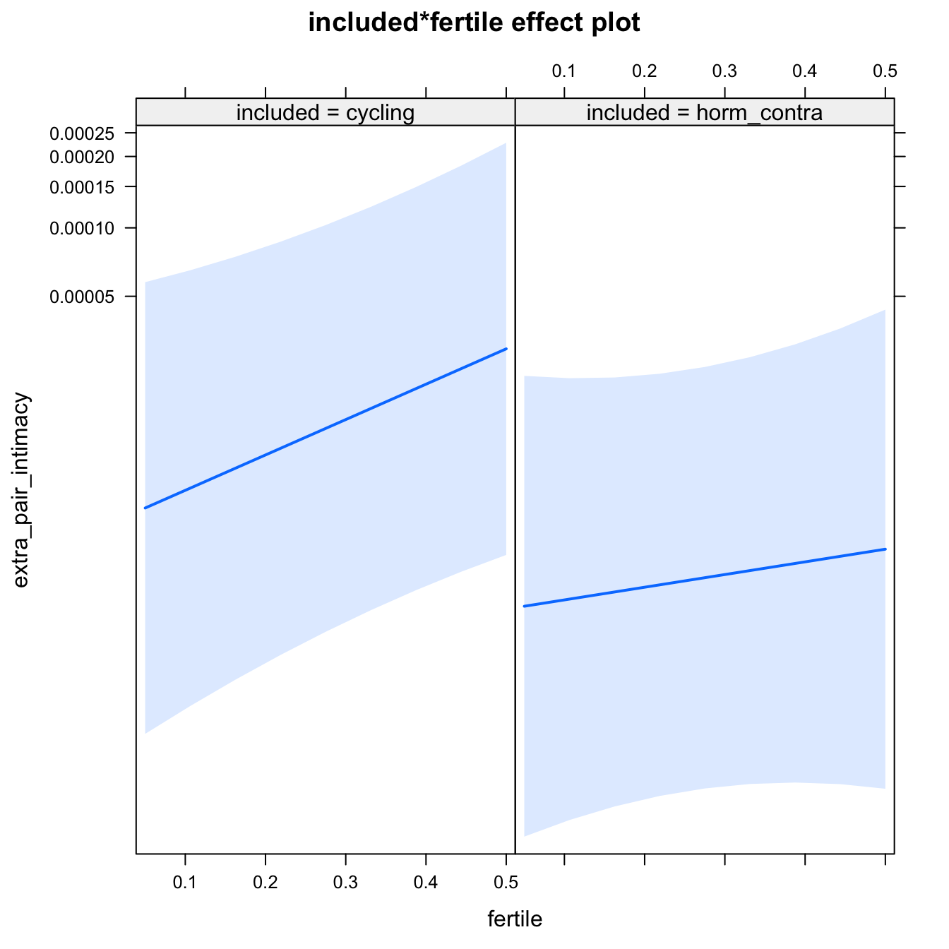
models$extra_pair_intimacy = glmer(extra_pair_intimacy ~ included * fertile + ( 1 | person), data = diary, family = binomial(link = "probit"))
do_model(models$extra_pair_intimacy, diary)
## Warning: glm.fit: algorithm did not convergeNarrow window
model %>%
  print_summary() %>%
  plot_all_effects()
Generalized linear mixed model fit by maximum likelihood (Laplace Approximation) ['glmerMod']
Family: binomial ( probit )
Formula: extra_pair_intimacy ~ included * fertile + (1 | person)
Data: diary
AIC BIC logLik deviance df.resid
526.0 559.8 -258.0 516.0 6378
Scaled residuals:
Min 1Q Median 3Q Max
-1.906 -0.002 -0.002 -0.001 4.482
Random effects:
Groups Name Variance Std.Dev.
person (Intercept) 9.77 3.13
Number of obs: 6383, groups: person, 493
Fixed effects:
Estimate Std. Error z value Pr(>|z|)
(Intercept) -4.466 0.299 -14.94 <2e-16 ***
includedhorm_contra -0.218 0.368 -0.59 0.554
fertile 0.887 0.416 2.13 0.033 *
includedhorm_contra:fertile -0.569 0.723 -0.79 0.431
---
Signif. codes: 0 '***' 0.001 '**' 0.01 '*' 0.05 '.' 0.1 ' ' 1
Correlation of Fixed Effects:
(Intr) incld_ fertil
inclddhrm_c -0.590
fertile -0.508 0.379
inclddhrm_: 0.278 -0.539 -0.573
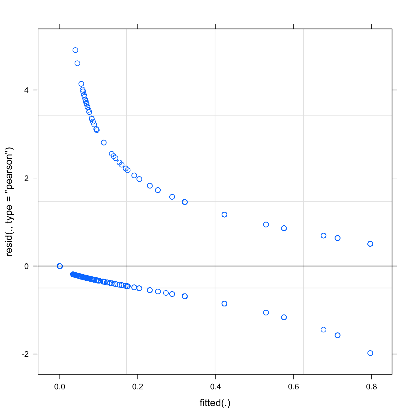
Diagnostics
model %>%
  plot_outcome(diary) %>%
  print_diagnostics()
## Error in qqnorm.default(resid(obj)): y is empty or has only NAs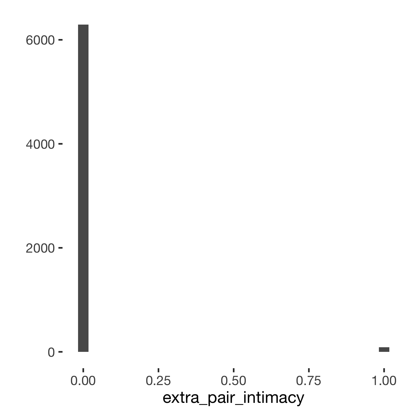
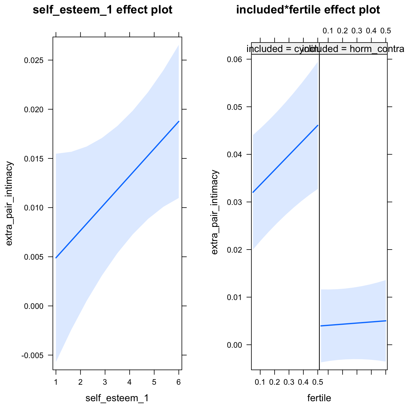
Adjusting for self esteem
model %>%
  adjust_for_self_esteem(diary)
##
##
## ```
## Linear mixed model fit by REML. t-tests use Satterthwaite's method ['lmerModLmerTest']
## Formula: form
## Data: diary
##
## REML criterion at convergence: -10945
##
## Scaled residuals:
## Min 1Q Median 3Q Max
## -7.461 -0.032 -0.012 0.006 9.968
##
## Random effects:
## Groups Name Variance Std.Dev.
## person (Intercept) 0.00424 0.0651
## Residual 0.00903 0.0950
## Number of obs: 6379, groups: person, 493
##
## Fixed effects:
## Estimate Std. Error df t value Pr(>|t|)
## (Intercept) 0.01866 0.00853 1618.32350 2.19 0.02877 *
## includedhorm_contra -0.02663 0.00745 622.71620 -3.57 0.00038 ***
## fertile 0.03123 0.01062 5998.60499 2.94 0.00328 **
## self_esteem_1 0.00277 0.00134 6264.98114 2.07 0.03879 *
## includedhorm_contra:fertile -0.02886 0.01271 6005.62284 -2.27 0.02318 *
## ---
## Signif. codes: 0 '***' 0.001 '**' 0.01 '*' 0.05 '.' 0.1 ' ' 1
##
## Correlation of Fixed Effects:
## (Intr) incld_ fertil slf__1
## inclddhrm_c -0.632
## fertile -0.232 0.268
## self_estm_1 -0.676 0.017 -0.003
## inclddhrm_: 0.199 -0.321 -0.835 -0.005
##
## ```
Broad window
outcome = names(model@frame)[1]
broad_models[[outcome]] <<- model %>%
  switch_window_to_broad(diary)
Generalized linear mixed model fit by maximum likelihood (Laplace Approximation) ['glmerMod']
Family: binomial ( probit )
Formula: extra_pair_intimacy ~ included * fertile + (1 | person)
Data: diary2
AIC BIC logLik deviance df.resid
605.7 640.4 -297.8 595.7 7740
Scaled residuals:
Min 1Q Median 3Q Max
-1.979 -0.002 -0.001 -0.001 4.907
Random effects:
Groups Name Variance Std.Dev.
person (Intercept) 9.37 3.06
Number of obs: 7745, groups: person, 493
Fixed effects:
Estimate Std. Error z value Pr(>|z|)
(Intercept) -4.439 0.284 -15.65 <2e-16 ***
includedhorm_contra -0.199 0.348 -0.57 0.57
fertile 0.695 0.432 1.61 0.11
includedhorm_contra:fertile -0.585 0.737 -0.79 0.43
---
Signif. codes: 0 '***' 0.001 '**' 0.01 '*' 0.05 '.' 0.1 ' ' 1
Correlation of Fixed Effects:
(Intr) incld_ fertil
inclddhrm_c -0.600
fertile -0.484 0.372
inclddhrm_: 0.280 -0.540 -0.586
## Warning: glm.fit: algorithm did not converge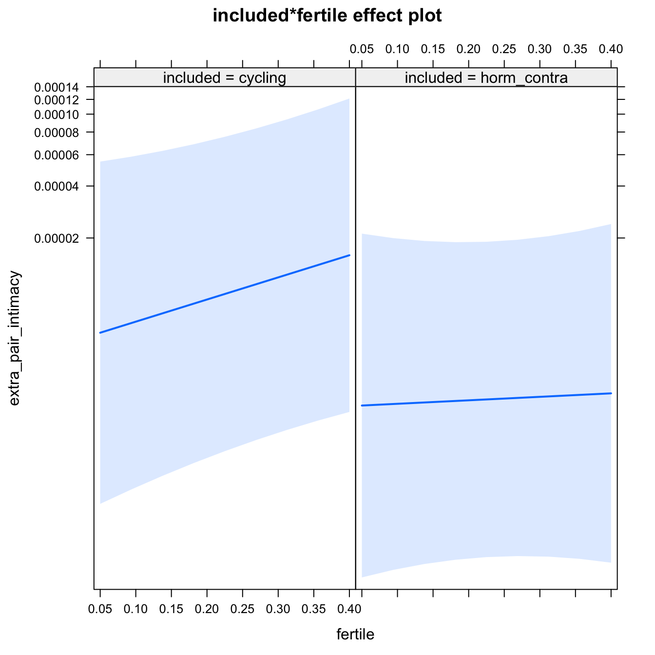
Diagnostics
## Warning: 'sjp.lmer' is deprecated.
## Use 'plot_model' instead.
## See help("Deprecated")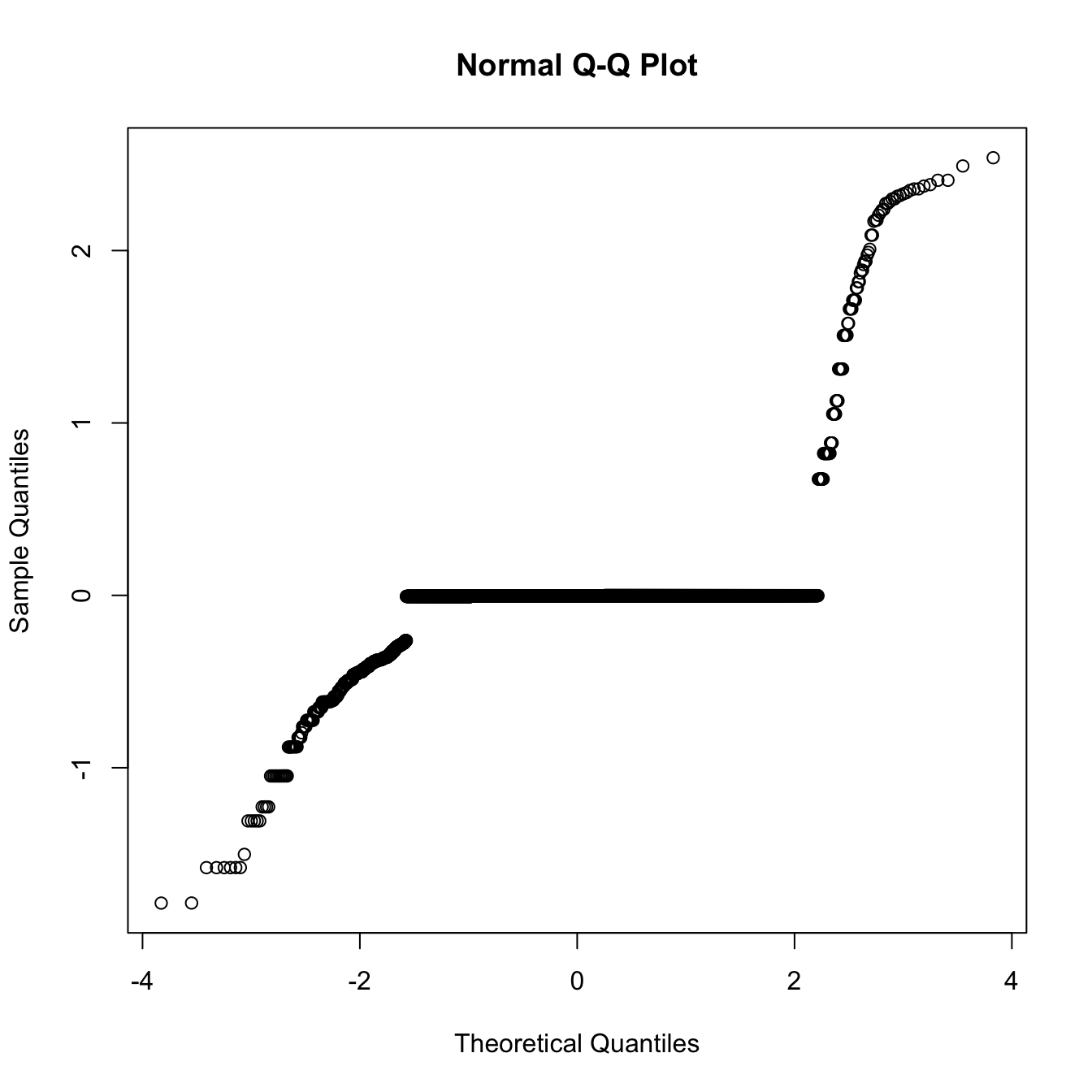
## Warning: 'sjp.lmer' is deprecated.
## Use 'plot_model' instead.
## See help("Deprecated")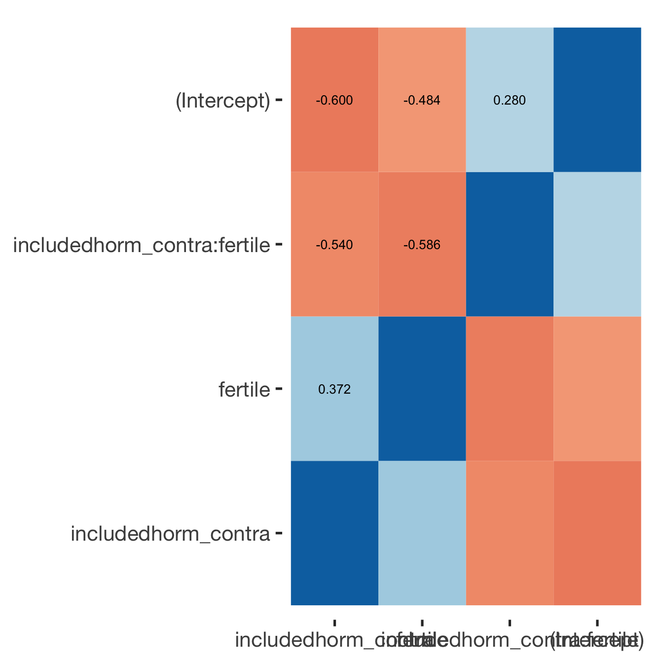
Adjusting for self esteem
broad_models[[outcome]] %>%
  adjust_for_self_esteem(diary2)
##
##
## ```
## Linear mixed model fit by REML. t-tests use Satterthwaite's method ['lmerModLmerTest']
## Formula: form
## Data: diary
##
## REML criterion at convergence: -13778
##
## Scaled residuals:
## Min 1Q Median 3Q Max
## -7.547 -0.024 -0.009 0.003 10.309
##
## Random effects:
## Groups Name Variance Std.Dev.
## person (Intercept) 0.00412 0.0642
## Residual 0.00860 0.0927
## Number of obs: 7741, groups: person, 493
##
## Fixed effects:
## Estimate Std. Error df t value Pr(>|t|)
## (Intercept) 0.02293 0.00804 1536.61550 2.85 0.00439 **
## includedhorm_contra -0.02656 0.00735 653.92543 -3.61 0.00033 ***
## fertile 0.02346 0.01039 7378.86928 2.26 0.02400 *
## self_esteem_1 0.00177 0.00119 7644.84204 1.49 0.13673
## includedhorm_contra:fertile -0.02266 0.01241 7387.39942 -1.83 0.06790 .
## ---
## Signif. codes: 0 '***' 0.001 '**' 0.01 '*' 0.05 '.' 0.1 ' ' 1
##
## Correlation of Fixed Effects:
## (Intr) incld_ fertil slf__1
## inclddhrm_c -0.659
## fertile -0.266 0.297
## self_estm_1 -0.637 0.014 -0.009
## inclddhrm_: 0.229 -0.356 -0.837 -0.002
##
## ```
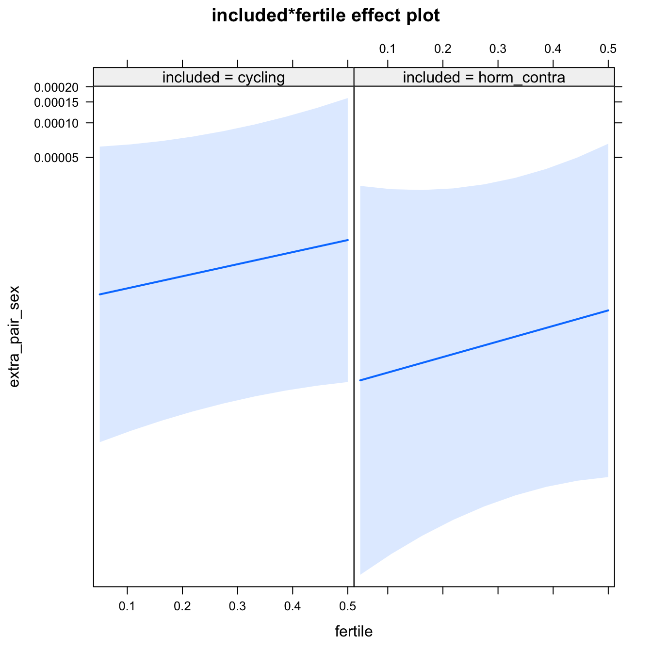
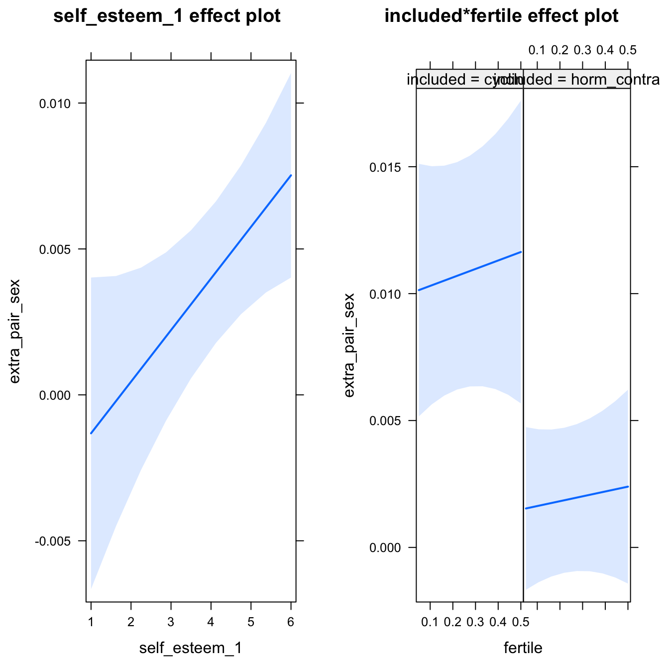
bla = 2H1.1. Extra-pair sex
models$extra_pair_sex = glmer(extra_pair_sex ~ included * fertile + ( 1 | person), data = diary, family = binomial(link = 'probit'))
do_model(models$extra_pair_sex, diary)
## Warning: glm.fit: algorithm did not convergeNarrow window
model %>%
  print_summary() %>%
  plot_all_effects()
Generalized linear mixed model fit by maximum likelihood (Laplace Approximation) ['glmerMod']
Family: binomial ( probit )
Formula: extra_pair_sex ~ included * fertile + (1 | person)
Data: diary
AIC BIC logLik deviance df.resid
254.2 288.1 -122.1 244.2 6464
Scaled residuals:
Min 1Q Median 3Q Max
-0.732 -0.002 -0.001 -0.001 4.738
Random effects:
Groups Name Variance Std.Dev.
person (Intercept) 9.81 3.13
Number of obs: 6469, groups: person, 493
Fixed effects:
Estimate Std. Error z value Pr(>|z|)
(Intercept) -4.601 0.386 -11.91 <2e-16 ***
includedhorm_contra -0.435 0.569 -0.77 0.44
fertile 0.600 0.558 1.07 0.28
includedhorm_contra:fertile 0.172 1.081 0.16 0.87
---
Signif. codes: 0 '***' 0.001 '**' 0.01 '*' 0.05 '.' 0.1 ' ' 1
Correlation of Fixed Effects:
(Intr) incld_ fertil
inclddhrm_c -0.458
fertile -0.453 0.286
inclddhrm_: 0.192 -0.622 -0.512
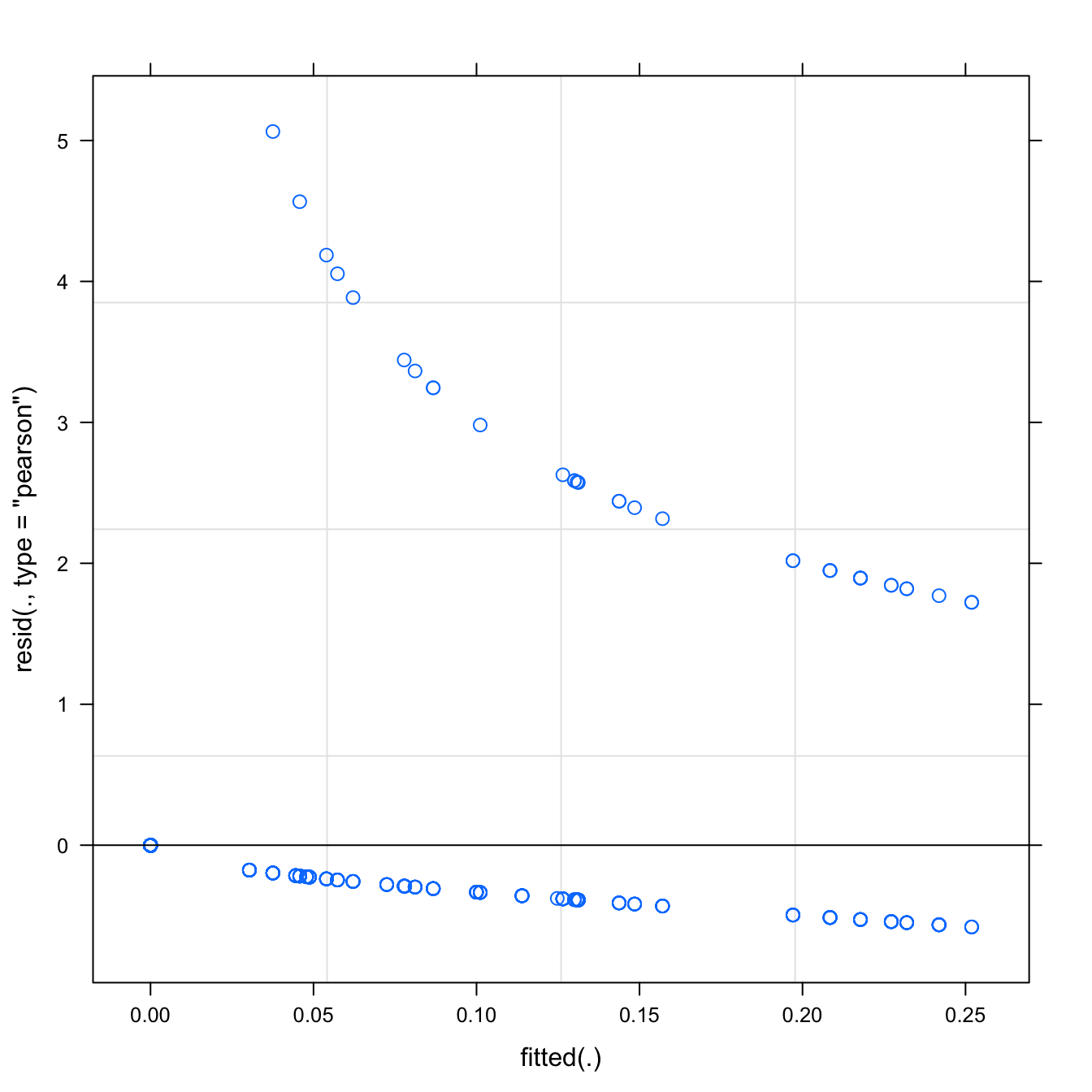
Diagnostics
model %>%
  plot_outcome(diary) %>%
  print_diagnostics()
## Error in qqnorm.default(resid(obj)): y is empty or has only NAs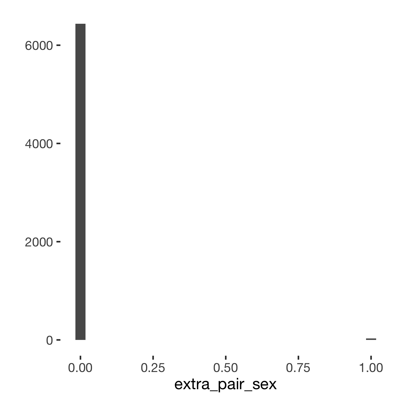
Adjusting for self esteem
model %>%
  adjust_for_self_esteem(diary)
##
##
## ```
## Linear mixed model fit by REML. t-tests use Satterthwaite's method ['lmerModLmerTest']
## Formula: form
## Data: diary
##
## REML criterion at convergence: -16226
##
## Scaled residuals:
## Min 1Q Median 3Q Max
## -3.152 -0.050 -0.025 0.001 14.727
##
## Random effects:
## Groups Name Variance Std.Dev.
## person (Intercept) 0.000517 0.0227
## Residual 0.004254 0.0652
## Number of obs: 6379, groups: person, 493
##
## Fixed effects:
## Estimate Std. Error df t value Pr(>|t|)
## (Intercept) -0.000960 0.004598 2278.584229 -0.21 0.8347
## includedhorm_contra -0.008047 0.003356 878.354801 -2.40 0.0167 *
## fertile 0.011828 0.007239 6130.846686 1.63 0.1023
## self_esteem_1 0.002444 0.000844 4494.063841 2.90 0.0038 **
## includedhorm_contra:fertile -0.009850 0.008661 6144.878744 -1.14 0.2554
## ---
## Signif. codes: 0 '***' 0.001 '**' 0.01 '*' 0.05 '.' 0.1 ' ' 1
##
## Correlation of Fixed Effects:
## (Intr) incld_ fertil slf__1
## inclddhrm_c -0.534
## fertile -0.295 0.407
## self_estm_1 -0.790 0.025 -0.003
## inclddhrm_: 0.252 -0.488 -0.836 -0.004
##
## ```
Broad window
outcome = names(model@frame)[1]
broad_models[[outcome]] <<- model %>%
  switch_window_to_broad(diary)
Generalized linear mixed model fit by maximum likelihood (Laplace Approximation) ['glmerMod']
Family: binomial ( probit )
Formula: extra_pair_sex ~ included * fertile + (1 | person)
Data: diary2
AIC BIC logLik deviance df.resid
291.2 326.1 -140.6 281.2 7846
Scaled residuals:
Min 1Q Median 3Q Max
-0.580 -0.002 -0.001 -0.001 5.064
Random effects:
Groups Name Variance Std.Dev.
person (Intercept) 9.53 3.09
Number of obs: 7851, groups: person, 493
Fixed effects:
Estimate Std. Error z value Pr(>|z|)
(Intercept) -4.536 0.364 -12.46 <2e-16 ***
includedhorm_contra -0.477 0.530 -0.90 0.37
fertile 0.206 0.594 0.35 0.73
includedhorm_contra:fertile 0.489 1.106 0.44 0.66
---
Signif. codes: 0 '***' 0.001 '**' 0.01 '*' 0.05 '.' 0.1 ' ' 1
Correlation of Fixed Effects:
(Intr) incld_ fertil
inclddhrm_c -0.476
fertile -0.404 0.270
inclddhrm_: 0.191 -0.613 -0.536
## Warning: glm.fit: algorithm did not converge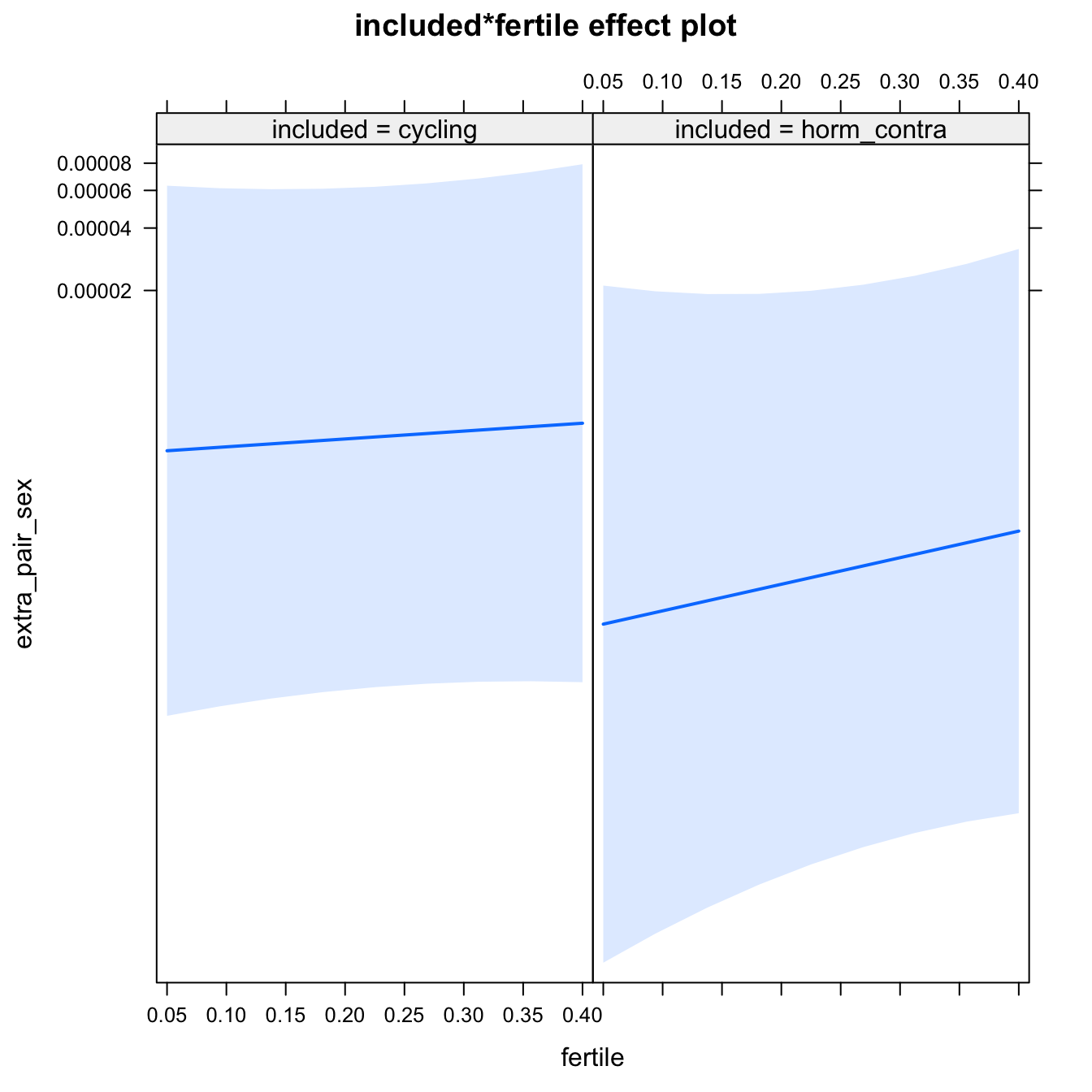
Diagnostics
## Warning: 'sjp.lmer' is deprecated.
## Use 'plot_model' instead.
## See help("Deprecated")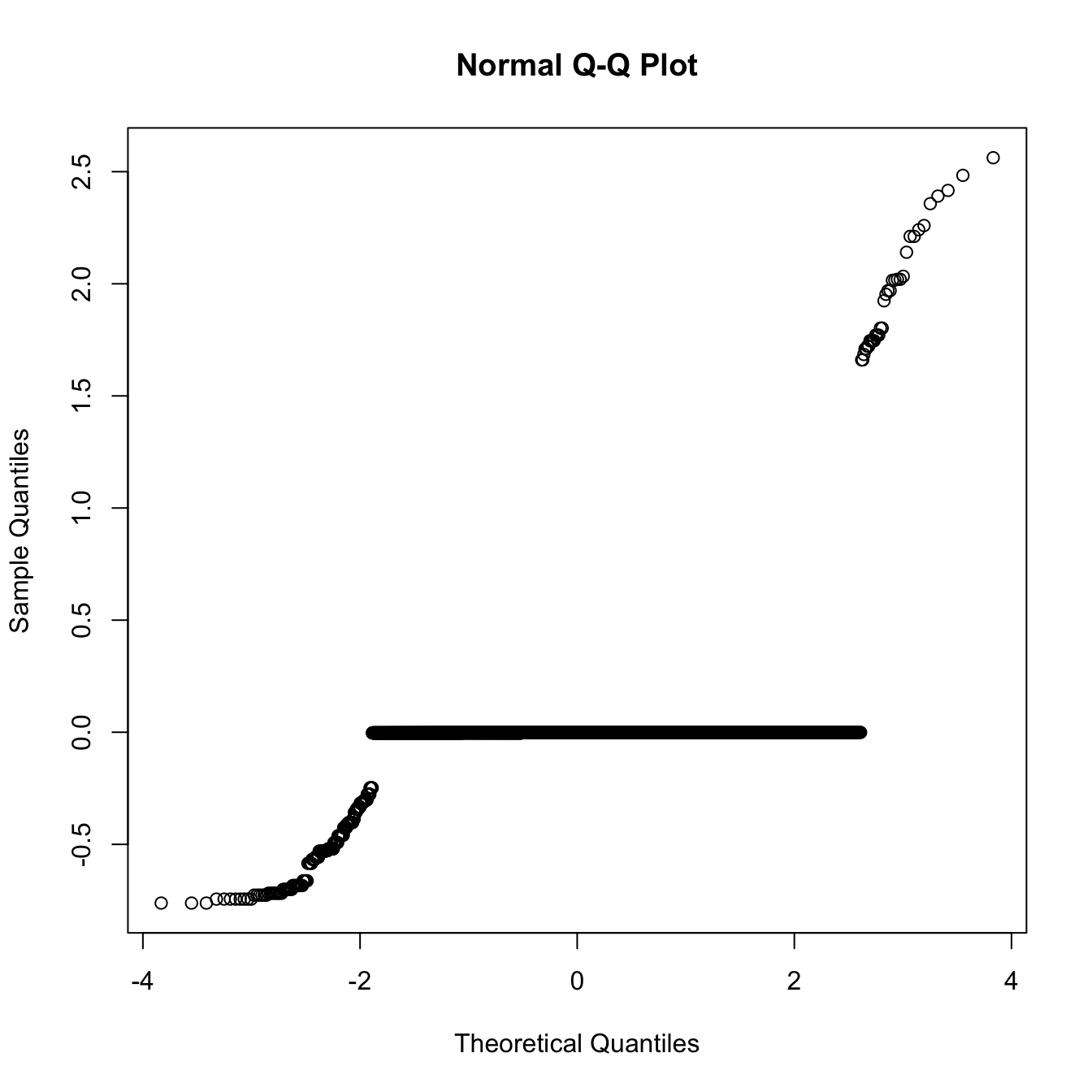
## Warning: 'sjp.lmer' is deprecated.
## Use 'plot_model' instead.
## See help("Deprecated")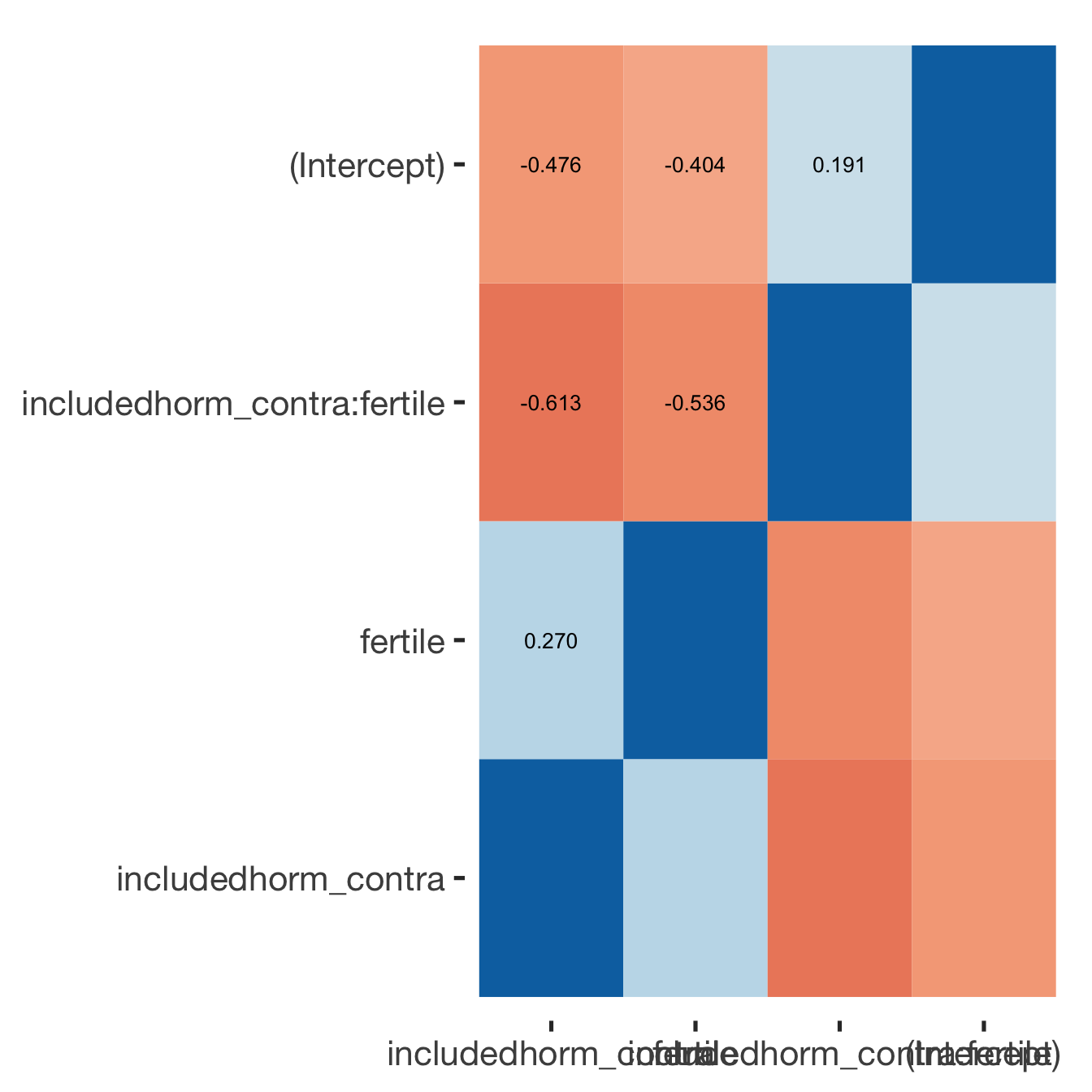
Adjusting for self esteem
broad_models[[outcome]] %>%
  adjust_for_self_esteem(diary2)
##
##
## ```
## Linear mixed model fit by REML. t-tests use Satterthwaite's method ['lmerModLmerTest']
## Formula: form
## Data: diary
##
## REML criterion at convergence: -20232
##
## Scaled residuals:
## Min 1Q Median 3Q Max
## -2.726 -0.046 -0.022 -0.003 15.268
##
## Random effects:
## Groups Name Variance Std.Dev.
## person (Intercept) 0.000457 0.0214
## Residual 0.004001 0.0633
## Number of obs: 7741, groups: person, 493
##
## Fixed effects:
## Estimate Std. Error df t value Pr(>|t|)
## (Intercept) 0.002441 0.004208 2485.287597 0.58 0.5619
## includedhorm_contra -0.008531 0.003231 1036.502977 -2.64 0.0084 **
## fertile 0.003337 0.007032 7535.421912 0.47 0.6351
## self_esteem_1 0.001768 0.000747 5308.268567 2.37 0.0180 *
## includedhorm_contra:fertile -0.001427 0.008394 7551.974784 -0.17 0.8650
## ---
## Signif. codes: 0 '***' 0.001 '**' 0.01 '*' 0.05 '.' 0.1 ' ' 1
##
## Correlation of Fixed Effects:
## (Intr) incld_ fertil slf__1
## inclddhrm_c -0.558
## fertile -0.348 0.461
## self_estm_1 -0.764 0.022 -0.008
## inclddhrm_: 0.298 -0.553 -0.838 -0.002
##
## ```
bla = 2H1.2. In-pair desire
models$in_pair_desire = lmer(in_pair_desire ~ included * fertile + ( 1 | person), data = diary)
do_model(models$in_pair_desire, diary)
Narrow window
model %>%
  print_summary() %>%
  plot_all_effects()
Linear mixed model fit by REML. t-tests use Satterthwaite's method ['lmerModLmerTest']
Formula: in_pair_desire ~ included * fertile + (1 | person)
Data: diary
REML criterion at convergence: 20169
Scaled residuals:
Min 1Q Median 3Q Max
-3.349 -0.665 -0.050 0.646 3.002
Random effects:
Groups Name Variance Std.Dev.
person (Intercept) 0.705 0.84
Residual 1.172 1.08
Number of obs: 6378, groups: person, 493
Fixed effects:
Estimate Std. Error df t value Pr(>|t|)
(Intercept) 3.4831 0.0790 576.9229 44.11 <2e-16 ***
includedhorm_contra 0.2415 0.0936 581.5434 2.58 0.0101 *
fertile 0.3122 0.1211 5969.4288 2.58 0.0100 **
includedhorm_contra:fertile -0.3874 0.1450 5975.3906 -2.67 0.0076 **
---
Signif. codes: 0 '***' 0.001 '**' 0.01 '*' 0.05 '.' 0.1 ' ' 1
Correlation of Fixed Effects:
(Intr) incld_ fertil
inclddhrm_c -0.843
fertile -0.289 0.244
inclddhrm_: 0.241 -0.292 -0.835
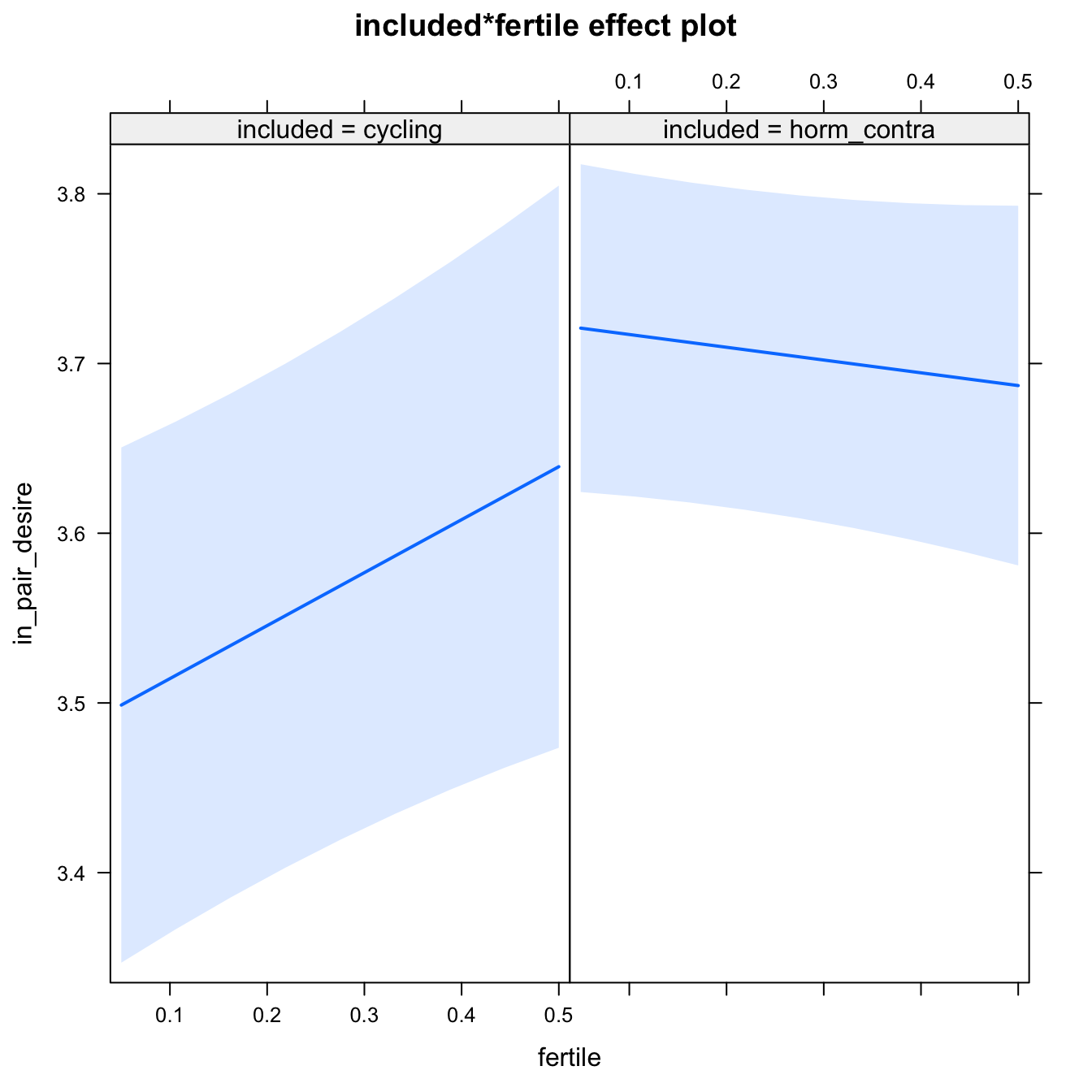
Diagnostics
model %>%
  plot_outcome(diary) %>%
  print_diagnostics()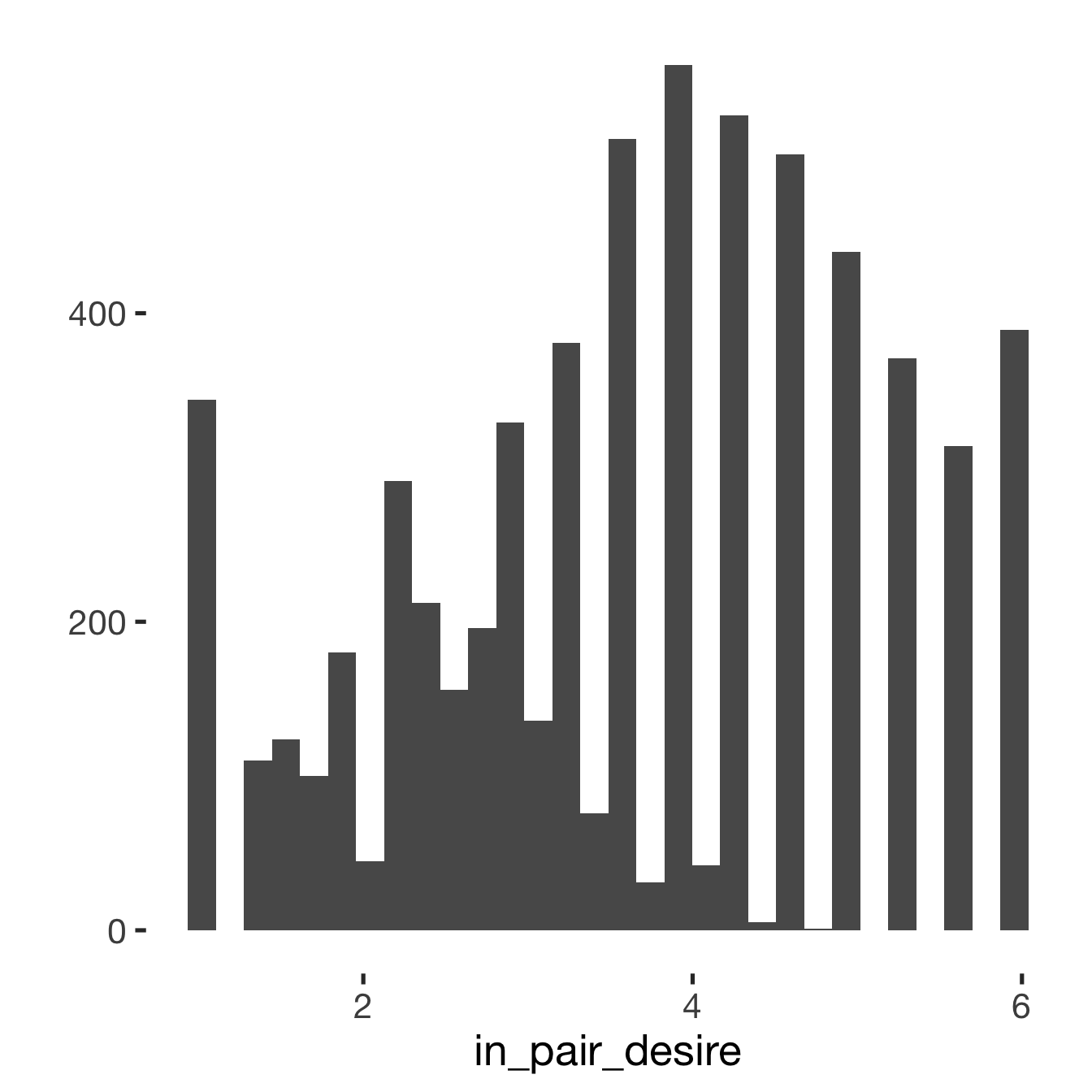
## Error in qqnorm.default(resid(obj)): y is empty or has only NAs
Adjusting for self esteem
model %>%
  adjust_for_self_esteem(diary)
##
##
## ```
## Linear mixed model fit by REML. t-tests use Satterthwaite's method ['lmerModLmerTest']
## Formula: form
## Data: diary
##
## REML criterion at convergence: 19679
##
## Scaled residuals:
## Min 1Q Median 3Q Max
## -3.340 -0.674 -0.036 0.658 3.707
##
## Random effects:
## Groups Name Variance Std.Dev.
## person (Intercept) 0.647 0.804
## Residual 1.085 1.042
## Number of obs: 6378, groups: person, 493
##
## Fixed effects:
## Estimate Std. Error df t value Pr(>|t|)
## (Intercept) 2.0305 0.0990 1414.0471 20.50 <2e-16 ***
## includedhorm_contra 0.2722 0.0897 582.1608 3.03 0.0025 **
## fertile 0.3028 0.1165 5968.9412 2.60 0.0094 **
## self_esteem_1 0.3382 0.0149 6348.1650 22.74 <2e-16 ***
## includedhorm_contra:fertile -0.4031 0.1395 5974.9404 -2.89 0.0039 **
## ---
## Signif. codes: 0 '***' 0.001 '**' 0.01 '*' 0.05 '.' 0.1 ' ' 1
##
## Correlation of Fixed Effects:
## (Intr) incld_ fertil slf__1
## inclddhrm_c -0.654
## fertile -0.219 0.244
## self_estm_1 -0.645 0.015 -0.004
## inclddhrm_: 0.188 -0.293 -0.835 -0.005
##
## ```
Broad window
outcome = names(model@frame)[1]
broad_models[[outcome]] <<- model %>%
  switch_window_to_broad(diary)
Linear mixed model fit by REML. t-tests use Satterthwaite's method ['lmerModLmerTest']
Formula: form
Data: diary2
REML criterion at convergence: 24314
Scaled residuals:
Min 1Q Median 3Q Max
-3.383 -0.667 -0.048 0.644 3.361
Random effects:
Groups Name Variance Std.Dev.
person (Intercept) 0.709 0.842
Residual 1.169 1.081
Number of obs: 7740, groups: person, 493
Fixed effects:
Estimate Std. Error df t value Pr(>|t|)
(Intercept) 3.4865 0.0793 607.0044 43.99 <2e-16 ***
includedhorm_contra 0.2410 0.0940 611.9144 2.57 0.0106 *
fertile 0.3345 0.1212 7351.7877 2.76 0.0058 **
includedhorm_contra:fertile -0.4211 0.1448 7359.3735 -2.91 0.0036 **
---
Signif. codes: 0 '***' 0.001 '**' 0.01 '*' 0.05 '.' 0.1 ' ' 1
Correlation of Fixed Effects:
(Intr) incld_ fertil
inclddhrm_c -0.843
fertile -0.321 0.271
inclddhrm_: 0.269 -0.325 -0.837
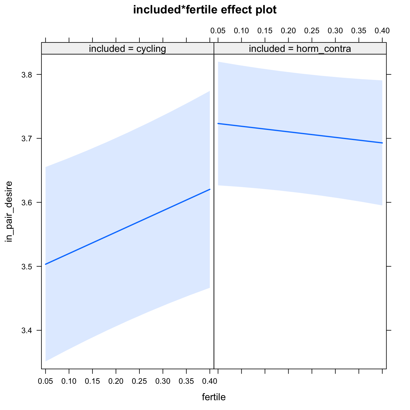
Diagnostics
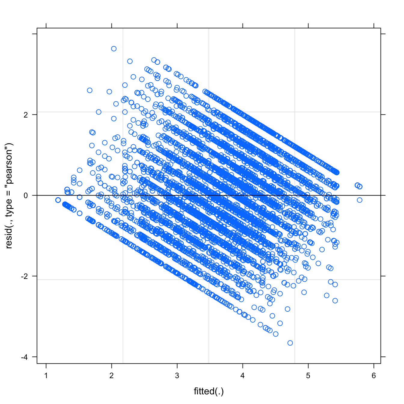
## Warning: 'sjp.lmer' is deprecated.
## Use 'plot_model' instead.
## See help("Deprecated")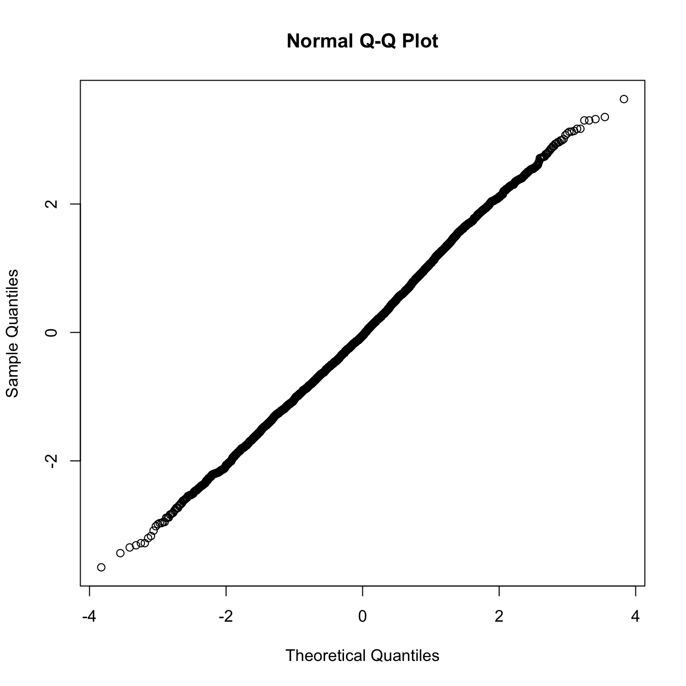
## Warning: 'sjp.lmer' is deprecated.
## Use 'plot_model' instead.
## See help("Deprecated")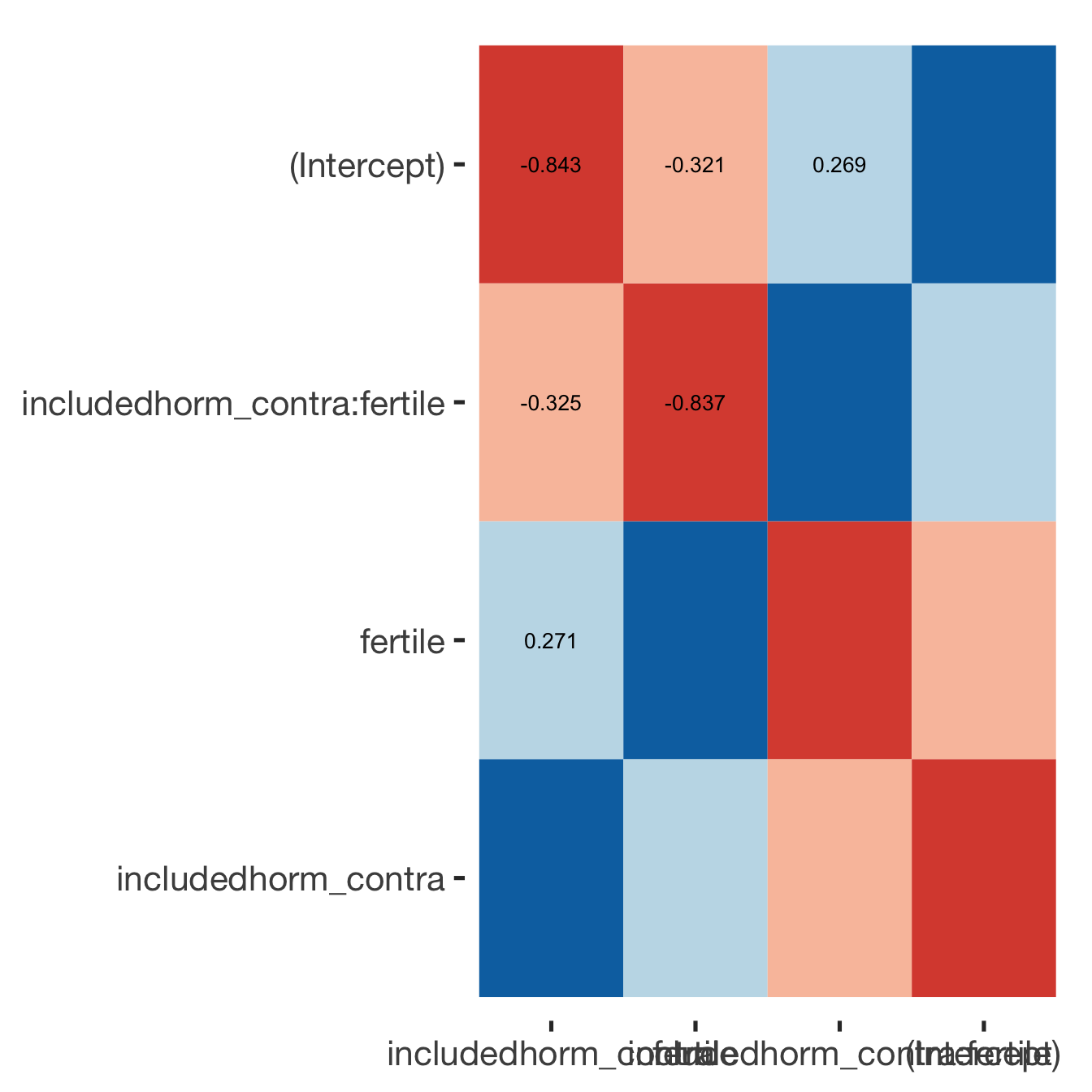
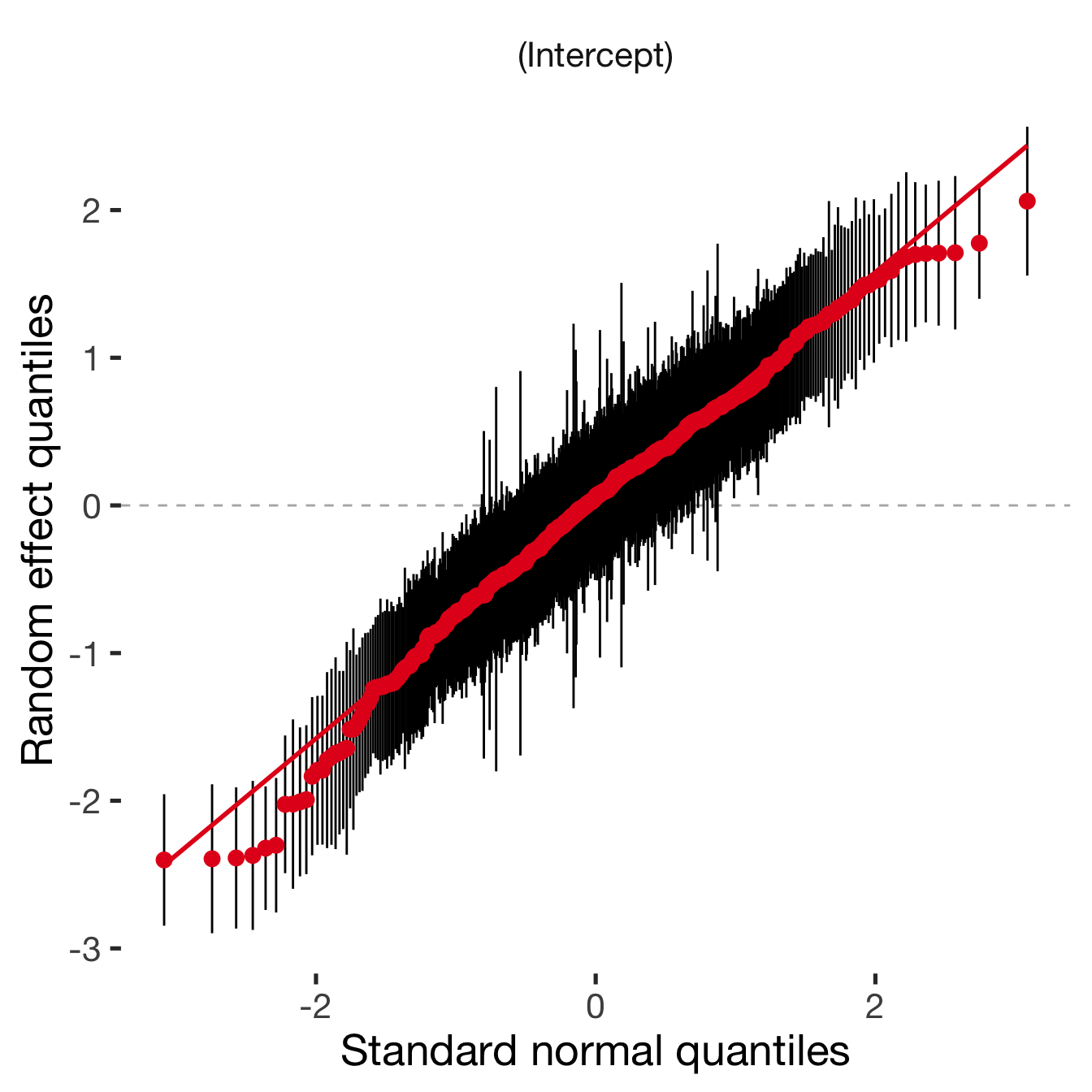
Adjusting for self esteem
broad_models[[outcome]] %>%
  adjust_for_self_esteem(diary2)
##
##
## ```
## Linear mixed model fit by REML. t-tests use Satterthwaite's method ['lmerModLmerTest']
## Formula: form
## Data: diary
##
## REML criterion at convergence: 23760
##
## Scaled residuals:
## Min 1Q Median 3Q Max
## -3.352 -0.673 -0.036 0.663 3.666
##
## Random effects:
## Groups Name Variance Std.Dev.
## person (Intercept) 0.647 0.804
## Residual 1.088 1.043
## Number of obs: 7740, groups: person, 493
##
## Fixed effects:
## Estimate Std. Error df t value Pr(>|t|)
## (Intercept) 2.0868 0.0955 1349.9129 21.85 <2e-16 ***
## includedhorm_contra 0.2697 0.0900 614.0632 3.00 0.0028 **
## fertile 0.3080 0.1170 7352.4567 2.63 0.0085 **
## self_esteem_1 0.3258 0.0135 7715.0406 24.13 <2e-16 ***
## includedhorm_contra:fertile -0.4287 0.1397 7359.9667 -3.07 0.0022 **
## ---
## Signif. codes: 0 '***' 0.001 '**' 0.01 '*' 0.05 '.' 0.1 ' ' 1
##
## Correlation of Fixed Effects:
## (Intr) incld_ fertil slf__1
## inclddhrm_c -0.678
## fertile -0.252 0.273
## self_estm_1 -0.607 0.013 -0.009
## inclddhrm_: 0.217 -0.328 -0.837 -0.002
##
## ```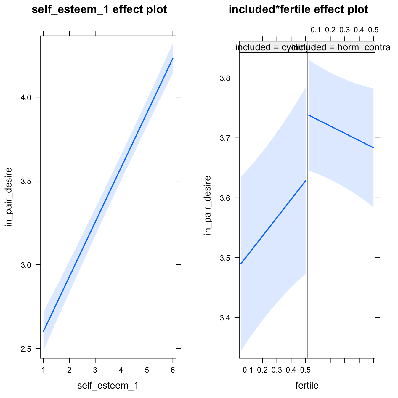
bla = 2do_moderators(models$in_pair_desire, diary)Moderators
H2_1 Partner’s physical attractiveness
Predicted fertile phase effect sizes (in red): biggest (EP desire, partner mate retention)/smallest (IP desire) when partner’s physical attractiveness is low.
model %>%
test_moderator("partner_attractiveness_physical", diary)| Df | AIC | BIC | logLik | deviance | Chisq | Chi Df | Pr(>Chisq) | |
|---|---|---|---|---|---|---|---|---|
| with_main | 8 | 20104 | 20158 | -10044 | 20088 | NA | NA | NA |
| with_mod | 10 | 20106 | 20173 | -10043 | 20086 | 2.855 | 2 | 0.2399 |
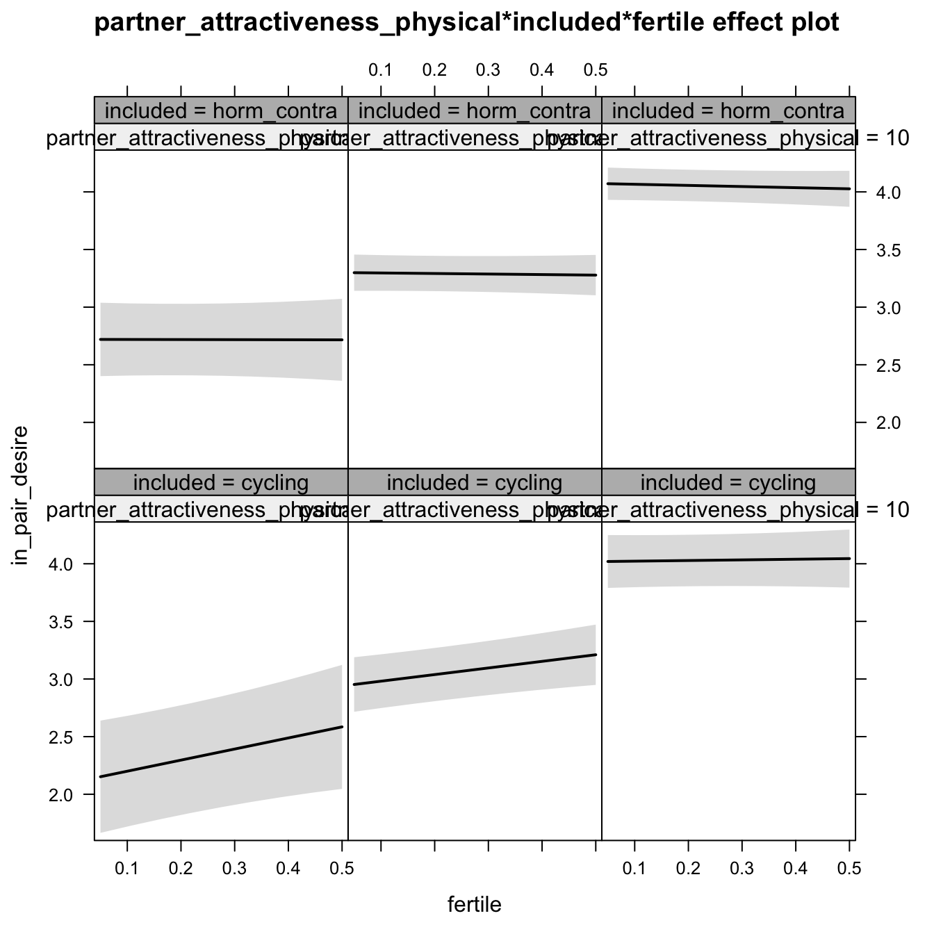
Linear mixed model fit by REML. t-tests use Satterthwaite's method ['lmerModLmerTest']
Formula: in_pair_desire ~ (1 | person) + partner_attractiveness_physical +
    included + fertile + partner_attractiveness_physical:included +
    partner_attractiveness_physical:fertile + included:fertile +
    partner_attractiveness_physical:included:fertile
   Data: diary

REML criterion at convergence: 20116

Scaled residuals:
   Min     1Q Median     3Q    Max
-3.422 -0.667 -0.042  0.657  2.987

Random effects:
 Groups   Name        Variance Std.Dev.
 person   (Intercept) 0.602    0.776
 Residual             1.172    1.083
Number of obs: 6378, groups:  person, 493

Fixed effects:
                                                             Estimate Std. Error        df t value
(Intercept)                                                    1.2839     0.3942  574.9188    3.26
partner_attractiveness_physical                                0.2733     0.0481  576.2155    5.68
includedhorm_contra                                            0.8552     0.4702  582.8906    1.82
fertile                                                        1.3498     0.6352 5961.0642    2.12
partner_attractiveness_physical:includedhorm_contra           -0.0796     0.0571  584.3870   -1.39
partner_attractiveness_physical:fertile                       -0.1294     0.0774 5964.5353   -1.67
includedhorm_contra:fertile                                   -1.3188     0.7719 5976.6192   -1.71
partner_attractiveness_physical:includedhorm_contra:fertile    0.1165     0.0937 5978.7321    1.24
                                                               Pr(>|t|)
(Intercept)                                                      0.0012 **
partner_attractiveness_physical                             0.000000021 ***
includedhorm_contra                                              0.0694 .
fertile                                                          0.0336 *
partner_attractiveness_physical:includedhorm_contra              0.1637
partner_attractiveness_physical:fertile                          0.0946 .
includedhorm_contra:fertile                                      0.0876 .
partner_attractiveness_physical:includedhorm_contra:fertile      0.2138
---
Signif. codes:  0 '***' 0.001 '**' 0.01 '*' 0.05 '.' 0.1 ' ' 1

Correlation of Fixed Effects:
            (Intr) prtn__ incld_ fertil pr__:_ prt__: incl_:
prtnr_ttrc_ -0.982
inclddhrm_c -0.838  0.823
fertile     -0.300  0.294  0.251
prtnr_tt_:_  0.827 -0.842 -0.982 -0.248
prtnr_ttr_:  0.295 -0.301 -0.247 -0.982  0.253
inclddhrm_:  0.247 -0.242 -0.305 -0.823  0.299  0.808
prtnr_t_:_: -0.244  0.249  0.300  0.811 -0.305 -0.826 -0.982
H2_1 Partner’s short-term attractiveness
Predicted fertile phase effect sizes (in red): biggest (EP desire, partner mate retention)/smallest (IP desire) when partner’s short-term attractiveness is low.
model %>%
test_moderator("partner_attractiveness_shortterm", diary)| Df | AIC | BIC | logLik | deviance | Chisq | Chi Df | Pr(>Chisq) | |
|---|---|---|---|---|---|---|---|---|
| with_main | 8 | 20108 | 20162 | -10046 | 20092 | NA | NA | NA |
| with_mod | 10 | 20106 | 20174 | -10043 | 20086 | 6.277 | 2 | 0.04335 |
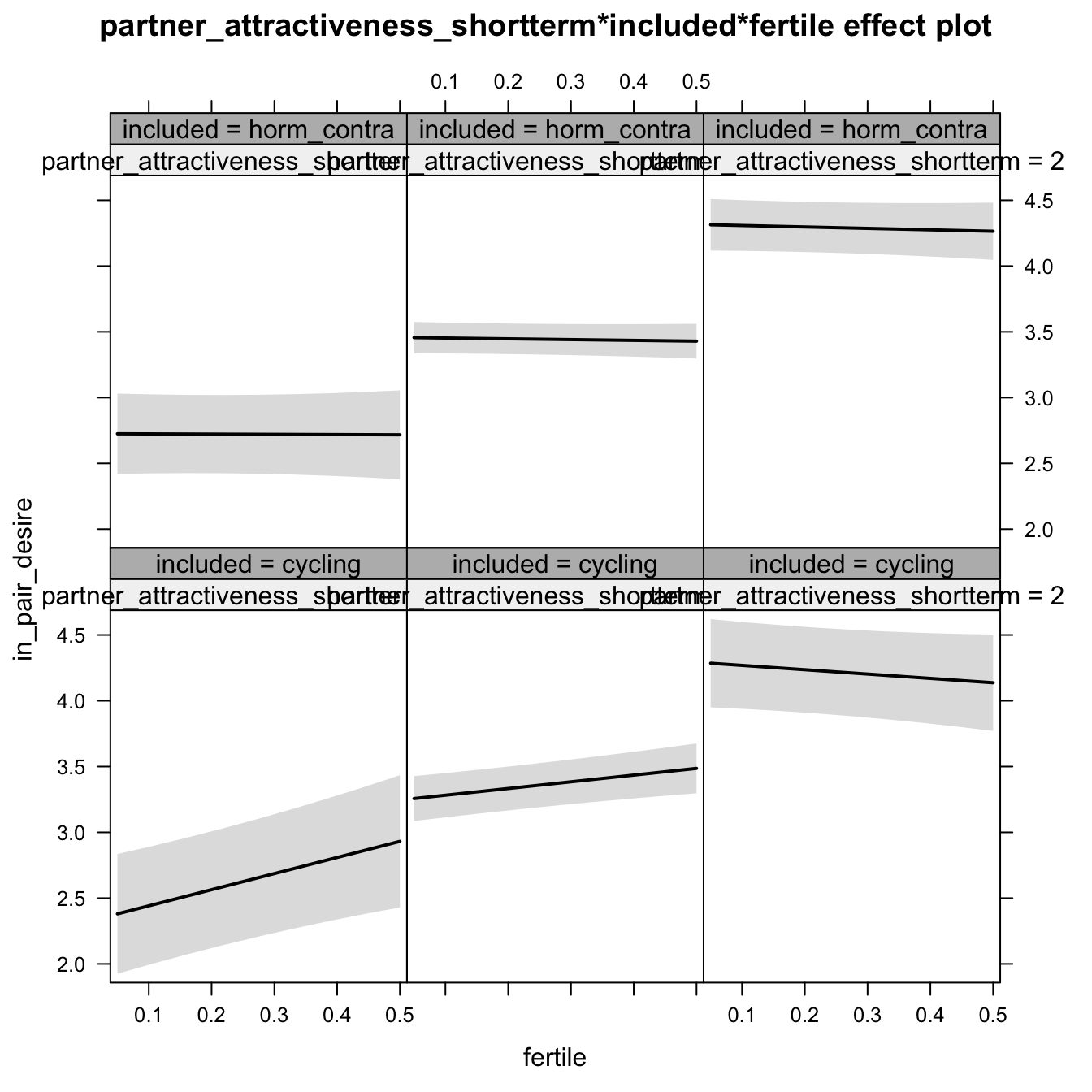
Linear mixed model fit by REML. t-tests use Satterthwaite's method ['lmerModLmerTest']
Formula: in_pair_desire ~ (1 | person) + partner_attractiveness_shortterm +
    included + fertile + partner_attractiveness_shortterm:included +
    partner_attractiveness_shortterm:fertile + included:fertile +
    partner_attractiveness_shortterm:included:fertile
   Data: diary

REML criterion at convergence: 20113

Scaled residuals:
   Min     1Q Median     3Q    Max
-3.472 -0.660 -0.044  0.660  3.005

Random effects:
 Groups   Name        Variance Std.Dev.
 person   (Intercept) 0.608    0.78
 Residual             1.172    1.08
Number of obs: 6378, groups:  person, 493

Fixed effects:
                                                              Estimate Std. Error        df t value
(Intercept)                                                     3.5088     0.0746  584.3931   47.05
partner_attractiveness_shortterm                                0.3966     0.0767  596.8022    5.17
includedhorm_contra                                             0.1731     0.0886  588.8710    1.95
fertile                                                         0.2920     0.1211 5974.5507    2.41
partner_attractiveness_shortterm:includedhorm_contra           -0.0779     0.0908  596.4784   -0.86
partner_attractiveness_shortterm:fertile                       -0.3109     0.1246 5990.9581   -2.50
includedhorm_contra:fertile                                    -0.3647     0.1452 5981.0844   -2.51
partner_attractiveness_shortterm:includedhorm_contra:fertile    0.2925     0.1486 5990.8432    1.97
                                                               Pr(>|t|)
(Intercept)                                                     < 2e-16 ***
partner_attractiveness_shortterm                             0.00000032 ***
includedhorm_contra                                               0.051 .
fertile                                                           0.016 *
partner_attractiveness_shortterm:includedhorm_contra              0.392
partner_attractiveness_shortterm:fertile                          0.013 *
includedhorm_contra:fertile                                       0.012 *
partner_attractiveness_shortterm:includedhorm_contra:fertile      0.049 *
---
Signif. codes:  0 '***' 0.001 '**' 0.01 '*' 0.05 '.' 0.1 ' ' 1

Correlation of Fixed Effects:
            (Intr) prtn__ incld_ fertil pr__:_ prt__: incl_:
prtnr_ttrc_  0.065
inclddhrm_c -0.841 -0.055
fertile     -0.307 -0.023  0.258
prtnr_tt_:_ -0.055 -0.845  0.007  0.020
prtnr_ttr_: -0.023 -0.311  0.020  0.043  0.263
inclddhrm_:  0.256  0.019 -0.310 -0.834 -0.006 -0.036
prtnr_t_:_:  0.020  0.261 -0.006 -0.036 -0.312 -0.839 -0.004
H2_1 Partner’s short-term vs long-term attractiveness
Predicted fertile phase effect sizes (in red): biggest (EP desire, partner mate retention)/smallest (IP desire) top-right (high LT, low ST), then top-left (low LT, low ST), then bottom-left (low LT, high ST), then bottom-right (high LT/ST).
add_main = update.formula(formula(model), new = as.formula(paste0(". ~ . + partner_attractiveness_longterm * included + partner_attractiveness_shortterm * included + partner_attractiveness_longterm * partner_attractiveness_shortterm"))) # reorder so that the triptych looks nice
add_mod_formula = update.formula(update.formula(formula(model), new = . ~ . - included * fertile), new = as.formula(paste0(". ~ . + partner_attractiveness_longterm * fertile * partner_attractiveness_shortterm * included"))) # reorder so that the triptych looks nice

update(model, formula = add_main) -> with_main
update(model, formula = add_mod_formula) -> with_mod
if (is(with_mod, "lmerMod")) {
  with_mod <- as_lmerModLmerTest(with_mod)
}
cat(pander(anova(with_main, with_mod)))| Df | AIC | BIC | logLik | deviance | Chisq | Chi Df | Pr(>Chisq) | |
|---|---|---|---|---|---|---|---|---|
| with_main | 11 | 20103 | 20177 | -10040 | 20081 | NA | NA | NA |
| with_mod | 18 | 20099 | 20220 | -10031 | 20063 | 18.39 | 7 | 0.01032 |
effs = allEffects(with_mod)
effs = data.frame(effs$`partner_attractiveness_longterm:fertile:partner_attractiveness_shortterm:included`) %>%
  filter(round(partner_attractiveness_longterm,1) %in% c(-3,-2,0.8),round(partner_attractiveness_shortterm,1) %in% c(-2,0.5, 2))
ggplot(effs, aes(fertile, fit, ymin = lower, ymax = upper, color = included)) +
  facet_grid(partner_attractiveness_shortterm ~ partner_attractiveness_longterm) +
  geom_smooth(stat='identity') +
  scale_color_manual(values = c("cycling" = 'red', 'horm_contra' = 'black'), guide = F) +
  scale_fill_manual(values = c("cycling" = 'red', 'horm_contra' = 'black'), guide = F) +
  ggtitle("Moderation", "top-to-bottom: short-term,\nleft-to-right: long-term attractiveness of the partner")+
  ylab(names(model@frame)[1])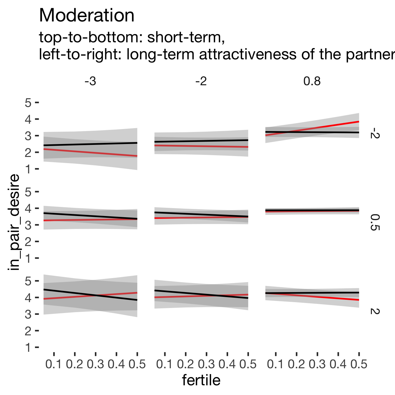
print_summary(with_mod)Linear mixed model fit by REML. t-tests use Satterthwaite's method ['lmerModLmerTest']
Formula: in_pair_desire ~ (1 | person) + partner_attractiveness_longterm +
fertile + partner_attractiveness_shortterm + included + partner_attractiveness_longterm:fertile +
partner_attractiveness_longterm:partner_attractiveness_shortterm +
fertile:partner_attractiveness_shortterm + partner_attractiveness_longterm:included +
fertile:included + partner_attractiveness_shortterm:included +
partner_attractiveness_longterm:fertile:partner_attractiveness_shortterm +
partner_attractiveness_longterm:fertile:included + partner_attractiveness_longterm:partner_attractiveness_shortterm:included +
fertile:partner_attractiveness_shortterm:included + partner_attractiveness_longterm:fertile:partner_attractiveness_shortterm:included
Data: diary
REML criterion at convergence: 20114
Scaled residuals:
Min 1Q Median 3Q Max
-3.534 -0.659 -0.042 0.654 2.978
Random effects:
Groups Name Variance Std.Dev.
person (Intercept) 0.60 0.775
Residual 1.17 1.082
Number of obs: 6378, groups: person, 493
Fixed effects:
Estimate
(Intercept) 3.50231
partner_attractiveness_longterm 0.14851
fertile 0.35138
partner_attractiveness_shortterm 0.35935
includedhorm_contra 0.18486
partner_attractiveness_longterm:fertile 0.13506
partner_attractiveness_longterm:partner_attractiveness_shortterm -0.01677
fertile:partner_attractiveness_shortterm -0.45256
partner_attractiveness_longterm:includedhorm_contra -0.07787
fertile:includedhorm_contra -0.46501
partner_attractiveness_shortterm:includedhorm_contra -0.04285
partner_attractiveness_longterm:fertile:partner_attractiveness_shortterm -0.29561
partner_attractiveness_longterm:fertile:includedhorm_contra 0.00665
partner_attractiveness_longterm:partner_attractiveness_shortterm:includedhorm_contra -0.05664
fertile:partner_attractiveness_shortterm:includedhorm_contra 0.38978
partner_attractiveness_longterm:fertile:partner_attractiveness_shortterm:includedhorm_contra 0.41820
Std. Error
(Intercept) 0.07539
partner_attractiveness_longterm 0.07845
fertile 0.12305
partner_attractiveness_shortterm 0.08191
includedhorm_contra 0.09014
partner_attractiveness_longterm:fertile 0.12786
partner_attractiveness_longterm:partner_attractiveness_shortterm 0.06306
fertile:partner_attractiveness_shortterm 0.13367
partner_attractiveness_longterm:includedhorm_contra 0.09847
fertile:includedhorm_contra 0.14900
partner_attractiveness_shortterm:includedhorm_contra 0.09616
partner_attractiveness_longterm:fertile:partner_attractiveness_shortterm 0.10536
partner_attractiveness_longterm:fertile:includedhorm_contra 0.16622
partner_attractiveness_longterm:partner_attractiveness_shortterm:includedhorm_contra 0.08865
fertile:partner_attractiveness_shortterm:includedhorm_contra 0.15851
partner_attractiveness_longterm:fertile:partner_attractiveness_shortterm:includedhorm_contra 0.15108
df
(Intercept) 577.36693
partner_attractiveness_longterm 561.37068
fertile 5968.69302
partner_attractiveness_shortterm 598.27141
includedhorm_contra 583.56402
partner_attractiveness_longterm:fertile 5949.18668
partner_attractiveness_longterm:partner_attractiveness_shortterm 569.89748
fertile:partner_attractiveness_shortterm 6001.95282
partner_attractiveness_longterm:includedhorm_contra 576.14643
fertile:includedhorm_contra 5982.21598
partner_attractiveness_shortterm:includedhorm_contra 597.88553
partner_attractiveness_longterm:fertile:partner_attractiveness_shortterm 5969.26476
partner_attractiveness_longterm:fertile:includedhorm_contra 5992.57405
partner_attractiveness_longterm:partner_attractiveness_shortterm:includedhorm_contra 580.11543
fertile:partner_attractiveness_shortterm:includedhorm_contra 6004.70675
partner_attractiveness_longterm:fertile:partner_attractiveness_shortterm:includedhorm_contra 6001.72294
t value Pr(>|t|)
(Intercept) 46.45 < 2e-16
partner_attractiveness_longterm 1.89 0.05888
fertile 2.86 0.00431
partner_attractiveness_shortterm 4.39 0.000014
includedhorm_contra 2.05 0.04073
partner_attractiveness_longterm:fertile 1.06 0.29086
partner_attractiveness_longterm:partner_attractiveness_shortterm -0.27 0.79034
fertile:partner_attractiveness_shortterm -3.39 0.00071
partner_attractiveness_longterm:includedhorm_contra -0.79 0.42936
fertile:includedhorm_contra -3.12 0.00181
partner_attractiveness_shortterm:includedhorm_contra -0.45 0.65603
partner_attractiveness_longterm:fertile:partner_attractiveness_shortterm -2.81 0.00504
partner_attractiveness_longterm:fertile:includedhorm_contra 0.04 0.96810
partner_attractiveness_longterm:partner_attractiveness_shortterm:includedhorm_contra -0.64 0.52312
fertile:partner_attractiveness_shortterm:includedhorm_contra 2.46 0.01396
partner_attractiveness_longterm:fertile:partner_attractiveness_shortterm:includedhorm_contra 2.77 0.00565
(Intercept) ***
partner_attractiveness_longterm .
fertile **
partner_attractiveness_shortterm ***
includedhorm_contra *
partner_attractiveness_longterm:fertile
partner_attractiveness_longterm:partner_attractiveness_shortterm
fertile:partner_attractiveness_shortterm ***
partner_attractiveness_longterm:includedhorm_contra
fertile:includedhorm_contra **
partner_attractiveness_shortterm:includedhorm_contra
partner_attractiveness_longterm:fertile:partner_attractiveness_shortterm **
partner_attractiveness_longterm:fertile:includedhorm_contra
partner_attractiveness_longterm:partner_attractiveness_shortterm:includedhorm_contra
fertile:partner_attractiveness_shortterm:includedhorm_contra *
partner_attractiveness_longterm:fertile:partner_attractiveness_shortterm:includedhorm_contra **
---
Signif. codes: 0 '***' 0.001 '**' 0.01 '*' 0.05 '.' 0.1 ' ' 1
H2_1b Partner’s short-term and long-term attractiveness
Edit: Alternative model specification, added after publication. Predicted fertile phase effect sizes (in red): biggest (EP desire, partner mate retention)/smallest (IP desire) top-right (high LT, low ST), then top-left (low LT, low ST), then bottom-left (low LT, high ST), then bottom-right (high LT/ST).
add_main = update.formula(formula(model), new = as.formula(paste0(". ~ . + partner_attractiveness_shortterm * included + partner_attractiveness_longterm * fertile * included"))) # reorder so that the triptych looks nice
add_mod_formula = update.formula(update.formula(formula(model), new = . ~ . - included * fertile), new = as.formula(paste0(". ~ . + (partner_attractiveness_shortterm + partner_attractiveness_longterm) * fertile * included"))) # reorder so that the triptych looks nice

update(model, formula = add_main) -> with_main
update(model, formula = add_mod_formula) -> with_mod
if (is(with_mod, "lmerMod")) {
  with_mod <- as_lmerModLmerTest(with_mod)
}
cat(pander(anova(with_main, with_mod)))| Df | AIC | BIC | logLik | deviance | Chisq | Chi Df | Pr(>Chisq) | |
|---|---|---|---|---|---|---|---|---|
| with_main | 12 | 20105 | 20187 | -10041 | 20081 | NA | NA | NA |
| with_mod | 14 | 20102 | 20196 | -10037 | 20074 | 7.661 | 2 | 0.02169 |
plot_triptych(with_mod)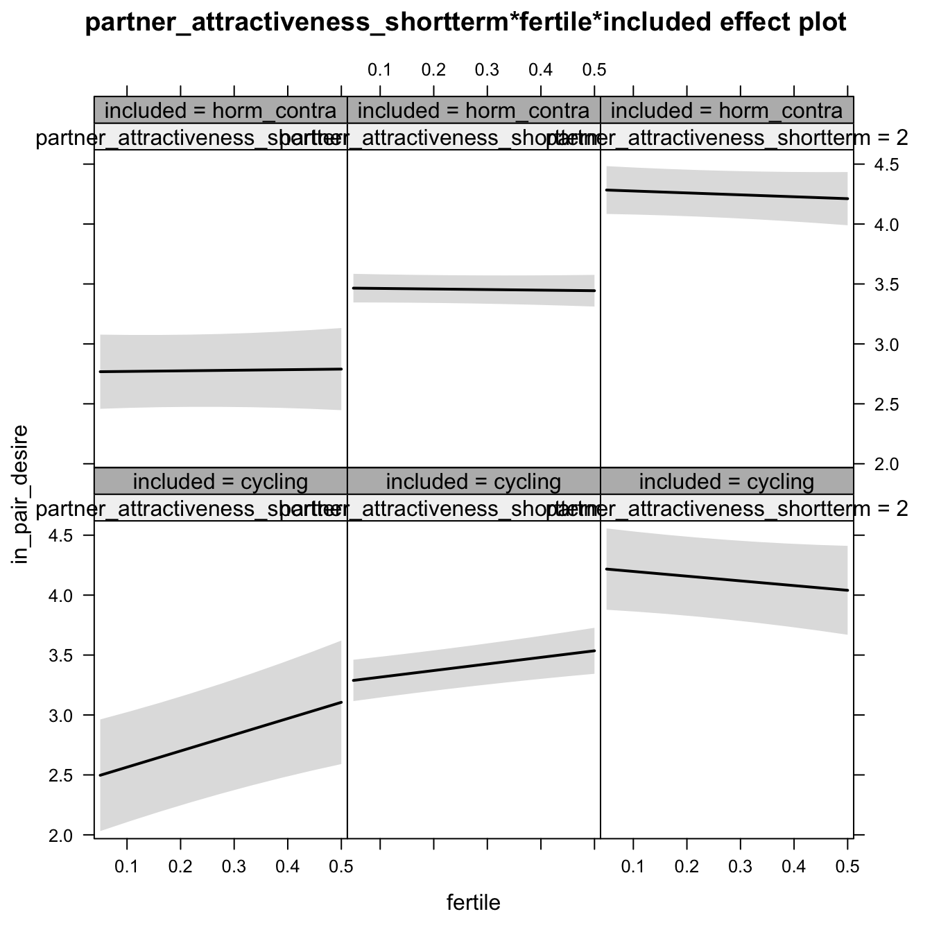
print_summary(with_mod)Linear mixed model fit by REML. t-tests use Satterthwaite's method ['lmerModLmerTest']
Formula: in_pair_desire ~ (1 | person) + partner_attractiveness_shortterm +
partner_attractiveness_longterm + fertile + included + partner_attractiveness_shortterm:fertile +
partner_attractiveness_longterm:fertile + partner_attractiveness_shortterm:included +
partner_attractiveness_longterm:included + fertile:included +
partner_attractiveness_shortterm:fertile:included + partner_attractiveness_longterm:fertile:included
Data: diary
REML criterion at convergence: 20113
Scaled residuals:
Min 1Q Median 3Q Max
-3.469 -0.660 -0.043 0.659 2.958
Random effects:
Groups Name Variance Std.Dev.
person (Intercept) 0.599 0.774
Residual 1.171 1.082
Number of obs: 6378, groups: person, 493
Fixed effects:
Estimate Std. Error df t value Pr(>|t|)
(Intercept) 3.4988 0.0743 582.4360 47.10 < 2e-16
partner_attractiveness_shortterm 0.3615 0.0785 594.0064 4.61 0.000005
partner_attractiveness_longterm 0.1522 0.0779 565.6754 1.95 0.0512
fertile 0.2886 0.1211 5972.4518 2.38 0.0172
includedhorm_contra 0.1749 0.0885 587.1784 1.98 0.0486
partner_attractiveness_shortterm:fertile -0.3492 0.1283 5988.6857 -2.72 0.0065
partner_attractiveness_longterm:fertile 0.1634 0.1275 5952.0721 1.28 0.2001
partner_attractiveness_shortterm:includedhorm_contra -0.0563 0.0928 594.8036 -0.61 0.5443
partner_attractiveness_longterm:includedhorm_contra -0.0764 0.0979 579.3557 -0.78 0.4354
fertile:includedhorm_contra -0.3778 0.1459 5981.5918 -2.59 0.0096
partner_attractiveness_shortterm:fertile:includedhorm_contra 0.3075 0.1529 5991.2891 2.01 0.0443
partner_attractiveness_longterm:fertile:includedhorm_contra -0.0372 0.1654 5990.7459 -0.22 0.8222
(Intercept) ***
partner_attractiveness_shortterm ***
partner_attractiveness_longterm .
fertile *
includedhorm_contra *
partner_attractiveness_shortterm:fertile **
partner_attractiveness_longterm:fertile
partner_attractiveness_shortterm:includedhorm_contra
partner_attractiveness_longterm:includedhorm_contra
fertile:includedhorm_contra **
partner_attractiveness_shortterm:fertile:includedhorm_contra *
partner_attractiveness_longterm:fertile:includedhorm_contra
---
Signif. codes: 0 '***' 0.001 '**' 0.01 '*' 0.05 '.' 0.1 ' ' 1
Correlation of Fixed Effects:
(Intr) prtnr_ttrctvnss_s prtnr_ttrctvnss_l fertil incld_ prtnr_ttrctvnss_s:
prtnr_ttrctvnss_s 0.076
prtnr_ttrctvnss_l -0.057 -0.232
fertile -0.308 -0.024 0.005
inclddhrm_c -0.840 -0.064 0.047 0.259
prtnr_ttrctvnss_s: -0.024 -0.313 0.073 0.047 0.020
prtnr_ttrctvnss_l: 0.005 0.072 -0.297 -0.020 -0.004 -0.238
prtnr_ttrctvnss_s:_ -0.064 -0.846 0.197 0.020 0.025 0.265
prtnr_ttrctvnss_l:_ 0.045 0.185 -0.795 -0.004 -0.083 -0.058
frtl:ncldd_ 0.256 0.020 -0.004 -0.830 -0.311 -0.039
prtnr_ttrctvnss_s::_ 0.020 0.263 -0.061 -0.039 -0.010 -0.839
prtnr_ttrctvnss_l::_ -0.004 -0.056 0.229 0.015 0.019 0.183
prtnr_ttrctvnss_l: prtnr_ttrctvnss_s:_ prtnr_ttrctvnss_l:_ frtl:_ prtnr_ttrctvnss_s::_
prtnr_ttrctvnss_s
prtnr_ttrctvnss_l
fertile
inclddhrm_c
prtnr_ttrctvnss_s:
prtnr_ttrctvnss_l:
prtnr_ttrctvnss_s:_ -0.061
prtnr_ttrctvnss_l:_ 0.237 -0.227
frtl:ncldd_ 0.016 -0.010 0.019
prtnr_ttrctvnss_s::_ 0.199 -0.314 0.074 0.011
prtnr_ttrctvnss_l::_ -0.771 0.072 -0.303 -0.071 -0.236
H2_1c Partner’s short-term minus long-term attractiveness
Edit: Alternative model specification, added after publication. Predicted fertile phase effect sizes (in red): biggest (EP desire, partner mate retention)/smallest (IP desire) top-right (high LT, low ST), then top-left (low LT, low ST), then bottom-left (low LT, high ST), then bottom-right (high LT/ST).
add_main = update.formula(formula(model), new = as.formula(paste0(". ~ . + partner_st_vs_lt * included"))) # reorder so that the triptych looks nice
add_mod_formula = update.formula(update.formula(formula(model), new = . ~ . - included * fertile), new = as.formula(paste0(". ~ . + partner_st_vs_lt * fertile * included"))) # reorder so that the triptych looks nice

update(model, formula = add_main) -> with_main
update(model, formula = add_mod_formula) -> with_mod
if (is(with_mod, "lmerMod")) {
  with_mod <- as_lmerModLmerTest(with_mod)
}
cat(pander(anova(with_main, with_mod)))| Df | AIC | BIC | logLik | deviance | Chisq | Chi Df | Pr(>Chisq) | |
|---|---|---|---|---|---|---|---|---|
| with_main | 8 | 20160 | 20214 | -10072 | 20144 | NA | NA | NA |
| with_mod | 10 | 20157 | 20224 | -10068 | 20137 | 7.188 | 2 | 0.02749 |
plot_triptych(with_mod)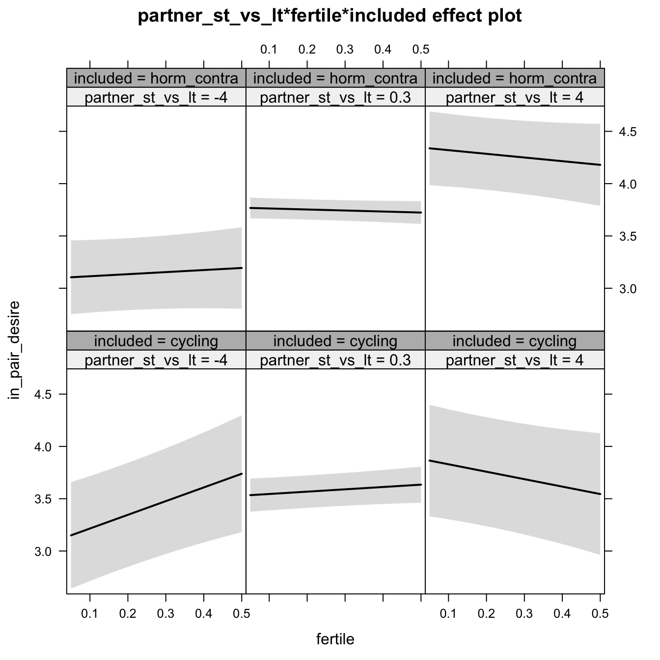
print_summary(with_mod)Linear mixed model fit by REML. t-tests use Satterthwaite's method ['lmerModLmerTest']
Formula: in_pair_desire ~ (1 | person) + partner_st_vs_lt + fertile +
included + partner_st_vs_lt:fertile + partner_st_vs_lt:included +
fertile:included + partner_st_vs_lt:fertile:included
Data: diary
REML criterion at convergence: 20164
Scaled residuals:
Min 1Q Median 3Q Max
-3.385 -0.661 -0.052 0.649 2.971
Random effects:
Groups Name Variance Std.Dev.
person (Intercept) 0.689 0.83
Residual 1.171 1.08
Number of obs: 6378, groups: person, 493
Fixed effects:
Estimate Std. Error df t value Pr(>|t|)
(Intercept) 3.4924 0.0785 574.7763 44.48 <2e-16 ***
partner_st_vs_lt 0.1020 0.0649 569.6346 1.57 0.1164
fertile 0.2987 0.1211 5966.0663 2.47 0.0137 *
includedhorm_contra 0.2327 0.0930 579.5851 2.50 0.0126 *
partner_st_vs_lt:fertile -0.2526 0.1006 5962.7507 -2.51 0.0121 *
partner_st_vs_lt:includedhorm_contra 0.0555 0.0785 576.8118 0.71 0.4797
fertile:includedhorm_contra -0.3755 0.1450 5973.0522 -2.59 0.0096 **
partner_st_vs_lt:fertile:includedhorm_contra 0.1839 0.1240 5980.8600 1.48 0.1379
---
Signif. codes: 0 '***' 0.001 '**' 0.01 '*' 0.05 '.' 0.1 ' ' 1
Correlation of Fixed Effects:
(Intr) prt___ fertil incld_ pr___: p___:_ frtl:_
prtnr_st_v_ 0.085
fertile -0.291 -0.017
inclddhrm_c -0.844 -0.072 0.246
prtnr_st__: -0.017 -0.289 0.042 0.015
prtnr_s__:_ -0.070 -0.826 0.014 0.060 0.239
frtl:ncldd_ 0.243 0.015 -0.835 -0.294 -0.035 -0.014
prtnr___::_ 0.014 0.235 -0.034 -0.014 -0.812 -0.293 0.038
H2_3 Relative attractiveness to self
Predicted fertile phase effect sizes (in red): biggest (EP desire, partner mate retention)/smallest (IP desire) when partner’s relative attractiveness is low.
model %>%
test_moderator("partner_attractiveness_rel_to_self", diary)| Df | AIC | BIC | logLik | deviance | Chisq | Chi Df | Pr(>Chisq) | |
|---|---|---|---|---|---|---|---|---|
| with_main | 8 | 20170 | 20224 | -10077 | 20154 | NA | NA | NA |
| with_mod | 10 | 20171 | 20239 | -10076 | 20151 | 3.043 | 2 | 0.2184 |
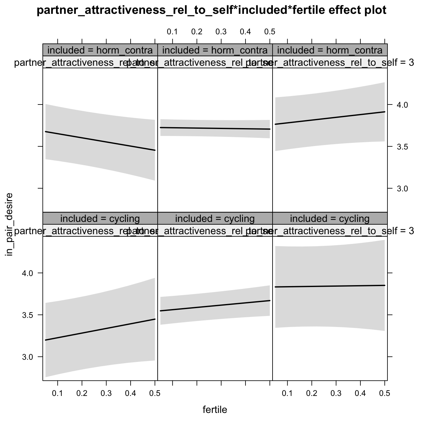
Linear mixed model fit by REML. t-tests use Satterthwaite's method ['lmerModLmerTest']
Formula: in_pair_desire ~ (1 | person) + partner_attractiveness_rel_to_self +
    included + fertile + partner_attractiveness_rel_to_self:included +
    partner_attractiveness_rel_to_self:fertile + included:fertile +
    partner_attractiveness_rel_to_self:included:fertile
   Data: diary

REML criterion at convergence: 20177

Scaled residuals:
   Min     1Q Median     3Q    Max
-3.370 -0.662 -0.050  0.656  3.012

Random effects:
 Groups   Name        Variance Std.Dev.
 person   (Intercept) 0.705    0.839
 Residual             1.172    1.083
Number of obs: 6378, groups:  person, 493

Fixed effects:
                                                                Estimate Std. Error        df t value
(Intercept)                                                       3.5009     0.0799  576.0073   43.82
partner_attractiveness_rel_to_self                                0.1100     0.0764  575.5836    1.44
includedhorm_contra                                               0.2235     0.0944  580.0977    2.37
fertile                                                           0.2973     0.1230 5969.5054    2.42
partner_attractiveness_rel_to_self:includedhorm_contra           -0.1022     0.0935  580.5818   -1.09
partner_attractiveness_rel_to_self:fertile                       -0.0856     0.1243 5998.8492   -0.69
includedhorm_contra:fertile                                      -0.3794     0.1466 5974.7449   -2.59
partner_attractiveness_rel_to_self:includedhorm_contra:fertile    0.2228     0.1509 5995.6605    1.48
                                                               Pr(>|t|)
(Intercept)                                                      <2e-16 ***
partner_attractiveness_rel_to_self                               0.1507
includedhorm_contra                                              0.0183 *
fertile                                                          0.0156 *
partner_attractiveness_rel_to_self:includedhorm_contra           0.2749
partner_attractiveness_rel_to_self:fertile                       0.4910
includedhorm_contra:fertile                                      0.0097 **
partner_attractiveness_rel_to_self:includedhorm_contra:fertile   0.1400
---
Signif. codes:  0 '***' 0.001 '**' 0.01 '*' 0.05 '.' 0.1 ' ' 1

Correlation of Fixed Effects:
            (Intr) pr____ incld_ fertil pr____:_ pr____: incl_:
prtnr_tt___  0.154
inclddhrm_c -0.846 -0.130
fertile     -0.290 -0.050  0.245
prtnr____:_ -0.126 -0.817  0.091  0.041
prtnr_t___: -0.048 -0.286  0.041  0.175  0.234
inclddhrm_:  0.243  0.042 -0.292 -0.839 -0.029   -0.146
prtn____:_:  0.039  0.236 -0.028 -0.144 -0.289   -0.823   0.104
H1.3. Sexual intercourse
models$had_sexual_intercourse = glmer(had_sexual_intercourse ~ included * fertile + ( 1 | person), data = diary, family = binomial(link = "probit"))
do_model(models$had_sexual_intercourse, diary)
Narrow window
model %>%
  print_summary() %>%
  plot_all_effects()
Generalized linear mixed model fit by maximum likelihood (Laplace Approximation) ['glmerMod']
Family: binomial ( probit )
Formula: had_sexual_intercourse ~ included * fertile + (1 | person)
Data: diary
AIC BIC logLik deviance df.resid
6469 6503 -3230 6459 6378
Scaled residuals:
Min 1Q Median 3Q Max
-1.530 -0.526 -0.400 -0.269 3.243
Random effects:
Groups Name Variance Std.Dev.
person (Intercept) 0.248 0.498
Number of obs: 6383, groups: person, 493
Fixed effects:
Estimate Std. Error z value Pr(>|z|)
(Intercept) -0.9836 0.0661 -14.89 <2e-16 ***
includedhorm_contra 0.1710 0.0770 2.22 0.026 *
fertile 0.1187 0.1692 0.70 0.483
includedhorm_contra:fertile -0.2556 0.2007 -1.27 0.203
---
Signif. codes: 0 '***' 0.001 '**' 0.01 '*' 0.05 '.' 0.1 ' ' 1
Correlation of Fixed Effects:
(Intr) incld_ fertil
inclddhrm_c -0.845
fertile -0.494 0.423
inclddhrm_: 0.418 -0.498 -0.843
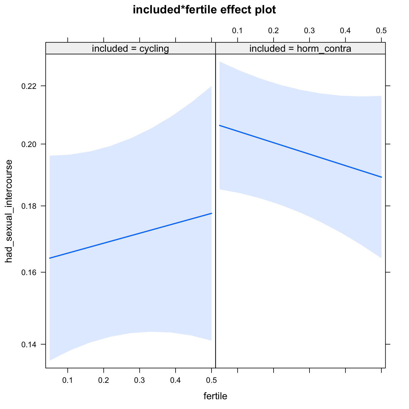
Diagnostics
model %>%
  plot_outcome(diary) %>%
  print_diagnostics()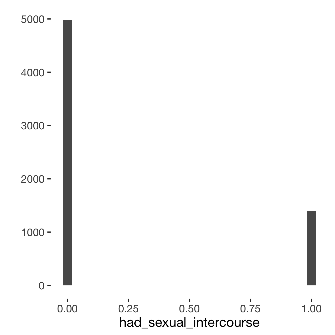
## Error in qqnorm.default(resid(obj)): y is empty or has only NAs
Adjusting for self esteem
model %>%
  adjust_for_self_esteem(diary)
##
##
## ```
## Linear mixed model fit by REML. t-tests use Satterthwaite's method ['lmerModLmerTest']
## Formula: form
## Data: diary
##
## REML criterion at convergence: 6541
##
## Scaled residuals:
## Min 1Q Median 3Q Max
## -1.744 -0.596 -0.378 -0.103 2.538
##
## Random effects:
## Groups Name Variance Std.Dev.
## person (Intercept) 0.0182 0.135
## Residual 0.1514 0.389
## Number of obs: 6379, groups: person, 493
##
## Fixed effects:
## Estimate Std. Error df t value Pr(>|t|)
## (Intercept) 0.03180 0.02740 2122.91589 1.16 0.246
## includedhorm_contra 0.04140 0.01998 801.36334 2.07 0.039 *
## fertile 0.02981 0.04318 6105.14730 0.69 0.490
## self_esteem_1 0.03842 0.00503 4330.07584 7.64 2.7e-14 ***
## includedhorm_contra:fertile -0.07300 0.05167 6120.70007 -1.41 0.158
## ---
## Signif. codes: 0 '***' 0.001 '**' 0.01 '*' 0.05 '.' 0.1 ' ' 1
##
## Correlation of Fixed Effects:
## (Intr) incld_ fertil slf__1
## inclddhrm_c -0.534
## fertile -0.296 0.408
## self_estm_1 -0.790 0.025 -0.003
## inclddhrm_: 0.252 -0.489 -0.836 -0.004
##
## ```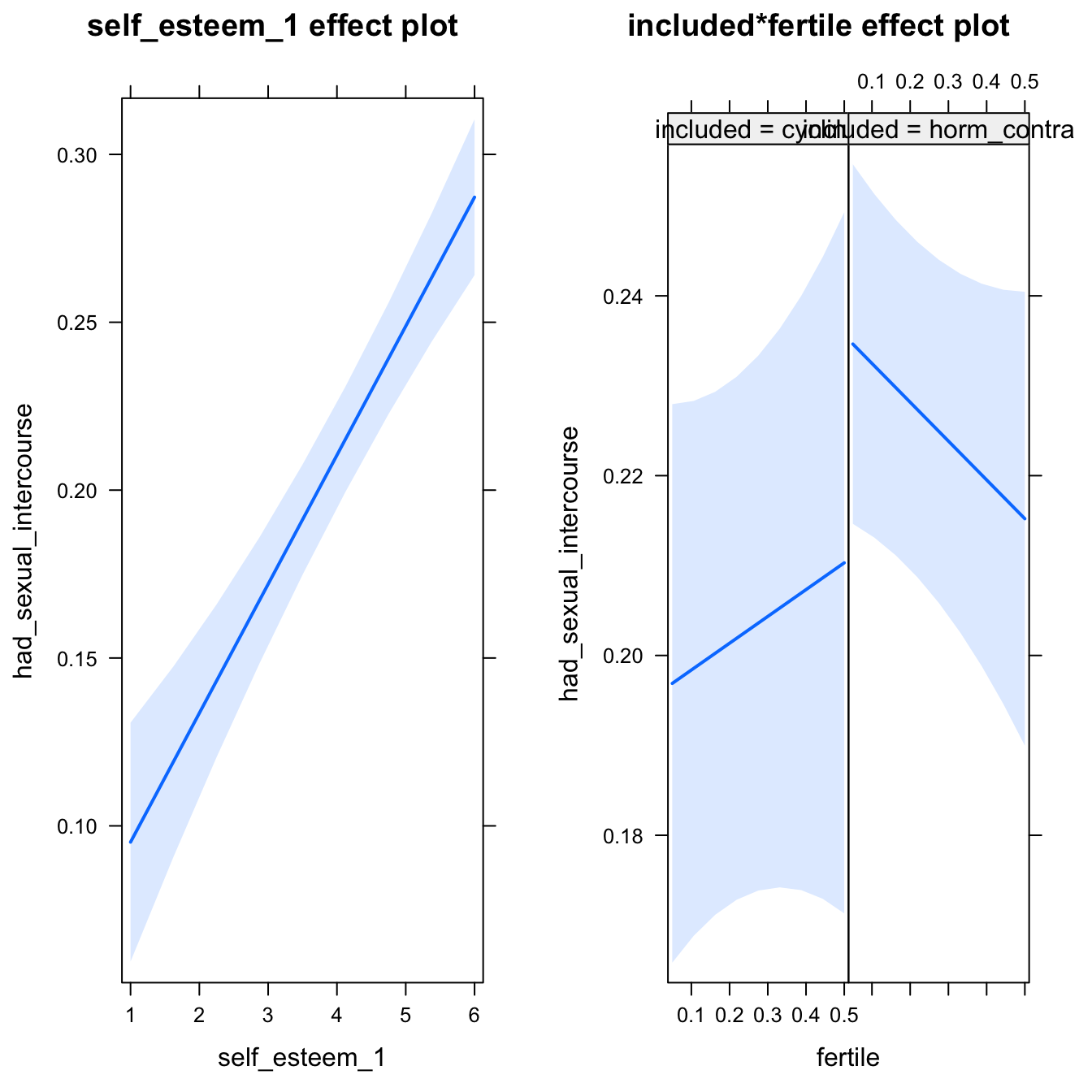
Broad window
outcome = names(model@frame)[1]
broad_models[[outcome]] <<- model %>%
  switch_window_to_broad(diary)
Generalized linear mixed model fit by maximum likelihood (Laplace Approximation) ['glmerMod']
Family: binomial ( probit )
Formula: had_sexual_intercourse ~ included * fertile + (1 | person)
Data: diary2
AIC BIC logLik deviance df.resid
7763 7798 -3876 7753 7740
Scaled residuals:
Min 1Q Median 3Q Max
-1.809 -0.538 -0.397 -0.245 3.461
Random effects:
Groups Name Variance Std.Dev.
person (Intercept) 0.268 0.518
Number of obs: 7745, groups: person, 493
Fixed effects:
Estimate Std. Error z value Pr(>|z|)
(Intercept) -0.9906 0.0677 -14.64 <2e-16 ***
includedhorm_contra 0.1763 0.0791 2.23 0.026 *
fertile 0.0767 0.1715 0.45 0.654
includedhorm_contra:fertile -0.2240 0.2023 -1.11 0.268
---
Signif. codes: 0 '***' 0.001 '**' 0.01 '*' 0.05 '.' 0.1 ' ' 1
Correlation of Fixed Effects:
(Intr) incld_ fertil
inclddhrm_c -0.846
fertile -0.541 0.463
inclddhrm_: 0.460 -0.546 -0.848
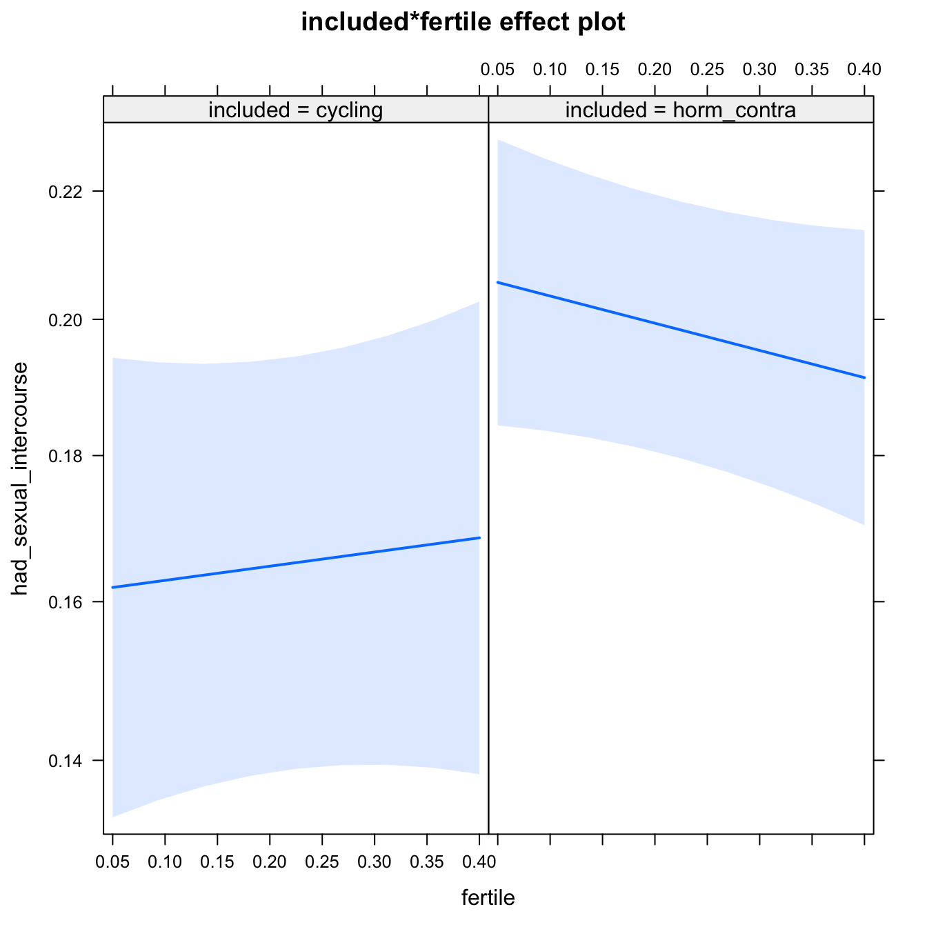
Diagnostics
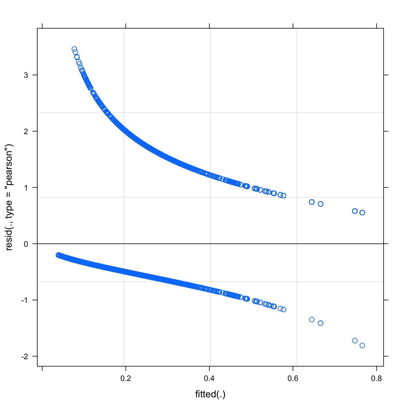
## Warning: 'sjp.lmer' is deprecated.
## Use 'plot_model' instead.
## See help("Deprecated")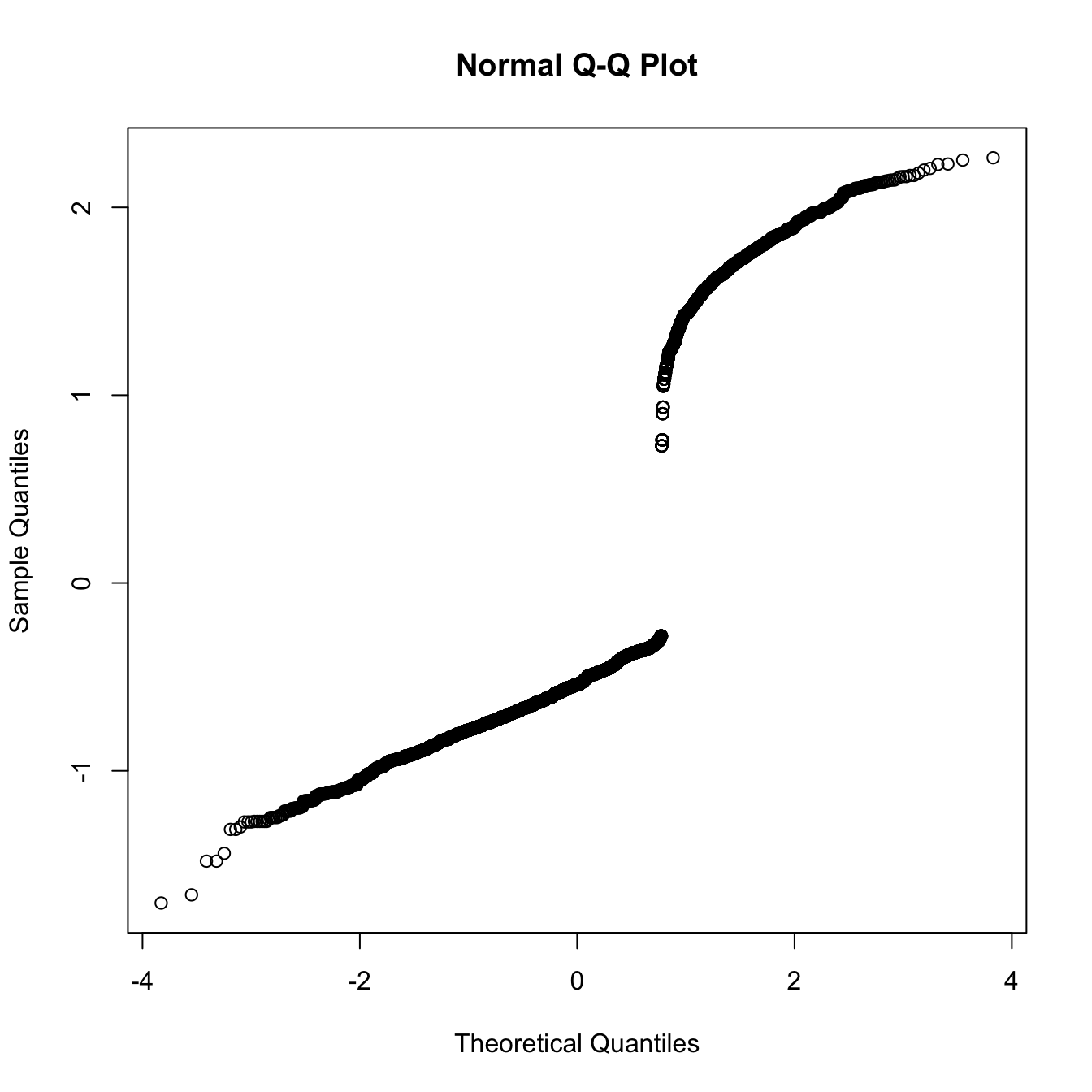
## Warning: 'sjp.lmer' is deprecated.
## Use 'plot_model' instead.
## See help("Deprecated")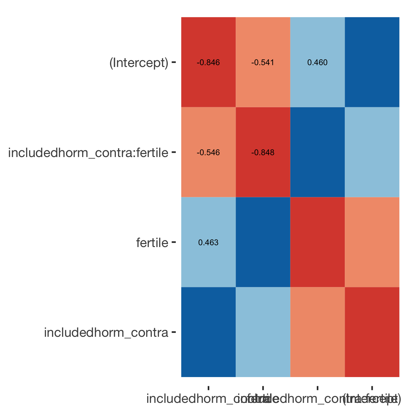
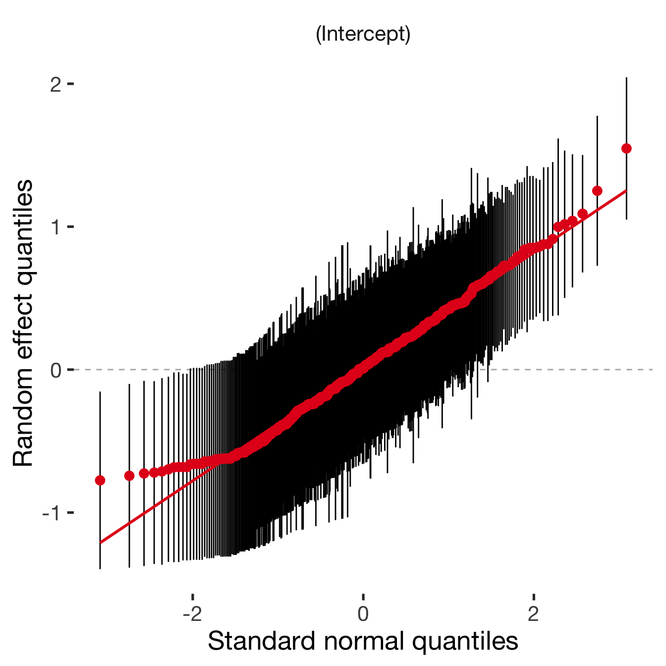
Adjusting for self esteem
broad_models[[outcome]] %>%
  adjust_for_self_esteem(diary2)
##
##
## ```
## Linear mixed model fit by REML. t-tests use Satterthwaite's method ['lmerModLmerTest']
## Formula: form
## Data: diary
##
## REML criterion at convergence: 7844
##
## Scaled residuals:
## Min 1Q Median 3Q Max
## -1.913 -0.608 -0.367 -0.085 2.566
##
## Random effects:
## Groups Name Variance Std.Dev.
## person (Intercept) 0.0187 0.137
## Residual 0.1503 0.388
## Number of obs: 7741, groups: person, 493
##
## Fixed effects:
## Estimate Std. Error df t value Pr(>|t|)
## (Intercept) 0.03581 0.02609 2354.11996 1.37 0.170
## includedhorm_contra 0.04043 0.02019 949.13044 2.00 0.046 *
## fertile 0.01863 0.04312 7512.46279 0.43 0.666
## self_esteem_1 0.03775 0.00461 5396.96418 8.20 3.1e-16 ***
## includedhorm_contra:fertile -0.06403 0.05147 7529.69338 -1.24 0.214
## ---
## Signif. codes: 0 '***' 0.001 '**' 0.01 '*' 0.05 '.' 0.1 ' ' 1
##
## Correlation of Fixed Effects:
## (Intr) incld_ fertil slf__1
## inclddhrm_c -0.562
## fertile -0.344 0.452
## self_estm_1 -0.760 0.021 -0.008
## inclddhrm_: 0.295 -0.542 -0.838 -0.002
##
## ```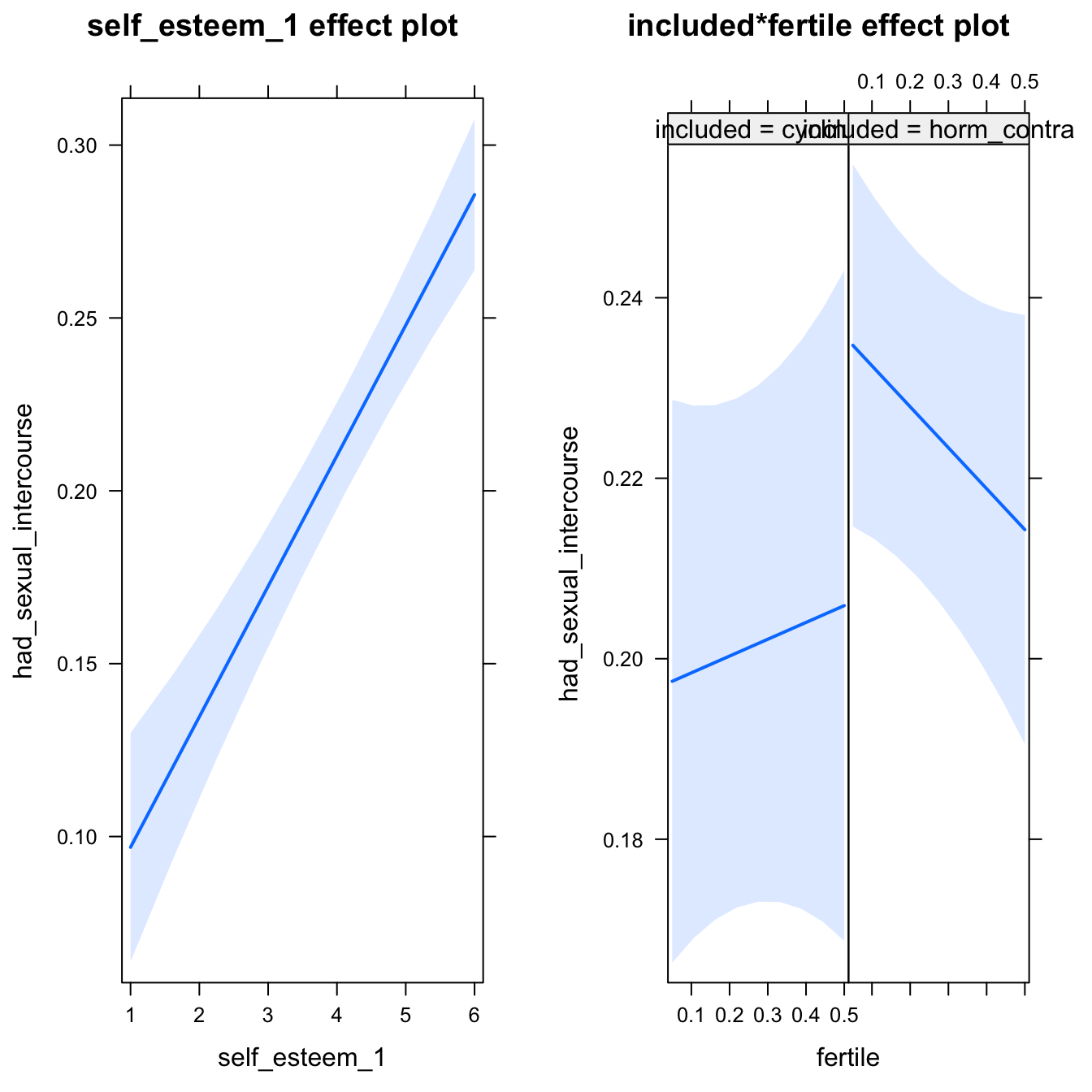
bla = 2do_moderators(models$had_sexual_intercourse, diary)Moderators
H2_1 Partner’s physical attractiveness
Predicted fertile phase effect sizes (in red): biggest (EP desire, partner mate retention)/smallest (IP desire) when partner’s physical attractiveness is low.
model %>%
  test_moderator("partner_attractiveness_physical", diary)
## Warning in checkConv(attr(opt, "derivs"), opt$par, ctrl = control$checkConv, : Model failed to converge with
## max|grad| = 0.00281528 (tol = 0.001, component 1)## Warning in checkConv(attr(opt, "derivs"), opt$par, ctrl = control$checkConv, : Model failed to converge with
## max|grad| = 0.404656 (tol = 0.001, component 1)| Df | AIC | BIC | logLik | deviance | Chisq | Chi Df | Pr(>Chisq) | |
|---|---|---|---|---|---|---|---|---|
| with_main | 7 | 6453 | 6500 | -3219 | 6439 | NA | NA | NA |
| with_mod | 9 | 6456 | 6517 | -3219 | 6438 | 0.6562 | 2 | 0.7203 |
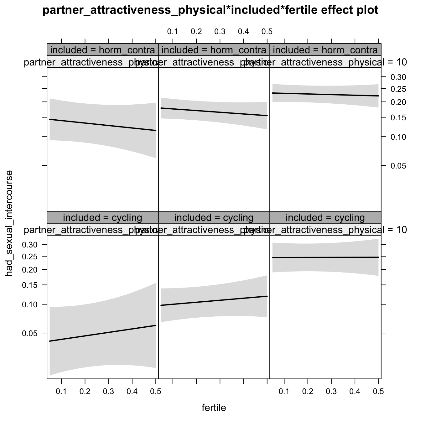
Generalized linear mixed model fit by maximum likelihood (Laplace Approximation) ['glmerMod']
 Family: binomial  ( probit )
Formula: had_sexual_intercourse ~ (1 | person) + partner_attractiveness_physical +
    included + fertile + partner_attractiveness_physical:included +
    partner_attractiveness_physical:fertile + included:fertile +
    partner_attractiveness_physical:included:fertile
   Data: diary

     AIC      BIC   logLik deviance df.resid
    6456     6517    -3219     6438     6374

Scaled residuals:
   Min     1Q Median     3Q    Max
-1.481 -0.530 -0.401 -0.254  3.638

Random effects:
 Groups Name        Variance Std.Dev.
 person (Intercept) 0.231    0.481
Number of obs: 6383, groups:  person, 493

Fixed effects:
                                                            Estimate Std. Error z value      Pr(>|z|)
(Intercept)                                                  -2.2316     0.3634   -6.14 0.00000000082 ***
partner_attractiveness_physical                               0.1541     0.0436    3.53       0.00041 ***
includedhorm_contra                                           1.0467     0.4246    2.47       0.01369 *
fertile                                                       0.6270     0.9543    0.66       0.51114
partner_attractiveness_physical:includedhorm_contra          -0.1082     0.0509   -2.12       0.03373 *
partner_attractiveness_physical:fertile                      -0.0620     0.1141   -0.54       0.58669
includedhorm_contra:fertile                                  -1.0384     1.1357   -0.91       0.36057
partner_attractiveness_physical:includedhorm_contra:fertile   0.0951     0.1356    0.70       0.48317
---
Signif. codes:  0 '***' 0.001 '**' 0.01 '*' 0.05 '.' 0.1 ' ' 1

Correlation of Fixed Effects:
            (Intr) prtn__ incld_ fertil pr__:_ prt__: incl_:
prtnr_ttrc_ -0.984
inclddhrm_c -0.854  0.841
fertile     -0.521  0.510  0.445
prtnr_tt_:_  0.841 -0.855 -0.984 -0.436
prtnr_ttr_:  0.512 -0.517 -0.438 -0.984  0.442
inclddhrm_:  0.438 -0.428 -0.516 -0.839  0.505  0.826
prtnr_t_:_: -0.430  0.435  0.507  0.827 -0.512 -0.840 -0.984
convergence code: 0
Model failed to converge with max|grad| = 0.404656 (tol = 0.001, component 1)
H2_1 Partner’s short-term attractiveness
Predicted fertile phase effect sizes (in red): biggest (EP desire, partner mate retention)/smallest (IP desire) when partner’s short-term attractiveness is low.
model %>%
test_moderator("partner_attractiveness_shortterm", diary)| Df | AIC | BIC | logLik | deviance | Chisq | Chi Df | Pr(>Chisq) | |
|---|---|---|---|---|---|---|---|---|
| with_main | 7 | 6430 | 6478 | -3208 | 6416 | NA | NA | NA |
| with_mod | 9 | 6431 | 6492 | -3206 | 6413 | 3.251 | 2 | 0.1968 |

Generalized linear mixed model fit by maximum likelihood (Laplace Approximation) ['glmerMod']
 Family: binomial  ( probit )
Formula: had_sexual_intercourse ~ (1 | person) + partner_attractiveness_shortterm +
    included + fertile + partner_attractiveness_shortterm:included +
    partner_attractiveness_shortterm:fertile + included:fertile +
    partner_attractiveness_shortterm:included:fertile
   Data: diary

     AIC      BIC   logLik deviance df.resid
    6431     6492    -3206     6413     6374

Scaled residuals:
   Min     1Q Median     3Q    Max
-1.427 -0.535 -0.404 -0.235  4.365

Random effects:
 Groups Name        Variance Std.Dev.
 person (Intercept) 0.216    0.465
Number of obs: 6383, groups:  person, 493

Fixed effects:
                                                             Estimate Std. Error z value    Pr(>|z|)
(Intercept)                                                   -0.9867     0.0650  -15.18     < 2e-16 ***
partner_attractiveness_shortterm                               0.3821     0.0711    5.37 0.000000078 ***
includedhorm_contra                                            0.1614     0.0758    2.13      0.0332 *
fertile                                                        0.1508     0.1705    0.88      0.3765
partner_attractiveness_shortterm:includedhorm_contra          -0.2554     0.0821   -3.11      0.0019 **
partner_attractiveness_shortterm:fertile                      -0.3250     0.1849   -1.76      0.0787 .
includedhorm_contra:fertile                                   -0.2976     0.2030   -1.47      0.1426
partner_attractiveness_shortterm:includedhorm_contra:fertile   0.3729     0.2174    1.72      0.0863 .
---
Signif. codes:  0 '***' 0.001 '**' 0.01 '*' 0.05 '.' 0.1 ' ' 1

Correlation of Fixed Effects:
            (Intr) prtn__ incld_ fertil pr__:_ prt__: incl_:
prtnr_ttrc_ -0.100
inclddhrm_c -0.844  0.079
fertile     -0.518  0.080  0.443
prtnr_tt_:_  0.084 -0.865 -0.114 -0.069
prtnr_ttr_:  0.081 -0.547 -0.067 -0.112  0.473
inclddhrm_:  0.436 -0.067 -0.519 -0.840  0.086  0.094
prtnr_t_:_: -0.069  0.465  0.085  0.095 -0.537 -0.850 -0.140
H2_1 Partner’s short-term vs long-term attractiveness
Predicted fertile phase effect sizes (in red): biggest (EP desire, partner mate retention)/smallest (IP desire) top-right (high LT, low ST), then top-left (low LT, low ST), then bottom-left (low LT, high ST), then bottom-right (high LT/ST).
add_main = update.formula(formula(model), new = as.formula(paste0(". ~ . + partner_attractiveness_longterm * included + partner_attractiveness_shortterm * included + partner_attractiveness_longterm * partner_attractiveness_shortterm"))) # reorder so that the triptych looks nice
add_mod_formula = update.formula(update.formula(formula(model), new = . ~ . - included * fertile), new = as.formula(paste0(". ~ . + partner_attractiveness_longterm * fertile * partner_attractiveness_shortterm * included"))) # reorder so that the triptych looks nice

update(model, formula = add_main) -> with_main
## Warning in checkConv(attr(opt, "derivs"), opt$par, ctrl = control$checkConv, : Model failed to converge with
## max|grad| = 0.00696294 (tol = 0.001, component 1)update(model, formula = add_mod_formula) -> with_mod## Warning in checkConv(attr(opt, "derivs"), opt$par, ctrl = control$checkConv, : Model failed to converge with
## max|grad| = 0.00846618 (tol = 0.001, component 1)if (is(with_mod, "lmerMod")) {
with_mod <- as_lmerModLmerTest(with_mod)
}
cat(pander(anova(with_main, with_mod)))| Df | AIC | BIC | logLik | deviance | Chisq | Chi Df | Pr(>Chisq) | |
|---|---|---|---|---|---|---|---|---|
| with_main | 10 | 6429 | 6497 | -3205 | 6409 | NA | NA | NA |
| with_mod | 17 | 6435 | 6550 | -3201 | 6401 | 8.063 | 7 | 0.3271 |
effs = allEffects(with_mod)
effs = data.frame(effs$`partner_attractiveness_longterm:fertile:partner_attractiveness_shortterm:included`) %>%
filter(round(partner_attractiveness_longterm,1) %in% c(-3,-2,0.8),round(partner_attractiveness_shortterm,1) %in% c(-2,0.5, 2))
ggplot(effs, aes(fertile, fit, ymin = lower, ymax = upper, color = included)) +
facet_grid(partner_attractiveness_shortterm ~ partner_attractiveness_longterm) +
geom_smooth(stat='identity') +
scale_color_manual(values = c("cycling" = 'red', 'horm_contra' = 'black'), guide = F) +
scale_fill_manual(values = c("cycling" = 'red', 'horm_contra' = 'black'), guide = F) +
ggtitle("Moderation", "top-to-bottom: short-term,\nleft-to-right: long-term attractiveness of the partner")+
ylab(names(model@frame)[1])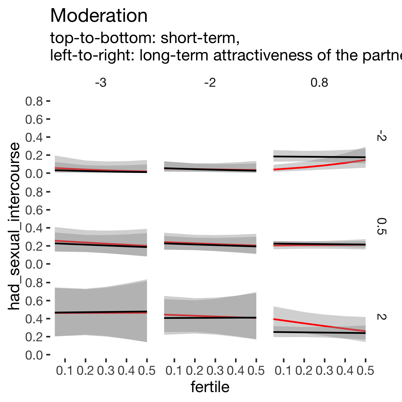
print_summary(with_mod)Generalized linear mixed model fit by maximum likelihood (Laplace Approximation) ['glmerMod']
Family: binomial ( probit )
Formula: had_sexual_intercourse ~ (1 | person) + partner_attractiveness_longterm +
fertile + partner_attractiveness_shortterm + included + partner_attractiveness_longterm:fertile +
partner_attractiveness_longterm:partner_attractiveness_shortterm +
fertile:partner_attractiveness_shortterm + partner_attractiveness_longterm:included +
fertile:included + partner_attractiveness_shortterm:included +
partner_attractiveness_longterm:fertile:partner_attractiveness_shortterm +
partner_attractiveness_longterm:fertile:included + partner_attractiveness_longterm:partner_attractiveness_shortterm:included +
fertile:partner_attractiveness_shortterm:included + partner_attractiveness_longterm:fertile:partner_attractiveness_shortterm:included
Data: diary
AIC BIC logLik deviance df.resid
6435 6550 -3200 6401 6366
Scaled residuals:
Min 1Q Median 3Q Max
-1.435 -0.537 -0.409 -0.221 4.079
Random effects:
Groups Name Variance Std.Dev.
person (Intercept) 0.212 0.46
Number of obs: 6383, groups: person, 493
Fixed effects:
Estimate
(Intercept) -0.9849
partner_attractiveness_longterm -0.0576
fertile 0.1716
partner_attractiveness_shortterm 0.3937
includedhorm_contra 0.1710
partner_attractiveness_longterm:fertile 0.2420
partner_attractiveness_longterm:partner_attractiveness_shortterm 0.0118
fertile:partner_attractiveness_shortterm -0.4137
partner_attractiveness_longterm:includedhorm_contra 0.1011
fertile:includedhorm_contra -0.3283
partner_attractiveness_shortterm:includedhorm_contra -0.2580
partner_attractiveness_longterm:fertile:partner_attractiveness_shortterm -0.2323
partner_attractiveness_longterm:fertile:includedhorm_contra -0.1441
partner_attractiveness_longterm:partner_attractiveness_shortterm:includedhorm_contra -0.1098
fertile:partner_attractiveness_shortterm:includedhorm_contra 0.4654
partner_attractiveness_longterm:fertile:partner_attractiveness_shortterm:includedhorm_contra 0.1637
Std. Error
(Intercept) 0.0656
partner_attractiveness_longterm 0.0669
fertile 0.1730
partner_attractiveness_shortterm 0.0751
includedhorm_contra 0.0769
partner_attractiveness_longterm:fertile 0.1867
partner_attractiveness_longterm:partner_attractiveness_shortterm 0.0584
fertile:partner_attractiveness_shortterm 0.1938
partner_attractiveness_longterm:includedhorm_contra 0.0840
fertile:includedhorm_contra 0.2073
partner_attractiveness_shortterm:includedhorm_contra 0.0866
partner_attractiveness_longterm:fertile:partner_attractiveness_shortterm 0.1682
partner_attractiveness_longterm:fertile:includedhorm_contra 0.2373
partner_attractiveness_longterm:partner_attractiveness_shortterm:includedhorm_contra 0.0797
fertile:partner_attractiveness_shortterm:includedhorm_contra 0.2299
partner_attractiveness_longterm:fertile:partner_attractiveness_shortterm:includedhorm_contra 0.2333
z value
(Intercept) -15.01
partner_attractiveness_longterm -0.86
fertile 0.99
partner_attractiveness_shortterm 5.25
includedhorm_contra 2.22
partner_attractiveness_longterm:fertile 1.30
partner_attractiveness_longterm:partner_attractiveness_shortterm 0.20
fertile:partner_attractiveness_shortterm -2.13
partner_attractiveness_longterm:includedhorm_contra 1.20
fertile:includedhorm_contra -1.58
partner_attractiveness_shortterm:includedhorm_contra -2.98
partner_attractiveness_longterm:fertile:partner_attractiveness_shortterm -1.38
partner_attractiveness_longterm:fertile:includedhorm_contra -0.61
partner_attractiveness_longterm:partner_attractiveness_shortterm:includedhorm_contra -1.38
fertile:partner_attractiveness_shortterm:includedhorm_contra 2.02
partner_attractiveness_longterm:fertile:partner_attractiveness_shortterm:includedhorm_contra 0.70
Pr(>|z|)
(Intercept) < 2e-16 ***
partner_attractiveness_longterm 0.3891
fertile 0.3210
partner_attractiveness_shortterm 0.00000016 ***
includedhorm_contra 0.0262 *
partner_attractiveness_longterm:fertile 0.1948
partner_attractiveness_longterm:partner_attractiveness_shortterm 0.8401
fertile:partner_attractiveness_shortterm 0.0328 *
partner_attractiveness_longterm:includedhorm_contra 0.2286
fertile:includedhorm_contra 0.1133
partner_attractiveness_shortterm:includedhorm_contra 0.0029 **
partner_attractiveness_longterm:fertile:partner_attractiveness_shortterm 0.1673
partner_attractiveness_longterm:fertile:includedhorm_contra 0.5436
partner_attractiveness_longterm:partner_attractiveness_shortterm:includedhorm_contra 0.1683
fertile:partner_attractiveness_shortterm:includedhorm_contra 0.0429 *
partner_attractiveness_longterm:fertile:partner_attractiveness_shortterm:includedhorm_contra 0.4831
---
Signif. codes: 0 '***' 0.001 '**' 0.01 '*' 0.05 '.' 0.1 ' ' 1
convergence code: 0
Model failed to converge with max|grad| = 0.00846618 (tol = 0.001, component 1)
H2_1b Partner’s short-term and long-term attractiveness
Edit: Alternative model specification, added after publication. Predicted fertile phase effect sizes (in red): biggest (EP desire, partner mate retention)/smallest (IP desire) top-right (high LT, low ST), then top-left (low LT, low ST), then bottom-left (low LT, high ST), then bottom-right (high LT/ST).
add_main = update.formula(formula(model), new = as.formula(paste0(". ~ . + partner_attractiveness_shortterm * included + partner_attractiveness_longterm * fertile * included"))) # reorder so that the triptych looks nice
add_mod_formula = update.formula(update.formula(formula(model), new = . ~ . - included * fertile), new = as.formula(paste0(". ~ . + (partner_attractiveness_shortterm + partner_attractiveness_longterm) * fertile * included"))) # reorder so that the triptych looks nice
update(model, formula = add_main) -> with_main## Warning in checkConv(attr(opt, "derivs"), opt$par, ctrl = control$checkConv, : Model failed to converge with
## max|grad| = 0.0016579 (tol = 0.001, component 1)update(model, formula = add_mod_formula) -> with_mod## Warning in checkConv(attr(opt, "derivs"), opt$par, ctrl = control$checkConv, : Model failed to converge with
## max|grad| = 0.0184226 (tol = 0.001, component 1)if (is(with_mod, "lmerMod")) {
with_mod <- as_lmerModLmerTest(with_mod)
}
cat(pander(anova(with_main, with_mod)))| Df | AIC | BIC | logLik | deviance | Chisq | Chi Df | Pr(>Chisq) | |
|---|---|---|---|---|---|---|---|---|
| with_main | 11 | 6435 | 6509 | -3206 | 6413 | NA | NA | NA |
| with_mod | 13 | 6435 | 6523 | -3205 | 6409 | 3.704 | 2 | 0.1569 |
plot_triptych(with_mod)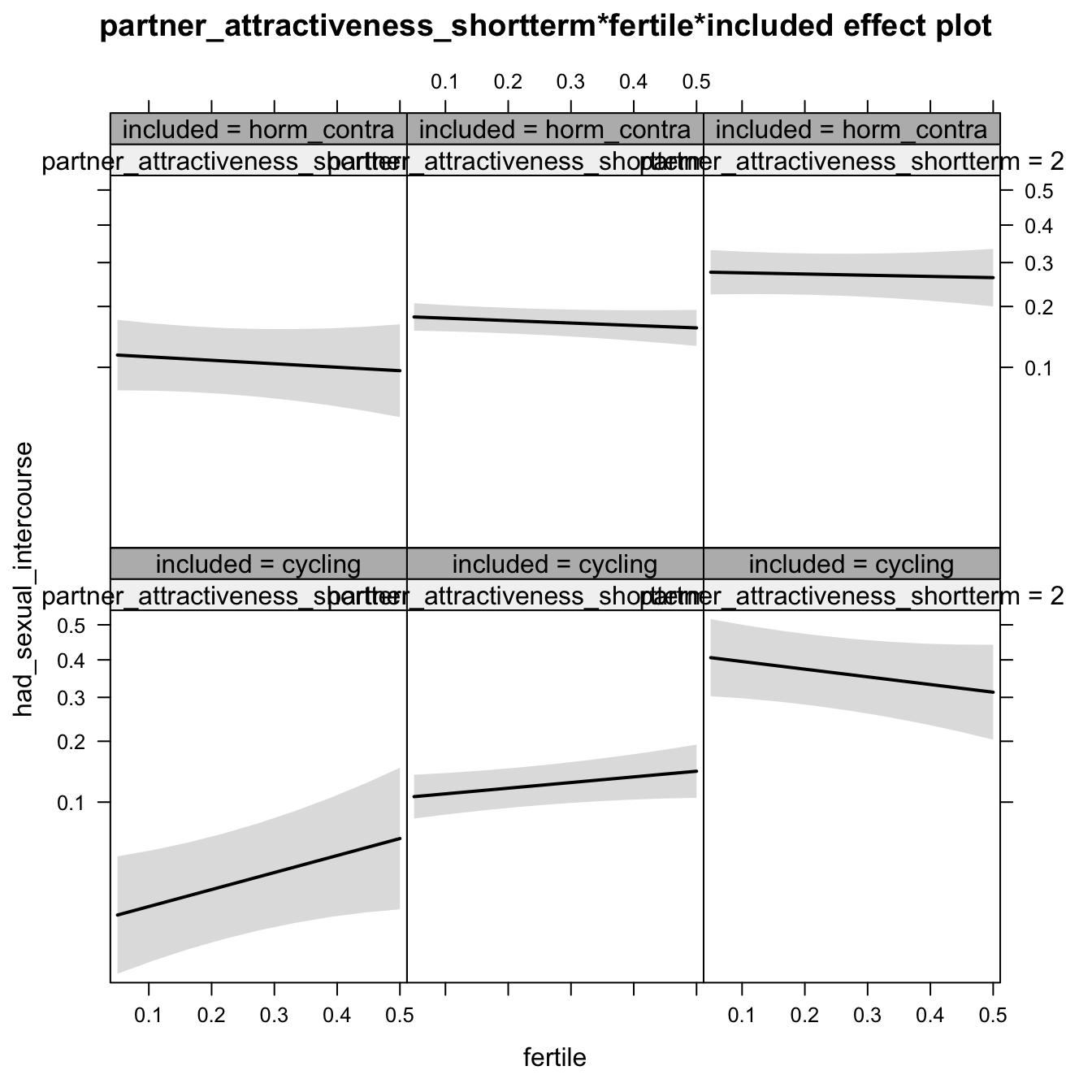
print_summary(with_mod)Generalized linear mixed model fit by maximum likelihood (Laplace Approximation) ['glmerMod']
Family: binomial ( probit )
Formula: had_sexual_intercourse ~ (1 | person) + partner_attractiveness_shortterm +
partner_attractiveness_longterm + fertile + included + partner_attractiveness_shortterm:fertile +
partner_attractiveness_longterm:fertile + partner_attractiveness_shortterm:included +
partner_attractiveness_longterm:included + fertile:included +
partner_attractiveness_shortterm:fertile:included + partner_attractiveness_longterm:fertile:included
Data: diary
AIC BIC logLik deviance df.resid
6435 6523 -3205 6409 6370
Scaled residuals:
Min 1Q Median 3Q Max
-1.427 -0.537 -0.407 -0.237 4.183
Random effects:
Groups Name Variance Std.Dev.
person (Intercept) 0.216 0.464
Number of obs: 6383, groups: person, 493
Fixed effects:
Estimate Std. Error z value Pr(>|z|)
(Intercept) -0.9845 0.0650 -15.15 < 2e-16 ***
partner_attractiveness_shortterm 0.3899 0.0719 5.42 0.000000059 ***
partner_attractiveness_longterm -0.0501 0.0667 -0.75 0.4528
fertile 0.1391 0.1710 0.81 0.4159
includedhorm_contra 0.1539 0.0760 2.02 0.0430 *
partner_attractiveness_shortterm:fertile -0.3566 0.1875 -1.90 0.0571 .
partner_attractiveness_longterm:fertile 0.1974 0.1815 1.09 0.2769
partner_attractiveness_shortterm:includedhorm_contra -0.2718 0.0833 -3.26 0.0011 **
partner_attractiveness_longterm:includedhorm_contra 0.0971 0.0839 1.16 0.2473
fertile:includedhorm_contra -0.3014 0.2047 -1.47 0.1409
partner_attractiveness_shortterm:fertile:includedhorm_contra 0.3895 0.2209 1.76 0.0778 .
partner_attractiveness_longterm:fertile:includedhorm_contra -0.1009 0.2330 -0.43 0.6649
---
Signif. codes: 0 '***' 0.001 '**' 0.01 '*' 0.05 '.' 0.1 ' ' 1
Correlation of Fixed Effects:
(Intr) prtnr_ttrctvnss_s prtnr_ttrctvnss_l fertil incld_ prtnr_ttrctvnss_s:
prtnr_ttrctvnss_s -0.090
prtnr_ttrctvnss_l -0.038 -0.170
fertile -0.517 0.076 0.013
inclddhrm_c -0.841 0.070 0.031 0.440
prtnr_ttrctvnss_s: 0.076 -0.542 0.082 -0.102 -0.063
prtnr_ttrctvnss_l: 0.014 0.075 -0.500 -0.065 -0.012 -0.159
prtnr_ttrctvnss_s:_ 0.076 -0.863 0.147 -0.065 -0.097 0.468
prtnr_ttrctvnss_l:_ 0.027 0.136 -0.795 -0.010 -0.076 -0.065
frtl:ncldd_ 0.433 -0.064 -0.011 -0.836 -0.518 0.085
prtnr_ttrctvnss_s::_ -0.064 0.460 -0.069 0.086 0.076 -0.849
prtnr_ttrctvnss_l::_ -0.012 -0.058 0.390 0.051 0.039 0.124
prtnr_ttrctvnss_l: prtnr_ttrctvnss_s:_ prtnr_ttrctvnss_l:_ frtl:_ prtnr_ttrctvnss_s::_
prtnr_ttrctvnss_s
prtnr_ttrctvnss_l
fertile
inclddhrm_c
prtnr_ttrctvnss_s:
prtnr_ttrctvnss_l:
prtnr_ttrctvnss_s:_ -0.065
prtnr_ttrctvnss_l:_ 0.397 -0.182
frtl:ncldd_ 0.055 0.077 0.040
prtnr_ttrctvnss_s::_ 0.135 -0.534 0.090 -0.120
prtnr_ttrctvnss_l::_ -0.779 0.083 -0.502 -0.111 -0.171
convergence code: 0
Model failed to converge with max|grad| = 0.0184226 (tol = 0.001, component 1)
H2_1c Partner’s short-term minus long-term attractiveness
Edit: Alternative model specification, added after publication. Predicted fertile phase effect sizes (in red): biggest (EP desire, partner mate retention)/smallest (IP desire) top-right (high LT, low ST), then top-left (low LT, low ST), then bottom-left (low LT, high ST), then bottom-right (high LT/ST).
add_main = update.formula(formula(model), new = as.formula(paste0(". ~ . + partner_st_vs_lt * included"))) # reorder so that the triptych looks nice
add_mod_formula = update.formula(update.formula(formula(model), new = . ~ . - included * fertile), new = as.formula(paste0(". ~ . + partner_st_vs_lt * fertile * included"))) # reorder so that the triptych looks nice
update(model, formula = add_main) -> with_main
update(model, formula = add_mod_formula) -> with_mod## Warning in checkConv(attr(opt, "derivs"), opt$par, ctrl = control$checkConv, : Model failed to converge with
## max|grad| = 0.00808856 (tol = 0.001, component 1)if (is(with_mod, "lmerMod")) {
with_mod <- as_lmerModLmerTest(with_mod)
}
cat(pander(anova(with_main, with_mod)))| Df | AIC | BIC | logLik | deviance | Chisq | Chi Df | Pr(>Chisq) | |
|---|---|---|---|---|---|---|---|---|
| with_main | 7 | 6458 | 6506 | -3222 | 6444 | NA | NA | NA |
| with_mod | 9 | 6459 | 6520 | -3220 | 6441 | 3.405 | 2 | 0.1822 |
plot_triptych(with_mod)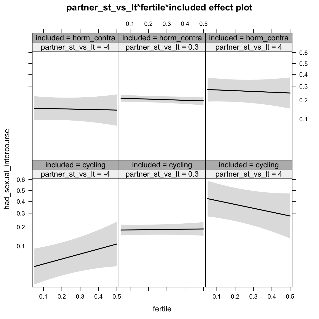
print_summary(with_mod)Generalized linear mixed model fit by maximum likelihood (Laplace Approximation) ['glmerMod']
Family: binomial ( probit )
Formula: had_sexual_intercourse ~ (1 | person) + partner_st_vs_lt + fertile +
included + partner_st_vs_lt:fertile + partner_st_vs_lt:included +
fertile:included + partner_st_vs_lt:fertile:included
Data: diary
AIC BIC logLik deviance df.resid
6459 6520 -3220 6441 6374
Scaled residuals:
Min 1Q Median 3Q Max
-1.469 -0.529 -0.404 -0.262 3.571
Random effects:
Groups Name Variance Std.Dev.
person (Intercept) 0.236 0.485
Number of obs: 6383, groups: person, 493
Fixed effects:
Estimate Std. Error z value Pr(>|z|)
(Intercept) -0.9781 0.0656 -14.91 < 2e-16 ***
partner_st_vs_lt 0.2085 0.0534 3.90 0.000095 ***
fertile 0.1325 0.1693 0.78 0.434
includedhorm_contra 0.1677 0.0764 2.20 0.028 *
partner_st_vs_lt:fertile -0.2552 0.1392 -1.83 0.067 .
partner_st_vs_lt:includedhorm_contra -0.1541 0.0645 -2.39 0.017 *
fertile:includedhorm_contra -0.2689 0.2007 -1.34 0.180
partner_st_vs_lt:fertile:includedhorm_contra 0.2451 0.1708 1.43 0.151
---
Signif. codes: 0 '***' 0.001 '**' 0.01 '*' 0.05 '.' 0.1 ' ' 1
Correlation of Fixed Effects:
(Intr) prt___ fertil incld_ pr___: p___:_ frtl:_
prtnr_st_v_ -0.022
fertile -0.503 0.033
inclddhrm_c -0.846 0.015 0.432
prtnr_st__: 0.034 -0.502 -0.019 -0.028
prtnr_s__:_ 0.018 -0.828 -0.027 -0.016 0.416
frtl:ncldd_ 0.426 -0.028 -0.844 -0.506 0.016 0.025
prtnr___::_ -0.027 0.409 0.015 0.025 -0.815 -0.502 -0.018
convergence code: 0
Model failed to converge with max|grad| = 0.00808856 (tol = 0.001, component 1)
H2_3 Relative attractiveness to self
Predicted fertile phase effect sizes (in red): biggest (EP desire, partner mate retention)/smallest (IP desire) when partner’s relative attractiveness is low.
model %>%
test_moderator("partner_attractiveness_rel_to_self", diary)## Warning in checkConv(attr(opt, "derivs"), opt$par, ctrl = control$checkConv, : Model failed to converge with
## max|grad| = 0.00415496 (tol = 0.001, component 1)| Df | AIC | BIC | logLik | deviance | Chisq | Chi Df | Pr(>Chisq) | |
|---|---|---|---|---|---|---|---|---|
| with_main | 7 | 6471 | 6519 | -3229 | 6457 | NA | NA | NA |
| with_mod | 9 | 6472 | 6533 | -3227 | 6454 | 3.635 | 2 | 0.1624 |
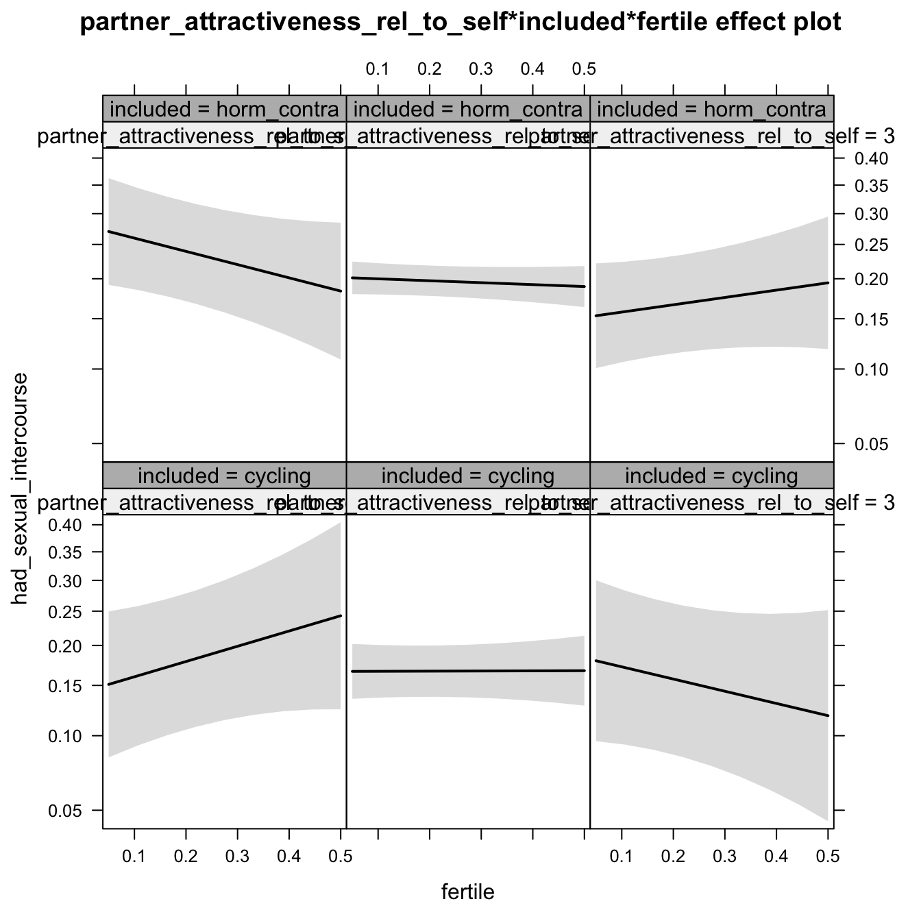
Generalized linear mixed model fit by maximum likelihood (Laplace Approximation) ['glmerMod']
Family: binomial ( probit )
Formula: had_sexual_intercourse ~ (1 | person) + partner_attractiveness_rel_to_self +
included + fertile + partner_attractiveness_rel_to_self:included +
partner_attractiveness_rel_to_self:fertile + included:fertile +
partner_attractiveness_rel_to_self:included:fertile
Data: diary
AIC BIC logLik deviance df.resid
6472 6533 -3227 6454 6374
Scaled residuals:
Min 1Q Median 3Q Max
-1.639 -0.528 -0.401 -0.262 3.272
Random effects:
Groups Name Variance Std.Dev.
person (Intercept) 0.248 0.498
Number of obs: 6383, groups: person, 493
Fixed effects:
Estimate Std. Error z value Pr(>|z|)
(Intercept) -0.9776 0.0669 -14.62 <2e-16 ***
partner_attractiveness_rel_to_self 0.0304 0.0639 0.48 0.634
includedhorm_contra 0.1681 0.0777 2.16 0.031 *
fertile 0.0744 0.1729 0.43 0.667
partner_attractiveness_rel_to_self:includedhorm_contra -0.1072 0.0779 -1.38 0.169
partner_attractiveness_rel_to_self:fertile -0.2231 0.1741 -1.28 0.200
includedhorm_contra:fertile -0.2186 0.2039 -1.07 0.284
partner_attractiveness_rel_to_self:includedhorm_contra:fertile 0.3901 0.2106 1.85 0.064 .
---
Signif. codes: 0 '***' 0.001 '**' 0.01 '*' 0.05 '.' 0.1 ' ' 1
Correlation of Fixed Effects:
(Intr) pr____ incld_ fertil pr____:_ pr____: incl_:
prtnr_tt___ 0.157
inclddhrm_c -0.848 -0.136
fertile -0.493 -0.088 0.423
prtnr____:_ -0.128 -0.821 0.100 0.072
prtnr_t___: -0.081 -0.496 0.071 0.202 0.407
inclddhrm_: 0.419 0.075 -0.497 -0.848 -0.055 -0.172
prtn____:_: 0.064 0.410 -0.052 -0.167 -0.498 -0.827 0.126
convergence code: 0
Model failed to converge with max|grad| = 0.00415496 (tol = 0.001, component 1)
H1.3. Cohabitation
diary$cohabitation = factor(diary$cohabitation, c("Long-distance", "Live in same city", "Live in same apartment"))
models$had_sexual_intercourse %>%
test_moderator("cohabitation", diary)## Warning in checkConv(attr(opt, "derivs"), opt$par, ctrl = control$checkConv, : Model failed to converge with
## max|grad| = 0.0159734 (tol = 0.001, component 1)| Df | AIC | BIC | logLik | deviance | Chisq | Chi Df | Pr(>Chisq) | |
|---|---|---|---|---|---|---|---|---|
| with_main | 9 | 6452 | 6513 | -3217 | 6434 | NA | NA | NA |
| with_mod | 13 | 6448 | 6536 | -3211 | 6422 | 11.63 | 4 | 0.02033 |
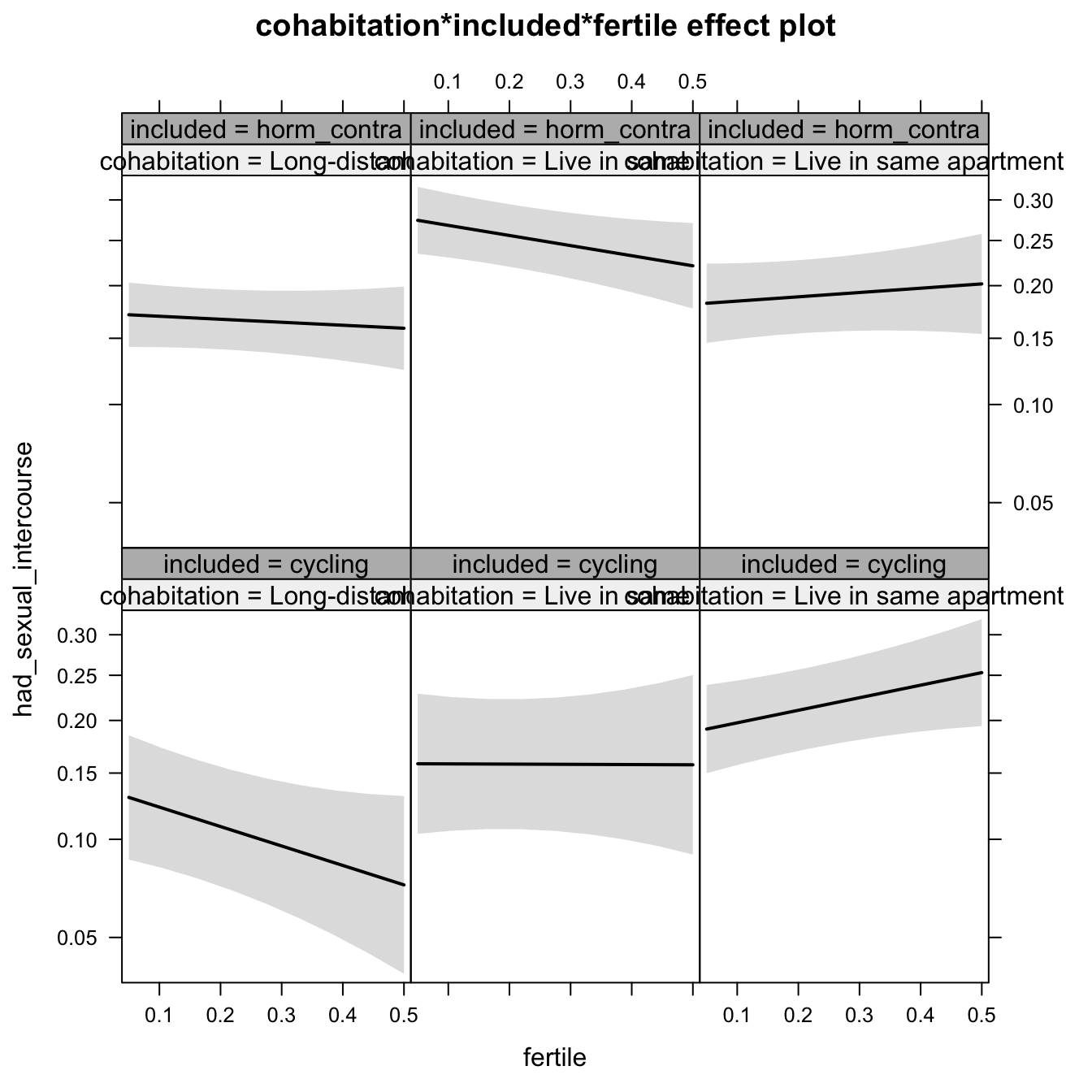
Generalized linear mixed model fit by maximum likelihood (Laplace Approximation) ['glmerMod']
Family: binomial ( probit )
Formula: had_sexual_intercourse ~ (1 | person) + cohabitation + included +
fertile + cohabitation:included + cohabitation:fertile +
included:fertile + cohabitation:included:fertile
Data: diary
AIC BIC logLik deviance df.resid
6448 6536 -3211 6422 6370
Scaled residuals:
Min 1Q Median 3Q Max
-1.630 -0.528 -0.407 -0.257 3.834
Random effects:
Groups Name Variance Std.Dev.
person (Intercept) 0.229 0.478
Number of obs: 6383, groups: person, 493
Fixed effects:
Estimate Std. Error z value Pr(>|z|)
(Intercept) -1.0905 0.1252 -8.71 <2e-16 ***
cohabitationLive in same city 0.0889 0.1880 0.47 0.6361
cohabitationLive in same apartment 0.1936 0.1525 1.27 0.2042
includedhorm_contra 0.1467 0.1402 1.05 0.2953
fertile -0.7196 0.3741 -1.92 0.0544 .
cohabitationLive in same city:includedhorm_contra 0.2738 0.2096 1.31 0.1914
cohabitationLive in same apartment:includedhorm_contra -0.1646 0.1835 -0.90 0.3698
cohabitationLive in same city:fertile 0.7112 0.5346 1.33 0.1834
cohabitationLive in same apartment:fertile 1.1841 0.4352 2.72 0.0065 **
includedhorm_contra:fertile 0.6087 0.4133 1.47 0.1408
cohabitationLive in same city:includedhorm_contra:fertile -0.9746 0.5903 -1.65 0.0987 .
cohabitationLive in same apartment:includedhorm_contra:fertile -0.9140 0.5151 -1.77 0.0760 .
---
Signif. codes: 0 '***' 0.001 '**' 0.01 '*' 0.05 '.' 0.1 ' ' 1
Correlation of Fixed Effects:
(Intr) chLisc chLisa incld_ fertil chLisc:_ chLisa:_ chLisc: chLisa: incl_: cLisc:_:
chbttnLvisc -0.660
chbttnLvisa -0.815 0.541
inclddhrm_c -0.887 0.588 0.726
fertile -0.480 0.320 0.395 0.429
chbttLisc:_ 0.590 -0.896 -0.484 -0.667 -0.287
chbttLisa:_ 0.677 -0.449 -0.831 -0.764 -0.328 0.510
chbttnLisc: 0.335 -0.499 -0.276 -0.300 -0.699 0.448 0.229
chbttnLisa: 0.412 -0.275 -0.489 -0.369 -0.860 0.247 0.407 0.601
inclddhrm_: 0.434 -0.290 -0.357 -0.488 -0.905 0.326 0.373 0.633 0.778
chbtLisc:_: -0.302 0.452 0.249 0.340 0.634 -0.500 -0.260 -0.906 -0.545 -0.700
chbtLisa:_: -0.350 0.233 0.414 0.392 0.726 -0.262 -0.496 -0.508 -0.845 -0.802 0.561
convergence code: 0
Model failed to converge with max|grad| = 0.0159734 (tol = 0.001, component 1)
broad_models$had_sexual_intercourse %>%
test_moderator("cohabitation", diary)## Warning in checkConv(attr(opt, "derivs"), opt$par, ctrl = control$checkConv, : Model failed to converge with
## max|grad| = 0.00579762 (tol = 0.001, component 1)## Warning in checkConv(attr(opt, "derivs"), opt$par, ctrl = control$checkConv, : Model failed to converge with
## max|grad| = 0.0429603 (tol = 0.001, component 1)| Df | AIC | BIC | logLik | deviance | Chisq | Chi Df | Pr(>Chisq) | |
|---|---|---|---|---|---|---|---|---|
| with_main | 9 | 7737 | 7800 | -3860 | 7719 | NA | NA | NA |
| with_mod | 13 | 7737 | 7827 | -3855 | 7711 | 8.51 | 4 | 0.07459 |
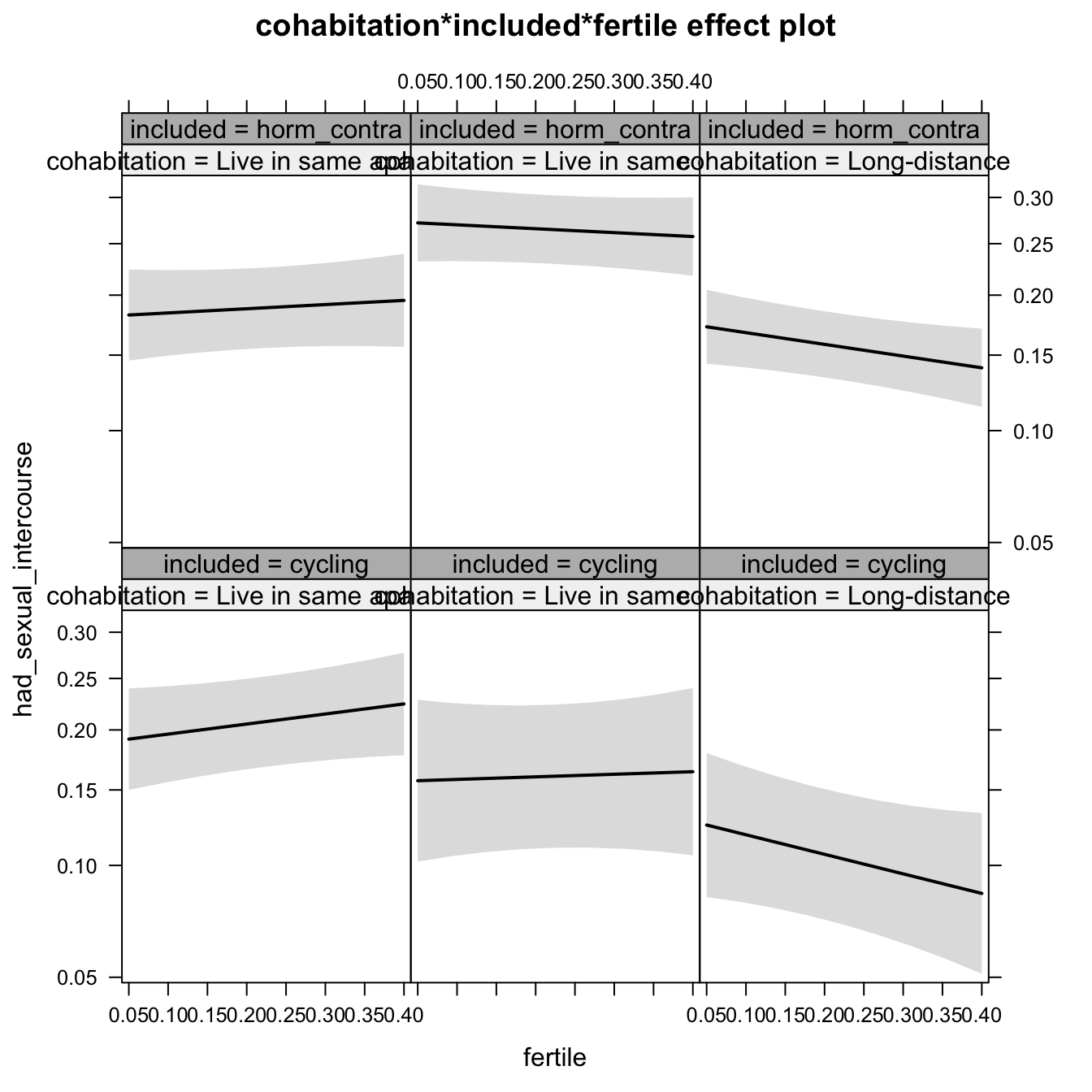
Generalized linear mixed model fit by maximum likelihood (Laplace Approximation) ['glmerMod']
Family: binomial ( probit )
Formula: had_sexual_intercourse ~ (1 | person) + cohabitation + included +
fertile + cohabitation:included + cohabitation:fertile +
included:fertile + cohabitation:included:fertile
Data: diary2
AIC BIC logLik deviance df.resid
7737 7827 -3855 7711 7732
Scaled residuals:
Min 1Q Median 3Q Max
-1.826 -0.537 -0.397 -0.232 3.868
Random effects:
Groups Name Variance Std.Dev.
person (Intercept) 0.24 0.49
Number of obs: 7745, groups: person, 493
Fixed effects:
Estimate Std. Error z value Pr(>|z|)
(Intercept) -0.8879 0.0898 -9.88 <2e-16 ***
cohabitationLive in same city -0.1228 0.1694 -0.73 0.468
cohabitationLong-distance -0.2307 0.1560 -1.48 0.139
includedhorm_contra -0.0250 0.1206 -0.21 0.836
fertile 0.3268 0.2256 1.45 0.147
cohabitationLive in same city:includedhorm_contra 0.4351 0.1997 2.18 0.029 *
cohabitationLong-distance:includedhorm_contra 0.2183 0.1874 1.16 0.244
cohabitationLive in same city:fertile -0.2430 0.4458 -0.55 0.586
cohabitationLong-distance:fertile -0.9615 0.4316 -2.23 0.026 *
includedhorm_contra:fertile -0.1911 0.3100 -0.62 0.538
cohabitationLive in same city:includedhorm_contra:fertile -0.0193 0.5239 -0.04 0.971
cohabitationLong-distance:includedhorm_contra:fertile 0.4452 0.5128 0.87 0.385
---
Signif. codes: 0 '***' 0.001 '**' 0.01 '*' 0.05 '.' 0.1 ' ' 1
Correlation of Fixed Effects:
(Intr) chLisc chbtL- incld_ fertil chLisc:_ chL-:_ chLisc: chbL-: incl_: cLisc:_:
chbttnLvisc -0.526
chbttnLng-d -0.569 0.304
inclddhrm_c -0.741 0.393 0.426
fertile -0.554 0.295 0.320 0.413
chbttLisc:_ 0.446 -0.848 -0.259 -0.604 -0.250
chbttnLn-:_ 0.474 -0.253 -0.832 -0.643 -0.266 0.389
chbttnLisc: 0.280 -0.566 -0.163 -0.209 -0.506 0.480 0.135
chbttnLng-: 0.290 -0.154 -0.546 -0.216 -0.522 0.130 0.455 0.264
inclddhrm_: 0.402 -0.215 -0.234 -0.562 -0.728 0.340 0.362 0.369 0.380
chbtLisc:_: -0.237 0.482 0.139 0.332 0.431 -0.566 -0.215 -0.851 -0.225 -0.592
chbttnL-:_: -0.243 0.130 0.460 0.339 0.440 -0.205 -0.552 -0.223 -0.842 -0.604 0.358
convergence code: 0
Model failed to converge with max|grad| = 0.0429603 (tol = 0.001, component 1)
H1.3. Nights with partner (pre-survey)
nights_with_partner = c('1' = '< 3 nights', '2' = '3-5 nights', '3' = '7 nights')
diary$nights_with_partner = factor(recode_ordered(nights_with_partner,diary$nights_with_partner))
models$had_sexual_intercourse %>%
test_moderator("nights_with_partner", diary)## Warning in checkConv(attr(opt, "derivs"), opt$par, ctrl = control$checkConv, : Model failed to converge with
## max|grad| = 0.0116018 (tol = 0.001, component 1)## Warning in checkConv(attr(opt, "derivs"), opt$par, ctrl = control$checkConv, : Model failed to converge with
## max|grad| = 0.00721173 (tol = 0.001, component 1)| Df | AIC | BIC | logLik | deviance | Chisq | Chi Df | Pr(>Chisq) | |
|---|---|---|---|---|---|---|---|---|
| with_main | 9 | 6446 | 6506 | -3214 | 6428 | NA | NA | NA |
| with_mod | 13 | 6444 | 6532 | -3209 | 6418 | 9.552 | 4 | 0.04868 |
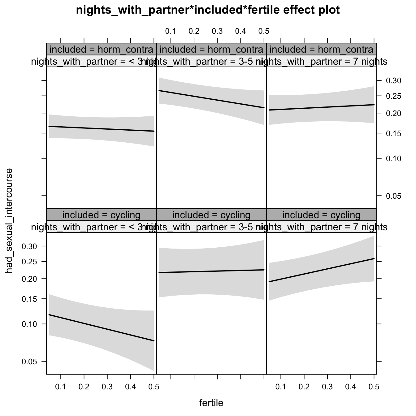
Generalized linear mixed model fit by maximum likelihood (Laplace Approximation) ['glmerMod']
Family: binomial ( probit )
Formula: had_sexual_intercourse ~ (1 | person) + nights_with_partner +
included + fertile + nights_with_partner:included + nights_with_partner:fertile +
included:fertile + nights_with_partner:included:fertile
Data: diary
AIC BIC logLik deviance df.resid
6444 6532 -3209 6418 6370
Scaled residuals:
Min 1Q Median 3Q Max
-1.488 -0.529 -0.410 -0.247 3.725
Random effects:
Groups Name Variance Std.Dev.
person (Intercept) 0.221 0.47
Number of obs: 6383, groups: person, 493
Fixed effects:
Estimate Std. Error z value Pr(>|z|)
(Intercept) -1.1637 0.1090 -10.68 <2e-16 ***
nights_with_partner3-5 nights 0.3787 0.1692 2.24 0.025 *
nights_with_partner7 nights 0.2679 0.1467 1.83 0.068 .
includedhorm_contra 0.1977 0.1252 1.58 0.114
fertile -0.5624 0.3387 -1.66 0.097 .
nights_with_partner3-5 nights:includedhorm_contra -0.0177 0.1928 -0.09 0.927
nights_with_partner7 nights:includedhorm_contra -0.1197 0.1776 -0.67 0.500
nights_with_partner3-5 nights:fertile 0.6205 0.4685 1.32 0.185
nights_with_partner7 nights:fertile 1.0606 0.4217 2.52 0.012 *
includedhorm_contra:fertile 0.4594 0.3792 1.21 0.226
nights_with_partner3-5 nights:includedhorm_contra:fertile -0.8874 0.5331 -1.66 0.096 .
nights_with_partner7 nights:includedhorm_contra:fertile -0.8432 0.4991 -1.69 0.091 .
---
Signif. codes: 0 '***' 0.001 '**' 0.01 '*' 0.05 '.' 0.1 ' ' 1
Correlation of Fixed Effects:
(Intr) ng__3-5n ng__7n incld_ fertil ng__3-5n:_ ng__7n:_ ng__3-5n: ng__7n: incl_: n__3-5n:_:
nghts__3-5n -0.639
nghts_wt_7n -0.736 0.473
inclddhrm_c -0.863 0.554 0.639
fertile -0.492 0.317 0.365 0.428
ngh__3-5n:_ 0.558 -0.877 -0.414 -0.648 -0.278
nghts__7n:_ 0.608 -0.390 -0.826 -0.704 -0.302 0.457
nght__3-5n: 0.356 -0.497 -0.264 -0.309 -0.723 0.436 0.218
nghts_w_7n: 0.394 -0.254 -0.501 -0.344 -0.803 0.223 0.414 0.581
inclddhrm_: 0.439 -0.283 -0.326 -0.499 -0.893 0.324 0.351 0.646 0.718
ng__3-5n:_: -0.311 0.436 0.232 0.354 0.635 -0.498 -0.250 -0.879 -0.510 -0.711
nght__7n:_: -0.334 0.215 0.424 0.379 0.679 -0.246 -0.506 -0.491 -0.845 -0.760 0.540
convergence code: 0
Model failed to converge with max|grad| = 0.00721173 (tol = 0.001, component 1)
H1.3. Spent night with partner
diary$spent_night_with_partner = factor(diary$spent_night_with_partner)
models$had_sexual_intercourse %>%
test_moderator("spent_night_with_partner", diary, xlevels = 2)## Warning in checkConv(attr(opt, "derivs"), opt$par, ctrl = control$checkConv, : Model failed to converge with
## max|grad| = 0.0913365 (tol = 0.001, component 1)| Df | AIC | BIC | logLik | deviance | Chisq | Chi Df | Pr(>Chisq) | |
|---|---|---|---|---|---|---|---|---|
| with_main | 7 | 5222 | 5270 | -2604 | 5208 | NA | NA | NA |
| with_mod | 9 | 5225 | 5286 | -2604 | 5207 | 1.062 | 2 | 0.5881 |
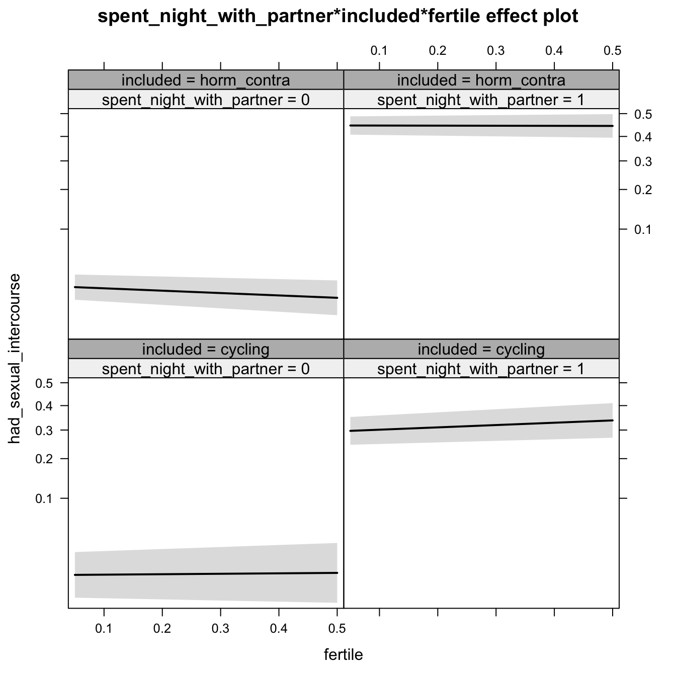
Generalized linear mixed model fit by maximum likelihood (Laplace Approximation) ['glmerMod']
Family: binomial ( probit )
Formula: had_sexual_intercourse ~ (1 | person) + spent_night_with_partner +
included + fertile + spent_night_with_partner:included +
spent_night_with_partner:fertile + included:fertile + spent_night_with_partner:included:fertile
Data: diary
AIC BIC logLik deviance df.resid
5225 5286 -2604 5207 6374
Scaled residuals:
Min 1Q Median 3Q Max
-2.199 -0.453 -0.197 -0.068 10.003
Random effects:
Groups Name Variance Std.Dev.
person (Intercept) 0.382 0.618
Number of obs: 6383, groups: person, 493
Fixed effects:
Estimate Std. Error z value Pr(>|z|)
(Intercept) -2.1339 0.1398 -15.26 <2e-16 ***
spent_night_with_partner1 1.5875 0.1462 10.86 <2e-16 ***
includedhorm_contra 0.2221 0.1554 1.43 0.15
fertile 0.0490 0.4102 0.12 0.90
spent_night_with_partner1:includedhorm_contra 0.1929 0.1653 1.17 0.24
spent_night_with_partner1:fertile 0.2085 0.4626 0.45 0.65
includedhorm_contra:fertile -0.3125 0.4700 -0.66 0.51
spent_night_with_partner1:includedhorm_contra:fertile 0.0446 0.5382 0.08 0.93
---
Signif. codes: 0 '***' 0.001 '**' 0.01 '*' 0.05 '.' 0.1 ' ' 1
Correlation of Fixed Effects:
(Intr) sp___1 incld_ fertil sp___1:_ sp___1: incl_:
spnt_ngh__1 -0.832
inclddhrm_c -0.870 0.725
fertile -0.574 0.551 0.515
spnt_n__1:_ 0.706 -0.861 -0.808 -0.487
spnt_ng__1: 0.503 -0.607 -0.453 -0.891 0.537
inclddhrm_: 0.502 -0.482 -0.580 -0.873 0.548 0.777
spnt___1:_: -0.435 0.524 0.503 0.765 -0.616 -0.859 -0.878
convergence code: 0
Model failed to converge with max|grad| = 0.0913365 (tol = 0.001, component 1)
H1.3. Partner initiated sex
models$partner_initiated_sexual_intercourse = glmer(partner_initiated_sexual_intercourse ~ included * fertile + ( 1 | person), data = diary, family = binomial(link = "probit"))
do_model(models$partner_initiated_sexual_intercourse, diary)Narrow window
model %>%
print_summary() %>%
plot_all_effects()Generalized linear mixed model fit by maximum likelihood (Laplace Approximation) ['glmerMod']
Family: binomial ( probit )
Formula: partner_initiated_sexual_intercourse ~ included * fertile + (1 | person)
Data: diary
AIC BIC logLik deviance df.resid
1862 1888 -926 1852 1398
Scaled residuals:
Min 1Q Median 3Q Max
-1.455 -1.214 0.712 0.758 0.953
Random effects:
Groups Name Variance Std.Dev.
person (Intercept) 0.0423 0.206
Number of obs: 1403, groups: person, 401
Fixed effects:
Estimate Std. Error z value Pr(>|z|)
(Intercept) 0.2603 0.0926 2.81 0.0049 **
includedhorm_contra 0.1178 0.1081 1.09 0.2761
fertile -0.1440 0.3095 -0.47 0.6418
includedhorm_contra:fertile 0.1054 0.3689 0.29 0.7750
---
Signif. codes: 0 '***' 0.001 '**' 0.01 '*' 0.05 '.' 0.1 ' ' 1
Correlation of Fixed Effects:
(Intr) incld_ fertil
inclddhrm_c -0.847
fertile -0.657 0.561
inclddhrm_: 0.555 -0.655 -0.839
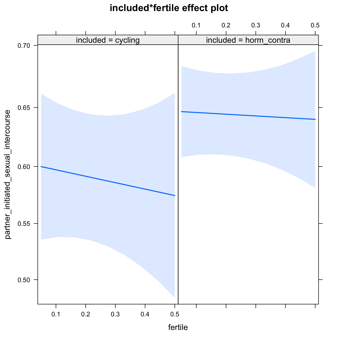
Diagnostics
model %>%
plot_outcome(diary) %>%
print_diagnostics()
## Error in qqnorm.default(resid(obj)): y is empty or has only NAs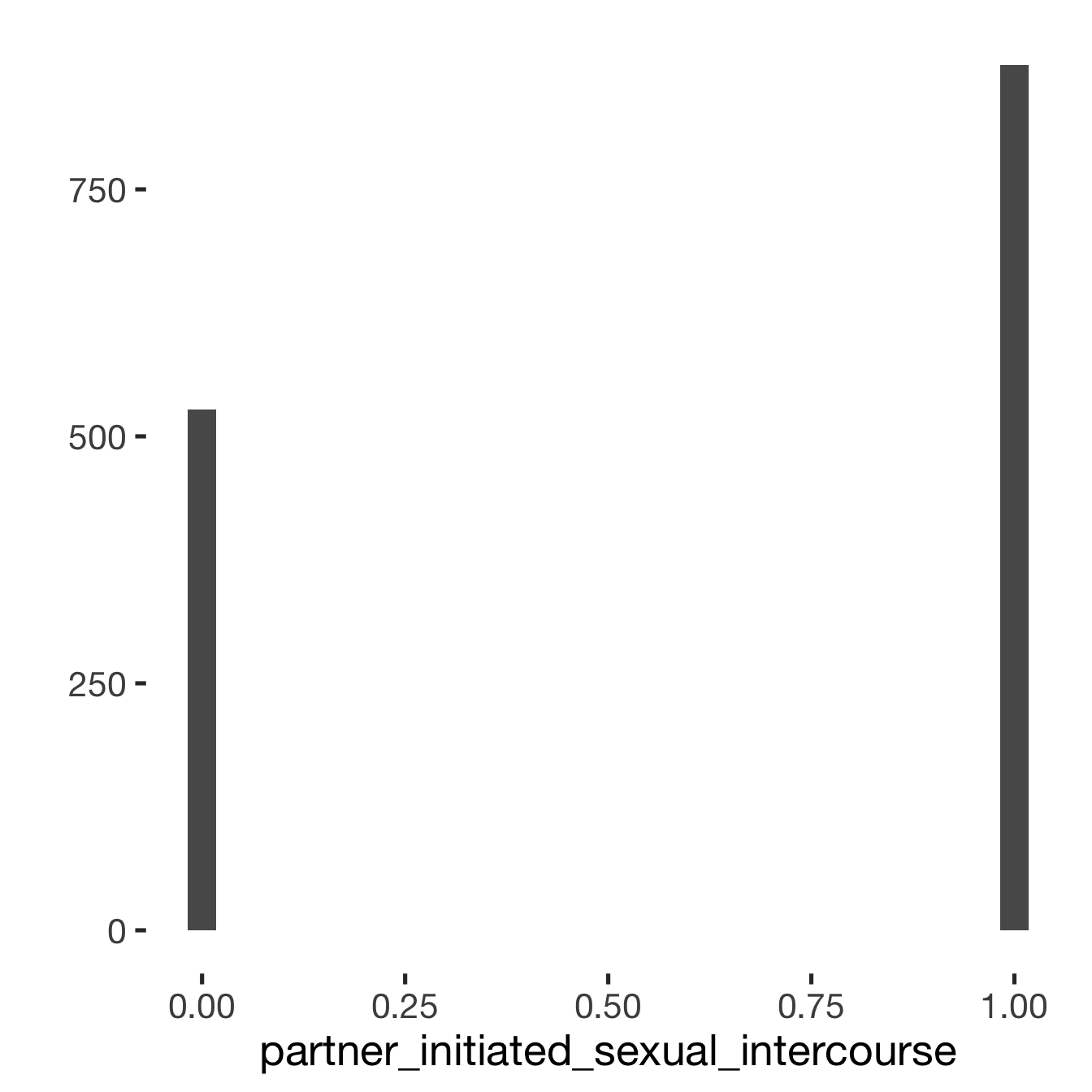
Adjusting for self esteem
model %>%
adjust_for_self_esteem(diary)##
##
## ```
## Linear mixed model fit by REML. t-tests use Satterthwaite's method ['lmerModLmerTest']
## Formula: form
## Data: diary
##
## REML criterion at convergence: 1959
##
## Scaled residuals:
## Min 1Q Median 3Q Max
## -1.565 -1.216 0.676 0.780 1.080
##
## Random effects:
## Groups Name Variance Std.Dev.
## person (Intercept) 0.0076 0.0872
## Residual 0.2265 0.4759
## Number of obs: 1401, groups: person, 401
##
## Fixed effects:
## Estimate Std. Error df t value Pr(>|t|)
## (Intercept) 0.7219 0.0631 723.1879 11.43 <2e-16 ***
## includedhorm_contra 0.0471 0.0405 605.4745 1.16 0.25
## fertile -0.0394 0.1156 1359.6970 -0.34 0.73
## self_esteem_1 -0.0277 0.0119 847.7566 -2.32 0.02 *
## includedhorm_contra:fertile 0.0149 0.1373 1369.3125 0.11 0.91
## ---
## Signif. codes: 0 '***' 0.001 '**' 0.01 '*' 0.05 '.' 0.1 ' ' 1
##
## Correlation of Fixed Effects:
## (Intr) incld_ fertil slf__1
## inclddhrm_c -0.451
## fertile -0.317 0.559
## self_estm_1 -0.837 -0.021 -0.048
## inclddhrm_: 0.243 -0.650 -0.843 0.069
##
## ```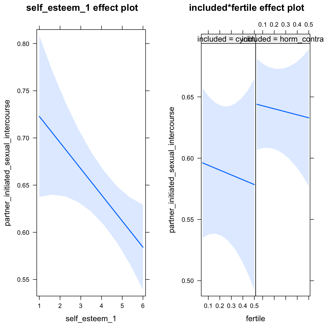
Broad window
outcome = names(model@frame)[1]
broad_models[[outcome]] <<- model %>%
switch_window_to_broad(diary)Generalized linear mixed model fit by maximum likelihood (Laplace Approximation) ['glmerMod']
Family: binomial ( probit )
Formula: partner_initiated_sexual_intercourse ~ included * fertile + (1 | person)
Data: diary2
AIC BIC logLik deviance df.resid
2261 2288 -1126 2251 1691
Scaled residuals:
Min 1Q Median 3Q Max
-1.539 -1.173 0.699 0.774 0.992
Random effects:
Groups Name Variance Std.Dev.
person (Intercept) 0.0625 0.25
Number of obs: 1696, groups: person, 411
Fixed effects:
Estimate Std. Error z value Pr(>|z|)
(Intercept) 0.2619 0.0959 2.73 0.0063 **
includedhorm_contra 0.1333 0.1121 1.19 0.2345
fertile -0.0573 0.3159 -0.18 0.8560
includedhorm_contra:fertile -0.2100 0.3730 -0.56 0.5734
---
Signif. codes: 0 '***' 0.001 '**' 0.01 '*' 0.05 '.' 0.1 ' ' 1
Correlation of Fixed Effects:
(Intr) incld_ fertil
inclddhrm_c -0.849
fertile -0.716 0.613
inclddhrm_: 0.608 -0.720 -0.847
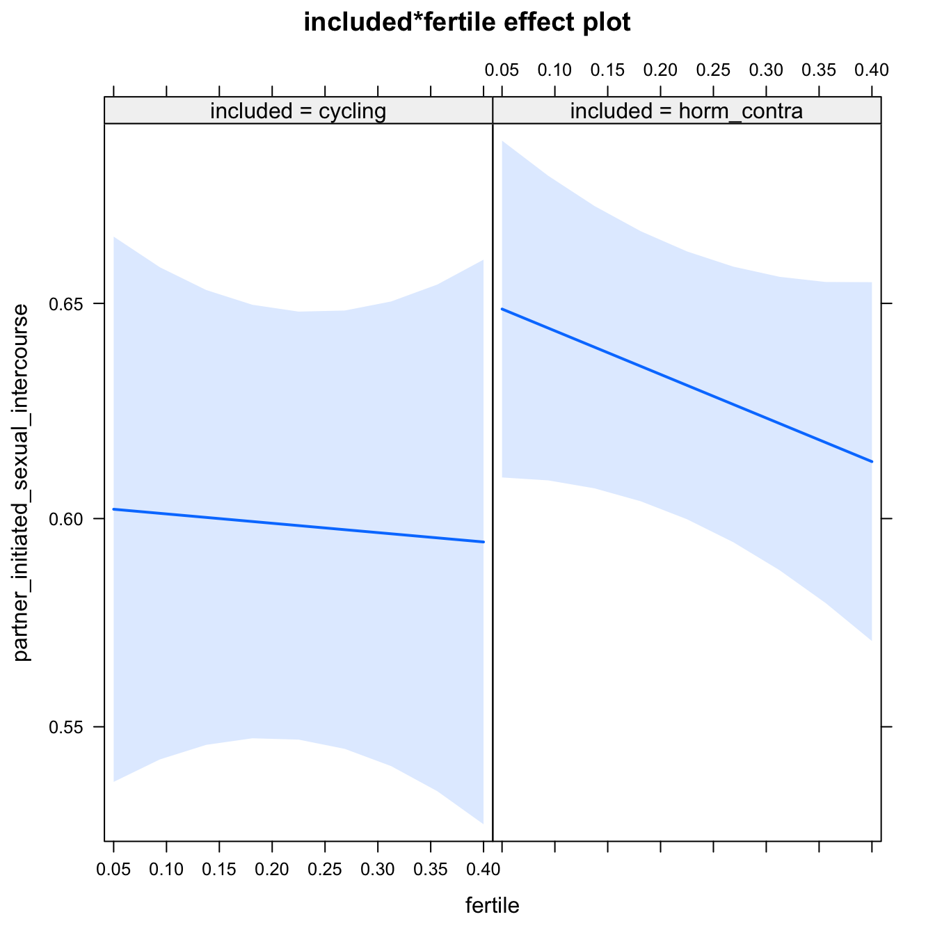
Diagnostics
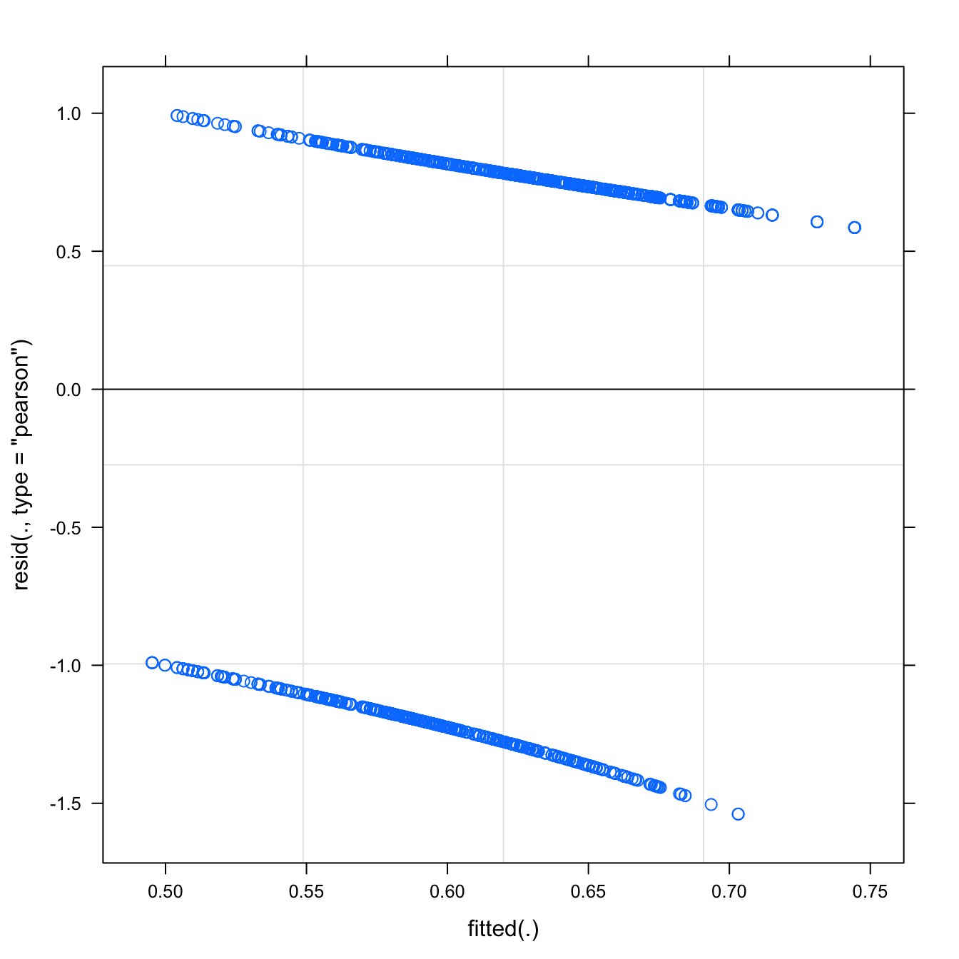
## Warning: 'sjp.lmer' is deprecated.
## Use 'plot_model' instead.
## See help("Deprecated")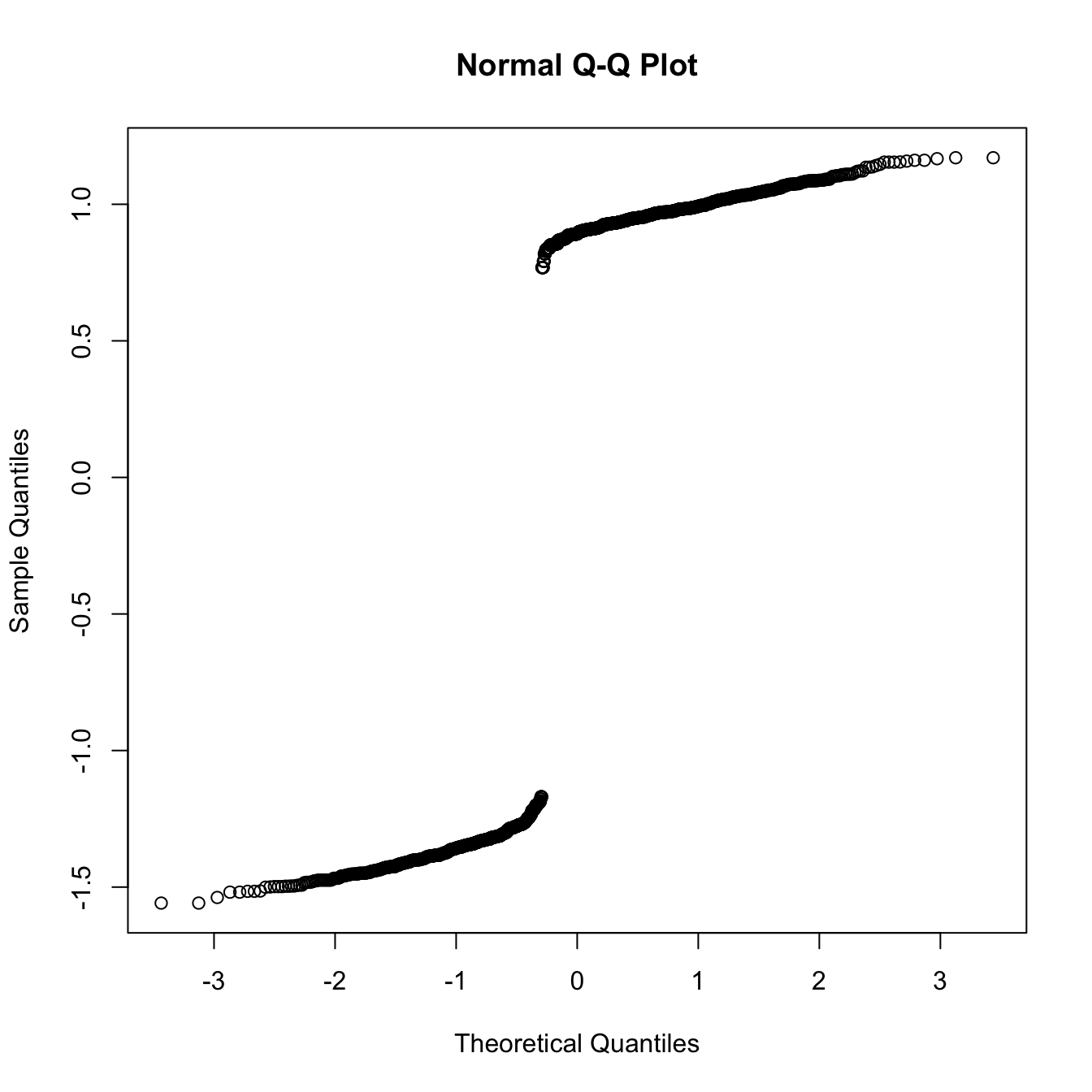
## Warning: 'sjp.lmer' is deprecated.
## Use 'plot_model' instead.
## See help("Deprecated")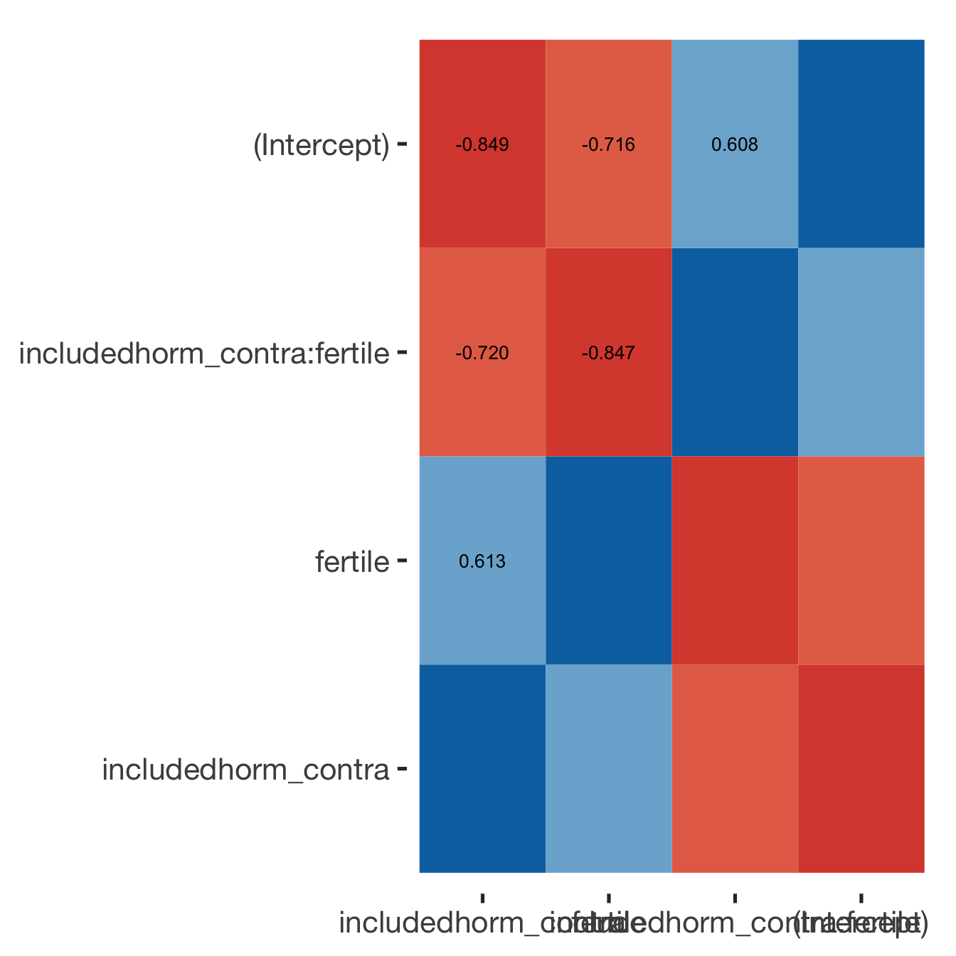
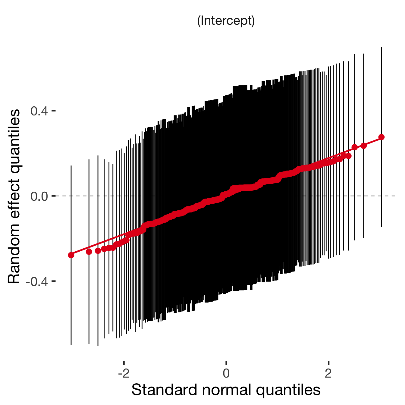
Adjusting for self esteem
broad_models[[outcome]] %>%
adjust_for_self_esteem(diary2)##
##
## ```
## Linear mixed model fit by REML. t-tests use Satterthwaite's method ['lmerModLmerTest']
## Formula: form
## Data: diary
##
## REML criterion at convergence: 2377
##
## Scaled residuals:
## Min 1Q Median 3Q Max
## -1.562 -1.180 0.665 0.794 1.119
##
## Random effects:
## Groups Name Variance Std.Dev.
## person (Intercept) 0.0104 0.102
## Residual 0.2260 0.475
## Number of obs: 1694, groups: person, 411
##
## Fixed effects:
## Estimate Std. Error df t value Pr(>|t|)
## (Intercept) 0.71409 0.06037 935.28289 11.83 <2e-16 ***
## includedhorm_contra 0.05177 0.04166 839.17963 1.24 0.214
## fertile -0.00712 0.11704 1669.81306 -0.06 0.951
## self_esteem_1 -0.02607 0.01099 1079.22430 -2.37 0.018 *
## includedhorm_contra:fertile -0.09687 0.13795 1674.62182 -0.70 0.483
## ---
## Signif. codes: 0 '***' 0.001 '**' 0.01 '*' 0.05 '.' 0.1 ' ' 1
##
## Correlation of Fixed Effects:
## (Intr) incld_ fertil slf__1
## inclddhrm_c -0.493
## fertile -0.391 0.611
## self_estm_1 -0.807 -0.014 -0.038
## inclddhrm_: 0.320 -0.713 -0.849 0.047
##
## ```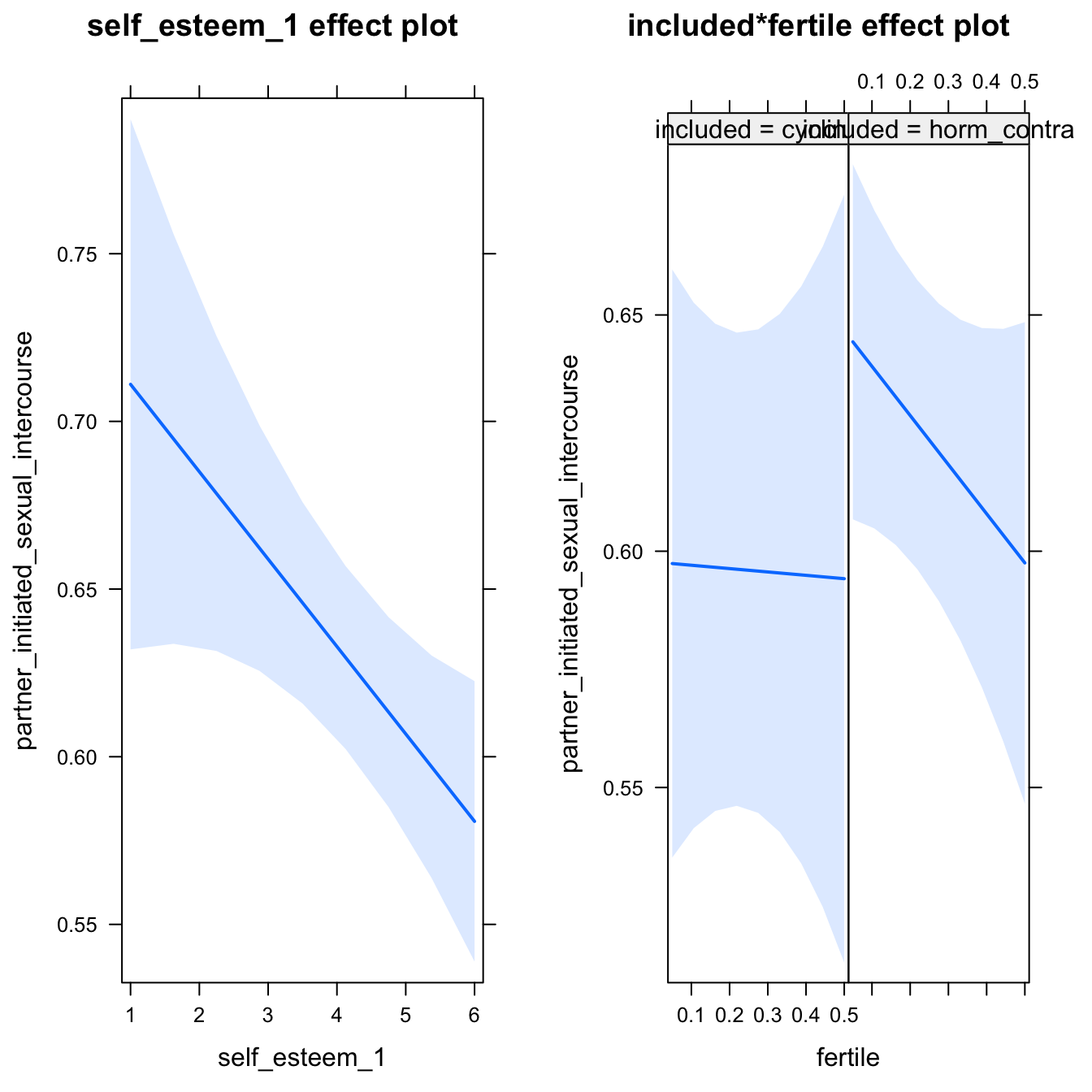
bla = 2H1.4. Self-reported perceived desirability
models$desirability_1 = lmer(desirability_1 ~ included * fertile + ( 1 | person), data = diary)
do_model(models$desirability_1, diary)Narrow window
model %>%
print_summary() %>%
plot_all_effects()Linear mixed model fit by REML. t-tests use Satterthwaite's method ['lmerModLmerTest']
Formula: desirability_1 ~ included * fertile + (1 | person)
Data: diary
REML criterion at convergence: 20748
Scaled residuals:
Min 1Q Median 3Q Max
-3.299 -0.613 0.043 0.662 3.206
Random effects:
Groups Name Variance Std.Dev.
person (Intercept) 0.675 0.822
Residual 1.295 1.138
Number of obs: 6379, groups: person, 493
Fixed effects:
Estimate Std. Error df t value Pr(>|t|)
(Intercept) 3.7223 0.0784 586.8256 47.48 <2e-16 ***
includedhorm_contra -0.0661 0.0930 592.1023 -0.71 0.477
fertile 0.3661 0.1272 5978.7195 2.88 0.004 **
includedhorm_contra:fertile -0.3840 0.1523 5985.3829 -2.52 0.012 *
---
Signif. codes: 0 '***' 0.001 '**' 0.01 '*' 0.05 '.' 0.1 ' ' 1
Correlation of Fixed Effects:
(Intr) incld_ fertil
inclddhrm_c -0.843
fertile -0.306 0.258
inclddhrm_: 0.255 -0.309 -0.835
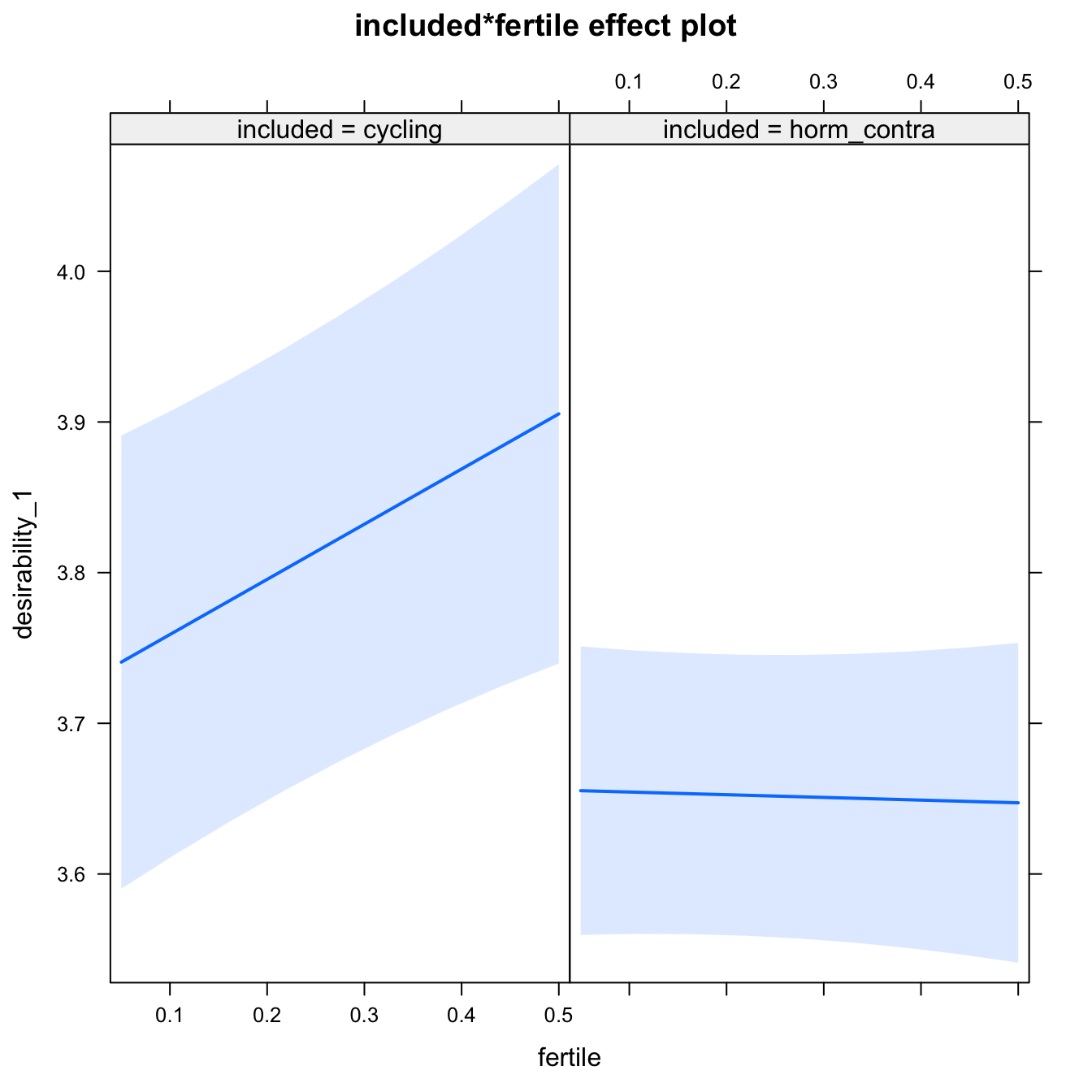
Diagnostics
model %>%
plot_outcome(diary) %>%
print_diagnostics()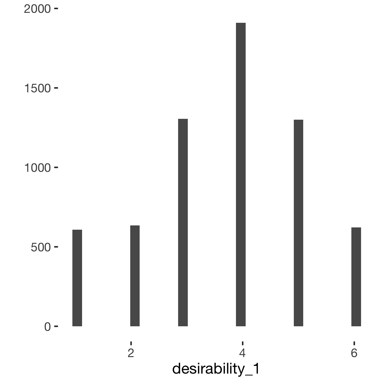
## Error in qqnorm.default(resid(obj)): y is empty or has only NAs
Adjusting for self esteem
model %>%
adjust_for_self_esteem(diary)##
##
## ```
## Linear mixed model fit by REML. t-tests use Satterthwaite's method ['lmerModLmerTest']
## Formula: form
## Data: diary
##
## REML criterion at convergence: 19267
##
## Scaled residuals:
## Min 1Q Median 3Q Max
## -3.958 -0.595 0.040 0.615 4.565
##
## Random effects:
## Groups Name Variance Std.Dev.
## person (Intercept) 0.401 0.634
## Residual 1.046 1.023
## Number of obs: 6379, groups: person, 493
##
## Fixed effects:
## Estimate Std. Error df t value Pr(>|t|)
## (Intercept) 1.1927 0.0878 1706.6927 13.58 <2e-16 ***
## includedhorm_contra -0.0129 0.0744 622.5363 -0.17 0.8626
## fertile 0.3486 0.1142 5999.9696 3.05 0.0023 **
## self_esteem_1 0.5889 0.0143 6123.8023 41.17 <2e-16 ***
## includedhorm_contra:fertile -0.4088 0.1367 6008.4391 -2.99 0.0028 **
## ---
## Signif. codes: 0 '***' 0.001 '**' 0.01 '*' 0.05 '.' 0.1 ' ' 1
##
## Correlation of Fixed Effects:
## (Intr) incld_ fertil slf__1
## inclddhrm_c -0.614
## fertile -0.243 0.289
## self_estm_1 -0.700 0.018 -0.003
## inclddhrm_: 0.208 -0.346 -0.835 -0.005
##
## ```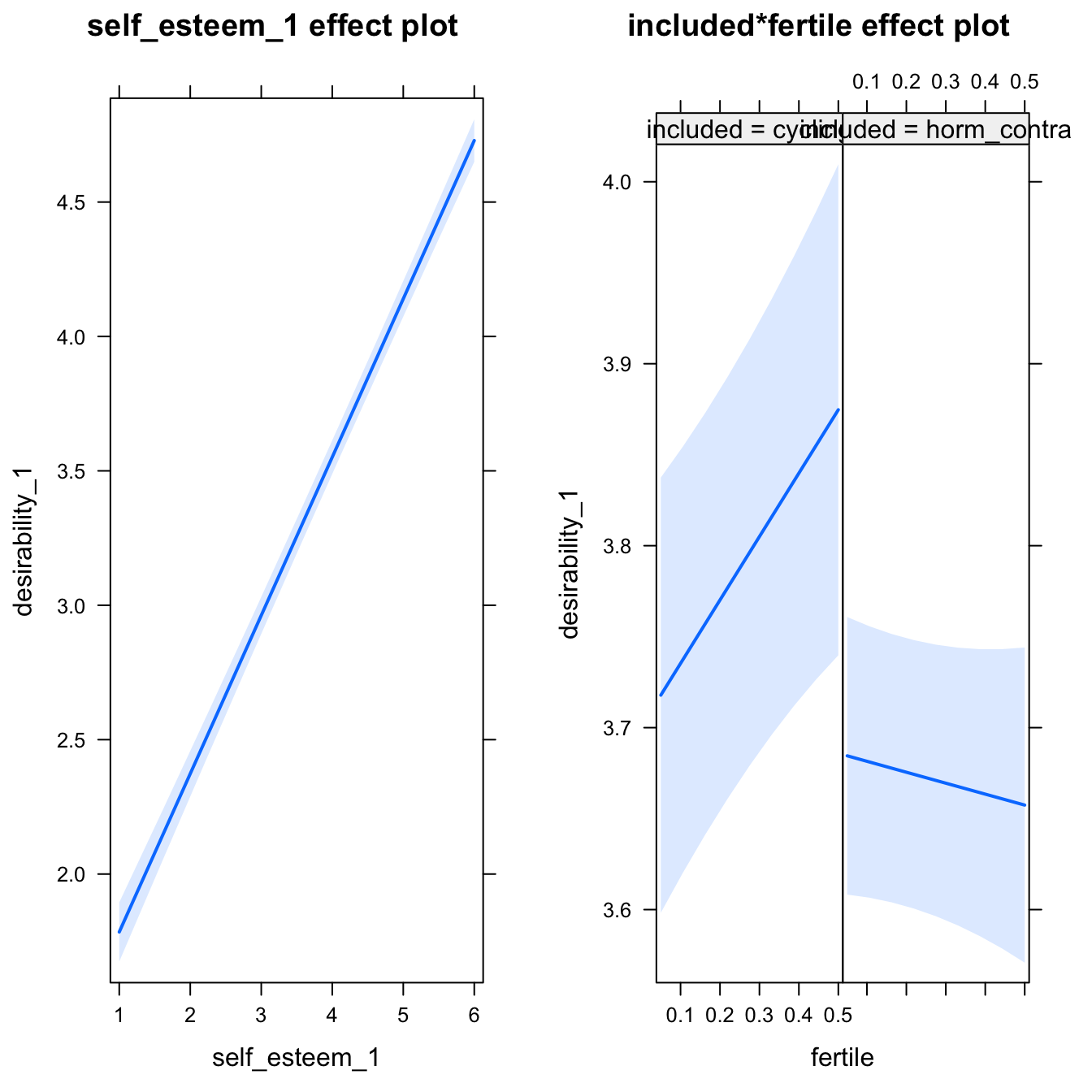
Broad window
outcome = names(model@frame)[1]
broad_models[[outcome]] <<- model %>%
switch_window_to_broad(diary)Linear mixed model fit by REML. t-tests use Satterthwaite's method ['lmerModLmerTest']
Formula: form
Data: diary2
REML criterion at convergence: 24997
Scaled residuals:
Min 1Q Median 3Q Max
-3.267 -0.622 0.030 0.653 3.328
Random effects:
Groups Name Variance Std.Dev.
person (Intercept) 0.674 0.821
Residual 1.287 1.134
Number of obs: 7741, groups: person, 493
Fixed effects:
Estimate Std. Error df t value Pr(>|t|)
(Intercept) 3.7254 0.0784 621.2148 47.49 <2e-16 ***
includedhorm_contra -0.0690 0.0930 626.8709 -0.74 0.4585
fertile 0.3837 0.1271 7363.0957 3.02 0.0026 **
includedhorm_contra:fertile -0.3821 0.1518 7371.5023 -2.52 0.0119 *
---
Signif. codes: 0 '***' 0.001 '**' 0.01 '*' 0.05 '.' 0.1 ' ' 1
Correlation of Fixed Effects:
(Intr) incld_ fertil
inclddhrm_c -0.843
fertile -0.340 0.287
inclddhrm_: 0.285 -0.344 -0.837
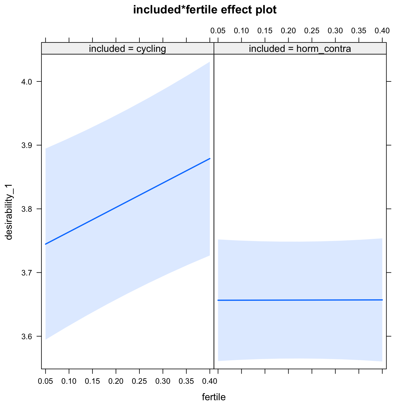
Diagnostics
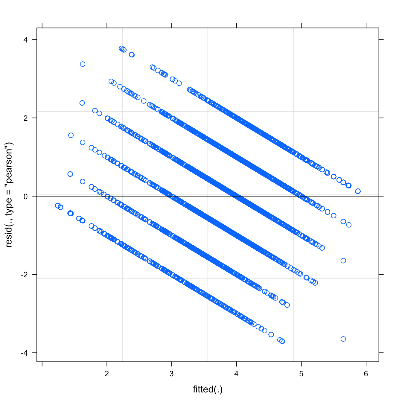
## Warning: 'sjp.lmer' is deprecated.
## Use 'plot_model' instead.
## See help("Deprecated")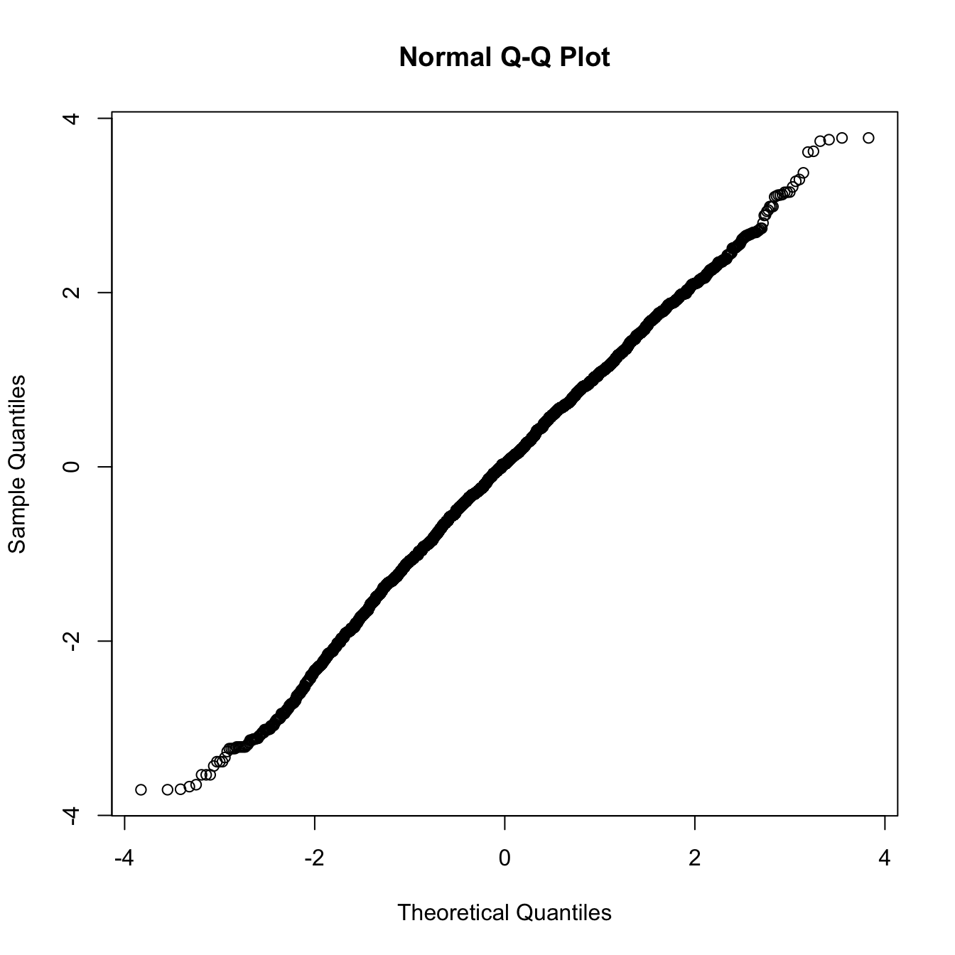
## Warning: 'sjp.lmer' is deprecated.
## Use 'plot_model' instead.
## See help("Deprecated")
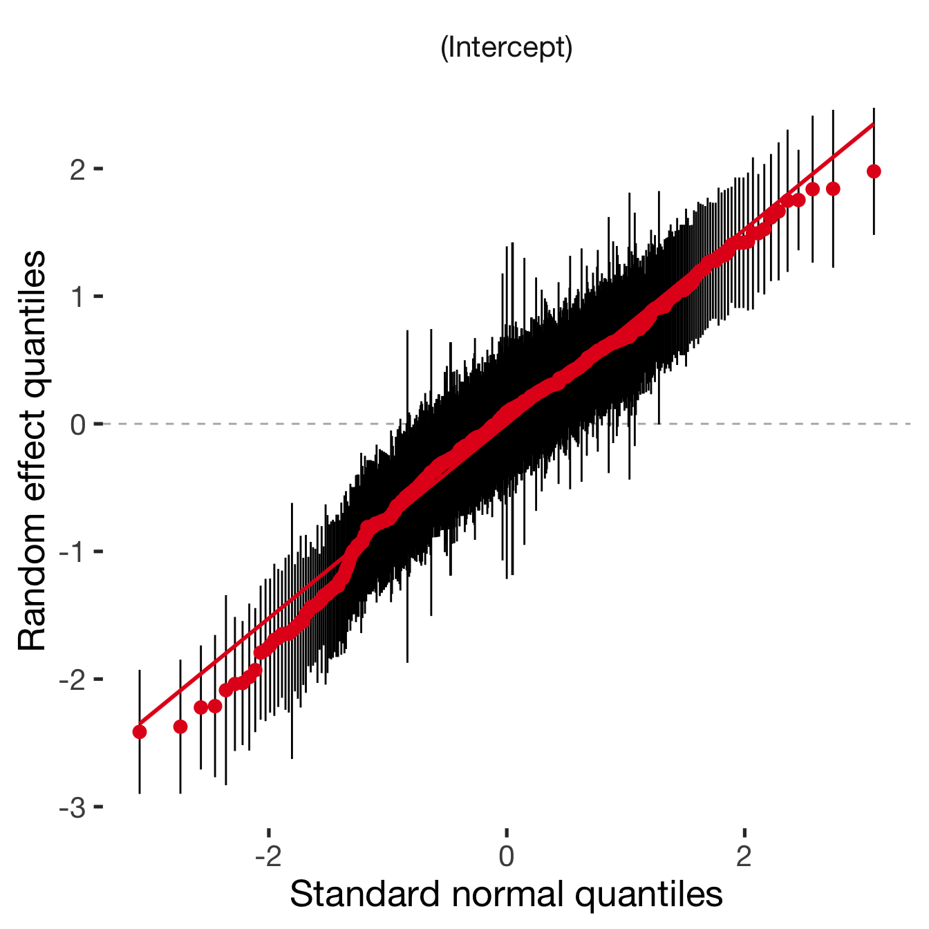
Adjusting for self esteem
broad_models[[outcome]] %>%
adjust_for_self_esteem(diary2)##
##
## ```
## Linear mixed model fit by REML. t-tests use Satterthwaite's method ['lmerModLmerTest']
## Formula: form
## Data: diary
##
## REML criterion at convergence: 23245
##
## Scaled residuals:
## Min 1Q Median 3Q Max
## -3.951 -0.600 0.029 0.623 4.573
##
## Random effects:
## Groups Name Variance Std.Dev.
## person (Intercept) 0.392 0.626
## Residual 1.044 1.022
## Number of obs: 7741, groups: person, 493
##
## Fixed effects:
## Estimate Std. Error df t value Pr(>|t|)
## (Intercept) 1.2306 0.0837 1692.6074 14.71 <2e-16 ***
## includedhorm_contra -0.0179 0.0740 673.1576 -0.24 0.8091
## fertile 0.3358 0.1144 7391.2650 2.94 0.0033 **
## self_esteem_1 0.5807 0.0130 7468.8888 44.73 <2e-16 ***
## includedhorm_contra:fertile -0.3941 0.1366 7401.5860 -2.89 0.0039 **
## ---
## Signif. codes: 0 '***' 0.001 '**' 0.01 '*' 0.05 '.' 0.1 ' ' 1
##
## Correlation of Fixed Effects:
## (Intr) incld_ fertil slf__1
## inclddhrm_c -0.638
## fertile -0.282 0.325
## self_estm_1 -0.667 0.016 -0.009
## inclddhrm_: 0.242 -0.390 -0.837 -0.002
##
## ```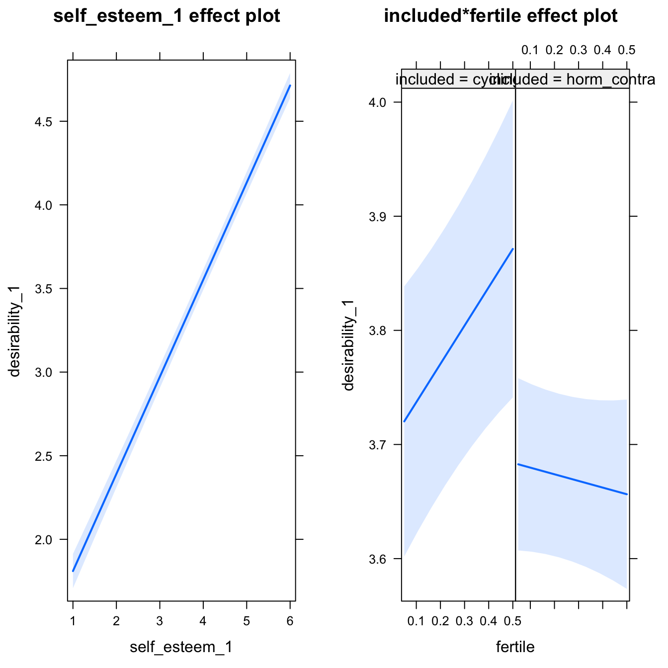
bla = 2Moderators
H4.4. Neuroticism
models$desirability_1 %>%
test_moderator("BFI_neuro", diary)| Df | AIC | BIC | logLik | deviance | Chisq | Chi Df | Pr(>Chisq) | |
|---|---|---|---|---|---|---|---|---|
| with_main | 8 | 20693 | 20747 | -10338 | 20677 | NA | NA | NA |
| with_mod | 10 | 20684 | 20752 | -10332 | 20664 | 12.4 | 2 | 0.00203 |
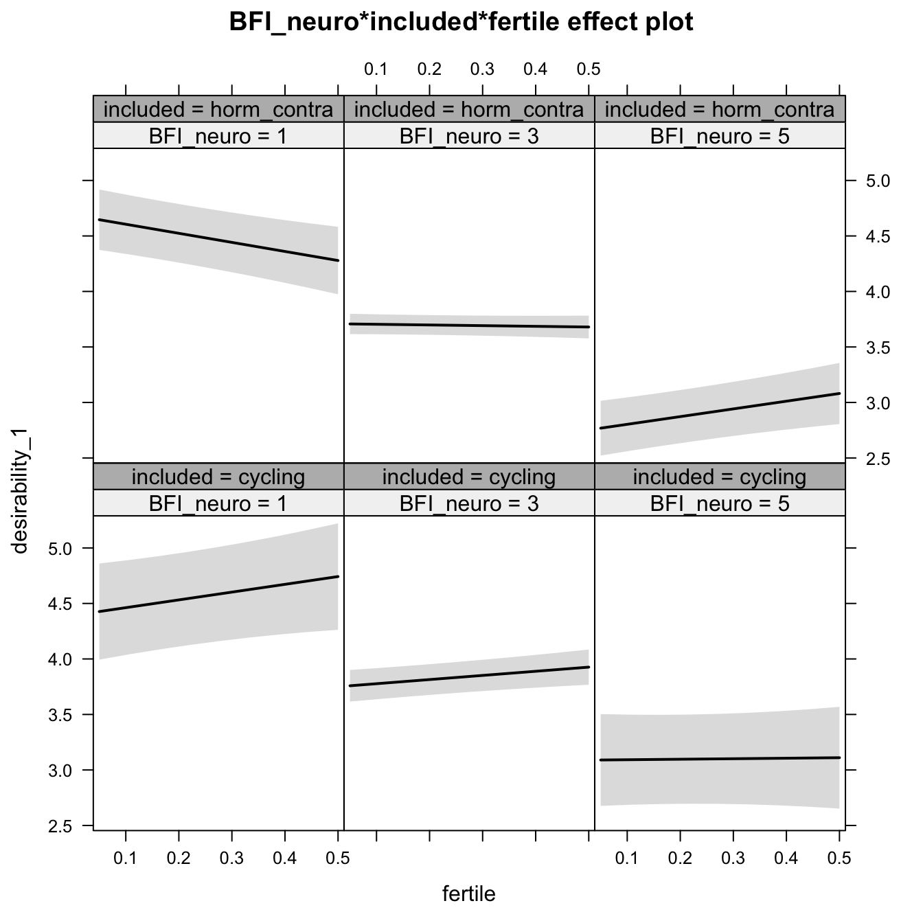
Linear mixed model fit by REML. t-tests use Satterthwaite's method ['lmerModLmerTest']
Formula: desirability_1 ~ (1 | person) + BFI_neuro + included + fertile +
BFI_neuro:included + BFI_neuro:fertile + included:fertile + BFI_neuro:included:fertile
Data: diary
REML criterion at convergence: 20688
Scaled residuals:
Min 1Q Median 3Q Max
-3.310 -0.605 0.026 0.666 3.272
Random effects:
Groups Name Variance Std.Dev.
person (Intercept) 0.588 0.767
Residual 1.294 1.137
Number of obs: 6379, groups: person, 493
Fixed effects:
Estimate Std. Error df t value Pr(>|t|)
(Intercept) 4.718 0.327 603.551 14.44 <2e-16 ***
BFI_neuro -0.326 0.104 604.846 -3.13 0.0018 **
includedhorm_contra 0.457 0.385 608.093 1.19 0.2352
fertile 0.864 0.555 5987.901 1.56 0.1196
BFI_neuro:includedhorm_contra -0.162 0.122 609.297 -1.33 0.1845
BFI_neuro:fertile -0.164 0.177 5971.508 -0.92 0.3552
includedhorm_contra:fertile -2.059 0.660 5990.266 -3.12 0.0018 **
BFI_neuro:includedhorm_contra:fertile 0.542 0.209 5976.905 2.59 0.0096 **
---
Signif. codes: 0 '***' 0.001 '**' 0.01 '*' 0.05 '.' 0.1 ' ' 1
Correlation of Fixed Effects:
(Intr) BFI_nr incld_ fertil BFI_n:_ BFI_n: incl_:
BFI_neuro -0.974
inclddhrm_c -0.849 0.827
fertile -0.327 0.318 0.277
BFI_nr:ncl_ 0.831 -0.853 -0.973 -0.271
BFI_nr:frtl 0.318 -0.326 -0.270 -0.973 0.279
inclddhrm_: 0.275 -0.268 -0.328 -0.841 0.319 0.819
BFI_nr:nc_: -0.269 0.276 0.320 0.824 -0.328 -0.847 -0.973
H1.5. Sexy clothes
models$sexy_clothes = lmer(sexy_clothes ~ included * fertile + ( 1 | person), data = diary)
do_model(models$sexy_clothes, diary)Narrow window
model %>%
print_summary() %>%
plot_all_effects()Linear mixed model fit by REML. t-tests use Satterthwaite's method ['lmerModLmerTest']
Formula: sexy_clothes ~ included * fertile + (1 | person)
Data: diary
REML criterion at convergence: 18258
Scaled residuals:
Min 1Q Median 3Q Max
-4.200 -0.617 -0.008 0.624 3.855
Random effects:
Groups Name Variance Std.Dev.
person (Intercept) 0.556 0.746
Residual 0.864 0.930
Number of obs: 6380, groups: person, 493
Fixed effects:
Estimate Std. Error df t value Pr(>|t|)
(Intercept) 3.1616 0.0697 571.7007 45.37 <2e-16 ***
includedhorm_contra 0.0176 0.0826 575.9672 0.21 0.83
fertile -0.1430 0.1040 5967.0290 -1.38 0.17
includedhorm_contra:fertile 0.0856 0.1245 5972.5882 0.69 0.49
---
Signif. codes: 0 '***' 0.001 '**' 0.01 '*' 0.05 '.' 0.1 ' ' 1
Correlation of Fixed Effects:
(Intr) incld_ fertil
inclddhrm_c -0.844
fertile -0.281 0.237
inclddhrm_: 0.235 -0.284 -0.835
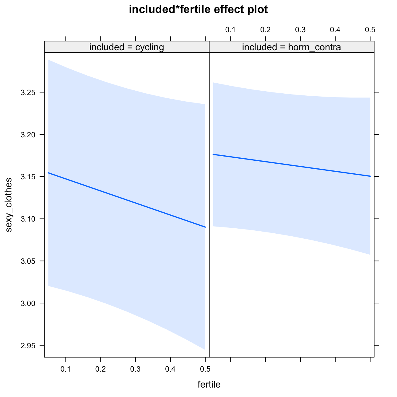
Diagnostics
model %>%
plot_outcome(diary) %>%
print_diagnostics()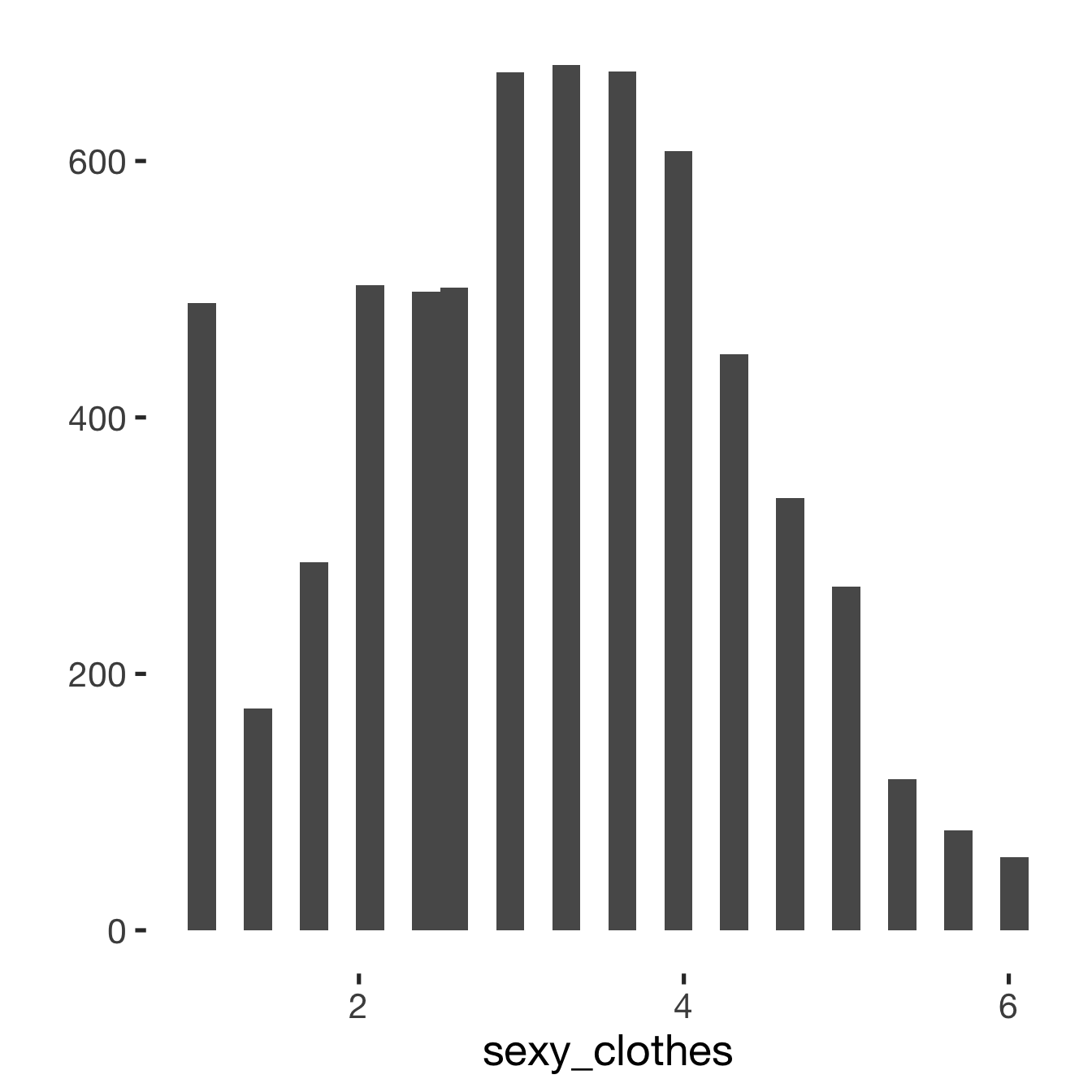
## Error in qqnorm.default(resid(obj)): y is empty or has only NAs
Adjusting for self esteem
model %>%
adjust_for_self_esteem(diary)##
##
## ```
## Linear mixed model fit by REML. t-tests use Satterthwaite's method ['lmerModLmerTest']
## Formula: form
## Data: diary
##
## REML criterion at convergence: 18020
##
## Scaled residuals:
## Min 1Q Median 3Q Max
## -3.986 -0.618 -0.009 0.624 3.968
##
## Random effects:
## Groups Name Variance Std.Dev.
## person (Intercept) 0.533 0.730
## Residual 0.832 0.912
## Number of obs: 6379, groups: person, 493
##
## Fixed effects:
## Estimate Std. Error df t value Pr(>|t|)
## (Intercept) 2.2780 0.0883 1363.5326 25.79 <2e-16 ***
## includedhorm_contra 0.0363 0.0809 575.2365 0.45 0.65
## fertile -0.1487 0.1020 5964.5499 -1.46 0.15
## self_esteem_1 0.2057 0.0131 6362.3111 15.75 <2e-16 ***
## includedhorm_contra:fertile 0.0759 0.1222 5970.1133 0.62 0.53
## ---
## Signif. codes: 0 '***' 0.001 '**' 0.01 '*' 0.05 '.' 0.1 ' ' 1
##
## Correlation of Fixed Effects:
## (Intr) incld_ fertil slf__1
## inclddhrm_c -0.661
## fertile -0.215 0.237
## self_estm_1 -0.635 0.015 -0.004
## inclddhrm_: 0.185 -0.284 -0.835 -0.005
##
## ```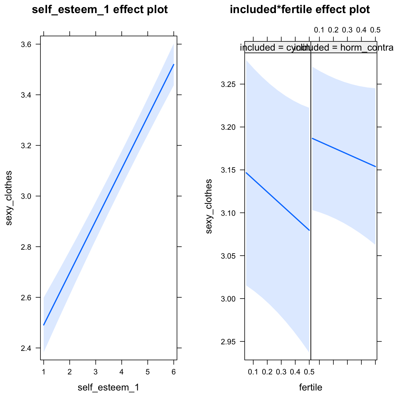
Broad window
outcome = names(model@frame)[1]
broad_models[[outcome]] <<- model %>%
switch_window_to_broad(diary)Linear mixed model fit by REML. t-tests use Satterthwaite's method ['lmerModLmerTest']
Formula: form
Data: diary2
REML criterion at convergence: 22084
Scaled residuals:
Min 1Q Median 3Q Max
-4.114 -0.616 -0.009 0.618 3.931
Random effects:
Groups Name Variance Std.Dev.
person (Intercept) 0.547 0.740
Residual 0.874 0.935
Number of obs: 7742, groups: person, 493
Fixed effects:
Estimate Std. Error df t value Pr(>|t|)
(Intercept) 3.1587 0.0694 600.1756 45.50 <2e-16 ***
includedhorm_contra 0.0194 0.0823 604.8485 0.24 0.81
fertile -0.1510 0.1048 7349.0060 -1.44 0.15
includedhorm_contra:fertile 0.0974 0.1252 7356.4344 0.78 0.44
---
Signif. codes: 0 '***' 0.001 '**' 0.01 '*' 0.05 '.' 0.1 ' ' 1
Correlation of Fixed Effects:
(Intr) incld_ fertil
inclddhrm_c -0.843
fertile -0.317 0.267
inclddhrm_: 0.265 -0.321 -0.837
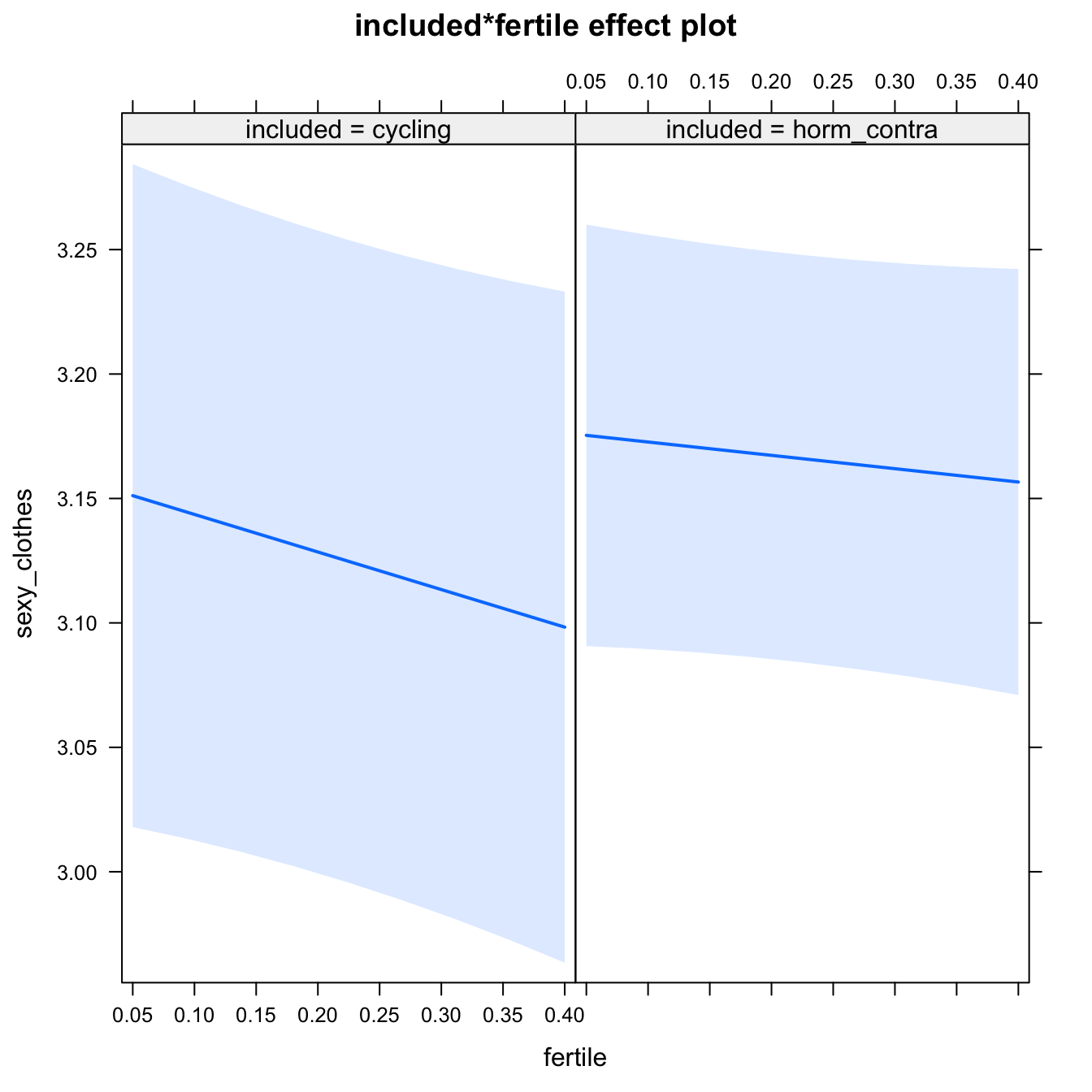
Diagnostics
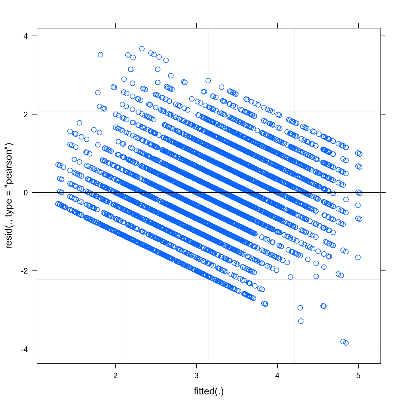
## Warning: 'sjp.lmer' is deprecated.
## Use 'plot_model' instead.
## See help("Deprecated")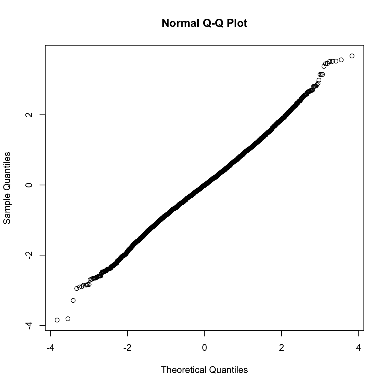
## Warning: 'sjp.lmer' is deprecated.
## Use 'plot_model' instead.
## See help("Deprecated")
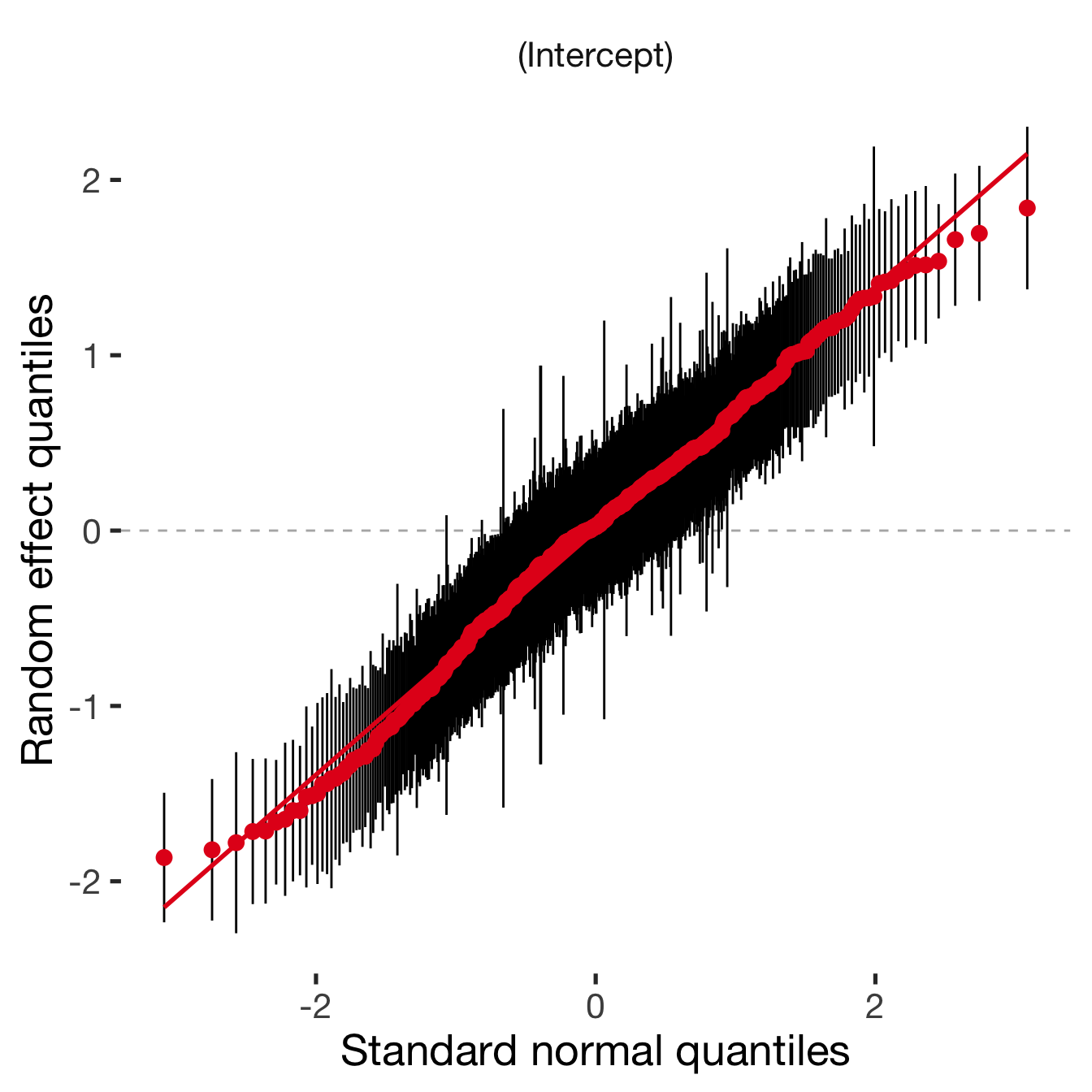
Adjusting for self esteem
broad_models[[outcome]] %>%
adjust_for_self_esteem(diary2)##
##
## ```
## Linear mixed model fit by REML. t-tests use Satterthwaite's method ['lmerModLmerTest']
## Formula: form
## Data: diary
##
## REML criterion at convergence: 21770
##
## Scaled residuals:
## Min 1Q Median 3Q Max
## -3.892 -0.618 -0.006 0.622 3.968
##
## Random effects:
## Groups Name Variance Std.Dev.
## person (Intercept) 0.516 0.718
## Residual 0.840 0.916
## Number of obs: 7741, groups: person, 493
##
## Fixed effects:
## Estimate Std. Error df t value Pr(>|t|)
## (Intercept) 2.2391 0.0846 1318.0402 26.46 <2e-16 ***
## includedhorm_contra 0.0383 0.0801 606.0143 0.48 0.63
## fertile -0.1683 0.1028 7348.0511 -1.64 0.10
## self_esteem_1 0.2141 0.0119 7722.0236 18.03 <2e-16 ***
## includedhorm_contra:fertile 0.0923 0.1227 7355.3598 0.75 0.45
## ---
## Signif. codes: 0 '***' 0.001 '**' 0.01 '*' 0.05 '.' 0.1 ' ' 1
##
## Correlation of Fixed Effects:
## (Intr) incld_ fertil slf__1
## inclddhrm_c -0.681
## fertile -0.249 0.269
## self_estm_1 -0.603 0.013 -0.009
## inclddhrm_: 0.215 -0.323 -0.837 -0.002
##
## ```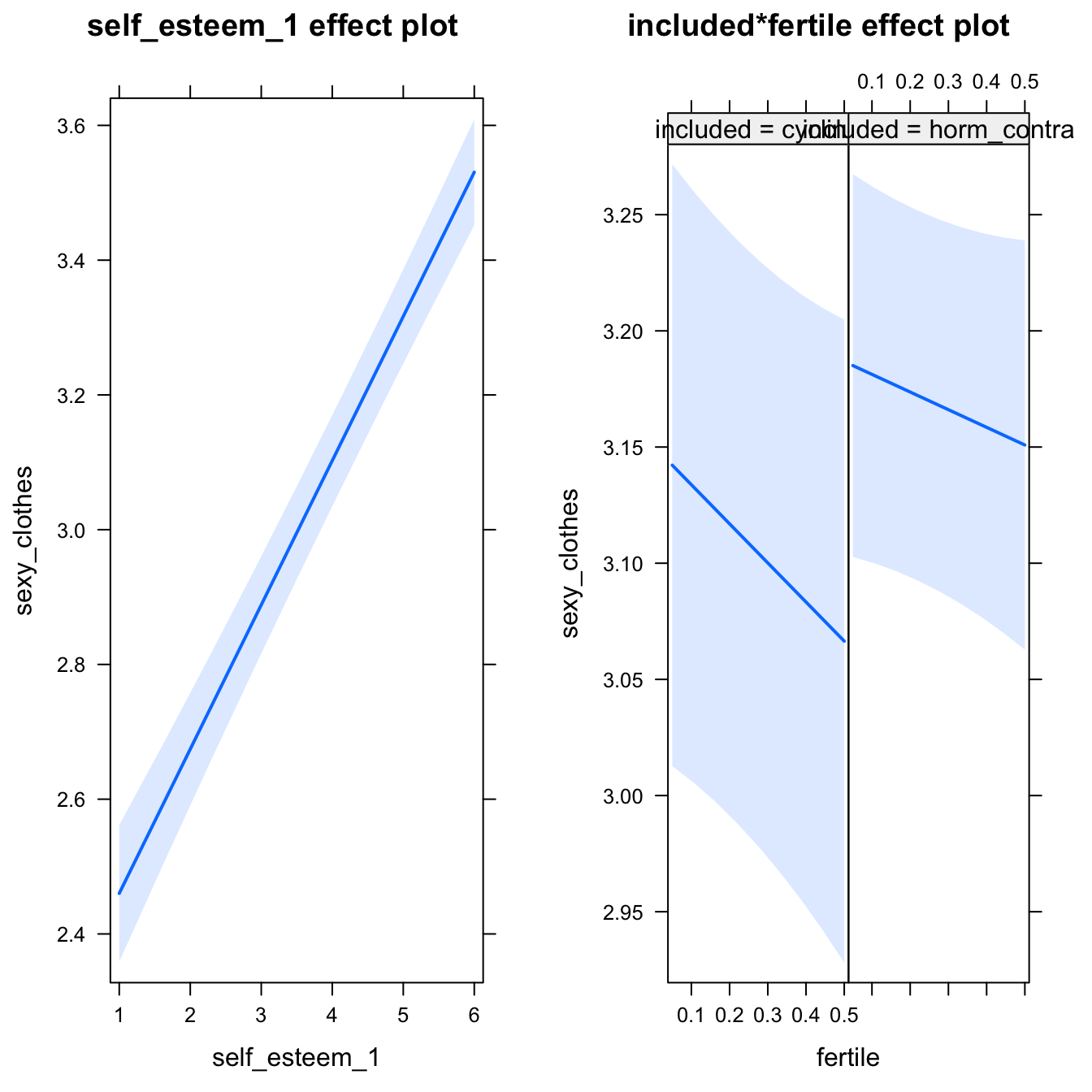
bla = 2H1.6. Male mate retention
models$partner_mate_retention = lmer(partner_mate_retention ~ included * fertile + ( 1 | person), data = diary)
do_model(models$partner_mate_retention, diary)Narrow window
model %>%
print_summary() %>%
plot_all_effects()Linear mixed model fit by REML. t-tests use Satterthwaite's method ['lmerModLmerTest']
Formula: partner_mate_retention ~ included * fertile + (1 | person)
Data: diary
REML criterion at convergence: 16370
Scaled residuals:
Min 1Q Median 3Q Max
-3.592 -0.592 -0.007 0.599 4.302
Random effects:
Groups Name Variance Std.Dev.
person (Intercept) 0.538 0.734
Residual 0.631 0.794
Number of obs: 6378, groups: person, 493
Fixed effects:
Estimate Std. Error df t value Pr(>|t|)
(Intercept) 2.86186 0.06698 553.79891 42.73 <2e-16 ***
includedhorm_contra 0.00461 0.07937 557.03693 0.06 0.95
fertile 0.05066 0.08889 5949.34926 0.57 0.57
includedhorm_contra:fertile -0.12119 0.10644 5953.67087 -1.14 0.25
---
Signif. codes: 0 '***' 0.001 '**' 0.01 '*' 0.05 '.' 0.1 ' ' 1
Correlation of Fixed Effects:
(Intr) incld_ fertil
inclddhrm_c -0.844
fertile -0.250 0.211
inclddhrm_: 0.209 -0.252 -0.835
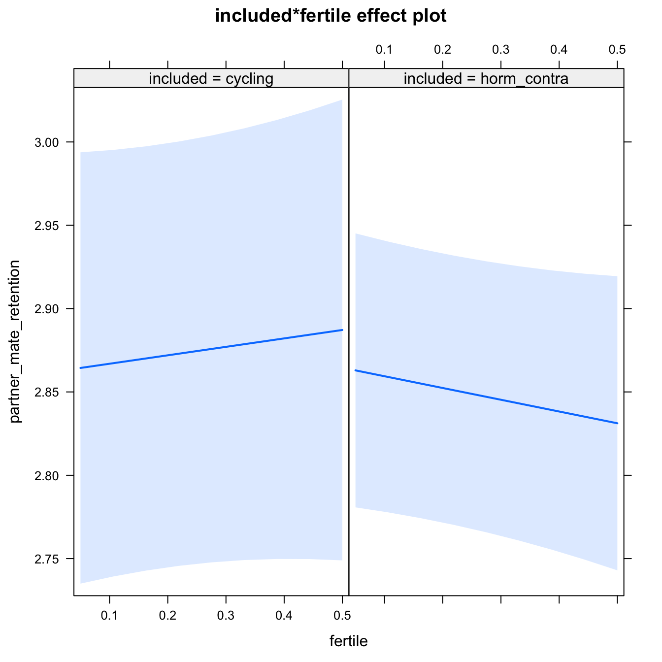
Diagnostics
model %>%
plot_outcome(diary) %>%
print_diagnostics()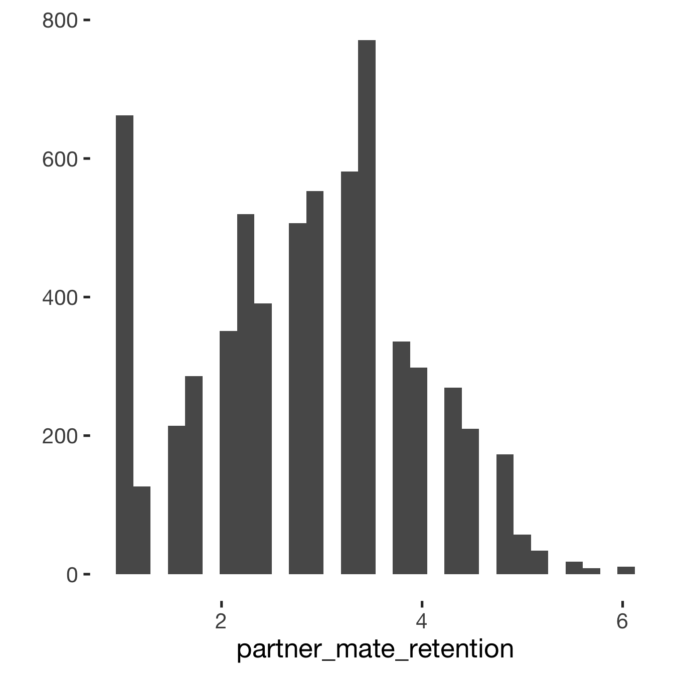
## Error in qqnorm.default(resid(obj)): y is empty or has only NAs
Adjusting for self esteem
model %>%
adjust_for_self_esteem(diary)##
##
## ```
## Linear mixed model fit by REML. t-tests use Satterthwaite's method ['lmerModLmerTest']
## Formula: form
## Data: diary
##
## REML criterion at convergence: 16223
##
## Scaled residuals:
## Min 1Q Median 3Q Max
## -3.744 -0.578 -0.007 0.602 4.310
##
## Random effects:
## Groups Name Variance Std.Dev.
## person (Intercept) 0.531 0.729
## Residual 0.615 0.784
## Number of obs: 6378, groups: person, 493
##
## Fixed effects:
## Estimate Std. Error df t value Pr(>|t|)
## (Intercept) 2.2543 0.0824 1179.2030 27.34 <2e-16 ***
## includedhorm_contra 0.0174 0.0788 556.0922 0.22 0.83
## fertile 0.0467 0.0878 5947.5671 0.53 0.60
## self_esteem_1 0.1415 0.0113 6367.2932 12.47 <2e-16 ***
## includedhorm_contra:fertile -0.1278 0.1051 5951.8238 -1.22 0.22
## ---
## Signif. codes: 0 '***' 0.001 '**' 0.01 '*' 0.05 '.' 0.1 ' ' 1
##
## Correlation of Fixed Effects:
## (Intr) incld_ fertil slf__1
## inclddhrm_c -0.688
## fertile -0.198 0.210
## self_estm_1 -0.591 0.013 -0.004
## inclddhrm_: 0.170 -0.251 -0.835 -0.005
##
## ```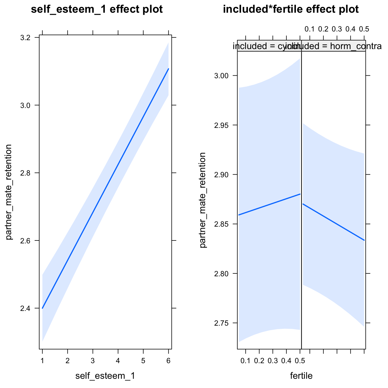
Broad window
outcome = names(model@frame)[1]
broad_models[[outcome]] <<- model %>%
switch_window_to_broad(diary)Linear mixed model fit by REML. t-tests use Satterthwaite's method ['lmerModLmerTest']
Formula: form
Data: diary2
REML criterion at convergence: 19662
Scaled residuals:
Min 1Q Median 3Q Max
-3.982 -0.604 0.007 0.621 4.579
Random effects:
Groups Name Variance Std.Dev.
person (Intercept) 0.543 0.737
Residual 0.628 0.792
Number of obs: 7740, groups: person, 493
Fixed effects:
Estimate Std. Error df t value Pr(>|t|)
(Intercept) 2.86102 0.06730 572.78868 42.51 <2e-16 ***
includedhorm_contra 0.00406 0.07976 576.16327 0.05 0.96
fertile 0.02199 0.08893 7325.49681 0.25 0.80
includedhorm_contra:fertile -0.11222 0.10624 7331.24430 -1.06 0.29
---
Signif. codes: 0 '***' 0.001 '**' 0.01 '*' 0.05 '.' 0.1 ' ' 1
Correlation of Fixed Effects:
(Intr) incld_ fertil
inclddhrm_c -0.844
fertile -0.277 0.234
inclddhrm_: 0.232 -0.280 -0.837
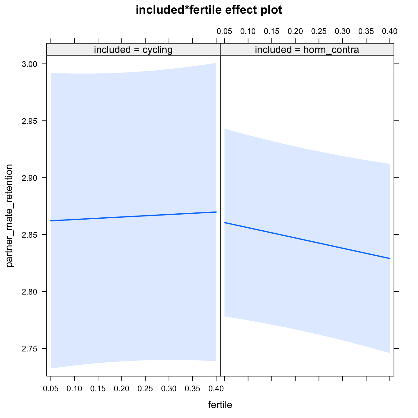
Diagnostics
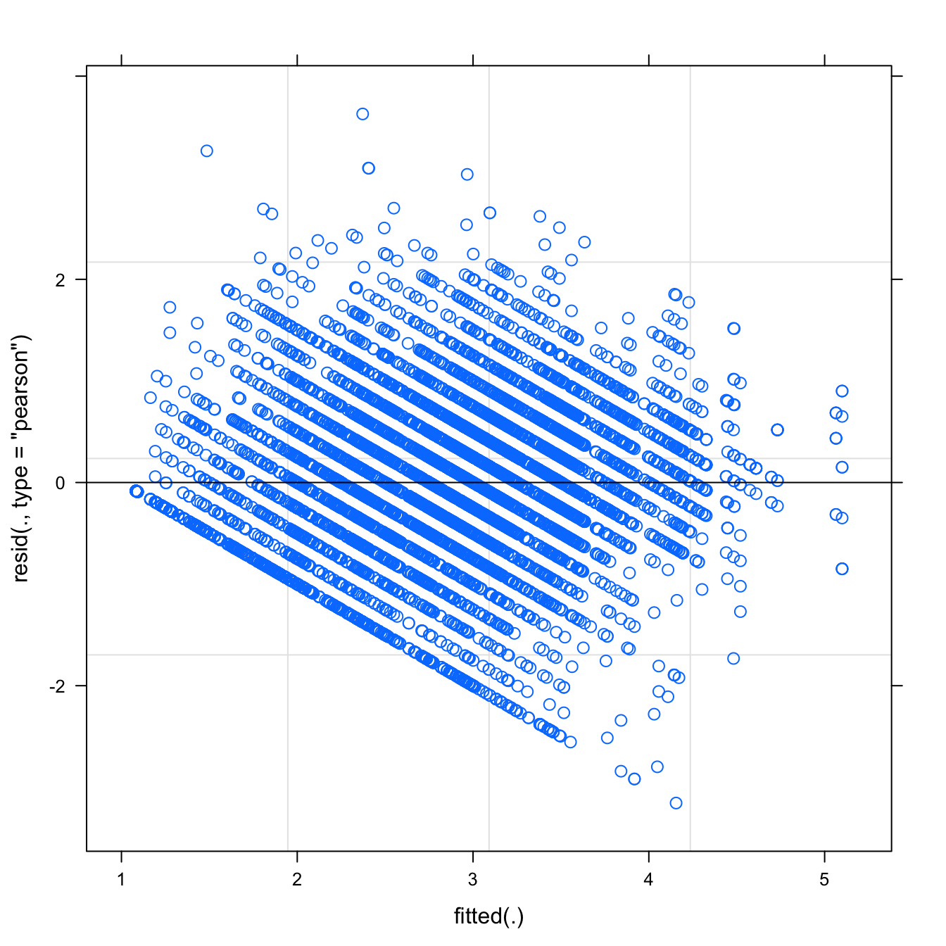
## Warning: 'sjp.lmer' is deprecated.
## Use 'plot_model' instead.
## See help("Deprecated")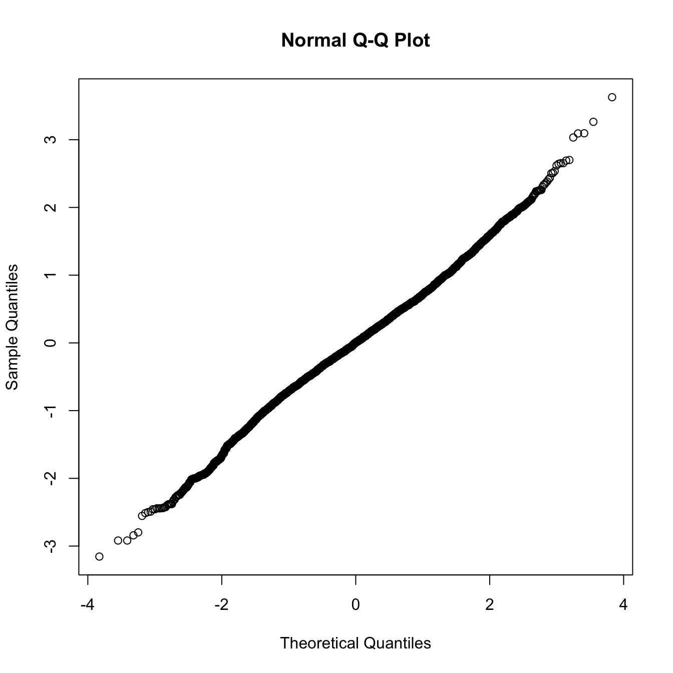
## Warning: 'sjp.lmer' is deprecated.
## Use 'plot_model' instead.
## See help("Deprecated")
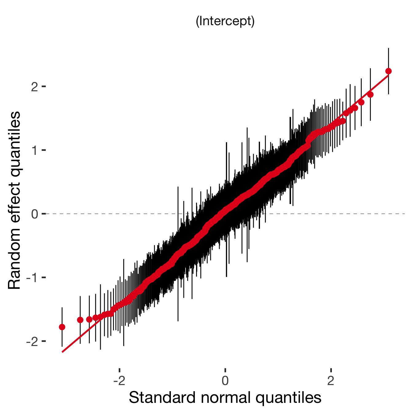
Adjusting for self esteem
broad_models[[outcome]] %>%
adjust_for_self_esteem(diary2)##
##
## ```
## Linear mixed model fit by REML. t-tests use Satterthwaite's method ['lmerModLmerTest']
## Formula: form
## Data: diary
##
## REML criterion at convergence: 19487
##
## Scaled residuals:
## Min 1Q Median 3Q Max
## -4.060 -0.590 -0.010 0.613 4.584
##
## Random effects:
## Groups Name Variance Std.Dev.
## person (Intercept) 0.536 0.732
## Residual 0.613 0.783
## Number of obs: 7740, groups: person, 493
##
## Fixed effects:
## Estimate Std. Error df t value Pr(>|t|)
## (Intercept) 2.2633 0.0800 1099.9882 28.29 <2e-16 ***
## includedhorm_contra 0.0162 0.0792 575.0839 0.21 0.84
## fertile 0.0106 0.0879 7323.7958 0.12 0.90
## self_esteem_1 0.1392 0.0102 7724.6778 13.58 <2e-16 ***
## includedhorm_contra:fertile -0.1154 0.1050 7329.3383 -1.10 0.27
## ---
## Signif. codes: 0 '***' 0.001 '**' 0.01 '*' 0.05 '.' 0.1 ' ' 1
##
## Correlation of Fixed Effects:
## (Intr) incld_ fertil slf__1
## inclddhrm_c -0.711
## fertile -0.225 0.233
## self_estm_1 -0.550 0.011 -0.010
## inclddhrm_: 0.194 -0.279 -0.837 -0.002
##
## ```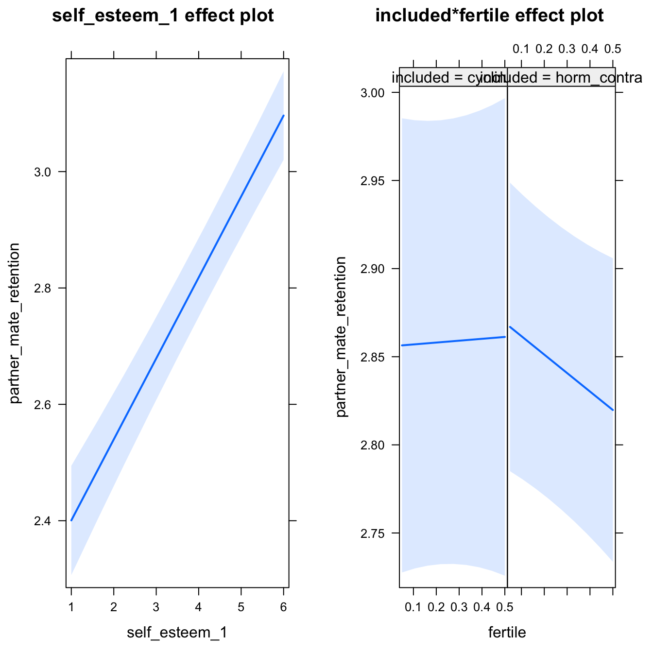
bla = 2do_moderators(models$partner_mate_retention, diary)Moderators
H2_1 Partner’s physical attractiveness
Predicted fertile phase effect sizes (in red): biggest (EP desire, partner mate retention)/smallest (IP desire) when partner’s physical attractiveness is low.
model %>%
test_moderator("partner_attractiveness_physical", diary)| Df | AIC | BIC | logLik | deviance | Chisq | Chi Df | Pr(>Chisq) | |
|---|---|---|---|---|---|---|---|---|
| with_main | 8 | 16363 | 16417 | -8174 | 16347 | NA | NA | NA |
| with_mod | 10 | 16366 | 16434 | -8173 | 16346 | 0.7181 | 2 | 0.6983 |
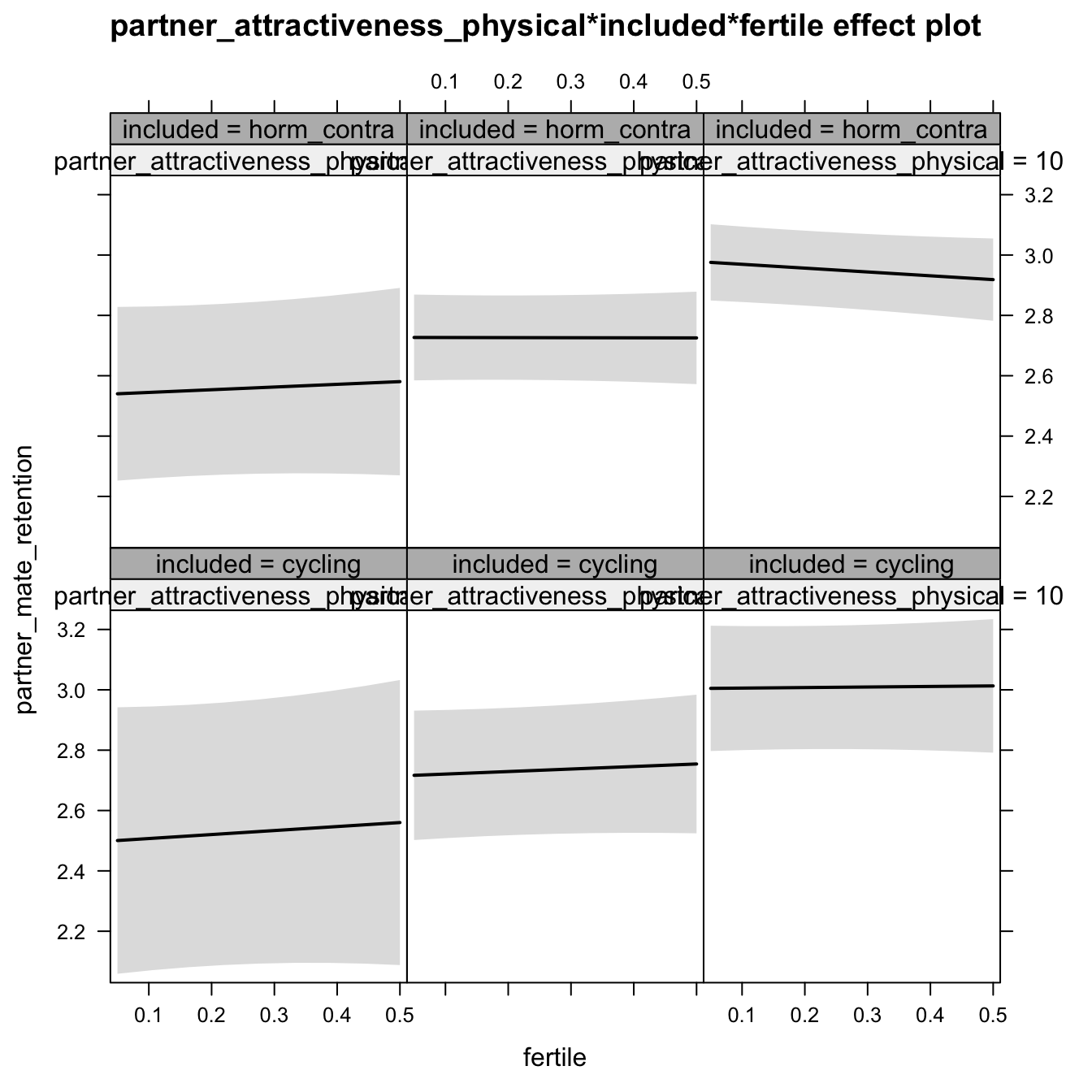
Linear mixed model fit by REML. t-tests use Satterthwaite's method ['lmerModLmerTest']
Formula: partner_mate_retention ~ (1 | person) + partner_attractiveness_physical +
included + fertile + partner_attractiveness_physical:included +
partner_attractiveness_physical:fertile + included:fertile +
partner_attractiveness_physical:included:fertile
Data: diary
REML criterion at convergence: 16380
Scaled residuals:
Min 1Q Median 3Q Max
-3.613 -0.593 -0.012 0.595 4.307
Random effects:
Groups Name Variance Std.Dev.
person (Intercept) 0.532 0.729
Residual 0.631 0.794
Number of obs: 6378, groups: person, 493
Fixed effects:
Estimate Std. Error df t value
(Intercept) 2.275368 0.354629 546.802838 6.42
partner_attractiveness_physical 0.072851 0.043267 547.876035 1.68
includedhorm_contra 0.069091 0.422519 551.616517 0.16
fertile 0.181471 0.466503 5938.039108 0.39
partner_attractiveness_physical:includedhorm_contra -0.009097 0.051305 552.856435 -0.18
partner_attractiveness_physical:fertile -0.016330 0.056840 5941.295112 -0.29
includedhorm_contra:fertile 0.000851 0.566975 5948.012993 0.00
partner_attractiveness_physical:includedhorm_contra:fertile -0.014599 0.068804 5950.196131 -0.21
Pr(>|t|)
(Intercept) 0.0000000003 ***
partner_attractiveness_physical 0.093 .
includedhorm_contra 0.870
fertile 0.697
partner_attractiveness_physical:includedhorm_contra 0.859
partner_attractiveness_physical:fertile 0.774
includedhorm_contra:fertile 0.999
partner_attractiveness_physical:includedhorm_contra:fertile 0.832
---
Signif. codes: 0 '***' 0.001 '**' 0.01 '*' 0.05 '.' 0.1 ' ' 1
Correlation of Fixed Effects:
(Intr) prtn__ incld_ fertil pr__:_ prt__: incl_:
prtnr_ttrc_ -0.982
inclddhrm_c -0.839 0.824
fertile -0.244 0.240 0.205
prtnr_tt_:_ 0.828 -0.843 -0.982 -0.203
prtnr_ttr_: 0.241 -0.246 -0.202 -0.982 0.207
inclddhrm_: 0.201 -0.198 -0.249 -0.823 0.244 0.808
prtnr_t_:_: -0.199 0.203 0.245 0.811 -0.249 -0.826 -0.982
H2_1 Partner’s short-term attractiveness
Predicted fertile phase effect sizes (in red): biggest (EP desire, partner mate retention)/smallest (IP desire) when partner’s short-term attractiveness is low.
model %>%
test_moderator("partner_attractiveness_shortterm", diary)| Df | AIC | BIC | logLik | deviance | Chisq | Chi Df | Pr(>Chisq) | |
|---|---|---|---|---|---|---|---|---|
| with_main | 8 | 16362 | 16417 | -8173 | 16346 | NA | NA | NA |
| with_mod | 10 | 16366 | 16434 | -8173 | 16346 | 0.04619 | 2 | 0.9772 |
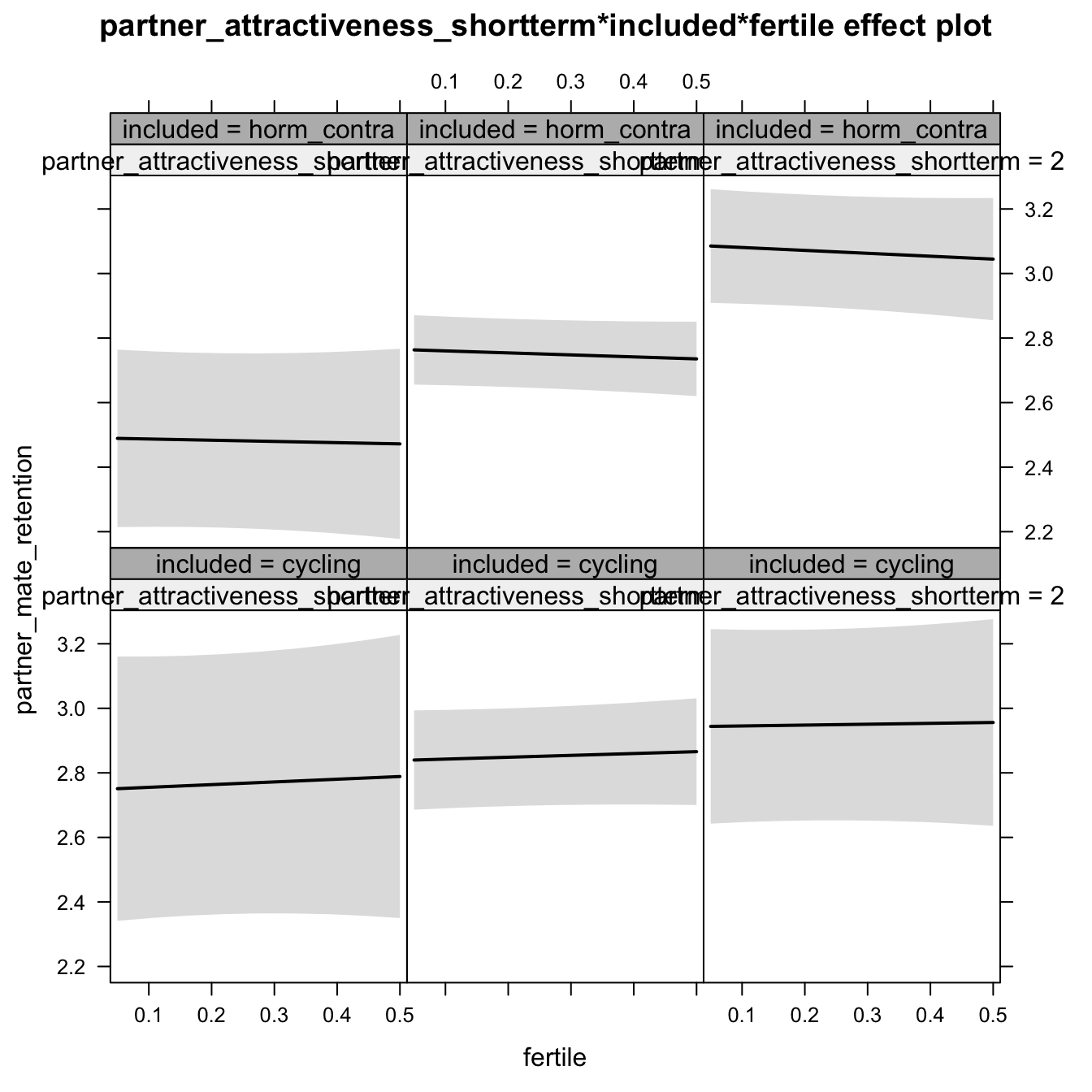
Linear mixed model fit by REML. t-tests use Satterthwaite's method ['lmerModLmerTest']
Formula: partner_mate_retention ~ (1 | person) + partner_attractiveness_shortterm +
included + fertile + partner_attractiveness_shortterm:included +
partner_attractiveness_shortterm:fertile + included:fertile +
partner_attractiveness_shortterm:included:fertile
Data: diary
REML criterion at convergence: 16376
Scaled residuals:
Min 1Q Median 3Q Max
-3.601 -0.592 -0.011 0.600 4.306
Random effects:
Groups Name Variance Std.Dev.
person (Intercept) 0.531 0.729
Residual 0.631 0.794
Number of obs: 6378, groups: person, 493
Fixed effects:
Estimate Std. Error df t value
(Intercept) 2.864267 0.066718 552.821948 42.93
partner_attractiveness_shortterm 0.039175 0.068513 563.497649 0.57
includedhorm_contra -0.014023 0.079238 555.442864 -0.18
fertile 0.049686 0.088990 5947.536862 0.56
partner_attractiveness_shortterm:includedhorm_contra 0.080565 0.081101 562.310833 0.99
partner_attractiveness_shortterm:fertile -0.011360 0.091590 5963.097746 -0.12
includedhorm_contra:fertile -0.118952 0.106737 5951.656225 -1.11
partner_attractiveness_shortterm:includedhorm_contra:fertile 0.000879 0.109188 5961.297564 0.01
Pr(>|t|)
(Intercept) <2e-16 ***
partner_attractiveness_shortterm 0.57
includedhorm_contra 0.86
fertile 0.58
partner_attractiveness_shortterm:includedhorm_contra 0.32
partner_attractiveness_shortterm:fertile 0.90
includedhorm_contra:fertile 0.27
partner_attractiveness_shortterm:includedhorm_contra:fertile 0.99
---
Signif. codes: 0 '***' 0.001 '**' 0.01 '*' 0.05 '.' 0.1 ' ' 1
Correlation of Fixed Effects:
(Intr) prtn__ incld_ fertil pr__:_ prt__: incl_:
prtnr_ttrc_ 0.063
inclddhrm_c -0.842 -0.053
fertile -0.252 -0.020 0.212
prtnr_tt_:_ -0.053 -0.845 0.005 0.017
prtnr_ttr_: -0.020 -0.256 0.017 0.043 0.216
inclddhrm_: 0.210 0.017 -0.254 -0.834 -0.005 -0.036
prtnr_t_:_: 0.017 0.215 -0.005 -0.036 -0.257 -0.839 -0.004
H2_1 Partner’s short-term vs long-term attractiveness
Predicted fertile phase effect sizes (in red): biggest (EP desire, partner mate retention)/smallest (IP desire) top-right (high LT, low ST), then top-left (low LT, low ST), then bottom-left (low LT, high ST), then bottom-right (high LT/ST).
add_main = update.formula(formula(model), new = as.formula(paste0(". ~ . + partner_attractiveness_longterm * included + partner_attractiveness_shortterm * included + partner_attractiveness_longterm * partner_attractiveness_shortterm"))) # reorder so that the triptych looks nice
add_mod_formula = update.formula(update.formula(formula(model), new = . ~ . - included * fertile), new = as.formula(paste0(". ~ . + partner_attractiveness_longterm * fertile * partner_attractiveness_shortterm * included"))) # reorder so that the triptych looks nice
update(model, formula = add_main) -> with_main
update(model, formula = add_mod_formula) -> with_mod
if (is(with_mod, "lmerMod")) {
  with_mod <- as_lmerModLmerTest(with_mod)
}
cat(pander(anova(with_main, with_mod)))| Df | AIC | BIC | logLik | deviance | Chisq | Chi Df | Pr(>Chisq) | |
|---|---|---|---|---|---|---|---|---|
| with_main | 11 | 16352 | 16426 | -8165 | 16330 | NA | NA | NA |
| with_mod | 18 | 16362 | 16484 | -8163 | 16326 | 3.375 | 7 | 0.8483 |
effs = allEffects(with_mod)
effs = data.frame(effs$`partner_attractiveness_longterm:fertile:partner_attractiveness_shortterm:included`) %>%
  filter(round(partner_attractiveness_longterm,1) %in% c(-3,-2,0.8),round(partner_attractiveness_shortterm,1) %in% c(-2,0.5, 2))
ggplot(effs, aes(fertile, fit, ymin = lower, ymax = upper, color = included)) +
  facet_grid(partner_attractiveness_shortterm ~ partner_attractiveness_longterm) +
  geom_smooth(stat='identity') +
  scale_color_manual(values = c("cycling" = 'red', 'horm_contra' = 'black'), guide = F) +
  scale_fill_manual(values = c("cycling" = 'red', 'horm_contra' = 'black'), guide = F) +
  ggtitle("Moderation", "top-to-bottom: short-term,\nleft-to-right: long-term attractiveness of the partner")+
  ylab(names(model@frame)[1])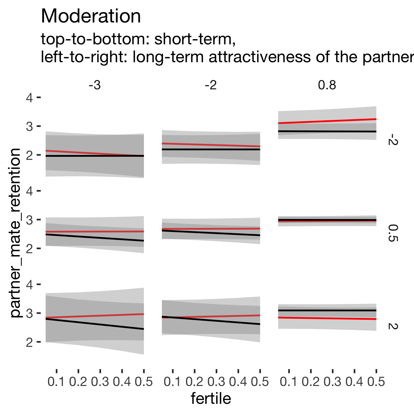
print_summary(with_mod)Linear mixed model fit by REML. t-tests use Satterthwaite's method ['lmerModLmerTest']
Formula: partner_mate_retention ~ (1 | person) + partner_attractiveness_longterm +
fertile + partner_attractiveness_shortterm + included + partner_attractiveness_longterm:fertile +
partner_attractiveness_longterm:partner_attractiveness_shortterm +
fertile:partner_attractiveness_shortterm + partner_attractiveness_longterm:included +
fertile:included + partner_attractiveness_shortterm:included +
partner_attractiveness_longterm:fertile:partner_attractiveness_shortterm +
partner_attractiveness_longterm:fertile:included + partner_attractiveness_longterm:partner_attractiveness_shortterm:included +
fertile:partner_attractiveness_shortterm:included + partner_attractiveness_longterm:fertile:partner_attractiveness_shortterm:included
Data: diary
REML criterion at convergence: 16385
Scaled residuals:
Min 1Q Median 3Q Max
-3.590 -0.586 -0.005 0.596 4.332
Random effects:
Groups Name Variance Std.Dev.
person (Intercept) 0.516 0.718
Residual 0.631 0.794
Number of obs: 6378, groups: person, 493
Fixed effects:
Estimate
(Intercept) 2.8682
partner_attractiveness_longterm 0.1239
fertile 0.0644
partner_attractiveness_shortterm -0.0120
includedhorm_contra -0.0273
partner_attractiveness_longterm:fertile 0.0446
partner_attractiveness_longterm:partner_attractiveness_shortterm -0.0593
fertile:partner_attractiveness_shortterm -0.0472
partner_attractiveness_longterm:includedhorm_contra 0.0228
fertile:includedhorm_contra -0.1566
partner_attractiveness_shortterm:includedhorm_contra 0.1110
partner_attractiveness_longterm:fertile:partner_attractiveness_shortterm -0.0731
partner_attractiveness_longterm:fertile:includedhorm_contra 0.0539
partner_attractiveness_longterm:partner_attractiveness_shortterm:includedhorm_contra 0.0195
fertile:partner_attractiveness_shortterm:includedhorm_contra 0.0106
partner_attractiveness_longterm:fertile:partner_attractiveness_shortterm:includedhorm_contra 0.1267
Std. Error
(Intercept) 0.0670
partner_attractiveness_longterm 0.0699
fertile 0.0905
partner_attractiveness_shortterm 0.0726
includedhorm_contra 0.0801
partner_attractiveness_longterm:fertile 0.0940
partner_attractiveness_longterm:partner_attractiveness_shortterm 0.0561
fertile:partner_attractiveness_shortterm 0.0984
partner_attractiveness_longterm:includedhorm_contra 0.0875
fertile:includedhorm_contra 0.1096
partner_attractiveness_shortterm:includedhorm_contra 0.0852
partner_attractiveness_longterm:fertile:partner_attractiveness_shortterm 0.0775
partner_attractiveness_longterm:fertile:includedhorm_contra 0.1223
partner_attractiveness_longterm:partner_attractiveness_shortterm:includedhorm_contra 0.0788
fertile:partner_attractiveness_shortterm:includedhorm_contra 0.1166
partner_attractiveness_longterm:fertile:partner_attractiveness_shortterm:includedhorm_contra 0.1112
df
(Intercept) 547.2833
partner_attractiveness_longterm 536.1745
fertile 5942.0304
partner_attractiveness_shortterm 563.2459
includedhorm_contra 551.1075
partner_attractiveness_longterm:fertile 5927.6742
partner_attractiveness_longterm:partner_attractiveness_shortterm 544.1130
fertile:partner_attractiveness_shortterm 5970.9835
partner_attractiveness_longterm:includedhorm_contra 545.6717
fertile:includedhorm_contra 5951.4946
partner_attractiveness_shortterm:includedhorm_contra 562.1603
partner_attractiveness_longterm:fertile:partner_attractiveness_shortterm 5946.0173
partner_attractiveness_longterm:fertile:includedhorm_contra 5958.6967
partner_attractiveness_longterm:partner_attractiveness_shortterm:includedhorm_contra 549.5921
fertile:partner_attractiveness_shortterm:includedhorm_contra 5971.2524
partner_attractiveness_longterm:fertile:partner_attractiveness_shortterm:includedhorm_contra 5967.0384
t value Pr(>|t|)
(Intercept) 42.80 <2e-16
partner_attractiveness_longterm 1.77 0.077
fertile 0.71 0.477
partner_attractiveness_shortterm -0.17 0.868
includedhorm_contra -0.34 0.734
partner_attractiveness_longterm:fertile 0.47 0.635
partner_attractiveness_longterm:partner_attractiveness_shortterm -1.06 0.291
fertile:partner_attractiveness_shortterm -0.48 0.632
partner_attractiveness_longterm:includedhorm_contra 0.26 0.795
fertile:includedhorm_contra -1.43 0.153
partner_attractiveness_shortterm:includedhorm_contra 1.30 0.193
partner_attractiveness_longterm:fertile:partner_attractiveness_shortterm -0.94 0.345
partner_attractiveness_longterm:fertile:includedhorm_contra 0.44 0.660
partner_attractiveness_longterm:partner_attractiveness_shortterm:includedhorm_contra 0.25 0.805
fertile:partner_attractiveness_shortterm:includedhorm_contra 0.09 0.928
partner_attractiveness_longterm:fertile:partner_attractiveness_shortterm:includedhorm_contra 1.14 0.254
(Intercept) ***
partner_attractiveness_longterm .
fertile
partner_attractiveness_shortterm
includedhorm_contra
partner_attractiveness_longterm:fertile
partner_attractiveness_longterm:partner_attractiveness_shortterm
fertile:partner_attractiveness_shortterm
partner_attractiveness_longterm:includedhorm_contra
fertile:includedhorm_contra
partner_attractiveness_shortterm:includedhorm_contra
partner_attractiveness_longterm:fertile:partner_attractiveness_shortterm
partner_attractiveness_longterm:fertile:includedhorm_contra
partner_attractiveness_longterm:partner_attractiveness_shortterm:includedhorm_contra
fertile:partner_attractiveness_shortterm:includedhorm_contra
partner_attractiveness_longterm:fertile:partner_attractiveness_shortterm:includedhorm_contra
---
Signif. codes: 0 '***' 0.001 '**' 0.01 '*' 0.05 '.' 0.1 ' ' 1
H2_1b Partner’s short-term and long-term attractiveness
Edit: Alternative model specification, added after publication. Predicted fertile phase effect sizes (in red): biggest (EP desire, partner mate retention)/smallest (IP desire) top-right (high LT, low ST), then top-left (low LT, low ST), then bottom-left (low LT, high ST), then bottom-right (high LT/ST).
add_main = update.formula(formula(model), new = as.formula(paste0(". ~ . + partner_attractiveness_shortterm * included + partner_attractiveness_longterm * fertile * included"))) # reorder so that the triptych looks nice
add_mod_formula = update.formula(update.formula(formula(model), new = . ~ . - included * fertile), new = as.formula(paste0(". ~ . + (partner_attractiveness_shortterm + partner_attractiveness_longterm) * fertile * included"))) # reorder so that the triptych looks nice

update(model, formula = add_main) -> with_main
update(model, formula = add_mod_formula) -> with_mod
if (is(with_mod, "lmerMod")) {
  with_mod <- as_lmerModLmerTest(with_mod)
}
cat(pander(anova(with_main, with_mod)))| Df | AIC | BIC | logLik | deviance | Chisq | Chi Df | Pr(>Chisq) | |
|---|---|---|---|---|---|---|---|---|
| with_main | 12 | 16354 | 16435 | -8165 | 16330 | NA | NA | NA |
| with_mod | 14 | 16358 | 16452 | -8165 | 16330 | 0.2579 | 2 | 0.879 |
plot_triptych(with_mod)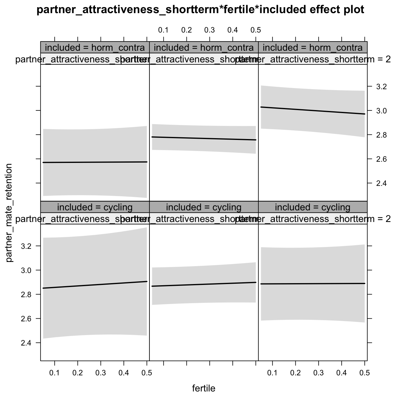
print_summary(with_mod)Linear mixed model fit by REML. t-tests use Satterthwaite's method ['lmerModLmerTest']
Formula: partner_mate_retention ~ (1 | person) + partner_attractiveness_shortterm +
partner_attractiveness_longterm + fertile + included + partner_attractiveness_shortterm:fertile +
partner_attractiveness_longterm:fertile + partner_attractiveness_shortterm:included +
partner_attractiveness_longterm:included + fertile:included +
partner_attractiveness_shortterm:fertile:included + partner_attractiveness_longterm:fertile:included
Data: diary
REML criterion at convergence: 16374
Scaled residuals:
Min 1Q Median 3Q Max
-3.594 -0.589 -0.010 0.598 4.332
Random effects:
Groups Name Variance Std.Dev.
person (Intercept) 0.516 0.719
Residual 0.631 0.794
Number of obs: 6378, groups: person, 493
Fixed effects:
Estimate Std. Error df t value
(Intercept) 2.85603 0.06606 552.26098 43.23
partner_attractiveness_shortterm 0.00817 0.06965 561.77335 0.12
partner_attractiveness_longterm 0.13311 0.06942 540.16773 1.92
fertile 0.04858 0.08900 5946.64815 0.55
includedhorm_contra -0.02239 0.07864 554.99880 -0.28
partner_attractiveness_shortterm:fertile -0.02289 0.09428 5960.92407 -0.24
partner_attractiveness_longterm:fertile 0.05114 0.09367 5930.66044 0.55
partner_attractiveness_shortterm:includedhorm_contra 0.08476 0.08236 561.46711 1.03
partner_attractiveness_longterm:includedhorm_contra 0.01614 0.08712 548.89793 0.19
fertile:includedhorm_contra -0.13017 0.10719 5952.62066 -1.21
partner_attractiveness_shortterm:fertile:includedhorm_contra -0.00448 0.11239 5961.40874 -0.04
partner_attractiveness_longterm:fertile:includedhorm_contra 0.04053 0.12156 5958.09063 0.33
Pr(>|t|)
(Intercept) <2e-16 ***
partner_attractiveness_shortterm 0.907
partner_attractiveness_longterm 0.056 .
fertile 0.585
includedhorm_contra 0.776
partner_attractiveness_shortterm:fertile 0.808
partner_attractiveness_longterm:fertile 0.585
partner_attractiveness_shortterm:includedhorm_contra 0.304
partner_attractiveness_longterm:includedhorm_contra 0.853
fertile:includedhorm_contra 0.225
partner_attractiveness_shortterm:fertile:includedhorm_contra 0.968
partner_attractiveness_longterm:fertile:includedhorm_contra 0.739
---
Signif. codes: 0 '***' 0.001 '**' 0.01 '*' 0.05 '.' 0.1 ' ' 1
Correlation of Fixed Effects:
(Intr) prtnr_ttrctvnss_s prtnr_ttrctvnss_l fertil incld_ prtnr_ttrctvnss_s:
prtnr_ttrctvnss_s 0.075
prtnr_ttrctvnss_l -0.059 -0.234
fertile -0.255 -0.021 0.004
inclddhrm_c -0.840 -0.063 0.050 0.214
prtnr_ttrctvnss_s: -0.021 -0.259 0.060 0.047 0.017
prtnr_ttrctvnss_l: 0.003 0.060 -0.245 -0.019 -0.003 -0.238
prtnr_ttrctvnss_s:_ -0.063 -0.846 0.198 0.017 0.024 0.219
prtnr_ttrctvnss_l:_ 0.047 0.186 -0.797 -0.003 -0.085 -0.048
frtl:ncldd_ 0.211 0.017 -0.003 -0.830 -0.257 -0.039
prtnr_ttrctvnss_s::_ 0.017 0.217 -0.050 -0.039 -0.008 -0.839
prtnr_ttrctvnss_l::_ -0.003 -0.046 0.189 0.014 0.015 0.183
prtnr_ttrctvnss_l: prtnr_ttrctvnss_s:_ prtnr_ttrctvnss_l:_ frtl:_ prtnr_ttrctvnss_s::_
prtnr_ttrctvnss_s
prtnr_ttrctvnss_l
fertile
inclddhrm_c
prtnr_ttrctvnss_s:
prtnr_ttrctvnss_l:
prtnr_ttrctvnss_s:_ -0.051
prtnr_ttrctvnss_l:_ 0.195 -0.228
frtl:ncldd_ 0.015 -0.008 0.016
prtnr_ttrctvnss_s::_ 0.199 -0.260 0.061 0.011
prtnr_ttrctvnss_l::_ -0.771 0.059 -0.250 -0.071 -0.236
H2_1c Partner’s short-term minus long-term attractiveness
Edit: Alternative model specification, added after publication. Predicted fertile phase effect sizes (in red): biggest (EP desire, partner mate retention)/smallest (IP desire) top-right (high LT, low ST), then top-left (low LT, low ST), then bottom-left (low LT, high ST), then bottom-right (high LT/ST).
add_main = update.formula(formula(model), new = as.formula(paste0(". ~ . + partner_st_vs_lt * included"))) # reorder so that the triptych looks nice
add_mod_formula = update.formula(update.formula(formula(model), new = . ~ . - included * fertile), new = as.formula(paste0(". ~ . + partner_st_vs_lt * fertile * included"))) # reorder so that the triptych looks nice

update(model, formula = add_main) -> with_main
update(model, formula = add_mod_formula) -> with_mod
if (is(with_mod, "lmerMod")) {
  with_mod <- as_lmerModLmerTest(with_mod)
}
cat(pander(anova(with_main, with_mod)))| Df | AIC | BIC | logLik | deviance | Chisq | Chi Df | Pr(>Chisq) | |
|---|---|---|---|---|---|---|---|---|
| with_main | 8 | 16369 | 16423 | -8176 | 16353 | NA | NA | NA |
| with_mod | 10 | 16372 | 16439 | -8176 | 16352 | 1.052 | 2 | 0.591 |
plot_triptych(with_mod)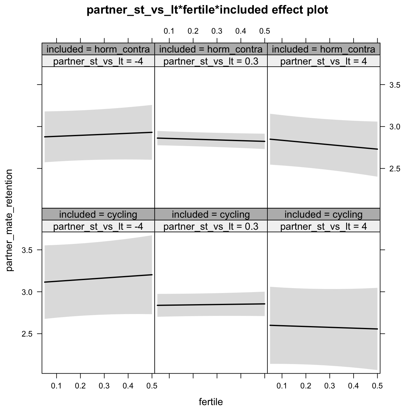
print_summary(with_mod)Linear mixed model fit by REML. t-tests use Satterthwaite's method ['lmerModLmerTest']
Formula: partner_mate_retention ~ (1 | person) + partner_st_vs_lt + fertile +
included + partner_st_vs_lt:fertile + partner_st_vs_lt:included +
fertile:included + partner_st_vs_lt:fertile:included
Data: diary
REML criterion at convergence: 16383
Scaled residuals:
Min 1Q Median 3Q Max
-3.593 -0.591 -0.005 0.598 4.303
Random effects:
Groups Name Variance Std.Dev.
person (Intercept) 0.539 0.734
Residual 0.631 0.794
Number of obs: 6378, groups: person, 493
Fixed effects:
Estimate Std. Error df t value Pr(>|t|)
(Intercept) 2.8551 0.0673 551.5114 42.44 <2e-16 ***
partner_st_vs_lt -0.0626 0.0556 547.4562 -1.12 0.26
fertile 0.0494 0.0890 5945.9341 0.56 0.58
includedhorm_contra 0.0116 0.0796 554.7566 0.15 0.88
partner_st_vs_lt:fertile -0.0365 0.0739 5942.3716 -0.49 0.62
partner_st_vs_lt:includedhorm_contra 0.0615 0.0673 552.3116 0.91 0.36
fertile:includedhorm_contra -0.1217 0.1065 5950.9138 -1.14 0.25
partner_st_vs_lt:fertile:includedhorm_contra -0.0113 0.0911 5955.9740 -0.12 0.90
---
Signif. codes: 0 '***' 0.001 '**' 0.01 '*' 0.05 '.' 0.1 ' ' 1
Correlation of Fixed Effects:
(Intr) prt___ fertil incld_ pr___: p___:_ frtl:_
prtnr_st_v_ 0.085
fertile -0.250 -0.015
inclddhrm_c -0.845 -0.072 0.211
prtnr_st__: -0.015 -0.248 0.041 0.013
prtnr_s__:_ -0.070 -0.827 0.012 0.060 0.205
frtl:ncldd_ 0.209 0.013 -0.835 -0.252 -0.034 -0.012
prtnr___::_ 0.012 0.201 -0.033 -0.012 -0.812 -0.251 0.038
H2_3 Relative attractiveness to self
Predicted fertile phase effect sizes (in red): biggest (EP desire, partner mate retention)/smallest (IP desire) when partner’s relative attractiveness is low.
model %>%
test_moderator("partner_attractiveness_rel_to_self", diary)| Df | AIC | BIC | logLik | deviance | Chisq | Chi Df | Pr(>Chisq) | |
|---|---|---|---|---|---|---|---|---|
| with_main | 8 | 16370 | 16424 | -8177 | 16354 | NA | NA | NA |
| with_mod | 10 | 16369 | 16436 | -8174 | 16349 | 5.151 | 2 | 0.07613 |
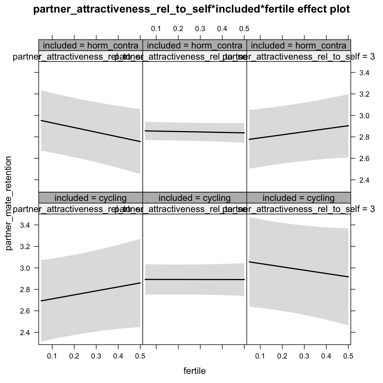
Linear mixed model fit by REML. t-tests use Satterthwaite's method ['lmerModLmerTest']
Formula: partner_mate_retention ~ (1 | person) + partner_attractiveness_rel_to_self +
included + fertile + partner_attractiveness_rel_to_self:included +
partner_attractiveness_rel_to_self:fertile + included:fertile +
partner_attractiveness_rel_to_self:included:fertile
Data: diary
REML criterion at convergence: 16379
Scaled residuals:
Min 1Q Median 3Q Max
-3.630 -0.583 -0.008 0.596 4.308
Random effects:
Groups Name Variance Std.Dev.
person (Intercept) 0.54 0.735
Residual 0.63 0.794
Number of obs: 6378, groups: person, 493
Fixed effects:
Estimate Std. Error df t value
(Intercept) 2.87269 0.06785 552.40389 42.34
partner_attractiveness_rel_to_self 0.06614 0.06491 550.65695 1.02
includedhorm_contra -0.00446 0.08016 555.25600 -0.06
fertile 0.03104 0.09026 5948.84440 0.34
partner_attractiveness_rel_to_self:includedhorm_contra -0.10127 0.07936 554.80641 -1.28
partner_attractiveness_rel_to_self:fertile -0.11339 0.09125 5969.51419 -1.24
includedhorm_contra:fertile -0.10760 0.10762 5952.60373 -1.00
partner_attractiveness_rel_to_self:includedhorm_contra:fertile 0.23276 0.11082 5967.53851 2.10
Pr(>|t|)
(Intercept) <2e-16 ***
partner_attractiveness_rel_to_self 0.309
includedhorm_contra 0.956
fertile 0.731
partner_attractiveness_rel_to_self:includedhorm_contra 0.202
partner_attractiveness_rel_to_self:fertile 0.214
includedhorm_contra:fertile 0.317
partner_attractiveness_rel_to_self:includedhorm_contra:fertile 0.036 *
---
Signif. codes: 0 '***' 0.001 '**' 0.01 '*' 0.05 '.' 0.1 ' ' 1
Correlation of Fixed Effects:
(Intr) pr____ incld_ fertil pr____:_ pr____: incl_:
prtnr_tt___ 0.153
inclddhrm_c -0.846 -0.129
fertile -0.250 -0.043 0.212
prtnr____:_ -0.125 -0.818 0.091 0.036
prtnr_t___: -0.041 -0.247 0.035 0.175 0.202
inclddhrm_: 0.210 0.036 -0.252 -0.839 -0.025 -0.147
prtn____:_: 0.034 0.204 -0.025 -0.144 -0.249 -0.823 0.104
H1.7. Narcisstic admiration
models$NARQ_admiration = lmer(NARQ_admiration ~ included * fertile + ( 1 | person), data = diary)
do_model(models$NARQ_admiration, diary)Narrow window
model %>%
  print_summary() %>%
plot_all_effects()Linear mixed model fit by REML. t-tests use Satterthwaite's method ['lmerModLmerTest']
Formula: NARQ_admiration ~ included * fertile + (1 | person)
Data: diary
REML criterion at convergence: 15320
Scaled residuals:
Min 1Q Median 3Q Max
-5.570 -0.487 -0.093 0.527 4.593
Random effects:
Groups Name Variance Std.Dev.
person (Intercept) 1.208 1.099
Residual 0.496 0.704
Number of obs: 6378, groups: person, 493
Fixed effects:
Estimate Std. Error df t value Pr(>|t|)
(Intercept) 2.6854 0.0954 515.0024 28.14 <2e-16 ***
includedhorm_contra -0.1406 0.1130 516.0786 -1.24 0.21
fertile -0.0471 0.0790 5910.9228 -0.60 0.55
includedhorm_contra:fertile -0.0911 0.0946 5912.3726 -0.96 0.34
---
Signif. codes: 0 '***' 0.001 '**' 0.01 '*' 0.05 '.' 0.1 ' ' 1
Correlation of Fixed Effects:
(Intr) incld_ fertil
inclddhrm_c -0.845
fertile -0.156 0.131
inclddhrm_: 0.130 -0.157 -0.835
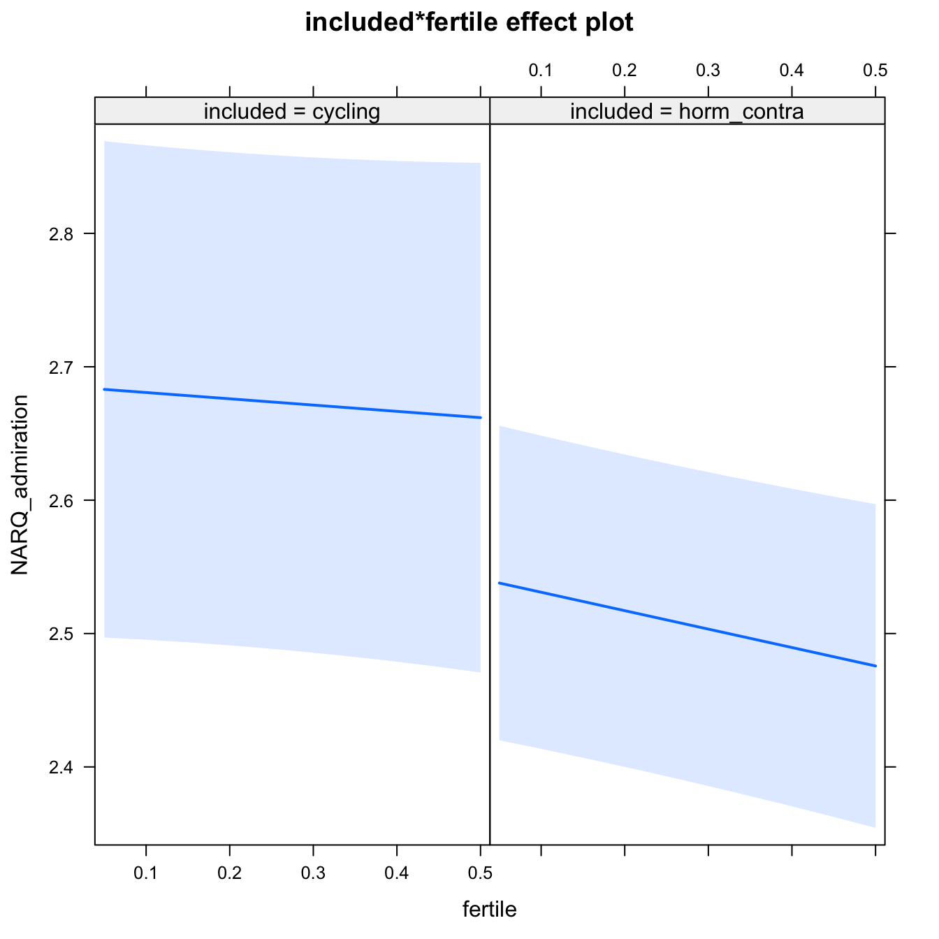
Diagnostics
model %>%
  plot_outcome(diary) %>%
  print_diagnostics()
## Error in qqnorm.default(resid(obj)): y is empty or has only NAs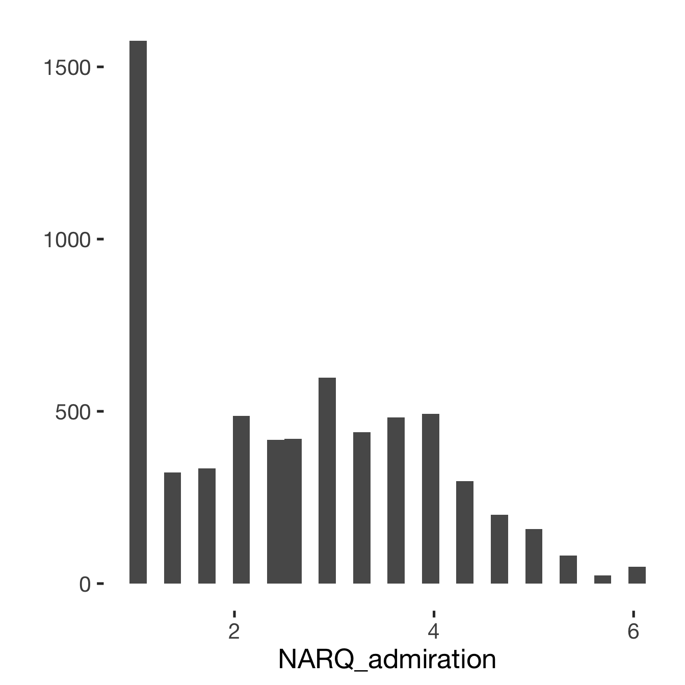
Adjusting for self esteem
model %>%
  adjust_for_self_esteem(diary)
##
##
## ```
## Linear mixed model fit by REML. t-tests use Satterthwaite's method ['lmerModLmerTest']
## Formula: form
## Data: diary
##
## REML criterion at convergence: 14158
##
## Scaled residuals:
## Min 1Q Median 3Q Max
## -5.833 -0.574 -0.057 0.566 4.606
##
## Random effects:
## Groups Name Variance Std.Dev.
## person (Intercept) 1.071 1.035
## Residual 0.411 0.641
## Number of obs: 6378, groups: person, 493
##
## Fixed effects:
## Estimate Std. Error df t value Pr(>|t|)
## (Intercept) 1.22661 0.09850 734.49210 12.45 <2e-16 ***
## includedhorm_contra -0.11043 0.10620 513.55005 -1.04 0.30
## fertile -0.05738 0.07187 5907.42075 -0.80 0.42
## self_esteem_1 0.33989 0.00948 6143.23935 35.84 <2e-16 ***
## includedhorm_contra:fertile -0.10691 0.08607 5908.75832 -1.24 0.21
## ---
## Signif. codes: 0 '***' 0.001 '**' 0.01 '*' 0.05 '.' 0.1 ' ' 1
##
## Correlation of Fixed Effects:
## (Intr) incld_ fertil slf__1
## inclddhrm_c -0.772
## fertile -0.136 0.127
## self_estm_1 -0.413 0.008 -0.004
## inclddhrm_: 0.117 -0.152 -0.835 -0.005
##
## ```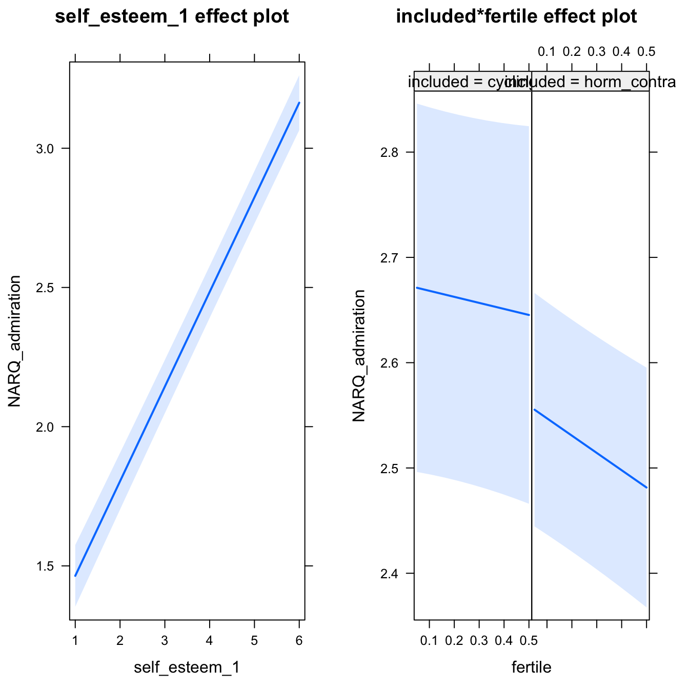
Broad window
outcome = names(model@frame)[1]
broad_models[[outcome]] <<- model %>%
switch_window_to_broad(diary)Linear mixed model fit by REML. t-tests use Satterthwaite's method ['lmerModLmerTest']
Formula: form
Data: diary2
REML criterion at convergence: 18438
Scaled residuals:
Min 1Q Median 3Q Max
-5.653 -0.488 -0.082 0.546 4.733
Random effects:
Groups Name Variance Std.Dev.
person (Intercept) 1.190 1.09
Residual 0.504 0.71
Number of obs: 7740, groups: person, 493
Fixed effects:
Estimate Std. Error df t value Pr(>|t|)
(Intercept) 2.682321 0.094853 523.037094 28.28 <2e-16 ***
includedhorm_contra -0.136206 0.112315 524.203288 -1.21 0.23
fertile -0.000987 0.079865 7280.199242 -0.01 0.99
includedhorm_contra:fertile -0.134464 0.095425 7282.535433 -1.41 0.16
---
Signif. codes: 0 '***' 0.001 '**' 0.01 '*' 0.05 '.' 0.1 ' ' 1
Correlation of Fixed Effects:
(Intr) incld_ fertil
inclddhrm_c -0.845
fertile -0.176 0.149
inclddhrm_: 0.147 -0.178 -0.837
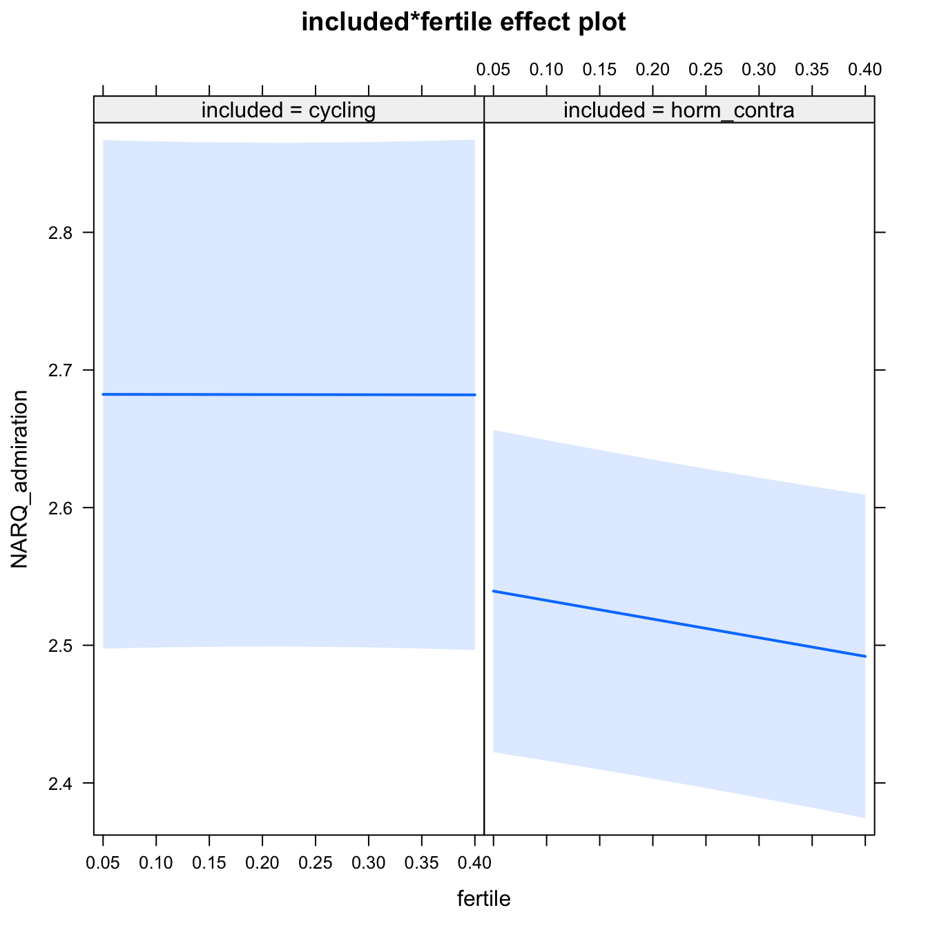
Diagnostics
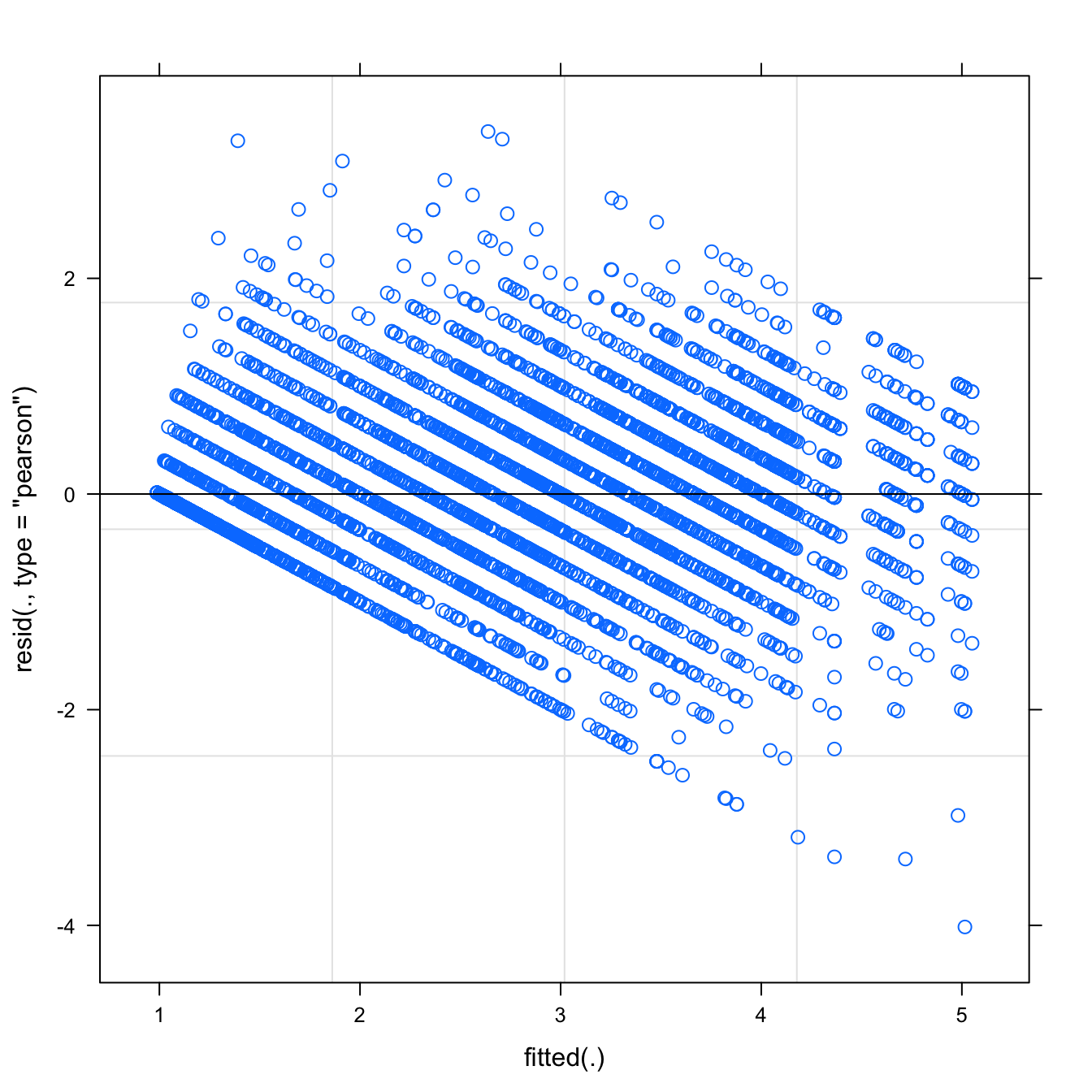
## Warning: 'sjp.lmer' is deprecated.
## Use 'plot_model' instead.
## See help("Deprecated")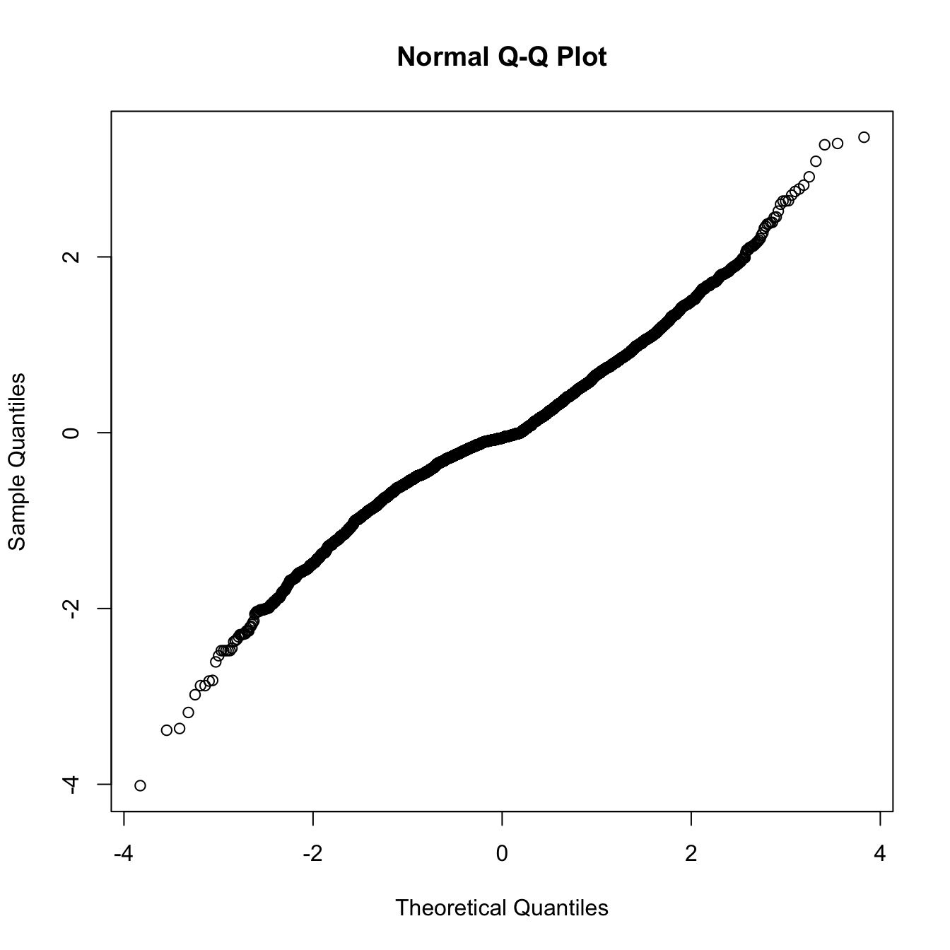
## Warning: 'sjp.lmer' is deprecated.
## Use 'plot_model' instead.
## See help("Deprecated")
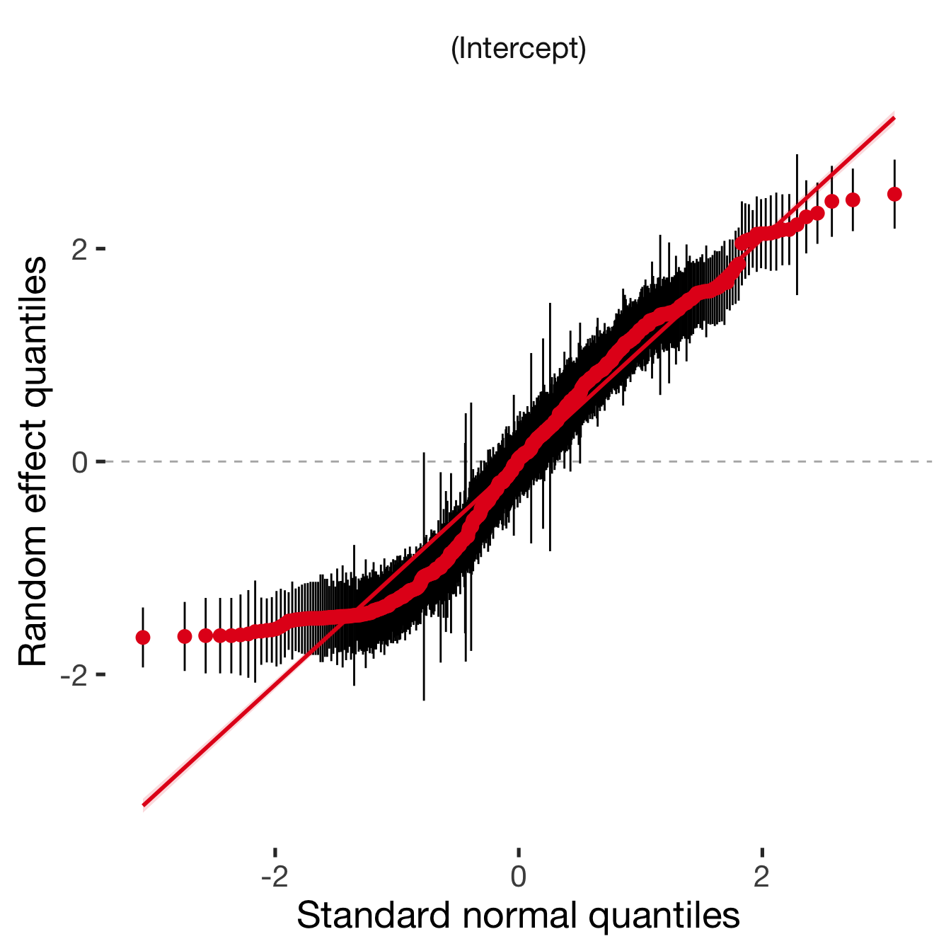
Adjusting for self esteem
broad_models[[outcome]] %>%
adjust_for_self_esteem(diary2)##
##
## ```
## Linear mixed model fit by REML. t-tests use Satterthwaite's method ['lmerModLmerTest']
## Formula: form
## Data: diary
##
## REML criterion at convergence: 17050
##
## Scaled residuals:
## Min 1Q Median 3Q Max
## -5.881 -0.570 -0.061 0.562 4.745
##
## Random effects:
## Groups Name Variance Std.Dev.
## person (Intercept) 1.05 1.027
## Residual 0.42 0.648
## Number of obs: 7740, groups: person, 493
##
## Fixed effects:
## Estimate Std. Error df t value Pr(>|t|)
## (Intercept) 1.23284 0.09649 708.42566 12.78 <2e-16 ***
## includedhorm_contra -0.10697 0.10550 521.26889 -1.01 0.31
## fertile -0.02940 0.07285 7276.47942 -0.40 0.69
## self_esteem_1 0.33760 0.00863 7503.76259 39.13 <2e-16 ***
## includedhorm_contra:fertile -0.14153 0.08704 7278.61177 -1.63 0.10
## ---
## Signif. codes: 0 '***' 0.001 '**' 0.01 '*' 0.05 '.' 0.1 ' ' 1
##
## Correlation of Fixed Effects:
## (Intr) incld_ fertil slf__1
## inclddhrm_c -0.783
## fertile -0.154 0.144
## self_estm_1 -0.384 0.007 -0.010
## inclddhrm_: 0.133 -0.173 -0.837 -0.002
##
## ```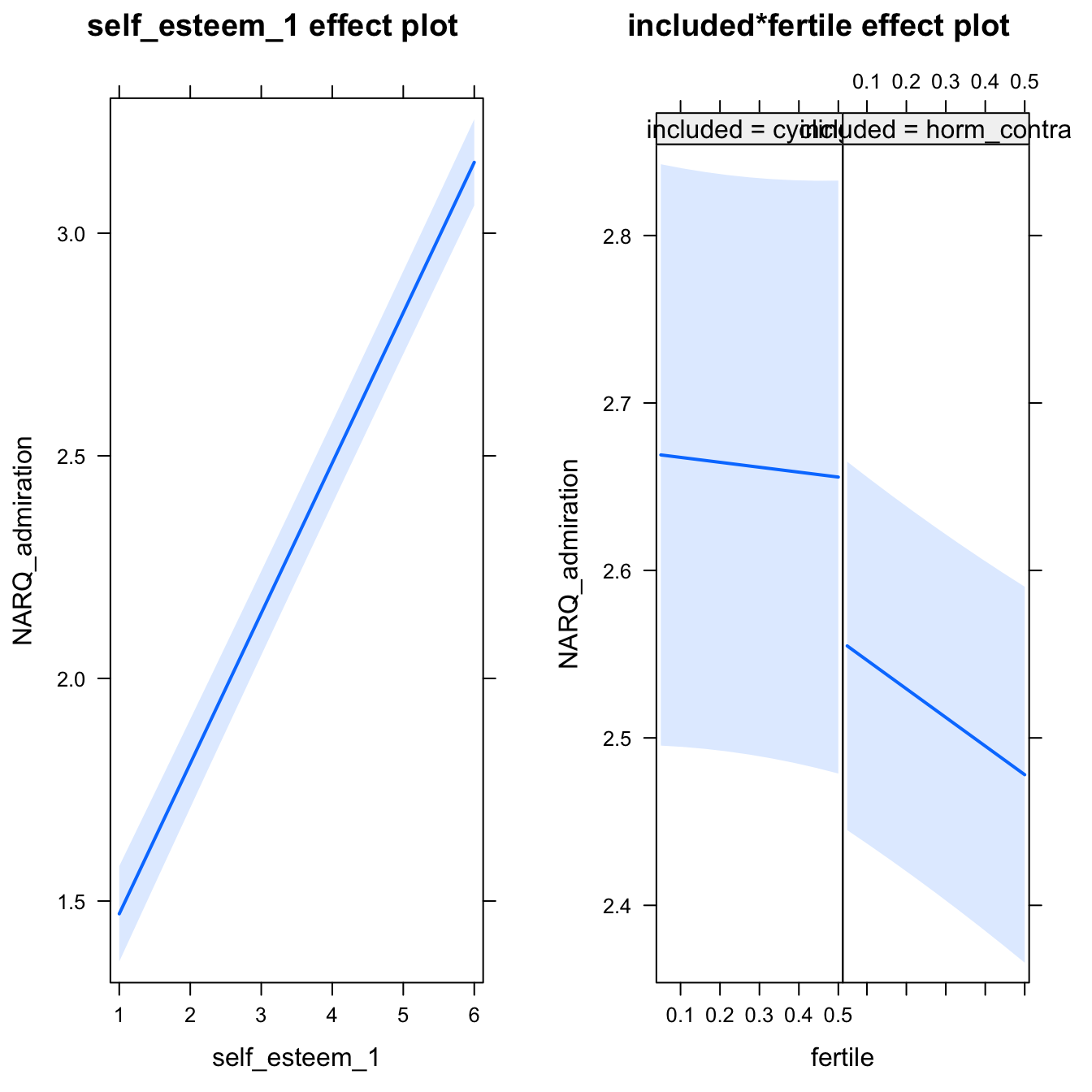
bla = 2H1.7. Narcisstic rivalry
models$NARQ_rivalry = lmer(NARQ_rivalry ~ included * fertile + ( 1 | person), data = diary)
do_model(models$NARQ_rivalry, diary)Narrow window
model %>%
print_summary() %>%
plot_all_effects()Linear mixed model fit by REML. t-tests use Satterthwaite's method ['lmerModLmerTest']
Formula: NARQ_rivalry ~ included * fertile + (1 | person)
Data: diary
REML criterion at convergence: 10145
Scaled residuals:
Min 1Q Median 3Q Max
-4.699 -0.334 -0.085 -0.018 9.400
Random effects:
Groups Name Variance Std.Dev.
person (Intercept) 0.245 0.495
Residual 0.234 0.484
Number of obs: 6378, groups: person, 493
Fixed effects:
Estimate Std. Error df t value Pr(>|t|)
(Intercept) 1.2910 0.0445 540.9953 28.98 <2e-16 ***
includedhorm_contra 0.0523 0.0528 543.6092 0.99 0.32
fertile -0.0336 0.0542 5937.7303 -0.62 0.53
includedhorm_contra:fertile -0.0209 0.0649 5941.2851 -0.32 0.75
---
Signif. codes: 0 '***' 0.001 '**' 0.01 '*' 0.05 '.' 0.1 ' ' 1
Correlation of Fixed Effects:
(Intr) incld_ fertil
inclddhrm_c -0.844
fertile -0.229 0.193
inclddhrm_: 0.191 -0.231 -0.835
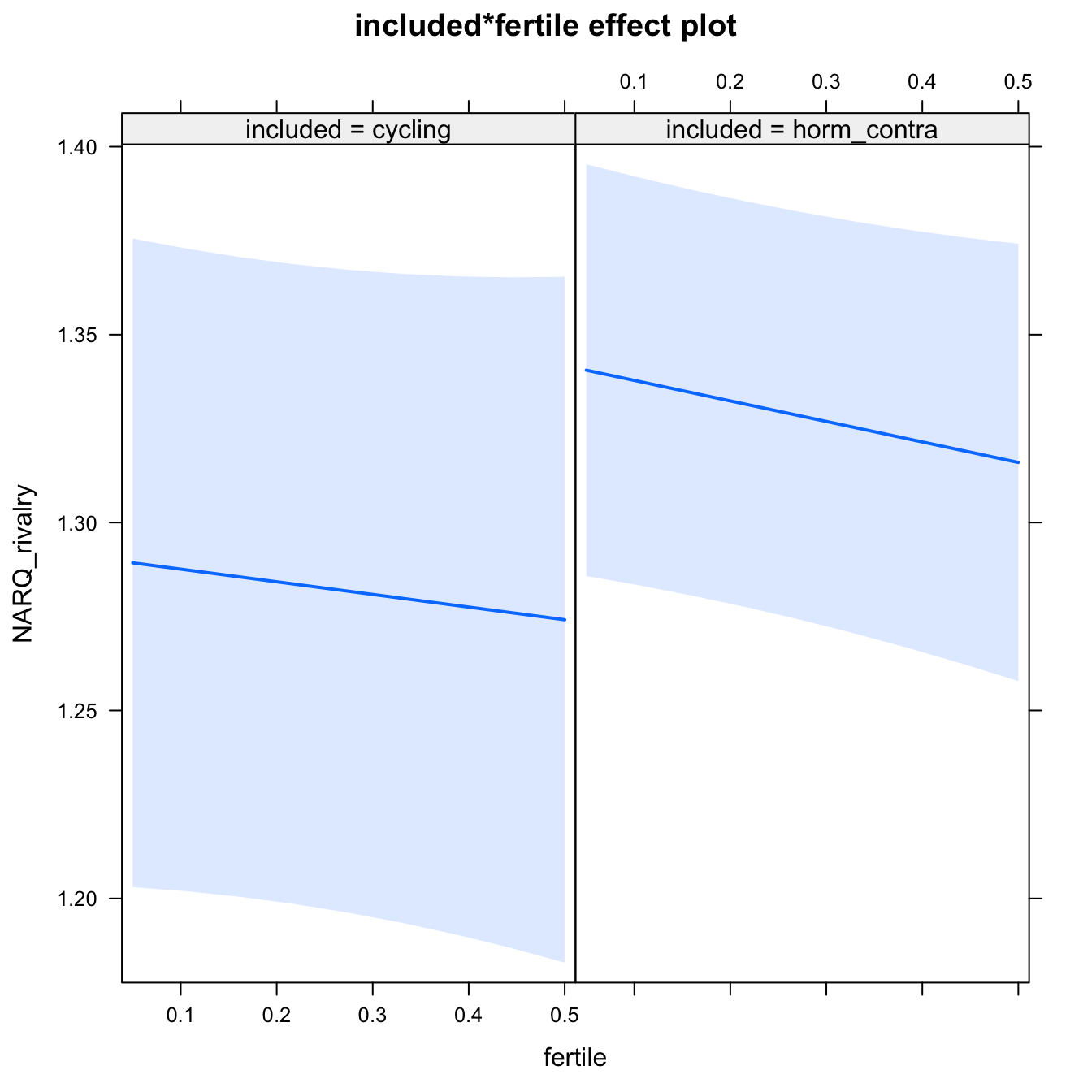
Diagnostics
model %>%
plot_outcome(diary) %>%
print_diagnostics()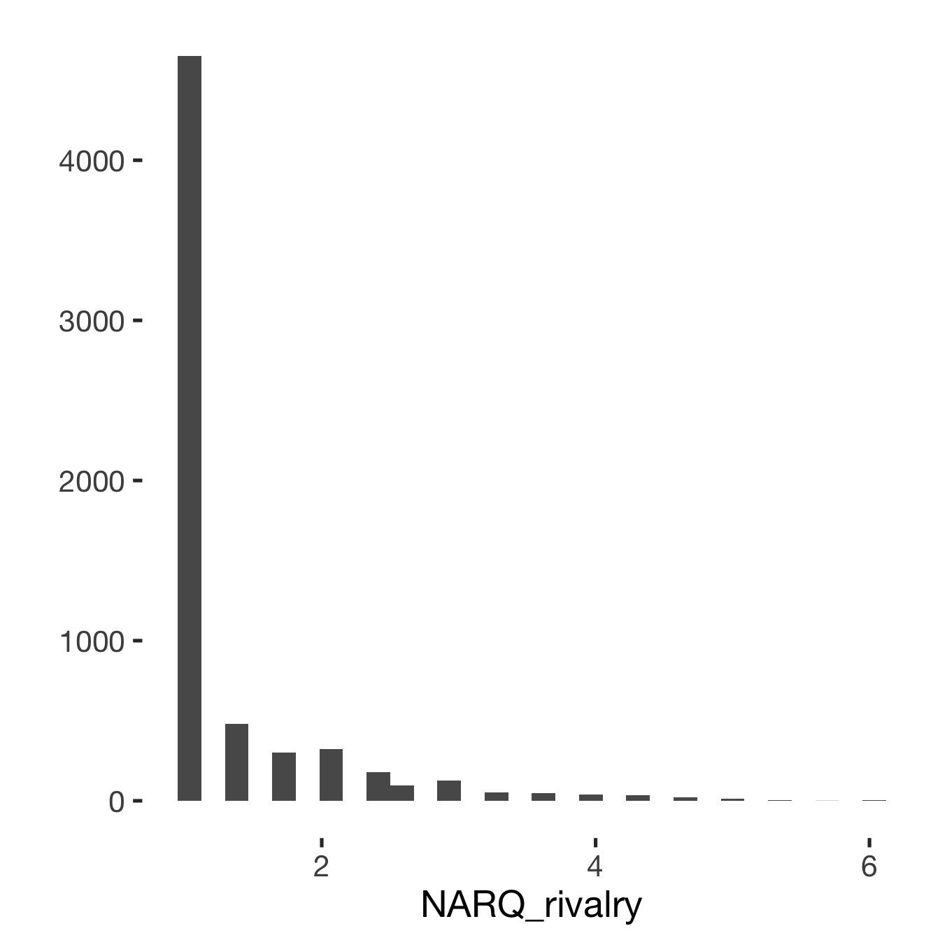
## Error in qqnorm.default(resid(obj)): y is empty or has only NAs
Adjusting for self esteem
model %>%
adjust_for_self_esteem(diary)##
##
## ```
## Linear mixed model fit by REML. t-tests use Satterthwaite's method ['lmerModLmerTest']
## Formula: form
## Data: diary
##
## REML criterion at convergence: 10135
##
## Scaled residuals:
## Min 1Q Median 3Q Max
## -4.680 -0.330 -0.102 0.002 9.534
##
## Random effects:
## Groups Name Variance Std.Dev.
## person (Intercept) 0.242 0.492
## Residual 0.234 0.483
## Number of obs: 6378, groups: person, 493
##
## Fixed effects:
## Estimate Std. Error df t value Pr(>|t|)
## (Intercept) 1.41995 0.05366 1074.19798 26.46 < 2e-16 ***
## includedhorm_contra 0.04962 0.05257 543.87630 0.94 0.35
## fertile -0.03276 0.05413 5936.98805 -0.61 0.55
## self_esteem_1 -0.03004 0.00703 6343.85374 -4.27 0.00002 ***
## includedhorm_contra:fertile -0.01954 0.06481 5940.55217 -0.30 0.76
## ---
## Signif. codes: 0 '***' 0.001 '**' 0.01 '*' 0.05 '.' 0.1 ' ' 1
##
## Correlation of Fixed Effects:
## (Intr) incld_ fertil slf__1
## inclddhrm_c -0.705
## fertile -0.188 0.194
## self_estm_1 -0.563 0.012 -0.004
## inclddhrm_: 0.161 -0.232 -0.835 -0.005
##
## ```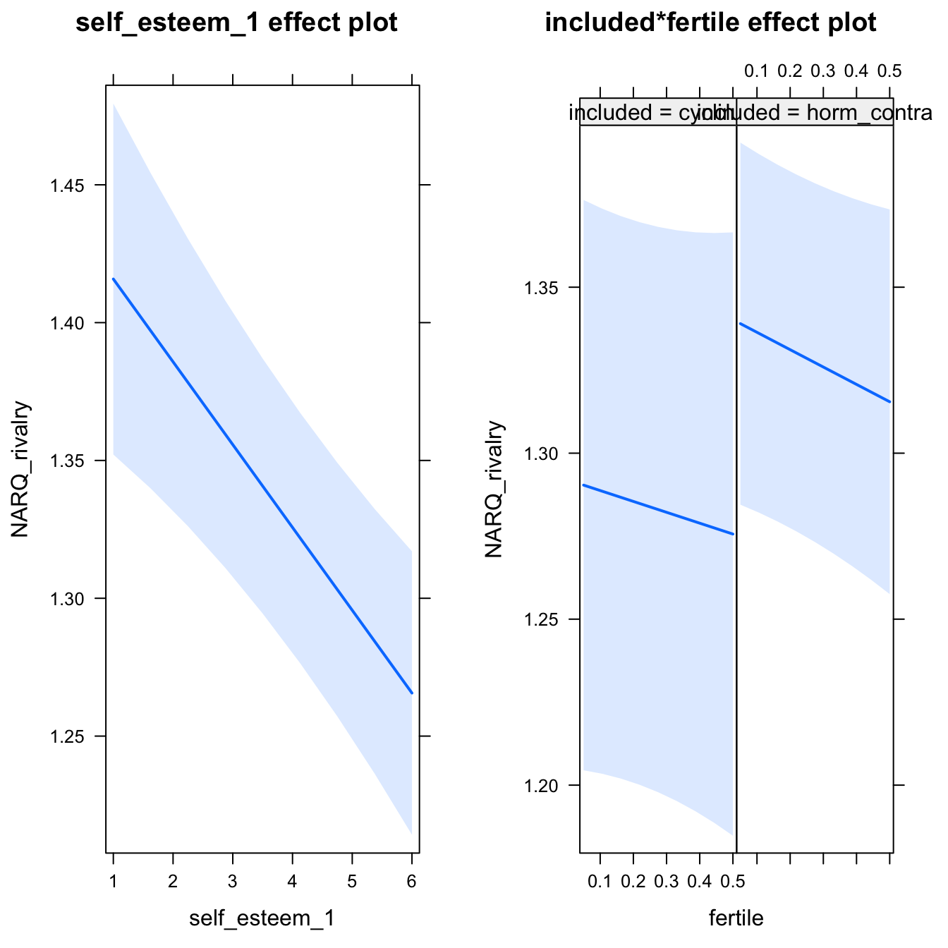
Broad window
outcome = names(model@frame)[1]
broad_models[[outcome]] <<- model %>%
switch_window_to_broad(diary)Linear mixed model fit by REML. t-tests use Satterthwaite's method ['lmerModLmerTest']
Formula: form
Data: diary2
REML criterion at convergence: 12384
Scaled residuals:
Min 1Q Median 3Q Max
-4.660 -0.345 -0.100 -0.025 9.395
Random effects:
Groups Name Variance Std.Dev.
person (Intercept) 0.231 0.480
Residual 0.244 0.494
Number of obs: 7740, groups: person, 493
Fixed effects:
Estimate Std. Error df t value Pr(>|t|)
(Intercept) 1.28978 0.04358 564.94519 29.60 <2e-16 ***
includedhorm_contra 0.05086 0.05164 568.00906 0.99 0.33
fertile 0.00501 0.05542 7319.07785 0.09 0.93
includedhorm_contra:fertile -0.04745 0.06621 7324.42347 -0.72 0.47
---
Signif. codes: 0 '***' 0.001 '**' 0.01 '*' 0.05 '.' 0.1 ' ' 1
Correlation of Fixed Effects:
(Intr) incld_ fertil
inclddhrm_c -0.844
fertile -0.267 0.225
inclddhrm_: 0.223 -0.270 -0.837
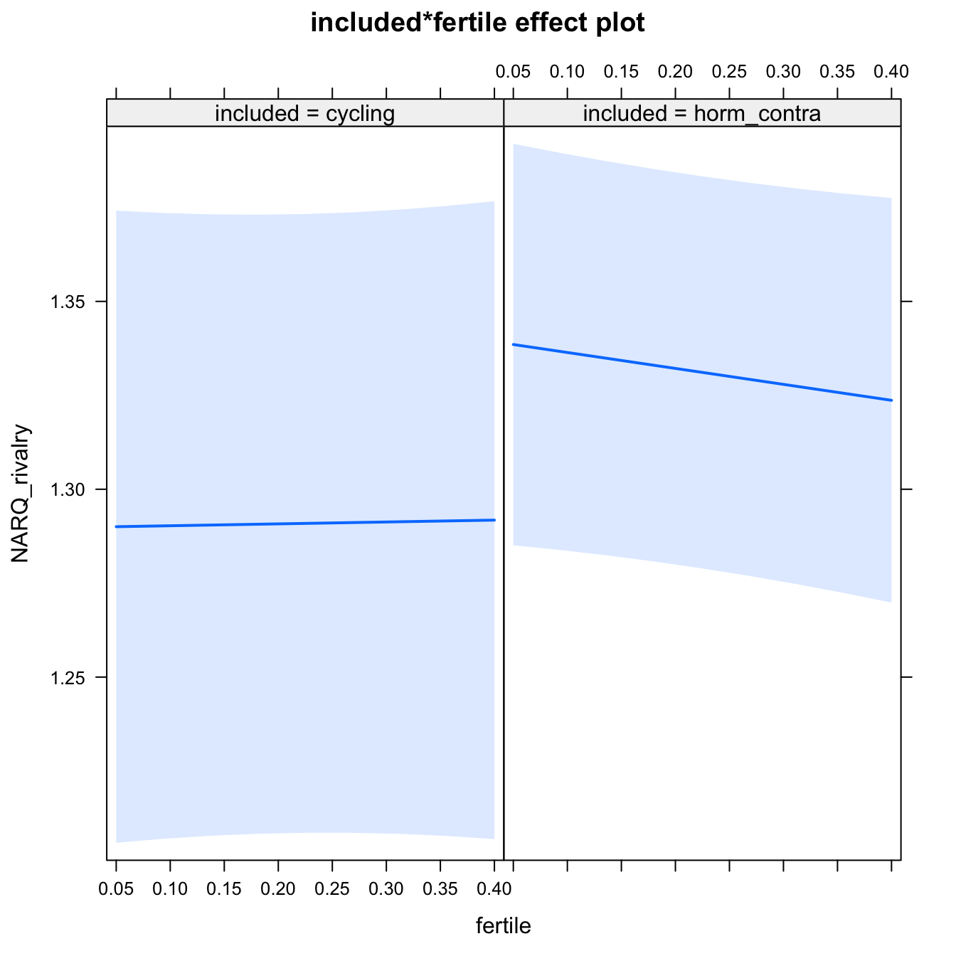
Diagnostics
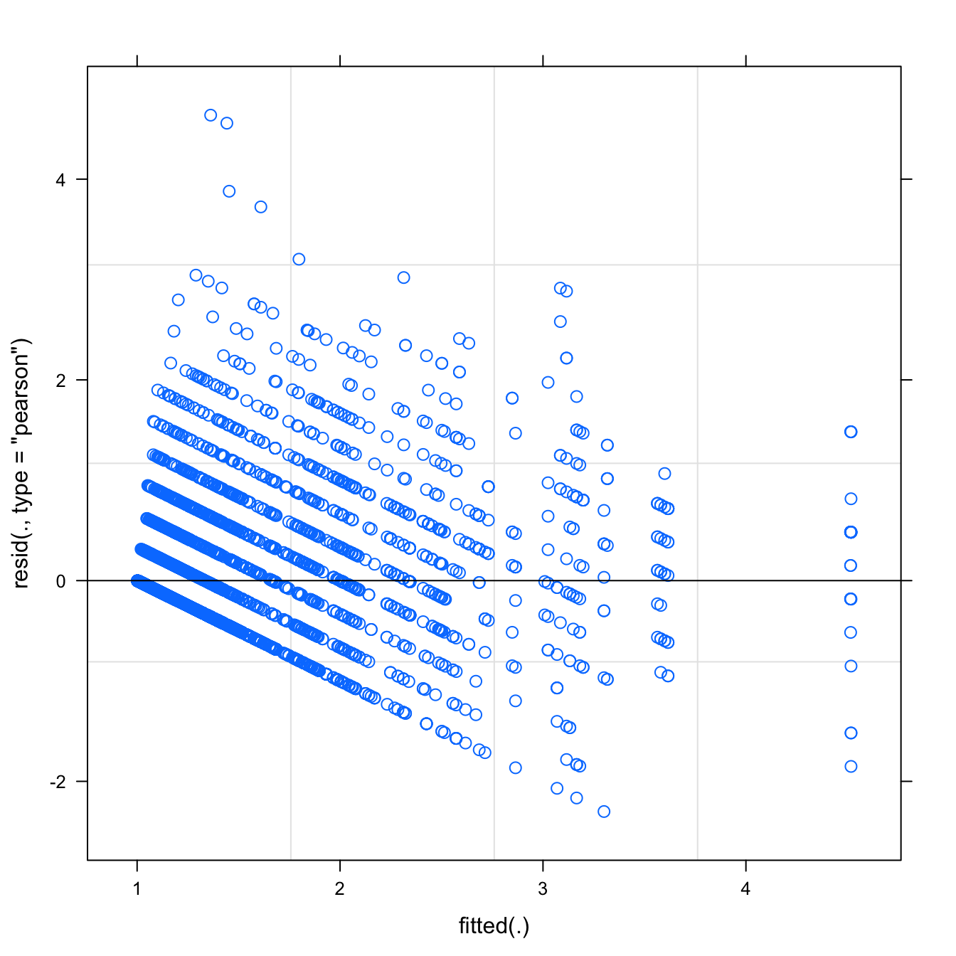
## Warning: 'sjp.lmer' is deprecated.
## Use 'plot_model' instead.
## See help("Deprecated")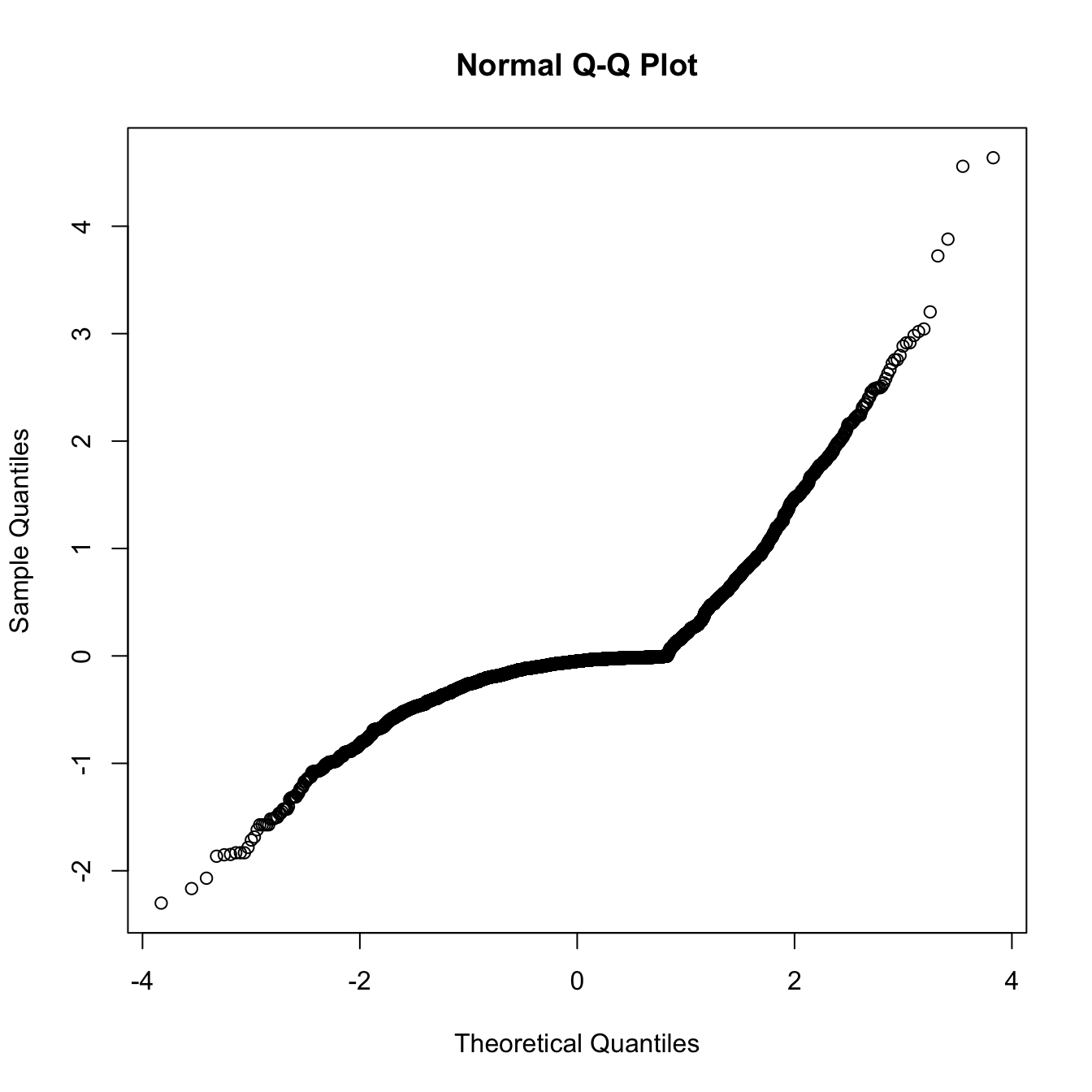
## Warning: 'sjp.lmer' is deprecated.
## Use 'plot_model' instead.
## See help("Deprecated")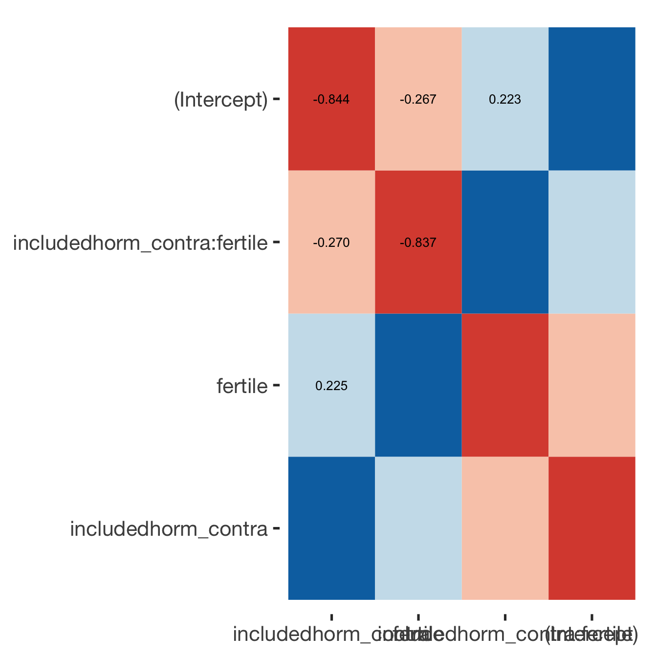
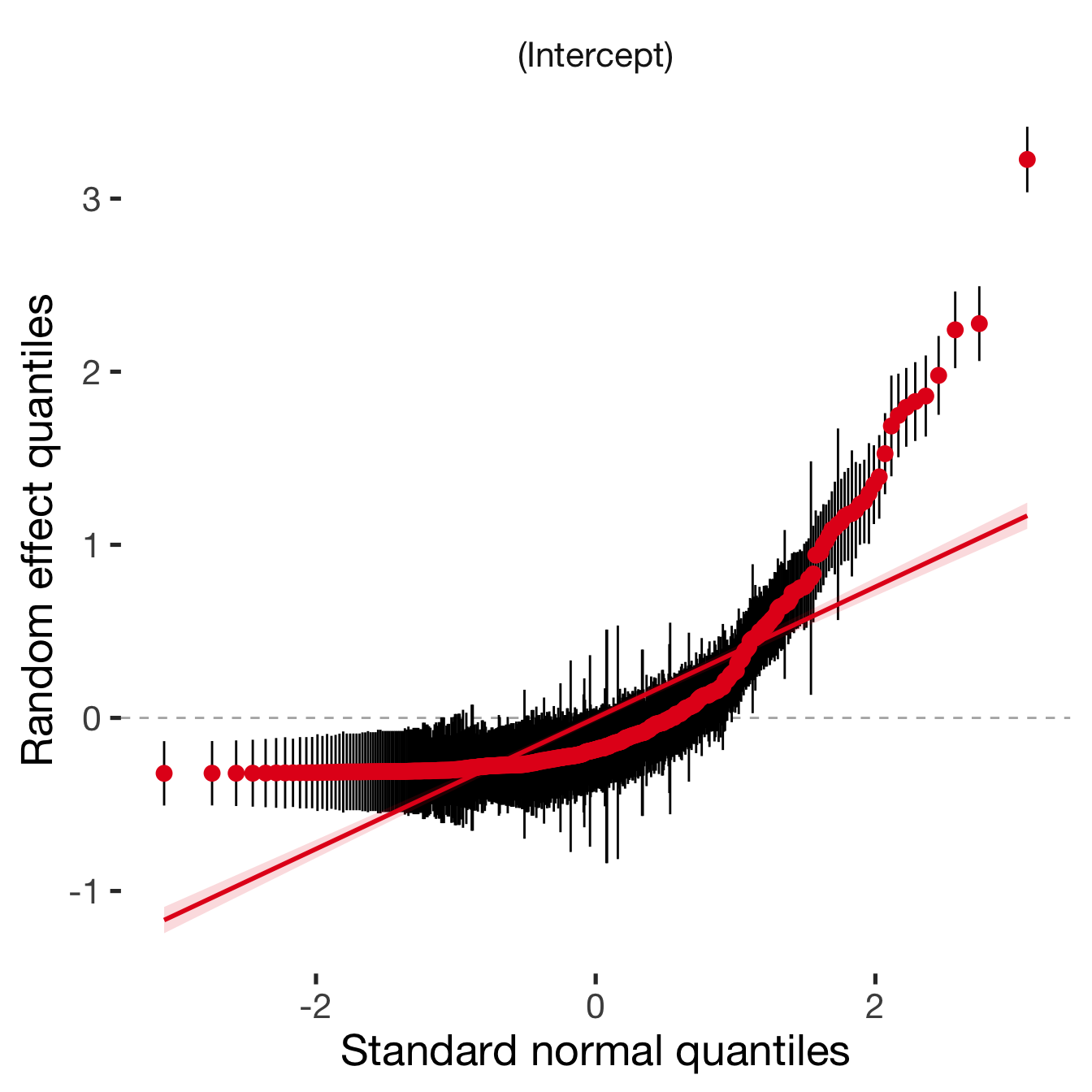
Adjusting for self esteem
broad_models[[outcome]] %>%
adjust_for_self_esteem(diary2)##
##
## ```
## Linear mixed model fit by REML. t-tests use Satterthwaite's method ['lmerModLmerTest']
## Formula: form
## Data: diary
##
## REML criterion at convergence: 12372
##
## Scaled residuals:
## Min 1Q Median 3Q Max
## -4.643 -0.345 -0.107 -0.002 9.519
##
## Random effects:
## Groups Name Variance Std.Dev.
## person (Intercept) 0.229 0.478
## Residual 0.243 0.493
## Number of obs: 7740, groups: person, 493
##
## Fixed effects:
## Estimate Std. Error df t value Pr(>|t|)
## (Intercept) 1.41174 0.05154 1058.63245 27.39 < 2e-16 ***
## includedhorm_contra 0.04839 0.05146 568.50923 0.94 0.35
## fertile 0.00737 0.05537 7318.60595 0.13 0.89
## self_esteem_1 -0.02840 0.00647 7715.32331 -4.39 0.000011 ***
## includedhorm_contra:fertile -0.04682 0.06614 7323.82764 -0.71 0.48
## ---
## Signif. codes: 0 '***' 0.001 '**' 0.01 '*' 0.05 '.' 0.1 ' ' 1
##
## Correlation of Fixed Effects:
## (Intr) incld_ fertil slf__1
## inclddhrm_c -0.717
## fertile -0.220 0.225
## self_estm_1 -0.539 0.011 -0.010
## inclddhrm_: 0.190 -0.271 -0.837 -0.002
##
## ```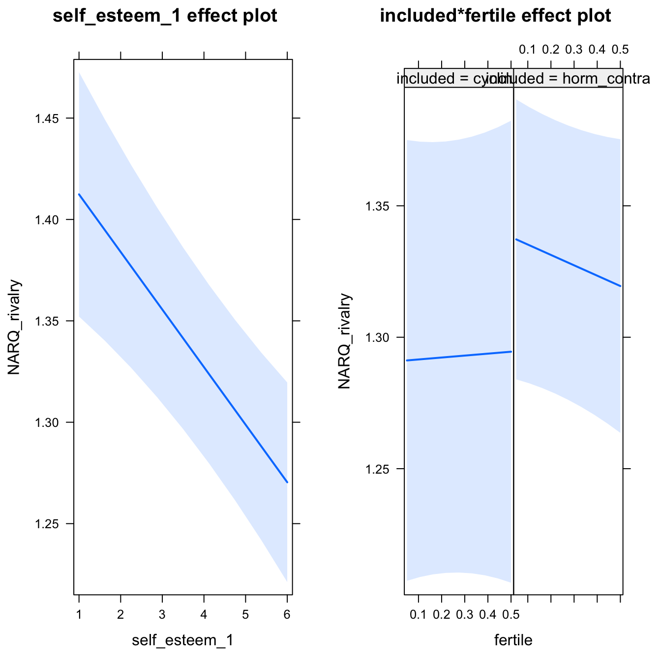
bla = 2H3.1. Self esteem
self_esteem_1 = lmer(self_esteem_1 ~ included * fertile + ( 1 | person), data = diary)
summary(self_esteem_1)## Linear mixed model fit by REML. t-tests use Satterthwaite's method ['lmerModLmerTest']
## Formula: self_esteem_1 ~ included * fertile + (1 | person)
## Data: diary
##
## REML criterion at convergence: 17475
##
## Scaled residuals:
## Min 1Q Median 3Q Max
## -4.944 -0.501 0.101 0.620 3.631
##
## Random effects:
## Groups Name Variance Std.Dev.
## person (Intercept) 0.573 0.757
## Residual 0.756 0.869
## Number of obs: 6379, groups: person, 493
##
## Fixed effects:
## Estimate Std. Error df t value Pr(>|t|)
## (Intercept) 4.2945 0.0698 561.8191 61.57 <2e-16 ***
## includedhorm_contra -0.0904 0.0827 565.4567 -1.09 0.27
## fertile 0.0281 0.0973 5957.3925 0.29 0.77
## includedhorm_contra:fertile 0.0471 0.1165 5962.1515 0.40 0.69
## ---
## Signif. codes: 0 '***' 0.001 '**' 0.01 '*' 0.05 '.' 0.1 ' ' 1
##
## Correlation of Fixed Effects:
## (Intr) incld_ fertil
## inclddhrm_c -0.844
## fertile -0.263 0.222
## inclddhrm_: 0.219 -0.265 -0.835plot(allEffects(self_esteem_1))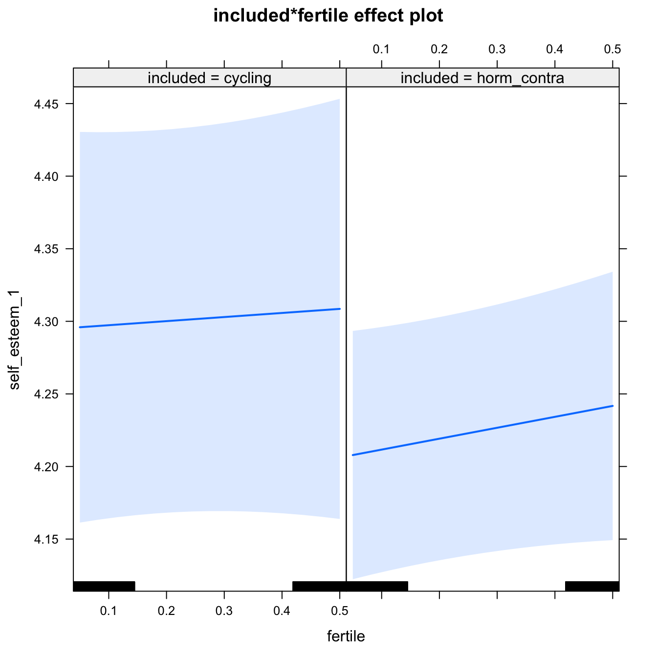
Coefficient plot
library(broom)
library(broom.mixed)
collect = . %>% lapply(FUN = tidy, conf.int = TRUE) %>%
bind_rows(.id = "outcome") %>%
mutate(
outcome = recode(str_replace_all(str_replace_all(outcome, "_", " "), " pair", "-pair"),
"desirability 1" = "self-perceived desirability",
"NARQ admiration" = "narcissistic admiration",
"NARQ rivalry" = "narcissistic rivalry",
"extra-pair" = "extra-pair desire & behaviour",
"had sexual intercourse" = "sexual intercourse"),
outcome = factor(outcome),
term = recode(term, "includedhorm_contra" = "HC user",
"includedhorm_contra:fertile" = "HC user x fertile",
"self_esteem_1" = "self esteem"),
term = factor(term),
group = factor(group))
coefs = bind_rows(`Narrow window BC` = models %>% collect, `Broad window BC` = broad_models %>% collect, .id = "window") %>% mutate(window = factor(window))
coefs %>% filter(term %contains% "fertile") %>%
ggplot(., aes(x = outcome, y = estimate, ymax = conf.high, ymin = conf.low, colour = term)) +
geom_hline(yintercept = 0, linetype = "dotted", color = "gray70") +
geom_text(aes(label = form(estimate), y = estimate), vjust = -0.7,position = position_dodge(width = 0.6)) +
geom_pointrange( position = position_dodge(width = 0.6), size = 1) +
scale_color_manual("Contraception status", values = c("HC user x fertile"="black","fertile" = "red"), labels = c("HC user x fertile"="hormonally\ncontracepting","fertile" = "fertile"), guide = F) +
coord_flip() +
facet_wrap(~ window)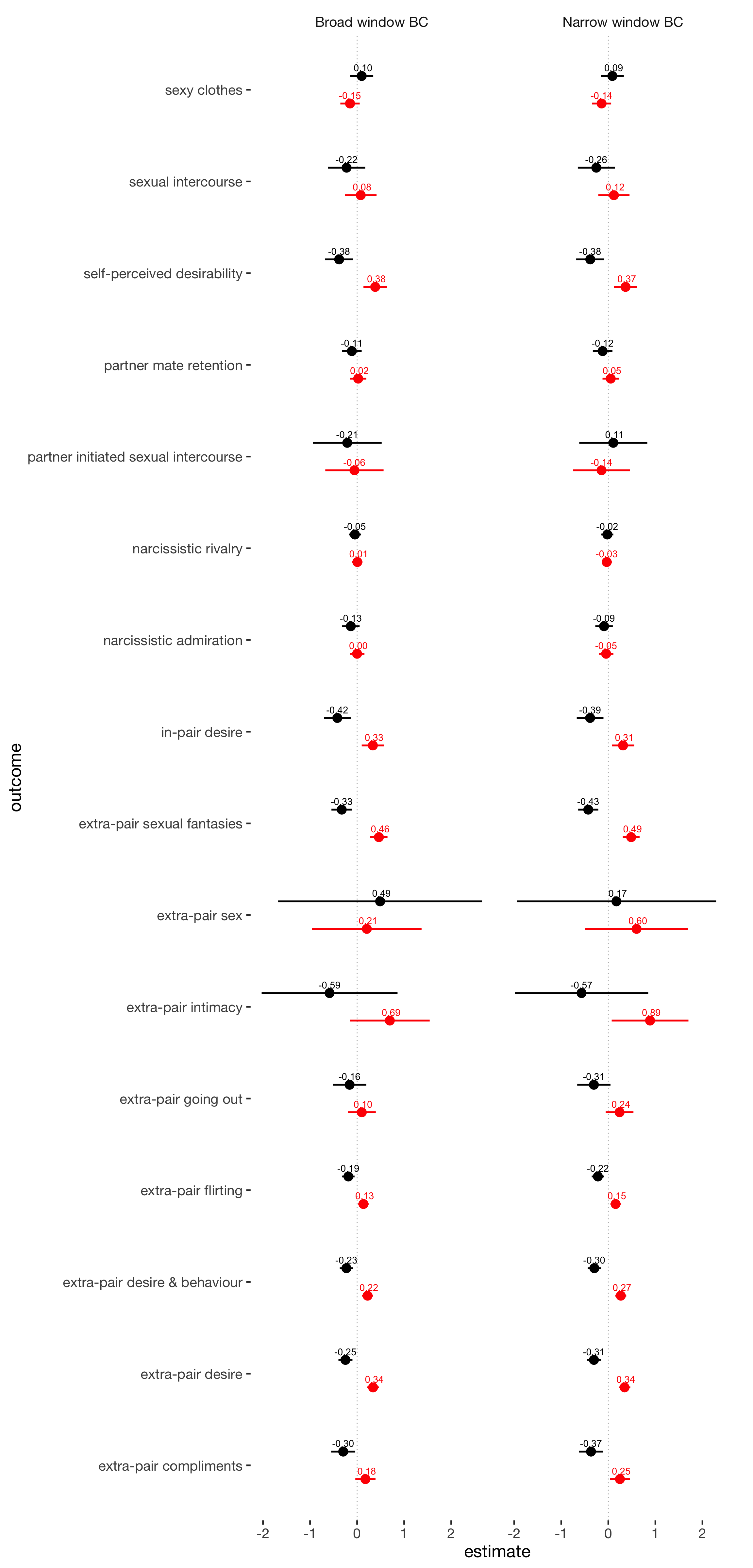
Table
Complete interactive table
library(DT)
coefs %>%
datatable(rownames = FALSE, filter = "top", extensions = 'Buttons', options = list(
dom = 'Bfrtip',
buttons = c('copy', 'csv', 'excel', 'pdf', 'print'),
pageLength = 20
)) %>%
formatRound(c("estimate", "std.error", "statistic", "conf.low", "conf.high"), 2) %>%
formatRound(c("p.value"), 4)Table for paper
coefs %>%
filter(!term %starts_with% "sd_", window %contains% "Narrow") %>%
mutate(
p.value_apa = pvalues(p.value),
estimate = paste0(
form(estimate), "±", form(std.error), "\\\n_p_ ",
p.value_apa
# "<sup>", if_else(p.value < 0.001, "**",
# if_else(p.value < 0.01, "*", "")), "</sup>"
)
) %>%
select(outcome, term, estimate) %>%
spread(term, estimate) %>%
pander(keep.line.breaks = TRUE)| outcome | (Intercept) | fertile | HC user | HC user x fertile |
|---|---|---|---|---|
| extra-pair compliments | 2.37±0.08 p < .001 |
0.25±0.11 p = .023 |
-0.11±0.10 p = .267 |
-0.37±0.13 p = .005 |
| extra-pair desire | 1.65±0.05 p < .001 |
0.34±0.06 p < .001 |
-0.13±0.06 p = .047 |
-0.31±0.07 p < .001 |
| extra-pair desire & behaviour | 1.75±0.05 p < .001 |
0.27±0.06 p < .001 |
-0.05±0.06 p = .373 |
-0.30±0.07 p < .001 |
| extra-pair flirting | 1.36±0.04 p < .001 |
0.15±0.06 p = .006 |
-0.09±0.05 p = .078 |
-0.22±0.07 p < .001 |
| extra-pair going out | 1.99±0.09 p < .001 |
0.24±0.15 p = .113 |
0.24±0.10 p = .019 |
-0.31±0.18 p = .088 |
| extra-pair intimacy | -4.47±0.30 p < .001 |
0.89±0.42 p = .033 |
-0.22±0.37 p = .554 |
-0.57±0.72 p = .431 |
| extra-pair sex | -4.60±0.39 p < .001 |
0.60±0.56 p = .282 |
-0.44±0.57 p = .444 |
0.17±1.08 p = .873 |
| extra-pair sexual fantasies | 1.50±0.06 p < .001 |
0.49±0.09 p < .001 |
-0.19±0.08 p = .012 |
-0.43±0.11 p < .001 |
| in-pair desire | 3.48±0.08 p < .001 |
0.31±0.12 p = .010 |
0.24±0.09 p = .010 |
-0.39±0.14 p = .008 |
| narcissistic admiration | 2.69±0.10 p < .001 |
-0.05±0.08 p = .551 |
-0.14±0.11 p = .214 |
-0.09±0.09 p = .335 |
| narcissistic rivalry | 1.29±0.04 p < .001 |
-0.03±0.05 p = .535 |
0.05±0.05 p = .322 |
-0.02±0.06 p = .747 |
| partner initiated sexual intercourse | 0.26±0.09 p = .005 |
-0.14±0.31 p = .642 |
0.12±0.11 p = .276 |
0.11±0.37 p = .775 |
| partner mate retention | 2.86±0.07 p < .001 |
0.05±0.09 p = .569 |
0.00±0.08 p = .954 |
-0.12±0.11 p = .255 |
| self-perceived desirability | 3.72±0.08 p < .001 |
0.37±0.13 p = .004 |
-0.07±0.09 p = .477 |
-0.38±0.15 p = .012 |
| sexual intercourse | -0.98±0.07 p < .001 |
0.12±0.17 p = .483 |
0.17±0.08 p = .026 |
-0.26±0.20 p = .203 |
| sexy clothes | 3.16±0.07 p < .001 |
-0.14±0.10 p = .169 |
0.02±0.08 p = .831 |
0.09±0.12 p = .492 |
# datatable(rownames = FALSE, filter = "top", extensions = 'Buttons', options = list(
# dom = 'Bfrtip',
# buttons = c('copy', 'csv', 'excel', 'pdf', 'print'),
# pageLength = 40
# ), escape = FALSE)Benjamini-Hochberg
Narrow window
ps_named = coefs %>% filter(
term == "fertile", window == "Narrow window BC"
) %>% select(outcome, p.value)
ps = ps_named$p.value
names(ps) = ps_named$outcome
p.adj = p.adjust(ps, method = "BH")
data.frame(outcome = ps_named$outcome, p.value.adj = p.adj) %>% arrange(p.value.adj) %>% pander()| outcome | p.value.adj |
|---|---|
| extra-pair desire | 0.000000543 |
| extra-pair sexual fantasies | 0.0000008211 |
| extra-pair desire & behaviour | 0.00004478 |
| self-perceived desirability | 0.01606 |
| extra-pair flirting | 0.0184 |
| in-pair desire | 0.02655 |
| extra-pair compliments | 0.05361 |
| extra-pair intimacy | 0.06629 |
| extra-pair going out | 0.2006 |
| sexy clothes | 0.2704 |
| extra-pair sex | 0.4108 |
| sexual intercourse | 0.6067 |
| partner mate retention | 0.6067 |
| narcissistic admiration | 0.6067 |
| narcissistic rivalry | 0.6067 |
| partner initiated sexual intercourse | 0.6418 |
Broad window
ps_named = coefs %>% filter(
term == "fertile", window == "Broad window BC"
) %>% select(outcome, p.value)
ps = ps_named$p.value
names(ps) = ps_named$outcome
p.adj = p.adjust(ps, method = "BH")
data.frame(outcome = ps_named$outcome, p.value.adj = p.adj) %>% arrange(p.value.adj) %>% pander()| outcome | p.value.adj |
|---|---|
| extra-pair desire | 0.000001682 |
| extra-pair sexual fantasies | 0.000005784 |
| extra-pair desire & behaviour | 0.001243 |
| self-perceived desirability | 0.0102 |
| in-pair desire | 0.01859 |
| extra-pair flirting | 0.04519 |
| extra-pair compliments | 0.2162 |
| extra-pair intimacy | 0.2162 |
| sexy clothes | 0.2664 |
| extra-pair going out | 0.8223 |
| sexual intercourse | 0.9519 |
| extra-pair sex | 0.9722 |
| partner initiated sexual intercourse | 0.9783 |
| partner mate retention | 0.9783 |
| narcissistic rivalry | 0.9898 |
| narcissistic admiration | 0.9901 |
saveRDS(models, file = "models_prereg.rds")