Robustness checks of ovulatory changes
Cycling women (not on hormonal birth control)
Women on hormonal birth control
Load data
# cd /usr/users/rarslan/relationship_dynamics/ && bsub -q mpi -W 48:00 -n 20 -R span[hosts=1] R -e "filebase = '3_fertility_robustness'; x = rmarkdown::render(paste0('3_fertility_robustness','.Rmd'), run_pandoc = FALSE, clean = FALSE); save(x, file = 'rob.rda'); cat(readLines(paste0(filebase,'.utf8.md')), sep = '\n')"
library(knitr)
opts_chunk$set(fig.width = 8, fig.height = 8, cache = T, warning = T, message = F, cache = F)
source("0_helpers.R")
load("full_data.rdata")
diary = diary %>%
mutate(
included = included_all,
fertile = if_else(is.na(prc_stirn_b_squished), prc_stirn_b_backward_inferred, prc_stirn_b_squished),
contraceptive_methods = factor(contraceptive_method, levels =
c("barrier_or_abstinence", "fertility_awareness", "none", "hormonal")),
relationship_status_clean = factor(relationship_status_clean),
cohabitation = factor(cohabitation),
certainty_menstruation = as.numeric(as.character(certainty_menstruation)),
partner_st_vs_lt = partner_attractiveness_shortterm - partner_attractiveness_longterm
) %>% group_by(person) %>%
mutate(
fertile_mean = mean(fertile, na.rm = T)
)
opts_chunk$set(warning = F)
library(Cairo)
opts_chunk$set(dev = "CairoPNG")
diary$age_group = cut(diary$age,c(18,20,25,30,35,70), include.lowest = T)models = list()
do_model = function(model, diary) {
outcome = names(model@frame)[1]
outcome_label = recode(str_replace_all(str_replace_all(str_replace_all(outcome, "_", " "), " pair", "-pair"), " 1", ""),
"desirability" = "self-perceived desirability",
"NARQ admiration" = "narcissistic admiration",
"NARQ rivalry" = "narcissistic rivalry",
"extra-pair" = "extra-pair desire & behaviour",
"had sexual intercourse" = "sexual intercourse")
model = calculate_effects(model)
options = list(fig.path = paste0(knitr::opts_chunk$get("fig.path"), outcome, "-"),
cache.path = paste0(knitr::opts_chunk$get("cache.path"), outcome, "-"))
asis_knit_child("_robustness_model.Rmd", options = options)
}
do_moderators = function(model, diary) {
asis_knit_child("_moderators.Rmd")
}models$extra_pair = lmer(extra_pair ~ included * (menstruation + fertile) + fertile_mean + ( 1 | person), data = diary)
models$desirability_1 = lmer(desirability_1 ~ included * (menstruation + fertile) + fertile_mean + ( 1 | person), data = diary)
models$extra_pair_intimacy = glmer(extra_pair_intimacy ~ included * (menstruation + fertile) + fertile_mean + ( 1 | person), data = diary, family = binomial(link = "probit"))
models$extra_pair_sex = glmer(extra_pair_sex ~ included * (menstruation + fertile) + fertile_mean + ( 1 | person), data = diary, family = binomial(link = "probit"))
models$in_pair_desire = lmer(in_pair_desire ~ included * (menstruation + fertile) + fertile_mean + ( 1 | person), data = diary)
models$had_petting = glmer(had_petting ~ included * (menstruation + fertile) + fertile_mean + ( 1 | person), data = diary, family = binomial(link = "probit"))
models$had_sexual_intercourse = glmer(had_sexual_intercourse ~ included * (menstruation + fertile) + fertile_mean + ( 1 | person), data = diary, family = binomial(link = "probit"))
models$partner_initiated_sexual_intercourse = glmer(partner_initiated_sexual_intercourse ~ included * (menstruation + fertile) + fertile_mean + ( 1 | person), data = diary, family = binomial(link = "probit"))
models$sexual_intercourse_satisfaction = lmer(sexual_intercourse_satisfaction ~ included * (menstruation + fertile) + fertile_mean + ( 1 | person), data = diary)
models$spent_night_with_partner = glmer(spent_night_with_partner ~ included * (menstruation + fertile) + fertile_mean + ( 1 | person), data = diary, family = binomial(link = "probit"))
models$partner_mate_retention = lmer(partner_mate_retention ~ included * (menstruation + fertile) + fertile_mean + ( 1 | person), data = diary)
models$female_mate_retention = lmer(female_mate_retention ~ included * (menstruation + fertile) + fertile_mean + ( 1 | person), data = diary)
models$sexy_clothes = lmer(sexy_clothes ~ included * (menstruation + fertile) + fertile_mean + ( 1 | person), data = diary)
models$showy_clothes = lmer(showy_clothes ~ included * (menstruation + fertile) + fertile_mean + ( 1 | person), data = diary)
models$male_attention_1 = lmer(male_attention_1 ~ included * (menstruation + fertile) + fertile_mean + ( 1 | person), data = diary)
models$in_pair_public_intimacy = glmer(in_pair_public_intimacy ~ included * (menstruation + fertile) + fertile_mean + ( 1 | person), data = diary, family = binomial(link = "probit"))
models$NARQ_admiration = lmer(NARQ_admiration ~ included * (menstruation + fertile) + fertile_mean + ( 1 | person), data = diary)
models$NARQ_rivalry = lmer(NARQ_rivalry ~ included * (menstruation + fertile) + fertile_mean + ( 1 | person), data = diary)
models$self_esteem_1 = lmer(self_esteem_1 ~ included * (menstruation + fertile) + fertile_mean + ( 1 | person), data = diary)
models$female_jealousy = lmer(female_jealousy ~ included * (menstruation + fertile) + fertile_mean + ( 1 | person), data = diary)
models$relationship_satisfaction_1 = lmer(relationship_satisfaction_1 ~ included * (menstruation + fertile) + fertile_mean + ( 1 | person), data = diary)
models$communication_partner_1 = lmer(communication_partner_1 ~ included * (menstruation + fertile) + fertile_mean + ( 1 | person), data = diary)model_summaries = parallel::mclapply(models, FUN = do_model, diary = diary, mc.cores = 20)Extra-pair
model_summaries$extra_pairModel summary
Model summary
model %>%
  print_summary()
Linear mixed model fit by REML
t-tests use Satterthwaite approximations to degrees of freedom ['lmerMod']
Formula: extra_pair ~ included * (menstruation + fertile) + fertile_mean + (1 | person)
Data: diary
REML criterion at convergence: 48549
Scaled residuals:
Min 1Q Median 3Q Max
-4.286 -0.557 -0.148 0.405 8.007
Random effects:
Groups Name Variance Std.Dev.
person (Intercept) 0.311 0.558
Residual 0.320 0.566
Number of obs: 26680, groups: person, 1054
Fixed effects:
Estimate Std. Error df t value Pr(>|t|)
(Intercept) 1.8341 0.0470 1311.0000 39.06 < 2e-16 ***
includedhorm_contra -0.1181 0.0386 1259.0000 -3.06 0.0022 **
menstruationpre -0.0905 0.0173 25899.0000 -5.23 0.00000017 ***
menstruationyes -0.0713 0.0163 25993.0000 -4.37 0.00001240 ***
fertile 0.1730 0.0349 25894.0000 4.96 0.00000072 ***
fertile_mean -0.0558 0.2140 1421.0000 -0.26 0.7945
includedhorm_contra:menstruationpre 0.0691 0.0222 25895.0000 3.11 0.0019 **
includedhorm_contra:menstruationyes 0.0858 0.0214 25974.0000 4.02 0.00005958 ***
includedhorm_contra:fertile -0.1742 0.0442 25999.0000 -3.94 0.00008279 ***
---
Signif. codes: 0 '***' 0.001 '**' 0.01 '*' 0.05 '.' 0.1 ' ' 1
Correlation of Fixed Effects:
(Intr) incld_ mnstrtnp mnstrtny fertil frtl_m inclddhrm_cntr:mnstrtnp
inclddhrm_c -0.474
menstrutnpr -0.140 0.179
menstrutnys -0.138 0.173 0.398
fertile -0.135 0.222 0.467 0.385
fertile_men -0.772 -0.024 -0.008 -0.005 -0.059
inclddhrm_cntr:mnstrtnp 0.116 -0.224 -0.779 -0.310 -0.363 -0.003
inclddhrm_cntr:mnstrtny 0.110 -0.212 -0.304 -0.763 -0.293 -0.003 0.384
inclddhrm_cntr:f 0.135 -0.280 -0.368 -0.303 -0.787 0.010 0.467
inclddhrm_cntr:mnstrtny
inclddhrm_c
menstrutnpr
menstrutnys
fertile
fertile_men
inclddhrm_cntr:mnstrtnp
inclddhrm_cntr:mnstrtny
inclddhrm_cntr:f 0.382
Effect size standardised by residual variance (\(\frac{b}{ SD_{residual} }\)): 0.31 [0.18;0.43].
Marginal effect plots
model %>%
  plot_all_effects()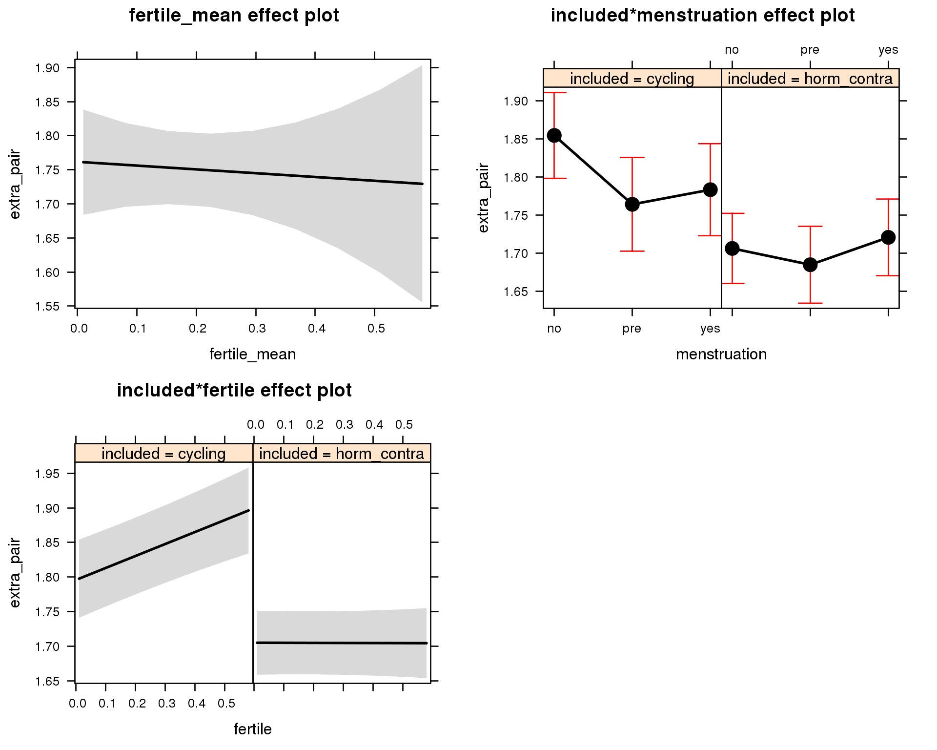
Outcome distribution
model %>%
  plot_outcome(diary) + xlab(outcome_label)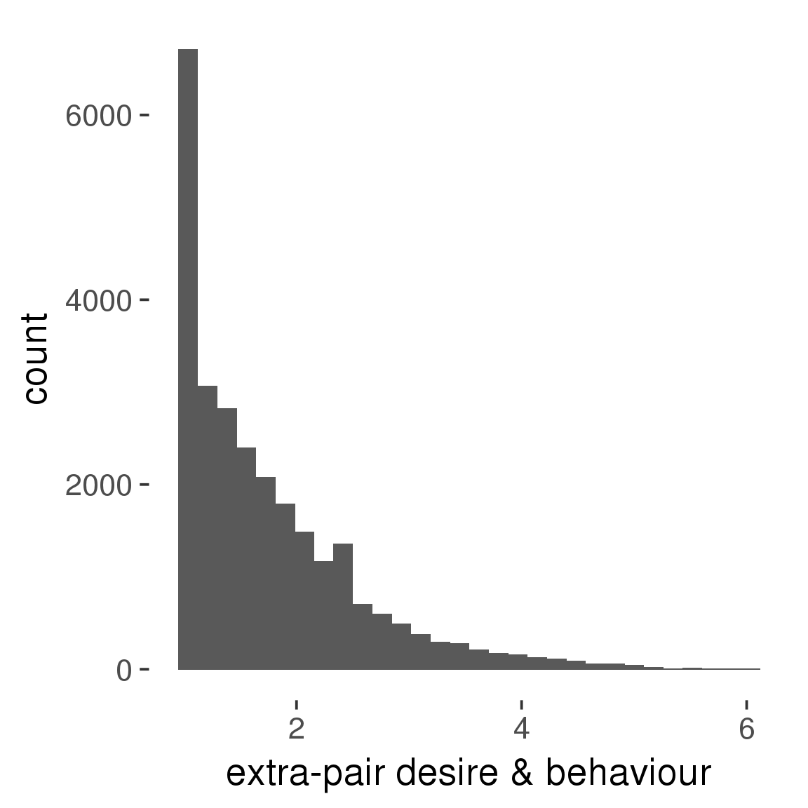
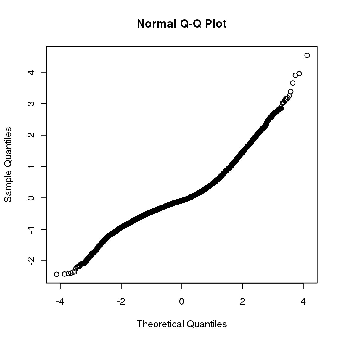
Diagnostics
model %>%
  print_diagnostics()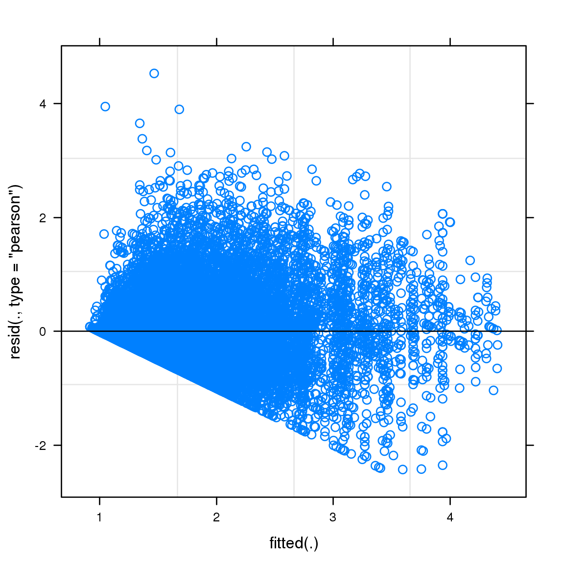


Curves
Here, we continuously plot the outcome over the course of the cycle. Because cycle lengths vary, we subset the data to cycles in a certain range. If the red curve traces the pink curve, our predictor accurately maps the relationship between fertile window probability and the outcome.
Cycle lengths from 21 to 36
Backward-counted
model %>%
  plot_curve(diary %>% filter(minimum_cycle_length_diary <= 36, minimum_cycle_length_diary > 20) %>% mutate(fertile=prc_stirn_b))
outcome = names(model@frame)[1]
outcome_label = recode(str_replace_all(str_replace_all(str_replace_all(outcome, "_", " "), " pair", "-pair"), " 1", ""),
"desirability 1" = "self-perceived desirability",
"NARQ admiration" = "narcissistic admiration",
"NARQ rivalry" = "narcissistic rivalry",
"extra-pair" = "extra-pair desire & behaviour",
"had sexual intercourse" = "sexual intercourse")
library(ggplot2)
# form a subset and run the model without the hormonal contraception and the fertility predictors
tmp = diary %>%
filter(!is.na(fertile), !is.na(included),
RCD > -1 * minimum_cycle_length_diary, RCD > -40)
new_form = update.formula(formula(model), new = . ~ . - fertile * included)
tmp$residuals = residuals(update(model, new_form, data = tmp , na.action = na.exclude))
tmp = tmp %>%
filter(!is.na(RCD), !is.na(residuals))
rcd_min = min(tmp$RCD)
tmp$real = FALSE
tmp_before = tmp
tmp_before$RCD = tmp_before$RCD + min(tmp$RCD) - 1
tmp_after = tmp
tmp_after$RCD = tmp_after$RCD - min(tmp$RCD) + 1
tmp$real = TRUE
tmp = bind_rows(tmp_before %>% filter(RCD > rcd_min - 11), tmp, tmp_after %>% filter(RCD < 11))GAM smooth on residuals
Here, we partialled out menstruation and individual random effects, then superimposed estimated probability of being in the fertile window scaled to the range of the estimated means. To address the periodicity of the cycle, we prepended and appended ten days of the timeseries to the end and the beginning of the timeseries. We then estimated the GAM and cut off the appended subsets before plotting.
tryCatch({
  trend_plot = ggplot(tmp,aes(x = RCD, y = residuals, colour = included)) +
    stat_smooth(geom = 'smooth',size = 0.8, fill = "#9ECAE1", method = 'gam', formula = y ~ s(x))
}, error = function(e){cat_message(e, "danger")})

tryCatch({
  trend_data = ggplot_build(trend_plot)$data[[1]]
}, error = function(e){cat_message(e, "danger")})

trend_data$RCD = round(trend_data$x)
trend_data = left_join(trend_data, tmp %>% select(real, RCD,fertile) %>% unique(), by = "RCD")
trend_data %>%
  filter(real == TRUE) %>%
  mutate(superimposed = ( ( (fertile - 0.01)/0.58) * (max(y)-min(y) ) ) + min(y) ) ->
  trend_data


ggplot(trend_data) +
  geom_ribbon(aes(x = x, ymin = ymin, ymax = ymax,  fill = factor(group)), alpha = 0.2) +
  geom_line(aes(x = x, y = y, colour = factor(group)), size = 0.8, stat = "identity") +
  scale_x_continuous(caption_x) +
  geom_line(aes(x = x, y = superimposed), color = "#a83fbf", size = 1, linetype = 'dashed') +
  annotate("text",x = mean(trend_data$x),  y = max(trend_data$superimposed,na.rm=T) + 0.1, label = 'superimposed fertility peak', color = "#a83fbf") +
  scale_y_continuous(outcome_label) +
  ggtitle("GAM smooth, residuals") +
  scale_color_manual("Contraception status",values = c("2"="black","1"= "red"), labels = c("2"="hormonally\ncontracepting","1"="cycling"), guide = F) +
  scale_fill_manual("Contraception status",values = c("2"="black","1"= "red"), labels = c("2"="hormonally\ncontracepting","1"="cycling"), guide = F)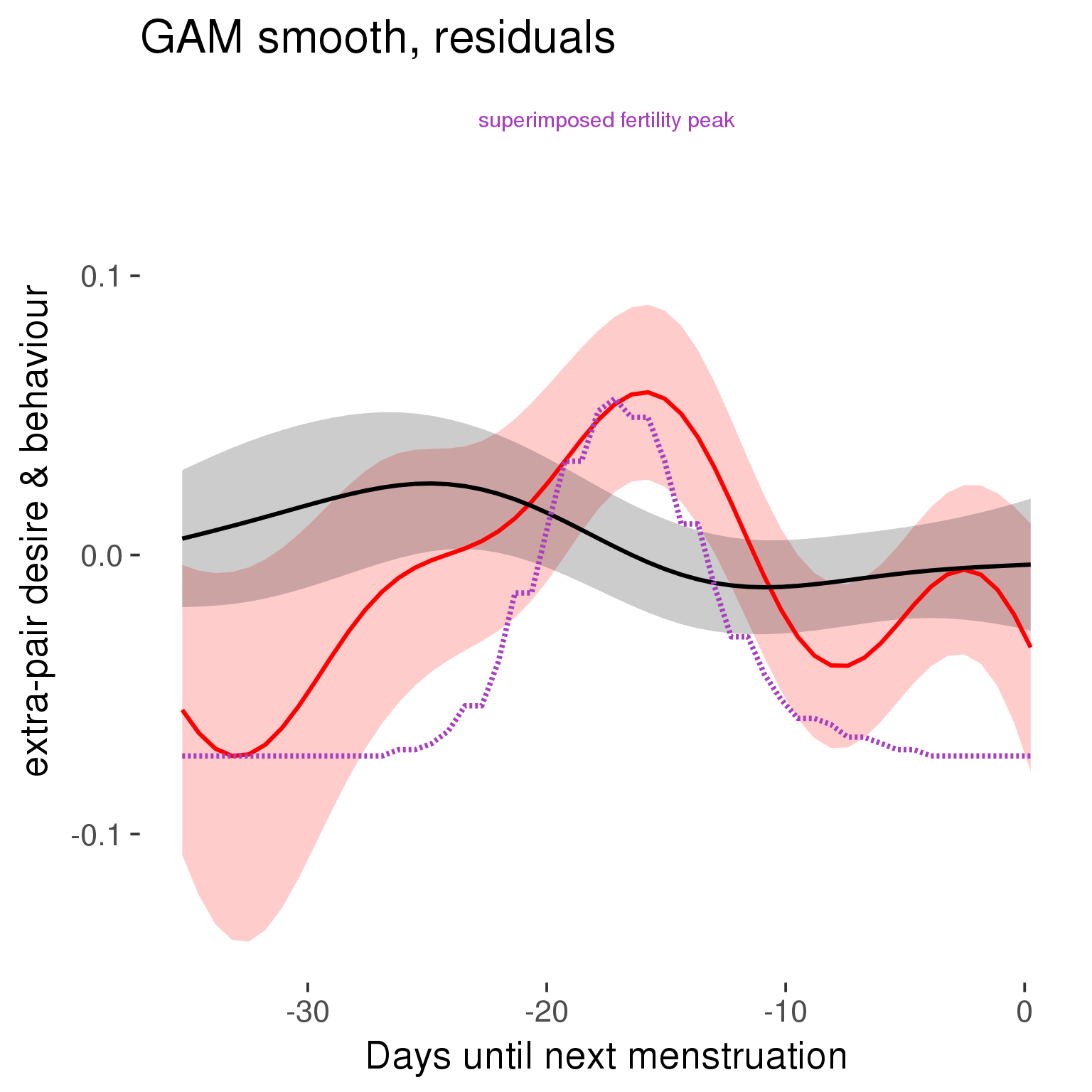
GAM smooth on raw data
As before, but without partialling anything out.
tryCatch({
  trend_plot = ggplot(tmp,aes_string(x = "RCD", y = outcome, colour = "included")) +
    stat_smooth(geom = 'smooth',size = 0.8, fill = "#9ECAE1", method = 'gam', formula = y ~ s(x))
}, error = function(e){cat_message(e, "danger")})

tryCatch({
  trend_data = ggplot_build(trend_plot)$data[[1]]
}, error = function(e){cat_message(e, "danger")})

trend_data$RCD = round(trend_data$x)
trend_data = left_join(trend_data, tmp %>% select(real, RCD,fertile) %>% unique(), by = "RCD")
trend_data %>%
  filter(real == TRUE) %>%
  mutate(superimposed = ( ( (fertile - 0.01)/0.58) * (max(y)-min(y) ) ) + min(y) ) ->
  trend_data

plot1b = ggplot(trend_data) +
  geom_ribbon(aes(x = x, ymin = ymin, ymax = ymax,  fill = factor(group)), alpha = 0.2) +
  geom_line(aes(x = x, y = y, colour = factor(group)), size = 0.8, stat = "identity") +
  scale_x_continuous(caption_x) +
  geom_line(aes(x = x, y = superimposed), color = "#a83fbf", size = 1, linetype = 'dashed') +
  annotate("text",x = mean(trend_data$x),  y = max(trend_data$superimposed,na.rm=T) + 0.1, label = 'superimposed fertility peak', color = "#a83fbf") +
  scale_y_continuous(outcome_label) +
  ggtitle("GAM smooth, raw data") +
  scale_color_manual("Contraception status",values = c("2"="black","1"= "red"), labels = c("2"="hormonally\ncontracepting","1"="cycling"), guide = F) +
  scale_fill_manual("Contraception status",values = c("2"="black","1"= "red"), labels = c("2"="hormonally\ncontracepting","1"="cycling"), guide = F)

suppressWarnings(print(plot1b))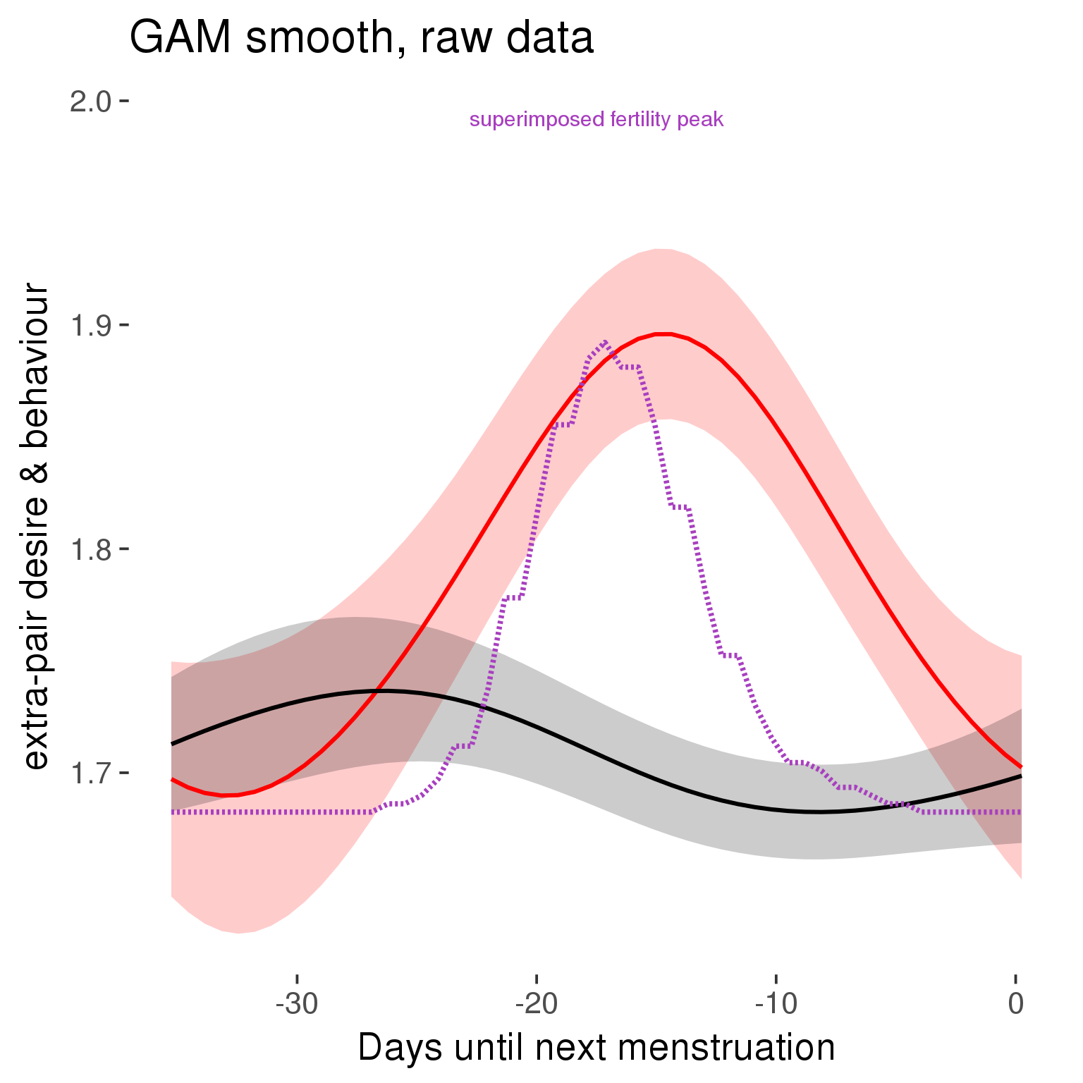
Means and standard errors over raw data
Nothing partialled out, just straight means with bootstrapped confidence intervals.
tryCatch({
  trend_plot = ggplot(tmp,aes_string(x = "RCD", y = outcome, colour = "included")) +
    geom_pointrange(size = 0.8, stat = 'summary', fun.data = "mean_cl_boot")
}, error = function(e){cat_message(e, "danger")})
tryCatch({
  trend_data = ggplot_build(trend_plot)$data[[1]]
}, error = function(e){cat_message(e, "danger")})

trend_data$RCD = round(trend_data$x)
trend_data = left_join(trend_data, tmp %>% select(real, RCD,fertile) %>% unique(), by = "RCD")
trend_data %>%
  filter(real == TRUE) %>%
  mutate(superimposed = ( ( (fertile - 0.01)/0.58) * (max(y)-min(y) ) ) + min(y) ) ->
  trend_data

plot3 = ggplot(trend_data) +
  geom_pointrange(aes(x = x, y = y, ymin = ymin,ymax = ymax, colour = factor(group)), size = 0.8, stat = "identity", alpha = 0.6, position = position_dodge(width = .5)) +
  scale_x_continuous("Days until next menstruation") +
  geom_line(aes(x= x, y = superimposed), color = "#a83fbf", size = 1, linetype = 'dashed') +
  annotate("text",x = mean(trend_data$x),  y = max(trend_data$superimposed,na.rm=T) + 0.1, label = 'superimposed fertility peak', color = "#a83fbf") +
  scale_y_continuous(outcome_label) +
  ggtitle("Means with standard errors, raw data") +
  scale_color_manual("Contraception status",values = c("2"="black","1"= "red"), labels = c("2"="hormonally\ncontracepting","1"="cycling"), guide = F) +
  scale_fill_manual("Contraception status",values = c("2"="black","1"= "red"), labels = c("2"="hormonally\ncontracepting","1"="cycling"), guide = F)
suppressWarnings(print(plot3))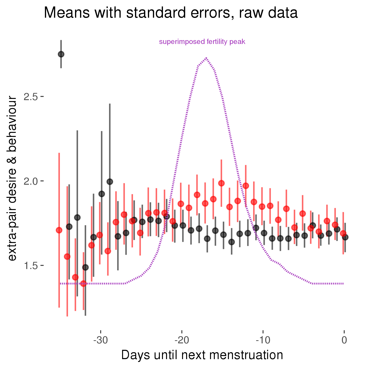
Forward-counted
model %>%
  plot_curve(diary %>% filter(minimum_cycle_length_diary <= 36, minimum_cycle_length_diary > 20) %>% mutate(RCD = FCD, fertile = prc_stirn_b_forward_counted), caption_x = "Days since last menstruation")
outcome = names(model@frame)[1]
outcome_label = recode(str_replace_all(str_replace_all(str_replace_all(outcome, "_", " "), " pair", "-pair"), " 1", ""),
"desirability 1" = "self-perceived desirability",
"NARQ admiration" = "narcissistic admiration",
"NARQ rivalry" = "narcissistic rivalry",
"extra-pair" = "extra-pair desire & behaviour",
"had sexual intercourse" = "sexual intercourse")
library(ggplot2)
# form a subset and run the model without the hormonal contraception and the fertility predictors
tmp = diary %>%
filter(!is.na(fertile), !is.na(included),
RCD > -1 * minimum_cycle_length_diary, RCD > -40)
new_form = update.formula(formula(model), new = . ~ . - fertile * included)
tmp$residuals = residuals(update(model, new_form, data = tmp , na.action = na.exclude))
tmp = tmp %>%
filter(!is.na(RCD), !is.na(residuals))
rcd_min = min(tmp$RCD)
tmp$real = FALSE
tmp_before = tmp
tmp_before$RCD = tmp_before$RCD + min(tmp$RCD) - 1
tmp_after = tmp
tmp_after$RCD = tmp_after$RCD - min(tmp$RCD) + 1
tmp$real = TRUE
tmp = bind_rows(tmp_before %>% filter(RCD > rcd_min - 11), tmp, tmp_after %>% filter(RCD < 11))GAM smooth on residuals
Here, we partialled out menstruation and individual random effects, then superimposed estimated probability of being in the fertile window scaled to the range of the estimated means. To address the periodicity of the cycle, we prepended and appended ten days of the timeseries to the end and the beginning of the timeseries. We then estimated the GAM and cut off the appended subsets before plotting.
tryCatch({
  trend_plot = ggplot(tmp,aes(x = RCD, y = residuals, colour = included)) +
    stat_smooth(geom = 'smooth',size = 0.8, fill = "#9ECAE1", method = 'gam', formula = y ~ s(x))
}, error = function(e){cat_message(e, "danger")})

tryCatch({
  trend_data = ggplot_build(trend_plot)$data[[1]]
}, error = function(e){cat_message(e, "danger")})

trend_data$RCD = round(trend_data$x)
trend_data = left_join(trend_data, tmp %>% select(real, RCD,fertile) %>% unique(), by = "RCD")
trend_data %>%
  filter(real == TRUE) %>%
  mutate(superimposed = ( ( (fertile - 0.01)/0.58) * (max(y)-min(y) ) ) + min(y) ) ->
  trend_data


ggplot(trend_data) +
  geom_ribbon(aes(x = x, ymin = ymin, ymax = ymax,  fill = factor(group)), alpha = 0.2) +
  geom_line(aes(x = x, y = y, colour = factor(group)), size = 0.8, stat = "identity") +
  scale_x_continuous(caption_x) +
  geom_line(aes(x = x, y = superimposed), color = "#a83fbf", size = 1, linetype = 'dashed') +
  annotate("text",x = mean(trend_data$x),  y = max(trend_data$superimposed,na.rm=T) + 0.1, label = 'superimposed fertility peak', color = "#a83fbf") +
  scale_y_continuous(outcome_label) +
  ggtitle("GAM smooth, residuals") +
  scale_color_manual("Contraception status",values = c("2"="black","1"= "red"), labels = c("2"="hormonally\ncontracepting","1"="cycling"), guide = F) +
  scale_fill_manual("Contraception status",values = c("2"="black","1"= "red"), labels = c("2"="hormonally\ncontracepting","1"="cycling"), guide = F)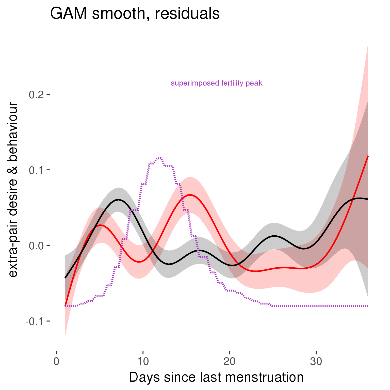
GAM smooth on raw data
As before, but without partialling anything out.
tryCatch({
  trend_plot = ggplot(tmp,aes_string(x = "RCD", y = outcome, colour = "included")) +
    stat_smooth(geom = 'smooth',size = 0.8, fill = "#9ECAE1", method = 'gam', formula = y ~ s(x))
}, error = function(e){cat_message(e, "danger")})

tryCatch({
  trend_data = ggplot_build(trend_plot)$data[[1]]
}, error = function(e){cat_message(e, "danger")})

trend_data$RCD = round(trend_data$x)
trend_data = left_join(trend_data, tmp %>% select(real, RCD,fertile) %>% unique(), by = "RCD")
trend_data %>%
  filter(real == TRUE) %>%
  mutate(superimposed = ( ( (fertile - 0.01)/0.58) * (max(y)-min(y) ) ) + min(y) ) ->
  trend_data

plot1b = ggplot(trend_data) +
  geom_ribbon(aes(x = x, ymin = ymin, ymax = ymax,  fill = factor(group)), alpha = 0.2) +
  geom_line(aes(x = x, y = y, colour = factor(group)), size = 0.8, stat = "identity") +
  scale_x_continuous(caption_x) +
  geom_line(aes(x = x, y = superimposed), color = "#a83fbf", size = 1, linetype = 'dashed') +
  annotate("text",x = mean(trend_data$x),  y = max(trend_data$superimposed,na.rm=T) + 0.1, label = 'superimposed fertility peak', color = "#a83fbf") +
  scale_y_continuous(outcome_label) +
  ggtitle("GAM smooth, raw data") +
  scale_color_manual("Contraception status",values = c("2"="black","1"= "red"), labels = c("2"="hormonally\ncontracepting","1"="cycling"), guide = F) +
  scale_fill_manual("Contraception status",values = c("2"="black","1"= "red"), labels = c("2"="hormonally\ncontracepting","1"="cycling"), guide = F)

suppressWarnings(print(plot1b))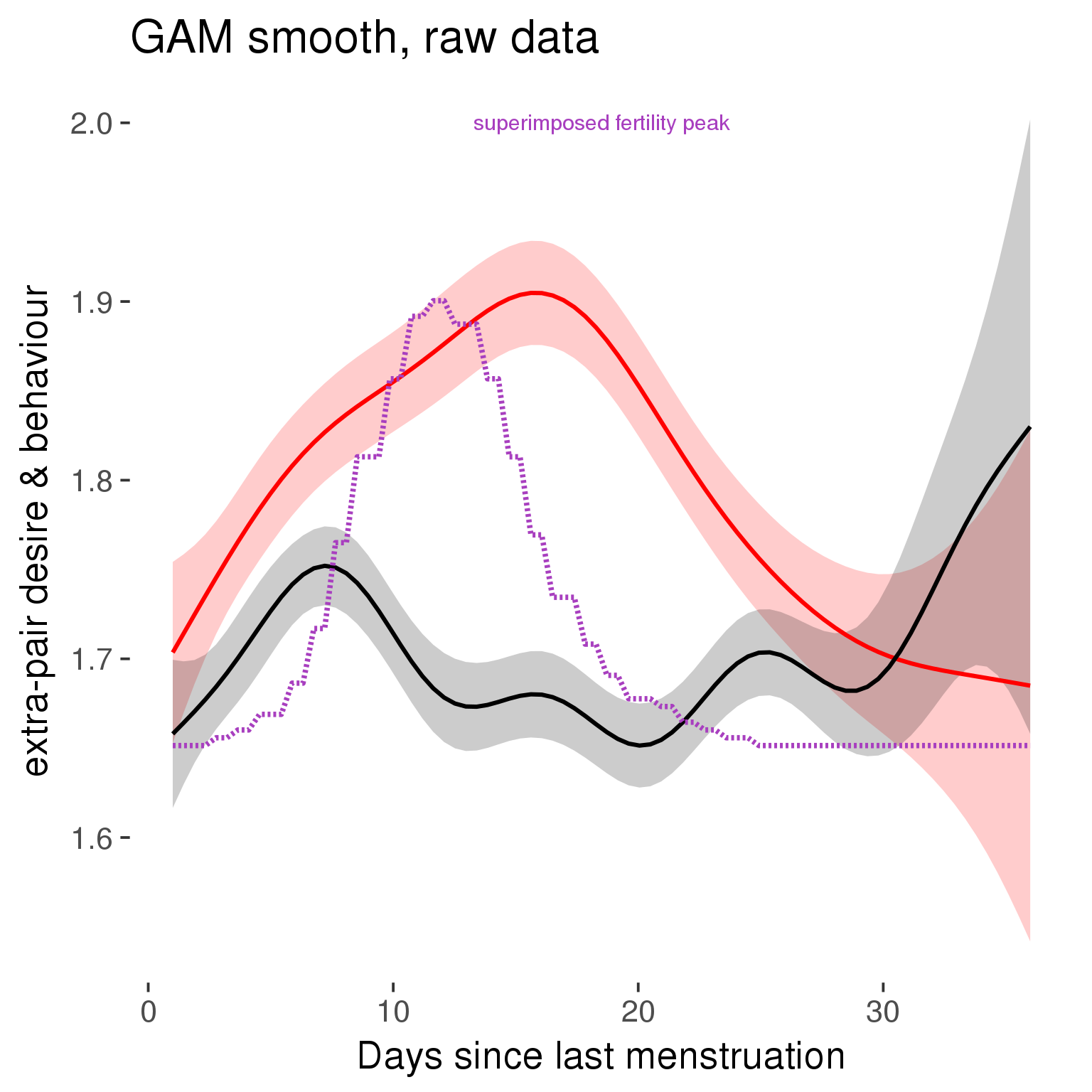
Means and standard errors over raw data
Nothing partialled out, just straight means with bootstrapped confidence intervals.
tryCatch({
  trend_plot = ggplot(tmp,aes_string(x = "RCD", y = outcome, colour = "included")) +
    geom_pointrange(size = 0.8, stat = 'summary', fun.data = "mean_cl_boot")
}, error = function(e){cat_message(e, "danger")})
tryCatch({
  trend_data = ggplot_build(trend_plot)$data[[1]]
}, error = function(e){cat_message(e, "danger")})

trend_data$RCD = round(trend_data$x)
trend_data = left_join(trend_data, tmp %>% select(real, RCD,fertile) %>% unique(), by = "RCD")
trend_data %>%
  filter(real == TRUE) %>%
  mutate(superimposed = ( ( (fertile - 0.01)/0.58) * (max(y)-min(y) ) ) + min(y) ) ->
  trend_data

plot3 = ggplot(trend_data) +
  geom_pointrange(aes(x = x, y = y, ymin = ymin,ymax = ymax, colour = factor(group)), size = 0.8, stat = "identity", alpha = 0.6, position = position_dodge(width = .5)) +
  scale_x_continuous("Days until next menstruation") +
  geom_line(aes(x= x, y = superimposed), color = "#a83fbf", size = 1, linetype = 'dashed') +
  annotate("text",x = mean(trend_data$x),  y = max(trend_data$superimposed,na.rm=T) + 0.1, label = 'superimposed fertility peak', color = "#a83fbf") +
  scale_y_continuous(outcome_label) +
  ggtitle("Means with standard errors, raw data") +
  scale_color_manual("Contraception status",values = c("2"="black","1"= "red"), labels = c("2"="hormonally\ncontracepting","1"="cycling"), guide = F) +
  scale_fill_manual("Contraception status",values = c("2"="black","1"= "red"), labels = c("2"="hormonally\ncontracepting","1"="cycling"), guide = F)
suppressWarnings(print(plot3))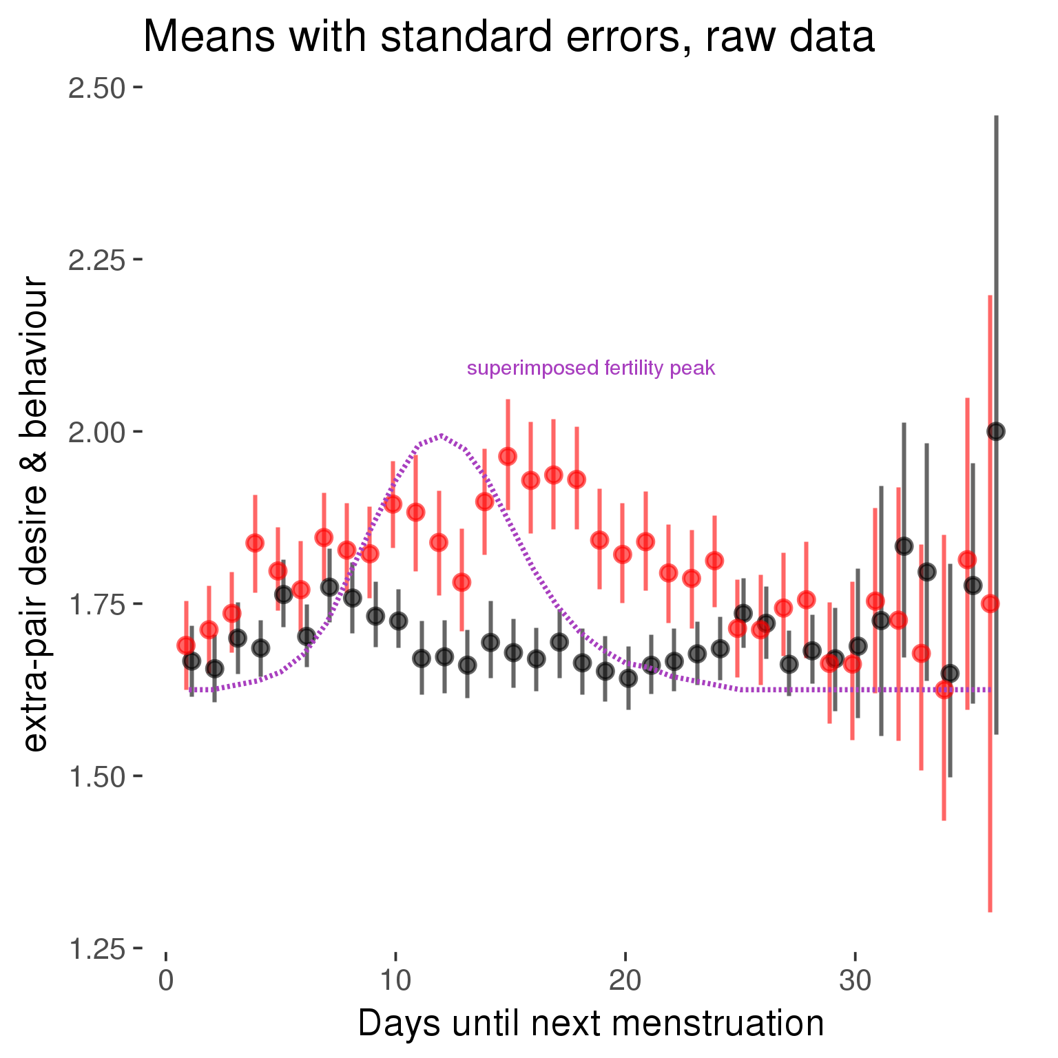
Cycle lengths from 27 to 30
Backward-counted
model %>%
  plot_curve(diary %>% filter(minimum_cycle_length_diary <= 30, minimum_cycle_length_diary >= 27) %>% mutate(fertile=prc_stirn_b))
outcome = names(model@frame)[1]
outcome_label = recode(str_replace_all(str_replace_all(str_replace_all(outcome, "_", " "), " pair", "-pair"), " 1", ""),
"desirability 1" = "self-perceived desirability",
"NARQ admiration" = "narcissistic admiration",
"NARQ rivalry" = "narcissistic rivalry",
"extra-pair" = "extra-pair desire & behaviour",
"had sexual intercourse" = "sexual intercourse")
library(ggplot2)
# form a subset and run the model without the hormonal contraception and the fertility predictors
tmp = diary %>%
filter(!is.na(fertile), !is.na(included),
RCD > -1 * minimum_cycle_length_diary, RCD > -40)
new_form = update.formula(formula(model), new = . ~ . - fertile * included)
tmp$residuals = residuals(update(model, new_form, data = tmp , na.action = na.exclude))
tmp = tmp %>%
filter(!is.na(RCD), !is.na(residuals))
rcd_min = min(tmp$RCD)
tmp$real = FALSE
tmp_before = tmp
tmp_before$RCD = tmp_before$RCD + min(tmp$RCD) - 1
tmp_after = tmp
tmp_after$RCD = tmp_after$RCD - min(tmp$RCD) + 1
tmp$real = TRUE
tmp = bind_rows(tmp_before %>% filter(RCD > rcd_min - 11), tmp, tmp_after %>% filter(RCD < 11))GAM smooth on residuals
Here, we partialled out menstruation and individual random effects, then superimposed estimated probability of being in the fertile window scaled to the range of the estimated means. To address the periodicity of the cycle, we prepended and appended ten days of the timeseries to the end and the beginning of the timeseries. We then estimated the GAM and cut off the appended subsets before plotting.
tryCatch({
  trend_plot = ggplot(tmp,aes(x = RCD, y = residuals, colour = included)) +
    stat_smooth(geom = 'smooth',size = 0.8, fill = "#9ECAE1", method = 'gam', formula = y ~ s(x))
}, error = function(e){cat_message(e, "danger")})

tryCatch({
  trend_data = ggplot_build(trend_plot)$data[[1]]
}, error = function(e){cat_message(e, "danger")})

trend_data$RCD = round(trend_data$x)
trend_data = left_join(trend_data, tmp %>% select(real, RCD,fertile) %>% unique(), by = "RCD")
trend_data %>%
  filter(real == TRUE) %>%
  mutate(superimposed = ( ( (fertile - 0.01)/0.58) * (max(y)-min(y) ) ) + min(y) ) ->
  trend_data


ggplot(trend_data) +
  geom_ribbon(aes(x = x, ymin = ymin, ymax = ymax,  fill = factor(group)), alpha = 0.2) +
  geom_line(aes(x = x, y = y, colour = factor(group)), size = 0.8, stat = "identity") +
  scale_x_continuous(caption_x) +
  geom_line(aes(x = x, y = superimposed), color = "#a83fbf", size = 1, linetype = 'dashed') +
  annotate("text",x = mean(trend_data$x),  y = max(trend_data$superimposed,na.rm=T) + 0.1, label = 'superimposed fertility peak', color = "#a83fbf") +
  scale_y_continuous(outcome_label) +
  ggtitle("GAM smooth, residuals") +
  scale_color_manual("Contraception status",values = c("2"="black","1"= "red"), labels = c("2"="hormonally\ncontracepting","1"="cycling"), guide = F) +
  scale_fill_manual("Contraception status",values = c("2"="black","1"= "red"), labels = c("2"="hormonally\ncontracepting","1"="cycling"), guide = F)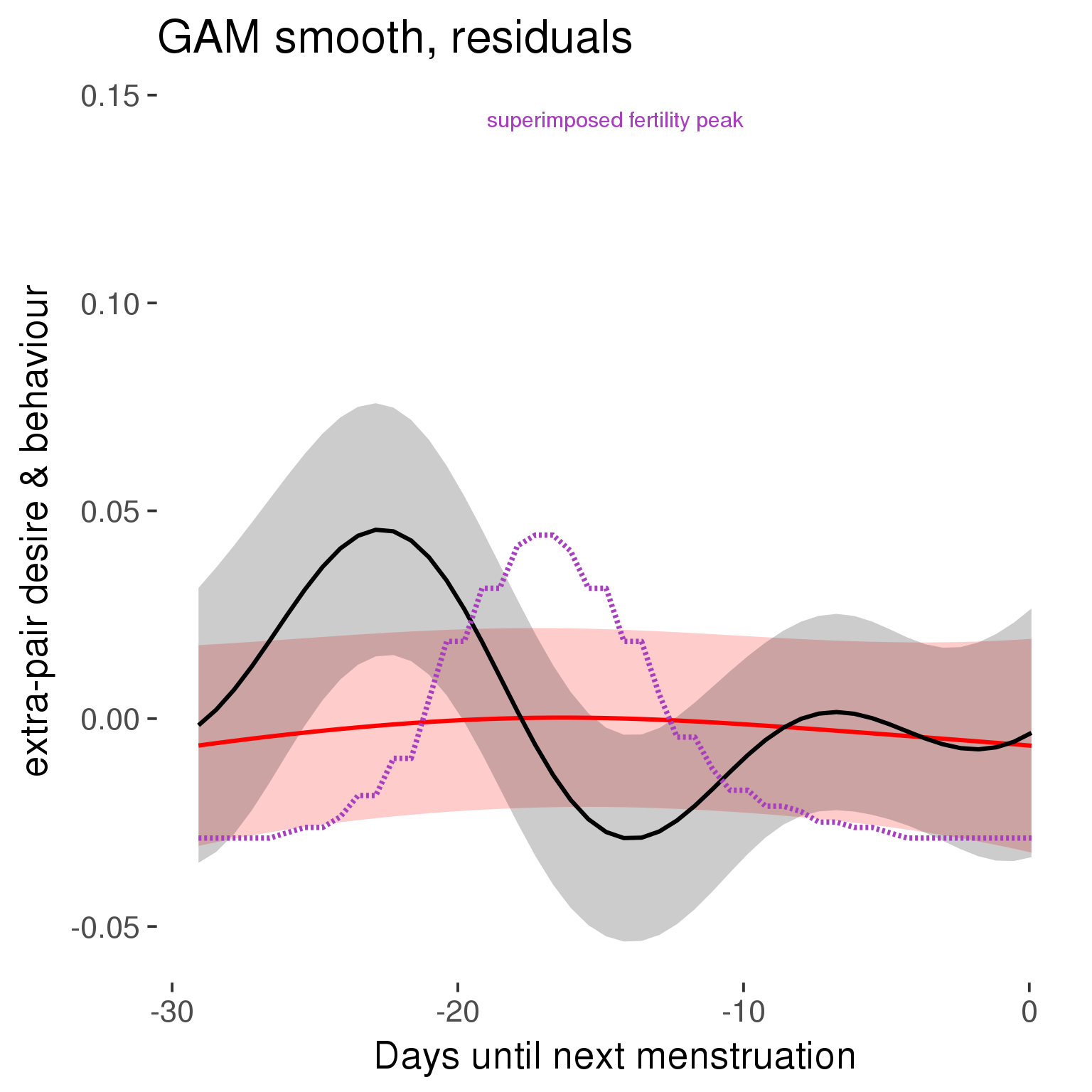
GAM smooth on raw data
As before, but without partialling anything out.
tryCatch({
  trend_plot = ggplot(tmp,aes_string(x = "RCD", y = outcome, colour = "included")) +
    stat_smooth(geom = 'smooth',size = 0.8, fill = "#9ECAE1", method = 'gam', formula = y ~ s(x))
}, error = function(e){cat_message(e, "danger")})

tryCatch({
  trend_data = ggplot_build(trend_plot)$data[[1]]
}, error = function(e){cat_message(e, "danger")})

trend_data$RCD = round(trend_data$x)
trend_data = left_join(trend_data, tmp %>% select(real, RCD,fertile) %>% unique(), by = "RCD")
trend_data %>%
  filter(real == TRUE) %>%
  mutate(superimposed = ( ( (fertile - 0.01)/0.58) * (max(y)-min(y) ) ) + min(y) ) ->
  trend_data

plot1b = ggplot(trend_data) +
  geom_ribbon(aes(x = x, ymin = ymin, ymax = ymax,  fill = factor(group)), alpha = 0.2) +
  geom_line(aes(x = x, y = y, colour = factor(group)), size = 0.8, stat = "identity") +
  scale_x_continuous(caption_x) +
  geom_line(aes(x = x, y = superimposed), color = "#a83fbf", size = 1, linetype = 'dashed') +
  annotate("text",x = mean(trend_data$x),  y = max(trend_data$superimposed,na.rm=T) + 0.1, label = 'superimposed fertility peak', color = "#a83fbf") +
  scale_y_continuous(outcome_label) +
  ggtitle("GAM smooth, raw data") +
  scale_color_manual("Contraception status",values = c("2"="black","1"= "red"), labels = c("2"="hormonally\ncontracepting","1"="cycling"), guide = F) +
  scale_fill_manual("Contraception status",values = c("2"="black","1"= "red"), labels = c("2"="hormonally\ncontracepting","1"="cycling"), guide = F)

suppressWarnings(print(plot1b))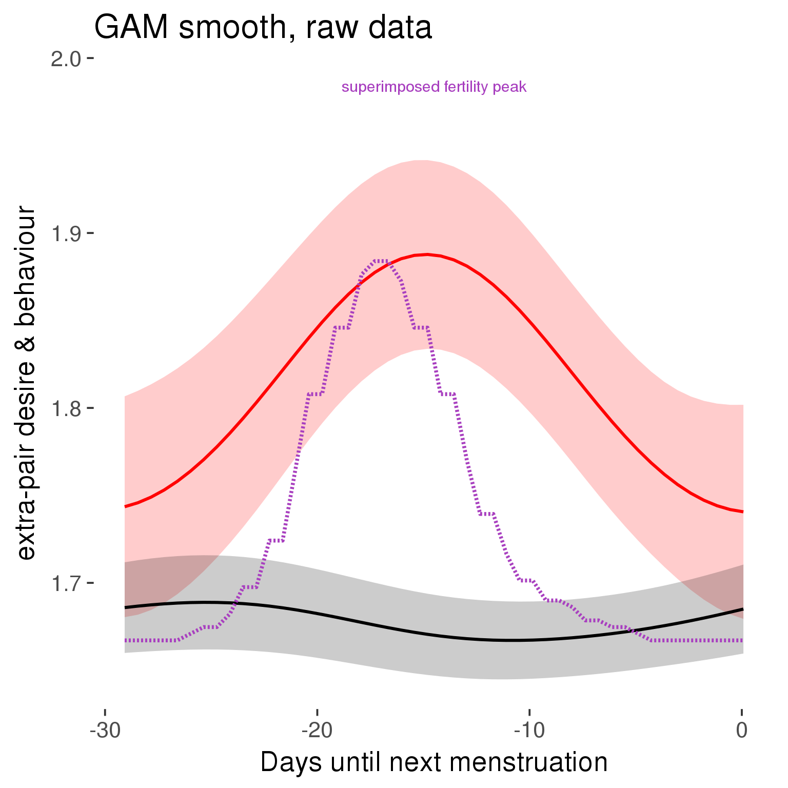
Means and standard errors over raw data
Nothing partialled out, just straight means with bootstrapped confidence intervals.
tryCatch({
  trend_plot = ggplot(tmp,aes_string(x = "RCD", y = outcome, colour = "included")) +
    geom_pointrange(size = 0.8, stat = 'summary', fun.data = "mean_cl_boot")
}, error = function(e){cat_message(e, "danger")})
tryCatch({
  trend_data = ggplot_build(trend_plot)$data[[1]]
}, error = function(e){cat_message(e, "danger")})

trend_data$RCD = round(trend_data$x)
trend_data = left_join(trend_data, tmp %>% select(real, RCD,fertile) %>% unique(), by = "RCD")
trend_data %>%
  filter(real == TRUE) %>%
  mutate(superimposed = ( ( (fertile - 0.01)/0.58) * (max(y)-min(y) ) ) + min(y) ) ->
  trend_data

plot3 = ggplot(trend_data) +
  geom_pointrange(aes(x = x, y = y, ymin = ymin,ymax = ymax, colour = factor(group)), size = 0.8, stat = "identity", alpha = 0.6, position = position_dodge(width = .5)) +
  scale_x_continuous("Days until next menstruation") +
  geom_line(aes(x= x, y = superimposed), color = "#a83fbf", size = 1, linetype = 'dashed') +
  annotate("text",x = mean(trend_data$x),  y = max(trend_data$superimposed,na.rm=T) + 0.1, label = 'superimposed fertility peak', color = "#a83fbf") +
  scale_y_continuous(outcome_label) +
  ggtitle("Means with standard errors, raw data") +
  scale_color_manual("Contraception status",values = c("2"="black","1"= "red"), labels = c("2"="hormonally\ncontracepting","1"="cycling"), guide = F) +
  scale_fill_manual("Contraception status",values = c("2"="black","1"= "red"), labels = c("2"="hormonally\ncontracepting","1"="cycling"), guide = F)
suppressWarnings(print(plot3))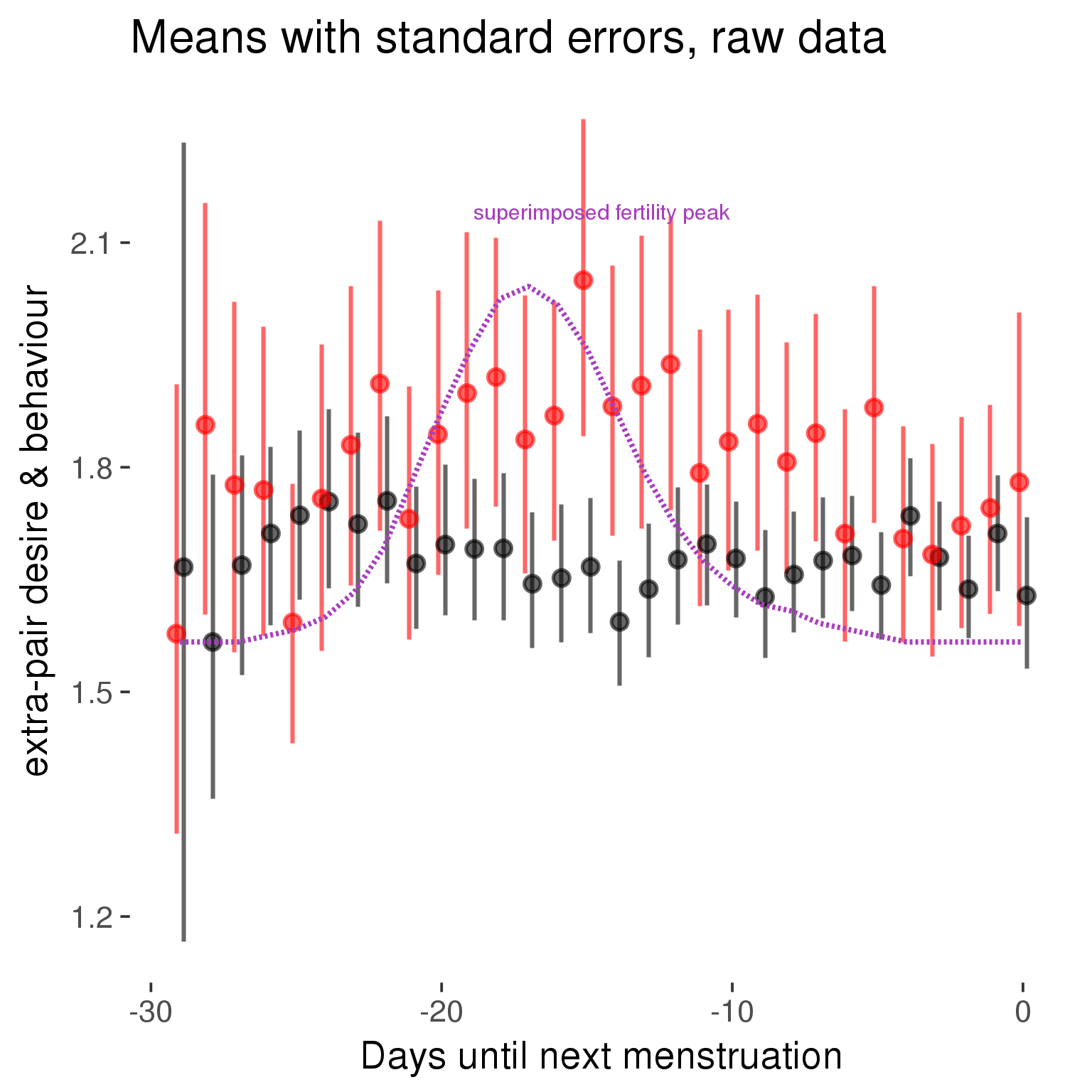
Forward-counted
model %>%
  plot_curve(diary %>% filter(minimum_cycle_length_diary <= 30, minimum_cycle_length_diary >= 27) %>% mutate(RCD = FCD, fertile = prc_stirn_b_forward_counted), caption_x = "Days since last menstruation")
outcome = names(model@frame)[1]
outcome_label = recode(str_replace_all(str_replace_all(str_replace_all(outcome, "_", " "), " pair", "-pair"), " 1", ""),
"desirability 1" = "self-perceived desirability",
"NARQ admiration" = "narcissistic admiration",
"NARQ rivalry" = "narcissistic rivalry",
"extra-pair" = "extra-pair desire & behaviour",
"had sexual intercourse" = "sexual intercourse")
library(ggplot2)
# form a subset and run the model without the hormonal contraception and the fertility predictors
tmp = diary %>%
filter(!is.na(fertile), !is.na(included),
RCD > -1 * minimum_cycle_length_diary, RCD > -40)
new_form = update.formula(formula(model), new = . ~ . - fertile * included)
tmp$residuals = residuals(update(model, new_form, data = tmp , na.action = na.exclude))
tmp = tmp %>%
filter(!is.na(RCD), !is.na(residuals))
rcd_min = min(tmp$RCD)
tmp$real = FALSE
tmp_before = tmp
tmp_before$RCD = tmp_before$RCD + min(tmp$RCD) - 1
tmp_after = tmp
tmp_after$RCD = tmp_after$RCD - min(tmp$RCD) + 1
tmp$real = TRUE
tmp = bind_rows(tmp_before %>% filter(RCD > rcd_min - 11), tmp, tmp_after %>% filter(RCD < 11))GAM smooth on residuals
Here, we partialled out menstruation and individual random effects, then superimposed estimated probability of being in the fertile window scaled to the range of the estimated means. To address the periodicity of the cycle, we prepended and appended ten days of the timeseries to the end and the beginning of the timeseries. We then estimated the GAM and cut off the appended subsets before plotting.
tryCatch({
  trend_plot = ggplot(tmp,aes(x = RCD, y = residuals, colour = included)) +
    stat_smooth(geom = 'smooth',size = 0.8, fill = "#9ECAE1", method = 'gam', formula = y ~ s(x))
}, error = function(e){cat_message(e, "danger")})

tryCatch({
  trend_data = ggplot_build(trend_plot)$data[[1]]
}, error = function(e){cat_message(e, "danger")})

trend_data$RCD = round(trend_data$x)
trend_data = left_join(trend_data, tmp %>% select(real, RCD,fertile) %>% unique(), by = "RCD")
trend_data %>%
  filter(real == TRUE) %>%
  mutate(superimposed = ( ( (fertile - 0.01)/0.58) * (max(y)-min(y) ) ) + min(y) ) ->
  trend_data


ggplot(trend_data) +
  geom_ribbon(aes(x = x, ymin = ymin, ymax = ymax,  fill = factor(group)), alpha = 0.2) +
  geom_line(aes(x = x, y = y, colour = factor(group)), size = 0.8, stat = "identity") +
  scale_x_continuous(caption_x) +
  geom_line(aes(x = x, y = superimposed), color = "#a83fbf", size = 1, linetype = 'dashed') +
  annotate("text",x = mean(trend_data$x),  y = max(trend_data$superimposed,na.rm=T) + 0.1, label = 'superimposed fertility peak', color = "#a83fbf") +
  scale_y_continuous(outcome_label) +
  ggtitle("GAM smooth, residuals") +
  scale_color_manual("Contraception status",values = c("2"="black","1"= "red"), labels = c("2"="hormonally\ncontracepting","1"="cycling"), guide = F) +
  scale_fill_manual("Contraception status",values = c("2"="black","1"= "red"), labels = c("2"="hormonally\ncontracepting","1"="cycling"), guide = F)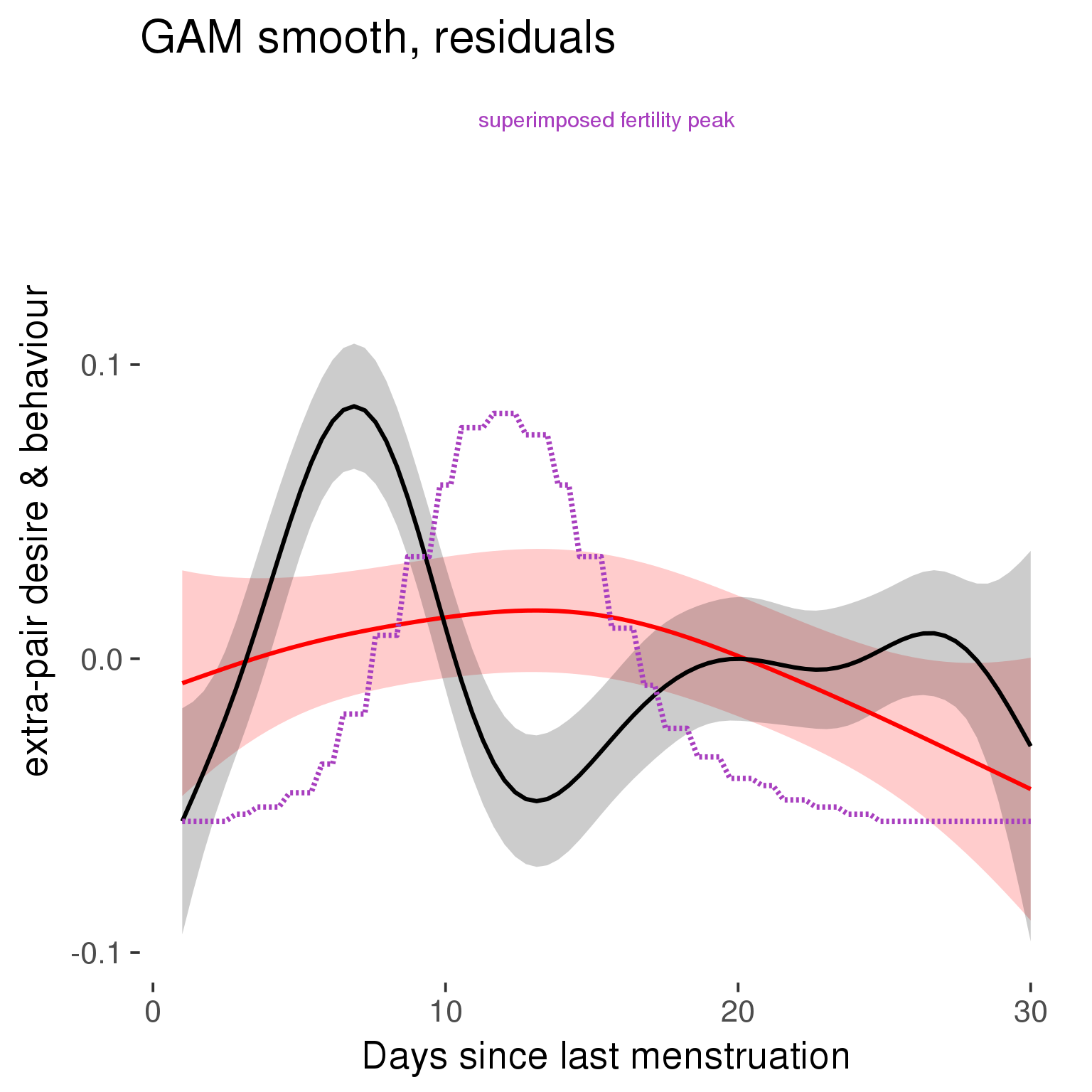
GAM smooth on raw data
As before, but without partialling anything out.
tryCatch({
  trend_plot = ggplot(tmp,aes_string(x = "RCD", y = outcome, colour = "included")) +
    stat_smooth(geom = 'smooth',size = 0.8, fill = "#9ECAE1", method = 'gam', formula = y ~ s(x))
}, error = function(e){cat_message(e, "danger")})

tryCatch({
  trend_data = ggplot_build(trend_plot)$data[[1]]
}, error = function(e){cat_message(e, "danger")})

trend_data$RCD = round(trend_data$x)
trend_data = left_join(trend_data, tmp %>% select(real, RCD,fertile) %>% unique(), by = "RCD")
trend_data %>%
  filter(real == TRUE) %>%
  mutate(superimposed = ( ( (fertile - 0.01)/0.58) * (max(y)-min(y) ) ) + min(y) ) ->
  trend_data

plot1b = ggplot(trend_data) +
  geom_ribbon(aes(x = x, ymin = ymin, ymax = ymax,  fill = factor(group)), alpha = 0.2) +
  geom_line(aes(x = x, y = y, colour = factor(group)), size = 0.8, stat = "identity") +
  scale_x_continuous(caption_x) +
  geom_line(aes(x = x, y = superimposed), color = "#a83fbf", size = 1, linetype = 'dashed') +
  annotate("text",x = mean(trend_data$x),  y = max(trend_data$superimposed,na.rm=T) + 0.1, label = 'superimposed fertility peak', color = "#a83fbf") +
  scale_y_continuous(outcome_label) +
  ggtitle("GAM smooth, raw data") +
  scale_color_manual("Contraception status",values = c("2"="black","1"= "red"), labels = c("2"="hormonally\ncontracepting","1"="cycling"), guide = F) +
  scale_fill_manual("Contraception status",values = c("2"="black","1"= "red"), labels = c("2"="hormonally\ncontracepting","1"="cycling"), guide = F)

suppressWarnings(print(plot1b))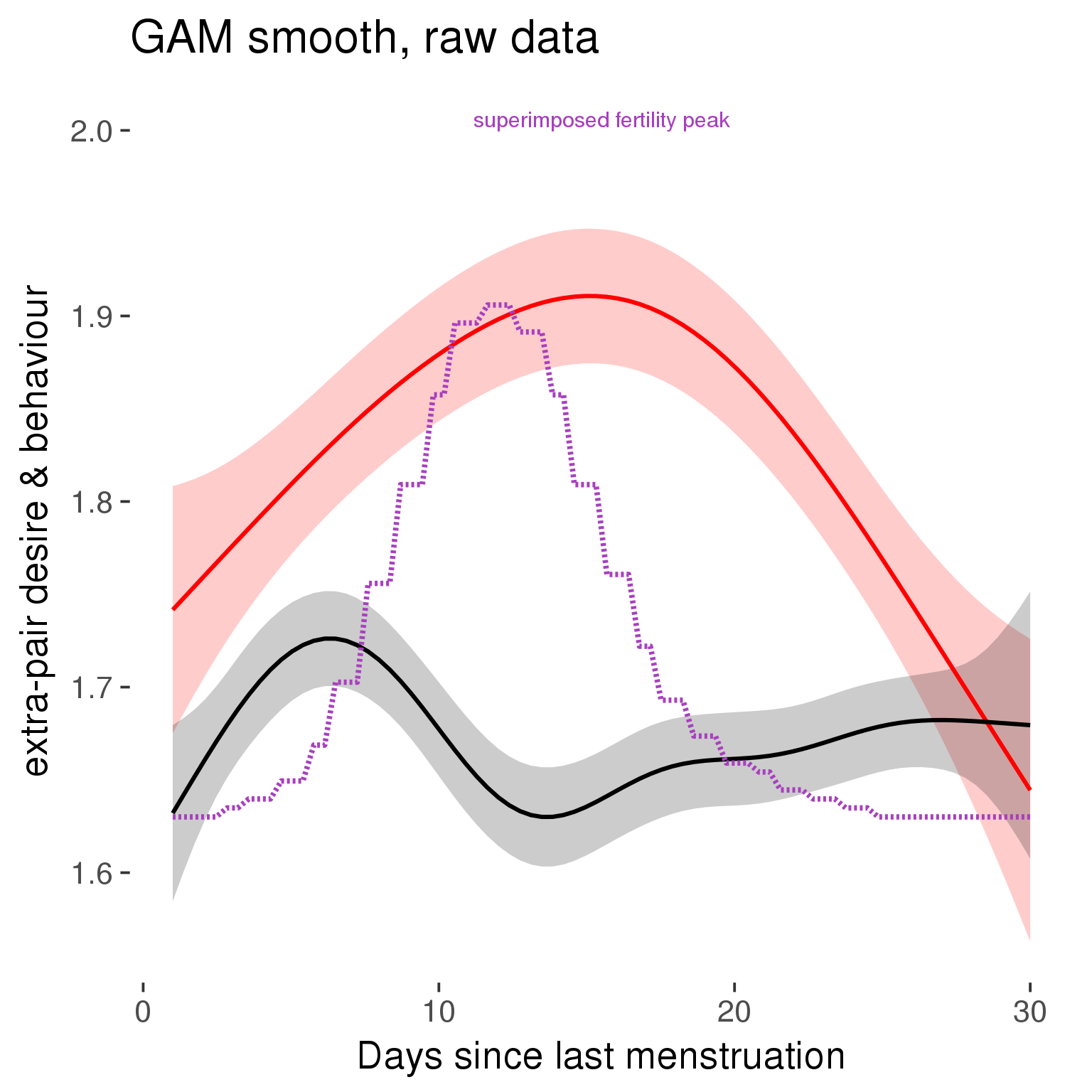
Means and standard errors over raw data
Nothing partialled out, just straight means with bootstrapped confidence intervals.
tryCatch({
  trend_plot = ggplot(tmp,aes_string(x = "RCD", y = outcome, colour = "included")) +
    geom_pointrange(size = 0.8, stat = 'summary', fun.data = "mean_cl_boot")
}, error = function(e){cat_message(e, "danger")})
tryCatch({
  trend_data = ggplot_build(trend_plot)$data[[1]]
}, error = function(e){cat_message(e, "danger")})

trend_data$RCD = round(trend_data$x)
trend_data = left_join(trend_data, tmp %>% select(real, RCD,fertile) %>% unique(), by = "RCD")
trend_data %>%
  filter(real == TRUE) %>%
  mutate(superimposed = ( ( (fertile - 0.01)/0.58) * (max(y)-min(y) ) ) + min(y) ) ->
  trend_data

plot3 = ggplot(trend_data) +
  geom_pointrange(aes(x = x, y = y, ymin = ymin,ymax = ymax, colour = factor(group)), size = 0.8, stat = "identity", alpha = 0.6, position = position_dodge(width = .5)) +
  scale_x_continuous("Days until next menstruation") +
  geom_line(aes(x= x, y = superimposed), color = "#a83fbf", size = 1, linetype = 'dashed') +
  annotate("text",x = mean(trend_data$x),  y = max(trend_data$superimposed,na.rm=T) + 0.1, label = 'superimposed fertility peak', color = "#a83fbf") +
  scale_y_continuous(outcome_label) +
  ggtitle("Means with standard errors, raw data") +
  scale_color_manual("Contraception status",values = c("2"="black","1"= "red"), labels = c("2"="hormonally\ncontracepting","1"="cycling"), guide = F) +
  scale_fill_manual("Contraception status",values = c("2"="black","1"= "red"), labels = c("2"="hormonally\ncontracepting","1"="cycling"), guide = F)
suppressWarnings(print(plot3))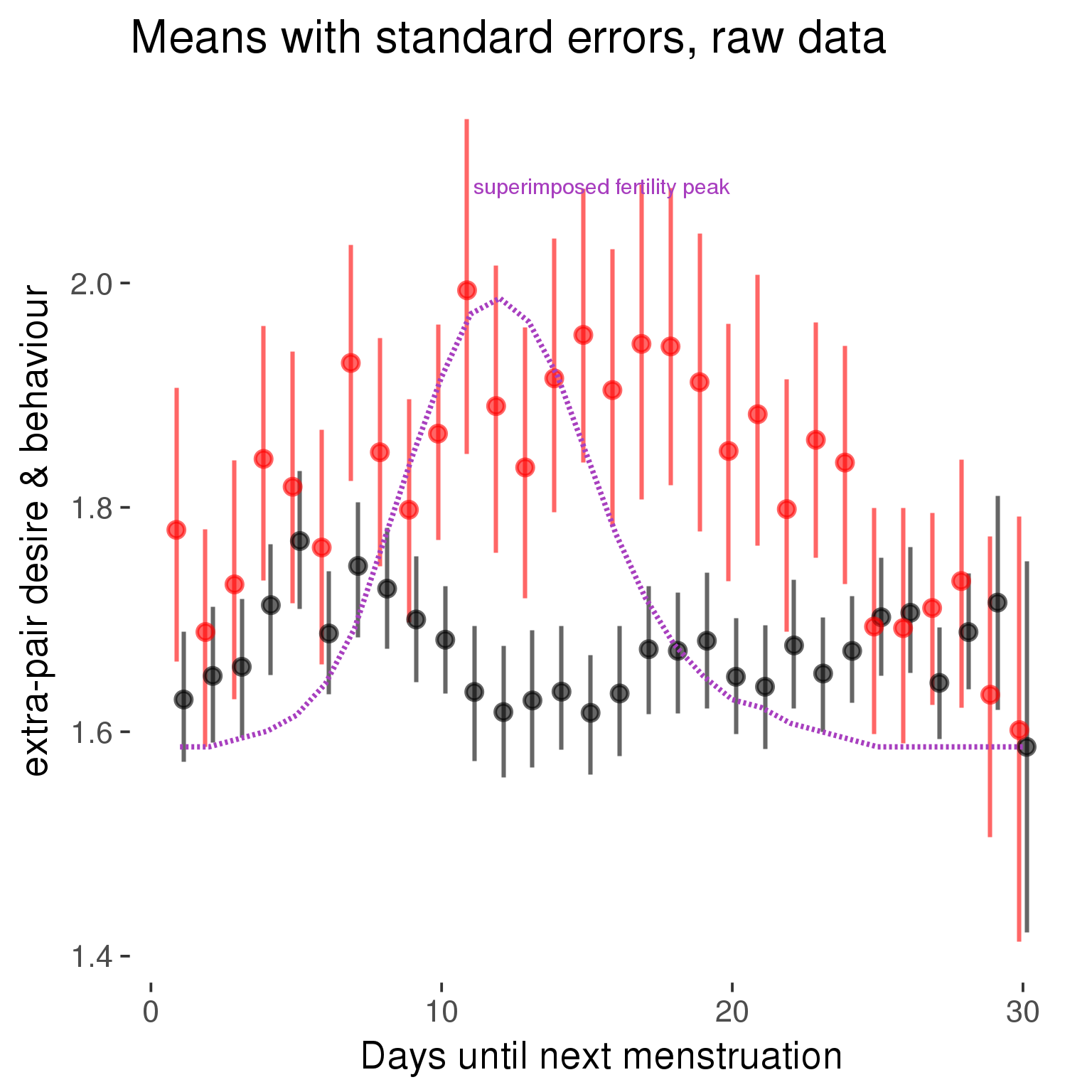
Robustness checks
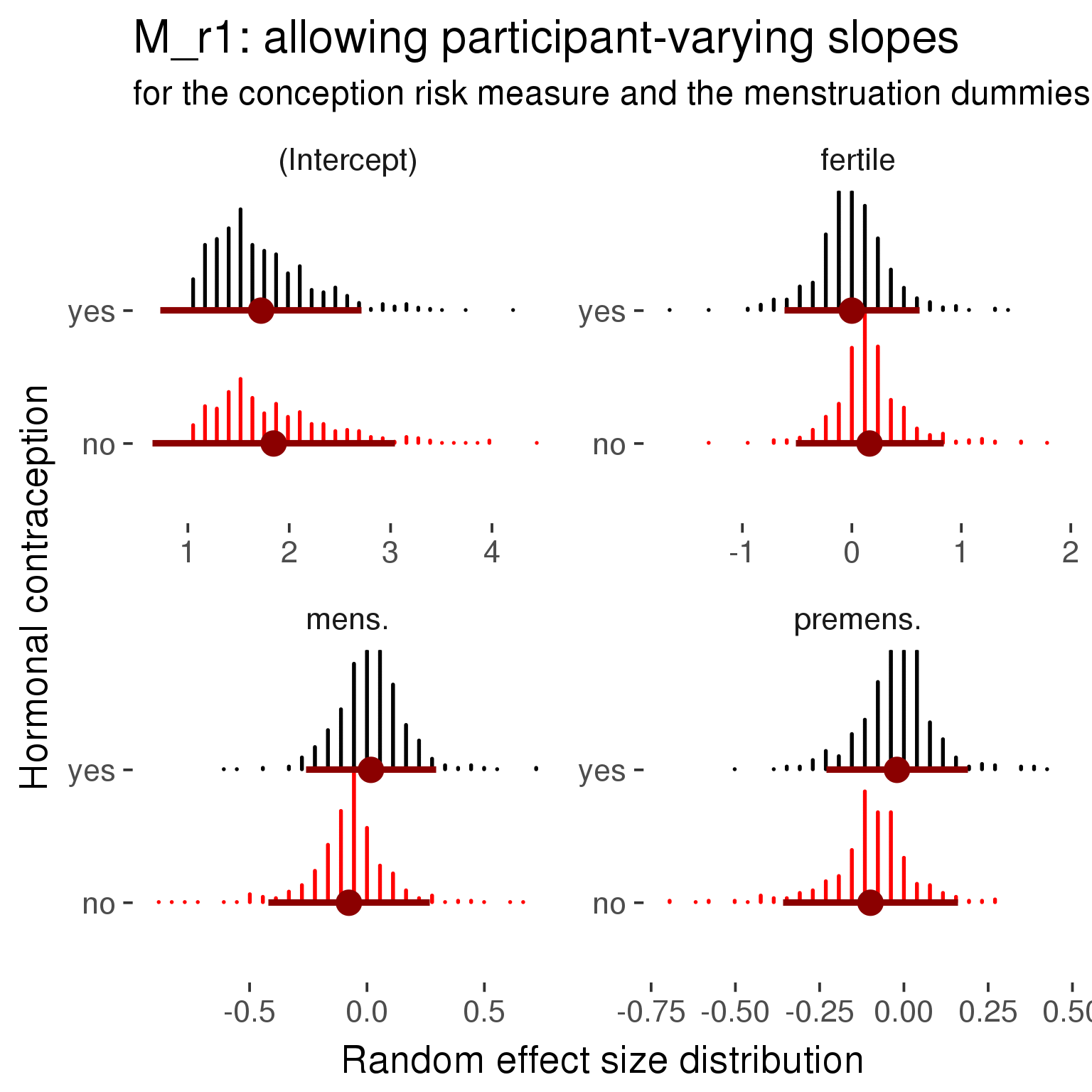
M_r1: Random slopes for conception risk and menstruation
tryCatch({
# refit model with random effects for fertile and menstruation dummies
with_ind_diff = update(model, formula = . ~ . - (1| person) + (1 + fertile + menstruation | person))

# pull the random effects, format as tibble
rand = coef(with_ind_diff)$person %>%
  tibble::rownames_to_column("person") %>%
  mutate(person = as.numeric(person))

# pull the fixed effects
fixd = data.frame(fixef(with_ind_diff)) %>%
  tibble::rownames_to_column("effect")
names(fixd) = c("effect", "pop_effect_size")

# pull apart the coefficients so that we can account for the fact that the random effect variation implicitly includes HC explaining the mean population-level effect of fertile/menstruation dummies among HC users
fixd = fixd %>%
  separate(effect, c("included", "effect"), sep = ":", fill = "left") %>%
  mutate(included = if_else(is.na(included), "cycling", str_replace(included, "included", "")))
fixd[2,c("included", "effect")] = c("horm_contra", "(Intercept)")


rand = rand %>%
  # merge diary data on the random effects, so that we know who is a HC users and who isn't
  inner_join(diary %>% select(person, included) %>% unique(), by = 'person') %>%
  # gather into long format, to have the dataset by predictor
  gather(effect, value, -person, -included) %>%
  inner_join(fixd, by = c('effect', 'included')) %>%
  # pull the fixed effects
  mutate(
    # only for those who are HC users, add the moderated population effect size for this effect (the random effects have the reference category mean)
    value = if_else(included == "horm_contra", value + pop_effect_size, value),
    effect = recode(effect, "includedhorm_contra" = "HC user",
                   "includedhorm_contra:fertile" = "HC user x fertile",
                   "includedhorm_contra:menstruationpre" = "HC user x premens.",
                   "includedhorm_contra:menstruationyes" = "HC user x mens.",
                   "menstruationyes" = "mens.",
                   "menstruationpre" = "premens.")) %>%
  group_by(included, effect) %>%
  # filter out predictors that aren't modelled as varying/random
  filter(sd(value) > 0)

# plot dot plot of random effects
print(
ggplot(rand, aes(x = included, y = value, color = included, fill = included)) +
  facet_wrap( ~ effect, scales = "free") +
  # geom_violin(alpha = 0.4, size = 0) +
  geom_dotplot(binaxis='y', dotsize = 0.1, method = "histodot") +
# geom_jitter(alpha = 0.05) +
  coord_flip() +
  geom_pointrange(stat = 'summary', fun.data = 'mean_sdl', color = 'darkred', size = 1.2) +
  scale_color_manual("Contraception status", values = c("horm_contra"="black","cycling"= "red"), labels = c("horm_contra"="hormonally\ncontracepting","cycling"="cycling"), guide = F) +
  scale_fill_manual("Contraception status", values = c("horm_contra"="black","cycling"= "red"), labels = c("horm_contra"="hormonally\ncontracepting","1"="cycling"), guide = F) +
  ggtitle("M_r1: allowing participant-varying slopes", subtitle = "for the conception risk measure and the menstruation dummies") +
  scale_x_discrete("Hormonal contraception", breaks = c("horm_contra", "cycling"), labels = c("yes", "no")) +
  scale_y_continuous("Random effect size distribution"))

print_summary(with_ind_diff)
cat(pander(anova(model, with_ind_diff)))
}, error = function(e){
  with_ind_diff = model
  cat_message(e, "danger")
})
Linear mixed model fit by REML ['lmerMod']
Formula: extra_pair ~ included + menstruation + fertile + fertile_mean +
    (1 + fertile + menstruation | person) + included:menstruation +      included:fertile
   Data: diary

REML criterion at convergence: 48206

Scaled residuals:
   Min     1Q Median     3Q    Max
-4.748 -0.550 -0.137  0.390  7.911

Random effects:
 Groups   Name            Variance Std.Dev. Corr
 person   (Intercept)     0.3328   0.577
          fertile         0.2900   0.538    -0.18
          menstruationpre 0.0442   0.210    -0.29  0.43
          menstruationyes 0.0672   0.259    -0.26  0.57  0.77
 Residual                 0.3029   0.550
Number of obs: 26680, groups:  person, 1054

Fixed effects:
                                    Estimate Std. Error t value
(Intercept)                           1.8464     0.0479    38.6
includedhorm_contra                  -0.1239     0.0399    -3.1
menstruationpre                      -0.0992     0.0208    -4.8
menstruationyes                      -0.0770     0.0216    -3.6
fertile                               0.1619     0.0459     3.5
fertile_mean                         -0.0983     0.2175    -0.5
includedhorm_contra:menstruationpre   0.0786     0.0267     2.9
includedhorm_contra:menstruationyes   0.0938     0.0281     3.3
includedhorm_contra:fertile          -0.1620     0.0583    -2.8

Correlation of Fixed Effects:
                        (Intr) incld_ mnstrtnp mnstrtny fertil frtl_m inclddhrm_cntr:mnstrtnp
inclddhrm_c             -0.481
menstrutnpr             -0.214  0.258
menstrutnys             -0.204  0.251  0.530
fertile                 -0.164  0.257  0.443    0.458
fertile_men             -0.764 -0.025 -0.001   -0.007   -0.064
inclddhrm_cntr:mnstrtnp  0.173 -0.327 -0.779   -0.412   -0.344 -0.007
inclddhrm_cntr:mnstrtny  0.164 -0.314 -0.407   -0.769   -0.352 -0.004  0.520
inclddhrm_cntr:f         0.159 -0.325 -0.348   -0.360   -0.784  0.011  0.443
                        inclddhrm_cntr:mnstrtny
inclddhrm_c
menstrutnpr
menstrutnys
fertile
fertile_men
inclddhrm_cntr:mnstrtnp
inclddhrm_cntr:mnstrtny
inclddhrm_cntr:f         0.455
refitting model(s) with ML (instead of REML)
| Df | AIC | BIC | logLik | deviance | Chisq | Chi Df | Pr(>Chisq) | |
|---|---|---|---|---|---|---|---|---|
| object | 11 | 48522 | 48612 | -24250 | 48500 | NA | NA | NA |
| ..1 | 20 | 48199 | 48362 | -24079 | 48159 | 341.2 | 9 | 4.584e-68 |
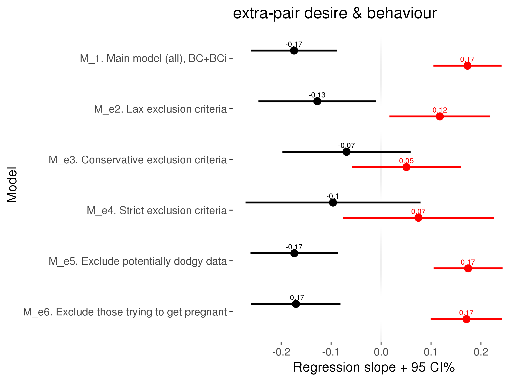
robustness_check_ovu_shift(model, diary)M_e: Exclusion criteria
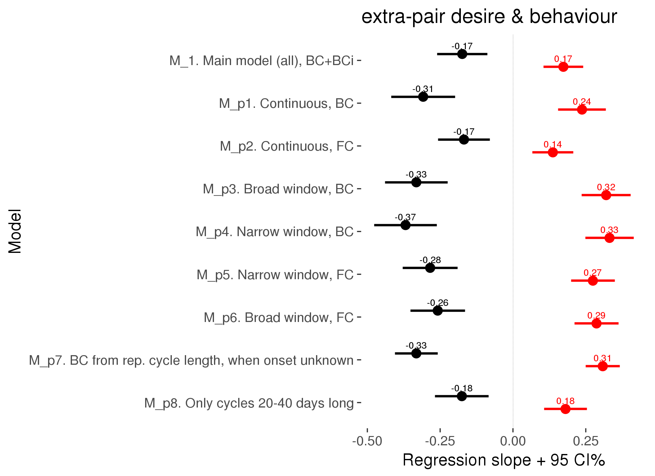
M_p: Predictors
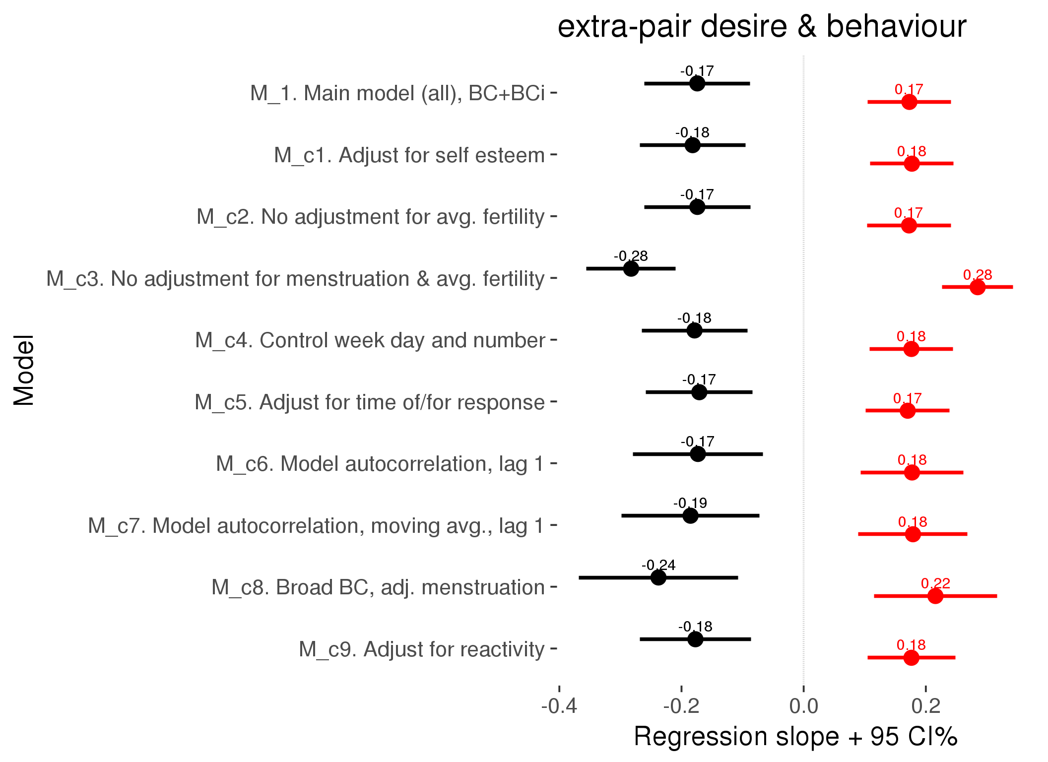
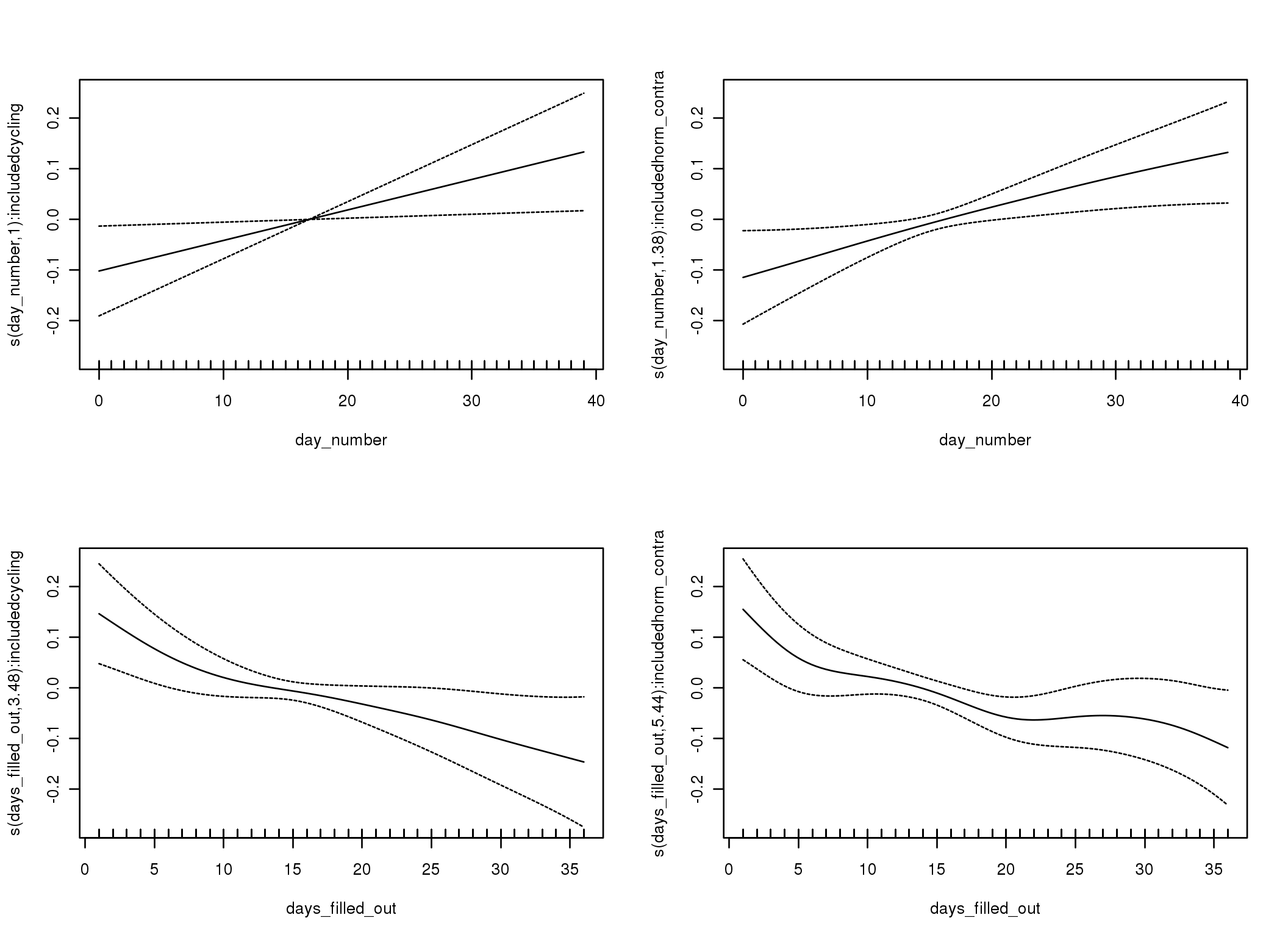
M_c: Covariates, controls, autocorrelation
Linear mixed model fit by REML ['lmerMod']

REML criterion at convergence: 43998

Scaled residuals:
   Min     1Q Median     3Q    Max
-4.439 -0.556 -0.143  0.402  8.138

Random effects:
 Groups   Name                                   Variance Std.Dev.
 person   (Intercept)                            0.3144   0.561
 Xr.2     s(days_filled_out):includedhorm_contra 0.0722   0.269
 Xr.1     s(days_filled_out):includedcycling     0.0159   0.126
 Xr.0     s(day_number):includedhorm_contra      0.0013   0.036
 Xr       s(day_number):includedcycling          0.0000   0.000
 Residual                                        0.3124   0.559
Number of obs: 24377, groups:  person, 1054; Xr.2, 8; Xr.1, 8; Xr.0, 8; Xr, 8

Fixed effects:
                                           Estimate Std. Error t value
X(Intercept)                                 1.8261     0.0473    38.6
Xincludedhorm_contra                        -0.1081     0.0391    -2.8
Xmenstruationpre                            -0.0925     0.0179    -5.2
Xmenstruationyes                            -0.0678     0.0172    -4.0
Xfertile                                     0.1764     0.0368     4.8
Xfertile_mean                               -0.0893     0.2147    -0.4
Xincludedhorm_contra:menstruationpre         0.0748     0.0229     3.3
Xincludedhorm_contra:menstruationyes         0.0865     0.0225     3.9
Xincludedhorm_contra:fertile                -0.1772     0.0466    -3.8
Xs(day_number):includedcyclingFx1            0.0683     0.0297     2.3
Xs(day_number):includedhorm_contraFx1        0.0694     0.0306     2.3
Xs(days_filled_out):includedcyclingFx1      -0.1257     0.0474    -2.7
Xs(days_filled_out):includedhorm_contraFx1  -0.2013     0.0612    -3.3
Family: gaussian
Link function: identity

Formula:
extra_pair ~ included + menstruation + fertile + fertile_mean +
    s(day_number, by = included) + s(days_filled_out, by = included) +
    included:menstruation + included:fertile

Parametric coefficients:
                                    Estimate Std. Error t value   Pr(>|t|)
(Intercept)                           1.8261     0.0473   38.59    < 2e-16 ***
includedhorm_contra                  -0.1081     0.0391   -2.76    0.00573 **
menstruationpre                      -0.0925     0.0179   -5.18 0.00000022 ***
menstruationyes                      -0.0678     0.0172   -3.95 0.00007773 ***
fertile                               0.1764     0.0368    4.80 0.00000163 ***
fertile_mean                         -0.0893     0.2147   -0.42    0.67753
includedhorm_contra:menstruationpre   0.0748     0.0229    3.26    0.00110 **
includedhorm_contra:menstruationyes   0.0865     0.0225    3.85    0.00012 ***
includedhorm_contra:fertile          -0.1772     0.0466   -3.80    0.00014 ***
---
Signif. codes:  0 '***' 0.001 '**' 0.01 '*' 0.05 '.' 0.1 ' ' 1

Approximate significance of smooth terms:
                                        edf Ref.df    F p-value
s(day_number):includedcycling          1.00   1.00 5.28  0.0216 *
s(day_number):includedhorm_contra      1.38   1.38 5.84  0.0162 *
s(days_filled_out):includedcycling     3.48   3.48 2.97  0.0150 *
s(days_filled_out):includedhorm_contra 5.44   5.44 3.18  0.0036 **
---
Signif. codes:  0 '***' 0.001 '**' 0.01 '*' 0.05 '.' 0.1 ' ' 1

R-sq.(adj) =  0.00548
lmer.REML =  43998  Scale est. = 0.31242   n = 24377
Linear mixed-effects model fit by REML
 Data: diary
    AIC   BIC logLik
  46934 47033 -23455

Random effects:
 Formula: ~1 | person
        (Intercept) Residual
StdDev:      0.5537    0.576

Correlation Structure: ARMA(1,0)
 Formula: ~day_number | person
 Parameter estimate(s):
  Phi1
0.3069
Fixed effects: extra_pair ~ included * (menstruation + fertile) + fertile_mean
                                      Value Std.Error    DF t-value p-value
(Intercept)                          1.8428   0.04799 25620   38.40  0.0000
includedhorm_contra                 -0.1181   0.03956  1051   -2.99  0.0029
menstruationpre                     -0.0883   0.02017 25620   -4.38  0.0000
menstruationyes                     -0.0684   0.01883 25620   -3.63  0.0003
fertile                              0.1774   0.04304 25620    4.12  0.0000
fertile_mean                        -0.0722   0.21899  1051   -0.33  0.7417
includedhorm_contra:menstruationpre  0.0726   0.02591 25620    2.80  0.0051
includedhorm_contra:menstruationyes  0.0843   0.02454 25620    3.43  0.0006
includedhorm_contra:fertile         -0.1731   0.05447 25620   -3.18  0.0015
 Correlation:
                                    (Intr) incld_ mnstrtnp mnstrtny fertil frtl_m inclddhrm_cntr:mnstrtnp
includedhorm_contra                 -0.477
menstruationpre                     -0.159  0.200
menstruationyes                     -0.156  0.195  0.404
fertile                             -0.153  0.255  0.425    0.360
fertile_mean                        -0.769 -0.024 -0.008   -0.006   -0.073
includedhorm_contra:menstruationpre  0.130 -0.249 -0.778   -0.314   -0.330 -0.003
includedhorm_contra:menstruationyes  0.125 -0.238 -0.310   -0.767   -0.275 -0.002  0.389
includedhorm_contra:fertile          0.155 -0.322 -0.335   -0.284   -0.787  0.013  0.424
                                    inclddhrm_cntr:mnstrtny
includedhorm_contra
menstruationpre
menstruationyes
fertile
fertile_mean
includedhorm_contra:menstruationpre
includedhorm_contra:menstruationyes
includedhorm_contra:fertile          0.353

Standardized Within-Group Residuals:
    Min      Q1     Med      Q3     Max
-4.2860 -0.5602 -0.1651  0.3831  7.8217

Number of Observations: 26680
Number of Groups: 1054
Linear mixed-effects model fit by REML
 Data: diary
    AIC   BIC logLik
  46632 46739 -23303

Random effects:
 Formula: ~1 | person
        (Intercept) Residual
StdDev:      0.5397    0.587

Correlation Structure: ARMA(1,1)
 Formula: ~day_number | person
 Parameter estimate(s):
   Phi1  Theta1
 0.7473 -0.4957
Fixed effects: extra_pair ~ included * (menstruation + fertile) + fertile_mean
                                      Value Std.Error    DF t-value p-value
(Intercept)                          1.8380   0.04804 25620   38.26  0.0000
includedhorm_contra                 -0.1123   0.03956  1051   -2.84  0.0046
menstruationpre                     -0.0769   0.02024 25620   -3.80  0.0001
menstruationyes                     -0.0622   0.01928 25620   -3.23  0.0013
fertile                              0.1790   0.04556 25620    3.93  0.0001
fertile_mean                        -0.0607   0.21991  1051   -0.28  0.7827
includedhorm_contra:menstruationpre  0.0606   0.02603 25620    2.33  0.0200
includedhorm_contra:menstruationyes  0.0702   0.02501 25620    2.81  0.0050
includedhorm_contra:fertile         -0.1853   0.05757 25620   -3.22  0.0013
 Correlation:
                                    (Intr) incld_ mnstrtnp mnstrtny fertil frtl_m inclddhrm_cntr:mnstrtnp
includedhorm_contra                 -0.475
menstruationpre                     -0.156  0.193
menstruationyes                     -0.160  0.199  0.435
fertile                             -0.151  0.258  0.353    0.337
fertile_mean                        -0.769 -0.027 -0.003   -0.005   -0.079
includedhorm_contra:menstruationpre  0.126 -0.240 -0.778   -0.338   -0.274 -0.003
includedhorm_contra:menstruationyes  0.128 -0.243 -0.335   -0.771   -0.260 -0.002  0.423
includedhorm_contra:fertile          0.156 -0.326 -0.279   -0.267   -0.788  0.014  0.352
                                    inclddhrm_cntr:mnstrtny
includedhorm_contra
menstruationpre
menstruationyes
fertile
fertile_mean
includedhorm_contra:menstruationpre
includedhorm_contra:menstruationyes
includedhorm_contra:fertile          0.331

Standardized Within-Group Residuals:
    Min      Q1     Med      Q3     Max
-4.0438 -0.5614 -0.1852  0.3752  7.7061

Number of Observations: 26680
Number of Groups: 1054
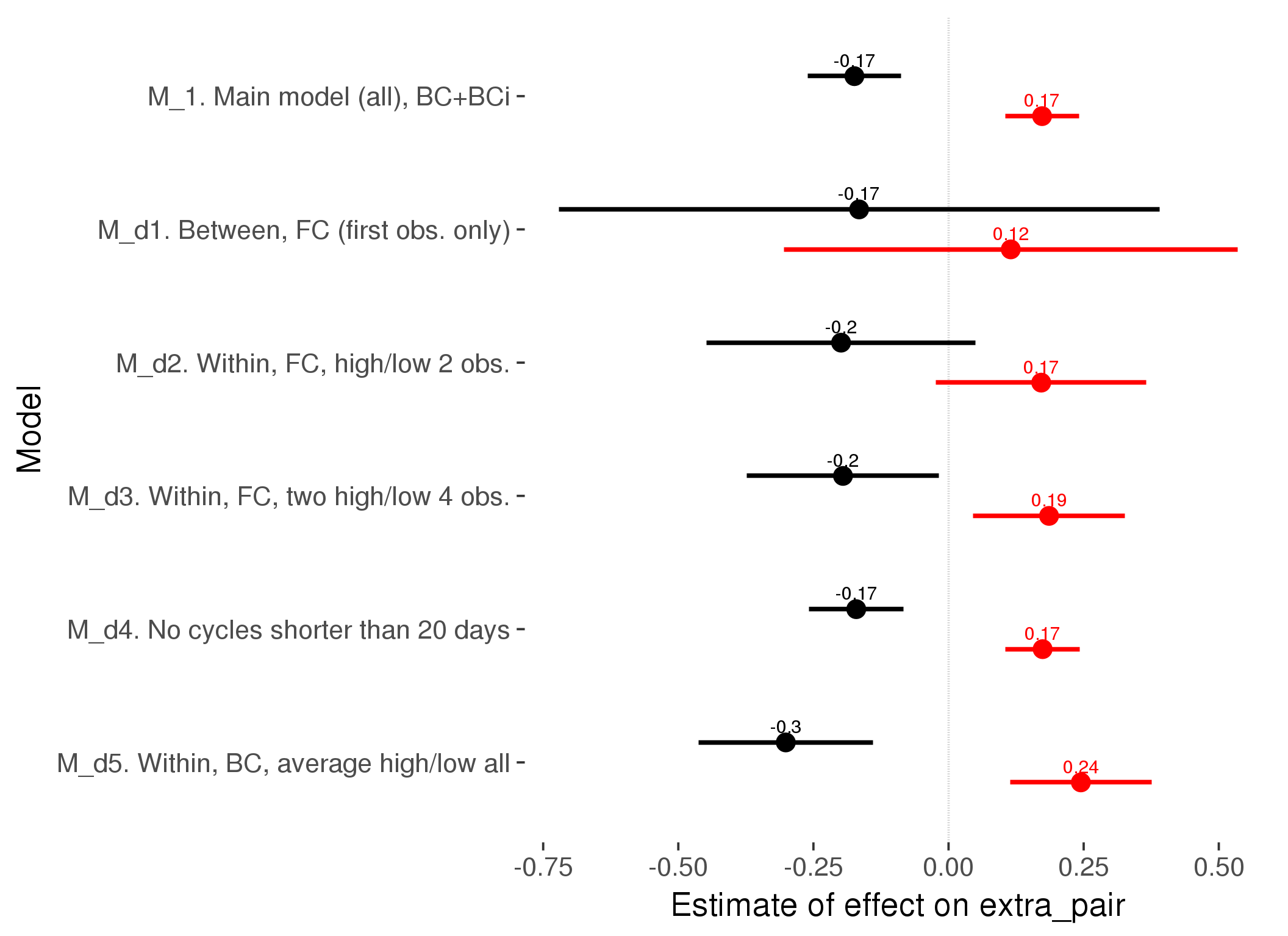
M_d: Other designs
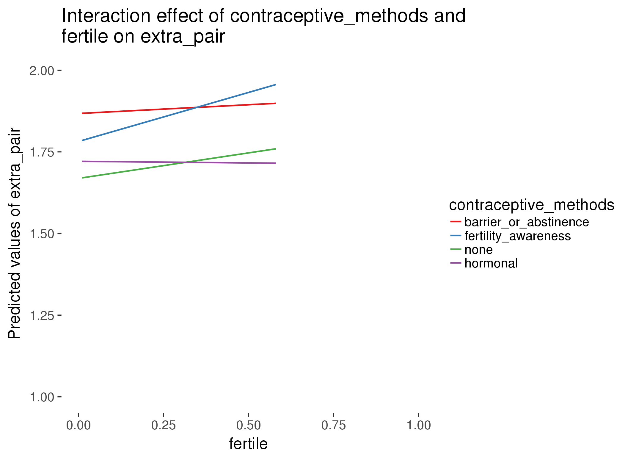
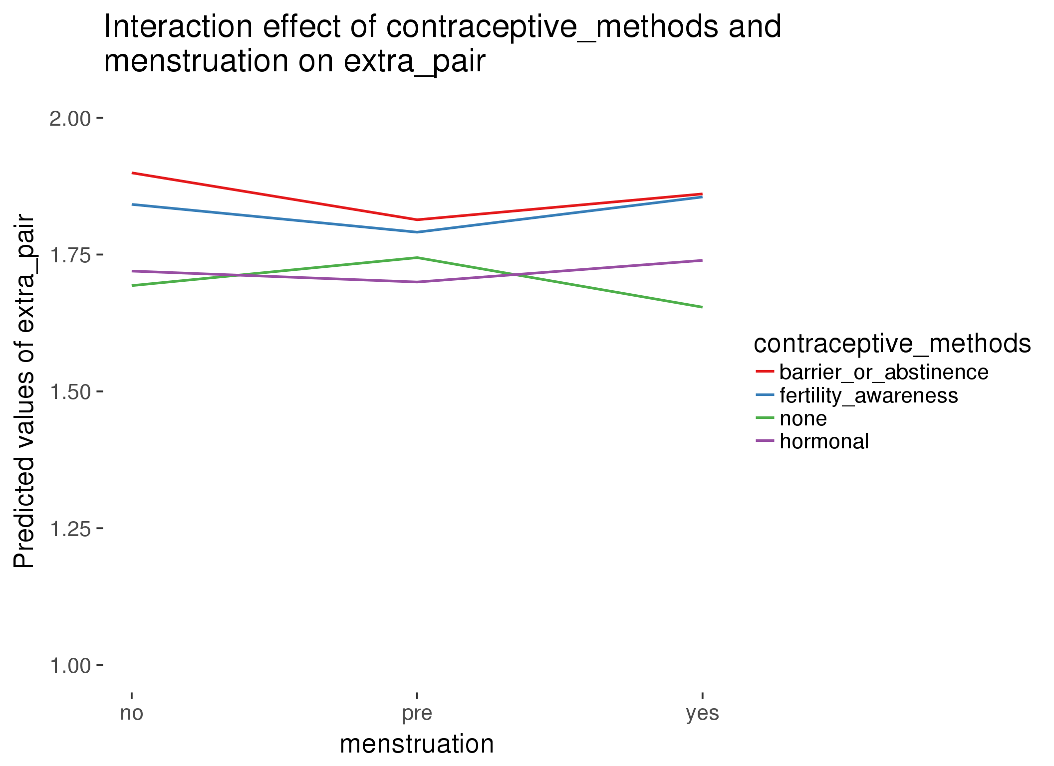
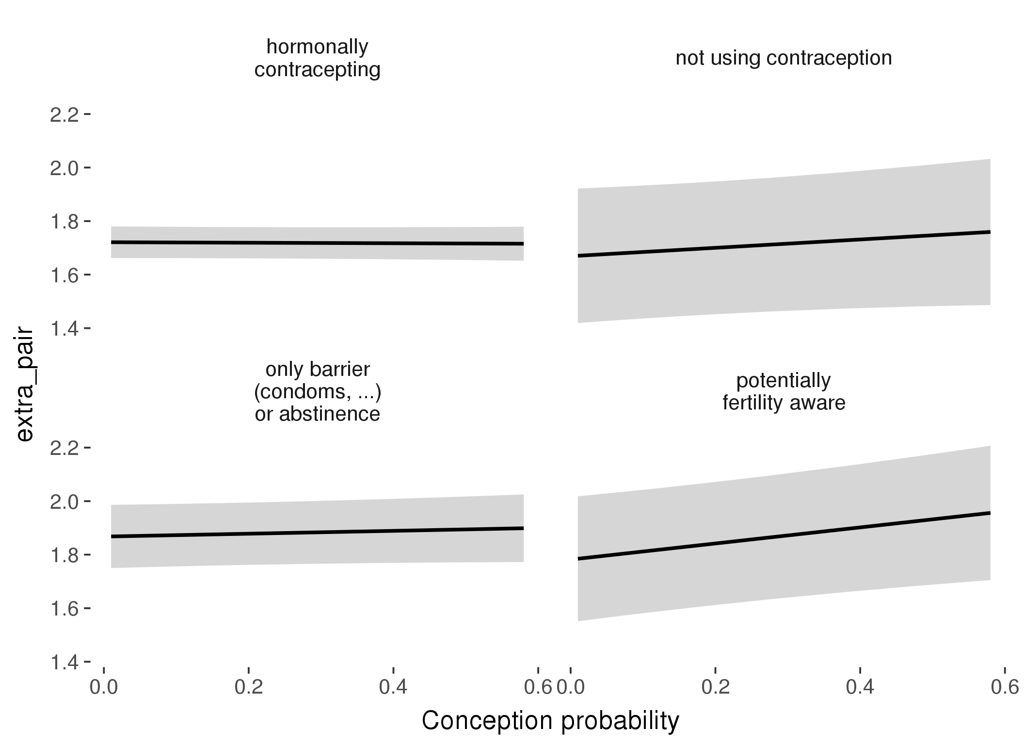
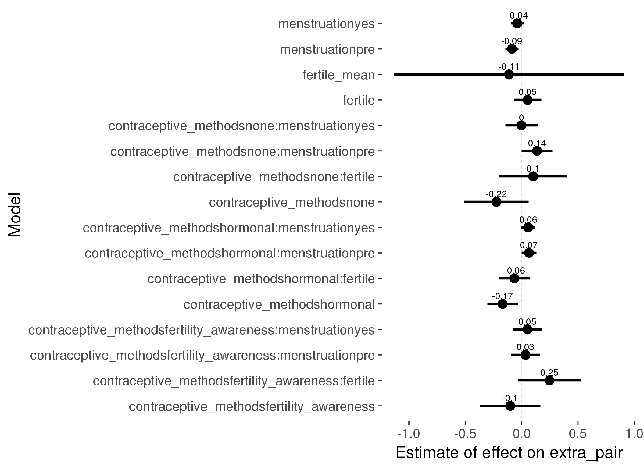
M_m1: Moderation by contraceptive method
Based on the sample with lax exclusion criteria. Users who used any hormonal contraception are classified as hormonal, users who use any awareness-based methods (counting, temperature-based) are classified as ‘fertility-awareness’, women who don’t fall into the before groups and use condoms, pessars, coitus interruptus etc. are classified as ‘barrie or abstinence’. Women who don’t use contraception or use other methods such as sterilisation are excluded from this analysis.
Linear mixed model fit by REML ['lmerMod']
Formula: extra_pair ~ fertile_mean + (1 | person) + contraceptive_methods +
    fertile + menstruation + fertile:contraceptive_methods +      menstruation:contraceptive_methods
   Data: diary
 Subset: !is.na(included_lax) & contraceptive_method != "other"

REML criterion at convergence: 30418

Scaled residuals:
   Min     1Q Median     3Q    Max
-4.348 -0.557 -0.148  0.408  8.097

Random effects:
 Groups   Name        Variance Std.Dev.
 person   (Intercept) 0.320    0.566
 Residual             0.313    0.560
Number of obs: 17026, groups:  person, 513

Fixed effects:
                                                          Estimate Std. Error t value
(Intercept)                                               1.909422   0.106971   17.85
fertile_mean                                             -0.111294   0.522029   -0.21
contraceptive_methodsfertility_awareness                 -0.100940   0.137287   -0.74
contraceptive_methodsnone                                -0.224004   0.145421   -1.54
contraceptive_methodshormonal                            -0.168364   0.069287   -2.43
fertile                                                   0.053678   0.062481    0.86
menstruationpre                                          -0.085755   0.030170   -2.84
menstruationyes                                          -0.038498   0.028824   -1.34
contraceptive_methodsfertility_awareness:fertile          0.246743   0.141881    1.74
contraceptive_methodsnone:fertile                         0.102445   0.153584    0.67
contraceptive_methodshormonal:fertile                    -0.063479   0.069805   -0.91
contraceptive_methodsfertility_awareness:menstruationpre  0.034951   0.066824    0.52
contraceptive_methodsnone:menstruationpre                 0.136851   0.069882    1.96
contraceptive_methodshormonal:menstruationpre             0.065769   0.033986    1.94
contraceptive_methodsfertility_awareness:menstruationyes  0.052088   0.067166    0.78
contraceptive_methodsnone:menstruationyes                -0.000944   0.073064   -0.01
contraceptive_methodshormonal:menstruationyes             0.058055   0.032875    1.77
refitting model(s) with ML (instead of REML)
| Df | AIC | BIC | logLik | deviance | Chisq | Chi Df | Pr(>Chisq) | |
|---|---|---|---|---|---|---|---|---|
| add_main | 13 | 30386 | 30486 | -15180 | 30360 | NA | NA | NA |
| by_method | 19 | 30390 | 30537 | -15176 | 30352 | 7.983 | 6 | 0.2393 |
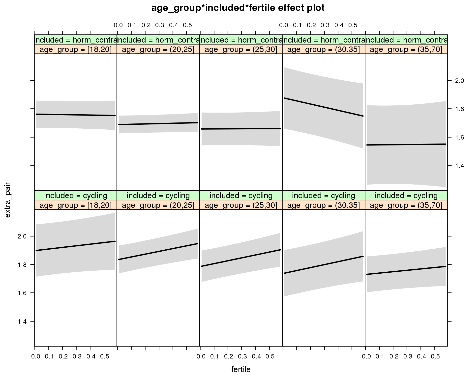
M_m2: Moderation by participant age
model %>%
  test_moderator("age_group", diary, xlevels = 5)
refitting model(s) with ML (instead of REML)
| Df | AIC | BIC | logLik | deviance | Chisq | Chi Df | Pr(>Chisq) | |
|---|---|---|---|---|---|---|---|---|
| with_main | 19 | 48529 | 48685 | -24246 | 48491 | NA | NA | NA |
| with_mod | 27 | 48538 | 48759 | -24242 | 48484 | 7.088 | 8 | 0.5271 |
Linear mixed model fit by REML ['lmerMod']
Formula: extra_pair ~ menstruation + fertile_mean + (1 | person) + age_group +
    included + fertile + menstruation:included + age_group:included +
    age_group:fertile + included:fertile + age_group:included:fertile
   Data: diary

REML criterion at convergence: 48582

Scaled residuals:
   Min     1Q Median     3Q    Max
-4.291 -0.558 -0.150  0.403  8.014

Random effects:
 Groups   Name        Variance Std.Dev.
 person   (Intercept) 0.312    0.558
 Residual             0.320    0.566
Number of obs: 26680, groups:  person, 1054

Fixed effects:
                                             Estimate Std. Error t value
(Intercept)                                   1.93884    0.09945   19.50
menstruationpre                              -0.09068    0.01730   -5.24
menstruationyes                              -0.07085    0.01632   -4.34
fertile_mean                                 -0.06982    0.21501   -0.32
age_group(20,25]                             -0.06427    0.10683   -0.60
age_group(25,30]                             -0.11225    0.10994   -1.02
age_group(30,35]                             -0.16170    0.12618   -1.28
age_group(35,70]                             -0.16834    0.11428   -1.47
includedhorm_contra                          -0.16358    0.10693   -1.53
fertile                                       0.11427    0.09980    1.14
menstruationpre:includedhorm_contra           0.06902    0.02221    3.11
menstruationyes:includedhorm_contra           0.08532    0.02139    3.99
age_group(20,25]:includedhorm_contra         -0.00928    0.12193   -0.08
age_group(25,30]:includedhorm_contra          0.00784    0.13421    0.06
age_group(30,35]:includedhorm_contra          0.27792    0.17496    1.59
age_group(35,70]:includedhorm_contra         -0.04939    0.19007   -0.26
age_group(20,25]:fertile                      0.08241    0.11058    0.75
age_group(25,30]:fertile                      0.08950    0.11397    0.79
age_group(30,35]:fertile                      0.09521    0.13203    0.72
age_group(35,70]:fertile                     -0.01630    0.11912   -0.14
includedhorm_contra:fertile                  -0.13051    0.11070   -1.18
age_group(20,25]:includedhorm_contra:fertile -0.04290    0.12387   -0.35
age_group(25,30]:includedhorm_contra:fertile -0.06894    0.13727   -0.50
age_group(30,35]:includedhorm_contra:fertile -0.30204    0.17720   -1.70
age_group(35,70]:includedhorm_contra:fertile  0.04258    0.20127    0.21
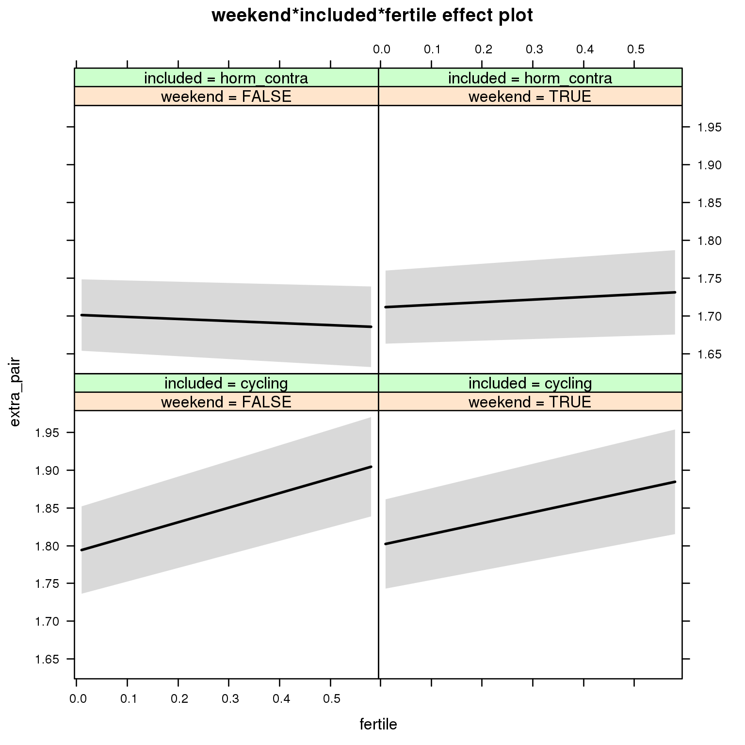
M_m3: Moderation by weekend
model %>%
  test_moderator("weekend", diary, xlevels = 2)
refitting model(s) with ML (instead of REML)
| Df | AIC | BIC | logLik | deviance | Chisq | Chi Df | Pr(>Chisq) | |
|---|---|---|---|---|---|---|---|---|
| with_main | 13 | 48521 | 48627 | -24247 | 48495 | NA | NA | NA |
| with_mod | 15 | 48522 | 48645 | -24246 | 48492 | 2.498 | 2 | 0.2868 |
Linear mixed model fit by REML ['lmerMod']
Formula: extra_pair ~ menstruation + fertile_mean + (1 | person) + weekend +
    included + fertile + menstruation:included + weekend:included +
    weekend:fertile + included:fertile + weekend:included:fertile
   Data: diary

REML criterion at convergence: 48564

Scaled residuals:
   Min     1Q Median     3Q    Max
-4.281 -0.558 -0.147  0.403  8.015

Random effects:
 Groups   Name        Variance Std.Dev.
 person   (Intercept) 0.311    0.558
 Residual             0.320    0.566
Number of obs: 26680, groups:  person, 1054

Fixed effects:
                                        Estimate Std. Error t value
(Intercept)                              1.83014    0.04737    38.6
menstruationpre                         -0.09047    0.01730    -5.2
menstruationyes                         -0.07133    0.01630    -4.4
fertile_mean                            -0.05361    0.21407    -0.3
weekendTRUE                              0.00853    0.01506     0.6
includedhorm_contra                     -0.11819    0.03936    -3.0
fertile                                  0.19329    0.04245     4.6
menstruationpre:includedhorm_contra      0.06887    0.02221     3.1
menstruationyes:includedhorm_contra      0.08598    0.02137     4.0
weekendTRUE:includedhorm_contra          0.00138    0.01939     0.1
weekendTRUE:fertile                     -0.04901    0.05842    -0.8
includedhorm_contra:fertile             -0.22048    0.05396    -4.1
weekendTRUE:includedhorm_contra:fertile  0.11050    0.07431     1.5
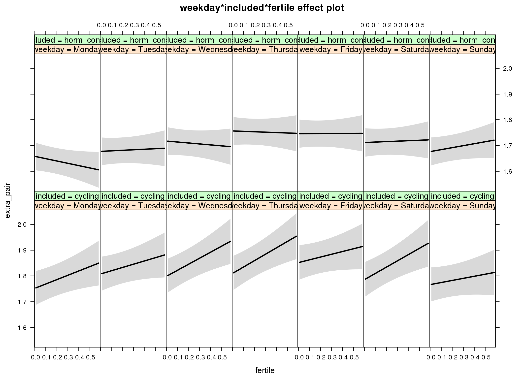
M_m4: Moderation by weekday
model %>%
  test_moderator("weekday", diary, xlevels = 7)
refitting model(s) with ML (instead of REML)
| Df | AIC | BIC | logLik | deviance | Chisq | Chi Df | Pr(>Chisq) | |
|---|---|---|---|---|---|---|---|---|
| with_main | 23 | 48449 | 48637 | -24201 | 48403 | NA | NA | NA |
| with_mod | 35 | 48463 | 48750 | -24196 | 48393 | 9.71 | 12 | 0.6414 |
Linear mixed model fit by REML ['lmerMod']
Formula: extra_pair ~ menstruation + fertile_mean + (1 | person) + weekday +
    included + fertile + menstruation:included + weekday:included +
    weekday:fertile + included:fertile + weekday:included:fertile
   Data: diary

REML criterion at convergence: 48559

Scaled residuals:
   Min     1Q Median     3Q    Max
-4.271 -0.556 -0.146  0.401  8.109

Random effects:
 Groups   Name        Variance Std.Dev.
 person   (Intercept) 0.311    0.558
 Residual             0.319    0.565
Number of obs: 26680, groups:  person, 1054

Fixed effects:
                                             Estimate Std. Error t value
(Intercept)                                   1.78818    0.05011    35.7
menstruationpre                              -0.09011    0.01727    -5.2
menstruationyes                              -0.07092    0.01628    -4.4
fertile_mean                                 -0.04487    0.21399    -0.2
weekdayTuesday                                0.05583    0.02691     2.1
weekdayWednesday                              0.04687    0.02687     1.7
weekdayThursday                               0.05778    0.02717     2.1
weekdayFriday                                 0.09984    0.02763     3.6
weekdaySaturday                               0.03339    0.02791     1.2
weekdaySunday                                 0.01445    0.02697     0.5
includedhorm_contra                          -0.12066    0.04459    -2.7
fertile                                       0.16868    0.07581     2.2
menstruationpre:includedhorm_contra           0.06754    0.02217     3.0
menstruationyes:includedhorm_contra           0.08425    0.02134     3.9
weekdayTuesday:includedhorm_contra           -0.03651    0.03457    -1.1
weekdayWednesday:includedhorm_contra          0.01248    0.03469     0.4
weekdayThursday:includedhorm_contra           0.04092    0.03502     1.2
weekdayFriday:includedhorm_contra            -0.01177    0.03550    -0.3
weekdaySaturday:includedhorm_contra           0.02035    0.03591     0.6
weekdaySunday:includedhorm_contra             0.00398    0.03481     0.1
weekdayTuesday:fertile                       -0.04163    0.10435    -0.4
weekdayWednesday:fertile                      0.06512    0.10483     0.6
weekdayThursday:fertile                       0.08043    0.10634     0.8
weekdayFriday:fertile                        -0.06118    0.10651    -0.6
weekdaySaturday:fertile                       0.07491    0.10793     0.7
weekdaySunday:fertile                        -0.08792    0.10489    -0.8
includedhorm_contra:fertile                  -0.25876    0.09698    -2.7
weekdayTuesday:includedhorm_contra:fertile    0.15258    0.13318     1.1
weekdayWednesday:includedhorm_contra:fertile -0.01241    0.13423    -0.1
weekdayThursday:includedhorm_contra:fertile  -0.00634    0.13533     0.0
weekdayFriday:includedhorm_contra:fertile     0.15357    0.13573     1.1
weekdaySaturday:includedhorm_contra:fertile   0.03271    0.13768     0.2
weekdaySunday:includedhorm_contra:fertile     0.25461    0.13398     1.9
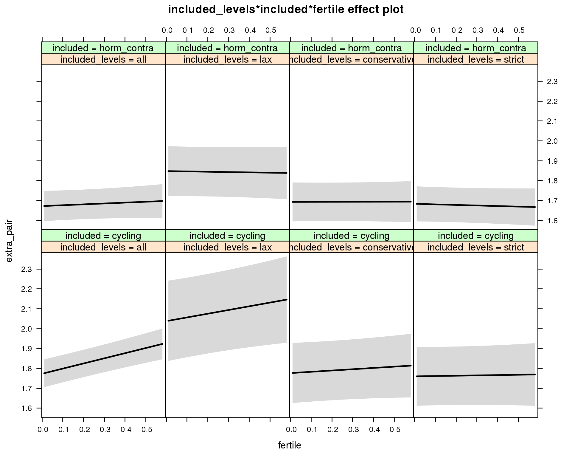
M_m5: Moderation by exclusion threshold
model %>%
  test_moderator("included_levels", diary, xlevels = 4)
refitting model(s) with ML (instead of REML)
| Df | AIC | BIC | logLik | deviance | Chisq | Chi Df | Pr(>Chisq) | |
|---|---|---|---|---|---|---|---|---|
| with_main | 17 | 48521 | 48661 | -24244 | 48487 | NA | NA | NA |
| with_mod | 23 | 48520 | 48708 | -24237 | 48474 | 13.28 | 6 | 0.03882 |
Linear mixed model fit by REML ['lmerMod']
Formula: extra_pair ~ menstruation + fertile_mean + (1 | person) + included_levels +
    included + fertile + menstruation:included + included_levels:included +
    included_levels:fertile + included:fertile + included_levels:included:fertile
   Data: diary

REML criterion at convergence: 48564

Scaled residuals:
   Min     1Q Median     3Q    Max
-4.295 -0.557 -0.149  0.405  7.997

Random effects:
 Groups   Name        Variance Std.Dev.
 person   (Intercept) 0.309    0.556
 Residual             0.320    0.566
Number of obs: 26680, groups:  person, 1054

Fixed effects:
                                                        Estimate Std. Error t value
(Intercept)                                               1.8208     0.0520    35.0
menstruationpre                                          -0.0929     0.0173    -5.4
menstruationyes                                          -0.0726     0.0163    -4.5
fertile_mean                                             -0.1052     0.2150    -0.5
included_levelslax                                        0.2646     0.1091     2.4
included_levelsconservative                               0.0033     0.0851     0.0
included_levelsstrict                                    -0.0132     0.0838    -0.2
includedhorm_contra                                      -0.1287     0.0537    -2.4
fertile                                                   0.2588     0.0441     5.9
menstruationpre:includedhorm_contra                       0.0707     0.0222     3.2
menstruationyes:includedhorm_contra                       0.0863     0.0214     4.0
included_levelslax:includedhorm_contra                   -0.0887     0.1326    -0.7
included_levelsconservative:includedhorm_contra           0.0177     0.1061     0.2
included_levelsstrict:includedhorm_contra                 0.0245     0.1027     0.2
included_levelslax:fertile                               -0.0720     0.1077    -0.7
included_levelsconservative:fertile                      -0.1942     0.0804    -2.4
included_levelsstrict:fertile                            -0.2427     0.0805    -3.0
includedhorm_contra:fertile                              -0.2152     0.0675    -3.2
included_levelslax:includedhorm_contra:fertile            0.0124     0.1315     0.1
included_levelsconservative:includedhorm_contra:fertile   0.1526     0.1047     1.5
included_levelsstrict:includedhorm_contra:fertile         0.1712     0.1031     1.7
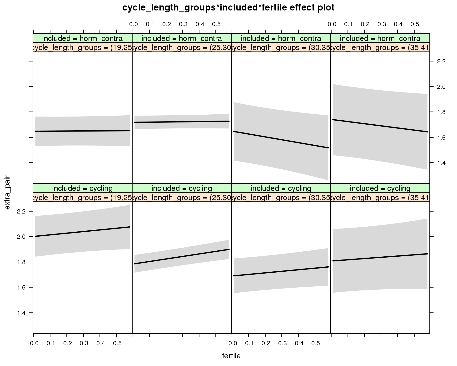
M_m6: Moderation by cycle length
model %>%
  test_moderator("cycle_length_groups", diary, xlevels = 4)
refitting model(s) with ML (instead of REML)
| Df | AIC | BIC | logLik | deviance | Chisq | Chi Df | Pr(>Chisq) | |
|---|---|---|---|---|---|---|---|---|
| with_main | 17 | 48523 | 48662 | -24245 | 48489 | NA | NA | NA |
| with_mod | 23 | 48529 | 48717 | -24241 | 48483 | 6.535 | 6 | 0.366 |
Linear mixed model fit by REML ['lmerMod']
Formula: extra_pair ~ menstruation + fertile_mean + (1 | person) + cycle_length_groups +
    included + fertile + menstruation:included + cycle_length_groups:included +
    cycle_length_groups:fertile + included:fertile + cycle_length_groups:included:fertile
   Data: diary

REML criterion at convergence: 48565

Scaled residuals:
   Min     1Q Median     3Q    Max
-4.315 -0.557 -0.147  0.405  8.013

Random effects:
 Groups   Name        Variance Std.Dev.
 person   (Intercept) 0.31     0.557
 Residual             0.32     0.566
Number of obs: 26680, groups:  person, 1054

Fixed effects:
                                                       Estimate Std. Error t value
(Intercept)                                              2.0444     0.0905   22.58
menstruationpre                                         -0.0898     0.0173   -5.18
menstruationyes                                         -0.0704     0.0164   -4.29
fertile_mean                                            -0.0900     0.2163   -0.42
cycle_length_groups(25,30]                              -0.2172     0.0892   -2.43
cycle_length_groups(30,35]                              -0.3113     0.1075   -2.90
cycle_length_groups(35,41]                              -0.1933     0.1522   -1.27
includedhorm_contra                                     -0.3802     0.1013   -3.75
fertile                                                  0.1292     0.0922    1.40
menstruationpre:includedhorm_contra                      0.0692     0.0222    3.11
menstruationyes:includedhorm_contra                      0.0859     0.0215    3.99
cycle_length_groups(25,30]:includedhorm_contra           0.2873     0.1102    2.61
cycle_length_groups(30,35]:includedhorm_contra           0.3122     0.1696    1.84
cycle_length_groups(35,41]:includedhorm_contra           0.2863     0.2165    1.32
cycle_length_groups(25,30]:fertile                       0.0698     0.0989    0.71
cycle_length_groups(30,35]:fertile                      -0.0060     0.1171   -0.05
cycle_length_groups(35,41]:fertile                      -0.0317     0.1654   -0.19
includedhorm_contra:fertile                             -0.1215     0.1088   -1.12
cycle_length_groups(25,30]:includedhorm_contra:fertile  -0.0625     0.1172   -0.53
cycle_length_groups(30,35]:includedhorm_contra:fertile  -0.2281     0.1843   -1.24
cycle_length_groups(35,41]:includedhorm_contra:fertile  -0.1442     0.2177   -0.66
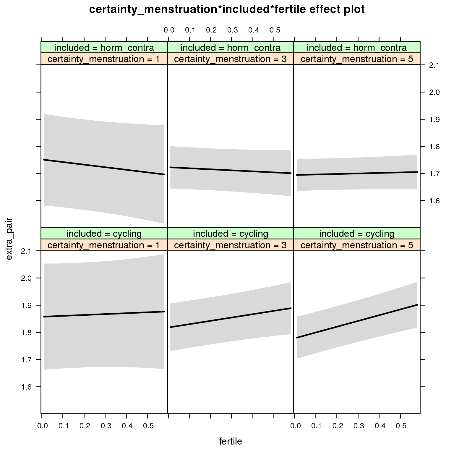
M_m7: Moderation by certainty about menstruation parameters
model %>%
  test_moderator("certainty_menstruation", diary)
refitting model(s) with ML (instead of REML)
| Df | AIC | BIC | logLik | deviance | Chisq | Chi Df | Pr(>Chisq) | |
|---|---|---|---|---|---|---|---|---|
| with_main | 13 | 48526 | 48632 | -24250 | 48500 | NA | NA | NA |
| with_mod | 15 | 48526 | 48649 | -24248 | 48496 | 3.154 | 2 | 0.2066 |
Linear mixed model fit by REML ['lmerMod']
Formula: extra_pair ~ menstruation + fertile_mean + (1 | person) + certainty_menstruation +
    included + fertile + menstruation:included + certainty_menstruation:included +
    certainty_menstruation:fertile + included:fertile + certainty_menstruation:included:fertile
   Data: diary

REML criterion at convergence: 48567

Scaled residuals:
   Min     1Q Median     3Q    Max
-4.283 -0.557 -0.149  0.405  8.005

Random effects:
 Groups   Name        Variance Std.Dev.
 person   (Intercept) 0.312    0.558
 Residual             0.320    0.566
Number of obs: 26680, groups:  person, 1054

Fixed effects:
                                                   Estimate Std. Error t value
(Intercept)                                         1.91365    0.13419   14.26
menstruationpre                                    -0.08973    0.01731   -5.18
menstruationyes                                    -0.07006    0.01633   -4.29
fertile_mean                                       -0.04686    0.21453   -0.22
certainty_menstruation                             -0.01977    0.03060   -0.65
includedhorm_contra                                -0.13841    0.17044   -0.81
fertile                                            -0.01189    0.13743   -0.09
menstruationpre:includedhorm_contra                 0.06836    0.02221    3.08
menstruationyes:includedhorm_contra                 0.08506    0.02140    3.98
certainty_menstruation:includedhorm_contra          0.00547    0.03972    0.14
certainty_menstruation:fertile                      0.04479    0.03220    1.39
includedhorm_contra:fertile                        -0.11161    0.17865   -0.62
certainty_menstruation:includedhorm_contra:fertile -0.01628    0.04129   -0.39
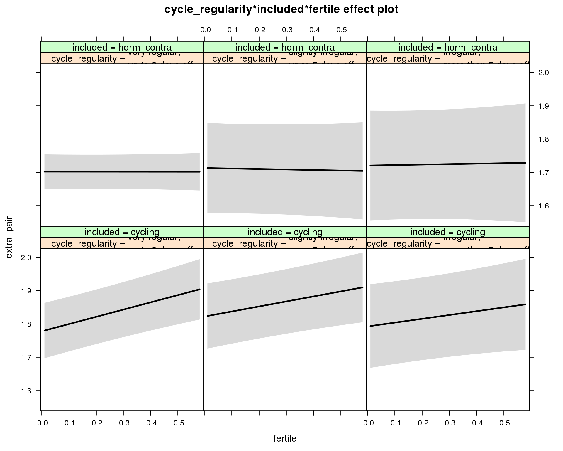
M_m8: Moderation by cycle regularity
model %>%
  test_moderator("cycle_regularity", diary)
refitting model(s) with ML (instead of REML)
| Df | AIC | BIC | logLik | deviance | Chisq | Chi Df | Pr(>Chisq) | |
|---|---|---|---|---|---|---|---|---|
| with_main | 15 | 48529 | 48652 | -24250 | 48499 | NA | NA | NA |
| with_mod | 19 | 48535 | 48691 | -24249 | 48497 | 1.985 | 4 | 0.7385 |
Linear mixed model fit by REML ['lmerMod']
Formula: extra_pair ~ menstruation + fertile_mean + (1 | person) + cycle_regularity +
    included + fertile + menstruation:included + cycle_regularity:included +
    cycle_regularity:fertile + included:fertile + cycle_regularity:included:fertile
   Data: diary

REML criterion at convergence: 48574

Scaled residuals:
   Min     1Q Median     3Q    Max
-4.286 -0.557 -0.148  0.405  8.010

Random effects:
 Groups   Name        Variance Std.Dev.
 person   (Intercept) 0.313    0.559
 Residual             0.320    0.566
Number of obs: 26680, groups:  person, 1054

Fixed effects:
                                                                                  Estimate Std. Error t value
(Intercept)                                                                        1.81624    0.05568    32.6
menstruationpre                                                                   -0.08972    0.01731    -5.2
menstruationyes                                                                   -0.07072    0.01631    -4.3
fertile_mean                                                                      -0.05723    0.21551    -0.3
cycle_regularityslightly irregular,\nup to 5 days off                              0.04439    0.06549     0.7
cycle_regularityirregular,\nmore than 5 days off                                   0.01462    0.07676     0.2
includedhorm_contra                                                               -0.10276    0.05096    -2.0
fertile                                                                            0.21712    0.04834     4.5
menstruationpre:includedhorm_contra                                                0.06826    0.02222     3.1
menstruationyes:includedhorm_contra                                                0.08518    0.02139     4.0
cycle_regularityslightly irregular,\nup to 5 days off:includedhorm_contra         -0.03353    0.09903    -0.3
cycle_regularityirregular,\nmore than 5 days off:includedhorm_contra               0.00369    0.11691     0.0
cycle_regularityslightly irregular,\nup to 5 days off:fertile                     -0.06645    0.06670    -1.0
cycle_regularityirregular,\nmore than 5 days off:fertile                          -0.10303    0.08205    -1.3
includedhorm_contra:fertile                                                       -0.21766    0.05665    -3.8
cycle_regularityslightly irregular,\nup to 5 days off:includedhorm_contra:fertile  0.05207    0.09901     0.5
cycle_regularityirregular,\nmore than 5 days off:includedhorm_contra:fertile       0.11767    0.12247     1.0
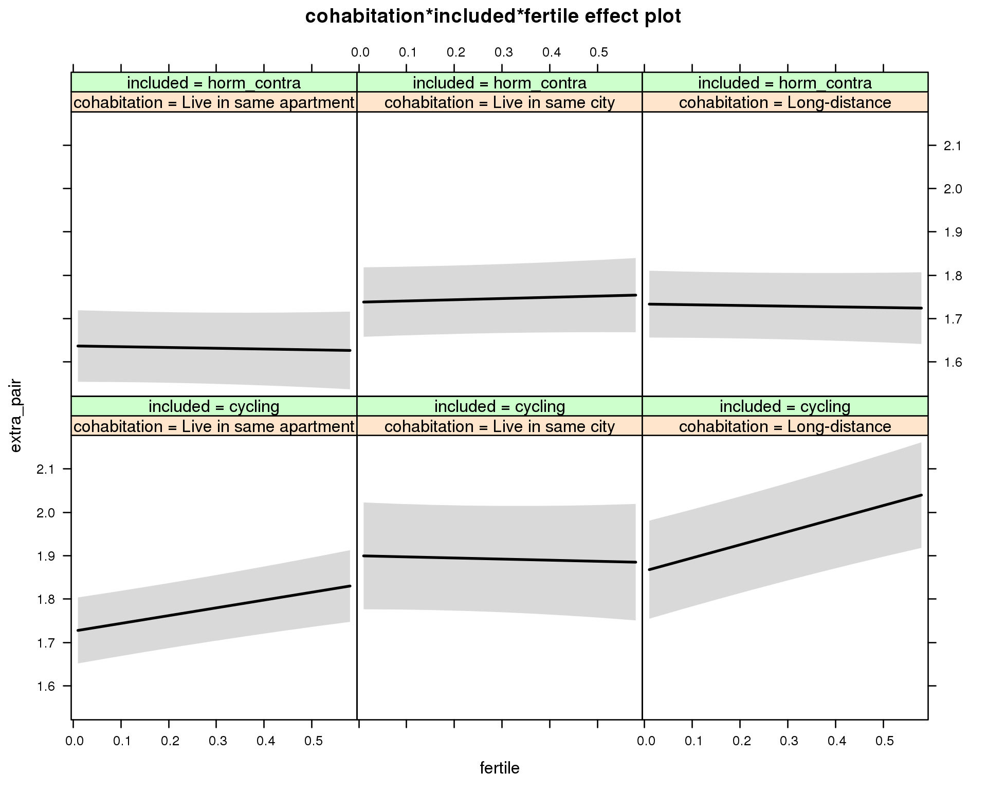
M_m9: Moderation by cohabitation status
model %>%
  test_moderator("cohabitation", diary)
refitting model(s) with ML (instead of REML)
| Df | AIC | BIC | logLik | deviance | Chisq | Chi Df | Pr(>Chisq) | |
|---|---|---|---|---|---|---|---|---|
| with_main | 15 | 48518 | 48641 | -24244 | 48488 | NA | NA | NA |
| with_mod | 19 | 48513 | 48668 | -24237 | 48475 | 13.7 | 4 | 0.008322 |
Linear mixed model fit by REML ['lmerMod']
Formula: extra_pair ~ menstruation + fertile_mean + (1 | person) + cohabitation +
    included + fertile + menstruation:included + cohabitation:included +
    cohabitation:fertile + included:fertile + cohabitation:included:fertile
   Data: diary

REML criterion at convergence: 48554

Scaled residuals:
   Min     1Q Median     3Q    Max
-4.283 -0.559 -0.148  0.401  8.003

Random effects:
 Groups   Name        Variance Std.Dev.
 person   (Intercept) 0.309    0.556
 Residual             0.320    0.566
Number of obs: 26680, groups:  person, 1054

Fixed effects:
                                                          Estimate Std. Error t value
(Intercept)                                                 1.7652     0.0537    32.9
menstruationpre                                            -0.0911     0.0173    -5.3
menstruationyes                                            -0.0726     0.0163    -4.5
fertile_mean                                               -0.0594     0.2138    -0.3
cohabitationLive in same city                               0.1739     0.0739     2.4
cohabitationLong-distance                                   0.1390     0.0696     2.0
includedhorm_contra                                        -0.1164     0.0581    -2.0
fertile                                                     0.1797     0.0436     4.1
menstruationpre:includedhorm_contra                         0.0694     0.0222     3.1
menstruationyes:includedhorm_contra                         0.0868     0.0214     4.1
cohabitationLive in same city:includedhorm_contra          -0.0730     0.0944    -0.8
cohabitationLong-distance:includedhorm_contra              -0.0424     0.0903    -0.5
cohabitationLive in same city:fertile                      -0.2051     0.0798    -2.6
cohabitationLong-distance:fertile                           0.1220     0.0718     1.7
includedhorm_contra:fertile                                -0.1976     0.0638    -3.1
cohabitationLive in same city:includedhorm_contra:fertile   0.2510     0.0997     2.5
cohabitationLong-distance:includedhorm_contra:fertile      -0.1201     0.0925    -1.3
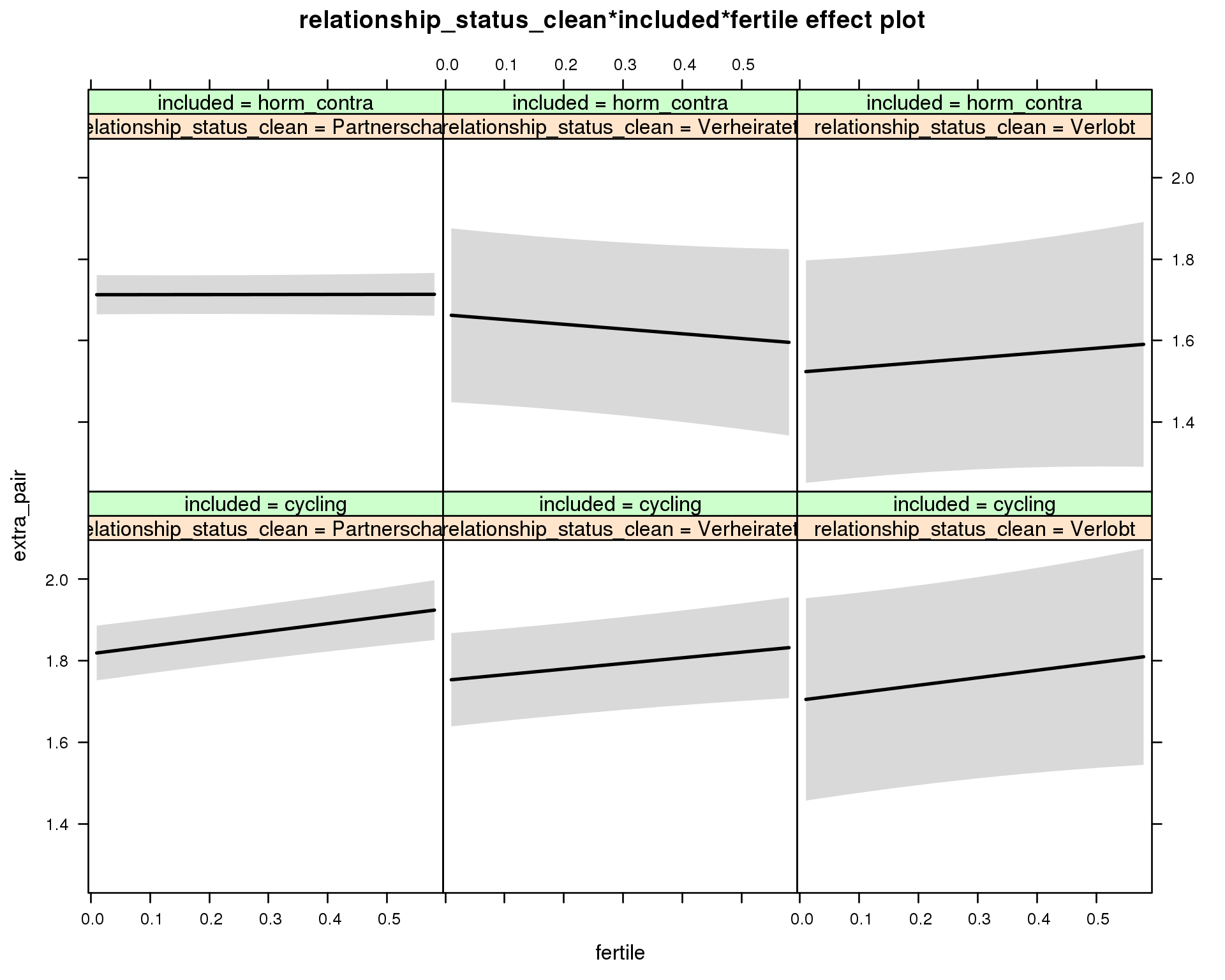
M_m10: Moderation by relationship status
model %>%
  test_moderator("relationship_status_clean", diary)
refitting model(s) with ML (instead of REML)
| Df | AIC | BIC | logLik | deviance | Chisq | Chi Df | Pr(>Chisq) | |
|---|---|---|---|---|---|---|---|---|
| with_main | 15 | 48526 | 48649 | -24248 | 48496 | NA | NA | NA |
| with_mod | 19 | 48532 | 48688 | -24247 | 48494 | 2.144 | 4 | 0.7094 |
Linear mixed model fit by REML ['lmerMod']
Formula: extra_pair ~ menstruation + fertile_mean + (1 | person) + relationship_status_clean +
    included + fertile + menstruation:included + relationship_status_clean:included +
    relationship_status_clean:fertile + included:fertile + relationship_status_clean:included:fertile
   Data: diary

REML criterion at convergence: 48564

Scaled residuals:
   Min     1Q Median     3Q    Max
-4.286 -0.557 -0.148  0.404  8.007

Random effects:
 Groups   Name        Variance Std.Dev.
 person   (Intercept) 0.311    0.558
 Residual             0.320    0.566
Number of obs: 26680, groups:  person, 1054

Fixed effects:
                                                                 Estimate Std. Error t value
(Intercept)                                                       1.85781    0.05042    36.8
menstruationpre                                                  -0.09044    0.01730    -5.2
menstruationyes                                                  -0.07123    0.01631    -4.4
fertile_mean                                                     -0.06836    0.21431    -0.3
relationship_status_cleanVerheiratet                             -0.06524    0.06768    -1.0
relationship_status_cleanVerlobt                                 -0.11395    0.13136    -0.9
includedhorm_contra                                              -0.13205    0.04333    -3.0
fertile                                                           0.18451    0.03998     4.6
menstruationpre:includedhorm_contra                               0.06911    0.02221     3.1
menstruationyes:includedhorm_contra                               0.08593    0.02138     4.0
relationship_status_cleanVerheiratet:includedhorm_contra          0.01591    0.13060     0.1
relationship_status_cleanVerlobt:includedhorm_contra             -0.07588    0.19324    -0.4
relationship_status_cleanVerheiratet:fertile                     -0.04634    0.07039    -0.7
relationship_status_cleanVerlobt:fertile                         -0.00095    0.13203     0.0
includedhorm_contra:fertile                                      -0.18286    0.04875    -3.8
relationship_status_cleanVerheiratet:includedhorm_contra:fertile -0.07167    0.13255    -0.5
relationship_status_cleanVerlobt:includedhorm_contra:fertile      0.11659    0.20500     0.6
do_moderators(models$extra_pair, diary)Moderators
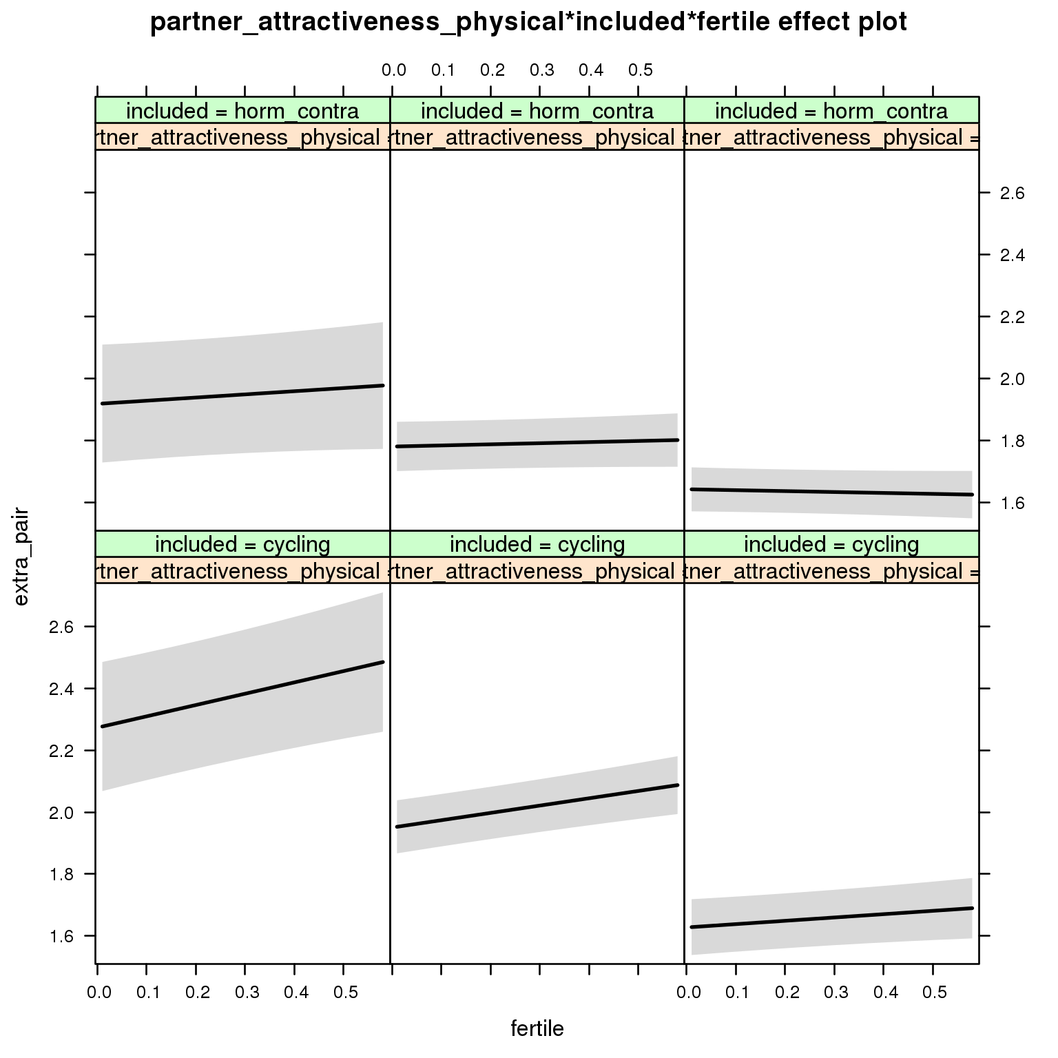
Partner’s physical attractiveness
Predicted fertile phase effect sizes (in red): biggest (EP desire, partner mate retention)/smallest (IP desire) when partner’s physical attractiveness is low.
model %>%
  test_moderator("partner_attractiveness_physical", diary)
refitting model(s) with ML (instead of REML)
| Df | AIC | BIC | logLik | deviance | Chisq | Chi Df | Pr(>Chisq) | |
|---|---|---|---|---|---|---|---|---|
| with_main | 13 | 48494 | 48601 | -24234 | 48468 | NA | NA | NA |
| with_mod | 15 | 48494 | 48617 | -24232 | 48464 | 4.093 | 2 | 0.1292 |
Linear mixed model fit by REML ['lmerMod']
Formula: extra_pair ~ menstruation + fertile_mean + (1 | person) + partner_attractiveness_physical +
    included + fertile + menstruation:included + partner_attractiveness_physical:included +
    partner_attractiveness_physical:fertile + included:fertile +
    partner_attractiveness_physical:included:fertile
   Data: diary

REML criterion at convergence: 48539

Scaled residuals:
   Min     1Q Median     3Q    Max
-4.283 -0.556 -0.148  0.406  8.003

Random effects:
 Groups   Name        Variance Std.Dev.
 person   (Intercept) 0.303    0.550
 Residual             0.320    0.566
Number of obs: 26680, groups:  person, 1054

Fixed effects:
                                                            Estimate Std. Error t value
(Intercept)                                                   2.4697     0.1448   17.06
menstruationpre                                              -0.0903     0.0173   -5.22
menstruationyes                                              -0.0714     0.0163   -4.38
fertile_mean                                                 -0.0379     0.2117   -0.18
partner_attractiveness_physical                              -0.0807     0.0174   -4.65
includedhorm_contra                                          -0.4750     0.1897   -2.50
fertile                                                       0.4299     0.1524    2.82
menstruationpre:includedhorm_contra                           0.0691     0.0222    3.11
menstruationyes:includedhorm_contra                           0.0861     0.0214    4.03
partner_attractiveness_physical:includedhorm_contra           0.0462     0.0231    2.00
partner_attractiveness_physical:fertile                      -0.0323     0.0187   -1.73
includedhorm_contra:fertile                                  -0.2947     0.2016   -1.46
partner_attractiveness_physical:includedhorm_contra:fertile   0.0158     0.0244    0.65
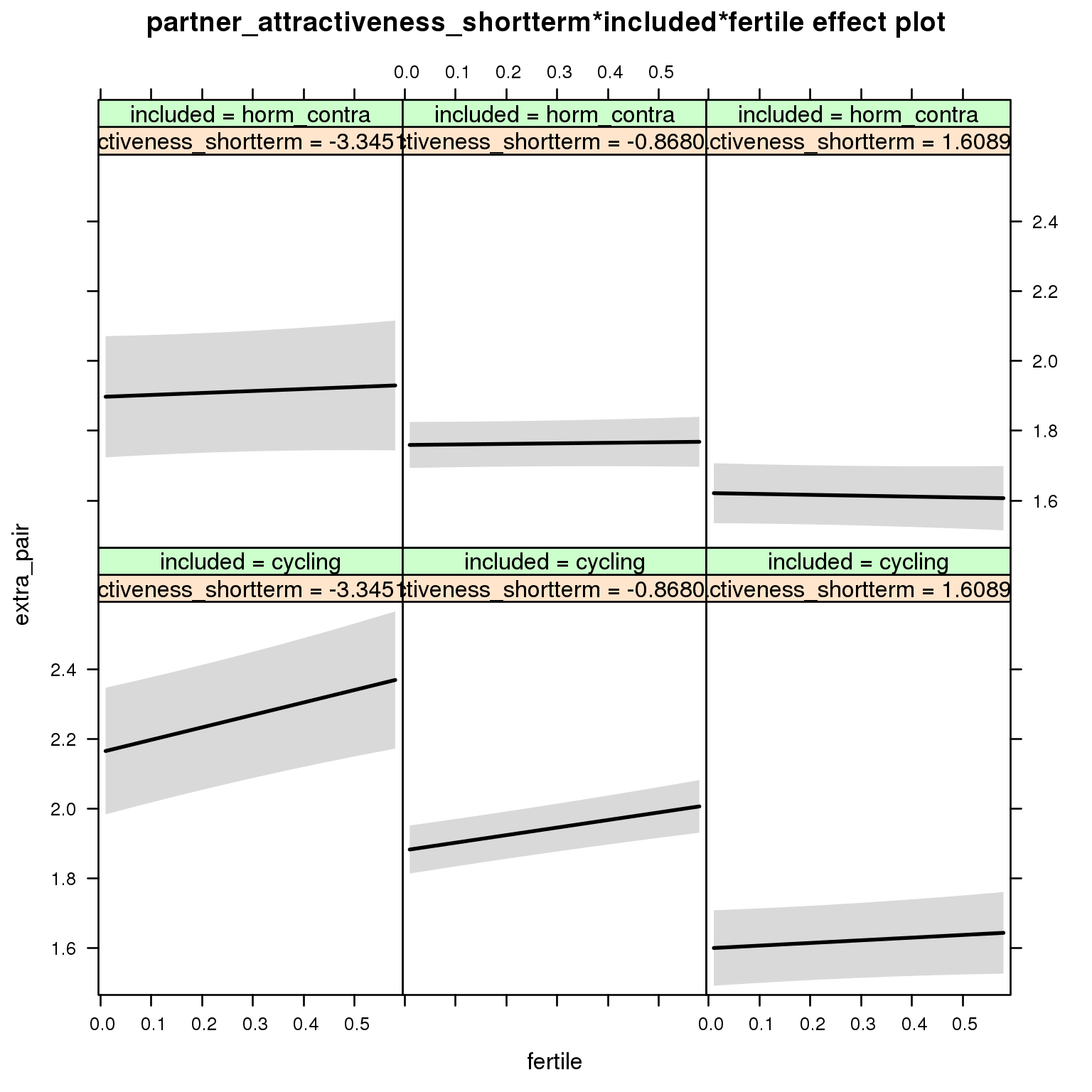
Partner’s short-term attractiveness
Predicted fertile phase effect sizes (in red): biggest (EP desire, partner mate retention)/smallest (IP desire) when partner’s short-term attractiveness is low.
model %>%
  test_moderator("partner_attractiveness_shortterm", diary)
refitting model(s) with ML (instead of REML)
| Df | AIC | BIC | logLik | deviance | Chisq | Chi Df | Pr(>Chisq) | |
|---|---|---|---|---|---|---|---|---|
| with_main | 13 | 48499 | 48606 | -24237 | 48473 | NA | NA | NA |
| with_mod | 15 | 48499 | 48622 | -24235 | 48469 | 4.184 | 2 | 0.1234 |
Linear mixed model fit by REML ['lmerMod']
Formula: extra_pair ~ menstruation + fertile_mean + (1 | person) + partner_attractiveness_shortterm +
    included + fertile + menstruation:included + partner_attractiveness_shortterm:included +
    partner_attractiveness_shortterm:fertile + included:fertile +
    partner_attractiveness_shortterm:included:fertile
   Data: diary

REML criterion at convergence: 48540

Scaled residuals:
   Min     1Q Median     3Q    Max
-4.286 -0.556 -0.148  0.404  8.006

Random effects:
 Groups   Name        Variance Std.Dev.
 person   (Intercept) 0.305    0.552
 Residual             0.320    0.566
Number of obs: 26680, groups:  person, 1054

Fixed effects:
                                                             Estimate Std. Error t value
(Intercept)                                                    1.8176     0.0467    38.9
menstruationpre                                               -0.0905     0.0173    -5.2
menstruationyes                                               -0.0715     0.0163    -4.4
fertile_mean                                                  -0.0393     0.2123    -0.2
partner_attractiveness_shortterm                              -0.1135     0.0274    -4.1
includedhorm_contra                                           -0.0987     0.0384    -2.6
fertile                                                        0.1676     0.0350     4.8
menstruationpre:includedhorm_contra                            0.0692     0.0222     3.1
menstruationyes:includedhorm_contra                            0.0862     0.0214     4.0
partner_attractiveness_shortterm:includedhorm_contra           0.0578     0.0369     1.6
partner_attractiveness_shortterm:fertile                      -0.0567     0.0293    -1.9
includedhorm_contra:fertile                                   -0.1662     0.0445    -3.7
partner_attractiveness_shortterm:includedhorm_contra:fertile   0.0402     0.0384     1.0
Partner’s short-term vs. long-term attractiveness
Predicted fertile phase effect sizes (in red): biggest (EP desire, partner mate retention)/smallest (IP desire) top-right (high LT, low ST), then top-left (low LT, low ST), then bottom-left (low LT, high ST), then bottom-right (high LT/ST).
add_main = update.formula(formula(model), new = as.formula(paste0(". ~ . + partner_attractiveness_longterm * included + partner_attractiveness_shortterm * included + partner_attractiveness_longterm * partner_attractiveness_shortterm"))) # reorder so that the triptych looks nice
add_mod_formula = update.formula(update.formula(formula(model), new = . ~ . - included * fertile), new = as.formula(paste0(". ~ . + partner_attractiveness_longterm * fertile * partner_attractiveness_shortterm * included"))) # reorder so that the triptych looks nice

update(model, formula = add_main) -> with_main
update(model, formula = add_mod_formula) -> with_mod
cat(pander(anova(with_main, with_mod)))
refitting model(s) with ML (instead of REML)
| Df | AIC | BIC | logLik | deviance | Chisq | Chi Df | Pr(>Chisq) | |
|---|---|---|---|---|---|---|---|---|
| with_main | 16 | 48448 | 48579 | -24208 | 48416 | NA | NA | NA |
| with_mod | 23 | 48446 | 48634 | -24200 | 48400 | 15.96 | 7 | 0.02553 |
effs = allEffects(with_mod)
effs = data.frame(effs$`partner_attractiveness_longterm:fertile:partner_attractiveness_shortterm:included`) %>%
  filter(partner_attractiveness_longterm %in% c(-2,0),partner_attractiveness_shortterm %in% c(-2,0))
ggplot(effs, aes(fertile, fit, ymin = lower, ymax = upper, color = included)) +
  facet_grid(partner_attractiveness_shortterm ~ partner_attractiveness_longterm) +
  geom_smooth(stat='identity') +
  scale_color_manual(values = c("cycling" = 'red', 'horm_contra' = 'black'), guide = F) +
  scale_fill_manual(values = c("cycling" = 'red', 'horm_contra' = 'black'), guide = F) +
  ggtitle("Moderation", "top-to-bottom: short-term,\nleft-to-right: long-term attractiveness of the partner")+
  ylab(names(model@frame)[1])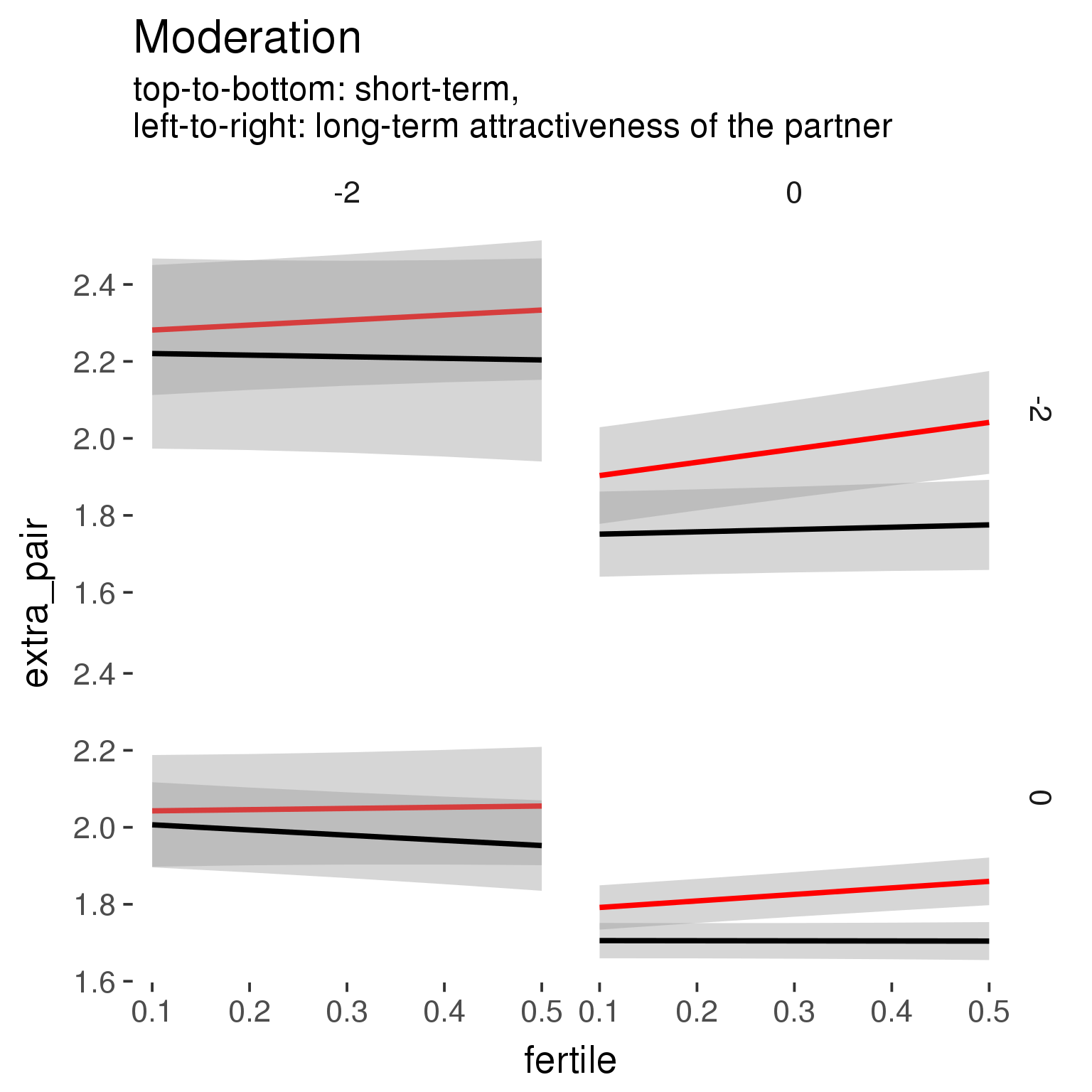
print_summary(with_mod)Linear mixed model fit by REML ['lmerMod']
Formula: extra_pair ~ menstruation + fertile_mean + (1 | person) + partner_attractiveness_longterm +
fertile + partner_attractiveness_shortterm + included + menstruation:included +
partner_attractiveness_longterm:fertile + partner_attractiveness_longterm:partner_attractiveness_shortterm +
fertile:partner_attractiveness_shortterm + partner_attractiveness_longterm:included +
fertile:included + partner_attractiveness_shortterm:included +
partner_attractiveness_longterm:fertile:partner_attractiveness_shortterm +
partner_attractiveness_longterm:fertile:included + partner_attractiveness_longterm:partner_attractiveness_shortterm:included +
fertile:partner_attractiveness_shortterm:included + partner_attractiveness_longterm:fertile:partner_attractiveness_shortterm:included
Data: diary
REML criterion at convergence: 48514
Scaled residuals:
Min 1Q Median 3Q Max
-4.285 -0.557 -0.148 0.403 7.987
Random effects:
Groups Name Variance Std.Dev.
person (Intercept) 0.289 0.537
Residual 0.320 0.566
Number of obs: 26680, groups: person, 1054
Fixed effects:
Estimate
(Intercept) 1.81689
menstruationpre -0.08939
menstruationyes -0.06950
fertile_mean -0.08072
partner_attractiveness_longterm -0.13238
fertile 0.16947
partner_attractiveness_shortterm -0.04705
includedhorm_contra -0.09586
menstruationpre:includedhorm_contra 0.06851
menstruationyes:includedhorm_contra 0.08475
partner_attractiveness_longterm:fertile 0.06901
partner_attractiveness_longterm:partner_attractiveness_shortterm 0.03371
fertile:partner_attractiveness_shortterm -0.08784
partner_attractiveness_longterm:includedhorm_contra -0.02470
fertile:includedhorm_contra -0.17245
partner_attractiveness_shortterm:includedhorm_contra 0.02739
partner_attractiveness_longterm:fertile:partner_attractiveness_shortterm -0.01932
partner_attractiveness_longterm:fertile:includedhorm_contra -0.00301
partner_attractiveness_longterm:partner_attractiveness_shortterm:includedhorm_contra 0.00761
fertile:partner_attractiveness_shortterm:includedhorm_contra 0.05629
partner_attractiveness_longterm:fertile:partner_attractiveness_shortterm:includedhorm_contra 0.02688
Std. Error
(Intercept) 0.04690
menstruationpre 0.01729
menstruationyes 0.01632
fertile_mean 0.20816
partner_attractiveness_longterm 0.03233
fertile 0.03654
partner_attractiveness_shortterm 0.02979
includedhorm_contra 0.03937
menstruationpre:includedhorm_contra 0.02220
menstruationyes:includedhorm_contra 0.02138
partner_attractiveness_longterm:fertile 0.03534
partner_attractiveness_longterm:partner_attractiveness_shortterm 0.02380
fertile:partner_attractiveness_shortterm 0.03203
partner_attractiveness_longterm:includedhorm_contra 0.04123
fertile:includedhorm_contra 0.04607
partner_attractiveness_shortterm:includedhorm_contra 0.03886
partner_attractiveness_longterm:fertile:partner_attractiveness_shortterm 0.02617
partner_attractiveness_longterm:fertile:includedhorm_contra 0.04481
partner_attractiveness_longterm:partner_attractiveness_shortterm:includedhorm_contra 0.03716
fertile:partner_attractiveness_shortterm:includedhorm_contra 0.04106
partner_attractiveness_longterm:fertile:partner_attractiveness_shortterm:includedhorm_contra 0.04051
t value
(Intercept) 38.7
menstruationpre -5.2
menstruationyes -4.3
fertile_mean -0.4
partner_attractiveness_longterm -4.1
fertile 4.6
partner_attractiveness_shortterm -1.6
includedhorm_contra -2.4
menstruationpre:includedhorm_contra 3.1
menstruationyes:includedhorm_contra 4.0
partner_attractiveness_longterm:fertile 2.0
partner_attractiveness_longterm:partner_attractiveness_shortterm 1.4
fertile:partner_attractiveness_shortterm -2.7
partner_attractiveness_longterm:includedhorm_contra -0.6
fertile:includedhorm_contra -3.7
partner_attractiveness_shortterm:includedhorm_contra 0.7
partner_attractiveness_longterm:fertile:partner_attractiveness_shortterm -0.7
partner_attractiveness_longterm:fertile:includedhorm_contra -0.1
partner_attractiveness_longterm:partner_attractiveness_shortterm:includedhorm_contra 0.2
fertile:partner_attractiveness_shortterm:includedhorm_contra 1.4
partner_attractiveness_longterm:fertile:partner_attractiveness_shortterm:includedhorm_contra 0.7
Relative attractiveness to self
whole MV and MV_P scale
Predicted fertile phase effect sizes (in red): biggest (EP desire, partner mate retention)/smallest (IP desire) when partner’s relative attractiveness is low.
three item subsets of the MV/MV_P scale
model %>%
  test_moderator("partner_attractiveness_rel_to_self_MV_short", diary)
refitting model(s) with ML (instead of REML)
| Df | AIC | BIC | logLik | deviance | Chisq | Chi Df | Pr(>Chisq) | |
|---|---|---|---|---|---|---|---|---|
| with_main | 13 | 48525 | 48632 | -24250 | 48499 | NA | NA | NA |
| with_mod | 15 | 48528 | 48651 | -24249 | 48498 | 1.305 | 2 | 0.5207 |
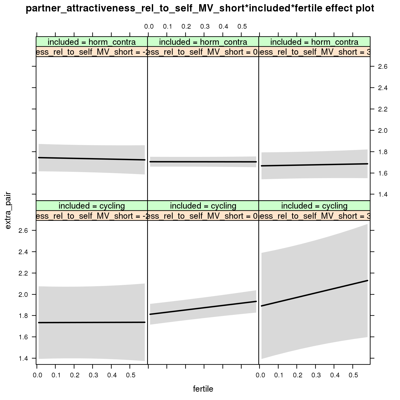
Linear mixed model fit by REML ['lmerMod']
Formula:
extra_pair ~ menstruation + fertile_mean + (1 | person) + partner_attractiveness_rel_to_self_MV_short +
    included + fertile + menstruation:included + partner_attractiveness_rel_to_self_MV_short:included +
    partner_attractiveness_rel_to_self_MV_short:fertile + included:fertile +
    partner_attractiveness_rel_to_self_MV_short:included:fertile
   Data: diary

REML criterion at convergence: 48567

Scaled residuals:
   Min     1Q Median     3Q    Max
-4.291 -0.557 -0.149  0.404  8.014

Random effects:
 Groups   Name        Variance Std.Dev.
 person   (Intercept) 0.312    0.558
 Residual             0.320    0.566
Number of obs: 26680, groups:  person, 1054

Fixed effects:
                                                                        Estimate Std. Error t value
(Intercept)                                                               1.8428     0.0529    34.8
menstruationpre                                                          -0.0905     0.0173    -5.2
menstruationyes                                                          -0.0709     0.0163    -4.3
fertile_mean                                                             -0.0579     0.2143    -0.3
partner_attractiveness_rel_to_self_MV_short                               0.0243     0.0678     0.4
includedhorm_contra                                                      -0.1229     0.0454    -2.7
fertile                                                                   0.1950     0.0415     4.7
menstruationpre:includedhorm_contra                                       0.0690     0.0222     3.1
menstruationyes:includedhorm_contra                                       0.0852     0.0214     4.0
partner_attractiveness_rel_to_self_MV_short:includedhorm_contra          -0.0368     0.0705    -0.5
partner_attractiveness_rel_to_self_MV_short:fertile                       0.0659     0.0675     1.0
includedhorm_contra:fertile                                              -0.1996     0.0500    -4.0
partner_attractiveness_rel_to_self_MV_short:includedhorm_contra:fertile  -0.0547     0.0701    -0.8
model %>%
  test_moderator("partner_attractiveness_rel_to_self", diary)
refitting model(s) with ML (instead of REML)
| Df | AIC | BIC | logLik | deviance | Chisq | Chi Df | Pr(>Chisq) | |
|---|---|---|---|---|---|---|---|---|
| with_main | 13 | 48525 | 48632 | -24250 | 48499 | NA | NA | NA |
| with_mod | 15 | 48528 | 48651 | -24249 | 48498 | 0.9981 | 2 | 0.6071 |
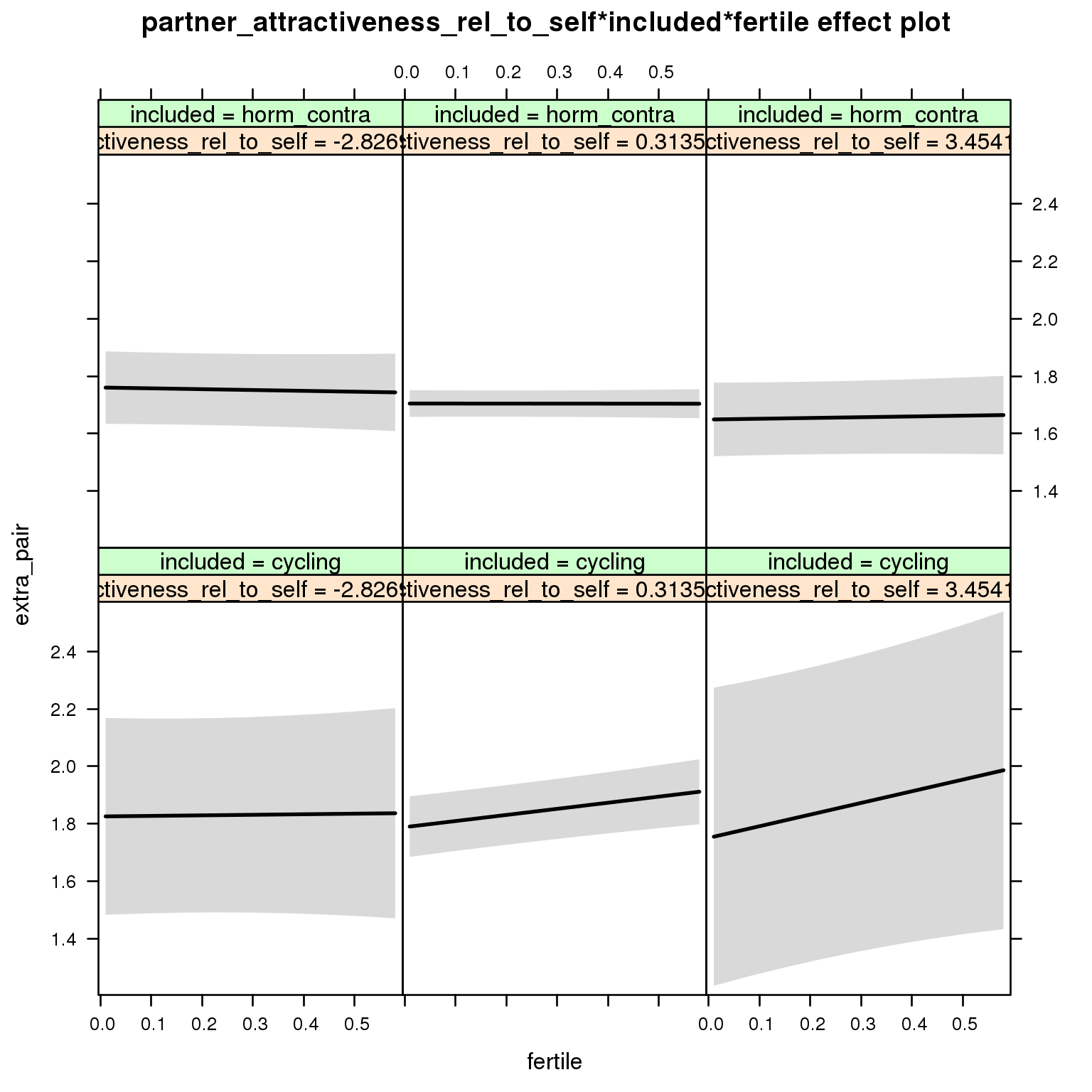
Linear mixed model fit by REML ['lmerMod']
Formula: extra_pair ~ menstruation + fertile_mean + (1 | person) + partner_attractiveness_rel_to_self +
    included + fertile + menstruation:included + partner_attractiveness_rel_to_self:included +
    partner_attractiveness_rel_to_self:fertile + included:fertile +
    partner_attractiveness_rel_to_self:included:fertile
   Data: diary

REML criterion at convergence: 48567

Scaled residuals:
   Min     1Q Median     3Q    Max
-4.290 -0.557 -0.149  0.405  8.013

Random effects:
 Groups   Name        Variance Std.Dev.
 person   (Intercept) 0.312    0.558
 Residual             0.320    0.566
Number of obs: 26680, groups:  person, 1054

Fixed effects:
                                                               Estimate Std. Error t value
(Intercept)                                                     1.82982    0.05305    34.5
menstruationpre                                                -0.09049    0.01730    -5.2
menstruationyes                                                -0.07093    0.01631    -4.3
fertile_mean                                                   -0.05483    0.21424    -0.3
partner_attractiveness_rel_to_self                             -0.01187    0.06952    -0.2
includedhorm_contra                                            -0.10889    0.04558    -2.4
fertile                                                         0.19331    0.04179     4.6
menstruationpre:includedhorm_contra                             0.06900    0.02221     3.1
menstruationyes:includedhorm_contra                             0.08526    0.02138     4.0
partner_attractiveness_rel_to_self:includedhorm_contra         -0.00588    0.07215    -0.1
partner_attractiveness_rel_to_self:fertile                      0.06158    0.06986     0.9
includedhorm_contra:fertile                                    -0.19728    0.05021    -3.9
partner_attractiveness_rel_to_self:includedhorm_contra:fertile -0.05269    0.07237    -0.7
Partner’s shortterm attractiveness, alternative specification
model %>%
  test_moderator("partner_attractiveness_shortterm_v2", diary)
refitting model(s) with ML (instead of REML)
| Df | AIC | BIC | logLik | deviance | Chisq | Chi Df | Pr(>Chisq) | |
|---|---|---|---|---|---|---|---|---|
| with_main | 13 | 48502 | 48609 | -24238 | 48476 | NA | NA | NA |
| with_mod | 15 | 48504 | 48627 | -24237 | 48474 | 2.683 | 2 | 0.2614 |
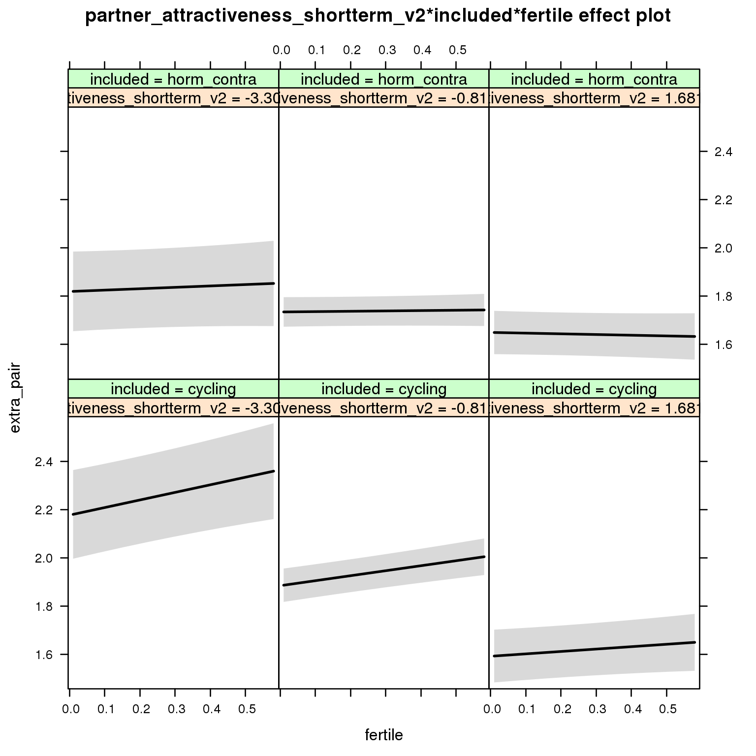
Linear mixed model fit by REML ['lmerMod']
Formula: extra_pair ~ menstruation + fertile_mean + (1 | person) + partner_attractiveness_shortterm_v2 +
    included + fertile + menstruation:included + partner_attractiveness_shortterm_v2:included +
    partner_attractiveness_shortterm_v2:fertile + included:fertile +
    partner_attractiveness_shortterm_v2:included:fertile
   Data: diary

REML criterion at convergence: 48545

Scaled residuals:
   Min     1Q Median     3Q    Max
-4.284 -0.556 -0.149  0.405  8.004

Random effects:
 Groups   Name        Variance Std.Dev.
 person   (Intercept) 0.305    0.552
 Residual             0.320    0.566
Number of obs: 26680, groups:  person, 1054

Fixed effects:
                                                                Estimate Std. Error t value
(Intercept)                                                       1.8219     0.0466    39.1
menstruationpre                                                  -0.0901     0.0173    -5.2
menstruationyes                                                  -0.0710     0.0163    -4.4
fertile_mean                                                     -0.0279     0.2124    -0.1
partner_attractiveness_shortterm_v2                              -0.1173     0.0276    -4.3
includedhorm_contra                                              -0.1095     0.0383    -2.9
fertile                                                           0.1719     0.0349     4.9
menstruationpre:includedhorm_contra                               0.0689     0.0222     3.1
menstruationyes:includedhorm_contra                               0.0857     0.0214     4.0
partner_attractiveness_shortterm_v2:includedhorm_contra           0.0833     0.0366     2.3
partner_attractiveness_shortterm_v2:fertile                      -0.0431     0.0292    -1.5
includedhorm_contra:fertile                                      -0.1717     0.0443    -3.9
partner_attractiveness_shortterm_v2:includedhorm_contra:fertile   0.0257     0.0380     0.7
Partner’s global attractiveness
model %>%
  test_moderator("partner_attractiveness_global", diary)
refitting model(s) with ML (instead of REML)
| Df | AIC | BIC | logLik | deviance | Chisq | Chi Df | Pr(>Chisq) | |
|---|---|---|---|---|---|---|---|---|
| with_main | 13 | 48522 | 48629 | -24248 | 48496 | NA | NA | NA |
| with_mod | 15 | 48525 | 48648 | -24248 | 48495 | 1.031 | 2 | 0.5971 |
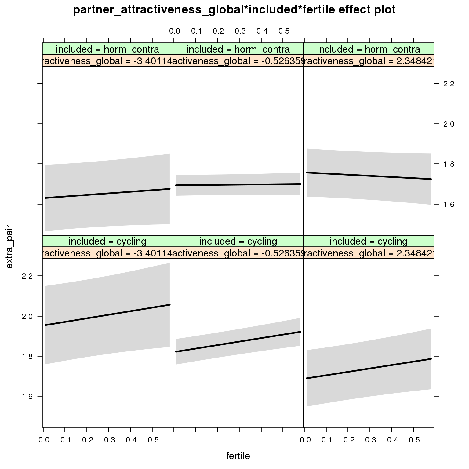
Linear mixed model fit by REML ['lmerMod']
Formula: extra_pair ~ menstruation + fertile_mean + (1 | person) + partner_attractiveness_global +
    included + fertile + menstruation:included + partner_attractiveness_global:included +
    partner_attractiveness_global:fertile + included:fertile +
    partner_attractiveness_global:included:fertile
   Data: diary

REML criterion at convergence: 48567

Scaled residuals:
   Min     1Q Median     3Q    Max
-4.287 -0.556 -0.149  0.405  8.009

Random effects:
 Groups   Name        Variance Std.Dev.
 person   (Intercept) 0.311    0.557
 Residual             0.320    0.566
Number of obs: 26680, groups:  person, 1054

Fixed effects:
                                                          Estimate Std. Error t value
(Intercept)                                                1.83307    0.04693    39.1
menstruationpre                                           -0.09042    0.01730    -5.2
menstruationyes                                           -0.07115    0.01631    -4.4
fertile_mean                                              -0.04867    0.21402    -0.2
partner_attractiveness_global                             -0.04613    0.02807    -1.6
includedhorm_contra                                       -0.11812    0.03852    -3.1
fertile                                                    0.17329    0.03491     5.0
menstruationpre:includedhorm_contra                        0.06921    0.02221     3.1
menstruationyes:includedhorm_contra                        0.08578    0.02138     4.0
partner_attractiveness_global:includedhorm_contra          0.06838    0.03686     1.9
partner_attractiveness_global:fertile                     -0.00137    0.02895     0.0
includedhorm_contra:fertile                               -0.17460    0.04425    -3.9
partner_attractiveness_global:includedhorm_contra:fertile -0.02232    0.03720    -0.6
Partner’s longterm attractiveness
model %>%
  test_moderator("partner_attractiveness_longterm", diary)
refitting model(s) with ML (instead of REML)
| Df | AIC | BIC | logLik | deviance | Chisq | Chi Df | Pr(>Chisq) | |
|---|---|---|---|---|---|---|---|---|
| with_main | 13 | 48452 | 48559 | -24213 | 48426 | NA | NA | NA |
| with_mod | 15 | 48449 | 48572 | -24210 | 48419 | 6.762 | 2 | 0.03401 |
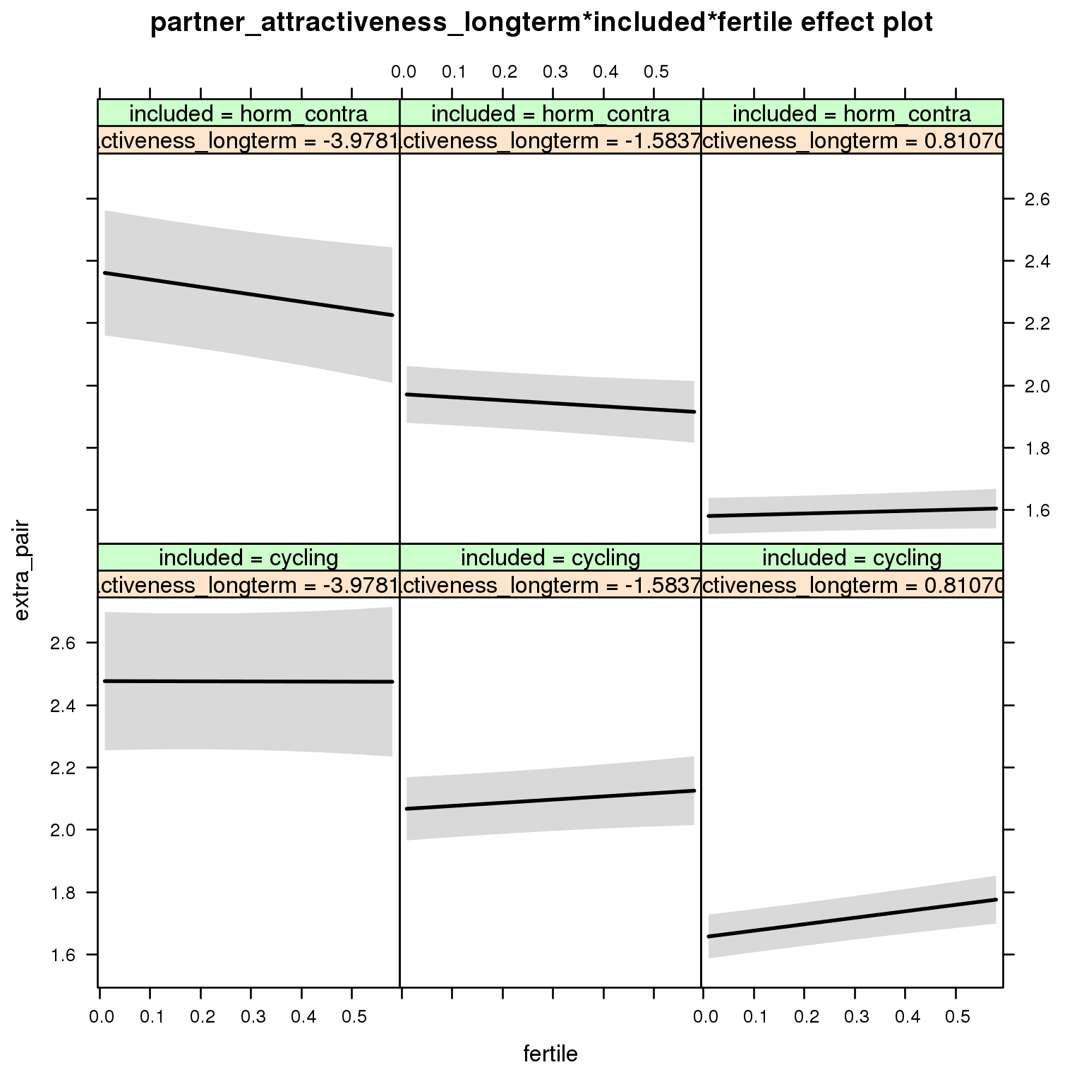
Linear mixed model fit by REML ['lmerMod']
Formula: extra_pair ~ menstruation + fertile_mean + (1 | person) + partner_attractiveness_longterm +
    included + fertile + menstruation:included + partner_attractiveness_longterm:included +
    partner_attractiveness_longterm:fertile + included:fertile +
    partner_attractiveness_longterm:included:fertile
   Data: diary

REML criterion at convergence: 48490

Scaled residuals:
   Min     1Q Median     3Q    Max
-4.298 -0.557 -0.148  0.403  7.997

Random effects:
 Groups   Name        Variance Std.Dev.
 person   (Intercept) 0.29     0.538
 Residual             0.32     0.566
Number of obs: 26680, groups:  person, 1054

Fixed effects:
                                                            Estimate Std. Error t value
(Intercept)                                                  1.84183    0.04562    40.4
menstruationpre                                             -0.08964    0.01729    -5.2
menstruationyes                                             -0.06976    0.01632    -4.3
fertile_mean                                                -0.11011    0.20832    -0.5
partner_attractiveness_longterm                             -0.17146    0.02766    -6.2
includedhorm_contra                                         -0.10852    0.03744    -2.9
fertile                                                      0.17152    0.03491     4.9
menstruationpre:includedhorm_contra                          0.06863    0.02220     3.1
menstruationyes:includedhorm_contra                          0.08497    0.02138     4.0
partner_attractiveness_longterm:includedhorm_contra          0.00807    0.03718     0.2
partner_attractiveness_longterm:fertile                      0.04400    0.03095     1.4
includedhorm_contra:fertile                                 -0.17694    0.04429    -4.0
partner_attractiveness_longterm:includedhorm_contra:fertile  0.01433    0.04094     0.3
Partner’s short-term vs. long-term attractiveness
We also test this specification of the short-term vs. long-term moderator prediction, but we think this is a suboptimal way to test it.
model %>%
  test_moderator("partner_st_vs_lt", diary)
refitting model(s) with ML (instead of REML)
| Df | AIC | BIC | logLik | deviance | Chisq | Chi Df | Pr(>Chisq) | |
|---|---|---|---|---|---|---|---|---|
| with_main | 13 | 48516 | 48622 | -24245 | 48490 | NA | NA | NA |
| with_mod | 15 | 48506 | 48629 | -24238 | 48476 | 13.93 | 2 | 0.000946 |
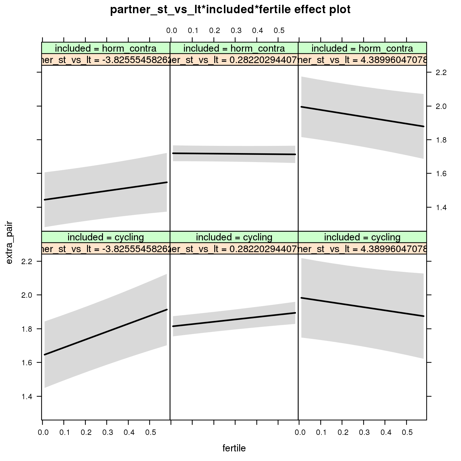
Linear mixed model fit by REML ['lmerMod']
Formula: extra_pair ~ menstruation + fertile_mean + (1 | person) + partner_st_vs_lt +
    included + fertile + menstruation:included + partner_st_vs_lt:included +
    partner_st_vs_lt:fertile + included:fertile + partner_st_vs_lt:included:fertile
   Data: diary

REML criterion at convergence: 48548

Scaled residuals:
   Min     1Q Median     3Q    Max
-4.268 -0.557 -0.148  0.405  7.979

Random effects:
 Groups   Name        Variance Std.Dev.
 person   (Intercept) 0.309    0.556
 Residual             0.320    0.566
Number of obs: 26680, groups:  person, 1054

Fixed effects:
                                             Estimate Std. Error t value
(Intercept)                                    1.8414     0.0470    39.2
menstruationpre                               -0.0901     0.0173    -5.2
menstruationyes                               -0.0704     0.0163    -4.3
fertile_mean                                  -0.0675     0.2136    -0.3
partner_st_vs_lt                               0.0418     0.0260     1.6
includedhorm_contra                           -0.1276     0.0385    -3.3
fertile                                        0.1620     0.0351     4.6
menstruationpre:includedhorm_contra            0.0690     0.0222     3.1
menstruationyes:includedhorm_contra            0.0851     0.0214     4.0
partner_st_vs_lt:includedhorm_contra           0.0257     0.0331     0.8
partner_st_vs_lt:fertile                      -0.0803     0.0270    -3.0
includedhorm_contra:fertile                   -0.1602     0.0444    -3.6
partner_st_vs_lt:includedhorm_contra:fertile   0.0333     0.0341     1.0
Partner’s mate value
long scale
model %>%
  test_moderator("MV_P", diary)
refitting model(s) with ML (instead of REML)
| Df | AIC | BIC | logLik | deviance | Chisq | Chi Df | Pr(>Chisq) | |
|---|---|---|---|---|---|---|---|---|
| with_main | 13 | 48523 | 48629 | -24248 | 48497 | NA | NA | NA |
| with_mod | 15 | 48526 | 48649 | -24248 | 48496 | 0.2159 | 2 | 0.8977 |
Error: Error in plot.eff(x[[(i - 1) * cols + j]], row = i, col = j, nrow = rows, : x.var = ‘fertile’ is not in the effect.
short scale
model %>%
  test_moderator("MV_P_short", diary)
refitting model(s) with ML (instead of REML)
| Df | AIC | BIC | logLik | deviance | Chisq | Chi Df | Pr(>Chisq) | |
|---|---|---|---|---|---|---|---|---|
| with_main | 13 | 48524 | 48631 | -24249 | 48498 | NA | NA | NA |
| with_mod | 15 | 48527 | 48650 | -24248 | 48497 | 1.837 | 2 | 0.3991 |
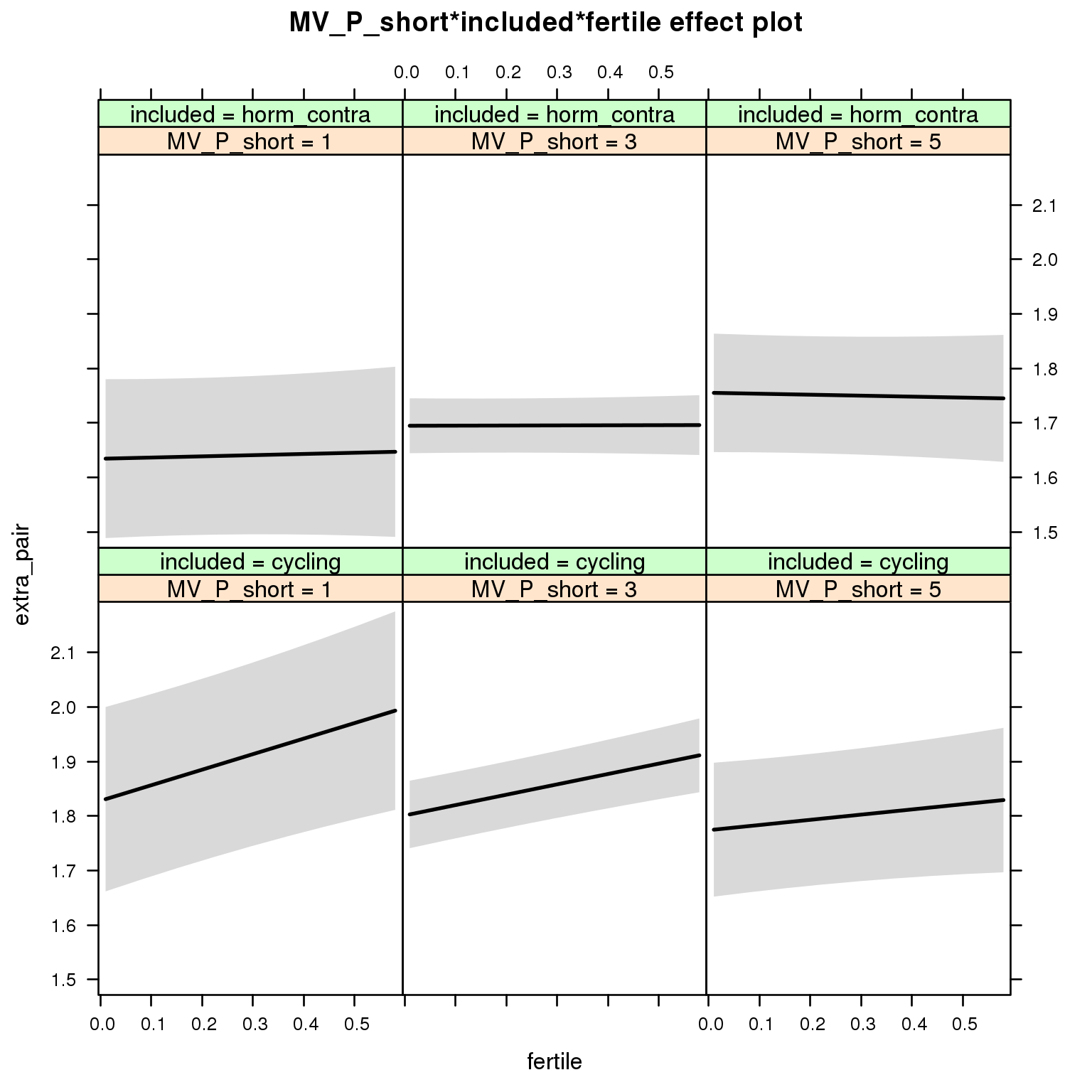
Linear mixed model fit by REML ['lmerMod']
Formula: extra_pair ~ menstruation + fertile_mean + (1 | person) + MV_P_short +
    included + fertile + menstruation:included + MV_P_short:included +
    MV_P_short:fertile + included:fertile + MV_P_short:included:fertile
   Data: diary

REML criterion at convergence: 48566

Scaled residuals:
   Min     1Q Median     3Q    Max
-4.284 -0.556 -0.149  0.405  8.007

Random effects:
 Groups   Name        Variance Std.Dev.
 person   (Intercept) 0.311    0.558
 Residual             0.320    0.566
Number of obs: 26680, groups:  person, 1054

Fixed effects:
                                       Estimate Std. Error t value
(Intercept)                              1.8801     0.1246   15.09
menstruationpre                         -0.0908     0.0173   -5.25
menstruationyes                         -0.0715     0.0163   -4.38
fertile_mean                            -0.0566     0.2141   -0.26
MV_P_short                              -0.0135     0.0343   -0.39
includedhorm_contra                     -0.2651     0.1583   -1.67
fertile                                  0.3326     0.1264    2.63
menstruationpre:includedhorm_contra      0.0694     0.0222    3.12
menstruationyes:includedhorm_contra      0.0860     0.0214    4.02
MV_P_short:includedhorm_contra           0.0438     0.0457    0.96
MV_P_short:fertile                      -0.0475     0.0361   -1.31
includedhorm_contra:fertile             -0.3007     0.1632   -1.84
MV_P_short:includedhorm_contra:fertile   0.0375     0.0469    0.80
Partner’s job and income
model %>%
  test_moderator("partner_attractiveness_money", diary)
refitting model(s) with ML (instead of REML)
| Df | AIC | BIC | logLik | deviance | Chisq | Chi Df | Pr(>Chisq) | |
|---|---|---|---|---|---|---|---|---|
| with_main | 13 | 48525 | 48632 | -24250 | 48499 | NA | NA | NA |
| with_mod | 15 | 48529 | 48652 | -24250 | 48499 | 0.2694 | 2 | 0.874 |
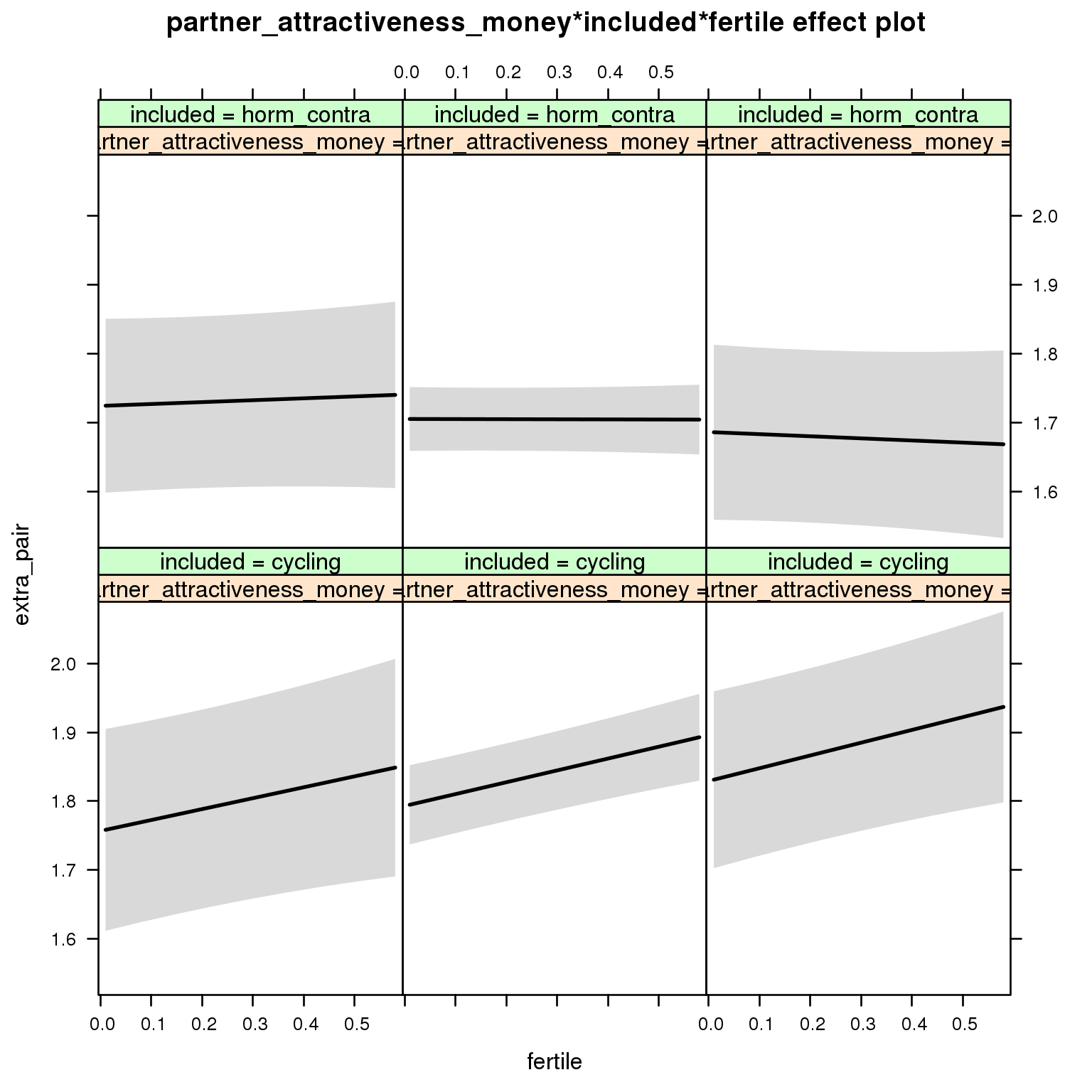
Linear mixed model fit by REML ['lmerMod']
Formula: extra_pair ~ menstruation + fertile_mean + (1 | person) + partner_attractiveness_money +
    included + fertile + menstruation:included + partner_attractiveness_money:included +
    partner_attractiveness_money:fertile + included:fertile +
    partner_attractiveness_money:included:fertile
   Data: diary

REML criterion at convergence: 48569

Scaled residuals:
   Min     1Q Median     3Q    Max
-4.286 -0.557 -0.150  0.405  8.004

Random effects:
 Groups   Name        Variance Std.Dev.
 person   (Intercept) 0.312    0.558
 Residual             0.320    0.566
Number of obs: 26680, groups:  person, 1054

Fixed effects:
                                                         Estimate Std. Error t value
(Intercept)                                               1.77559    0.11217   15.83
menstruationpre                                          -0.09049    0.01730   -5.23
menstruationyes                                          -0.07127    0.01631   -4.37
fertile_mean                                             -0.04849    0.21436   -0.23
partner_attractiveness_money                              0.01813    0.03199    0.57
includedhorm_contra                                      -0.03243    0.14080   -0.23
fertile                                                   0.15176    0.11108    1.37
menstruationpre:includedhorm_contra                       0.06905    0.02221    3.11
menstruationyes:includedhorm_contra                       0.08576    0.02138    4.01
partner_attractiveness_money:includedhorm_contra         -0.02762    0.04395   -0.63
partner_attractiveness_money:fertile                      0.00672    0.03324    0.20
includedhorm_contra:fertile                              -0.10970    0.14578   -0.75
partner_attractiveness_money:includedhorm_contra:fertile -0.02125    0.04504   -0.47
Specific robustness analyses for extra-pair effects
Just libido?
Does the effect on extra-pair desire remain after adjusting for the effect on in-pair desire and vice versa?
Yes, if anything they suppress one another’s effects, because they are negatively associated, but both positively associated with fertility. However, we unfortunately did not measure non-directed “libido” (e.g. irrespective of potential partner/solo), precluding any strong conclusions about the independence of these effects (see also here).
Models
lmer(extra_pair_desire ~ included * (fertile + menstruation) + fertile_mean + menstruation + (1 | person), data = diary) %->%
  m_extra_not_adjusted_for_in  %>%
  print_summary()  %>%
  plot_all_effects()
##
##
## ```
## Linear mixed model fit by REML
## t-tests use Satterthwaite approximations to degrees of freedom ['lmerMod']
## Formula: extra_pair_desire ~ included * (fertile + menstruation) + fertile_mean +
## menstruation + (1 | person)
## Data: diary
##
## REML criterion at convergence: 52397
##
## Scaled residuals:
## Min 1Q Median 3Q Max
## -4.866 -0.494 -0.129 0.331 7.409
##
## Random effects:
## Groups Name Variance Std.Dev.
## person (Intercept) 0.421 0.649
## Residual 0.368 0.607
## Number of obs: 26680, groups: person, 1054
##
## Fixed effects:
## Estimate Std. Error df t value Pr(>|t|)
## (Intercept) 1.8236 0.0538 1263.0000 33.88 < 2e-16 ***
## includedhorm_contra -0.2181 0.0443 1211.0000 -4.93 0.000000944176 ***
## fertile 0.2494 0.0374 25853.0000 6.66 0.000000000027 ***
## menstruationpre -0.1125 0.0185 25855.0000 -6.06 0.000000001341 ***
## menstruationyes -0.0778 0.0175 25944.0000 -4.45 0.000008585201 ***
## fertile_mean -0.2660 0.2447 1365.0000 -1.09 0.2772
## includedhorm_contra:fertile -0.2383 0.0474 25950.0000 -5.02 0.000000513140 ***
## includedhorm_contra:menstruationpre 0.0750 0.0238 25851.0000 3.15 0.0016 **
## includedhorm_contra:menstruationyes 0.0893 0.0229 25926.0000 3.90 0.000097428845 ***
## ---
## Signif. codes: 0 '***' 0.001 '**' 0.01 '*' 0.05 '.' 0.1 ' ' 1
##
## Correlation of Fixed Effects:
## (Intr) incld_ fertil mnstrtnp mnstrtny frtl_m inclddhrm_cntr:f
## inclddhrm_c -0.475
## fertile -0.126 0.207
## menstrutnpr -0.131 0.167 0.467
## menstrutnys -0.128 0.161 0.385 0.398
## fertile_men -0.771 -0.023 -0.056 -0.008 -0.005
## inclddhrm_cntr:f 0.126 -0.262 -0.787 -0.368 -0.304 0.009
## inclddhrm_cntr:mnstrtnp 0.108 -0.209 -0.363 -0.779 -0.310 -0.002 0.467
## inclddhrm_cntr:mnstrtny 0.103 -0.198 -0.293 -0.304 -0.763 -0.002 0.382
## inclddhrm_cntr:mnstrtnp
## inclddhrm_c
## fertile
## menstrutnpr
## menstrutnys
## fertile_men
## inclddhrm_cntr:f
## inclddhrm_cntr:mnstrtnp
## inclddhrm_cntr:mnstrtny 0.384
##
## ```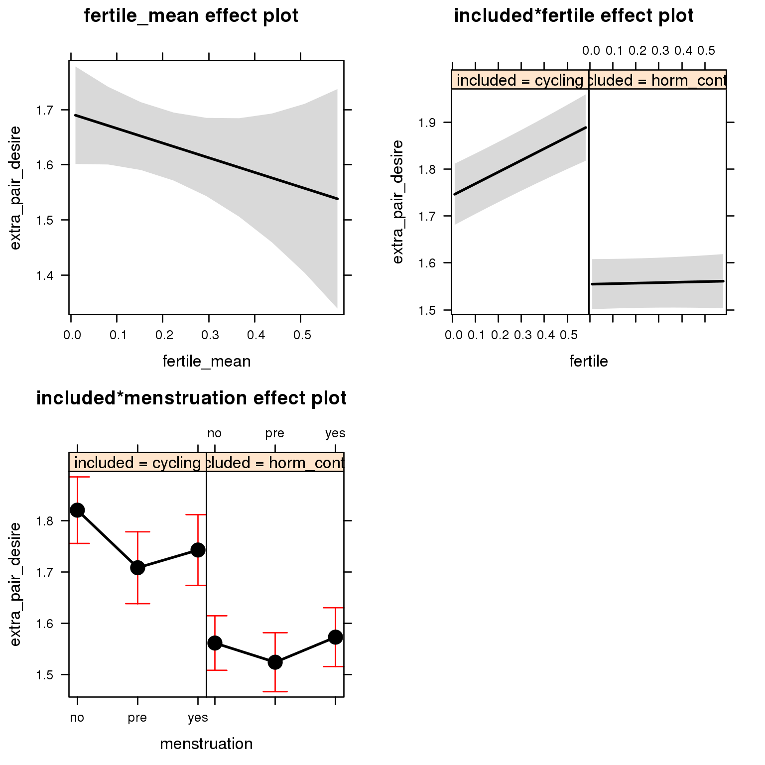
lmer(extra_pair_desire ~ included * (fertile + menstruation) + fertile_mean + in_pair_desire + (1 | person), data = diary) %->%
  m_extra_adjusted_for_in %>%
  print_summary()  %>%
  plot_all_effects()
##
##
## ```
## Linear mixed model fit by REML
## t-tests use Satterthwaite approximations to degrees of freedom ['lmerMod']
## Formula: extra_pair_desire ~ included * (fertile + menstruation) + fertile_mean +
## in_pair_desire + (1 | person)
## Data: diary
##
## REML criterion at convergence: 52299
##
## Scaled residuals:
## Min 1Q Median 3Q Max
## -4.814 -0.497 -0.133 0.338 7.392
##
## Random effects:
## Groups Name Variance Std.Dev.
## person (Intercept) 0.411 0.641
## Residual 0.367 0.606
## Number of obs: 26680, groups: person, 1054
##
## Fixed effects:
## Estimate Std. Error df t value Pr(>|t|)
## (Intercept) 1.94705 0.05461 1390.00000 35.66 < 2e-16 ***
## includedhorm_contra -0.20752 0.04382 1214.00000 -4.74 2.4e-06 ***
## fertile 0.25859 0.03737 25855.00000 6.92 4.6e-12 ***
## menstruationpre -0.11498 0.01851 25857.00000 -6.21 5.4e-10 ***
## menstruationyes -0.08455 0.01747 25949.00000 -4.84 1.3e-06 ***
## fertile_mean -0.26463 0.24239 1367.00000 -1.09 0.2751
## in_pair_desire -0.03564 0.00343 26489.00000 -10.39 < 2e-16 ***
## includedhorm_contra:fertile -0.25512 0.04739 25954.00000 -5.38 7.4e-08 ***
## includedhorm_contra:menstruationpre 0.07499 0.02377 25852.00000 3.16 0.0016 **
## includedhorm_contra:menstruationyes 0.09070 0.02288 25928.00000 3.96 7.4e-05 ***
## ---
## Signif. codes: 0 '***' 0.001 '**' 0.01 '*' 0.05 '.' 0.1 ' ' 1
##
## Correlation of Fixed Effects:
## (Intr) incld_ fertil mnstrtnp mnstrtny frtl_m in_pr_ inclddhrm_cntr:f
## inclddhrm_c -0.458
## fertile -0.119 0.209
## menstrutnpr -0.132 0.168 0.467
## menstrutnys -0.134 0.162 0.384 0.398
## fertile_men -0.753 -0.023 -0.056 -0.008 -0.005
## in_pair_dsr -0.218 -0.023 -0.024 0.013 0.037 0.000
## inclddhrm_cntr:f 0.117 -0.264 -0.787 -0.368 -0.302 0.009 0.034
## inclddhrm_cntr:mnstrtnp 0.107 -0.210 -0.363 -0.779 -0.310 -0.002 0.000 0.467
## inclddhrm_cntr:mnstrtny 0.102 -0.200 -0.293 -0.304 -0.763 -0.002 -0.006 0.381
## inclddhrm_cntr:mnstrtnp
## inclddhrm_c
## fertile
## menstrutnpr
## menstrutnys
## fertile_men
## in_pair_dsr
## inclddhrm_cntr:f
## inclddhrm_cntr:mnstrtnp
## inclddhrm_cntr:mnstrtny 0.384
##
## ```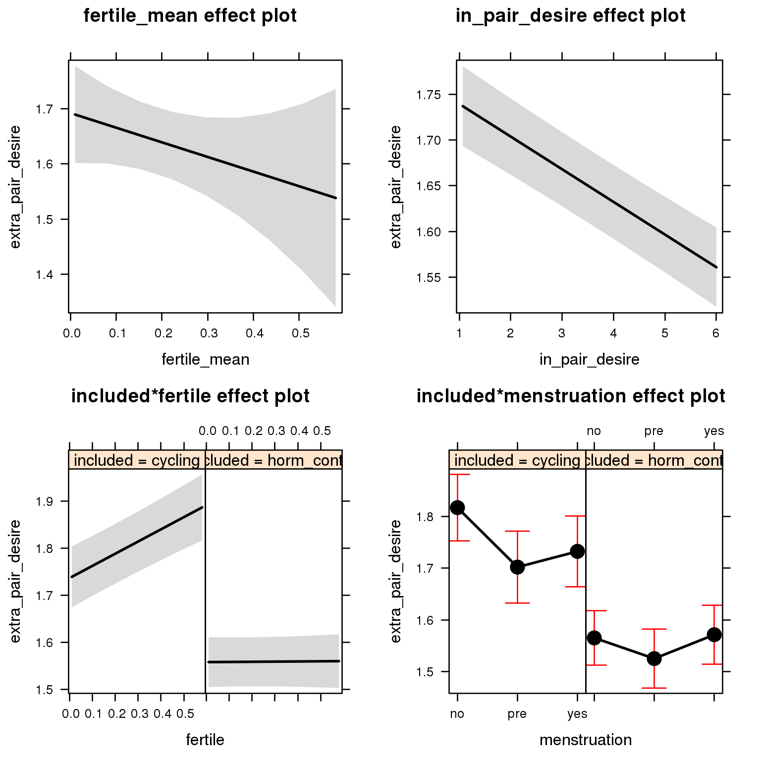
lmer(extra_pair_desire ~ included * (fertile + menstruation) + fertile_mean + scale(in_pair_desire) * included * fertile + fertile_mean + menstruation + (1 | person), data = diary) %->%
  m_extra_mod_by_in %>%
  print_summary()  %>%
  plot_triptych(x.var = "fertile", xlevels = 2)
##
##
## ```
## Linear mixed model fit by REML
## t-tests use Satterthwaite approximations to degrees of freedom ['lmerMod']
## Formula: extra_pair_desire ~ included * (fertile + menstruation) + fertile_mean +
## scale(in_pair_desire) * included * fertile + fertile_mean + menstruation + (1 | person)
## Data: diary
##
## REML criterion at convergence: 52316
##
## Scaled residuals:
## Min 1Q Median 3Q Max
## -4.812 -0.498 -0.133 0.337 7.394
##
## Random effects:
## Groups Name Variance Std.Dev.
## person (Intercept) 0.411 0.641
## Residual 0.367 0.606
## Number of obs: 26680, groups: person, 1054
##
## Fixed effects:
## Estimate Std. Error df t value Pr(>|t|)
## (Intercept) 1.81837 0.05330 1265.00000 34.12 < 2e-16 ***
## includedhorm_contra -0.20746 0.04382 1214.00000 -4.73 2.5e-06 ***
## fertile 0.25893 0.03739 25852.00000 6.92 4.5e-12 ***
## menstruationpre -0.11508 0.01852 25855.00000 -6.21 5.2e-10 ***
## menstruationyes -0.08472 0.01749 25949.00000 -4.84 1.3e-06 ***
## fertile_mean -0.26398 0.24239 1367.00000 -1.09 0.2763
## scale(in_pair_desire) -0.05222 0.00931 26432.00000 -5.61 2.0e-08 ***
## includedhorm_contra:fertile -0.25511 0.04742 25950.00000 -5.38 7.5e-08 ***
## includedhorm_contra:menstruationpre 0.07508 0.02377 25851.00000 3.16 0.0016 **
## includedhorm_contra:menstruationyes 0.09089 0.02292 25929.00000 3.97 7.3e-05 ***
## includedhorm_contra:scale(in_pair_desire) 0.00388 0.01199 26363.00000 0.32 0.7460
## fertile:scale(in_pair_desire) 0.01731 0.03135 25910.00000 0.55 0.5809
## includedhorm_contra:fertile:scale(in_pair_desire) -0.02389 0.04039 25861.00000 -0.59 0.5542
## ---
## Signif. codes: 0 '***' 0.001 '**' 0.01 '*' 0.05 '.' 0.1 ' ' 1
##
## ```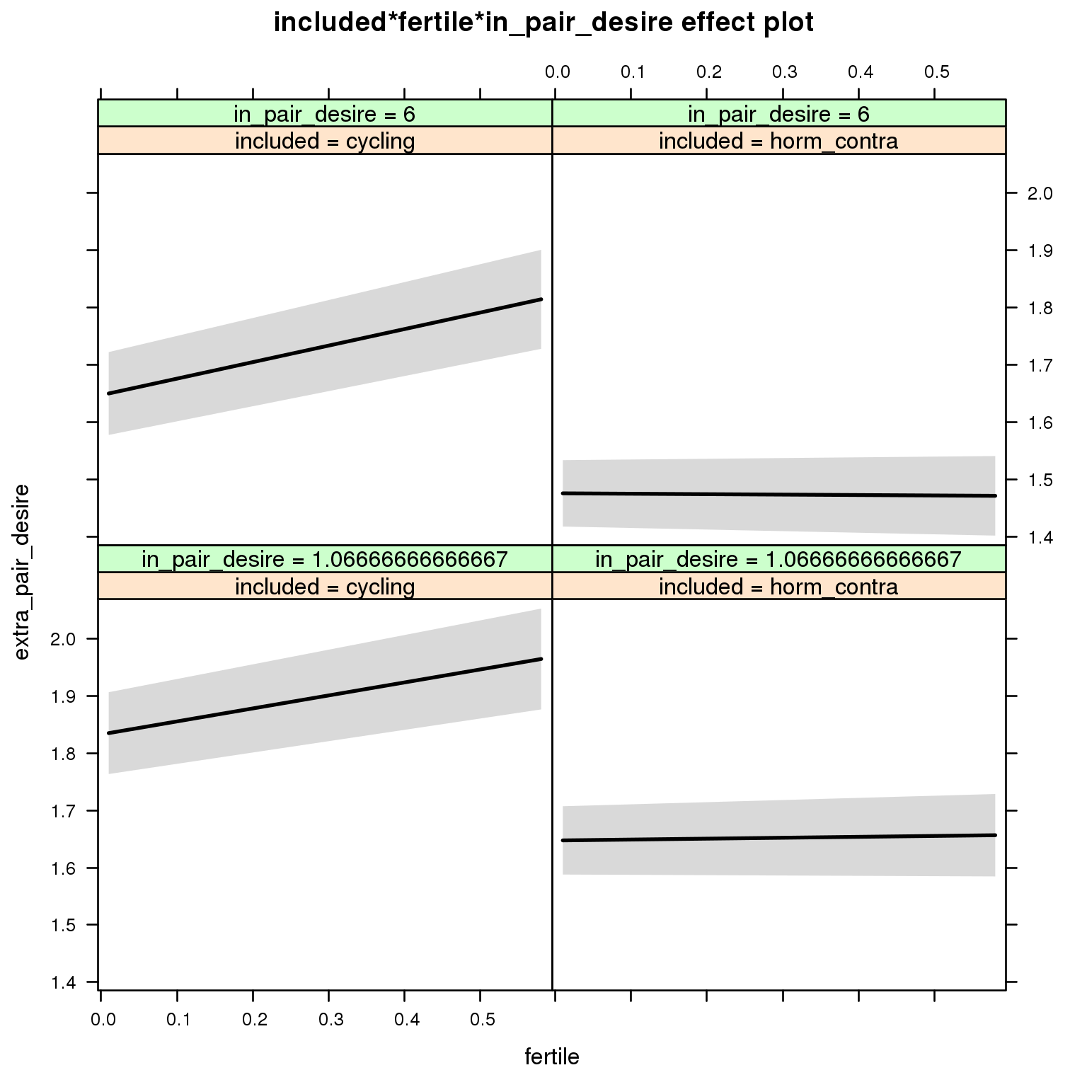
anova(m_extra_adjusted_for_in, m_extra_mod_by_in)## Data: diary
## Models:
## object: extra_pair_desire ~ included * (fertile + menstruation) + fertile_mean +
## object: in_pair_desire + (1 | person)
## ..1: extra_pair_desire ~ included * (fertile + menstruation) + fertile_mean +
## ..1: scale(in_pair_desire) * included * fertile + fertile_mean +
## ..1: menstruation + (1 | person)
## Df AIC BIC logLik deviance Chisq Chi Df Pr(>Chisq)
## object 12 52266 52364 -26121 52242
## ..1 15 52272 52394 -26121 52242 0.37 3 0.95lmer(in_pair_desire ~ included * (fertile + menstruation) + fertile_mean + scale(extra_pair_desire) * included * fertile + fertile_mean + menstruation + (1 | person), data = diary) %->%
m_in_mod_by_extra %>%
print_summary() %>%
plot_triptych(x.var = "fertile", xlevels = 2)##
##
## ```
## Linear mixed model fit by REML
## t-tests use Satterthwaite approximations to degrees of freedom ['lmerMod']
## Formula: in_pair_desire ~ included * (fertile + menstruation) + fertile_mean +
## scale(extra_pair_desire) * included * fertile + fertile_mean + menstruation + (1 | person)
## Data: diary
##
## REML criterion at convergence: 82972
##
## Scaled residuals:
## Min 1Q Median 3Q Max
## -3.529 -0.677 -0.028 0.665 3.745
##
## Random effects:
## Groups Name Variance Std.Dev.
## person (Intercept) 0.708 0.841
## Residual 1.184 1.088
## Number of obs: 26680, groups: person, 1054
##
## Fixed effects:
## Estimate Std. Error df t value Pr(>|t|)
## (Intercept) 3.49788 0.07453 1411.00000 46.93 < 2e-16 ***
## includedhorm_contra 0.26341 0.06100 1380.00000 4.32 1.7e-05 ***
## fertile 0.25194 0.06788 25984.00000 3.71 0.00021 ***
## menstruationpre -0.08354 0.03328 26005.00000 -2.51 0.01207 *
## menstruationyes -0.19894 0.03132 26117.00000 -6.35 2.2e-10 ***
## fertile_mean -0.00156 0.34203 1524.00000 0.00 0.99636
## scale(extra_pair_desire) -0.11931 0.01666 26318.00000 -7.16 8.2e-13 ***
## includedhorm_contra:fertile -0.45944 0.08566 26117.00000 -5.36 8.2e-08 ***
## includedhorm_contra:menstruationpre 0.00794 0.04269 26002.00000 0.19 0.85253
## includedhorm_contra:menstruationyes 0.05078 0.04104 26093.00000 1.24 0.21600
## includedhorm_contra:scale(extra_pair_desire) -0.00645 0.02289 26509.00000 -0.28 0.77823
## fertile:scale(extra_pair_desire) 0.16934 0.05052 26146.00000 3.35 0.00080 ***
## includedhorm_contra:fertile:scale(extra_pair_desire) -0.13265 0.07095 26059.00000 -1.87 0.06155 .
## ---
## Signif. codes: 0 '***' 0.001 '**' 0.01 '*' 0.05 '.' 0.1 ' ' 1
##
## ```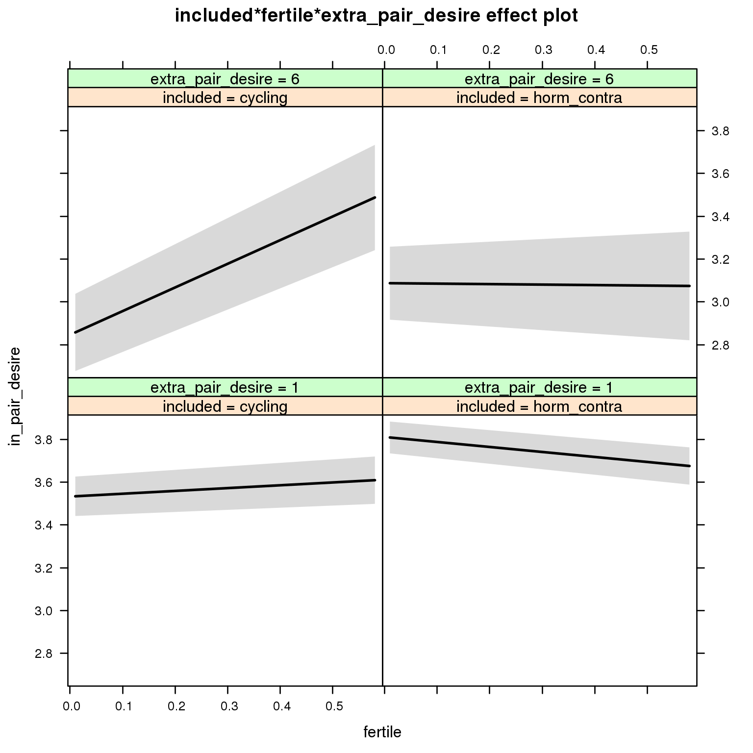
lmer(in_pair_desire ~ included * (fertile + menstruation) + fertile_mean + menstruation + (1 | person), data = diary) %->%
  m_in_not_adjusted_for_extra  %>%
  print_summary()  %>%
  plot_all_effects()
##
##
## ```
## Linear mixed model fit by REML
## t-tests use Satterthwaite approximations to degrees of freedom ['lmerMod']
## Formula: in_pair_desire ~ included * (fertile + menstruation) + fertile_mean +
## menstruation + (1 | person)
## Data: diary
##
## REML criterion at convergence: 83086
##
## Scaled residuals:
## Min 1Q Median 3Q Max
## -3.481 -0.678 -0.031 0.667 3.799
##
## Random effects:
## Groups Name Variance Std.Dev.
## person (Intercept) 0.736 0.858
## Residual 1.189 1.090
## Number of obs: 26680, groups: person, 1054
##
## Fixed effects:
## Estimate Std. Error df t value Pr(>|t|)
## (Intercept) 3.47053 0.07560 1399.00000 45.91 < 2e-16 ***
## includedhorm_contra 0.29330 0.06188 1365.00000 4.74 0.0000023616 ***
## fertile 0.26125 0.06714 25981.00000 3.89 0.0001 ***
## menstruationpre -0.06767 0.03327 26000.00000 -2.03 0.0419 *
## menstruationyes -0.18759 0.03135 26112.00000 -5.98 0.0000000022 ***
## fertile_mean 0.03371 0.34713 1518.00000 0.10 0.9227
## includedhorm_contra:fertile -0.47357 0.08505 26113.00000 -5.57 0.0000000260 ***
## includedhorm_contra:menstruationpre -0.00281 0.04271 25996.00000 -0.07 0.9475
## includedhorm_contra:menstruationyes 0.03767 0.04109 26088.00000 0.92 0.3593
## ---
## Signif. codes: 0 '***' 0.001 '**' 0.01 '*' 0.05 '.' 0.1 ' ' 1
##
## Correlation of Fixed Effects:
## (Intr) incld_ fertil mnstrtnp mnstrtny frtl_m inclddhrm_cntr:f
## inclddhrm_c -0.473
## fertile -0.163 0.266
## menstrutnpr -0.170 0.215 0.467
## menstrutnys -0.165 0.207 0.384 0.397
## fertile_men -0.772 -0.026 -0.069 -0.008 -0.005
## inclddhrm_cntr:f 0.163 -0.336 -0.786 -0.368 -0.303 0.010
## inclddhrm_cntr:mnstrtnp 0.140 -0.269 -0.363 -0.779 -0.309 -0.004 0.466
## inclddhrm_cntr:mnstrtny 0.132 -0.254 -0.293 -0.303 -0.763 -0.004 0.381
## inclddhrm_cntr:mnstrtnp
## inclddhrm_c
## fertile
## menstrutnpr
## menstrutnys
## fertile_men
## inclddhrm_cntr:f
## inclddhrm_cntr:mnstrtnp
## inclddhrm_cntr:mnstrtny 0.383
##
## ```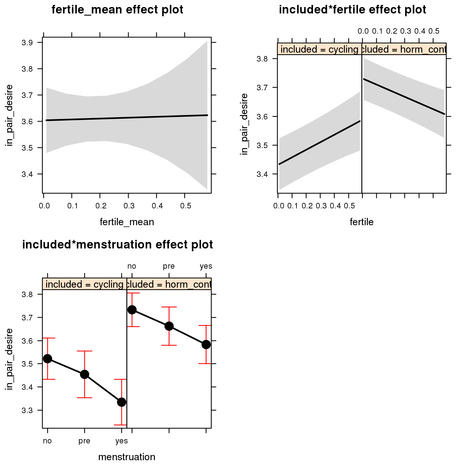
lmer(in_pair_desire ~ included * (fertile + menstruation) + fertile_mean + extra_pair_desire + (1 | person), data = diary) %->%
  m_in_adjusted_for_extra  %>%
  print_summary()  %>%
  plot_all_effects()
##
##
## ```
## Linear mixed model fit by REML
## t-tests use Satterthwaite approximations to degrees of freedom ['lmerMod']
## Formula: in_pair_desire ~ included * (fertile + menstruation) + fertile_mean +
## extra_pair_desire + (1 | person)
## Data: diary
##
## REML criterion at convergence: 82972
##
## Scaled residuals:
## Min 1Q Median 3Q Max
## -3.519 -0.678 -0.029 0.664 3.741
##
## Random effects:
## Groups Name Variance Std.Dev.
## person (Intercept) 0.708 0.841
## Residual 1.185 1.088
## Number of obs: 26680, groups: person, 1054
##
## Fixed effects:
## Estimate Std. Error df t value Pr(>|t|)
## (Intercept) 3.68760 0.07700 1584.00000 47.89 < 2e-16 ***
## includedhorm_contra 0.26761 0.06097 1377.00000 4.39 0.00001226486 ***
## fertile 0.29074 0.06708 25994.00000 4.33 0.00001466227 ***
## menstruationpre -0.08111 0.03323 26007.00000 -2.44 0.015 *
## menstruationyes -0.19680 0.03130 26121.00000 -6.29 0.00000000033 ***
## fertile_mean 0.00358 0.34207 1524.00000 0.01 0.992
## extra_pair_desire -0.11953 0.01082 26093.00000 -11.05 < 2e-16 ***
## includedhorm_contra:fertile -0.50139 0.08494 26126.00000 -5.90 0.00000000361 ***
## includedhorm_contra:menstruationpre 0.00631 0.04265 26003.00000 0.15 0.882
## includedhorm_contra:menstruationyes 0.04840 0.04103 26097.00000 1.18 0.238
## ---
## Signif. codes: 0 '***' 0.001 '**' 0.01 '*' 0.05 '.' 0.1 ' ' 1
##
## Correlation of Fixed Effects:
## (Intr) incld_ fertil mnstrtnp mnstrtny frtl_m extr__ inclddhrm_cntr:f
## inclddhrm_c -0.467
## fertile -0.149 0.267
## menstrutnpr -0.176 0.219 0.464
## menstrutnys -0.169 0.211 0.383 0.397
## fertile_men -0.749 -0.026 -0.070 -0.008 -0.005
## extr_pr_dsr -0.255 0.038 -0.040 0.037 0.027 0.008
## inclddhrm_cntr:f 0.152 -0.339 -0.787 -0.367 -0.302 0.010 0.030
## inclddhrm_cntr:mnstrtnp 0.142 -0.273 -0.362 -0.779 -0.309 -0.004 -0.020 0.465
## inclddhrm_cntr:mnstrtny 0.136 -0.258 -0.291 -0.303 -0.763 -0.004 -0.024 0.380
## inclddhrm_cntr:mnstrtnp
## inclddhrm_c
## fertile
## menstrutnpr
## menstrutnys
## fertile_men
## extr_pr_dsr
## inclddhrm_cntr:f
## inclddhrm_cntr:mnstrtnp
## inclddhrm_cntr:mnstrtny 0.383
##
## ```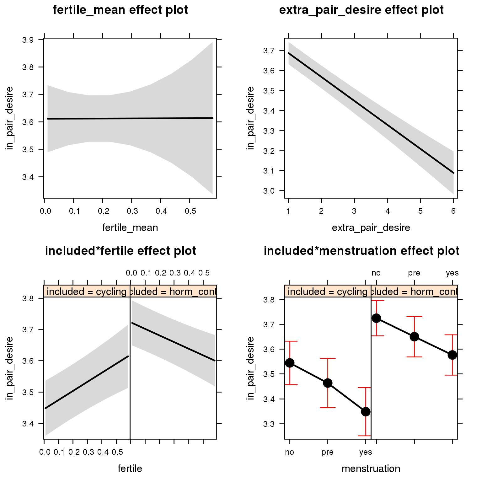
anova(m_in_adjusted_for_extra, m_in_mod_by_extra)## Data: diary
## Models:
## object: in_pair_desire ~ included * (fertile + menstruation) + fertile_mean +
## object: extra_pair_desire + (1 | person)
## ..1: in_pair_desire ~ included * (fertile + menstruation) + fertile_mean +
## ..1: scale(extra_pair_desire) * included * fertile + fertile_mean +
## ..1: menstruation + (1 | person)
## Df AIC BIC logLik deviance Chisq Chi Df Pr(>Chisq)
## object 12 82950 83048 -41463 82926
## ..1 15 82941 83064 -41456 82911 14.7 3 0.0021 **
## ---
## Signif. codes: 0 '***' 0.001 '**' 0.01 '*' 0.05 '.' 0.1 ' ' 1coefficients = bind_cols(bind_rows(
extra_not_adjusted_for_in = broom::tidy(m_extra_not_adjusted_for_in, conf.int = T),
extra_adjusted_for_in = broom::tidy(m_extra_adjusted_for_in, conf.int = T),
in_not_adjusted_for_extra = broom::tidy(m_in_not_adjusted_for_extra, conf.int = T),
in_adjusted_for_extra = broom::tidy(m_in_adjusted_for_extra, conf.int = T),
.id = c("model")
), bind_rows( broom::tidy(m_extra_not_adjusted_for_in, conf.int = T, level = 0.8),
broom::tidy(m_extra_adjusted_for_in, conf.int = T, level = 0.8),
broom::tidy(m_in_not_adjusted_for_extra, conf.int = T, level = 0.8),
broom::tidy(m_in_adjusted_for_extra, conf.int = T, level = 0.8)
) %>% select(conf.low, conf.high) %>% rename(conf.low80 = conf.low, conf.high80 = conf.high)
)Summary
coefficients  %>%
  filter(term %ends_with% "fertile") %>%
  ggplot(aes(x = model, y = estimate, ymin = conf.low, ymax = conf.high, color = term)) +
  geom_linerange(size = 0.5) +
  geom_pointrange(aes(ymin = conf.low80, ymax = conf.high80), size = 1) +
  scale_color_manual("Contraception status", values = c("includedhorm_contra:fertile"="black","fertile" = "red"), labels = c("includedhorm_contra:fertile"="hormonally\ncontracepting","fertile" = "fertile"), guide = F) +
  geom_hline(yintercept = 0, linetype = "dashed") +
  coord_flip()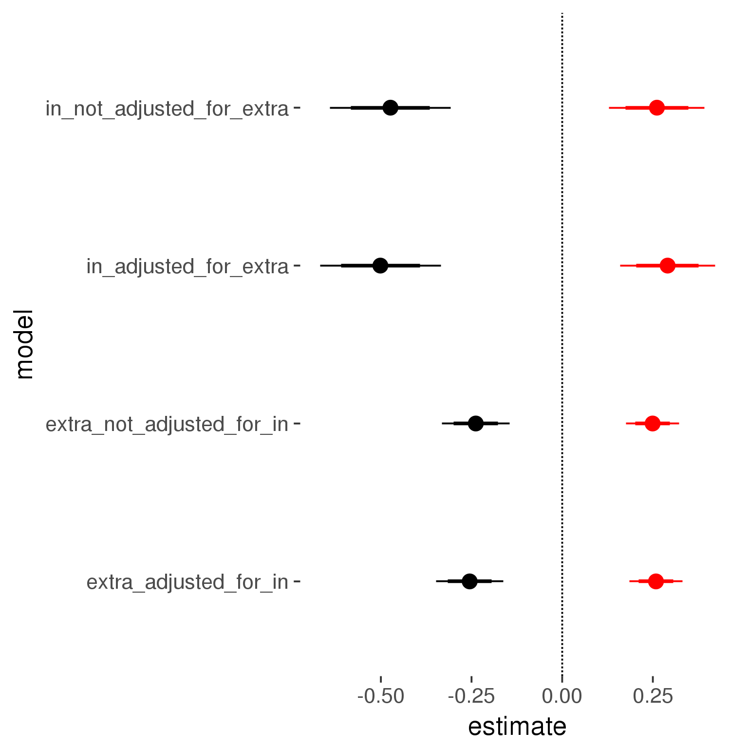
Awareness vs. regularity?
Are there stronger effects on extra pair desire in women using fertility-awareness-based contraception only because they have more regular cycles and so our fertility predictor is more useful?
No, it actually seems to be the other way around, cycle length no longer moderates the fertility effect when awareness is also included as a moderator.
lmer(extra_pair ~ contraceptive_methods * fertile + fertile_mean + menstruation + (1 | person), data = diary, subset = !is.na(included_lax) & contraceptive_method != "other") %->%
  m_extra_not_adjusted_for_length  %>%
  print_summary()  %>%
  plot_triptych(xlevels = 4, panel_rows = 1)
##
##
## ```
## Linear mixed model fit by REML
## t-tests use Satterthwaite approximations to degrees of freedom ['lmerMod']
## Formula: extra_pair ~ contraceptive_methods * fertile + fertile_mean + menstruation + (1 | person)
## Data: diary
## Subset: !is.na(included_lax) & contraceptive_method != "other"
##
## REML criterion at convergence: 30402
##
## Scaled residuals:
## Min 1Q Median 3Q Max
## -4.333 -0.557 -0.147 0.406 8.083
##
## Random effects:
## Groups Name Variance Std.Dev.
## person (Intercept) 0.320 0.566
## Residual 0.313 0.560
## Number of obs: 17026, groups: person, 513
##
## Fixed effects:
## Estimate Std. Error df t value Pr(>|t|)
## (Intercept) 1.87936 0.10617 518.00000 17.70 <2e-16 ***
## contraceptive_methodsfertility_awareness -0.07506 0.13288 524.00000 -0.56 0.572
## contraceptive_methodsnone -0.17512 0.14088 530.00000 -1.24 0.214
## contraceptive_methodshormonal -0.13113 0.06727 525.00000 -1.95 0.052 .
## fertile 0.11889 0.05531 16564.00000 2.15 0.032 *
## fertile_mean -0.11221 0.52225 519.00000 -0.21 0.830
## menstruationpre -0.03094 0.01323 16563.00000 -2.34 0.019 *
## menstruationyes 0.00506 0.01325 16569.00000 0.38 0.702
## contraceptive_methodsfertility_awareness:fertile 0.19271 0.11667 16569.00000 1.65 0.099 .
## contraceptive_methodsnone:fertile -0.01023 0.12973 16551.00000 -0.08 0.937
## contraceptive_methodshormonal:fertile -0.14470 0.05944 16575.00000 -2.43 0.015 *
## ---
## Signif. codes: 0 '***' 0.001 '**' 0.01 '*' 0.05 '.' 0.1 ' ' 1
##
## Correlation of Fixed Effects:
## (Intr) cntr__ cntrcptv_mthdsn cntrcptv_mthdsh fertil frtl_m mnstrtnp mnstrtny cnt__:
## cntrcptv_m_ -0.245
## cntrcptv_mthdsn -0.279 0.191
## cntrcptv_mthdsh -0.439 0.403 0.375
## fertile -0.077 0.065 0.060 0.133
## fertile_men -0.823 -0.012 0.047 -0.078 -0.025
## menstrutnpr -0.053 -0.001 -0.002 0.006 0.238 -0.002
## menstrutnys -0.046 0.000 0.002 0.008 0.189 -0.005 0.386
## cntrcptv__: 0.036 -0.150 -0.029 -0.061 -0.438 0.002 0.009 0.018
## cntrcptv_mthdsn: 0.030 -0.028 -0.143 -0.055 -0.395 0.005 0.007 0.007 0.188
## cntrcptv_mthdsh: 0.069 -0.061 -0.057 -0.151 -0.867 0.008 -0.006 0.007 0.411
## cntrcptv_mthdsn:
## cntrcptv_m_
## cntrcptv_mthdsn
## cntrcptv_mthdsh
## fertile
## fertile_men
## menstrutnpr
## menstrutnys
## cntrcptv__:
## cntrcptv_mthdsn:
## cntrcptv_mthdsh: 0.370
##
## ```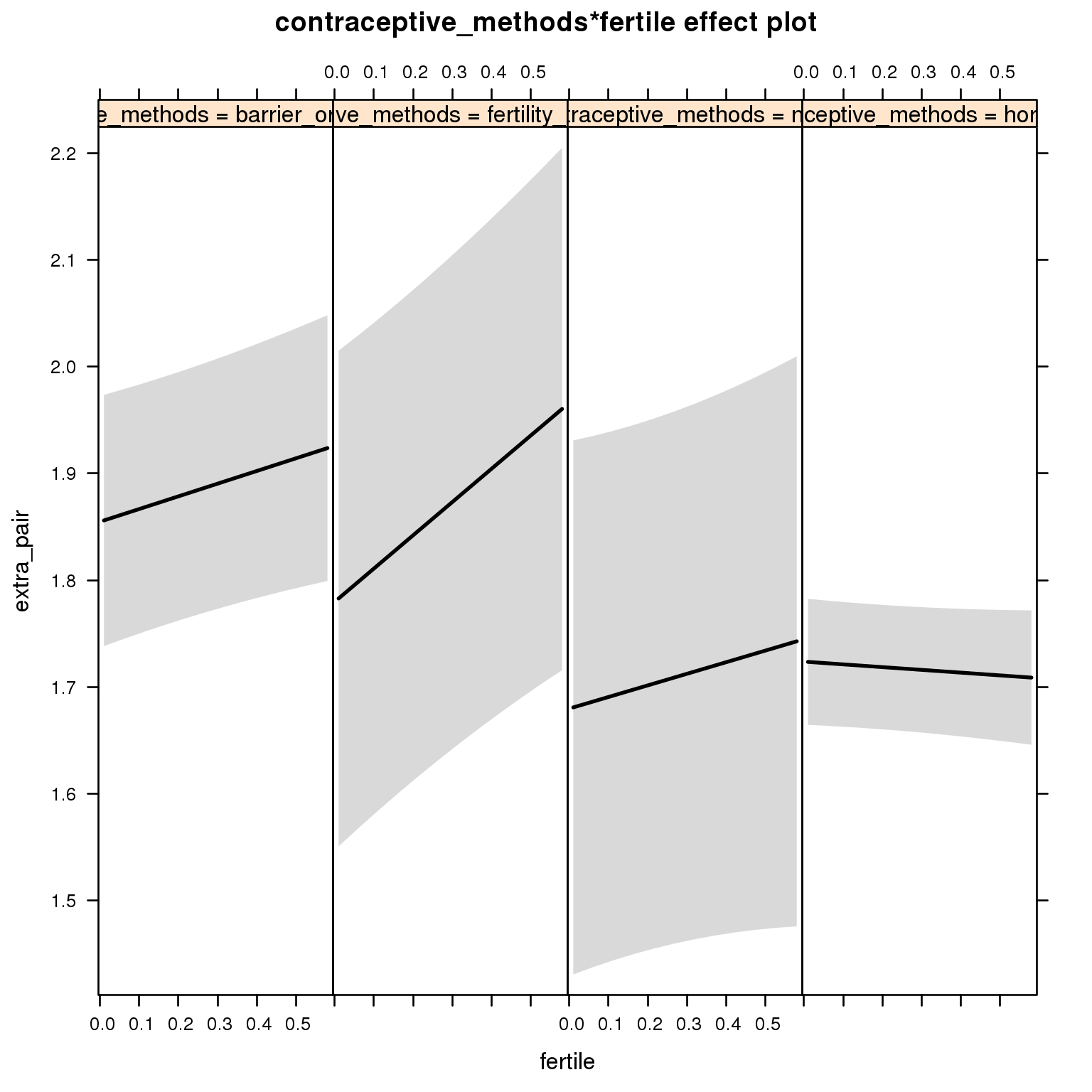
lmer(extra_pair ~ contraceptive_methods * fertile + cycle_length_groups * fertile + fertile_mean + menstruation + (1 | person), data = diary, subset = !is.na(included_lax) & contraceptive_method != "other") %>%
  calculate_effects() %->%
  m_extra_adjusted_for_length  %>%
  print_summary()  %>%
  plot_triptych(xlevels = 3, term = "fertile:cycle_length_groups", panel_rows = 1) %>%
  plot_triptych(xlevels = 4, term = "contraceptive_methods:fertile", panel_rows = 1)
##
##
## ```
## Linear mixed model fit by REML
## t-tests use Satterthwaite approximations to degrees of freedom ['lmerMod']
## Formula: extra_pair ~ contraceptive_methods * fertile + cycle_length_groups *
## fertile + fertile_mean + menstruation + (1 | person)
## Data: diary
## Subset: !is.na(included_lax) & contraceptive_method != "other"
##
## REML criterion at convergence: 30409
##
## Scaled residuals:
## Min 1Q Median 3Q Max
## -4.355 -0.556 -0.147 0.406 8.088
##
## Random effects:
## Groups Name Variance Std.Dev.
## person (Intercept) 0.321 0.566
## Residual 0.313 0.560
## Number of obs: 17026, groups: person, 513
##
## Fixed effects:
## Estimate Std. Error df t value Pr(>|t|)
## (Intercept) 1.88591 0.13059 520.00000 14.44 <2e-16 ***
## contraceptive_methodsfertility_awareness -0.07171 0.13312 522.00000 -0.54 0.5904
## contraceptive_methodsnone -0.17149 0.14124 528.00000 -1.21 0.2252
## contraceptive_methodshormonal -0.14096 0.06885 523.00000 -2.05 0.0411 *
## fertile 0.16004 0.08257 16549.00000 1.94 0.0526 .
## cycle_length_groups(25,30] 0.01582 0.07813 527.00000 0.20 0.8396
## cycle_length_groups(30,35] -0.05283 0.11587 525.00000 -0.46 0.6486
## fertile_mean -0.15500 0.52483 517.00000 -0.30 0.7679
## menstruationpre -0.03048 0.01323 16560.00000 -2.30 0.0212 *
## menstruationyes 0.00524 0.01326 16567.00000 0.40 0.6928
## contraceptive_methodsfertility_awareness:fertile 0.19965 0.11677 16566.00000 1.71 0.0873 .
## contraceptive_methodsnone:fertile 0.00858 0.13014 16550.00000 0.07 0.9474
## contraceptive_methodshormonal:fertile -0.17435 0.06104 16580.00000 -2.86 0.0043 **
## fertile:cycle_length_groups(25,30] -0.00525 0.06800 16539.00000 -0.08 0.9384
## fertile:cycle_length_groups(30,35] -0.18513 0.10377 16553.00000 -1.78 0.0744 .
## ---
## Signif. codes: 0 '***' 0.001 '**' 0.01 '*' 0.05 '.' 0.1 ' ' 1
##
## ```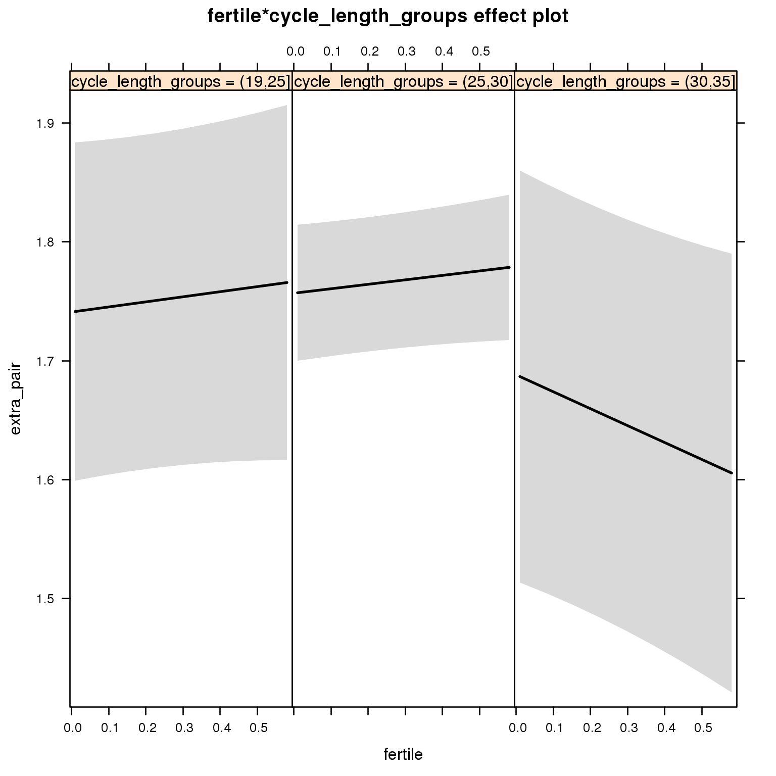

Extra-pair intimacy
model_summaries$extra_pair_intimacyModel summary
Model summary
model %>%
  print_summary()
Generalized linear mixed model fit by maximum likelihood (Laplace Approximation) ['glmerMod']
Family: binomial ( probit )
Formula: extra_pair_intimacy ~ included * (menstruation + fertile) + fertile_mean + (1 | person)
Data: diary
AIC BIC logLik deviance df.resid
2387 2469 -1184 2367 26693
Scaled residuals:
Min 1Q Median 3Q Max
-1.992 -0.003 -0.002 -0.002 7.512
Random effects:
Groups Name Variance Std.Dev.
person (Intercept) 7.36 2.71
Number of obs: 26703, groups: person, 1054
Fixed effects:
Estimate Std. Error z value Pr(>|z|)
(Intercept) -4.16420 0.26688 -15.60 <2e-16 ***
includedhorm_contra -0.10229 0.18833 -0.54 0.59
menstruationpre -0.03050 0.12101 -0.25 0.80
menstruationyes 0.00572 0.11425 0.05 0.96
fertile 0.23361 0.24845 0.94 0.35
fertile_mean -0.89089 1.32950 -0.67 0.50
includedhorm_contra:menstruationpre -0.13737 0.20691 -0.66 0.51
includedhorm_contra:menstruationyes -0.03488 0.19012 -0.18 0.85
includedhorm_contra:fertile -0.31393 0.39835 -0.79 0.43
---
Signif. codes: 0 '***' 0.001 '**' 0.01 '*' 0.05 '.' 0.1 ' ' 1
Correlation of Fixed Effects:
(Intr) incld_ mnstrtnp mnstrtny fertil frtl_m inclddhrm_cntr:mnstrtnp
inclddhrm_c -0.343
menstrutnpr -0.178 0.254
menstrutnys -0.174 0.242 0.367
fertile -0.175 0.340 0.449 0.347
fertile_men -0.805 -0.023 -0.003 0.004 -0.085
inclddhrm_cntr:mnstrtnp 0.119 -0.367 -0.585 -0.215 -0.261 -0.012
inclddhrm_cntr:mnstrtny 0.112 -0.358 -0.220 -0.601 -0.208 -0.009 0.340
inclddhrm_cntr:f 0.169 -0.505 -0.280 -0.217 -0.618 -0.019 0.436
inclddhrm_cntr:mnstrtny
inclddhrm_c
menstrutnpr
menstrutnys
fertile
fertile_men
inclddhrm_cntr:mnstrtnp
inclddhrm_cntr:mnstrtny
inclddhrm_cntr:f 0.342
convergence code: 0
Model failed to converge with max|grad| = 0.625484 (tol = 0.001, component 1)
Effect size standardised by residual variance (\(\frac{b}{ SD_{residual} }\)): 0.23 [-0.25;0.72].
Marginal effect plots
model %>%
  plot_all_effects()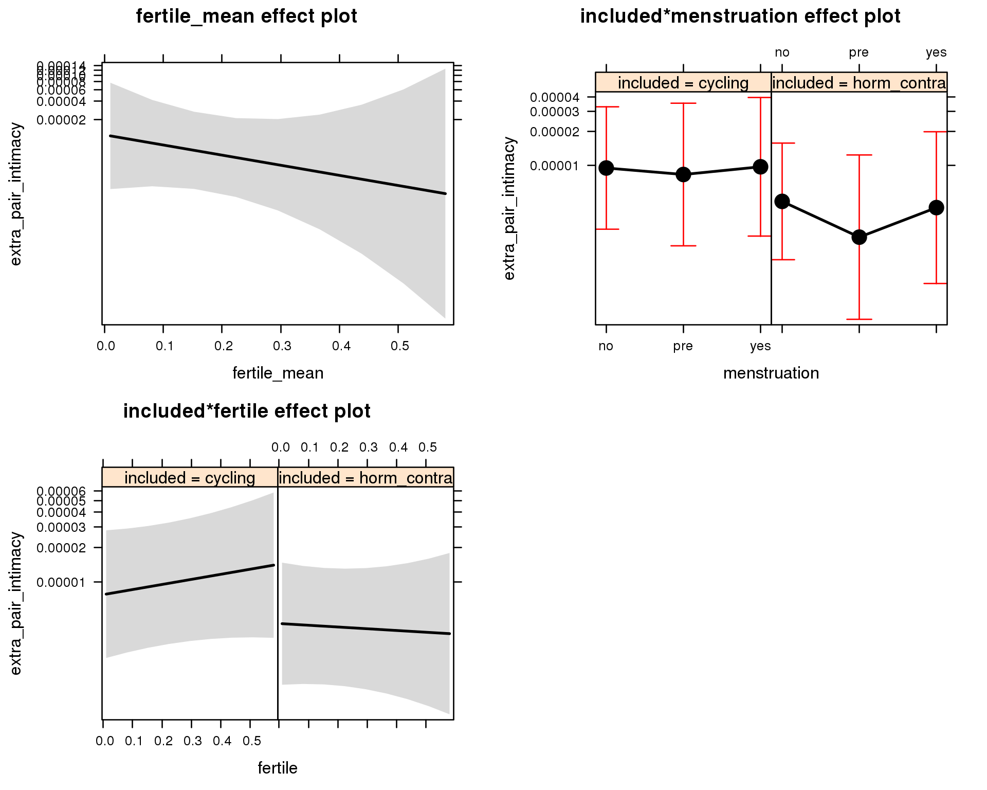
Outcome distribution
model %>%
  plot_outcome(diary) + xlab(outcome_label)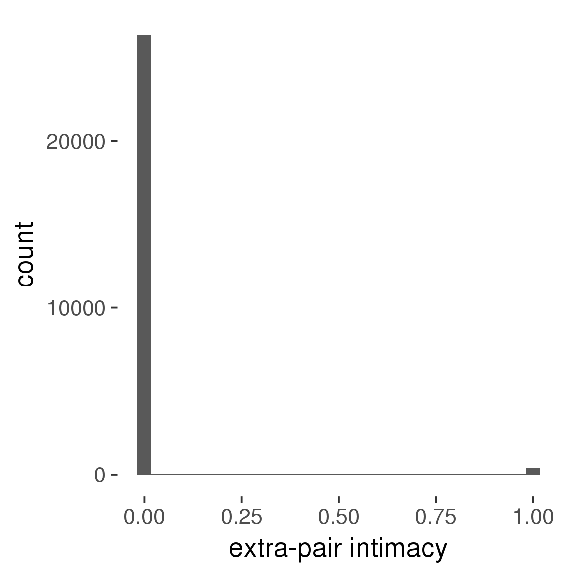
Diagnostics
model %>%
  print_diagnostics()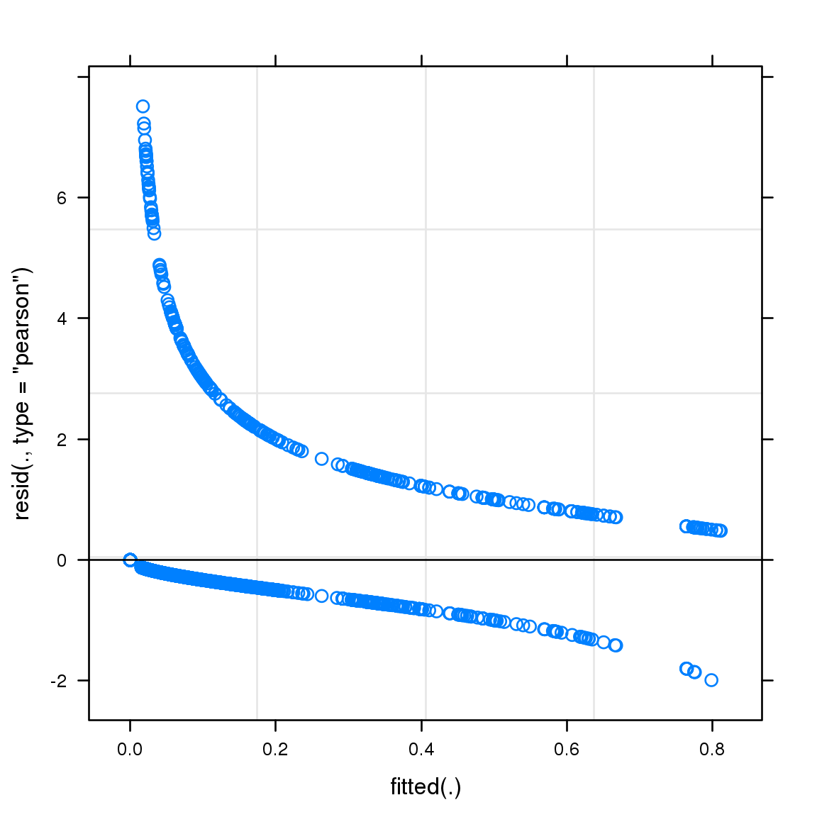

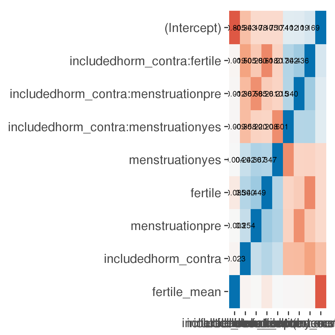
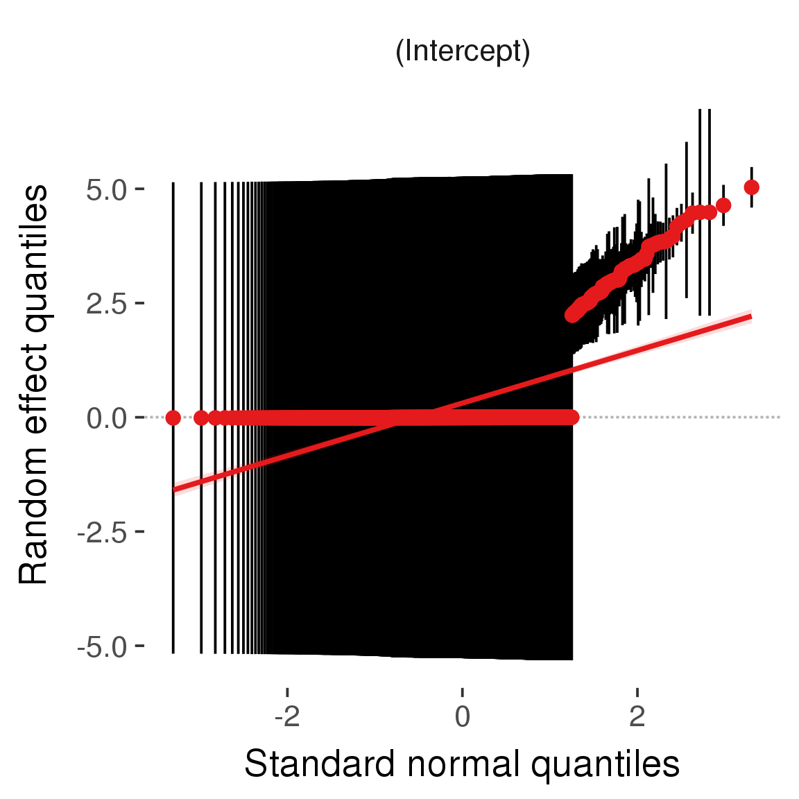
Curves
Here, we continuously plot the outcome over the course of the cycle. Because cycle lengths vary, we subset the data to cycles in a certain range. If the red curve traces the pink curve, our predictor accurately maps the relationship between fertile window probability and the outcome.
Cycle lengths from 21 to 36
Backward-counted
model %>%
  plot_curve(diary %>% filter(minimum_cycle_length_diary <= 36, minimum_cycle_length_diary > 20) %>% mutate(fertile=prc_stirn_b))
outcome = names(model@frame)[1]
outcome_label = recode(str_replace_all(str_replace_all(str_replace_all(outcome, "_", " "), " pair", "-pair"), " 1", ""),
"desirability 1" = "self-perceived desirability",
"NARQ admiration" = "narcissistic admiration",
"NARQ rivalry" = "narcissistic rivalry",
"extra-pair" = "extra-pair desire & behaviour",
"had sexual intercourse" = "sexual intercourse")
library(ggplot2)
# form a subset and run the model without the hormonal contraception and the fertility predictors
tmp = diary %>%
filter(!is.na(fertile), !is.na(included),
RCD > -1 * minimum_cycle_length_diary, RCD > -40)
new_form = update.formula(formula(model), new = . ~ . - fertile * included)
tmp$residuals = residuals(update(model, new_form, data = tmp , na.action = na.exclude))
tmp = tmp %>%
filter(!is.na(RCD), !is.na(residuals))
rcd_min = min(tmp$RCD)
tmp$real = FALSE
tmp_before = tmp
tmp_before$RCD = tmp_before$RCD + min(tmp$RCD) - 1
tmp_after = tmp
tmp_after$RCD = tmp_after$RCD - min(tmp$RCD) + 1
tmp$real = TRUE
tmp = bind_rows(tmp_before %>% filter(RCD > rcd_min - 11), tmp, tmp_after %>% filter(RCD < 11))GAM smooth on residuals
Here, we partialled out menstruation and individual random effects, then superimposed estimated probability of being in the fertile window scaled to the range of the estimated means. To address the periodicity of the cycle, we prepended and appended ten days of the timeseries to the end and the beginning of the timeseries. We then estimated the GAM and cut off the appended subsets before plotting.
tryCatch({
  trend_plot = ggplot(tmp,aes(x = RCD, y = residuals, colour = included)) +
    stat_smooth(geom = 'smooth',size = 0.8, fill = "#9ECAE1", method = 'gam', formula = y ~ s(x))
}, error = function(e){cat_message(e, "danger")})

tryCatch({
  trend_data = ggplot_build(trend_plot)$data[[1]]
}, error = function(e){cat_message(e, "danger")})

trend_data$RCD = round(trend_data$x)
trend_data = left_join(trend_data, tmp %>% select(real, RCD,fertile) %>% unique(), by = "RCD")
trend_data %>%
  filter(real == TRUE) %>%
  mutate(superimposed = ( ( (fertile - 0.01)/0.58) * (max(y)-min(y) ) ) + min(y) ) ->
  trend_data


ggplot(trend_data) +
  geom_ribbon(aes(x = x, ymin = ymin, ymax = ymax,  fill = factor(group)), alpha = 0.2) +
  geom_line(aes(x = x, y = y, colour = factor(group)), size = 0.8, stat = "identity") +
  scale_x_continuous(caption_x) +
  geom_line(aes(x = x, y = superimposed), color = "#a83fbf", size = 1, linetype = 'dashed') +
  annotate("text",x = mean(trend_data$x),  y = max(trend_data$superimposed,na.rm=T) + 0.1, label = 'superimposed fertility peak', color = "#a83fbf") +
  scale_y_continuous(outcome_label) +
  ggtitle("GAM smooth, residuals") +
  scale_color_manual("Contraception status",values = c("2"="black","1"= "red"), labels = c("2"="hormonally\ncontracepting","1"="cycling"), guide = F) +
  scale_fill_manual("Contraception status",values = c("2"="black","1"= "red"), labels = c("2"="hormonally\ncontracepting","1"="cycling"), guide = F)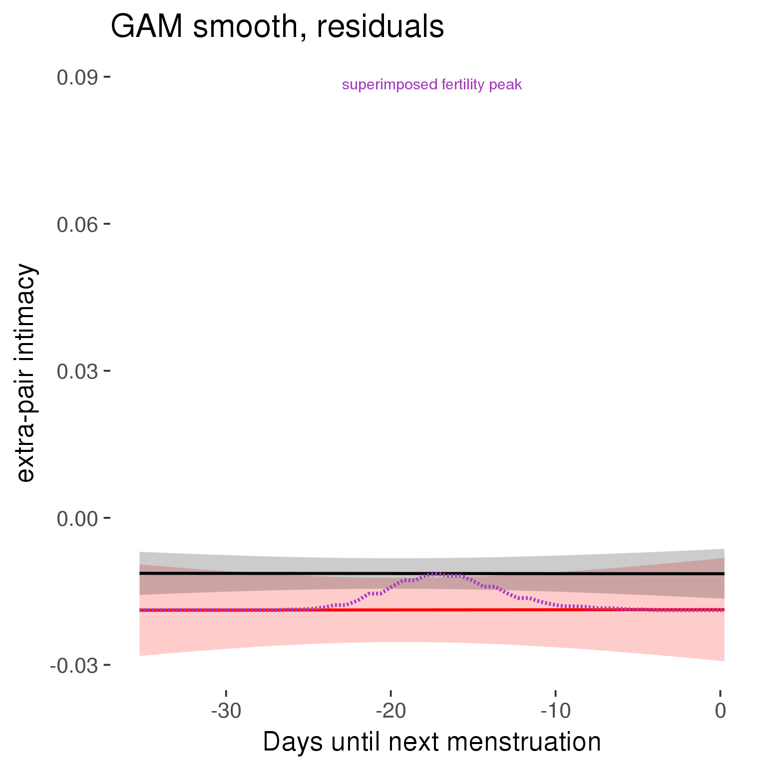
GAM smooth on raw data
As before, but without partialling anything out.
tryCatch({
  trend_plot = ggplot(tmp,aes_string(x = "RCD", y = outcome, colour = "included")) +
    stat_smooth(geom = 'smooth',size = 0.8, fill = "#9ECAE1", method = 'gam', formula = y ~ s(x))
}, error = function(e){cat_message(e, "danger")})

tryCatch({
  trend_data = ggplot_build(trend_plot)$data[[1]]
}, error = function(e){cat_message(e, "danger")})

trend_data$RCD = round(trend_data$x)
trend_data = left_join(trend_data, tmp %>% select(real, RCD,fertile) %>% unique(), by = "RCD")
trend_data %>%
  filter(real == TRUE) %>%
  mutate(superimposed = ( ( (fertile - 0.01)/0.58) * (max(y)-min(y) ) ) + min(y) ) ->
  trend_data

plot1b = ggplot(trend_data) +
  geom_ribbon(aes(x = x, ymin = ymin, ymax = ymax,  fill = factor(group)), alpha = 0.2) +
  geom_line(aes(x = x, y = y, colour = factor(group)), size = 0.8, stat = "identity") +
  scale_x_continuous(caption_x) +
  geom_line(aes(x = x, y = superimposed), color = "#a83fbf", size = 1, linetype = 'dashed') +
  annotate("text",x = mean(trend_data$x),  y = max(trend_data$superimposed,na.rm=T) + 0.1, label = 'superimposed fertility peak', color = "#a83fbf") +
  scale_y_continuous(outcome_label) +
  ggtitle("GAM smooth, raw data") +
  scale_color_manual("Contraception status",values = c("2"="black","1"= "red"), labels = c("2"="hormonally\ncontracepting","1"="cycling"), guide = F) +
  scale_fill_manual("Contraception status",values = c("2"="black","1"= "red"), labels = c("2"="hormonally\ncontracepting","1"="cycling"), guide = F)

suppressWarnings(print(plot1b))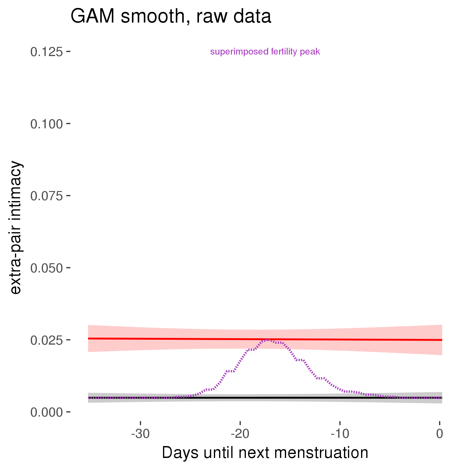
Means and standard errors over raw data
Nothing partialled out, just straight means with bootstrapped confidence intervals.
tryCatch({
  trend_plot = ggplot(tmp,aes_string(x = "RCD", y = outcome, colour = "included")) +
    geom_pointrange(size = 0.8, stat = 'summary', fun.data = "mean_cl_boot")
}, error = function(e){cat_message(e, "danger")})
tryCatch({
  trend_data = ggplot_build(trend_plot)$data[[1]]
}, error = function(e){cat_message(e, "danger")})

trend_data$RCD = round(trend_data$x)
trend_data = left_join(trend_data, tmp %>% select(real, RCD,fertile) %>% unique(), by = "RCD")
trend_data %>%
  filter(real == TRUE) %>%
  mutate(superimposed = ( ( (fertile - 0.01)/0.58) * (max(y)-min(y) ) ) + min(y) ) ->
  trend_data

plot3 = ggplot(trend_data) +
  geom_pointrange(aes(x = x, y = y, ymin = ymin,ymax = ymax, colour = factor(group)), size = 0.8, stat = "identity", alpha = 0.6, position = position_dodge(width = .5)) +
  scale_x_continuous("Days until next menstruation") +
  geom_line(aes(x= x, y = superimposed), color = "#a83fbf", size = 1, linetype = 'dashed') +
  annotate("text",x = mean(trend_data$x),  y = max(trend_data$superimposed,na.rm=T) + 0.1, label = 'superimposed fertility peak', color = "#a83fbf") +
  scale_y_continuous(outcome_label) +
  ggtitle("Means with standard errors, raw data") +
  scale_color_manual("Contraception status",values = c("2"="black","1"= "red"), labels = c("2"="hormonally\ncontracepting","1"="cycling"), guide = F) +
  scale_fill_manual("Contraception status",values = c("2"="black","1"= "red"), labels = c("2"="hormonally\ncontracepting","1"="cycling"), guide = F)
suppressWarnings(print(plot3))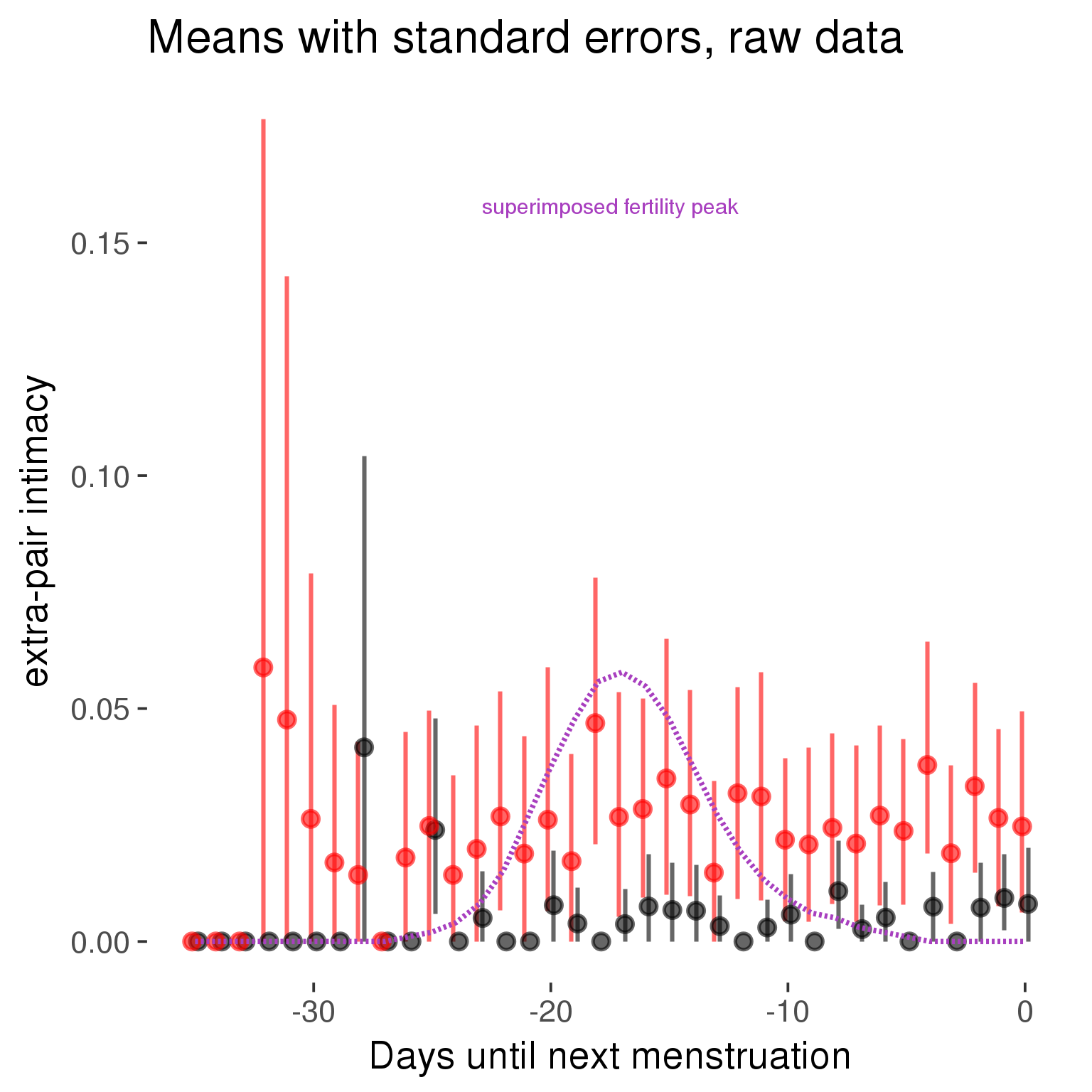
Forward-counted
model %>%
  plot_curve(diary %>% filter(minimum_cycle_length_diary <= 36, minimum_cycle_length_diary > 20) %>% mutate(RCD = FCD, fertile = prc_stirn_b_forward_counted), caption_x = "Days since last menstruation")
outcome = names(model@frame)[1]
outcome_label = recode(str_replace_all(str_replace_all(str_replace_all(outcome, "_", " "), " pair", "-pair"), " 1", ""),
"desirability 1" = "self-perceived desirability",
"NARQ admiration" = "narcissistic admiration",
"NARQ rivalry" = "narcissistic rivalry",
"extra-pair" = "extra-pair desire & behaviour",
"had sexual intercourse" = "sexual intercourse")
library(ggplot2)
# form a subset and run the model without the hormonal contraception and the fertility predictors
tmp = diary %>%
filter(!is.na(fertile), !is.na(included),
RCD > -1 * minimum_cycle_length_diary, RCD > -40)
new_form = update.formula(formula(model), new = . ~ . - fertile * included)
tmp$residuals = residuals(update(model, new_form, data = tmp , na.action = na.exclude))
tmp = tmp %>%
filter(!is.na(RCD), !is.na(residuals))
rcd_min = min(tmp$RCD)
tmp$real = FALSE
tmp_before = tmp
tmp_before$RCD = tmp_before$RCD + min(tmp$RCD) - 1
tmp_after = tmp
tmp_after$RCD = tmp_after$RCD - min(tmp$RCD) + 1
tmp$real = TRUE
tmp = bind_rows(tmp_before %>% filter(RCD > rcd_min - 11), tmp, tmp_after %>% filter(RCD < 11))GAM smooth on residuals
Here, we partialled out menstruation and individual random effects, then superimposed estimated probability of being in the fertile window scaled to the range of the estimated means. To address the periodicity of the cycle, we prepended and appended ten days of the timeseries to the end and the beginning of the timeseries. We then estimated the GAM and cut off the appended subsets before plotting.
tryCatch({
  trend_plot = ggplot(tmp,aes(x = RCD, y = residuals, colour = included)) +
    stat_smooth(geom = 'smooth',size = 0.8, fill = "#9ECAE1", method = 'gam', formula = y ~ s(x))
}, error = function(e){cat_message(e, "danger")})

tryCatch({
  trend_data = ggplot_build(trend_plot)$data[[1]]
}, error = function(e){cat_message(e, "danger")})

trend_data$RCD = round(trend_data$x)
trend_data = left_join(trend_data, tmp %>% select(real, RCD,fertile) %>% unique(), by = "RCD")
trend_data %>%
  filter(real == TRUE) %>%
  mutate(superimposed = ( ( (fertile - 0.01)/0.58) * (max(y)-min(y) ) ) + min(y) ) ->
  trend_data


ggplot(trend_data) +
  geom_ribbon(aes(x = x, ymin = ymin, ymax = ymax,  fill = factor(group)), alpha = 0.2) +
  geom_line(aes(x = x, y = y, colour = factor(group)), size = 0.8, stat = "identity") +
  scale_x_continuous(caption_x) +
  geom_line(aes(x = x, y = superimposed), color = "#a83fbf", size = 1, linetype = 'dashed') +
  annotate("text",x = mean(trend_data$x),  y = max(trend_data$superimposed,na.rm=T) + 0.1, label = 'superimposed fertility peak', color = "#a83fbf") +
  scale_y_continuous(outcome_label) +
  ggtitle("GAM smooth, residuals") +
  scale_color_manual("Contraception status",values = c("2"="black","1"= "red"), labels = c("2"="hormonally\ncontracepting","1"="cycling"), guide = F) +
  scale_fill_manual("Contraception status",values = c("2"="black","1"= "red"), labels = c("2"="hormonally\ncontracepting","1"="cycling"), guide = F)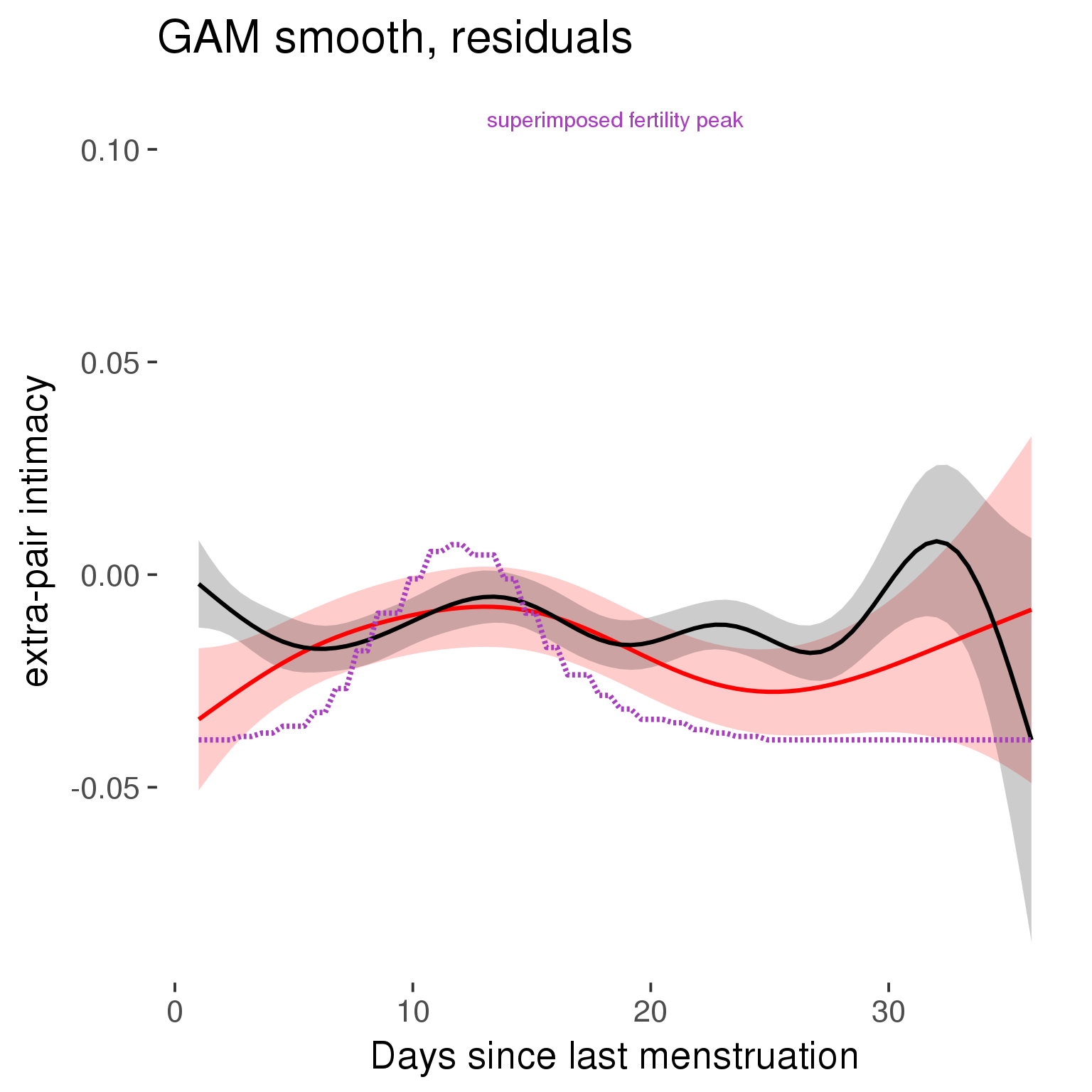
GAM smooth on raw data
As before, but without partialling anything out.
tryCatch({
  trend_plot = ggplot(tmp,aes_string(x = "RCD", y = outcome, colour = "included")) +
    stat_smooth(geom = 'smooth',size = 0.8, fill = "#9ECAE1", method = 'gam', formula = y ~ s(x))
}, error = function(e){cat_message(e, "danger")})

tryCatch({
  trend_data = ggplot_build(trend_plot)$data[[1]]
}, error = function(e){cat_message(e, "danger")})

trend_data$RCD = round(trend_data$x)
trend_data = left_join(trend_data, tmp %>% select(real, RCD,fertile) %>% unique(), by = "RCD")
trend_data %>%
  filter(real == TRUE) %>%
  mutate(superimposed = ( ( (fertile - 0.01)/0.58) * (max(y)-min(y) ) ) + min(y) ) ->
  trend_data

plot1b = ggplot(trend_data) +
  geom_ribbon(aes(x = x, ymin = ymin, ymax = ymax,  fill = factor(group)), alpha = 0.2) +
  geom_line(aes(x = x, y = y, colour = factor(group)), size = 0.8, stat = "identity") +
  scale_x_continuous(caption_x) +
  geom_line(aes(x = x, y = superimposed), color = "#a83fbf", size = 1, linetype = 'dashed') +
  annotate("text",x = mean(trend_data$x),  y = max(trend_data$superimposed,na.rm=T) + 0.1, label = 'superimposed fertility peak', color = "#a83fbf") +
  scale_y_continuous(outcome_label) +
  ggtitle("GAM smooth, raw data") +
  scale_color_manual("Contraception status",values = c("2"="black","1"= "red"), labels = c("2"="hormonally\ncontracepting","1"="cycling"), guide = F) +
  scale_fill_manual("Contraception status",values = c("2"="black","1"= "red"), labels = c("2"="hormonally\ncontracepting","1"="cycling"), guide = F)

suppressWarnings(print(plot1b))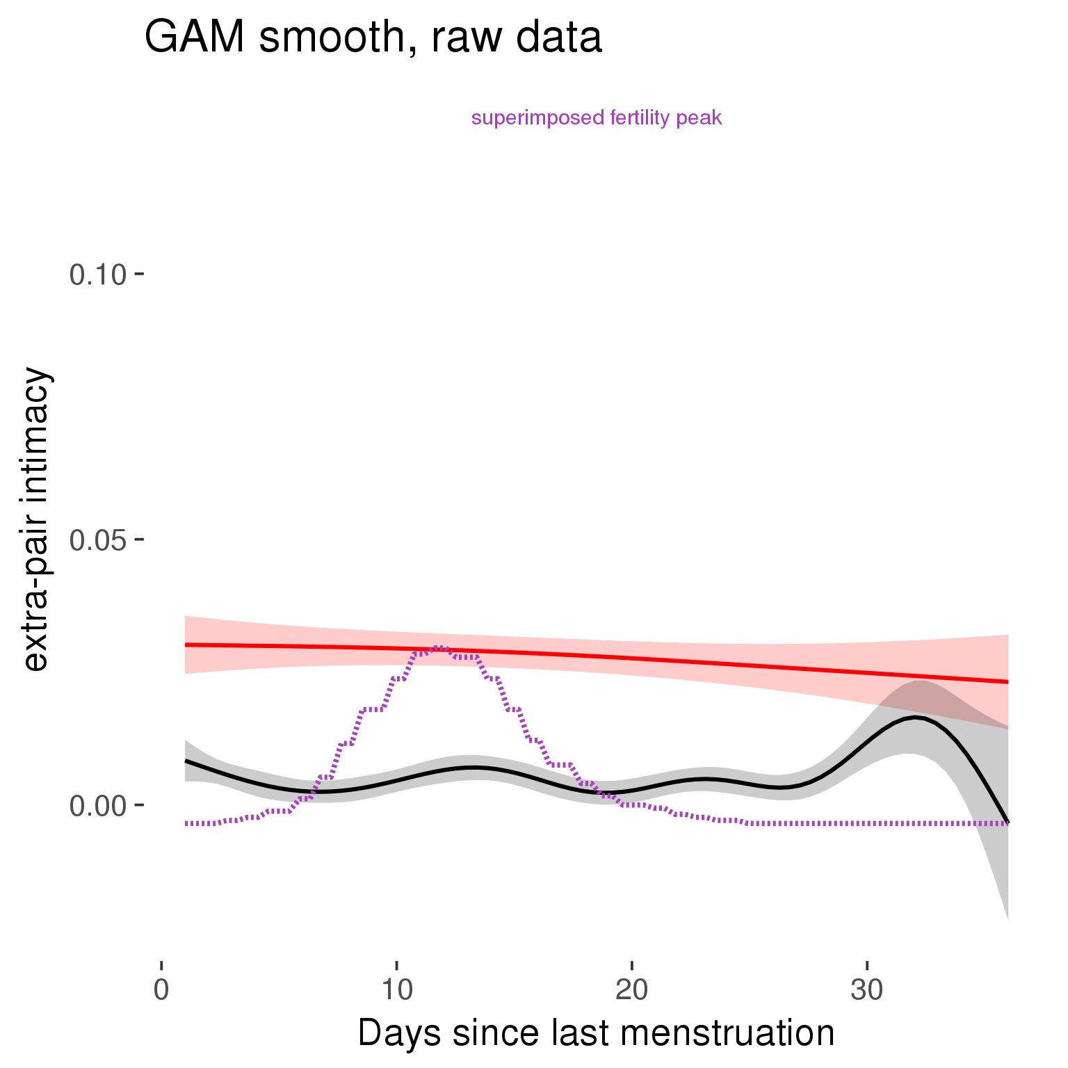
Means and standard errors over raw data
Nothing partialled out, just straight means with bootstrapped confidence intervals.
tryCatch({
  trend_plot = ggplot(tmp,aes_string(x = "RCD", y = outcome, colour = "included")) +
    geom_pointrange(size = 0.8, stat = 'summary', fun.data = "mean_cl_boot")
}, error = function(e){cat_message(e, "danger")})
tryCatch({
  trend_data = ggplot_build(trend_plot)$data[[1]]
}, error = function(e){cat_message(e, "danger")})

trend_data$RCD = round(trend_data$x)
trend_data = left_join(trend_data, tmp %>% select(real, RCD,fertile) %>% unique(), by = "RCD")
trend_data %>%
  filter(real == TRUE) %>%
  mutate(superimposed = ( ( (fertile - 0.01)/0.58) * (max(y)-min(y) ) ) + min(y) ) ->
  trend_data

plot3 = ggplot(trend_data) +
  geom_pointrange(aes(x = x, y = y, ymin = ymin,ymax = ymax, colour = factor(group)), size = 0.8, stat = "identity", alpha = 0.6, position = position_dodge(width = .5)) +
  scale_x_continuous("Days until next menstruation") +
  geom_line(aes(x= x, y = superimposed), color = "#a83fbf", size = 1, linetype = 'dashed') +
  annotate("text",x = mean(trend_data$x),  y = max(trend_data$superimposed,na.rm=T) + 0.1, label = 'superimposed fertility peak', color = "#a83fbf") +
  scale_y_continuous(outcome_label) +
  ggtitle("Means with standard errors, raw data") +
  scale_color_manual("Contraception status",values = c("2"="black","1"= "red"), labels = c("2"="hormonally\ncontracepting","1"="cycling"), guide = F) +
  scale_fill_manual("Contraception status",values = c("2"="black","1"= "red"), labels = c("2"="hormonally\ncontracepting","1"="cycling"), guide = F)
suppressWarnings(print(plot3))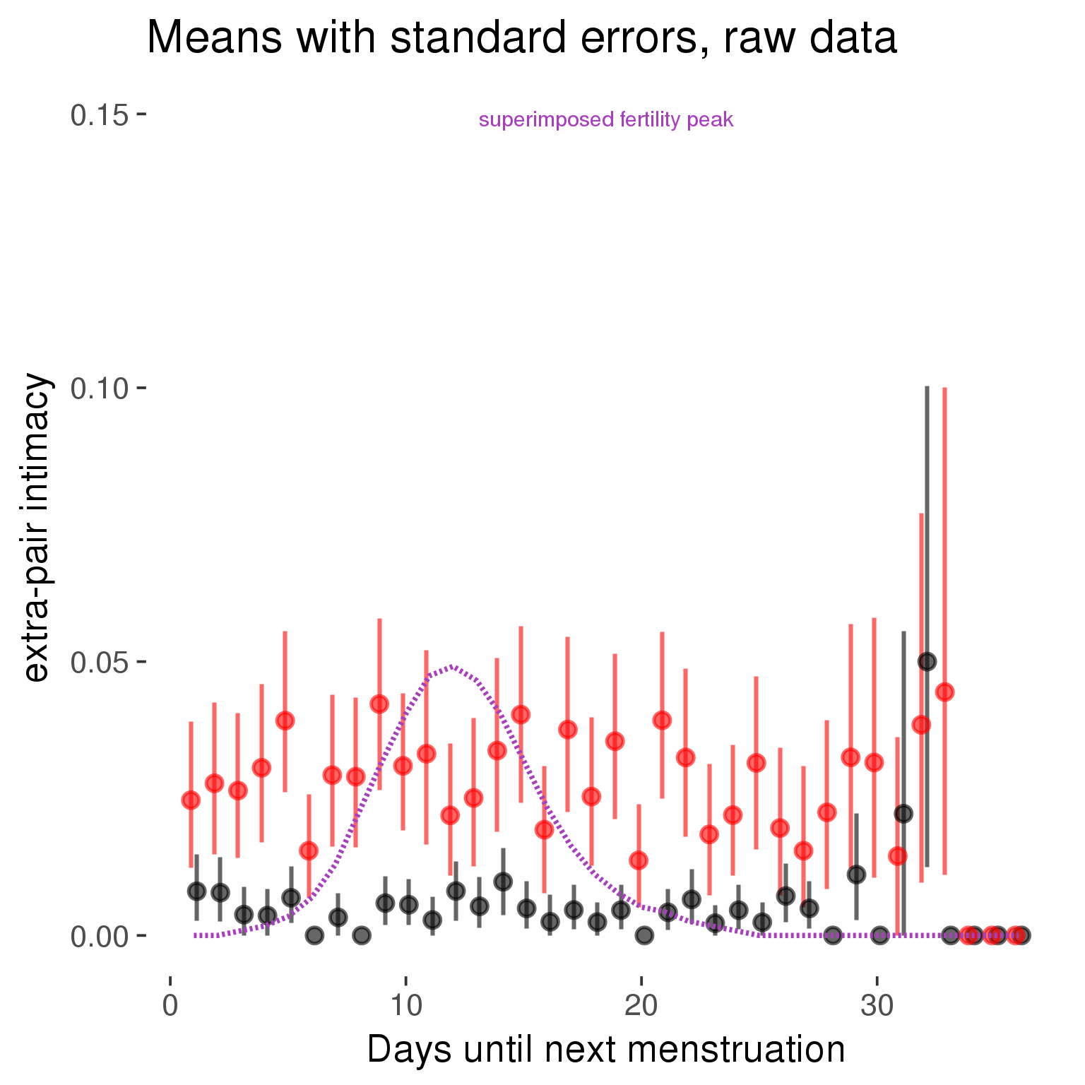
Cycle lengths from 27 to 30
Backward-counted
model %>%
  plot_curve(diary %>% filter(minimum_cycle_length_diary <= 30, minimum_cycle_length_diary >= 27) %>% mutate(fertile=prc_stirn_b))
outcome = names(model@frame)[1]
outcome_label = recode(str_replace_all(str_replace_all(str_replace_all(outcome, "_", " "), " pair", "-pair"), " 1", ""),
"desirability 1" = "self-perceived desirability",
"NARQ admiration" = "narcissistic admiration",
"NARQ rivalry" = "narcissistic rivalry",
"extra-pair" = "extra-pair desire & behaviour",
"had sexual intercourse" = "sexual intercourse")
library(ggplot2)
# form a subset and run the model without the hormonal contraception and the fertility predictors
tmp = diary %>%
filter(!is.na(fertile), !is.na(included),
RCD > -1 * minimum_cycle_length_diary, RCD > -40)
new_form = update.formula(formula(model), new = . ~ . - fertile * included)
tmp$residuals = residuals(update(model, new_form, data = tmp , na.action = na.exclude))
tmp = tmp %>%
filter(!is.na(RCD), !is.na(residuals))
rcd_min = min(tmp$RCD)
tmp$real = FALSE
tmp_before = tmp
tmp_before$RCD = tmp_before$RCD + min(tmp$RCD) - 1
tmp_after = tmp
tmp_after$RCD = tmp_after$RCD - min(tmp$RCD) + 1
tmp$real = TRUE
tmp = bind_rows(tmp_before %>% filter(RCD > rcd_min - 11), tmp, tmp_after %>% filter(RCD < 11))GAM smooth on residuals
Here, we partialled out menstruation and individual random effects, then superimposed estimated probability of being in the fertile window scaled to the range of the estimated means. To address the periodicity of the cycle, we prepended and appended ten days of the timeseries to the end and the beginning of the timeseries. We then estimated the GAM and cut off the appended subsets before plotting.
tryCatch({
  trend_plot = ggplot(tmp,aes(x = RCD, y = residuals, colour = included)) +
    stat_smooth(geom = 'smooth',size = 0.8, fill = "#9ECAE1", method = 'gam', formula = y ~ s(x))
}, error = function(e){cat_message(e, "danger")})

tryCatch({
  trend_data = ggplot_build(trend_plot)$data[[1]]
}, error = function(e){cat_message(e, "danger")})

trend_data$RCD = round(trend_data$x)
trend_data = left_join(trend_data, tmp %>% select(real, RCD,fertile) %>% unique(), by = "RCD")
trend_data %>%
  filter(real == TRUE) %>%
  mutate(superimposed = ( ( (fertile - 0.01)/0.58) * (max(y)-min(y) ) ) + min(y) ) ->
  trend_data


ggplot(trend_data) +
  geom_ribbon(aes(x = x, ymin = ymin, ymax = ymax,  fill = factor(group)), alpha = 0.2) +
  geom_line(aes(x = x, y = y, colour = factor(group)), size = 0.8, stat = "identity") +
  scale_x_continuous(caption_x) +
  geom_line(aes(x = x, y = superimposed), color = "#a83fbf", size = 1, linetype = 'dashed') +
  annotate("text",x = mean(trend_data$x),  y = max(trend_data$superimposed,na.rm=T) + 0.1, label = 'superimposed fertility peak', color = "#a83fbf") +
  scale_y_continuous(outcome_label) +
  ggtitle("GAM smooth, residuals") +
  scale_color_manual("Contraception status",values = c("2"="black","1"= "red"), labels = c("2"="hormonally\ncontracepting","1"="cycling"), guide = F) +
  scale_fill_manual("Contraception status",values = c("2"="black","1"= "red"), labels = c("2"="hormonally\ncontracepting","1"="cycling"), guide = F)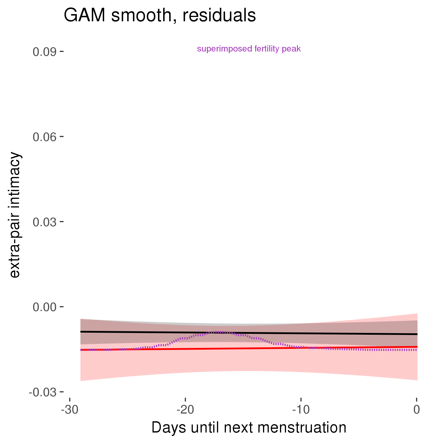
GAM smooth on raw data
As before, but without partialling anything out.
tryCatch({
  trend_plot = ggplot(tmp,aes_string(x = "RCD", y = outcome, colour = "included")) +
    stat_smooth(geom = 'smooth',size = 0.8, fill = "#9ECAE1", method = 'gam', formula = y ~ s(x))
}, error = function(e){cat_message(e, "danger")})

tryCatch({
  trend_data = ggplot_build(trend_plot)$data[[1]]
}, error = function(e){cat_message(e, "danger")})

trend_data$RCD = round(trend_data$x)
trend_data = left_join(trend_data, tmp %>% select(real, RCD,fertile) %>% unique(), by = "RCD")
trend_data %>%
  filter(real == TRUE) %>%
  mutate(superimposed = ( ( (fertile - 0.01)/0.58) * (max(y)-min(y) ) ) + min(y) ) ->
  trend_data

plot1b = ggplot(trend_data) +
  geom_ribbon(aes(x = x, ymin = ymin, ymax = ymax,  fill = factor(group)), alpha = 0.2) +
  geom_line(aes(x = x, y = y, colour = factor(group)), size = 0.8, stat = "identity") +
  scale_x_continuous(caption_x) +
  geom_line(aes(x = x, y = superimposed), color = "#a83fbf", size = 1, linetype = 'dashed') +
  annotate("text",x = mean(trend_data$x),  y = max(trend_data$superimposed,na.rm=T) + 0.1, label = 'superimposed fertility peak', color = "#a83fbf") +
  scale_y_continuous(outcome_label) +
  ggtitle("GAM smooth, raw data") +
  scale_color_manual("Contraception status",values = c("2"="black","1"= "red"), labels = c("2"="hormonally\ncontracepting","1"="cycling"), guide = F) +
  scale_fill_manual("Contraception status",values = c("2"="black","1"= "red"), labels = c("2"="hormonally\ncontracepting","1"="cycling"), guide = F)

suppressWarnings(print(plot1b))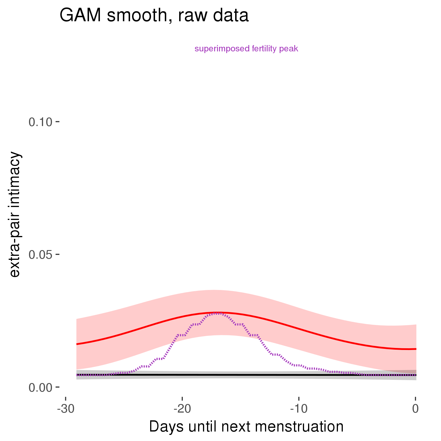
Means and standard errors over raw data
Nothing partialled out, just straight means with bootstrapped confidence intervals.
tryCatch({
  trend_plot = ggplot(tmp,aes_string(x = "RCD", y = outcome, colour = "included")) +
    geom_pointrange(size = 0.8, stat = 'summary', fun.data = "mean_cl_boot")
}, error = function(e){cat_message(e, "danger")})
tryCatch({
  trend_data = ggplot_build(trend_plot)$data[[1]]
}, error = function(e){cat_message(e, "danger")})

trend_data$RCD = round(trend_data$x)
trend_data = left_join(trend_data, tmp %>% select(real, RCD,fertile) %>% unique(), by = "RCD")
trend_data %>%
  filter(real == TRUE) %>%
  mutate(superimposed = ( ( (fertile - 0.01)/0.58) * (max(y)-min(y) ) ) + min(y) ) ->
  trend_data

plot3 = ggplot(trend_data) +
  geom_pointrange(aes(x = x, y = y, ymin = ymin,ymax = ymax, colour = factor(group)), size = 0.8, stat = "identity", alpha = 0.6, position = position_dodge(width = .5)) +
  scale_x_continuous("Days until next menstruation") +
  geom_line(aes(x= x, y = superimposed), color = "#a83fbf", size = 1, linetype = 'dashed') +
  annotate("text",x = mean(trend_data$x),  y = max(trend_data$superimposed,na.rm=T) + 0.1, label = 'superimposed fertility peak', color = "#a83fbf") +
  scale_y_continuous(outcome_label) +
  ggtitle("Means with standard errors, raw data") +
  scale_color_manual("Contraception status",values = c("2"="black","1"= "red"), labels = c("2"="hormonally\ncontracepting","1"="cycling"), guide = F) +
  scale_fill_manual("Contraception status",values = c("2"="black","1"= "red"), labels = c("2"="hormonally\ncontracepting","1"="cycling"), guide = F)
suppressWarnings(print(plot3))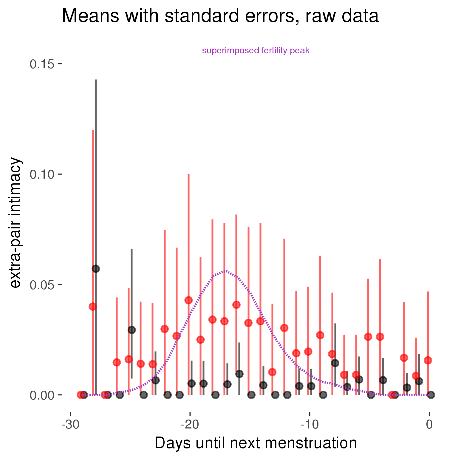
Forward-counted
model %>%
  plot_curve(diary %>% filter(minimum_cycle_length_diary <= 30, minimum_cycle_length_diary >= 27) %>% mutate(RCD = FCD, fertile = prc_stirn_b_forward_counted), caption_x = "Days since last menstruation")
outcome = names(model@frame)[1]
outcome_label = recode(str_replace_all(str_replace_all(str_replace_all(outcome, "_", " "), " pair", "-pair"), " 1", ""),
"desirability 1" = "self-perceived desirability",
"NARQ admiration" = "narcissistic admiration",
"NARQ rivalry" = "narcissistic rivalry",
"extra-pair" = "extra-pair desire & behaviour",
"had sexual intercourse" = "sexual intercourse")
library(ggplot2)
# form a subset and run the model without the hormonal contraception and the fertility predictors
tmp = diary %>%
filter(!is.na(fertile), !is.na(included),
RCD > -1 * minimum_cycle_length_diary, RCD > -40)
new_form = update.formula(formula(model), new = . ~ . - fertile * included)
tmp$residuals = residuals(update(model, new_form, data = tmp , na.action = na.exclude))
tmp = tmp %>%
filter(!is.na(RCD), !is.na(residuals))
rcd_min = min(tmp$RCD)
tmp$real = FALSE
tmp_before = tmp
tmp_before$RCD = tmp_before$RCD + min(tmp$RCD) - 1
tmp_after = tmp
tmp_after$RCD = tmp_after$RCD - min(tmp$RCD) + 1
tmp$real = TRUE
tmp = bind_rows(tmp_before %>% filter(RCD > rcd_min - 11), tmp, tmp_after %>% filter(RCD < 11))GAM smooth on residuals
Here, we partialled out menstruation and individual random effects, then superimposed estimated probability of being in the fertile window scaled to the range of the estimated means. To address the periodicity of the cycle, we prepended and appended ten days of the timeseries to the end and the beginning of the timeseries. We then estimated the GAM and cut off the appended subsets before plotting.
tryCatch({
  trend_plot = ggplot(tmp,aes(x = RCD, y = residuals, colour = included)) +
    stat_smooth(geom = 'smooth',size = 0.8, fill = "#9ECAE1", method = 'gam', formula = y ~ s(x))
}, error = function(e){cat_message(e, "danger")})

tryCatch({
  trend_data = ggplot_build(trend_plot)$data[[1]]
}, error = function(e){cat_message(e, "danger")})

trend_data$RCD = round(trend_data$x)
trend_data = left_join(trend_data, tmp %>% select(real, RCD,fertile) %>% unique(), by = "RCD")
trend_data %>%
  filter(real == TRUE) %>%
  mutate(superimposed = ( ( (fertile - 0.01)/0.58) * (max(y)-min(y) ) ) + min(y) ) ->
  trend_data


ggplot(trend_data) +
  geom_ribbon(aes(x = x, ymin = ymin, ymax = ymax,  fill = factor(group)), alpha = 0.2) +
  geom_line(aes(x = x, y = y, colour = factor(group)), size = 0.8, stat = "identity") +
  scale_x_continuous(caption_x) +
  geom_line(aes(x = x, y = superimposed), color = "#a83fbf", size = 1, linetype = 'dashed') +
  annotate("text",x = mean(trend_data$x),  y = max(trend_data$superimposed,na.rm=T) + 0.1, label = 'superimposed fertility peak', color = "#a83fbf") +
  scale_y_continuous(outcome_label) +
  ggtitle("GAM smooth, residuals") +
  scale_color_manual("Contraception status",values = c("2"="black","1"= "red"), labels = c("2"="hormonally\ncontracepting","1"="cycling"), guide = F) +
  scale_fill_manual("Contraception status",values = c("2"="black","1"= "red"), labels = c("2"="hormonally\ncontracepting","1"="cycling"), guide = F)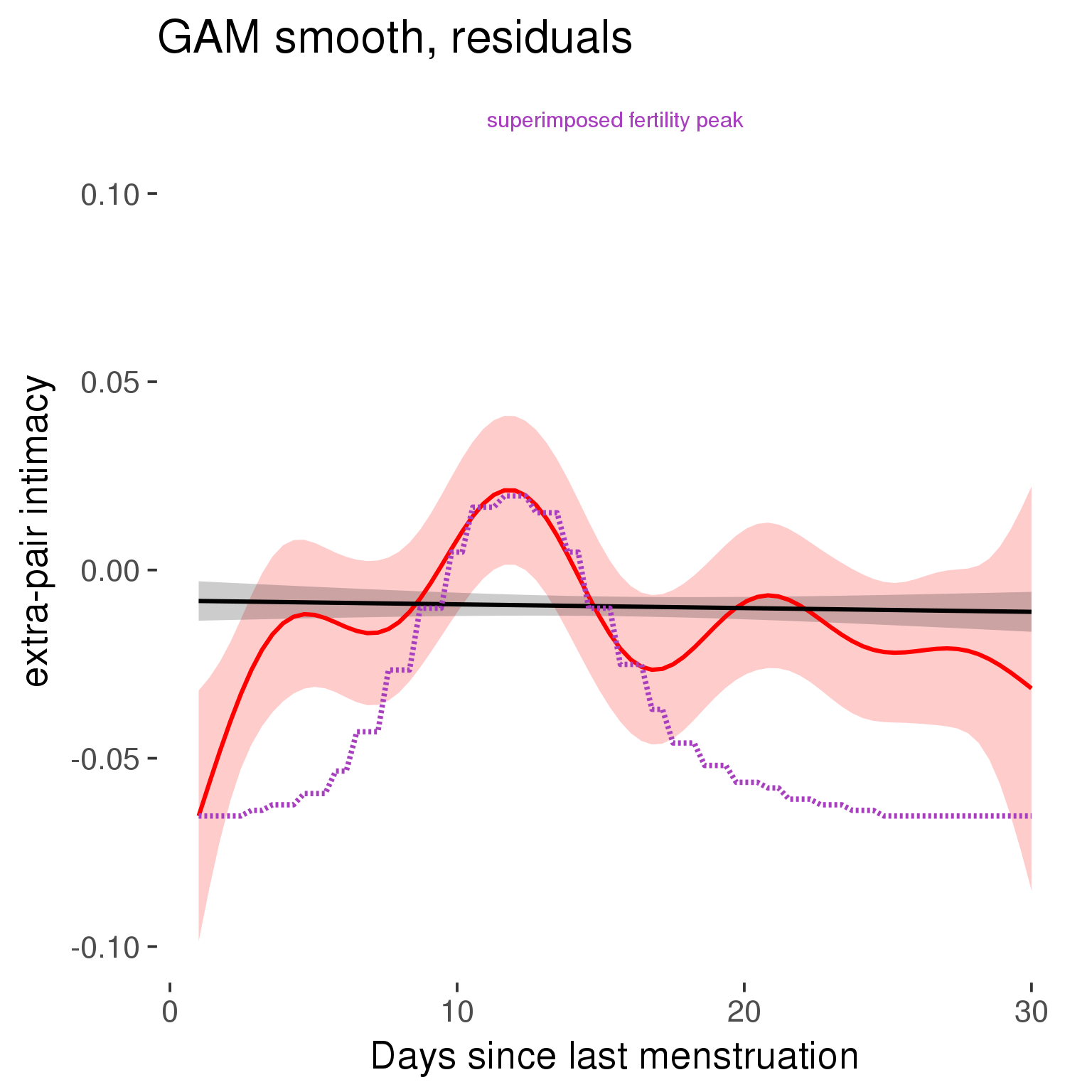
GAM smooth on raw data
As before, but without partialling anything out.
tryCatch({
  trend_plot = ggplot(tmp,aes_string(x = "RCD", y = outcome, colour = "included")) +
    stat_smooth(geom = 'smooth',size = 0.8, fill = "#9ECAE1", method = 'gam', formula = y ~ s(x))
}, error = function(e){cat_message(e, "danger")})

tryCatch({
  trend_data = ggplot_build(trend_plot)$data[[1]]
}, error = function(e){cat_message(e, "danger")})

trend_data$RCD = round(trend_data$x)
trend_data = left_join(trend_data, tmp %>% select(real, RCD,fertile) %>% unique(), by = "RCD")
trend_data %>%
  filter(real == TRUE) %>%
  mutate(superimposed = ( ( (fertile - 0.01)/0.58) * (max(y)-min(y) ) ) + min(y) ) ->
  trend_data

plot1b = ggplot(trend_data) +
  geom_ribbon(aes(x = x, ymin = ymin, ymax = ymax,  fill = factor(group)), alpha = 0.2) +
  geom_line(aes(x = x, y = y, colour = factor(group)), size = 0.8, stat = "identity") +
  scale_x_continuous(caption_x) +
  geom_line(aes(x = x, y = superimposed), color = "#a83fbf", size = 1, linetype = 'dashed') +
  annotate("text",x = mean(trend_data$x),  y = max(trend_data$superimposed,na.rm=T) + 0.1, label = 'superimposed fertility peak', color = "#a83fbf") +
  scale_y_continuous(outcome_label) +
  ggtitle("GAM smooth, raw data") +
  scale_color_manual("Contraception status",values = c("2"="black","1"= "red"), labels = c("2"="hormonally\ncontracepting","1"="cycling"), guide = F) +
  scale_fill_manual("Contraception status",values = c("2"="black","1"= "red"), labels = c("2"="hormonally\ncontracepting","1"="cycling"), guide = F)

suppressWarnings(print(plot1b))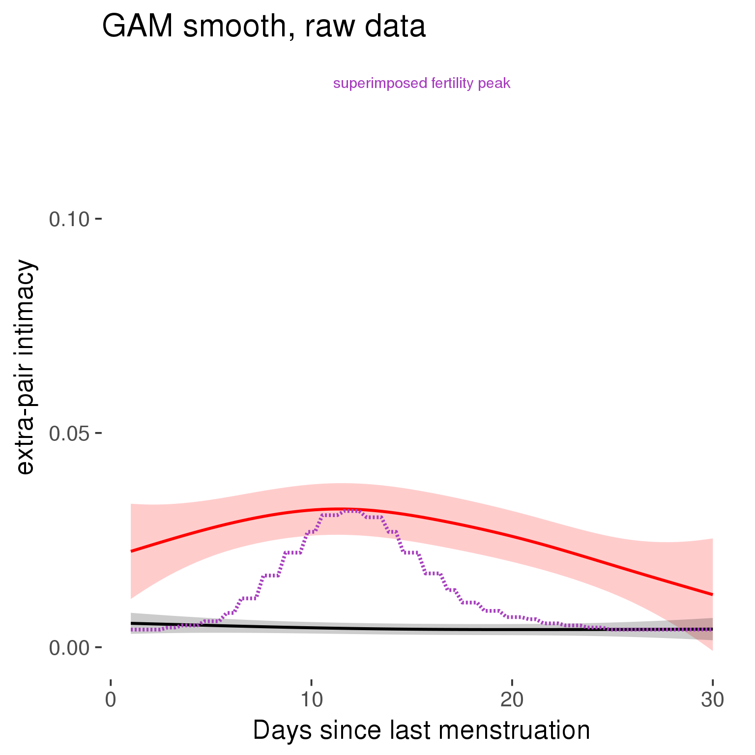
Means and standard errors over raw data
Nothing partialled out, just straight means with bootstrapped confidence intervals.
tryCatch({
  trend_plot = ggplot(tmp,aes_string(x = "RCD", y = outcome, colour = "included")) +
    geom_pointrange(size = 0.8, stat = 'summary', fun.data = "mean_cl_boot")
}, error = function(e){cat_message(e, "danger")})
tryCatch({
  trend_data = ggplot_build(trend_plot)$data[[1]]
}, error = function(e){cat_message(e, "danger")})

trend_data$RCD = round(trend_data$x)
trend_data = left_join(trend_data, tmp %>% select(real, RCD,fertile) %>% unique(), by = "RCD")
trend_data %>%
  filter(real == TRUE) %>%
  mutate(superimposed = ( ( (fertile - 0.01)/0.58) * (max(y)-min(y) ) ) + min(y) ) ->
  trend_data

plot3 = ggplot(trend_data) +
  geom_pointrange(aes(x = x, y = y, ymin = ymin,ymax = ymax, colour = factor(group)), size = 0.8, stat = "identity", alpha = 0.6, position = position_dodge(width = .5)) +
  scale_x_continuous("Days until next menstruation") +
  geom_line(aes(x= x, y = superimposed), color = "#a83fbf", size = 1, linetype = 'dashed') +
  annotate("text",x = mean(trend_data$x),  y = max(trend_data$superimposed,na.rm=T) + 0.1, label = 'superimposed fertility peak', color = "#a83fbf") +
  scale_y_continuous(outcome_label) +
  ggtitle("Means with standard errors, raw data") +
  scale_color_manual("Contraception status",values = c("2"="black","1"= "red"), labels = c("2"="hormonally\ncontracepting","1"="cycling"), guide = F) +
  scale_fill_manual("Contraception status",values = c("2"="black","1"= "red"), labels = c("2"="hormonally\ncontracepting","1"="cycling"), guide = F)
suppressWarnings(print(plot3))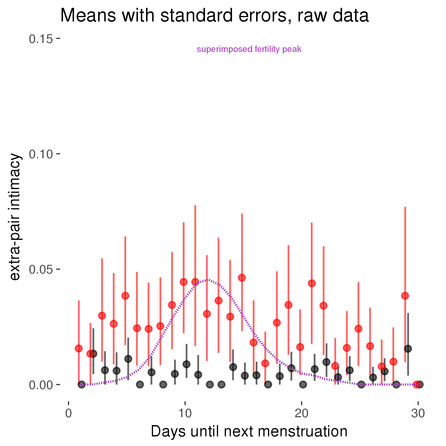
Robustness checks
M_r1: Random slopes for conception risk and menstruation
tryCatch({
# refit model with random effects for fertile and menstruation dummies
with_ind_diff = update(model, formula = . ~ . - (1| person) + (1 + fertile + menstruation | person))

# pull the random effects, format as tibble
rand = coef(with_ind_diff)$person %>%
  tibble::rownames_to_column("person") %>%
  mutate(person = as.numeric(person))

# pull the fixed effects
fixd = data.frame(fixef(with_ind_diff)) %>%
  tibble::rownames_to_column("effect")
names(fixd) = c("effect", "pop_effect_size")

# pull apart the coefficients so that we can account for the fact that the random effect variation implicitly includes HC explaining the mean population-level effect of fertile/menstruation dummies among HC users
fixd = fixd %>%
  separate(effect, c("included", "effect"), sep = ":", fill = "left") %>%
  mutate(included = if_else(is.na(included), "cycling", str_replace(included, "included", "")))
fixd[2,c("included", "effect")] = c("horm_contra", "(Intercept)")


rand = rand %>%
  # merge diary data on the random effects, so that we know who is a HC users and who isn't
  inner_join(diary %>% select(person, included) %>% unique(), by = 'person') %>%
  # gather into long format, to have the dataset by predictor
  gather(effect, value, -person, -included) %>%
  inner_join(fixd, by = c('effect', 'included')) %>%
  # pull the fixed effects
  mutate(
    # only for those who are HC users, add the moderated population effect size for this effect (the random effects have the reference category mean)
    value = if_else(included == "horm_contra", value + pop_effect_size, value),
    effect = recode(effect, "includedhorm_contra" = "HC user",
                   "includedhorm_contra:fertile" = "HC user x fertile",
                   "includedhorm_contra:menstruationpre" = "HC user x premens.",
                   "includedhorm_contra:menstruationyes" = "HC user x mens.",
                   "menstruationyes" = "mens.",
                   "menstruationpre" = "premens.")) %>%
  group_by(included, effect) %>%
  # filter out predictors that aren't modelled as varying/random
  filter(sd(value) > 0)

# plot dot plot of random effects
print(
ggplot(rand, aes(x = included, y = value, color = included, fill = included)) +
  facet_wrap( ~ effect, scales = "free") +
  # geom_violin(alpha = 0.4, size = 0) +
  geom_dotplot(binaxis='y', dotsize = 0.1, method = "histodot") +
# geom_jitter(alpha = 0.05) +
  coord_flip() +
  geom_pointrange(stat = 'summary', fun.data = 'mean_sdl', color = 'darkred', size = 1.2) +
  scale_color_manual("Contraception status", values = c("horm_contra"="black","cycling"= "red"), labels = c("horm_contra"="hormonally\ncontracepting","cycling"="cycling"), guide = F) +
  scale_fill_manual("Contraception status", values = c("horm_contra"="black","cycling"= "red"), labels = c("horm_contra"="hormonally\ncontracepting","1"="cycling"), guide = F) +
  ggtitle("M_r1: allowing participant-varying slopes", subtitle = "for the conception risk measure and the menstruation dummies") +
  scale_x_discrete("Hormonal contraception", breaks = c("horm_contra", "cycling"), labels = c("yes", "no")) +
  scale_y_continuous("Random effect size distribution"))

print_summary(with_ind_diff)
cat(pander(anova(model, with_ind_diff)))
}, error = function(e){
  with_ind_diff = model
  cat_message(e, "danger")
})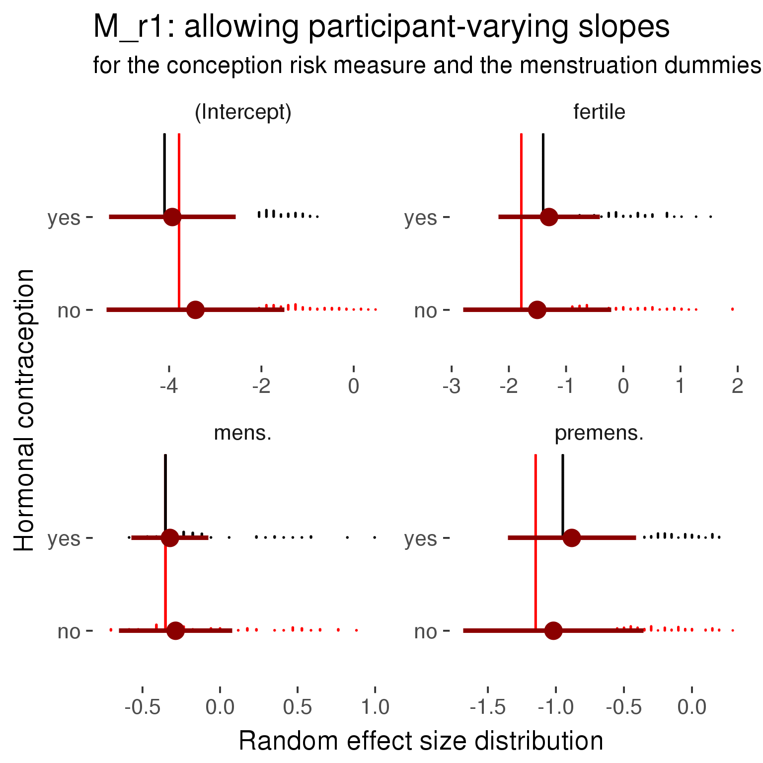
Generalized linear mixed model fit by maximum likelihood (Laplace Approximation) ['glmerMod']
 Family: binomial  ( probit )
Formula: extra_pair_intimacy ~ included + menstruation + fertile + fertile_mean +
    (1 + fertile + menstruation | person) + included:menstruation +      included:fertile
   Data: diary

     AIC      BIC   logLik deviance df.resid
    2399     2555    -1181     2361    26684

Scaled residuals:
   Min     1Q Median     3Q    Max
-2.607 -0.004 -0.002 -0.001  6.512

Random effects:
 Groups Name            Variance Std.Dev. Corr
 person (Intercept)     5.507    2.347
        fertile         3.607    1.899    0.72
        menstruationpre 0.683    0.827    0.98 0.57
        menstruationyes 0.614    0.783    0.24 0.27 0.18
Number of obs: 26703, groups:  person, 1054

Fixed effects:
                                     Estimate Std. Error z value Pr(>|z|)
(Intercept)                         -3.803110   0.000463   -8212   <2e-16 ***
includedhorm_contra                 -0.321515   0.000463    -694   <2e-16 ***
menstruationpre                     -1.145626   0.000463   -2474   <2e-16 ***
menstruationyes                     -0.325812   0.000463    -704   <2e-16 ***
fertile                             -1.731209   0.000463   -3739   <2e-16 ***
fertile_mean                        -0.104871   0.000463    -227   <2e-16 ***
includedhorm_contra:menstruationpre  0.196076   0.000463     424   <2e-16 ***
includedhorm_contra:menstruationyes -0.018182   0.000463     -39   <2e-16 ***
includedhorm_contra:fertile          0.314216   0.000463     679   <2e-16 ***
---
Signif. codes:  0 '***' 0.001 '**' 0.01 '*' 0.05 '.' 0.1 ' ' 1

Correlation of Fixed Effects:
                        (Intr) incld_ mnstrtnp mnstrtny fertil frtl_m inclddhrm_cntr:mnstrtnp
inclddhrm_c             0.000
menstrutnpr             0.000  0.000
menstrutnys             0.000  0.000  0.000
fertile                 0.000  0.000  0.000    0.000
fertile_men             0.000  0.000  0.000    0.000    0.000
inclddhrm_cntr:mnstrtnp 0.000  0.000  0.000    0.000    0.000  0.000
inclddhrm_cntr:mnstrtny 0.000  0.000  0.000    0.000    0.000  0.000  0.000
inclddhrm_cntr:f        0.000  0.000  0.000    0.000    0.000  0.000  0.000
                        inclddhrm_cntr:mnstrtny
inclddhrm_c
menstrutnpr
menstrutnys
fertile
fertile_men
inclddhrm_cntr:mnstrtnp
inclddhrm_cntr:mnstrtny
inclddhrm_cntr:f        0.000
convergence code: 0
Model failed to converge with max|grad| = 0.154676 (tol = 0.001, component 1)
Model is nearly unidentifiable: very large eigenvalue
 - Rescale variables?
| Df | AIC | BIC | logLik | deviance | Chisq | Chi Df | Pr(>Chisq) | |
|---|---|---|---|---|---|---|---|---|
| model | 10 | 2387 | 2469 | -1184 | 2367 | NA | NA | NA |
| with_ind_diff | 19 | 2399 | 2555 | -1181 | 2361 | 5.628 | 9 | 0.7765 |
robustness_check_ovu_shift(model, diary)Error: Error in pwrssUpdate(pp, resp, tol = tolPwrss, GQmat = GQmat, compDev = compDev, : Downdated VtV is not positive definite
Error: Error in pwrssUpdate(pp, resp, tol = tolPwrss, GQmat = GQmat, compDev = compDev, : (maxstephalfit) PIRLS step-halvings failed to reduce deviance in pwrssUpdate
Error: Error in pwrssUpdate(pp, resp, tol = tolPwrss, GQmat = GQmat, compDev = compDev, : (maxstephalfit) PIRLS step-halvings failed to reduce deviance in pwrssUpdate
M_e: Exclusion criteria
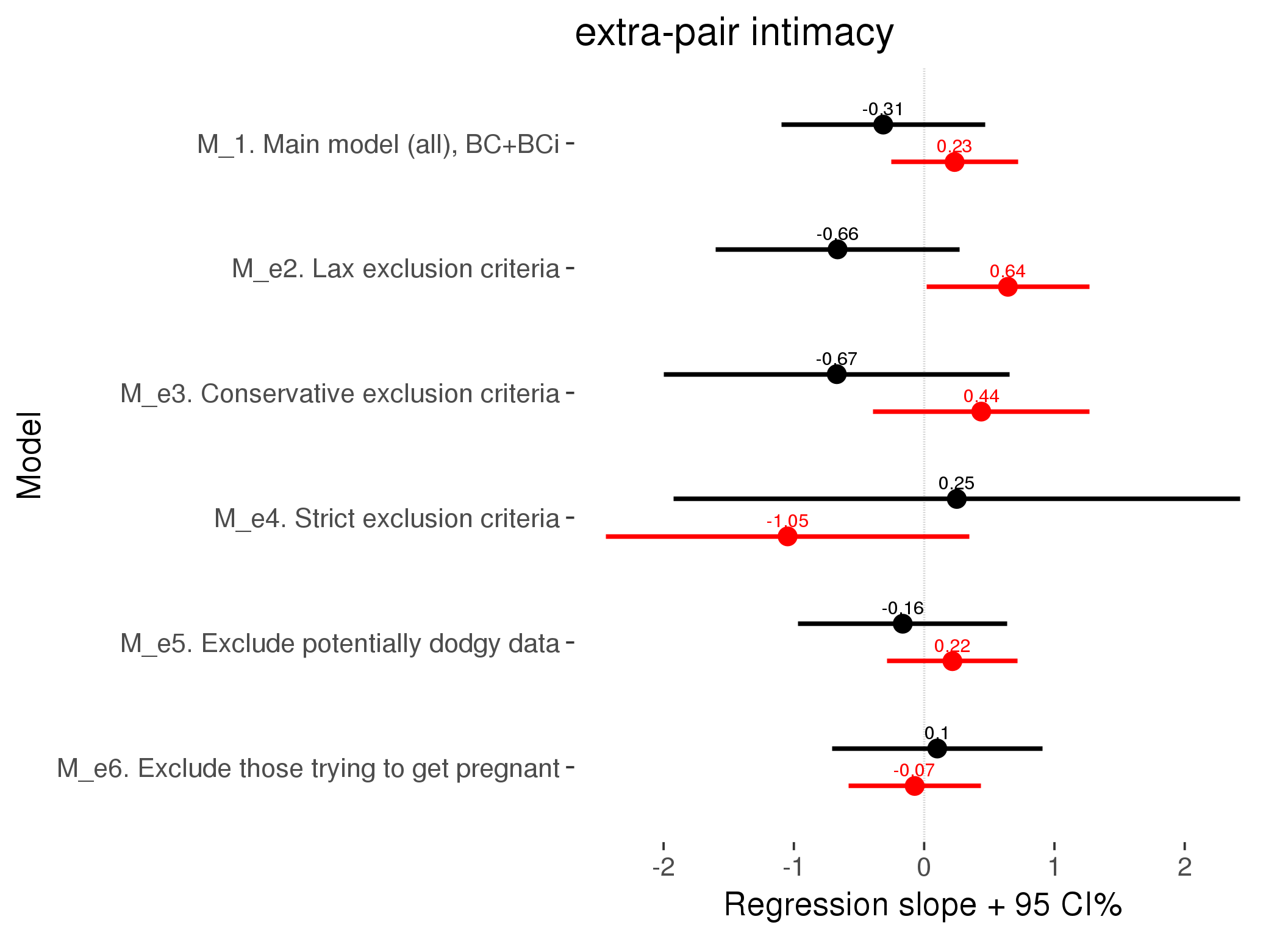
M_p: Predictors
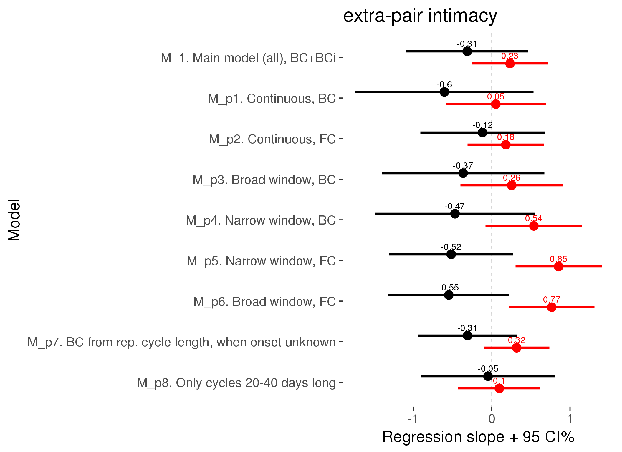
M_c: Covariates, controls, autocorrelation
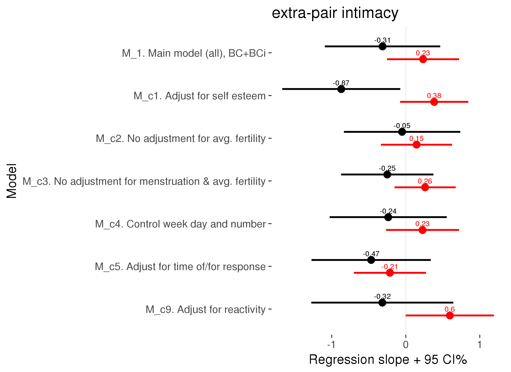
Generalized linear mixed model fit by maximum likelihood (Laplace Approximation) ['glmerMod']
 Family: binomial  ( probit )

     AIC      BIC   logLik deviance df.resid
  1985.5   2131.3   -974.7   1949.5    24379

Scaled residuals:
   Min     1Q Median     3Q    Max
-2.024 -0.003 -0.002 -0.002  7.219

Random effects:
 Groups Name                                   Variance Std.Dev.
 person (Intercept)                            7.7216   2.779
 Xr.2   s(days_filled_out):includedhorm_contra 0.0641   0.253
 Xr.1   s(days_filled_out):includedcycling     0.0469   0.217
 Xr.0   s(day_number):includedhorm_contra      0.0726   0.269
 Xr     s(day_number):includedcycling          0.0125   0.112
Number of obs: 24397, groups:  person, 1054; Xr.2, 8; Xr.1, 8; Xr.0, 8; Xr, 8

Fixed effects:
                                           Estimate Std. Error z value     Pr(>|z|)
X(Intercept)                                -4.0997     0.6753   -6.07 0.0000000013 ***
Xincludedhorm_contra                        -0.0854     0.5477   -0.16         0.88
Xmenstruationpre                             0.1767     0.1418    1.25         0.21
Xmenstruationyes                             0.0712     0.1429    0.50         0.62
Xfertile                                     0.5954     0.3042    1.96         0.05 .
Xfertile_mean                               -2.2201     3.5303   -0.63         0.53
Xincludedhorm_contra:menstruationpre        -0.2491     0.2459   -1.01         0.31
Xincludedhorm_contra:menstruationyes        -0.0396     0.2380   -0.17         0.87
Xincludedhorm_contra:fertile                -0.3167     0.4892   -0.65         0.52
Xs(day_number):includedcyclingFx1            0.2171     0.2466    0.88         0.38
Xs(day_number):includedhorm_contraFx1       -0.0190     0.3338   -0.06         0.95
Xs(days_filled_out):includedcyclingFx1      -0.1549     0.2641   -0.59         0.56
Xs(days_filled_out):includedhorm_contraFx1   0.0227     0.3400    0.07         0.95
---
Signif. codes:  0 '***' 0.001 '**' 0.01 '*' 0.05 '.' 0.1 ' ' 1
Family: binomial
Link function: probit

Formula:
extra_pair_intimacy ~ included + menstruation + fertile + fertile_mean +
    s(day_number, by = included) + s(days_filled_out, by = included) +
    included:menstruation + included:fertile

Parametric coefficients:
                                    Estimate Std. Error z value     Pr(>|z|)
(Intercept)                          -4.0997     0.6754   -6.07 0.0000000013 ***
includedhorm_contra                  -0.0854     0.5477   -0.16         0.88
menstruationpre                       0.1767     0.1418    1.25         0.21
menstruationyes                       0.0712     0.1429    0.50         0.62
fertile                               0.5954     0.3042    1.96         0.05 .
fertile_mean                         -2.2201     3.5304   -0.63         0.53
includedhorm_contra:menstruationpre  -0.2491     0.2459   -1.01         0.31
includedhorm_contra:menstruationyes  -0.0396     0.2380   -0.17         0.87
includedhorm_contra:fertile          -0.3167     0.4892   -0.65         0.52
---
Signif. codes:  0 '***' 0.001 '**' 0.01 '*' 0.05 '.' 0.1 ' ' 1

Approximate significance of smooth terms:
                                        edf Ref.df Chi.sq p-value
s(day_number):includedcycling          1.16   1.16   0.69    0.42
s(day_number):includedhorm_contra      1.47   1.47   0.10    0.90
s(days_filled_out):includedcycling     1.52   1.52   1.30    0.54
s(days_filled_out):includedhorm_contra 1.39   1.39   0.03    0.95

R-sq.(adj) =  -0.000547
glmer.ML = 1434.9  Scale est. = 1         n = 24397
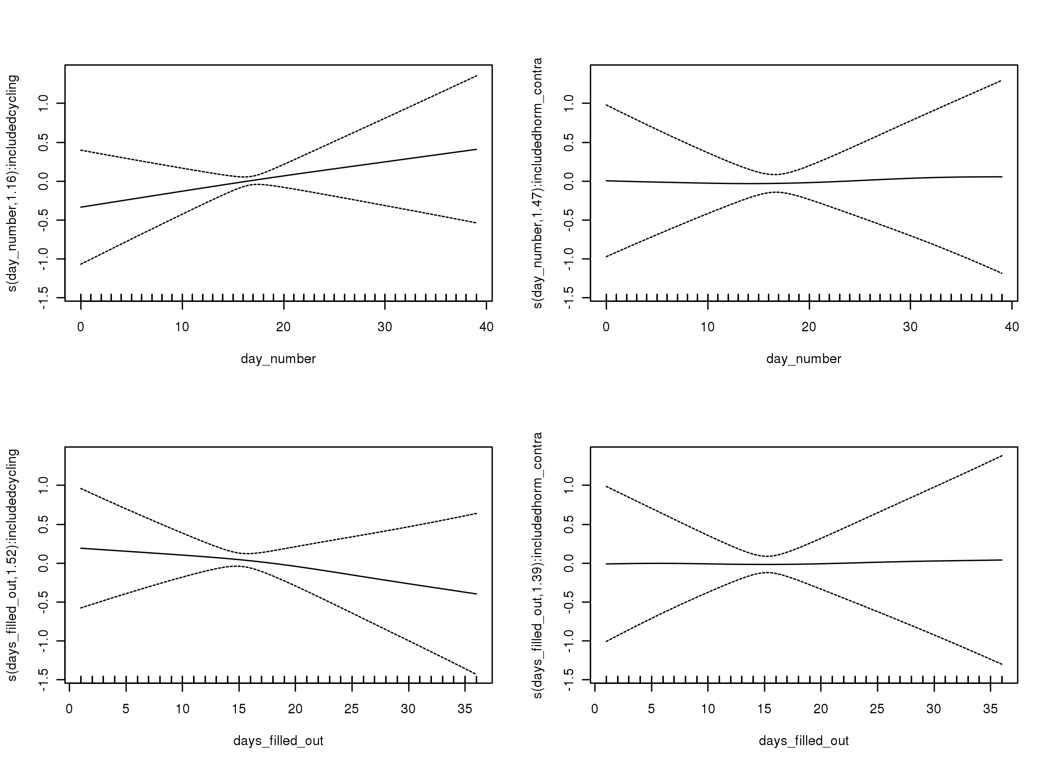
M_d: Other designs
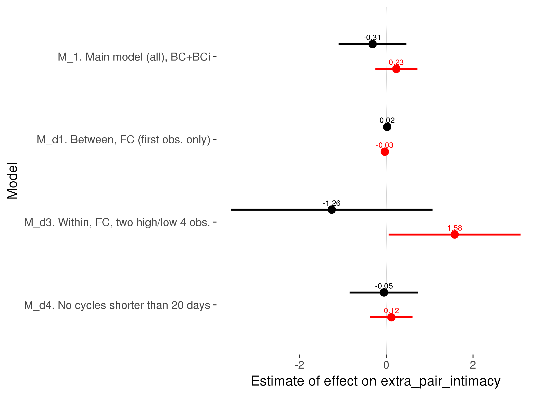
M_m1: Moderation by contraceptive method
Based on the sample with lax exclusion criteria. Users who used any hormonal contraception are classified as hormonal, users who use any awareness-based methods (counting, temperature-based) are classified as ‘fertility-awareness’, women who don’t fall into the before groups and use condoms, pessars, coitus interruptus etc. are classified as ‘barrie or abstinence’. Women who don’t use contraception or use other methods such as sterilisation are excluded from this analysis.
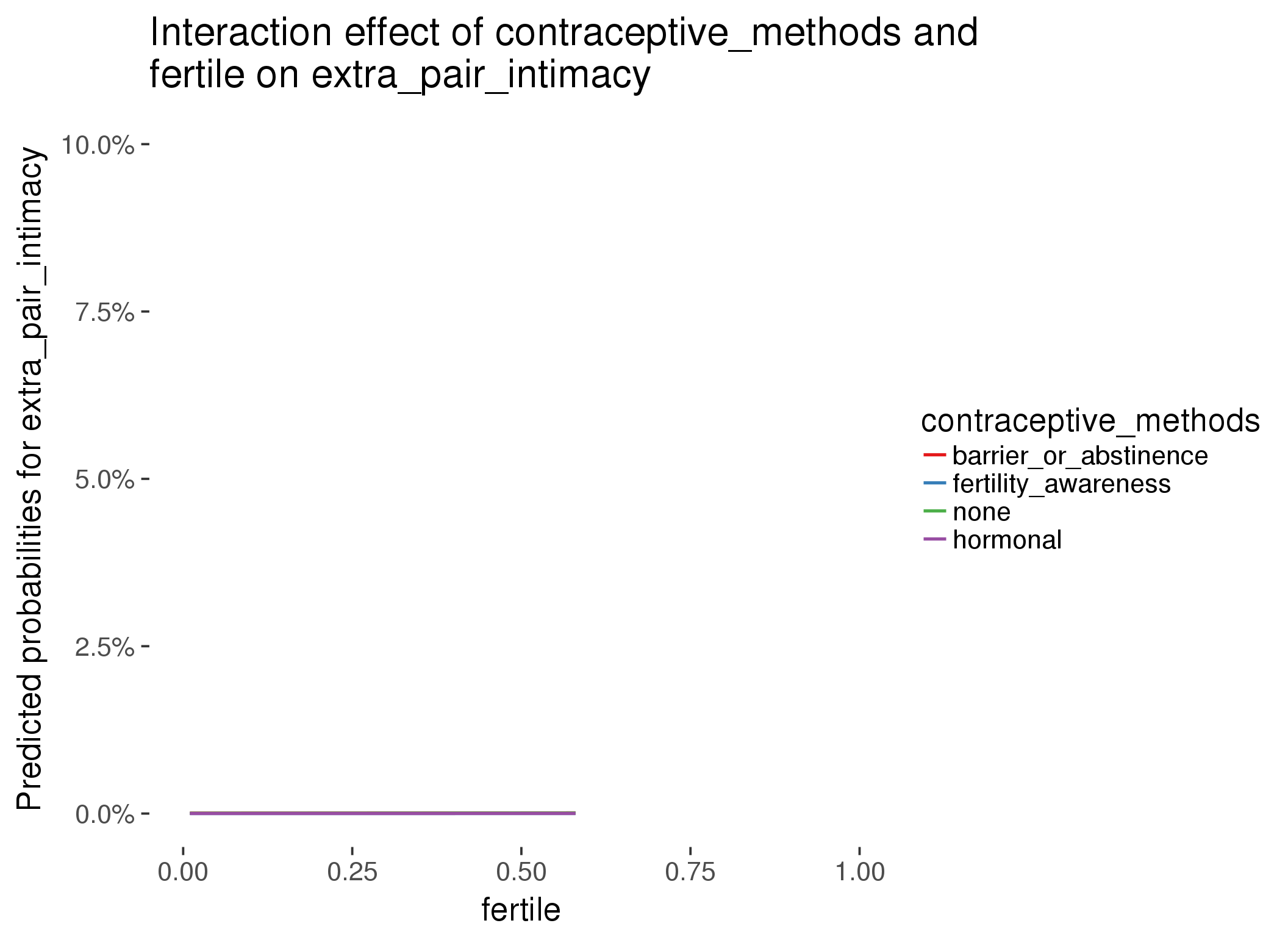
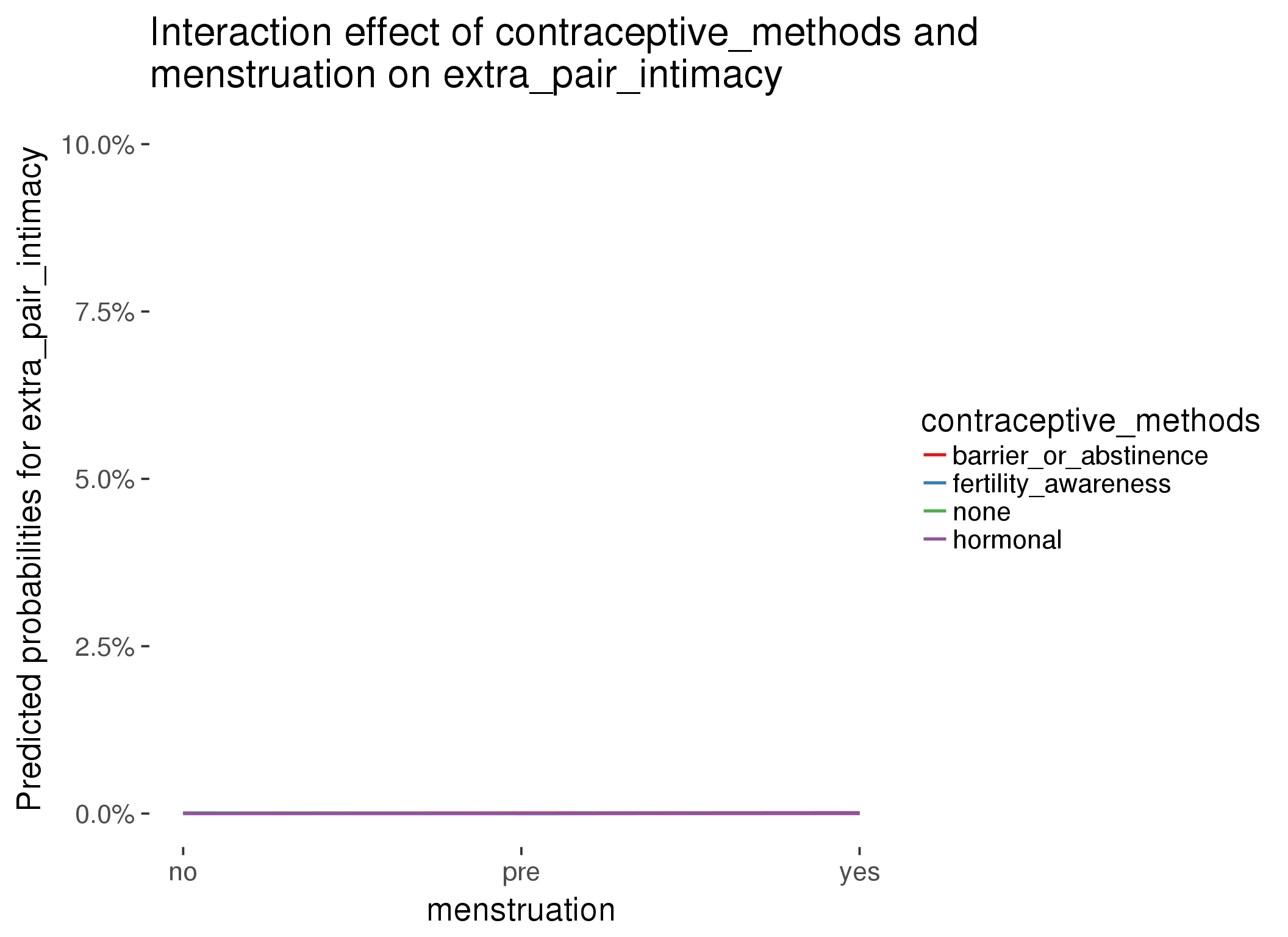
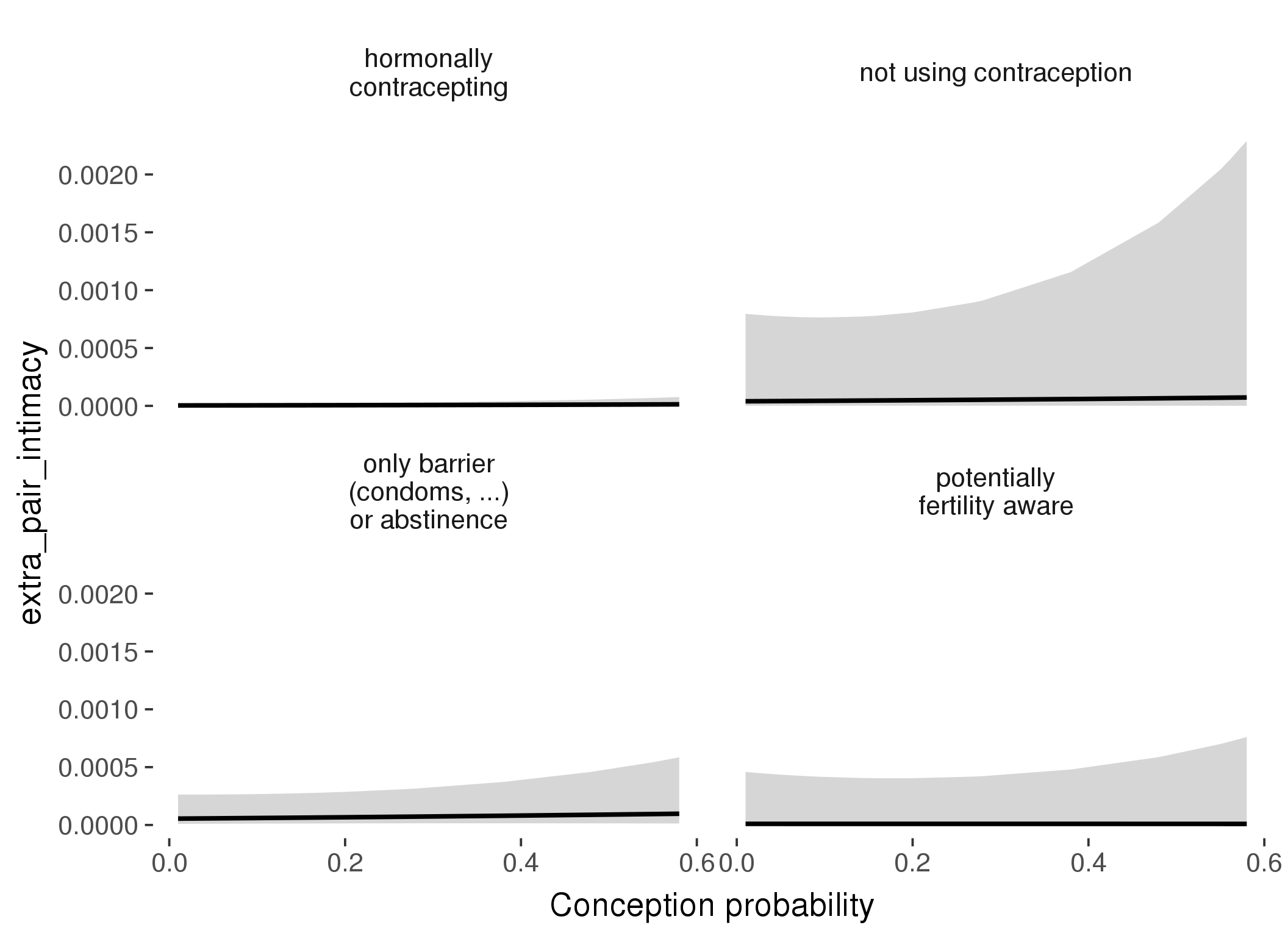
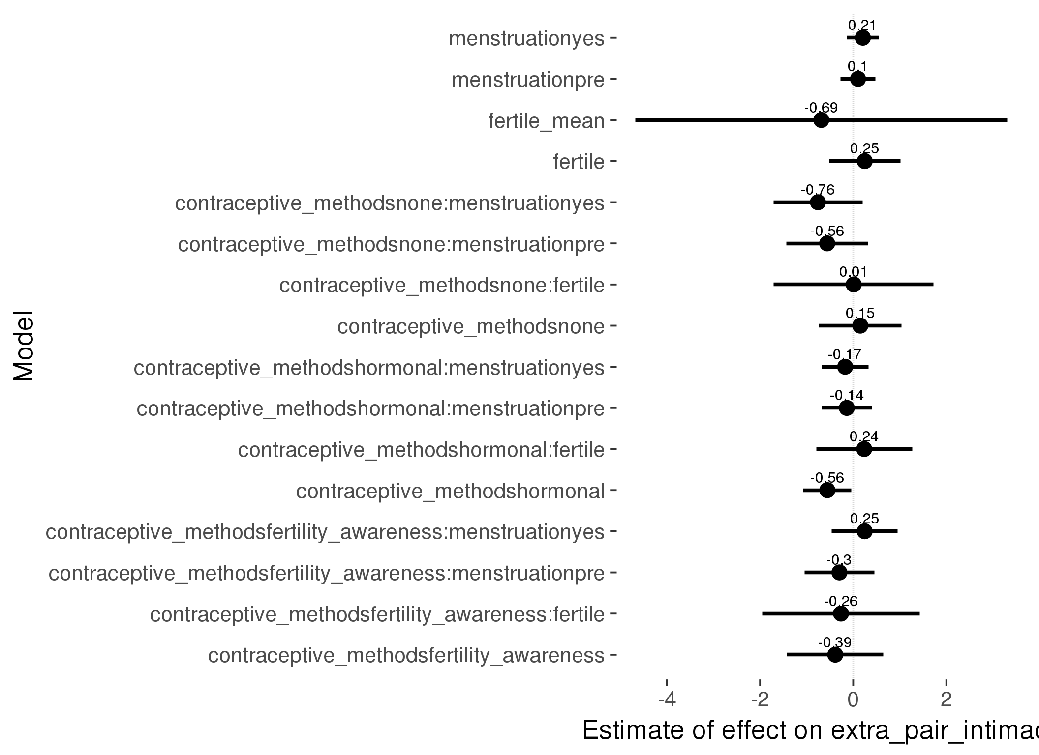
Generalized linear mixed model fit by maximum likelihood (Laplace Approximation) ['glmerMod']
 Family: binomial  ( probit )
Formula: extra_pair_intimacy ~ fertile_mean + (1 | person) + contraceptive_methods +
    fertile + menstruation + fertile:contraceptive_methods +      menstruation:contraceptive_methods
   Data: diary
 Subset: !is.na(included_lax) & contraceptive_method != "other"

     AIC      BIC   logLik deviance df.resid
  1541.8   1681.2   -752.9   1505.8    17026

Scaled residuals:
   Min     1Q Median     3Q    Max
-2.033 -0.007 -0.003 -0.002  7.897

Random effects:
 Groups Name        Variance Std.Dev.
 person (Intercept) 4.68     2.16
Number of obs: 17044, groups:  person, 513

Fixed effects:
                                                         Estimate Std. Error z value Pr(>|z|)
(Intercept)                                              -3.80264    0.40453   -9.40   <2e-16 ***
fertile_mean                                             -0.68606    2.03840   -0.34    0.736
contraceptive_methodsfertility_awareness                 -0.38619    0.52850   -0.73    0.465
contraceptive_methodsnone                                 0.15123    0.45224    0.33    0.738
contraceptive_methodshormonal                            -0.55661    0.26429   -2.11    0.035 *
fertile                                                   0.24713    0.39099    0.63    0.527
menstruationpre                                           0.10249    0.18946    0.54    0.589
menstruationyes                                           0.20636    0.17425    1.18    0.236
contraceptive_methodsfertility_awareness:fertile         -0.26345    0.86505   -0.30    0.761
contraceptive_methodsnone:fertile                         0.00997    0.87654    0.01    0.991
contraceptive_methodshormonal:fertile                     0.23538    0.52652    0.45    0.655
contraceptive_methodsfertility_awareness:menstruationpre -0.29696    0.38205   -0.78    0.437
contraceptive_methodsnone:menstruationpre                -0.55985    0.44830   -1.25    0.212
contraceptive_methodshormonal:menstruationpre            -0.13800    0.27313   -0.51    0.613
contraceptive_methodsfertility_awareness:menstruationyes  0.24577    0.36205    0.68    0.497
contraceptive_methodsnone:menstruationyes                -0.75828    0.48724   -1.56    0.120
contraceptive_methodshormonal:menstruationyes            -0.17371    0.25557   -0.68    0.497
---
Signif. codes:  0 '***' 0.001 '**' 0.01 '*' 0.05 '.' 0.1 ' ' 1
convergence code: 0
Model failed to converge with max|grad| = 2.48122 (tol = 0.001, component 1)
| Df | AIC | BIC | logLik | deviance | Chisq | Chi Df | Pr(>Chisq) | |
|---|---|---|---|---|---|---|---|---|
| add_main | 12 | 1527 | 1620 | -751.4 | 1503 | NA | NA | NA |
| by_method | 18 | 1542 | 1681 | -752.9 | 1506 | 0 | 6 | 1 |
M_m2: Moderation by participant age
model %>%
test_moderator("age_group", diary, xlevels = 5)| Df | AIC | BIC | logLik | deviance | Chisq | Chi Df | Pr(>Chisq) | |
|---|---|---|---|---|---|---|---|---|
| with_main | 18 | 2417 | 2565 | -1191 | 2381 | NA | NA | NA |
| with_mod | 26 | 2418 | 2631 | -1183 | 2366 | 15.69 | 8 | 0.04706 |
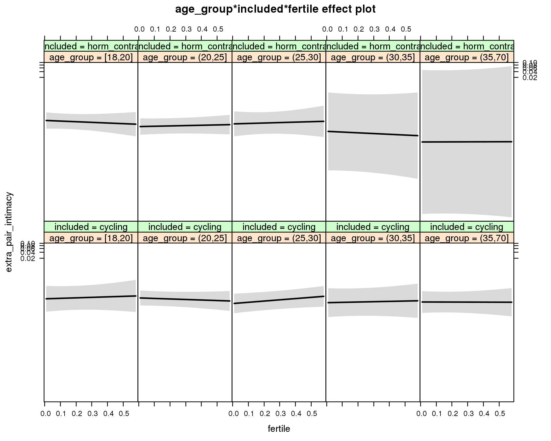
Generalized linear mixed model fit by maximum likelihood (Laplace Approximation) ['glmerMod']
 Family: binomial  ( probit )
Formula: extra_pair_intimacy ~ menstruation + fertile_mean + (1 | person) +
    age_group + included + fertile + menstruation:included +
    age_group:included + age_group:fertile + included:fertile +      age_group:included:fertile
   Data: diary

     AIC      BIC   logLik deviance df.resid
    2418     2631    -1183     2366    26677

Scaled residuals:
   Min     1Q Median     3Q    Max
-2.011 -0.003 -0.002 -0.002  8.212

Random effects:
 Groups Name        Variance Std.Dev.
 person (Intercept) 6.84     2.62
Number of obs: 26703, groups:  person, 1054

Fixed effects:
                                             Estimate Std. Error z value Pr(>|z|)
(Intercept)                                   -3.9368     0.4004   -9.83   <2e-16 ***
menstruationpre                               -0.0614     0.1208   -0.51     0.61
menstruationyes                                0.0388     0.1127    0.34     0.73
fertile_mean                                  -1.2594     1.3600   -0.93     0.35
age_group(20,25]                               0.0471     0.3751    0.13     0.90
age_group(25,30]                              -0.2444     0.4087   -0.60     0.55
age_group(30,35]                              -0.1997     0.4947   -0.40     0.69
age_group(35,70]                              -0.1637     0.4304   -0.38     0.70
includedhorm_contra                           -0.0857     0.3978   -0.22     0.83
fertile                                        0.2553     0.7189    0.36     0.72
menstruationpre:includedhorm_contra           -0.1462     0.2115   -0.69     0.49
menstruationyes:includedhorm_contra           -0.0654     0.1908   -0.34     0.73
age_group(20,25]:includedhorm_contra          -0.3667     0.4705   -0.78     0.44
age_group(25,30]:includedhorm_contra           0.0639     0.5595    0.11     0.91
age_group(30,35]:includedhorm_contra          -0.3654     1.1436   -0.32     0.75
age_group(35,70]:includedhorm_contra          -0.9536     1.9402   -0.49     0.62
age_group(20,25]:fertile                      -0.5267     0.8098   -0.65     0.52
age_group(25,30]:fertile                       0.3874     0.8058    0.48     0.63
age_group(30,35]:fertile                      -0.0859     0.9749   -0.09     0.93
age_group(35,70]:fertile                      -0.2771     0.9255   -0.30     0.76
includedhorm_contra:fertile                   -0.5902     0.9213   -0.64     0.52
age_group(20,25]:includedhorm_contra:fertile   1.0349     1.0542    0.98     0.33
age_group(25,30]:includedhorm_contra:fertile   0.1775     1.2718    0.14     0.89
age_group(30,35]:includedhorm_contra:fertile   0.0352     1.6152    0.02     0.98
age_group(35,70]:includedhorm_contra:fertile   0.6360     1.7951    0.35     0.72
---
Signif. codes:  0 '***' 0.001 '**' 0.01 '*' 0.05 '.' 0.1 ' ' 1
convergence code: 0
Model failed to converge with max|grad| = 2.26747 (tol = 0.001, component 1)
failure to converge in 10000 evaluations
M_m3: Moderation by weekend
model %>%
test_moderator("weekend", diary, xlevels = 2) | Df | AIC | BIC | logLik | deviance | Chisq | Chi Df | Pr(>Chisq) | |
|---|---|---|---|---|---|---|---|---|
| with_main | 12 | 2396 | 2494 | -1186 | 2372 | NA | NA | NA |
| with_mod | 14 | 2408 | 2523 | -1190 | 2380 | 0 | 2 | 1 |
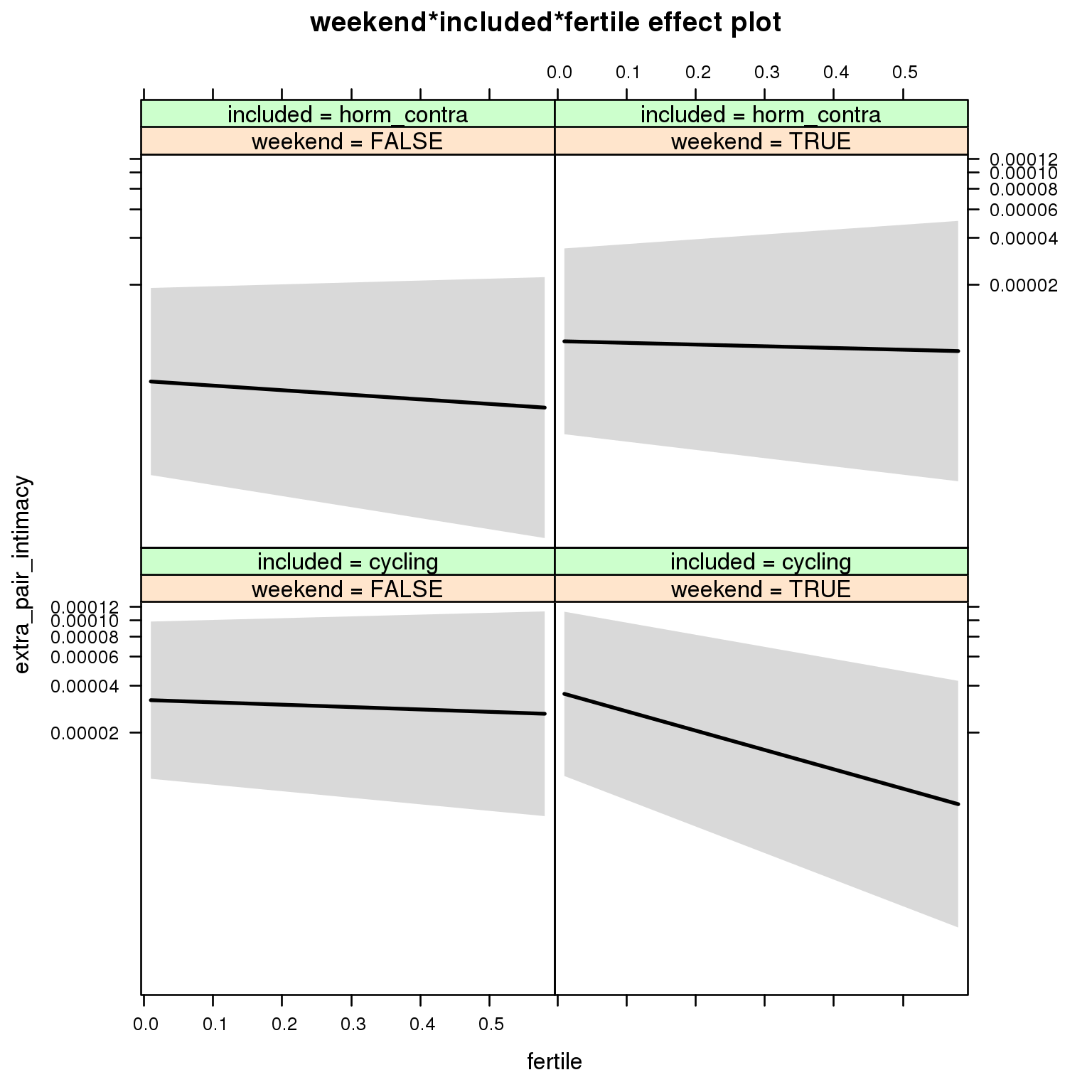
Generalized linear mixed model fit by maximum likelihood (Laplace Approximation) ['glmerMod']
 Family: binomial  ( probit )
Formula: extra_pair_intimacy ~ menstruation + fertile_mean + (1 | person) +
    weekend + included + fertile + menstruation:included + weekend:included +
    weekend:fertile + included:fertile + weekend:included:fertile
   Data: diary

     AIC      BIC   logLik deviance df.resid
    2408     2523    -1190     2380    26689

Scaled residuals:
   Min     1Q Median     3Q    Max
-2.078 -0.005 -0.003 -0.002  8.707

Random effects:
 Groups Name        Variance Std.Dev.
 person (Intercept) 4.7      2.17
Number of obs: 26703, groups:  person, 1054

Fixed effects:
                                        Estimate Std. Error z value Pr(>|z|)
(Intercept)                              -3.6002     0.2332  -15.44   <2e-16 ***
menstruationpre                          -0.2011     0.1172   -1.72    0.086 .
menstruationyes                          -0.2002     0.1129   -1.77    0.076 .
fertile_mean                             -1.8645     1.2421   -1.50    0.133
weekendTRUE                               0.0276     0.1033    0.27    0.789
includedhorm_contra                      -0.4238     0.1930   -2.20    0.028 *
fertile                                  -0.0823     0.2983   -0.28    0.783
menstruationpre:includedhorm_contra      -0.1475     0.2142   -0.69    0.491
menstruationyes:includedhorm_contra       0.0303     0.1965    0.15    0.878
weekendTRUE:includedhorm_contra           0.1102     0.1781    0.62    0.536
weekendTRUE:fertile                      -0.5861     0.4445   -1.32    0.187
includedhorm_contra:fertile              -0.0758     0.5039   -0.15    0.880
weekendTRUE:includedhorm_contra:fertile   0.6851     0.7028    0.97    0.330
---
Signif. codes:  0 '***' 0.001 '**' 0.01 '*' 0.05 '.' 0.1 ' ' 1
convergence code: 0
Model failed to converge with max|grad| = 2.80526 (tol = 0.001, component 1)
M_m4: Moderation by weekday
model %>%
test_moderator("weekday", diary, xlevels = 7)| Df | AIC | BIC | logLik | deviance | Chisq | Chi Df | Pr(>Chisq) | |
|---|---|---|---|---|---|---|---|---|
| with_main | 22 | 2398 | 2579 | -1177 | 2354 | NA | NA | NA |
| with_mod | 34 | 2447 | 2726 | -1190 | 2379 | 0 | 12 | 1 |
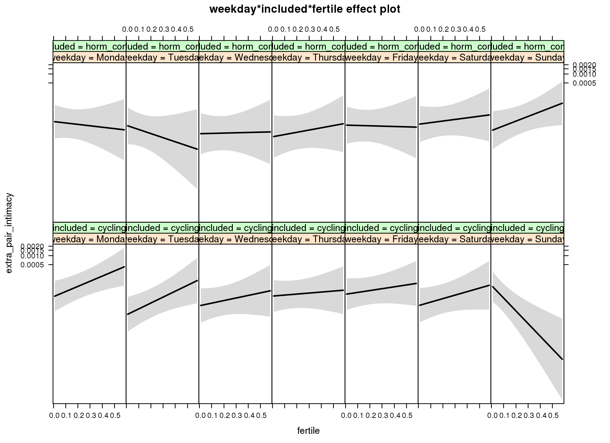
Generalized linear mixed model fit by maximum likelihood (Laplace Approximation) ['glmerMod']
 Family: binomial  ( probit )
Formula: extra_pair_intimacy ~ menstruation + fertile_mean + (1 | person) +
    weekday + included + fertile + menstruation:included + weekday:included +
    weekday:fertile + included:fertile + weekday:included:fertile
   Data: diary

     AIC      BIC   logLik deviance df.resid
    2447     2726    -1190     2379    26669

Scaled residuals:
   Min     1Q Median     3Q    Max
-2.874 -0.006 -0.004 -0.002 11.537

Random effects:
 Groups Name        Variance Std.Dev.
 person (Intercept) 4.18     2.05
Number of obs: 26703, groups:  person, 1054

Fixed effects:
                                             Estimate Std. Error z value Pr(>|z|)
(Intercept)                                  -3.57619    0.24903  -14.36  < 2e-16 ***
menstruationpre                              -0.00607    0.12054   -0.05   0.9598
menstruationyes                               0.14069    0.10900    1.29   0.1968
fertile_mean                                 -2.66144    1.17364   -2.27   0.0233 *
weekdayTuesday                               -0.40944    0.19273   -2.12   0.0336 *
weekdayWednesday                             -0.20328    0.19321   -1.05   0.2927
weekdayThursday                               0.01403    0.18091    0.08   0.9382
weekdayFriday                                 0.05453    0.18232    0.30   0.7649
weekdaySaturday                              -0.20091    0.19372   -1.04   0.2997
weekdaySunday                                 0.25442    0.17469    1.46   0.1453
includedhorm_contra                          -0.11605    0.25162   -0.46   0.6446
fertile                                       1.16175    0.44787    2.59   0.0095 **
menstruationpre:includedhorm_contra          -0.08856    0.20555   -0.43   0.6666
menstruationyes:includedhorm_contra          -0.07662    0.18442   -0.42   0.6778
weekdayTuesday:includedhorm_contra            0.32279    0.30834    1.05   0.2952
weekdayWednesday:includedhorm_contra         -0.07131    0.32348   -0.22   0.8255
weekdayThursday:includedhorm_contra          -0.35791    0.32187   -1.11   0.2662
weekdayFriday:includedhorm_contra            -0.13485    0.30409   -0.44   0.6574
weekdaySaturday:includedhorm_contra           0.13990    0.30679    0.46   0.6484
weekdaySunday:includedhorm_contra            -0.45816    0.30001   -1.53   0.1267
weekdayTuesday:fertile                        0.17128    0.67728    0.25   0.8004
weekdayWednesday:fertile                     -0.58138    0.73061   -0.80   0.4262
weekdayThursday:fertile                      -0.93493    0.68088   -1.37   0.1697
weekdayFriday:fertile                        -0.74077    0.66161   -1.12   0.2629
weekdaySaturday:fertile                      -0.37281    0.70316   -0.53   0.5960
weekdaySunday:fertile                        -4.03253    0.96082   -4.20 0.000027 ***
includedhorm_contra:fertile                  -1.48201    0.84178   -1.76   0.0783 .
weekdayTuesday:includedhorm_contra:fertile   -0.77630    1.31809   -0.59   0.5559
weekdayWednesday:includedhorm_contra:fertile  0.97163    1.26255    0.77   0.4415
weekdayThursday:includedhorm_contra:fertile   1.76167    1.19466    1.47   0.1403
weekdayFriday:includedhorm_contra:fertile     0.98219    1.19867    0.82   0.4126
weekdaySaturday:includedhorm_contra:fertile   1.05512    1.17223    0.90   0.3681
weekdaySunday:includedhorm_contra:fertile     5.41612    1.32002    4.10 0.000041 ***
---
Signif. codes:  0 '***' 0.001 '**' 0.01 '*' 0.05 '.' 0.1 ' ' 1
convergence code: 0
Model failed to converge with max|grad| = 5.05203 (tol = 0.001, component 1)
failure to converge in 10000 evaluations
M_m5: Moderation by exclusion threshold
model %>%
test_moderator("included_levels", diary, xlevels = 4)| Df | AIC | BIC | logLik | deviance | Chisq | Chi Df | Pr(>Chisq) | |
|---|---|---|---|---|---|---|---|---|
| with_main | 16 | 2400 | 2531 | -1184 | 2368 | NA | NA | NA |
| with_mod | 22 | 2412 | 2592 | -1184 | 2368 | 0.2201 | 6 | 0.9998 |
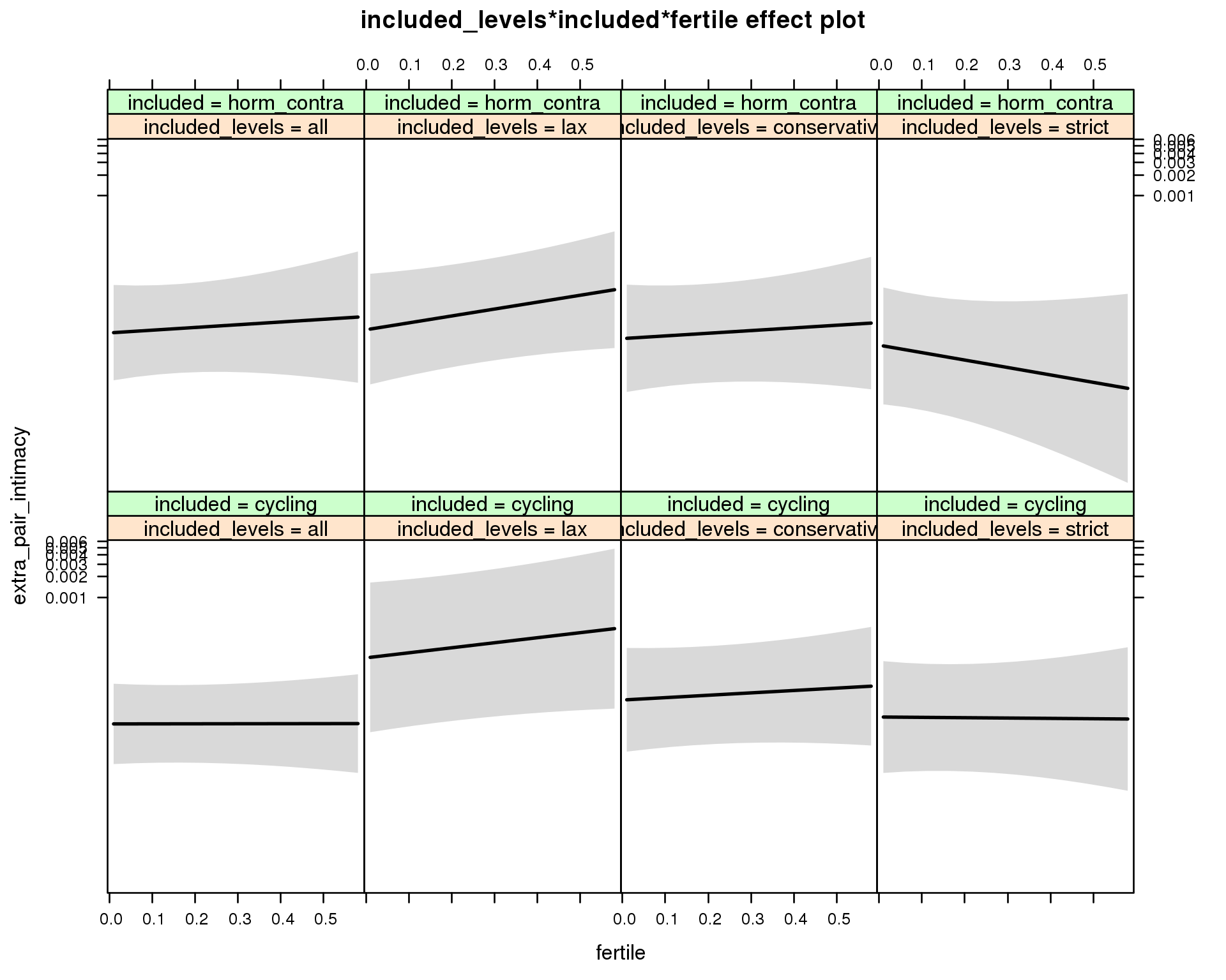
Generalized linear mixed model fit by maximum likelihood (Laplace Approximation) ['glmerMod']
 Family: binomial  ( probit )
Formula: extra_pair_intimacy ~ menstruation + fertile_mean + (1 | person) +
    included_levels + included + fertile + menstruation:included +
    included_levels:included + included_levels:fertile + included:fertile +
    included_levels:included:fertile
   Data: diary

     AIC      BIC   logLik deviance df.resid
    2412     2592    -1184     2368    26681

Scaled residuals:
   Min     1Q Median     3Q    Max
-1.917 -0.003 -0.002 -0.001 10.039

Random effects:
 Groups Name        Variance Std.Dev.
 person (Intercept) 6.85     2.62
Number of obs: 26703, groups:  person, 1054

Fixed effects:
                                                        Estimate Std. Error z value Pr(>|z|)
(Intercept)                                             -3.80135    0.27403  -13.87   <2e-16 ***
menstruationpre                                         -0.04933    0.11911   -0.41    0.679
menstruationyes                                         -0.03692    0.11410   -0.32    0.746
fertile_mean                                            -3.36367    1.53938   -2.19    0.029 *
included_levelslax                                       0.68358    0.40996    1.67    0.095 .
included_levelsconservative                              0.24723    0.30752    0.80    0.421
included_levelsstrict                                    0.07145    0.32894    0.22    0.828
includedhorm_contra                                     -0.14953    0.28766   -0.52    0.603
fertile                                                  0.00584    0.37895    0.02    0.988
menstruationpre:includedhorm_contra                      0.07469    0.20466    0.36    0.715
menstruationyes:includedhorm_contra                      0.14578    0.19066    0.76    0.444
included_levelslax:includedhorm_contra                  -0.65124    0.53799   -1.21    0.226
included_levelsconservative:includedhorm_contra         -0.30592    0.45923   -0.67    0.505
included_levelsstrict:includedhorm_contra               -0.19858    0.48751   -0.41    0.684
included_levelslax:fertile                               0.51509    0.56304    0.91    0.360
included_levelsconservative:fertile                      0.24074    0.56878    0.42    0.672
included_levelsstrict:fertile                           -0.04140    0.67940   -0.06    0.951
includedhorm_contra:fertile                              0.27626    0.71077    0.39    0.698
included_levelslax:includedhorm_contra:fertile          -0.08232    0.92380   -0.09    0.929
included_levelsconservative:includedhorm_contra:fertile -0.24668    1.00210   -0.25    0.806
included_levelsstrict:includedhorm_contra:fertile       -1.01048    1.18624   -0.85    0.394
---
Signif. codes:  0 '***' 0.001 '**' 0.01 '*' 0.05 '.' 0.1 ' ' 1
convergence code: 0
Model failed to converge with max|grad| = 2.6417 (tol = 0.001, component 1)
failure to converge in 10000 evaluations
M_m6: Moderation by cycle length
model %>%
  test_moderator("cycle_length_groups", diary, xlevels = 4)
Error: Error in pwrssUpdate(pp, resp, tol = tolPwrss, GQmat = GQmat, compDev = compDev, : Downdated VtV is not positive definite
M_m7: Moderation by certainty about menstruation parameters
model %>%
test_moderator("certainty_menstruation", diary)| Df | AIC | BIC | logLik | deviance | Chisq | Chi Df | Pr(>Chisq) | |
|---|---|---|---|---|---|---|---|---|
| with_main | 12 | 2407 | 2505 | -1191 | 2383 | NA | NA | NA |
| with_mod | 14 | 2392 | 2507 | -1182 | 2364 | 18.84 | 2 | 0.00008122 |
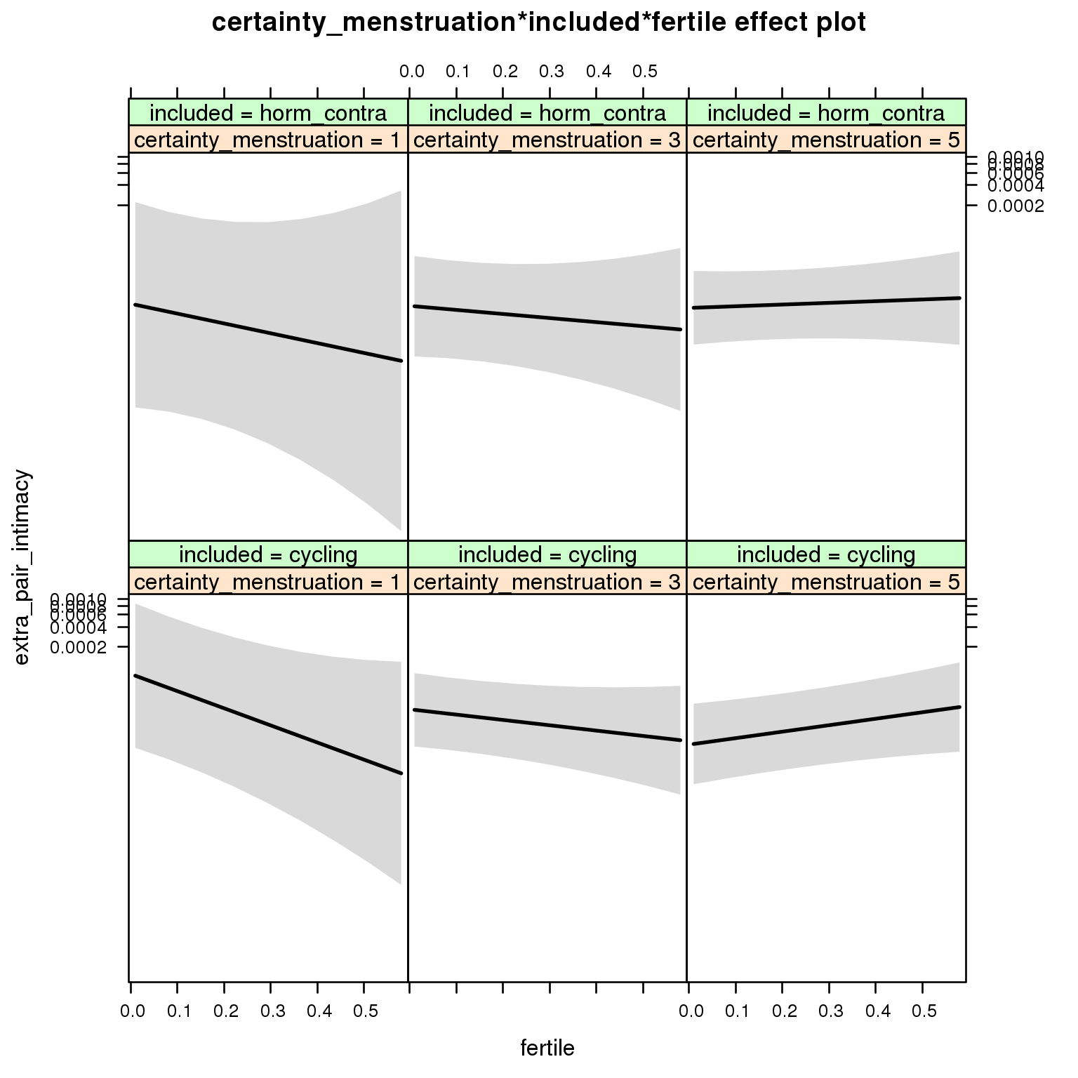
Generalized linear mixed model fit by maximum likelihood (Laplace Approximation) ['glmerMod']
 Family: binomial  ( probit )
Formula: extra_pair_intimacy ~ menstruation + fertile_mean + (1 | person) +
    certainty_menstruation + included + fertile + menstruation:included +
    certainty_menstruation:included + certainty_menstruation:fertile +
    included:fertile + certainty_menstruation:included:fertile
   Data: diary

     AIC      BIC   logLik deviance df.resid
    2392     2506    -1182     2364    26689

Scaled residuals:
   Min     1Q Median     3Q    Max
-2.126 -0.003 -0.002 -0.002  7.996

Random effects:
 Groups Name        Variance Std.Dev.
 person (Intercept) 7.32     2.71
Number of obs: 26703, groups:  person, 1054

Fixed effects:
                                                   Estimate Std. Error z value Pr(>|z|)
(Intercept)                                         -3.4721     0.4826   -7.20  6.2e-13 ***
menstruationpre                                     -0.0534     0.1217   -0.44    0.661
menstruationyes                                      0.1407     0.1109    1.27    0.205
fertile_mean                                        -0.9822     1.3538   -0.73    0.468
certainty_menstruation                              -0.1651     0.1091   -1.51    0.130
includedhorm_contra                                 -0.7793     0.7643   -1.02    0.308
fertile                                             -2.1533     1.0925   -1.97    0.049 *
menstruationpre:includedhorm_contra                 -0.1290     0.2107   -0.61    0.540
menstruationyes:includedhorm_contra                 -0.1351     0.1886   -0.72    0.474
certainty_menstruation:includedhorm_contra           0.1554     0.1778    0.87    0.382
certainty_menstruation:fertile                       0.5517     0.2460    2.24    0.025 *
includedhorm_contra:fertile                          0.9642     2.1468    0.45    0.653
certainty_menstruation:includedhorm_contra:fertile  -0.2822     0.4752   -0.59    0.553
---
Signif. codes:  0 '***' 0.001 '**' 0.01 '*' 0.05 '.' 0.1 ' ' 1
convergence code: 0
Model failed to converge with max|grad| = 2.47636 (tol = 0.001, component 1)
M_m8: Moderation by cycle regularity
model %>%
test_moderator("cycle_regularity", diary)| Df | AIC | BIC | logLik | deviance | Chisq | Chi Df | Pr(>Chisq) | |
|---|---|---|---|---|---|---|---|---|
| with_main | 14 | 2408 | 2522 | -1190 | 2380 | NA | NA | NA |
| with_mod | 18 | 2414 | 2561 | -1189 | 2378 | 1.986 | 4 | 0.7383 |
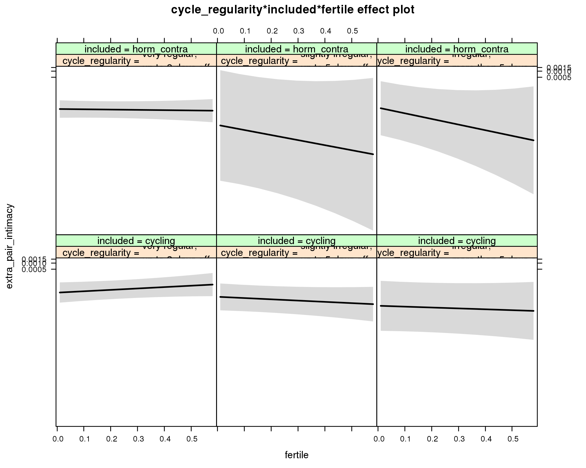
Generalized linear mixed model fit by maximum likelihood (Laplace Approximation) ['glmerMod']
 Family: binomial  ( probit )
Formula: extra_pair_intimacy ~ menstruation + fertile_mean + (1 | person) +
    cycle_regularity + included + fertile + menstruation:included +
    cycle_regularity:included + cycle_regularity:fertile + included:fertile +
    cycle_regularity:included:fertile
   Data: diary

     AIC      BIC   logLik deviance df.resid
    2414     2561    -1189     2378    26685

Scaled residuals:
   Min     1Q Median     3Q    Max
-2.038 -0.004 -0.003 -0.002  9.297

Random effects:
 Groups Name        Variance Std.Dev.
 person (Intercept) 5.33     2.31
Number of obs: 26703, groups:  person, 1054

Fixed effects:
                                                                                  Estimate Std. Error z value
(Intercept)                                                                        -3.9780     0.2740  -14.52
menstruationpre                                                                    -0.1010     0.1217   -0.83
menstruationyes                                                                     0.0364     0.1123    0.32
fertile_mean                                                                       -0.3239     1.2489   -0.26
cycle_regularityslightly irregular,\nup to 5 days off                              -0.1333     0.2463   -0.54
cycle_regularityirregular,\nmore than 5 days off                                   -0.4224     0.4148   -1.02
includedhorm_contra                                                                -0.2031     0.2082   -0.98
fertile                                                                             0.4481     0.3212    1.39
menstruationpre:includedhorm_contra                                                -0.1399     0.2076   -0.67
menstruationyes:includedhorm_contra                                                -0.2082     0.1958   -1.06
cycle_regularityslightly irregular,\nup to 5 days off:includedhorm_contra          -0.3813     0.9418   -0.40
cycle_regularityirregular,\nmore than 5 days off:includedhorm_contra                0.4653     0.6090    0.76
cycle_regularityslightly irregular,\nup to 5 days off:fertile                      -0.8572     0.4882   -1.76
cycle_regularityirregular,\nmore than 5 days off:fertile                           -0.7337     0.6344   -1.16
includedhorm_contra:fertile                                                        -0.5403     0.4540   -1.19
cycle_regularityslightly irregular,\nup to 5 days off:includedhorm_contra:fertile  -0.6787     1.8451   -0.37
cycle_regularityirregular,\nmore than 5 days off:includedhorm_contra:fertile       -0.9897     1.6223   -0.61
                                                                                  Pr(>|z|)
(Intercept)                                                                         <2e-16 ***
menstruationpre                                                                      0.407
menstruationyes                                                                      0.746
fertile_mean                                                                         0.795
cycle_regularityslightly irregular,\nup to 5 days off                                0.588
cycle_regularityirregular,\nmore than 5 days off                                     0.309
includedhorm_contra                                                                  0.329
fertile                                                                              0.163
menstruationpre:includedhorm_contra                                                  0.500
menstruationyes:includedhorm_contra                                                  0.288
cycle_regularityslightly irregular,\nup to 5 days off:includedhorm_contra            0.686
cycle_regularityirregular,\nmore than 5 days off:includedhorm_contra                 0.445
cycle_regularityslightly irregular,\nup to 5 days off:fertile                        0.079 .
cycle_regularityirregular,\nmore than 5 days off:fertile                             0.247
includedhorm_contra:fertile                                                          0.234
cycle_regularityslightly irregular,\nup to 5 days off:includedhorm_contra:fertile    0.713
cycle_regularityirregular,\nmore than 5 days off:includedhorm_contra:fertile         0.542
---
Signif. codes:  0 '***' 0.001 '**' 0.01 '*' 0.05 '.' 0.1 ' ' 1
convergence code: 0
Model failed to converge with max|grad| = 2.20935 (tol = 0.001, component 1)
M_m9: Moderation by cohabitation status
model %>%
test_moderator("cohabitation", diary)| Df | AIC | BIC | logLik | deviance | Chisq | Chi Df | Pr(>Chisq) | |
|---|---|---|---|---|---|---|---|---|
| with_main | 14 | 2394 | 2508 | -1183 | 2366 | NA | NA | NA |
| with_mod | 18 | 2397 | 2545 | -1181 | 2361 | 4.484 | 4 | 0.3444 |
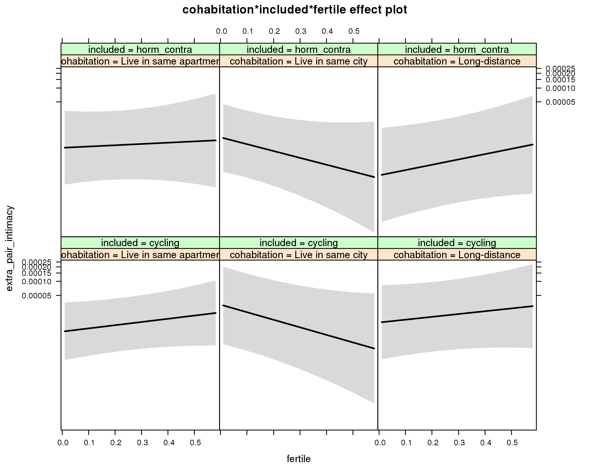
Generalized linear mixed model fit by maximum likelihood (Laplace Approximation) ['glmerMod']
 Family: binomial  ( probit )
Formula: extra_pair_intimacy ~ menstruation + fertile_mean + (1 | person) +
    cohabitation + included + fertile + menstruation:included +
    cohabitation:included + cohabitation:fertile + included:fertile +      cohabitation:included:fertile
   Data: diary

     AIC      BIC   logLik deviance df.resid
    2397     2545    -1181     2361    26685

Scaled residuals:
   Min     1Q Median     3Q    Max
-2.151 -0.004 -0.002 -0.002  8.326

Random effects:
 Groups Name        Variance Std.Dev.
 person (Intercept) 6.78     2.6
Number of obs: 26703, groups:  person, 1054

Fixed effects:
                                                          Estimate Std. Error z value Pr(>|z|)
(Intercept)                                                -3.9906     0.2789  -14.31   <2e-16 ***
menstruationpre                                            -0.1270     0.1200   -1.06    0.290
menstruationyes                                            -0.1325     0.1151   -1.15    0.250
fertile_mean                                               -1.7258     1.3371   -1.29    0.197
cohabitationLive in same city                               0.3309     0.2728    1.21    0.225
cohabitationLong-distance                                   0.1122     0.2668    0.42    0.674
includedhorm_contra                                        -0.1394     0.2814   -0.50    0.620
fertile                                                     0.3942     0.3313    1.19    0.234
menstruationpre:includedhorm_contra                         0.0269     0.2061    0.13    0.896
menstruationyes:includedhorm_contra                         0.0898     0.1948    0.46    0.645
cohabitationLive in same city:includedhorm_contra          -0.2022     0.4014   -0.50    0.614
cohabitationLong-distance:includedhorm_contra              -0.4512     0.4400   -1.03    0.305
cohabitationLive in same city:fertile                      -1.3222     0.5795   -2.28    0.023 *
cohabitationLong-distance:fertile                          -0.0483     0.4954   -0.10    0.922
includedhorm_contra:fertile                                -0.2367     0.6069   -0.39    0.696
cohabitationLive in same city:includedhorm_contra:fertile   0.3229     0.9385    0.34    0.731
cohabitationLong-distance:includedhorm_contra:fertile       0.5442     0.8285    0.66    0.511
---
Signif. codes:  0 '***' 0.001 '**' 0.01 '*' 0.05 '.' 0.1 ' ' 1
convergence code: 0
Model failed to converge with max|grad| = 2.77154 (tol = 0.001, component 1)
M_m10: Moderation by relationship status
model %>%
  test_moderator("relationship_status_clean", diary)
Error: Error in pwrssUpdate(pp, resp, tol = tolPwrss, GQmat = GQmat, compDev = compDev, : Downdated VtV is not positive definite
Does extra-pair desire predict being intimate with an extra-pair mate?
diary %>%
  group_by(person) %>%
  mutate_at(vars(extra_pair_compliments, extra_pair_flirting, extra_pair_going_out),
    funs(mean, lag), na.rm = T) %>%
  glmer(extra_pair_intimacy ~
          extra_pair_compliments_mean + extra_pair_compliments +
          extra_pair_flirting_mean + extra_pair_flirting +
          # extra_pair_going_out_mean + extra_pair_going_out_lag + extra_pair_going_out +
          (1 | person), data = ., family = binomial(link = 'probit')) %>% summary()
## Generalized linear mixed model fit by maximum likelihood (Laplace Approximation) ['glmerMod']
## Family: binomial ( probit )
## Formula: extra_pair_intimacy ~ extra_pair_compliments_mean + extra_pair_compliments +
## extra_pair_flirting_mean + extra_pair_flirting + (1 | person)
## Data: .
##
## AIC BIC logLik deviance df.resid
## 2249 2299 -1118 2237 29833
##
## Scaled residuals:
## Min 1Q Median 3Q Max
## -2.601 -0.002 -0.001 0.000 29.705
##
## Random effects:
## Groups Name Variance Std.Dev.
## person (Intercept) 5.85 2.42
## Number of obs: 29839, groups: person, 1153
##
## Fixed effects:
## Estimate Std. Error z value Pr(>|z|)
## (Intercept) -5.91191 0.00202 -2928 <2e-16 ***
## extra_pair_compliments_mean -0.25323 0.00202 -126 <2e-16 ***
## extra_pair_compliments 0.35565 0.00201 177 <2e-16 ***
## extra_pair_flirting_mean 0.39682 0.00202 197 <2e-16 ***
## extra_pair_flirting 0.28080 0.00202 139 <2e-16 ***
## ---
## Signif. codes: 0 '***' 0.001 '**' 0.01 '*' 0.05 '.' 0.1 ' ' 1
##
## Correlation of Fixed Effects:
## (Intr) extr_pr_c_ extr_pr_c extr_pr_f_
## extr_pr_cm_ -0.001
## extr_pr_cmp -0.002 -0.006
## extr_pr_fl_ -0.001 -0.002 -0.003
## extr_pr_flr -0.001 -0.003 -0.005 -0.002
## convergence code: 0
## Model failed to converge with max|grad| = 0.0347624 (tol = 0.001, component 1)Extra-pair sex
model_summaries$extra_pair_sexModel summary
Model summary
model %>%
  print_summary()
Generalized linear mixed model fit by maximum likelihood (Laplace Approximation) ['glmerMod']
Family: binomial ( probit )
Formula: extra_pair_sex ~ included * (menstruation + fertile) + fertile_mean + (1 | person)
Data: diary
AIC BIC logLik deviance df.resid
1022.5 1104.7 -501.3 1002.5 27347
Scaled residuals:
Min 1Q Median 3Q Max
-0.743 -0.002 -0.001 -0.001 8.164
Random effects:
Groups Name Variance Std.Dev.
person (Intercept) 8.65 2.94
Number of obs: 27357, groups: person, 1054
Fixed effects:
Estimate Std. Error z value Pr(>|z|)
(Intercept) -3.8913 0.3126 -12.45 <2e-16 ***
includedhorm_contra -0.5226 0.3038 -1.72 0.085 .
menstruationpre -0.0963 0.1731 -0.56 0.578
menstruationyes -0.1869 0.1777 -1.05 0.293
fertile 0.2899 0.3554 0.82 0.415
fertile_mean -3.9985 2.0256 -1.97 0.048 *
includedhorm_contra:menstruationpre 0.2450 0.3313 0.74 0.460
includedhorm_contra:menstruationyes 0.2945 0.3255 0.90 0.366
includedhorm_contra:fertile 0.6250 0.6038 1.04 0.301
---
Signif. codes: 0 '***' 0.001 '**' 0.01 '*' 0.05 '.' 0.1 ' ' 1
Correlation of Fixed Effects:
(Intr) incld_ mnstrtnp mnstrtny fertil frtl_m inclddhrm_cntr:mnstrtnp
inclddhrm_c -0.223
menstrutnpr -0.183 0.202
menstrutnys -0.149 0.163 0.320
fertile -0.166 0.274 0.430 0.303
fertile_men -0.783 -0.035 -0.016 -0.007 -0.129
inclddhrm_cntr:mnstrtnp 0.098 -0.427 -0.522 -0.167 -0.222 -0.009
inclddhrm_cntr:mnstrtny 0.080 -0.359 -0.174 -0.546 -0.164 -0.007 0.317
inclddhrm_cntr:f 0.163 -0.585 -0.252 -0.178 -0.575 -0.027 0.453
inclddhrm_cntr:mnstrtny
inclddhrm_c
menstrutnpr
menstrutnys
fertile
fertile_men
inclddhrm_cntr:mnstrtnp
inclddhrm_cntr:mnstrtny
inclddhrm_cntr:f 0.341
convergence code: 0
Model failed to converge with max|grad| = 1.07467 (tol = 0.001, component 1)
Effect size standardised by residual variance (\(\frac{b}{ SD_{residual} }\)): 0.29 [-0.41;0.99].
Marginal effect plots
model %>%
  plot_all_effects()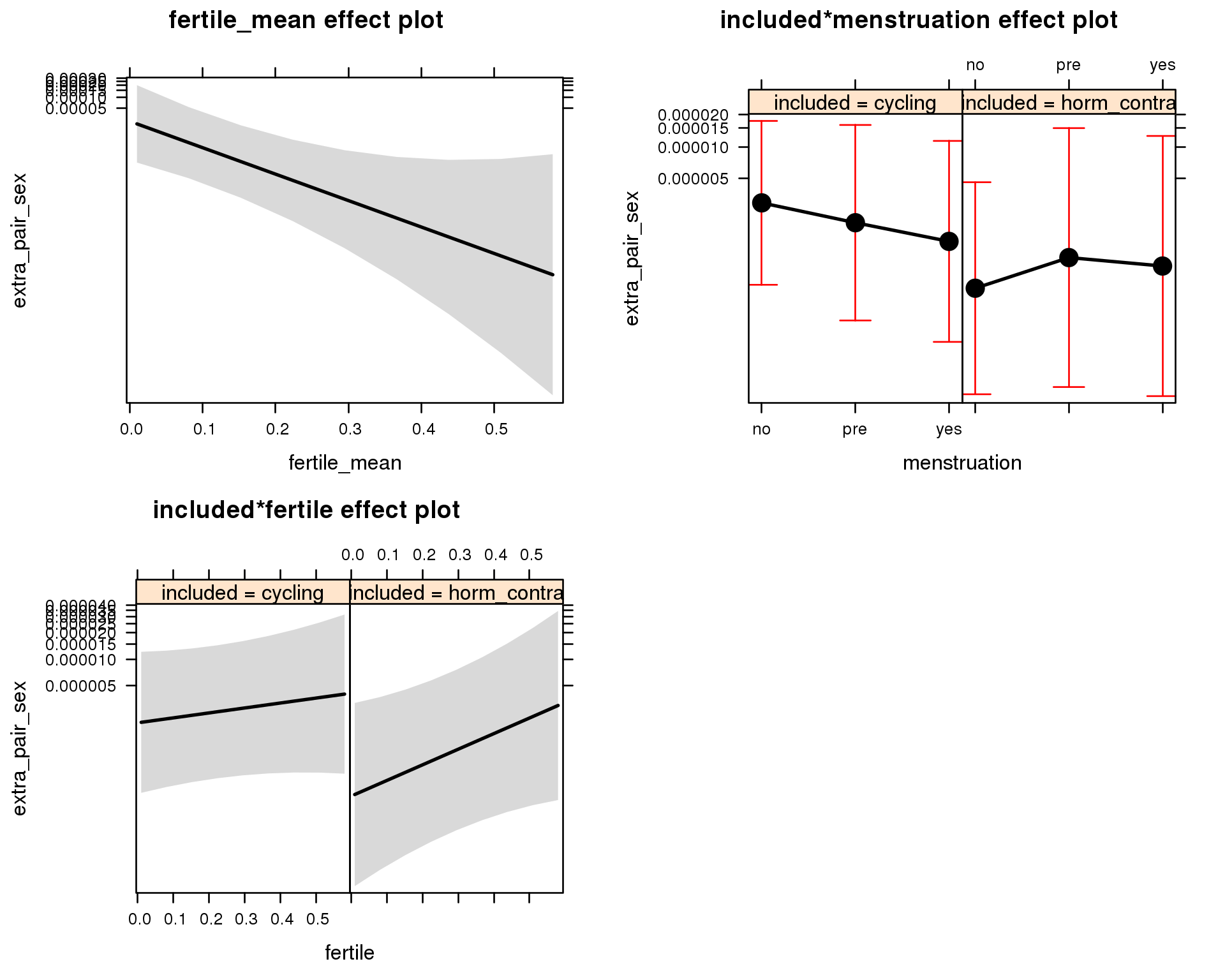
Outcome distribution
model %>%
  plot_outcome(diary) + xlab(outcome_label)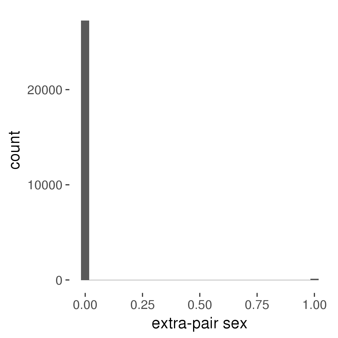
Diagnostics
model %>%
  print_diagnostics()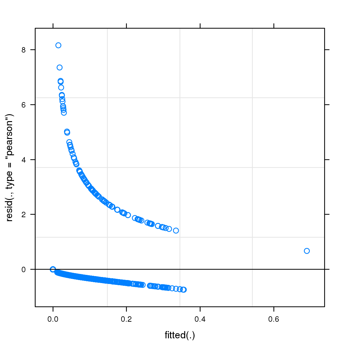
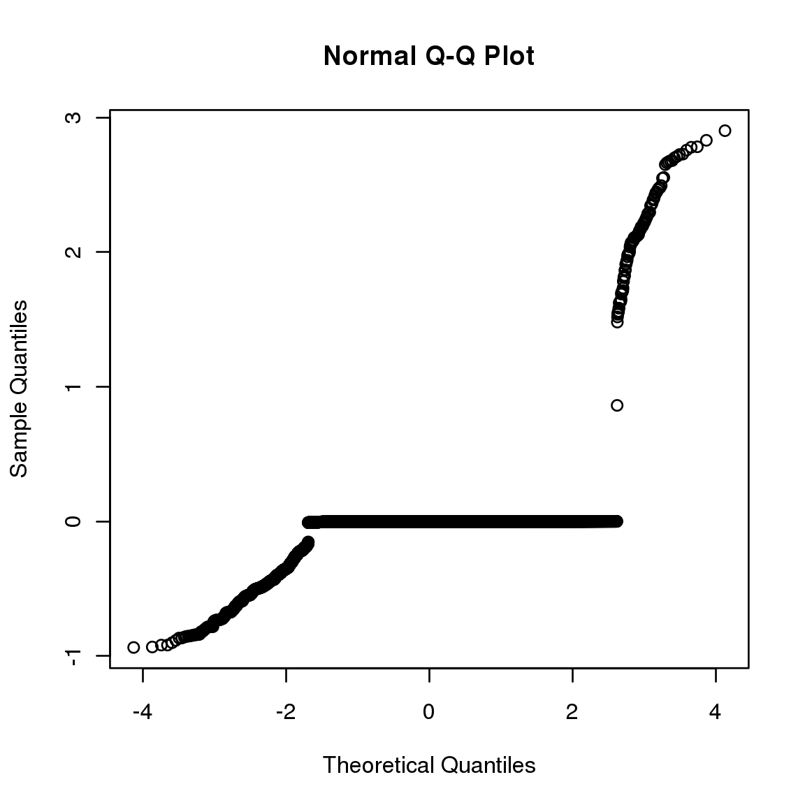
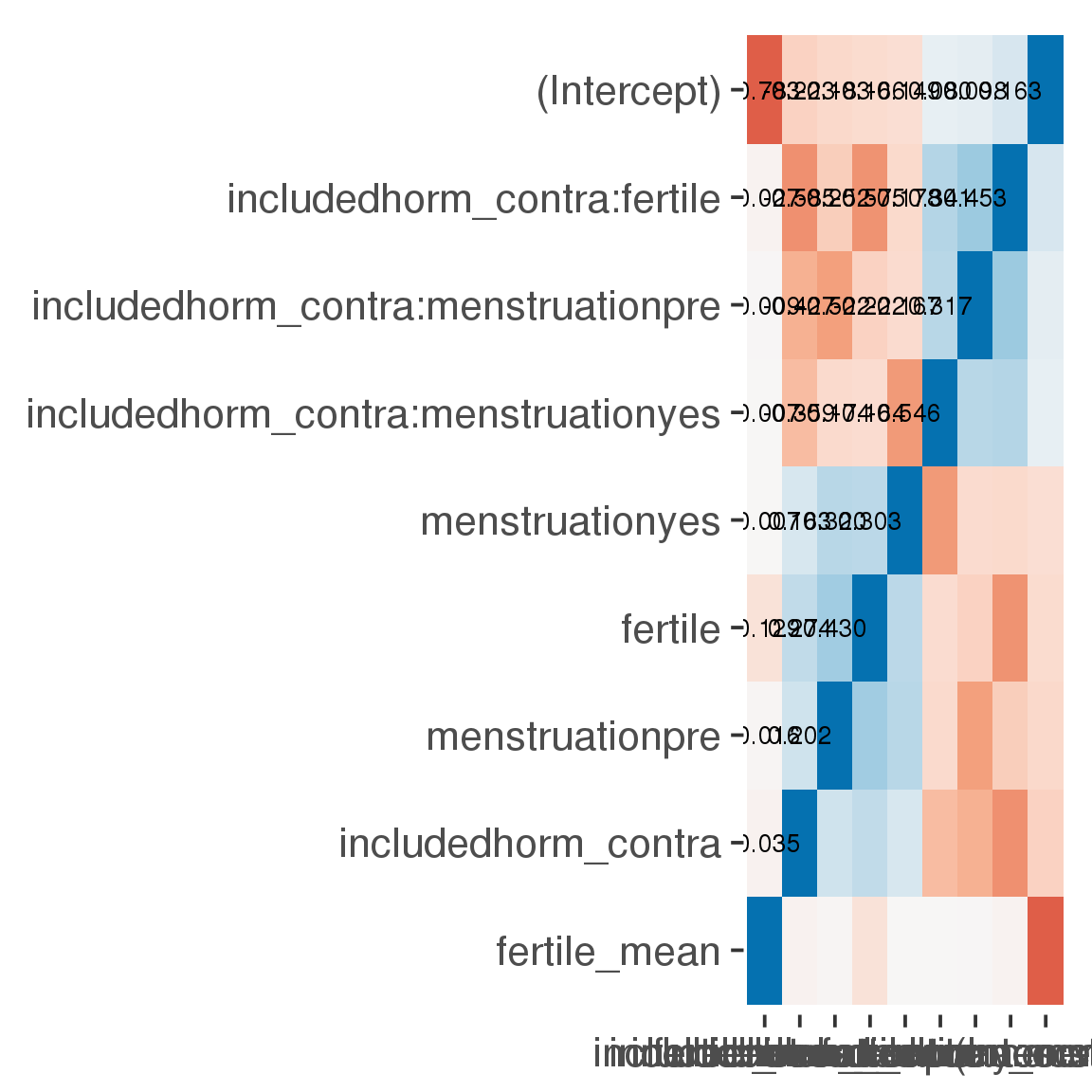
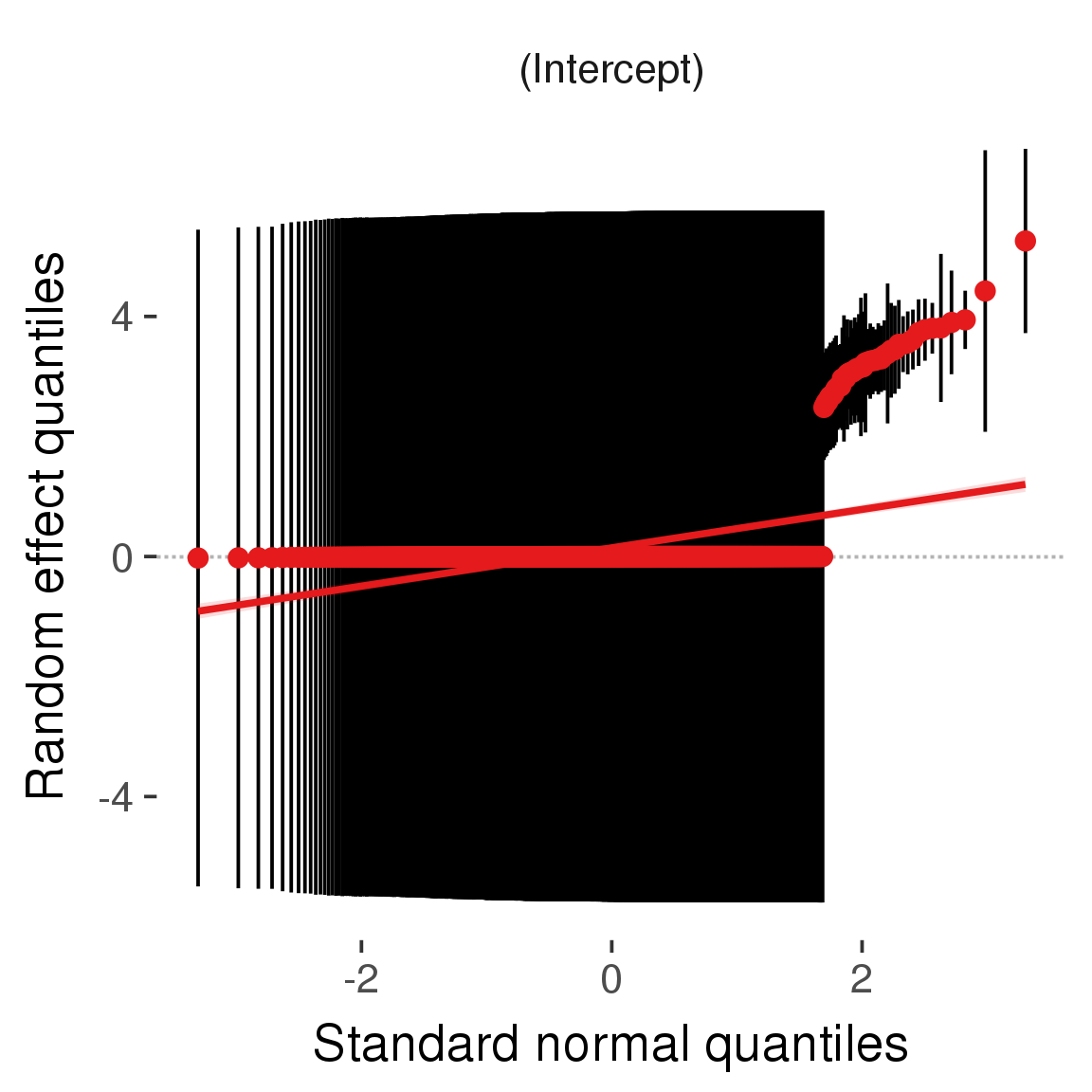
Curves
Here, we continuously plot the outcome over the course of the cycle. Because cycle lengths vary, we subset the data to cycles in a certain range. If the red curve traces the pink curve, our predictor accurately maps the relationship between fertile window probability and the outcome.
Cycle lengths from 21 to 36
Backward-counted
model %>%
  plot_curve(diary %>% filter(minimum_cycle_length_diary <= 36, minimum_cycle_length_diary > 20) %>% mutate(fertile=prc_stirn_b))
outcome = names(model@frame)[1]
outcome_label = recode(str_replace_all(str_replace_all(str_replace_all(outcome, "_", " "), " pair", "-pair"), " 1", ""),
"desirability 1" = "self-perceived desirability",
"NARQ admiration" = "narcissistic admiration",
"NARQ rivalry" = "narcissistic rivalry",
"extra-pair" = "extra-pair desire & behaviour",
"had sexual intercourse" = "sexual intercourse")
library(ggplot2)
# form a subset and run the model without the hormonal contraception and the fertility predictors
tmp = diary %>%
filter(!is.na(fertile), !is.na(included),
RCD > -1 * minimum_cycle_length_diary, RCD > -40)
new_form = update.formula(formula(model), new = . ~ . - fertile * included)
tmp$residuals = residuals(update(model, new_form, data = tmp , na.action = na.exclude))
tmp = tmp %>%
filter(!is.na(RCD), !is.na(residuals))
rcd_min = min(tmp$RCD)
tmp$real = FALSE
tmp_before = tmp
tmp_before$RCD = tmp_before$RCD + min(tmp$RCD) - 1
tmp_after = tmp
tmp_after$RCD = tmp_after$RCD - min(tmp$RCD) + 1
tmp$real = TRUE
tmp = bind_rows(tmp_before %>% filter(RCD > rcd_min - 11), tmp, tmp_after %>% filter(RCD < 11))GAM smooth on residuals
Here, we partialled out menstruation and individual random effects, then superimposed estimated probability of being in the fertile window scaled to the range of the estimated means. To address the periodicity of the cycle, we prepended and appended ten days of the timeseries to the end and the beginning of the timeseries. We then estimated the GAM and cut off the appended subsets before plotting.
tryCatch({
  trend_plot = ggplot(tmp,aes(x = RCD, y = residuals, colour = included)) +
    stat_smooth(geom = 'smooth',size = 0.8, fill = "#9ECAE1", method = 'gam', formula = y ~ s(x))
}, error = function(e){cat_message(e, "danger")})

tryCatch({
  trend_data = ggplot_build(trend_plot)$data[[1]]
}, error = function(e){cat_message(e, "danger")})

trend_data$RCD = round(trend_data$x)
trend_data = left_join(trend_data, tmp %>% select(real, RCD,fertile) %>% unique(), by = "RCD")
trend_data %>%
  filter(real == TRUE) %>%
  mutate(superimposed = ( ( (fertile - 0.01)/0.58) * (max(y)-min(y) ) ) + min(y) ) ->
  trend_data


ggplot(trend_data) +
  geom_ribbon(aes(x = x, ymin = ymin, ymax = ymax,  fill = factor(group)), alpha = 0.2) +
  geom_line(aes(x = x, y = y, colour = factor(group)), size = 0.8, stat = "identity") +
  scale_x_continuous(caption_x) +
  geom_line(aes(x = x, y = superimposed), color = "#a83fbf", size = 1, linetype = 'dashed') +
  annotate("text",x = mean(trend_data$x),  y = max(trend_data$superimposed,na.rm=T) + 0.1, label = 'superimposed fertility peak', color = "#a83fbf") +
  scale_y_continuous(outcome_label) +
  ggtitle("GAM smooth, residuals") +
  scale_color_manual("Contraception status",values = c("2"="black","1"= "red"), labels = c("2"="hormonally\ncontracepting","1"="cycling"), guide = F) +
  scale_fill_manual("Contraception status",values = c("2"="black","1"= "red"), labels = c("2"="hormonally\ncontracepting","1"="cycling"), guide = F)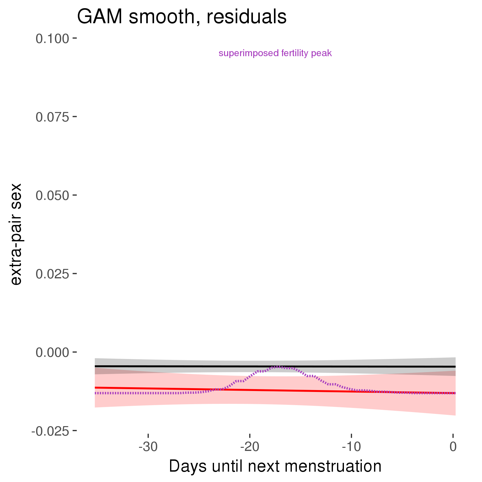
GAM smooth on raw data
As before, but without partialling anything out.
tryCatch({
  trend_plot = ggplot(tmp,aes_string(x = "RCD", y = outcome, colour = "included")) +
    stat_smooth(geom = 'smooth',size = 0.8, fill = "#9ECAE1", method = 'gam', formula = y ~ s(x))
}, error = function(e){cat_message(e, "danger")})

tryCatch({
  trend_data = ggplot_build(trend_plot)$data[[1]]
}, error = function(e){cat_message(e, "danger")})

trend_data$RCD = round(trend_data$x)
trend_data = left_join(trend_data, tmp %>% select(real, RCD,fertile) %>% unique(), by = "RCD")
trend_data %>%
  filter(real == TRUE) %>%
  mutate(superimposed = ( ( (fertile - 0.01)/0.58) * (max(y)-min(y) ) ) + min(y) ) ->
  trend_data

plot1b = ggplot(trend_data) +
  geom_ribbon(aes(x = x, ymin = ymin, ymax = ymax,  fill = factor(group)), alpha = 0.2) +
  geom_line(aes(x = x, y = y, colour = factor(group)), size = 0.8, stat = "identity") +
  scale_x_continuous(caption_x) +
  geom_line(aes(x = x, y = superimposed), color = "#a83fbf", size = 1, linetype = 'dashed') +
  annotate("text",x = mean(trend_data$x),  y = max(trend_data$superimposed,na.rm=T) + 0.1, label = 'superimposed fertility peak', color = "#a83fbf") +
  scale_y_continuous(outcome_label) +
  ggtitle("GAM smooth, raw data") +
  scale_color_manual("Contraception status",values = c("2"="black","1"= "red"), labels = c("2"="hormonally\ncontracepting","1"="cycling"), guide = F) +
  scale_fill_manual("Contraception status",values = c("2"="black","1"= "red"), labels = c("2"="hormonally\ncontracepting","1"="cycling"), guide = F)

suppressWarnings(print(plot1b))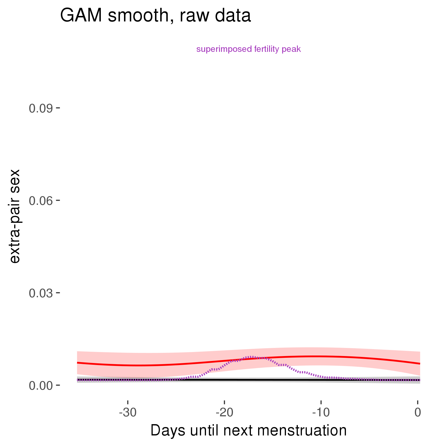
Means and standard errors over raw data
Nothing partialled out, just straight means with bootstrapped confidence intervals.
tryCatch({
  trend_plot = ggplot(tmp,aes_string(x = "RCD", y = outcome, colour = "included")) +
    geom_pointrange(size = 0.8, stat = 'summary', fun.data = "mean_cl_boot")
}, error = function(e){cat_message(e, "danger")})
tryCatch({
  trend_data = ggplot_build(trend_plot)$data[[1]]
}, error = function(e){cat_message(e, "danger")})

trend_data$RCD = round(trend_data$x)
trend_data = left_join(trend_data, tmp %>% select(real, RCD,fertile) %>% unique(), by = "RCD")
trend_data %>%
  filter(real == TRUE) %>%
  mutate(superimposed = ( ( (fertile - 0.01)/0.58) * (max(y)-min(y) ) ) + min(y) ) ->
  trend_data

plot3 = ggplot(trend_data) +
  geom_pointrange(aes(x = x, y = y, ymin = ymin,ymax = ymax, colour = factor(group)), size = 0.8, stat = "identity", alpha = 0.6, position = position_dodge(width = .5)) +
  scale_x_continuous("Days until next menstruation") +
  geom_line(aes(x= x, y = superimposed), color = "#a83fbf", size = 1, linetype = 'dashed') +
  annotate("text",x = mean(trend_data$x),  y = max(trend_data$superimposed,na.rm=T) + 0.1, label = 'superimposed fertility peak', color = "#a83fbf") +
  scale_y_continuous(outcome_label) +
  ggtitle("Means with standard errors, raw data") +
  scale_color_manual("Contraception status",values = c("2"="black","1"= "red"), labels = c("2"="hormonally\ncontracepting","1"="cycling"), guide = F) +
  scale_fill_manual("Contraception status",values = c("2"="black","1"= "red"), labels = c("2"="hormonally\ncontracepting","1"="cycling"), guide = F)
suppressWarnings(print(plot3))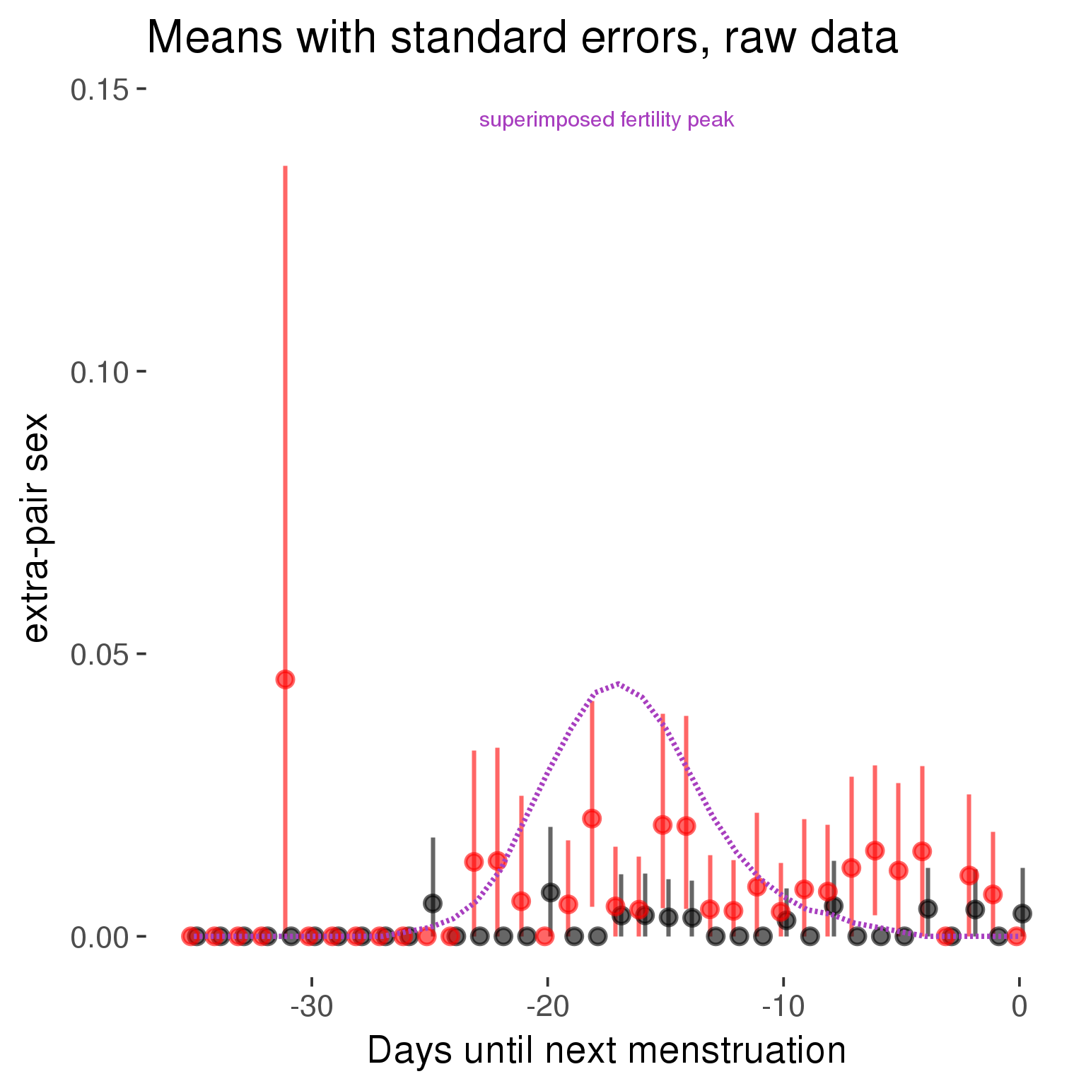
Forward-counted
model %>%
  plot_curve(diary %>% filter(minimum_cycle_length_diary <= 36, minimum_cycle_length_diary > 20) %>% mutate(RCD = FCD, fertile = prc_stirn_b_forward_counted), caption_x = "Days since last menstruation")
outcome = names(model@frame)[1]
outcome_label = recode(str_replace_all(str_replace_all(str_replace_all(outcome, "_", " "), " pair", "-pair"), " 1", ""),
"desirability 1" = "self-perceived desirability",
"NARQ admiration" = "narcissistic admiration",
"NARQ rivalry" = "narcissistic rivalry",
"extra-pair" = "extra-pair desire & behaviour",
"had sexual intercourse" = "sexual intercourse")
library(ggplot2)
# form a subset and run the model without the hormonal contraception and the fertility predictors
tmp = diary %>%
filter(!is.na(fertile), !is.na(included),
RCD > -1 * minimum_cycle_length_diary, RCD > -40)
new_form = update.formula(formula(model), new = . ~ . - fertile * included)
tmp$residuals = residuals(update(model, new_form, data = tmp , na.action = na.exclude))
tmp = tmp %>%
filter(!is.na(RCD), !is.na(residuals))
rcd_min = min(tmp$RCD)
tmp$real = FALSE
tmp_before = tmp
tmp_before$RCD = tmp_before$RCD + min(tmp$RCD) - 1
tmp_after = tmp
tmp_after$RCD = tmp_after$RCD - min(tmp$RCD) + 1
tmp$real = TRUE
tmp = bind_rows(tmp_before %>% filter(RCD > rcd_min - 11), tmp, tmp_after %>% filter(RCD < 11))GAM smooth on residuals
Here, we partialled out menstruation and individual random effects, then superimposed estimated probability of being in the fertile window scaled to the range of the estimated means. To address the periodicity of the cycle, we prepended and appended ten days of the timeseries to the end and the beginning of the timeseries. We then estimated the GAM and cut off the appended subsets before plotting.
tryCatch({
  trend_plot = ggplot(tmp,aes(x = RCD, y = residuals, colour = included)) +
    stat_smooth(geom = 'smooth',size = 0.8, fill = "#9ECAE1", method = 'gam', formula = y ~ s(x))
}, error = function(e){cat_message(e, "danger")})

tryCatch({
  trend_data = ggplot_build(trend_plot)$data[[1]]
}, error = function(e){cat_message(e, "danger")})

trend_data$RCD = round(trend_data$x)
trend_data = left_join(trend_data, tmp %>% select(real, RCD,fertile) %>% unique(), by = "RCD")
trend_data %>%
  filter(real == TRUE) %>%
  mutate(superimposed = ( ( (fertile - 0.01)/0.58) * (max(y)-min(y) ) ) + min(y) ) ->
  trend_data


ggplot(trend_data) +
  geom_ribbon(aes(x = x, ymin = ymin, ymax = ymax,  fill = factor(group)), alpha = 0.2) +
  geom_line(aes(x = x, y = y, colour = factor(group)), size = 0.8, stat = "identity") +
  scale_x_continuous(caption_x) +
  geom_line(aes(x = x, y = superimposed), color = "#a83fbf", size = 1, linetype = 'dashed') +
  annotate("text",x = mean(trend_data$x),  y = max(trend_data$superimposed,na.rm=T) + 0.1, label = 'superimposed fertility peak', color = "#a83fbf") +
  scale_y_continuous(outcome_label) +
  ggtitle("GAM smooth, residuals") +
  scale_color_manual("Contraception status",values = c("2"="black","1"= "red"), labels = c("2"="hormonally\ncontracepting","1"="cycling"), guide = F) +
  scale_fill_manual("Contraception status",values = c("2"="black","1"= "red"), labels = c("2"="hormonally\ncontracepting","1"="cycling"), guide = F)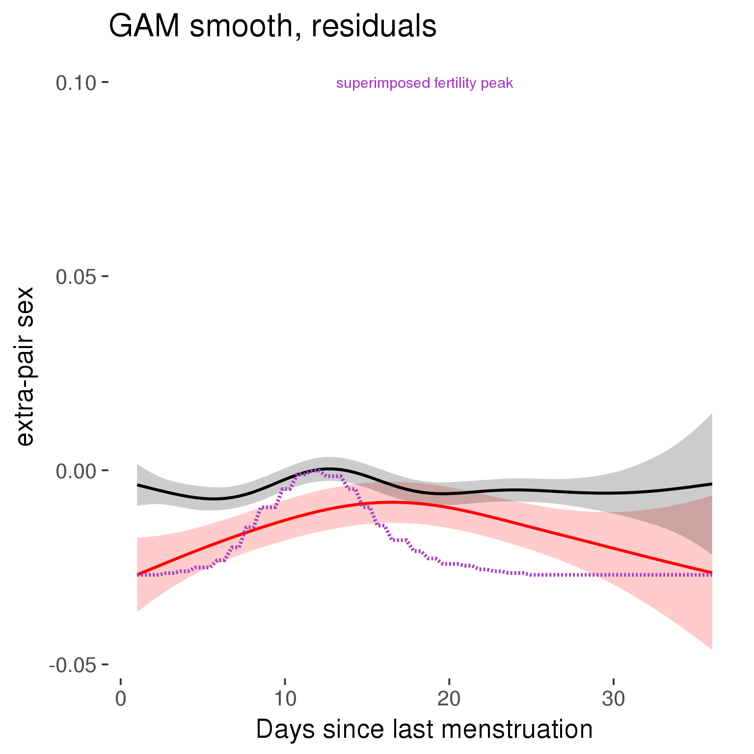
GAM smooth on raw data
As before, but without partialling anything out.
tryCatch({
  trend_plot = ggplot(tmp,aes_string(x = "RCD", y = outcome, colour = "included")) +
    stat_smooth(geom = 'smooth',size = 0.8, fill = "#9ECAE1", method = 'gam', formula = y ~ s(x))
}, error = function(e){cat_message(e, "danger")})

tryCatch({
  trend_data = ggplot_build(trend_plot)$data[[1]]
}, error = function(e){cat_message(e, "danger")})

trend_data$RCD = round(trend_data$x)
trend_data = left_join(trend_data, tmp %>% select(real, RCD,fertile) %>% unique(), by = "RCD")
trend_data %>%
  filter(real == TRUE) %>%
  mutate(superimposed = ( ( (fertile - 0.01)/0.58) * (max(y)-min(y) ) ) + min(y) ) ->
  trend_data

plot1b = ggplot(trend_data) +
  geom_ribbon(aes(x = x, ymin = ymin, ymax = ymax,  fill = factor(group)), alpha = 0.2) +
  geom_line(aes(x = x, y = y, colour = factor(group)), size = 0.8, stat = "identity") +
  scale_x_continuous(caption_x) +
  geom_line(aes(x = x, y = superimposed), color = "#a83fbf", size = 1, linetype = 'dashed') +
  annotate("text",x = mean(trend_data$x),  y = max(trend_data$superimposed,na.rm=T) + 0.1, label = 'superimposed fertility peak', color = "#a83fbf") +
  scale_y_continuous(outcome_label) +
  ggtitle("GAM smooth, raw data") +
  scale_color_manual("Contraception status",values = c("2"="black","1"= "red"), labels = c("2"="hormonally\ncontracepting","1"="cycling"), guide = F) +
  scale_fill_manual("Contraception status",values = c("2"="black","1"= "red"), labels = c("2"="hormonally\ncontracepting","1"="cycling"), guide = F)

suppressWarnings(print(plot1b))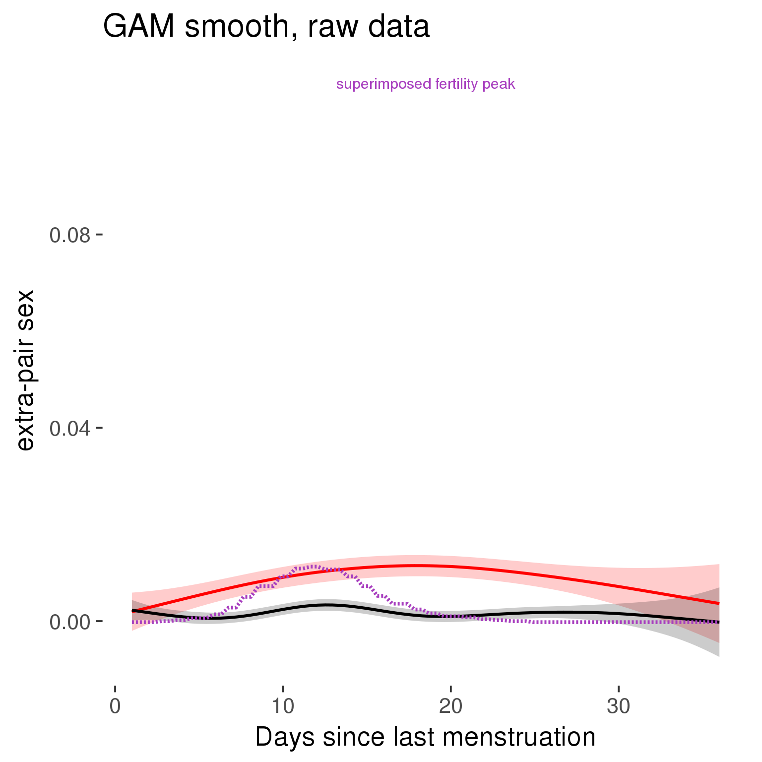
Means and standard errors over raw data
Nothing partialled out, just straight means with bootstrapped confidence intervals.
tryCatch({
  trend_plot = ggplot(tmp,aes_string(x = "RCD", y = outcome, colour = "included")) +
    geom_pointrange(size = 0.8, stat = 'summary', fun.data = "mean_cl_boot")
}, error = function(e){cat_message(e, "danger")})
tryCatch({
  trend_data = ggplot_build(trend_plot)$data[[1]]
}, error = function(e){cat_message(e, "danger")})

trend_data$RCD = round(trend_data$x)
trend_data = left_join(trend_data, tmp %>% select(real, RCD,fertile) %>% unique(), by = "RCD")
trend_data %>%
  filter(real == TRUE) %>%
  mutate(superimposed = ( ( (fertile - 0.01)/0.58) * (max(y)-min(y) ) ) + min(y) ) ->
  trend_data

plot3 = ggplot(trend_data) +
  geom_pointrange(aes(x = x, y = y, ymin = ymin,ymax = ymax, colour = factor(group)), size = 0.8, stat = "identity", alpha = 0.6, position = position_dodge(width = .5)) +
  scale_x_continuous("Days until next menstruation") +
  geom_line(aes(x= x, y = superimposed), color = "#a83fbf", size = 1, linetype = 'dashed') +
  annotate("text",x = mean(trend_data$x),  y = max(trend_data$superimposed,na.rm=T) + 0.1, label = 'superimposed fertility peak', color = "#a83fbf") +
  scale_y_continuous(outcome_label) +
  ggtitle("Means with standard errors, raw data") +
  scale_color_manual("Contraception status",values = c("2"="black","1"= "red"), labels = c("2"="hormonally\ncontracepting","1"="cycling"), guide = F) +
  scale_fill_manual("Contraception status",values = c("2"="black","1"= "red"), labels = c("2"="hormonally\ncontracepting","1"="cycling"), guide = F)
suppressWarnings(print(plot3))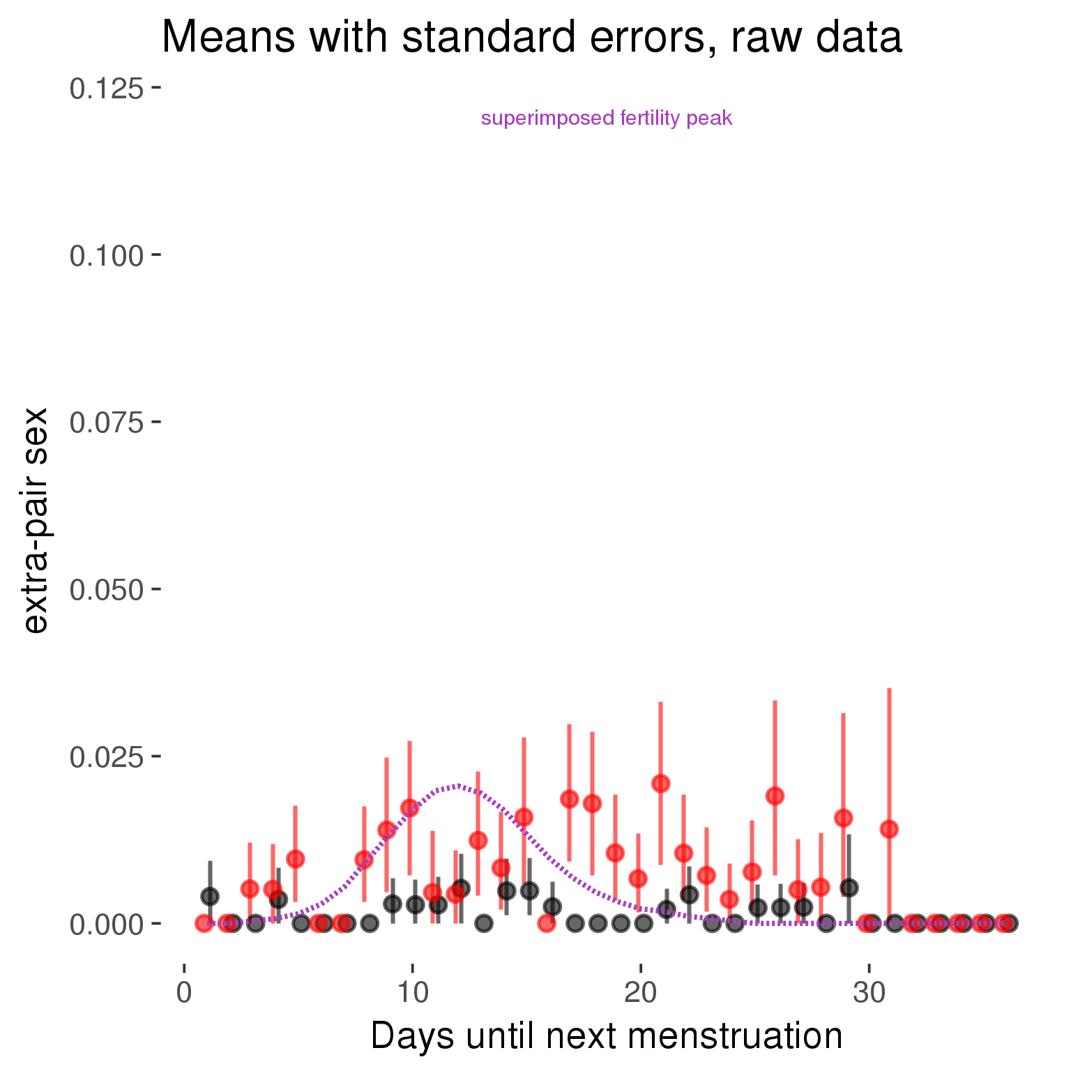
Cycle lengths from 27 to 30
Backward-counted
model %>%
  plot_curve(diary %>% filter(minimum_cycle_length_diary <= 30, minimum_cycle_length_diary >= 27) %>% mutate(fertile=prc_stirn_b))
outcome = names(model@frame)[1]
outcome_label = recode(str_replace_all(str_replace_all(str_replace_all(outcome, "_", " "), " pair", "-pair"), " 1", ""),
"desirability 1" = "self-perceived desirability",
"NARQ admiration" = "narcissistic admiration",
"NARQ rivalry" = "narcissistic rivalry",
"extra-pair" = "extra-pair desire & behaviour",
"had sexual intercourse" = "sexual intercourse")
library(ggplot2)
# form a subset and run the model without the hormonal contraception and the fertility predictors
tmp = diary %>%
filter(!is.na(fertile), !is.na(included),
RCD > -1 * minimum_cycle_length_diary, RCD > -40)
new_form = update.formula(formula(model), new = . ~ . - fertile * included)
tmp$residuals = residuals(update(model, new_form, data = tmp , na.action = na.exclude))
tmp = tmp %>%
filter(!is.na(RCD), !is.na(residuals))
rcd_min = min(tmp$RCD)
tmp$real = FALSE
tmp_before = tmp
tmp_before$RCD = tmp_before$RCD + min(tmp$RCD) - 1
tmp_after = tmp
tmp_after$RCD = tmp_after$RCD - min(tmp$RCD) + 1
tmp$real = TRUE
tmp = bind_rows(tmp_before %>% filter(RCD > rcd_min - 11), tmp, tmp_after %>% filter(RCD < 11))GAM smooth on residuals
Here, we partialled out menstruation and individual random effects, then superimposed estimated probability of being in the fertile window scaled to the range of the estimated means. To address the periodicity of the cycle, we prepended and appended ten days of the timeseries to the end and the beginning of the timeseries. We then estimated the GAM and cut off the appended subsets before plotting.
tryCatch({
  trend_plot = ggplot(tmp,aes(x = RCD, y = residuals, colour = included)) +
    stat_smooth(geom = 'smooth',size = 0.8, fill = "#9ECAE1", method = 'gam', formula = y ~ s(x))
}, error = function(e){cat_message(e, "danger")})

tryCatch({
  trend_data = ggplot_build(trend_plot)$data[[1]]
}, error = function(e){cat_message(e, "danger")})

trend_data$RCD = round(trend_data$x)
trend_data = left_join(trend_data, tmp %>% select(real, RCD,fertile) %>% unique(), by = "RCD")
trend_data %>%
  filter(real == TRUE) %>%
  mutate(superimposed = ( ( (fertile - 0.01)/0.58) * (max(y)-min(y) ) ) + min(y) ) ->
  trend_data


ggplot(trend_data) +
  geom_ribbon(aes(x = x, ymin = ymin, ymax = ymax,  fill = factor(group)), alpha = 0.2) +
  geom_line(aes(x = x, y = y, colour = factor(group)), size = 0.8, stat = "identity") +
  scale_x_continuous(caption_x) +
  geom_line(aes(x = x, y = superimposed), color = "#a83fbf", size = 1, linetype = 'dashed') +
  annotate("text",x = mean(trend_data$x),  y = max(trend_data$superimposed,na.rm=T) + 0.1, label = 'superimposed fertility peak', color = "#a83fbf") +
  scale_y_continuous(outcome_label) +
  ggtitle("GAM smooth, residuals") +
  scale_color_manual("Contraception status",values = c("2"="black","1"= "red"), labels = c("2"="hormonally\ncontracepting","1"="cycling"), guide = F) +
  scale_fill_manual("Contraception status",values = c("2"="black","1"= "red"), labels = c("2"="hormonally\ncontracepting","1"="cycling"), guide = F)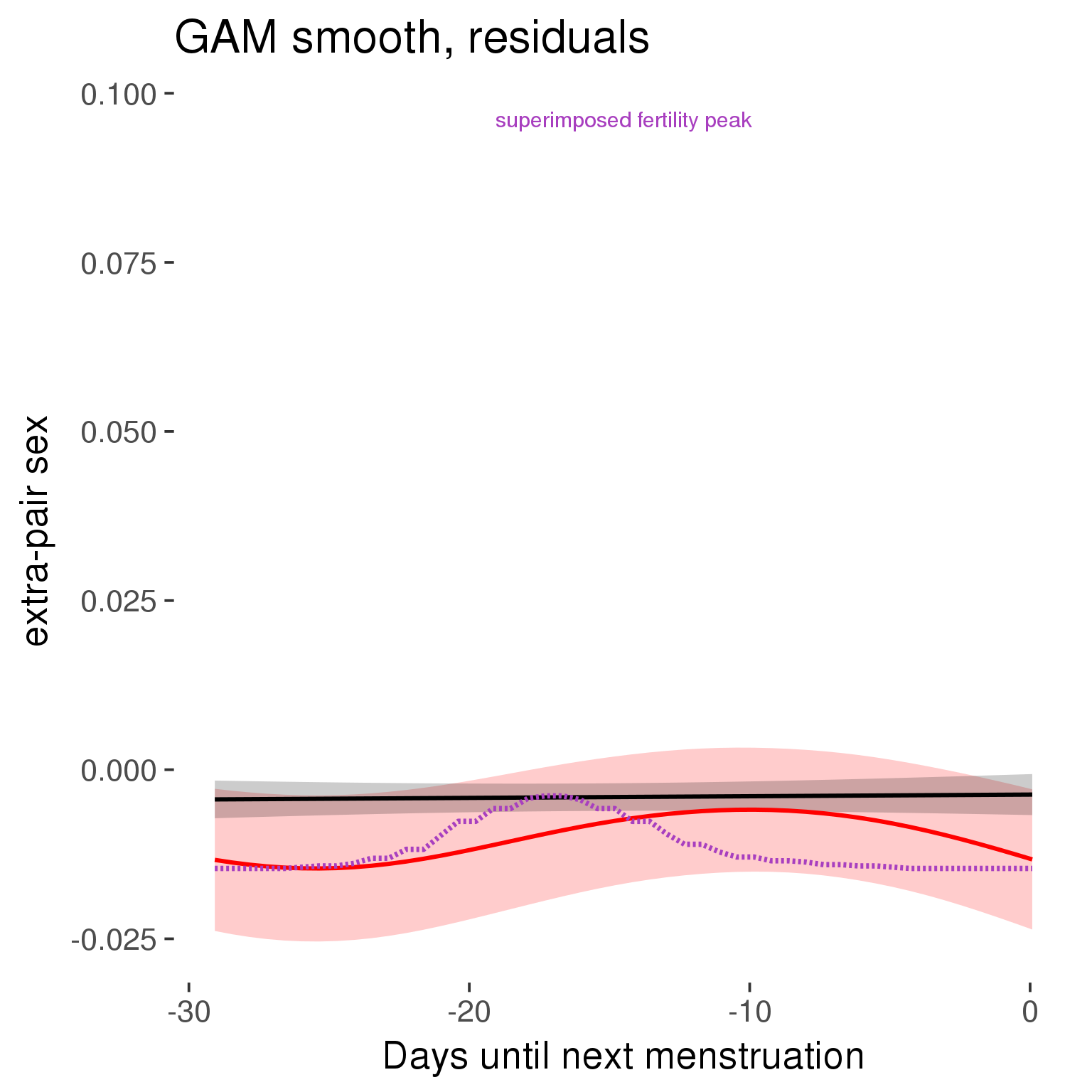
GAM smooth on raw data
As before, but without partialling anything out.
tryCatch({
  trend_plot = ggplot(tmp,aes_string(x = "RCD", y = outcome, colour = "included")) +
    stat_smooth(geom = 'smooth',size = 0.8, fill = "#9ECAE1", method = 'gam', formula = y ~ s(x))
}, error = function(e){cat_message(e, "danger")})

tryCatch({
  trend_data = ggplot_build(trend_plot)$data[[1]]
}, error = function(e){cat_message(e, "danger")})

trend_data$RCD = round(trend_data$x)
trend_data = left_join(trend_data, tmp %>% select(real, RCD,fertile) %>% unique(), by = "RCD")
trend_data %>%
  filter(real == TRUE) %>%
  mutate(superimposed = ( ( (fertile - 0.01)/0.58) * (max(y)-min(y) ) ) + min(y) ) ->
  trend_data

plot1b = ggplot(trend_data) +
  geom_ribbon(aes(x = x, ymin = ymin, ymax = ymax,  fill = factor(group)), alpha = 0.2) +
  geom_line(aes(x = x, y = y, colour = factor(group)), size = 0.8, stat = "identity") +
  scale_x_continuous(caption_x) +
  geom_line(aes(x = x, y = superimposed), color = "#a83fbf", size = 1, linetype = 'dashed') +
  annotate("text",x = mean(trend_data$x),  y = max(trend_data$superimposed,na.rm=T) + 0.1, label = 'superimposed fertility peak', color = "#a83fbf") +
  scale_y_continuous(outcome_label) +
  ggtitle("GAM smooth, raw data") +
  scale_color_manual("Contraception status",values = c("2"="black","1"= "red"), labels = c("2"="hormonally\ncontracepting","1"="cycling"), guide = F) +
  scale_fill_manual("Contraception status",values = c("2"="black","1"= "red"), labels = c("2"="hormonally\ncontracepting","1"="cycling"), guide = F)

suppressWarnings(print(plot1b))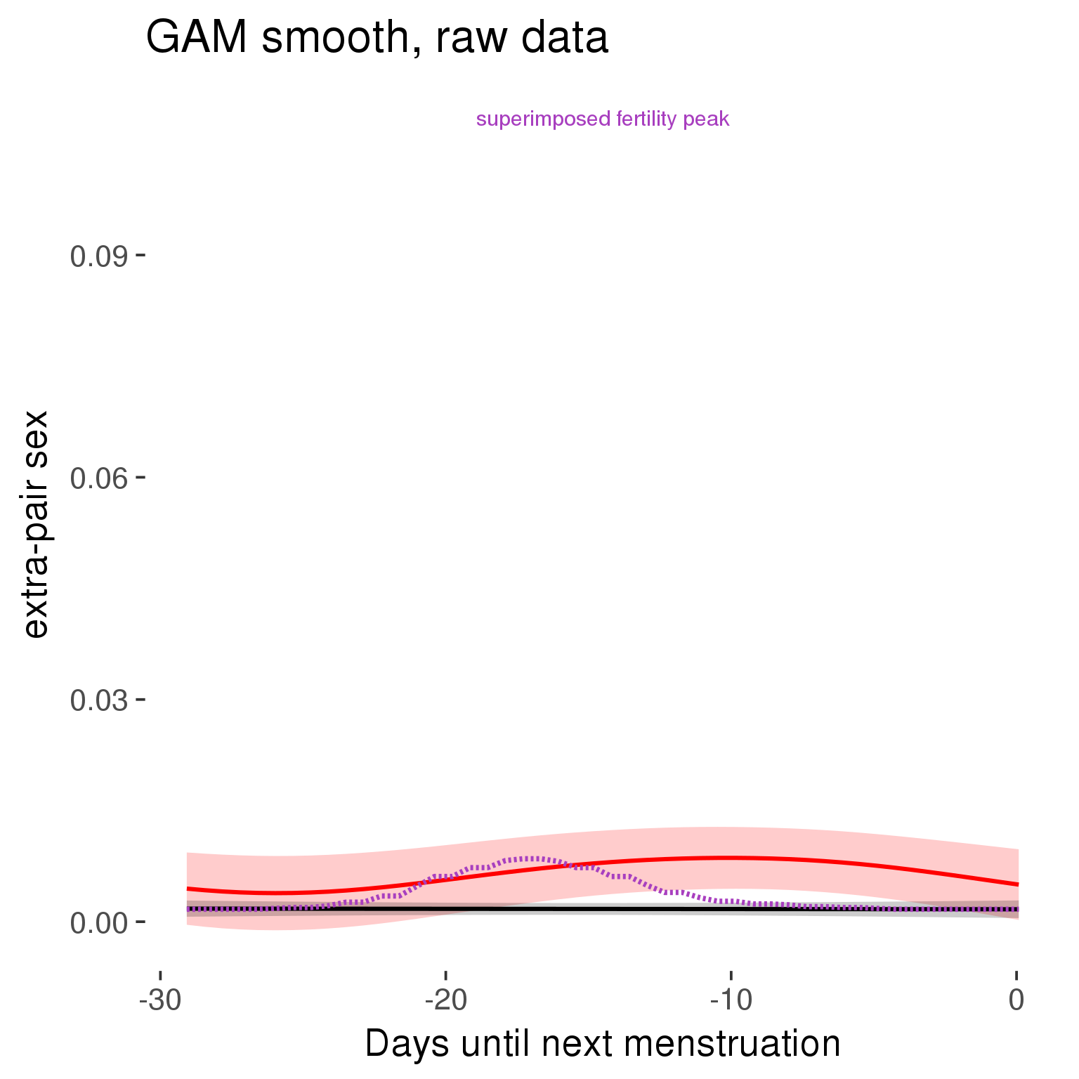
Means and standard errors over raw data
Nothing partialled out, just straight means with bootstrapped confidence intervals.
tryCatch({
  trend_plot = ggplot(tmp,aes_string(x = "RCD", y = outcome, colour = "included")) +
    geom_pointrange(size = 0.8, stat = 'summary', fun.data = "mean_cl_boot")
}, error = function(e){cat_message(e, "danger")})
tryCatch({
  trend_data = ggplot_build(trend_plot)$data[[1]]
}, error = function(e){cat_message(e, "danger")})

trend_data$RCD = round(trend_data$x)
trend_data = left_join(trend_data, tmp %>% select(real, RCD,fertile) %>% unique(), by = "RCD")
trend_data %>%
  filter(real == TRUE) %>%
  mutate(superimposed = ( ( (fertile - 0.01)/0.58) * (max(y)-min(y) ) ) + min(y) ) ->
  trend_data

plot3 = ggplot(trend_data) +
  geom_pointrange(aes(x = x, y = y, ymin = ymin,ymax = ymax, colour = factor(group)), size = 0.8, stat = "identity", alpha = 0.6, position = position_dodge(width = .5)) +
  scale_x_continuous("Days until next menstruation") +
  geom_line(aes(x= x, y = superimposed), color = "#a83fbf", size = 1, linetype = 'dashed') +
  annotate("text",x = mean(trend_data$x),  y = max(trend_data$superimposed,na.rm=T) + 0.1, label = 'superimposed fertility peak', color = "#a83fbf") +
  scale_y_continuous(outcome_label) +
  ggtitle("Means with standard errors, raw data") +
  scale_color_manual("Contraception status",values = c("2"="black","1"= "red"), labels = c("2"="hormonally\ncontracepting","1"="cycling"), guide = F) +
  scale_fill_manual("Contraception status",values = c("2"="black","1"= "red"), labels = c("2"="hormonally\ncontracepting","1"="cycling"), guide = F)
suppressWarnings(print(plot3))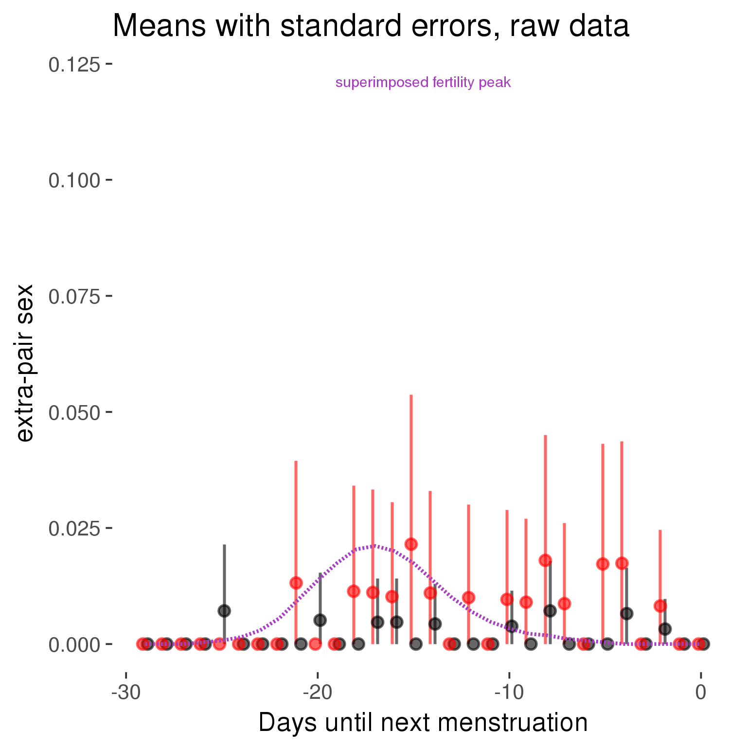
Forward-counted
model %>%
  plot_curve(diary %>% filter(minimum_cycle_length_diary <= 30, minimum_cycle_length_diary >= 27) %>% mutate(RCD = FCD, fertile = prc_stirn_b_forward_counted), caption_x = "Days since last menstruation")
outcome = names(model@frame)[1]
outcome_label = recode(str_replace_all(str_replace_all(str_replace_all(outcome, "_", " "), " pair", "-pair"), " 1", ""),
"desirability 1" = "self-perceived desirability",
"NARQ admiration" = "narcissistic admiration",
"NARQ rivalry" = "narcissistic rivalry",
"extra-pair" = "extra-pair desire & behaviour",
"had sexual intercourse" = "sexual intercourse")
library(ggplot2)
# form a subset and run the model without the hormonal contraception and the fertility predictors
tmp = diary %>%
filter(!is.na(fertile), !is.na(included),
RCD > -1 * minimum_cycle_length_diary, RCD > -40)
new_form = update.formula(formula(model), new = . ~ . - fertile * included)
tmp$residuals = residuals(update(model, new_form, data = tmp , na.action = na.exclude))
tmp = tmp %>%
filter(!is.na(RCD), !is.na(residuals))
rcd_min = min(tmp$RCD)
tmp$real = FALSE
tmp_before = tmp
tmp_before$RCD = tmp_before$RCD + min(tmp$RCD) - 1
tmp_after = tmp
tmp_after$RCD = tmp_after$RCD - min(tmp$RCD) + 1
tmp$real = TRUE
tmp = bind_rows(tmp_before %>% filter(RCD > rcd_min - 11), tmp, tmp_after %>% filter(RCD < 11))GAM smooth on residuals
Here, we partialled out menstruation and individual random effects, then superimposed estimated probability of being in the fertile window scaled to the range of the estimated means. To address the periodicity of the cycle, we prepended and appended ten days of the timeseries to the end and the beginning of the timeseries. We then estimated the GAM and cut off the appended subsets before plotting.
tryCatch({
  trend_plot = ggplot(tmp,aes(x = RCD, y = residuals, colour = included)) +
    stat_smooth(geom = 'smooth',size = 0.8, fill = "#9ECAE1", method = 'gam', formula = y ~ s(x))
}, error = function(e){cat_message(e, "danger")})

tryCatch({
  trend_data = ggplot_build(trend_plot)$data[[1]]
}, error = function(e){cat_message(e, "danger")})

trend_data$RCD = round(trend_data$x)
trend_data = left_join(trend_data, tmp %>% select(real, RCD,fertile) %>% unique(), by = "RCD")
trend_data %>%
  filter(real == TRUE) %>%
  mutate(superimposed = ( ( (fertile - 0.01)/0.58) * (max(y)-min(y) ) ) + min(y) ) ->
  trend_data


ggplot(trend_data) +
  geom_ribbon(aes(x = x, ymin = ymin, ymax = ymax,  fill = factor(group)), alpha = 0.2) +
  geom_line(aes(x = x, y = y, colour = factor(group)), size = 0.8, stat = "identity") +
  scale_x_continuous(caption_x) +
  geom_line(aes(x = x, y = superimposed), color = "#a83fbf", size = 1, linetype = 'dashed') +
  annotate("text",x = mean(trend_data$x),  y = max(trend_data$superimposed,na.rm=T) + 0.1, label = 'superimposed fertility peak', color = "#a83fbf") +
  scale_y_continuous(outcome_label) +
  ggtitle("GAM smooth, residuals") +
  scale_color_manual("Contraception status",values = c("2"="black","1"= "red"), labels = c("2"="hormonally\ncontracepting","1"="cycling"), guide = F) +
  scale_fill_manual("Contraception status",values = c("2"="black","1"= "red"), labels = c("2"="hormonally\ncontracepting","1"="cycling"), guide = F)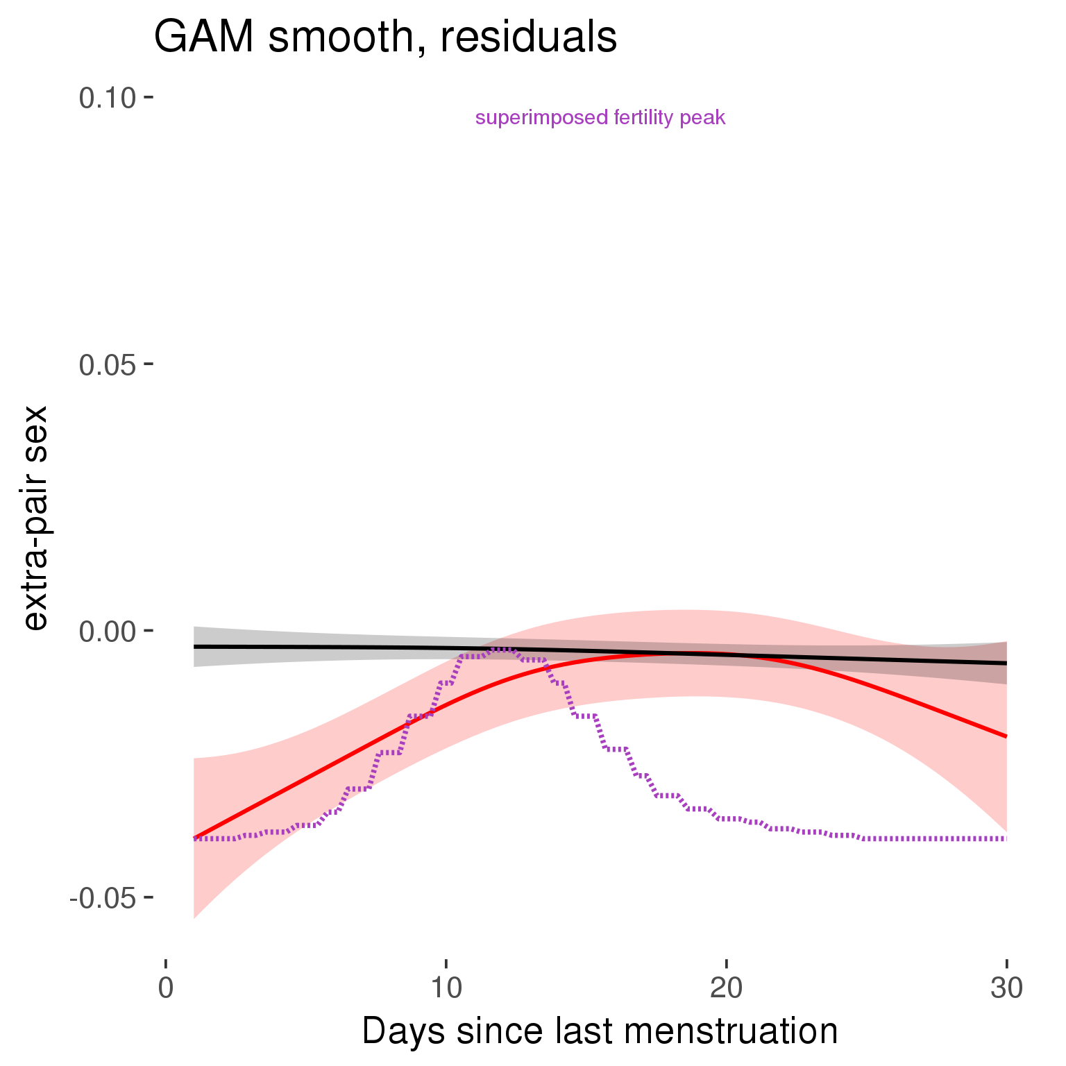
GAM smooth on raw data
As before, but without partialling anything out.
tryCatch({
  trend_plot = ggplot(tmp,aes_string(x = "RCD", y = outcome, colour = "included")) +
    stat_smooth(geom = 'smooth',size = 0.8, fill = "#9ECAE1", method = 'gam', formula = y ~ s(x))
}, error = function(e){cat_message(e, "danger")})

tryCatch({
  trend_data = ggplot_build(trend_plot)$data[[1]]
}, error = function(e){cat_message(e, "danger")})

trend_data$RCD = round(trend_data$x)
trend_data = left_join(trend_data, tmp %>% select(real, RCD,fertile) %>% unique(), by = "RCD")
trend_data %>%
  filter(real == TRUE) %>%
  mutate(superimposed = ( ( (fertile - 0.01)/0.58) * (max(y)-min(y) ) ) + min(y) ) ->
  trend_data

plot1b = ggplot(trend_data) +
  geom_ribbon(aes(x = x, ymin = ymin, ymax = ymax,  fill = factor(group)), alpha = 0.2) +
  geom_line(aes(x = x, y = y, colour = factor(group)), size = 0.8, stat = "identity") +
  scale_x_continuous(caption_x) +
  geom_line(aes(x = x, y = superimposed), color = "#a83fbf", size = 1, linetype = 'dashed') +
  annotate("text",x = mean(trend_data$x),  y = max(trend_data$superimposed,na.rm=T) + 0.1, label = 'superimposed fertility peak', color = "#a83fbf") +
  scale_y_continuous(outcome_label) +
  ggtitle("GAM smooth, raw data") +
  scale_color_manual("Contraception status",values = c("2"="black","1"= "red"), labels = c("2"="hormonally\ncontracepting","1"="cycling"), guide = F) +
  scale_fill_manual("Contraception status",values = c("2"="black","1"= "red"), labels = c("2"="hormonally\ncontracepting","1"="cycling"), guide = F)

suppressWarnings(print(plot1b))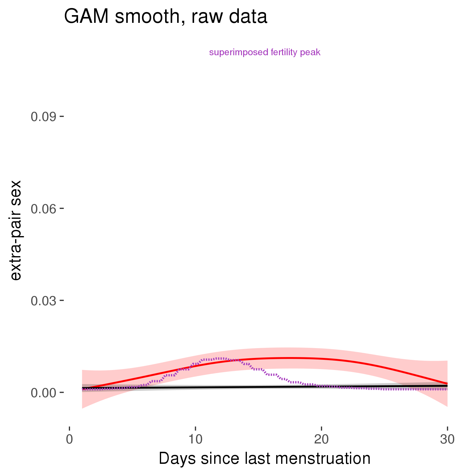
Means and standard errors over raw data
Nothing partialled out, just straight means with bootstrapped confidence intervals.
tryCatch({
  trend_plot = ggplot(tmp,aes_string(x = "RCD", y = outcome, colour = "included")) +
    geom_pointrange(size = 0.8, stat = 'summary', fun.data = "mean_cl_boot")
}, error = function(e){cat_message(e, "danger")})
tryCatch({
  trend_data = ggplot_build(trend_plot)$data[[1]]
}, error = function(e){cat_message(e, "danger")})

trend_data$RCD = round(trend_data$x)
trend_data = left_join(trend_data, tmp %>% select(real, RCD,fertile) %>% unique(), by = "RCD")
trend_data %>%
  filter(real == TRUE) %>%
  mutate(superimposed = ( ( (fertile - 0.01)/0.58) * (max(y)-min(y) ) ) + min(y) ) ->
  trend_data

plot3 = ggplot(trend_data) +
  geom_pointrange(aes(x = x, y = y, ymin = ymin,ymax = ymax, colour = factor(group)), size = 0.8, stat = "identity", alpha = 0.6, position = position_dodge(width = .5)) +
  scale_x_continuous("Days until next menstruation") +
  geom_line(aes(x= x, y = superimposed), color = "#a83fbf", size = 1, linetype = 'dashed') +
  annotate("text",x = mean(trend_data$x),  y = max(trend_data$superimposed,na.rm=T) + 0.1, label = 'superimposed fertility peak', color = "#a83fbf") +
  scale_y_continuous(outcome_label) +
  ggtitle("Means with standard errors, raw data") +
  scale_color_manual("Contraception status",values = c("2"="black","1"= "red"), labels = c("2"="hormonally\ncontracepting","1"="cycling"), guide = F) +
  scale_fill_manual("Contraception status",values = c("2"="black","1"= "red"), labels = c("2"="hormonally\ncontracepting","1"="cycling"), guide = F)
suppressWarnings(print(plot3))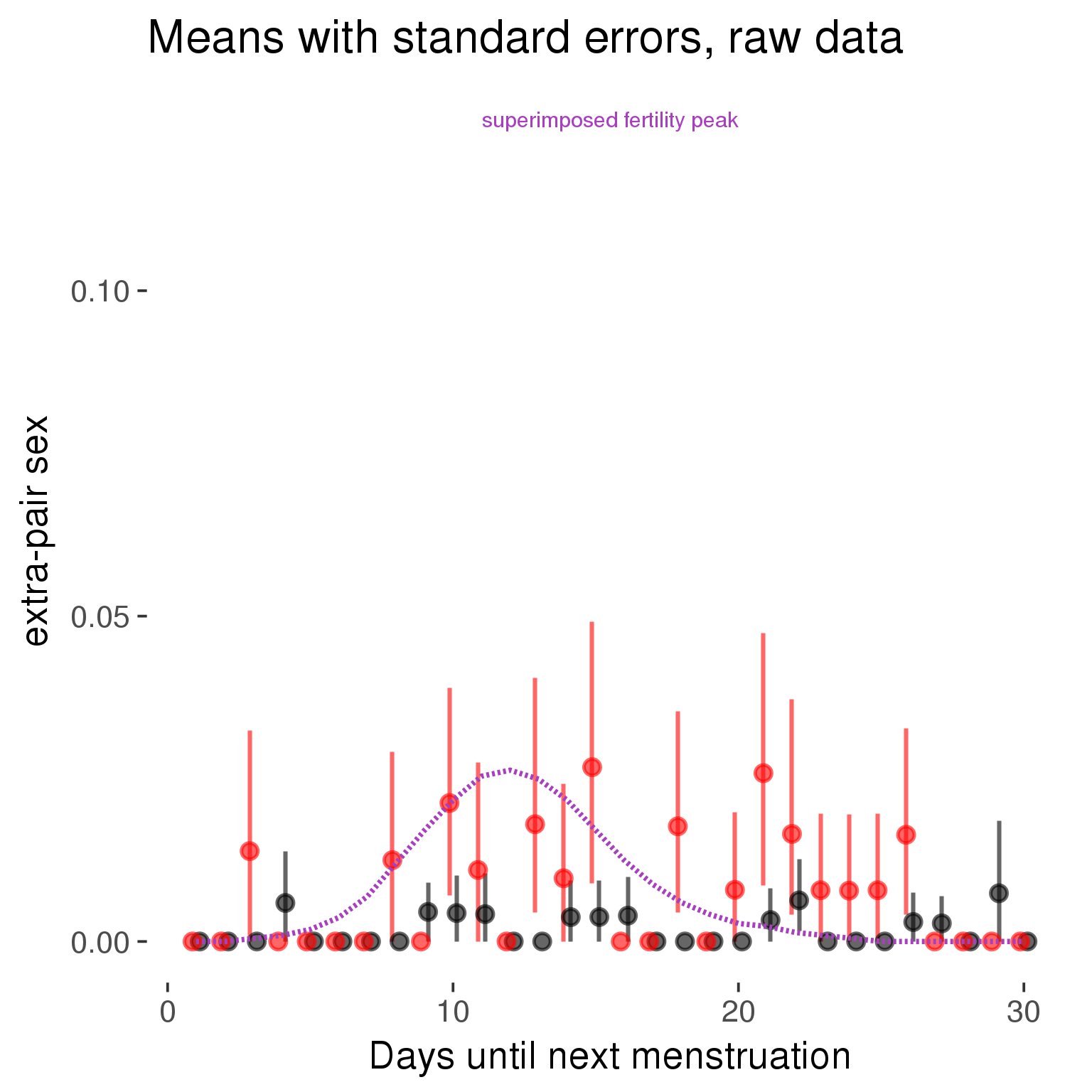
Robustness checks
M_r1: Random slopes for conception risk and menstruation
tryCatch({
# refit model with random effects for fertile and menstruation dummies
with_ind_diff = update(model, formula = . ~ . - (1| person) + (1 + fertile + menstruation | person))

# pull the random effects, format as tibble
rand = coef(with_ind_diff)$person %>%
  tibble::rownames_to_column("person") %>%
  mutate(person = as.numeric(person))

# pull the fixed effects
fixd = data.frame(fixef(with_ind_diff)) %>%
  tibble::rownames_to_column("effect")
names(fixd) = c("effect", "pop_effect_size")

# pull apart the coefficients so that we can account for the fact that the random effect variation implicitly includes HC explaining the mean population-level effect of fertile/menstruation dummies among HC users
fixd = fixd %>%
  separate(effect, c("included", "effect"), sep = ":", fill = "left") %>%
  mutate(included = if_else(is.na(included), "cycling", str_replace(included, "included", "")))
fixd[2,c("included", "effect")] = c("horm_contra", "(Intercept)")


rand = rand %>%
  # merge diary data on the random effects, so that we know who is a HC users and who isn't
  inner_join(diary %>% select(person, included) %>% unique(), by = 'person') %>%
  # gather into long format, to have the dataset by predictor
  gather(effect, value, -person, -included) %>%
  inner_join(fixd, by = c('effect', 'included')) %>%
  # pull the fixed effects
  mutate(
    # only for those who are HC users, add the moderated population effect size for this effect (the random effects have the reference category mean)
    value = if_else(included == "horm_contra", value + pop_effect_size, value),
    effect = recode(effect, "includedhorm_contra" = "HC user",
                   "includedhorm_contra:fertile" = "HC user x fertile",
                   "includedhorm_contra:menstruationpre" = "HC user x premens.",
                   "includedhorm_contra:menstruationyes" = "HC user x mens.",
                   "menstruationyes" = "mens.",
                   "menstruationpre" = "premens.")) %>%
  group_by(included, effect) %>%
  # filter out predictors that aren't modelled as varying/random
  filter(sd(value) > 0)

# plot dot plot of random effects
print(
ggplot(rand, aes(x = included, y = value, color = included, fill = included)) +
  facet_wrap( ~ effect, scales = "free") +
  # geom_violin(alpha = 0.4, size = 0) +
  geom_dotplot(binaxis='y', dotsize = 0.1, method = "histodot") +
# geom_jitter(alpha = 0.05) +
  coord_flip() +
  geom_pointrange(stat = 'summary', fun.data = 'mean_sdl', color = 'darkred', size = 1.2) +
  scale_color_manual("Contraception status", values = c("horm_contra"="black","cycling"= "red"), labels = c("horm_contra"="hormonally\ncontracepting","cycling"="cycling"), guide = F) +
  scale_fill_manual("Contraception status", values = c("horm_contra"="black","cycling"= "red"), labels = c("horm_contra"="hormonally\ncontracepting","1"="cycling"), guide = F) +
  ggtitle("M_r1: allowing participant-varying slopes", subtitle = "for the conception risk measure and the menstruation dummies") +
  scale_x_discrete("Hormonal contraception", breaks = c("horm_contra", "cycling"), labels = c("yes", "no")) +
  scale_y_continuous("Random effect size distribution"))

print_summary(with_ind_diff)
cat(pander(anova(model, with_ind_diff)))
}, error = function(e){
  with_ind_diff = model
  cat_message(e, "danger")
})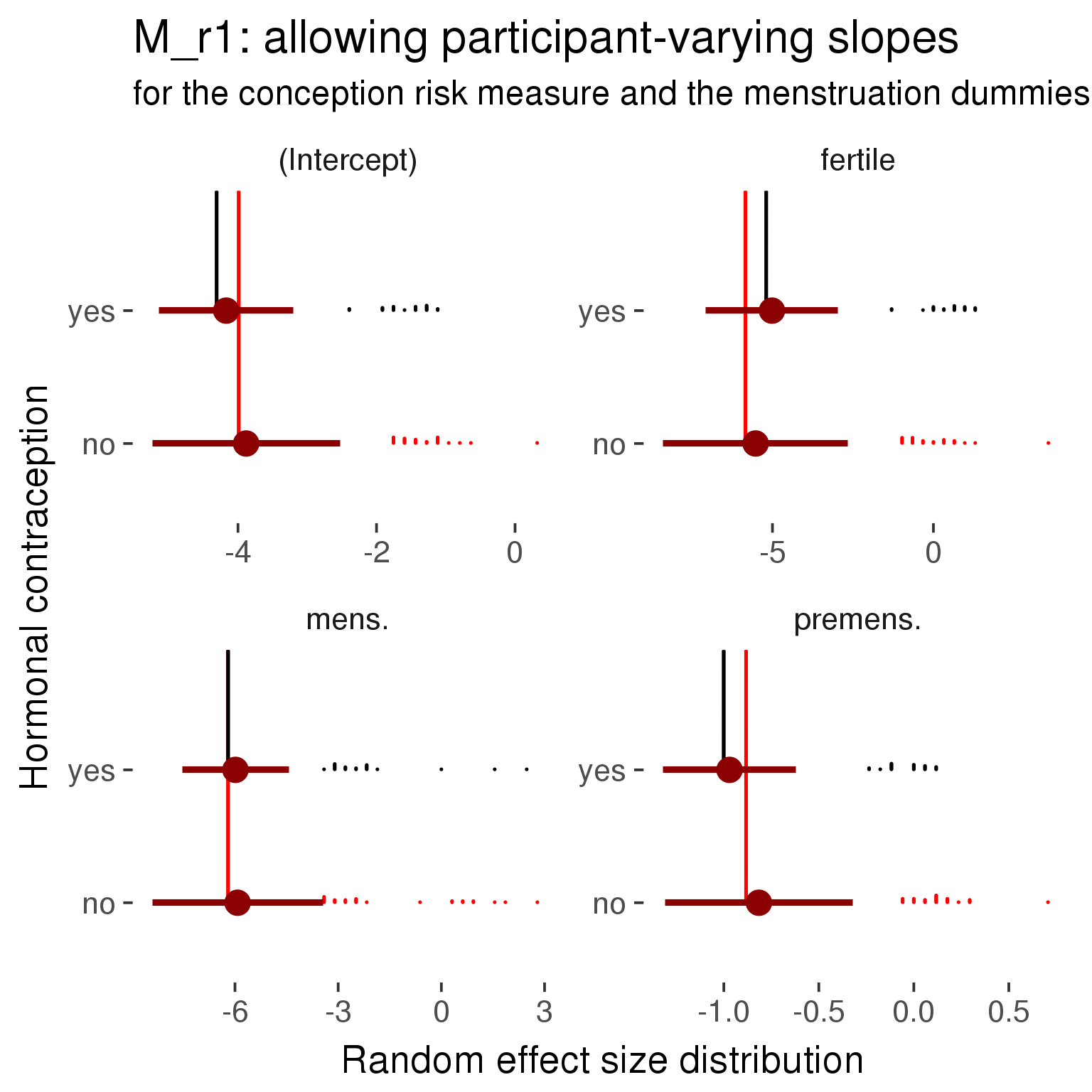
Generalized linear mixed model fit by maximum likelihood (Laplace Approximation) ['glmerMod']
 Family: binomial  ( probit )
Formula: extra_pair_sex ~ included + menstruation + fertile + fertile_mean +
    (1 + fertile + menstruation | person) + included:menstruation +      included:fertile
   Data: diary

     AIC      BIC   logLik deviance df.resid
  1041.6   1197.7   -501.8   1003.6    27338

Scaled residuals:
   Min     1Q Median     3Q    Max
-1.310 -0.001  0.000  0.000  6.419

Random effects:
 Groups Name            Variance Std.Dev. Corr
 person (Intercept)      7.678   2.771
        fertile         34.732   5.893    1.00
        menstruationpre  0.991   0.995    1.00 0.99
        menstruationyes 30.650   5.536    0.63 0.61 0.67
Number of obs: 27357, groups:  person, 1054

Fixed effects:
                                    Estimate Std. Error z value   Pr(>|z|)
(Intercept)                          -4.0537     0.8873   -4.57 0.00000491 ***
includedhorm_contra                  -0.2045     0.7850   -0.26    0.79450
menstruationpre                      -0.8779     0.2595   -3.38    0.00072 ***
menstruationyes                      -6.2157     1.4931   -4.16 0.00003143 ***
fertile                              -5.8865     1.1700   -5.03 0.00000049 ***
fertile_mean                         -0.2904     4.8992   -0.06    0.95273
includedhorm_contra:menstruationpre  -0.1242     0.4559   -0.27    0.78526
includedhorm_contra:menstruationyes   0.0965     2.8686    0.03    0.97317
includedhorm_contra:fertile           0.6839     1.8038    0.38    0.70459
---
Signif. codes:  0 '***' 0.001 '**' 0.01 '*' 0.05 '.' 0.1 ' ' 1

Correlation of Fixed Effects:
                        (Intr) incld_ mnstrtnp mnstrtny fertil frtl_m inclddhrm_cntr:mnstrtnp
inclddhrm_c             -0.329
menstrutnpr              0.326 -0.382
menstrutnys              0.233 -0.258  0.357
fertile                  0.475 -0.549  0.782    0.392
fertile_men             -0.813 -0.066  0.014   -0.006    0.013
inclddhrm_cntr:mnstrtnp -0.215  0.469 -0.569   -0.204   -0.445  0.028
inclddhrm_cntr:mnstrtny -0.073  0.300 -0.187   -0.520   -0.205 -0.057  0.242
inclddhrm_cntr:f        -0.391  0.791 -0.506   -0.255   -0.647  0.094  0.696
                        inclddhrm_cntr:mnstrtny
inclddhrm_c
menstrutnpr
menstrutnys
fertile
fertile_men
inclddhrm_cntr:mnstrtnp
inclddhrm_cntr:mnstrtny
inclddhrm_cntr:f         0.287
convergence code: 0
unable to evaluate scaled gradient
Model failed to converge: degenerate  Hessian with 4 negative eigenvalues
failure to converge in 10000 evaluations
| Df | AIC | BIC | logLik | deviance | Chisq | Chi Df | Pr(>Chisq) | |
|---|---|---|---|---|---|---|---|---|
| model | 10 | 1023 | 1105 | -501.3 | 1003 | NA | NA | NA |
| with_ind_diff | 19 | 1042 | 1198 | -501.8 | 1004 | 0 | 9 | 1 |
robustness_check_ovu_shift(model, diary)Error: Error in pwrssUpdate(pp, resp, tol = tolPwrss, GQmat = GQmat, compDev = compDev, : Downdated VtV is not positive definite
Error: Error in pwrssUpdate(pp, resp, tol = tolPwrss, GQmat = GQmat, compDev = compDev, : Downdated VtV is not positive definite
Error: Error in pwrssUpdate(pp, resp, tol = tolPwrss, GQmat = GQmat, compDev = compDev, : (maxstephalfit) PIRLS step-halvings failed to reduce deviance in pwrssUpdate
Error: Error in pwrssUpdate(pp, resp, tol = tolPwrss, GQmat = GQmat, compDev = compDev, : Downdated VtV is not positive definite
M_e: Exclusion criteria
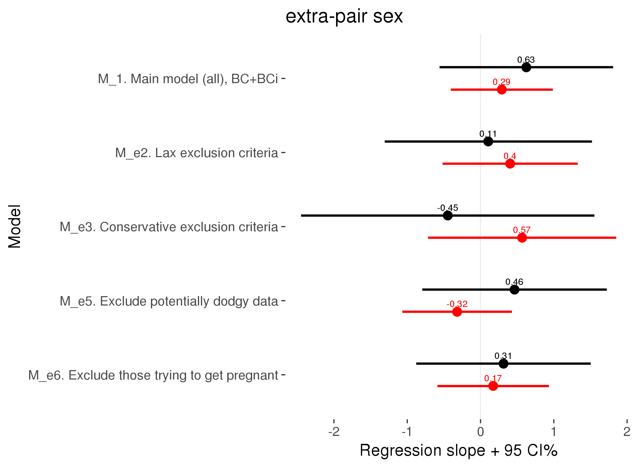
M_p: Predictors
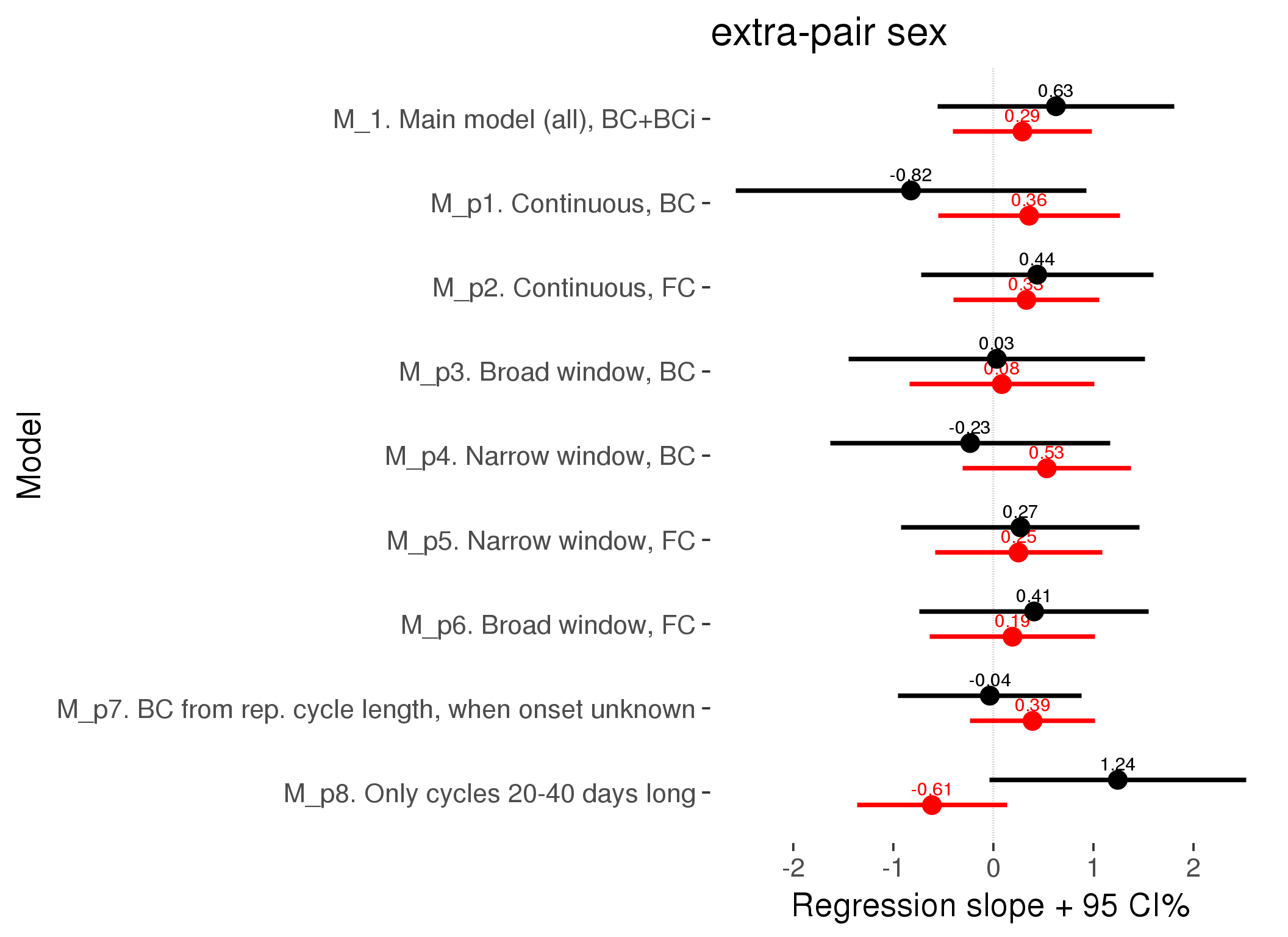
M_c: Covariates, controls, autocorrelation
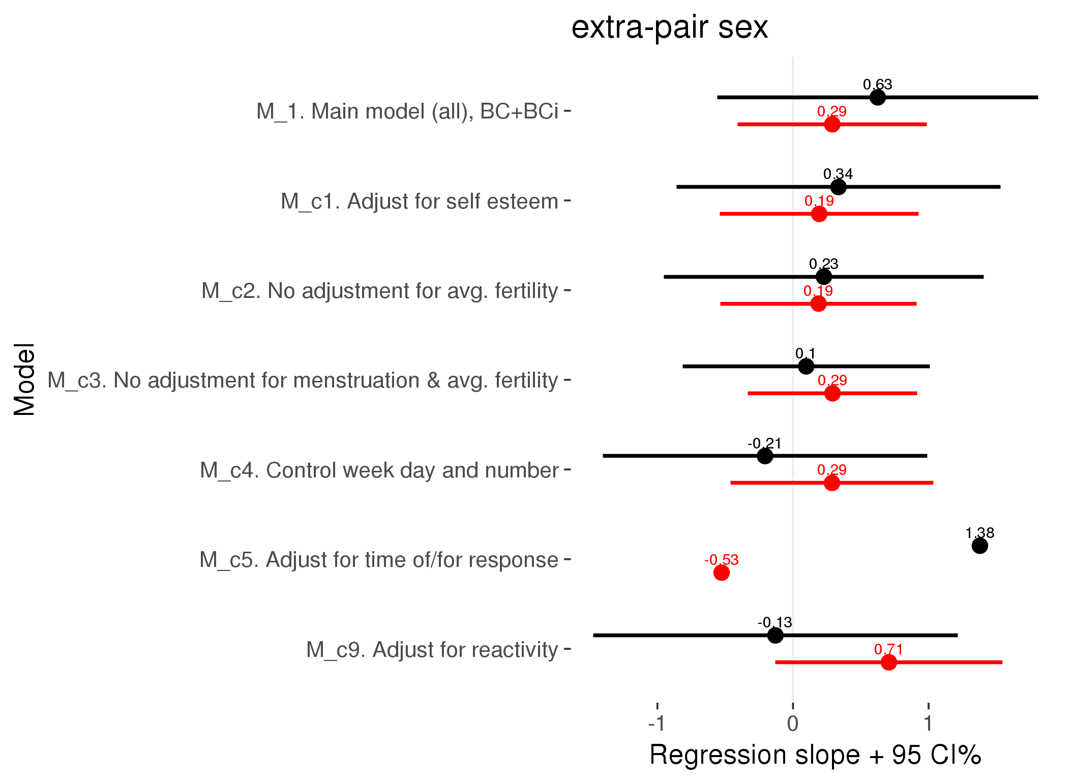
Generalized linear mixed model fit by maximum likelihood (Laplace Approximation) ['glmerMod']
 Family: binomial  ( probit )

     AIC      BIC   logLik deviance df.resid
   829.1    975.3   -396.5    793.1    24924

Scaled residuals:
   Min     1Q Median     3Q    Max
-0.738 -0.001 -0.001 -0.001  9.376

Random effects:
 Groups Name                                   Variance Std.Dev.
 person (Intercept)                            9.153442 3.0255
 Xr.2   s(days_filled_out):includedhorm_contra 0.008261 0.0909
 Xr.1   s(days_filled_out):includedcycling     0.000955 0.0309
 Xr.0   s(day_number):includedhorm_contra      0.003762 0.0613
 Xr     s(day_number):includedcycling          0.030161 0.1737
Number of obs: 24942, groups:  person, 1054; Xr.2, 8; Xr.1, 8; Xr.0, 8; Xr, 8

Fixed effects:
                                           Estimate Std. Error z value Pr(>|z|)
X(Intercept)                                 -4.680      0.466  -10.05   <2e-16 ***
Xincludedhorm_contra                         -0.124      0.356   -0.35    0.728
Xmenstruationpre                              0.253      0.196    1.29    0.197
Xmenstruationyes                             -0.217      0.234   -0.93    0.352
Xfertile                                      0.707      0.427    1.66    0.098 .
Xfertile_mean                                -0.893      2.318   -0.39    0.700
Xincludedhorm_contra:menstruationpre         -0.306      0.370   -0.83    0.408
Xincludedhorm_contra:menstruationyes         -0.142      0.448   -0.32    0.751
Xincludedhorm_contra:fertile                 -0.130      0.686   -0.19    0.850
Xs(day_number):includedcyclingFx1            -0.351      0.339   -1.04    0.301
Xs(day_number):includedhorm_contraFx1         0.339      0.288    1.18    0.239
Xs(days_filled_out):includedcyclingFx1        0.430      0.334    1.29    0.198
Xs(days_filled_out):includedhorm_contraFx1   -0.263      0.297   -0.88    0.377
---
Signif. codes:  0 '***' 0.001 '**' 0.01 '*' 0.05 '.' 0.1 ' ' 1
convergence code: 0
failure to converge in 10000 evaluations
Family: binomial
Link function: probit

Formula:
extra_pair_sex ~ included + menstruation + fertile + fertile_mean +
    s(day_number, by = included) + s(days_filled_out, by = included) +
    included:menstruation + included:fertile

Parametric coefficients:
                                    Estimate Std. Error z value Pr(>|z|)
(Intercept)                           -4.680      1.066   -4.39 0.000011 ***
includedhorm_contra                   -0.124      0.941   -0.13     0.90
menstruationpre                        0.253      0.209    1.21     0.22
menstruationyes                       -0.217      0.243   -0.90     0.37
fertile                                0.707      0.461    1.54     0.12
fertile_mean                          -0.893      5.771   -0.15     0.88
includedhorm_contra:menstruationpre   -0.306      0.398   -0.77     0.44
includedhorm_contra:menstruationyes   -0.142      0.470   -0.30     0.76
includedhorm_contra:fertile           -0.130      0.755   -0.17     0.86
---
Signif. codes:  0 '***' 0.001 '**' 0.01 '*' 0.05 '.' 0.1 ' ' 1

Approximate significance of smooth terms:
                                        edf Ref.df Chi.sq p-value
s(day_number):includedcycling          1.20   1.20   0.88    0.38
s(day_number):includedhorm_contra      1.02   1.02   0.84    0.36
s(days_filled_out):includedcycling     1.01   1.01   1.46    0.23
s(days_filled_out):includedhorm_contra 1.03   1.03   0.48    0.50

R-sq.(adj) =  -0.000489
glmer.ML =  574.4  Scale est. = 1         n = 24942
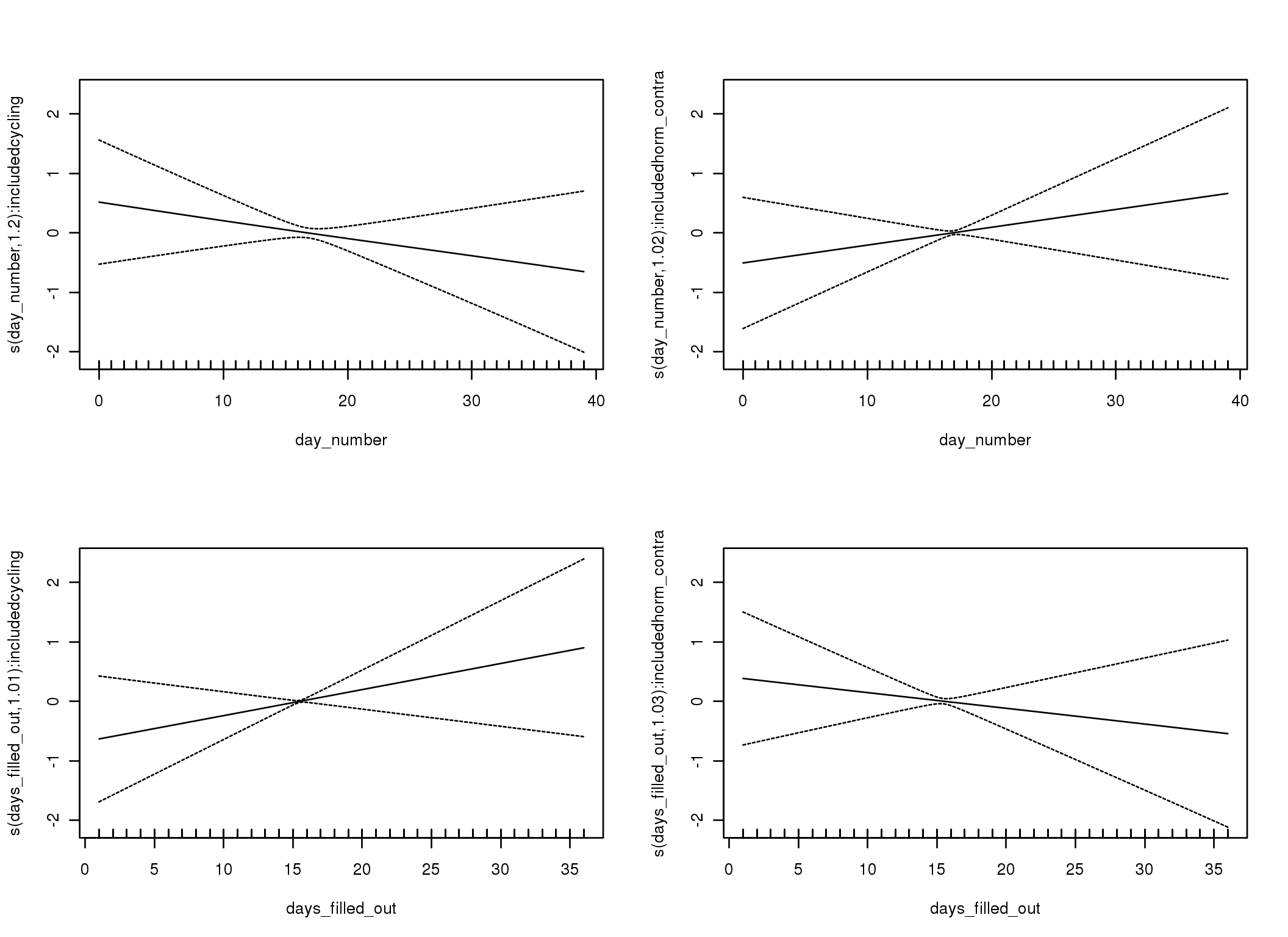
M_d: Other designs
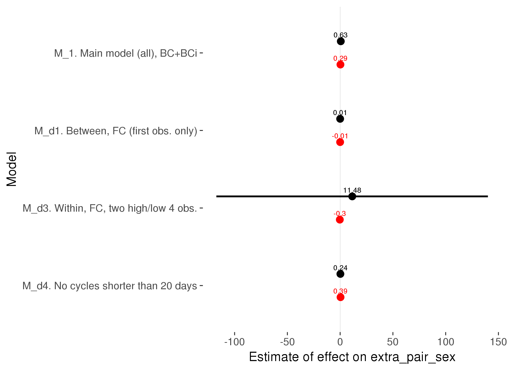
M_m1: Moderation by contraceptive method
Based on the sample with lax exclusion criteria. Users who used any hormonal contraception are classified as hormonal, users who use any awareness-based methods (counting, temperature-based) are classified as ‘fertility-awareness’, women who don’t fall into the before groups and use condoms, pessars, coitus interruptus etc. are classified as ‘barrie or abstinence’. Women who don’t use contraception or use other methods such as sterilisation are excluded from this analysis.
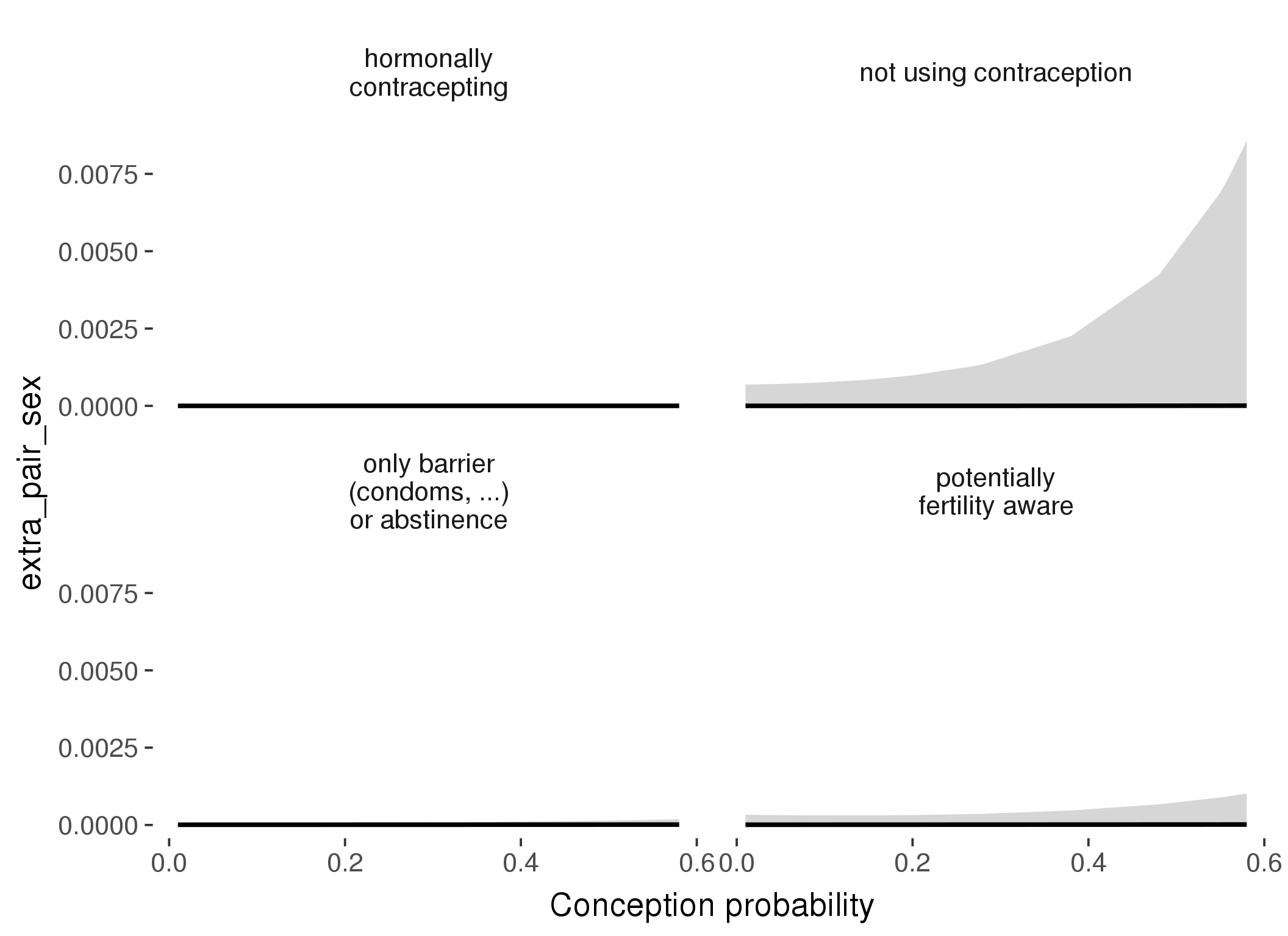
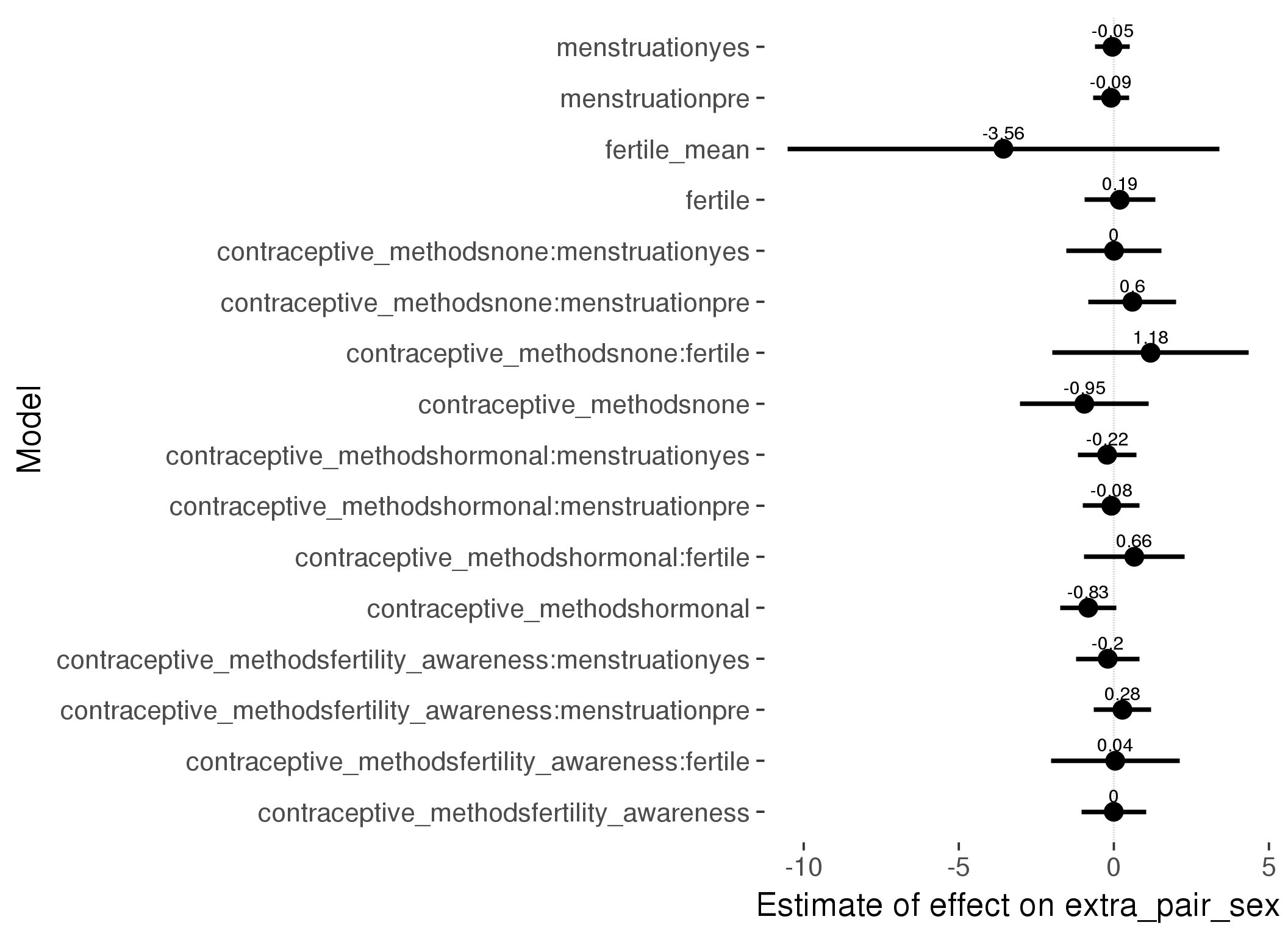
Generalized linear mixed model fit by maximum likelihood (Laplace Approximation) ['glmerMod']
 Family: binomial  ( probit )
Formula: extra_pair_sex ~ fertile_mean + (1 | person) + contraceptive_methods +
    fertile + menstruation + fertile:contraceptive_methods +      menstruation:contraceptive_methods
   Data: diary
 Subset: !is.na(included_lax) & contraceptive_method != "other"

     AIC      BIC   logLik deviance df.resid
   655.1    794.8   -309.6    619.1    17309

Scaled residuals:
   Min     1Q Median     3Q    Max
-0.796 -0.002 -0.001  0.000  8.338

Random effects:
 Groups Name        Variance Std.Dev.
 person (Intercept) 6.62     2.57
Number of obs: 17327, groups:  person, 513

Fixed effects:
                                                         Estimate Std. Error z value      Pr(>|z|)
(Intercept)                                              -3.67937    0.58125   -6.33 0.00000000024 ***
fertile_mean                                             -3.56096    3.55183   -1.00         0.316
contraceptive_methodsfertility_awareness                 -0.00439    0.53158   -0.01         0.993
contraceptive_methodsnone                                -0.95267    1.06125   -0.90         0.369
contraceptive_methodshormonal                            -0.82668    0.46450   -1.78         0.075 .
fertile                                                   0.18951    0.58182    0.33         0.745
menstruationpre                                          -0.09068    0.29507   -0.31         0.759
menstruationyes                                          -0.04614    0.28244   -0.16         0.870
contraceptive_methodsfertility_awareness:fertile          0.04392    1.05865    0.04         0.967
contraceptive_methodsnone:fertile                         1.18355    1.61484    0.73         0.464
contraceptive_methodshormonal:fertile                     0.65884    0.82474    0.80         0.424
contraceptive_methodsfertility_awareness:menstruationpre  0.27534    0.46933    0.59         0.557
contraceptive_methodsnone:menstruationpre                 0.59791    0.72170    0.83         0.407
contraceptive_methodshormonal:menstruationpre            -0.08170    0.46732   -0.17         0.861
contraceptive_methodsfertility_awareness:menstruationyes -0.19639    0.52347   -0.38         0.708
contraceptive_methodsnone:menstruationyes                 0.00423    0.78435    0.01         0.996
contraceptive_methodshormonal:menstruationyes            -0.21762    0.48104   -0.45         0.651
---
Signif. codes:  0 '***' 0.001 '**' 0.01 '*' 0.05 '.' 0.1 ' ' 1
convergence code: 0
Model failed to converge with max|grad| = 2.00364 (tol = 0.001, component 1)
| Df | AIC | BIC | logLik | deviance | Chisq | Chi Df | Pr(>Chisq) | |
|---|---|---|---|---|---|---|---|---|
| add_main | 12 | 643.2 | 736.3 | -309.6 | 619.2 | NA | NA | NA |
| by_method | 18 | 655.1 | 794.8 | -309.6 | 619.1 | 0.038 | 6 | 1 |
M_m2: Moderation by participant age
model %>%
test_moderator("age_group", diary, xlevels = 5)| Df | AIC | BIC | logLik | deviance | Chisq | Chi Df | Pr(>Chisq) | |
|---|---|---|---|---|---|---|---|---|
| with_main | 18 | 1047 | 1195 | -505.5 | 1011 | NA | NA | NA |
| with_mod | 26 | 1056 | 1270 | -502.1 | 1004 | 6.695 | 8 | 0.5698 |
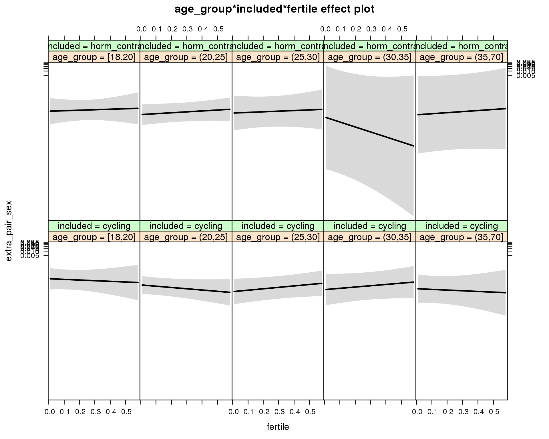
Generalized linear mixed model fit by maximum likelihood (Laplace Approximation) ['glmerMod']
 Family: binomial  ( probit )
Formula: extra_pair_sex ~ menstruation + fertile_mean + (1 | person) +
    age_group + included + fertile + menstruation:included +
    age_group:included + age_group:fertile + included:fertile +      age_group:included:fertile
   Data: diary

     AIC      BIC   logLik deviance df.resid
  1056.2   1269.8   -502.1   1004.2    27331

Scaled residuals:
   Min     1Q Median     3Q    Max
-0.741 -0.002 -0.001 -0.001  8.661

Random effects:
 Groups Name        Variance Std.Dev.
 person (Intercept) 5.63     2.37
Number of obs: 27357, groups:  person, 1054

Fixed effects:
                                             Estimate Std. Error z value Pr(>|z|)
(Intercept)                                   -3.5193     0.4103   -8.58   <2e-16 ***
menstruationpre                               -0.0393     0.1672   -0.23     0.81
menstruationyes                               -0.2822     0.1851   -1.52     0.13
fertile_mean                                  -2.1251     1.8627   -1.14     0.25
age_group(20,25]                              -0.3613     0.3809   -0.95     0.34
age_group(25,30]                              -0.7525     0.4705   -1.60     0.11
age_group(30,35]                              -0.6352     0.5476   -1.16     0.25
age_group(35,70]                              -0.5814     0.5090   -1.14     0.25
includedhorm_contra                           -0.6734     0.5050   -1.33     0.18
fertile                                       -0.3801     0.9748   -0.39     0.70
menstruationpre:includedhorm_contra           -0.1937     0.3430   -0.56     0.57
menstruationyes:includedhorm_contra           -0.1025     0.3670   -0.28     0.78
age_group(20,25]:includedhorm_contra           0.1640     0.6197    0.26     0.79
age_group(25,30]:includedhorm_contra           0.6453     0.7842    0.82     0.41
age_group(30,35]:includedhorm_contra           0.2949     1.6521    0.18     0.86
age_group(35,70]:includedhorm_contra           0.3724     1.3047    0.29     0.78
age_group(20,25]:fertile                      -0.3651     1.1212   -0.33     0.74
age_group(25,30]:fertile                       1.2138     1.1298    1.07     0.28
age_group(30,35]:fertile                       1.1354     1.2633    0.90     0.37
age_group(35,70]:fertile                      -0.0215     1.5202   -0.01     0.99
includedhorm_contra:fertile                    0.6693     1.4582    0.46     0.65
age_group(20,25]:includedhorm_contra:fertile   0.6081     1.6628    0.37     0.71
age_group(25,30]:includedhorm_contra:fertile  -1.1380     1.9084   -0.60     0.55
age_group(30,35]:includedhorm_contra:fertile  -4.3275     3.2367   -1.34     0.18
age_group(35,70]:includedhorm_contra:fertile   0.3518     2.3227    0.15     0.88
---
Signif. codes:  0 '***' 0.001 '**' 0.01 '*' 0.05 '.' 0.1 ' ' 1
convergence code: 0
Model failed to converge with max|grad| = 2.37765 (tol = 0.001, component 1)
failure to converge in 10000 evaluations
M_m3: Moderation by weekend
model %>%
test_moderator("weekend", diary, xlevels = 2) | Df | AIC | BIC | logLik | deviance | Chisq | Chi Df | Pr(>Chisq) | |
|---|---|---|---|---|---|---|---|---|
| with_main | 12 | 1025 | 1123 | -500.3 | 1001 | NA | NA | NA |
| with_mod | 14 | 1035 | 1150 | -503.5 | 1007 | 0 | 2 | 1 |
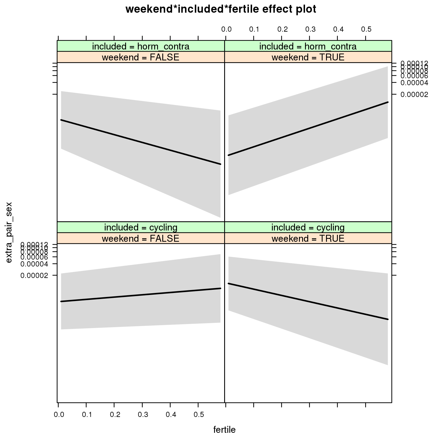
Generalized linear mixed model fit by maximum likelihood (Laplace Approximation) ['glmerMod']
 Family: binomial  ( probit )
Formula: extra_pair_sex ~ menstruation + fertile_mean + (1 | person) +
    weekend + included + fertile + menstruation:included + weekend:included +
    weekend:fertile + included:fertile + weekend:included:fertile
   Data: diary

     AIC      BIC   logLik deviance df.resid
  1035.0   1150.0   -503.5   1007.0    27343

Scaled residuals:
   Min     1Q Median     3Q    Max
-0.768 -0.003 -0.002 -0.001 12.119

Random effects:
 Groups Name        Variance Std.Dev.
 person (Intercept) 5.02     2.24
Number of obs: 27357, groups:  person, 1054

Fixed effects:
                                        Estimate Std. Error z value Pr(>|z|)
(Intercept)                               -4.371      0.352  -12.43   <2e-16 ***
menstruationpre                           -0.142      0.175   -0.81   0.4170
menstruationyes                           -0.215      0.180   -1.19   0.2334
fertile_mean                              -0.268      1.652   -0.16   0.8712
weekendTRUE                                0.265      0.158    1.68   0.0932 .
includedhorm_contra                        0.111      0.271    0.41   0.6819
fertile                                    0.323      0.443    0.73   0.4656
menstruationpre:includedhorm_contra       -0.268      0.347   -0.77   0.4395
menstruationyes:includedhorm_contra       -0.261      0.358   -0.73   0.4660
weekendTRUE:includedhorm_contra           -0.788      0.300   -2.63   0.0086 **
weekendTRUE:fertile                       -1.210      0.692   -1.75   0.0802 .
includedhorm_contra:fertile               -1.418      0.815   -1.74   0.0818 .
weekendTRUE:includedhorm_contra:fertile    3.618      1.118    3.23   0.0012 **
---
Signif. codes:  0 '***' 0.001 '**' 0.01 '*' 0.05 '.' 0.1 ' ' 1
convergence code: 0
Model failed to converge with max|grad| = 2.07465 (tol = 0.001, component 1)
M_m4: Moderation by weekday
model %>%
test_moderator("weekday", diary, xlevels = 7)| Df | AIC | BIC | logLik | deviance | Chisq | Chi Df | Pr(>Chisq) | |
|---|---|---|---|---|---|---|---|---|
| with_main | 22 | 1042 | 1223 | -499.1 | 998.3 | NA | NA | NA |
| with_mod | 34 | 1060 | 1339 | -495.8 | 991.6 | 6.694 | 12 | 0.8772 |
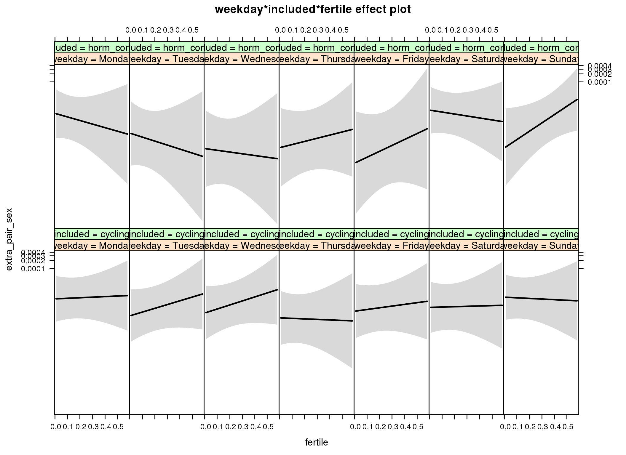
Generalized linear mixed model fit by maximum likelihood (Laplace Approximation) ['glmerMod']
 Family: binomial  ( probit )
Formula: extra_pair_sex ~ menstruation + fertile_mean + (1 | person) +
    weekday + included + fertile + menstruation:included + weekday:included +
    weekday:fertile + included:fertile + weekday:included:fertile
   Data: diary

     AIC      BIC   logLik deviance df.resid
  1059.6   1338.9   -495.8    991.6    27323

Scaled residuals:
   Min     1Q Median     3Q    Max
-0.852 -0.002 -0.001  0.000  8.526

Random effects:
 Groups Name        Variance Std.Dev.
 person (Intercept) 5.96     2.44
Number of obs: 27357, groups:  person, 1054

Fixed effects:
                                             Estimate Std. Error z value Pr(>|z|)
(Intercept)                                   -3.7105     0.3451  -10.75   <2e-16 ***
menstruationpre                                0.0421     0.1751    0.24    0.810
menstruationyes                               -0.0563     0.1786   -0.31    0.753
fertile_mean                                  -3.9966     1.9000   -2.10    0.035 *
weekdayTuesday                                -0.3831     0.2850   -1.34    0.179
weekdayWednesday                              -0.3190     0.2902   -1.10    0.272
weekdayThursday                               -0.4285     0.2923   -1.47    0.143
weekdayFriday                                 -0.2784     0.2971   -0.94    0.349
weekdaySaturday                               -0.1926     0.2844   -0.68    0.498
weekdaySunday                                  0.0382     0.2530    0.15    0.880
includedhorm_contra                            0.1108     0.3485    0.32    0.750
fertile                                        0.1286     0.7774    0.17    0.869
menstruationpre:includedhorm_contra           -0.5372     0.3688   -1.46    0.145
menstruationyes:includedhorm_contra           -0.2229     0.3393   -0.66    0.511
weekdayTuesday:includedhorm_contra            -0.0630     0.4740   -0.13    0.894
weekdayWednesday:includedhorm_contra          -0.4757     0.5326   -0.89    0.372
weekdayThursday:includedhorm_contra           -0.3465     0.5446   -0.64    0.525
weekdayFriday:includedhorm_contra             -0.8447     0.6636   -1.27    0.203
weekdaySaturday:includedhorm_contra            0.2662     0.4188    0.64    0.525
weekdaySunday:includedhorm_contra             -0.8185     0.5123   -1.60    0.110
weekdayTuesday:fertile                         0.7203     1.1048    0.65    0.514
weekdayWednesday:fertile                       0.7785     1.1132    0.70    0.484
weekdayThursday:fertile                       -0.2451     1.2812   -0.19    0.848
weekdayFriday:fertile                          0.2575     1.1497    0.22    0.823
weekdaySaturday:fertile                       -0.0474     1.2161   -0.04    0.969
weekdaySunday:fertile                         -0.2689     1.1259   -0.24    0.811
includedhorm_contra:fertile                   -0.9350     1.3555   -0.69    0.490
weekdayTuesday:includedhorm_contra:fertile    -0.8154     2.1221   -0.38    0.701
weekdayWednesday:includedhorm_contra:fertile  -0.3652     2.1535   -0.17    0.865
weekdayThursday:includedhorm_contra:fertile    1.7612     2.0743    0.85    0.396
weekdayFriday:includedhorm_contra:fertile      1.8834     2.2958    0.82    0.412
weekdaySaturday:includedhorm_contra:fertile    0.4088     1.8390    0.22    0.824
weekdaySunday:includedhorm_contra:fertile      2.9583     1.8711    1.58    0.114
---
Signif. codes:  0 '***' 0.001 '**' 0.01 '*' 0.05 '.' 0.1 ' ' 1
convergence code: 0
Model failed to converge with max|grad| = 1.98989 (tol = 0.001, component 1)
failure to converge in 10000 evaluations
M_m5: Moderation by exclusion threshold
model %>%
test_moderator("included_levels", diary, xlevels = 4)| Df | AIC | BIC | logLik | deviance | Chisq | Chi Df | Pr(>Chisq) | |
|---|---|---|---|---|---|---|---|---|
| with_main | 16 | 1031 | 1163 | -499.7 | 999.3 | NA | NA | NA |
| with_mod | 22 | 1074 | 1255 | -515 | 1030 | 0 | 6 | 1 |
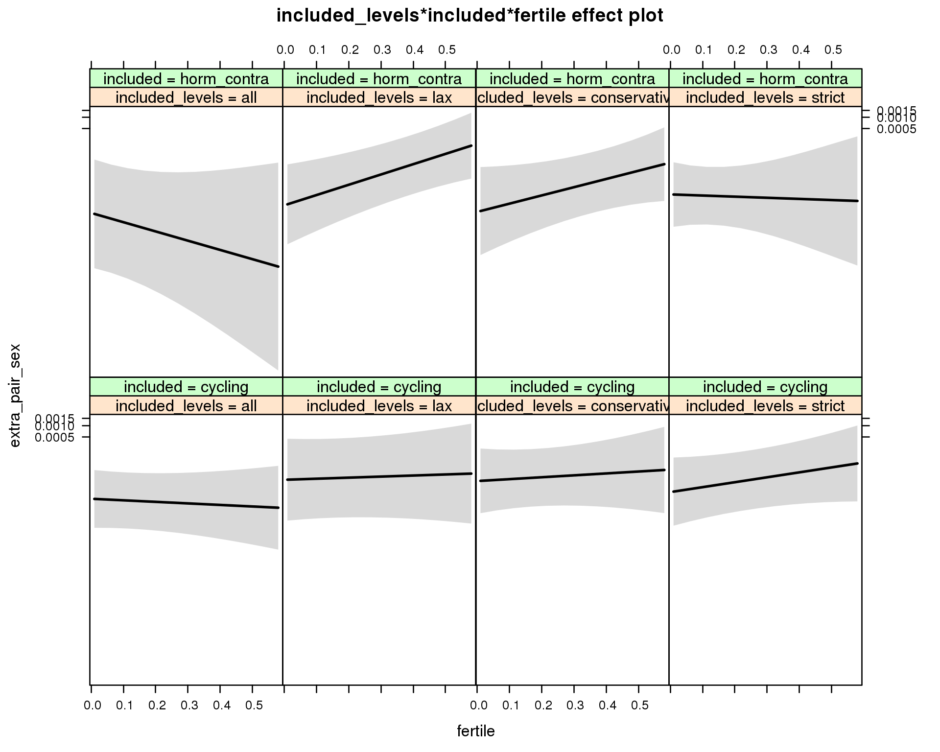
Generalized linear mixed model fit by maximum likelihood (Laplace Approximation) ['glmerMod']
 Family: binomial  ( probit )
Formula: extra_pair_sex ~ menstruation + fertile_mean + (1 | person) +
    included_levels + included + fertile + menstruation:included +
    included_levels:included + included_levels:fertile + included:fertile +
    included_levels:included:fertile
   Data: diary

     AIC      BIC   logLik deviance df.resid
    1074     1255     -515     1030    27335

Scaled residuals:
   Min     1Q Median     3Q    Max
-0.834 -0.004 -0.002 -0.001 11.074

Random effects:
 Groups Name        Variance Std.Dev.
 person (Intercept) 3.51     1.87
Number of obs: 27357, groups:  person, 1054

Fixed effects:
                                                        Estimate Std. Error z value Pr(>|z|)
(Intercept)                                              -3.6420     0.3001  -12.14   <2e-16 ***
menstruationpre                                           0.1454     0.1602    0.91    0.364
menstruationyes                                          -0.0435     0.1702   -0.26    0.798
fertile_mean                                             -4.3097     1.8020   -2.39    0.017 *
included_levelslax                                        0.3326     0.3808    0.87    0.382
included_levelsconservative                               0.3104     0.3410    0.91    0.363
included_levelsstrict                                     0.1169     0.3487    0.34    0.737
includedhorm_contra                                      -0.4082     0.4733   -0.86    0.389
fertile                                                  -0.2701     0.5945   -0.45    0.650
menstruationpre:includedhorm_contra                      -0.1117     0.3206   -0.35    0.728
menstruationyes:includedhorm_contra                       0.2045     0.3015    0.68    0.497
included_levelslax:includedhorm_contra                   -0.1995     0.6642   -0.30    0.764
included_levelsconservative:includedhorm_contra          -0.2913     0.6504   -0.45    0.654
included_levelsstrict:includedhorm_contra                 0.2081     0.6008    0.35    0.729
included_levelslax:fertile                                0.4566     0.8458    0.54    0.589
included_levelsconservative:fertile                       0.6043     0.9063    0.67    0.505
included_levelsstrict:fertile                             1.1351     0.8300    1.37    0.171
includedhorm_contra:fertile                              -1.3494     1.5917   -0.85    0.397
included_levelslax:includedhorm_contra:fertile            2.9655     1.8040    1.64    0.100
included_levelsconservative:includedhorm_contra:fertile   2.4563     1.8990    1.29    0.196
included_levelsstrict:includedhorm_contra:fertile         0.2871     2.0045    0.14    0.886
---
Signif. codes:  0 '***' 0.001 '**' 0.01 '*' 0.05 '.' 0.1 ' ' 1
convergence code: 0
Model failed to converge with max|grad| = 6.19799 (tol = 0.001, component 1)
M_m6: Moderation by cycle length
model %>%
  test_moderator("cycle_length_groups", diary, xlevels = 4)
Error: Error in pwrssUpdate(pp, resp, tol = tolPwrss, GQmat = GQmat, compDev = compDev, : (maxstephalfit) PIRLS step-halvings failed to reduce deviance in pwrssUpdate
M_m7: Moderation by certainty about menstruation parameters
model %>%
test_moderator("certainty_menstruation", diary)| Df | AIC | BIC | logLik | deviance | Chisq | Chi Df | Pr(>Chisq) | |
|---|---|---|---|---|---|---|---|---|
| with_main | 12 | 1037 | 1136 | -506.5 | 1013 | NA | NA | NA |
| with_mod | 14 | 1038 | 1153 | -504.8 | 1010 | 3.332 | 2 | 0.189 |
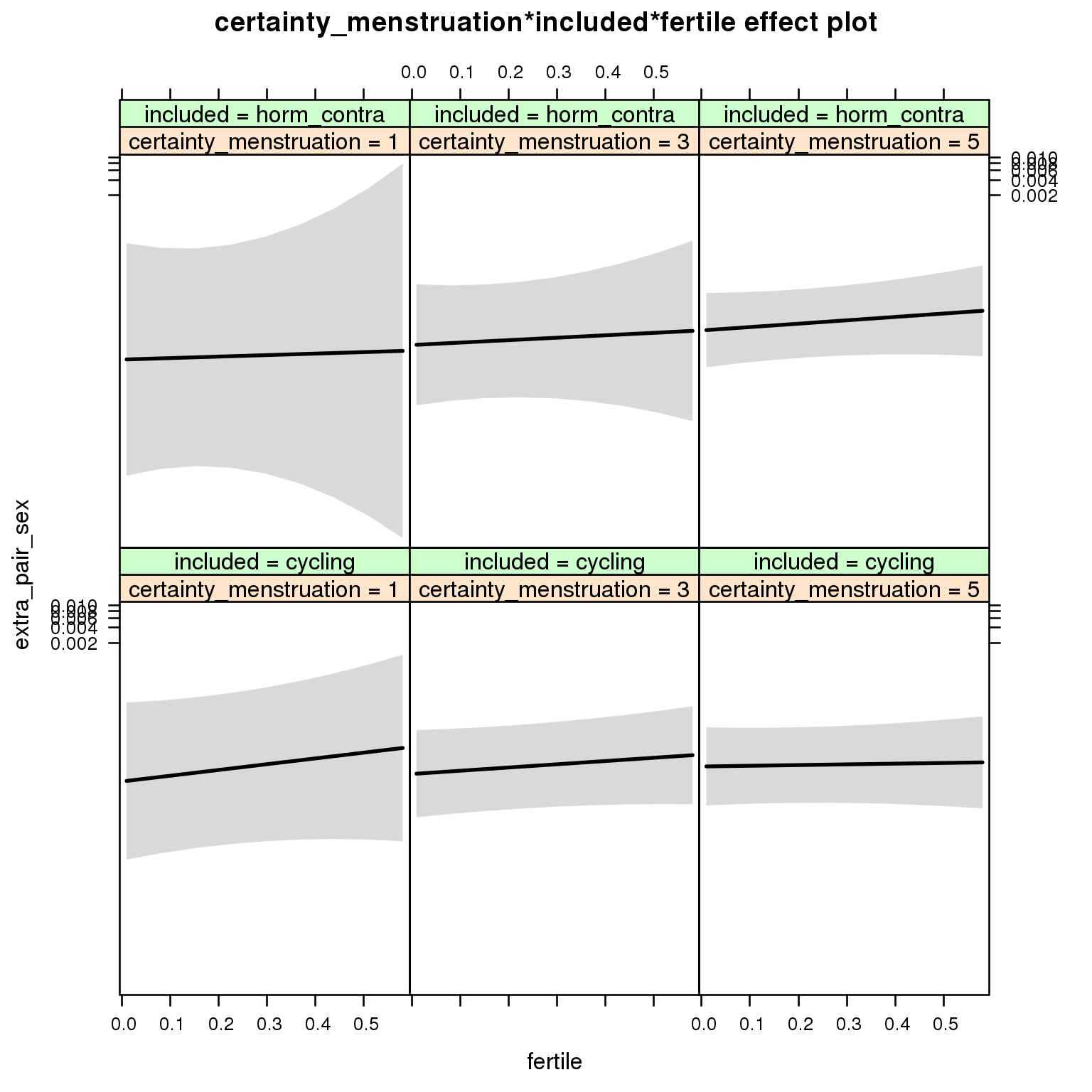
Generalized linear mixed model fit by maximum likelihood (Laplace Approximation) ['glmerMod']
 Family: binomial  ( probit )
Formula: extra_pair_sex ~ menstruation + fertile_mean + (1 | person) +
    certainty_menstruation + included + fertile + menstruation:included +
    certainty_menstruation:included + certainty_menstruation:fertile +
    included:fertile + certainty_menstruation:included:fertile
   Data: diary

     AIC      BIC   logLik deviance df.resid
  1037.7   1152.7   -504.8   1009.7    27343

Scaled residuals:
   Min     1Q Median     3Q    Max
-0.708 -0.002 -0.001 -0.001  6.945

Random effects:
 Groups Name        Variance Std.Dev.
 person (Intercept) 6.41     2.53
Number of obs: 27357, groups:  person, 1054

Fixed effects:
                                                   Estimate Std. Error z value   Pr(>|z|)
(Intercept)                                         -3.8114     0.7311   -5.21 0.00000019 ***
menstruationpre                                      0.0451     0.1696    0.27     0.7901
menstruationyes                                     -0.2813     0.1890   -1.49     0.1367
fertile_mean                                        -6.3769     2.1026   -3.03     0.0024 **
certainty_menstruation                               0.0549     0.1652    0.33     0.7394
includedhorm_contra                                 -0.4094     1.2539   -0.33     0.7440
fertile                                              1.0307     1.3236    0.78     0.4361
menstruationpre:includedhorm_contra                 -0.3293     0.3484   -0.95     0.3446
menstruationyes:includedhorm_contra                  0.2364     0.3211    0.74     0.4617
certainty_menstruation:includedhorm_contra           0.0516     0.2838    0.18     0.8558
certainty_menstruation:fertile                      -0.1855     0.3150   -0.59     0.5561
includedhorm_contra:fertile                         -0.8808     3.6341   -0.24     0.8085
certainty_menstruation:includedhorm_contra:fertile   0.2544     0.8012    0.32     0.7509
---
Signif. codes:  0 '***' 0.001 '**' 0.01 '*' 0.05 '.' 0.1 ' ' 1
convergence code: 0
Model failed to converge with max|grad| = 2.68207 (tol = 0.001, component 1)
failure to converge in 10000 evaluations
M_m8: Moderation by cycle regularity
model %>%
  test_moderator("cycle_regularity", diary)
Error: Error in pwrssUpdate(pp, resp, tol = tolPwrss, GQmat = GQmat, compDev = compDev, : Downdated VtV is not positive definite
M_m9: Moderation by cohabitation status
model %>%
test_moderator("cohabitation", diary)| Df | AIC | BIC | logLik | deviance | Chisq | Chi Df | Pr(>Chisq) | |
|---|---|---|---|---|---|---|---|---|
| with_main | 14 | 1027 | 1142 | -499.6 | 999.1 | NA | NA | NA |
| with_mod | 18 | 1046 | 1194 | -504.8 | 1010 | 0 | 4 | 1 |
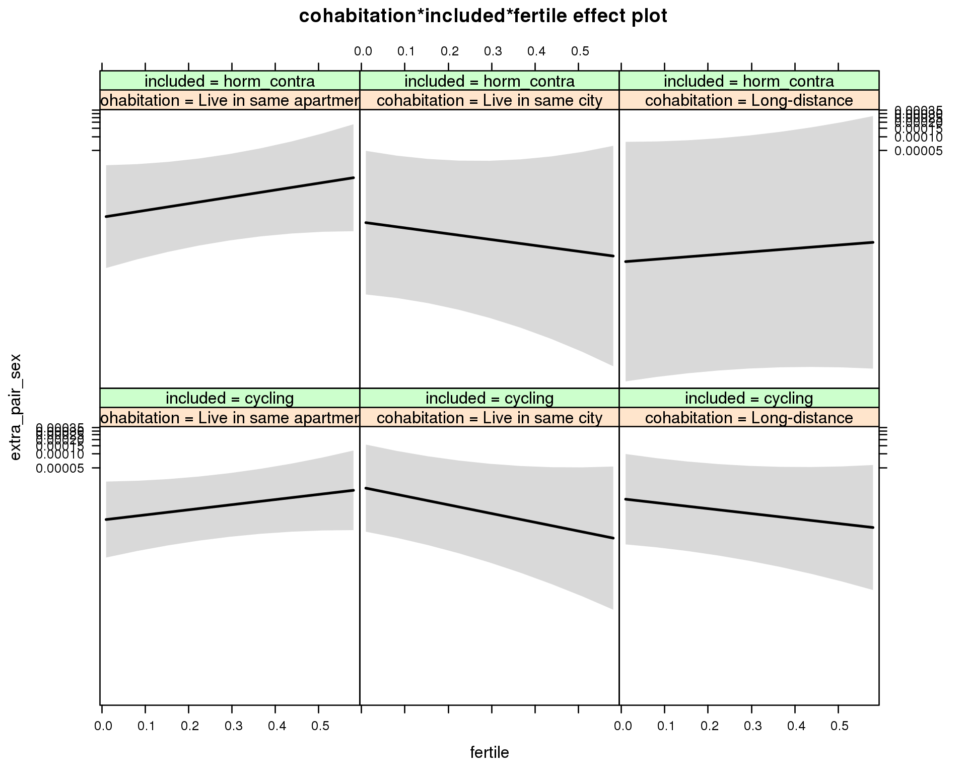
Generalized linear mixed model fit by maximum likelihood (Laplace Approximation) ['glmerMod']
 Family: binomial  ( probit )
Formula: extra_pair_sex ~ menstruation + fertile_mean + (1 | person) +
    cohabitation + included + fertile + menstruation:included +
    cohabitation:included + cohabitation:fertile + included:fertile +      cohabitation:included:fertile
   Data: diary

     AIC      BIC   logLik deviance df.resid
  1045.7   1193.6   -504.8   1009.7    27339

Scaled residuals:
   Min     1Q Median     3Q    Max
-0.740 -0.002 -0.001  0.000  7.360

Random effects:
 Groups Name        Variance Std.Dev.
 person (Intercept) 5.55     2.36
Number of obs: 27357, groups:  person, 1054

Fixed effects:
                                                          Estimate Std. Error z value Pr(>|z|)
(Intercept)                                                -4.0572     0.3676  -11.04   <2e-16 ***
menstruationpre                                            -0.1071     0.1656   -0.65    0.518
menstruationyes                                            -0.4538     0.1918   -2.37    0.018 *
fertile_mean                                               -2.2268     1.8467   -1.21    0.228
cohabitationLive in same city                               0.4074     0.3292    1.24    0.216
cohabitationLong-distance                                   0.2653     0.3363    0.79    0.430
includedhorm_contra                                        -0.2553     0.3895   -0.66    0.512
fertile                                                     0.6374     0.4973    1.28    0.200
menstruationpre:includedhorm_contra                        -0.0461     0.3486   -0.13    0.895
menstruationyes:includedhorm_contra                         0.4886     0.3359    1.45    0.146
cohabitationLive in same city:includedhorm_contra          -0.4668     0.6173   -0.76    0.450
cohabitationLong-distance:includedhorm_contra              -0.8202     0.8394   -0.98    0.329
cohabitationLive in same city:fertile                      -1.7265     0.8505   -2.03    0.042 *
cohabitationLong-distance:fertile                          -1.2545     0.7473   -1.68    0.093 .
includedhorm_contra:fertile                                 0.2102     0.8216    0.26    0.798
cohabitationLive in same city:includedhorm_contra:fertile   0.1514     1.5136    0.10    0.920
cohabitationLong-distance:includedhorm_contra:fertile       0.8268     1.2798    0.65    0.518
---
Signif. codes:  0 '***' 0.001 '**' 0.01 '*' 0.05 '.' 0.1 ' ' 1
convergence code: 0
Model failed to converge with max|grad| = 3.75735 (tol = 0.001, component 1)
failure to converge in 10000 evaluations
M_m10: Moderation by relationship status
model %>%
  test_moderator("relationship_status_clean", diary)
Error: Error in pwrssUpdate(pp, resp, tol = tolPwrss, GQmat = GQmat, compDev = compDev, : Downdated VtV is not positive definite
Does extra-pair desire predict having sex with an extra-pair mate?
diary %>%
  group_by(person) %>%
  mutate_at(vars(extra_pair_compliments, extra_pair_flirting, extra_pair_going_out),
    funs(mean, lag), na.rm = T) %>%
  glmer(extra_pair_sex ~
          extra_pair_compliments_mean + extra_pair_compliments +
          extra_pair_flirting_mean + extra_pair_flirting +
          # extra_pair_going_out_mean + extra_pair_going_out_lag + extra_pair_going_out +
          (1 | person), data = ., family = binomial(link = 'probit')) %>% summary()
## Generalized linear mixed model fit by maximum likelihood (Laplace Approximation) ['glmerMod']
## Family: binomial ( probit )
## Formula: extra_pair_sex ~ extra_pair_compliments_mean + extra_pair_compliments +
## extra_pair_flirting_mean + extra_pair_flirting + (1 | person)
## Data: .
##
## AIC BIC logLik deviance df.resid
## 983.9 1033.7 -485.9 971.9 29867
##
## Scaled residuals:
## Min 1Q Median 3Q Max
## -1.28 0.00 0.00 0.00 11.86
##
## Random effects:
## Groups Name Variance Std.Dev.
## person (Intercept) 9.06 3.01
## Number of obs: 29873, groups: person, 1154
##
## Fixed effects:
## Estimate Std. Error z value Pr(>|z|)
## (Intercept) -6.2267 0.4964 -12.54 < 2e-16 ***
## extra_pair_compliments_mean -0.3000 0.1988 -1.51 0.131
## extra_pair_compliments 0.4234 0.0552 7.68 1.6e-14 ***
## extra_pair_flirting_mean 0.3047 0.2587 1.18 0.239
## extra_pair_flirting 0.1300 0.0614 2.12 0.034 *
## ---
## Signif. codes: 0 '***' 0.001 '**' 0.01 '*' 0.05 '.' 0.1 ' ' 1
##
## Correlation of Fixed Effects:
## (Intr) extr_pr_c_ extr_pr_c extr_pr_f_
## extr_pr_cm_ -0.507
## extr_pr_cmp -0.405 -0.144
## extr_pr_fl_ -0.028 -0.698 0.141
## extr_pr_flr 0.041 0.111 -0.456 -0.299In-pair desire
model_summaries$in_pair_desireModel summary
Model summary
model %>%
  print_summary()
Linear mixed model fit by REML
t-tests use Satterthwaite approximations to degrees of freedom ['lmerMod']
Formula: in_pair_desire ~ included * (menstruation + fertile) + fertile_mean + (1 | person)
Data: diary
REML criterion at convergence: 83086
Scaled residuals:
Min 1Q Median 3Q Max
-3.481 -0.678 -0.031 0.667 3.799
Random effects:
Groups Name Variance Std.Dev.
person (Intercept) 0.736 0.858
Residual 1.189 1.090
Number of obs: 26680, groups: person, 1054
Fixed effects:
Estimate Std. Error df t value Pr(>|t|)
(Intercept) 3.47053 0.07560 1399.00000 45.91 < 2e-16 ***
includedhorm_contra 0.29330 0.06188 1365.00000 4.74 0.0000023616 ***
menstruationpre -0.06767 0.03327 26000.00000 -2.03 0.0419 *
menstruationyes -0.18759 0.03135 26112.00000 -5.98 0.0000000022 ***
fertile 0.26125 0.06714 25981.00000 3.89 0.0001 ***
fertile_mean 0.03371 0.34713 1518.00000 0.10 0.9227
includedhorm_contra:menstruationpre -0.00281 0.04271 25996.00000 -0.07 0.9475
includedhorm_contra:menstruationyes 0.03767 0.04109 26088.00000 0.92 0.3593
includedhorm_contra:fertile -0.47357 0.08505 26113.00000 -5.57 0.0000000260 ***
---
Signif. codes: 0 '***' 0.001 '**' 0.01 '*' 0.05 '.' 0.1 ' ' 1
Correlation of Fixed Effects:
(Intr) incld_ mnstrtnp mnstrtny fertil frtl_m inclddhrm_cntr:mnstrtnp
inclddhrm_c -0.473
menstrutnpr -0.170 0.215
menstrutnys -0.165 0.207 0.397
fertile -0.163 0.266 0.467 0.384
fertile_men -0.772 -0.026 -0.008 -0.005 -0.069
inclddhrm_cntr:mnstrtnp 0.140 -0.269 -0.779 -0.309 -0.363 -0.004
inclddhrm_cntr:mnstrtny 0.132 -0.254 -0.303 -0.763 -0.293 -0.004 0.383
inclddhrm_cntr:f 0.163 -0.336 -0.368 -0.303 -0.786 0.010 0.466
inclddhrm_cntr:mnstrtny
inclddhrm_c
menstrutnpr
menstrutnys
fertile
fertile_men
inclddhrm_cntr:mnstrtnp
inclddhrm_cntr:mnstrtny
inclddhrm_cntr:f 0.381
Effect size standardised by residual variance (\(\frac{b}{ SD_{residual} }\)): 0.24 [0.12;0.36].
Marginal effect plots
model %>%
  plot_all_effects()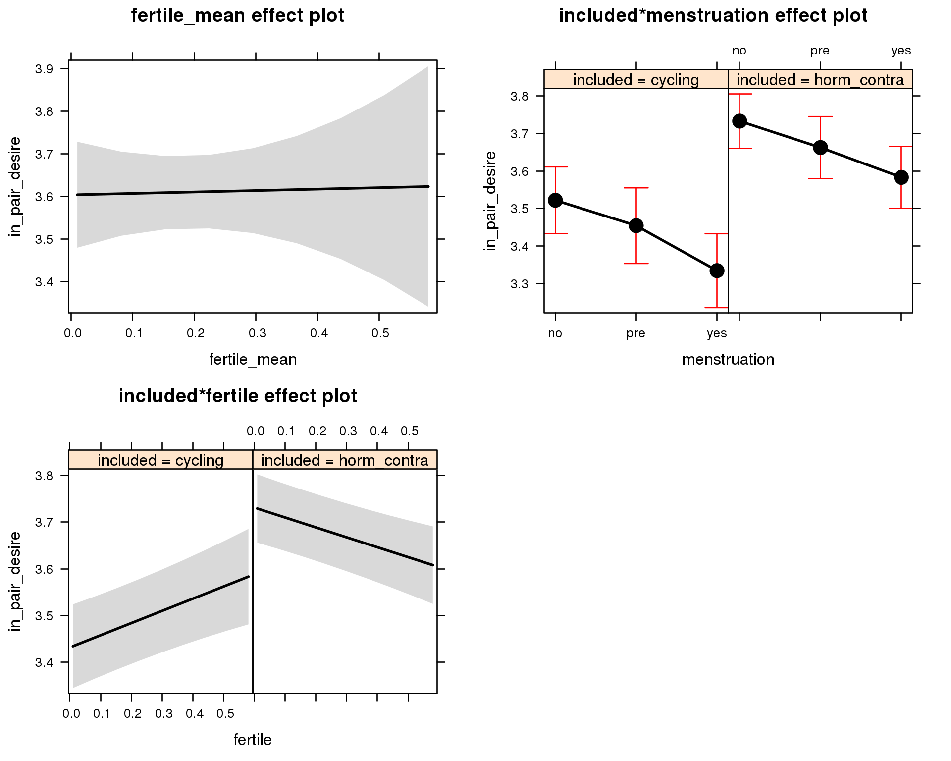
Outcome distribution
model %>%
  plot_outcome(diary) + xlab(outcome_label)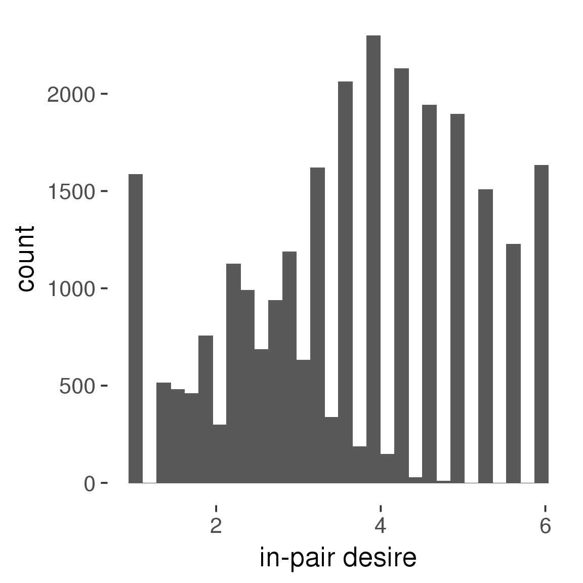
Diagnostics
model %>%
  print_diagnostics()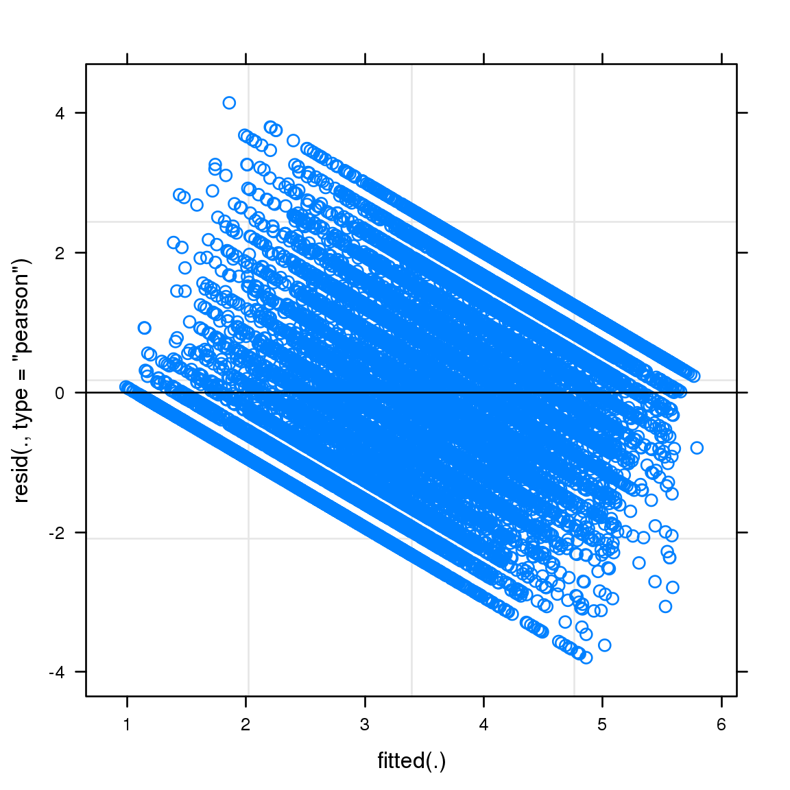
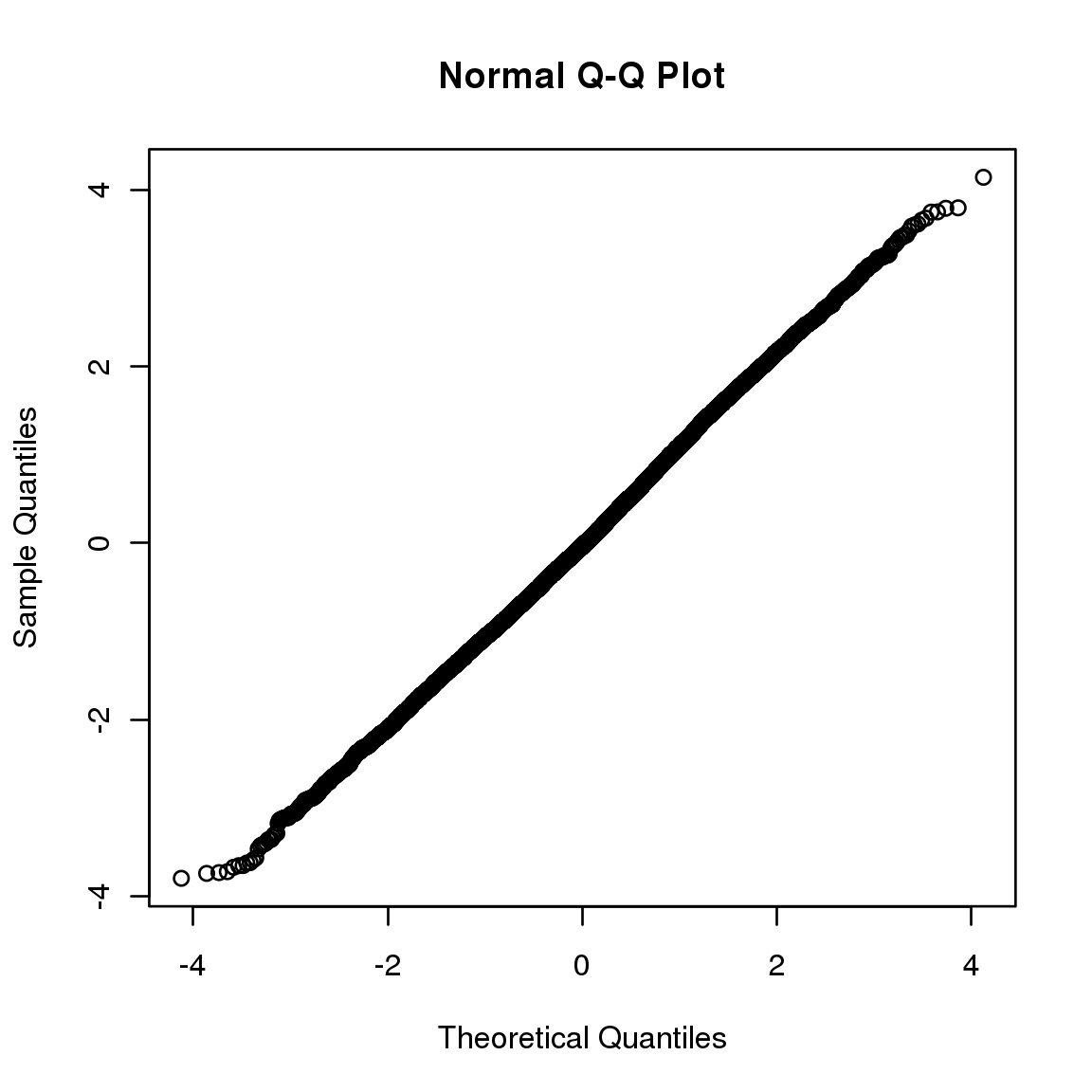

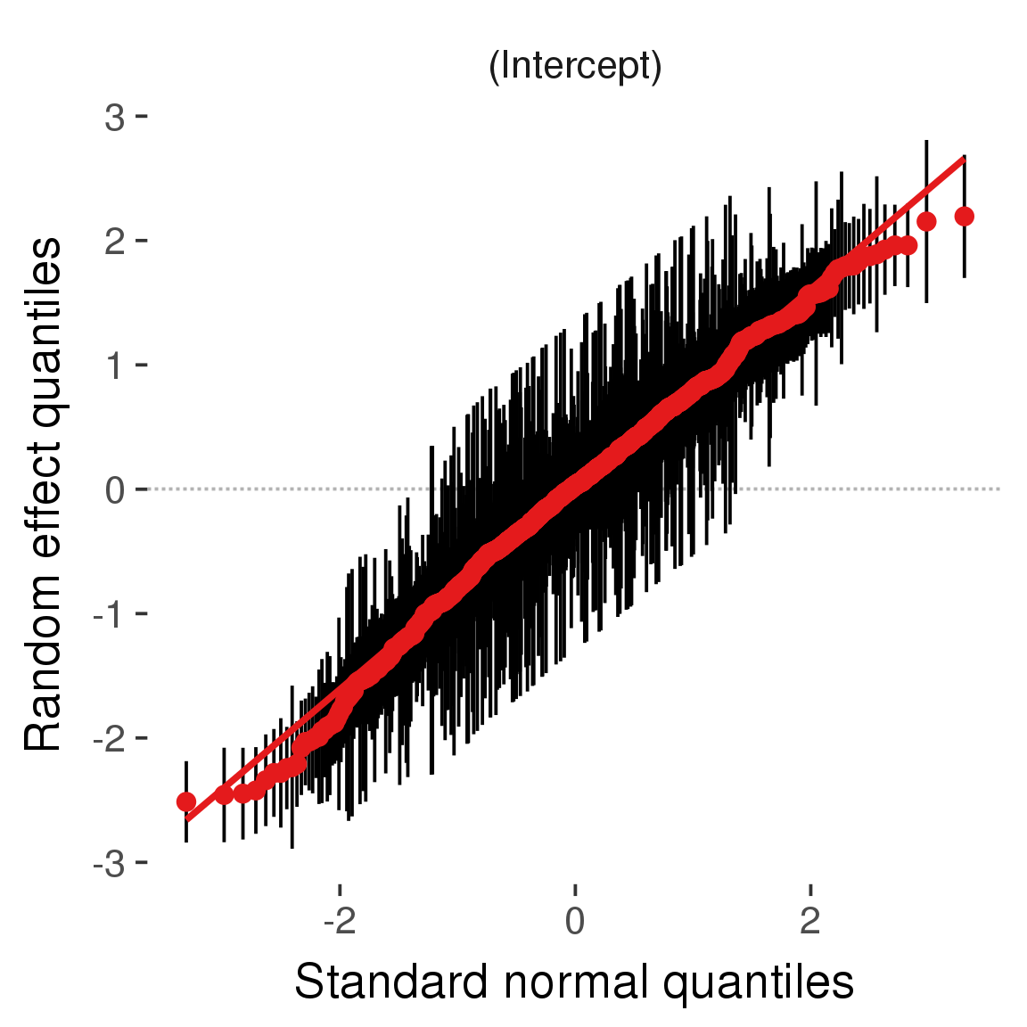
Curves
Here, we continuously plot the outcome over the course of the cycle. Because cycle lengths vary, we subset the data to cycles in a certain range. If the red curve traces the pink curve, our predictor accurately maps the relationship between fertile window probability and the outcome.
Cycle lengths from 21 to 36
Backward-counted
model %>%
  plot_curve(diary %>% filter(minimum_cycle_length_diary <= 36, minimum_cycle_length_diary > 20) %>% mutate(fertile=prc_stirn_b))
outcome = names(model@frame)[1]
outcome_label = recode(str_replace_all(str_replace_all(str_replace_all(outcome, "_", " "), " pair", "-pair"), " 1", ""),
"desirability 1" = "self-perceived desirability",
"NARQ admiration" = "narcissistic admiration",
"NARQ rivalry" = "narcissistic rivalry",
"extra-pair" = "extra-pair desire & behaviour",
"had sexual intercourse" = "sexual intercourse")
library(ggplot2)
# form a subset and run the model without the hormonal contraception and the fertility predictors
tmp = diary %>%
filter(!is.na(fertile), !is.na(included),
RCD > -1 * minimum_cycle_length_diary, RCD > -40)
new_form = update.formula(formula(model), new = . ~ . - fertile * included)
tmp$residuals = residuals(update(model, new_form, data = tmp , na.action = na.exclude))
tmp = tmp %>%
filter(!is.na(RCD), !is.na(residuals))
rcd_min = min(tmp$RCD)
tmp$real = FALSE
tmp_before = tmp
tmp_before$RCD = tmp_before$RCD + min(tmp$RCD) - 1
tmp_after = tmp
tmp_after$RCD = tmp_after$RCD - min(tmp$RCD) + 1
tmp$real = TRUE
tmp = bind_rows(tmp_before %>% filter(RCD > rcd_min - 11), tmp, tmp_after %>% filter(RCD < 11))GAM smooth on residuals
Here, we partialled out menstruation and individual random effects, then superimposed estimated probability of being in the fertile window scaled to the range of the estimated means. To address the periodicity of the cycle, we prepended and appended ten days of the timeseries to the end and the beginning of the timeseries. We then estimated the GAM and cut off the appended subsets before plotting.
tryCatch({
trend_plot = ggplot(tmp,aes(x = RCD, y = residuals, colour = included)) +
stat_smooth(geom = 'smooth',size = 0.8, fill = "#9ECAE1", method = 'gam', formula = y ~ s(x))
}, error = function(e){cat_message(e, "danger")})
tryCatch({
trend_data = ggplot_build(trend_plot)$data[[1]]
}, error = function(e){cat_message(e, "danger")})
trend_data$RCD = round(trend_data$x)
trend_data = left_join(trend_data, tmp %>% select(real, RCD,fertile) %>% unique(), by = "RCD")
trend_data %>%
filter(real == TRUE) %>%
mutate(superimposed = ( ( (fertile - 0.01)/0.58) * (max(y)-min(y) ) ) + min(y) ) ->
trend_data
ggplot(trend_data) +
geom_ribbon(aes(x = x, ymin = ymin, ymax = ymax, fill = factor(group)), alpha = 0.2) +
geom_line(aes(x = x, y = y, colour = factor(group)), size = 0.8, stat = "identity") +
scale_x_continuous(caption_x) +
geom_line(aes(x = x, y = superimposed), color = "#a83fbf", size = 1, linetype = 'dashed') +
annotate("text",x = mean(trend_data$x), y = max(trend_data$superimposed,na.rm=T) + 0.1, label = 'superimposed fertility peak', color = "#a83fbf") +
scale_y_continuous(outcome_label) +
ggtitle("GAM smooth, residuals") +
scale_color_manual("Contraception status",values = c("2"="black","1"= "red"), labels = c("2"="hormonally\ncontracepting","1"="cycling"), guide = F) +
scale_fill_manual("Contraception status",values = c("2"="black","1"= "red"), labels = c("2"="hormonally\ncontracepting","1"="cycling"), guide = F)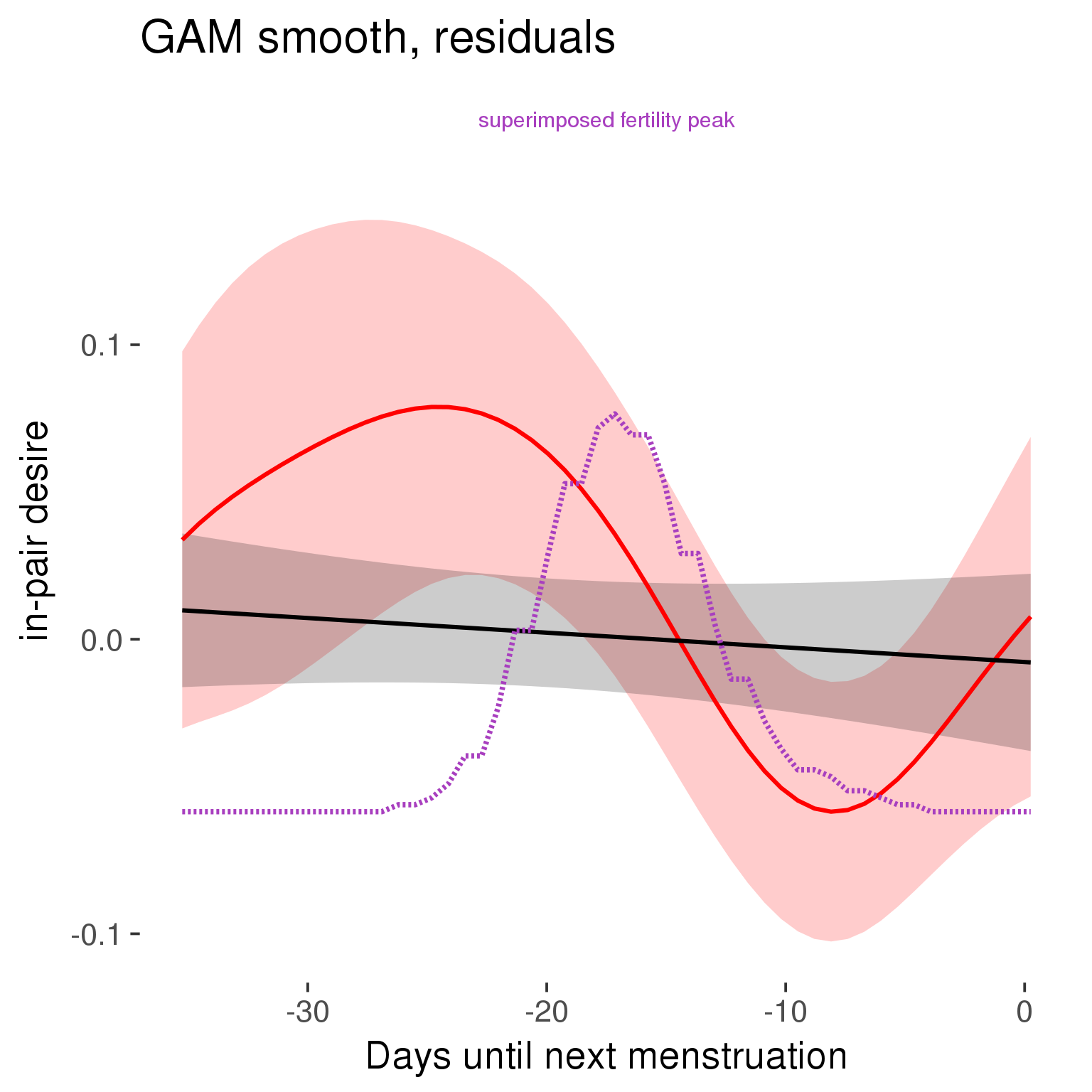
GAM smooth on raw data
As before, but without partialling anything out.
tryCatch({
trend_plot = ggplot(tmp,aes_string(x = "RCD", y = outcome, colour = "included")) +
stat_smooth(geom = 'smooth',size = 0.8, fill = "#9ECAE1", method = 'gam', formula = y ~ s(x))
}, error = function(e){cat_message(e, "danger")})
tryCatch({
trend_data = ggplot_build(trend_plot)$data[[1]]
}, error = function(e){cat_message(e, "danger")})
trend_data$RCD = round(trend_data$x)
trend_data = left_join(trend_data, tmp %>% select(real, RCD,fertile) %>% unique(), by = "RCD")
trend_data %>%
filter(real == TRUE) %>%
mutate(superimposed = ( ( (fertile - 0.01)/0.58) * (max(y)-min(y) ) ) + min(y) ) ->
trend_data
plot1b = ggplot(trend_data) +
geom_ribbon(aes(x = x, ymin = ymin, ymax = ymax, fill = factor(group)), alpha = 0.2) +
geom_line(aes(x = x, y = y, colour = factor(group)), size = 0.8, stat = "identity") +
scale_x_continuous(caption_x) +
geom_line(aes(x = x, y = superimposed), color = "#a83fbf", size = 1, linetype = 'dashed') +
annotate("text",x = mean(trend_data$x), y = max(trend_data$superimposed,na.rm=T) + 0.1, label = 'superimposed fertility peak', color = "#a83fbf") +
scale_y_continuous(outcome_label) +
ggtitle("GAM smooth, raw data") +
scale_color_manual("Contraception status",values = c("2"="black","1"= "red"), labels = c("2"="hormonally\ncontracepting","1"="cycling"), guide = F) +
scale_fill_manual("Contraception status",values = c("2"="black","1"= "red"), labels = c("2"="hormonally\ncontracepting","1"="cycling"), guide = F)
suppressWarnings(print(plot1b))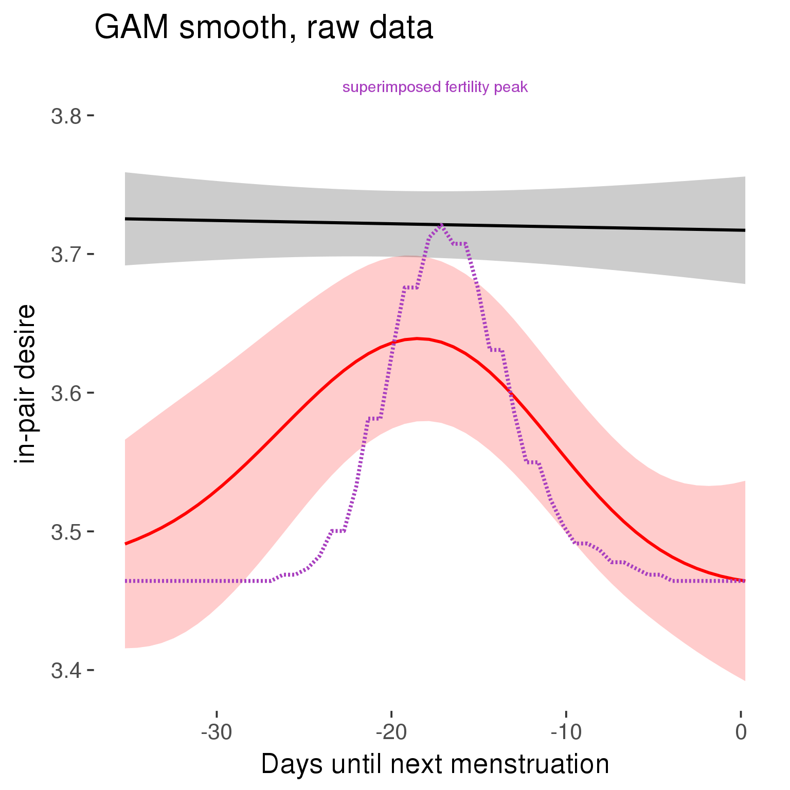
Means and standard errors over raw data
Nothing partialled out, just straight means with bootstrapped confidence intervals.
tryCatch({
trend_plot = ggplot(tmp,aes_string(x = "RCD", y = outcome, colour = "included")) +
geom_pointrange(size = 0.8, stat = 'summary', fun.data = "mean_cl_boot")
}, error = function(e){cat_message(e, "danger")})
tryCatch({
trend_data = ggplot_build(trend_plot)$data[[1]]
}, error = function(e){cat_message(e, "danger")})
trend_data$RCD = round(trend_data$x)
trend_data = left_join(trend_data, tmp %>% select(real, RCD,fertile) %>% unique(), by = "RCD")
trend_data %>%
filter(real == TRUE) %>%
mutate(superimposed = ( ( (fertile - 0.01)/0.58) * (max(y)-min(y) ) ) + min(y) ) ->
trend_data
plot3 = ggplot(trend_data) +
geom_pointrange(aes(x = x, y = y, ymin = ymin,ymax = ymax, colour = factor(group)), size = 0.8, stat = "identity", alpha = 0.6, position = position_dodge(width = .5)) +
scale_x_continuous("Days until next menstruation") +
geom_line(aes(x= x, y = superimposed), color = "#a83fbf", size = 1, linetype = 'dashed') +
annotate("text",x = mean(trend_data$x), y = max(trend_data$superimposed,na.rm=T) + 0.1, label = 'superimposed fertility peak', color = "#a83fbf") +
scale_y_continuous(outcome_label) +
ggtitle("Means with standard errors, raw data") +
scale_color_manual("Contraception status",values = c("2"="black","1"= "red"), labels = c("2"="hormonally\ncontracepting","1"="cycling"), guide = F) +
scale_fill_manual("Contraception status",values = c("2"="black","1"= "red"), labels = c("2"="hormonally\ncontracepting","1"="cycling"), guide = F)
suppressWarnings(print(plot3))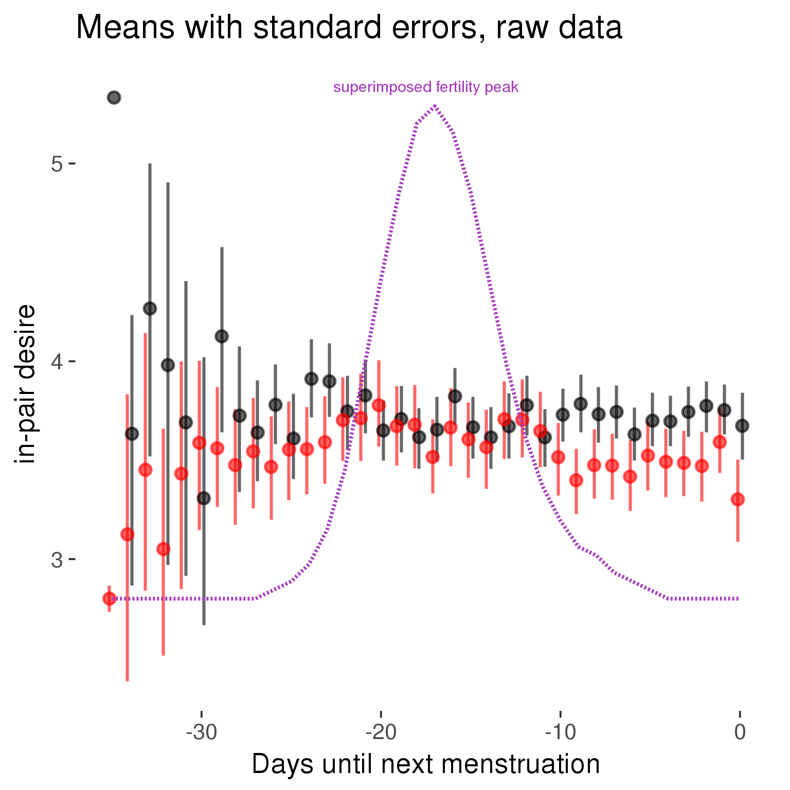
Forward-counted
model %>%
plot_curve(diary %>% filter(minimum_cycle_length_diary <= 36, minimum_cycle_length_diary > 20) %>% mutate(RCD = FCD, fertile = prc_stirn_b_forward_counted), caption_x = "Days since last menstruation")outcome = names(model@frame)[1]
outcome_label = recode(str_replace_all(str_replace_all(str_replace_all(outcome, "_", " "), " pair", "-pair"), " 1", ""),
"desirability 1" = "self-perceived desirability",
"NARQ admiration" = "narcissistic admiration",
"NARQ rivalry" = "narcissistic rivalry",
"extra-pair" = "extra-pair desire & behaviour",
"had sexual intercourse" = "sexual intercourse")
library(ggplot2)
# form a subset and run the model without the hormonal contraception and the fertility predictors
tmp = diary %>%
filter(!is.na(fertile), !is.na(included),
RCD > -1 * minimum_cycle_length_diary, RCD > -40)
new_form = update.formula(formula(model), new = . ~ . - fertile * included)
tmp$residuals = residuals(update(model, new_form, data = tmp , na.action = na.exclude))
tmp = tmp %>%
filter(!is.na(RCD), !is.na(residuals))
rcd_min = min(tmp$RCD)
tmp$real = FALSE
tmp_before = tmp
tmp_before$RCD = tmp_before$RCD + min(tmp$RCD) - 1
tmp_after = tmp
tmp_after$RCD = tmp_after$RCD - min(tmp$RCD) + 1
tmp$real = TRUE
tmp = bind_rows(tmp_before %>% filter(RCD > rcd_min - 11), tmp, tmp_after %>% filter(RCD < 11))GAM smooth on residuals
Here, we partialled out menstruation and individual random effects, then superimposed estimated probability of being in the fertile window scaled to the range of the estimated means. To address the periodicity of the cycle, we prepended and appended ten days of the timeseries to the end and the beginning of the timeseries. We then estimated the GAM and cut off the appended subsets before plotting.
tryCatch({
trend_plot = ggplot(tmp,aes(x = RCD, y = residuals, colour = included)) +
stat_smooth(geom = 'smooth',size = 0.8, fill = "#9ECAE1", method = 'gam', formula = y ~ s(x))
}, error = function(e){cat_message(e, "danger")})
tryCatch({
trend_data = ggplot_build(trend_plot)$data[[1]]
}, error = function(e){cat_message(e, "danger")})
trend_data$RCD = round(trend_data$x)
trend_data = left_join(trend_data, tmp %>% select(real, RCD,fertile) %>% unique(), by = "RCD")
trend_data %>%
filter(real == TRUE) %>%
mutate(superimposed = ( ( (fertile - 0.01)/0.58) * (max(y)-min(y) ) ) + min(y) ) ->
trend_data
ggplot(trend_data) +
geom_ribbon(aes(x = x, ymin = ymin, ymax = ymax, fill = factor(group)), alpha = 0.2) +
geom_line(aes(x = x, y = y, colour = factor(group)), size = 0.8, stat = "identity") +
scale_x_continuous(caption_x) +
geom_line(aes(x = x, y = superimposed), color = "#a83fbf", size = 1, linetype = 'dashed') +
annotate("text",x = mean(trend_data$x), y = max(trend_data$superimposed,na.rm=T) + 0.1, label = 'superimposed fertility peak', color = "#a83fbf") +
scale_y_continuous(outcome_label) +
ggtitle("GAM smooth, residuals") +
scale_color_manual("Contraception status",values = c("2"="black","1"= "red"), labels = c("2"="hormonally\ncontracepting","1"="cycling"), guide = F) +
scale_fill_manual("Contraception status",values = c("2"="black","1"= "red"), labels = c("2"="hormonally\ncontracepting","1"="cycling"), guide = F)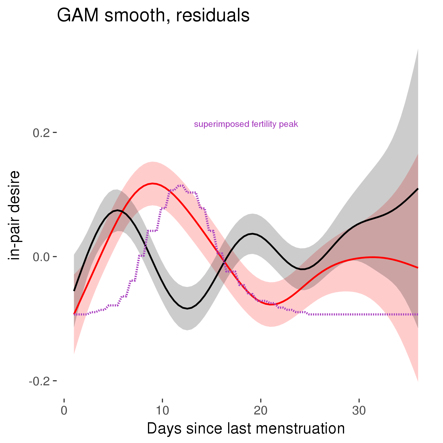
GAM smooth on raw data
As before, but without partialling anything out.
tryCatch({
trend_plot = ggplot(tmp,aes_string(x = "RCD", y = outcome, colour = "included")) +
stat_smooth(geom = 'smooth',size = 0.8, fill = "#9ECAE1", method = 'gam', formula = y ~ s(x))
}, error = function(e){cat_message(e, "danger")})
tryCatch({
trend_data = ggplot_build(trend_plot)$data[[1]]
}, error = function(e){cat_message(e, "danger")})
trend_data$RCD = round(trend_data$x)
trend_data = left_join(trend_data, tmp %>% select(real, RCD,fertile) %>% unique(), by = "RCD")
trend_data %>%
filter(real == TRUE) %>%
mutate(superimposed = ( ( (fertile - 0.01)/0.58) * (max(y)-min(y) ) ) + min(y) ) ->
trend_data
plot1b = ggplot(trend_data) +
geom_ribbon(aes(x = x, ymin = ymin, ymax = ymax, fill = factor(group)), alpha = 0.2) +
geom_line(aes(x = x, y = y, colour = factor(group)), size = 0.8, stat = "identity") +
scale_x_continuous(caption_x) +
geom_line(aes(x = x, y = superimposed), color = "#a83fbf", size = 1, linetype = 'dashed') +
annotate("text",x = mean(trend_data$x), y = max(trend_data$superimposed,na.rm=T) + 0.1, label = 'superimposed fertility peak', color = "#a83fbf") +
scale_y_continuous(outcome_label) +
ggtitle("GAM smooth, raw data") +
scale_color_manual("Contraception status",values = c("2"="black","1"= "red"), labels = c("2"="hormonally\ncontracepting","1"="cycling"), guide = F) +
scale_fill_manual("Contraception status",values = c("2"="black","1"= "red"), labels = c("2"="hormonally\ncontracepting","1"="cycling"), guide = F)
suppressWarnings(print(plot1b))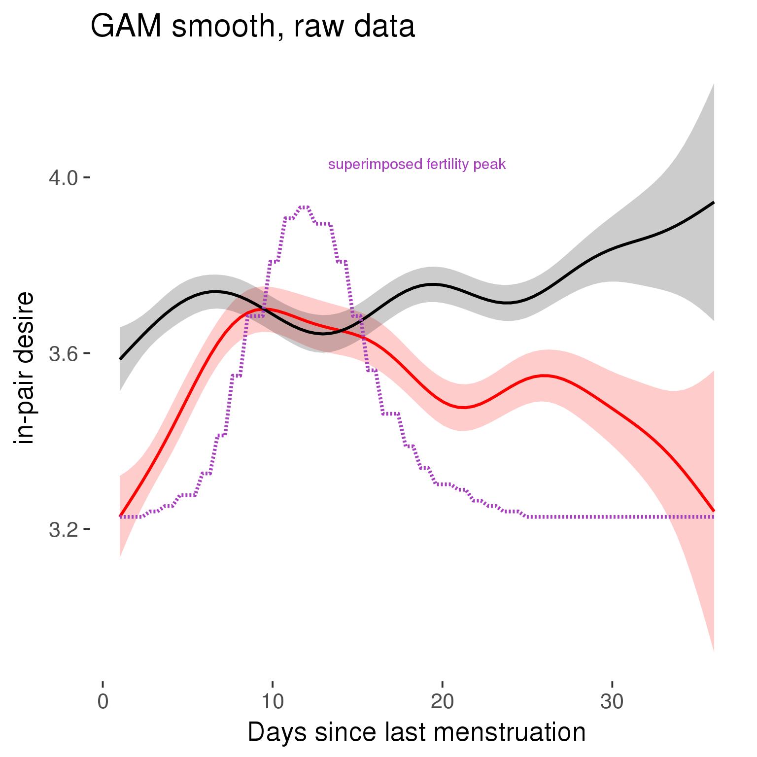
Means and standard errors over raw data
Nothing partialled out, just straight means with bootstrapped confidence intervals.
tryCatch({
trend_plot = ggplot(tmp,aes_string(x = "RCD", y = outcome, colour = "included")) +
geom_pointrange(size = 0.8, stat = 'summary', fun.data = "mean_cl_boot")
}, error = function(e){cat_message(e, "danger")})
tryCatch({
trend_data = ggplot_build(trend_plot)$data[[1]]
}, error = function(e){cat_message(e, "danger")})
trend_data$RCD = round(trend_data$x)
trend_data = left_join(trend_data, tmp %>% select(real, RCD,fertile) %>% unique(), by = "RCD")
trend_data %>%
filter(real == TRUE) %>%
mutate(superimposed = ( ( (fertile - 0.01)/0.58) * (max(y)-min(y) ) ) + min(y) ) ->
trend_data
plot3 = ggplot(trend_data) +
geom_pointrange(aes(x = x, y = y, ymin = ymin,ymax = ymax, colour = factor(group)), size = 0.8, stat = "identity", alpha = 0.6, position = position_dodge(width = .5)) +
scale_x_continuous("Days until next menstruation") +
geom_line(aes(x= x, y = superimposed), color = "#a83fbf", size = 1, linetype = 'dashed') +
annotate("text",x = mean(trend_data$x), y = max(trend_data$superimposed,na.rm=T) + 0.1, label = 'superimposed fertility peak', color = "#a83fbf") +
scale_y_continuous(outcome_label) +
ggtitle("Means with standard errors, raw data") +
scale_color_manual("Contraception status",values = c("2"="black","1"= "red"), labels = c("2"="hormonally\ncontracepting","1"="cycling"), guide = F) +
scale_fill_manual("Contraception status",values = c("2"="black","1"= "red"), labels = c("2"="hormonally\ncontracepting","1"="cycling"), guide = F)
suppressWarnings(print(plot3))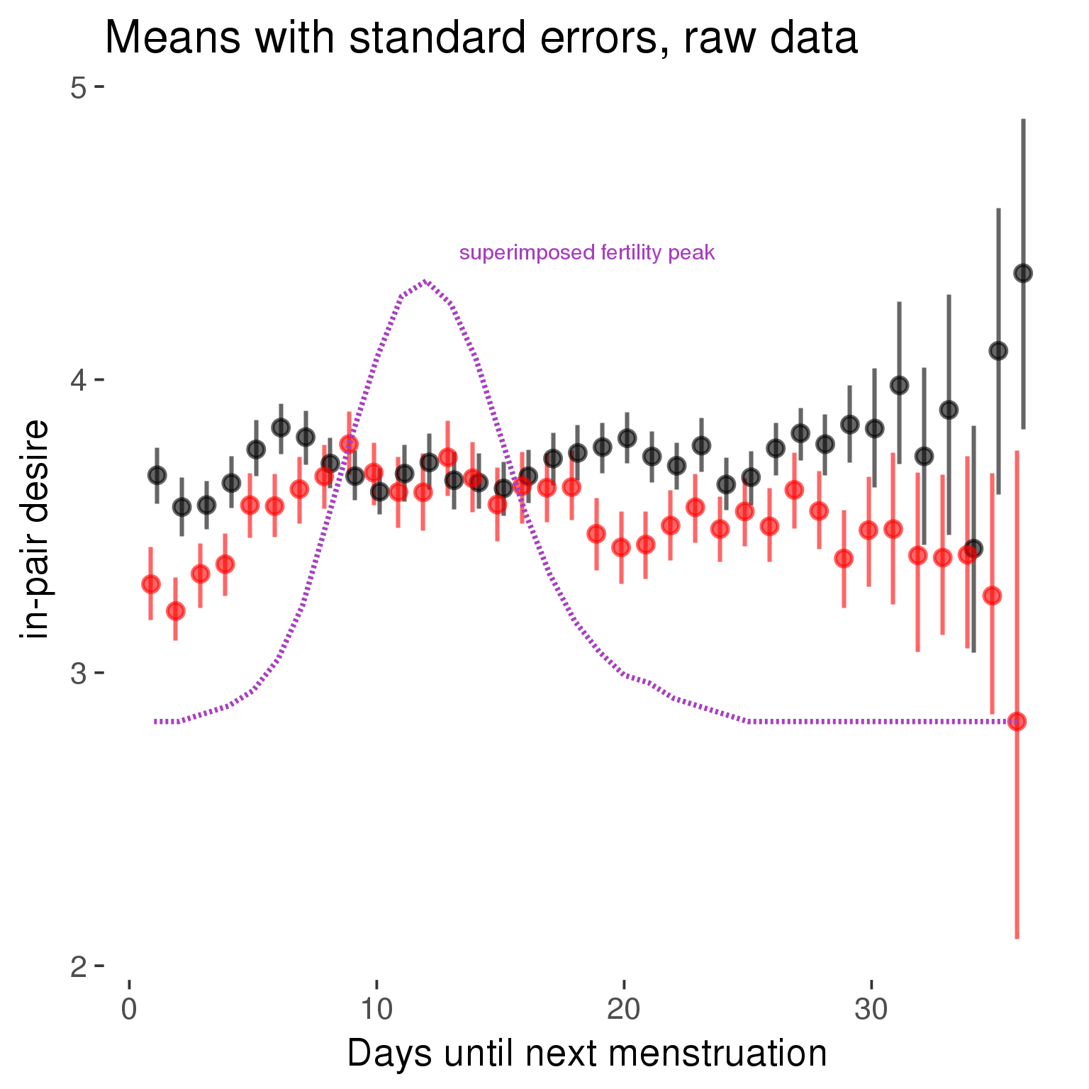
Cycle lengths from 27 to 30
Backward-counted
model %>%
plot_curve(diary %>% filter(minimum_cycle_length_diary <= 30, minimum_cycle_length_diary >= 27) %>% mutate(fertile=prc_stirn_b))outcome = names(model@frame)[1]
outcome_label = recode(str_replace_all(str_replace_all(str_replace_all(outcome, "_", " "), " pair", "-pair"), " 1", ""),
"desirability 1" = "self-perceived desirability",
"NARQ admiration" = "narcissistic admiration",
"NARQ rivalry" = "narcissistic rivalry",
"extra-pair" = "extra-pair desire & behaviour",
"had sexual intercourse" = "sexual intercourse")
library(ggplot2)
# form a subset and run the model without the hormonal contraception and the fertility predictors
tmp = diary %>%
filter(!is.na(fertile), !is.na(included),
RCD > -1 * minimum_cycle_length_diary, RCD > -40)
new_form = update.formula(formula(model), new = . ~ . - fertile * included)
tmp$residuals = residuals(update(model, new_form, data = tmp , na.action = na.exclude))
tmp = tmp %>%
filter(!is.na(RCD), !is.na(residuals))
rcd_min = min(tmp$RCD)
tmp$real = FALSE
tmp_before = tmp
tmp_before$RCD = tmp_before$RCD + min(tmp$RCD) - 1
tmp_after = tmp
tmp_after$RCD = tmp_after$RCD - min(tmp$RCD) + 1
tmp$real = TRUE
tmp = bind_rows(tmp_before %>% filter(RCD > rcd_min - 11), tmp, tmp_after %>% filter(RCD < 11))GAM smooth on residuals
Here, we partialled out menstruation and individual random effects, then superimposed estimated probability of being in the fertile window scaled to the range of the estimated means. To address the periodicity of the cycle, we prepended and appended ten days of the timeseries to the end and the beginning of the timeseries. We then estimated the GAM and cut off the appended subsets before plotting.
tryCatch({
trend_plot = ggplot(tmp,aes(x = RCD, y = residuals, colour = included)) +
stat_smooth(geom = 'smooth',size = 0.8, fill = "#9ECAE1", method = 'gam', formula = y ~ s(x))
}, error = function(e){cat_message(e, "danger")})
tryCatch({
trend_data = ggplot_build(trend_plot)$data[[1]]
}, error = function(e){cat_message(e, "danger")})
trend_data$RCD = round(trend_data$x)
trend_data = left_join(trend_data, tmp %>% select(real, RCD,fertile) %>% unique(), by = "RCD")
trend_data %>%
filter(real == TRUE) %>%
mutate(superimposed = ( ( (fertile - 0.01)/0.58) * (max(y)-min(y) ) ) + min(y) ) ->
trend_data
ggplot(trend_data) +
geom_ribbon(aes(x = x, ymin = ymin, ymax = ymax, fill = factor(group)), alpha = 0.2) +
geom_line(aes(x = x, y = y, colour = factor(group)), size = 0.8, stat = "identity") +
scale_x_continuous(caption_x) +
geom_line(aes(x = x, y = superimposed), color = "#a83fbf", size = 1, linetype = 'dashed') +
annotate("text",x = mean(trend_data$x), y = max(trend_data$superimposed,na.rm=T) + 0.1, label = 'superimposed fertility peak', color = "#a83fbf") +
scale_y_continuous(outcome_label) +
ggtitle("GAM smooth, residuals") +
scale_color_manual("Contraception status",values = c("2"="black","1"= "red"), labels = c("2"="hormonally\ncontracepting","1"="cycling"), guide = F) +
scale_fill_manual("Contraception status",values = c("2"="black","1"= "red"), labels = c("2"="hormonally\ncontracepting","1"="cycling"), guide = F)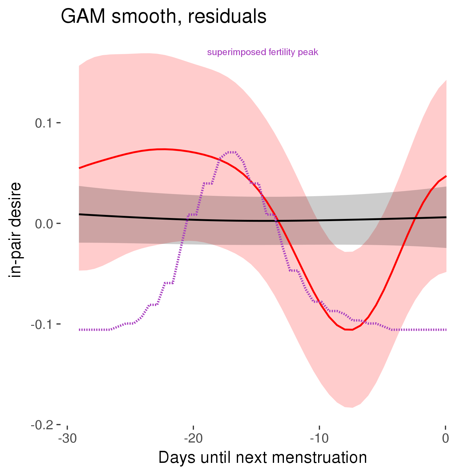
GAM smooth on raw data
As before, but without partialling anything out.
tryCatch({
trend_plot = ggplot(tmp,aes_string(x = "RCD", y = outcome, colour = "included")) +
stat_smooth(geom = 'smooth',size = 0.8, fill = "#9ECAE1", method = 'gam', formula = y ~ s(x))
}, error = function(e){cat_message(e, "danger")})
tryCatch({
trend_data = ggplot_build(trend_plot)$data[[1]]
}, error = function(e){cat_message(e, "danger")})
trend_data$RCD = round(trend_data$x)
trend_data = left_join(trend_data, tmp %>% select(real, RCD,fertile) %>% unique(), by = "RCD")
trend_data %>%
filter(real == TRUE) %>%
mutate(superimposed = ( ( (fertile - 0.01)/0.58) * (max(y)-min(y) ) ) + min(y) ) ->
trend_data
plot1b = ggplot(trend_data) +
geom_ribbon(aes(x = x, ymin = ymin, ymax = ymax, fill = factor(group)), alpha = 0.2) +
geom_line(aes(x = x, y = y, colour = factor(group)), size = 0.8, stat = "identity") +
scale_x_continuous(caption_x) +
geom_line(aes(x = x, y = superimposed), color = "#a83fbf", size = 1, linetype = 'dashed') +
annotate("text",x = mean(trend_data$x), y = max(trend_data$superimposed,na.rm=T) + 0.1, label = 'superimposed fertility peak', color = "#a83fbf") +
scale_y_continuous(outcome_label) +
ggtitle("GAM smooth, raw data") +
scale_color_manual("Contraception status",values = c("2"="black","1"= "red"), labels = c("2"="hormonally\ncontracepting","1"="cycling"), guide = F) +
scale_fill_manual("Contraception status",values = c("2"="black","1"= "red"), labels = c("2"="hormonally\ncontracepting","1"="cycling"), guide = F)
suppressWarnings(print(plot1b))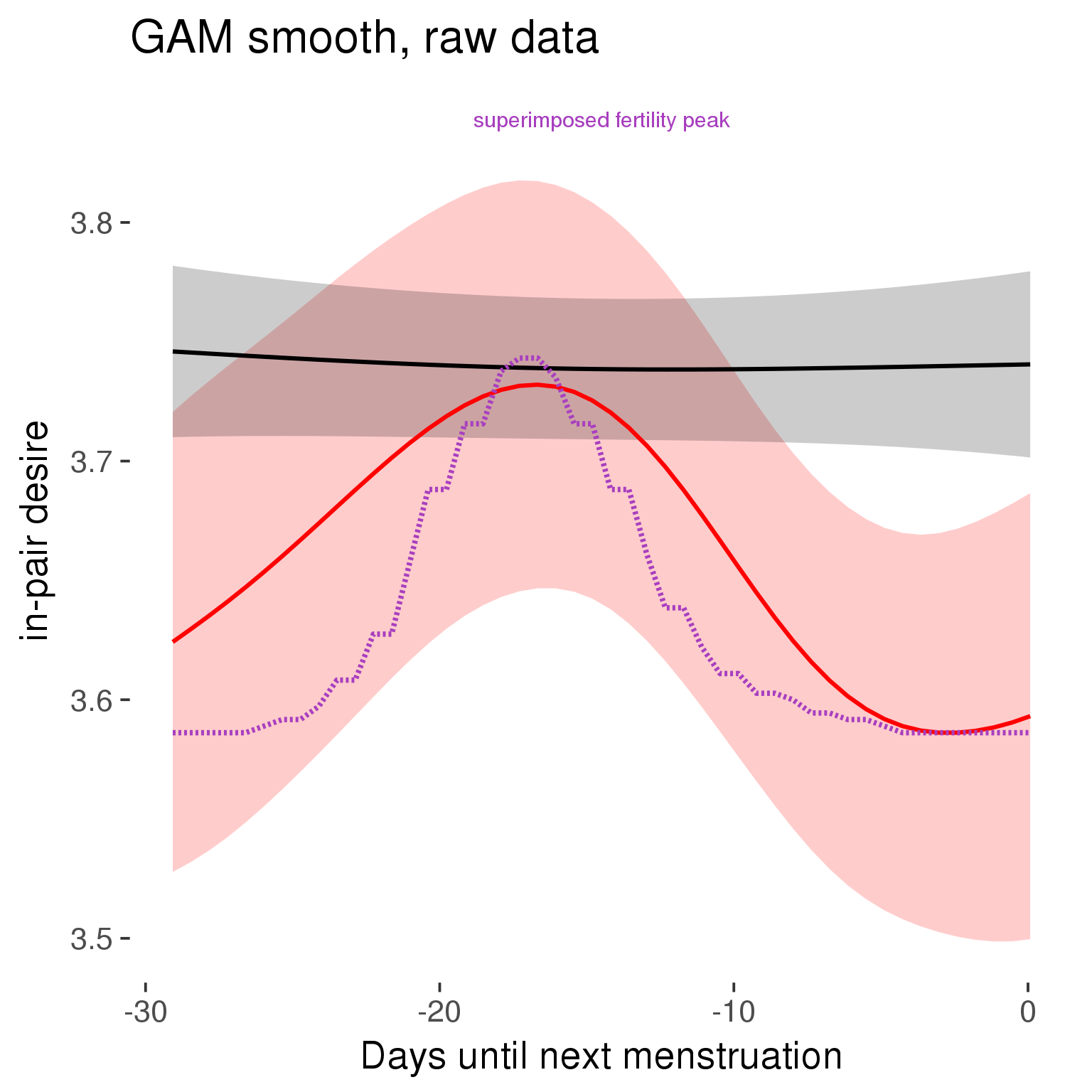
Means and standard errors over raw data
Nothing partialled out, just straight means with bootstrapped confidence intervals.
tryCatch({
trend_plot = ggplot(tmp,aes_string(x = "RCD", y = outcome, colour = "included")) +
geom_pointrange(size = 0.8, stat = 'summary', fun.data = "mean_cl_boot")
}, error = function(e){cat_message(e, "danger")})
tryCatch({
trend_data = ggplot_build(trend_plot)$data[[1]]
}, error = function(e){cat_message(e, "danger")})
trend_data$RCD = round(trend_data$x)
trend_data = left_join(trend_data, tmp %>% select(real, RCD,fertile) %>% unique(), by = "RCD")
trend_data %>%
filter(real == TRUE) %>%
mutate(superimposed = ( ( (fertile - 0.01)/0.58) * (max(y)-min(y) ) ) + min(y) ) ->
trend_data
plot3 = ggplot(trend_data) +
geom_pointrange(aes(x = x, y = y, ymin = ymin,ymax = ymax, colour = factor(group)), size = 0.8, stat = "identity", alpha = 0.6, position = position_dodge(width = .5)) +
scale_x_continuous("Days until next menstruation") +
geom_line(aes(x= x, y = superimposed), color = "#a83fbf", size = 1, linetype = 'dashed') +
annotate("text",x = mean(trend_data$x), y = max(trend_data$superimposed,na.rm=T) + 0.1, label = 'superimposed fertility peak', color = "#a83fbf") +
scale_y_continuous(outcome_label) +
ggtitle("Means with standard errors, raw data") +
scale_color_manual("Contraception status",values = c("2"="black","1"= "red"), labels = c("2"="hormonally\ncontracepting","1"="cycling"), guide = F) +
scale_fill_manual("Contraception status",values = c("2"="black","1"= "red"), labels = c("2"="hormonally\ncontracepting","1"="cycling"), guide = F)
suppressWarnings(print(plot3))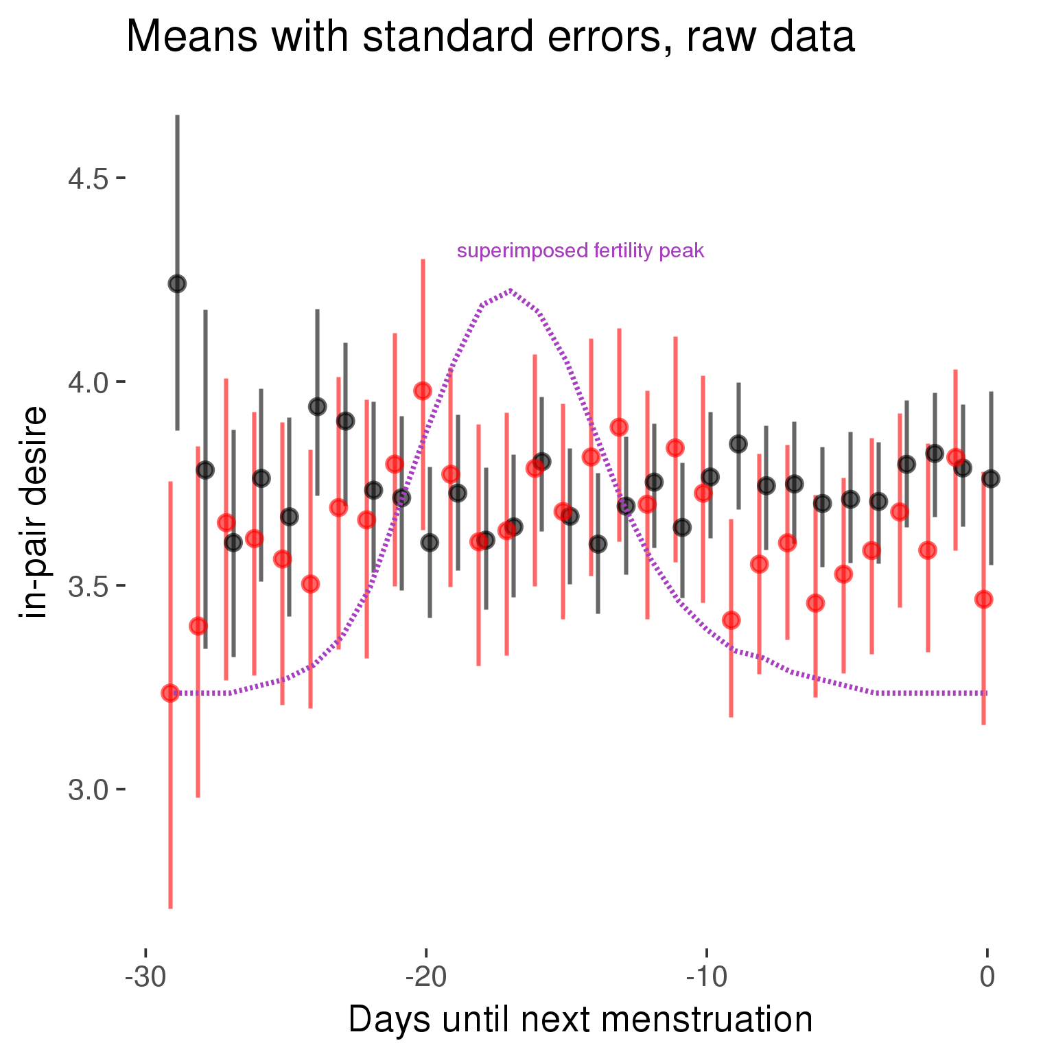
Forward-counted
model %>%
plot_curve(diary %>% filter(minimum_cycle_length_diary <= 30, minimum_cycle_length_diary >= 27) %>% mutate(RCD = FCD, fertile = prc_stirn_b_forward_counted), caption_x = "Days since last menstruation")outcome = names(model@frame)[1]
outcome_label = recode(str_replace_all(str_replace_all(str_replace_all(outcome, "_", " "), " pair", "-pair"), " 1", ""),
"desirability 1" = "self-perceived desirability",
"NARQ admiration" = "narcissistic admiration",
"NARQ rivalry" = "narcissistic rivalry",
"extra-pair" = "extra-pair desire & behaviour",
"had sexual intercourse" = "sexual intercourse")
library(ggplot2)
# form a subset and run the model without the hormonal contraception and the fertility predictors
tmp = diary %>%
filter(!is.na(fertile), !is.na(included),
RCD > -1 * minimum_cycle_length_diary, RCD > -40)
new_form = update.formula(formula(model), new = . ~ . - fertile * included)
tmp$residuals = residuals(update(model, new_form, data = tmp , na.action = na.exclude))
tmp = tmp %>%
filter(!is.na(RCD), !is.na(residuals))
rcd_min = min(tmp$RCD)
tmp$real = FALSE
tmp_before = tmp
tmp_before$RCD = tmp_before$RCD + min(tmp$RCD) - 1
tmp_after = tmp
tmp_after$RCD = tmp_after$RCD - min(tmp$RCD) + 1
tmp$real = TRUE
tmp = bind_rows(tmp_before %>% filter(RCD > rcd_min - 11), tmp, tmp_after %>% filter(RCD < 11))GAM smooth on residuals
Here, we partialled out menstruation and individual random effects, then superimposed estimated probability of being in the fertile window scaled to the range of the estimated means. To address the periodicity of the cycle, we prepended and appended ten days of the timeseries to the end and the beginning of the timeseries. We then estimated the GAM and cut off the appended subsets before plotting.
tryCatch({
trend_plot = ggplot(tmp,aes(x = RCD, y = residuals, colour = included)) +
stat_smooth(geom = 'smooth',size = 0.8, fill = "#9ECAE1", method = 'gam', formula = y ~ s(x))
}, error = function(e){cat_message(e, "danger")})
tryCatch({
trend_data = ggplot_build(trend_plot)$data[[1]]
}, error = function(e){cat_message(e, "danger")})
trend_data$RCD = round(trend_data$x)
trend_data = left_join(trend_data, tmp %>% select(real, RCD,fertile) %>% unique(), by = "RCD")
trend_data %>%
filter(real == TRUE) %>%
mutate(superimposed = ( ( (fertile - 0.01)/0.58) * (max(y)-min(y) ) ) + min(y) ) ->
trend_data
ggplot(trend_data) +
geom_ribbon(aes(x = x, ymin = ymin, ymax = ymax, fill = factor(group)), alpha = 0.2) +
geom_line(aes(x = x, y = y, colour = factor(group)), size = 0.8, stat = "identity") +
scale_x_continuous(caption_x) +
geom_line(aes(x = x, y = superimposed), color = "#a83fbf", size = 1, linetype = 'dashed') +
annotate("text",x = mean(trend_data$x), y = max(trend_data$superimposed,na.rm=T) + 0.1, label = 'superimposed fertility peak', color = "#a83fbf") +
scale_y_continuous(outcome_label) +
ggtitle("GAM smooth, residuals") +
scale_color_manual("Contraception status",values = c("2"="black","1"= "red"), labels = c("2"="hormonally\ncontracepting","1"="cycling"), guide = F) +
scale_fill_manual("Contraception status",values = c("2"="black","1"= "red"), labels = c("2"="hormonally\ncontracepting","1"="cycling"), guide = F)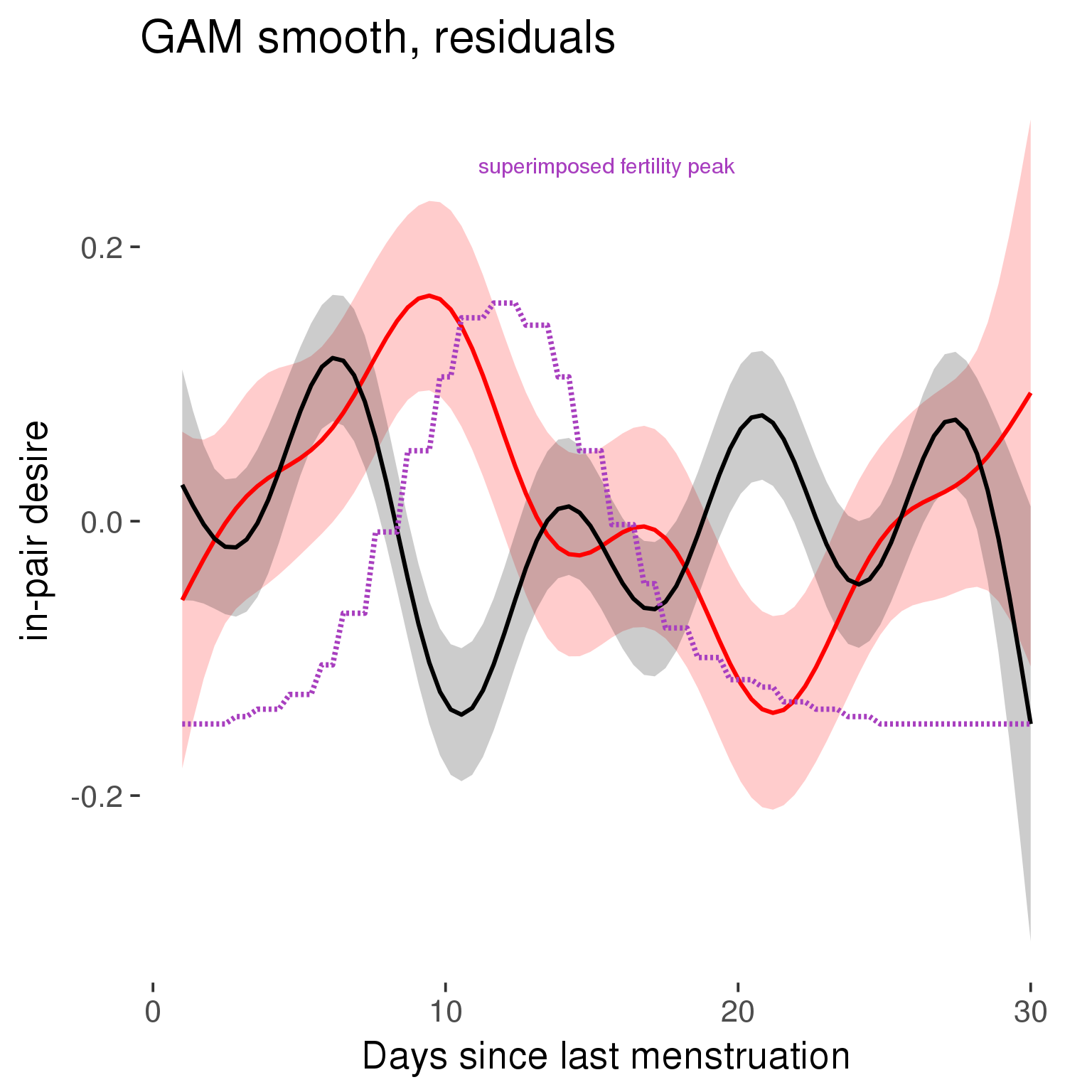
GAM smooth on raw data
As before, but without partialling anything out.
tryCatch({
trend_plot = ggplot(tmp,aes_string(x = "RCD", y = outcome, colour = "included")) +
stat_smooth(geom = 'smooth',size = 0.8, fill = "#9ECAE1", method = 'gam', formula = y ~ s(x))
}, error = function(e){cat_message(e, "danger")})
tryCatch({
trend_data = ggplot_build(trend_plot)$data[[1]]
}, error = function(e){cat_message(e, "danger")})
trend_data$RCD = round(trend_data$x)
trend_data = left_join(trend_data, tmp %>% select(real, RCD,fertile) %>% unique(), by = "RCD")
trend_data %>%
filter(real == TRUE) %>%
mutate(superimposed = ( ( (fertile - 0.01)/0.58) * (max(y)-min(y) ) ) + min(y) ) ->
trend_data
plot1b = ggplot(trend_data) +
geom_ribbon(aes(x = x, ymin = ymin, ymax = ymax, fill = factor(group)), alpha = 0.2) +
geom_line(aes(x = x, y = y, colour = factor(group)), size = 0.8, stat = "identity") +
scale_x_continuous(caption_x) +
geom_line(aes(x = x, y = superimposed), color = "#a83fbf", size = 1, linetype = 'dashed') +
annotate("text",x = mean(trend_data$x), y = max(trend_data$superimposed,na.rm=T) + 0.1, label = 'superimposed fertility peak', color = "#a83fbf") +
scale_y_continuous(outcome_label) +
ggtitle("GAM smooth, raw data") +
scale_color_manual("Contraception status",values = c("2"="black","1"= "red"), labels = c("2"="hormonally\ncontracepting","1"="cycling"), guide = F) +
scale_fill_manual("Contraception status",values = c("2"="black","1"= "red"), labels = c("2"="hormonally\ncontracepting","1"="cycling"), guide = F)
suppressWarnings(print(plot1b))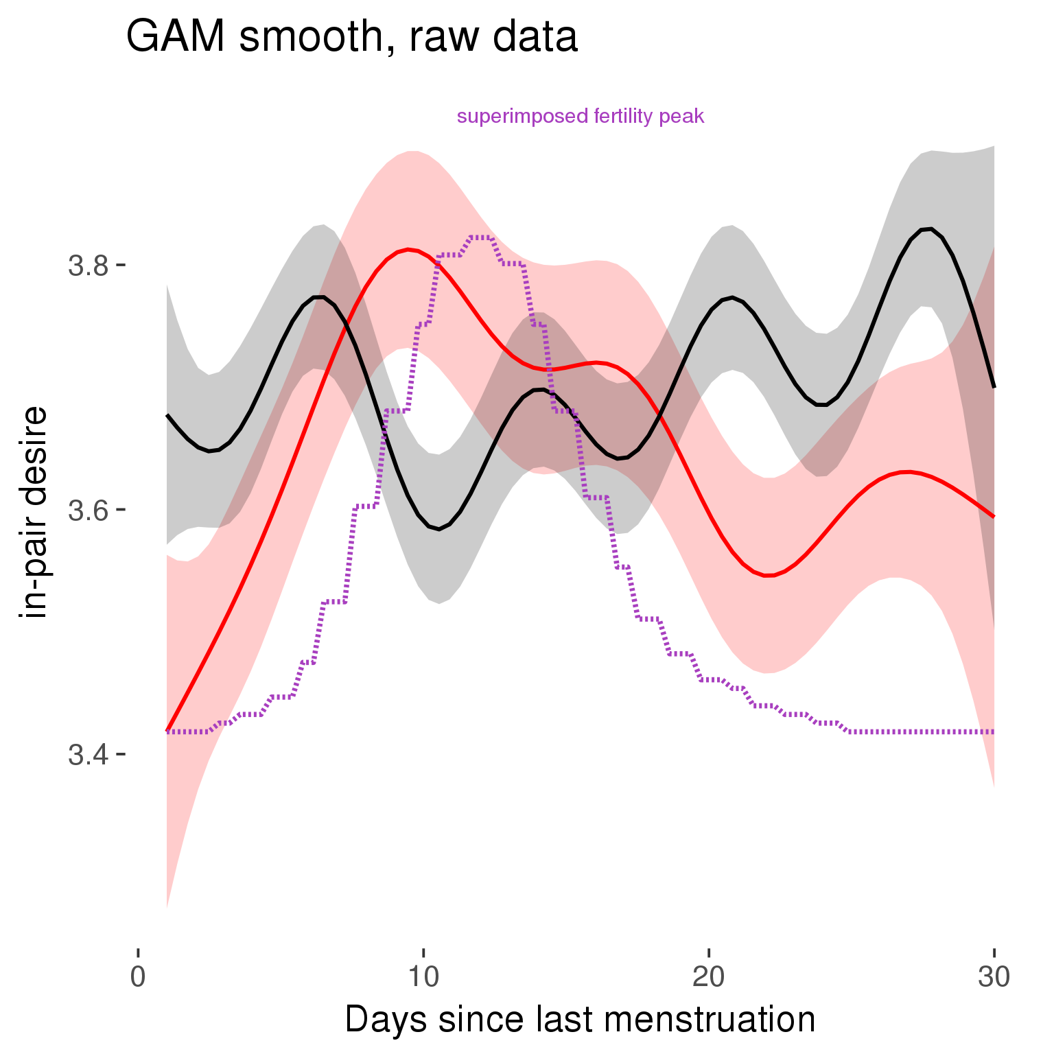
Means and standard errors over raw data
Nothing partialled out, just straight means with bootstrapped confidence intervals.
tryCatch({
trend_plot = ggplot(tmp,aes_string(x = "RCD", y = outcome, colour = "included")) +
geom_pointrange(size = 0.8, stat = 'summary', fun.data = "mean_cl_boot")
}, error = function(e){cat_message(e, "danger")})
tryCatch({
trend_data = ggplot_build(trend_plot)$data[[1]]
}, error = function(e){cat_message(e, "danger")})
trend_data$RCD = round(trend_data$x)
trend_data = left_join(trend_data, tmp %>% select(real, RCD,fertile) %>% unique(), by = "RCD")
trend_data %>%
filter(real == TRUE) %>%
mutate(superimposed = ( ( (fertile - 0.01)/0.58) * (max(y)-min(y) ) ) + min(y) ) ->
trend_data
plot3 = ggplot(trend_data) +
geom_pointrange(aes(x = x, y = y, ymin = ymin,ymax = ymax, colour = factor(group)), size = 0.8, stat = "identity", alpha = 0.6, position = position_dodge(width = .5)) +
scale_x_continuous("Days until next menstruation") +
geom_line(aes(x= x, y = superimposed), color = "#a83fbf", size = 1, linetype = 'dashed') +
annotate("text",x = mean(trend_data$x), y = max(trend_data$superimposed,na.rm=T) + 0.1, label = 'superimposed fertility peak', color = "#a83fbf") +
scale_y_continuous(outcome_label) +
ggtitle("Means with standard errors, raw data") +
scale_color_manual("Contraception status",values = c("2"="black","1"= "red"), labels = c("2"="hormonally\ncontracepting","1"="cycling"), guide = F) +
scale_fill_manual("Contraception status",values = c("2"="black","1"= "red"), labels = c("2"="hormonally\ncontracepting","1"="cycling"), guide = F)
suppressWarnings(print(plot3))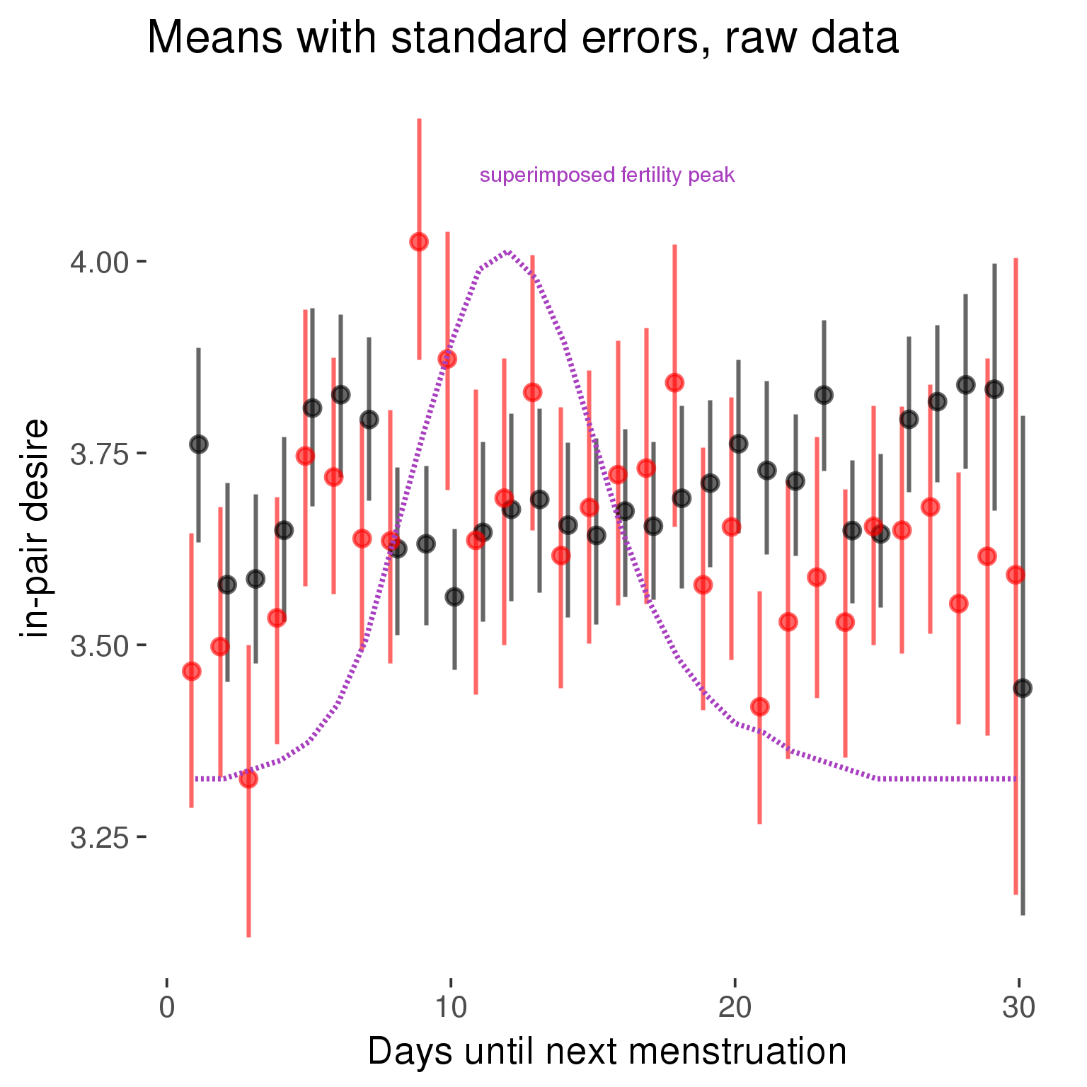
Robustness checks
M_r1: Random slopes for conception risk and menstruation
tryCatch({
# refit model with random effects for fertile and menstruation dummies
with_ind_diff = update(model, formula = . ~ . - (1| person) + (1 + fertile + menstruation | person))
# pull the random effects, format as tibble
rand = coef(with_ind_diff)$person %>%
tibble::rownames_to_column("person") %>%
mutate(person = as.numeric(person))
# pull the fixed effects
fixd = data.frame(fixef(with_ind_diff)) %>%
tibble::rownames_to_column("effect")
names(fixd) = c("effect", "pop_effect_size")
# pull apart the coefficients so that we can account for the fact that the random effect variation implicitly includes HC explaining the mean population-level effect of fertile/menstruation dummies among HC users
fixd = fixd %>%
separate(effect, c("included", "effect"), sep = ":", fill = "left") %>%
mutate(included = if_else(is.na(included), "cycling", str_replace(included, "included", "")))
fixd[2,c("included", "effect")] = c("horm_contra", "(Intercept)")
rand = rand %>%
# merge diary data on the random effects, so that we know who is a HC users and who isn't
inner_join(diary %>% select(person, included) %>% unique(), by = 'person') %>%
# gather into long format, to have the dataset by predictor
gather(effect, value, -person, -included) %>%
inner_join(fixd, by = c('effect', 'included')) %>%
# pull the fixed effects
mutate(
# only for those who are HC users, add the moderated population effect size for this effect (the random effects have the reference category mean)
value = if_else(included == "horm_contra", value + pop_effect_size, value),
effect = recode(effect, "includedhorm_contra" = "HC user",
"includedhorm_contra:fertile" = "HC user x fertile",
"includedhorm_contra:menstruationpre" = "HC user x premens.",
"includedhorm_contra:menstruationyes" = "HC user x mens.",
"menstruationyes" = "mens.",
"menstruationpre" = "premens.")) %>%
group_by(included, effect) %>%
# filter out predictors that aren't modelled as varying/random
filter(sd(value) > 0)
# plot dot plot of random effects
print(
ggplot(rand, aes(x = included, y = value, color = included, fill = included)) +
facet_wrap( ~ effect, scales = "free") +
# geom_violin(alpha = 0.4, size = 0) +
geom_dotplot(binaxis='y', dotsize = 0.1, method = "histodot") +
# geom_jitter(alpha = 0.05) +
coord_flip() +
geom_pointrange(stat = 'summary', fun.data = 'mean_sdl', color = 'darkred', size = 1.2) +
scale_color_manual("Contraception status", values = c("horm_contra"="black","cycling"= "red"), labels = c("horm_contra"="hormonally\ncontracepting","cycling"="cycling"), guide = F) +
scale_fill_manual("Contraception status", values = c("horm_contra"="black","cycling"= "red"), labels = c("horm_contra"="hormonally\ncontracepting","1"="cycling"), guide = F) +
ggtitle("M_r1: allowing participant-varying slopes", subtitle = "for the conception risk measure and the menstruation dummies") +
scale_x_discrete("Hormonal contraception", breaks = c("horm_contra", "cycling"), labels = c("yes", "no")) +
scale_y_continuous("Random effect size distribution"))
print_summary(with_ind_diff)
cat(pander(anova(model, with_ind_diff)))
}, error = function(e){
with_ind_diff = model
cat_message(e, "danger")
})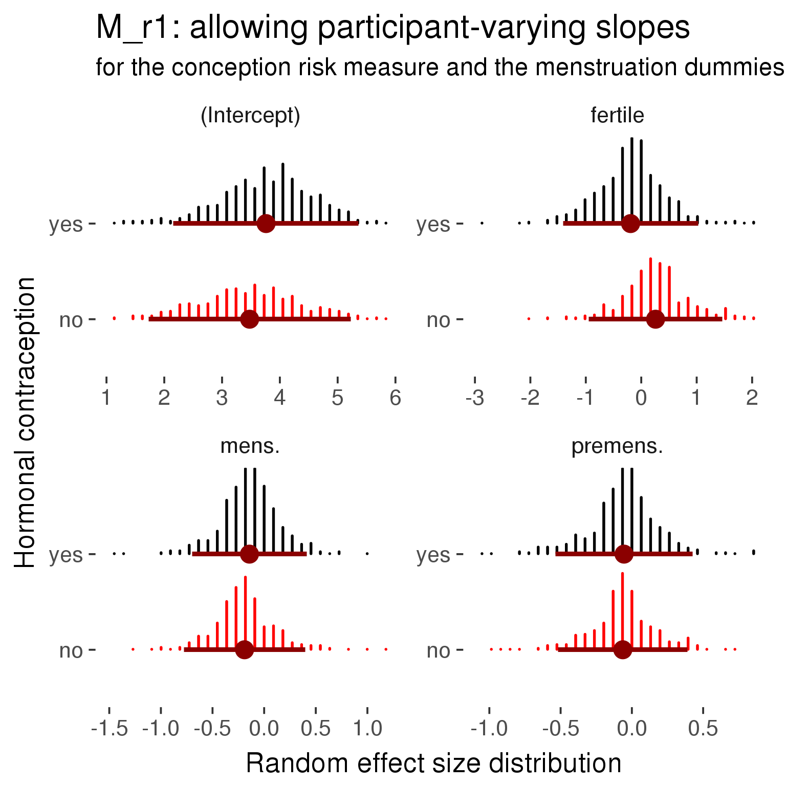
Linear mixed model fit by REML ['lmerMod']
Formula: in_pair_desire ~ included + menstruation + fertile + fertile_mean +
(1 + fertile + menstruation | person) + included:menstruation + included:fertile
Data: diary
REML criterion at convergence: 82634
Scaled residuals:
Min 1Q Median 3Q Max
-3.671 -0.661 -0.033 0.646 3.661
Random effects:
Groups Name Variance Std.Dev. Corr
person (Intercept) 0.826 0.909
fertile 1.057 1.028 -0.29
menstruationpre 0.198 0.444 -0.22 0.35
menstruationyes 0.244 0.493 -0.21 0.25 0.27
Residual 1.107 1.052
Number of obs: 26680, groups: person, 1054
Fixed effects:
Estimate Std. Error t value
(Intercept) 3.4770 0.0775 44.8
includedhorm_contra 0.2842 0.0651 4.4
menstruationpre -0.0636 0.0414 -1.5
menstruationyes -0.1899 0.0415 -4.6
fertile 0.2582 0.0876 2.9
fertile_mean 0.0146 0.3522 0.0
includedhorm_contra:menstruationpre 0.0086 0.0532 0.2
includedhorm_contra:menstruationyes 0.0476 0.0539 0.9
includedhorm_contra:fertile -0.4504 0.1113 -4.0
Correlation of Fixed Effects:
(Intr) incld_ mnstrtnp mnstrtny fertil frtl_m inclddhrm_cntr:mnstrtnp
inclddhrm_c -0.486
menstrutnpr -0.207 0.252
menstrutnys -0.205 0.245 0.335
fertile -0.213 0.329 0.410 0.325
fertile_men -0.758 -0.026 -0.005 -0.001 -0.081
inclddhrm_cntr:mnstrtnp 0.170 -0.319 -0.779 -0.261 -0.319 -0.007
inclddhrm_cntr:mnstrtny 0.162 -0.305 -0.258 -0.768 -0.249 -0.006 0.327
inclddhrm_cntr:f 0.207 -0.418 -0.323 -0.256 -0.783 0.012 0.411
inclddhrm_cntr:mnstrtny
inclddhrm_c
menstrutnpr
menstrutnys
fertile
fertile_men
inclddhrm_cntr:mnstrtnp
inclddhrm_cntr:mnstrtny
inclddhrm_cntr:f 0.322
refitting model(s) with ML (instead of REML)
| Df | AIC | BIC | logLik | deviance | Chisq | Chi Df | Pr(>Chisq) | |
|---|---|---|---|---|---|---|---|---|
| object | 11 | 83069 | 83159 | -41524 | 83047 | NA | NA | NA |
| ..1 | 20 | 82639 | 82803 | -41299 | 82599 | 448.3 | 9 | 6.694e-91 |
robustness_check_ovu_shift(model, diary)M_e: Exclusion criteria
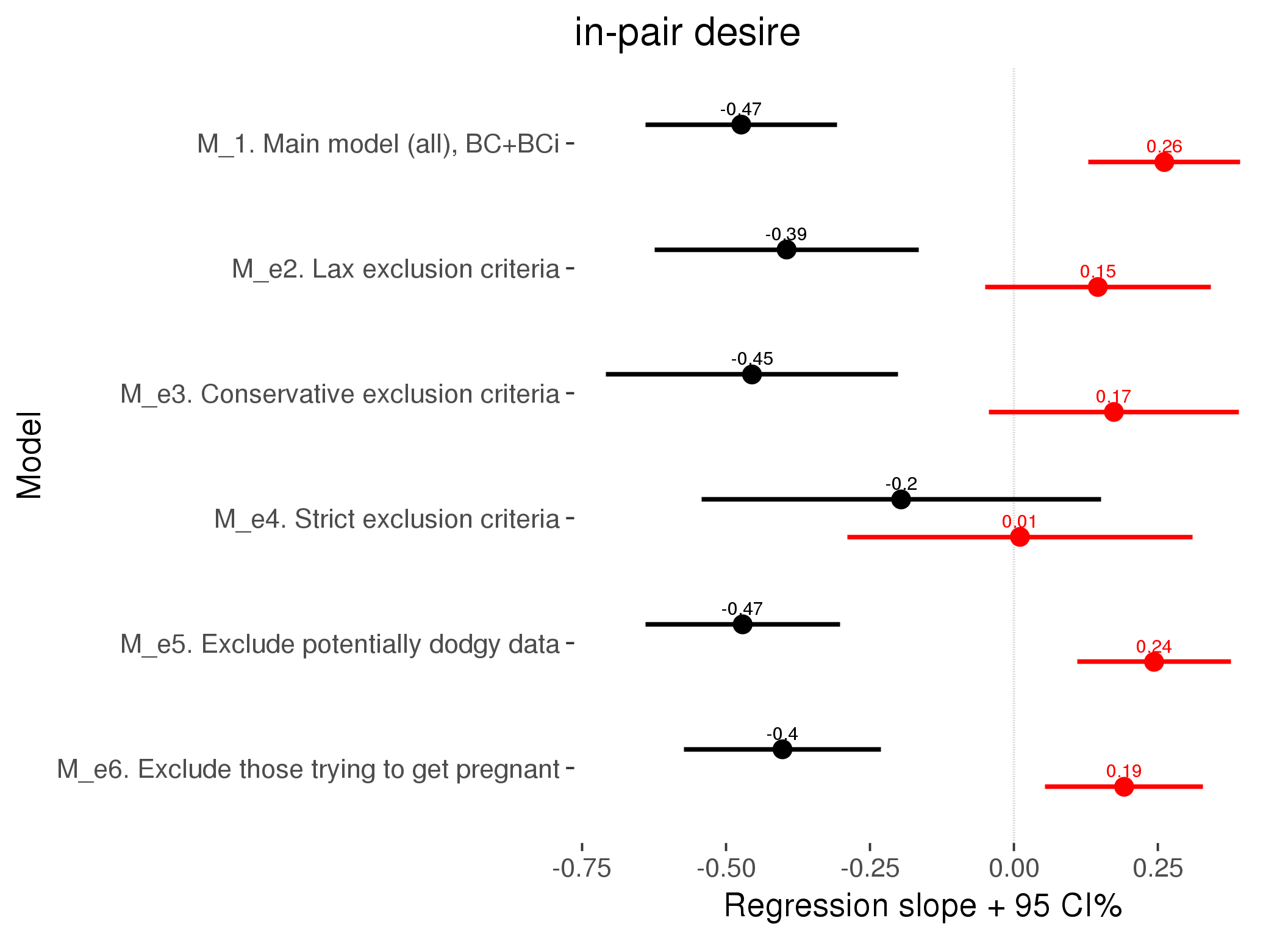
M_p: Predictors
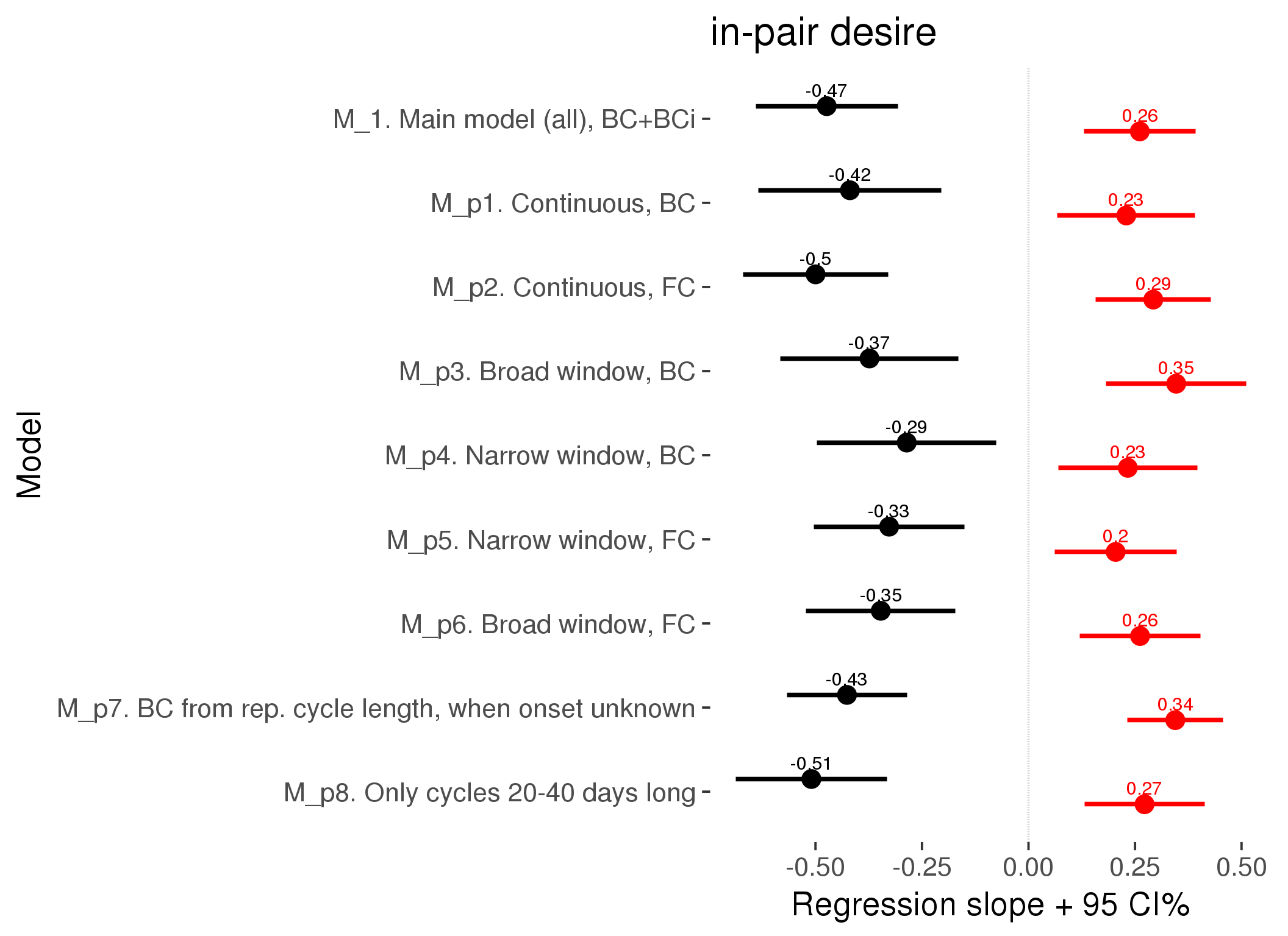
M_c: Covariates, controls, autocorrelation
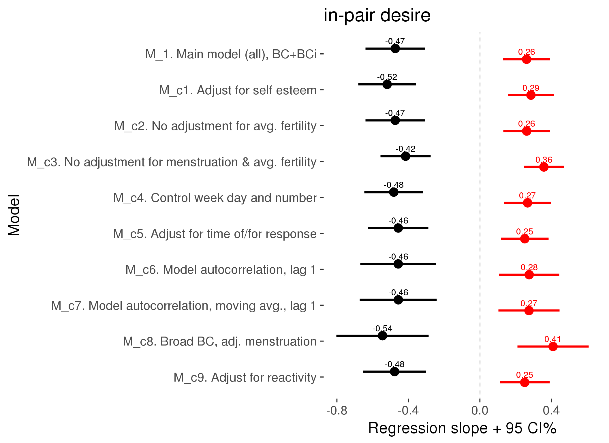
Linear mixed model fit by REML ['lmerMod']
REML criterion at convergence: 75701
Scaled residuals:
Min 1Q Median 3Q Max
-3.528 -0.682 -0.034 0.656 3.727
Random effects:
Groups Name Variance Std.Dev.
person (Intercept) 0.744 0.862
Xr.2 s(days_filled_out):includedhorm_contra 0.213 0.462
Xr.1 s(days_filled_out):includedcycling 0.120 0.347
Xr.0 s(day_number):includedhorm_contra 0.195 0.441
Xr s(day_number):includedcycling 0.265 0.515
Residual 1.168 1.081
Number of obs: 24377, groups: person, 1054; Xr.2, 8; Xr.1, 8; Xr.0, 8; Xr, 8
Fixed effects:
Estimate Std. Error t value
X(Intercept) 3.433548 0.076433 44.9
Xincludedhorm_contra 0.288701 0.063161 4.6
Xmenstruationpre -0.069772 0.034500 -2.0
Xmenstruationyes -0.206265 0.033124 -6.2
Xfertile 0.250923 0.071046 3.5
Xfertile_mean 0.111169 0.348689 0.3
Xincludedhorm_contra:menstruationpre -0.000389 0.044253 0.0
Xincludedhorm_contra:menstruationyes 0.048506 0.043355 1.1
Xincludedhorm_contra:fertile -0.477230 0.089937 -5.3
Xs(day_number):includedcyclingFx1 0.193693 0.148884 1.3
Xs(day_number):includedhorm_contraFx1 0.496596 0.139077 3.6
Xs(days_filled_out):includedcyclingFx1 -0.161664 0.131656 -1.2
Xs(days_filled_out):includedhorm_contraFx1 -0.478781 0.141323 -3.4
Family: gaussian
Link function: identity
Formula:
in_pair_desire ~ included + menstruation + fertile + fertile_mean +
s(day_number, by = included) + s(days_filled_out, by = included) +
included:menstruation + included:fertile
Parametric coefficients:
Estimate Std. Error t value Pr(>|t|)
(Intercept) 3.433548 0.076433 44.92 < 2e-16 ***
includedhorm_contra 0.288701 0.063161 4.57 0.00000488126 ***
menstruationpre -0.069772 0.034500 -2.02 0.04315 *
menstruationyes -0.206265 0.033124 -6.23 0.00000000048 ***
fertile 0.250923 0.071046 3.53 0.00041 ***
fertile_mean 0.111169 0.348689 0.32 0.74986
includedhorm_contra:menstruationpre -0.000389 0.044253 -0.01 0.99298
includedhorm_contra:menstruationyes 0.048506 0.043355 1.12 0.26323
includedhorm_contra:fertile -0.477230 0.089937 -5.31 0.00000011288 ***
---
Signif. codes: 0 '***' 0.001 '**' 0.01 '*' 0.05 '.' 0.1 ' ' 1
Approximate significance of smooth terms:
edf Ref.df F p-value
s(day_number):includedcycling 4.58 4.58 3.38 0.012 *
s(day_number):includedhorm_contra 4.49 4.49 9.10 0.0000000880 ***
s(days_filled_out):includedcycling 3.47 3.47 3.74 0.010 *
s(days_filled_out):includedhorm_contra 4.65 4.65 9.88 0.0000000098 ***
---
Signif. codes: 0 '***' 0.001 '**' 0.01 '*' 0.05 '.' 0.1 ' ' 1
R-sq.(adj) = 0.0073
lmer.REML = 75701 Scale est. = 1.1676 n = 24377
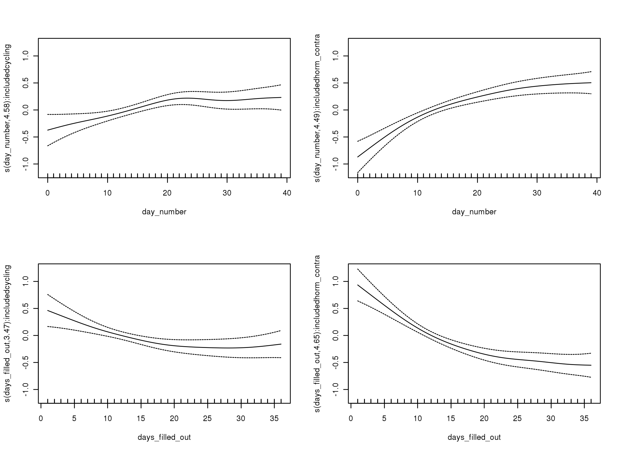
Linear mixed-effects model fit by REML
Data: diary
AIC BIC logLik
80351 80449 -40163
Random effects:
Formula: ~1 | person
(Intercept) Residual
StdDev: 0.8243 1.11
Correlation Structure: ARMA(1,0)
Formula: ~day_number | person
Parameter estimate(s):
Phi1
0.3693
Fixed effects: in_pair_desire ~ included * (menstruation + fertile) + fertile_mean
Value Std.Error DF t-value p-value
(Intercept) 3.468 0.0770 25620 45.03 0.0000
includedhorm_contra 0.288 0.0635 1051 4.53 0.0000
menstruationpre -0.051 0.0394 25620 -1.29 0.1979
menstruationyes -0.182 0.0367 25620 -4.95 0.0000
fertile 0.276 0.0858 25620 3.21 0.0013
fertile_mean 0.082 0.3546 1051 0.23 0.8169
includedhorm_contra:menstruationpre -0.005 0.0506 25620 -0.10 0.9188
includedhorm_contra:menstruationyes 0.062 0.0477 25620 1.30 0.1932
includedhorm_contra:fertile -0.457 0.1084 25620 -4.21 0.0000
Correlation:
(Intr) incld_ mnstrtnp mnstrtny fertil frtl_m inclddhrm_cntr:mnstrtnp
includedhorm_contra -0.477
menstruationpre -0.195 0.243
menstruationyes -0.191 0.237 0.404
fertile -0.187 0.312 0.410 0.350
fertile_mean -0.767 -0.028 -0.007 -0.005 -0.089
includedhorm_contra:menstruationpre 0.159 -0.303 -0.778 -0.315 -0.318 -0.005
includedhorm_contra:menstruationyes 0.153 -0.289 -0.311 -0.769 -0.268 -0.004 0.389
includedhorm_contra:fertile 0.190 -0.394 -0.324 -0.276 -0.786 0.015 0.408
inclddhrm_cntr:mnstrtny
includedhorm_contra
menstruationpre
menstruationyes
fertile
fertile_mean
includedhorm_contra:menstruationpre
includedhorm_contra:menstruationyes
includedhorm_contra:fertile 0.343
Standardized Within-Group Residuals:
Min Q1 Med Q3 Max
-3.38144 -0.68695 -0.03729 0.65882 3.74443
Number of Observations: 26680
Number of Groups: 1054
Linear mixed-effects model fit by REML
Data: diary
AIC BIC logLik
80332 80438 -40153
Random effects:
Formula: ~1 | person
(Intercept) Residual
StdDev: 0.8207 1.112
Correlation Structure: ARMA(1,1)
Formula: ~day_number | person
Parameter estimate(s):
Phi1 Theta1
0.44522 -0.08788
Fixed effects: in_pair_desire ~ included * (menstruation + fertile) + fertile_mean
Value Std.Error DF t-value p-value
(Intercept) 3.468 0.0771 25620 44.99 0.0000
includedhorm_contra 0.288 0.0636 1051 4.53 0.0000
menstruationpre -0.048 0.0396 25620 -1.20 0.2297
menstruationyes -0.182 0.0369 25620 -4.94 0.0000
fertile 0.275 0.0869 25620 3.16 0.0016
fertile_mean 0.085 0.3550 1051 0.24 0.8104
includedhorm_contra:menstruationpre -0.008 0.0509 25620 -0.15 0.8799
includedhorm_contra:menstruationyes 0.061 0.0480 25620 1.27 0.2042
includedhorm_contra:fertile -0.456 0.1098 25620 -4.15 0.0000
Correlation:
(Intr) incld_ mnstrtnp mnstrtny fertil frtl_m inclddhrm_cntr:mnstrtnp
includedhorm_contra -0.477
menstruationpre -0.195 0.243
menstruationyes -0.192 0.238 0.407
fertile -0.188 0.314 0.401 0.347
fertile_mean -0.767 -0.028 -0.006 -0.005 -0.090
includedhorm_contra:menstruationpre 0.159 -0.303 -0.778 -0.317 -0.311 -0.005
includedhorm_contra:menstruationyes 0.154 -0.291 -0.313 -0.769 -0.266 -0.004 0.393
includedhorm_contra:fertile 0.191 -0.397 -0.317 -0.274 -0.786 0.015 0.400
inclddhrm_cntr:mnstrtny
includedhorm_contra
menstruationpre
menstruationyes
fertile
fertile_mean
includedhorm_contra:menstruationpre
includedhorm_contra:menstruationyes
includedhorm_contra:fertile 0.340
Standardized Within-Group Residuals:
Min Q1 Med Q3 Max
-3.37254 -0.68777 -0.03708 0.66182 3.72189
Number of Observations: 26680
Number of Groups: 1054
M_d: Other designs
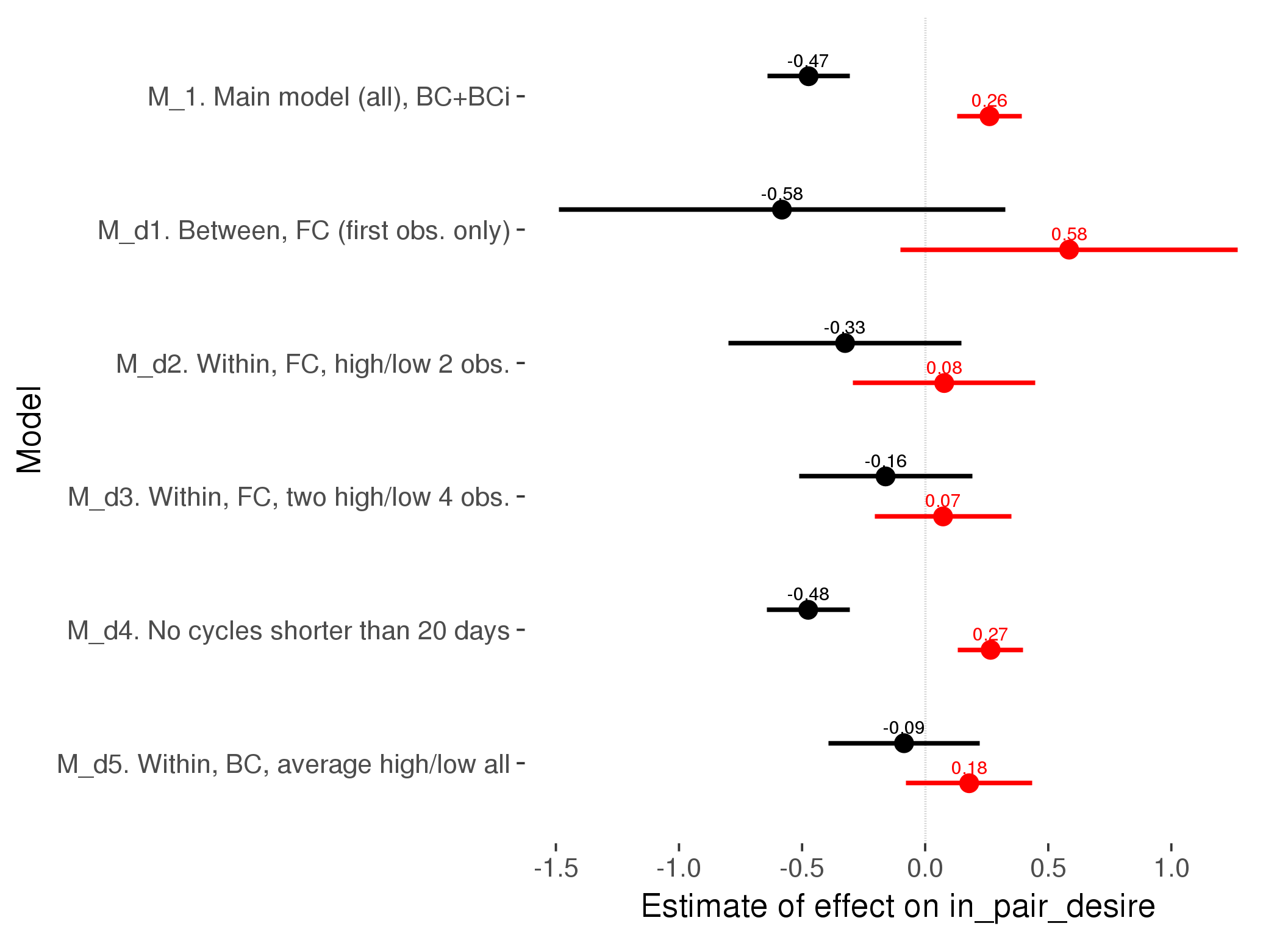
M_m1: Moderation by contraceptive method
Based on the sample with lax exclusion criteria. Users who used any hormonal contraception are classified as hormonal, users who use any awareness-based methods (counting, temperature-based) are classified as ‘fertility-awareness’, women who don’t fall into the before groups and use condoms, pessars, coitus interruptus etc. are classified as ‘barrie or abstinence’. Women who don’t use contraception or use other methods such as sterilisation are excluded from this analysis.
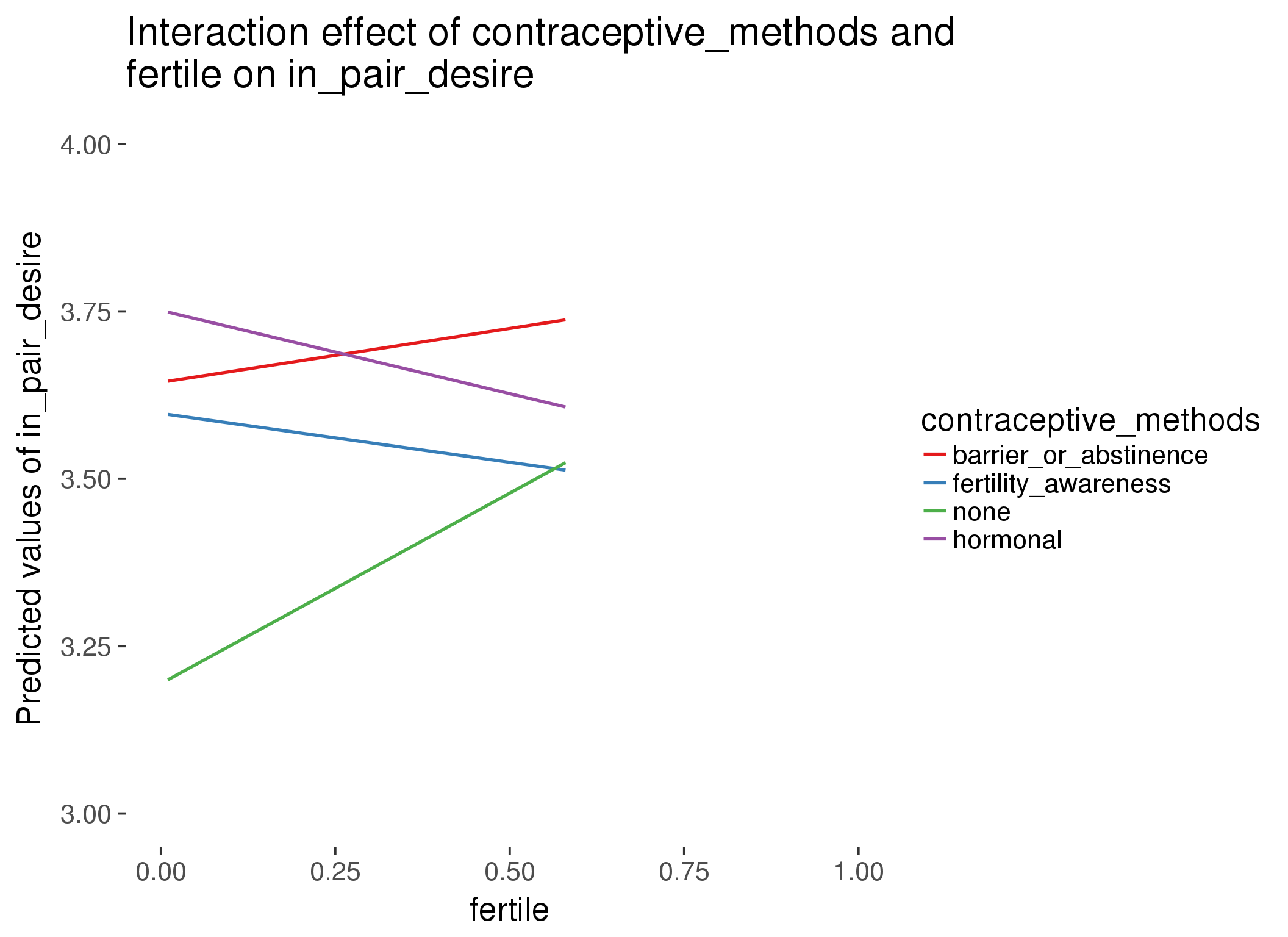
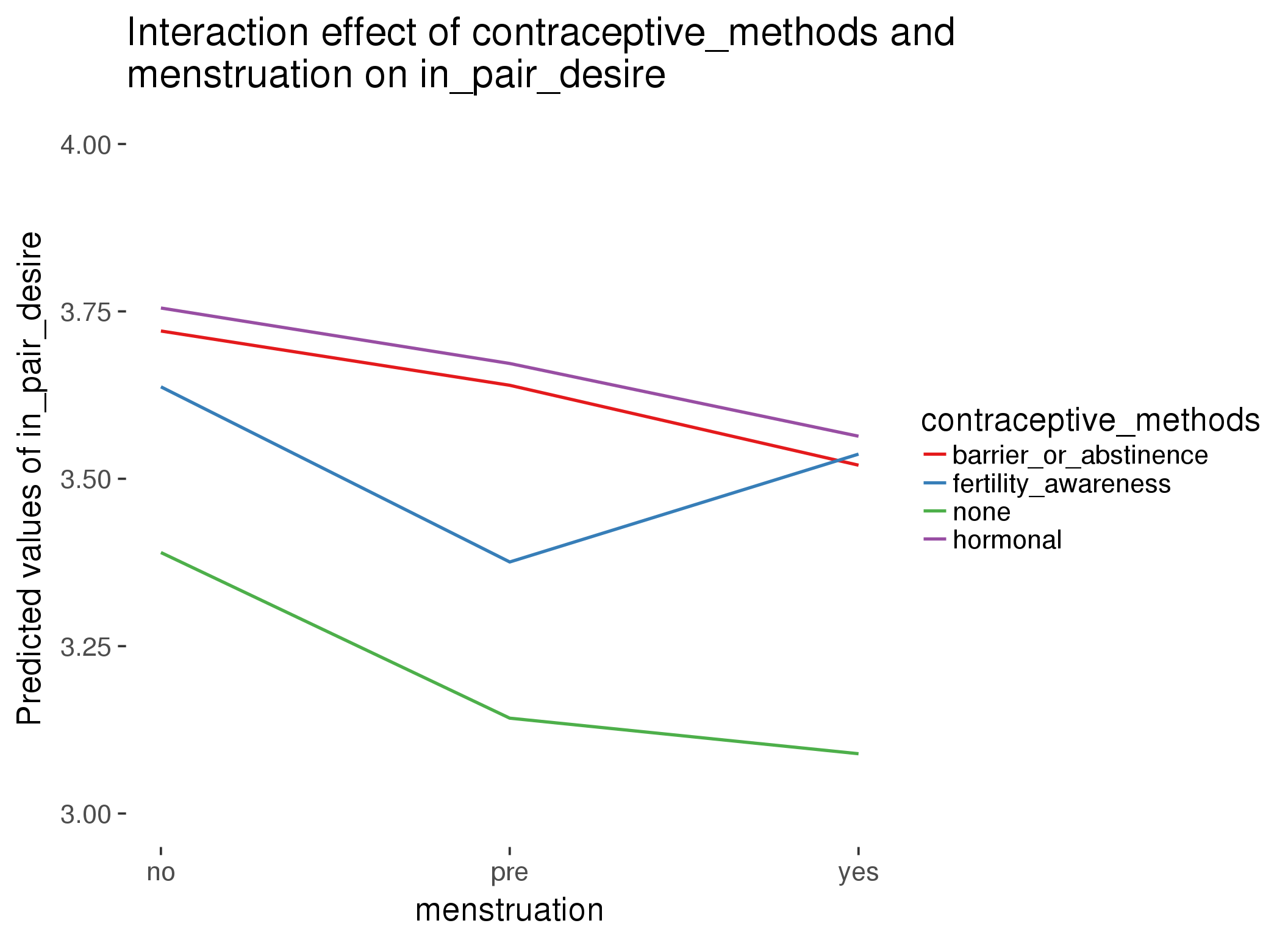
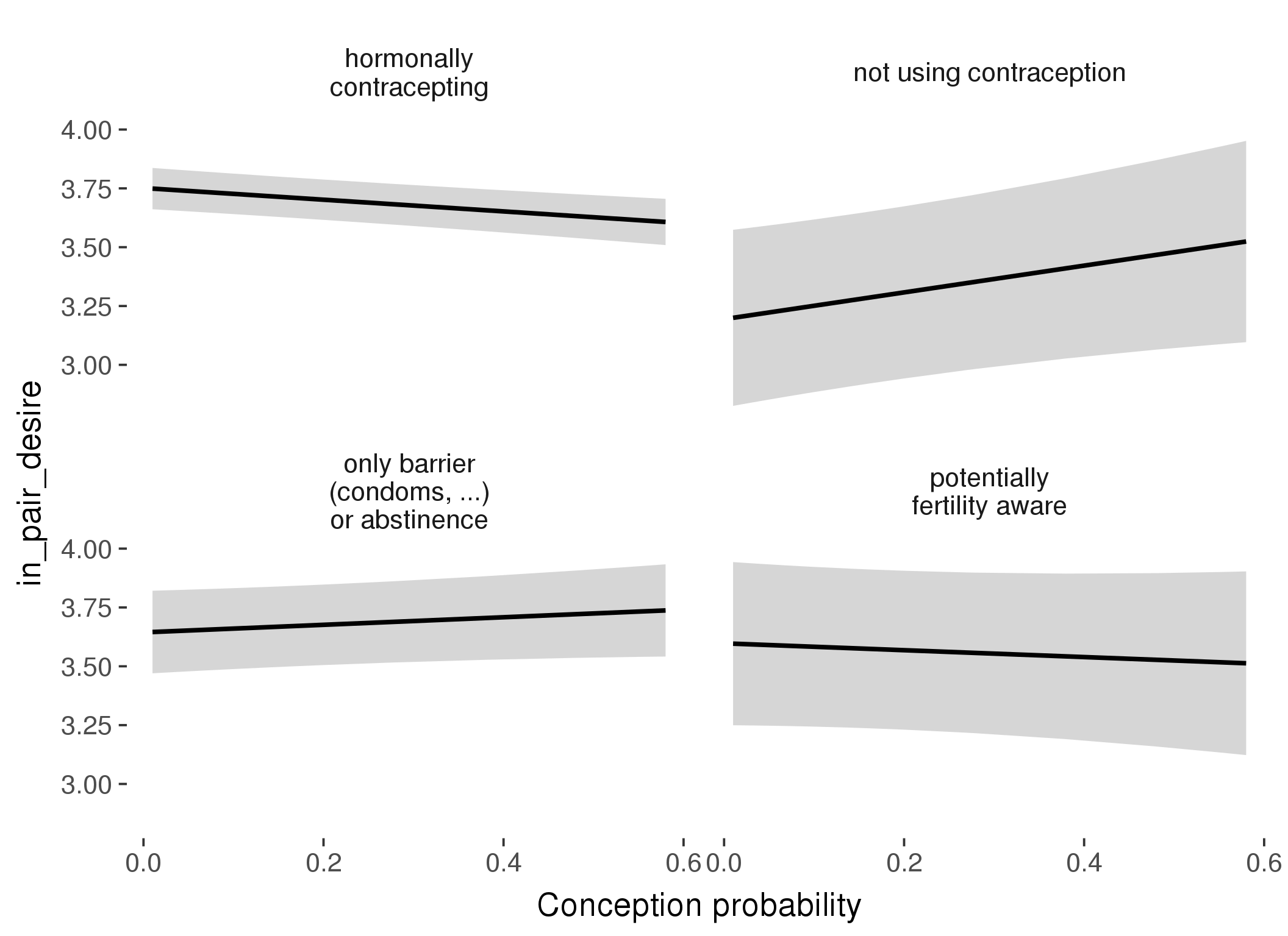
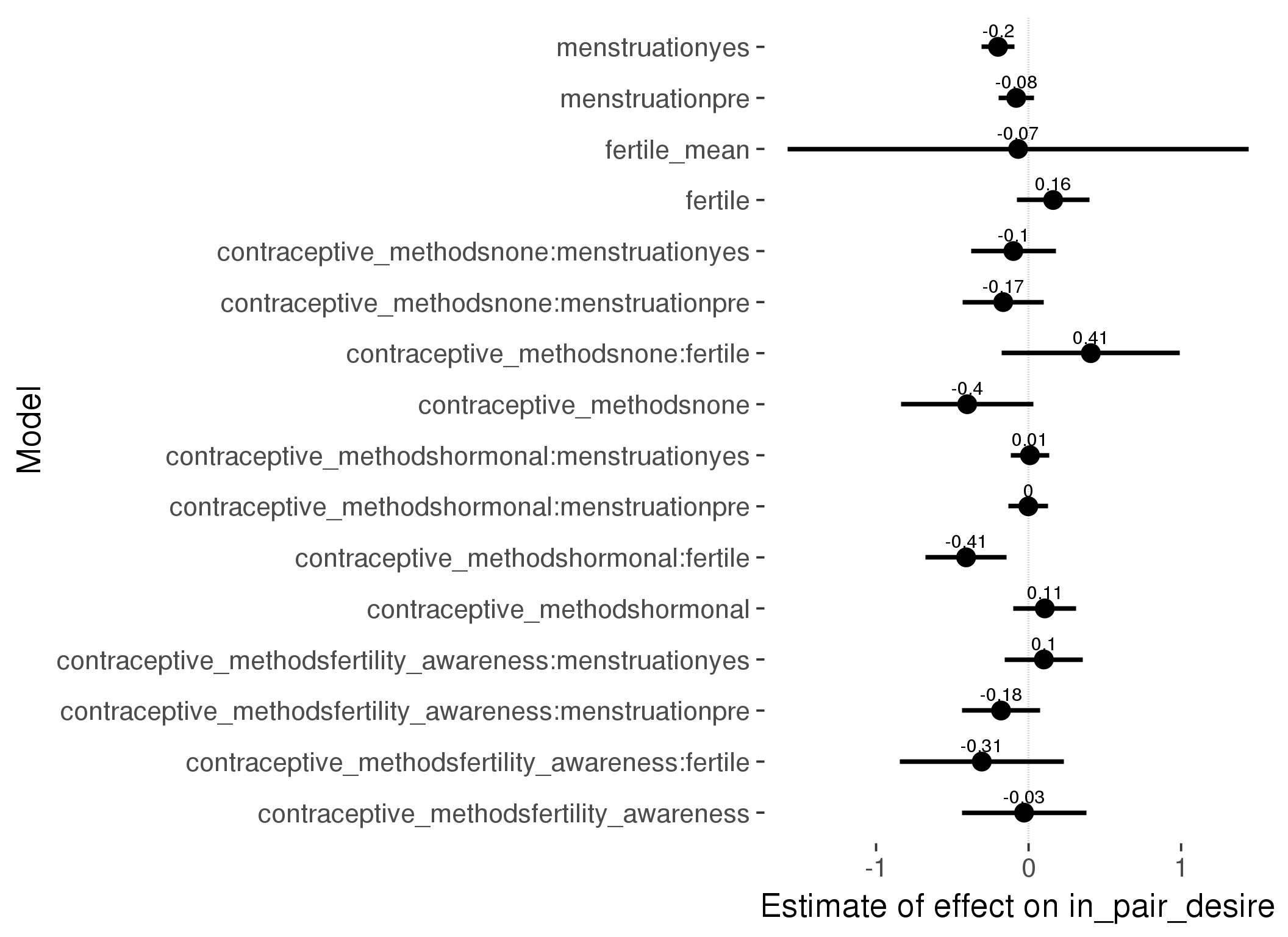
Linear mixed model fit by REML ['lmerMod']
Formula: in_pair_desire ~ fertile_mean + (1 | person) + contraceptive_methods +
fertile + menstruation + fertile:contraceptive_methods + menstruation:contraceptive_methods
Data: diary
Subset: !is.na(included_lax) & contraceptive_method != "other"
REML criterion at convergence: 52683
Scaled residuals:
Min 1Q Median 3Q Max
-3.489 -0.682 -0.039 0.670 3.439
Random effects:
Groups Name Variance Std.Dev.
person (Intercept) 0.674 0.821
Residual 1.179 1.086
Number of obs: 17026, groups: person, 513
Fixed effects:
Estimate Std. Error t value
(Intercept) 3.70449 0.15897 23.30
fertile_mean -0.06860 0.77147 -0.09
contraceptive_methodsfertility_awareness -0.02951 0.20787 -0.14
contraceptive_methodsnone -0.40242 0.22038 -1.83
contraceptive_methodshormonal 0.10620 0.10475 1.01
fertile 0.16094 0.12113 1.33
menstruationpre -0.08107 0.05851 -1.39
menstruationyes -0.20042 0.05588 -3.59
contraceptive_methodsfertility_awareness:fertile -0.30697 0.27510 -1.12
contraceptive_methodsnone:fertile 0.40800 0.29783 1.37
contraceptive_methodshormonal:fertile -0.40963 0.13531 -3.03
contraceptive_methodsfertility_awareness:menstruationpre -0.18053 0.12961 -1.39
contraceptive_methodsnone:menstruationpre -0.16633 0.13549 -1.23
contraceptive_methodshormonal:menstruationpre -0.00178 0.06590 -0.03
contraceptive_methodsfertility_awareness:menstruationyes 0.09994 0.13025 0.77
contraceptive_methodsnone:menstruationyes -0.10010 0.14168 -0.71
contraceptive_methodshormonal:menstruationyes 0.00895 0.06373 0.14
refitting model(s) with ML (instead of REML)
| Df | AIC | BIC | logLik | deviance | Chisq | Chi Df | Pr(>Chisq) | |
|---|---|---|---|---|---|---|---|---|
| add_main | 13 | 52675 | 52775 | -26324 | 52649 | NA | NA | NA |
| by_method | 19 | 52674 | 52821 | -26318 | 52636 | 13.13 | 6 | 0.04103 |
M_m2: Moderation by participant age
model %>%
test_moderator("age_group", diary, xlevels = 5)refitting model(s) with ML (instead of REML)
| Df | AIC | BIC | logLik | deviance | Chisq | Chi Df | Pr(>Chisq) | |
|---|---|---|---|---|---|---|---|---|
| with_main | 19 | 83064 | 83220 | -41513 | 83026 | NA | NA | NA |
| with_mod | 27 | 83057 | 83278 | -41502 | 83003 | 22.8 | 8 | 0.003634 |
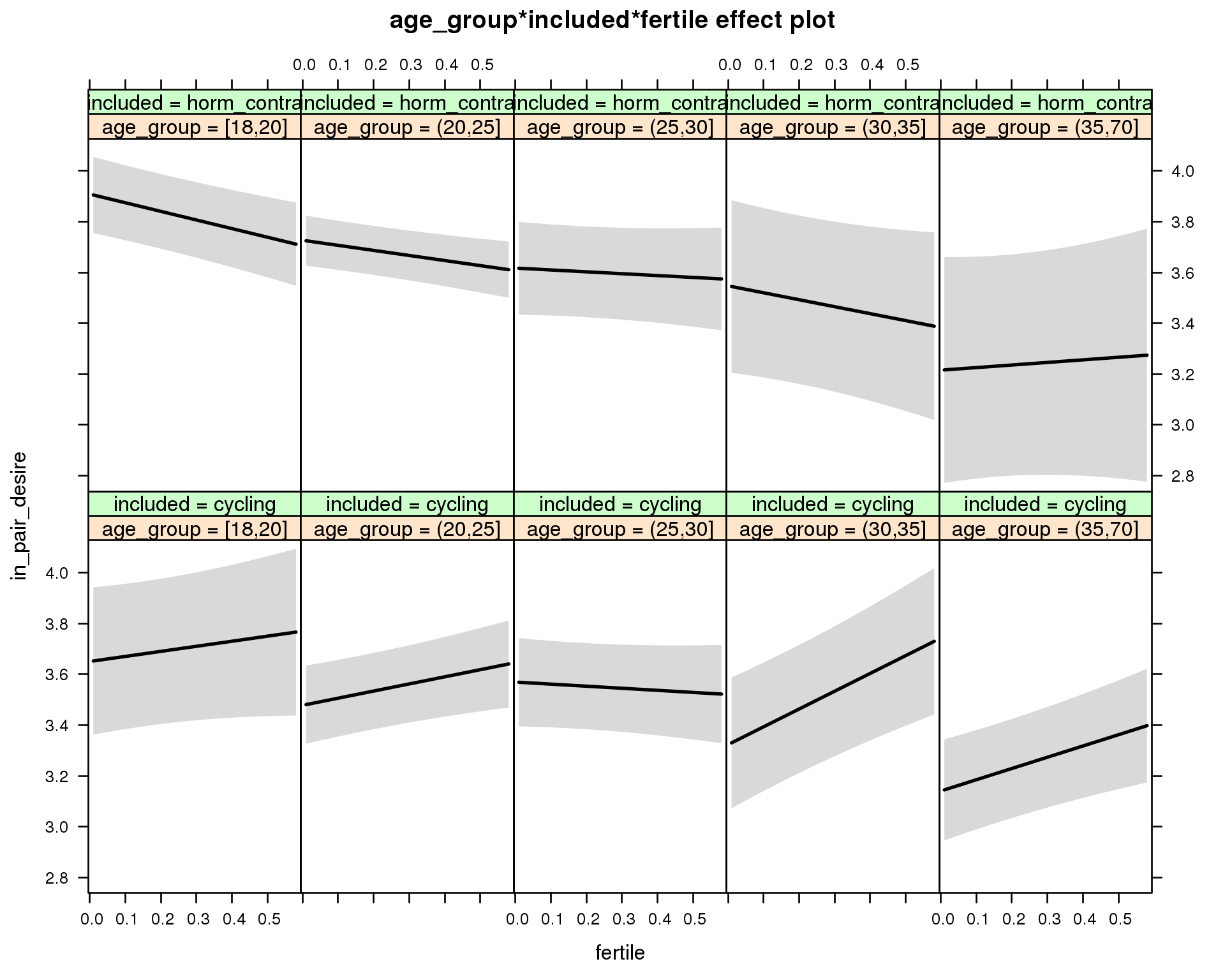
Linear mixed model fit by REML ['lmerMod']
Formula: in_pair_desire ~ menstruation + fertile_mean + (1 | person) +
age_group + included + fertile + menstruation:included +
age_group:included + age_group:fertile + included:fertile + age_group:included:fertile
Data: diary
REML criterion at convergence: 83073
Scaled residuals:
Min 1Q Median 3Q Max
-3.476 -0.678 -0.028 0.668 3.800
Random effects:
Groups Name Variance Std.Dev.
person (Intercept) 0.727 0.853
Residual 1.188 1.090
Number of obs: 26680, groups: person, 1054
Fixed effects:
Estimate Std. Error t value
(Intercept) 3.69249 0.15697 23.52
menstruationpre -0.06926 0.03327 -2.08
menstruationyes -0.19202 0.03136 -6.12
fertile_mean 0.02076 0.34699 0.06
age_group(20,25] -0.17249 0.16779 -1.03
age_group(25,30] -0.08092 0.17272 -0.47
age_group(30,35] -0.32733 0.19817 -1.65
age_group(35,70] -0.50998 0.17947 -2.84
includedhorm_contra 0.25205 0.16816 1.50
fertile 0.19954 0.19194 1.04
menstruationpre:includedhorm_contra -0.00329 0.04271 -0.08
menstruationyes:includedhorm_contra 0.04007 0.04111 0.97
age_group(20,25]:includedhorm_contra -0.00921 0.19130 -0.05
age_group(25,30]:includedhorm_contra -0.21025 0.21076 -1.00
age_group(30,35]:includedhorm_contra -0.03372 0.27432 -0.12
age_group(35,70]:includedhorm_contra -0.18323 0.29990 -0.61
age_group(20,25]:fertile 0.08104 0.21261 0.38
age_group(25,30]:fertile -0.28129 0.21915 -1.28
age_group(30,35]:fertile 0.50175 0.25382 1.98
age_group(35,70]:fertile 0.24387 0.22906 1.06
includedhorm_contra:fertile -0.53899 0.21289 -2.53
age_group(20,25]:includedhorm_contra:fertile 0.05880 0.23817 0.25
age_group(25,30]:includedhorm_contra:fertile 0.54708 0.26392 2.07
age_group(30,35]:includedhorm_contra:fertile -0.43643 0.34061 -1.28
age_group(35,70]:includedhorm_contra:fertile 0.19718 0.38702 0.51
M_m3: Moderation by weekend
model %>%
test_moderator("weekend", diary, xlevels = 2) refitting model(s) with ML (instead of REML)
| Df | AIC | BIC | logLik | deviance | Chisq | Chi Df | Pr(>Chisq) | |
|---|---|---|---|---|---|---|---|---|
| with_main | 13 | 82729 | 82836 | -41352 | 82703 | NA | NA | NA |
| with_mod | 15 | 82731 | 82854 | -41351 | 82701 | 1.82 | 2 | 0.4025 |
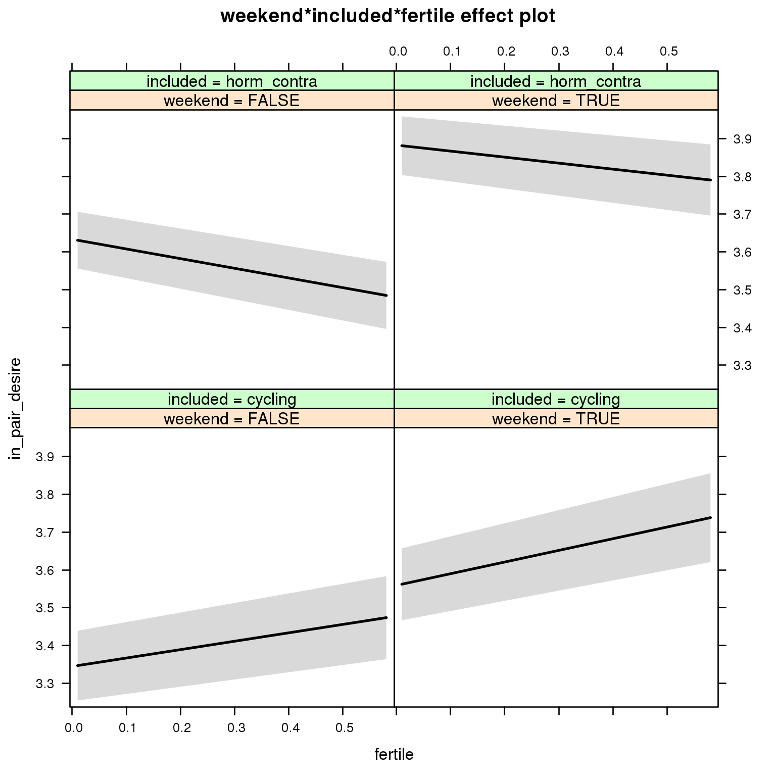
Linear mixed model fit by REML ['lmerMod']
Formula: in_pair_desire ~ menstruation + fertile_mean + (1 | person) +
weekend + included + fertile + menstruation:included + weekend:included +
weekend:fertile + included:fertile + weekend:included:fertile
Data: diary
REML criterion at convergence: 82758
Scaled residuals:
Min 1Q Median 3Q Max
-3.596 -0.673 -0.026 0.662 3.891
Random effects:
Groups Name Variance Std.Dev.
person (Intercept) 0.737 0.859
Residual 1.173 1.083
Number of obs: 26680, groups: person, 1054
Fixed effects:
Estimate Std. Error t value
(Intercept) 3.38146 0.07644 44.2
menstruationpre -0.06759 0.03305 -2.0
menstruationyes -0.18913 0.03114 -6.1
fertile_mean 0.04679 0.34669 0.1
weekendTRUE 0.21458 0.02881 7.4
includedhorm_contra 0.28222 0.06364 4.4
fertile 0.22267 0.08114 2.7
menstruationpre:includedhorm_contra -0.00489 0.04243 -0.1
menstruationyes:includedhorm_contra 0.04235 0.04083 1.0
weekendTRUE:includedhorm_contra 0.03480 0.03708 0.9
weekendTRUE:fertile 0.08652 0.11173 0.8
includedhorm_contra:fertile -0.47909 0.10309 -4.6
weekendTRUE:includedhorm_contra:fertile 0.01048 0.14211 0.1
M_m4: Moderation by weekday
model %>%
test_moderator("weekday", diary, xlevels = 7)refitting model(s) with ML (instead of REML)
| Df | AIC | BIC | logLik | deviance | Chisq | Chi Df | Pr(>Chisq) | |
|---|---|---|---|---|---|---|---|---|
| with_main | 23 | 82534 | 82723 | -41244 | 82488 | NA | NA | NA |
| with_mod | 35 | 82539 | 82826 | -41235 | 82469 | 19.32 | 12 | 0.08108 |
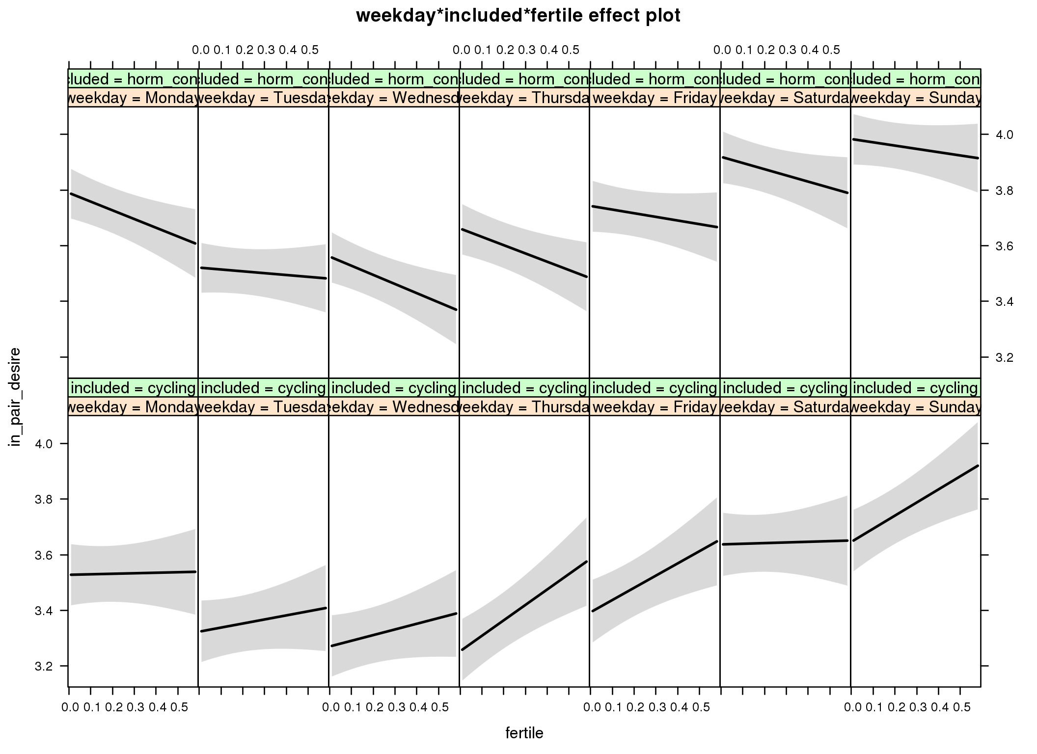
Linear mixed model fit by REML ['lmerMod']
Formula: in_pair_desire ~ menstruation + fertile_mean + (1 | person) +
weekday + included + fertile + menstruation:included + weekday:included +
weekday:fertile + included:fertile + weekday:included:fertile
Data: diary
REML criterion at convergence: 82594
Scaled residuals:
Min 1Q Median 3Q Max
-3.598 -0.669 -0.021 0.662 3.943
Random effects:
Groups Name Variance Std.Dev.
person (Intercept) 0.739 0.86
Residual 1.163 1.08
Number of obs: 26680, groups: person, 1054
Fixed effects:
Estimate Std. Error t value
(Intercept) 3.56902 0.08261 43.2
menstruationpre -0.06795 0.03292 -2.1
menstruationyes -0.19015 0.03101 -6.1
fertile_mean 0.02397 0.34672 0.1
weekdayTuesday -0.20447 0.05134 -4.0
weekdayWednesday -0.25772 0.05125 -5.0
weekdayThursday -0.27499 0.05184 -5.3
weekdayFriday -0.13476 0.05271 -2.6
weekdaySaturday 0.10928 0.05324 2.1
weekdaySunday 0.11856 0.05145 2.3
includedhorm_contra 0.25455 0.07517 3.4
fertile 0.01847 0.14459 0.1
menstruationpre:includedhorm_contra -0.00272 0.04226 -0.1
menstruationyes:includedhorm_contra 0.04529 0.04066 1.1
weekdayTuesday:includedhorm_contra -0.06445 0.06596 -1.0
weekdayWednesday:includedhorm_contra 0.02847 0.06617 0.4
weekdayThursday:includedhorm_contra 0.14669 0.06681 2.2
weekdayFriday:includedhorm_contra 0.08778 0.06772 1.3
weekdaySaturday:includedhorm_contra 0.02055 0.06851 0.3
weekdaySunday:includedhorm_contra 0.07517 0.06641 1.1
weekdayTuesday:fertile 0.12784 0.19904 0.6
weekdayWednesday:fertile 0.18574 0.19997 0.9
weekdayThursday:fertile 0.53738 0.20283 2.6
weekdayFriday:fertile 0.42100 0.20319 2.1
weekdaySaturday:fertile 0.00518 0.20589 0.0
weekdaySunday:fertile 0.45332 0.20009 2.3
includedhorm_contra:fertile -0.33181 0.18495 -1.8
weekdayTuesday:includedhorm_contra:fertile 0.11935 0.25404 0.5
weekdayWednesday:includedhorm_contra:fertile -0.20132 0.25605 -0.8
weekdayThursday:includedhorm_contra:fertile -0.52273 0.25815 -2.0
weekdayFriday:includedhorm_contra:fertile -0.23864 0.25892 -0.9
weekdaySaturday:includedhorm_contra:fertile 0.08497 0.26265 0.3
weekdaySunday:includedhorm_contra:fertile -0.25817 0.25559 -1.0
M_m5: Moderation by exclusion threshold
model %>%
test_moderator("included_levels", diary, xlevels = 4)refitting model(s) with ML (instead of REML)
| Df | AIC | BIC | logLik | deviance | Chisq | Chi Df | Pr(>Chisq) | |
|---|---|---|---|---|---|---|---|---|
| with_main | 17 | 83076 | 83215 | -41521 | 83042 | NA | NA | NA |
| with_mod | 23 | 83084 | 83272 | -41519 | 83038 | 3.696 | 6 | 0.7178 |
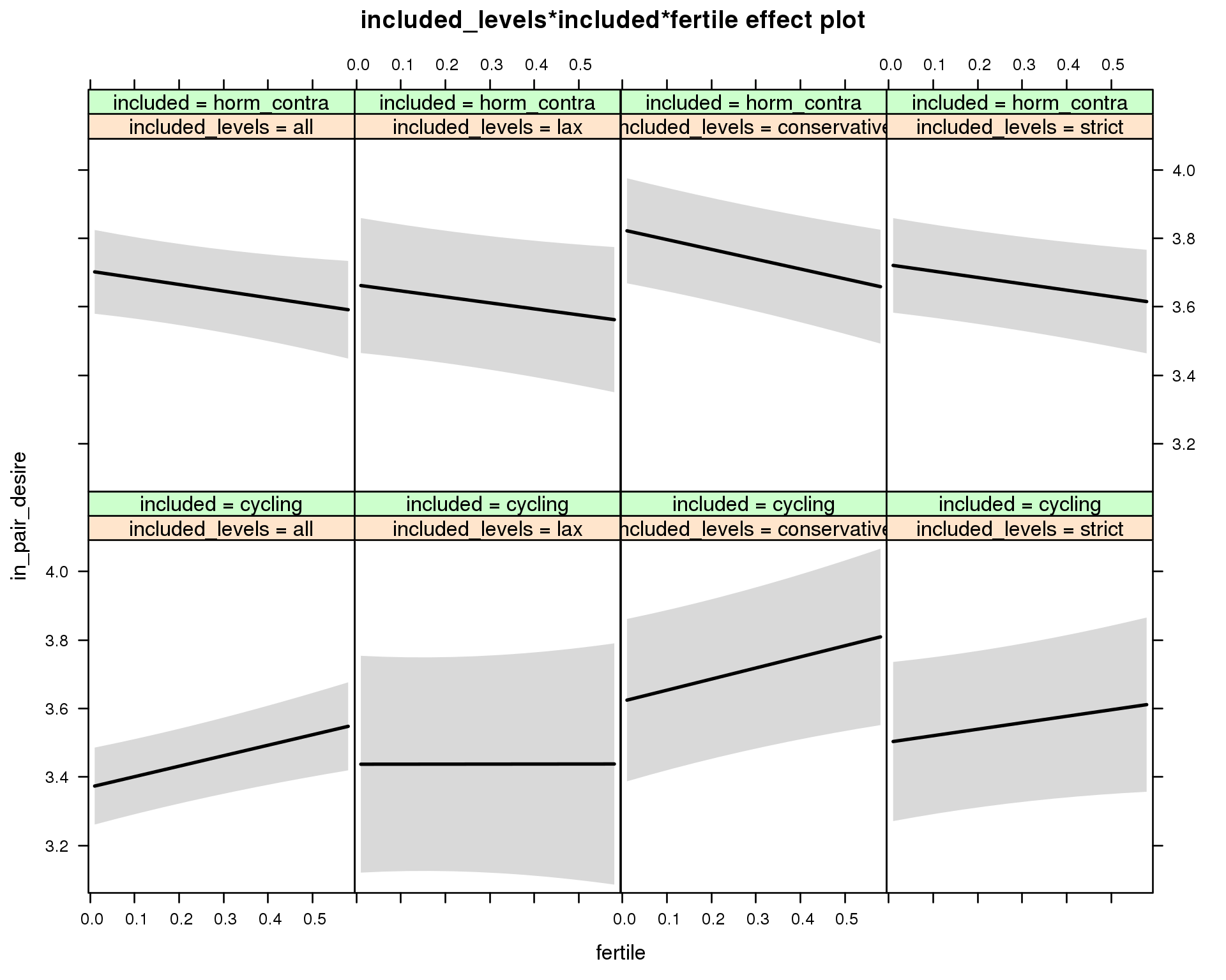
Linear mixed model fit by REML ['lmerMod']
Formula: in_pair_desire ~ menstruation + fertile_mean + (1 | person) +
included_levels + included + fertile + menstruation:included +
included_levels:included + included_levels:fertile + included:fertile +
included_levels:included:fertile
Data: diary
REML criterion at convergence: 83104
Scaled residuals:
Min 1Q Median 3Q Max
-3.488 -0.677 -0.031 0.667 3.764
Random effects:
Groups Name Variance Std.Dev.
person (Intercept) 0.736 0.858
Residual 1.189 1.090
Number of obs: 26680, groups: person, 1054
Fixed effects:
Estimate Std. Error t value
(Intercept) 3.41458 0.08395 40.7
menstruationpre -0.06967 0.03330 -2.1
menstruationyes -0.18737 0.03136 -6.0
fertile_mean 0.00622 0.35042 0.0
included_levelslax 0.06678 0.17141 0.4
included_levelsconservative 0.25059 0.13379 1.9
included_levelsstrict 0.13118 0.13163 1.0
includedhorm_contra 0.32704 0.08666 3.8
fertile 0.30577 0.08487 3.6
menstruationpre:includedhorm_contra -0.00153 0.04277 0.0
menstruationyes:includedhorm_contra 0.03672 0.04115 0.9
included_levelslax:includedhorm_contra -0.10687 0.20872 -0.5
included_levelsconservative:includedhorm_contra -0.12982 0.16719 -0.8
included_levelsstrict:includedhorm_contra -0.11242 0.16185 -0.7
included_levelslax:fertile -0.30457 0.20730 -1.5
included_levelsconservative:fertile 0.01806 0.15481 0.1
included_levelsstrict:fertile -0.11705 0.15492 -0.8
includedhorm_contra:fertile -0.49956 0.12958 -3.9
included_levelslax:includedhorm_contra:fertile 0.32379 0.25294 1.3
included_levelsconservative:includedhorm_contra:fertile -0.11028 0.20128 -0.5
included_levelsstrict:includedhorm_contra:fertile 0.12578 0.19817 0.6
M_m6: Moderation by cycle length
model %>%
test_moderator("cycle_length_groups", diary, xlevels = 4)refitting model(s) with ML (instead of REML)
| Df | AIC | BIC | logLik | deviance | Chisq | Chi Df | Pr(>Chisq) | |
|---|---|---|---|---|---|---|---|---|
| with_main | 17 | 83070 | 83209 | -41518 | 83036 | NA | NA | NA |
| with_mod | 23 | 83076 | 83264 | -41515 | 83030 | 5.943 | 6 | 0.4296 |
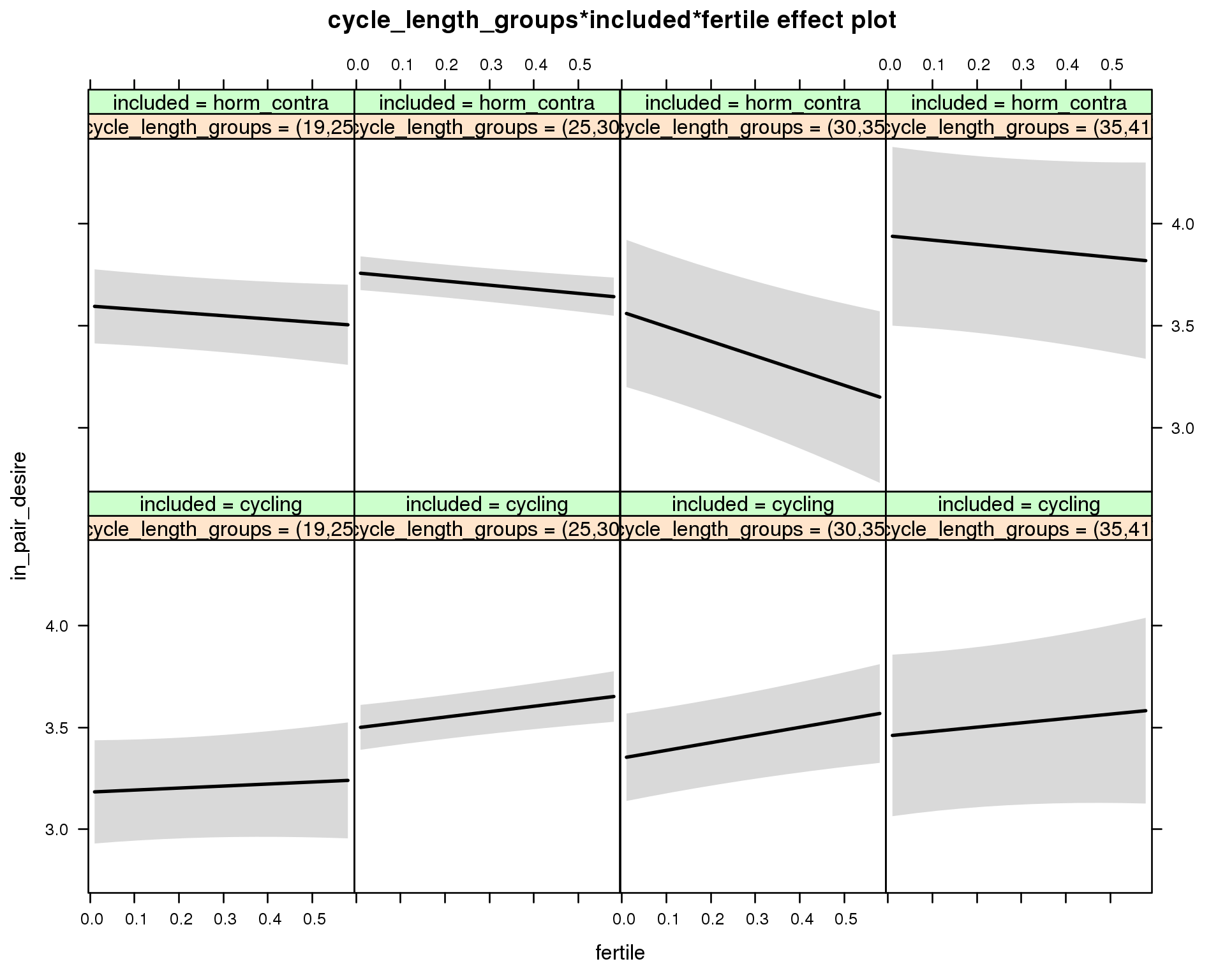
Linear mixed model fit by REML ['lmerMod']
Formula: in_pair_desire ~ menstruation + fertile_mean + (1 | person) +
cycle_length_groups + included + fertile + menstruation:included +
cycle_length_groups:included + cycle_length_groups:fertile +
included:fertile + cycle_length_groups:included:fertile
Data: diary
REML criterion at convergence: 83088
Scaled residuals:
Min 1Q Median 3Q Max
-3.484 -0.679 -0.030 0.665 3.797
Random effects:
Groups Name Variance Std.Dev.
person (Intercept) 0.732 0.855
Residual 1.189 1.090
Number of obs: 26680, groups: person, 1054
Fixed effects:
Estimate Std. Error t value
(Intercept) 3.2228 0.1439 22.40
menstruationpre -0.0664 0.0333 -1.99
menstruationyes -0.1834 0.0316 -5.81
fertile_mean 0.0213 0.3507 0.06
cycle_length_groups(25,30] 0.3151 0.1412 2.23
cycle_length_groups(30,35] 0.1673 0.1698 0.99
cycle_length_groups(35,41] 0.2760 0.2406 1.15
includedhorm_contra 0.4084 0.1605 2.54
fertile 0.0987 0.1772 0.56
menstruationpre:includedhorm_contra -0.0031 0.0428 -0.07
menstruationyes:includedhorm_contra 0.0339 0.0413 0.82
cycle_length_groups(25,30]:includedhorm_contra -0.1520 0.1742 -0.87
cycle_length_groups(30,35]:includedhorm_contra -0.1966 0.2672 -0.74
cycle_length_groups(35,41]:includedhorm_contra 0.0685 0.3412 0.20
cycle_length_groups(25,30]:fertile 0.1666 0.1901 0.88
cycle_length_groups(30,35]:fertile 0.2779 0.2251 1.23
cycle_length_groups(35,41]:fertile 0.1141 0.3180 0.36
includedhorm_contra:fertile -0.2571 0.2092 -1.23
cycle_length_groups(25,30]:includedhorm_contra:fertile -0.2100 0.2252 -0.93
cycle_length_groups(30,35]:includedhorm_contra:fertile -0.8393 0.3544 -2.37
cycle_length_groups(35,41]:includedhorm_contra:fertile -0.1653 0.4187 -0.39
M_m7: Moderation by certainty about menstruation parameters
model %>%
test_moderator("certainty_menstruation", diary)refitting model(s) with ML (instead of REML)
| Df | AIC | BIC | logLik | deviance | Chisq | Chi Df | Pr(>Chisq) | |
|---|---|---|---|---|---|---|---|---|
| with_main | 13 | 83069 | 83176 | -41522 | 83043 | NA | NA | NA |
| with_mod | 15 | 83062 | 83185 | -41516 | 83032 | 11.33 | 2 | 0.003466 |
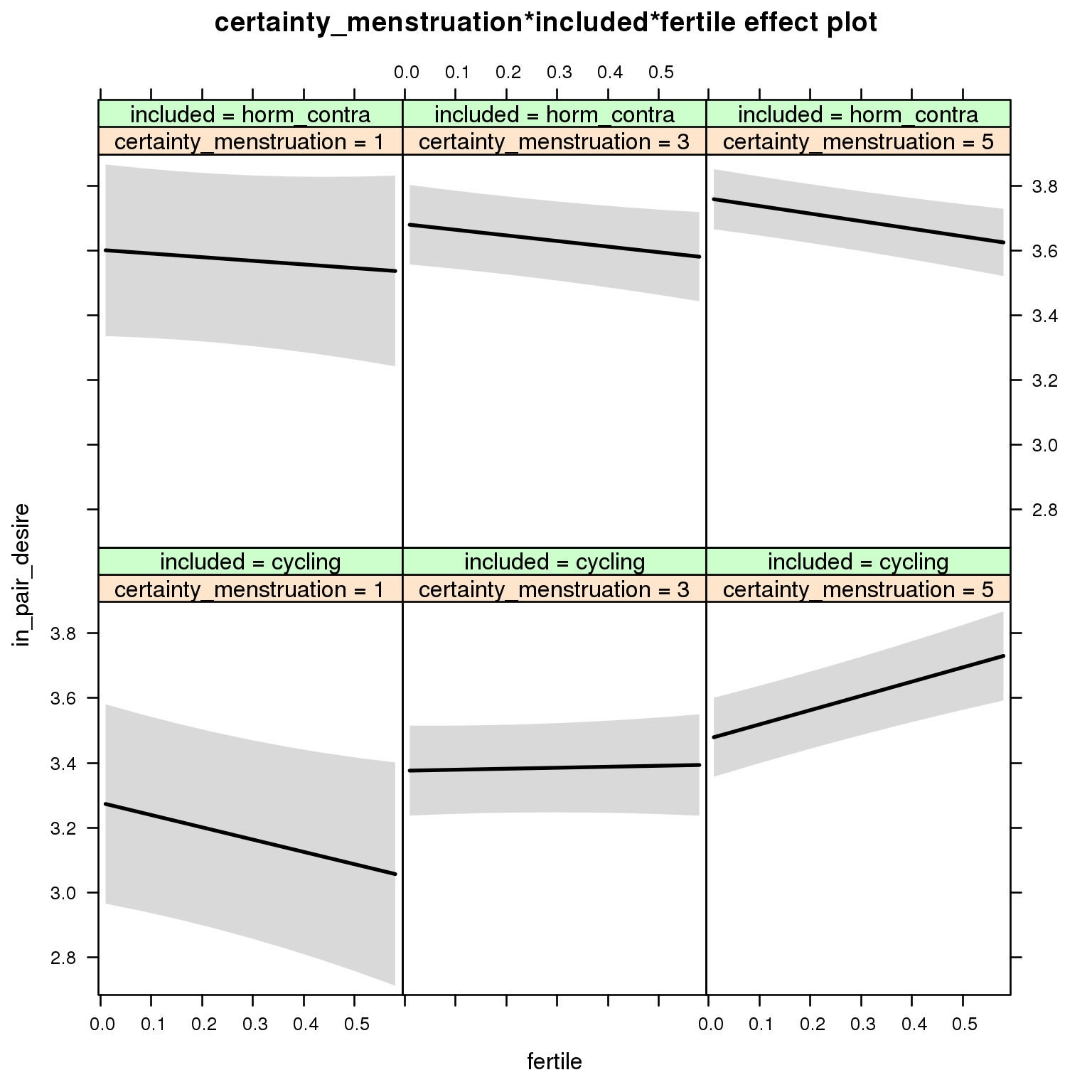
Linear mixed model fit by REML ['lmerMod']
Formula: in_pair_desire ~ menstruation + fertile_mean + (1 | person) +
certainty_menstruation + included + fertile + menstruation:included +
certainty_menstruation:included + certainty_menstruation:fertile +
included:fertile + certainty_menstruation:included:fertile
Data: diary
REML criterion at convergence: 83088
Scaled residuals:
Min 1Q Median 3Q Max
-3.483 -0.678 -0.032 0.668 3.822
Random effects:
Groups Name Variance Std.Dev.
person (Intercept) 0.734 0.857
Residual 1.188 1.090
Number of obs: 26680, groups: person, 1054
Fixed effects:
Estimate Std. Error t value
(Intercept) 3.26851 0.21152 15.45
menstruationpre -0.06397 0.03328 -1.92
menstruationyes -0.18188 0.03139 -5.79
fertile_mean 0.01146 0.34744 0.03
certainty_menstruation 0.04943 0.04820 1.03
includedhorm_contra 0.33000 0.26850 1.23
fertile -0.58428 0.26422 -2.21
menstruationpre:includedhorm_contra -0.00646 0.04272 -0.15
menstruationyes:includedhorm_contra 0.03152 0.04113 0.77
certainty_menstruation:includedhorm_contra -0.00974 0.06252 -0.16
certainty_menstruation:fertile 0.20489 0.06191 3.31
includedhorm_contra:fertile 0.50259 0.34343 1.46
certainty_menstruation:includedhorm_contra:fertile -0.23533 0.07938 -2.96
M_m8: Moderation by cycle regularity
model %>%
test_moderator("cycle_regularity", diary)refitting model(s) with ML (instead of REML)
| Df | AIC | BIC | logLik | deviance | Chisq | Chi Df | Pr(>Chisq) | |
|---|---|---|---|---|---|---|---|---|
| with_main | 15 | 83071 | 83194 | -41521 | 83041 | NA | NA | NA |
| with_mod | 19 | 83078 | 83233 | -41520 | 83040 | 1.613 | 4 | 0.8065 |
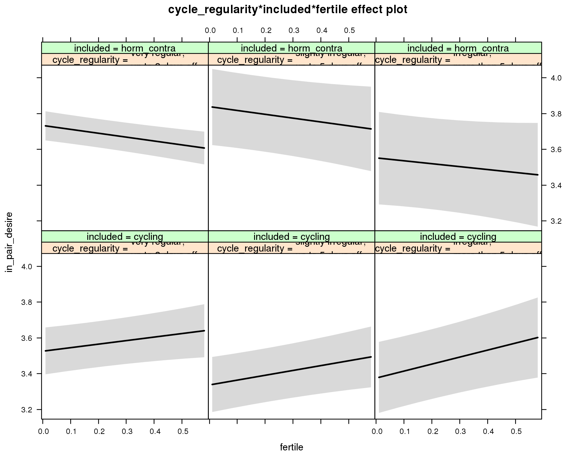
Linear mixed model fit by REML ['lmerMod']
Formula: in_pair_desire ~ menstruation + fertile_mean + (1 | person) +
cycle_regularity + included + fertile + menstruation:included +
cycle_regularity:included + cycle_regularity:fertile + included:fertile +
cycle_regularity:included:fertile
Data: diary
REML criterion at convergence: 83096
Scaled residuals:
Min 1Q Median 3Q Max
-3.479 -0.678 -0.031 0.665 3.787
Random effects:
Groups Name Variance Std.Dev.
person (Intercept) 0.735 0.857
Residual 1.189 1.090
Number of obs: 26680, groups: person, 1054
Fixed effects:
Estimate Std. Error t value
(Intercept) 3.56169 0.08914 40.0
menstruationpre -0.06934 0.03330 -2.1
menstruationyes -0.18866 0.03136 -6.0
fertile_mean 0.05098 0.34858 0.1
cycle_regularityslightly irregular,\nup to 5 days off -0.18858 0.10308 -1.8
cycle_regularityirregular,\nmore than 5 days off -0.15007 0.12132 -1.2
includedhorm_contra 0.20141 0.08108 2.5
fertile 0.19751 0.09298 2.1
menstruationpre:includedhorm_contra -0.00143 0.04274 0.0
menstruationyes:includedhorm_contra 0.03830 0.04112 0.9
cycle_regularityslightly irregular,\nup to 5 days off:includedhorm_contra 0.29381 0.15565 1.9
cycle_regularityirregular,\nmore than 5 days off:includedhorm_contra -0.03107 0.18413 -0.2
cycle_regularityslightly irregular,\nup to 5 days off:fertile 0.07277 0.12824 0.6
cycle_regularityirregular,\nmore than 5 days off:fertile 0.19319 0.15769 1.2
includedhorm_contra:fertile -0.41479 0.10893 -3.8
cycle_regularityslightly irregular,\nup to 5 days off:includedhorm_contra:fertile -0.06993 0.19043 -0.4
cycle_regularityirregular,\nmore than 5 days off:includedhorm_contra:fertile -0.13903 0.23540 -0.6
M_m9: Moderation by cohabitation status
model %>%
test_moderator("cohabitation", diary)refitting model(s) with ML (instead of REML)
| Df | AIC | BIC | logLik | deviance | Chisq | Chi Df | Pr(>Chisq) | |
|---|---|---|---|---|---|---|---|---|
| with_main | 15 | 83057 | 83180 | -41513 | 83027 | NA | NA | NA |
| with_mod | 19 | 83056 | 83211 | -41509 | 83018 | 9.394 | 4 | 0.05197 |
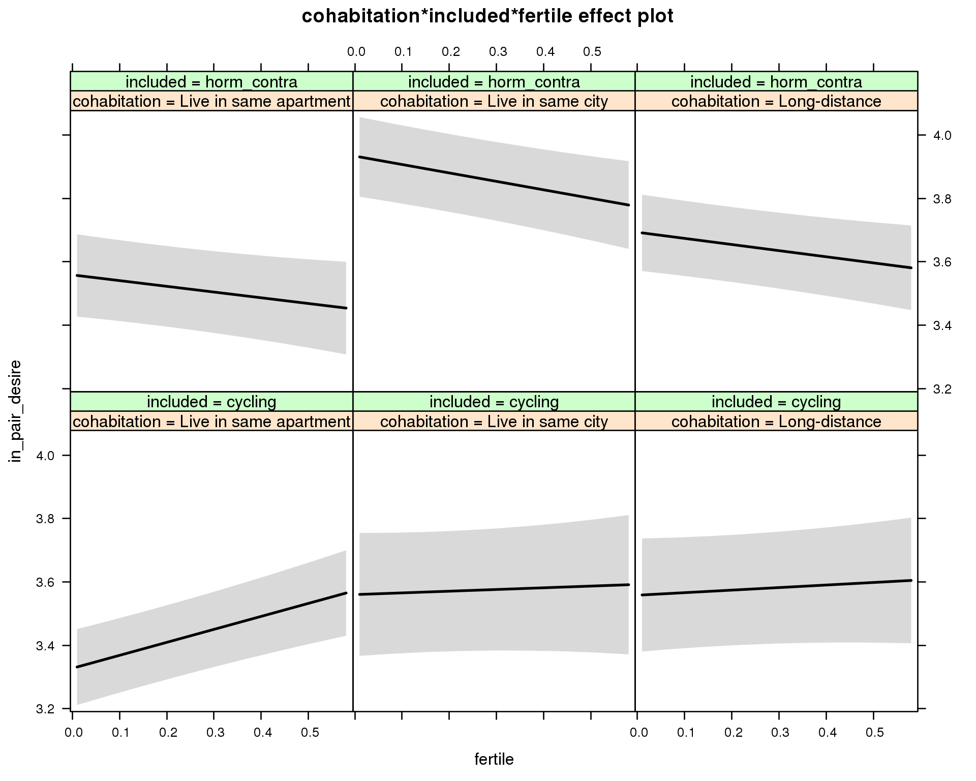
Linear mixed model fit by REML ['lmerMod']
Formula: in_pair_desire ~ menstruation + fertile_mean + (1 | person) +
cohabitation + included + fertile + menstruation:included +
cohabitation:included + cohabitation:fertile + included:fertile + cohabitation:included:fertile
Data: diary
REML criterion at convergence: 83078
Scaled residuals:
Min 1Q Median 3Q Max
-3.473 -0.679 -0.029 0.665 3.768
Random effects:
Groups Name Variance Std.Dev.
person (Intercept) 0.723 0.85
Residual 1.188 1.09
Number of obs: 26680, groups: person, 1054
Fixed effects:
Estimate Std. Error t value
(Intercept) 3.3728 0.0858 39.3
menstruationpre -0.0680 0.0333 -2.0
menstruationyes -0.1877 0.0314 -6.0
fertile_mean -0.0023 0.3456 0.0
cohabitationLive in same city 0.2326 0.1162 2.0
cohabitationLong-distance 0.2306 0.1095 2.1
includedhorm_contra 0.2255 0.0921 2.4
fertile 0.4097 0.0839 4.9
menstruationpre:includedhorm_contra -0.0039 0.0427 -0.1
menstruationyes:includedhorm_contra 0.0365 0.0411 0.9
cohabitationLive in same city:includedhorm_contra 0.1423 0.1485 1.0
cohabitationLong-distance:includedhorm_contra -0.0961 0.1421 -0.7
cohabitationLive in same city:fertile -0.3560 0.1533 -2.3
cohabitationLong-distance:fertile -0.3293 0.1381 -2.4
includedhorm_contra:fertile -0.5902 0.1226 -4.8
cohabitationLive in same city:includedhorm_contra:fertile 0.2702 0.1917 1.4
cohabitationLong-distance:includedhorm_contra:fertile 0.3165 0.1779 1.8
M_m10: Moderation by relationship status
model %>%
test_moderator("relationship_status_clean", diary)refitting model(s) with ML (instead of REML)
| Df | AIC | BIC | logLik | deviance | Chisq | Chi Df | Pr(>Chisq) | |
|---|---|---|---|---|---|---|---|---|
| with_main | 15 | 83058 | 83181 | -41514 | 83028 | NA | NA | NA |
| with_mod | 19 | 83062 | 83218 | -41512 | 83024 | 3.683 | 4 | 0.4505 |
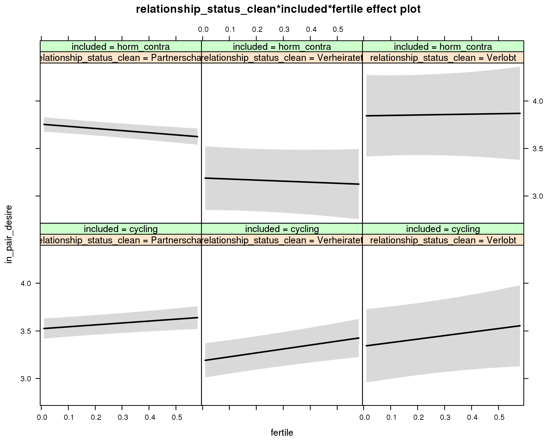
Linear mixed model fit by REML ['lmerMod']
Formula: in_pair_desire ~ menstruation + fertile_mean + (1 | person) +
relationship_status_clean + included + fertile + menstruation:included +
relationship_status_clean:included + relationship_status_clean:fertile +
included:fertile + relationship_status_clean:included:fertile
Data: diary
REML criterion at convergence: 83075
Scaled residuals:
Min 1Q Median 3Q Max
-3.478 -0.677 -0.030 0.667 3.786
Random effects:
Groups Name Variance Std.Dev.
person (Intercept) 0.723 0.85
Residual 1.189 1.09
Number of obs: 26680, groups: person, 1054
Fixed effects:
Estimate Std. Error t value
(Intercept) 3.56063 0.08033 44.3
menstruationpre -0.06783 0.03327 -2.0
menstruationyes -0.18765 0.03134 -6.0
fertile_mean 0.04050 0.34527 0.1
relationship_status_cleanVerheiratet -0.33663 0.10619 -3.2
relationship_status_cleanVerlobt -0.18312 0.20466 -0.9
includedhorm_contra 0.22621 0.06884 3.3
fertile 0.20076 0.07688 2.6
menstruationpre:includedhorm_contra -0.00339 0.04271 -0.1
menstruationyes:includedhorm_contra 0.03727 0.04109 0.9
relationship_status_cleanVerheiratet:includedhorm_contra -0.22870 0.20466 -1.1
relationship_status_cleanVerlobt:includedhorm_contra 0.27110 0.30221 0.9
relationship_status_cleanVerheiratet:fertile 0.21099 0.13534 1.6
relationship_status_cleanVerlobt:fertile 0.16829 0.25380 0.7
includedhorm_contra:fertile -0.42523 0.09371 -4.5
relationship_status_cleanVerheiratet:includedhorm_contra:fertile -0.09785 0.25486 -0.4
relationship_status_cleanVerlobt:includedhorm_contra:fertile 0.10122 0.39420 0.3
do_moderators(models$in_pair_desire, diary)Moderators
Partner’s physical attractiveness
Predicted fertile phase effect sizes (in red): biggest (EP desire, partner mate retention)/smallest (IP desire) when partner’s physical attractiveness is low.
model %>%
test_moderator("partner_attractiveness_physical", diary)refitting model(s) with ML (instead of REML)
| Df | AIC | BIC | logLik | deviance | Chisq | Chi Df | Pr(>Chisq) | |
|---|---|---|---|---|---|---|---|---|
| with_main | 13 | 82861 | 82967 | -41417 | 82835 | NA | NA | NA |
| with_mod | 15 | 82864 | 82986 | -41417 | 82834 | 1.362 | 2 | 0.506 |
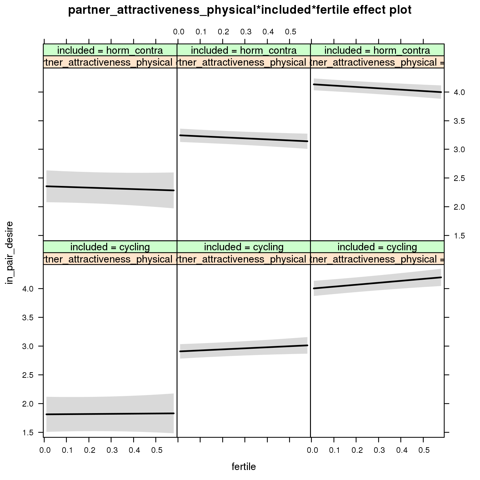
Linear mixed model fit by REML ['lmerMod']
Formula: in_pair_desire ~ menstruation + fertile_mean + (1 | person) +
partner_attractiveness_physical + included + fertile + menstruation:included +
partner_attractiveness_physical:included + partner_attractiveness_physical:fertile +
included:fertile + partner_attractiveness_physical:included:fertile
Data: diary
REML criterion at convergence: 82894
Scaled residuals:
Min 1Q Median 3Q Max
-3.476 -0.679 -0.029 0.667 3.765
Random effects:
Groups Name Variance Std.Dev.
person (Intercept) 0.593 0.77
Residual 1.188 1.09
Number of obs: 26680, groups: person, 1054
Fixed effects:
Estimate Std. Error t value
(Intercept) 1.31921 0.21259 6.21
menstruationpre -0.06928 0.03324 -2.08
menstruationyes -0.18954 0.03132 -6.05
fertile_mean -0.05585 0.32099 -0.17
partner_attractiveness_physical 0.27375 0.02544 10.76
includedhorm_contra 0.64365 0.27749 2.32
fertile -0.04778 0.29264 -0.16
menstruationpre:includedhorm_contra -0.00151 0.04267 -0.04
menstruationyes:includedhorm_contra 0.03834 0.04105 0.93
partner_attractiveness_physical:includedhorm_contra -0.05176 0.03381 -1.53
partner_attractiveness_physical:fertile 0.03850 0.03586 1.07
includedhorm_contra:fertile -0.05085 0.38722 -0.13
partner_attractiveness_physical:includedhorm_contra:fertile -0.05233 0.04682 -1.12
Partner’s short-term attractiveness
Predicted fertile phase effect sizes (in red): biggest (EP desire, partner mate retention)/smallest (IP desire) when partner’s short-term attractiveness is low.
model %>%
test_moderator("partner_attractiveness_shortterm", diary)refitting model(s) with ML (instead of REML)
| Df | AIC | BIC | logLik | deviance | Chisq | Chi Df | Pr(>Chisq) | |
|---|---|---|---|---|---|---|---|---|
| with_main | 13 | 82859 | 82965 | -41416 | 82833 | NA | NA | NA |
| with_mod | 15 | 82862 | 82985 | -41416 | 82832 | 0.3601 | 2 | 0.8352 |
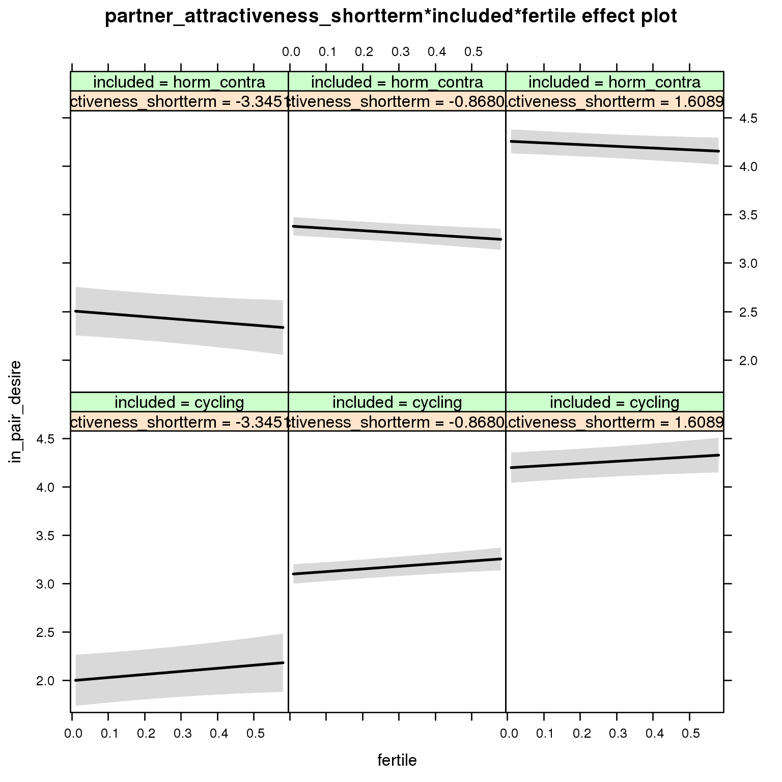
Linear mixed model fit by REML ['lmerMod']
Formula: in_pair_desire ~ menstruation + fertile_mean + (1 | person) +
partner_attractiveness_shortterm + included + fertile + menstruation:included +
partner_attractiveness_shortterm:included + partner_attractiveness_shortterm:fertile +
included:fertile + partner_attractiveness_shortterm:included:fertile
Data: diary
REML criterion at convergence: 82890
Scaled residuals:
Min 1Q Median 3Q Max
-3.489 -0.680 -0.031 0.665 3.738
Random effects:
Groups Name Variance Std.Dev.
person (Intercept) 0.589 0.768
Residual 1.188 1.090
Number of obs: 26680, groups: person, 1054
Fixed effects:
Estimate Std. Error t value
(Intercept) 3.53611 0.06974 50.7
menstruationpre -0.06853 0.03324 -2.1
menstruationyes -0.19000 0.03132 -6.1
fertile_mean -0.04066 0.32029 -0.1
partner_attractiveness_shortterm 0.44389 0.03981 11.1
includedhorm_contra 0.20107 0.05719 3.5
fertile 0.25628 0.06734 3.8
menstruationpre:includedhorm_contra -0.00238 0.04267 -0.1
menstruationyes:includedhorm_contra 0.03878 0.04105 0.9
partner_attractiveness_shortterm:includedhorm_contra -0.08985 0.05357 -1.7
partner_attractiveness_shortterm:fertile -0.01870 0.05632 -0.3
includedhorm_contra:fertile -0.47181 0.08544 -5.5
partner_attractiveness_shortterm:includedhorm_contra:fertile 0.04253 0.07382 0.6
Partner’s short-term vs. long-term attractiveness
Predicted fertile phase effect sizes (in red): biggest (EP desire, partner mate retention)/smallest (IP desire) top-right (high LT, low ST), then top-left (low LT, low ST), then bottom-left (low LT, high ST), then bottom-right (high LT/ST).
add_main = update.formula(formula(model), new = as.formula(paste0(". ~ . + partner_attractiveness_longterm * included + partner_attractiveness_shortterm * included + partner_attractiveness_longterm * partner_attractiveness_shortterm"))) # reorder so that the triptych looks nice
add_mod_formula = update.formula(update.formula(formula(model), new = . ~ . - included * fertile), new = as.formula(paste0(". ~ . + partner_attractiveness_longterm * fertile * partner_attractiveness_shortterm * included"))) # reorder so that the triptych looks nice
update(model, formula = add_main) -> with_main
update(model, formula = add_mod_formula) -> with_mod
cat(pander(anova(with_main, with_mod)))refitting model(s) with ML (instead of REML)
| Df | AIC | BIC | logLik | deviance | Chisq | Chi Df | Pr(>Chisq) | |
|---|---|---|---|---|---|---|---|---|
| with_main | 16 | 82832 | 82963 | -41400 | 82800 | NA | NA | NA |
| with_mod | 23 | 82838 | 83026 | -41396 | 82792 | 8.076 | 7 | 0.326 |
effs = allEffects(with_mod)
effs = data.frame(effs$`partner_attractiveness_longterm:fertile:partner_attractiveness_shortterm:included`) %>%
filter(partner_attractiveness_longterm %in% c(-2,0),partner_attractiveness_shortterm %in% c(-2,0))
ggplot(effs, aes(fertile, fit, ymin = lower, ymax = upper, color = included)) +
facet_grid(partner_attractiveness_shortterm ~ partner_attractiveness_longterm) +
geom_smooth(stat='identity') +
scale_color_manual(values = c("cycling" = 'red', 'horm_contra' = 'black'), guide = F) +
scale_fill_manual(values = c("cycling" = 'red', 'horm_contra' = 'black'), guide = F) +
ggtitle("Moderation", "top-to-bottom: short-term,\nleft-to-right: long-term attractiveness of the partner")+
ylab(names(model@frame)[1])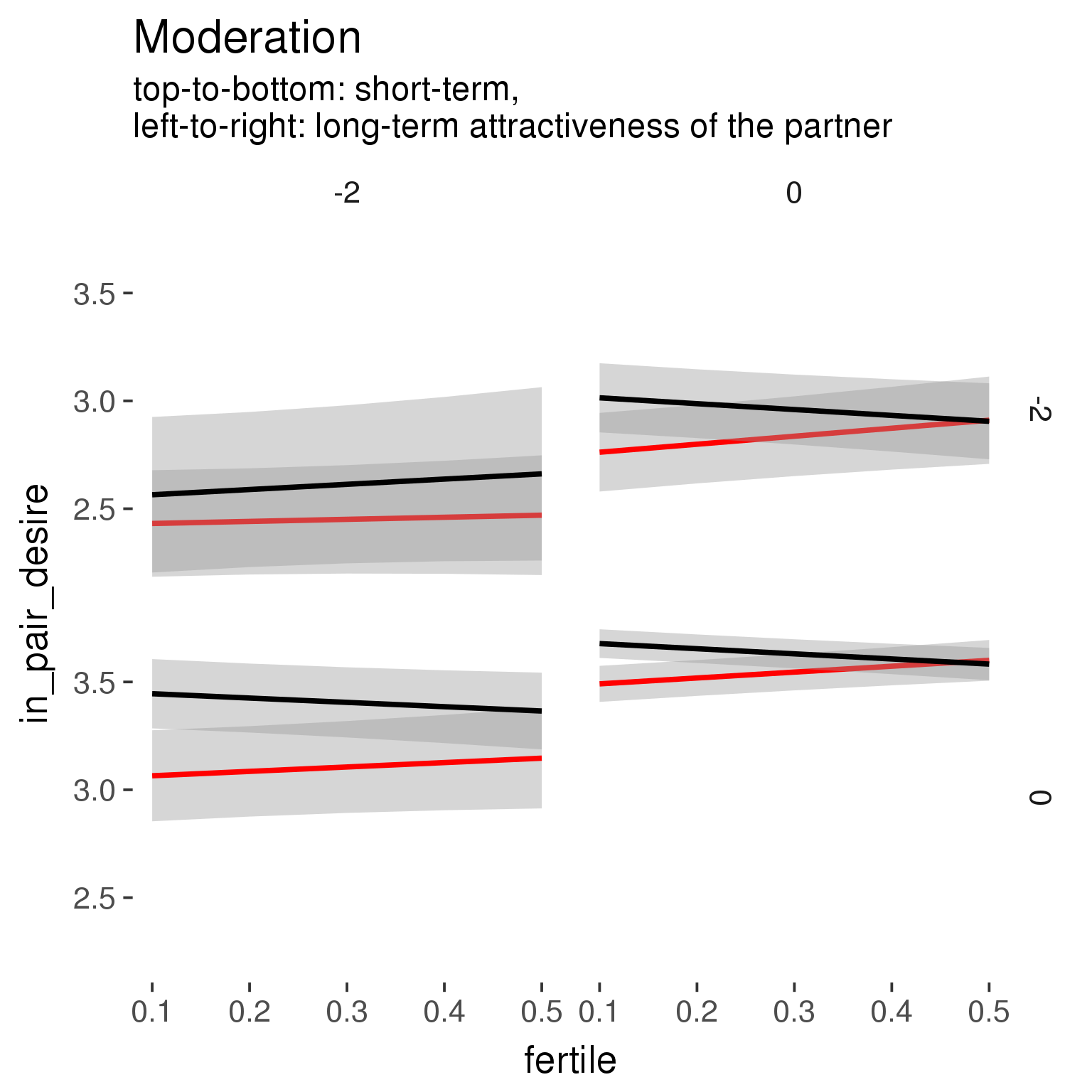
print_summary(with_mod)Linear mixed model fit by REML ['lmerMod']
Formula: in_pair_desire ~ menstruation + fertile_mean + (1 | person) +
partner_attractiveness_longterm + fertile + partner_attractiveness_shortterm +
included + menstruation:included + partner_attractiveness_longterm:fertile +
partner_attractiveness_longterm:partner_attractiveness_shortterm +
fertile:partner_attractiveness_shortterm + partner_attractiveness_longterm:included +
fertile:included + partner_attractiveness_shortterm:included +
partner_attractiveness_longterm:fertile:partner_attractiveness_shortterm +
partner_attractiveness_longterm:fertile:included + partner_attractiveness_longterm:partner_attractiveness_shortterm:included +
fertile:partner_attractiveness_shortterm:included + partner_attractiveness_longterm:fertile:partner_attractiveness_shortterm:included
Data: diary
REML criterion at convergence: 82884
Scaled residuals:
Min 1Q Median 3Q Max
-3.469 -0.679 -0.031 0.666 3.721
Random effects:
Groups Name Variance Std.Dev.
person (Intercept) 0.571 0.756
Residual 1.188 1.090
Number of obs: 26680, groups: person, 1054
Fixed effects:
Estimate
(Intercept) 3.50204
menstruationpre -0.06820
menstruationyes -0.18859
fertile_mean 0.03909
partner_attractiveness_longterm 0.20962
fertile 0.27279
partner_attractiveness_shortterm 0.36951
includedhorm_contra 0.23158
menstruationpre:includedhorm_contra -0.00223
menstruationyes:includedhorm_contra 0.03739
partner_attractiveness_longterm:fertile 0.03446
partner_attractiveness_longterm:partner_attractiveness_shortterm 0.02908
fertile:partner_attractiveness_shortterm -0.04912
partner_attractiveness_longterm:includedhorm_contra -0.09155
fertile:includedhorm_contra -0.51024
partner_attractiveness_shortterm:includedhorm_contra -0.03942
partner_attractiveness_longterm:fertile:partner_attractiveness_shortterm -0.05152
partner_attractiveness_longterm:fertile:includedhorm_contra -0.05296
partner_attractiveness_longterm:partner_attractiveness_shortterm:includedhorm_contra -0.09524
fertile:partner_attractiveness_shortterm:includedhorm_contra 0.06646
partner_attractiveness_longterm:fertile:partner_attractiveness_shortterm:includedhorm_contra 0.17079
Std. Error
(Intercept) 0.07067
menstruationpre 0.03324
menstruationyes 0.03134
fertile_mean 0.31724
partner_attractiveness_longterm 0.04751
fertile 0.07023
partner_attractiveness_shortterm 0.04371
includedhorm_contra 0.05905
menstruationpre:includedhorm_contra 0.04267
menstruationyes:includedhorm_contra 0.04107
partner_attractiveness_longterm:fertile 0.06782
partner_attractiveness_longterm:partner_attractiveness_shortterm 0.03494
fertile:partner_attractiveness_shortterm 0.06152
partner_attractiveness_longterm:includedhorm_contra 0.06055
fertile:includedhorm_contra 0.08848
partner_attractiveness_shortterm:includedhorm_contra 0.05692
partner_attractiveness_longterm:fertile:partner_attractiveness_shortterm 0.05026
partner_attractiveness_longterm:fertile:includedhorm_contra 0.08603
partner_attractiveness_longterm:partner_attractiveness_shortterm:includedhorm_contra 0.05454
fertile:partner_attractiveness_shortterm:includedhorm_contra 0.07888
partner_attractiveness_longterm:fertile:partner_attractiveness_shortterm:includedhorm_contra 0.07783
t value
(Intercept) 49.6
menstruationpre -2.1
menstruationyes -6.0
fertile_mean 0.1
partner_attractiveness_longterm 4.4
fertile 3.9
partner_attractiveness_shortterm 8.5
includedhorm_contra 3.9
menstruationpre:includedhorm_contra -0.1
menstruationyes:includedhorm_contra 0.9
partner_attractiveness_longterm:fertile 0.5
partner_attractiveness_longterm:partner_attractiveness_shortterm 0.8
fertile:partner_attractiveness_shortterm -0.8
partner_attractiveness_longterm:includedhorm_contra -1.5
fertile:includedhorm_contra -5.8
partner_attractiveness_shortterm:includedhorm_contra -0.7
partner_attractiveness_longterm:fertile:partner_attractiveness_shortterm -1.0
partner_attractiveness_longterm:fertile:includedhorm_contra -0.6
partner_attractiveness_longterm:partner_attractiveness_shortterm:includedhorm_contra -1.7
fertile:partner_attractiveness_shortterm:includedhorm_contra 0.8
partner_attractiveness_longterm:fertile:partner_attractiveness_shortterm:includedhorm_contra 2.2
Relative attractiveness to self
whole MV and MV_P scale
Predicted fertile phase effect sizes (in red): biggest (EP desire, partner mate retention)/smallest (IP desire) when partner’s relative attractiveness is low.
three item subsets of the MV/MV_P scale
model %>%
test_moderator("partner_attractiveness_rel_to_self_MV_short", diary)refitting model(s) with ML (instead of REML)
| Df | AIC | BIC | logLik | deviance | Chisq | Chi Df | Pr(>Chisq) | |
|---|---|---|---|---|---|---|---|---|
| with_main | 13 | 83073 | 83179 | -41523 | 83047 | NA | NA | NA |
| with_mod | 15 | 83074 | 83196 | -41522 | 83044 | 2.942 | 2 | 0.2297 |
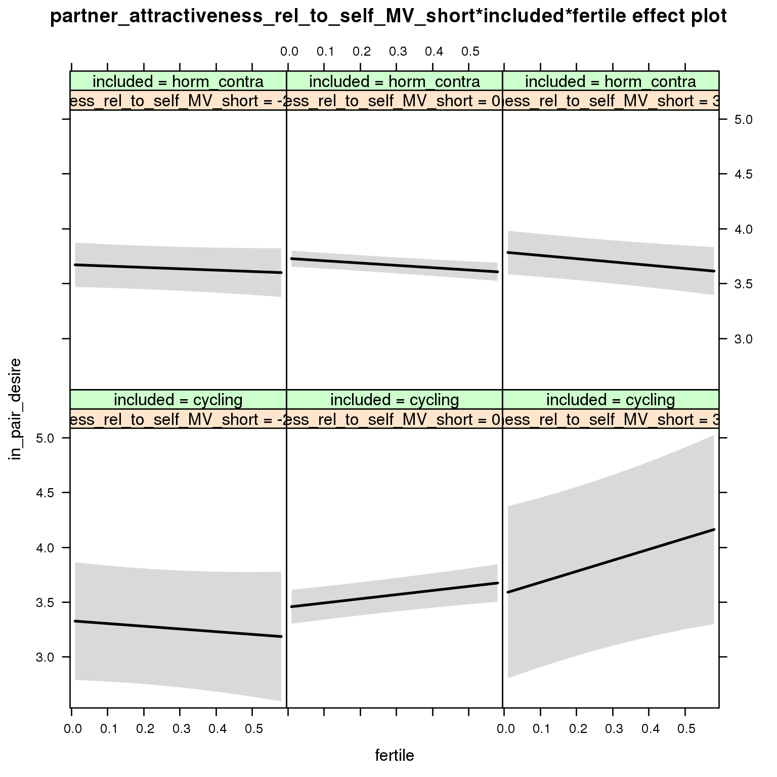
Linear mixed model fit by REML ['lmerMod']
Formula: in_pair_desire ~ menstruation + fertile_mean + (1 | person) +
partner_attractiveness_rel_to_self_MV_short + included +
fertile + menstruation:included + partner_attractiveness_rel_to_self_MV_short:included +
partner_attractiveness_rel_to_self_MV_short:fertile + included:fertile +
partner_attractiveness_rel_to_self_MV_short:included:fertile
Data: diary
REML criterion at convergence: 83097
Scaled residuals:
Min 1Q Median 3Q Max
-3.478 -0.678 -0.031 0.666 3.792
Random effects:
Groups Name Variance Std.Dev.
person (Intercept) 0.737 0.859
Residual 1.189 1.090
Number of obs: 26680, groups: person, 1054
Fixed effects:
Estimate Std. Error t value
(Intercept) 3.48531 0.08488 41.1
menstruationpre -0.06752 0.03327 -2.0
menstruationyes -0.18644 0.03135 -5.9
fertile_mean 0.02679 0.34747 0.1
partner_attractiveness_rel_to_self_MV_short 0.03999 0.10675 0.4
includedhorm_contra 0.27436 0.07253 3.8
fertile 0.32763 0.07982 4.1
menstruationpre:includedhorm_contra -0.00276 0.04271 -0.1
menstruationyes:includedhorm_contra 0.03701 0.04110 0.9
partner_attractiveness_rel_to_self_MV_short:includedhorm_contra -0.02178 0.11100 -0.2
partner_attractiveness_rel_to_self_MV_short:fertile 0.19950 0.12973 1.5
includedhorm_contra:fertile -0.53130 0.09605 -5.5
partner_attractiveness_rel_to_self_MV_short:includedhorm_contra:fertile -0.22710 0.13473 -1.7
model %>%
test_moderator("partner_attractiveness_rel_to_self", diary)refitting model(s) with ML (instead of REML)
| Df | AIC | BIC | logLik | deviance | Chisq | Chi Df | Pr(>Chisq) | |
|---|---|---|---|---|---|---|---|---|
| with_main | 13 | 83072 | 83178 | -41523 | 83046 | NA | NA | NA |
| with_mod | 15 | 83073 | 83196 | -41521 | 83043 | 2.917 | 2 | 0.2326 |
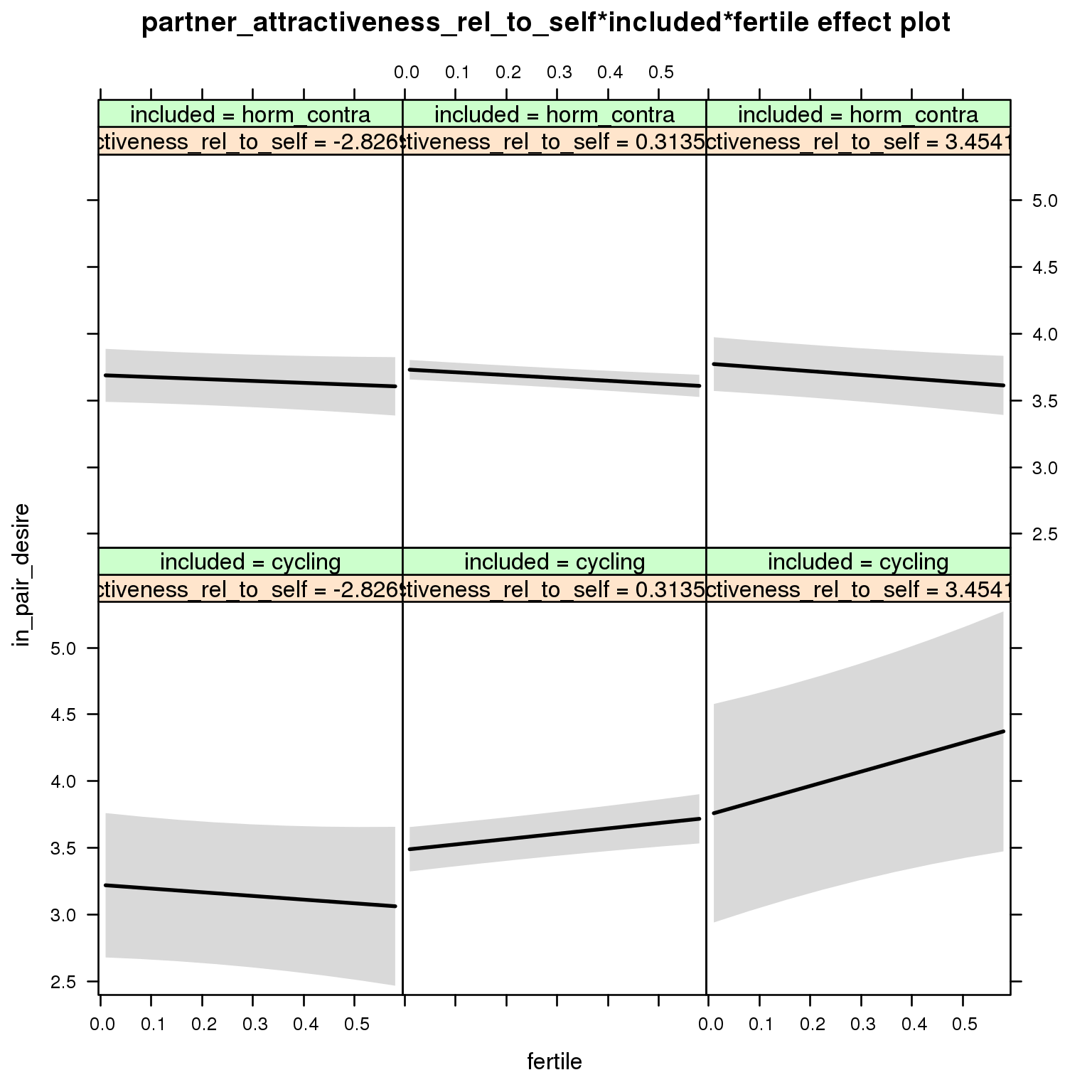
Linear mixed model fit by REML ['lmerMod']
Formula: in_pair_desire ~ menstruation + fertile_mean + (1 | person) +
partner_attractiveness_rel_to_self + included + fertile +
menstruation:included + partner_attractiveness_rel_to_self:included +
partner_attractiveness_rel_to_self:fertile + included:fertile +
partner_attractiveness_rel_to_self:included:fertile
Data: diary
REML criterion at convergence: 83097
Scaled residuals:
Min 1Q Median 3Q Max
-3.478 -0.679 -0.031 0.665 3.795
Random effects:
Groups Name Variance Std.Dev.
person (Intercept) 0.737 0.858
Residual 1.189 1.090
Number of obs: 26680, groups: person, 1054
Fixed effects:
Estimate Std. Error t value
(Intercept) 3.50059 0.08501 41.2
menstruationpre -0.06739 0.03327 -2.0
menstruationyes -0.18599 0.03136 -5.9
fertile_mean 0.02296 0.34736 0.1
partner_attractiveness_rel_to_self 0.08378 0.10964 0.8
includedhorm_contra 0.26103 0.07275 3.6
fertile 0.33222 0.08038 4.1
menstruationpre:includedhorm_contra -0.00294 0.04271 -0.1
menstruationyes:includedhorm_contra 0.03646 0.04111 0.9
partner_attractiveness_rel_to_self:includedhorm_contra -0.07014 0.11374 -0.6
partner_attractiveness_rel_to_self:fertile 0.21507 0.13433 1.6
includedhorm_contra:fertile -0.53765 0.09652 -5.6
partner_attractiveness_rel_to_self:includedhorm_contra:fertile -0.23666 0.13917 -1.7
Partner’s shortterm attractiveness, alternative specification
model %>%
test_moderator("partner_attractiveness_shortterm_v2", diary)refitting model(s) with ML (instead of REML)
| Df | AIC | BIC | logLik | deviance | Chisq | Chi Df | Pr(>Chisq) | |
|---|---|---|---|---|---|---|---|---|
| with_main | 13 | 82928 | 83035 | -41451 | 82902 | NA | NA | NA |
| with_mod | 15 | 82932 | 83055 | -41451 | 82902 | 0.1319 | 2 | 0.9362 |
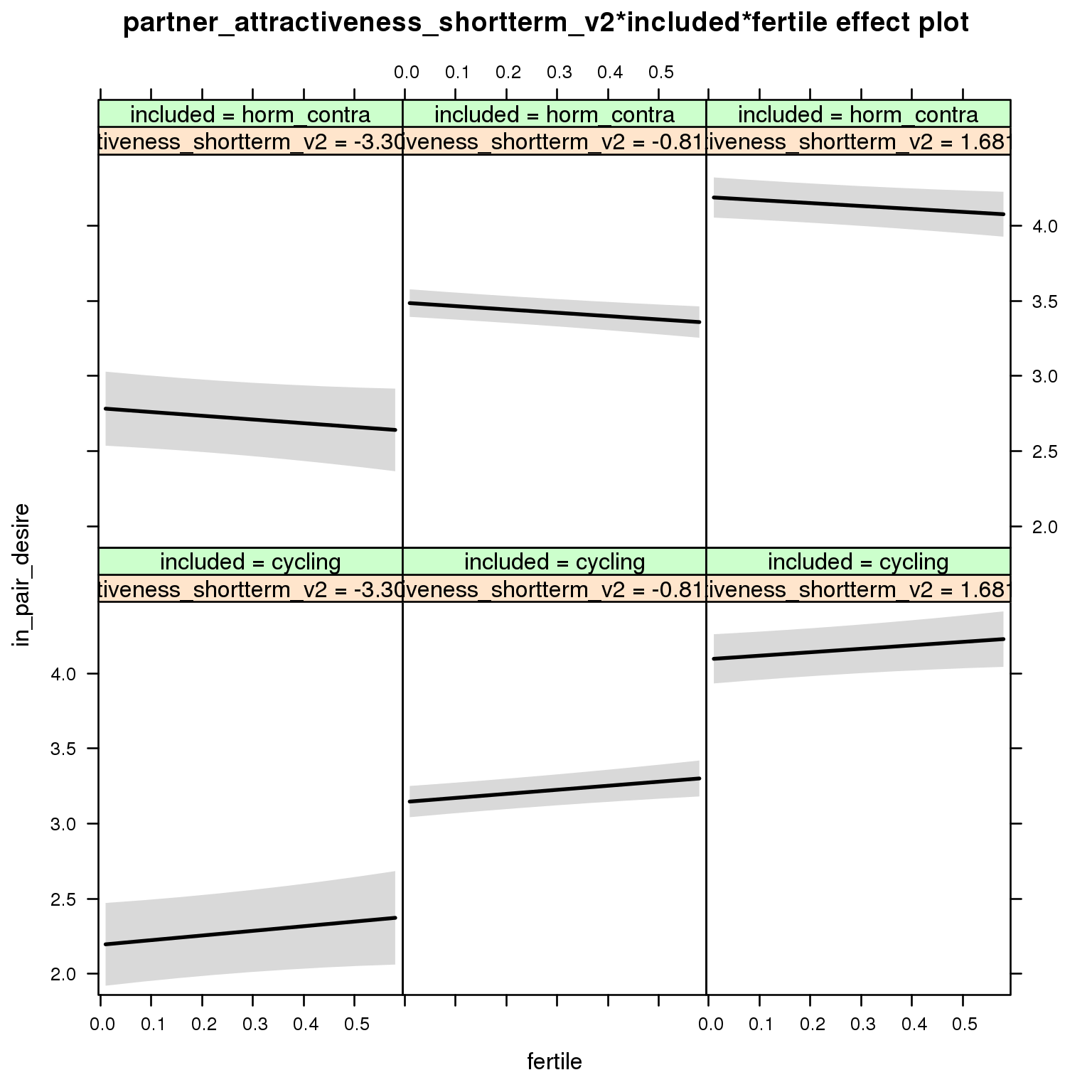
Linear mixed model fit by REML ['lmerMod']
Formula: in_pair_desire ~ menstruation + fertile_mean + (1 | person) +
partner_attractiveness_shortterm_v2 + included + fertile +
menstruation:included + partner_attractiveness_shortterm_v2:included +
partner_attractiveness_shortterm_v2:fertile + included:fertile +
partner_attractiveness_shortterm_v2:included:fertile
Data: diary
REML criterion at convergence: 82959
Scaled residuals:
Min 1Q Median 3Q Max
-3.489 -0.678 -0.030 0.665 3.753
Random effects:
Groups Name Variance Std.Dev.
person (Intercept) 0.636 0.797
Residual 1.188 1.090
Number of obs: 26680, groups: person, 1054
Fixed effects:
Estimate Std. Error t value
(Intercept) 3.51036 0.07161 49.0
menstruationpre -0.06955 0.03325 -2.1
menstruationyes -0.19054 0.03133 -6.1
fertile_mean -0.05967 0.32914 -0.2
partner_attractiveness_shortterm_v2 0.38131 0.04134 9.2
includedhorm_contra 0.25594 0.05857 4.4
fertile 0.25675 0.06715 3.8
menstruationpre:includedhorm_contra -0.00143 0.04269 0.0
menstruationyes:includedhorm_contra 0.03908 0.04107 1.0
partner_attractiveness_shortterm_v2:includedhorm_contra -0.09950 0.05485 -1.8
partner_attractiveness_shortterm_v2:fertile -0.01590 0.05613 -0.3
includedhorm_contra:fertile -0.46983 0.08510 -5.5
partner_attractiveness_shortterm_v2:includedhorm_contra:fertile 0.02649 0.07303 0.4
Partner’s global attractiveness
model %>%
test_moderator("partner_attractiveness_global", diary)refitting model(s) with ML (instead of REML)
| Df | AIC | BIC | logLik | deviance | Chisq | Chi Df | Pr(>Chisq) | |
|---|---|---|---|---|---|---|---|---|
| with_main | 13 | 83045 | 83152 | -41510 | 83019 | NA | NA | NA |
| with_mod | 15 | 83046 | 83169 | -41508 | 83016 | 3.289 | 2 | 0.1931 |
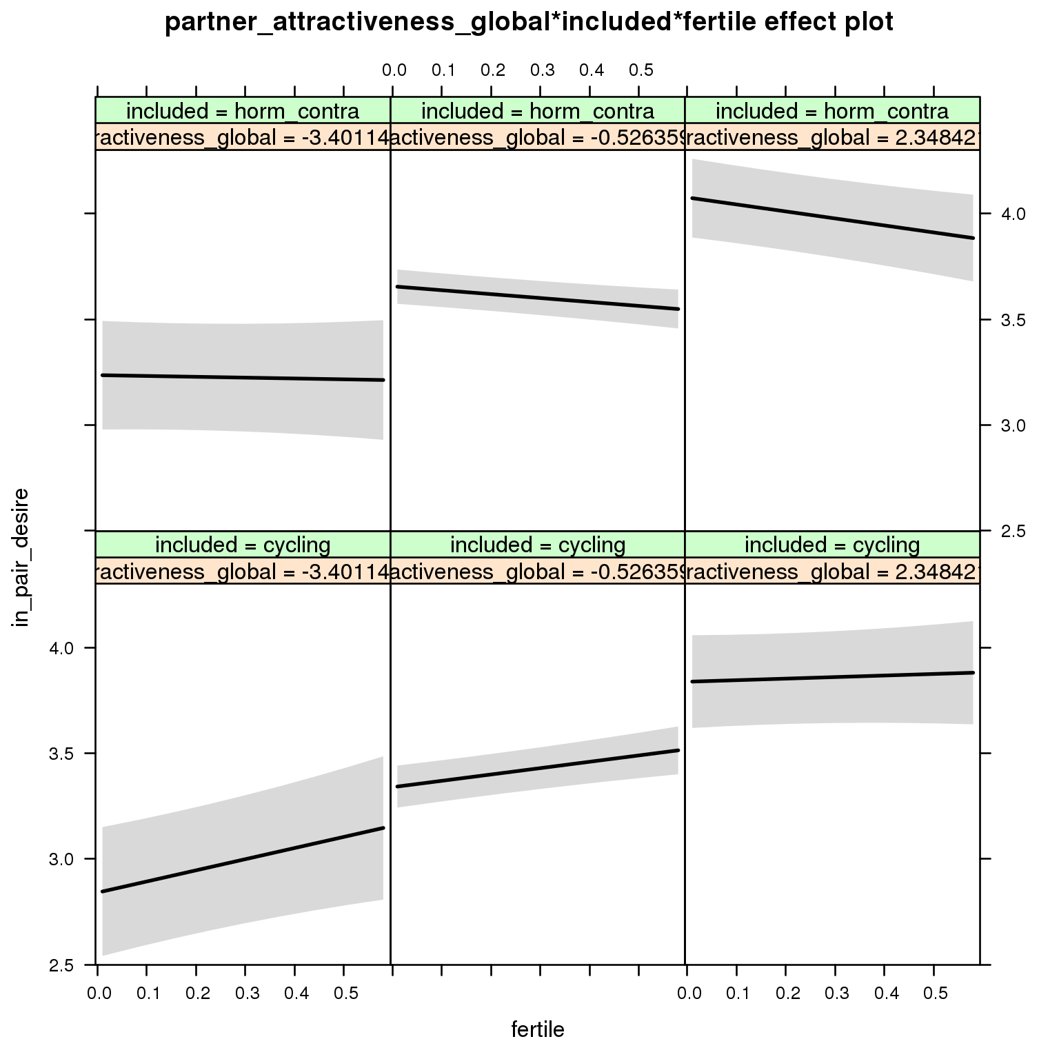
Linear mixed model fit by REML ['lmerMod']
Formula: in_pair_desire ~ menstruation + fertile_mean + (1 | person) +
partner_attractiveness_global + included + fertile + menstruation:included +
partner_attractiveness_global:included + partner_attractiveness_global:fertile +
included:fertile + partner_attractiveness_global:included:fertile
Data: diary
REML criterion at convergence: 83072
Scaled residuals:
Min 1Q Median 3Q Max
-3.465 -0.677 -0.031 0.664 3.781
Random effects:
Groups Name Variance Std.Dev.
person (Intercept) 0.717 0.846
Residual 1.189 1.090
Number of obs: 26680, groups: person, 1054
Fixed effects:
Estimate Std. Error t value
(Intercept) 3.48085 0.07485 46.5
menstruationpre -0.06830 0.03327 -2.1
menstruationyes -0.18857 0.03134 -6.0
fertile_mean -0.02659 0.34395 -0.1
partner_attractiveness_global 0.17364 0.04384 4.0
includedhorm_contra 0.29531 0.06124 4.8
fertile 0.25918 0.06714 3.9
menstruationpre:includedhorm_contra -0.00156 0.04271 0.0
menstruationyes:includedhorm_contra 0.03865 0.04109 0.9
partner_attractiveness_global:includedhorm_contra -0.02735 0.05749 -0.5
partner_attractiveness_global:fertile -0.07899 0.05567 -1.4
includedhorm_contra:fertile -0.47148 0.08504 -5.5
partner_attractiveness_global:includedhorm_contra:fertile 0.02826 0.07153 0.4
Partner’s longterm attractiveness
model %>%
test_moderator("partner_attractiveness_longterm", diary)refitting model(s) with ML (instead of REML)
| Df | AIC | BIC | logLik | deviance | Chisq | Chi Df | Pr(>Chisq) | |
|---|---|---|---|---|---|---|---|---|
| with_main | 13 | 82976 | 83082 | -41475 | 82950 | NA | NA | NA |
| with_mod | 15 | 82979 | 83102 | -41475 | 82949 | 0.5225 | 2 | 0.7701 |
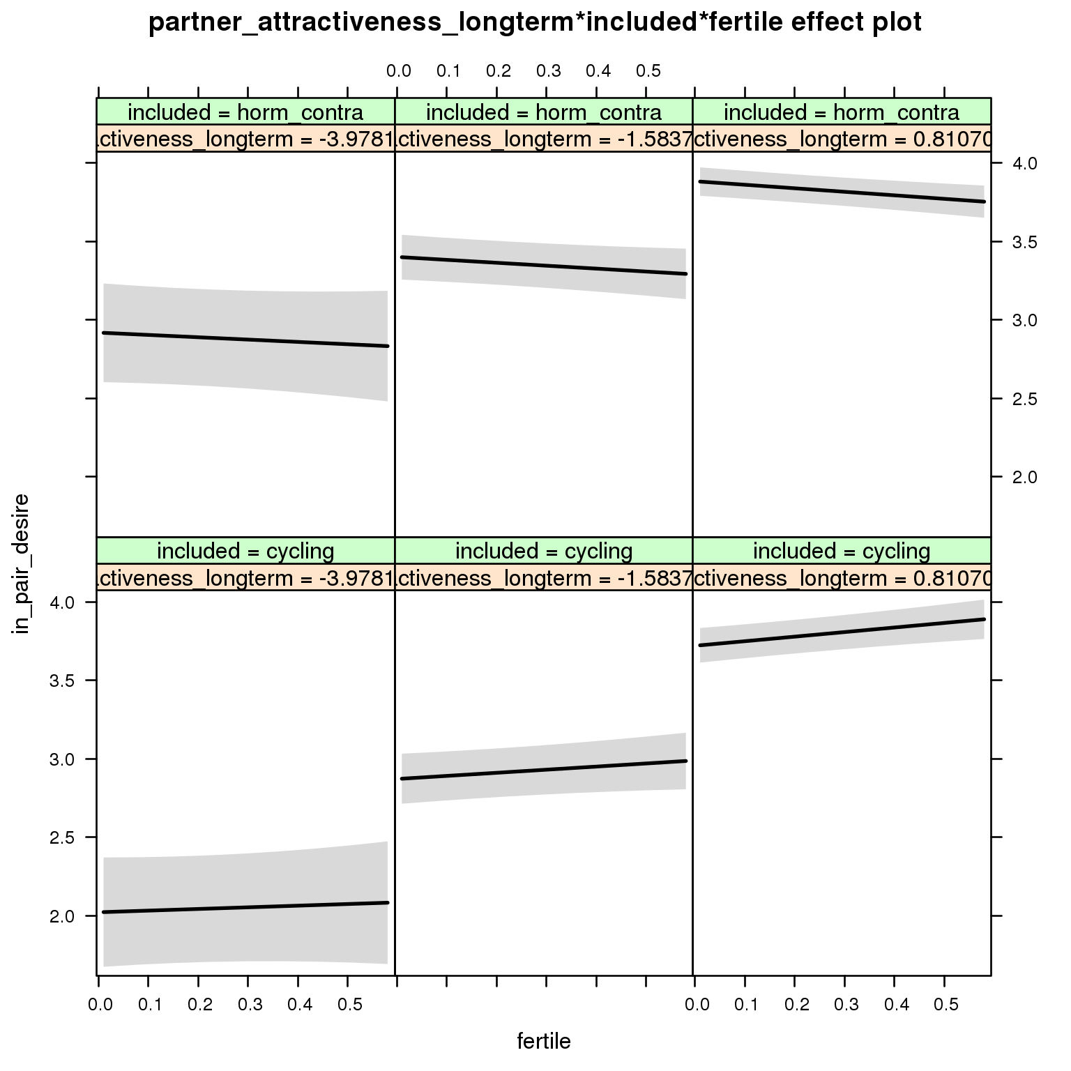
Linear mixed model fit by REML ['lmerMod']
Formula: in_pair_desire ~ menstruation + fertile_mean + (1 | person) +
partner_attractiveness_longterm + included + fertile + menstruation:included +
partner_attractiveness_longterm:included + partner_attractiveness_longterm:fertile +
included:fertile + partner_attractiveness_longterm:included:fertile
Data: diary
REML criterion at convergence: 83006
Scaled residuals:
Min 1Q Median 3Q Max
-3.475 -0.679 -0.030 0.666 3.784
Random effects:
Groups Name Variance Std.Dev.
person (Intercept) 0.669 0.818
Residual 1.188 1.090
Number of obs: 26680, groups: person, 1054
Fixed effects:
Estimate Std. Error t value
(Intercept) 3.45258 0.07293 47.3
menstruationpre -0.06861 0.03326 -2.1
menstruationyes -0.18796 0.03136 -6.0
fertile_mean 0.15132 0.33550 0.5
partner_attractiveness_longterm 0.35500 0.04347 8.2
includedhorm_contra 0.28065 0.05968 4.7
fertile 0.25971 0.06714 3.9
menstruationpre:includedhorm_contra -0.00185 0.04270 0.0
menstruationyes:includedhorm_contra 0.03799 0.04110 0.9
partner_attractiveness_longterm:includedhorm_contra -0.15338 0.05835 -2.6
partner_attractiveness_longterm:fertile 0.03883 0.05945 0.7
includedhorm_contra:fertile -0.47144 0.08512 -5.5
partner_attractiveness_longterm:includedhorm_contra:fertile -0.05470 0.07865 -0.7
Partner’s short-term vs. long-term attractiveness
We also test this specification of the short-term vs. long-term moderator prediction, but we think this is a suboptimal way to test it.
model %>%
test_moderator("partner_st_vs_lt", diary)refitting model(s) with ML (instead of REML)
| Df | AIC | BIC | logLik | deviance | Chisq | Chi Df | Pr(>Chisq) | |
|---|---|---|---|---|---|---|---|---|
| with_main | 13 | 83055 | 83161 | -41514 | 83029 | NA | NA | NA |
| with_mod | 15 | 83058 | 83180 | -41514 | 83028 | 1.37 | 2 | 0.504 |
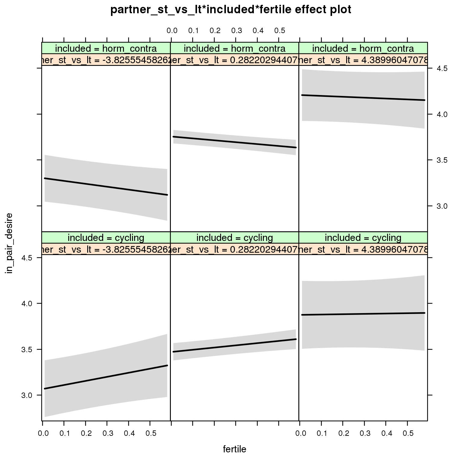
Linear mixed model fit by REML ['lmerMod']
Formula: in_pair_desire ~ menstruation + fertile_mean + (1 | person) +
partner_st_vs_lt + included + fertile + menstruation:included +
partner_st_vs_lt:included + partner_st_vs_lt:fertile + included:fertile +
partner_st_vs_lt:included:fertile
Data: diary
REML criterion at convergence: 83085
Scaled residuals:
Min 1Q Median 3Q Max
-3.494 -0.678 -0.031 0.667 3.787
Random effects:
Groups Name Variance Std.Dev.
person (Intercept) 0.722 0.85
Residual 1.189 1.09
Number of obs: 26680, groups: person, 1054
Fixed effects:
Estimate Std. Error t value
(Intercept) 3.49006 0.07541 46.3
menstruationpre -0.06726 0.03327 -2.0
menstruationyes -0.18709 0.03135 -6.0
fertile_mean -0.01312 0.34513 0.0
partner_st_vs_lt 0.09844 0.04082 2.4
includedhorm_contra 0.27531 0.06163 4.5
fertile 0.25414 0.06751 3.8
menstruationpre:includedhorm_contra -0.00364 0.04271 -0.1
menstruationyes:includedhorm_contra 0.03649 0.04110 0.9
partner_st_vs_lt:includedhorm_contra 0.01163 0.05195 0.2
partner_st_vs_lt:fertile -0.04967 0.05199 -1.0
includedhorm_contra:fertile -0.46828 0.08538 -5.5
partner_st_vs_lt:includedhorm_contra:fertile 0.07658 0.06554 1.2
Partner’s mate value
long scale
model %>%
test_moderator("MV_P", diary)refitting model(s) with ML (instead of REML)
| Df | AIC | BIC | logLik | deviance | Chisq | Chi Df | Pr(>Chisq) | |
|---|---|---|---|---|---|---|---|---|
| with_main | 13 | 83058 | 83164 | -41516 | 83032 | NA | NA | NA |
| with_mod | 15 | 83057 | 83180 | -41513 | 83027 | 4.971 | 2 | 0.08329 |
Error: Error in plot.eff(x[[(i - 1) * cols + j]], row = i, col = j, nrow = rows, : x.var = ‘fertile’ is not in the effect.
short scale
model %>%
test_moderator("MV_P_short", diary)refitting model(s) with ML (instead of REML)
| Df | AIC | BIC | logLik | deviance | Chisq | Chi Df | Pr(>Chisq) | |
|---|---|---|---|---|---|---|---|---|
| with_main | 13 | 83015 | 83121 | -41494 | 82989 | NA | NA | NA |
| with_mod | 15 | 83012 | 83134 | -41491 | 82982 | 7.202 | 2 | 0.0273 |
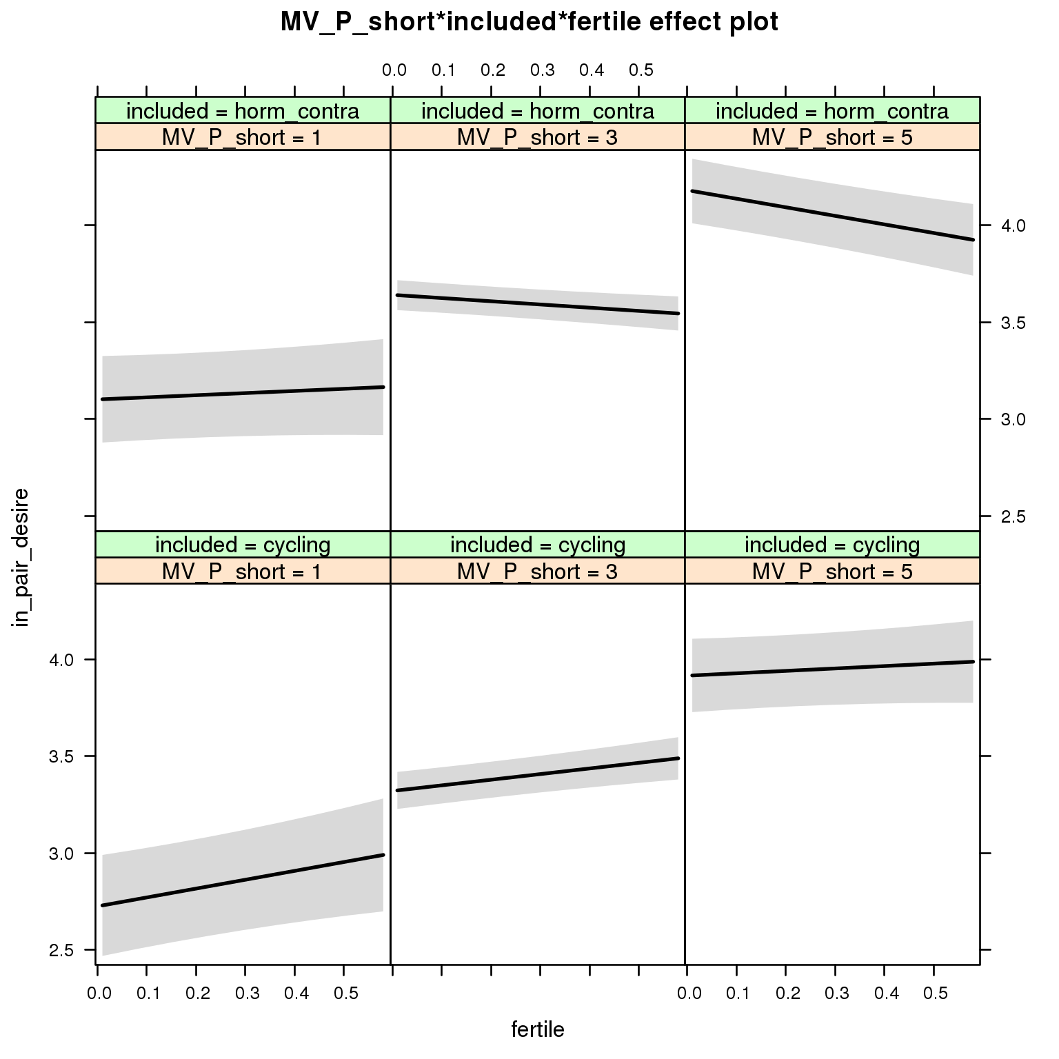
Linear mixed model fit by REML ['lmerMod']
Formula: in_pair_desire ~ menstruation + fertile_mean + (1 | person) +
MV_P_short + included + fertile + menstruation:included +
MV_P_short:included + MV_P_short:fertile + included:fertile + MV_P_short:included:fertile
Data: diary
REML criterion at convergence: 83036
Scaled residuals:
Min 1Q Median 3Q Max
-3.479 -0.680 -0.028 0.664 3.772
Random effects:
Groups Name Variance Std.Dev.
person (Intercept) 0.692 0.832
Residual 1.188 1.090
Number of obs: 26680, groups: person, 1054
Fixed effects:
Estimate Std. Error t value
(Intercept) 2.47636 0.19252 12.86
menstruationpre -0.06876 0.03326 -2.07
menstruationyes -0.18853 0.03134 -6.02
fertile_mean -0.02163 0.33951 -0.06
MV_P_short 0.29751 0.05289 5.63
includedhorm_contra 0.39626 0.24359 1.63
fertile 0.54022 0.24290 2.22
menstruationpre:includedhorm_contra -0.00105 0.04270 -0.02
menstruationyes:includedhorm_contra 0.03840 0.04108 0.93
MV_P_short:includedhorm_contra -0.02755 0.07028 -0.39
MV_P_short:fertile -0.08323 0.06947 -1.20
includedhorm_contra:fertile -0.29227 0.31384 -0.93
MV_P_short:includedhorm_contra:fertile -0.05470 0.09014 -0.61
Partner’s job and income
model %>%
test_moderator("partner_attractiveness_money", diary)refitting model(s) with ML (instead of REML)
| Df | AIC | BIC | logLik | deviance | Chisq | Chi Df | Pr(>Chisq) | |
|---|---|---|---|---|---|---|---|---|
| with_main | 13 | 83073 | 83179 | -41523 | 83047 | NA | NA | NA |
| with_mod | 15 | 83076 | 83199 | -41523 | 83046 | 0.6831 | 2 | 0.7107 |
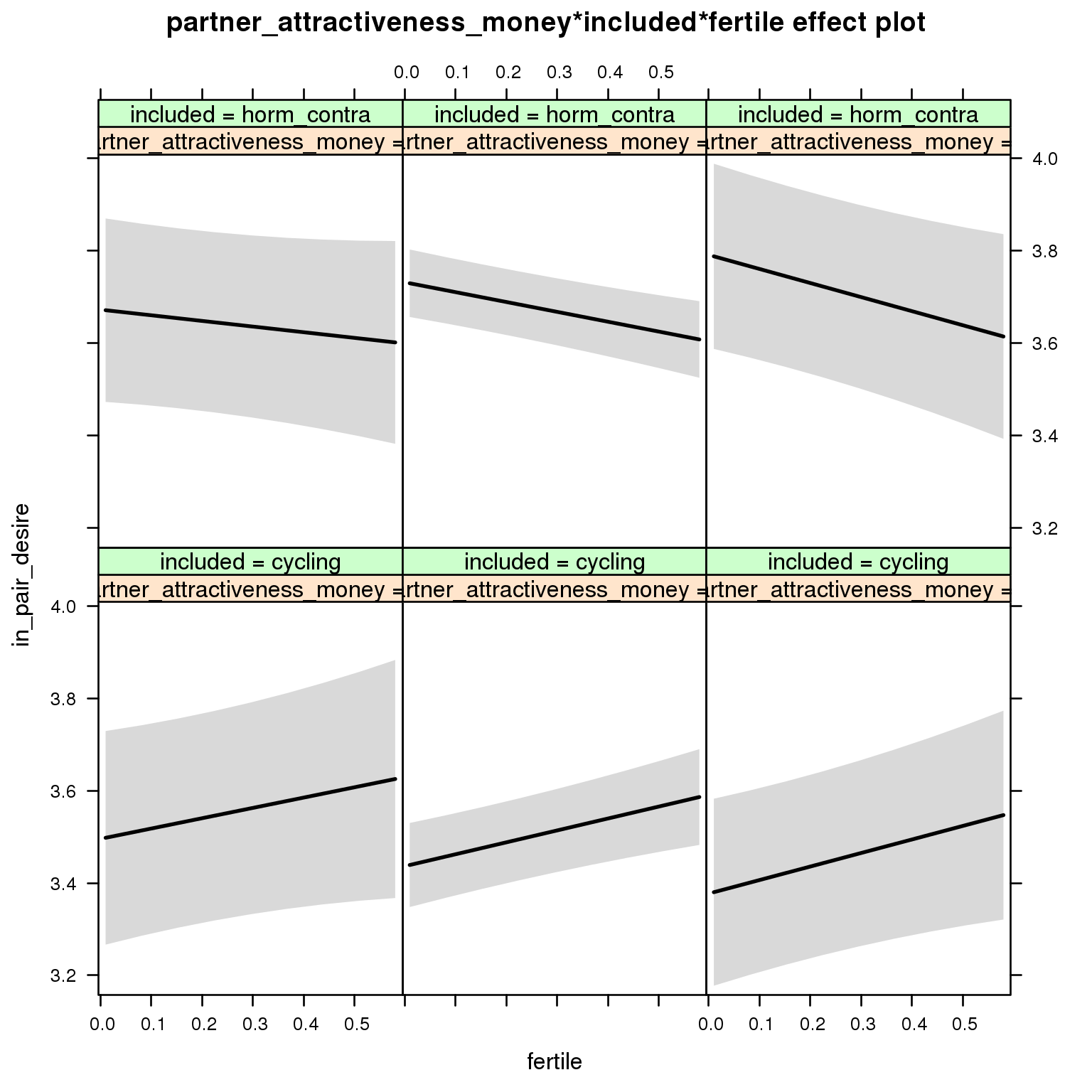
Linear mixed model fit by REML ['lmerMod']
Formula: in_pair_desire ~ menstruation + fertile_mean + (1 | person) +
partner_attractiveness_money + included + fertile + menstruation:included +
partner_attractiveness_money:included + partner_attractiveness_money:fertile +
included:fertile + partner_attractiveness_money:included:fertile
Data: diary
REML criterion at convergence: 83101
Scaled residuals:
Min 1Q Median 3Q Max
-3.492 -0.678 -0.031 0.666 3.794
Random effects:
Groups Name Variance Std.Dev.
person (Intercept) 0.737 0.858
Residual 1.189 1.090
Number of obs: 26680, groups: person, 1054
Fixed effects:
Estimate Std. Error t value
(Intercept) 3.56519 0.17753 20.08
menstruationpre -0.06767 0.03327 -2.03
menstruationyes -0.18773 0.03135 -5.99
fertile_mean 0.02803 0.34755 0.08
partner_attractiveness_money -0.02962 0.05048 -0.59
includedhorm_contra 0.11133 0.22241 0.50
fertile 0.20609 0.21358 0.96
menstruationpre:includedhorm_contra -0.00282 0.04271 -0.07
menstruationyes:includedhorm_contra 0.03763 0.04110 0.92
partner_attractiveness_money:includedhorm_contra 0.05924 0.06933 0.85
partner_attractiveness_money:fertile 0.01737 0.06392 0.27
includedhorm_contra:fertile -0.28289 0.28031 -1.01
partner_attractiveness_money:includedhorm_contra:fertile -0.06293 0.08661 -0.73
Self-reported perceived desirability
model_summaries$desirability_1Model summary
Model summary
model %>%
print_summary()Linear mixed model fit by REML
t-tests use Satterthwaite approximations to degrees of freedom ['lmerMod']
Formula: desirability_1 ~ included * (menstruation + fertile) + fertile_mean + (1 | person)
Data: diary
REML criterion at convergence: 84665
Scaled residuals:
Min 1Q Median 3Q Max
-4.054 -0.629 0.030 0.659 3.660
Random effects:
Groups Name Variance Std.Dev.
person (Intercept) 0.727 0.853
Residual 1.264 1.124
Number of obs: 26685, groups: person, 1054
Fixed effects:
Estimate Std. Error df t value Pr(>|t|)
(Intercept) 3.71137 0.07578 1448.00000 48.98 <2e-16 ***
includedhorm_contra 0.00628 0.06201 1419.00000 0.10 0.9193
menstruationpre -0.11113 0.03429 26038.00000 -3.24 0.0012 **
menstruationyes -0.25228 0.03231 26151.00000 -7.81 6e-15 ***
fertile 0.14751 0.06921 26018.00000 2.13 0.0331 *
fertile_mean 0.01695 0.34834 1569.00000 0.05 0.9612
includedhorm_contra:menstruationpre 0.02787 0.04402 26035.00000 0.63 0.5266
includedhorm_contra:menstruationyes 0.07101 0.04235 26127.00000 1.68 0.0936 .
includedhorm_contra:fertile -0.28646 0.08765 26150.00000 -3.27 0.0011 **
---
Signif. codes: 0 '***' 0.001 '**' 0.01 '*' 0.05 '.' 0.1 ' ' 1
Correlation of Fixed Effects:
(Intr) incld_ mnstrtnp mnstrtny fertil frtl_m inclddhrm_cntr:mnstrtnp
inclddhrm_c -0.473
menstrutnpr -0.175 0.221
menstrutnys -0.170 0.213 0.397
fertile -0.167 0.273 0.467 0.384
fertile_men -0.772 -0.026 -0.008 -0.005 -0.071
inclddhrm_cntr:mnstrtnp 0.144 -0.277 -0.779 -0.309 -0.363 -0.004
inclddhrm_cntr:mnstrtny 0.136 -0.262 -0.303 -0.763 -0.292 -0.004 0.382
inclddhrm_cntr:f 0.167 -0.345 -0.368 -0.303 -0.786 0.010 0.466
inclddhrm_cntr:mnstrtny
inclddhrm_c
menstrutnpr
menstrutnys
fertile
fertile_men
inclddhrm_cntr:mnstrtnp
inclddhrm_cntr:mnstrtny
inclddhrm_cntr:f 0.381
Effect size standardised by residual variance (\(\frac{b}{ SD_{residual} }\)): 0.13 [0.01;0.25].
Marginal effect plots
model %>%
plot_all_effects()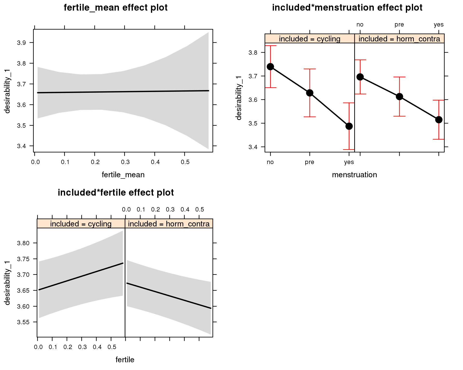
Outcome distribution
model %>%
plot_outcome(diary) + xlab(outcome_label)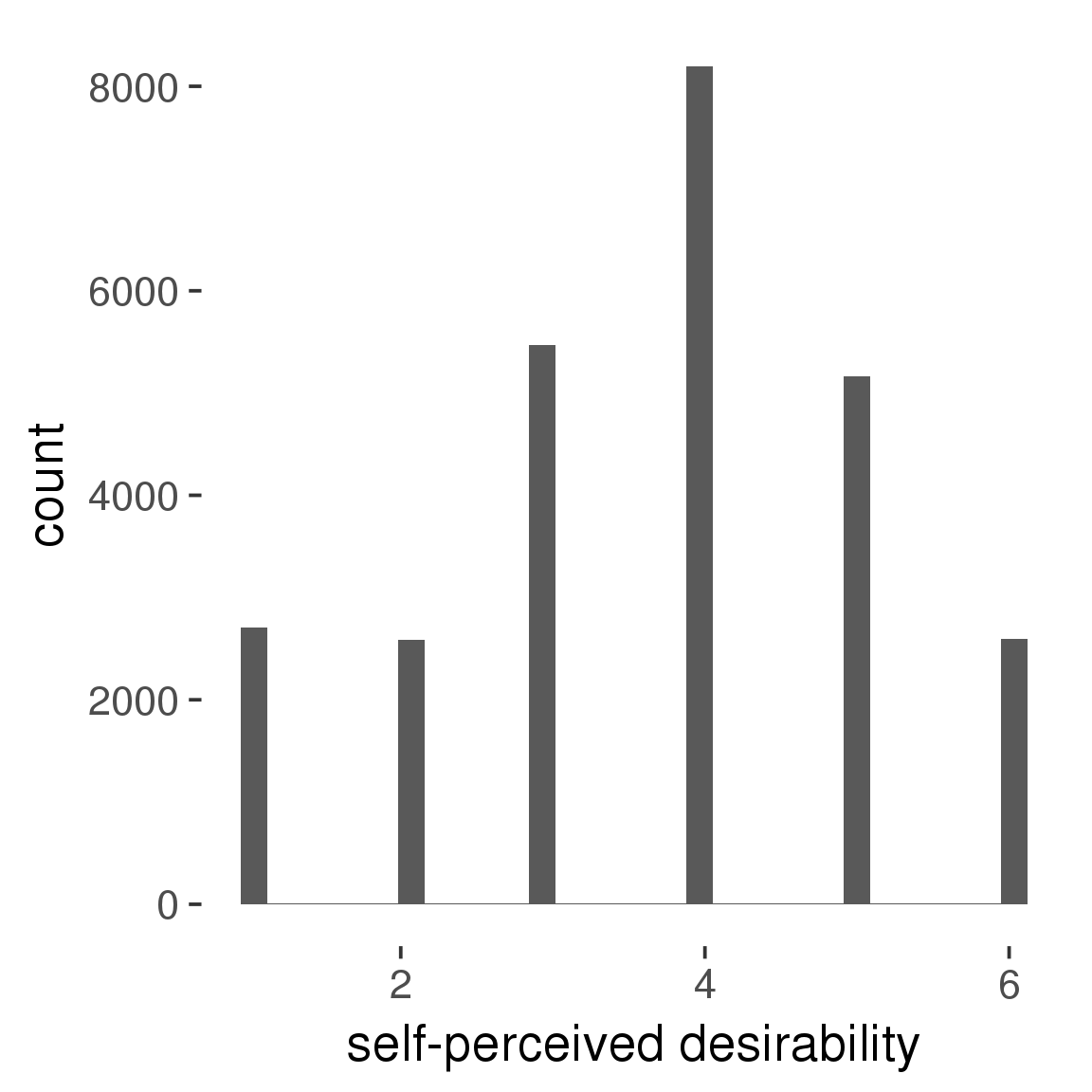
Diagnostics
model %>%
print_diagnostics()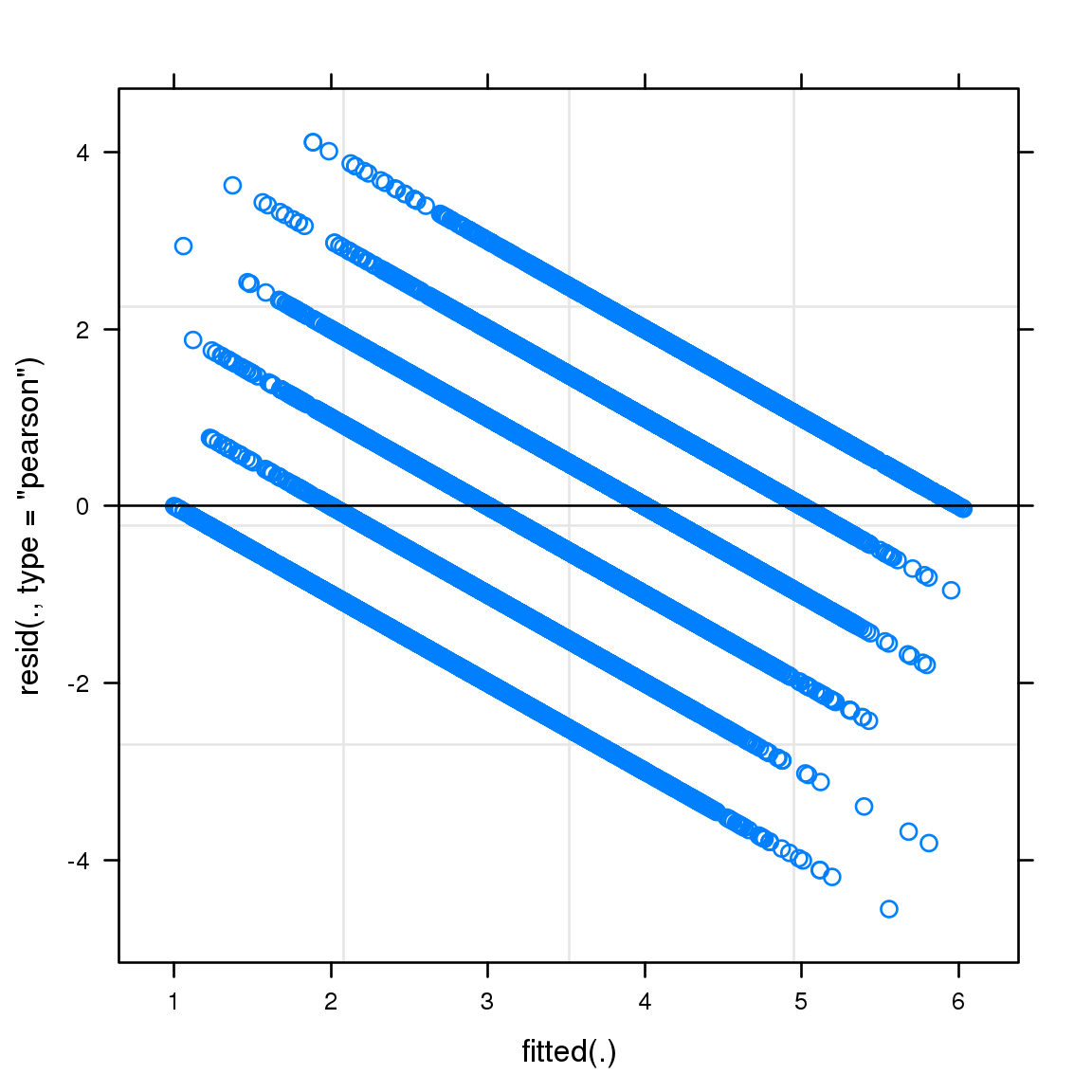
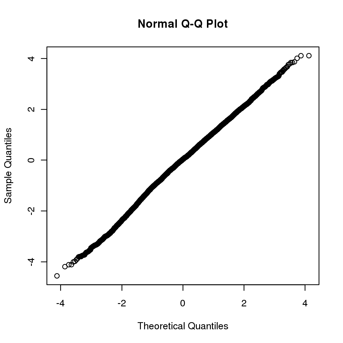

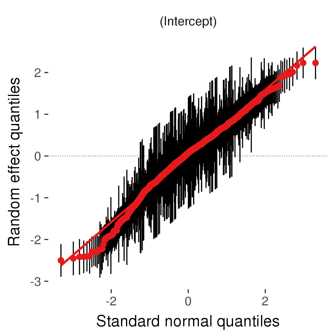
Curves
Here, we continuously plot the outcome over the course of the cycle. Because cycle lengths vary, we subset the data to cycles in a certain range. If the red curve traces the pink curve, our predictor accurately maps the relationship between fertile window probability and the outcome.
Cycle lengths from 21 to 36
Backward-counted
model %>%
plot_curve(diary %>% filter(minimum_cycle_length_diary <= 36, minimum_cycle_length_diary > 20) %>% mutate(fertile=prc_stirn_b))outcome = names(model@frame)[1]
outcome_label = recode(str_replace_all(str_replace_all(str_replace_all(outcome, "_", " "), " pair", "-pair"), " 1", ""),
"desirability 1" = "self-perceived desirability",
"NARQ admiration" = "narcissistic admiration",
"NARQ rivalry" = "narcissistic rivalry",
"extra-pair" = "extra-pair desire & behaviour",
"had sexual intercourse" = "sexual intercourse")
library(ggplot2)
# form a subset and run the model without the hormonal contraception and the fertility predictors
tmp = diary %>%
filter(!is.na(fertile), !is.na(included),
RCD > -1 * minimum_cycle_length_diary, RCD > -40)
new_form = update.formula(formula(model), new = . ~ . - fertile * included)
tmp$residuals = residuals(update(model, new_form, data = tmp , na.action = na.exclude))
tmp = tmp %>%
filter(!is.na(RCD), !is.na(residuals))
rcd_min = min(tmp$RCD)
tmp$real = FALSE
tmp_before = tmp
tmp_before$RCD = tmp_before$RCD + min(tmp$RCD) - 1
tmp_after = tmp
tmp_after$RCD = tmp_after$RCD - min(tmp$RCD) + 1
tmp$real = TRUE
tmp = bind_rows(tmp_before %>% filter(RCD > rcd_min - 11), tmp, tmp_after %>% filter(RCD < 11))GAM smooth on residuals
Here, we partialled out menstruation and individual random effects, then superimposed estimated probability of being in the fertile window scaled to the range of the estimated means. To address the periodicity of the cycle, we prepended and appended ten days of the timeseries to the end and the beginning of the timeseries. We then estimated the GAM and cut off the appended subsets before plotting.
tryCatch({
trend_plot = ggplot(tmp,aes(x = RCD, y = residuals, colour = included)) +
stat_smooth(geom = 'smooth',size = 0.8, fill = "#9ECAE1", method = 'gam', formula = y ~ s(x))
}, error = function(e){cat_message(e, "danger")})
tryCatch({
trend_data = ggplot_build(trend_plot)$data[[1]]
}, error = function(e){cat_message(e, "danger")})
trend_data$RCD = round(trend_data$x)
trend_data = left_join(trend_data, tmp %>% select(real, RCD,fertile) %>% unique(), by = "RCD")
trend_data %>%
filter(real == TRUE) %>%
mutate(superimposed = ( ( (fertile - 0.01)/0.58) * (max(y)-min(y) ) ) + min(y) ) ->
trend_data
ggplot(trend_data) +
geom_ribbon(aes(x = x, ymin = ymin, ymax = ymax, fill = factor(group)), alpha = 0.2) +
geom_line(aes(x = x, y = y, colour = factor(group)), size = 0.8, stat = "identity") +
scale_x_continuous(caption_x) +
geom_line(aes(x = x, y = superimposed), color = "#a83fbf", size = 1, linetype = 'dashed') +
annotate("text",x = mean(trend_data$x), y = max(trend_data$superimposed,na.rm=T) + 0.1, label = 'superimposed fertility peak', color = "#a83fbf") +
scale_y_continuous(outcome_label) +
ggtitle("GAM smooth, residuals") +
scale_color_manual("Contraception status",values = c("2"="black","1"= "red"), labels = c("2"="hormonally\ncontracepting","1"="cycling"), guide = F) +
scale_fill_manual("Contraception status",values = c("2"="black","1"= "red"), labels = c("2"="hormonally\ncontracepting","1"="cycling"), guide = F)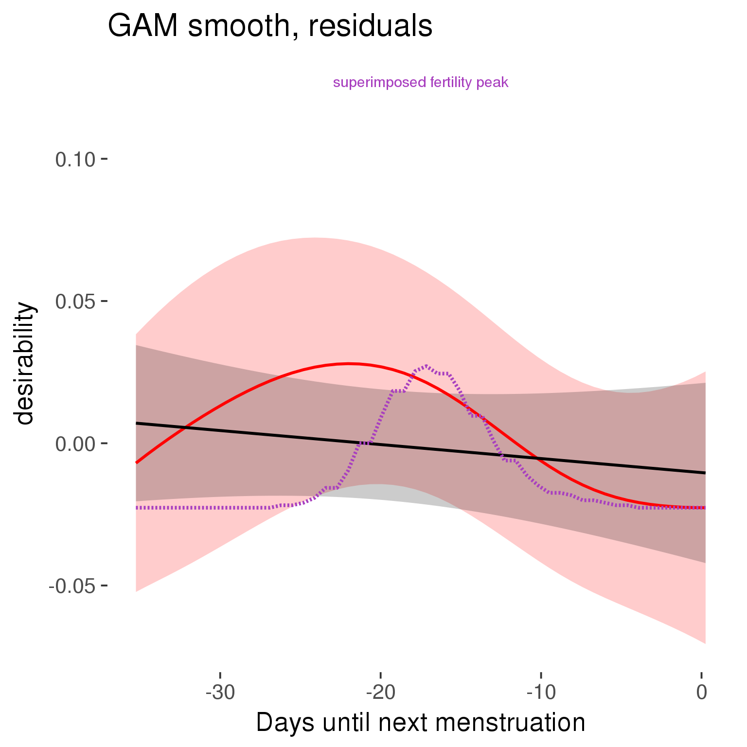
GAM smooth on raw data
As before, but without partialling anything out.
tryCatch({
trend_plot = ggplot(tmp,aes_string(x = "RCD", y = outcome, colour = "included")) +
stat_smooth(geom = 'smooth',size = 0.8, fill = "#9ECAE1", method = 'gam', formula = y ~ s(x))
}, error = function(e){cat_message(e, "danger")})
tryCatch({
trend_data = ggplot_build(trend_plot)$data[[1]]
}, error = function(e){cat_message(e, "danger")})
trend_data$RCD = round(trend_data$x)
trend_data = left_join(trend_data, tmp %>% select(real, RCD,fertile) %>% unique(), by = "RCD")
trend_data %>%
filter(real == TRUE) %>%
mutate(superimposed = ( ( (fertile - 0.01)/0.58) * (max(y)-min(y) ) ) + min(y) ) ->
trend_data
plot1b = ggplot(trend_data) +
geom_ribbon(aes(x = x, ymin = ymin, ymax = ymax, fill = factor(group)), alpha = 0.2) +
geom_line(aes(x = x, y = y, colour = factor(group)), size = 0.8, stat = "identity") +
scale_x_continuous(caption_x) +
geom_line(aes(x = x, y = superimposed), color = "#a83fbf", size = 1, linetype = 'dashed') +
annotate("text",x = mean(trend_data$x), y = max(trend_data$superimposed,na.rm=T) + 0.1, label = 'superimposed fertility peak', color = "#a83fbf") +
scale_y_continuous(outcome_label) +
ggtitle("GAM smooth, raw data") +
scale_color_manual("Contraception status",values = c("2"="black","1"= "red"), labels = c("2"="hormonally\ncontracepting","1"="cycling"), guide = F) +
scale_fill_manual("Contraception status",values = c("2"="black","1"= "red"), labels = c("2"="hormonally\ncontracepting","1"="cycling"), guide = F)
suppressWarnings(print(plot1b))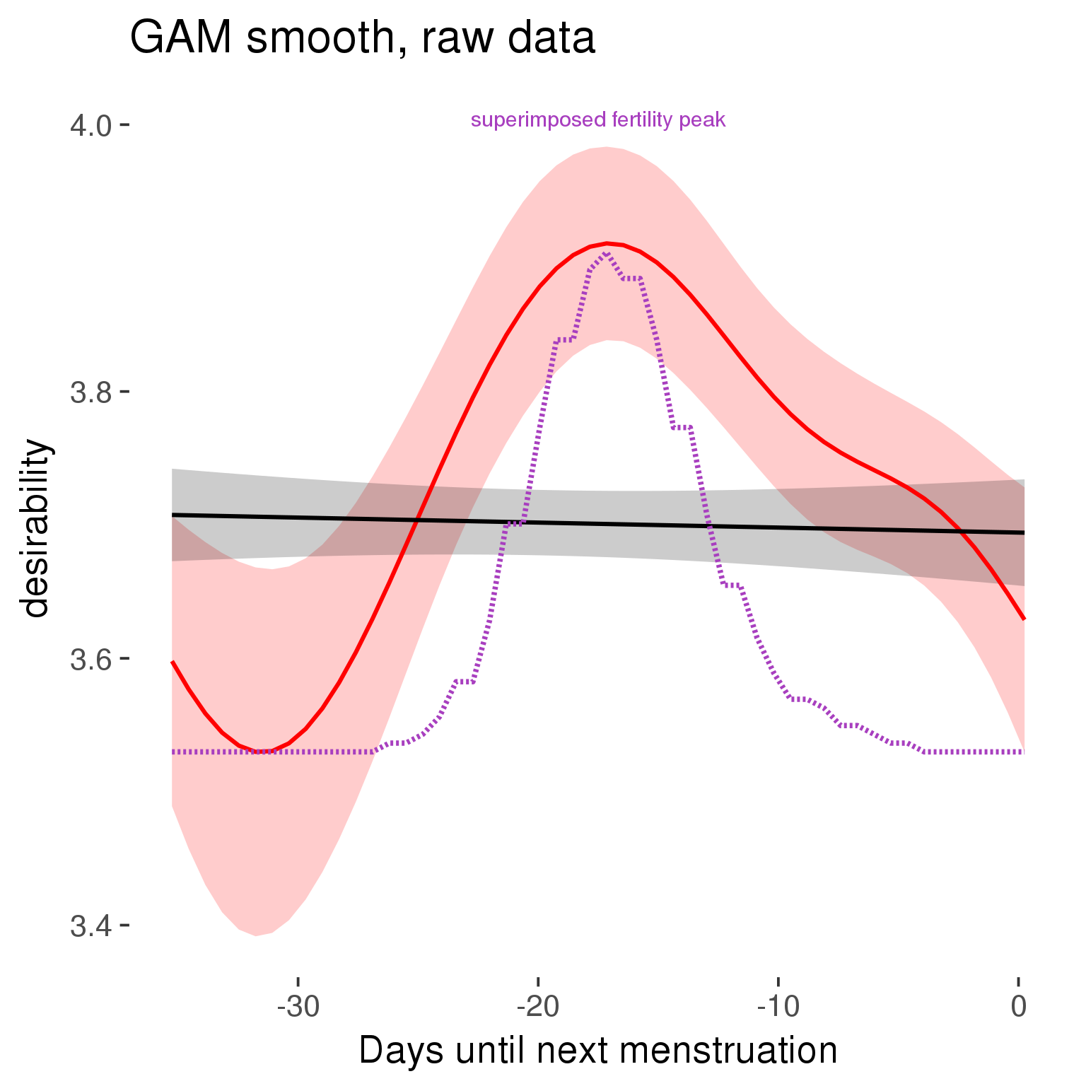
Means and standard errors over raw data
Nothing partialled out, just straight means with bootstrapped confidence intervals.
tryCatch({
trend_plot = ggplot(tmp,aes_string(x = "RCD", y = outcome, colour = "included")) +
geom_pointrange(size = 0.8, stat = 'summary', fun.data = "mean_cl_boot")
}, error = function(e){cat_message(e, "danger")})
tryCatch({
trend_data = ggplot_build(trend_plot)$data[[1]]
}, error = function(e){cat_message(e, "danger")})
trend_data$RCD = round(trend_data$x)
trend_data = left_join(trend_data, tmp %>% select(real, RCD,fertile) %>% unique(), by = "RCD")
trend_data %>%
filter(real == TRUE) %>%
mutate(superimposed = ( ( (fertile - 0.01)/0.58) * (max(y)-min(y) ) ) + min(y) ) ->
trend_data
plot3 = ggplot(trend_data) +
geom_pointrange(aes(x = x, y = y, ymin = ymin,ymax = ymax, colour = factor(group)), size = 0.8, stat = "identity", alpha = 0.6, position = position_dodge(width = .5)) +
scale_x_continuous("Days until next menstruation") +
geom_line(aes(x= x, y = superimposed), color = "#a83fbf", size = 1, linetype = 'dashed') +
annotate("text",x = mean(trend_data$x), y = max(trend_data$superimposed,na.rm=T) + 0.1, label = 'superimposed fertility peak', color = "#a83fbf") +
scale_y_continuous(outcome_label) +
ggtitle("Means with standard errors, raw data") +
scale_color_manual("Contraception status",values = c("2"="black","1"= "red"), labels = c("2"="hormonally\ncontracepting","1"="cycling"), guide = F) +
scale_fill_manual("Contraception status",values = c("2"="black","1"= "red"), labels = c("2"="hormonally\ncontracepting","1"="cycling"), guide = F)
suppressWarnings(print(plot3))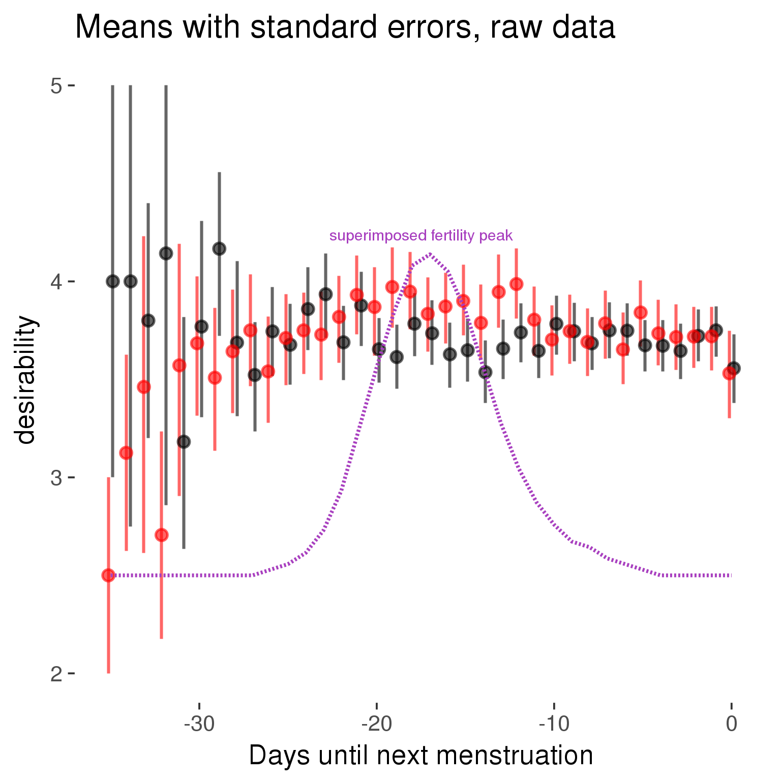
Forward-counted
model %>%
plot_curve(diary %>% filter(minimum_cycle_length_diary <= 36, minimum_cycle_length_diary > 20) %>% mutate(RCD = FCD, fertile = prc_stirn_b_forward_counted), caption_x = "Days since last menstruation")outcome = names(model@frame)[1]
outcome_label = recode(str_replace_all(str_replace_all(str_replace_all(outcome, "_", " "), " pair", "-pair"), " 1", ""),
"desirability 1" = "self-perceived desirability",
"NARQ admiration" = "narcissistic admiration",
"NARQ rivalry" = "narcissistic rivalry",
"extra-pair" = "extra-pair desire & behaviour",
"had sexual intercourse" = "sexual intercourse")
library(ggplot2)
# form a subset and run the model without the hormonal contraception and the fertility predictors
tmp = diary %>%
filter(!is.na(fertile), !is.na(included),
RCD > -1 * minimum_cycle_length_diary, RCD > -40)
new_form = update.formula(formula(model), new = . ~ . - fertile * included)
tmp$residuals = residuals(update(model, new_form, data = tmp , na.action = na.exclude))
tmp = tmp %>%
filter(!is.na(RCD), !is.na(residuals))
rcd_min = min(tmp$RCD)
tmp$real = FALSE
tmp_before = tmp
tmp_before$RCD = tmp_before$RCD + min(tmp$RCD) - 1
tmp_after = tmp
tmp_after$RCD = tmp_after$RCD - min(tmp$RCD) + 1
tmp$real = TRUE
tmp = bind_rows(tmp_before %>% filter(RCD > rcd_min - 11), tmp, tmp_after %>% filter(RCD < 11))GAM smooth on residuals
Here, we partialled out menstruation and individual random effects, then superimposed estimated probability of being in the fertile window scaled to the range of the estimated means. To address the periodicity of the cycle, we prepended and appended ten days of the timeseries to the end and the beginning of the timeseries. We then estimated the GAM and cut off the appended subsets before plotting.
tryCatch({
trend_plot = ggplot(tmp,aes(x = RCD, y = residuals, colour = included)) +
stat_smooth(geom = 'smooth',size = 0.8, fill = "#9ECAE1", method = 'gam', formula = y ~ s(x))
}, error = function(e){cat_message(e, "danger")})
tryCatch({
trend_data = ggplot_build(trend_plot)$data[[1]]
}, error = function(e){cat_message(e, "danger")})
trend_data$RCD = round(trend_data$x)
trend_data = left_join(trend_data, tmp %>% select(real, RCD,fertile) %>% unique(), by = "RCD")
trend_data %>%
filter(real == TRUE) %>%
mutate(superimposed = ( ( (fertile - 0.01)/0.58) * (max(y)-min(y) ) ) + min(y) ) ->
trend_data
ggplot(trend_data) +
geom_ribbon(aes(x = x, ymin = ymin, ymax = ymax, fill = factor(group)), alpha = 0.2) +
geom_line(aes(x = x, y = y, colour = factor(group)), size = 0.8, stat = "identity") +
scale_x_continuous(caption_x) +
geom_line(aes(x = x, y = superimposed), color = "#a83fbf", size = 1, linetype = 'dashed') +
annotate("text",x = mean(trend_data$x), y = max(trend_data$superimposed,na.rm=T) + 0.1, label = 'superimposed fertility peak', color = "#a83fbf") +
scale_y_continuous(outcome_label) +
ggtitle("GAM smooth, residuals") +
scale_color_manual("Contraception status",values = c("2"="black","1"= "red"), labels = c("2"="hormonally\ncontracepting","1"="cycling"), guide = F) +
scale_fill_manual("Contraception status",values = c("2"="black","1"= "red"), labels = c("2"="hormonally\ncontracepting","1"="cycling"), guide = F)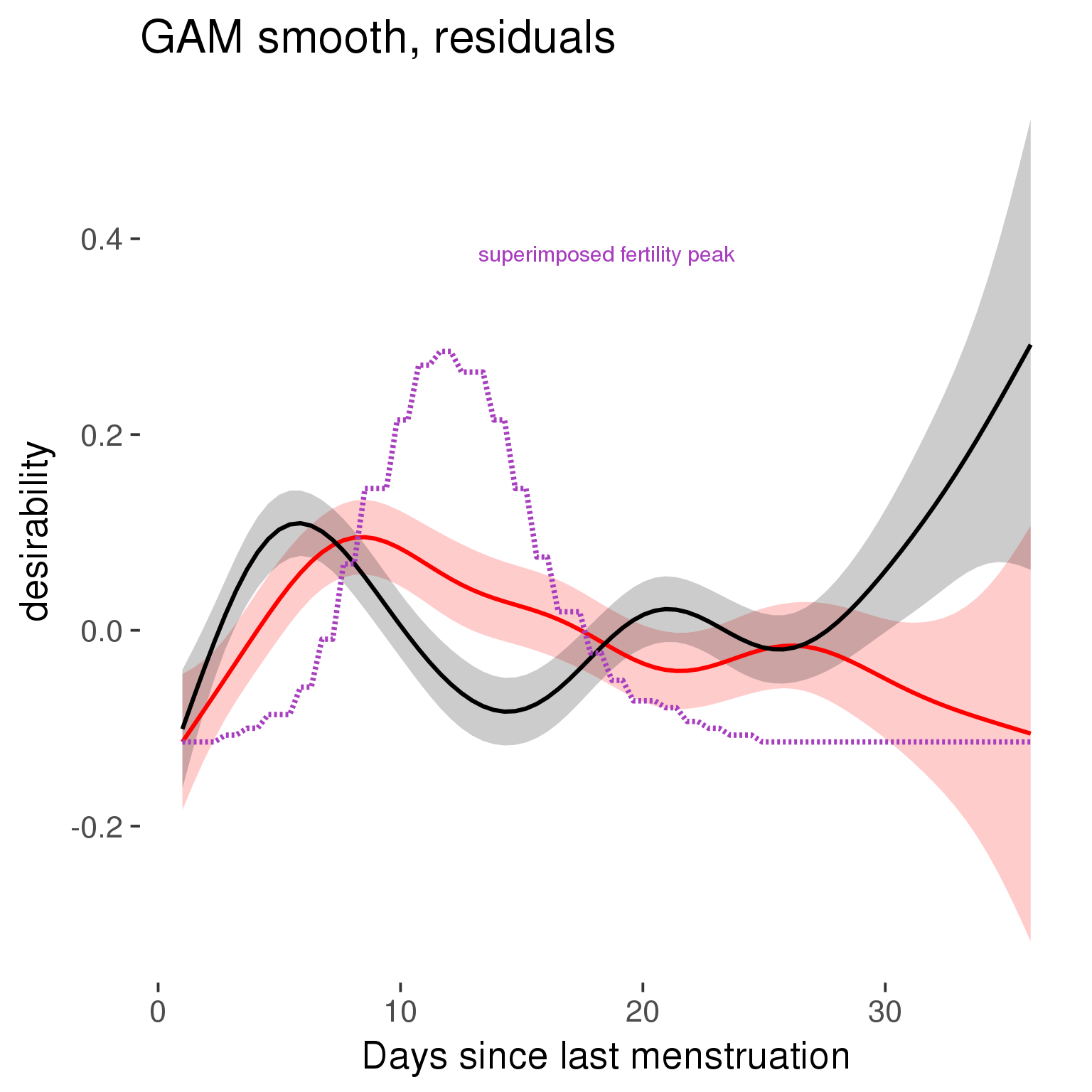
GAM smooth on raw data
As before, but without partialling anything out.
tryCatch({
trend_plot = ggplot(tmp,aes_string(x = "RCD", y = outcome, colour = "included")) +
stat_smooth(geom = 'smooth',size = 0.8, fill = "#9ECAE1", method = 'gam', formula = y ~ s(x))
}, error = function(e){cat_message(e, "danger")})
tryCatch({
trend_data = ggplot_build(trend_plot)$data[[1]]
}, error = function(e){cat_message(e, "danger")})
trend_data$RCD = round(trend_data$x)
trend_data = left_join(trend_data, tmp %>% select(real, RCD,fertile) %>% unique(), by = "RCD")
trend_data %>%
filter(real == TRUE) %>%
mutate(superimposed = ( ( (fertile - 0.01)/0.58) * (max(y)-min(y) ) ) + min(y) ) ->
trend_data
plot1b = ggplot(trend_data) +
geom_ribbon(aes(x = x, ymin = ymin, ymax = ymax, fill = factor(group)), alpha = 0.2) +
geom_line(aes(x = x, y = y, colour = factor(group)), size = 0.8, stat = "identity") +
scale_x_continuous(caption_x) +
geom_line(aes(x = x, y = superimposed), color = "#a83fbf", size = 1, linetype = 'dashed') +
annotate("text",x = mean(trend_data$x), y = max(trend_data$superimposed,na.rm=T) + 0.1, label = 'superimposed fertility peak', color = "#a83fbf") +
scale_y_continuous(outcome_label) +
ggtitle("GAM smooth, raw data") +
scale_color_manual("Contraception status",values = c("2"="black","1"= "red"), labels = c("2"="hormonally\ncontracepting","1"="cycling"), guide = F) +
scale_fill_manual("Contraception status",values = c("2"="black","1"= "red"), labels = c("2"="hormonally\ncontracepting","1"="cycling"), guide = F)
suppressWarnings(print(plot1b))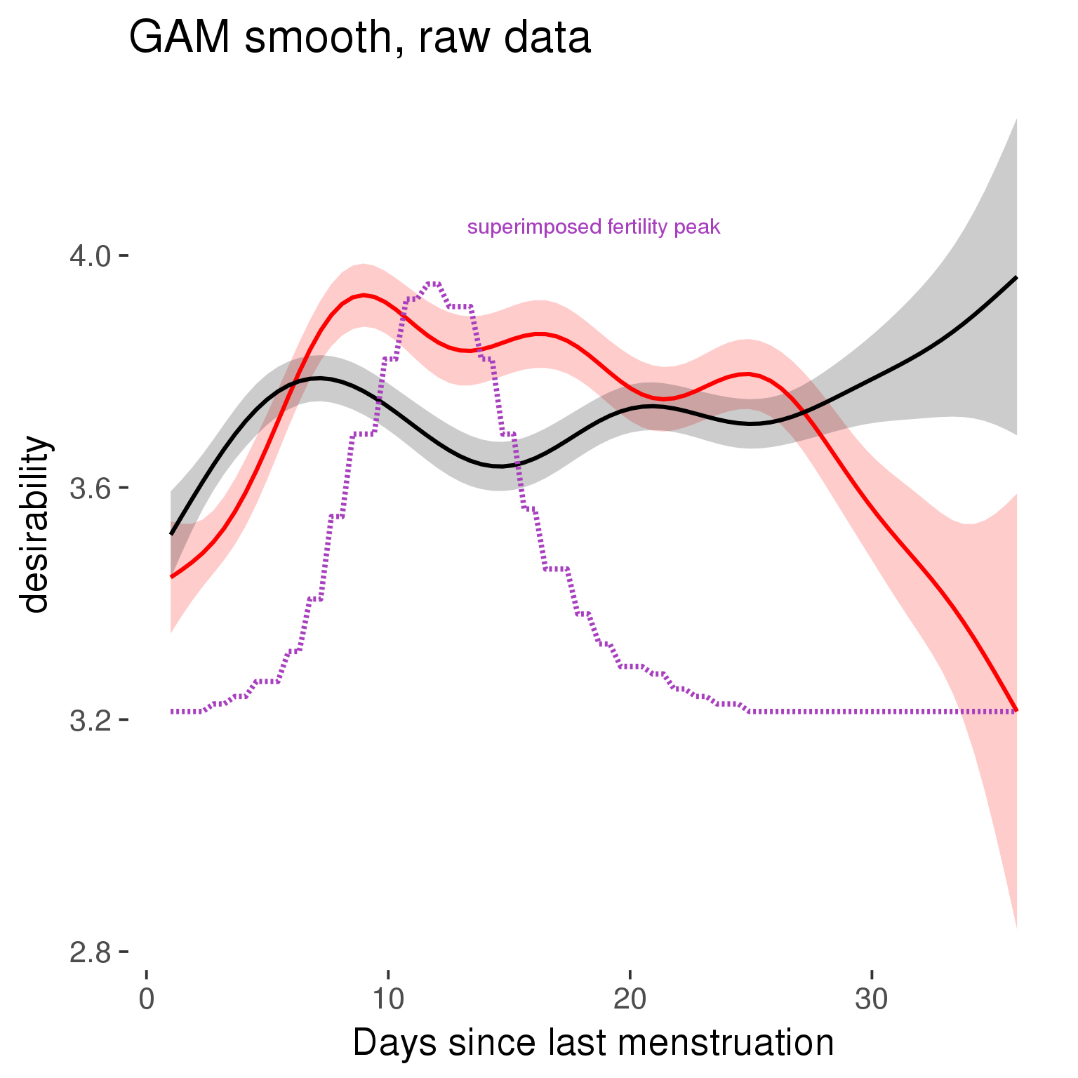
Means and standard errors over raw data
Nothing partialled out, just straight means with bootstrapped confidence intervals.
tryCatch({
trend_plot = ggplot(tmp,aes_string(x = "RCD", y = outcome, colour = "included")) +
geom_pointrange(size = 0.8, stat = 'summary', fun.data = "mean_cl_boot")
}, error = function(e){cat_message(e, "danger")})
tryCatch({
trend_data = ggplot_build(trend_plot)$data[[1]]
}, error = function(e){cat_message(e, "danger")})
trend_data$RCD = round(trend_data$x)
trend_data = left_join(trend_data, tmp %>% select(real, RCD,fertile) %>% unique(), by = "RCD")
trend_data %>%
filter(real == TRUE) %>%
mutate(superimposed = ( ( (fertile - 0.01)/0.58) * (max(y)-min(y) ) ) + min(y) ) ->
trend_data
plot3 = ggplot(trend_data) +
geom_pointrange(aes(x = x, y = y, ymin = ymin,ymax = ymax, colour = factor(group)), size = 0.8, stat = "identity", alpha = 0.6, position = position_dodge(width = .5)) +
scale_x_continuous("Days until next menstruation") +
geom_line(aes(x= x, y = superimposed), color = "#a83fbf", size = 1, linetype = 'dashed') +
annotate("text",x = mean(trend_data$x), y = max(trend_data$superimposed,na.rm=T) + 0.1, label = 'superimposed fertility peak', color = "#a83fbf") +
scale_y_continuous(outcome_label) +
ggtitle("Means with standard errors, raw data") +
scale_color_manual("Contraception status",values = c("2"="black","1"= "red"), labels = c("2"="hormonally\ncontracepting","1"="cycling"), guide = F) +
scale_fill_manual("Contraception status",values = c("2"="black","1"= "red"), labels = c("2"="hormonally\ncontracepting","1"="cycling"), guide = F)
suppressWarnings(print(plot3))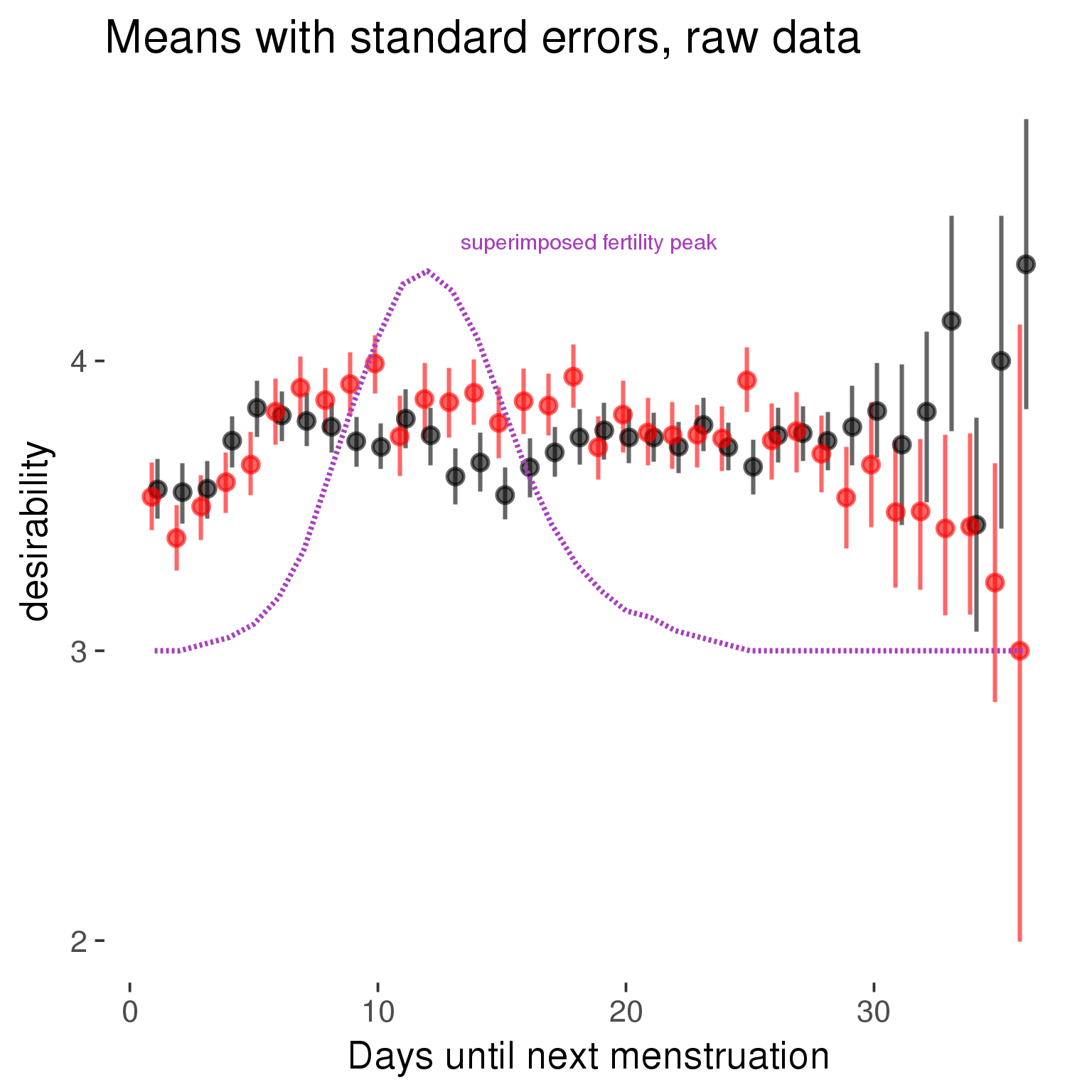
Cycle lengths from 27 to 30
Backward-counted
model %>%
plot_curve(diary %>% filter(minimum_cycle_length_diary <= 30, minimum_cycle_length_diary >= 27) %>% mutate(fertile=prc_stirn_b))outcome = names(model@frame)[1]
outcome_label = recode(str_replace_all(str_replace_all(str_replace_all(outcome, "_", " "), " pair", "-pair"), " 1", ""),
"desirability 1" = "self-perceived desirability",
"NARQ admiration" = "narcissistic admiration",
"NARQ rivalry" = "narcissistic rivalry",
"extra-pair" = "extra-pair desire & behaviour",
"had sexual intercourse" = "sexual intercourse")
library(ggplot2)
# form a subset and run the model without the hormonal contraception and the fertility predictors
tmp = diary %>%
filter(!is.na(fertile), !is.na(included),
RCD > -1 * minimum_cycle_length_diary, RCD > -40)
new_form = update.formula(formula(model), new = . ~ . - fertile * included)
tmp$residuals = residuals(update(model, new_form, data = tmp , na.action = na.exclude))
tmp = tmp %>%
filter(!is.na(RCD), !is.na(residuals))
rcd_min = min(tmp$RCD)
tmp$real = FALSE
tmp_before = tmp
tmp_before$RCD = tmp_before$RCD + min(tmp$RCD) - 1
tmp_after = tmp
tmp_after$RCD = tmp_after$RCD - min(tmp$RCD) + 1
tmp$real = TRUE
tmp = bind_rows(tmp_before %>% filter(RCD > rcd_min - 11), tmp, tmp_after %>% filter(RCD < 11))GAM smooth on residuals
Here, we partialled out menstruation and individual random effects, then superimposed estimated probability of being in the fertile window scaled to the range of the estimated means. To address the periodicity of the cycle, we prepended and appended ten days of the timeseries to the end and the beginning of the timeseries. We then estimated the GAM and cut off the appended subsets before plotting.
tryCatch({
trend_plot = ggplot(tmp,aes(x = RCD, y = residuals, colour = included)) +
stat_smooth(geom = 'smooth',size = 0.8, fill = "#9ECAE1", method = 'gam', formula = y ~ s(x))
}, error = function(e){cat_message(e, "danger")})
tryCatch({
trend_data = ggplot_build(trend_plot)$data[[1]]
}, error = function(e){cat_message(e, "danger")})
trend_data$RCD = round(trend_data$x)
trend_data = left_join(trend_data, tmp %>% select(real, RCD,fertile) %>% unique(), by = "RCD")
trend_data %>%
filter(real == TRUE) %>%
mutate(superimposed = ( ( (fertile - 0.01)/0.58) * (max(y)-min(y) ) ) + min(y) ) ->
trend_data
ggplot(trend_data) +
geom_ribbon(aes(x = x, ymin = ymin, ymax = ymax, fill = factor(group)), alpha = 0.2) +
geom_line(aes(x = x, y = y, colour = factor(group)), size = 0.8, stat = "identity") +
scale_x_continuous(caption_x) +
geom_line(aes(x = x, y = superimposed), color = "#a83fbf", size = 1, linetype = 'dashed') +
annotate("text",x = mean(trend_data$x), y = max(trend_data$superimposed,na.rm=T) + 0.1, label = 'superimposed fertility peak', color = "#a83fbf") +
scale_y_continuous(outcome_label) +
ggtitle("GAM smooth, residuals") +
scale_color_manual("Contraception status",values = c("2"="black","1"= "red"), labels = c("2"="hormonally\ncontracepting","1"="cycling"), guide = F) +
scale_fill_manual("Contraception status",values = c("2"="black","1"= "red"), labels = c("2"="hormonally\ncontracepting","1"="cycling"), guide = F)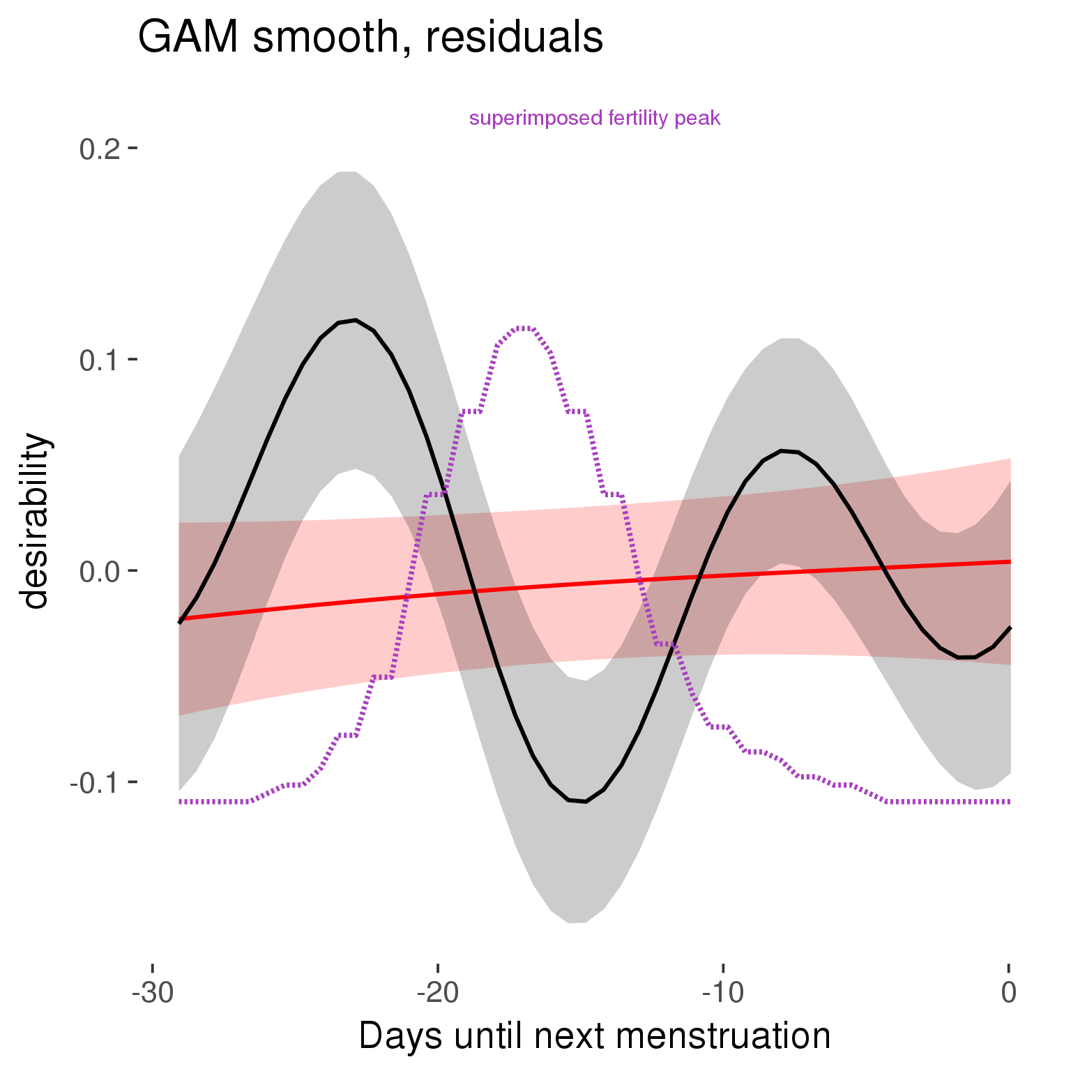
GAM smooth on raw data
As before, but without partialling anything out.
tryCatch({
trend_plot = ggplot(tmp,aes_string(x = "RCD", y = outcome, colour = "included")) +
stat_smooth(geom = 'smooth',size = 0.8, fill = "#9ECAE1", method = 'gam', formula = y ~ s(x))
}, error = function(e){cat_message(e, "danger")})
tryCatch({
trend_data = ggplot_build(trend_plot)$data[[1]]
}, error = function(e){cat_message(e, "danger")})
trend_data$RCD = round(trend_data$x)
trend_data = left_join(trend_data, tmp %>% select(real, RCD,fertile) %>% unique(), by = "RCD")
trend_data %>%
filter(real == TRUE) %>%
mutate(superimposed = ( ( (fertile - 0.01)/0.58) * (max(y)-min(y) ) ) + min(y) ) ->
trend_data
plot1b = ggplot(trend_data) +
geom_ribbon(aes(x = x, ymin = ymin, ymax = ymax, fill = factor(group)), alpha = 0.2) +
geom_line(aes(x = x, y = y, colour = factor(group)), size = 0.8, stat = "identity") +
scale_x_continuous(caption_x) +
geom_line(aes(x = x, y = superimposed), color = "#a83fbf", size = 1, linetype = 'dashed') +
annotate("text",x = mean(trend_data$x), y = max(trend_data$superimposed,na.rm=T) + 0.1, label = 'superimposed fertility peak', color = "#a83fbf") +
scale_y_continuous(outcome_label) +
ggtitle("GAM smooth, raw data") +
scale_color_manual("Contraception status",values = c("2"="black","1"= "red"), labels = c("2"="hormonally\ncontracepting","1"="cycling"), guide = F) +
scale_fill_manual("Contraception status",values = c("2"="black","1"= "red"), labels = c("2"="hormonally\ncontracepting","1"="cycling"), guide = F)
suppressWarnings(print(plot1b))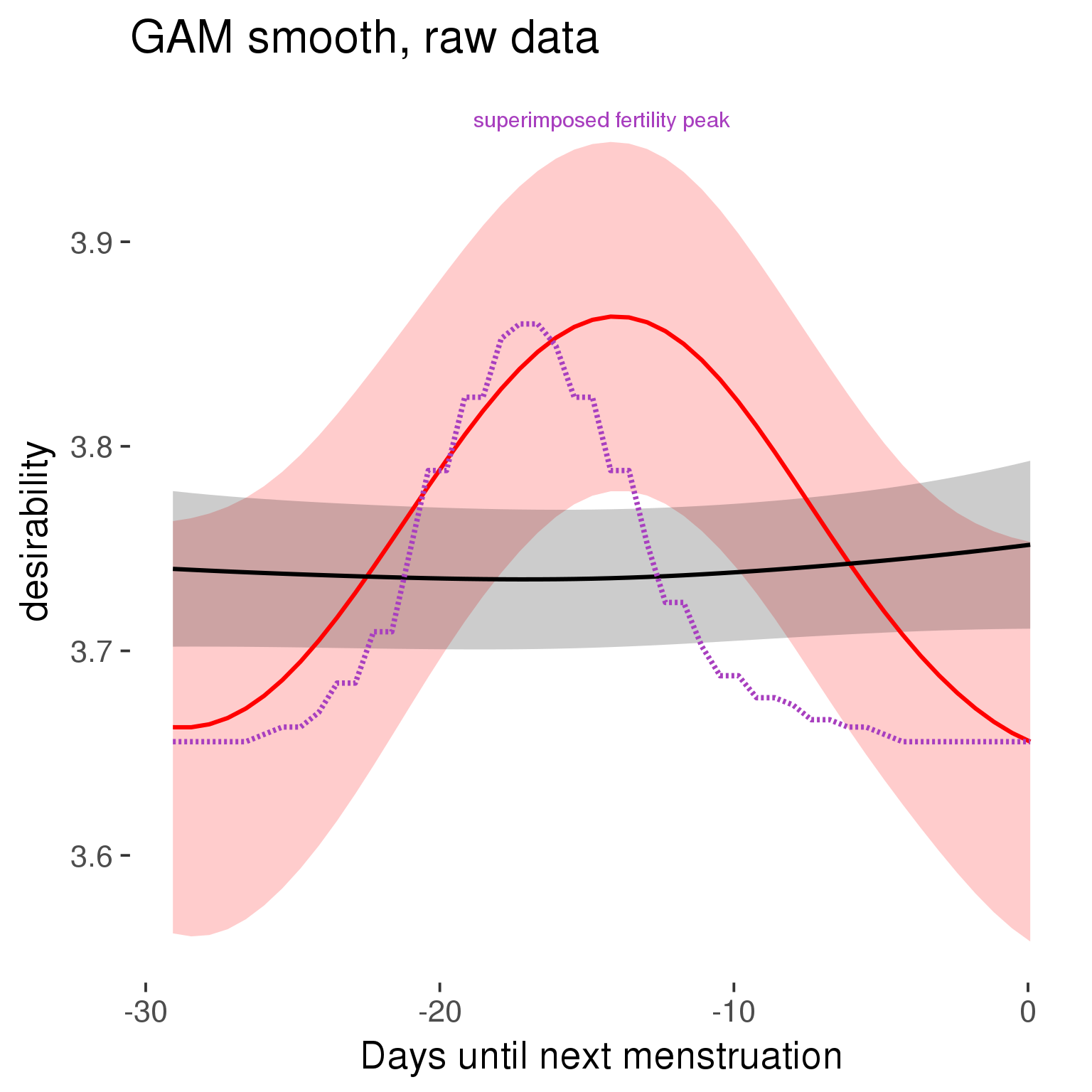
Means and standard errors over raw data
Nothing partialled out, just straight means with bootstrapped confidence intervals.
tryCatch({
trend_plot = ggplot(tmp,aes_string(x = "RCD", y = outcome, colour = "included")) +
geom_pointrange(size = 0.8, stat = 'summary', fun.data = "mean_cl_boot")
}, error = function(e){cat_message(e, "danger")})
tryCatch({
trend_data = ggplot_build(trend_plot)$data[[1]]
}, error = function(e){cat_message(e, "danger")})
trend_data$RCD = round(trend_data$x)
trend_data = left_join(trend_data, tmp %>% select(real, RCD,fertile) %>% unique(), by = "RCD")
trend_data %>%
filter(real == TRUE) %>%
mutate(superimposed = ( ( (fertile - 0.01)/0.58) * (max(y)-min(y) ) ) + min(y) ) ->
trend_data
plot3 = ggplot(trend_data) +
geom_pointrange(aes(x = x, y = y, ymin = ymin,ymax = ymax, colour = factor(group)), size = 0.8, stat = "identity", alpha = 0.6, position = position_dodge(width = .5)) +
scale_x_continuous("Days until next menstruation") +
geom_line(aes(x= x, y = superimposed), color = "#a83fbf", size = 1, linetype = 'dashed') +
annotate("text",x = mean(trend_data$x), y = max(trend_data$superimposed,na.rm=T) + 0.1, label = 'superimposed fertility peak', color = "#a83fbf") +
scale_y_continuous(outcome_label) +
ggtitle("Means with standard errors, raw data") +
scale_color_manual("Contraception status",values = c("2"="black","1"= "red"), labels = c("2"="hormonally\ncontracepting","1"="cycling"), guide = F) +
scale_fill_manual("Contraception status",values = c("2"="black","1"= "red"), labels = c("2"="hormonally\ncontracepting","1"="cycling"), guide = F)
suppressWarnings(print(plot3))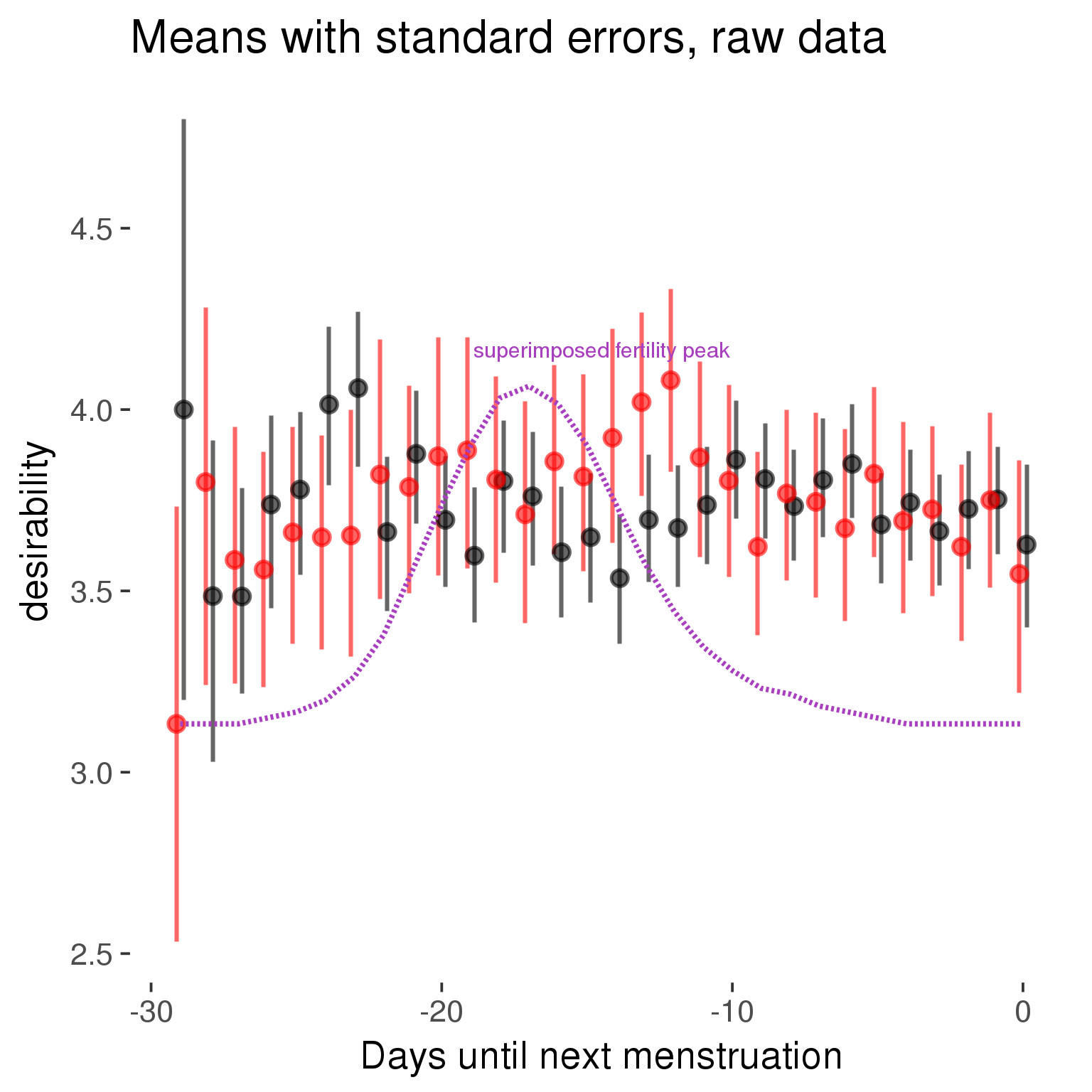
Forward-counted
model %>%
plot_curve(diary %>% filter(minimum_cycle_length_diary <= 30, minimum_cycle_length_diary >= 27) %>% mutate(RCD = FCD, fertile = prc_stirn_b_forward_counted), caption_x = "Days since last menstruation")outcome = names(model@frame)[1]
outcome_label = recode(str_replace_all(str_replace_all(str_replace_all(outcome, "_", " "), " pair", "-pair"), " 1", ""),
"desirability 1" = "self-perceived desirability",
"NARQ admiration" = "narcissistic admiration",
"NARQ rivalry" = "narcissistic rivalry",
"extra-pair" = "extra-pair desire & behaviour",
"had sexual intercourse" = "sexual intercourse")
library(ggplot2)
# form a subset and run the model without the hormonal contraception and the fertility predictors
tmp = diary %>%
filter(!is.na(fertile), !is.na(included),
RCD > -1 * minimum_cycle_length_diary, RCD > -40)
new_form = update.formula(formula(model), new = . ~ . - fertile * included)
tmp$residuals = residuals(update(model, new_form, data = tmp , na.action = na.exclude))
tmp = tmp %>%
filter(!is.na(RCD), !is.na(residuals))
rcd_min = min(tmp$RCD)
tmp$real = FALSE
tmp_before = tmp
tmp_before$RCD = tmp_before$RCD + min(tmp$RCD) - 1
tmp_after = tmp
tmp_after$RCD = tmp_after$RCD - min(tmp$RCD) + 1
tmp$real = TRUE
tmp = bind_rows(tmp_before %>% filter(RCD > rcd_min - 11), tmp, tmp_after %>% filter(RCD < 11))GAM smooth on residuals
Here, we partialled out menstruation and individual random effects, then superimposed estimated probability of being in the fertile window scaled to the range of the estimated means. To address the periodicity of the cycle, we prepended and appended ten days of the timeseries to the end and the beginning of the timeseries. We then estimated the GAM and cut off the appended subsets before plotting.
tryCatch({
trend_plot = ggplot(tmp,aes(x = RCD, y = residuals, colour = included)) +
stat_smooth(geom = 'smooth',size = 0.8, fill = "#9ECAE1", method = 'gam', formula = y ~ s(x))
}, error = function(e){cat_message(e, "danger")})
tryCatch({
trend_data = ggplot_build(trend_plot)$data[[1]]
}, error = function(e){cat_message(e, "danger")})
trend_data$RCD = round(trend_data$x)
trend_data = left_join(trend_data, tmp %>% select(real, RCD,fertile) %>% unique(), by = "RCD")
trend_data %>%
filter(real == TRUE) %>%
mutate(superimposed = ( ( (fertile - 0.01)/0.58) * (max(y)-min(y) ) ) + min(y) ) ->
trend_data
ggplot(trend_data) +
geom_ribbon(aes(x = x, ymin = ymin, ymax = ymax, fill = factor(group)), alpha = 0.2) +
geom_line(aes(x = x, y = y, colour = factor(group)), size = 0.8, stat = "identity") +
scale_x_continuous(caption_x) +
geom_line(aes(x = x, y = superimposed), color = "#a83fbf", size = 1, linetype = 'dashed') +
annotate("text",x = mean(trend_data$x), y = max(trend_data$superimposed,na.rm=T) + 0.1, label = 'superimposed fertility peak', color = "#a83fbf") +
scale_y_continuous(outcome_label) +
ggtitle("GAM smooth, residuals") +
scale_color_manual("Contraception status",values = c("2"="black","1"= "red"), labels = c("2"="hormonally\ncontracepting","1"="cycling"), guide = F) +
scale_fill_manual("Contraception status",values = c("2"="black","1"= "red"), labels = c("2"="hormonally\ncontracepting","1"="cycling"), guide = F)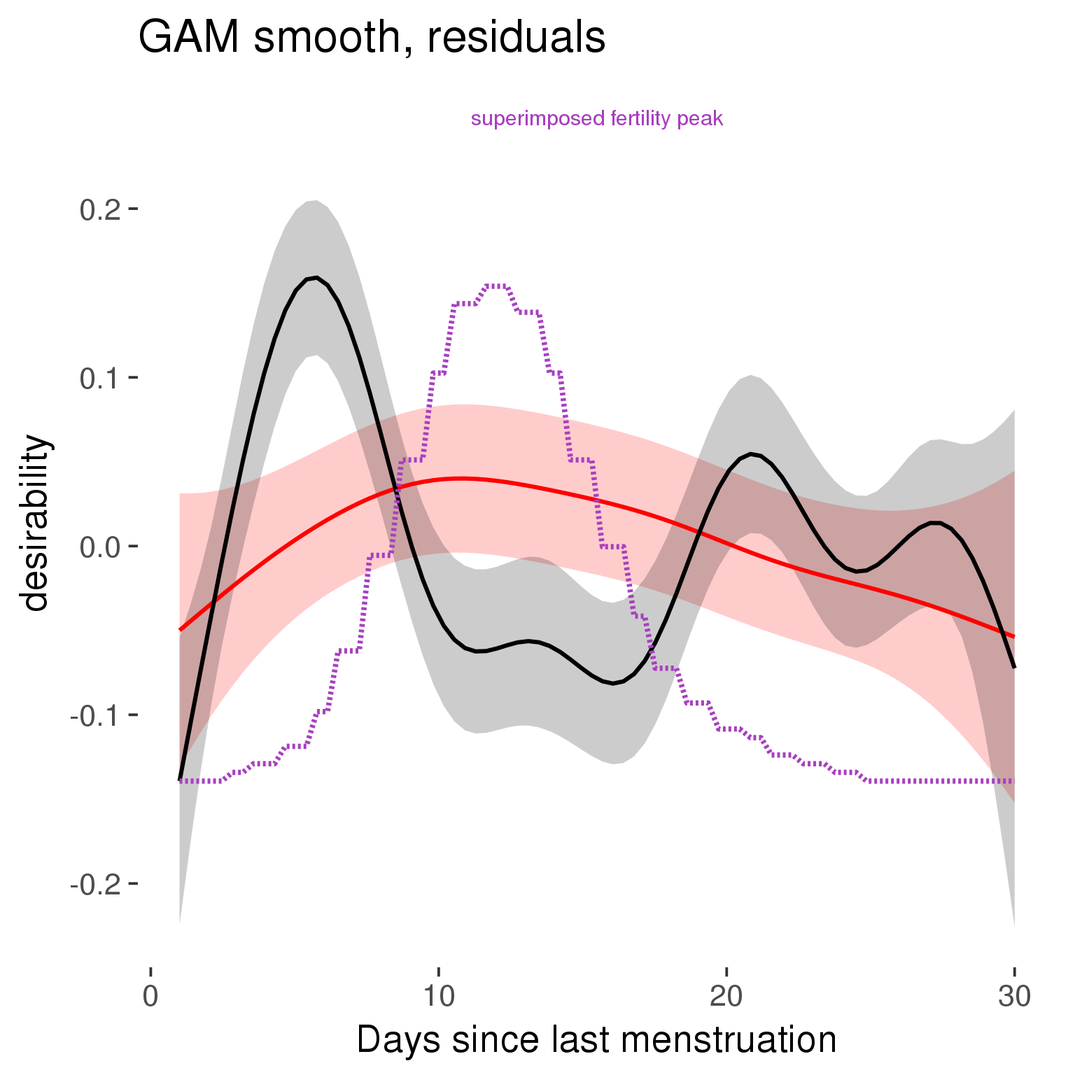
GAM smooth on raw data
As before, but without partialling anything out.
tryCatch({
trend_plot = ggplot(tmp,aes_string(x = "RCD", y = outcome, colour = "included")) +
stat_smooth(geom = 'smooth',size = 0.8, fill = "#9ECAE1", method = 'gam', formula = y ~ s(x))
}, error = function(e){cat_message(e, "danger")})
tryCatch({
trend_data = ggplot_build(trend_plot)$data[[1]]
}, error = function(e){cat_message(e, "danger")})
trend_data$RCD = round(trend_data$x)
trend_data = left_join(trend_data, tmp %>% select(real, RCD,fertile) %>% unique(), by = "RCD")
trend_data %>%
filter(real == TRUE) %>%
mutate(superimposed = ( ( (fertile - 0.01)/0.58) * (max(y)-min(y) ) ) + min(y) ) ->
trend_data
plot1b = ggplot(trend_data) +
geom_ribbon(aes(x = x, ymin = ymin, ymax = ymax, fill = factor(group)), alpha = 0.2) +
geom_line(aes(x = x, y = y, colour = factor(group)), size = 0.8, stat = "identity") +
scale_x_continuous(caption_x) +
geom_line(aes(x = x, y = superimposed), color = "#a83fbf", size = 1, linetype = 'dashed') +
annotate("text",x = mean(trend_data$x), y = max(trend_data$superimposed,na.rm=T) + 0.1, label = 'superimposed fertility peak', color = "#a83fbf") +
scale_y_continuous(outcome_label) +
ggtitle("GAM smooth, raw data") +
scale_color_manual("Contraception status",values = c("2"="black","1"= "red"), labels = c("2"="hormonally\ncontracepting","1"="cycling"), guide = F) +
scale_fill_manual("Contraception status",values = c("2"="black","1"= "red"), labels = c("2"="hormonally\ncontracepting","1"="cycling"), guide = F)
suppressWarnings(print(plot1b))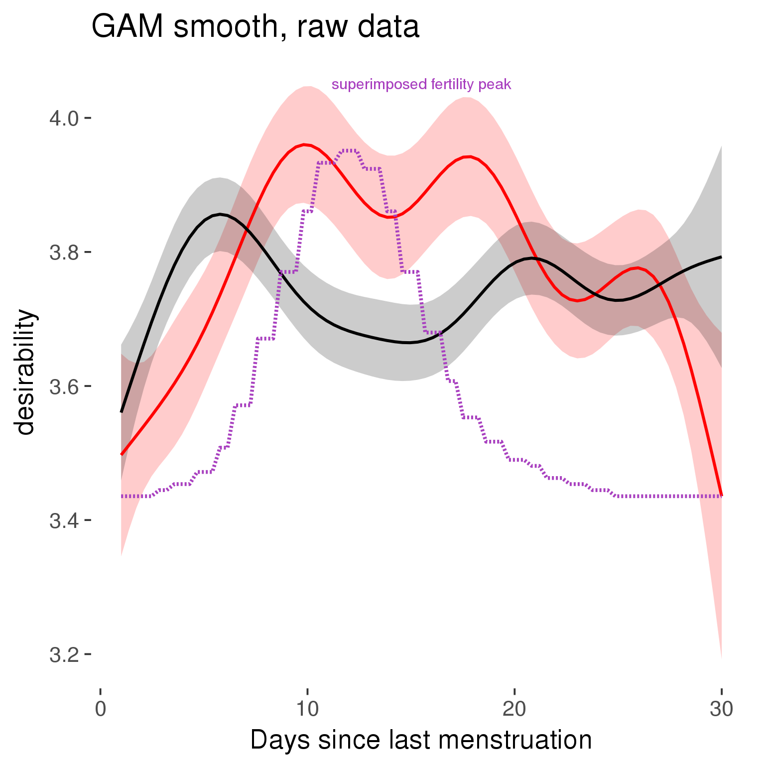
Means and standard errors over raw data
Nothing partialled out, just straight means with bootstrapped confidence intervals.
tryCatch({
trend_plot = ggplot(tmp,aes_string(x = "RCD", y = outcome, colour = "included")) +
geom_pointrange(size = 0.8, stat = 'summary', fun.data = "mean_cl_boot")
}, error = function(e){cat_message(e, "danger")})
tryCatch({
trend_data = ggplot_build(trend_plot)$data[[1]]
}, error = function(e){cat_message(e, "danger")})
trend_data$RCD = round(trend_data$x)
trend_data = left_join(trend_data, tmp %>% select(real, RCD,fertile) %>% unique(), by = "RCD")
trend_data %>%
filter(real == TRUE) %>%
mutate(superimposed = ( ( (fertile - 0.01)/0.58) * (max(y)-min(y) ) ) + min(y) ) ->
trend_data
plot3 = ggplot(trend_data) +
geom_pointrange(aes(x = x, y = y, ymin = ymin,ymax = ymax, colour = factor(group)), size = 0.8, stat = "identity", alpha = 0.6, position = position_dodge(width = .5)) +
scale_x_continuous("Days until next menstruation") +
geom_line(aes(x= x, y = superimposed), color = "#a83fbf", size = 1, linetype = 'dashed') +
annotate("text",x = mean(trend_data$x), y = max(trend_data$superimposed,na.rm=T) + 0.1, label = 'superimposed fertility peak', color = "#a83fbf") +
scale_y_continuous(outcome_label) +
ggtitle("Means with standard errors, raw data") +
scale_color_manual("Contraception status",values = c("2"="black","1"= "red"), labels = c("2"="hormonally\ncontracepting","1"="cycling"), guide = F) +
scale_fill_manual("Contraception status",values = c("2"="black","1"= "red"), labels = c("2"="hormonally\ncontracepting","1"="cycling"), guide = F)
suppressWarnings(print(plot3))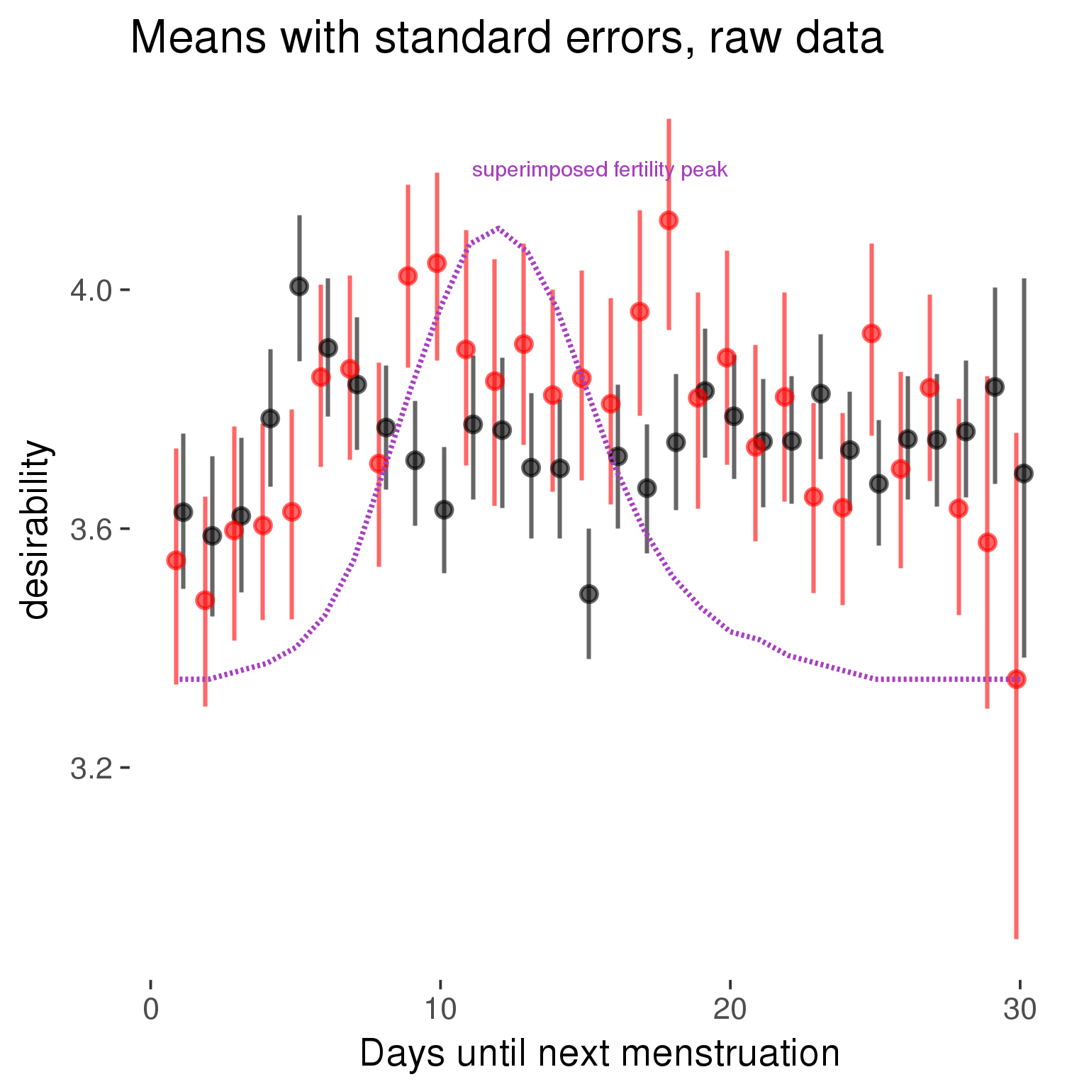
Robustness checks
M_r1: Random slopes for conception risk and menstruation
tryCatch({
# refit model with random effects for fertile and menstruation dummies
with_ind_diff = update(model, formula = . ~ . - (1| person) + (1 + fertile + menstruation | person))
# pull the random effects, format as tibble
rand = coef(with_ind_diff)$person %>%
tibble::rownames_to_column("person") %>%
mutate(person = as.numeric(person))
# pull the fixed effects
fixd = data.frame(fixef(with_ind_diff)) %>%
tibble::rownames_to_column("effect")
names(fixd) = c("effect", "pop_effect_size")
# pull apart the coefficients so that we can account for the fact that the random effect variation implicitly includes HC explaining the mean population-level effect of fertile/menstruation dummies among HC users
fixd = fixd %>%
separate(effect, c("included", "effect"), sep = ":", fill = "left") %>%
mutate(included = if_else(is.na(included), "cycling", str_replace(included, "included", "")))
fixd[2,c("included", "effect")] = c("horm_contra", "(Intercept)")
rand = rand %>%
# merge diary data on the random effects, so that we know who is a HC users and who isn't
inner_join(diary %>% select(person, included) %>% unique(), by = 'person') %>%
# gather into long format, to have the dataset by predictor
gather(effect, value, -person, -included) %>%
inner_join(fixd, by = c('effect', 'included')) %>%
# pull the fixed effects
mutate(
# only for those who are HC users, add the moderated population effect size for this effect (the random effects have the reference category mean)
value = if_else(included == "horm_contra", value + pop_effect_size, value),
effect = recode(effect, "includedhorm_contra" = "HC user",
"includedhorm_contra:fertile" = "HC user x fertile",
"includedhorm_contra:menstruationpre" = "HC user x premens.",
"includedhorm_contra:menstruationyes" = "HC user x mens.",
"menstruationyes" = "mens.",
"menstruationpre" = "premens.")) %>%
group_by(included, effect) %>%
# filter out predictors that aren't modelled as varying/random
filter(sd(value) > 0)
# plot dot plot of random effects
print(
ggplot(rand, aes(x = included, y = value, color = included, fill = included)) +
facet_wrap( ~ effect, scales = "free") +
# geom_violin(alpha = 0.4, size = 0) +
geom_dotplot(binaxis='y', dotsize = 0.1, method = "histodot") +
# geom_jitter(alpha = 0.05) +
coord_flip() +
geom_pointrange(stat = 'summary', fun.data = 'mean_sdl', color = 'darkred', size = 1.2) +
scale_color_manual("Contraception status", values = c("horm_contra"="black","cycling"= "red"), labels = c("horm_contra"="hormonally\ncontracepting","cycling"="cycling"), guide = F) +
scale_fill_manual("Contraception status", values = c("horm_contra"="black","cycling"= "red"), labels = c("horm_contra"="hormonally\ncontracepting","1"="cycling"), guide = F) +
ggtitle("M_r1: allowing participant-varying slopes", subtitle = "for the conception risk measure and the menstruation dummies") +
scale_x_discrete("Hormonal contraception", breaks = c("horm_contra", "cycling"), labels = c("yes", "no")) +
scale_y_continuous("Random effect size distribution"))
print_summary(with_ind_diff)
cat(pander(anova(model, with_ind_diff)))
}, error = function(e){
with_ind_diff = model
cat_message(e, "danger")
})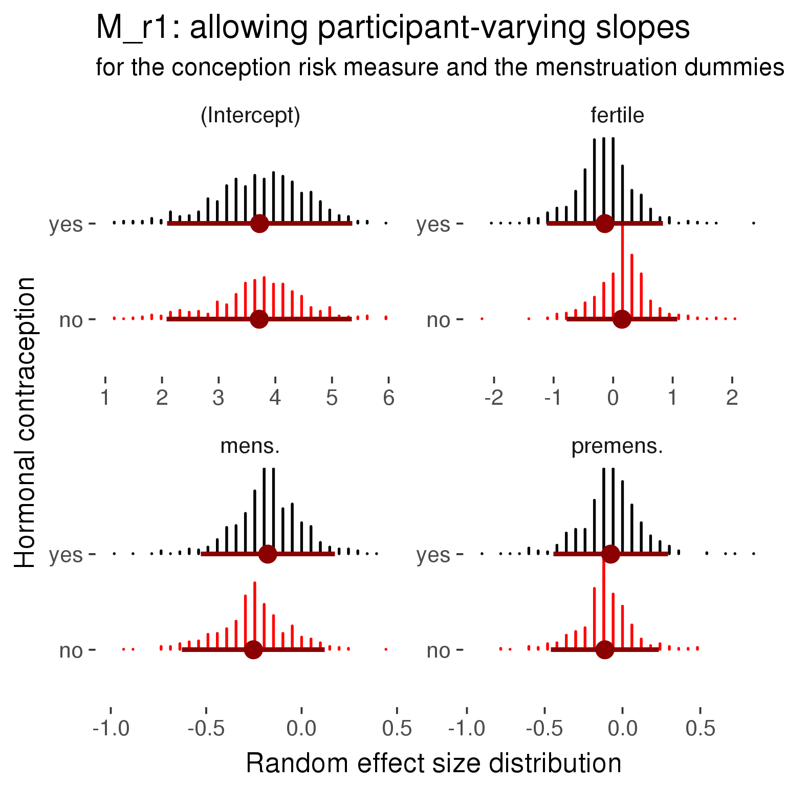
Linear mixed model fit by REML ['lmerMod']
Formula: desirability_1 ~ included + menstruation + fertile + fertile_mean +
(1 + fertile + menstruation | person) + included:menstruation + included:fertile
Data: diary
REML criterion at convergence: 84426
Scaled residuals:
Min 1Q Median 3Q Max
-4.140 -0.611 0.027 0.646 3.629
Random effects:
Groups Name Variance Std.Dev. Corr
person (Intercept) 0.796 0.892
fertile 0.796 0.892 -0.28
menstruationpre 0.148 0.385 -0.16 0.34
menstruationyes 0.142 0.376 -0.20 0.14 0.34
Residual 1.205 1.098
Number of obs: 26685, groups: person, 1054
Fixed effects:
Estimate Std. Error t value
(Intercept) 3.71586 0.07716 48.2
includedhorm_contra 0.00631 0.06449 0.1
menstruationpre -0.11330 0.04053 -2.8
menstruationyes -0.25265 0.03848 -6.6
fertile 0.14810 0.08499 1.7
fertile_mean -0.00751 0.35129 0.0
includedhorm_contra:menstruationpre 0.03745 0.05202 0.7
includedhorm_contra:menstruationyes 0.07512 0.05018 1.5
includedhorm_contra:fertile -0.28685 0.10786 -2.7
Correlation of Fixed Effects:
(Intr) incld_ mnstrtnp mnstrtny fertil frtl_m inclddhrm_cntr:mnstrtnp
inclddhrm_c -0.484
menstrutnpr -0.191 0.237
menstrutnys -0.207 0.246 0.374
fertile -0.209 0.327 0.416 0.307
fertile_men -0.760 -0.027 -0.008 0.002 -0.082
inclddhrm_cntr:mnstrtnp 0.158 -0.298 -0.779 -0.291 -0.323 -0.005
inclddhrm_cntr:mnstrtny 0.163 -0.306 -0.286 -0.767 -0.235 -0.007 0.363
inclddhrm_cntr:f 0.205 -0.415 -0.327 -0.242 -0.784 0.012 0.416
inclddhrm_cntr:mnstrtny
inclddhrm_c
menstrutnpr
menstrutnys
fertile
fertile_men
inclddhrm_cntr:mnstrtnp
inclddhrm_cntr:mnstrtny
inclddhrm_cntr:f 0.303
refitting model(s) with ML (instead of REML)
| Df | AIC | BIC | logLik | deviance | Chisq | Chi Df | Pr(>Chisq) | |
|---|---|---|---|---|---|---|---|---|
| object | 11 | 84649 | 84739 | -42313 | 84627 | NA | NA | NA |
| ..1 | 20 | 84430 | 84594 | -42195 | 84390 | 236.5 | 9 | 6.882e-46 |
robustness_check_ovu_shift(model, diary)M_e: Exclusion criteria
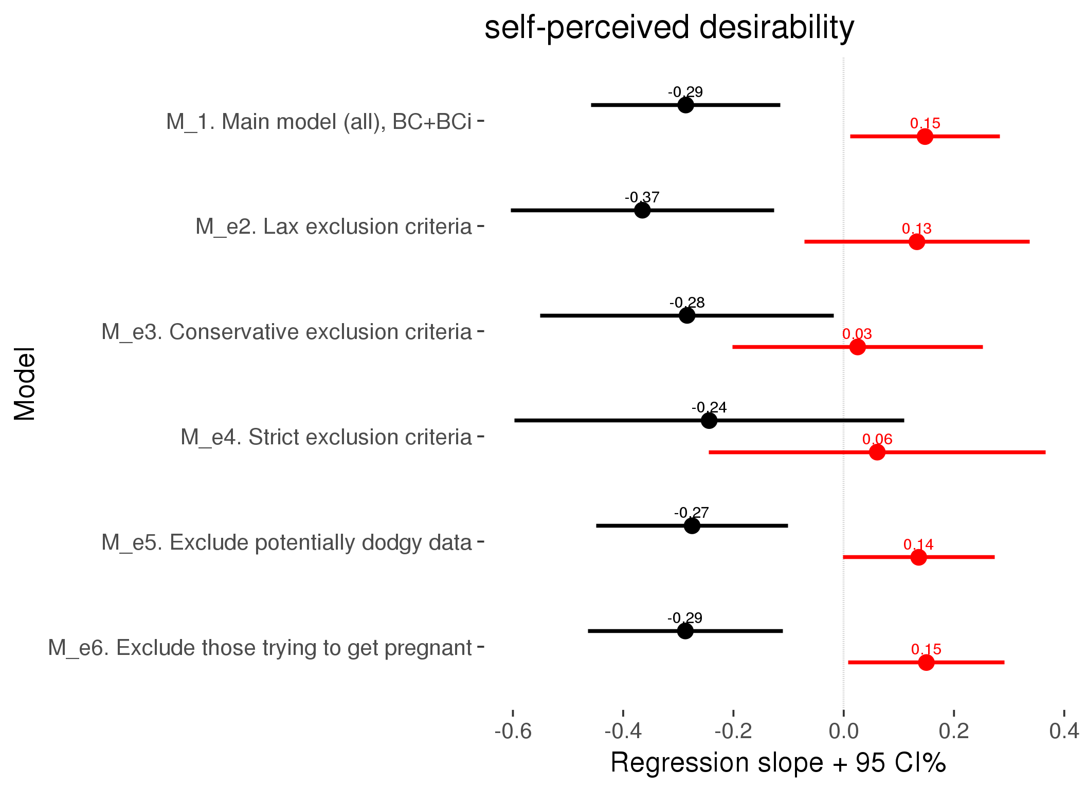
M_p: Predictors
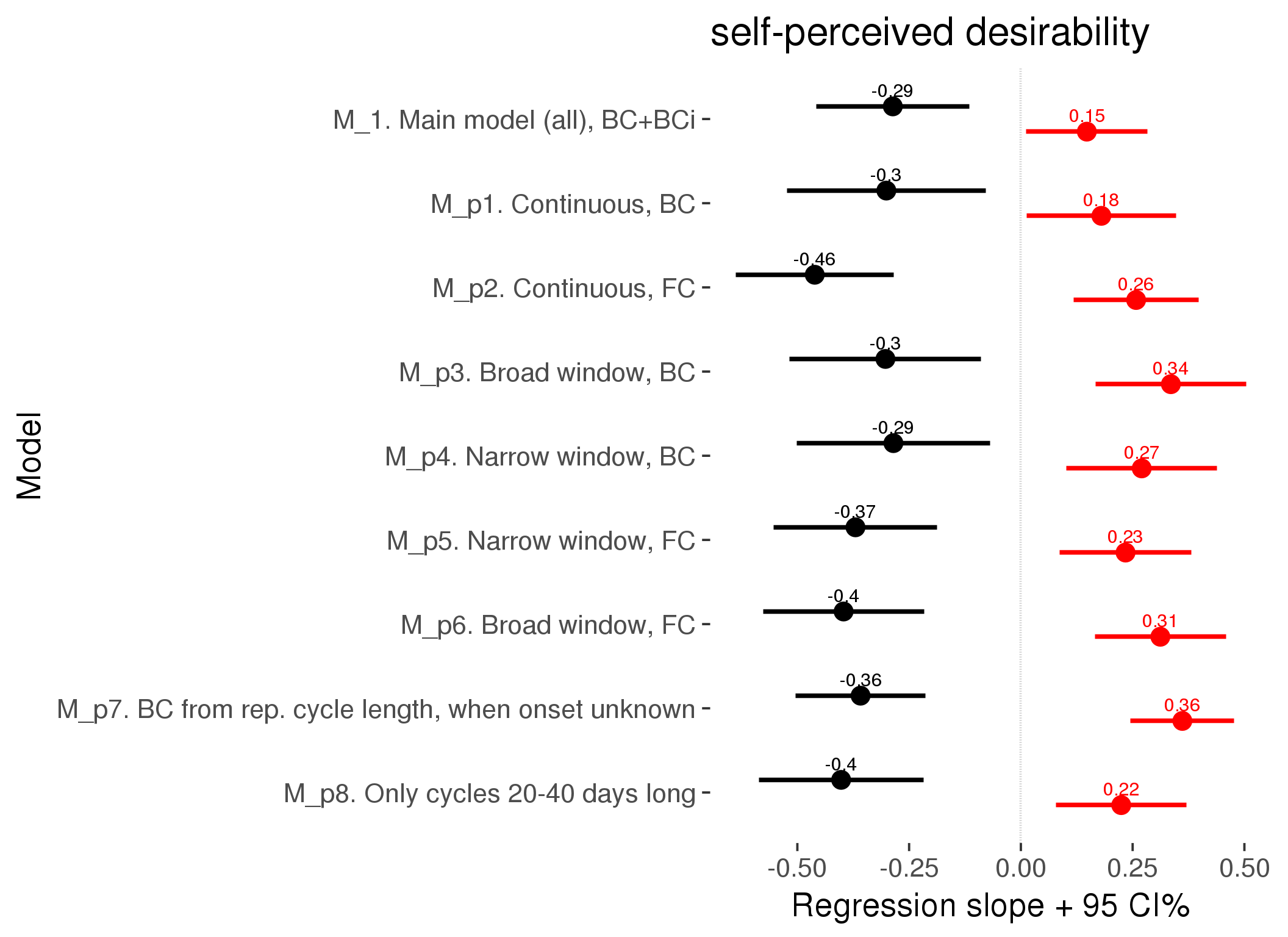
M_c: Covariates, controls, autocorrelation
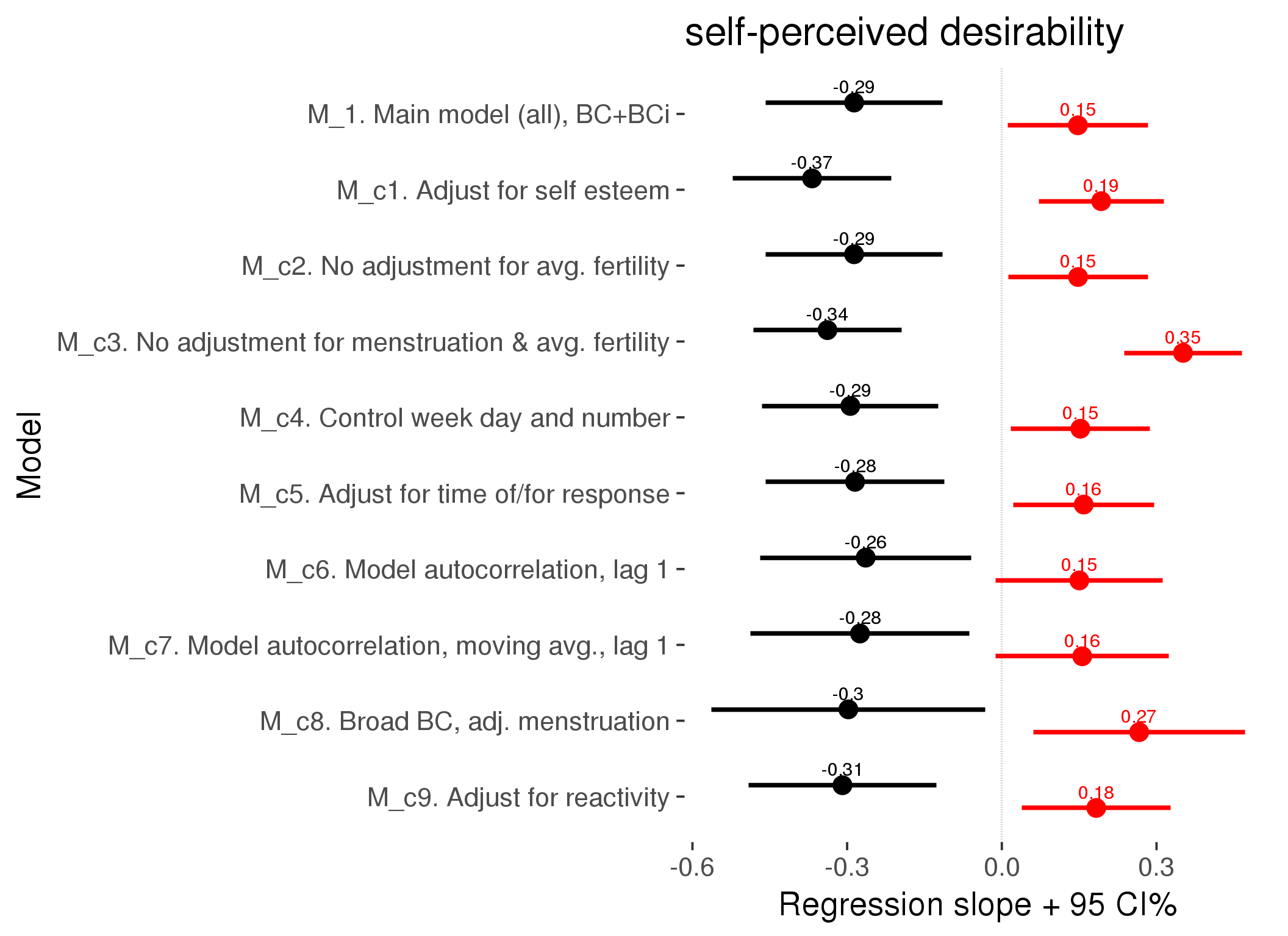
Linear mixed model fit by REML ['lmerMod']
REML criterion at convergence: 77305
Scaled residuals:
Min 1Q Median 3Q Max
-4.001 -0.627 0.027 0.664 3.811
Random effects:
Groups Name Variance Std.Dev.
person (Intercept) 0.7241 0.851
Xr.2 s(days_filled_out):includedhorm_contra 0.0000 0.000
Xr.1 s(days_filled_out):includedcycling 0.1038 0.322
Xr.0 s(day_number):includedhorm_contra 0.0000 0.000
Xr s(day_number):includedcycling 0.0747 0.273
Residual 1.2519 1.119
Number of obs: 24382, groups: person, 1054; Xr.2, 8; Xr.1, 8; Xr.0, 8; Xr, 8
Fixed effects:
Estimate Std. Error t value
X(Intercept) 3.6848 0.0763 48.3
Xincludedhorm_contra 0.0143 0.0630 0.2
Xmenstruationpre -0.1054 0.0357 -3.0
Xmenstruationyes -0.2404 0.0343 -7.0
Xfertile 0.1831 0.0735 2.5
Xfertile_mean 0.0223 0.3485 0.1
Xincludedhorm_contra:menstruationpre 0.0168 0.0457 0.4
Xincludedhorm_contra:menstruationyes 0.0668 0.0448 1.5
Xincludedhorm_contra:fertile -0.3091 0.0930 -3.3
Xs(day_number):includedcyclingFx1 -0.0202 0.1117 -0.2
Xs(day_number):includedhorm_contraFx1 0.1376 0.0484 2.8
Xs(days_filled_out):includedcyclingFx1 -0.1257 0.1208 -1.0
Xs(days_filled_out):includedhorm_contraFx1 -0.1539 0.0496 -3.1
Family: gaussian
Link function: identity
Formula:
desirability_1 ~ included + menstruation + fertile + fertile_mean +
s(day_number, by = included) + s(days_filled_out, by = included) +
included:menstruation + included:fertile
Parametric coefficients:
Estimate Std. Error t value Pr(>|t|)
(Intercept) 3.6848 0.0763 48.29 < 2e-16 ***
includedhorm_contra 0.0143 0.0630 0.23 0.82011
menstruationpre -0.1054 0.0357 -2.95 0.00315 **
menstruationyes -0.2404 0.0343 -7.01 2.4e-12 ***
fertile 0.1831 0.0735 2.49 0.01275 *
fertile_mean 0.0223 0.3485 0.06 0.94899
includedhorm_contra:menstruationpre 0.0168 0.0457 0.37 0.71359
includedhorm_contra:menstruationyes 0.0668 0.0448 1.49 0.13633
includedhorm_contra:fertile -0.3091 0.0930 -3.32 0.00089 ***
---
Signif. codes: 0 '***' 0.001 '**' 0.01 '*' 0.05 '.' 0.1 ' ' 1
Approximate significance of smooth terms:
edf Ref.df F p-value
s(day_number):includedcycling 3.10 3.10 1.58 0.1659
s(day_number):includedhorm_contra 1.00 1.00 8.07 0.0045 **
s(days_filled_out):includedcycling 3.49 3.49 1.04 0.2880
s(days_filled_out):includedhorm_contra 1.00 1.00 9.62 0.0019 **
---
Signif. codes: 0 '***' 0.001 '**' 0.01 '*' 0.05 '.' 0.1 ' ' 1
R-sq.(adj) = 0.000688
lmer.REML = 77305 Scale est. = 1.2519 n = 24382
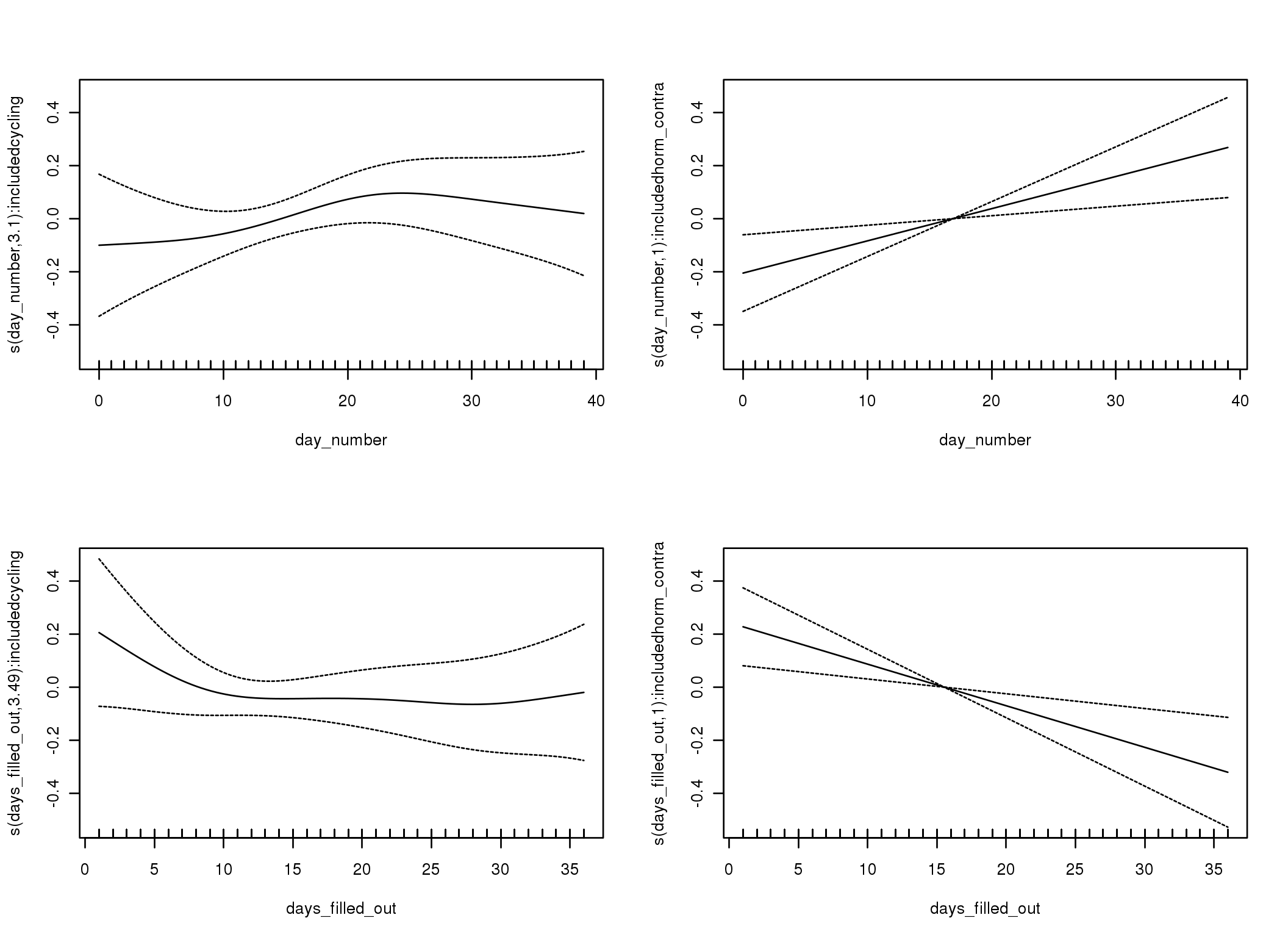
Linear mixed-effects model fit by REML
Data: diary
AIC BIC logLik
83366 83465 -41671
Random effects:
Formula: ~1 | person
(Intercept) Residual
StdDev: 0.8315 1.137
Correlation Structure: ARMA(1,0)
Formula: ~day_number | person
Parameter estimate(s):
Phi1
0.2633
Fixed effects: desirability_1 ~ included * (menstruation + fertile) + fertile_mean
Value Std.Error DF t-value p-value
(Intercept) 3.718 0.0770 25625 48.30 0.0000
includedhorm_contra 0.004 0.0634 1051 0.06 0.9548
menstruationpre -0.104 0.0392 25625 -2.66 0.0079
menstruationyes -0.239 0.0366 25625 -6.53 0.0000
fertile 0.150 0.0826 25625 1.82 0.0689
fertile_mean -0.009 0.3542 1051 -0.02 0.9802
includedhorm_contra:menstruationpre 0.041 0.0503 25625 0.82 0.4126
includedhorm_contra:menstruationyes 0.073 0.0478 25625 1.54 0.1241
includedhorm_contra:fertile -0.264 0.1045 25625 -2.53 0.0115
Correlation:
(Intr) incld_ mnstrtnp mnstrtny fertil frtl_m inclddhrm_cntr:mnstrtnp
includedhorm_contra -0.477
menstruationpre -0.195 0.244
menstruationyes -0.191 0.237 0.401
fertile -0.187 0.308 0.433 0.364
fertile_mean -0.768 -0.028 -0.007 -0.005 -0.084
includedhorm_contra:menstruationpre 0.160 -0.305 -0.779 -0.312 -0.336 -0.005
includedhorm_contra:menstruationyes 0.153 -0.290 -0.307 -0.766 -0.278 -0.004 0.386
includedhorm_contra:fertile 0.189 -0.390 -0.342 -0.288 -0.786 0.014 0.432
inclddhrm_cntr:mnstrtny
includedhorm_contra
menstruationpre
menstruationyes
fertile
fertile_mean
includedhorm_contra:menstruationpre
includedhorm_contra:menstruationyes
includedhorm_contra:fertile 0.358
Standardized Within-Group Residuals:
Min Q1 Med Q3 Max
-3.94515 -0.62888 0.03167 0.65770 3.52919
Number of Observations: 26685
Number of Groups: 1054
Linear mixed-effects model fit by REML
Data: diary
AIC BIC logLik
83278 83384 -41626
Random effects:
Formula: ~1 | person
(Intercept) Residual
StdDev: 0.8227 1.142
Correlation Structure: ARMA(1,1)
Formula: ~day_number | person
Parameter estimate(s):
Phi1 Theta1
0.5141 -0.2688
Fixed effects: desirability_1 ~ included * (menstruation + fertile) + fertile_mean
Value Std.Error DF t-value p-value
(Intercept) 3.713 0.0772 25625 48.12 0.0000
includedhorm_contra 0.007 0.0636 1051 0.11 0.9147
menstruationpre -0.093 0.0398 25625 -2.35 0.0190
menstruationyes -0.236 0.0374 25625 -6.31 0.0000
fertile 0.156 0.0857 25625 1.82 0.0688
fertile_mean 0.004 0.3553 1051 0.01 0.9906
includedhorm_contra:menstruationpre 0.034 0.0512 25625 0.66 0.5116
includedhorm_contra:menstruationyes 0.068 0.0487 25625 1.39 0.1640
includedhorm_contra:fertile -0.275 0.1083 25625 -2.54 0.0111
Correlation:
(Intr) incld_ mnstrtnp mnstrtny fertil frtl_m inclddhrm_cntr:mnstrtnp
includedhorm_contra -0.477
menstruationpre -0.197 0.245
menstruationyes -0.195 0.241 0.410
fertile -0.189 0.313 0.410 0.356
fertile_mean -0.767 -0.029 -0.006 -0.005 -0.088
includedhorm_contra:menstruationpre 0.161 -0.306 -0.778 -0.319 -0.318 -0.005
includedhorm_contra:menstruationyes 0.155 -0.295 -0.315 -0.768 -0.273 -0.004 0.396
includedhorm_contra:fertile 0.192 -0.396 -0.324 -0.281 -0.786 0.015 0.409
inclddhrm_cntr:mnstrtny
includedhorm_contra
menstruationpre
menstruationyes
fertile
fertile_mean
includedhorm_contra:menstruationpre
includedhorm_contra:menstruationyes
includedhorm_contra:fertile 0.350
Standardized Within-Group Residuals:
Min Q1 Med Q3 Max
-3.90577 -0.62887 0.03436 0.65521 3.46413
Number of Observations: 26685
Number of Groups: 1054
M_d: Other designs
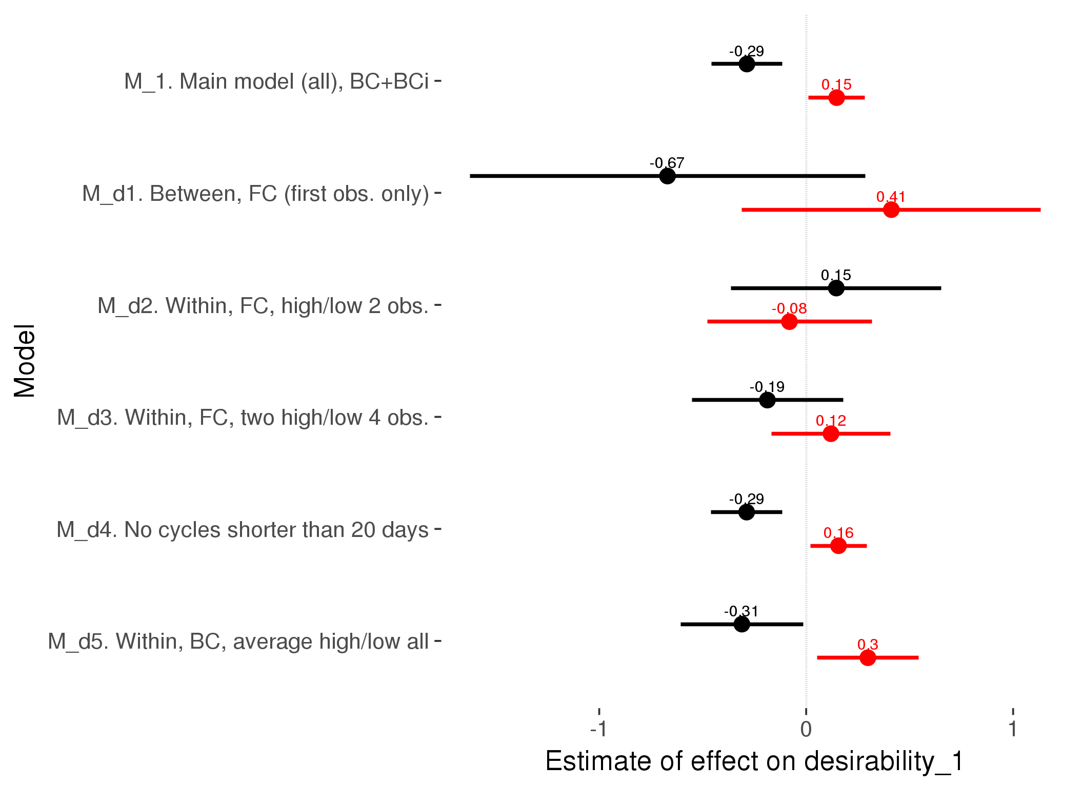
M_m1: Moderation by contraceptive method
Based on the sample with lax exclusion criteria. Users who used any hormonal contraception are classified as hormonal, users who use any awareness-based methods (counting, temperature-based) are classified as ‘fertility-awareness’, women who don’t fall into the before groups and use condoms, pessars, coitus interruptus etc. are classified as ‘barrie or abstinence’. Women who don’t use contraception or use other methods such as sterilisation are excluded from this analysis.
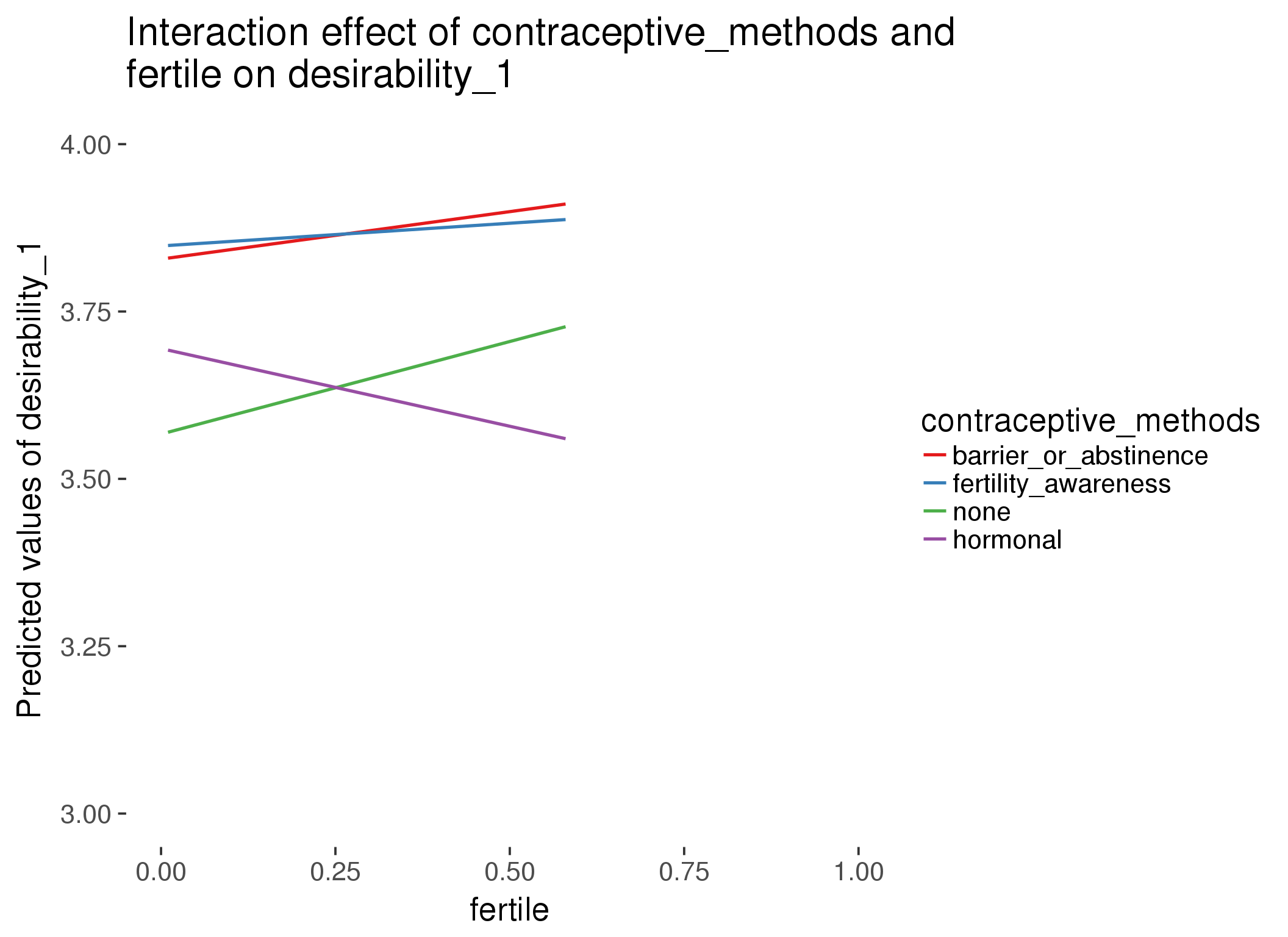
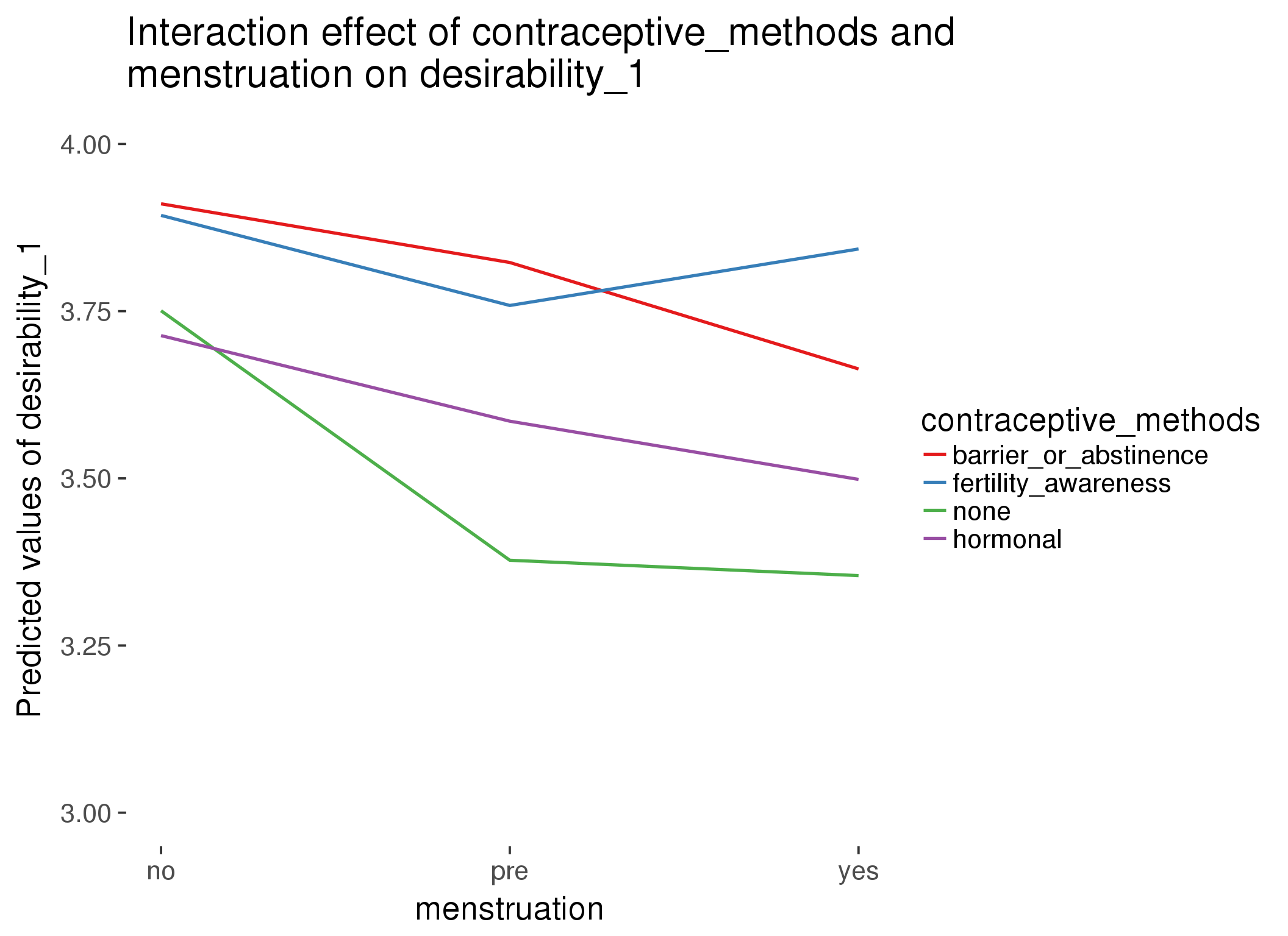
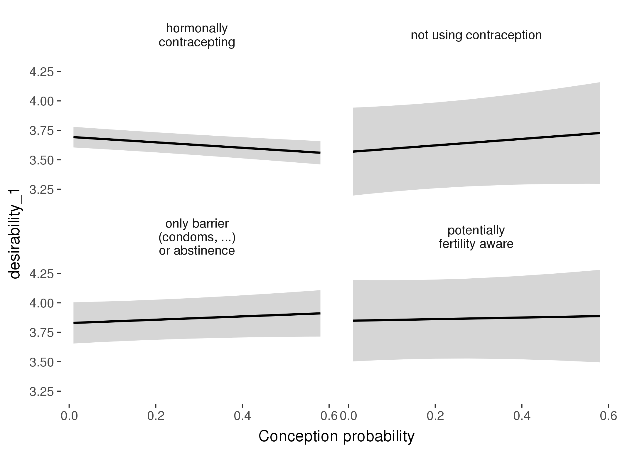
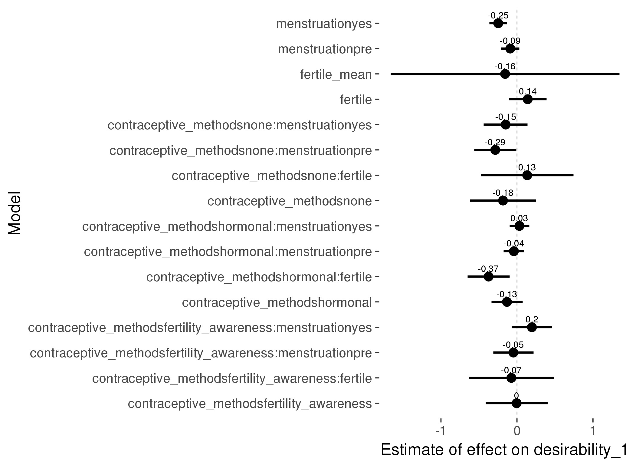
Linear mixed model fit by REML ['lmerMod']
Formula: desirability_1 ~ fertile_mean + (1 | person) + contraceptive_methods +
fertile + menstruation + fertile:contraceptive_methods + menstruation:contraceptive_methods
Data: diary
Subset: !is.na(included_lax) & contraceptive_method != "other"
REML criterion at convergence: 54029
Scaled residuals:
Min 1Q Median 3Q Max
-3.690 -0.636 0.026 0.664 3.608
Random effects:
Groups Name Variance Std.Dev.
person (Intercept) 0.663 0.814
Residual 1.280 1.131
Number of obs: 17029, groups: person, 513
Fixed effects:
Estimate Std. Error t value
(Intercept) 3.91300 0.15846 24.69
fertile_mean -0.15601 0.76802 -0.20
contraceptive_methodsfertility_awareness -0.00436 0.20806 -0.02
contraceptive_methodsnone -0.18353 0.22060 -0.83
contraceptive_methodshormonal -0.13147 0.10481 -1.25
fertile 0.14184 0.12614 1.12
menstruationpre -0.08777 0.06093 -1.44
menstruationyes -0.24694 0.05819 -4.24
contraceptive_methodsfertility_awareness:fertile -0.07389 0.28648 -0.26
contraceptive_methodsnone:fertile 0.13475 0.31017 0.43
contraceptive_methodshormonal:fertile -0.37400 0.14090 -2.65
contraceptive_methodsfertility_awareness:menstruationpre -0.04693 0.13498 -0.35
contraceptive_methodsnone:menstruationpre -0.28538 0.14109 -2.02
contraceptive_methodshormonal:menstruationpre -0.04023 0.06863 -0.59
contraceptive_methodsfertility_awareness:menstruationyes 0.19676 0.13564 1.45
contraceptive_methodsnone:menstruationyes -0.14919 0.14755 -1.01
contraceptive_methodshormonal:menstruationyes 0.03187 0.06636 0.48
refitting model(s) with ML (instead of REML)
| Df | AIC | BIC | logLik | deviance | Chisq | Chi Df | Pr(>Chisq) | |
|---|---|---|---|---|---|---|---|---|
| add_main | 13 | 54021 | 54121 | -26997 | 53995 | NA | NA | NA |
| by_method | 19 | 54021 | 54168 | -26992 | 53983 | 11.46 | 6 | 0.07529 |
M_m2: Moderation by participant age
model %>%
test_moderator("age_group", diary, xlevels = 5)refitting model(s) with ML (instead of REML)
| Df | AIC | BIC | logLik | deviance | Chisq | Chi Df | Pr(>Chisq) | |
|---|---|---|---|---|---|---|---|---|
| with_main | 19 | 84648 | 84803 | -42305 | 84610 | NA | NA | NA |
| with_mod | 27 | 84651 | 84872 | -42298 | 84597 | 12.82 | 8 | 0.1181 |
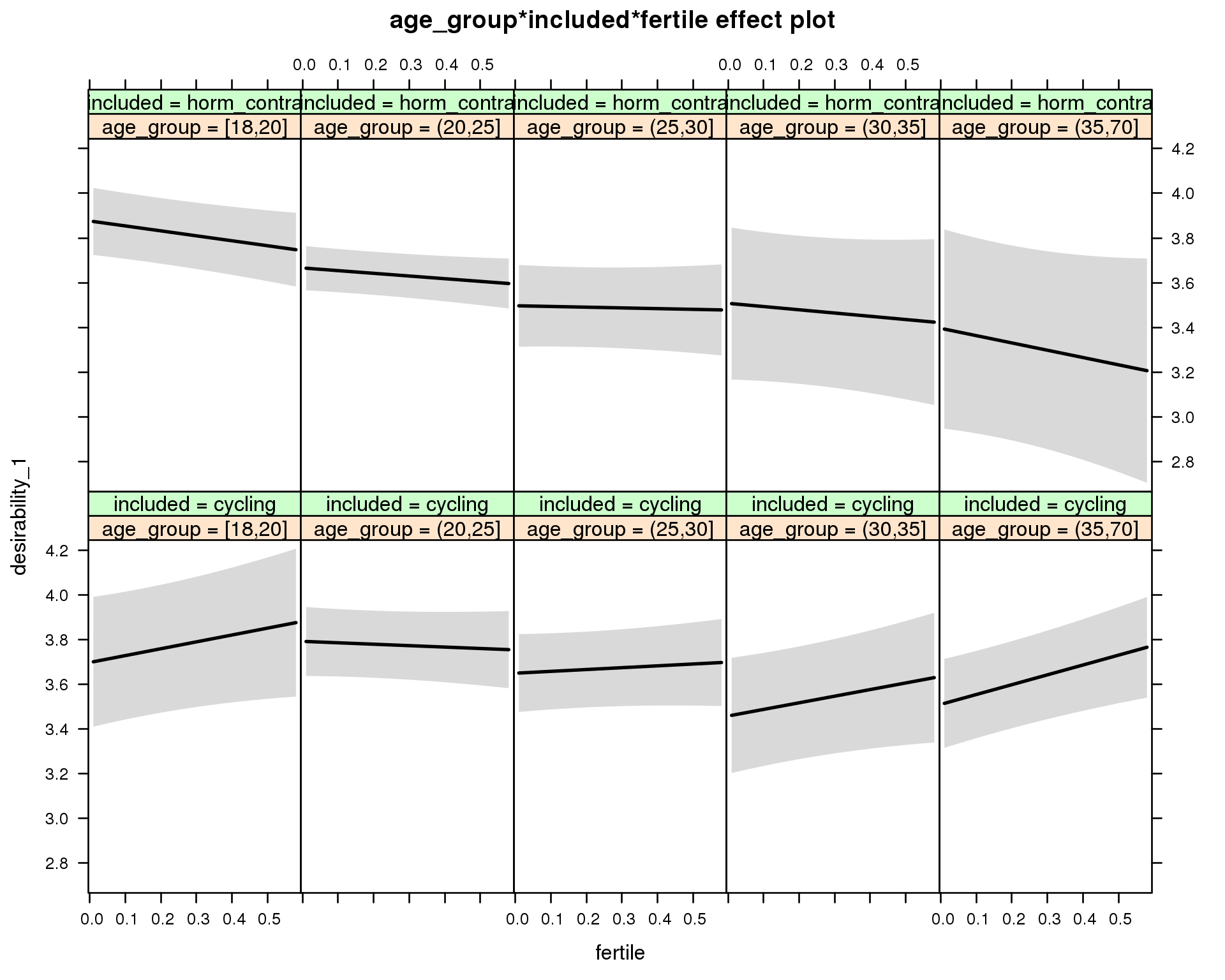
Linear mixed model fit by REML ['lmerMod']
Formula: desirability_1 ~ menstruation + fertile_mean + (1 | person) +
age_group + included + fertile + menstruation:included +
age_group:included + age_group:fertile + included:fertile + age_group:included:fertile
Data: diary
REML criterion at convergence: 84666
Scaled residuals:
Min 1Q Median 3Q Max
-4.061 -0.626 0.029 0.664 3.641
Random effects:
Groups Name Variance Std.Dev.
person (Intercept) 0.722 0.85
Residual 1.263 1.12
Number of obs: 26685, groups: person, 1054
Fixed effects:
Estimate Std. Error t value
(Intercept) 3.7580 0.1573 23.90
menstruationpre -0.1096 0.0343 -3.19
menstruationyes -0.2534 0.0323 -7.84
fertile_mean 0.0220 0.3488 0.06
age_group(20,25] 0.0944 0.1680 0.56
age_group(25,30] -0.0481 0.1729 -0.28
age_group(30,35] -0.2397 0.1984 -1.21
age_group(35,70] -0.1875 0.1796 -1.04
includedhorm_contra 0.1609 0.1684 0.96
fertile 0.3073 0.1979 1.55
menstruationpre:includedhorm_contra 0.0254 0.0440 0.58
menstruationyes:includedhorm_contra 0.0716 0.0424 1.69
age_group(20,25]:includedhorm_contra -0.3047 0.1914 -1.59
age_group(25,30]:includedhorm_contra -0.3313 0.2110 -1.57
age_group(30,35]:includedhorm_contra -0.1288 0.2745 -0.47
age_group(35,70]:includedhorm_contra -0.2931 0.3004 -0.98
age_group(20,25]:fertile -0.3712 0.2192 -1.69
age_group(25,30]:fertile -0.2249 0.2260 -1.00
age_group(30,35]:fertile -0.0111 0.2617 -0.04
age_group(35,70]:fertile 0.1332 0.2362 0.56
includedhorm_contra:fertile -0.5290 0.2195 -2.41
age_group(20,25]:includedhorm_contra:fertile 0.4727 0.2455 1.93
age_group(25,30]:includedhorm_contra:fertile 0.4143 0.2721 1.52
age_group(30,35]:includedhorm_contra:fertile 0.0875 0.3512 0.25
age_group(35,70]:includedhorm_contra:fertile -0.2382 0.3990 -0.60
M_m3: Moderation by weekend
model %>%
test_moderator("weekend", diary, xlevels = 2) refitting model(s) with ML (instead of REML)
| Df | AIC | BIC | logLik | deviance | Chisq | Chi Df | Pr(>Chisq) | |
|---|---|---|---|---|---|---|---|---|
| with_main | 13 | 84446 | 84553 | -42210 | 84420 | NA | NA | NA |
| with_mod | 15 | 84449 | 84572 | -42210 | 84419 | 1.075 | 2 | 0.5841 |
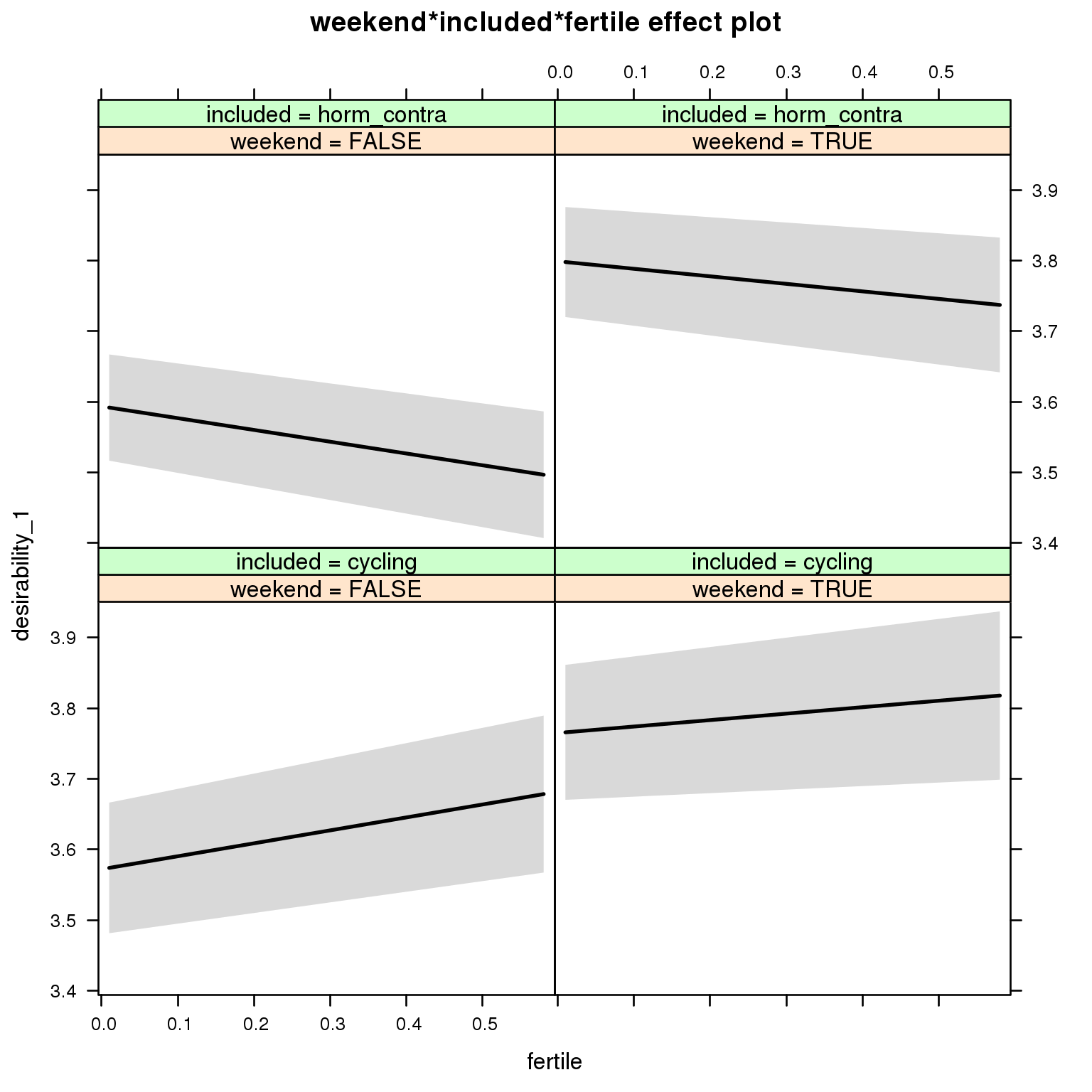
Linear mixed model fit by REML ['lmerMod']
Formula: desirability_1 ~ menstruation + fertile_mean + (1 | person) +
weekend + included + fertile + menstruation:included + weekend:included +
weekend:fertile + included:fertile + weekend:included:fertile
Data: diary
REML criterion at convergence: 84475
Scaled residuals:
Min 1Q Median 3Q Max
-4.010 -0.625 0.030 0.663 3.564
Random effects:
Groups Name Variance Std.Dev.
person (Intercept) 0.727 0.853
Residual 1.254 1.120
Number of obs: 26685, groups: person, 1054
Fixed effects:
Estimate Std. Error t value
(Intercept) 3.63153 0.07670 47.3
menstruationpre -0.11095 0.03416 -3.2
menstruationyes -0.25366 0.03218 -7.9
fertile_mean 0.02565 0.34804 0.1
weekendTRUE 0.19291 0.02978 6.5
includedhorm_contra 0.00376 0.06391 0.1
fertile 0.18338 0.08387 2.2
menstruationpre:includedhorm_contra 0.02604 0.04385 0.6
menstruationyes:includedhorm_contra 0.07502 0.04219 1.8
weekendTRUE:includedhorm_contra 0.01264 0.03833 0.3
weekendTRUE:fertile -0.09195 0.11550 -0.8
includedhorm_contra:fertile -0.35030 0.10654 -3.3
weekendTRUE:includedhorm_contra:fertile 0.15224 0.14690 1.0
M_m4: Moderation by weekday
model %>%
test_moderator("weekday", diary, xlevels = 7)refitting model(s) with ML (instead of REML)
| Df | AIC | BIC | logLik | deviance | Chisq | Chi Df | Pr(>Chisq) | |
|---|---|---|---|---|---|---|---|---|
| with_main | 23 | 84392 | 84580 | -42173 | 84346 | NA | NA | NA |
| with_mod | 35 | 84408 | 84694 | -42169 | 84338 | 8.196 | 12 | 0.7696 |
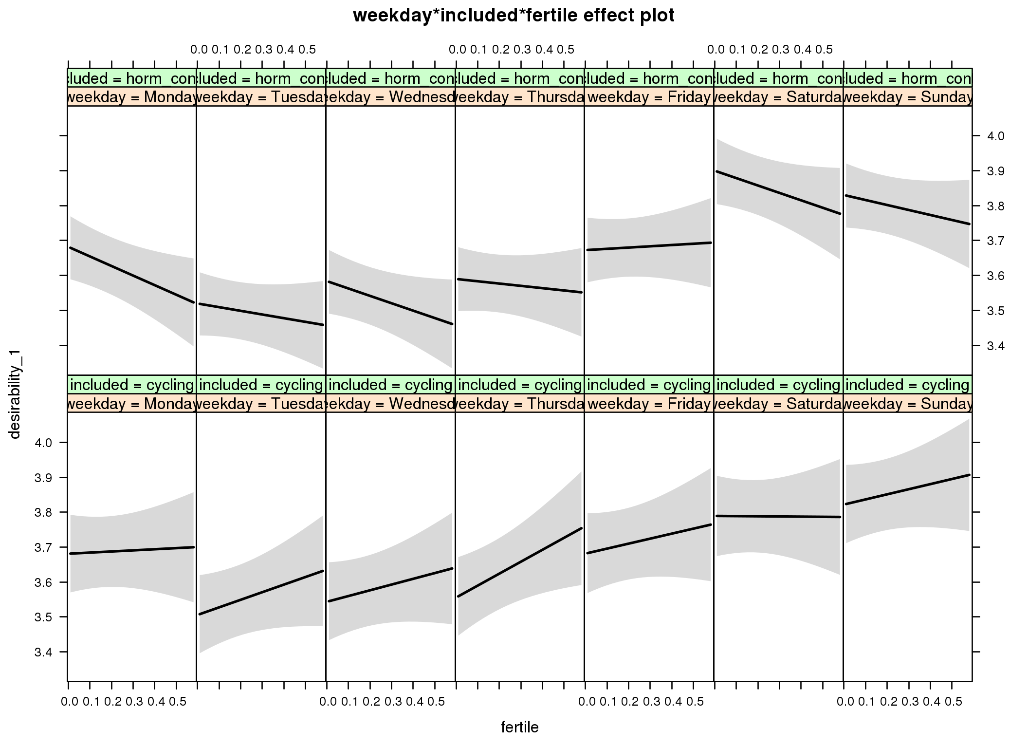
Linear mixed model fit by REML ['lmerMod']
Formula: desirability_1 ~ menstruation + fertile_mean + (1 | person) +
weekday + included + fertile + menstruation:included + weekday:included +
weekday:fertile + included:fertile + weekday:included:fertile
Data: diary
REML criterion at convergence: 84460
Scaled residuals:
Min 1Q Median 3Q Max
-4.110 -0.623 0.035 0.663 3.571
Random effects:
Groups Name Variance Std.Dev.
person (Intercept) 0.728 0.853
Residual 1.251 1.118
Number of obs: 26685, groups: person, 1054
Fixed effects:
Estimate Std. Error t value
(Intercept) 3.742494 0.083280 44.9
menstruationpre -0.110728 0.034124 -3.2
menstruationyes -0.254110 0.032146 -7.9
fertile_mean 0.015023 0.348003 0.0
weekdayTuesday -0.175309 0.053233 -3.3
weekdayWednesday -0.137642 0.053143 -2.6
weekdayThursday -0.125515 0.053749 -2.3
weekdayFriday 0.000305 0.054657 0.0
weekdaySaturday 0.108288 0.055201 2.0
weekdaySunday 0.140945 0.053347 2.6
includedhorm_contra -0.017268 0.076178 -0.2
fertile 0.032089 0.149918 0.2
menstruationpre:includedhorm_contra 0.026300 0.043806 0.6
menstruationyes:includedhorm_contra 0.076766 0.042145 1.8
weekdayTuesday:includedhorm_contra 0.013002 0.068385 0.2
weekdayWednesday:includedhorm_contra 0.039471 0.068610 0.6
weekdayThursday:includedhorm_contra 0.033453 0.069263 0.5
weekdayFriday:includedhorm_contra -0.009712 0.070213 -0.1
weekdaySaturday:includedhorm_contra 0.109794 0.071032 1.5
weekdaySunday:includedhorm_contra 0.007429 0.068856 0.1
weekdayTuesday:fertile 0.185243 0.206371 0.9
weekdayWednesday:fertile 0.132472 0.207340 0.6
weekdayThursday:fertile 0.310233 0.210303 1.5
weekdayFriday:fertile 0.110999 0.210677 0.5
weekdaySaturday:fertile -0.037271 0.213479 -0.2
weekdaySunday:fertile 0.114142 0.207460 0.6
includedhorm_contra:fertile -0.306496 0.191748 -1.6
weekdayTuesday:includedhorm_contra:fertile -0.016108 0.263402 -0.1
weekdayWednesday:includedhorm_contra:fertile -0.069843 0.265478 -0.3
weekdayThursday:includedhorm_contra:fertile -0.101779 0.267608 -0.4
weekdayFriday:includedhorm_contra:fertile 0.199966 0.268454 0.7
weekdaySaturday:includedhorm_contra:fertile 0.099463 0.272330 0.4
weekdaySunday:includedhorm_contra:fertile 0.017305 0.265005 0.1
M_m5: Moderation by exclusion threshold
model %>%
test_moderator("included_levels", diary, xlevels = 4)refitting model(s) with ML (instead of REML)
| Df | AIC | BIC | logLik | deviance | Chisq | Chi Df | Pr(>Chisq) | |
|---|---|---|---|---|---|---|---|---|
| with_main | 17 | 84654 | 84793 | -42310 | 84620 | NA | NA | NA |
| with_mod | 23 | 84660 | 84849 | -42307 | 84614 | 5.418 | 6 | 0.4914 |

Linear mixed model fit by REML ['lmerMod']
Formula: desirability_1 ~ menstruation + fertile_mean + (1 | person) +
included_levels + included + fertile + menstruation:included +
included_levels:included + included_levels:fertile + included:fertile +
included_levels:included:fertile
Data: diary
REML criterion at convergence: 84680
Scaled residuals:
Min 1Q Median 3Q Max
-4.048 -0.629 0.028 0.659 3.664
Random effects:
Groups Name Variance Std.Dev.
person (Intercept) 0.726 0.852
Residual 1.264 1.124
Number of obs: 26685, groups: person, 1054
Fixed effects:
Estimate Std. Error t value
(Intercept) 3.63081 0.08408 43.2
menstruationpre -0.11299 0.03433 -3.3
menstruationyes -0.25344 0.03232 -7.8
fertile_mean -0.00629 0.35150 0.0
included_levelslax 0.18547 0.17081 1.1
included_levelsconservative 0.28056 0.13334 2.1
included_levelsstrict 0.21165 0.13118 1.6
includedhorm_contra 0.06094 0.08680 0.7
fertile 0.15781 0.08747 1.8
menstruationpre:includedhorm_contra 0.02706 0.04408 0.6
menstruationyes:includedhorm_contra 0.06870 0.04241 1.6
included_levelslax:includedhorm_contra -0.20062 0.20806 -1.0
included_levelsconservative:includedhorm_contra -0.25285 0.16671 -1.5
included_levelsstrict:includedhorm_contra -0.12881 0.16139 -0.8
included_levelslax:fertile 0.18515 0.21370 0.9
included_levelsconservative:fertile -0.13198 0.15958 -0.8
included_levelsstrict:fertile -0.01882 0.15969 -0.1
includedhorm_contra:fertile -0.15120 0.13348 -1.1
included_levelslax:includedhorm_contra:fertile -0.31641 0.26068 -1.2
included_levelsconservative:includedhorm_contra:fertile -0.11706 0.20743 -0.6
included_levelsstrict:includedhorm_contra:fertile -0.15414 0.20423 -0.8
M_m6: Moderation by cycle length
model %>%
test_moderator("cycle_length_groups", diary, xlevels = 4)refitting model(s) with ML (instead of REML)
| Df | AIC | BIC | logLik | deviance | Chisq | Chi Df | Pr(>Chisq) | |
|---|---|---|---|---|---|---|---|---|
| with_main | 17 | 84649 | 84788 | -42307 | 84615 | NA | NA | NA |
| with_mod | 23 | 84639 | 84827 | -42296 | 84593 | 21.99 | 6 | 0.001216 |
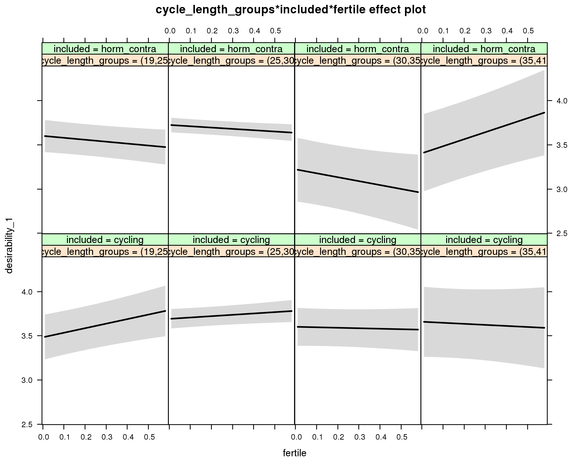
Linear mixed model fit by REML ['lmerMod']
Formula: desirability_1 ~ menstruation + fertile_mean + (1 | person) +
cycle_length_groups + included + fertile + menstruation:included +
cycle_length_groups:included + cycle_length_groups:fertile +
included:fertile + cycle_length_groups:included:fertile
Data: diary
REML criterion at convergence: 84651
Scaled residuals:
Min 1Q Median 3Q Max
-4.073 -0.624 0.030 0.662 3.630
Random effects:
Groups Name Variance Std.Dev.
person (Intercept) 0.723 0.85
Residual 1.263 1.12
Number of obs: 26685, groups: person, 1054
Fixed effects:
Estimate Std. Error t value
(Intercept) 3.5643 0.1439 24.77
menstruationpre -0.1125 0.0343 -3.28
menstruationyes -0.2604 0.0325 -8.00
fertile_mean -0.0893 0.3519 -0.25
cycle_length_groups(25,30] 0.2083 0.1412 1.48
cycle_length_groups(30,35] 0.1186 0.1697 0.70
cycle_length_groups(35,41] 0.1758 0.2404 0.73
includedhorm_contra 0.0985 0.1605 0.61
fertile 0.5136 0.1826 2.81
menstruationpre:includedhorm_contra 0.0283 0.0441 0.64
menstruationyes:includedhorm_contra 0.0793 0.0426 1.86
cycle_length_groups(25,30]:includedhorm_contra -0.0845 0.1741 -0.49
cycle_length_groups(30,35]:includedhorm_contra -0.4972 0.2669 -1.86
cycle_length_groups(35,41]:includedhorm_contra -0.3722 0.3407 -1.09
cycle_length_groups(25,30]:fertile -0.3614 0.1959 -1.85
cycle_length_groups(30,35]:fertile -0.5683 0.2319 -2.45
cycle_length_groups(35,41]:fertile -0.6321 0.3276 -1.93
includedhorm_contra:fertile -0.7319 0.2155 -3.40
cycle_length_groups(25,30]:includedhorm_contra:fertile 0.4307 0.2321 1.86
cycle_length_groups(30,35]:includedhorm_contra:fertile 0.3432 0.3652 0.94
cycle_length_groups(35,41]:includedhorm_contra:fertile 1.6425 0.4314 3.81
M_m7: Moderation by certainty about menstruation parameters
model %>%
test_moderator("certainty_menstruation", diary)refitting model(s) with ML (instead of REML)
| Df | AIC | BIC | logLik | deviance | Chisq | Chi Df | Pr(>Chisq) | |
|---|---|---|---|---|---|---|---|---|
| with_main | 13 | 84641 | 84747 | -42307 | 84615 | NA | NA | NA |
| with_mod | 15 | 84640 | 84763 | -42305 | 84610 | 4.2 | 2 | 0.1225 |
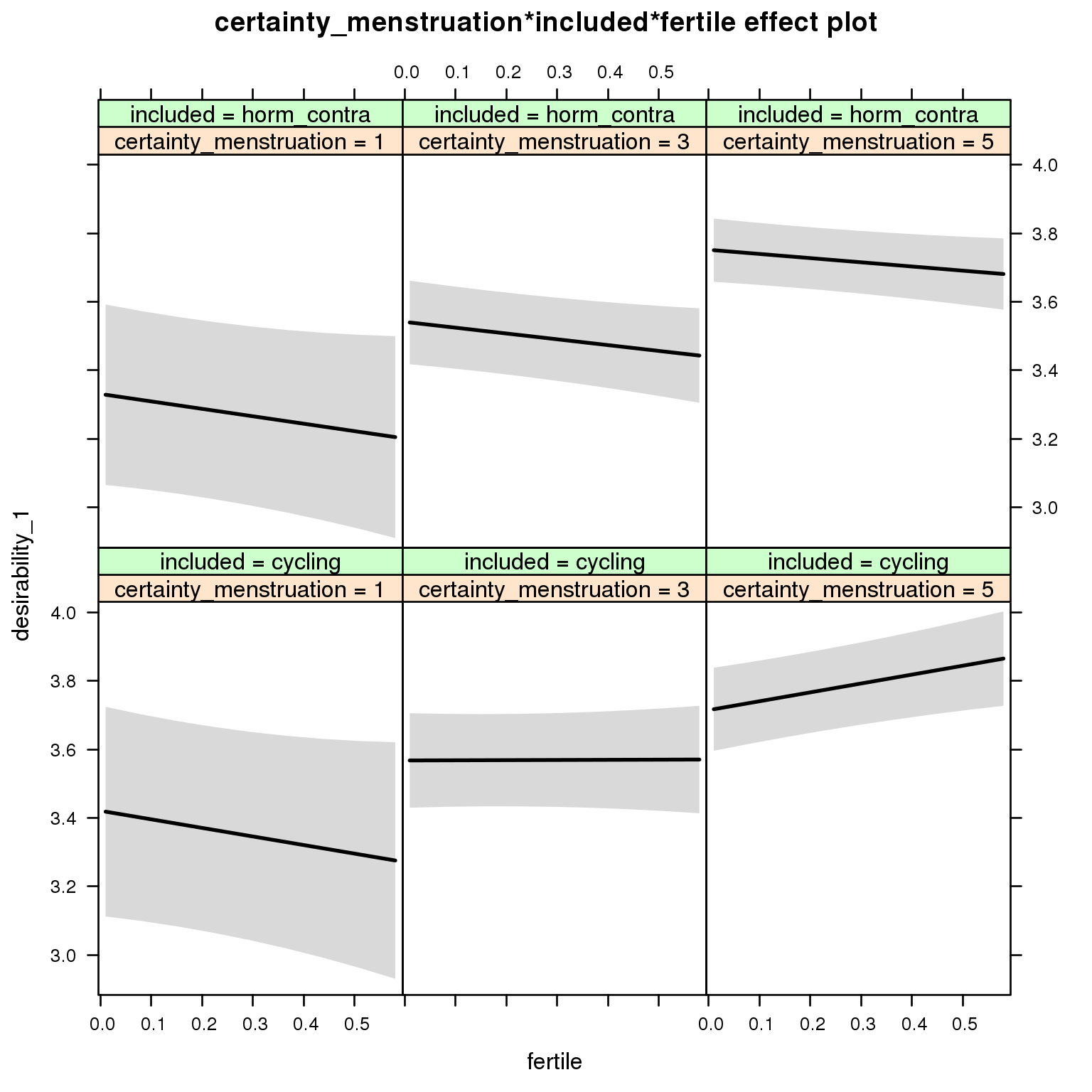
Linear mixed model fit by REML ['lmerMod']
Formula: desirability_1 ~ menstruation + fertile_mean + (1 | person) +
certainty_menstruation + included + fertile + menstruation:included +
certainty_menstruation:included + certainty_menstruation:fertile +
included:fertile + certainty_menstruation:included:fertile
Data: diary
REML criterion at convergence: 84666
Scaled residuals:
Min 1Q Median 3Q Max
-4.046 -0.629 0.031 0.661 3.661
Random effects:
Groups Name Variance Std.Dev.
person (Intercept) 0.719 0.848
Residual 1.264 1.124
Number of obs: 26685, groups: person, 1054
Fixed effects:
Estimate Std. Error t value
(Intercept) 3.4178 0.2105 16.24
menstruationpre -0.1087 0.0343 -3.17
menstruationyes -0.2486 0.0324 -7.69
fertile_mean -0.0466 0.3476 -0.13
certainty_menstruation 0.0735 0.0480 1.53
includedhorm_contra -0.1382 0.2672 -0.52
fertile -0.3775 0.2724 -1.39
menstruationpre:includedhorm_contra 0.0260 0.0440 0.59
menstruationyes:includedhorm_contra 0.0680 0.0424 1.60
certainty_menstruation:includedhorm_contra 0.0318 0.0622 0.51
certainty_menstruation:fertile 0.1274 0.0638 2.00
includedhorm_contra:fertile 0.1367 0.3540 0.39
certainty_menstruation:includedhorm_contra:fertile -0.1036 0.0818 -1.27
M_m8: Moderation by cycle regularity
model %>%
test_moderator("cycle_regularity", diary)refitting model(s) with ML (instead of REML)
| Df | AIC | BIC | logLik | deviance | Chisq | Chi Df | Pr(>Chisq) | |
|---|---|---|---|---|---|---|---|---|
| with_main | 15 | 84647 | 84770 | -42309 | 84617 | NA | NA | NA |
| with_mod | 19 | 84650 | 84806 | -42306 | 84612 | 5.382 | 4 | 0.2503 |
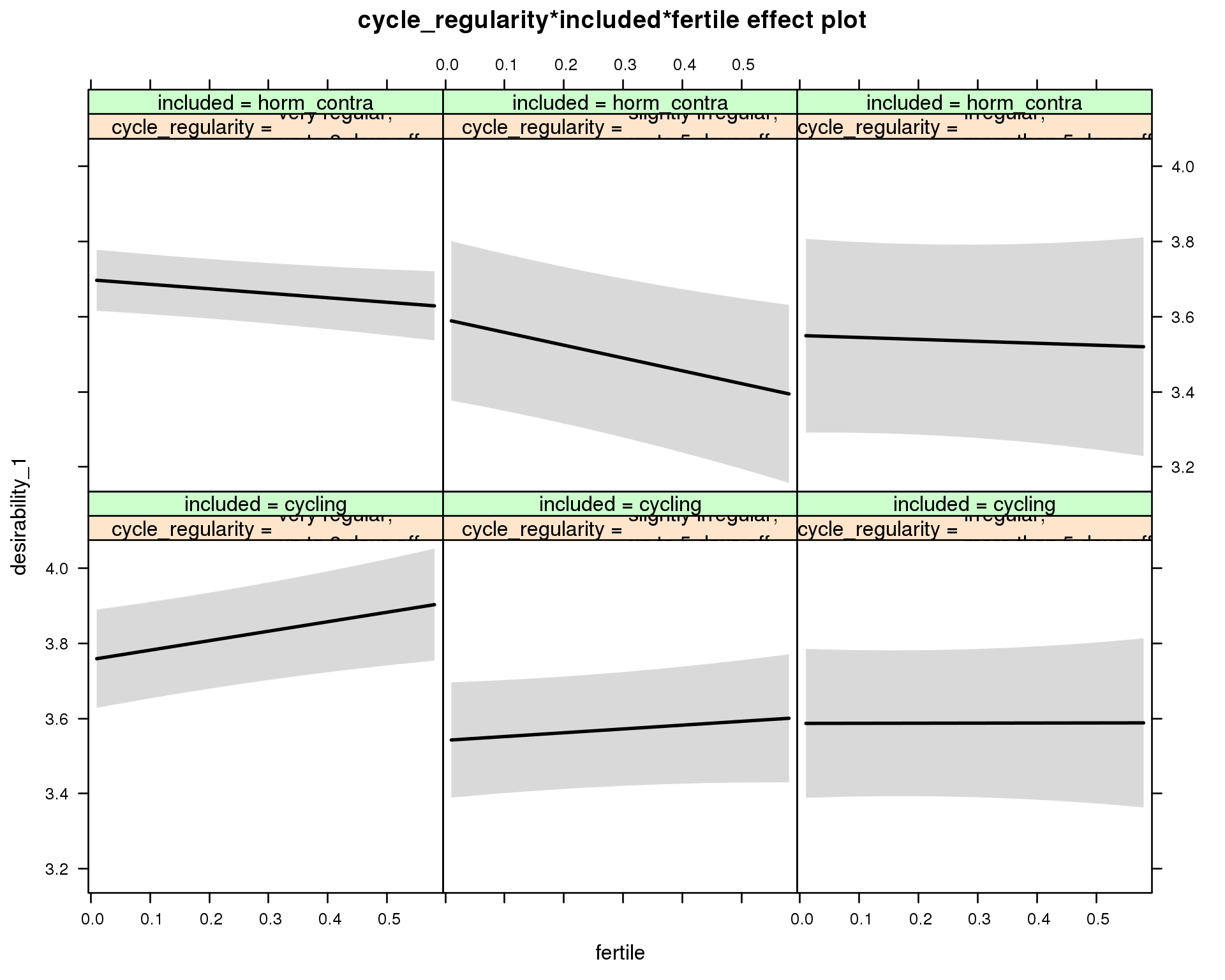
Linear mixed model fit by REML ['lmerMod']
Formula: desirability_1 ~ menstruation + fertile_mean + (1 | person) +
cycle_regularity + included + fertile + menstruation:included +
cycle_regularity:included + cycle_regularity:fertile + included:fertile +
cycle_regularity:included:fertile
Data: diary
REML criterion at convergence: 84668
Scaled residuals:
Min 1Q Median 3Q Max
-4.048 -0.627 0.030 0.658 3.679
Random effects:
Groups Name Variance Std.Dev.
person (Intercept) 0.723 0.851
Residual 1.264 1.124
Number of obs: 26685, groups: person, 1054
Fixed effects:
Estimate Std. Error t value
(Intercept) 3.8160 0.0892 42.8
menstruationpre -0.1094 0.0343 -3.2
menstruationyes -0.2508 0.0323 -7.8
fertile_mean 0.0205 0.3493 0.1
cycle_regularityslightly irregular,\nup to 5 days off -0.2148 0.1028 -2.1
cycle_regularityirregular,\nmore than 5 days off -0.1697 0.1211 -1.4
includedhorm_contra -0.0749 0.0810 -0.9
fertile 0.2523 0.0958 2.6
menstruationpre:includedhorm_contra 0.0256 0.0440 0.6
menstruationyes:includedhorm_contra 0.0691 0.0424 1.6
cycle_regularityslightly irregular,\nup to 5 days off:includedhorm_contra 0.1090 0.1552 0.7
cycle_regularityirregular,\nmore than 5 days off:includedhorm_contra 0.0215 0.1836 0.1
cycle_regularityslightly irregular,\nup to 5 days off:fertile -0.1510 0.1322 -1.1
cycle_regularityirregular,\nmore than 5 days off:fertile -0.2499 0.1625 -1.5
includedhorm_contra:fertile -0.3717 0.1123 -3.3
cycle_regularityslightly irregular,\nup to 5 days off:includedhorm_contra:fertile -0.0706 0.1963 -0.4
cycle_regularityirregular,\nmore than 5 days off:includedhorm_contra:fertile 0.3178 0.2424 1.3
M_m9: Moderation by cohabitation status
model %>%
test_moderator("cohabitation", diary)refitting model(s) with ML (instead of REML)
| Df | AIC | BIC | logLik | deviance | Chisq | Chi Df | Pr(>Chisq) | |
|---|---|---|---|---|---|---|---|---|
| with_main | 15 | 84646 | 84768 | -42308 | 84616 | NA | NA | NA |
| with_mod | 19 | 84641 | 84796 | -42301 | 84603 | 13.09 | 4 | 0.01086 |
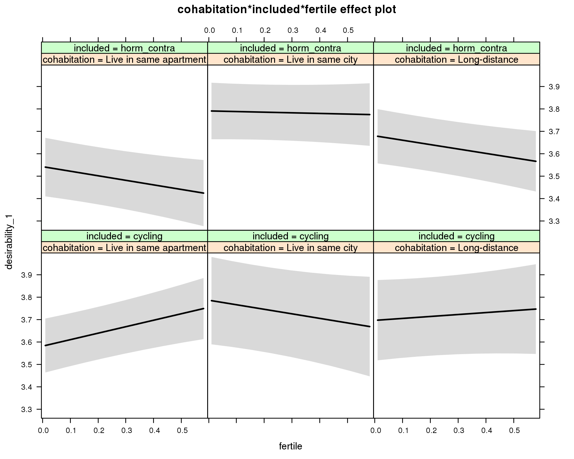
Linear mixed model fit by REML ['lmerMod']
Formula: desirability_1 ~ menstruation + fertile_mean + (1 | person) +
cohabitation + included + fertile + menstruation:included +
cohabitation:included + cohabitation:fertile + included:fertile + cohabitation:included:fertile
Data: diary
REML criterion at convergence: 84662
Scaled residuals:
Min 1Q Median 3Q Max
-4.037 -0.629 0.032 0.659 3.651
Random effects:
Groups Name Variance Std.Dev.
person (Intercept) 0.722 0.85
Residual 1.263 1.12
Number of obs: 26685, groups: person, 1054
Fixed effects:
Estimate Std. Error t value
(Intercept) 3.64548 0.08638 42.2
menstruationpre -0.11171 0.03429 -3.3
menstruationyes -0.25322 0.03231 -7.8
fertile_mean -0.00197 0.34828 0.0
cohabitationLive in same city 0.20479 0.11671 1.8
cohabitationLong-distance 0.11495 0.10999 1.0
includedhorm_contra -0.05580 0.09256 -0.6
fertile 0.28891 0.08651 3.3
menstruationpre:includedhorm_contra 0.02735 0.04402 0.6
menstruationyes:includedhorm_contra 0.07100 0.04235 1.7
cohabitationLive in same city:includedhorm_contra 0.04360 0.14910 0.3
cohabitationLong-distance:includedhorm_contra 0.02242 0.14266 0.2
cohabitationLive in same city:fertile -0.49148 0.15801 -3.1
cohabitationLong-distance:fertile -0.20217 0.14232 -1.4
includedhorm_contra:fertile -0.49206 0.12636 -3.9
cohabitationLive in same city:includedhorm_contra:fertile 0.66664 0.19757 3.4
cohabitationLong-distance:includedhorm_contra:fertile 0.20960 0.18334 1.1
M_m10: Moderation by relationship status
model %>%
test_moderator("relationship_status_clean", diary)refitting model(s) with ML (instead of REML)
| Df | AIC | BIC | logLik | deviance | Chisq | Chi Df | Pr(>Chisq) | |
|---|---|---|---|---|---|---|---|---|
| with_main | 15 | 84643 | 84766 | -42307 | 84613 | NA | NA | NA |
| with_mod | 19 | 84648 | 84803 | -42305 | 84610 | 3.789 | 4 | 0.4353 |
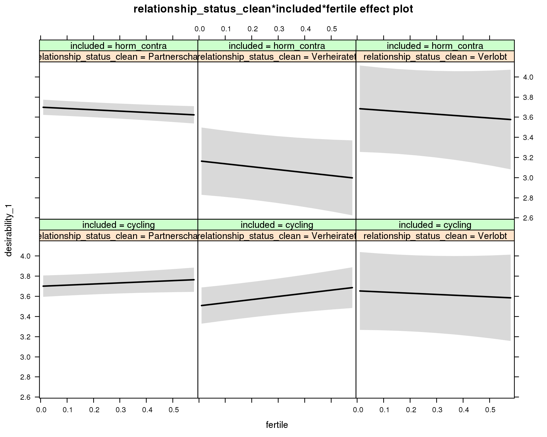
Linear mixed model fit by REML ['lmerMod']
Formula: desirability_1 ~ menstruation + fertile_mean + (1 | person) +
relationship_status_clean + included + fertile + menstruation:included +
relationship_status_clean:included + relationship_status_clean:fertile +
included:fertile + relationship_status_clean:included:fertile
Data: diary
REML criterion at convergence: 84660
Scaled residuals:
Min 1Q Median 3Q Max
-4.058 -0.626 0.032 0.660 3.659
Random effects:
Groups Name Variance Std.Dev.
person (Intercept) 0.719 0.848
Residual 1.264 1.124
Number of obs: 26685, groups: person, 1054
Fixed effects:
Estimate Std. Error t value
(Intercept) 3.76245 0.08068 46.6
menstruationpre -0.11160 0.03429 -3.3
menstruationyes -0.25226 0.03231 -7.8
fertile_mean 0.00803 0.34733 0.0
relationship_status_cleanVerheiratet -0.19461 0.10640 -1.8
relationship_status_cleanVerlobt -0.04559 0.20485 -0.2
includedhorm_contra -0.01763 0.06913 -0.3
fertile 0.11159 0.07924 1.4
menstruationpre:includedhorm_contra 0.02790 0.04403 0.6
menstruationyes:includedhorm_contra 0.07030 0.04235 1.7
relationship_status_cleanVerheiratet:includedhorm_contra -0.33862 0.20502 -1.7
relationship_status_cleanVerlobt:includedhorm_contra 0.03193 0.30268 0.1
relationship_status_cleanVerheiratet:fertile 0.20041 0.13951 1.4
relationship_status_cleanVerlobt:fertile -0.23067 0.26160 -0.9
includedhorm_contra:fertile -0.24289 0.09657 -2.5
relationship_status_cleanVerheiratet:includedhorm_contra:fertile -0.35969 0.26270 -1.4
relationship_status_cleanVerlobt:includedhorm_contra:fertile 0.17382 0.40633 0.4
Specific robustness checks for desirability
Although desirability is associated with self esteem, sexy and showy clothes, adjusting for them only makes the effect stronger.
summary(lmer(desirability_1 ~ self_esteem_1 + sexy_clothes + showy_clothes + included * (menstruation + fertile) + fertile_mean + ( 1 | person), data = diary))## Linear mixed model fit by REML
## t-tests use Satterthwaite approximations to degrees of freedom ['lmerMod']
## Formula: desirability_1 ~ self_esteem_1 + sexy_clothes + showy_clothes +
## included * (menstruation + fertile) + fertile_mean + (1 | person)
## Data: diary
##
## REML criterion at convergence: 75623
##
## Scaled residuals:
## Min 1Q Median 3Q Max
## -4.830 -0.591 0.001 0.604 5.555
##
## Random effects:
## Groups Name Variance Std.Dev.
## person (Intercept) 0.302 0.549
## Residual 0.917 0.957
## Number of obs: 26685, groups: person, 1054
##
## Fixed effects:
## Estimate Std. Error df t value Pr(>|t|)
## (Intercept) 0.49198 0.06121 2664.00000 8.04 1.3e-15 ***
## self_esteem_1 0.50159 0.00659 25770.00000 76.17 < 2e-16 ***
## sexy_clothes 0.32361 0.00727 26472.00000 44.52 < 2e-16 ***
## showy_clothes 0.03036 0.00610 26469.00000 4.97 6.6e-07 ***
## includedhorm_contra -0.00288 0.04320 1646.00000 -0.07 0.94694
## menstruationpre -0.05064 0.02914 26188.00000 -1.74 0.08226 .
## menstruationyes -0.14140 0.02745 26324.00000 -5.15 2.6e-07 ***
## fertile 0.20009 0.05882 26142.00000 3.40 0.00067 ***
## fertile_mean -0.08187 0.24433 1683.00000 -0.34 0.73761
## includedhorm_contra:menstruationpre -0.01248 0.03741 26184.00000 -0.33 0.73875
## includedhorm_contra:menstruationyes -0.02114 0.03597 26289.00000 -0.59 0.55683
## includedhorm_contra:fertile -0.32331 0.07443 26305.00000 -4.34 1.4e-05 ***
## ---
## Signif. codes: 0 '***' 0.001 '**' 0.01 '*' 0.05 '.' 0.1 ' ' 1
##
## Correlation of Fixed Effects:
## (Intr) slf__1 sxy_cl shwy_c incld_ mnstrtnp mnstrtny fertil frtl_m
## self_estm_1 -0.406
## sexy_cloths -0.149 -0.143
## showy_clths -0.055 -0.043 -0.524
## inclddhrm_c -0.409 0.013 -0.018 0.003
## menstrutnpr -0.195 0.008 0.013 0.002 0.271
## menstrutnys -0.199 0.022 0.019 0.005 0.259 0.395
## fertile -0.182 0.008 -0.001 0.004 0.333 0.466 0.383
## fertile_men -0.663 0.010 -0.011 -0.007 -0.029 -0.007 -0.005 -0.084
## inclddhrm_cntr:mnstrtnp 0.158 -0.008 -0.002 -0.002 -0.339 -0.779 -0.308 -0.362 -0.006
## inclddhrm_cntr:mnstrtny 0.156 -0.020 -0.008 -0.002 -0.319 -0.301 -0.763 -0.292 -0.006
## inclddhrm_cntr:f 0.181 -0.015 0.008 0.002 -0.421 -0.368 -0.302 -0.786 0.011
## inclddhrm_cntr:mnstrtnp inclddhrm_cntr:mnstrtny
## self_estm_1
## sexy_cloths
## showy_clths
## inclddhrm_c
## menstrutnpr
## menstrutnys
## fertile
## fertile_men
## inclddhrm_cntr:mnstrtnp
## inclddhrm_cntr:mnstrtny 0.380
## inclddhrm_cntr:f 0.466 0.380Petting
model_summaries$had_pettingModel summary
Model summary
model %>%
print_summary()Generalized linear mixed model fit by maximum likelihood (Laplace Approximation) ['glmerMod']
Family: binomial ( probit )
Formula: had_petting ~ included * (menstruation + fertile) + fertile_mean + (1 | person)
Data: diary
AIC BIC logLik deviance df.resid
24084 24166 -12032 24064 26693
Scaled residuals:
Min 1Q Median 3Q Max
-2.280 -0.498 -0.348 -0.176 5.359
Random effects:
Groups Name Variance Std.Dev.
person (Intercept) 0.368 0.607
Number of obs: 26703, groups: person, 1054
Fixed effects:
Estimate Std. Error z value Pr(>|z|)
(Intercept) -1.08824 0.06977 -15.60 < 2e-16 ***
includedhorm_contra 0.19491 0.05696 3.42 0.00062 ***
menstruationpre -0.06177 0.04916 -1.26 0.20894
menstruationyes -0.12024 0.04660 -2.58 0.00987 **
fertile 0.13222 0.09733 1.36 0.17432
fertile_mean -0.07059 0.32305 -0.22 0.82704
includedhorm_contra:menstruationpre 0.00543 0.06165 0.09 0.92977
includedhorm_contra:menstruationyes -0.03463 0.05984 -0.58 0.56277
includedhorm_contra:fertile -0.26705 0.12115 -2.20 0.02751 *
---
Signif. codes: 0 '***' 0.001 '**' 0.01 '*' 0.05 '.' 0.1 ' ' 1
Correlation of Fixed Effects:
(Intr) incld_ mnstrtnp mnstrtny fertil frtl_m inclddhrm_cntr:mnstrtnp
inclddhrm_c -0.489
menstrutnpr -0.273 0.339
menstrutnys -0.255 0.318 0.376
fertile -0.264 0.423 0.459 0.374
fertile_men -0.758 -0.035 -0.005 -0.005 -0.103
inclddhrm_cntr:mnstrtnp 0.227 -0.417 -0.797 -0.299 -0.365 -0.008
inclddhrm_cntr:mnstrtny 0.207 -0.383 -0.292 -0.779 -0.291 -0.006 0.363
inclddhrm_cntr:f 0.262 -0.523 -0.368 -0.300 -0.797 0.018 0.460
inclddhrm_cntr:mnstrtny
inclddhrm_c
menstrutnpr
menstrutnys
fertile
fertile_men
inclddhrm_cntr:mnstrtnp
inclddhrm_cntr:mnstrtny
inclddhrm_cntr:f 0.370
convergence code: 0
Model failed to converge with max|grad| = 0.0145105 (tol = 0.001, component 1)
Effect size standardised by residual variance (\(\frac{b}{ SD_{residual} }\)): 0.13 [-0.06;0.32].
Marginal effect plots
model %>%
plot_all_effects()
Outcome distribution
model %>%
plot_outcome(diary) + xlab(outcome_label)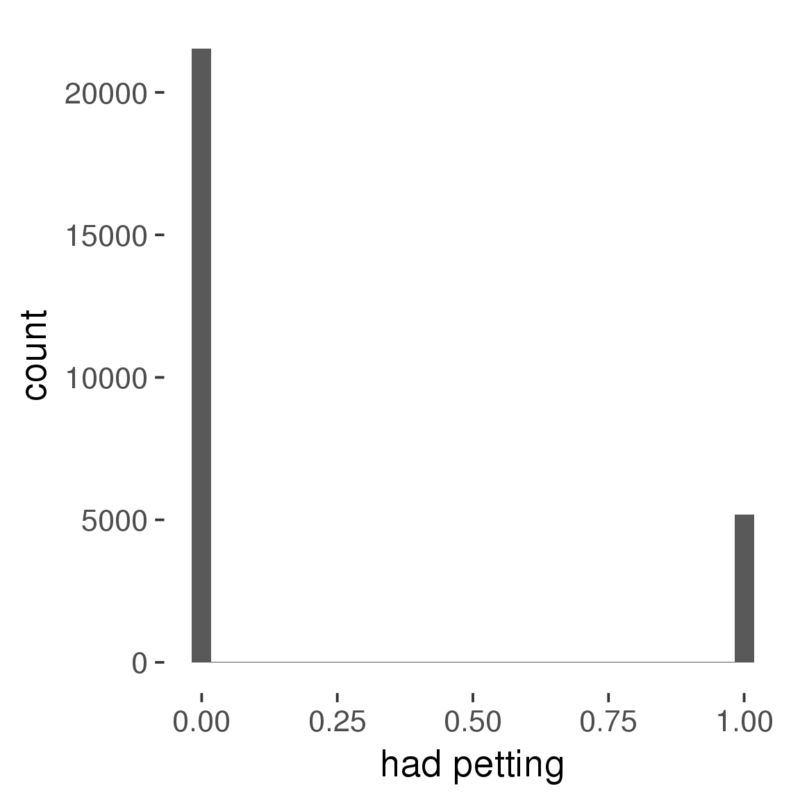
Diagnostics
model %>%
print_diagnostics()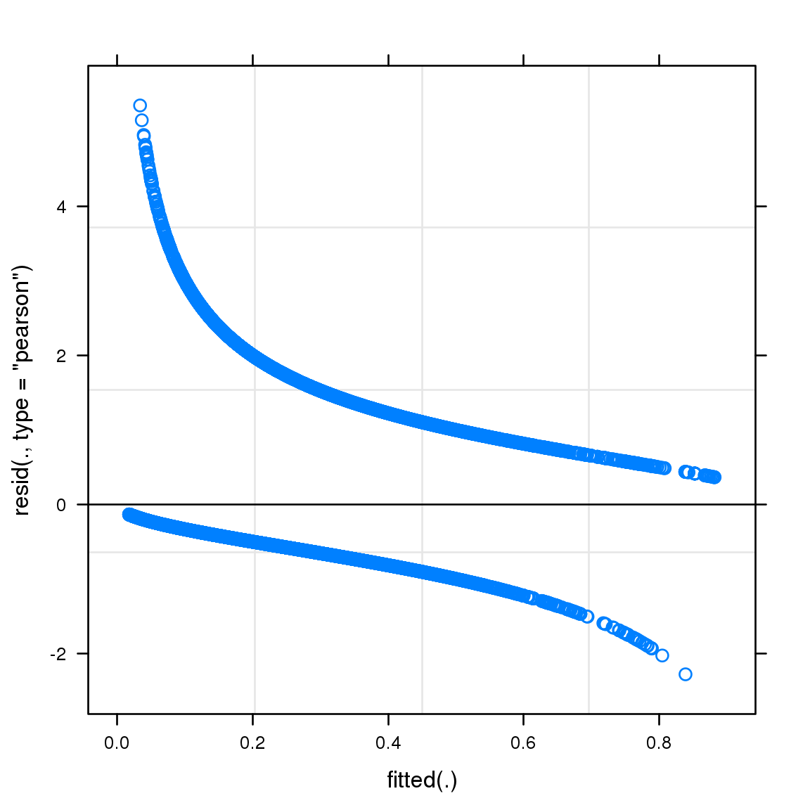
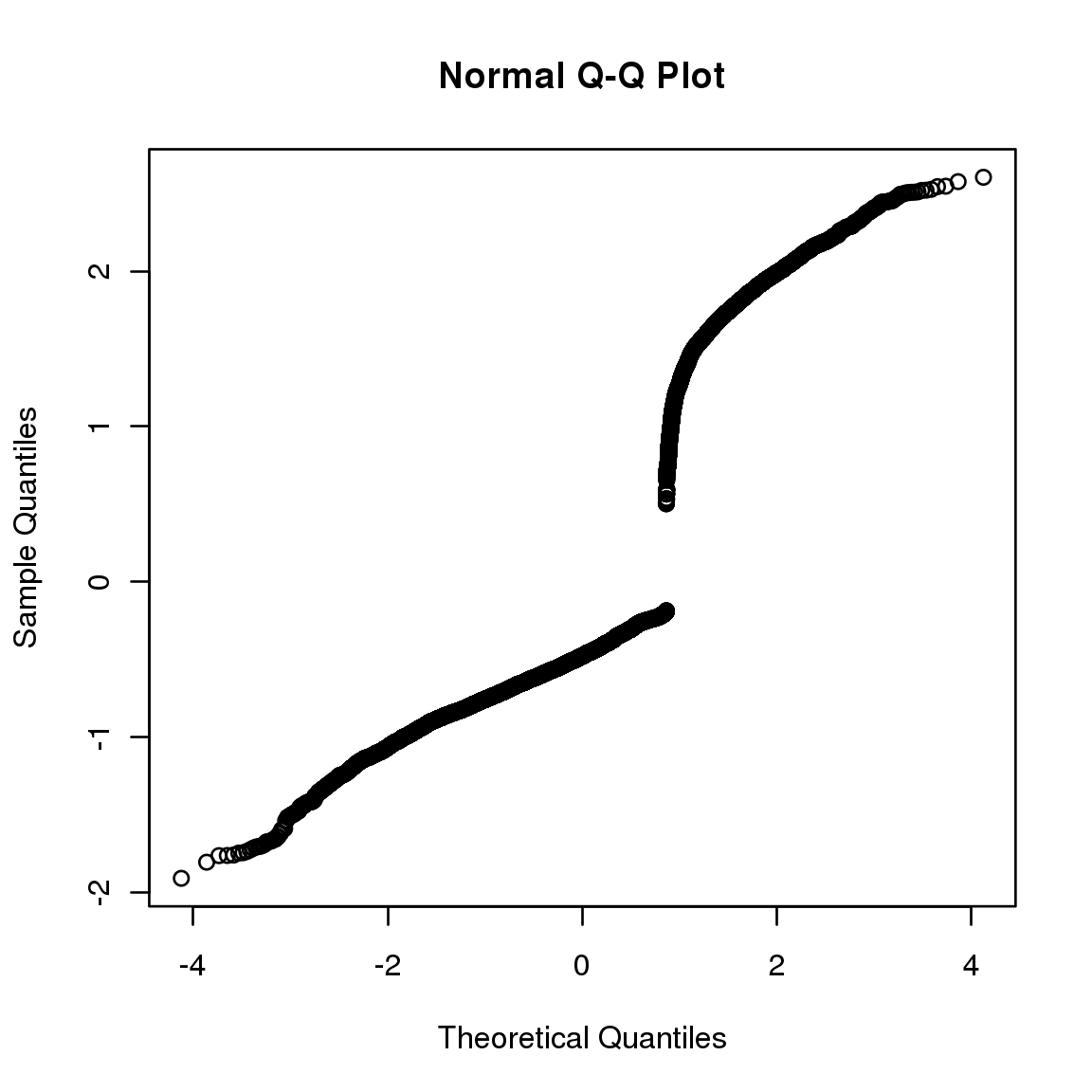

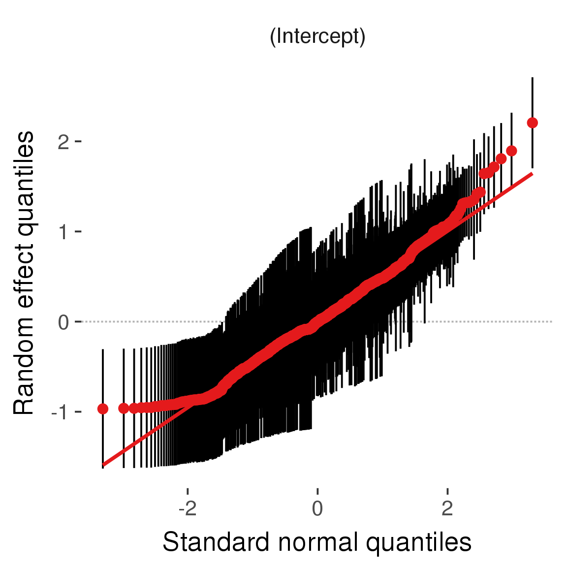
Curves
Here, we continuously plot the outcome over the course of the cycle. Because cycle lengths vary, we subset the data to cycles in a certain range. If the red curve traces the pink curve, our predictor accurately maps the relationship between fertile window probability and the outcome.
Cycle lengths from 21 to 36
Backward-counted
model %>%
plot_curve(diary %>% filter(minimum_cycle_length_diary <= 36, minimum_cycle_length_diary > 20) %>% mutate(fertile=prc_stirn_b))outcome = names(model@frame)[1]
outcome_label = recode(str_replace_all(str_replace_all(str_replace_all(outcome, "_", " "), " pair", "-pair"), " 1", ""),
"desirability 1" = "self-perceived desirability",
"NARQ admiration" = "narcissistic admiration",
"NARQ rivalry" = "narcissistic rivalry",
"extra-pair" = "extra-pair desire & behaviour",
"had sexual intercourse" = "sexual intercourse")
library(ggplot2)
# form a subset and run the model without the hormonal contraception and the fertility predictors
tmp = diary %>%
filter(!is.na(fertile), !is.na(included),
RCD > -1 * minimum_cycle_length_diary, RCD > -40)
new_form = update.formula(formula(model), new = . ~ . - fertile * included)
tmp$residuals = residuals(update(model, new_form, data = tmp , na.action = na.exclude))
tmp = tmp %>%
filter(!is.na(RCD), !is.na(residuals))
rcd_min = min(tmp$RCD)
tmp$real = FALSE
tmp_before = tmp
tmp_before$RCD = tmp_before$RCD + min(tmp$RCD) - 1
tmp_after = tmp
tmp_after$RCD = tmp_after$RCD - min(tmp$RCD) + 1
tmp$real = TRUE
tmp = bind_rows(tmp_before %>% filter(RCD > rcd_min - 11), tmp, tmp_after %>% filter(RCD < 11))GAM smooth on residuals
Here, we partialled out menstruation and individual random effects, then superimposed estimated probability of being in the fertile window scaled to the range of the estimated means. To address the periodicity of the cycle, we prepended and appended ten days of the timeseries to the end and the beginning of the timeseries. We then estimated the GAM and cut off the appended subsets before plotting.
tryCatch({
trend_plot = ggplot(tmp,aes(x = RCD, y = residuals, colour = included)) +
stat_smooth(geom = 'smooth',size = 0.8, fill = "#9ECAE1", method = 'gam', formula = y ~ s(x))
}, error = function(e){cat_message(e, "danger")})
tryCatch({
trend_data = ggplot_build(trend_plot)$data[[1]]
}, error = function(e){cat_message(e, "danger")})
trend_data$RCD = round(trend_data$x)
trend_data = left_join(trend_data, tmp %>% select(real, RCD,fertile) %>% unique(), by = "RCD")
trend_data %>%
filter(real == TRUE) %>%
mutate(superimposed = ( ( (fertile - 0.01)/0.58) * (max(y)-min(y) ) ) + min(y) ) ->
trend_data
ggplot(trend_data) +
geom_ribbon(aes(x = x, ymin = ymin, ymax = ymax, fill = factor(group)), alpha = 0.2) +
geom_line(aes(x = x, y = y, colour = factor(group)), size = 0.8, stat = "identity") +
scale_x_continuous(caption_x) +
geom_line(aes(x = x, y = superimposed), color = "#a83fbf", size = 1, linetype = 'dashed') +
annotate("text",x = mean(trend_data$x), y = max(trend_data$superimposed,na.rm=T) + 0.1, label = 'superimposed fertility peak', color = "#a83fbf") +
scale_y_continuous(outcome_label) +
ggtitle("GAM smooth, residuals") +
scale_color_manual("Contraception status",values = c("2"="black","1"= "red"), labels = c("2"="hormonally\ncontracepting","1"="cycling"), guide = F) +
scale_fill_manual("Contraception status",values = c("2"="black","1"= "red"), labels = c("2"="hormonally\ncontracepting","1"="cycling"), guide = F)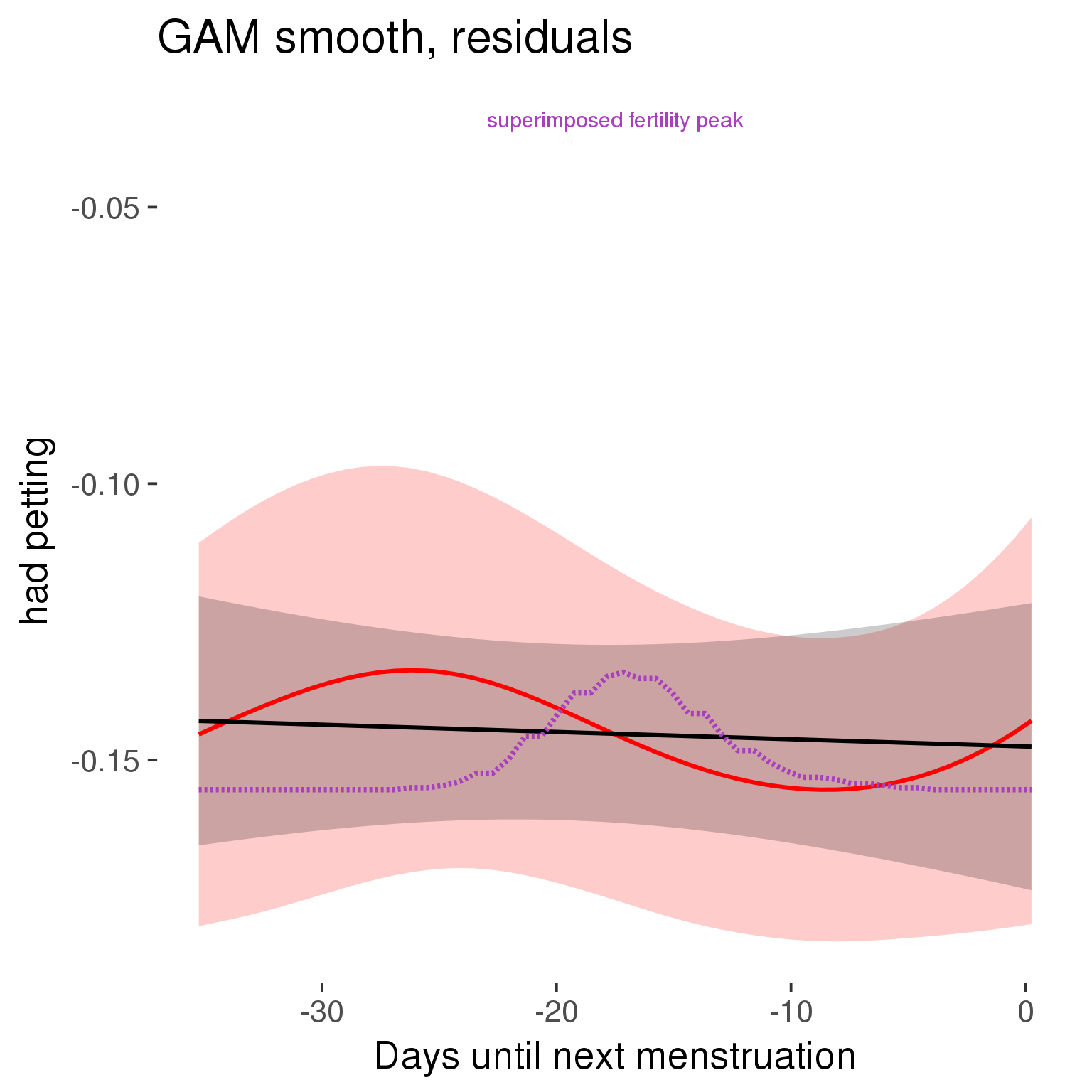
GAM smooth on raw data
As before, but without partialling anything out.
tryCatch({
trend_plot = ggplot(tmp,aes_string(x = "RCD", y = outcome, colour = "included")) +
stat_smooth(geom = 'smooth',size = 0.8, fill = "#9ECAE1", method = 'gam', formula = y ~ s(x))
}, error = function(e){cat_message(e, "danger")})
tryCatch({
trend_data = ggplot_build(trend_plot)$data[[1]]
}, error = function(e){cat_message(e, "danger")})
trend_data$RCD = round(trend_data$x)
trend_data = left_join(trend_data, tmp %>% select(real, RCD,fertile) %>% unique(), by = "RCD")
trend_data %>%
filter(real == TRUE) %>%
mutate(superimposed = ( ( (fertile - 0.01)/0.58) * (max(y)-min(y) ) ) + min(y) ) ->
trend_data
plot1b = ggplot(trend_data) +
geom_ribbon(aes(x = x, ymin = ymin, ymax = ymax, fill = factor(group)), alpha = 0.2) +
geom_line(aes(x = x, y = y, colour = factor(group)), size = 0.8, stat = "identity") +
scale_x_continuous(caption_x) +
geom_line(aes(x = x, y = superimposed), color = "#a83fbf", size = 1, linetype = 'dashed') +
annotate("text",x = mean(trend_data$x), y = max(trend_data$superimposed,na.rm=T) + 0.1, label = 'superimposed fertility peak', color = "#a83fbf") +
scale_y_continuous(outcome_label) +
ggtitle("GAM smooth, raw data") +
scale_color_manual("Contraception status",values = c("2"="black","1"= "red"), labels = c("2"="hormonally\ncontracepting","1"="cycling"), guide = F) +
scale_fill_manual("Contraception status",values = c("2"="black","1"= "red"), labels = c("2"="hormonally\ncontracepting","1"="cycling"), guide = F)
suppressWarnings(print(plot1b))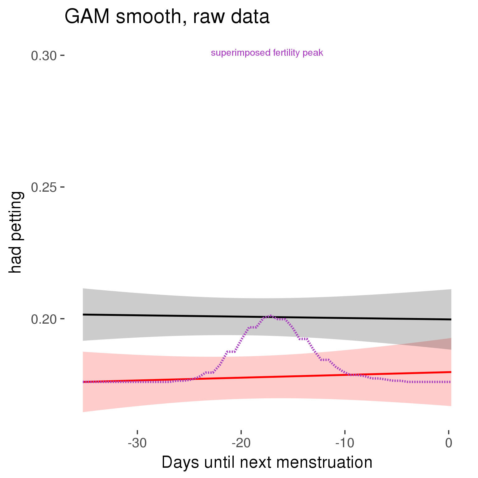
Means and standard errors over raw data
Nothing partialled out, just straight means with bootstrapped confidence intervals.
tryCatch({
trend_plot = ggplot(tmp,aes_string(x = "RCD", y = outcome, colour = "included")) +
geom_pointrange(size = 0.8, stat = 'summary', fun.data = "mean_cl_boot")
}, error = function(e){cat_message(e, "danger")})
tryCatch({
trend_data = ggplot_build(trend_plot)$data[[1]]
}, error = function(e){cat_message(e, "danger")})
trend_data$RCD = round(trend_data$x)
trend_data = left_join(trend_data, tmp %>% select(real, RCD,fertile) %>% unique(), by = "RCD")
trend_data %>%
filter(real == TRUE) %>%
mutate(superimposed = ( ( (fertile - 0.01)/0.58) * (max(y)-min(y) ) ) + min(y) ) ->
trend_data
plot3 = ggplot(trend_data) +
geom_pointrange(aes(x = x, y = y, ymin = ymin,ymax = ymax, colour = factor(group)), size = 0.8, stat = "identity", alpha = 0.6, position = position_dodge(width = .5)) +
scale_x_continuous("Days until next menstruation") +
geom_line(aes(x= x, y = superimposed), color = "#a83fbf", size = 1, linetype = 'dashed') +
annotate("text",x = mean(trend_data$x), y = max(trend_data$superimposed,na.rm=T) + 0.1, label = 'superimposed fertility peak', color = "#a83fbf") +
scale_y_continuous(outcome_label) +
ggtitle("Means with standard errors, raw data") +
scale_color_manual("Contraception status",values = c("2"="black","1"= "red"), labels = c("2"="hormonally\ncontracepting","1"="cycling"), guide = F) +
scale_fill_manual("Contraception status",values = c("2"="black","1"= "red"), labels = c("2"="hormonally\ncontracepting","1"="cycling"), guide = F)
suppressWarnings(print(plot3))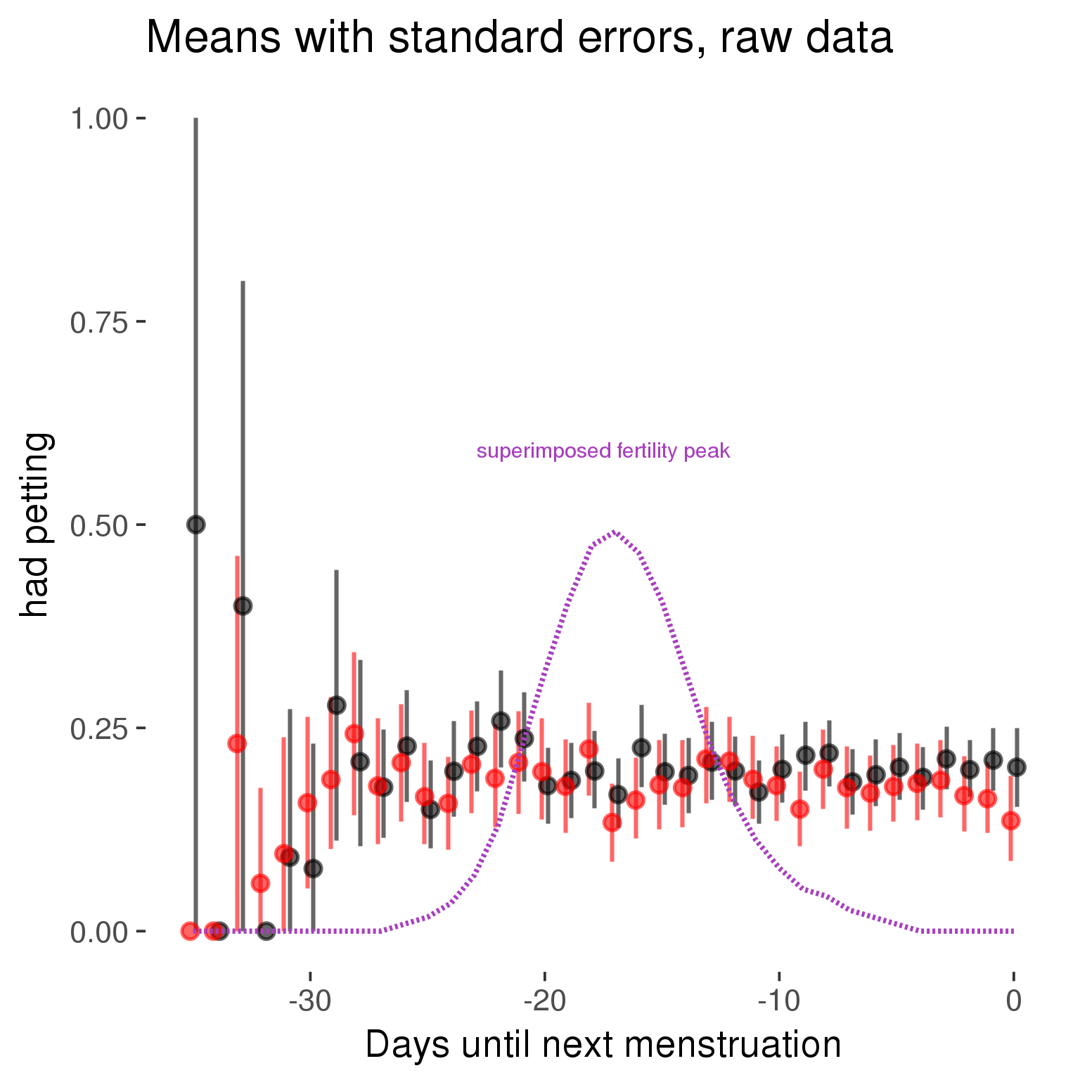
Forward-counted
model %>%
plot_curve(diary %>% filter(minimum_cycle_length_diary <= 36, minimum_cycle_length_diary > 20) %>% mutate(RCD = FCD, fertile = prc_stirn_b_forward_counted), caption_x = "Days since last menstruation")outcome = names(model@frame)[1]
outcome_label = recode(str_replace_all(str_replace_all(str_replace_all(outcome, "_", " "), " pair", "-pair"), " 1", ""),
"desirability 1" = "self-perceived desirability",
"NARQ admiration" = "narcissistic admiration",
"NARQ rivalry" = "narcissistic rivalry",
"extra-pair" = "extra-pair desire & behaviour",
"had sexual intercourse" = "sexual intercourse")
library(ggplot2)
# form a subset and run the model without the hormonal contraception and the fertility predictors
tmp = diary %>%
filter(!is.na(fertile), !is.na(included),
RCD > -1 * minimum_cycle_length_diary, RCD > -40)
new_form = update.formula(formula(model), new = . ~ . - fertile * included)
tmp$residuals = residuals(update(model, new_form, data = tmp , na.action = na.exclude))
tmp = tmp %>%
filter(!is.na(RCD), !is.na(residuals))
rcd_min = min(tmp$RCD)
tmp$real = FALSE
tmp_before = tmp
tmp_before$RCD = tmp_before$RCD + min(tmp$RCD) - 1
tmp_after = tmp
tmp_after$RCD = tmp_after$RCD - min(tmp$RCD) + 1
tmp$real = TRUE
tmp = bind_rows(tmp_before %>% filter(RCD > rcd_min - 11), tmp, tmp_after %>% filter(RCD < 11))GAM smooth on residuals
Here, we partialled out menstruation and individual random effects, then superimposed estimated probability of being in the fertile window scaled to the range of the estimated means. To address the periodicity of the cycle, we prepended and appended ten days of the timeseries to the end and the beginning of the timeseries. We then estimated the GAM and cut off the appended subsets before plotting.
tryCatch({
trend_plot = ggplot(tmp,aes(x = RCD, y = residuals, colour = included)) +
stat_smooth(geom = 'smooth',size = 0.8, fill = "#9ECAE1", method = 'gam', formula = y ~ s(x))
}, error = function(e){cat_message(e, "danger")})
tryCatch({
trend_data = ggplot_build(trend_plot)$data[[1]]
}, error = function(e){cat_message(e, "danger")})
trend_data$RCD = round(trend_data$x)
trend_data = left_join(trend_data, tmp %>% select(real, RCD,fertile) %>% unique(), by = "RCD")
trend_data %>%
filter(real == TRUE) %>%
mutate(superimposed = ( ( (fertile - 0.01)/0.58) * (max(y)-min(y) ) ) + min(y) ) ->
trend_data
ggplot(trend_data) +
geom_ribbon(aes(x = x, ymin = ymin, ymax = ymax, fill = factor(group)), alpha = 0.2) +
geom_line(aes(x = x, y = y, colour = factor(group)), size = 0.8, stat = "identity") +
scale_x_continuous(caption_x) +
geom_line(aes(x = x, y = superimposed), color = "#a83fbf", size = 1, linetype = 'dashed') +
annotate("text",x = mean(trend_data$x), y = max(trend_data$superimposed,na.rm=T) + 0.1, label = 'superimposed fertility peak', color = "#a83fbf") +
scale_y_continuous(outcome_label) +
ggtitle("GAM smooth, residuals") +
scale_color_manual("Contraception status",values = c("2"="black","1"= "red"), labels = c("2"="hormonally\ncontracepting","1"="cycling"), guide = F) +
scale_fill_manual("Contraception status",values = c("2"="black","1"= "red"), labels = c("2"="hormonally\ncontracepting","1"="cycling"), guide = F)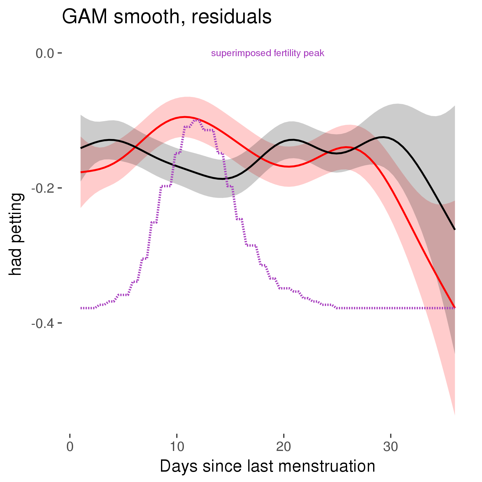
GAM smooth on raw data
As before, but without partialling anything out.
tryCatch({
trend_plot = ggplot(tmp,aes_string(x = "RCD", y = outcome, colour = "included")) +
stat_smooth(geom = 'smooth',size = 0.8, fill = "#9ECAE1", method = 'gam', formula = y ~ s(x))
}, error = function(e){cat_message(e, "danger")})
tryCatch({
trend_data = ggplot_build(trend_plot)$data[[1]]
}, error = function(e){cat_message(e, "danger")})
trend_data$RCD = round(trend_data$x)
trend_data = left_join(trend_data, tmp %>% select(real, RCD,fertile) %>% unique(), by = "RCD")
trend_data %>%
filter(real == TRUE) %>%
mutate(superimposed = ( ( (fertile - 0.01)/0.58) * (max(y)-min(y) ) ) + min(y) ) ->
trend_data
plot1b = ggplot(trend_data) +
geom_ribbon(aes(x = x, ymin = ymin, ymax = ymax, fill = factor(group)), alpha = 0.2) +
geom_line(aes(x = x, y = y, colour = factor(group)), size = 0.8, stat = "identity") +
scale_x_continuous(caption_x) +
geom_line(aes(x = x, y = superimposed), color = "#a83fbf", size = 1, linetype = 'dashed') +
annotate("text",x = mean(trend_data$x), y = max(trend_data$superimposed,na.rm=T) + 0.1, label = 'superimposed fertility peak', color = "#a83fbf") +
scale_y_continuous(outcome_label) +
ggtitle("GAM smooth, raw data") +
scale_color_manual("Contraception status",values = c("2"="black","1"= "red"), labels = c("2"="hormonally\ncontracepting","1"="cycling"), guide = F) +
scale_fill_manual("Contraception status",values = c("2"="black","1"= "red"), labels = c("2"="hormonally\ncontracepting","1"="cycling"), guide = F)
suppressWarnings(print(plot1b))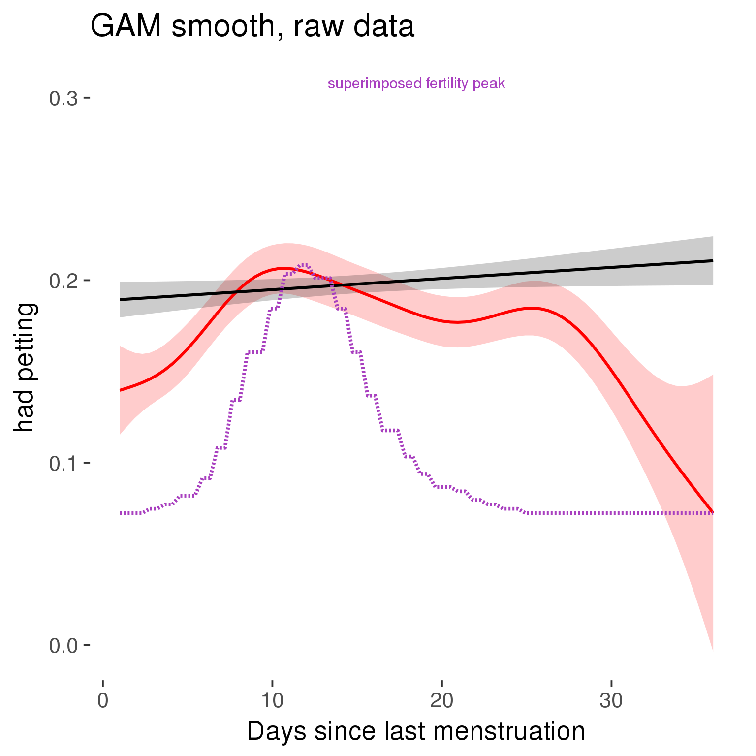
Means and standard errors over raw data
Nothing partialled out, just straight means with bootstrapped confidence intervals.
tryCatch({
trend_plot = ggplot(tmp,aes_string(x = "RCD", y = outcome, colour = "included")) +
geom_pointrange(size = 0.8, stat = 'summary', fun.data = "mean_cl_boot")
}, error = function(e){cat_message(e, "danger")})
tryCatch({
trend_data = ggplot_build(trend_plot)$data[[1]]
}, error = function(e){cat_message(e, "danger")})
trend_data$RCD = round(trend_data$x)
trend_data = left_join(trend_data, tmp %>% select(real, RCD,fertile) %>% unique(), by = "RCD")
trend_data %>%
filter(real == TRUE) %>%
mutate(superimposed = ( ( (fertile - 0.01)/0.58) * (max(y)-min(y) ) ) + min(y) ) ->
trend_data
plot3 = ggplot(trend_data) +
geom_pointrange(aes(x = x, y = y, ymin = ymin,ymax = ymax, colour = factor(group)), size = 0.8, stat = "identity", alpha = 0.6, position = position_dodge(width = .5)) +
scale_x_continuous("Days until next menstruation") +
geom_line(aes(x= x, y = superimposed), color = "#a83fbf", size = 1, linetype = 'dashed') +
annotate("text",x = mean(trend_data$x), y = max(trend_data$superimposed,na.rm=T) + 0.1, label = 'superimposed fertility peak', color = "#a83fbf") +
scale_y_continuous(outcome_label) +
ggtitle("Means with standard errors, raw data") +
scale_color_manual("Contraception status",values = c("2"="black","1"= "red"), labels = c("2"="hormonally\ncontracepting","1"="cycling"), guide = F) +
scale_fill_manual("Contraception status",values = c("2"="black","1"= "red"), labels = c("2"="hormonally\ncontracepting","1"="cycling"), guide = F)
suppressWarnings(print(plot3))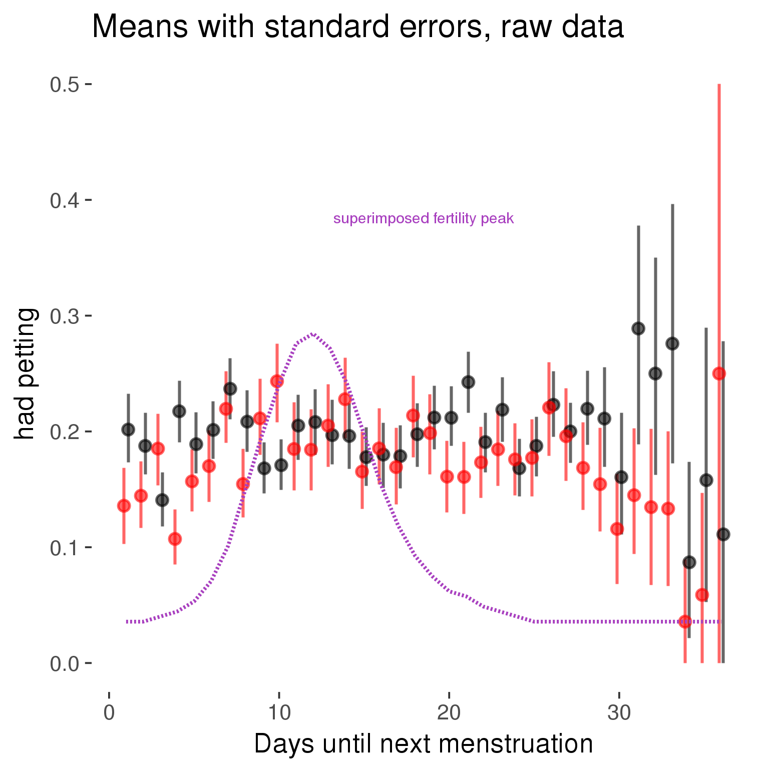
Cycle lengths from 27 to 30
Backward-counted
model %>%
plot_curve(diary %>% filter(minimum_cycle_length_diary <= 30, minimum_cycle_length_diary >= 27) %>% mutate(fertile=prc_stirn_b))outcome = names(model@frame)[1]
outcome_label = recode(str_replace_all(str_replace_all(str_replace_all(outcome, "_", " "), " pair", "-pair"), " 1", ""),
"desirability 1" = "self-perceived desirability",
"NARQ admiration" = "narcissistic admiration",
"NARQ rivalry" = "narcissistic rivalry",
"extra-pair" = "extra-pair desire & behaviour",
"had sexual intercourse" = "sexual intercourse")
library(ggplot2)
# form a subset and run the model without the hormonal contraception and the fertility predictors
tmp = diary %>%
filter(!is.na(fertile), !is.na(included),
RCD > -1 * minimum_cycle_length_diary, RCD > -40)
new_form = update.formula(formula(model), new = . ~ . - fertile * included)
tmp$residuals = residuals(update(model, new_form, data = tmp , na.action = na.exclude))
tmp = tmp %>%
filter(!is.na(RCD), !is.na(residuals))
rcd_min = min(tmp$RCD)
tmp$real = FALSE
tmp_before = tmp
tmp_before$RCD = tmp_before$RCD + min(tmp$RCD) - 1
tmp_after = tmp
tmp_after$RCD = tmp_after$RCD - min(tmp$RCD) + 1
tmp$real = TRUE
tmp = bind_rows(tmp_before %>% filter(RCD > rcd_min - 11), tmp, tmp_after %>% filter(RCD < 11))GAM smooth on residuals
Here, we partialled out menstruation and individual random effects, then superimposed estimated probability of being in the fertile window scaled to the range of the estimated means. To address the periodicity of the cycle, we prepended and appended ten days of the timeseries to the end and the beginning of the timeseries. We then estimated the GAM and cut off the appended subsets before plotting.
tryCatch({
trend_plot = ggplot(tmp,aes(x = RCD, y = residuals, colour = included)) +
stat_smooth(geom = 'smooth',size = 0.8, fill = "#9ECAE1", method = 'gam', formula = y ~ s(x))
}, error = function(e){cat_message(e, "danger")})
tryCatch({
trend_data = ggplot_build(trend_plot)$data[[1]]
}, error = function(e){cat_message(e, "danger")})
trend_data$RCD = round(trend_data$x)
trend_data = left_join(trend_data, tmp %>% select(real, RCD,fertile) %>% unique(), by = "RCD")
trend_data %>%
filter(real == TRUE) %>%
mutate(superimposed = ( ( (fertile - 0.01)/0.58) * (max(y)-min(y) ) ) + min(y) ) ->
trend_data
ggplot(trend_data) +
geom_ribbon(aes(x = x, ymin = ymin, ymax = ymax, fill = factor(group)), alpha = 0.2) +
geom_line(aes(x = x, y = y, colour = factor(group)), size = 0.8, stat = "identity") +
scale_x_continuous(caption_x) +
geom_line(aes(x = x, y = superimposed), color = "#a83fbf", size = 1, linetype = 'dashed') +
annotate("text",x = mean(trend_data$x), y = max(trend_data$superimposed,na.rm=T) + 0.1, label = 'superimposed fertility peak', color = "#a83fbf") +
scale_y_continuous(outcome_label) +
ggtitle("GAM smooth, residuals") +
scale_color_manual("Contraception status",values = c("2"="black","1"= "red"), labels = c("2"="hormonally\ncontracepting","1"="cycling"), guide = F) +
scale_fill_manual("Contraception status",values = c("2"="black","1"= "red"), labels = c("2"="hormonally\ncontracepting","1"="cycling"), guide = F)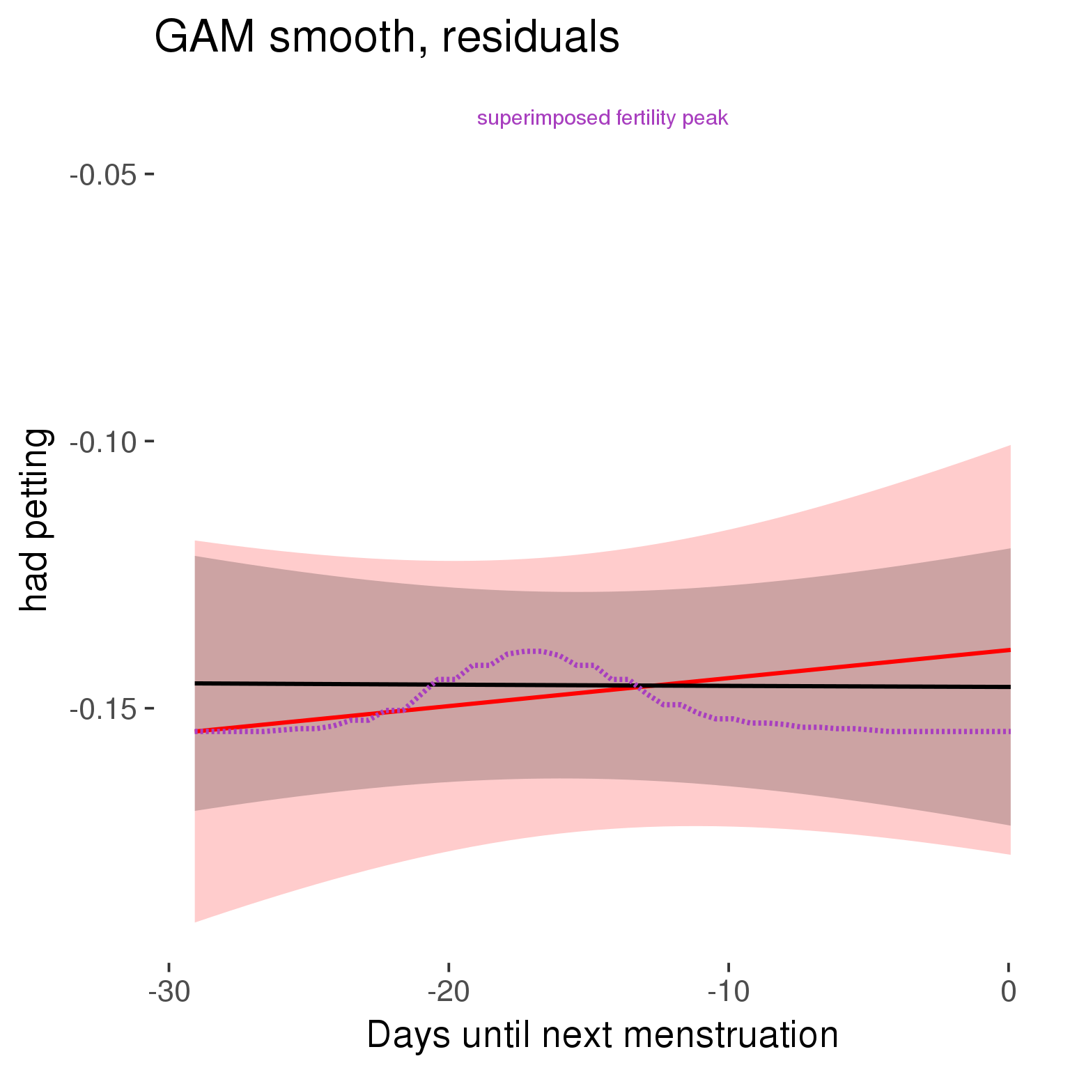
GAM smooth on raw data
As before, but without partialling anything out.
tryCatch({
trend_plot = ggplot(tmp,aes_string(x = "RCD", y = outcome, colour = "included")) +
stat_smooth(geom = 'smooth',size = 0.8, fill = "#9ECAE1", method = 'gam', formula = y ~ s(x))
}, error = function(e){cat_message(e, "danger")})
tryCatch({
trend_data = ggplot_build(trend_plot)$data[[1]]
}, error = function(e){cat_message(e, "danger")})
trend_data$RCD = round(trend_data$x)
trend_data = left_join(trend_data, tmp %>% select(real, RCD,fertile) %>% unique(), by = "RCD")
trend_data %>%
filter(real == TRUE) %>%
mutate(superimposed = ( ( (fertile - 0.01)/0.58) * (max(y)-min(y) ) ) + min(y) ) ->
trend_data
plot1b = ggplot(trend_data) +
geom_ribbon(aes(x = x, ymin = ymin, ymax = ymax, fill = factor(group)), alpha = 0.2) +
geom_line(aes(x = x, y = y, colour = factor(group)), size = 0.8, stat = "identity") +
scale_x_continuous(caption_x) +
geom_line(aes(x = x, y = superimposed), color = "#a83fbf", size = 1, linetype = 'dashed') +
annotate("text",x = mean(trend_data$x), y = max(trend_data$superimposed,na.rm=T) + 0.1, label = 'superimposed fertility peak', color = "#a83fbf") +
scale_y_continuous(outcome_label) +
ggtitle("GAM smooth, raw data") +
scale_color_manual("Contraception status",values = c("2"="black","1"= "red"), labels = c("2"="hormonally\ncontracepting","1"="cycling"), guide = F) +
scale_fill_manual("Contraception status",values = c("2"="black","1"= "red"), labels = c("2"="hormonally\ncontracepting","1"="cycling"), guide = F)
suppressWarnings(print(plot1b))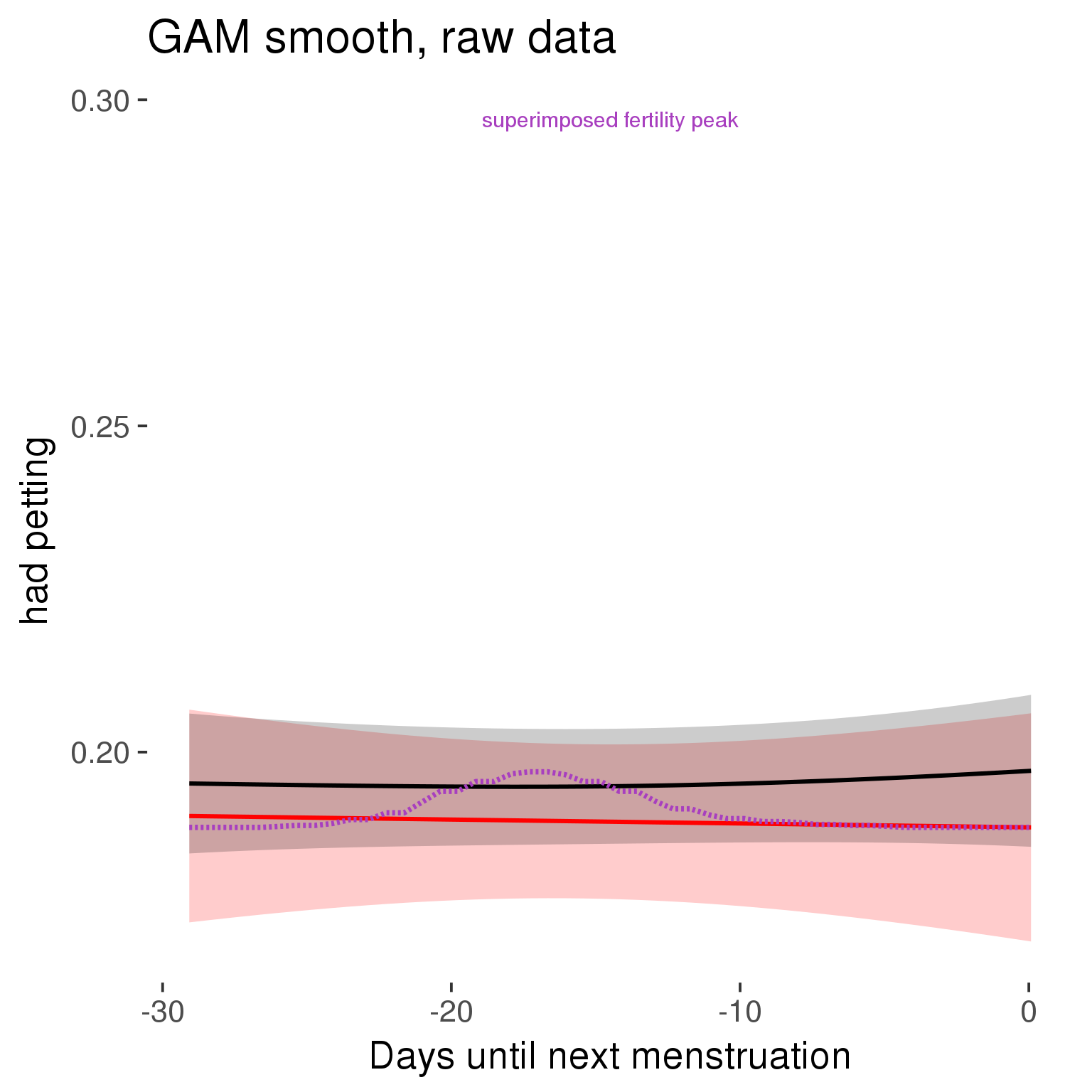
Means and standard errors over raw data
Nothing partialled out, just straight means with bootstrapped confidence intervals.
tryCatch({
trend_plot = ggplot(tmp,aes_string(x = "RCD", y = outcome, colour = "included")) +
geom_pointrange(size = 0.8, stat = 'summary', fun.data = "mean_cl_boot")
}, error = function(e){cat_message(e, "danger")})
tryCatch({
trend_data = ggplot_build(trend_plot)$data[[1]]
}, error = function(e){cat_message(e, "danger")})
trend_data$RCD = round(trend_data$x)
trend_data = left_join(trend_data, tmp %>% select(real, RCD,fertile) %>% unique(), by = "RCD")
trend_data %>%
filter(real == TRUE) %>%
mutate(superimposed = ( ( (fertile - 0.01)/0.58) * (max(y)-min(y) ) ) + min(y) ) ->
trend_data
plot3 = ggplot(trend_data) +
geom_pointrange(aes(x = x, y = y, ymin = ymin,ymax = ymax, colour = factor(group)), size = 0.8, stat = "identity", alpha = 0.6, position = position_dodge(width = .5)) +
scale_x_continuous("Days until next menstruation") +
geom_line(aes(x= x, y = superimposed), color = "#a83fbf", size = 1, linetype = 'dashed') +
annotate("text",x = mean(trend_data$x), y = max(trend_data$superimposed,na.rm=T) + 0.1, label = 'superimposed fertility peak', color = "#a83fbf") +
scale_y_continuous(outcome_label) +
ggtitle("Means with standard errors, raw data") +
scale_color_manual("Contraception status",values = c("2"="black","1"= "red"), labels = c("2"="hormonally\ncontracepting","1"="cycling"), guide = F) +
scale_fill_manual("Contraception status",values = c("2"="black","1"= "red"), labels = c("2"="hormonally\ncontracepting","1"="cycling"), guide = F)
suppressWarnings(print(plot3))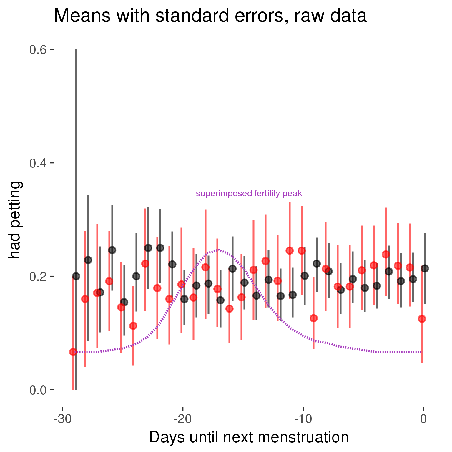
Forward-counted
model %>%
plot_curve(diary %>% filter(minimum_cycle_length_diary <= 30, minimum_cycle_length_diary >= 27) %>% mutate(RCD = FCD, fertile = prc_stirn_b_forward_counted), caption_x = "Days since last menstruation")outcome = names(model@frame)[1]
outcome_label = recode(str_replace_all(str_replace_all(str_replace_all(outcome, "_", " "), " pair", "-pair"), " 1", ""),
"desirability 1" = "self-perceived desirability",
"NARQ admiration" = "narcissistic admiration",
"NARQ rivalry" = "narcissistic rivalry",
"extra-pair" = "extra-pair desire & behaviour",
"had sexual intercourse" = "sexual intercourse")
library(ggplot2)
# form a subset and run the model without the hormonal contraception and the fertility predictors
tmp = diary %>%
filter(!is.na(fertile), !is.na(included),
RCD > -1 * minimum_cycle_length_diary, RCD > -40)
new_form = update.formula(formula(model), new = . ~ . - fertile * included)
tmp$residuals = residuals(update(model, new_form, data = tmp , na.action = na.exclude))
tmp = tmp %>%
filter(!is.na(RCD), !is.na(residuals))
rcd_min = min(tmp$RCD)
tmp$real = FALSE
tmp_before = tmp
tmp_before$RCD = tmp_before$RCD + min(tmp$RCD) - 1
tmp_after = tmp
tmp_after$RCD = tmp_after$RCD - min(tmp$RCD) + 1
tmp$real = TRUE
tmp = bind_rows(tmp_before %>% filter(RCD > rcd_min - 11), tmp, tmp_after %>% filter(RCD < 11))GAM smooth on residuals
Here, we partialled out menstruation and individual random effects, then superimposed estimated probability of being in the fertile window scaled to the range of the estimated means. To address the periodicity of the cycle, we prepended and appended ten days of the timeseries to the end and the beginning of the timeseries. We then estimated the GAM and cut off the appended subsets before plotting.
tryCatch({
trend_plot = ggplot(tmp,aes(x = RCD, y = residuals, colour = included)) +
stat_smooth(geom = 'smooth',size = 0.8, fill = "#9ECAE1", method = 'gam', formula = y ~ s(x))
}, error = function(e){cat_message(e, "danger")})
tryCatch({
trend_data = ggplot_build(trend_plot)$data[[1]]
}, error = function(e){cat_message(e, "danger")})
trend_data$RCD = round(trend_data$x)
trend_data = left_join(trend_data, tmp %>% select(real, RCD,fertile) %>% unique(), by = "RCD")
trend_data %>%
filter(real == TRUE) %>%
mutate(superimposed = ( ( (fertile - 0.01)/0.58) * (max(y)-min(y) ) ) + min(y) ) ->
trend_data
ggplot(trend_data) +
geom_ribbon(aes(x = x, ymin = ymin, ymax = ymax, fill = factor(group)), alpha = 0.2) +
geom_line(aes(x = x, y = y, colour = factor(group)), size = 0.8, stat = "identity") +
scale_x_continuous(caption_x) +
geom_line(aes(x = x, y = superimposed), color = "#a83fbf", size = 1, linetype = 'dashed') +
annotate("text",x = mean(trend_data$x), y = max(trend_data$superimposed,na.rm=T) + 0.1, label = 'superimposed fertility peak', color = "#a83fbf") +
scale_y_continuous(outcome_label) +
ggtitle("GAM smooth, residuals") +
scale_color_manual("Contraception status",values = c("2"="black","1"= "red"), labels = c("2"="hormonally\ncontracepting","1"="cycling"), guide = F) +
scale_fill_manual("Contraception status",values = c("2"="black","1"= "red"), labels = c("2"="hormonally\ncontracepting","1"="cycling"), guide = F)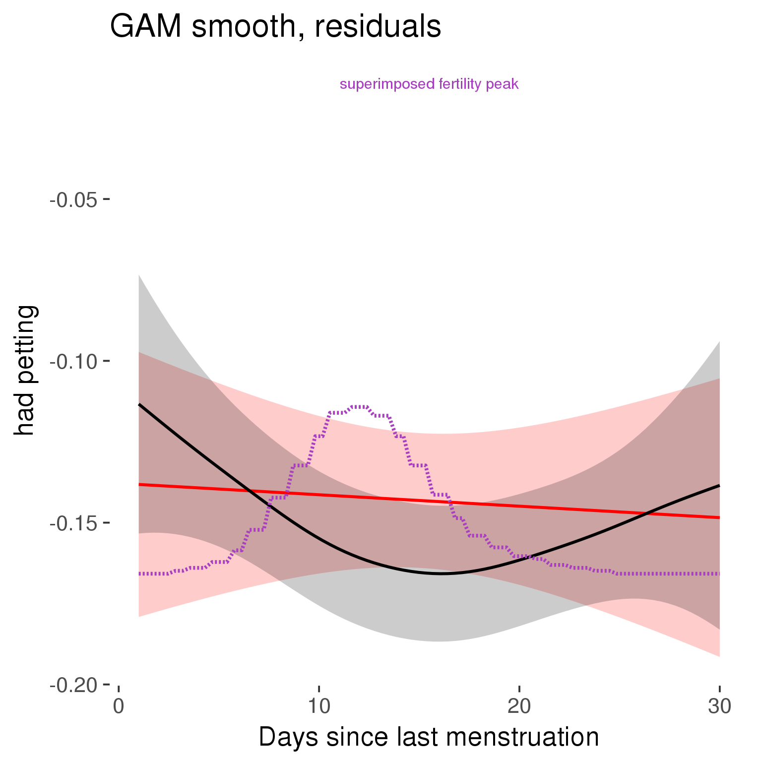
GAM smooth on raw data
As before, but without partialling anything out.
tryCatch({
trend_plot = ggplot(tmp,aes_string(x = "RCD", y = outcome, colour = "included")) +
stat_smooth(geom = 'smooth',size = 0.8, fill = "#9ECAE1", method = 'gam', formula = y ~ s(x))
}, error = function(e){cat_message(e, "danger")})
tryCatch({
trend_data = ggplot_build(trend_plot)$data[[1]]
}, error = function(e){cat_message(e, "danger")})
trend_data$RCD = round(trend_data$x)
trend_data = left_join(trend_data, tmp %>% select(real, RCD,fertile) %>% unique(), by = "RCD")
trend_data %>%
filter(real == TRUE) %>%
mutate(superimposed = ( ( (fertile - 0.01)/0.58) * (max(y)-min(y) ) ) + min(y) ) ->
trend_data
plot1b = ggplot(trend_data) +
geom_ribbon(aes(x = x, ymin = ymin, ymax = ymax, fill = factor(group)), alpha = 0.2) +
geom_line(aes(x = x, y = y, colour = factor(group)), size = 0.8, stat = "identity") +
scale_x_continuous(caption_x) +
geom_line(aes(x = x, y = superimposed), color = "#a83fbf", size = 1, linetype = 'dashed') +
annotate("text",x = mean(trend_data$x), y = max(trend_data$superimposed,na.rm=T) + 0.1, label = 'superimposed fertility peak', color = "#a83fbf") +
scale_y_continuous(outcome_label) +
ggtitle("GAM smooth, raw data") +
scale_color_manual("Contraception status",values = c("2"="black","1"= "red"), labels = c("2"="hormonally\ncontracepting","1"="cycling"), guide = F) +
scale_fill_manual("Contraception status",values = c("2"="black","1"= "red"), labels = c("2"="hormonally\ncontracepting","1"="cycling"), guide = F)
suppressWarnings(print(plot1b))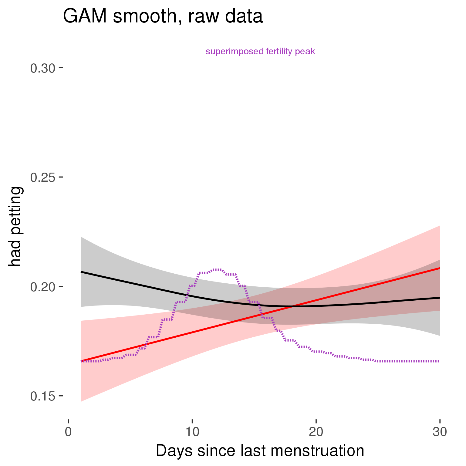
Means and standard errors over raw data
Nothing partialled out, just straight means with bootstrapped confidence intervals.
tryCatch({
trend_plot = ggplot(tmp,aes_string(x = "RCD", y = outcome, colour = "included")) +
geom_pointrange(size = 0.8, stat = 'summary', fun.data = "mean_cl_boot")
}, error = function(e){cat_message(e, "danger")})
tryCatch({
trend_data = ggplot_build(trend_plot)$data[[1]]
}, error = function(e){cat_message(e, "danger")})
trend_data$RCD = round(trend_data$x)
trend_data = left_join(trend_data, tmp %>% select(real, RCD,fertile) %>% unique(), by = "RCD")
trend_data %>%
filter(real == TRUE) %>%
mutate(superimposed = ( ( (fertile - 0.01)/0.58) * (max(y)-min(y) ) ) + min(y) ) ->
trend_data
plot3 = ggplot(trend_data) +
geom_pointrange(aes(x = x, y = y, ymin = ymin,ymax = ymax, colour = factor(group)), size = 0.8, stat = "identity", alpha = 0.6, position = position_dodge(width = .5)) +
scale_x_continuous("Days until next menstruation") +
geom_line(aes(x= x, y = superimposed), color = "#a83fbf", size = 1, linetype = 'dashed') +
annotate("text",x = mean(trend_data$x), y = max(trend_data$superimposed,na.rm=T) + 0.1, label = 'superimposed fertility peak', color = "#a83fbf") +
scale_y_continuous(outcome_label) +
ggtitle("Means with standard errors, raw data") +
scale_color_manual("Contraception status",values = c("2"="black","1"= "red"), labels = c("2"="hormonally\ncontracepting","1"="cycling"), guide = F) +
scale_fill_manual("Contraception status",values = c("2"="black","1"= "red"), labels = c("2"="hormonally\ncontracepting","1"="cycling"), guide = F)
suppressWarnings(print(plot3))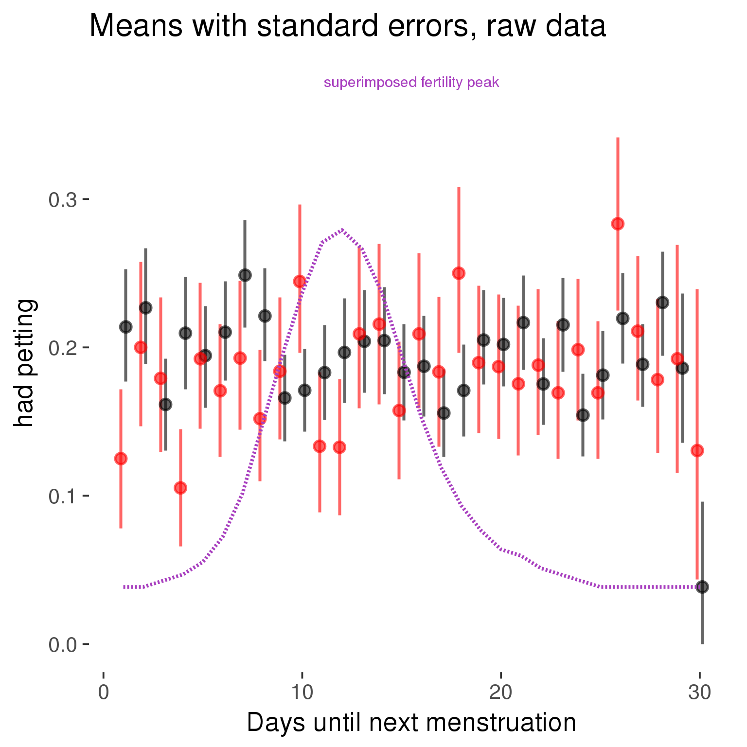
Robustness checks
M_r1: Random slopes for conception risk and menstruation
tryCatch({
# refit model with random effects for fertile and menstruation dummies
with_ind_diff = update(model, formula = . ~ . - (1| person) + (1 + fertile + menstruation | person))
# pull the random effects, format as tibble
rand = coef(with_ind_diff)$person %>%
tibble::rownames_to_column("person") %>%
mutate(person = as.numeric(person))
# pull the fixed effects
fixd = data.frame(fixef(with_ind_diff)) %>%
tibble::rownames_to_column("effect")
names(fixd) = c("effect", "pop_effect_size")
# pull apart the coefficients so that we can account for the fact that the random effect variation implicitly includes HC explaining the mean population-level effect of fertile/menstruation dummies among HC users
fixd = fixd %>%
separate(effect, c("included", "effect"), sep = ":", fill = "left") %>%
mutate(included = if_else(is.na(included), "cycling", str_replace(included, "included", "")))
fixd[2,c("included", "effect")] = c("horm_contra", "(Intercept)")
rand = rand %>%
# merge diary data on the random effects, so that we know who is a HC users and who isn't
inner_join(diary %>% select(person, included) %>% unique(), by = 'person') %>%
# gather into long format, to have the dataset by predictor
gather(effect, value, -person, -included) %>%
inner_join(fixd, by = c('effect', 'included')) %>%
# pull the fixed effects
mutate(
# only for those who are HC users, add the moderated population effect size for this effect (the random effects have the reference category mean)
value = if_else(included == "horm_contra", value + pop_effect_size, value),
effect = recode(effect, "includedhorm_contra" = "HC user",
"includedhorm_contra:fertile" = "HC user x fertile",
"includedhorm_contra:menstruationpre" = "HC user x premens.",
"includedhorm_contra:menstruationyes" = "HC user x mens.",
"menstruationyes" = "mens.",
"menstruationpre" = "premens.")) %>%
group_by(included, effect) %>%
# filter out predictors that aren't modelled as varying/random
filter(sd(value) > 0)
# plot dot plot of random effects
print(
ggplot(rand, aes(x = included, y = value, color = included, fill = included)) +
facet_wrap( ~ effect, scales = "free") +
# geom_violin(alpha = 0.4, size = 0) +
geom_dotplot(binaxis='y', dotsize = 0.1, method = "histodot") +
# geom_jitter(alpha = 0.05) +
coord_flip() +
geom_pointrange(stat = 'summary', fun.data = 'mean_sdl', color = 'darkred', size = 1.2) +
scale_color_manual("Contraception status", values = c("horm_contra"="black","cycling"= "red"), labels = c("horm_contra"="hormonally\ncontracepting","cycling"="cycling"), guide = F) +
scale_fill_manual("Contraception status", values = c("horm_contra"="black","cycling"= "red"), labels = c("horm_contra"="hormonally\ncontracepting","1"="cycling"), guide = F) +
ggtitle("M_r1: allowing participant-varying slopes", subtitle = "for the conception risk measure and the menstruation dummies") +
scale_x_discrete("Hormonal contraception", breaks = c("horm_contra", "cycling"), labels = c("yes", "no")) +
scale_y_continuous("Random effect size distribution"))
print_summary(with_ind_diff)
cat(pander(anova(model, with_ind_diff)))
}, error = function(e){
with_ind_diff = model
cat_message(e, "danger")
})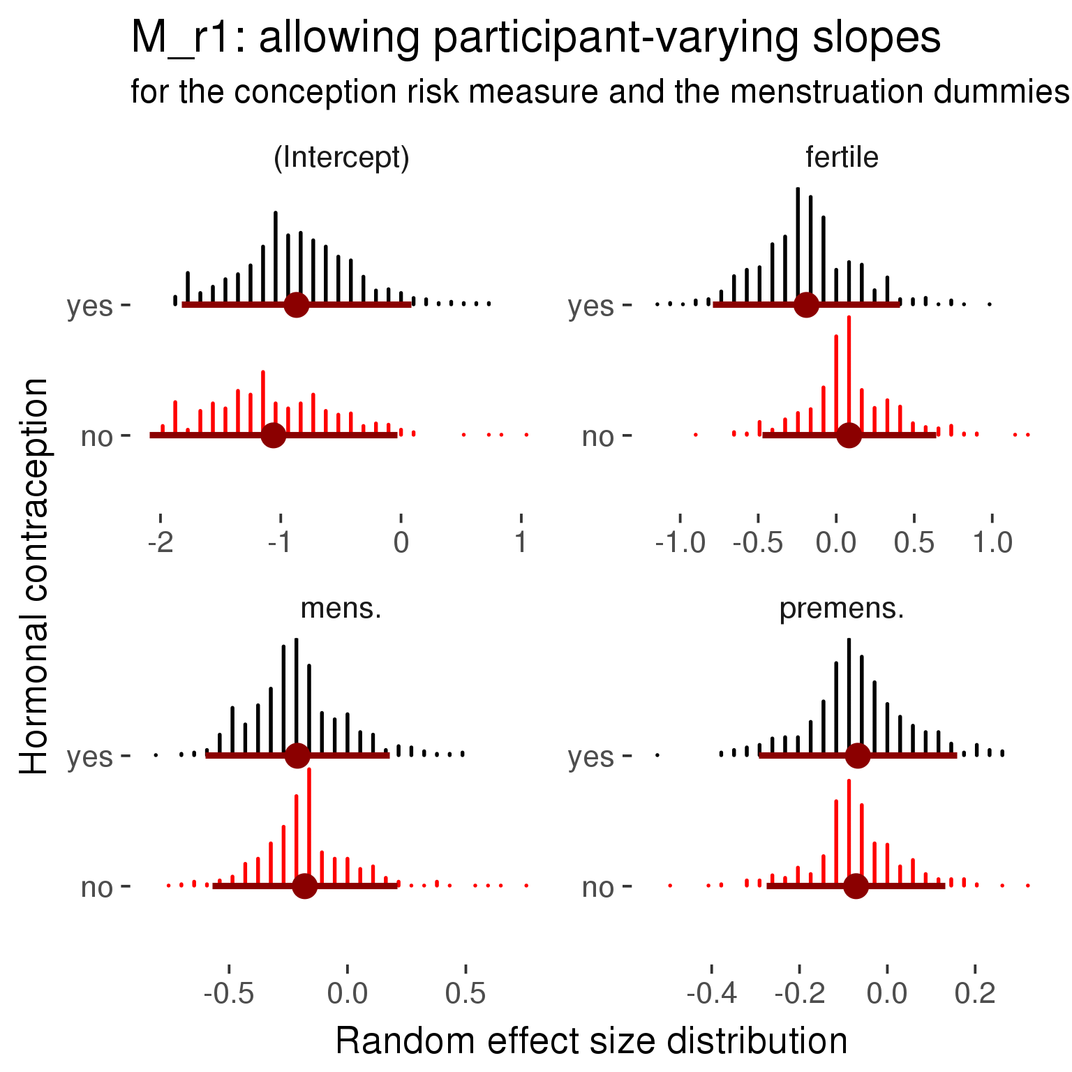
Generalized linear mixed model fit by maximum likelihood (Laplace Approximation) ['glmerMod']
Family: binomial ( probit )
Formula: had_petting ~ included + menstruation + fertile + fertile_mean +
(1 + fertile + menstruation | person) + included:menstruation + included:fertile
Data: diary
AIC BIC logLik deviance df.resid
24028 24184 -11995 23990 26684
Scaled residuals:
Min 1Q Median 3Q Max
-2.089 -0.488 -0.332 -0.170 4.797
Random effects:
Groups Name Variance Std.Dev. Corr
person (Intercept) 0.410 0.640
fertile 0.587 0.766 -0.21
menstruationpre 0.102 0.319 -0.22 0.74
menstruationyes 0.214 0.463 -0.17 0.05 0.41
Number of obs: 26703, groups: person, 1054
Fixed effects:
Estimate Std. Error z value Pr(>|z|)
(Intercept) -1.10079 0.07349 -14.98 < 2e-16 ***
includedhorm_contra 0.19832 0.05968 3.32 0.00089 ***
menstruationpre -0.07412 0.05903 -1.26 0.20929
menstruationyes -0.18797 0.06315 -2.98 0.00291 **
fertile 0.08073 0.11941 0.68 0.49901
fertile_mean -0.05684 0.33638 -0.17 0.86583
includedhorm_contra:menstruationpre 0.00453 0.06790 0.07 0.94676
includedhorm_contra:menstruationyes -0.02949 0.07269 -0.41 0.68500
includedhorm_contra:fertile -0.27399 0.13862 -1.98 0.04810 *
---
Signif. codes: 0 '***' 0.001 '**' 0.01 '*' 0.05 '.' 0.1 ' ' 1
Correlation of Fixed Effects:
(Intr) incld_ mnstrtnp mnstrtny fertil frtl_m inclddhrm_cntr:mnstrtnp
inclddhrm_c -0.495
menstrutnpr -0.313 0.346
menstrutnys -0.258 0.298 0.339
fertile -0.293 0.422 0.479 0.295
fertile_men -0.744 -0.037 0.005 -0.008 -0.110
inclddhrm_cntr:mnstrtnp 0.252 -0.446 -0.764 -0.271 -0.379 -0.011
inclddhrm_cntr:mnstrtny 0.213 -0.384 -0.272 -0.733 -0.227 -0.005 0.356
inclddhrm_cntr:f 0.276 -0.538 -0.377 -0.227 -0.766 0.021 0.497
inclddhrm_cntr:mnstrtny
inclddhrm_c
menstrutnpr
menstrutnys
fertile
fertile_men
inclddhrm_cntr:mnstrtnp
inclddhrm_cntr:mnstrtny
inclddhrm_cntr:f 0.295
convergence code: 0
Model failed to converge with max|grad| = 0.085386 (tol = 0.001, component 1)
| Df | AIC | BIC | logLik | deviance | Chisq | Chi Df | Pr(>Chisq) | |
|---|---|---|---|---|---|---|---|---|
| model | 10 | 24084 | 24166 | -12032 | 24064 | NA | NA | NA |
| with_ind_diff | 19 | 24028 | 24184 | -11995 | 23990 | 74.04 | 9 | 2.439e-12 |
robustness_check_ovu_shift(model, diary)M_e: Exclusion criteria
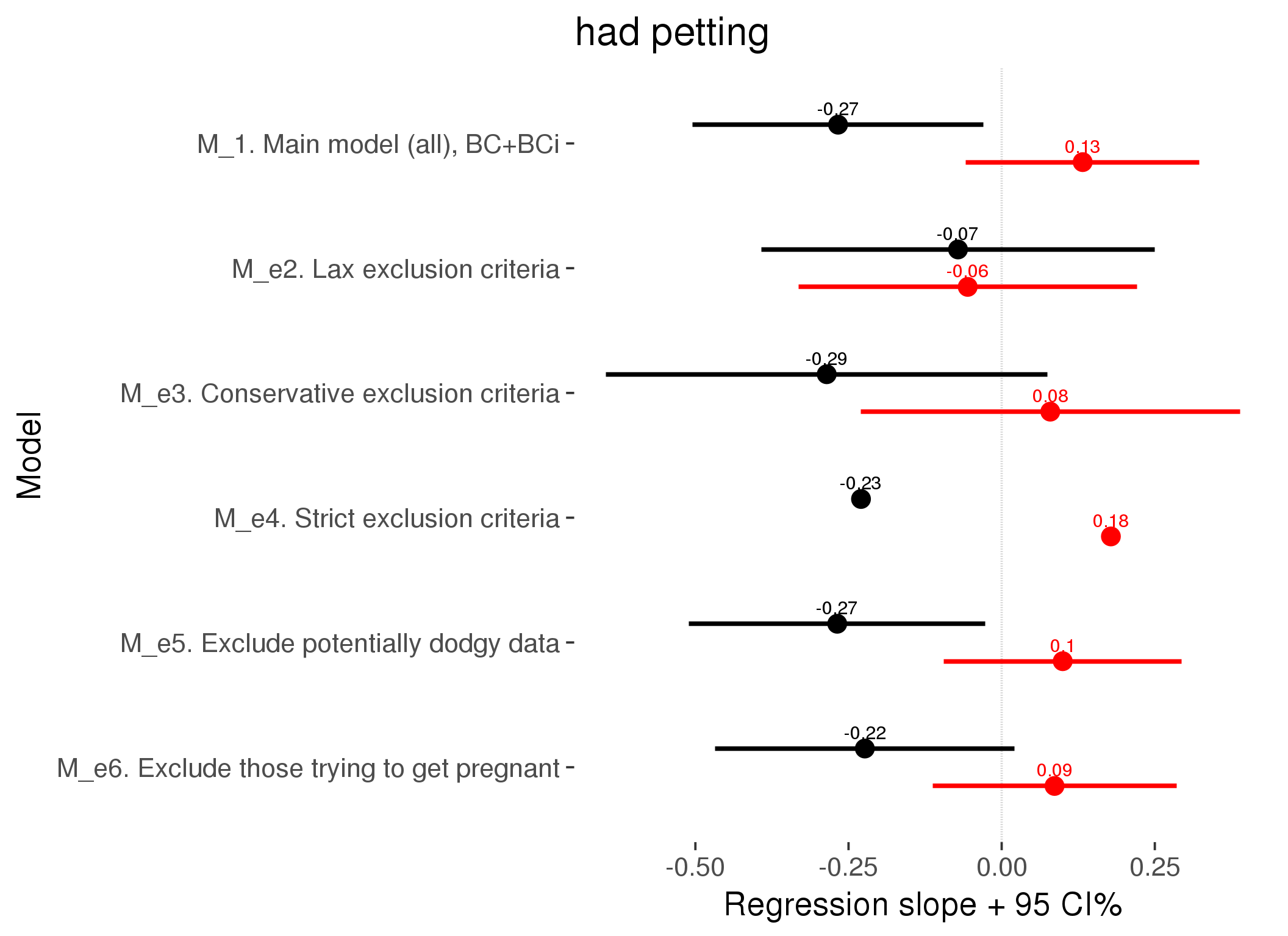
M_p: Predictors
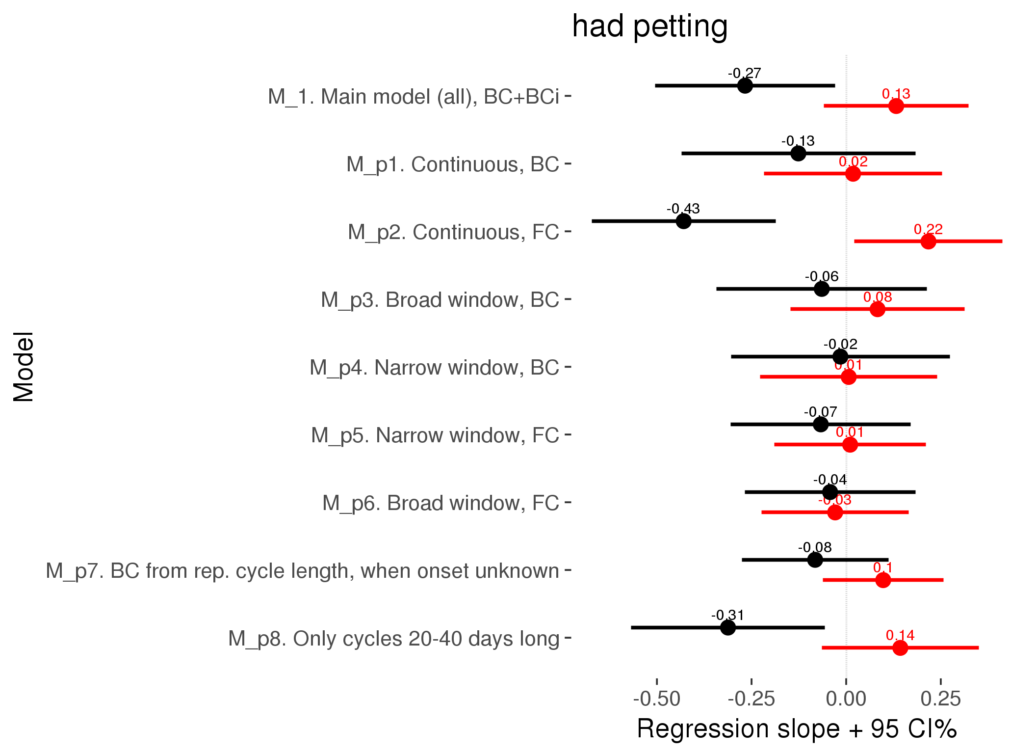
M_c: Covariates, controls, autocorrelation
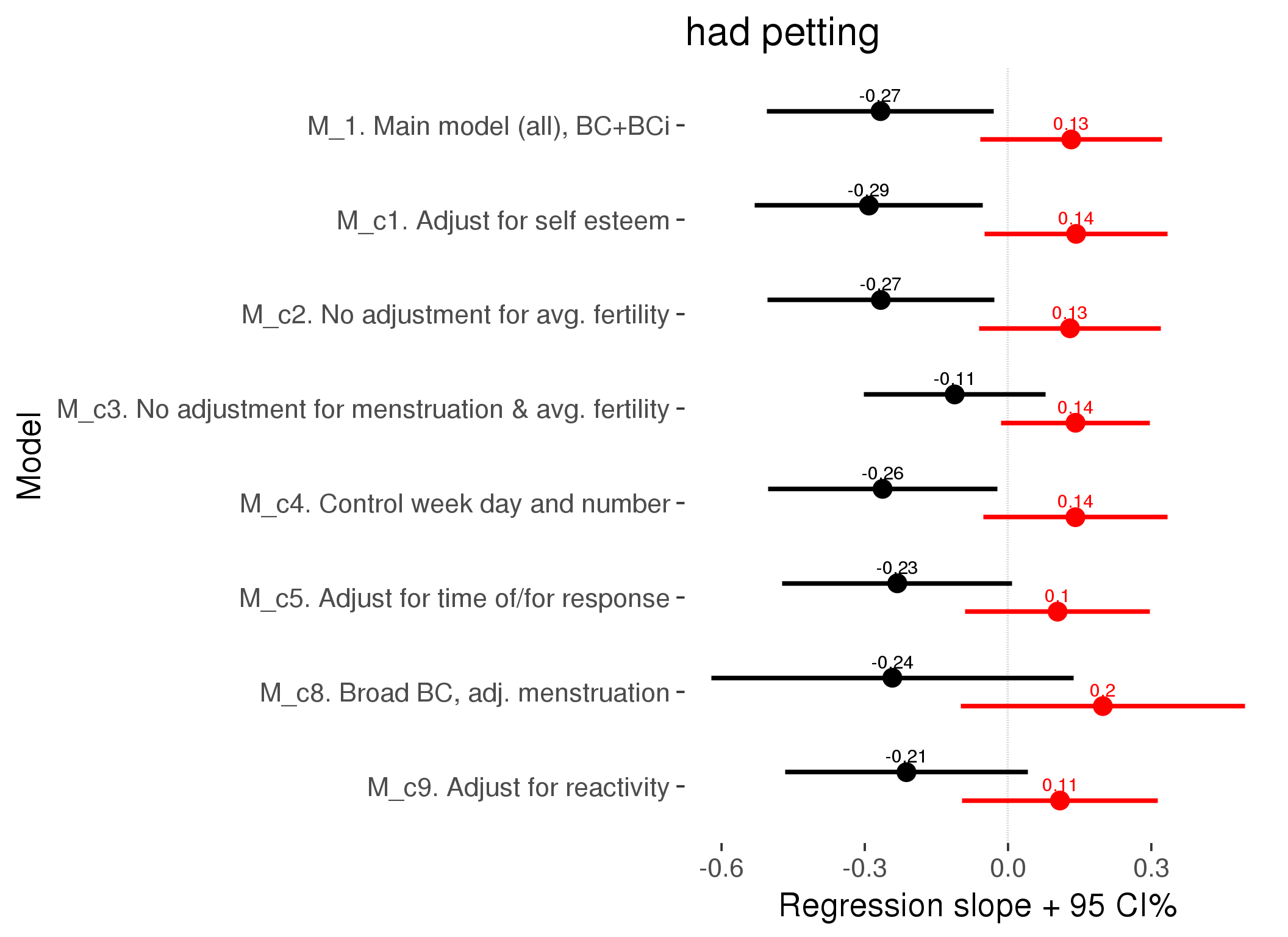
Generalized linear mixed model fit by maximum likelihood (Laplace Approximation) ['glmerMod']
Family: binomial ( probit )
AIC BIC logLik deviance df.resid
21797 21943 -10880 21761 24379
Scaled residuals:
Min 1Q Median 3Q Max
-1.980 -0.496 -0.336 -0.177 5.301
Random effects:
Groups Name Variance Std.Dev.
person (Intercept) 0.3683431348 0.606913
Xr.2 s(days_filled_out):includedhorm_contra 0.0000052021 0.002281
Xr.1 s(days_filled_out):includedcycling 0.0590677296 0.243039
Xr.0 s(day_number):includedhorm_contra 0.0000000339 0.000184
Xr s(day_number):includedcycling 0.0001816739 0.013479
Number of obs: 24397, groups: person, 1054; Xr.2, 8; Xr.1, 8; Xr.0, 8; Xr, 8
Fixed effects:
Estimate Std. Error z value Pr(>|z|)
X(Intercept) -1.11813 0.07175 -15.58 < 2e-16 ***
Xincludedhorm_contra 0.17193 0.05935 2.90 0.0038 **
Xmenstruationpre -0.04866 0.05141 -0.95 0.3439
Xmenstruationyes -0.11928 0.04982 -2.39 0.0166 *
Xfertile 0.10865 0.10432 1.04 0.2976
Xfertile_mean 0.02708 0.32861 0.08 0.9343
Xincludedhorm_contra:menstruationpre 0.00562 0.06449 0.09 0.9305
Xincludedhorm_contra:menstruationyes -0.04073 0.06395 -0.64 0.5242
Xincludedhorm_contra:fertile -0.21276 0.12976 -1.64 0.1011
Xs(day_number):includedcyclingFx1 0.29433 0.07353 4.00 0.000062559 ***
Xs(day_number):includedhorm_contraFx1 0.32977 0.05847 5.64 0.000000017 ***
Xs(days_filled_out):includedcyclingFx1 -0.12472 0.16653 -0.75 0.4539
Xs(days_filled_out):includedhorm_contraFx1 -0.31308 0.06005 -5.21 0.000000185 ***
---
Signif. codes: 0 '***' 0.001 '**' 0.01 '*' 0.05 '.' 0.1 ' ' 1
Family: binomial
Link function: probit
Formula:
had_petting ~ included + menstruation + fertile + fertile_mean +
s(day_number, by = included) + s(days_filled_out, by = included) +
included:menstruation + included:fertile
Parametric coefficients:
Estimate Std. Error z value Pr(>|z|)
(Intercept) -1.11813 0.06997 -15.98 <2e-16 ***
includedhorm_contra 0.17193 0.05840 2.94 0.0032 **
menstruationpre -0.04866 0.05063 -0.96 0.3365
menstruationyes -0.11928 0.04910 -2.43 0.0151 *
fertile 0.10865 0.10240 1.06 0.2887
fertile_mean 0.02708 0.32072 0.08 0.9327
includedhorm_contra:menstruationpre 0.00562 0.06353 0.09 0.9295
includedhorm_contra:menstruationyes -0.04073 0.06308 -0.65 0.5185
includedhorm_contra:fertile -0.21276 0.12750 -1.67 0.0952 .
---
Signif. codes: 0 '***' 0.001 '**' 0.01 '*' 0.05 '.' 0.1 ' ' 1
Approximate significance of smooth terms:
edf Ref.df Chi.sq p-value
s(day_number):includedcycling 1.01 1.01 17.3 0.0000335219 ***
s(day_number):includedhorm_contra 1.00 1.00 33.1 0.0000000089 ***
s(days_filled_out):includedcycling 2.87 2.87 20.8 0.00029 ***
s(days_filled_out):includedhorm_contra 1.00 1.00 28.2 0.0000001094 ***
---
Signif. codes: 0 '***' 0.001 '**' 0.01 '*' 0.05 '.' 0.1 ' ' 1
R-sq.(adj) = 0.0033
glmer.ML = 19644 Scale est. = 1 n = 24397
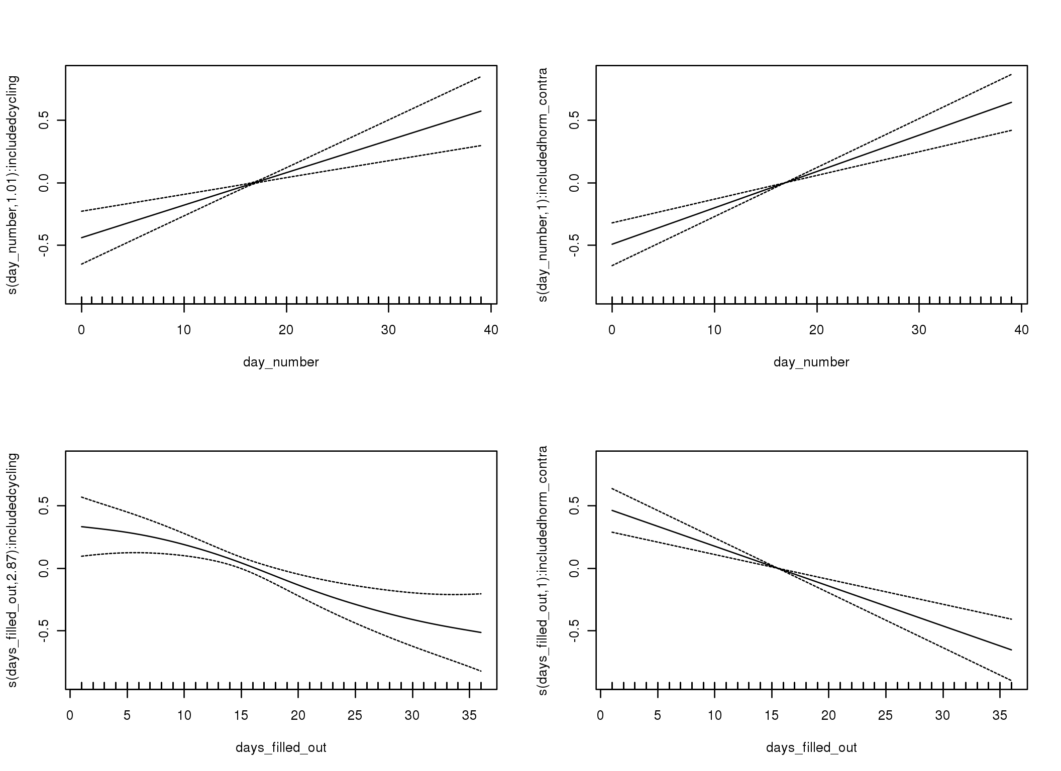
M_d: Other designs
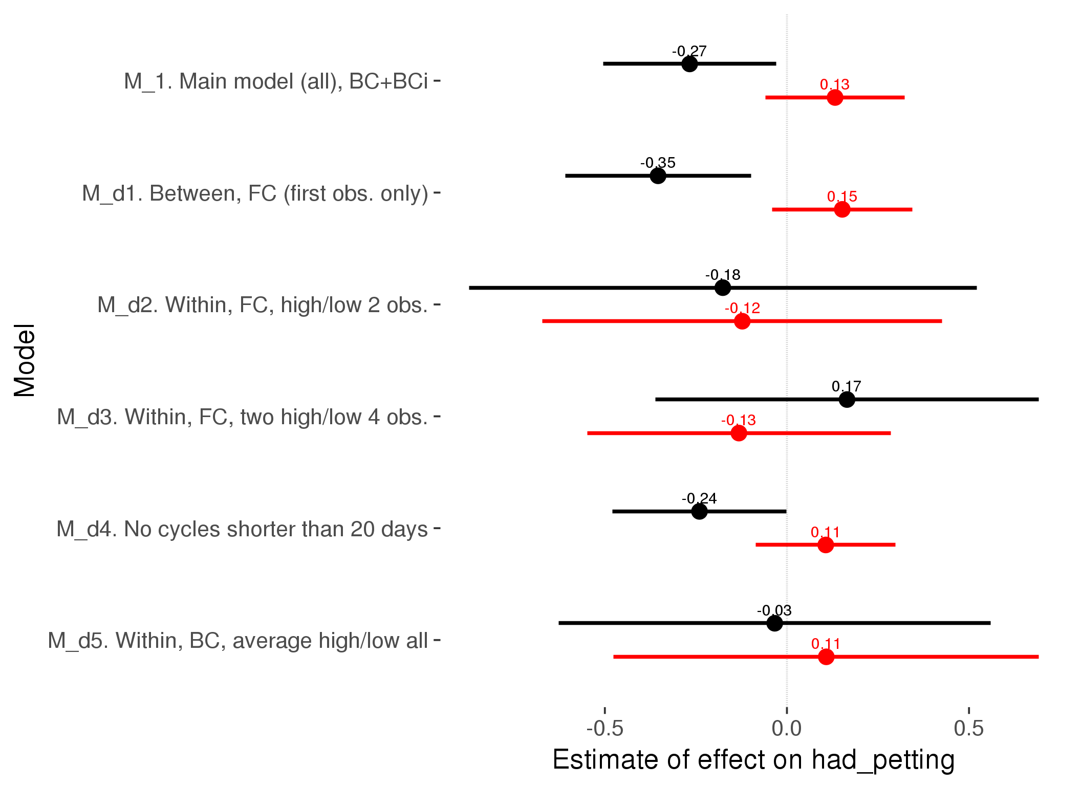
M_m1: Moderation by contraceptive method
Based on the sample with lax exclusion criteria. Users who used any hormonal contraception are classified as hormonal, users who use any awareness-based methods (counting, temperature-based) are classified as ‘fertility-awareness’, women who don’t fall into the before groups and use condoms, pessars, coitus interruptus etc. are classified as ‘barrie or abstinence’. Women who don’t use contraception or use other methods such as sterilisation are excluded from this analysis.
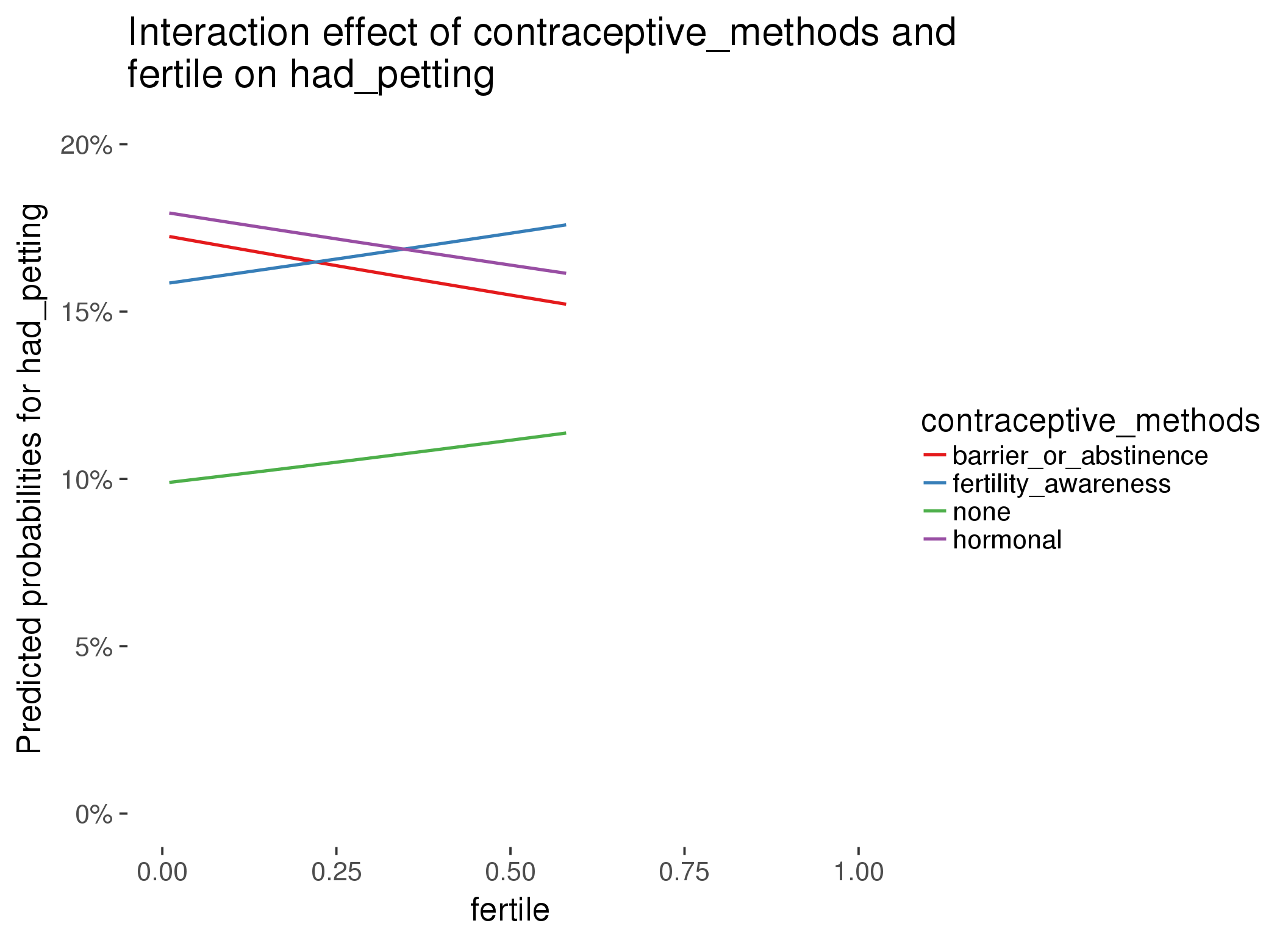
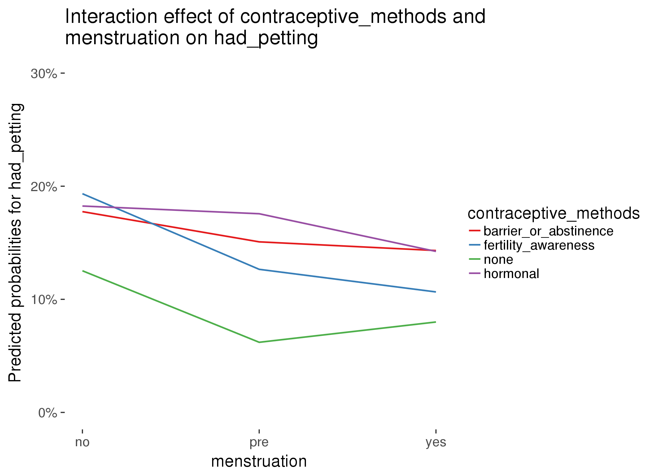
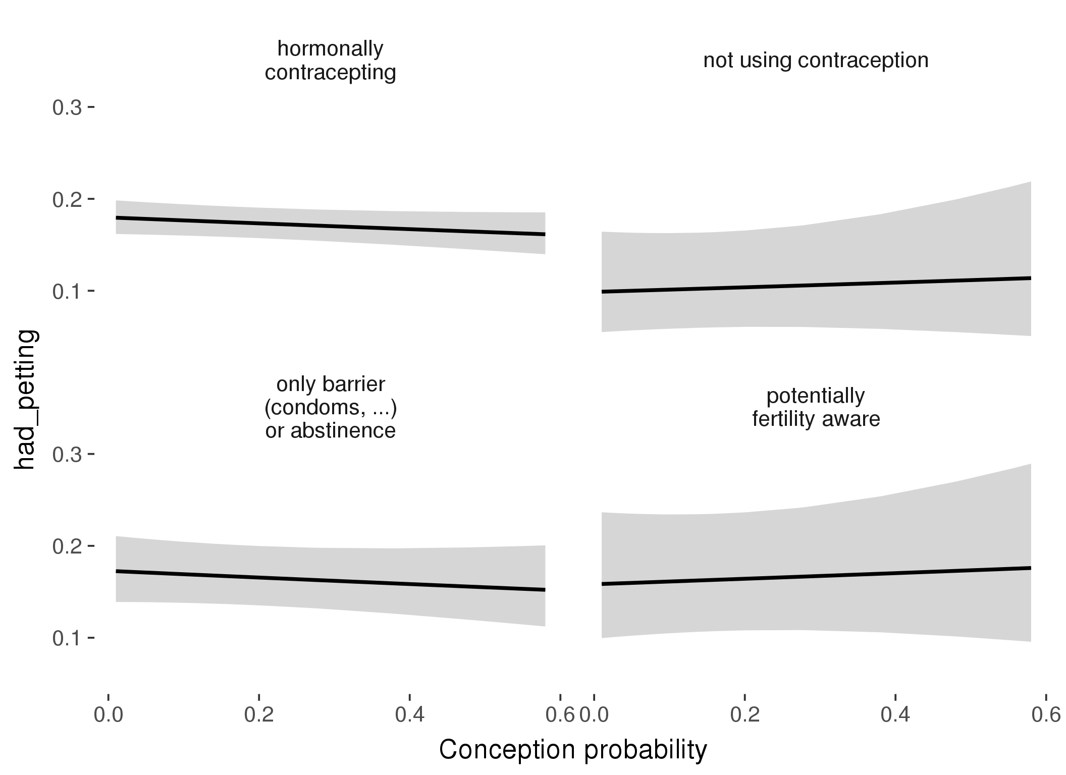
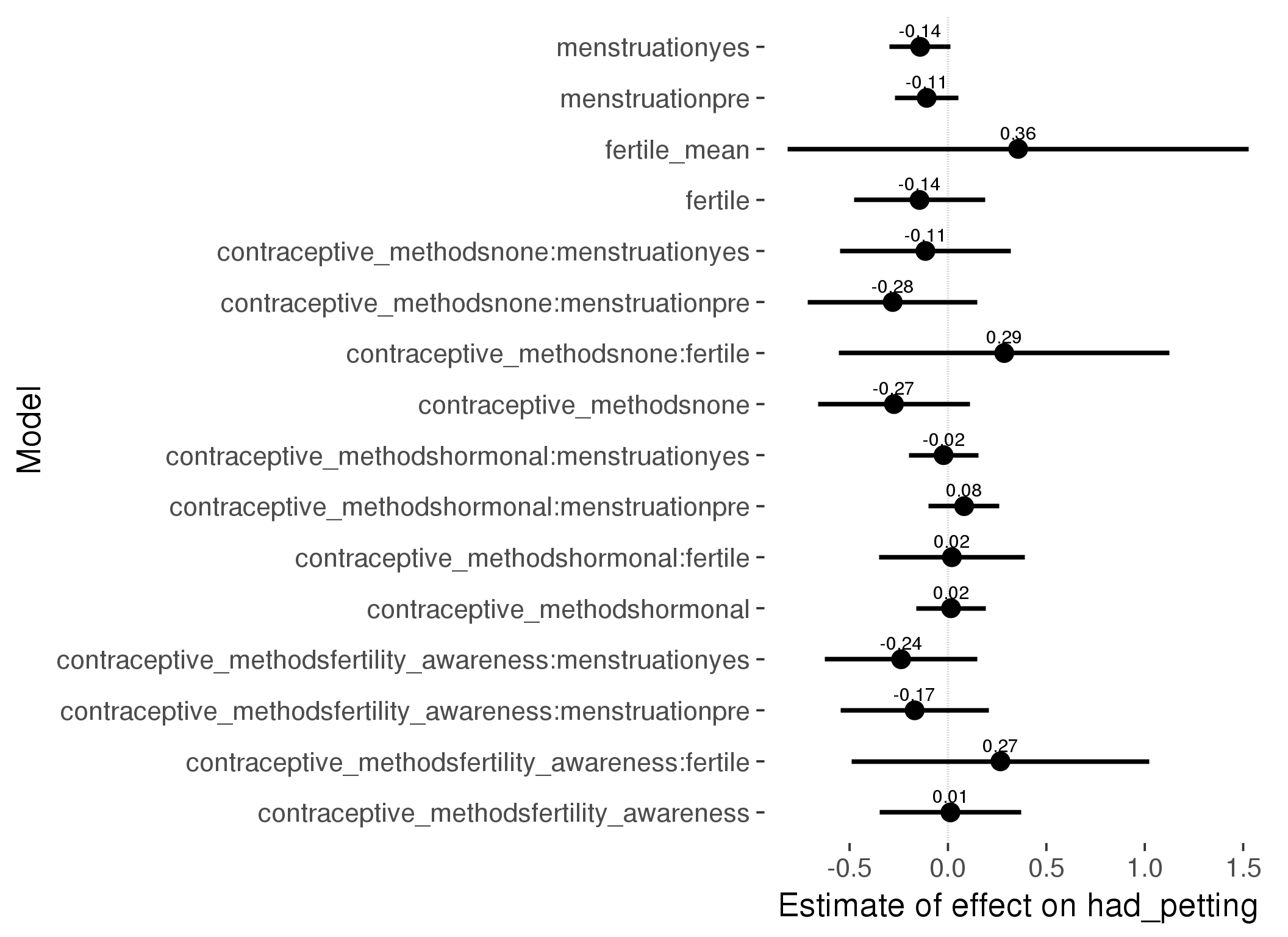
Generalized linear mixed model fit by maximum likelihood (Laplace Approximation) ['glmerMod']
Family: binomial ( probit )
Formula: had_petting ~ fertile_mean + (1 | person) + contraceptive_methods +
fertile + menstruation + fertile:contraceptive_methods + menstruation:contraceptive_methods
Data: diary
Subset: !is.na(included_lax) & contraceptive_method != "other"
AIC BIC logLik deviance df.resid
15891 16030 -7928 15855 17026
Scaled residuals:
Min 1Q Median 3Q Max
-2.009 -0.516 -0.368 -0.192 6.239
Random effects:
Groups Name Variance Std.Dev.
person (Intercept) 0.321 0.567
Number of obs: 17044, groups: person, 513
Fixed effects:
Estimate Std. Error z value Pr(>|z|)
(Intercept) -0.9620 0.1266 -7.60 2.9e-14 ***
fertile_mean 0.3564 0.5978 0.60 0.551
contraceptive_methodsfertility_awareness 0.0125 0.1832 0.07 0.946
contraceptive_methodsnone -0.2745 0.1969 -1.39 0.163
contraceptive_methodshormonal 0.0154 0.0901 0.17 0.865
fertile -0.1447 0.1697 -0.85 0.394
menstruationpre -0.1081 0.0816 -1.32 0.185
menstruationyes -0.1415 0.0789 -1.79 0.073 .
contraceptive_methodsfertility_awareness:fertile 0.2667 0.3852 0.69 0.489
contraceptive_methodsnone:fertile 0.2859 0.4289 0.67 0.505
contraceptive_methodshormonal:fertile 0.0199 0.1889 0.11 0.916
contraceptive_methodsfertility_awareness:menstruationpre -0.1694 0.1925 -0.88 0.379
contraceptive_methodsnone:menstruationpre -0.2808 0.2195 -1.28 0.201
contraceptive_methodshormonal:menstruationpre 0.0821 0.0917 0.90 0.371
contraceptive_methodsfertility_awareness:menstruationyes -0.2382 0.1973 -1.21 0.227
contraceptive_methodsnone:menstruationyes -0.1147 0.2209 -0.52 0.604
contraceptive_methodshormonal:menstruationyes -0.0223 0.0899 -0.25 0.804
---
Signif. codes: 0 '***' 0.001 '**' 0.01 '*' 0.05 '.' 0.1 ' ' 1
convergence code: 0
Model failed to converge with max|grad| = 0.128582 (tol = 0.001, component 1)
| Df | AIC | BIC | logLik | deviance | Chisq | Chi Df | Pr(>Chisq) | |
|---|---|---|---|---|---|---|---|---|
| add_main | 12 | 15886 | 15979 | -7931 | 15862 | NA | NA | NA |
| by_method | 18 | 15891 | 16030 | -7928 | 15855 | 7.422 | 6 | 0.2836 |
M_m2: Moderation by participant age
model %>%
test_moderator("age_group", diary, xlevels = 5)| Df | AIC | BIC | logLik | deviance | Chisq | Chi Df | Pr(>Chisq) | |
|---|---|---|---|---|---|---|---|---|
| with_main | 18 | 24034 | 24181 | -11999 | 23998 | NA | NA | NA |
| with_mod | 26 | 24046 | 24259 | -11997 | 23994 | 4.195 | 8 | 0.8391 |
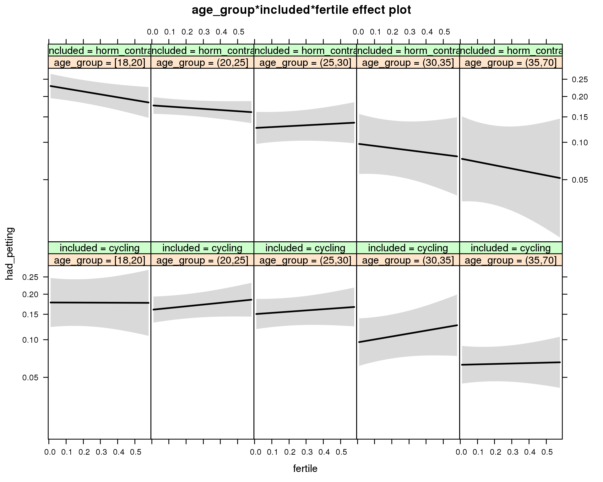
Generalized linear mixed model fit by maximum likelihood (Laplace Approximation) ['glmerMod']
Family: binomial ( probit )
Formula: had_petting ~ menstruation + fertile_mean + (1 | person) + age_group +
included + fertile + menstruation:included + age_group:included +
age_group:fertile + included:fertile + age_group:included:fertile
Data: diary
AIC BIC logLik deviance df.resid
24046 24259 -11997 23994 26677
Scaled residuals:
Min 1Q Median 3Q Max
-2.124 -0.502 -0.348 -0.175 5.750
Random effects:
Groups Name Variance Std.Dev.
person (Intercept) 0.344 0.587
Number of obs: 26703, groups: person, 1054
Fixed effects:
Estimate Std. Error z value Pr(>|z|)
(Intercept) -0.87810 0.13170 -6.67 0.000000000026 ***
menstruationpre -0.06328 0.04923 -1.29 0.1986
menstruationyes -0.12035 0.04666 -2.58 0.0099 **
fertile_mean -0.06693 0.31871 -0.21 0.8337
age_group(20,25] -0.07020 0.13699 -0.51 0.6084
age_group(25,30] -0.11221 0.14195 -0.79 0.4293
age_group(30,35] -0.38521 0.16835 -2.29 0.0221 *
age_group(35,70] -0.60156 0.15241 -3.95 0.000079111073 ***
includedhorm_contra 0.19097 0.13849 1.38 0.1679
fertile -0.00576 0.26873 -0.02 0.9829
menstruationpre:includedhorm_contra 0.00332 0.06171 0.05 0.9570
menstruationyes:includedhorm_contra -0.03710 0.05989 -0.62 0.5356
age_group(20,25]:includedhorm_contra -0.11941 0.15515 -0.77 0.4415
age_group(25,30]:includedhorm_contra -0.29555 0.17344 -1.70 0.0884 .
age_group(30,35]:includedhorm_contra -0.17468 0.23254 -0.75 0.4525
age_group(35,70]:includedhorm_contra -0.10118 0.26746 -0.38 0.7052
age_group(20,25]:fertile 0.17301 0.29575 0.58 0.5585
age_group(25,30]:fertile 0.12460 0.30675 0.41 0.6846
age_group(30,35]:fertile 0.29123 0.36910 0.79 0.4301
age_group(35,70]:fertile 0.04733 0.34373 0.14 0.8905
includedhorm_contra:fertile -0.27244 0.29601 -0.92 0.3574
age_group(20,25]:includedhorm_contra:fertile -0.00695 0.32981 -0.02 0.9832
age_group(25,30]:includedhorm_contra:fertile 0.24127 0.37010 0.65 0.5145
age_group(30,35]:includedhorm_contra:fertile -0.22350 0.51539 -0.43 0.6645
age_group(35,70]:includedhorm_contra:fertile -0.09399 0.63633 -0.15 0.8826
---
Signif. codes: 0 '***' 0.001 '**' 0.01 '*' 0.05 '.' 0.1 ' ' 1
convergence code: 0
Model failed to converge with max|grad| = 0.113113 (tol = 0.001, component 1)
M_m3: Moderation by weekend
model %>%
test_moderator("weekend", diary, xlevels = 2) | Df | AIC | BIC | logLik | deviance | Chisq | Chi Df | Pr(>Chisq) | |
|---|---|---|---|---|---|---|---|---|
| with_main | 12 | 23839 | 23937 | -11907 | 23815 | NA | NA | NA |
| with_mod | 14 | 23841 | 23956 | -11907 | 23813 | 1.397 | 2 | 0.4974 |
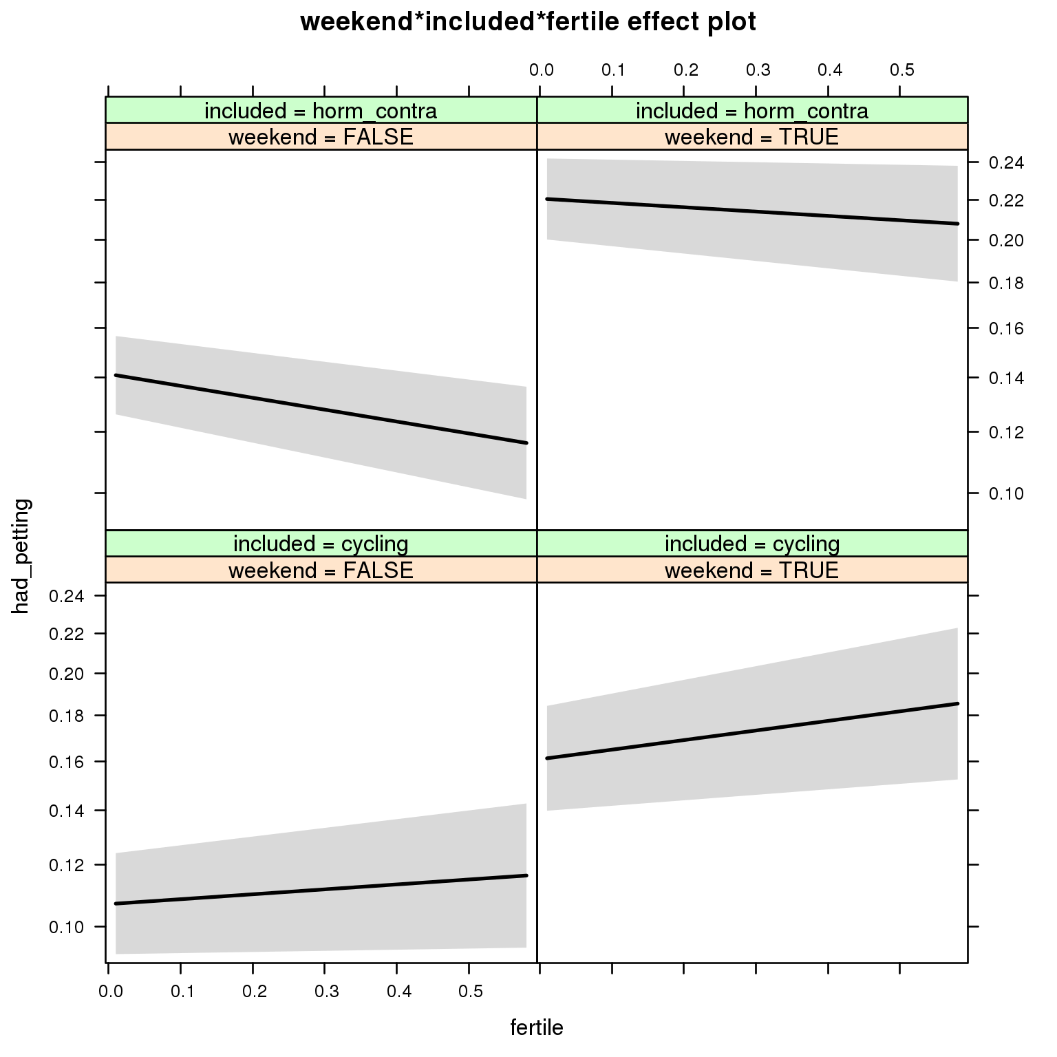
Generalized linear mixed model fit by maximum likelihood (Laplace Approximation) ['glmerMod']
Family: binomial ( probit )
Formula: had_petting ~ menstruation + fertile_mean + (1 | person) + weekend +
included + fertile + menstruation:included + weekend:included +
weekend:fertile + included:fertile + weekend:included:fertile
Data: diary
AIC BIC logLik deviance df.resid
23842 23956 -11907 23814 26689
Scaled residuals:
Min 1Q Median 3Q Max
-2.238 -0.495 -0.337 -0.167 5.871
Random effects:
Groups Name Variance Std.Dev.
person (Intercept) 0.378 0.615
Number of obs: 26703, groups: person, 1054
Fixed effects:
Estimate Std. Error z value Pr(>|z|)
(Intercept) -1.19928 0.07308 -16.41 < 2e-16 ***
menstruationpre -0.06604 0.04943 -1.34 0.1816
menstruationyes -0.12373 0.04678 -2.65 0.0082 **
fertile_mean -0.05984 0.32675 -0.18 0.8547
weekendTRUE 0.25181 0.04284 5.88 0.0000000041 ***
includedhorm_contra 0.17279 0.06238 2.77 0.0056 **
fertile 0.08560 0.12288 0.70 0.4860
menstruationpre:includedhorm_contra 0.00553 0.06200 0.09 0.9289
menstruationyes:includedhorm_contra -0.03159 0.06013 -0.53 0.5994
weekendTRUE:includedhorm_contra 0.05315 0.05392 0.99 0.3243
weekendTRUE:fertile 0.08114 0.16299 0.50 0.6186
includedhorm_contra:fertile -0.29233 0.15422 -1.90 0.0580 .
weekendTRUE:includedhorm_contra:fertile 0.05026 0.20462 0.25 0.8060
---
Signif. codes: 0 '***' 0.001 '**' 0.01 '*' 0.05 '.' 0.1 ' ' 1
convergence code: 0
Model failed to converge with max|grad| = 0.0214221 (tol = 0.001, component 1)
M_m4: Moderation by weekday
model %>%
test_moderator("weekday", diary, xlevels = 7)| Df | AIC | BIC | logLik | deviance | Chisq | Chi Df | Pr(>Chisq) | |
|---|---|---|---|---|---|---|---|---|
| with_main | 22 | 23633 | 23813 | -11794 | 23589 | NA | NA | NA |
| with_mod | 34 | 23648 | 23926 | -11790 | 23580 | 9.025 | 12 | 0.7008 |
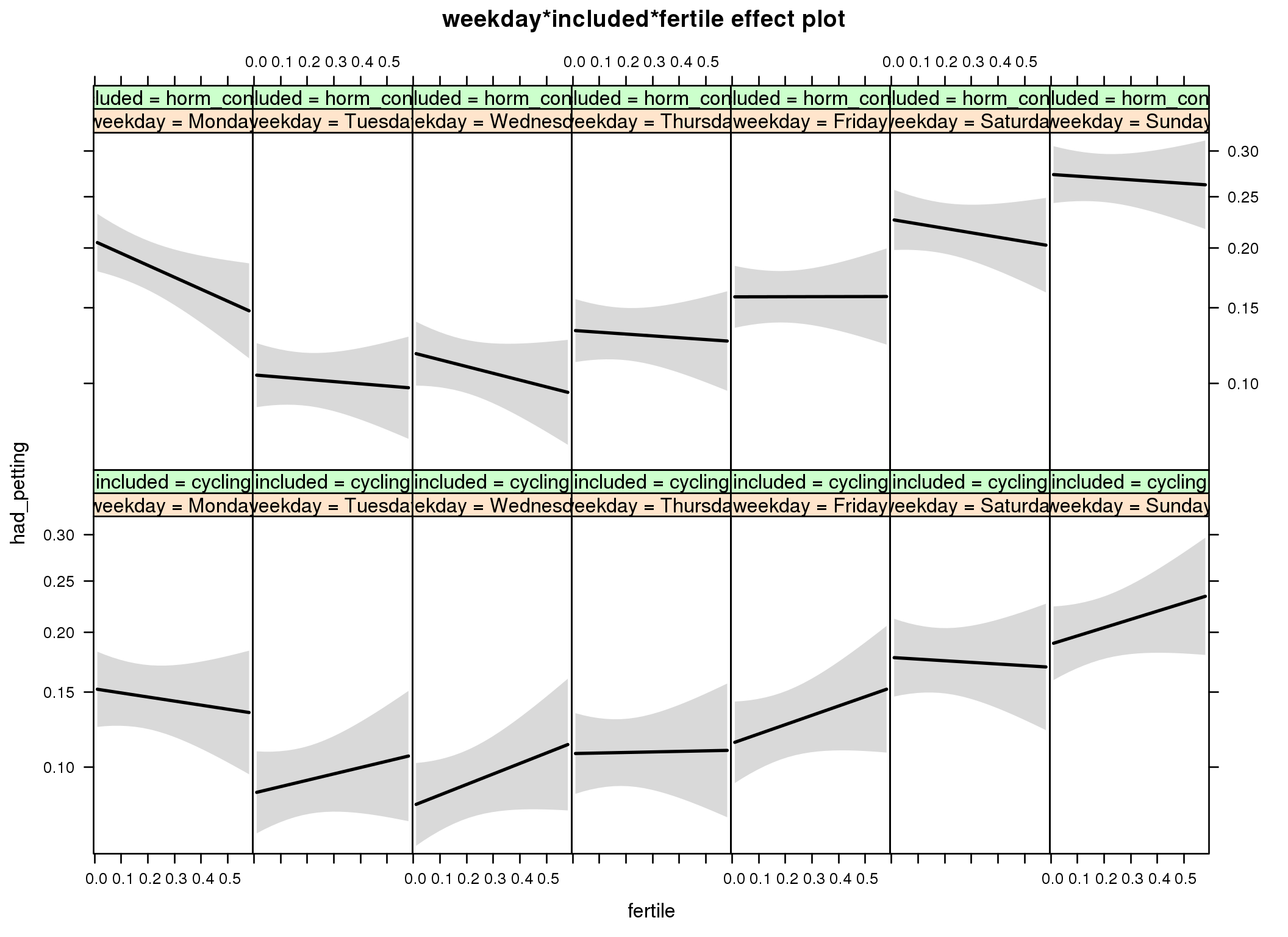
Generalized linear mixed model fit by maximum likelihood (Laplace Approximation) ['glmerMod']
Family: binomial ( probit )
Formula: had_petting ~ menstruation + fertile_mean + (1 | person) + weekday +
included + fertile + menstruation:included + weekday:included +
weekday:fertile + included:fertile + weekday:included:fertile
Data: diary
AIC BIC logLik deviance df.resid
23648 23926 -11790 23580 26669
Scaled residuals:
Min 1Q Median 3Q Max
-2.537 -0.490 -0.327 -0.161 6.512
Random effects:
Groups Name Variance Std.Dev.
person (Intercept) 0.388 0.623
Number of obs: 26703, groups: person, 1054
Fixed effects:
Estimate Std. Error z value Pr(>|z|)
(Intercept) -0.97802 0.08636 -11.33 < 2e-16 ***
menstruationpre -0.06737 0.04974 -1.35 0.1756
menstruationyes -0.12518 0.04702 -2.66 0.0078 **
fertile_mean -0.08049 0.33058 -0.24 0.8076
weekdayTuesday -0.33915 0.07967 -4.26 0.0000207 ***
weekdayWednesday -0.37980 0.08029 -4.73 0.0000022 ***
weekdayThursday -0.21073 0.07886 -2.67 0.0075 **
weekdayFriday -0.17709 0.07939 -2.23 0.0257 *
weekdaySaturday 0.10223 0.07685 1.33 0.1834
weekdaySunday 0.14595 0.07378 1.98 0.0479 *
includedhorm_contra 0.20979 0.08412 2.49 0.0126 *
fertile -0.13265 0.21385 -0.62 0.5351
menstruationpre:includedhorm_contra 0.00763 0.06241 0.12 0.9028
menstruationyes:includedhorm_contra -0.02685 0.06047 -0.44 0.6570
weekdayTuesday:includedhorm_contra -0.09594 0.10064 -0.95 0.3405
weekdayWednesday:includedhorm_contra 0.01629 0.10113 0.16 0.8720
weekdayThursday:includedhorm_contra -0.07927 0.09957 -0.80 0.4260
weekdayFriday:includedhorm_contra -0.00358 0.09953 -0.04 0.9713
weekdaySaturday:includedhorm_contra -0.03093 0.09674 -0.32 0.7492
weekdaySunday:includedhorm_contra 0.07223 0.09287 0.78 0.4367
weekdayTuesday:fertile 0.34004 0.30466 1.12 0.2644
weekdayWednesday:fertile 0.47471 0.30690 1.55 0.1219
weekdayThursday:fertile 0.15038 0.30813 0.49 0.6255
weekdayFriday:fertile 0.43594 0.30103 1.45 0.1476
weekdaySaturday:fertile 0.07961 0.29695 0.27 0.7886
weekdaySunday:fertile 0.40094 0.28421 1.41 0.1583
includedhorm_contra:fertile -0.25726 0.26897 -0.96 0.3388
weekdayTuesday:includedhorm_contra:fertile -0.02203 0.38584 -0.06 0.9545
weekdayWednesday:includedhorm_contra:fertile -0.30586 0.38958 -0.79 0.4324
weekdayThursday:includedhorm_contra:fertile 0.17989 0.38633 0.47 0.6415
weekdayFriday:includedhorm_contra:fertile -0.04421 0.37789 -0.12 0.9069
weekdaySaturday:includedhorm_contra:fertile 0.16628 0.37261 0.45 0.6554
weekdaySunday:includedhorm_contra:fertile -0.06921 0.35756 -0.19 0.8465
---
Signif. codes: 0 '***' 0.001 '**' 0.01 '*' 0.05 '.' 0.1 ' ' 1
convergence code: 0
Model failed to converge with max|grad| = 0.0978872 (tol = 0.001, component 1)
failure to converge in 10000 evaluations
M_m5: Moderation by exclusion threshold
model %>%
test_moderator("included_levels", diary, xlevels = 4)| Df | AIC | BIC | logLik | deviance | Chisq | Chi Df | Pr(>Chisq) | |
|---|---|---|---|---|---|---|---|---|
| with_main | 16 | 24090 | 24221 | -12029 | 24058 | NA | NA | NA |
| with_mod | 22 | 24098 | 24278 | -12027 | 24054 | 4.323 | 6 | 0.633 |
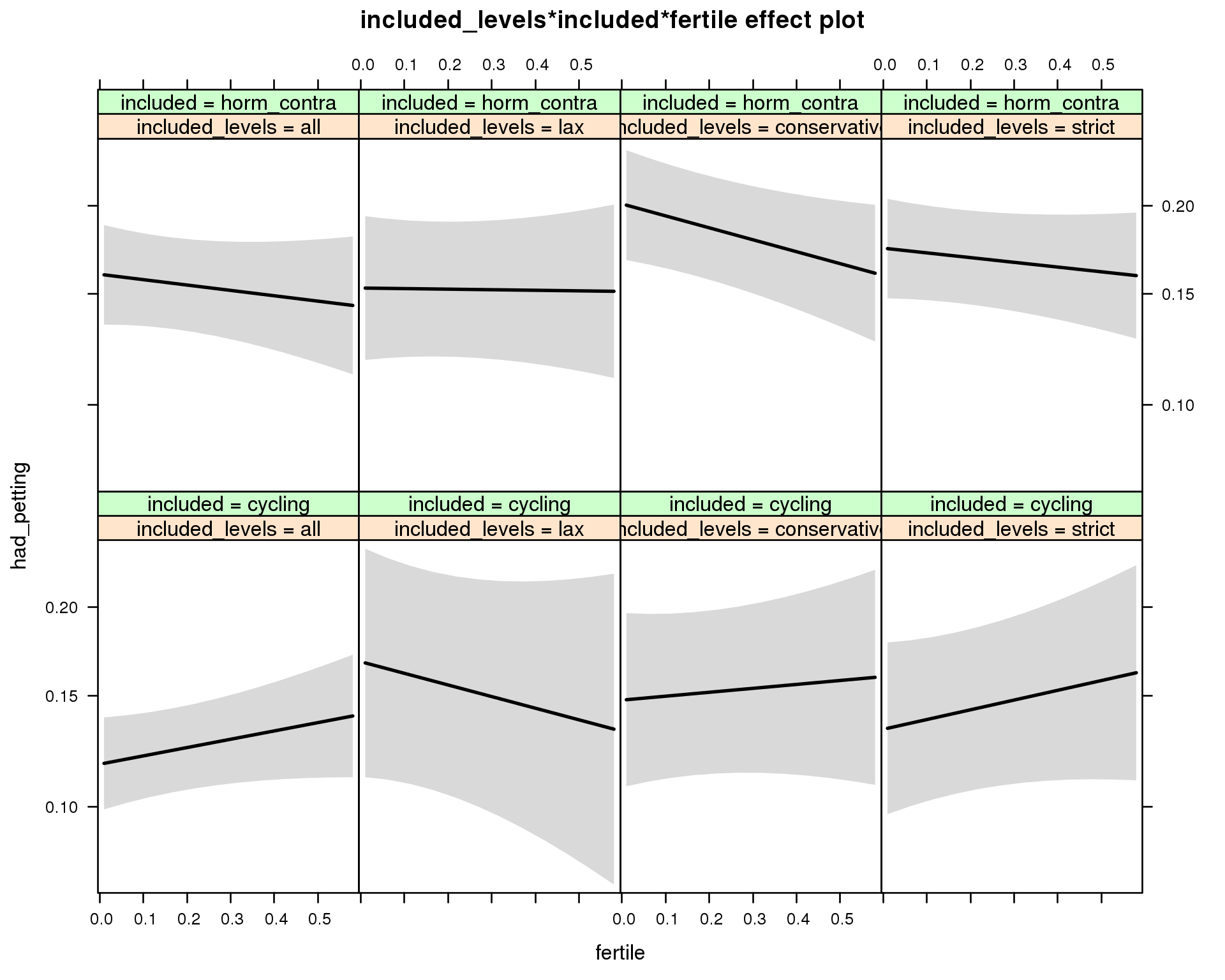
Generalized linear mixed model fit by maximum likelihood (Laplace Approximation) ['glmerMod']
Family: binomial ( probit )
Formula: had_petting ~ menstruation + fertile_mean + (1 | person) + included_levels +
included + fertile + menstruation:included + included_levels:included +
included_levels:fertile + included:fertile + included_levels:included:fertile
Data: diary
AIC BIC logLik deviance df.resid
24098 24278 -12027 24054 26681
Scaled residuals:
Min 1Q Median 3Q Max
-2.324 -0.499 -0.346 -0.177 5.283
Random effects:
Groups Name Variance Std.Dev.
person (Intercept) 0.367 0.606
Number of obs: 26703, groups: person, 1054
Fixed effects:
Estimate Std. Error z value Pr(>|z|)
(Intercept) -1.14019 0.07797 -14.62 <2e-16 ***
menstruationpre -0.06518 0.04922 -1.32 0.1855
menstruationyes -0.12079 0.04663 -2.59 0.0096 **
fertile_mean -0.08633 0.32945 -0.26 0.7933
included_levelslax 0.22612 0.13887 1.63 0.1034
included_levelsconservative 0.14143 0.11022 1.28 0.1994
included_levelsstrict 0.07705 0.10941 0.70 0.4813
includedhorm_contra 0.19946 0.08009 2.49 0.0128 *
fertile 0.18357 0.12491 1.47 0.1417
menstruationpre:includedhorm_contra 0.00716 0.06175 0.12 0.9077
menstruationyes:includedhorm_contra -0.03498 0.05992 -0.58 0.5594
included_levelslax:includedhorm_contra -0.25648 0.17088 -1.50 0.1334
included_levelsconservative:includedhorm_contra 0.01382 0.13838 0.10 0.9204
included_levelsstrict:includedhorm_contra -0.01937 0.13511 -0.14 0.8860
included_levelslax:fertile -0.44006 0.30450 -1.45 0.1484
included_levelsconservative:fertile -0.09688 0.22129 -0.44 0.6615
included_levelsstrict:fertile 0.03155 0.22378 0.14 0.8879
includedhorm_contra:fertile -0.30211 0.18608 -1.62 0.1045
included_levelslax:includedhorm_contra:fertile 0.54623 0.36643 1.49 0.1360
included_levelsconservative:includedhorm_contra:fertile -0.04823 0.28534 -0.17 0.8658
included_levelsstrict:includedhorm_contra:fertile -0.01740 0.28351 -0.06 0.9511
---
Signif. codes: 0 '***' 0.001 '**' 0.01 '*' 0.05 '.' 0.1 ' ' 1
convergence code: 0
Model failed to converge with max|grad| = 0.023207 (tol = 0.001, component 1)
M_m6: Moderation by cycle length
model %>%
test_moderator("cycle_length_groups", diary, xlevels = 4)| Df | AIC | BIC | logLik | deviance | Chisq | Chi Df | Pr(>Chisq) | |
|---|---|---|---|---|---|---|---|---|
| with_main | 16 | 24092 | 24223 | -12030 | 24060 | NA | NA | NA |
| with_mod | 22 | 24102 | 24282 | -12029 | 24058 | 1.852 | 6 | 0.9328 |
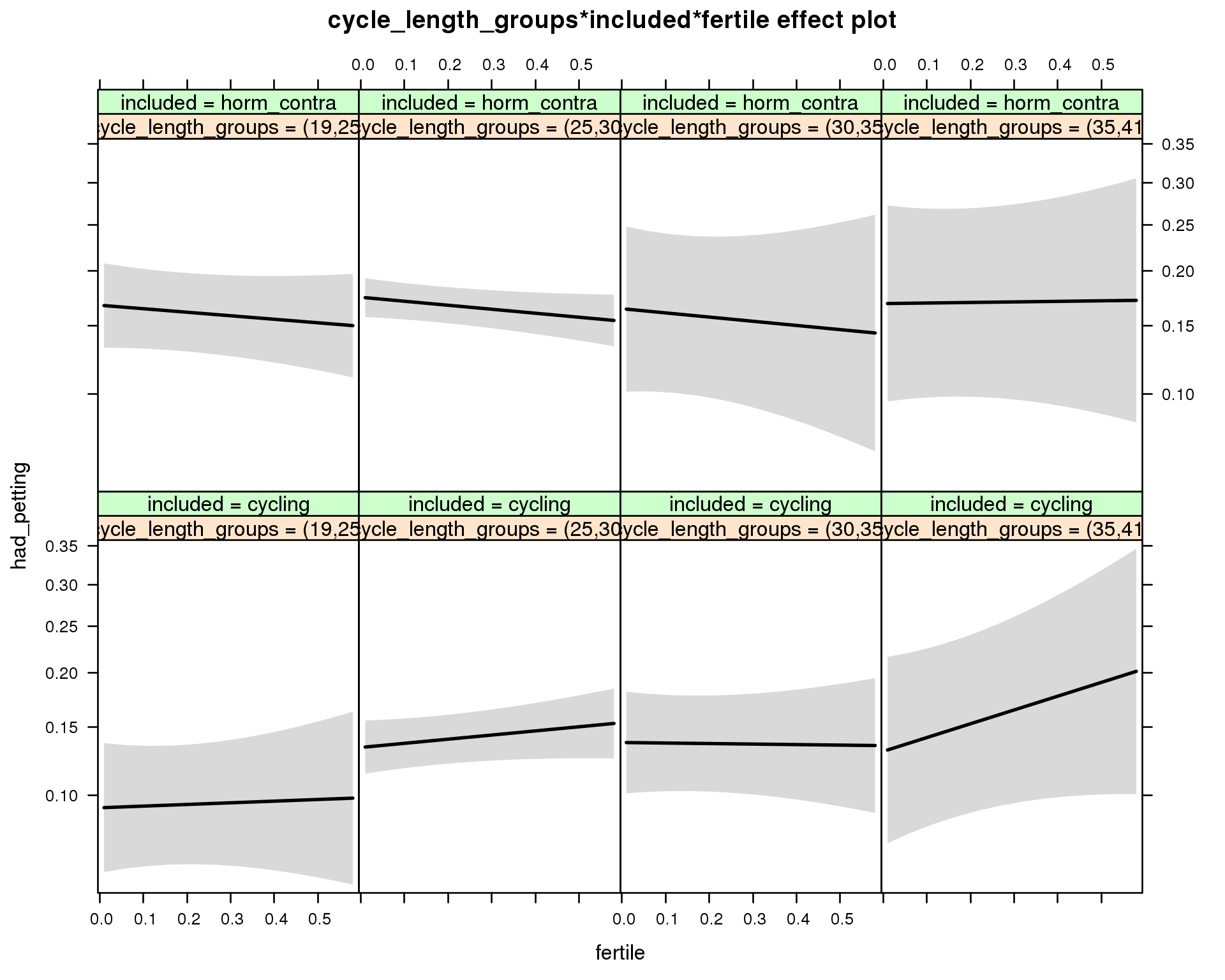
Generalized linear mixed model fit by maximum likelihood (Laplace Approximation) ['glmerMod']
Family: binomial ( probit )
Formula: had_petting ~ menstruation + fertile_mean + (1 | person) + cycle_length_groups +
included + fertile + menstruation:included + cycle_length_groups:included +
cycle_length_groups:fertile + included:fertile + cycle_length_groups:included:fertile
Data: diary
AIC BIC logLik deviance df.resid
24102 24282 -12029 24058 26681
Scaled residuals:
Min 1Q Median 3Q Max
-2.289 -0.499 -0.348 -0.176 5.367
Random effects:
Groups Name Variance Std.Dev.
person (Intercept) 0.368 0.606
Number of obs: 26703, groups: person, 1054
Fixed effects:
Estimate Std. Error z value Pr(>|z|)
(Intercept) -1.28410 0.13182 -9.74 <2e-16 ***
menstruationpre -0.06370 0.04925 -1.29 0.196
menstruationyes -0.11879 0.04691 -2.53 0.011 *
fertile_mean -0.05670 0.32735 -0.17 0.862
cycle_length_groups(25,30] 0.21661 0.12790 1.69 0.090 .
cycle_length_groups(30,35] 0.23434 0.15065 1.56 0.120
cycle_length_groups(35,41] 0.20256 0.20847 0.97 0.331
includedhorm_contra 0.36704 0.14408 2.55 0.011 *
fertile 0.05961 0.28010 0.21 0.831
menstruationpre:includedhorm_contra 0.00753 0.06174 0.12 0.903
menstruationyes:includedhorm_contra -0.03632 0.06017 -0.60 0.546
cycle_length_groups(25,30]:includedhorm_contra -0.18806 0.15366 -1.22 0.221
cycle_length_groups(30,35]:includedhorm_contra -0.24691 0.22768 -1.08 0.278
cycle_length_groups(35,41]:includedhorm_contra -0.19666 0.28605 -0.69 0.492
cycle_length_groups(25,30]:fertile 0.08890 0.29688 0.30 0.765
cycle_length_groups(30,35]:fertile -0.07826 0.34428 -0.23 0.820
cycle_length_groups(35,41]:fertile 0.43579 0.45928 0.95 0.343
includedhorm_contra:fertile -0.18578 0.32114 -0.58 0.563
cycle_length_groups(25,30]:includedhorm_contra:fertile -0.10611 0.34230 -0.31 0.757
cycle_length_groups(30,35]:includedhorm_contra:fertile 0.05422 0.51762 0.10 0.917
cycle_length_groups(35,41]:includedhorm_contra:fertile -0.28973 0.59062 -0.49 0.624
---
Signif. codes: 0 '***' 0.001 '**' 0.01 '*' 0.05 '.' 0.1 ' ' 1
convergence code: 0
Model failed to converge with max|grad| = 0.0868976 (tol = 0.001, component 1)
M_m7: Moderation by certainty about menstruation parameters
model %>%
test_moderator("certainty_menstruation", diary)| Df | AIC | BIC | logLik | deviance | Chisq | Chi Df | Pr(>Chisq) | |
|---|---|---|---|---|---|---|---|---|
| with_main | 12 | 24088 | 24186 | -12032 | 24064 | NA | NA | NA |
| with_mod | 14 | 24089 | 24204 | -12031 | 24061 | 2.543 | 2 | 0.2804 |
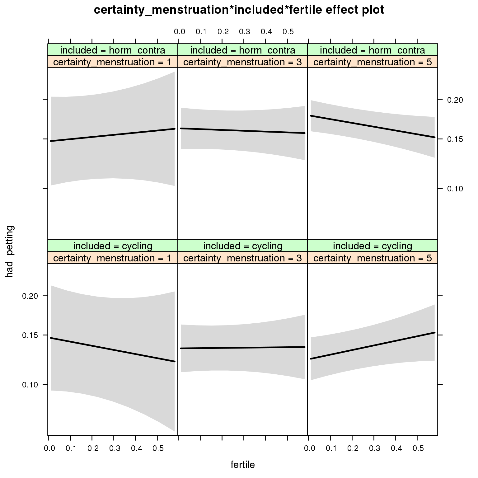
Generalized linear mixed model fit by maximum likelihood (Laplace Approximation) ['glmerMod']
Family: binomial ( probit )
Formula: had_petting ~ menstruation + fertile_mean + (1 | person) + certainty_menstruation +
included + fertile + menstruation:included + certainty_menstruation:included +
certainty_menstruation:fertile + included:fertile + certainty_menstruation:included:fertile
Data: diary
AIC BIC logLik deviance df.resid
24089 24204 -12031 24061 26689
Scaled residuals:
Min 1Q Median 3Q Max
-2.252 -0.499 -0.347 -0.176 5.452
Random effects:
Groups Name Variance Std.Dev.
person (Intercept) 0.368 0.607
Number of obs: 26703, groups: person, 1054
Fixed effects:
Estimate Std. Error z value Pr(>|z|)
(Intercept) -0.97839 0.18070 -5.41 0.000000062 ***
menstruationpre -0.05774 0.04916 -1.17 0.240
menstruationyes -0.11878 0.04666 -2.55 0.011 *
fertile_mean -0.07458 0.32385 -0.23 0.818
certainty_menstruation -0.02692 0.04117 -0.65 0.513
includedhorm_contra -0.05120 0.22748 -0.23 0.822
fertile -0.31313 0.38919 -0.80 0.421
menstruationpre:includedhorm_contra 0.00054 0.06165 0.01 0.993
menstruationyes:includedhorm_contra -0.03653 0.05990 -0.61 0.542
certainty_menstruation:includedhorm_contra 0.05907 0.05284 1.12 0.264
certainty_menstruation:fertile 0.10827 0.09113 1.19 0.235
includedhorm_contra:fertile 0.49346 0.49573 1.00 0.320
certainty_menstruation:includedhorm_contra:fertile -0.18189 0.11462 -1.59 0.113
---
Signif. codes: 0 '***' 0.001 '**' 0.01 '*' 0.05 '.' 0.1 ' ' 1
convergence code: 0
Model failed to converge with max|grad| = 0.33997 (tol = 0.001, component 1)
M_m8: Moderation by cycle regularity
model %>%
test_moderator("cycle_regularity", diary)| Df | AIC | BIC | logLik | deviance | Chisq | Chi Df | Pr(>Chisq) | |
|---|---|---|---|---|---|---|---|---|
| with_main | 14 | 24092 | 24206 | -12032 | 24064 | NA | NA | NA |
| with_mod | 18 | 24098 | 24246 | -12031 | 24062 | 1.335 | 4 | 0.8554 |
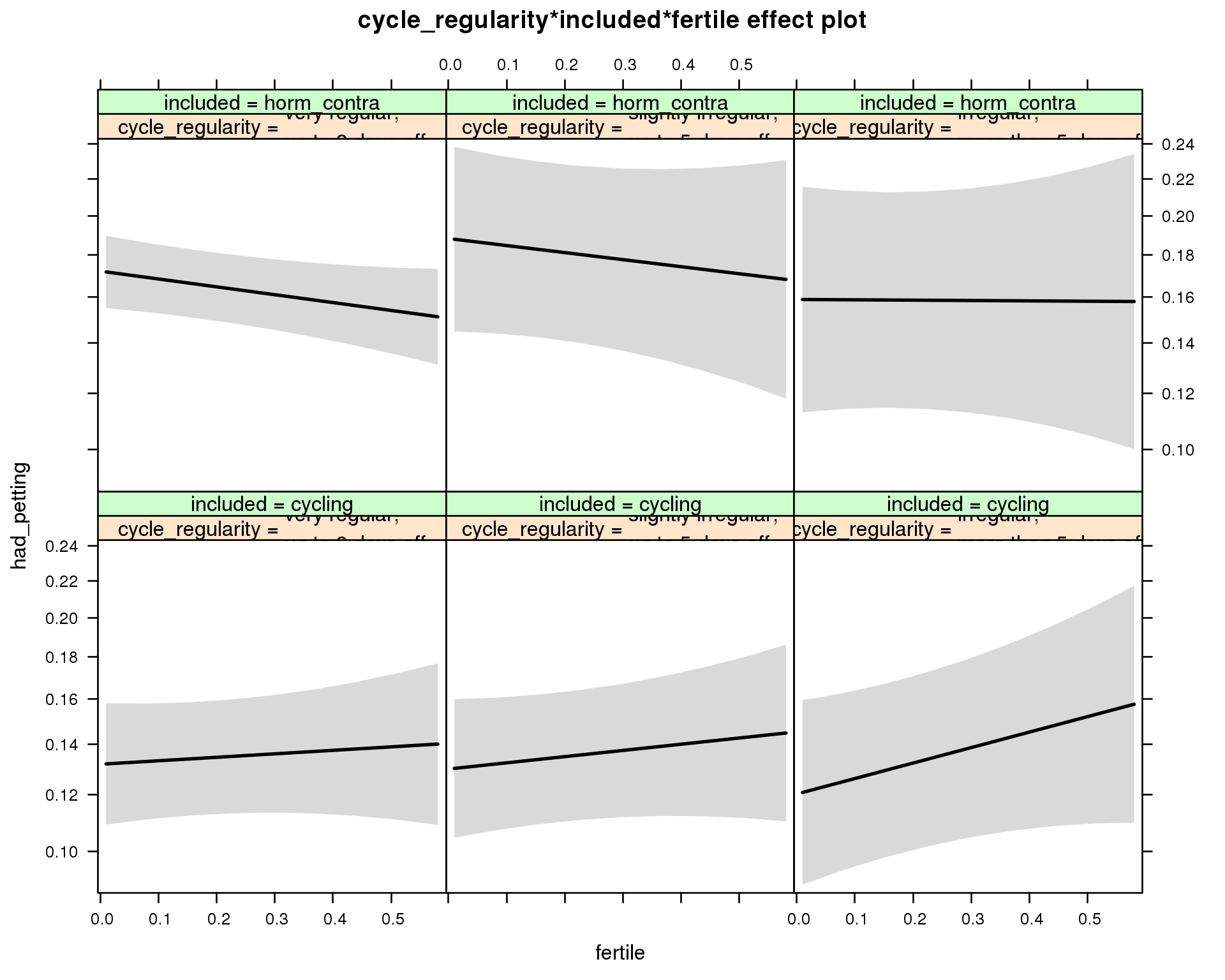
Generalized linear mixed model fit by maximum likelihood (Laplace Approximation) ['glmerMod']
Family: binomial ( probit )
Formula: had_petting ~ menstruation + fertile_mean + (1 | person) + cycle_regularity +
included + fertile + menstruation:included + cycle_regularity:included +
cycle_regularity:fertile + included:fertile + cycle_regularity:included:fertile
Data: diary
AIC BIC logLik deviance df.resid
24098 24246 -12031 24062 26685
Scaled residuals:
Min 1Q Median 3Q Max
-2.297 -0.499 -0.348 -0.177 5.395
Random effects:
Groups Name Variance Std.Dev.
person (Intercept) 0.368 0.606
Number of obs: 26703, groups: person, 1054
Fixed effects:
Estimate Std. Error z value
(Intercept) -1.07193 0.08159 -13.14
menstruationpre -0.06409 0.04922 -1.30
menstruationyes -0.12228 0.04664 -2.62
fertile_mean -0.07394 0.32482 -0.23
cycle_regularityslightly irregular,\nup to 5 days off -0.00900 0.08784 -0.10
cycle_regularityirregular,\nmore than 5 days off -0.05600 0.10566 -0.53
includedhorm_contra 0.17662 0.07294 2.42
fertile 0.06552 0.13765 0.48
menstruationpre:includedhorm_contra 0.00718 0.06170 0.12
menstruationyes:includedhorm_contra -0.03356 0.05989 -0.56
cycle_regularityslightly irregular,\nup to 5 days off:includedhorm_contra 0.07041 0.12976 0.54
cycle_regularityirregular,\nmore than 5 days off:includedhorm_contra 0.00267 0.15557 0.02
cycle_regularityslightly irregular,\nup to 5 days off:fertile 0.05139 0.18649 0.28
cycle_regularityirregular,\nmore than 5 days off:fertile 0.22594 0.22714 0.99
includedhorm_contra:fertile -0.21357 0.15858 -1.35
cycle_regularityslightly irregular,\nup to 5 days off:includedhorm_contra:fertile -0.03604 0.27108 -0.13
cycle_regularityirregular,\nmore than 5 days off:includedhorm_contra:fertile -0.08448 0.33020 -0.26
Pr(>|z|)
(Intercept) <2e-16 ***
menstruationpre 0.1928
menstruationyes 0.0087 **
fertile_mean 0.8199
cycle_regularityslightly irregular,\nup to 5 days off 0.9184
cycle_regularityirregular,\nmore than 5 days off 0.5961
includedhorm_contra 0.0155 *
fertile 0.6341
menstruationpre:includedhorm_contra 0.9074
menstruationyes:includedhorm_contra 0.5752
cycle_regularityslightly irregular,\nup to 5 days off:includedhorm_contra 0.5874
cycle_regularityirregular,\nmore than 5 days off:includedhorm_contra 0.9863
cycle_regularityslightly irregular,\nup to 5 days off:fertile 0.7829
cycle_regularityirregular,\nmore than 5 days off:fertile 0.3199
includedhorm_contra:fertile 0.1780
cycle_regularityslightly irregular,\nup to 5 days off:includedhorm_contra:fertile 0.8942
cycle_regularityirregular,\nmore than 5 days off:includedhorm_contra:fertile 0.7981
---
Signif. codes: 0 '***' 0.001 '**' 0.01 '*' 0.05 '.' 0.1 ' ' 1
convergence code: 0
Model failed to converge with max|grad| = 0.0113852 (tol = 0.001, component 1)
M_m9: Moderation by cohabitation status
model %>%
test_moderator("cohabitation", diary)| Df | AIC | BIC | logLik | deviance | Chisq | Chi Df | Pr(>Chisq) | |
|---|---|---|---|---|---|---|---|---|
| with_main | 14 | 24047 | 24161 | -12009 | 24019 | NA | NA | NA |
| with_mod | 18 | 24054 | 24202 | -12009 | 24018 | 0.5849 | 4 | 0.9647 |
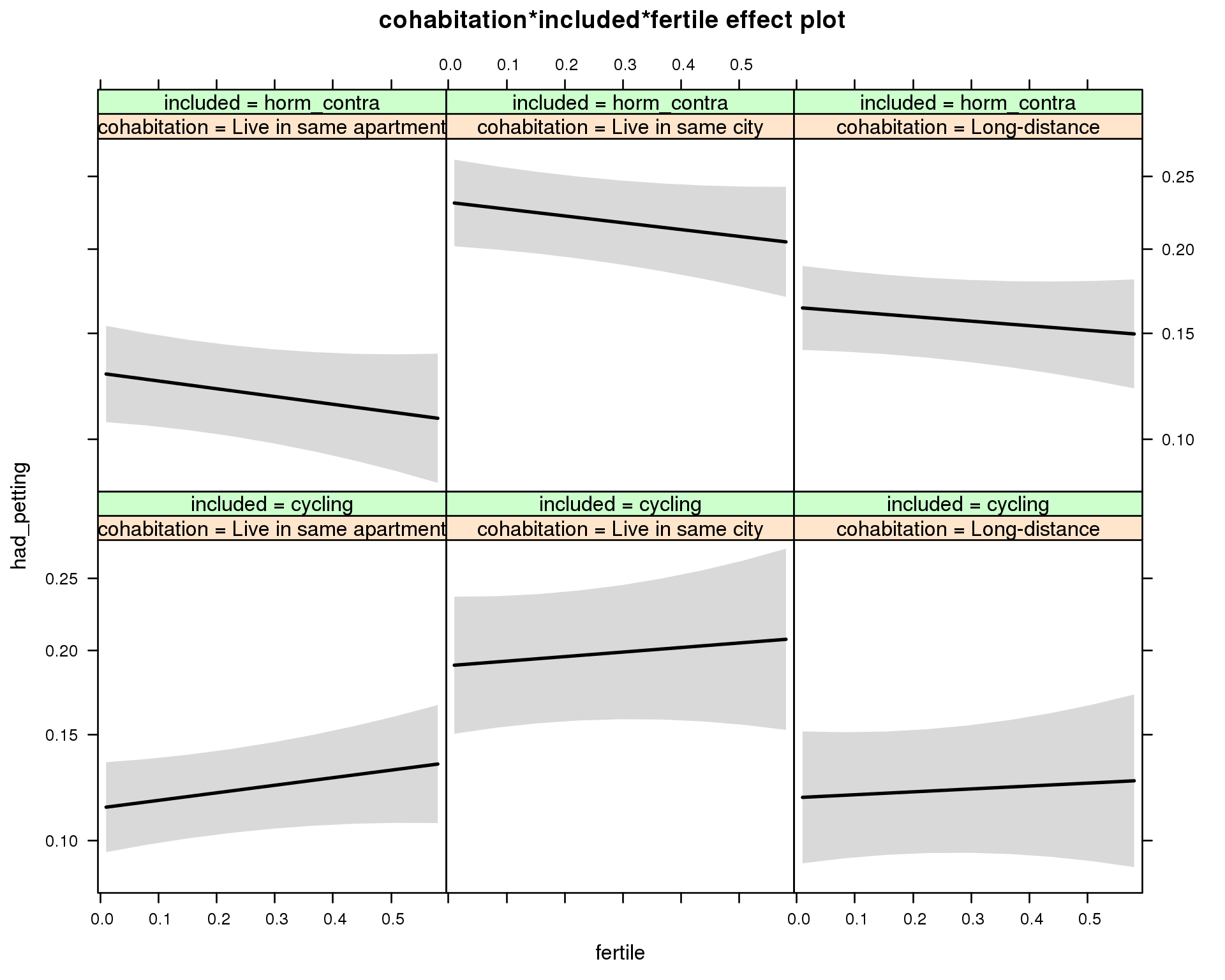
Generalized linear mixed model fit by maximum likelihood (Laplace Approximation) ['glmerMod']
Family: binomial ( probit )
Formula: had_petting ~ menstruation + fertile_mean + (1 | person) + cohabitation +
included + fertile + menstruation:included + cohabitation:included +
cohabitation:fertile + included:fertile + cohabitation:included:fertile
Data: diary
AIC BIC logLik deviance df.resid
24054 24202 -12009 24018 26685
Scaled residuals:
Min 1Q Median 3Q Max
-2.189 -0.498 -0.348 -0.174 5.243
Random effects:
Groups Name Variance Std.Dev.
person (Intercept) 0.346 0.589
Number of obs: 26703, groups: person, 1054
Fixed effects:
Estimate Std. Error z value Pr(>|z|)
(Intercept) -1.16001 0.07839 -14.80 < 2e-16 ***
menstruationpre -0.06234 0.04915 -1.27 0.20461
menstruationyes -0.11927 0.04658 -2.56 0.01045 *
fertile_mean -0.07783 0.31924 -0.24 0.80739
cohabitationLive in same city 0.32909 0.09635 3.42 0.00064 ***
cohabitationLong-distance 0.02378 0.09380 0.25 0.79987
includedhorm_contra 0.08298 0.08177 1.01 0.31022
fertile 0.17494 0.12377 1.41 0.15753
menstruationpre:includedhorm_contra 0.00123 0.06165 0.02 0.98410
menstruationyes:includedhorm_contra -0.03974 0.05982 -0.66 0.50645
cohabitationLive in same city:includedhorm_contra 0.06625 0.12312 0.54 0.59048
cohabitationLong-distance:includedhorm_contra 0.12829 0.12040 1.07 0.28666
cohabitationLive in same city:fertile -0.06984 0.20932 -0.33 0.73864
cohabitationLong-distance:fertile -0.10780 0.20544 -0.52 0.59978
includedhorm_contra:fertile -0.35464 0.18185 -1.95 0.05116 .
cohabitationLive in same city:includedhorm_contra:fertile 0.09178 0.26616 0.34 0.73022
cohabitationLong-distance:includedhorm_contra:fertile 0.18203 0.26298 0.69 0.48882
---
Signif. codes: 0 '***' 0.001 '**' 0.01 '*' 0.05 '.' 0.1 ' ' 1
convergence code: 0
Model failed to converge with max|grad| = 0.0651494 (tol = 0.001, component 1)
M_m10: Moderation by relationship status
model %>%
test_moderator("relationship_status_clean", diary)| Df | AIC | BIC | logLik | deviance | Chisq | Chi Df | Pr(>Chisq) | |
|---|---|---|---|---|---|---|---|---|
| with_main | 14 | 24051 | 24166 | -12012 | 24023 | NA | NA | NA |
| with_mod | 18 | 24055 | 24203 | -12010 | 24019 | 4.219 | 4 | 0.3772 |
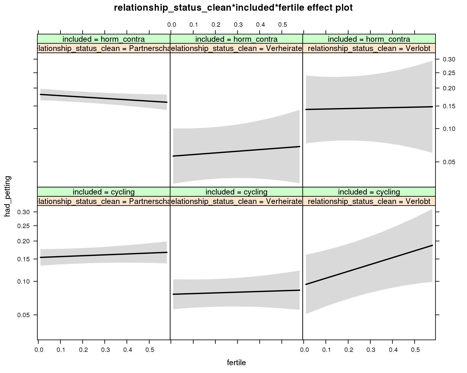
Generalized linear mixed model fit by maximum likelihood (Laplace Approximation) ['glmerMod']
Family: binomial ( probit )
Formula: had_petting ~ menstruation + fertile_mean + (1 | person) + relationship_status_clean +
included + fertile + menstruation:included + relationship_status_clean:included +
relationship_status_clean:fertile + included:fertile + relationship_status_clean:included:fertile
Data: diary
AIC BIC logLik deviance df.resid
24055 24203 -12010 24019 26685
Scaled residuals:
Min 1Q Median 3Q Max
-2.285 -0.500 -0.348 -0.178 5.284
Random effects:
Groups Name Variance Std.Dev.
person (Intercept) 0.35 0.591
Number of obs: 26703, groups: person, 1054
Fixed effects:
Estimate Std. Error z value Pr(>|z|)
(Intercept) -0.97509 0.07218 -13.51 < 2e-16 ***
menstruationpre -0.06501 0.04918 -1.32 0.1862
menstruationyes -0.12332 0.04660 -2.65 0.0081 **
fertile_mean -0.07227 0.31904 -0.23 0.8208
relationship_status_cleanVerheiratet -0.40102 0.09453 -4.24 0.000022 ***
relationship_status_cleanVerlobt -0.30031 0.17212 -1.74 0.0810 .
includedhorm_contra 0.11618 0.06148 1.89 0.0588 .
fertile 0.09640 0.10882 0.89 0.3757
menstruationpre:includedhorm_contra 0.00777 0.06166 0.13 0.8998
menstruationyes:includedhorm_contra -0.03180 0.05984 -0.53 0.5951
relationship_status_cleanVerheiratet:includedhorm_contra -0.27352 0.18448 -1.48 0.1382
relationship_status_cleanVerlobt:includedhorm_contra 0.13491 0.25823 0.52 0.6014
relationship_status_cleanVerheiratet:fertile -0.01926 0.21274 -0.09 0.9278
relationship_status_cleanVerlobt:fertile 0.64958 0.35887 1.81 0.0703 .
includedhorm_contra:fertile -0.24508 0.13133 -1.87 0.0620 .
relationship_status_cleanVerheiratet:includedhorm_contra:fertile 0.34939 0.42388 0.82 0.4098
relationship_status_cleanVerlobt:includedhorm_contra:fertile -0.44956 0.57880 -0.78 0.4373
---
Signif. codes: 0 '***' 0.001 '**' 0.01 '*' 0.05 '.' 0.1 ' ' 1
convergence code: 0
Model failed to converge with max|grad| = 0.0943412 (tol = 0.001, component 1)
Sexual intercourse
model_summaries$had_sexual_intercourseModel summary
Model summary
model %>%
print_summary()Generalized linear mixed model fit by maximum likelihood (Laplace Approximation) ['glmerMod']
Family: binomial ( probit )
Formula: had_sexual_intercourse ~ included * (menstruation + fertile) + fertile_mean + (1 | person)
Data: diary
AIC BIC logLik deviance df.resid
25698 25780 -12839 25678 26694
Scaled residuals:
Min 1Q Median 3Q Max
-2.621 -0.546 -0.375 -0.188 6.343
Random effects:
Groups Name Variance Std.Dev.
person (Intercept) 0.311 0.557
Number of obs: 26704, groups: person, 1054
Fixed effects:
Estimate Std. Error z value Pr(>|z|)
(Intercept) -1.0249 0.0650 -15.76 < 2e-16 ***
includedhorm_contra 0.2728 0.0533 5.12 0.00000031 ***
menstruationpre -0.0228 0.0470 -0.49 0.62684
menstruationyes -0.4122 0.0478 -8.62 < 2e-16 ***
fertile 0.0912 0.0946 0.96 0.33515
fertile_mean 0.4010 0.2994 1.34 0.18049
includedhorm_contra:menstruationpre -0.0682 0.0587 -1.16 0.24583
includedhorm_contra:menstruationyes -0.2119 0.0622 -3.41 0.00066 ***
includedhorm_contra:fertile -0.3197 0.1170 -2.73 0.00630 **
---
Signif. codes: 0 '***' 0.001 '**' 0.01 '*' 0.05 '.' 0.1 ' ' 1
Correlation of Fixed Effects:
(Intr) incld_ mnstrtnp mnstrtny fertil frtl_m inclddhrm_cntr:mnstrtnp
inclddhrm_c -0.492
menstrutnpr -0.287 0.354
menstrutnys -0.244 0.303 0.356
fertile -0.277 0.437 0.469 0.354
fertile_men -0.756 -0.037 -0.005 -0.004 -0.104
inclddhrm_cntr:mnstrtnp 0.238 -0.432 -0.800 -0.285 -0.374 -0.008
inclddhrm_cntr:mnstrtny 0.197 -0.360 -0.274 -0.768 -0.272 -0.006 0.338
inclddhrm_cntr:f 0.276 -0.538 -0.379 -0.286 -0.801 0.016 0.467
inclddhrm_cntr:mnstrtny
inclddhrm_c
menstrutnpr
menstrutnys
fertile
fertile_men
inclddhrm_cntr:mnstrtnp
inclddhrm_cntr:mnstrtny
inclddhrm_cntr:f 0.344
convergence code: 0
Model failed to converge with max|grad| = 0.0104007 (tol = 0.001, component 1)
Effect size standardised by residual variance (\(\frac{b}{ SD_{residual} }\)): 0.09 [-0.09;0.28].
Marginal effect plots
model %>%
plot_all_effects()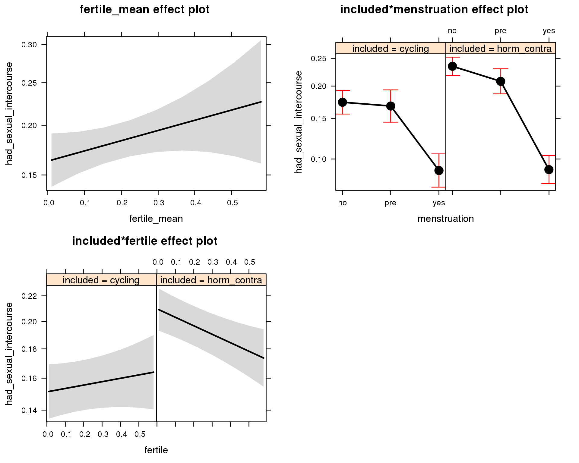
Outcome distribution
model %>%
plot_outcome(diary) + xlab(outcome_label)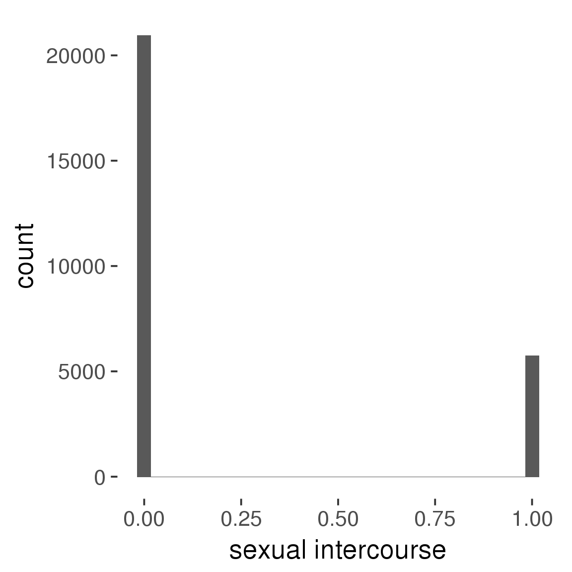
Diagnostics
model %>%
print_diagnostics()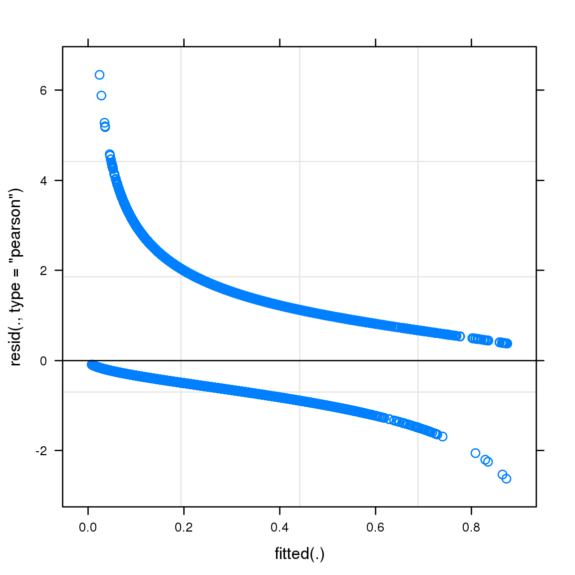
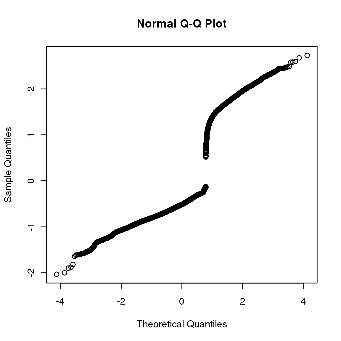
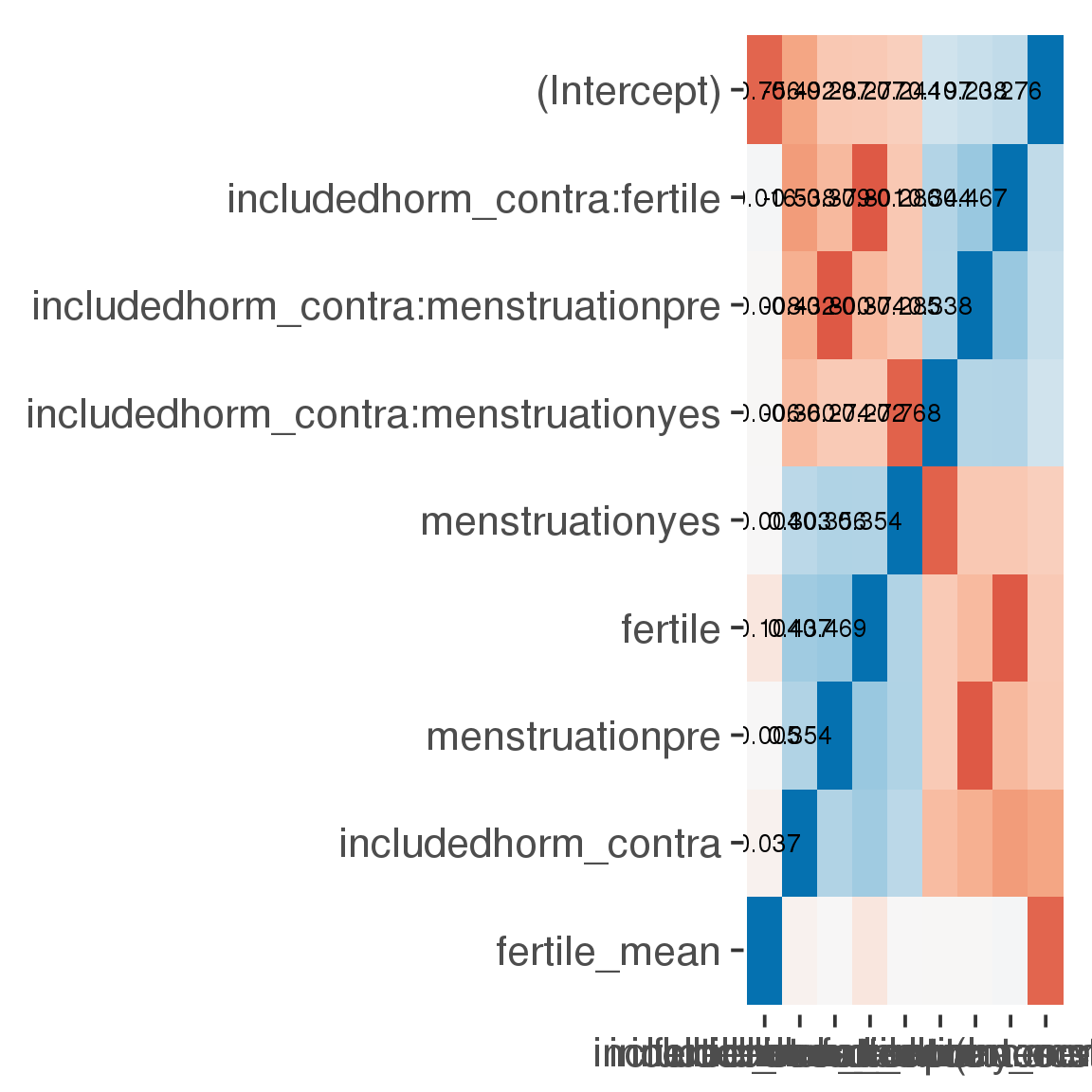
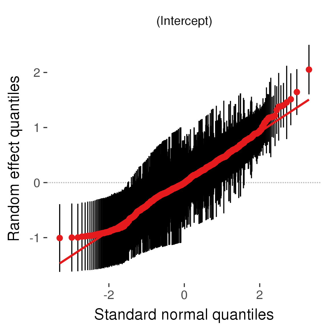
Curves
Here, we continuously plot the outcome over the course of the cycle. Because cycle lengths vary, we subset the data to cycles in a certain range. If the red curve traces the pink curve, our predictor accurately maps the relationship between fertile window probability and the outcome.
Cycle lengths from 21 to 36
Backward-counted
model %>%
plot_curve(diary %>% filter(minimum_cycle_length_diary <= 36, minimum_cycle_length_diary > 20) %>% mutate(fertile=prc_stirn_b))outcome = names(model@frame)[1]
outcome_label = recode(str_replace_all(str_replace_all(str_replace_all(outcome, "_", " "), " pair", "-pair"), " 1", ""),
"desirability 1" = "self-perceived desirability",
"NARQ admiration" = "narcissistic admiration",
"NARQ rivalry" = "narcissistic rivalry",
"extra-pair" = "extra-pair desire & behaviour",
"had sexual intercourse" = "sexual intercourse")
library(ggplot2)
# form a subset and run the model without the hormonal contraception and the fertility predictors
tmp = diary %>%
filter(!is.na(fertile), !is.na(included),
RCD > -1 * minimum_cycle_length_diary, RCD > -40)
new_form = update.formula(formula(model), new = . ~ . - fertile * included)
tmp$residuals = residuals(update(model, new_form, data = tmp , na.action = na.exclude))
tmp = tmp %>%
filter(!is.na(RCD), !is.na(residuals))
rcd_min = min(tmp$RCD)
tmp$real = FALSE
tmp_before = tmp
tmp_before$RCD = tmp_before$RCD + min(tmp$RCD) - 1
tmp_after = tmp
tmp_after$RCD = tmp_after$RCD - min(tmp$RCD) + 1
tmp$real = TRUE
tmp = bind_rows(tmp_before %>% filter(RCD > rcd_min - 11), tmp, tmp_after %>% filter(RCD < 11))GAM smooth on residuals
Here, we partialled out menstruation and individual random effects, then superimposed estimated probability of being in the fertile window scaled to the range of the estimated means. To address the periodicity of the cycle, we prepended and appended ten days of the timeseries to the end and the beginning of the timeseries. We then estimated the GAM and cut off the appended subsets before plotting.
tryCatch({
trend_plot = ggplot(tmp,aes(x = RCD, y = residuals, colour = included)) +
stat_smooth(geom = 'smooth',size = 0.8, fill = "#9ECAE1", method = 'gam', formula = y ~ s(x))
}, error = function(e){cat_message(e, "danger")})
tryCatch({
trend_data = ggplot_build(trend_plot)$data[[1]]
}, error = function(e){cat_message(e, "danger")})
trend_data$RCD = round(trend_data$x)
trend_data = left_join(trend_data, tmp %>% select(real, RCD,fertile) %>% unique(), by = "RCD")
trend_data %>%
filter(real == TRUE) %>%
mutate(superimposed = ( ( (fertile - 0.01)/0.58) * (max(y)-min(y) ) ) + min(y) ) ->
trend_data
ggplot(trend_data) +
geom_ribbon(aes(x = x, ymin = ymin, ymax = ymax, fill = factor(group)), alpha = 0.2) +
geom_line(aes(x = x, y = y, colour = factor(group)), size = 0.8, stat = "identity") +
scale_x_continuous(caption_x) +
geom_line(aes(x = x, y = superimposed), color = "#a83fbf", size = 1, linetype = 'dashed') +
annotate("text",x = mean(trend_data$x), y = max(trend_data$superimposed,na.rm=T) + 0.1, label = 'superimposed fertility peak', color = "#a83fbf") +
scale_y_continuous(outcome_label) +
ggtitle("GAM smooth, residuals") +
scale_color_manual("Contraception status",values = c("2"="black","1"= "red"), labels = c("2"="hormonally\ncontracepting","1"="cycling"), guide = F) +
scale_fill_manual("Contraception status",values = c("2"="black","1"= "red"), labels = c("2"="hormonally\ncontracepting","1"="cycling"), guide = F)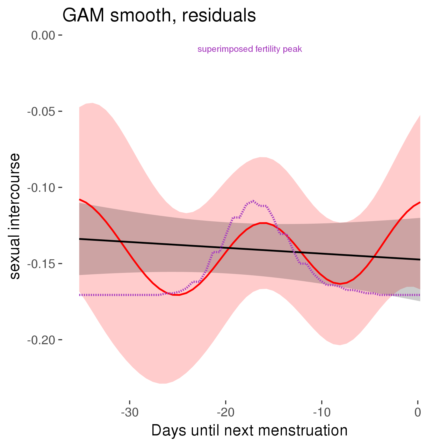
GAM smooth on raw data
As before, but without partialling anything out.
tryCatch({
trend_plot = ggplot(tmp,aes_string(x = "RCD", y = outcome, colour = "included")) +
stat_smooth(geom = 'smooth',size = 0.8, fill = "#9ECAE1", method = 'gam', formula = y ~ s(x))
}, error = function(e){cat_message(e, "danger")})
tryCatch({
trend_data = ggplot_build(trend_plot)$data[[1]]
}, error = function(e){cat_message(e, "danger")})
trend_data$RCD = round(trend_data$x)
trend_data = left_join(trend_data, tmp %>% select(real, RCD,fertile) %>% unique(), by = "RCD")
trend_data %>%
filter(real == TRUE) %>%
mutate(superimposed = ( ( (fertile - 0.01)/0.58) * (max(y)-min(y) ) ) + min(y) ) ->
trend_data
plot1b = ggplot(trend_data) +
geom_ribbon(aes(x = x, ymin = ymin, ymax = ymax, fill = factor(group)), alpha = 0.2) +
geom_line(aes(x = x, y = y, colour = factor(group)), size = 0.8, stat = "identity") +
scale_x_continuous(caption_x) +
geom_line(aes(x = x, y = superimposed), color = "#a83fbf", size = 1, linetype = 'dashed') +
annotate("text",x = mean(trend_data$x), y = max(trend_data$superimposed,na.rm=T) + 0.1, label = 'superimposed fertility peak', color = "#a83fbf") +
scale_y_continuous(outcome_label) +
ggtitle("GAM smooth, raw data") +
scale_color_manual("Contraception status",values = c("2"="black","1"= "red"), labels = c("2"="hormonally\ncontracepting","1"="cycling"), guide = F) +
scale_fill_manual("Contraception status",values = c("2"="black","1"= "red"), labels = c("2"="hormonally\ncontracepting","1"="cycling"), guide = F)
suppressWarnings(print(plot1b))
Means and standard errors over raw data
Nothing partialled out, just straight means with bootstrapped confidence intervals.
tryCatch({
trend_plot = ggplot(tmp,aes_string(x = "RCD", y = outcome, colour = "included")) +
geom_pointrange(size = 0.8, stat = 'summary', fun.data = "mean_cl_boot")
}, error = function(e){cat_message(e, "danger")})
tryCatch({
trend_data = ggplot_build(trend_plot)$data[[1]]
}, error = function(e){cat_message(e, "danger")})
trend_data$RCD = round(trend_data$x)
trend_data = left_join(trend_data, tmp %>% select(real, RCD,fertile) %>% unique(), by = "RCD")
trend_data %>%
filter(real == TRUE) %>%
mutate(superimposed = ( ( (fertile - 0.01)/0.58) * (max(y)-min(y) ) ) + min(y) ) ->
trend_data
plot3 = ggplot(trend_data) +
geom_pointrange(aes(x = x, y = y, ymin = ymin,ymax = ymax, colour = factor(group)), size = 0.8, stat = "identity", alpha = 0.6, position = position_dodge(width = .5)) +
scale_x_continuous("Days until next menstruation") +
geom_line(aes(x= x, y = superimposed), color = "#a83fbf", size = 1, linetype = 'dashed') +
annotate("text",x = mean(trend_data$x), y = max(trend_data$superimposed,na.rm=T) + 0.1, label = 'superimposed fertility peak', color = "#a83fbf") +
scale_y_continuous(outcome_label) +
ggtitle("Means with standard errors, raw data") +
scale_color_manual("Contraception status",values = c("2"="black","1"= "red"), labels = c("2"="hormonally\ncontracepting","1"="cycling"), guide = F) +
scale_fill_manual("Contraception status",values = c("2"="black","1"= "red"), labels = c("2"="hormonally\ncontracepting","1"="cycling"), guide = F)
suppressWarnings(print(plot3))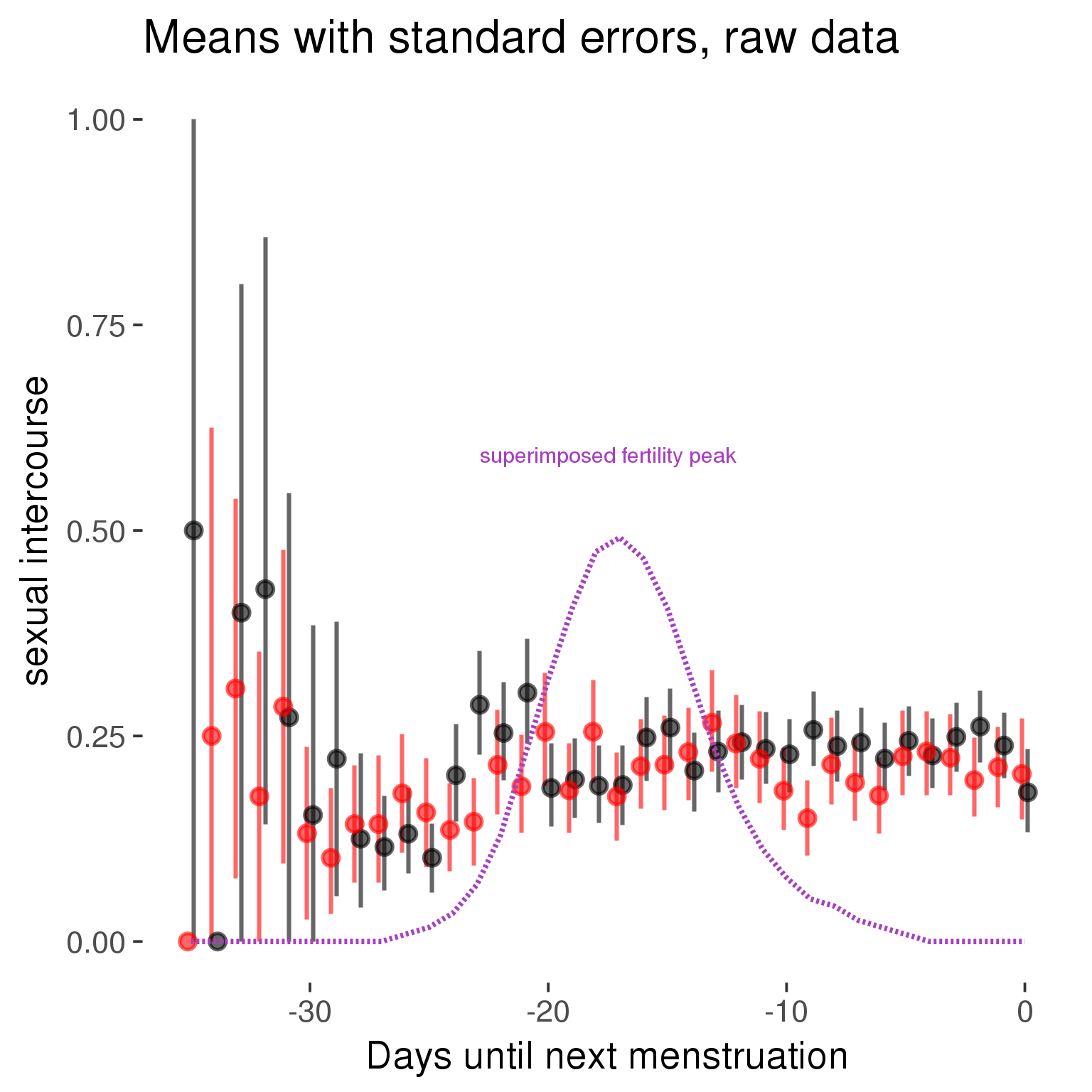
Forward-counted
model %>%
plot_curve(diary %>% filter(minimum_cycle_length_diary <= 36, minimum_cycle_length_diary > 20) %>% mutate(RCD = FCD, fertile = prc_stirn_b_forward_counted), caption_x = "Days since last menstruation")outcome = names(model@frame)[1]
outcome_label = recode(str_replace_all(str_replace_all(str_replace_all(outcome, "_", " "), " pair", "-pair"), " 1", ""),
"desirability 1" = "self-perceived desirability",
"NARQ admiration" = "narcissistic admiration",
"NARQ rivalry" = "narcissistic rivalry",
"extra-pair" = "extra-pair desire & behaviour",
"had sexual intercourse" = "sexual intercourse")
library(ggplot2)
# form a subset and run the model without the hormonal contraception and the fertility predictors
tmp = diary %>%
filter(!is.na(fertile), !is.na(included),
RCD > -1 * minimum_cycle_length_diary, RCD > -40)
new_form = update.formula(formula(model), new = . ~ . - fertile * included)
tmp$residuals = residuals(update(model, new_form, data = tmp , na.action = na.exclude))
tmp = tmp %>%
filter(!is.na(RCD), !is.na(residuals))
rcd_min = min(tmp$RCD)
tmp$real = FALSE
tmp_before = tmp
tmp_before$RCD = tmp_before$RCD + min(tmp$RCD) - 1
tmp_after = tmp
tmp_after$RCD = tmp_after$RCD - min(tmp$RCD) + 1
tmp$real = TRUE
tmp = bind_rows(tmp_before %>% filter(RCD > rcd_min - 11), tmp, tmp_after %>% filter(RCD < 11))GAM smooth on residuals
Here, we partialled out menstruation and individual random effects, then superimposed estimated probability of being in the fertile window scaled to the range of the estimated means. To address the periodicity of the cycle, we prepended and appended ten days of the timeseries to the end and the beginning of the timeseries. We then estimated the GAM and cut off the appended subsets before plotting.
tryCatch({
trend_plot = ggplot(tmp,aes(x = RCD, y = residuals, colour = included)) +
stat_smooth(geom = 'smooth',size = 0.8, fill = "#9ECAE1", method = 'gam', formula = y ~ s(x))
}, error = function(e){cat_message(e, "danger")})
tryCatch({
trend_data = ggplot_build(trend_plot)$data[[1]]
}, error = function(e){cat_message(e, "danger")})
trend_data$RCD = round(trend_data$x)
trend_data = left_join(trend_data, tmp %>% select(real, RCD,fertile) %>% unique(), by = "RCD")
trend_data %>%
filter(real == TRUE) %>%
mutate(superimposed = ( ( (fertile - 0.01)/0.58) * (max(y)-min(y) ) ) + min(y) ) ->
trend_data
ggplot(trend_data) +
geom_ribbon(aes(x = x, ymin = ymin, ymax = ymax, fill = factor(group)), alpha = 0.2) +
geom_line(aes(x = x, y = y, colour = factor(group)), size = 0.8, stat = "identity") +
scale_x_continuous(caption_x) +
geom_line(aes(x = x, y = superimposed), color = "#a83fbf", size = 1, linetype = 'dashed') +
annotate("text",x = mean(trend_data$x), y = max(trend_data$superimposed,na.rm=T) + 0.1, label = 'superimposed fertility peak', color = "#a83fbf") +
scale_y_continuous(outcome_label) +
ggtitle("GAM smooth, residuals") +
scale_color_manual("Contraception status",values = c("2"="black","1"= "red"), labels = c("2"="hormonally\ncontracepting","1"="cycling"), guide = F) +
scale_fill_manual("Contraception status",values = c("2"="black","1"= "red"), labels = c("2"="hormonally\ncontracepting","1"="cycling"), guide = F)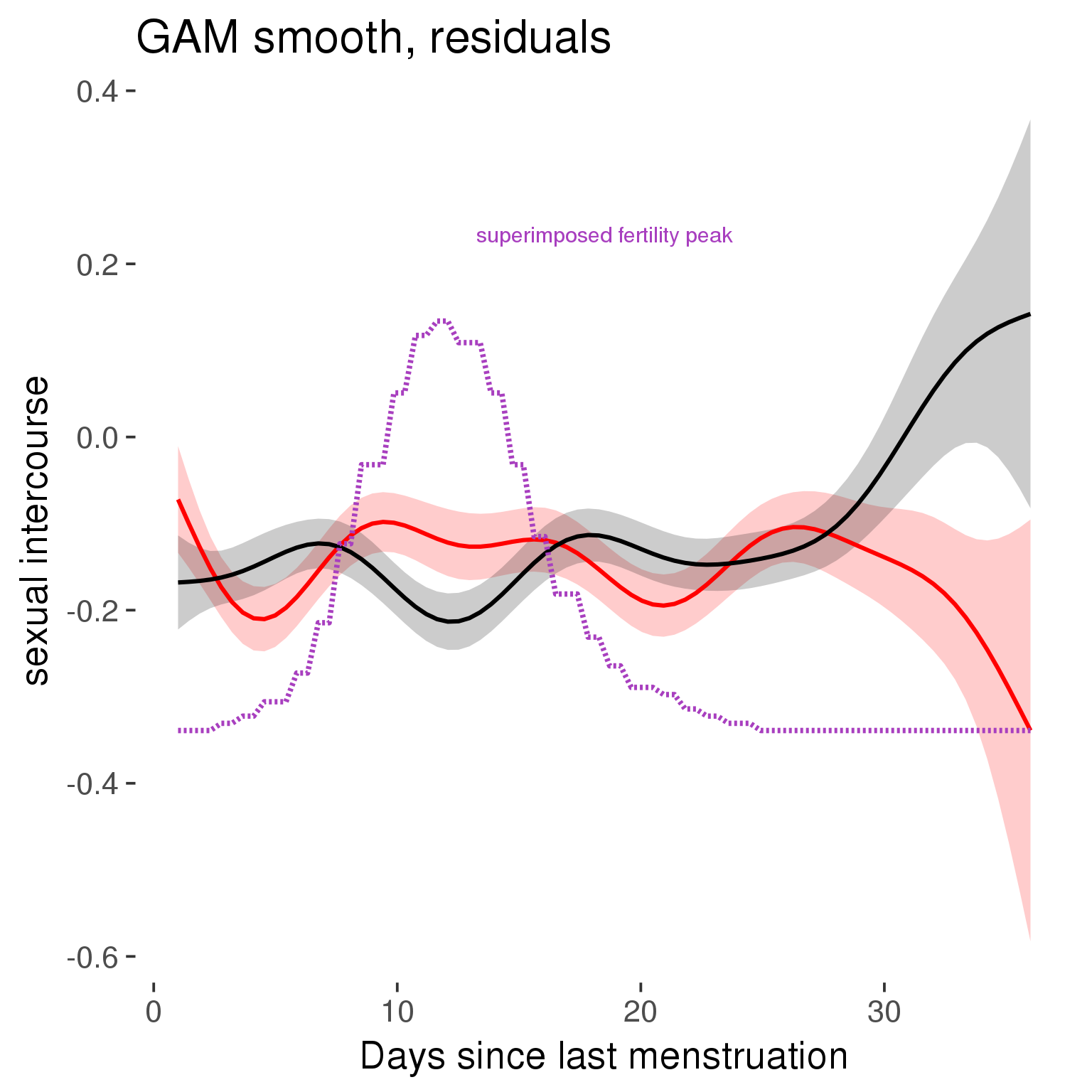
GAM smooth on raw data
As before, but without partialling anything out.
tryCatch({
trend_plot = ggplot(tmp,aes_string(x = "RCD", y = outcome, colour = "included")) +
stat_smooth(geom = 'smooth',size = 0.8, fill = "#9ECAE1", method = 'gam', formula = y ~ s(x))
}, error = function(e){cat_message(e, "danger")})
tryCatch({
trend_data = ggplot_build(trend_plot)$data[[1]]
}, error = function(e){cat_message(e, "danger")})
trend_data$RCD = round(trend_data$x)
trend_data = left_join(trend_data, tmp %>% select(real, RCD,fertile) %>% unique(), by = "RCD")
trend_data %>%
filter(real == TRUE) %>%
mutate(superimposed = ( ( (fertile - 0.01)/0.58) * (max(y)-min(y) ) ) + min(y) ) ->
trend_data
plot1b = ggplot(trend_data) +
geom_ribbon(aes(x = x, ymin = ymin, ymax = ymax, fill = factor(group)), alpha = 0.2) +
geom_line(aes(x = x, y = y, colour = factor(group)), size = 0.8, stat = "identity") +
scale_x_continuous(caption_x) +
geom_line(aes(x = x, y = superimposed), color = "#a83fbf", size = 1, linetype = 'dashed') +
annotate("text",x = mean(trend_data$x), y = max(trend_data$superimposed,na.rm=T) + 0.1, label = 'superimposed fertility peak', color = "#a83fbf") +
scale_y_continuous(outcome_label) +
ggtitle("GAM smooth, raw data") +
scale_color_manual("Contraception status",values = c("2"="black","1"= "red"), labels = c("2"="hormonally\ncontracepting","1"="cycling"), guide = F) +
scale_fill_manual("Contraception status",values = c("2"="black","1"= "red"), labels = c("2"="hormonally\ncontracepting","1"="cycling"), guide = F)
suppressWarnings(print(plot1b))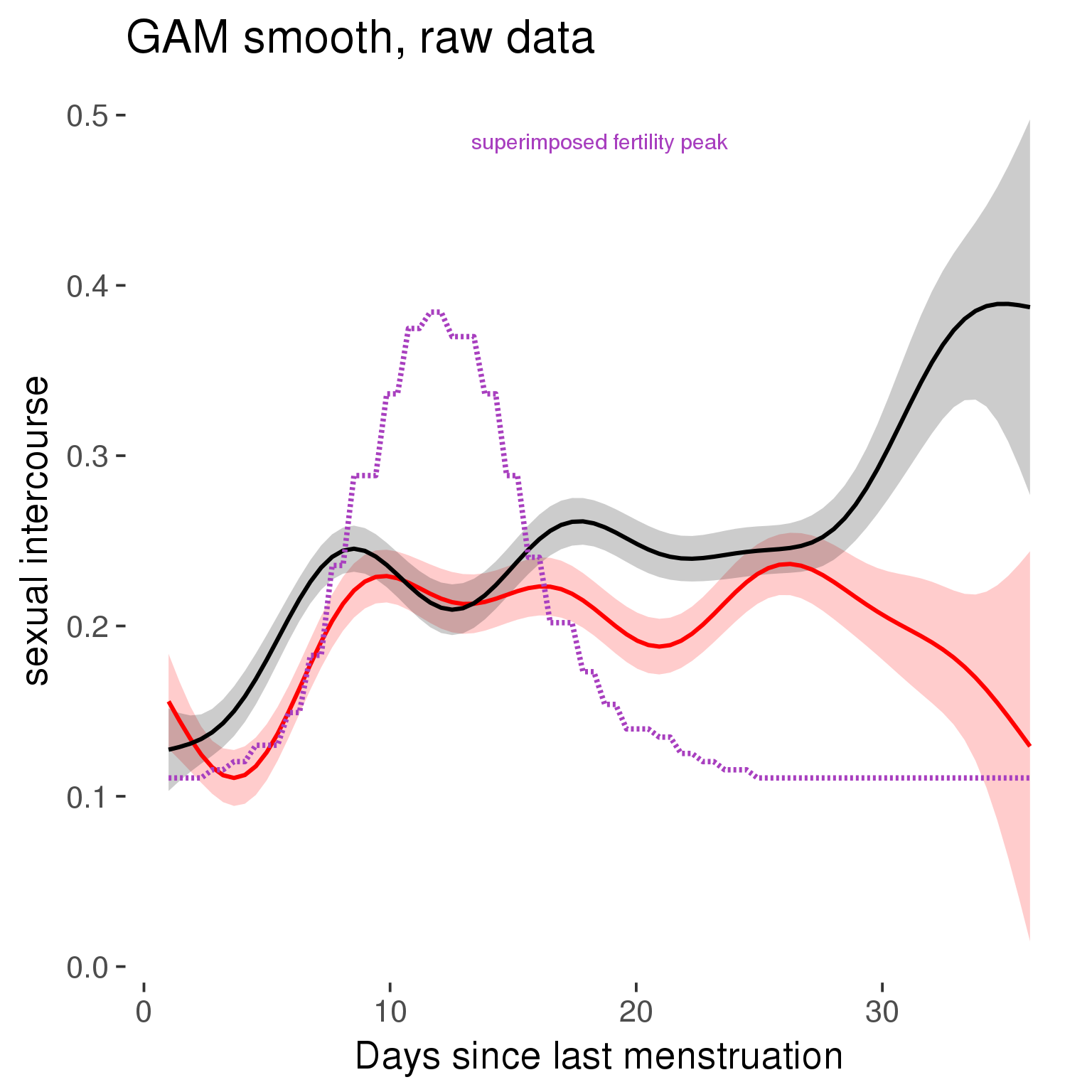
Means and standard errors over raw data
Nothing partialled out, just straight means with bootstrapped confidence intervals.
tryCatch({
trend_plot = ggplot(tmp,aes_string(x = "RCD", y = outcome, colour = "included")) +
geom_pointrange(size = 0.8, stat = 'summary', fun.data = "mean_cl_boot")
}, error = function(e){cat_message(e, "danger")})
tryCatch({
trend_data = ggplot_build(trend_plot)$data[[1]]
}, error = function(e){cat_message(e, "danger")})
trend_data$RCD = round(trend_data$x)
trend_data = left_join(trend_data, tmp %>% select(real, RCD,fertile) %>% unique(), by = "RCD")
trend_data %>%
filter(real == TRUE) %>%
mutate(superimposed = ( ( (fertile - 0.01)/0.58) * (max(y)-min(y) ) ) + min(y) ) ->
trend_data
plot3 = ggplot(trend_data) +
geom_pointrange(aes(x = x, y = y, ymin = ymin,ymax = ymax, colour = factor(group)), size = 0.8, stat = "identity", alpha = 0.6, position = position_dodge(width = .5)) +
scale_x_continuous("Days until next menstruation") +
geom_line(aes(x= x, y = superimposed), color = "#a83fbf", size = 1, linetype = 'dashed') +
annotate("text",x = mean(trend_data$x), y = max(trend_data$superimposed,na.rm=T) + 0.1, label = 'superimposed fertility peak', color = "#a83fbf") +
scale_y_continuous(outcome_label) +
ggtitle("Means with standard errors, raw data") +
scale_color_manual("Contraception status",values = c("2"="black","1"= "red"), labels = c("2"="hormonally\ncontracepting","1"="cycling"), guide = F) +
scale_fill_manual("Contraception status",values = c("2"="black","1"= "red"), labels = c("2"="hormonally\ncontracepting","1"="cycling"), guide = F)
suppressWarnings(print(plot3))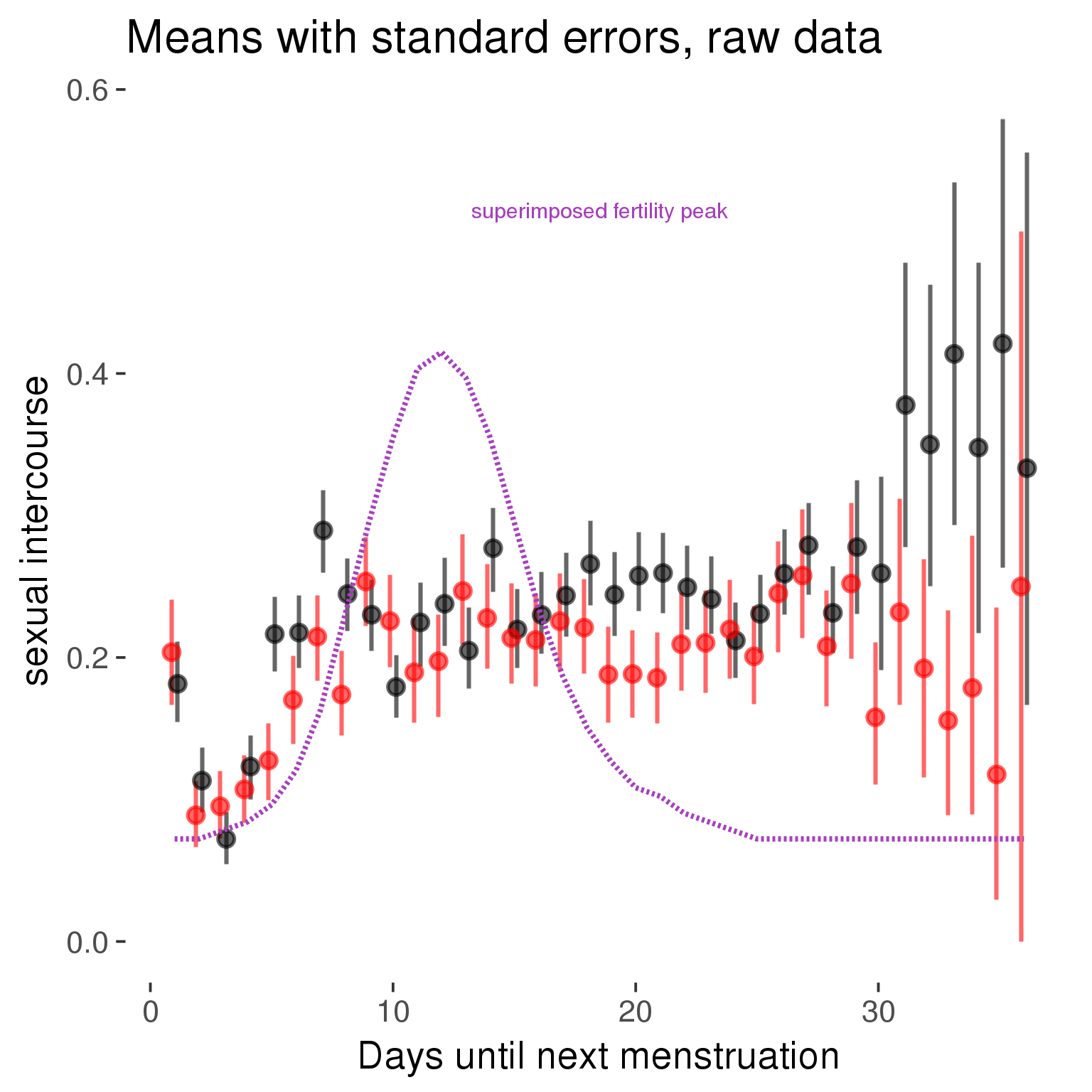
Cycle lengths from 27 to 30
Backward-counted
model %>%
plot_curve(diary %>% filter(minimum_cycle_length_diary <= 30, minimum_cycle_length_diary >= 27) %>% mutate(fertile=prc_stirn_b))outcome = names(model@frame)[1]
outcome_label = recode(str_replace_all(str_replace_all(str_replace_all(outcome, "_", " "), " pair", "-pair"), " 1", ""),
"desirability 1" = "self-perceived desirability",
"NARQ admiration" = "narcissistic admiration",
"NARQ rivalry" = "narcissistic rivalry",
"extra-pair" = "extra-pair desire & behaviour",
"had sexual intercourse" = "sexual intercourse")
library(ggplot2)
# form a subset and run the model without the hormonal contraception and the fertility predictors
tmp = diary %>%
filter(!is.na(fertile), !is.na(included),
RCD > -1 * minimum_cycle_length_diary, RCD > -40)
new_form = update.formula(formula(model), new = . ~ . - fertile * included)
tmp$residuals = residuals(update(model, new_form, data = tmp , na.action = na.exclude))
tmp = tmp %>%
filter(!is.na(RCD), !is.na(residuals))
rcd_min = min(tmp$RCD)
tmp$real = FALSE
tmp_before = tmp
tmp_before$RCD = tmp_before$RCD + min(tmp$RCD) - 1
tmp_after = tmp
tmp_after$RCD = tmp_after$RCD - min(tmp$RCD) + 1
tmp$real = TRUE
tmp = bind_rows(tmp_before %>% filter(RCD > rcd_min - 11), tmp, tmp_after %>% filter(RCD < 11))GAM smooth on residuals
Here, we partialled out menstruation and individual random effects, then superimposed estimated probability of being in the fertile window scaled to the range of the estimated means. To address the periodicity of the cycle, we prepended and appended ten days of the timeseries to the end and the beginning of the timeseries. We then estimated the GAM and cut off the appended subsets before plotting.
tryCatch({
trend_plot = ggplot(tmp,aes(x = RCD, y = residuals, colour = included)) +
stat_smooth(geom = 'smooth',size = 0.8, fill = "#9ECAE1", method = 'gam', formula = y ~ s(x))
}, error = function(e){cat_message(e, "danger")})
tryCatch({
trend_data = ggplot_build(trend_plot)$data[[1]]
}, error = function(e){cat_message(e, "danger")})
trend_data$RCD = round(trend_data$x)
trend_data = left_join(trend_data, tmp %>% select(real, RCD,fertile) %>% unique(), by = "RCD")
trend_data %>%
filter(real == TRUE) %>%
mutate(superimposed = ( ( (fertile - 0.01)/0.58) * (max(y)-min(y) ) ) + min(y) ) ->
trend_data
ggplot(trend_data) +
geom_ribbon(aes(x = x, ymin = ymin, ymax = ymax, fill = factor(group)), alpha = 0.2) +
geom_line(aes(x = x, y = y, colour = factor(group)), size = 0.8, stat = "identity") +
scale_x_continuous(caption_x) +
geom_line(aes(x = x, y = superimposed), color = "#a83fbf", size = 1, linetype = 'dashed') +
annotate("text",x = mean(trend_data$x), y = max(trend_data$superimposed,na.rm=T) + 0.1, label = 'superimposed fertility peak', color = "#a83fbf") +
scale_y_continuous(outcome_label) +
ggtitle("GAM smooth, residuals") +
scale_color_manual("Contraception status",values = c("2"="black","1"= "red"), labels = c("2"="hormonally\ncontracepting","1"="cycling"), guide = F) +
scale_fill_manual("Contraception status",values = c("2"="black","1"= "red"), labels = c("2"="hormonally\ncontracepting","1"="cycling"), guide = F)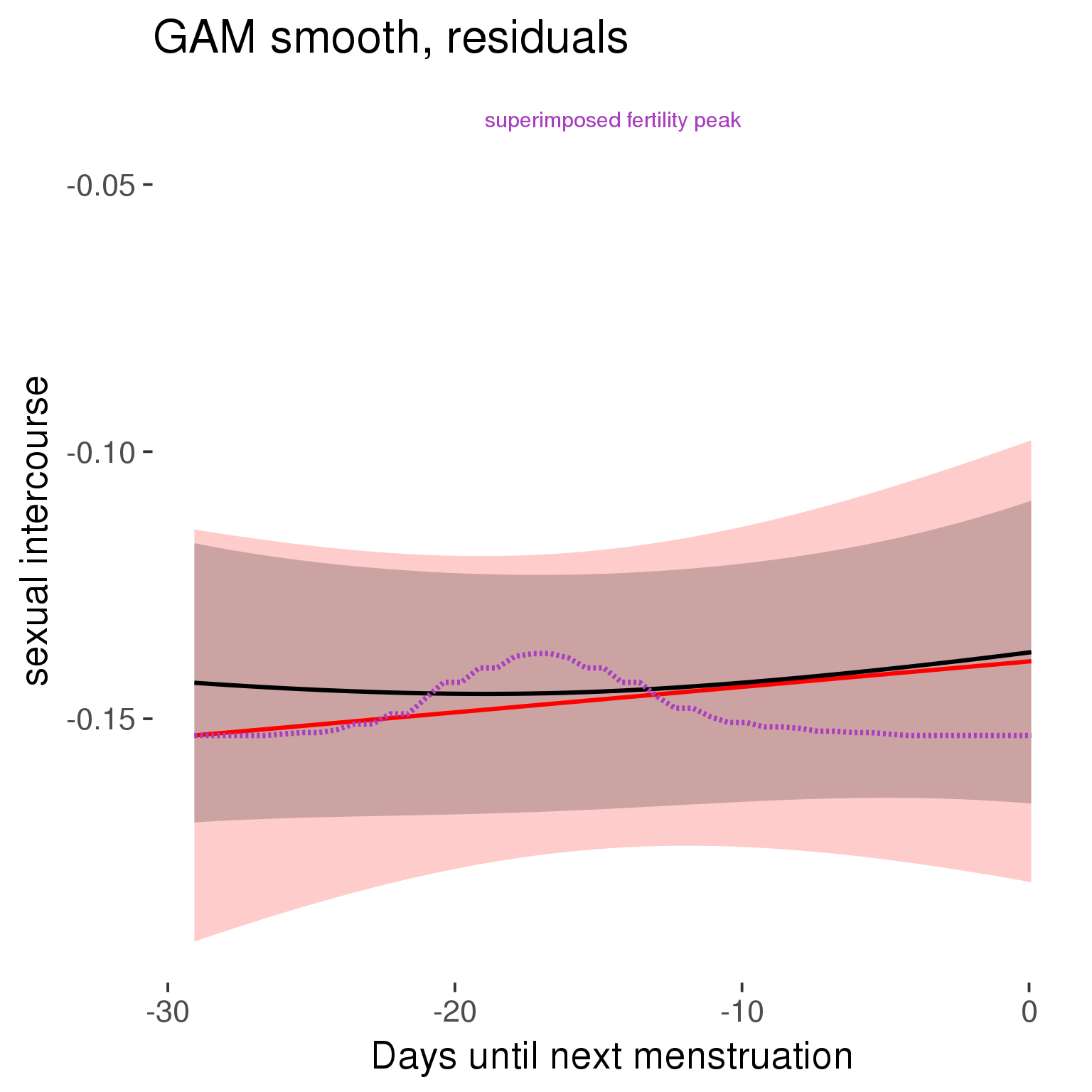
GAM smooth on raw data
As before, but without partialling anything out.
tryCatch({
trend_plot = ggplot(tmp,aes_string(x = "RCD", y = outcome, colour = "included")) +
stat_smooth(geom = 'smooth',size = 0.8, fill = "#9ECAE1", method = 'gam', formula = y ~ s(x))
}, error = function(e){cat_message(e, "danger")})
tryCatch({
trend_data = ggplot_build(trend_plot)$data[[1]]
}, error = function(e){cat_message(e, "danger")})
trend_data$RCD = round(trend_data$x)
trend_data = left_join(trend_data, tmp %>% select(real, RCD,fertile) %>% unique(), by = "RCD")
trend_data %>%
filter(real == TRUE) %>%
mutate(superimposed = ( ( (fertile - 0.01)/0.58) * (max(y)-min(y) ) ) + min(y) ) ->
trend_data
plot1b = ggplot(trend_data) +
geom_ribbon(aes(x = x, ymin = ymin, ymax = ymax, fill = factor(group)), alpha = 0.2) +
geom_line(aes(x = x, y = y, colour = factor(group)), size = 0.8, stat = "identity") +
scale_x_continuous(caption_x) +
geom_line(aes(x = x, y = superimposed), color = "#a83fbf", size = 1, linetype = 'dashed') +
annotate("text",x = mean(trend_data$x), y = max(trend_data$superimposed,na.rm=T) + 0.1, label = 'superimposed fertility peak', color = "#a83fbf") +
scale_y_continuous(outcome_label) +
ggtitle("GAM smooth, raw data") +
scale_color_manual("Contraception status",values = c("2"="black","1"= "red"), labels = c("2"="hormonally\ncontracepting","1"="cycling"), guide = F) +
scale_fill_manual("Contraception status",values = c("2"="black","1"= "red"), labels = c("2"="hormonally\ncontracepting","1"="cycling"), guide = F)
suppressWarnings(print(plot1b))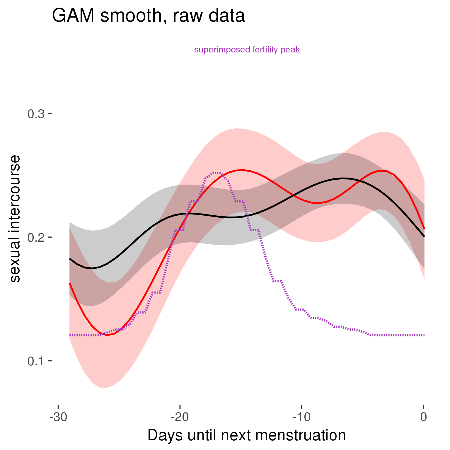
Means and standard errors over raw data
Nothing partialled out, just straight means with bootstrapped confidence intervals.
tryCatch({
trend_plot = ggplot(tmp,aes_string(x = "RCD", y = outcome, colour = "included")) +
geom_pointrange(size = 0.8, stat = 'summary', fun.data = "mean_cl_boot")
}, error = function(e){cat_message(e, "danger")})
tryCatch({
trend_data = ggplot_build(trend_plot)$data[[1]]
}, error = function(e){cat_message(e, "danger")})
trend_data$RCD = round(trend_data$x)
trend_data = left_join(trend_data, tmp %>% select(real, RCD,fertile) %>% unique(), by = "RCD")
trend_data %>%
filter(real == TRUE) %>%
mutate(superimposed = ( ( (fertile - 0.01)/0.58) * (max(y)-min(y) ) ) + min(y) ) ->
trend_data
plot3 = ggplot(trend_data) +
geom_pointrange(aes(x = x, y = y, ymin = ymin,ymax = ymax, colour = factor(group)), size = 0.8, stat = "identity", alpha = 0.6, position = position_dodge(width = .5)) +
scale_x_continuous("Days until next menstruation") +
geom_line(aes(x= x, y = superimposed), color = "#a83fbf", size = 1, linetype = 'dashed') +
annotate("text",x = mean(trend_data$x), y = max(trend_data$superimposed,na.rm=T) + 0.1, label = 'superimposed fertility peak', color = "#a83fbf") +
scale_y_continuous(outcome_label) +
ggtitle("Means with standard errors, raw data") +
scale_color_manual("Contraception status",values = c("2"="black","1"= "red"), labels = c("2"="hormonally\ncontracepting","1"="cycling"), guide = F) +
scale_fill_manual("Contraception status",values = c("2"="black","1"= "red"), labels = c("2"="hormonally\ncontracepting","1"="cycling"), guide = F)
suppressWarnings(print(plot3))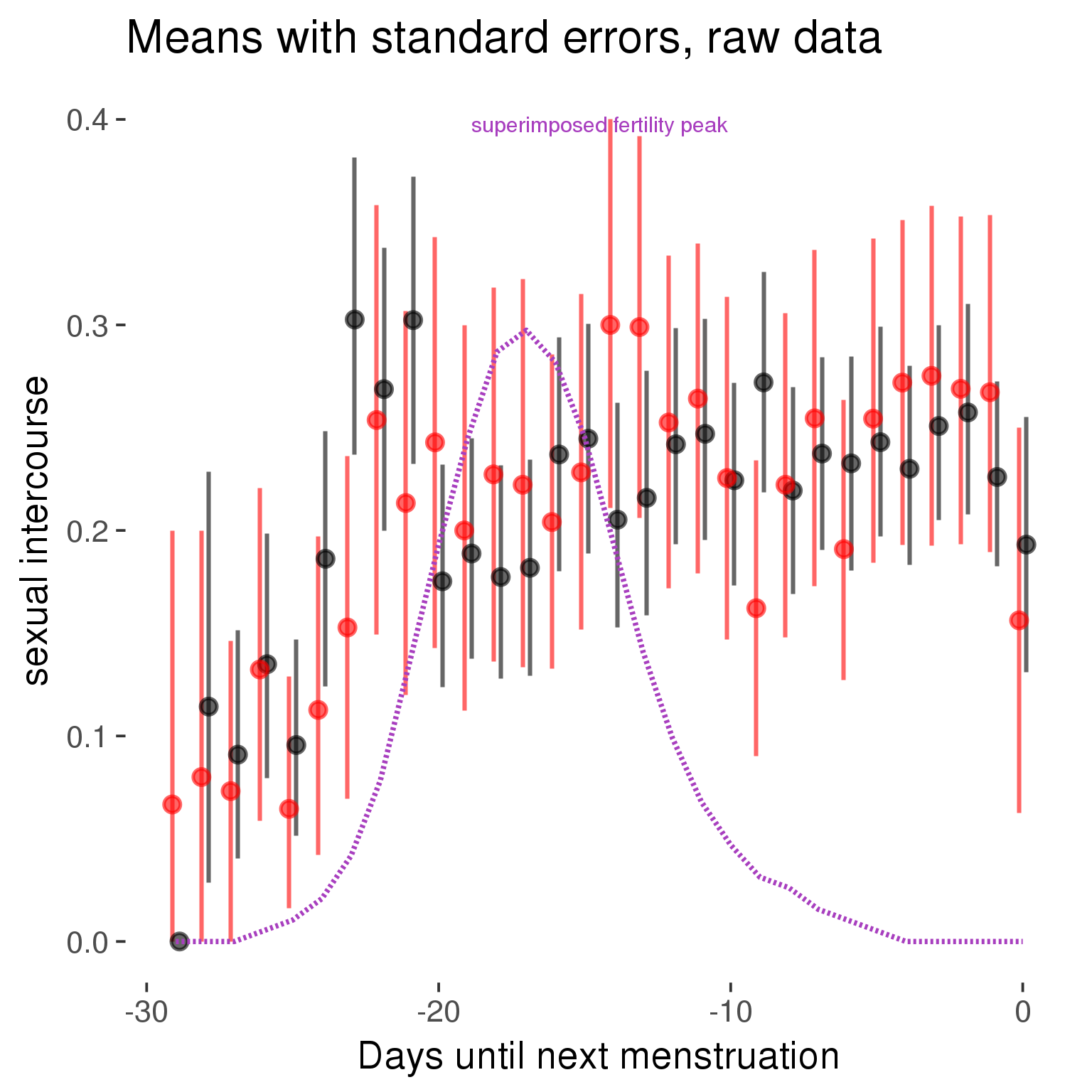
Forward-counted
model %>%
plot_curve(diary %>% filter(minimum_cycle_length_diary <= 30, minimum_cycle_length_diary >= 27) %>% mutate(RCD = FCD, fertile = prc_stirn_b_forward_counted), caption_x = "Days since last menstruation")outcome = names(model@frame)[1]
outcome_label = recode(str_replace_all(str_replace_all(str_replace_all(outcome, "_", " "), " pair", "-pair"), " 1", ""),
"desirability 1" = "self-perceived desirability",
"NARQ admiration" = "narcissistic admiration",
"NARQ rivalry" = "narcissistic rivalry",
"extra-pair" = "extra-pair desire & behaviour",
"had sexual intercourse" = "sexual intercourse")
library(ggplot2)
# form a subset and run the model without the hormonal contraception and the fertility predictors
tmp = diary %>%
filter(!is.na(fertile), !is.na(included),
RCD > -1 * minimum_cycle_length_diary, RCD > -40)
new_form = update.formula(formula(model), new = . ~ . - fertile * included)
tmp$residuals = residuals(update(model, new_form, data = tmp , na.action = na.exclude))
tmp = tmp %>%
filter(!is.na(RCD), !is.na(residuals))
rcd_min = min(tmp$RCD)
tmp$real = FALSE
tmp_before = tmp
tmp_before$RCD = tmp_before$RCD + min(tmp$RCD) - 1
tmp_after = tmp
tmp_after$RCD = tmp_after$RCD - min(tmp$RCD) + 1
tmp$real = TRUE
tmp = bind_rows(tmp_before %>% filter(RCD > rcd_min - 11), tmp, tmp_after %>% filter(RCD < 11))GAM smooth on residuals
Here, we partialled out menstruation and individual random effects, then superimposed estimated probability of being in the fertile window scaled to the range of the estimated means. To address the periodicity of the cycle, we prepended and appended ten days of the timeseries to the end and the beginning of the timeseries. We then estimated the GAM and cut off the appended subsets before plotting.
tryCatch({
trend_plot = ggplot(tmp,aes(x = RCD, y = residuals, colour = included)) +
stat_smooth(geom = 'smooth',size = 0.8, fill = "#9ECAE1", method = 'gam', formula = y ~ s(x))
}, error = function(e){cat_message(e, "danger")})
tryCatch({
trend_data = ggplot_build(trend_plot)$data[[1]]
}, error = function(e){cat_message(e, "danger")})
trend_data$RCD = round(trend_data$x)
trend_data = left_join(trend_data, tmp %>% select(real, RCD,fertile) %>% unique(), by = "RCD")
trend_data %>%
filter(real == TRUE) %>%
mutate(superimposed = ( ( (fertile - 0.01)/0.58) * (max(y)-min(y) ) ) + min(y) ) ->
trend_data
ggplot(trend_data) +
geom_ribbon(aes(x = x, ymin = ymin, ymax = ymax, fill = factor(group)), alpha = 0.2) +
geom_line(aes(x = x, y = y, colour = factor(group)), size = 0.8, stat = "identity") +
scale_x_continuous(caption_x) +
geom_line(aes(x = x, y = superimposed), color = "#a83fbf", size = 1, linetype = 'dashed') +
annotate("text",x = mean(trend_data$x), y = max(trend_data$superimposed,na.rm=T) + 0.1, label = 'superimposed fertility peak', color = "#a83fbf") +
scale_y_continuous(outcome_label) +
ggtitle("GAM smooth, residuals") +
scale_color_manual("Contraception status",values = c("2"="black","1"= "red"), labels = c("2"="hormonally\ncontracepting","1"="cycling"), guide = F) +
scale_fill_manual("Contraception status",values = c("2"="black","1"= "red"), labels = c("2"="hormonally\ncontracepting","1"="cycling"), guide = F)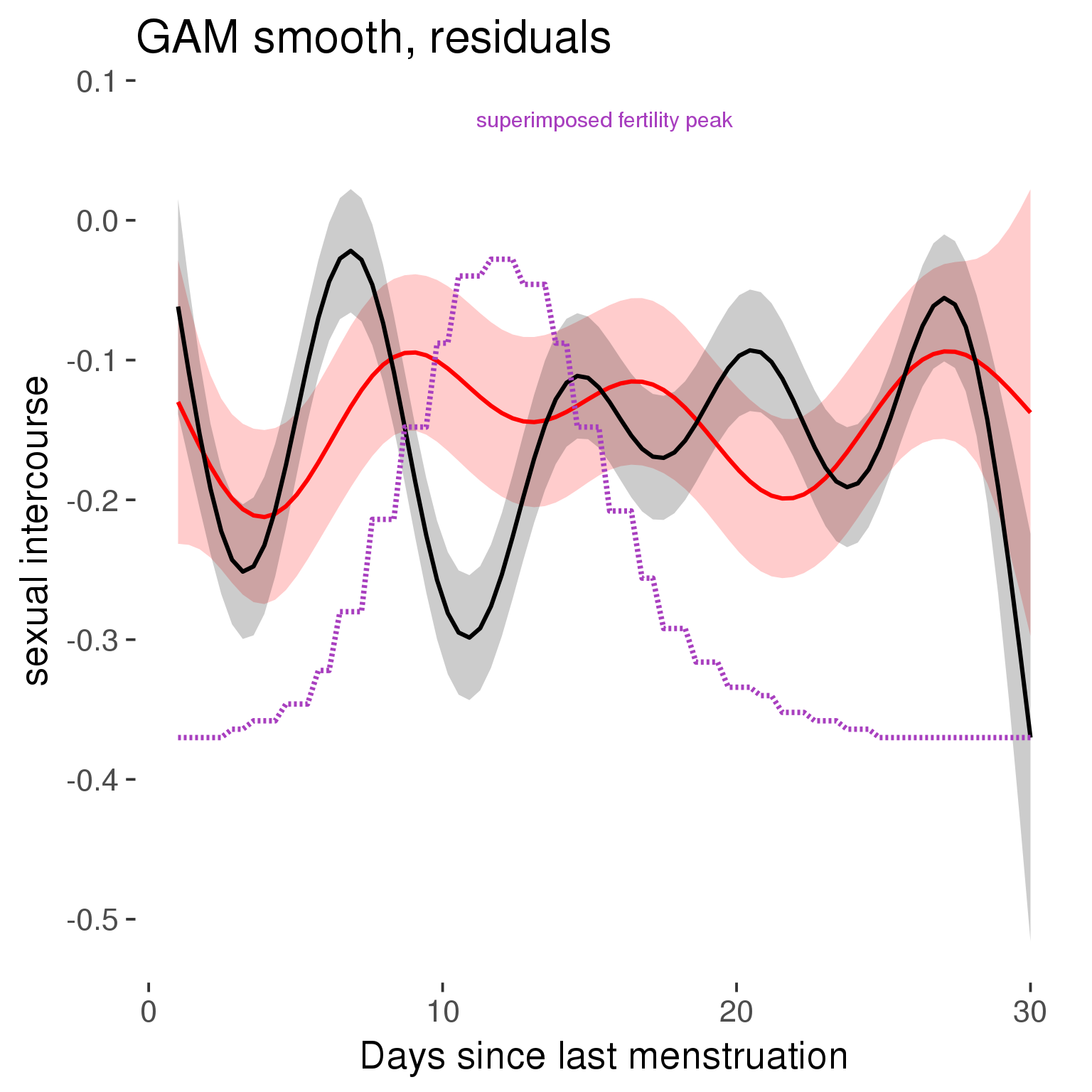
GAM smooth on raw data
As before, but without partialling anything out.
tryCatch({
trend_plot = ggplot(tmp,aes_string(x = "RCD", y = outcome, colour = "included")) +
stat_smooth(geom = 'smooth',size = 0.8, fill = "#9ECAE1", method = 'gam', formula = y ~ s(x))
}, error = function(e){cat_message(e, "danger")})
tryCatch({
trend_data = ggplot_build(trend_plot)$data[[1]]
}, error = function(e){cat_message(e, "danger")})
trend_data$RCD = round(trend_data$x)
trend_data = left_join(trend_data, tmp %>% select(real, RCD,fertile) %>% unique(), by = "RCD")
trend_data %>%
filter(real == TRUE) %>%
mutate(superimposed = ( ( (fertile - 0.01)/0.58) * (max(y)-min(y) ) ) + min(y) ) ->
trend_data
plot1b = ggplot(trend_data) +
geom_ribbon(aes(x = x, ymin = ymin, ymax = ymax, fill = factor(group)), alpha = 0.2) +
geom_line(aes(x = x, y = y, colour = factor(group)), size = 0.8, stat = "identity") +
scale_x_continuous(caption_x) +
geom_line(aes(x = x, y = superimposed), color = "#a83fbf", size = 1, linetype = 'dashed') +
annotate("text",x = mean(trend_data$x), y = max(trend_data$superimposed,na.rm=T) + 0.1, label = 'superimposed fertility peak', color = "#a83fbf") +
scale_y_continuous(outcome_label) +
ggtitle("GAM smooth, raw data") +
scale_color_manual("Contraception status",values = c("2"="black","1"= "red"), labels = c("2"="hormonally\ncontracepting","1"="cycling"), guide = F) +
scale_fill_manual("Contraception status",values = c("2"="black","1"= "red"), labels = c("2"="hormonally\ncontracepting","1"="cycling"), guide = F)
suppressWarnings(print(plot1b))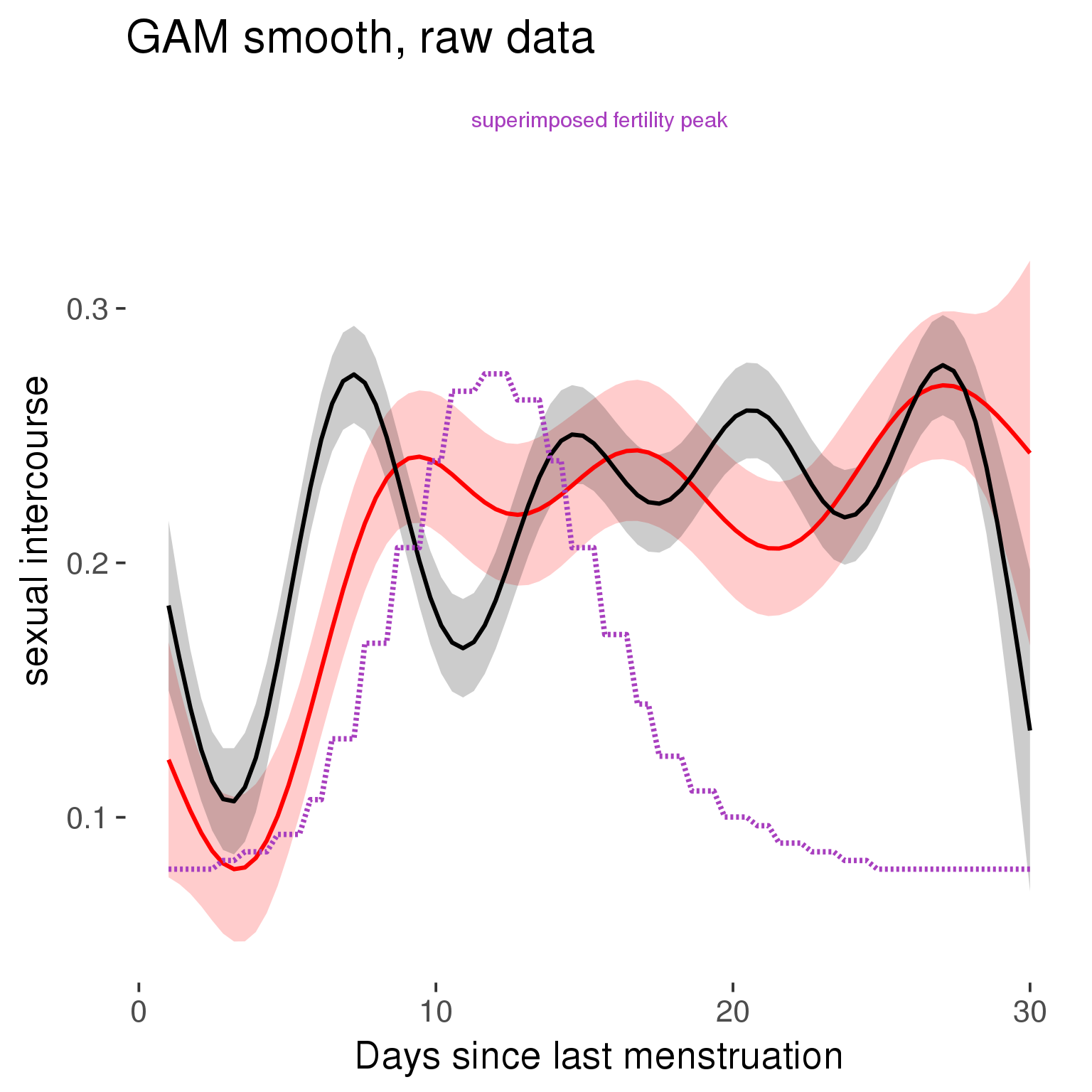
Means and standard errors over raw data
Nothing partialled out, just straight means with bootstrapped confidence intervals.
tryCatch({
trend_plot = ggplot(tmp,aes_string(x = "RCD", y = outcome, colour = "included")) +
geom_pointrange(size = 0.8, stat = 'summary', fun.data = "mean_cl_boot")
}, error = function(e){cat_message(e, "danger")})
tryCatch({
trend_data = ggplot_build(trend_plot)$data[[1]]
}, error = function(e){cat_message(e, "danger")})
trend_data$RCD = round(trend_data$x)
trend_data = left_join(trend_data, tmp %>% select(real, RCD,fertile) %>% unique(), by = "RCD")
trend_data %>%
filter(real == TRUE) %>%
mutate(superimposed = ( ( (fertile - 0.01)/0.58) * (max(y)-min(y) ) ) + min(y) ) ->
trend_data
plot3 = ggplot(trend_data) +
geom_pointrange(aes(x = x, y = y, ymin = ymin,ymax = ymax, colour = factor(group)), size = 0.8, stat = "identity", alpha = 0.6, position = position_dodge(width = .5)) +
scale_x_continuous("Days until next menstruation") +
geom_line(aes(x= x, y = superimposed), color = "#a83fbf", size = 1, linetype = 'dashed') +
annotate("text",x = mean(trend_data$x), y = max(trend_data$superimposed,na.rm=T) + 0.1, label = 'superimposed fertility peak', color = "#a83fbf") +
scale_y_continuous(outcome_label) +
ggtitle("Means with standard errors, raw data") +
scale_color_manual("Contraception status",values = c("2"="black","1"= "red"), labels = c("2"="hormonally\ncontracepting","1"="cycling"), guide = F) +
scale_fill_manual("Contraception status",values = c("2"="black","1"= "red"), labels = c("2"="hormonally\ncontracepting","1"="cycling"), guide = F)
suppressWarnings(print(plot3))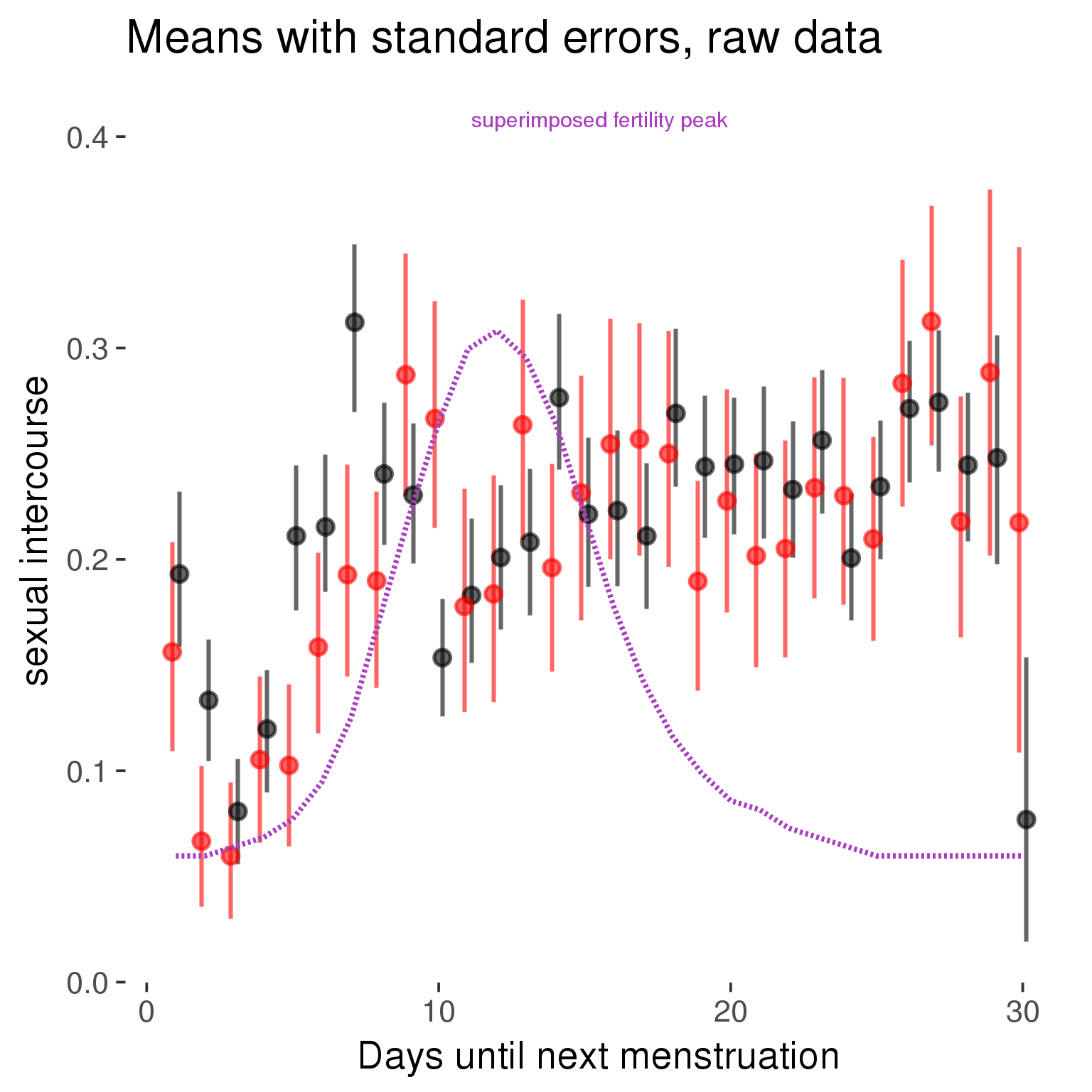
Robustness checks
M_r1: Random slopes for conception risk and menstruation
tryCatch({
# refit model with random effects for fertile and menstruation dummies
with_ind_diff = update(model, formula = . ~ . - (1| person) + (1 + fertile + menstruation | person))
# pull the random effects, format as tibble
rand = coef(with_ind_diff)$person %>%
tibble::rownames_to_column("person") %>%
mutate(person = as.numeric(person))
# pull the fixed effects
fixd = data.frame(fixef(with_ind_diff)) %>%
tibble::rownames_to_column("effect")
names(fixd) = c("effect", "pop_effect_size")
# pull apart the coefficients so that we can account for the fact that the random effect variation implicitly includes HC explaining the mean population-level effect of fertile/menstruation dummies among HC users
fixd = fixd %>%
separate(effect, c("included", "effect"), sep = ":", fill = "left") %>%
mutate(included = if_else(is.na(included), "cycling", str_replace(included, "included", "")))
fixd[2,c("included", "effect")] = c("horm_contra", "(Intercept)")
rand = rand %>%
# merge diary data on the random effects, so that we know who is a HC users and who isn't
inner_join(diary %>% select(person, included) %>% unique(), by = 'person') %>%
# gather into long format, to have the dataset by predictor
gather(effect, value, -person, -included) %>%
inner_join(fixd, by = c('effect', 'included')) %>%
# pull the fixed effects
mutate(
# only for those who are HC users, add the moderated population effect size for this effect (the random effects have the reference category mean)
value = if_else(included == "horm_contra", value + pop_effect_size, value),
effect = recode(effect, "includedhorm_contra" = "HC user",
"includedhorm_contra:fertile" = "HC user x fertile",
"includedhorm_contra:menstruationpre" = "HC user x premens.",
"includedhorm_contra:menstruationyes" = "HC user x mens.",
"menstruationyes" = "mens.",
"menstruationpre" = "premens.")) %>%
group_by(included, effect) %>%
# filter out predictors that aren't modelled as varying/random
filter(sd(value) > 0)
# plot dot plot of random effects
print(
ggplot(rand, aes(x = included, y = value, color = included, fill = included)) +
facet_wrap( ~ effect, scales = "free") +
# geom_violin(alpha = 0.4, size = 0) +
geom_dotplot(binaxis='y', dotsize = 0.1, method = "histodot") +
# geom_jitter(alpha = 0.05) +
coord_flip() +
geom_pointrange(stat = 'summary', fun.data = 'mean_sdl', color = 'darkred', size = 1.2) +
scale_color_manual("Contraception status", values = c("horm_contra"="black","cycling"= "red"), labels = c("horm_contra"="hormonally\ncontracepting","cycling"="cycling"), guide = F) +
scale_fill_manual("Contraception status", values = c("horm_contra"="black","cycling"= "red"), labels = c("horm_contra"="hormonally\ncontracepting","1"="cycling"), guide = F) +
ggtitle("M_r1: allowing participant-varying slopes", subtitle = "for the conception risk measure and the menstruation dummies") +
scale_x_discrete("Hormonal contraception", breaks = c("horm_contra", "cycling"), labels = c("yes", "no")) +
scale_y_continuous("Random effect size distribution"))
print_summary(with_ind_diff)
cat(pander(anova(model, with_ind_diff)))
}, error = function(e){
with_ind_diff = model
cat_message(e, "danger")
})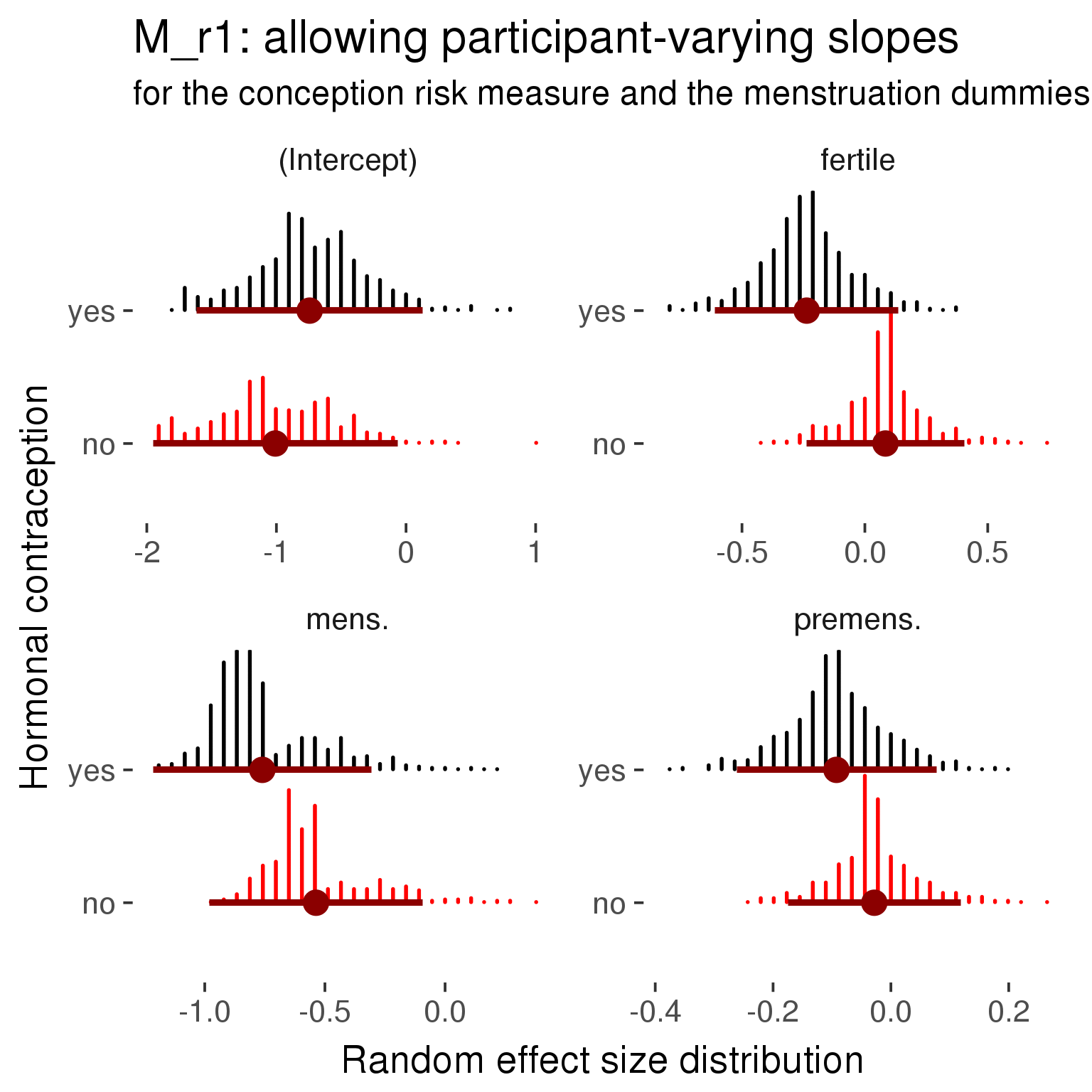
Generalized linear mixed model fit by maximum likelihood (Laplace Approximation) ['glmerMod']
Family: binomial ( probit )
Formula: had_sexual_intercourse ~ included + menstruation + fertile +
fertile_mean + (1 + fertile + menstruation | person) + included:menstruation + included:fertile
Data: diary
AIC BIC logLik deviance df.resid
25656 25811 -12809 25618 26685
Scaled residuals:
Min 1Q Median 3Q Max
-2.432 -0.542 -0.365 -0.161 4.820
Random effects:
Groups Name Variance Std.Dev. Corr
person (Intercept) 0.3335 0.578
fertile 0.2861 0.535 -0.25
menstruationpre 0.0655 0.256 -0.24 0.97
menstruationyes 0.2652 0.515 0.04 -0.05 0.09
Number of obs: 26704, groups: person, 1054
Fixed effects:
Estimate Std. Error z value Pr(>|z|)
(Intercept) -1.0404 0.0671 -15.50 < 2e-16 ***
includedhorm_contra 0.2733 0.0549 4.98 6.5e-07 ***
menstruationpre -0.0269 0.0530 -0.51 0.6116
menstruationyes -0.5579 0.0709 -7.87 3.6e-15 ***
fertile 0.0894 0.1062 0.84 0.3997
fertile_mean 0.4614 0.3063 1.51 0.1320
includedhorm_contra:menstruationpre -0.0647 0.0629 -1.03 0.3036
includedhorm_contra:menstruationyes -0.2238 0.0790 -2.83 0.0046 **
includedhorm_contra:fertile -0.3214 0.1260 -2.55 0.0108 *
---
Signif. codes: 0 '***' 0.001 '**' 0.01 '*' 0.05 '.' 0.1 ' ' 1
Correlation of Fixed Effects:
(Intr) incld_ mnstrtnp mnstrtny fertil frtl_m inclddhrm_cntr:mnstrtnp
inclddhrm_c -0.498
menstrutnpr -0.322 0.368
menstrutnys -0.175 0.213 0.249
fertile -0.304 0.451 0.498 0.243
fertile_men -0.747 -0.036 0.006 -0.011 -0.111
inclddhrm_cntr:mnstrtnp 0.264 -0.462 -0.788 -0.201 -0.400 -0.014
inclddhrm_cntr:mnstrtny 0.157 -0.277 -0.212 -0.678 -0.202 -0.005 0.269
inclddhrm_cntr:f 0.295 -0.565 -0.402 -0.193 -0.785 0.017 0.514
inclddhrm_cntr:mnstrtny
inclddhrm_c
menstrutnpr
menstrutnys
fertile
fertile_men
inclddhrm_cntr:mnstrtnp
inclddhrm_cntr:mnstrtny
inclddhrm_cntr:f 0.257
convergence code: 0
Model failed to converge with max|grad| = 0.586369 (tol = 0.001, component 1)
| Df | AIC | BIC | logLik | deviance | Chisq | Chi Df | Pr(>Chisq) | |
|---|---|---|---|---|---|---|---|---|
| model | 10 | 25699 | 25780 | -12839 | 25679 | NA | NA | NA |
| with_ind_diff | 19 | 25656 | 25811 | -12809 | 25618 | 60.85 | 9 | 0.0000000009197 |
robustness_check_ovu_shift(model, diary)M_e: Exclusion criteria
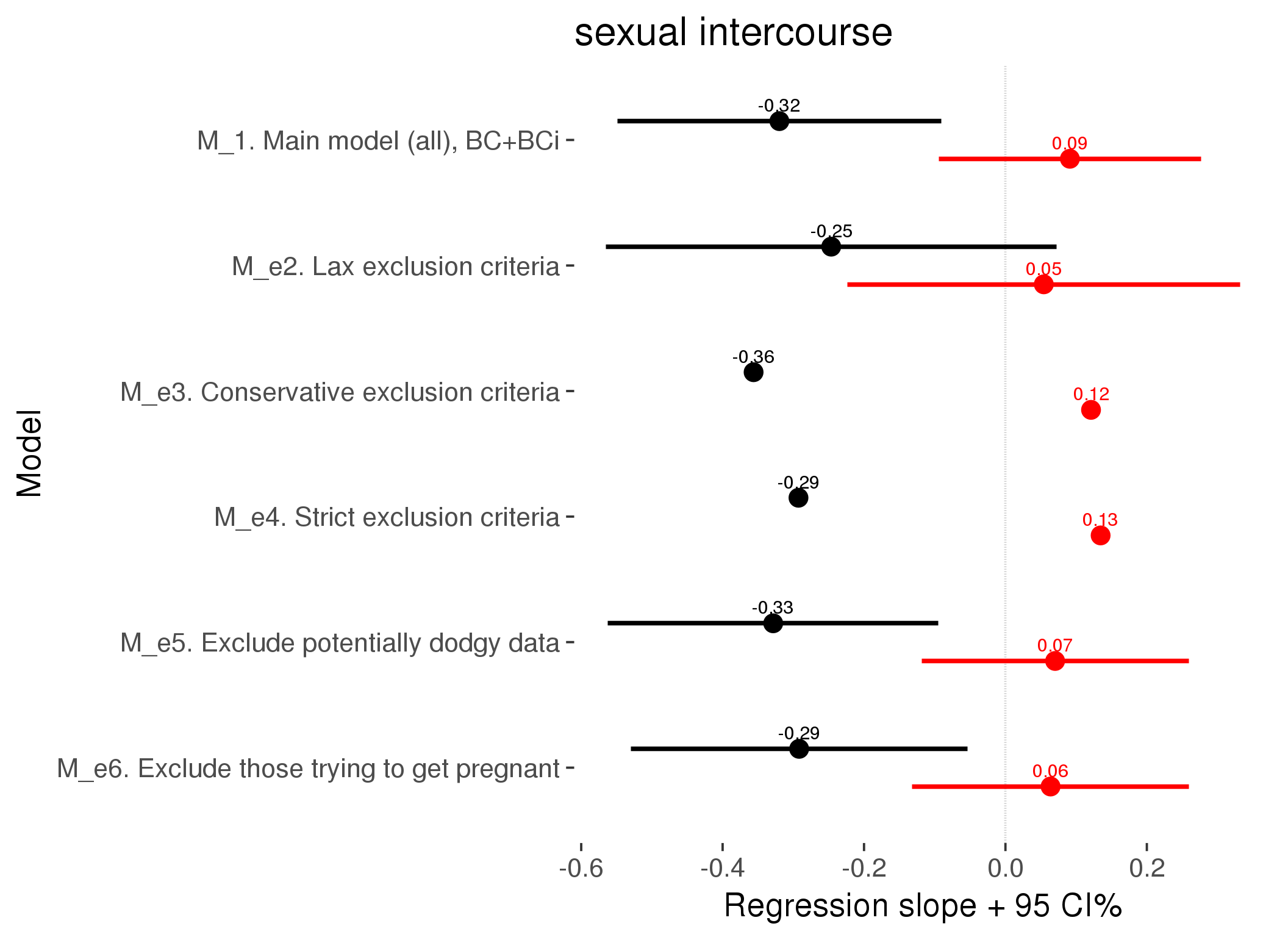
M_p: Predictors
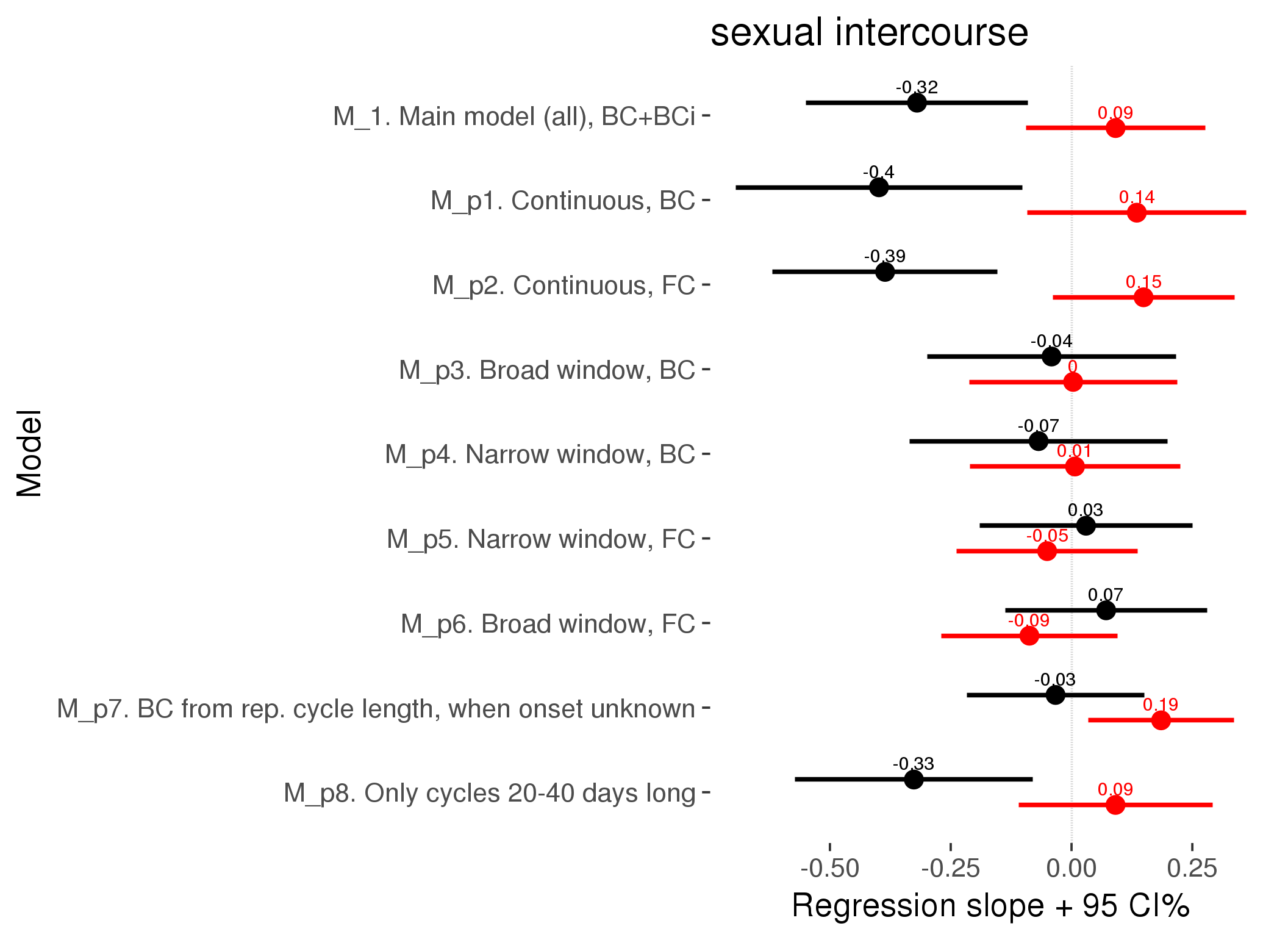
M_c: Covariates, controls, autocorrelation
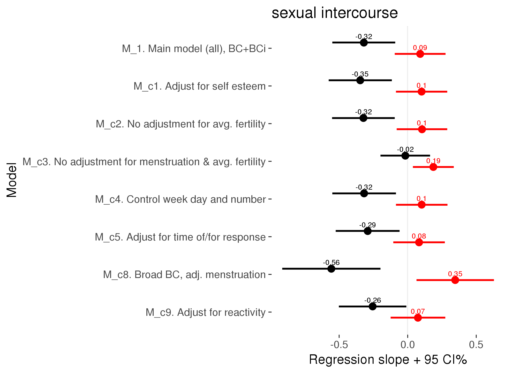
Generalized linear mixed model fit by maximum likelihood (Laplace Approximation) ['glmerMod']
Family: binomial ( probit )
AIC BIC logLik deviance df.resid
23070 23216 -11517 23034 24380
Scaled residuals:
Min 1Q Median 3Q Max
-2.473 -0.534 -0.366 -0.186 6.565
Random effects:
Groups Name Variance Std.Dev.
person (Intercept) 0.3091508 0.55601
Xr.2 s(days_filled_out):includedhorm_contra 0.1906540 0.43664
Xr.1 s(days_filled_out):includedcycling 0.0000078 0.00279
Xr.0 s(day_number):includedhorm_contra 0.2608332 0.51072
Xr s(day_number):includedcycling 0.0000127 0.00356
Number of obs: 24398, groups: person, 1054; Xr.2, 8; Xr.1, 8; Xr.0, 8; Xr, 8
Fixed effects:
Estimate Std. Error z value Pr(>|z|)
X(Intercept) -1.0896 0.0669 -16.28 < 2e-16 ***
Xincludedhorm_contra 0.2519 0.0556 4.53 0.000006 ***
Xmenstruationpre -0.0056 0.0493 -0.11 0.90967
Xmenstruationyes -0.4325 0.0517 -8.36 < 2e-16 ***
Xfertile 0.0747 0.1017 0.73 0.46257
Xfertile_mean 0.5420 0.3043 1.78 0.07489 .
Xincludedhorm_contra:menstruationpre -0.0562 0.0617 -0.91 0.36223
Xincludedhorm_contra:menstruationyes -0.1871 0.0672 -2.79 0.00535 **
Xincludedhorm_contra:fertile -0.2556 0.1257 -2.03 0.04203 *
Xs(day_number):includedcyclingFx1 0.3015 0.0687 4.39 0.000012 ***
Xs(day_number):includedhorm_contraFx1 0.8159 0.2729 2.99 0.00279 **
Xs(days_filled_out):includedcyclingFx1 -0.2657 0.0709 -3.75 0.00018 ***
Xs(days_filled_out):includedhorm_contraFx1 -0.5657 0.1862 -3.04 0.00239 **
---
Signif. codes: 0 '***' 0.001 '**' 0.01 '*' 0.05 '.' 0.1 ' ' 1
Family: binomial
Link function: probit
Formula:
had_sexual_intercourse ~ included + menstruation + fertile +
fertile_mean + s(day_number, by = included) + s(days_filled_out,
by = included) + included:menstruation + included:fertile
Parametric coefficients:
Estimate Std. Error z value Pr(>|z|)
(Intercept) -1.0896 0.0654 -16.65 < 2e-16 ***
includedhorm_contra 0.2519 0.0548 4.60 0.0000043 ***
menstruationpre -0.0056 0.0485 -0.12 0.9081
menstruationyes -0.4325 0.0511 -8.46 < 2e-16 ***
fertile 0.0747 0.0998 0.75 0.4540
fertile_mean 0.5420 0.2977 1.82 0.0687 .
includedhorm_contra:menstruationpre -0.0562 0.0607 -0.93 0.3542
includedhorm_contra:menstruationyes -0.1871 0.0665 -2.81 0.0049 **
includedhorm_contra:fertile -0.2556 0.1234 -2.07 0.0384 *
---
Signif. codes: 0 '***' 0.001 '**' 0.01 '*' 0.05 '.' 0.1 ' ' 1
Approximate significance of smooth terms:
edf Ref.df Chi.sq p-value
s(day_number):includedcycling 1.00 1.00 20.1 7.5e-06 ***
s(day_number):includedhorm_contra 4.28 4.28 64.0 1.4e-12 ***
s(days_filled_out):includedcycling 1.00 1.00 14.6 0.00013 ***
s(days_filled_out):includedhorm_contra 3.83 3.83 61.4 2.2e-12 ***
---
Signif. codes: 0 '***' 0.001 '**' 0.01 '*' 0.05 '.' 0.1 ' ' 1
R-sq.(adj) = 0.0162
glmer.ML = 20982 Scale est. = 1 n = 24398
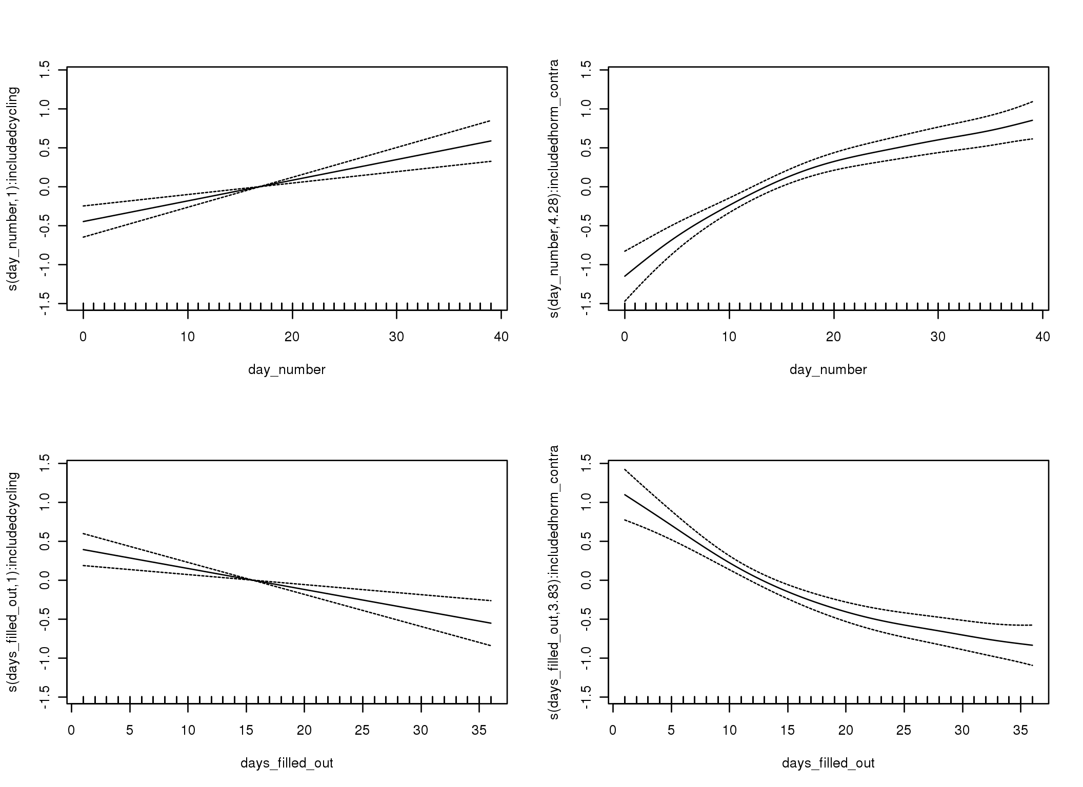
M_d: Other designs
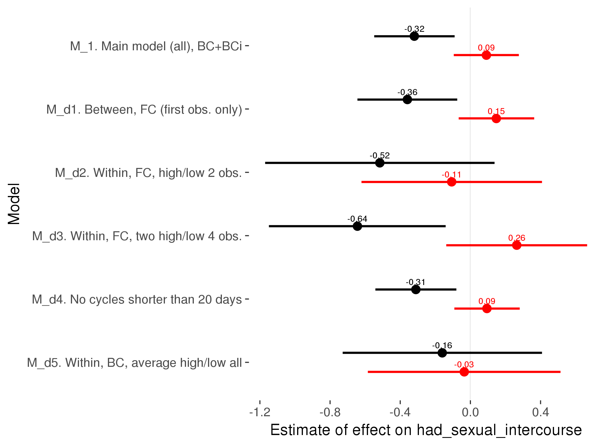
M_m1: Moderation by contraceptive method
Based on the sample with lax exclusion criteria. Users who used any hormonal contraception are classified as hormonal, users who use any awareness-based methods (counting, temperature-based) are classified as ‘fertility-awareness’, women who don’t fall into the before groups and use condoms, pessars, coitus interruptus etc. are classified as ‘barrie or abstinence’. Women who don’t use contraception or use other methods such as sterilisation are excluded from this analysis.
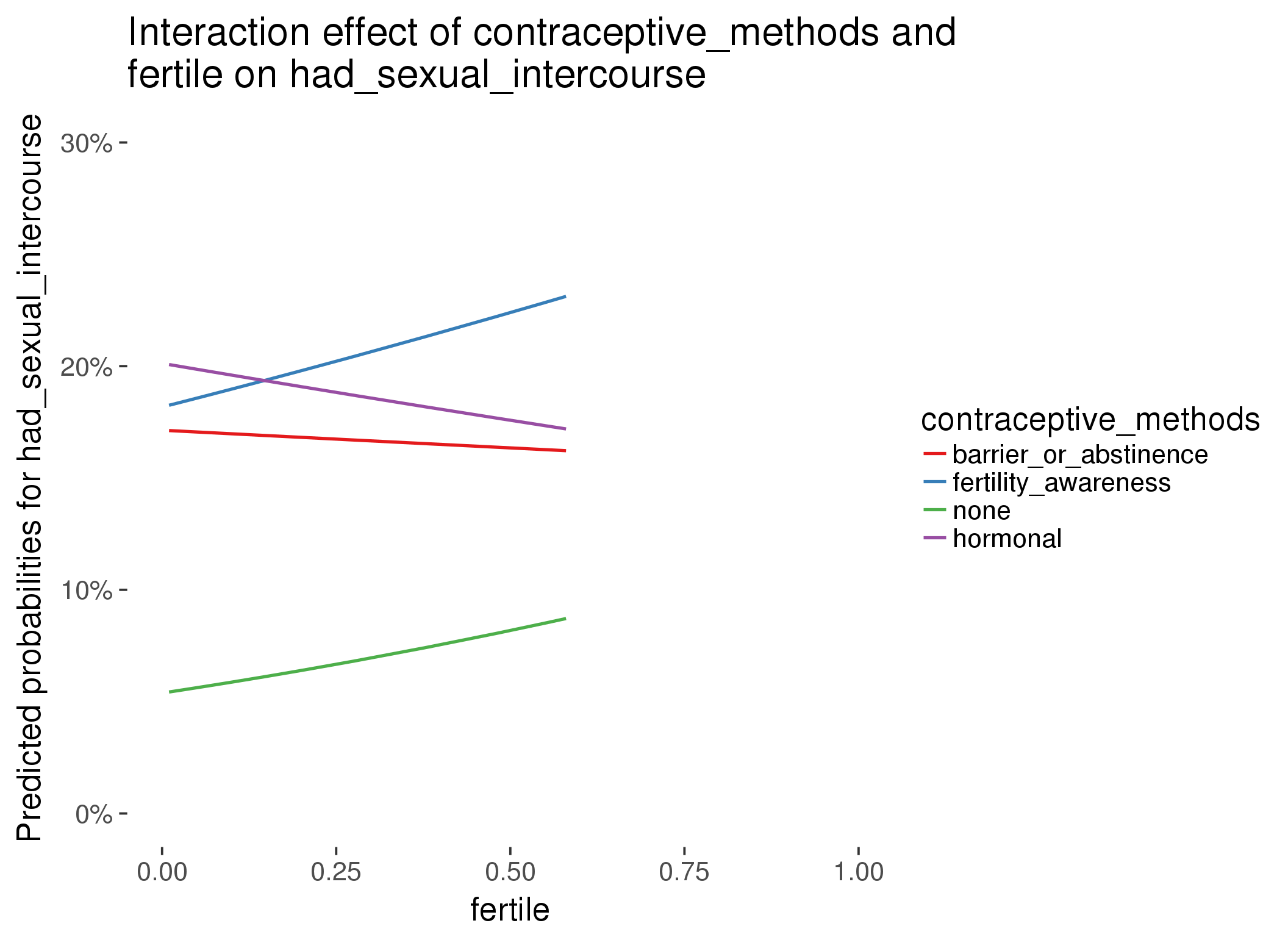
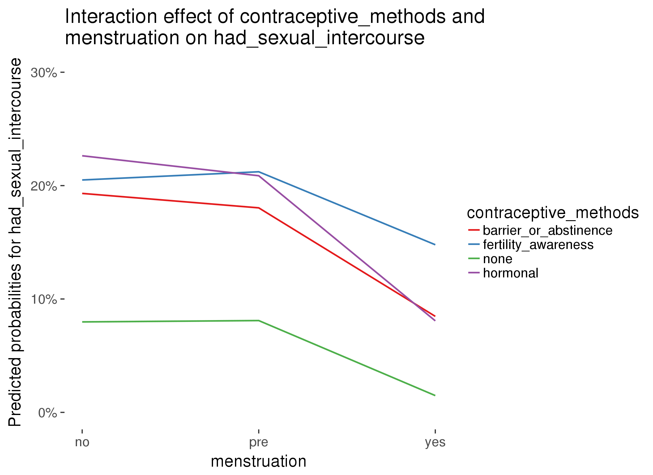
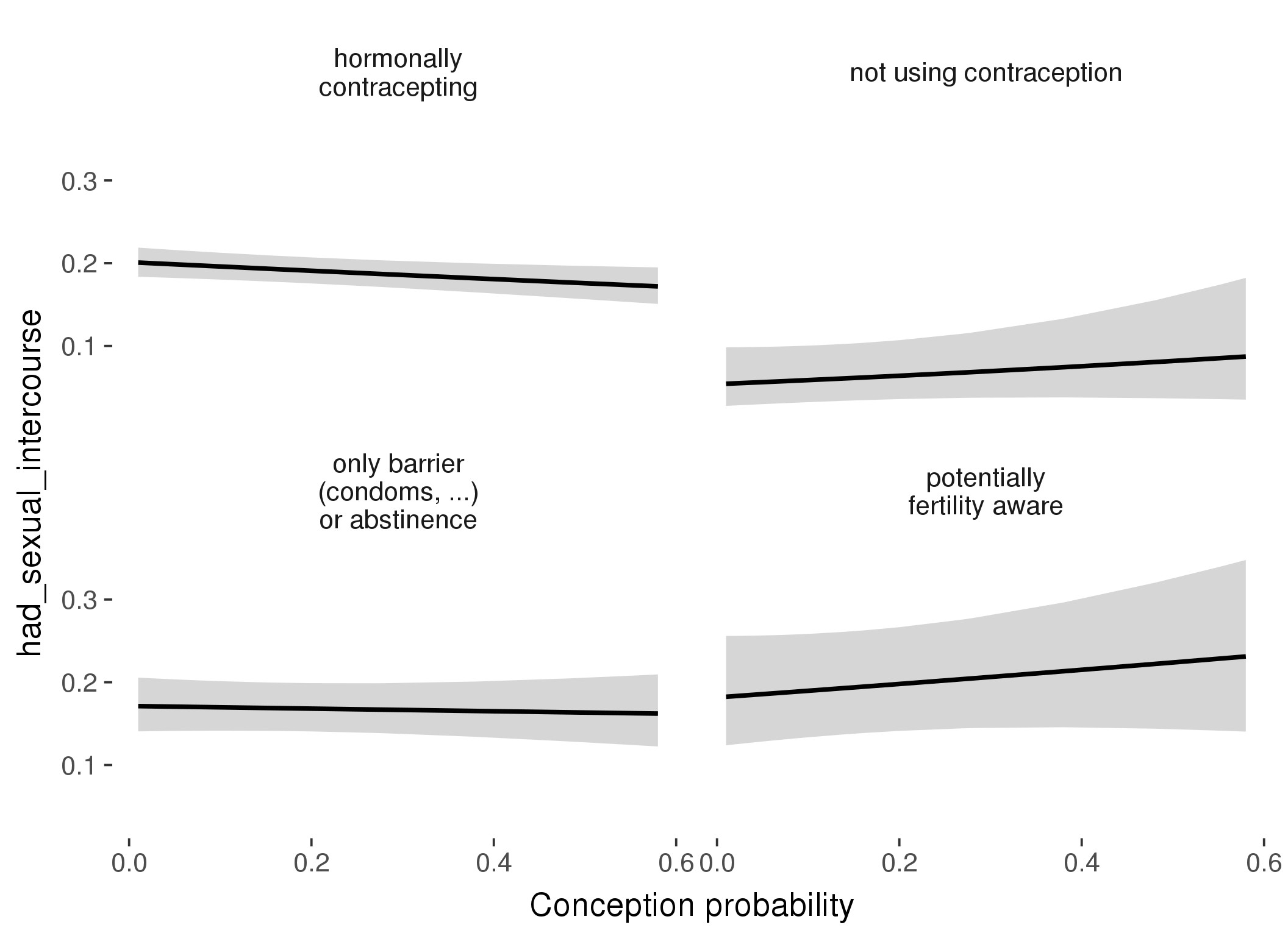
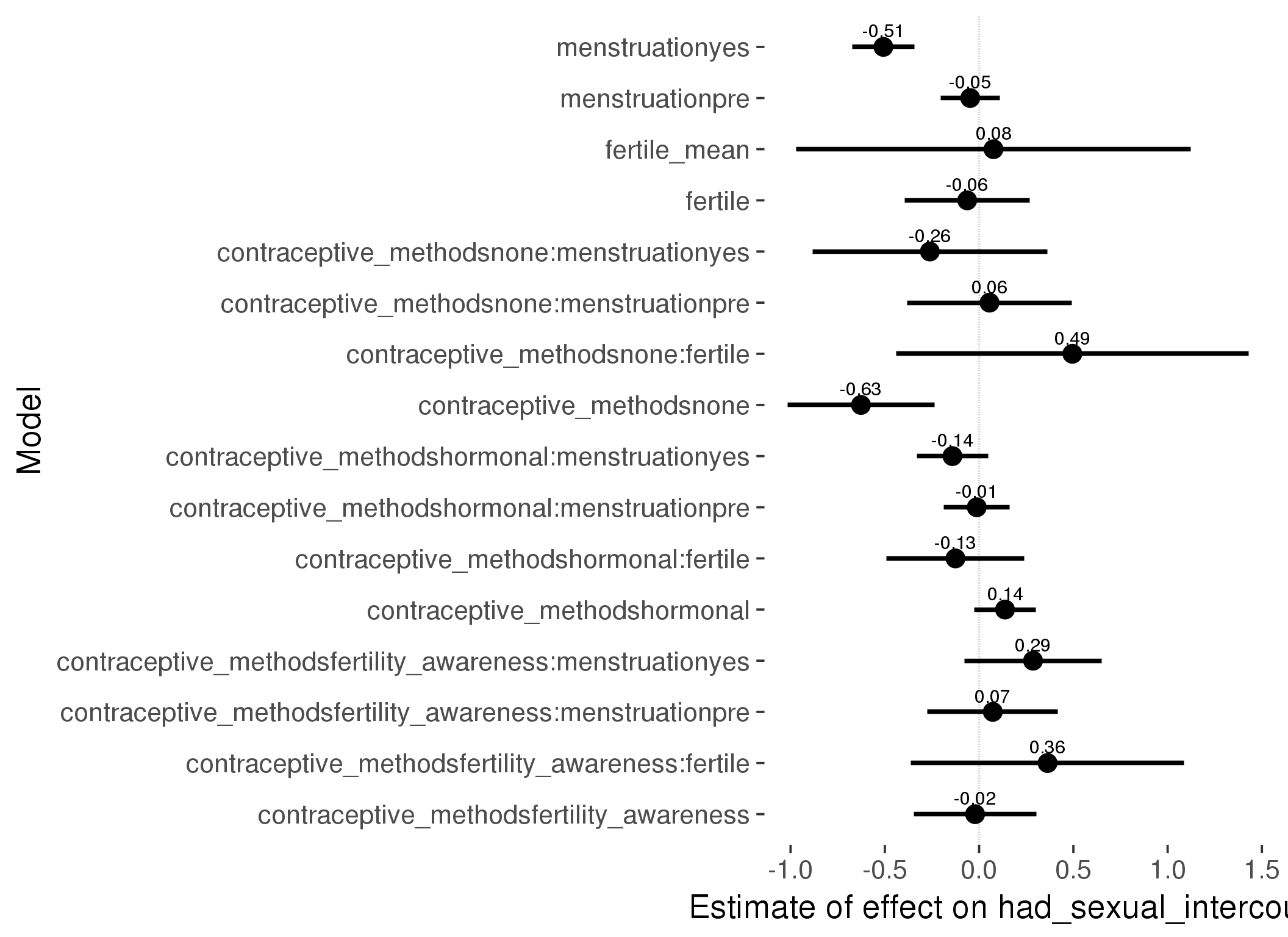
Generalized linear mixed model fit by maximum likelihood (Laplace Approximation) ['glmerMod']
Family: binomial ( probit )
Formula: had_sexual_intercourse ~ fertile_mean + (1 | person) + contraceptive_methods +
fertile + menstruation + fertile:contraceptive_methods + menstruation:contraceptive_methods
Data: diary
Subset: !is.na(included_lax) & contraceptive_method != "other"
AIC BIC logLik deviance df.resid
16493 16632 -8228 16457 17026
Scaled residuals:
Min 1Q Median 3Q Max
-2.091 -0.552 -0.389 -0.184 6.450
Random effects:
Groups Name Variance Std.Dev.
person (Intercept) 0.243 0.493
Number of obs: 17044, groups: person, 513
Fixed effects:
Estimate Std. Error z value Pr(>|z|)
(Intercept) -0.8688 0.1144 -7.59 3.1e-14 ***
fertile_mean 0.0762 0.5340 0.14 0.8865
contraceptive_methodsfertility_awareness -0.0212 0.1665 -0.13 0.8988
contraceptive_methodsnone -0.6267 0.1987 -3.15 0.0016 **
contraceptive_methodshormonal 0.1375 0.0833 1.65 0.0987 .
fertile -0.0632 0.1689 -0.37 0.7083
menstruationpre -0.0474 0.0799 -0.59 0.5532
menstruationyes -0.5077 0.0847 -5.99 2.1e-09 ***
contraceptive_methodsfertility_awareness:fertile 0.3631 0.3700 0.98 0.3264
contraceptive_methodsnone:fertile 0.4947 0.4773 1.04 0.2999
contraceptive_methodshormonal:fertile -0.1254 0.1868 -0.67 0.5020
contraceptive_methodsfertility_awareness:menstruationpre 0.0726 0.1767 0.41 0.6809
contraceptive_methodsnone:menstruationpre 0.0553 0.2227 0.25 0.8039
contraceptive_methodshormonal:menstruationpre -0.0125 0.0893 -0.14 0.8885
contraceptive_methodsfertility_awareness:menstruationyes 0.2860 0.1860 1.54 0.1242
contraceptive_methodsnone:menstruationyes -0.2611 0.3173 -0.82 0.4105
contraceptive_methodshormonal:menstruationyes -0.1414 0.0967 -1.46 0.1436
---
Signif. codes: 0 '***' 0.001 '**' 0.01 '*' 0.05 '.' 0.1 ' ' 1
convergence code: 0
Model failed to converge with max|grad| = 0.150687 (tol = 0.001, component 1)
| Df | AIC | BIC | logLik | deviance | Chisq | Chi Df | Pr(>Chisq) | |
|---|---|---|---|---|---|---|---|---|
| add_main | 12 | 16486 | 16579 | -8231 | 16462 | NA | NA | NA |
| by_method | 18 | 16493 | 16632 | -8228 | 16457 | 5.269 | 6 | 0.5098 |
M_m2: Moderation by participant age
model %>%
test_moderator("age_group", diary, xlevels = 5)| Df | AIC | BIC | logLik | deviance | Chisq | Chi Df | Pr(>Chisq) | |
|---|---|---|---|---|---|---|---|---|
| with_main | 18 | 25696 | 25843 | -12830 | 25660 | NA | NA | NA |
| with_mod | 26 | 25700 | 25913 | -12824 | 25648 | 12.3 | 8 | 0.1382 |
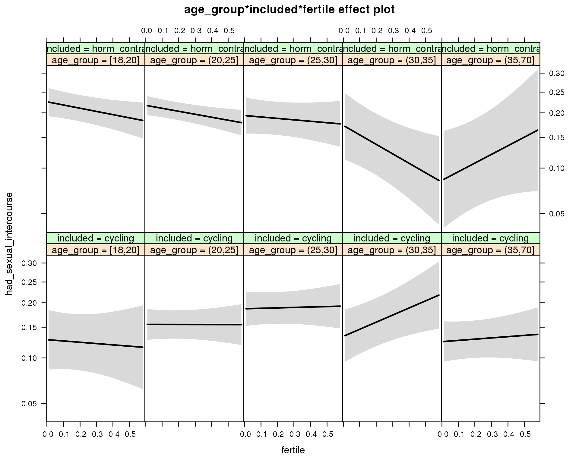
Generalized linear mixed model fit by maximum likelihood (Laplace Approximation) ['glmerMod']
Family: binomial ( probit )
Formula: had_sexual_intercourse ~ menstruation + fertile_mean + (1 | person) +
age_group + included + fertile + menstruation:included +
age_group:included + age_group:fertile + included:fertile + age_group:included:fertile
Data: diary
AIC BIC logLik deviance df.resid
25700 25912 -12824 25648 26678
Scaled residuals:
Min 1Q Median 3Q Max
-2.987 -0.544 -0.377 -0.181 6.044
Random effects:
Groups Name Variance Std.Dev.
person (Intercept) 0.304 0.551
Number of obs: 26704, groups: person, 1054
Fixed effects:
Estimate Std. Error z value Pr(>|z|)
(Intercept) -1.12874 0.13088 -8.62 < 2e-16 ***
menstruationpre -0.02299 0.04699 -0.49 0.62465
menstruationyes -0.41442 0.04786 -8.66 < 2e-16 ***
fertile_mean 0.39930 0.29873 1.34 0.18133
age_group(20,25] 0.12134 0.13646 0.89 0.37389
age_group(25,30] 0.24649 0.13997 1.76 0.07824 .
age_group(30,35] 0.02627 0.16168 0.16 0.87095
age_group(35,70] -0.01590 0.14644 -0.11 0.91352
includedhorm_contra 0.43191 0.13737 3.14 0.00167 **
fertile -0.10386 0.29664 -0.35 0.72624
menstruationpre:includedhorm_contra -0.06780 0.05876 -1.15 0.24856
menstruationyes:includedhorm_contra -0.20899 0.06221 -3.36 0.00078 ***
age_group(20,25]:includedhorm_contra -0.14959 0.15318 -0.98 0.32880
age_group(25,30]:includedhorm_contra -0.35613 0.16827 -2.12 0.03431 *
age_group(30,35]:includedhorm_contra -0.21436 0.21930 -0.98 0.32835
age_group(35,70]:includedhorm_contra -0.61057 0.25452 -2.40 0.01644 *
age_group(20,25]:fertile 0.10196 0.32347 0.32 0.75260
age_group(25,30]:fertile 0.13897 0.32830 0.42 0.67208
age_group(30,35]:fertile 0.67145 0.37524 1.79 0.07355 .
age_group(35,70]:fertile 0.20389 0.34680 0.59 0.55659
includedhorm_contra:fertile -0.15236 0.32078 -0.47 0.63480
age_group(20,25]:includedhorm_contra:fertile -0.08346 0.35374 -0.24 0.81348
age_group(25,30]:includedhorm_contra:fertile 0.00287 0.38240 0.01 0.99402
age_group(30,35]:includedhorm_contra:fertile -1.17268 0.50531 -2.32 0.02030 *
age_group(35,70]:includedhorm_contra:fertile 0.74198 0.57629 1.29 0.19792
---
Signif. codes: 0 '***' 0.001 '**' 0.01 '*' 0.05 '.' 0.1 ' ' 1
convergence code: 0
Model failed to converge with max|grad| = 0.214259 (tol = 0.001, component 1)
M_m3: Moderation by weekend
model %>%
test_moderator("weekend", diary, xlevels = 2) | Df | AIC | BIC | logLik | deviance | Chisq | Chi Df | Pr(>Chisq) | |
|---|---|---|---|---|---|---|---|---|
| with_main | 12 | 25420 | 25519 | -12698 | 25396 | NA | NA | NA |
| with_mod | 14 | 25424 | 25538 | -12698 | 25396 | 0.6656 | 2 | 0.7169 |
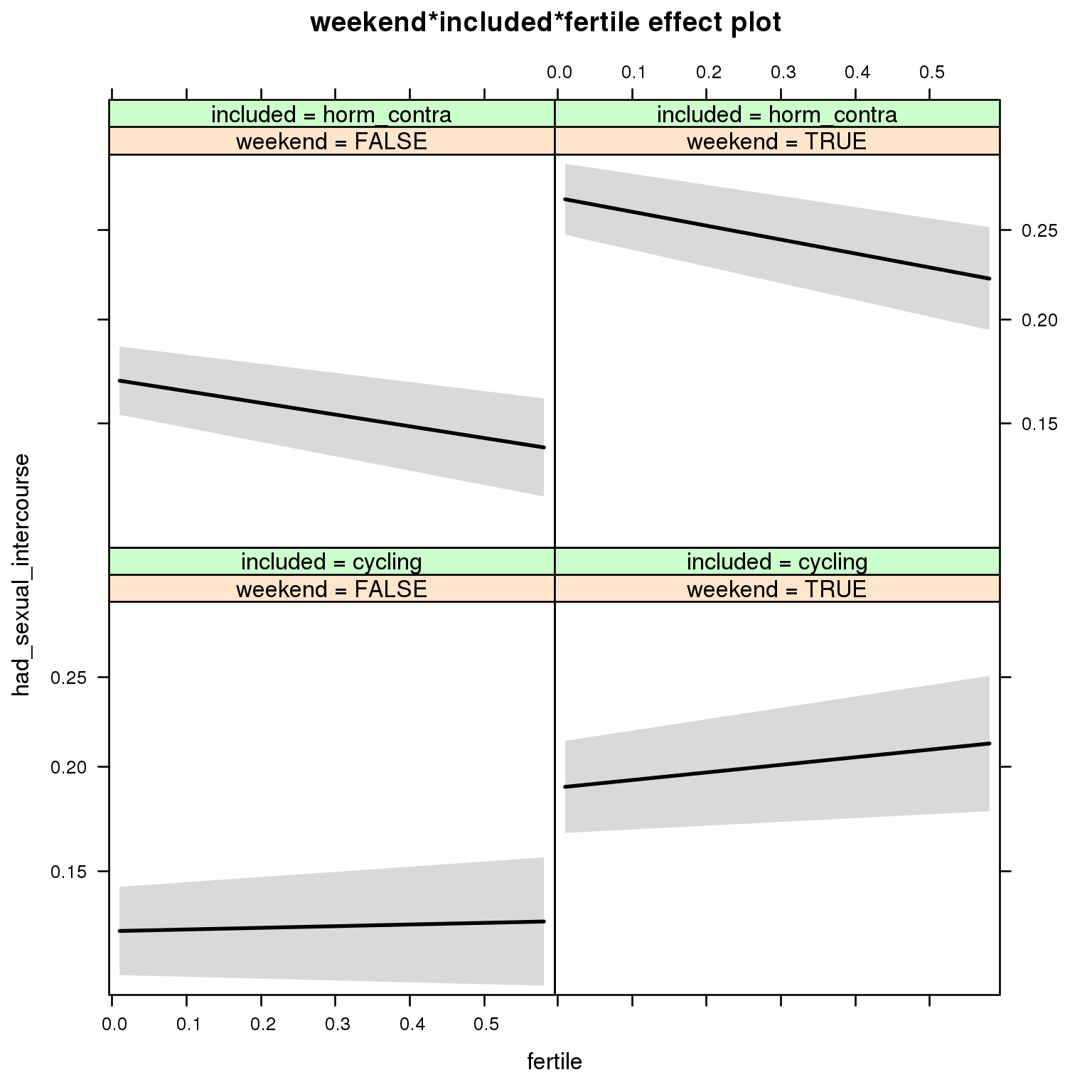
Generalized linear mixed model fit by maximum likelihood (Laplace Approximation) ['glmerMod']
Family: binomial ( probit )
Formula: had_sexual_intercourse ~ menstruation + fertile_mean + (1 | person) +
weekend + included + fertile + menstruation:included + weekend:included +
weekend:fertile + included:fertile + weekend:included:fertile
Data: diary
AIC BIC logLik deviance df.resid
25424 25538 -12698 25396 26690
Scaled residuals:
Min 1Q Median 3Q Max
-2.739 -0.536 -0.362 -0.165 6.169
Random effects:
Groups Name Variance Std.Dev.
person (Intercept) 0.321 0.566
Number of obs: 26704, groups: person, 1054
Fixed effects:
Estimate Std. Error z value Pr(>|z|)
(Intercept) -1.1427 0.0685 -16.68 < 2e-16 ***
menstruationpre -0.0246 0.0472 -0.52 0.60244
menstruationyes -0.4209 0.0481 -8.75 < 2e-16 ***
fertile_mean 0.4152 0.3036 1.37 0.17144
weekendTRUE 0.2680 0.0420 6.38 0.00000000018 ***
includedhorm_contra 0.2430 0.0588 4.13 0.00003568475 ***
fertile 0.0309 0.1194 0.26 0.79553
menstruationpre:includedhorm_contra -0.0712 0.0591 -1.21 0.22810
menstruationyes:includedhorm_contra -0.2074 0.0626 -3.31 0.00092 ***
weekendTRUE:includedhorm_contra 0.0712 0.0528 1.35 0.17743
weekendTRUE:fertile 0.1110 0.1587 0.70 0.48422
includedhorm_contra:fertile -0.2497 0.1485 -1.68 0.09274 .
weekendTRUE:includedhorm_contra:fertile -0.1524 0.1984 -0.77 0.44240
---
Signif. codes: 0 '***' 0.001 '**' 0.01 '*' 0.05 '.' 0.1 ' ' 1
convergence code: 0
Model failed to converge with max|grad| = 0.0364538 (tol = 0.001, component 1)
M_m4: Moderation by weekday
model %>%
test_moderator("weekday", diary, xlevels = 7)| Df | AIC | BIC | logLik | deviance | Chisq | Chi Df | Pr(>Chisq) | |
|---|---|---|---|---|---|---|---|---|
| with_main | 22 | 25221 | 25401 | -12589 | 25177 | NA | NA | NA |
| with_mod | 34 | 25237 | 25516 | -12585 | 25169 | 8.088 | 12 | 0.7783 |
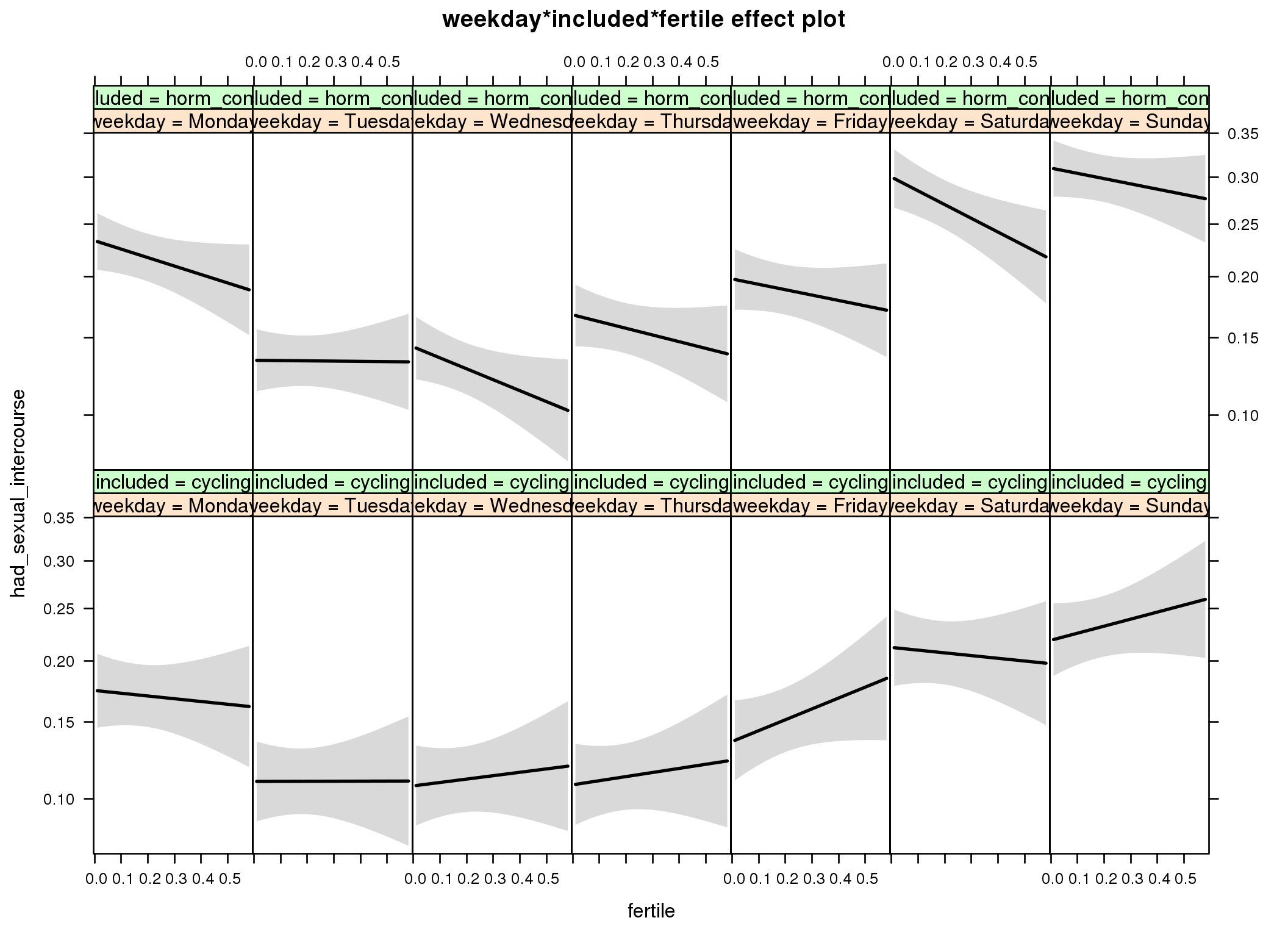
Generalized linear mixed model fit by maximum likelihood (Laplace Approximation) ['glmerMod']
Family: binomial ( probit )
Formula: had_sexual_intercourse ~ menstruation + fertile_mean + (1 | person) +
weekday + included + fertile + menstruation:included + weekday:included +
weekday:fertile + included:fertile + weekday:included:fertile
Data: diary
AIC BIC logLik deviance df.resid
25237 25516 -12585 25169 26670
Scaled residuals:
Min 1Q Median 3Q Max
-3.108 -0.530 -0.353 -0.154 6.014
Random effects:
Groups Name Variance Std.Dev.
person (Intercept) 0.328 0.573
Number of obs: 26704, groups: person, 1054
Fixed effects:
Estimate Std. Error z value Pr(>|z|)
(Intercept) -0.92677 0.08178 -11.33 < 2e-16 ***
menstruationpre -0.02366 0.04744 -0.50 0.61802
menstruationyes -0.42415 0.04832 -8.78 < 2e-16 ***
fertile_mean 0.39517 0.30629 1.29 0.19699
weekdayTuesday -0.28962 0.07738 -3.74 0.00018 ***
weekdayWednesday -0.30379 0.07761 -3.91 0.000091 ***
weekdayThursday -0.30031 0.07854 -3.82 0.00013 ***
weekdayFriday -0.16246 0.07769 -2.09 0.03652 *
weekdaySaturday 0.13711 0.07539 1.82 0.06899 .
weekdaySunday 0.16002 0.07251 2.21 0.02732 *
includedhorm_contra 0.25776 0.08077 3.19 0.00142 **
fertile -0.08773 0.20667 -0.42 0.67119
menstruationpre:includedhorm_contra -0.07253 0.05940 -1.22 0.22212
menstruationyes:includedhorm_contra -0.20494 0.06287 -3.26 0.00112 **
weekdayTuesday:includedhorm_contra -0.09131 0.09771 -0.93 0.35007
weekdayWednesday:includedhorm_contra -0.03460 0.09815 -0.35 0.72442
weekdayThursday:includedhorm_contra 0.06410 0.09852 0.65 0.51526
weekdayFriday:includedhorm_contra 0.04062 0.09737 0.42 0.67654
weekdaySaturday:includedhorm_contra 0.06527 0.09469 0.69 0.49062
weekdaySunday:includedhorm_contra 0.07127 0.09146 0.78 0.43580
weekdayTuesday:fertile 0.08984 0.29514 0.30 0.76082
weekdayWednesday:fertile 0.19594 0.29618 0.66 0.50826
weekdayThursday:fertile 0.21843 0.30161 0.72 0.46893
weekdayFriday:fertile 0.43408 0.29088 1.49 0.13563
weekdaySaturday:fertile 0.00121 0.28769 0.00 0.99663
weekdaySunday:fertile 0.31208 0.27733 1.13 0.26047
includedhorm_contra:fertile -0.18168 0.25796 -0.70 0.48125
weekdayTuesday:includedhorm_contra:fertile 0.17132 0.36950 0.46 0.64290
weekdayWednesday:includedhorm_contra:fertile -0.27482 0.37412 -0.73 0.46260
weekdayThursday:includedhorm_contra:fertile -0.16265 0.37491 -0.43 0.66440
weekdayFriday:includedhorm_contra:fertile -0.33598 0.36348 -0.92 0.35531
weekdaySaturday:includedhorm_contra:fertile -0.16912 0.35933 -0.47 0.63789
weekdaySunday:includedhorm_contra:fertile -0.21064 0.34715 -0.61 0.54401
---
Signif. codes: 0 '***' 0.001 '**' 0.01 '*' 0.05 '.' 0.1 ' ' 1
convergence code: 0
Model failed to converge with max|grad| = 0.0370517 (tol = 0.001, component 1)
failure to converge in 10000 evaluations
M_m5: Moderation by exclusion threshold
model %>%
test_moderator("included_levels", diary, xlevels = 4)| Df | AIC | BIC | logLik | deviance | Chisq | Chi Df | Pr(>Chisq) | |
|---|---|---|---|---|---|---|---|---|
| with_main | 16 | 25701 | 25832 | -12835 | 25669 | NA | NA | NA |
| with_mod | 22 | 25712 | 25892 | -12834 | 25668 | 1.381 | 6 | 0.967 |
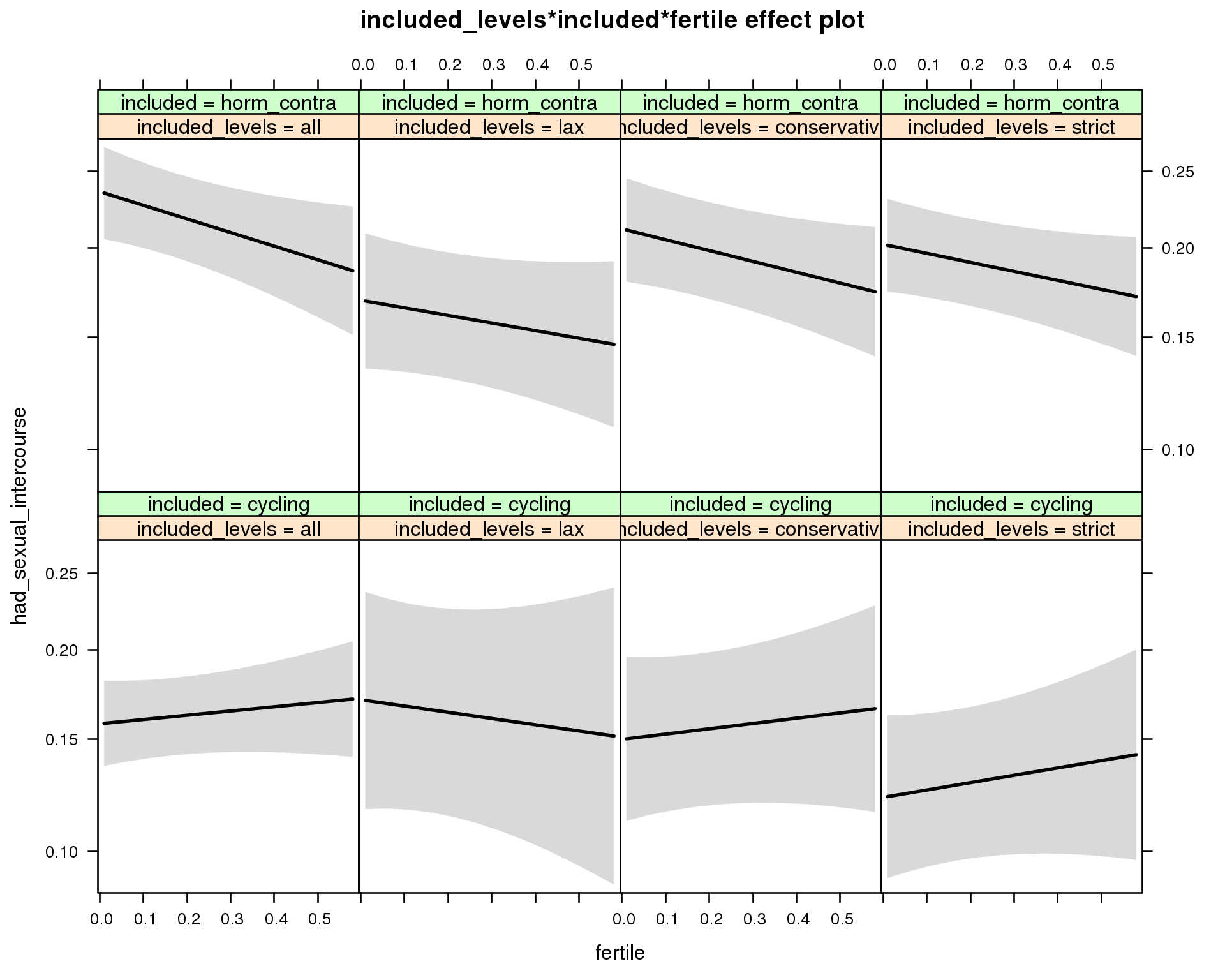
Generalized linear mixed model fit by maximum likelihood (Laplace Approximation) ['glmerMod']
Family: binomial ( probit )
Formula: had_sexual_intercourse ~ menstruation + fertile_mean + (1 | person) +
included_levels + included + fertile + menstruation:included +
included_levels:included + included_levels:fertile + included:fertile +
included_levels:included:fertile
Data: diary
AIC BIC logLik deviance df.resid
25712 25892 -12834 25668 26682
Scaled residuals:
Min 1Q Median 3Q Max
-2.618 -0.545 -0.376 -0.187 6.203
Random effects:
Groups Name Variance Std.Dev.
person (Intercept) 0.305 0.552
Number of obs: 26704, groups: person, 1054
Fixed effects:
Estimate Std. Error z value Pr(>|z|)
(Intercept) -1.0088 0.0717 -14.06 < 2e-16 ***
menstruationpre -0.0223 0.0470 -0.47 0.63575
menstruationyes -0.4130 0.0478 -8.64 < 2e-16 ***
fertile_mean 0.4704 0.3022 1.56 0.11958
included_levelslax 0.0523 0.1302 0.40 0.68783
included_levelsconservative -0.0341 0.1028 -0.33 0.74035
included_levelsstrict -0.1606 0.1023 -1.57 0.11646
includedhorm_contra 0.3327 0.0738 4.51 0.0000066 ***
fertile 0.0928 0.1185 0.78 0.43362
menstruationpre:includedhorm_contra -0.0656 0.0588 -1.11 0.26488
menstruationyes:includedhorm_contra -0.2095 0.0622 -3.37 0.00076 ***
included_levelslax:includedhorm_contra -0.2892 0.1596 -1.81 0.06997 .
included_levelsconservative:includedhorm_contra -0.0472 0.1288 -0.37 0.71375
included_levelsstrict:includedhorm_contra 0.0455 0.1257 0.36 0.71743
included_levelslax:fertile -0.2289 0.2950 -0.78 0.43789
included_levelsconservative:fertile 0.0228 0.2163 0.11 0.91608
included_levelsstrict:fertile 0.0677 0.2234 0.30 0.76197
includedhorm_contra:fertile -0.3903 0.1752 -2.23 0.02591 *
included_levelslax:includedhorm_contra:fertile 0.3604 0.3545 1.02 0.30931
included_levelsconservative:includedhorm_contra:fertile 0.0382 0.2756 0.14 0.88972
included_levelsstrict:includedhorm_contra:fertile 0.0334 0.2773 0.12 0.90405
---
Signif. codes: 0 '***' 0.001 '**' 0.01 '*' 0.05 '.' 0.1 ' ' 1
convergence code: 0
Model failed to converge with max|grad| = 0.0429722 (tol = 0.001, component 1)
M_m6: Moderation by cycle length
model %>%
test_moderator("cycle_length_groups", diary, xlevels = 4)| Df | AIC | BIC | logLik | deviance | Chisq | Chi Df | Pr(>Chisq) | |
|---|---|---|---|---|---|---|---|---|
| with_main | 16 | 25708 | 25839 | -12838 | 25676 | NA | NA | NA |
| with_mod | 22 | 25713 | 25894 | -12835 | 25669 | 6.47 | 6 | 0.3726 |
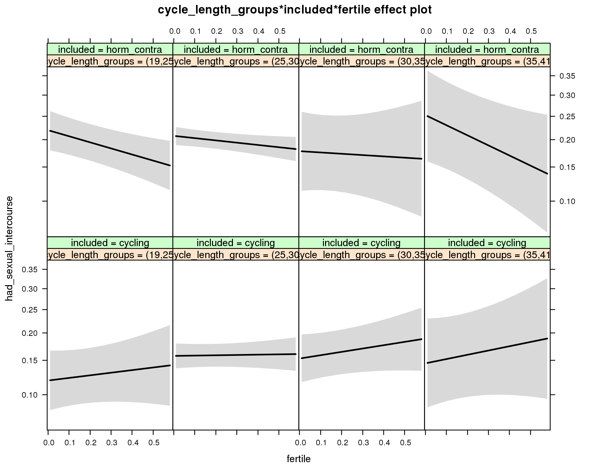
Generalized linear mixed model fit by maximum likelihood (Laplace Approximation) ['glmerMod']
Family: binomial ( probit )
Formula: had_sexual_intercourse ~ menstruation + fertile_mean + (1 | person) +
cycle_length_groups + included + fertile + menstruation:included +
cycle_length_groups:included + cycle_length_groups:fertile +
included:fertile + cycle_length_groups:included:fertile
Data: diary
AIC BIC logLik deviance df.resid
25713 25894 -12835 25669 26682
Scaled residuals:
Min 1Q Median 3Q Max
-2.635 -0.544 -0.376 -0.186 6.666
Random effects:
Groups Name Variance Std.Dev.
person (Intercept) 0.311 0.558
Number of obs: 26704, groups: person, 1054
Fixed effects:
Estimate Std. Error z value Pr(>|z|)
(Intercept) -1.1725 0.1217 -9.63 < 2e-16 ***
menstruationpre -0.0244 0.0470 -0.52 0.60430
menstruationyes -0.4134 0.0481 -8.60 < 2e-16 ***
fertile_mean 0.3933 0.3036 1.30 0.19517
cycle_length_groups(25,30] 0.1760 0.1180 1.49 0.13576
cycle_length_groups(30,35] 0.1571 0.1397 1.12 0.26070
cycle_length_groups(35,41] 0.1228 0.1961 0.63 0.53130
includedhorm_contra 0.4531 0.1330 3.41 0.00066 ***
fertile 0.1863 0.2639 0.71 0.48024
menstruationpre:includedhorm_contra -0.0634 0.0588 -1.08 0.28056
menstruationyes:includedhorm_contra -0.2039 0.0625 -3.26 0.00110 **
cycle_length_groups(25,30]:includedhorm_contra -0.2166 0.1420 -1.53 0.12711
cycle_length_groups(30,35]:includedhorm_contra -0.3070 0.2137 -1.44 0.15080
cycle_length_groups(35,41]:includedhorm_contra -0.0152 0.2666 -0.06 0.95450
cycle_length_groups(25,30]:fertile -0.1641 0.2801 -0.59 0.55802
cycle_length_groups(30,35]:fertile 0.0520 0.3261 0.16 0.87329
cycle_length_groups(35,41]:fertile 0.1192 0.4547 0.26 0.79328
includedhorm_contra:fertile -0.6209 0.3044 -2.04 0.04138 *
cycle_length_groups(25,30]:includedhorm_contra:fertile 0.4363 0.3247 1.34 0.17904
cycle_length_groups(30,35]:includedhorm_contra:fertile 0.2894 0.5064 0.57 0.56774
cycle_length_groups(35,41]:includedhorm_contra:fertile -0.4057 0.5826 -0.70 0.48627
---
Signif. codes: 0 '***' 0.001 '**' 0.01 '*' 0.05 '.' 0.1 ' ' 1
convergence code: 0
Model failed to converge with max|grad| = 0.190291 (tol = 0.001, component 1)
M_m7: Moderation by certainty about menstruation parameters
model %>%
test_moderator("certainty_menstruation", diary)| Df | AIC | BIC | logLik | deviance | Chisq | Chi Df | Pr(>Chisq) | |
|---|---|---|---|---|---|---|---|---|
| with_main | 12 | 25694 | 25793 | -12835 | 25670 | NA | NA | NA |
| with_mod | 14 | 25696 | 25811 | -12834 | 25668 | 2.236 | 2 | 0.327 |
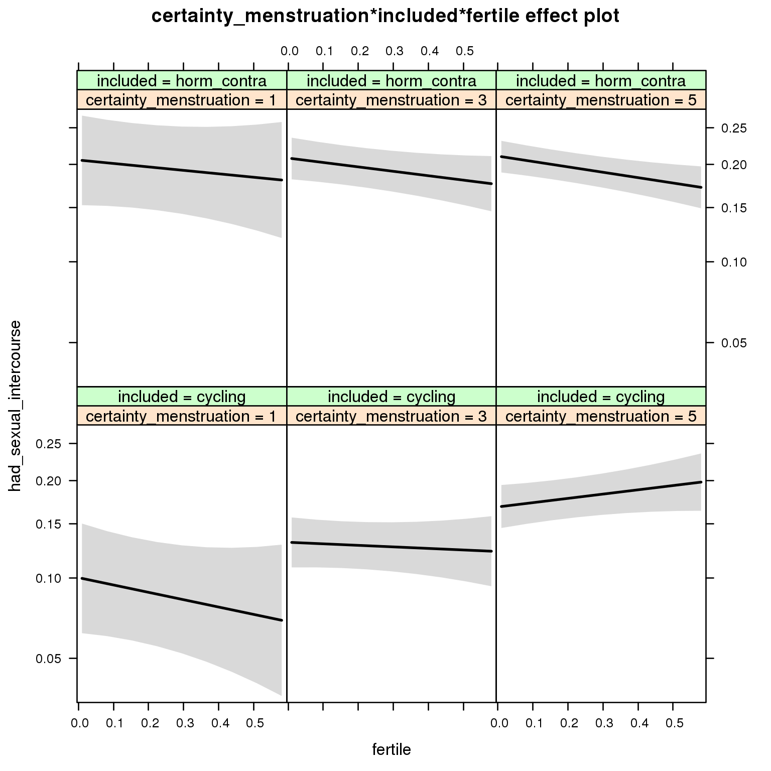
Generalized linear mixed model fit by maximum likelihood (Laplace Approximation) ['glmerMod']
Family: binomial ( probit )
Formula: had_sexual_intercourse ~ menstruation + fertile_mean + (1 | person) +
certainty_menstruation + included + fertile + menstruation:included +
certainty_menstruation:included + certainty_menstruation:fertile +
included:fertile + certainty_menstruation:included:fertile
Data: diary
AIC BIC logLik deviance df.resid
25696 25811 -12834 25668 26690
Scaled residuals:
Min 1Q Median 3Q Max
-2.723 -0.546 -0.375 -0.186 6.327
Random effects:
Groups Name Variance Std.Dev.
person (Intercept) 0.306 0.554
Number of obs: 26704, groups: person, 1054
Fixed effects:
Estimate Std. Error z value Pr(>|z|)
(Intercept) -1.3501 0.1710 -7.89 2.9e-15 ***
menstruationpre -0.0203 0.0470 -0.43 0.66600
menstruationyes -0.4080 0.0479 -8.52 < 2e-16 ***
fertile_mean 0.3730 0.3002 1.24 0.21397
certainty_menstruation 0.0799 0.0387 2.06 0.03908 *
includedhorm_contra 0.5843 0.2130 2.74 0.00607 **
fertile -0.4634 0.3955 -1.17 0.24123
menstruationpre:includedhorm_contra -0.0707 0.0587 -1.20 0.22886
menstruationyes:includedhorm_contra -0.2161 0.0622 -3.47 0.00052 ***
certainty_menstruation:includedhorm_contra -0.0754 0.0493 -1.53 0.12592
certainty_menstruation:fertile 0.1313 0.0912 1.44 0.14972
includedhorm_contra:fertile 0.3299 0.4900 0.67 0.50077
certainty_menstruation:includedhorm_contra:fertile -0.1532 0.1123 -1.36 0.17237
---
Signif. codes: 0 '***' 0.001 '**' 0.01 '*' 0.05 '.' 0.1 ' ' 1
convergence code: 0
Model failed to converge with max|grad| = 0.101611 (tol = 0.001, component 1)
M_m8: Moderation by cycle regularity
model %>%
test_moderator("cycle_regularity", diary)| Df | AIC | BIC | logLik | deviance | Chisq | Chi Df | Pr(>Chisq) | |
|---|---|---|---|---|---|---|---|---|
| with_main | 14 | 25702 | 25816 | -12837 | 25674 | NA | NA | NA |
| with_mod | 18 | 25709 | 25856 | -12836 | 25673 | 0.7208 | 4 | 0.9487 |
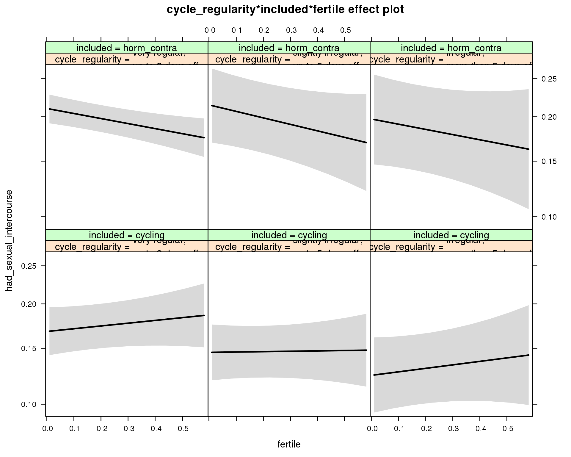
Generalized linear mixed model fit by maximum likelihood (Laplace Approximation) ['glmerMod']
Family: binomial ( probit )
Formula: had_sexual_intercourse ~ menstruation + fertile_mean + (1 | person) +
cycle_regularity + included + fertile + menstruation:included +
cycle_regularity:included + cycle_regularity:fertile + included:fertile +
cycle_regularity:included:fertile
Data: diary
AIC BIC logLik deviance df.resid
25709 25856 -12836 25673 26686
Scaled residuals:
Min 1Q Median 3Q Max
-2.675 -0.545 -0.376 -0.186 6.403
Random effects:
Groups Name Variance Std.Dev.
person (Intercept) 0.309 0.556
Number of obs: 26704, groups: person, 1054
Fixed effects:
Estimate Std. Error z value
(Intercept) -0.9547 0.0756 -12.63
menstruationpre -0.0250 0.0470 -0.53
menstruationyes -0.4130 0.0478 -8.63
fertile_mean 0.3964 0.3004 1.32
cycle_regularityslightly irregular,\nup to 5 days off -0.0918 0.0818 -1.12
cycle_regularityirregular,\nmore than 5 days off -0.1925 0.0996 -1.93
includedhorm_contra 0.2053 0.0675 3.04
fertile 0.1216 0.1281 0.95
menstruationpre:includedhorm_contra -0.0662 0.0588 -1.13
menstruationyes:includedhorm_contra -0.2112 0.0622 -3.39
cycle_regularityslightly irregular,\nup to 5 days off:includedhorm_contra 0.1074 0.1211 0.89
cycle_regularityirregular,\nmore than 5 days off:includedhorm_contra 0.1462 0.1455 1.00
cycle_regularityslightly irregular,\nup to 5 days off:fertile -0.1051 0.1799 -0.58
cycle_regularityirregular,\nmore than 5 days off:fertile 0.0316 0.2260 0.14
includedhorm_contra:fertile -0.3430 0.1484 -2.31
cycle_regularityslightly irregular,\nup to 5 days off:includedhorm_contra:fertile 0.0413 0.2628 0.16
cycle_regularityirregular,\nmore than 5 days off:includedhorm_contra:fertile -0.0386 0.3238 -0.12
Pr(>|z|)
(Intercept) < 2e-16 ***
menstruationpre 0.59470
menstruationyes < 2e-16 ***
fertile_mean 0.18696
cycle_regularityslightly irregular,\nup to 5 days off 0.26190
cycle_regularityirregular,\nmore than 5 days off 0.05326 .
includedhorm_contra 0.00236 **
fertile 0.34239
menstruationpre:includedhorm_contra 0.25976
menstruationyes:includedhorm_contra 0.00069 ***
cycle_regularityslightly irregular,\nup to 5 days off:includedhorm_contra 0.37535
cycle_regularityirregular,\nmore than 5 days off:includedhorm_contra 0.31496
cycle_regularityslightly irregular,\nup to 5 days off:fertile 0.55928
cycle_regularityirregular,\nmore than 5 days off:fertile 0.88864
includedhorm_contra:fertile 0.02084 *
cycle_regularityslightly irregular,\nup to 5 days off:includedhorm_contra:fertile 0.87502
cycle_regularityirregular,\nmore than 5 days off:includedhorm_contra:fertile 0.90511
---
Signif. codes: 0 '***' 0.001 '**' 0.01 '*' 0.05 '.' 0.1 ' ' 1
convergence code: 0
Model failed to converge with max|grad| = 0.0642138 (tol = 0.001, component 1)
M_m9: Moderation by cohabitation status
model %>%
test_moderator("cohabitation", diary)| Df | AIC | BIC | logLik | deviance | Chisq | Chi Df | Pr(>Chisq) | |
|---|---|---|---|---|---|---|---|---|
| with_main | 14 | 25658 | 25772 | -12815 | 25630 | NA | NA | NA |
| with_mod | 18 | 25655 | 25803 | -12810 | 25619 | 10.41 | 4 | 0.034 |
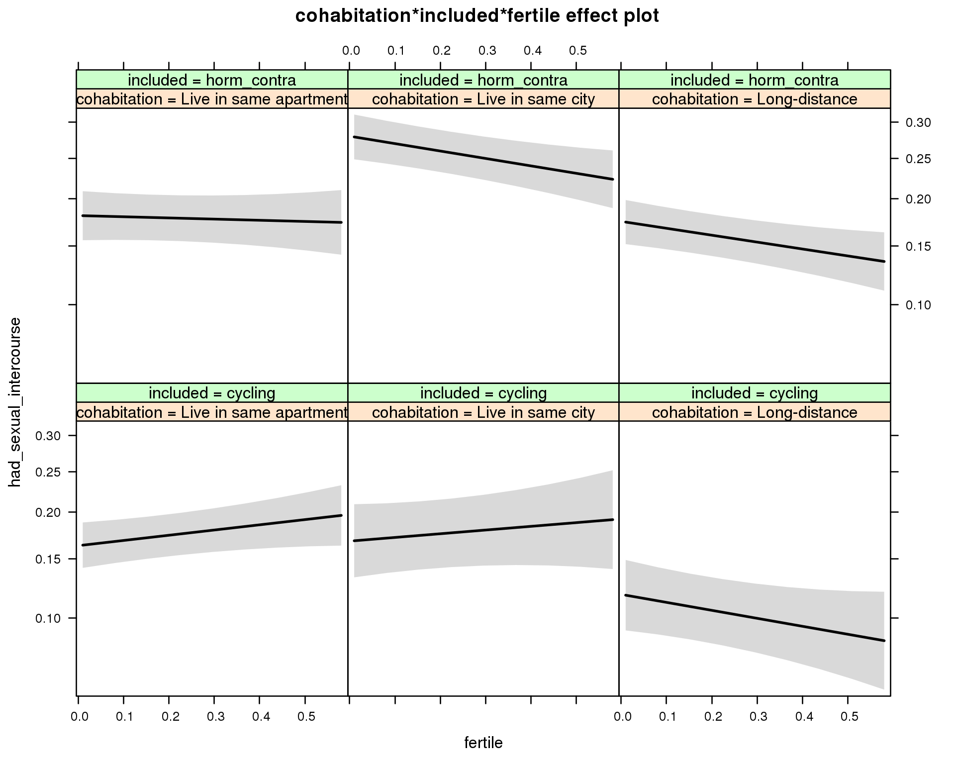
Generalized linear mixed model fit by maximum likelihood (Laplace Approximation) ['glmerMod']
Family: binomial ( probit )
Formula: had_sexual_intercourse ~ menstruation + fertile_mean + (1 | person) +
cohabitation + included + fertile + menstruation:included +
cohabitation:included + cohabitation:fertile + included:fertile + cohabitation:included:fertile
Data: diary
AIC BIC logLik deviance df.resid
25655 25803 -12810 25619 26686
Scaled residuals:
Min 1Q Median 3Q Max
-2.682 -0.545 -0.375 -0.181 6.113
Random effects:
Groups Name Variance Std.Dev.
person (Intercept) 0.29 0.538
Number of obs: 26704, groups: person, 1054
Fixed effects:
Estimate Std. Error z value Pr(>|z|)
(Intercept) -0.9638 0.0720 -13.39 < 2e-16 ***
menstruationpre -0.0239 0.0469 -0.51 0.61009
menstruationyes -0.4107 0.0478 -8.60 < 2e-16 ***
fertile_mean 0.3345 0.2945 1.14 0.25608
cohabitationLive in same city 0.0188 0.0910 0.21 0.83643
cohabitationLong-distance -0.2022 0.0885 -2.29 0.02229 *
includedhorm_contra 0.1199 0.0749 1.60 0.10952
fertile 0.2164 0.1154 1.88 0.06074 .
menstruationpre:includedhorm_contra -0.0698 0.0587 -1.19 0.23449
menstruationyes:includedhorm_contra -0.2145 0.0622 -3.45 0.00056 ***
cohabitationLive in same city:includedhorm_contra 0.3105 0.1152 2.70 0.00703 **
cohabitationLong-distance:includedhorm_contra 0.1780 0.1128 1.58 0.11448
cohabitationLive in same city:fertile -0.0627 0.2086 -0.30 0.76367
cohabitationLong-distance:fertile -0.5474 0.2087 -2.62 0.00871 **
includedhorm_contra:fertile -0.2651 0.1670 -1.59 0.11246
cohabitationLive in same city:includedhorm_contra:fertile -0.1969 0.2584 -0.76 0.44621
cohabitationLong-distance:includedhorm_contra:fertile 0.3094 0.2595 1.19 0.23311
---
Signif. codes: 0 '***' 0.001 '**' 0.01 '*' 0.05 '.' 0.1 ' ' 1
convergence code: 0
Model failed to converge with max|grad| = 0.0734515 (tol = 0.001, component 1)
M_m10: Moderation by relationship status
model %>%
test_moderator("relationship_status_clean", diary)| Df | AIC | BIC | logLik | deviance | Chisq | Chi Df | Pr(>Chisq) | |
|---|---|---|---|---|---|---|---|---|
| with_main | 14 | 25695 | 25810 | -12834 | 25667 | NA | NA | NA |
| with_mod | 18 | 25697 | 25844 | -12830 | 25661 | 6.193 | 4 | 0.1852 |
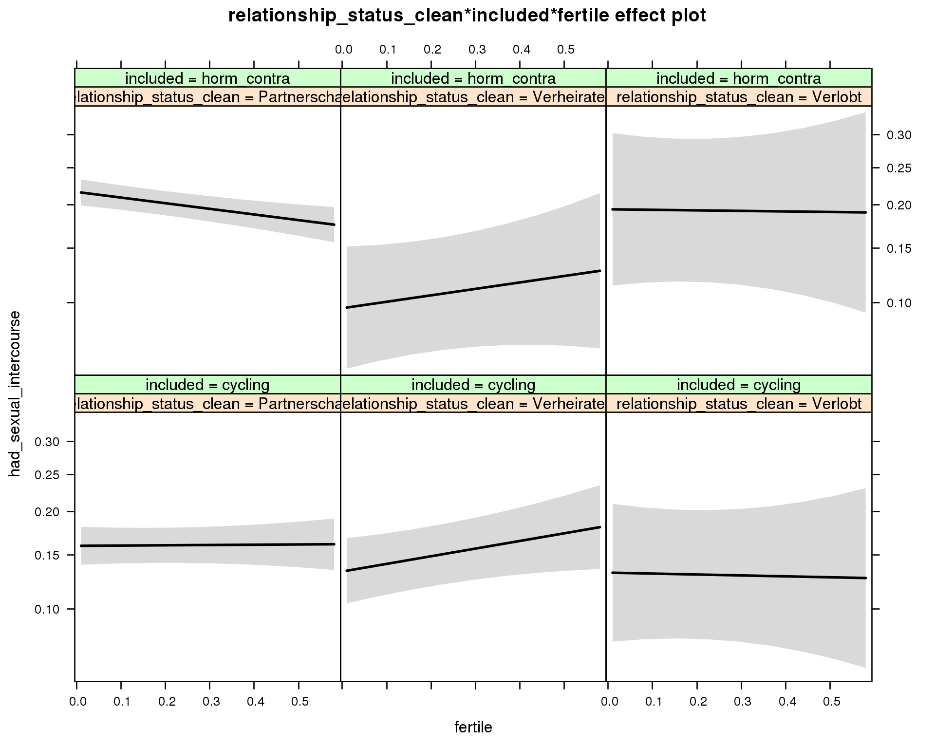
Generalized linear mixed model fit by maximum likelihood (Laplace Approximation) ['glmerMod']
Family: binomial ( probit )
Formula: had_sexual_intercourse ~ menstruation + fertile_mean + (1 | person) +
relationship_status_clean + included + fertile + menstruation:included +
relationship_status_clean:included + relationship_status_clean:fertile +
included:fertile + relationship_status_clean:included:fertile
Data: diary
AIC BIC logLik deviance df.resid
25697 25844 -12830 25661 26686
Scaled residuals:
Min 1Q Median 3Q Max
-2.562 -0.546 -0.376 -0.185 6.271
Random effects:
Groups Name Variance Std.Dev.
person (Intercept) 0.306 0.553
Number of obs: 26704, groups: person, 1054
Fixed effects:
Estimate Std. Error z value Pr(>|z|)
(Intercept) -0.9892 0.0682 -14.49 < 2e-16 ***
menstruationpre -0.0259 0.0470 -0.55 0.58195
menstruationyes -0.4140 0.0478 -8.66 < 2e-16 ***
fertile_mean 0.4020 0.2988 1.35 0.17849
relationship_status_cleanVerheiratet -0.1158 0.0865 -1.34 0.18067
relationship_status_cleanVerlobt -0.1210 0.1652 -0.73 0.46394
includedhorm_contra 0.2617 0.0585 4.47 0.0000077 ***
fertile 0.0124 0.1080 0.11 0.90864
menstruationpre:includedhorm_contra -0.0660 0.0588 -1.12 0.26102
menstruationyes:includedhorm_contra -0.2115 0.0622 -3.40 0.00068 ***
relationship_status_cleanVerheiratet:includedhorm_contra -0.4084 0.1686 -2.42 0.01540 *
relationship_status_cleanVerlobt:includedhorm_contra 0.0428 0.2438 0.18 0.86068
relationship_status_cleanVerheiratet:fertile 0.3323 0.1912 1.74 0.08225 .
relationship_status_cleanVerlobt:fertile -0.0542 0.3703 -0.15 0.88371
includedhorm_contra:fertile -0.2667 0.1290 -2.07 0.03872 *
relationship_status_cleanVerheiratet:includedhorm_contra:fertile 0.2126 0.3747 0.57 0.57052
relationship_status_cleanVerlobt:includedhorm_contra:fertile 0.2841 0.5489 0.52 0.60467
---
Signif. codes: 0 '***' 0.001 '**' 0.01 '*' 0.05 '.' 0.1 ' ' 1
convergence code: 0
Model failed to converge with max|grad| = 0.0763988 (tol = 0.001, component 1)
Specific robustness analyses for sexual intercourse
xtabs(~ spent_night_with_partner + had_sexual_intercourse, data = diary %>% filter(!is.na(fertile), !is.na(included)))## had_sexual_intercourse
## spent_night_with_partner 0 1
## 0 11719 681
## 1 9236 5068possible_nights = diary %>% filter(spent_night_with_partner == 1)
m1_night_with_partner = glmer(had_sexual_intercourse ~ included * (menstruation + fertile) + fertile_mean + ( 1 | person), data = possible_nights, family = binomial(link = "probit"))
m1_night_with_partner %>%
print_summary() %>%
plot_all_effects()##
##
## ```
## Generalized linear mixed model fit by maximum likelihood (Laplace Approximation) ['glmerMod']
## Family: binomial ( probit )
## Formula: had_sexual_intercourse ~ included * (menstruation + fertile) + fertile_mean + (1 | person)
## Data: possible_nights
##
## AIC BIC logLik deviance df.resid
## 15903 15979 -7942 15883 14294
##
## Scaled residuals:
## Min 1Q Median 3Q Max
## -4.237 -0.619 -0.347 0.684 6.647
##
## Random effects:
## Groups Name Variance Std.Dev.
## person (Intercept) 0.656 0.81
## Number of obs: 14304, groups: person, 972
##
## Fixed effects:
## Estimate Std. Error z value Pr(>|z|)
## (Intercept) -0.5439 0.0920 -5.92 3.3e-09 ***
## includedhorm_contra 0.5527 0.0759 7.28 3.3e-13 ***
## menstruationpre -0.0128 0.0596 -0.21 0.83006
## menstruationyes -0.5247 0.0597 -8.79 < 2e-16 ***
## fertile 0.1791 0.1196 1.50 0.13417
## fertile_mean 0.1773 0.4278 0.41 0.67849
## includedhorm_contra:menstruationpre -0.0582 0.0777 -0.75 0.45371
## includedhorm_contra:menstruationyes -0.2889 0.0805 -3.59 0.00033 ***
## includedhorm_contra:fertile -0.3243 0.1542 -2.10 0.03545 *
## ---
## Signif. codes: 0 '***' 0.001 '**' 0.01 '*' 0.05 '.' 0.1 ' ' 1
##
## Correlation of Fixed Effects:
## (Intr) incld_ mnstrtnp mnstrtny fertil frtl_m inclddhrm_cntr:mnstrtnp
## inclddhrm_c -0.475
## menstrutnpr -0.253 0.317
## menstrutnys -0.220 0.275 0.370
## fertile -0.245 0.386 0.476 0.369
## fertile_men -0.765 -0.036 -0.011 -0.010 -0.091
## inclddhrm_cntr:mnstrtnp 0.204 -0.400 -0.767 -0.284 -0.364 -0.004
## inclddhrm_cntr:mnstrtny 0.173 -0.343 -0.274 -0.740 -0.273 -0.004 0.350
## inclddhrm_cntr:f 0.247 -0.493 -0.368 -0.285 -0.769 -0.003 0.468
## inclddhrm_cntr:mnstrtny
## inclddhrm_c
## menstrutnpr
## menstrutnys
## fertile
## fertile_men
## inclddhrm_cntr:mnstrtnp
## inclddhrm_cntr:mnstrtny
## inclddhrm_cntr:f 0.357
## convergence code: 0
## Model failed to converge with max|grad| = 0.00964787 (tol = 0.001, component 1)
##
##
## ```
In-pair desire predicts having sex.
summary(glmer(had_sexual_intercourse ~ in_pair_desire + included + menstruation + ( 1 | person), data = diary, family = binomial(link = "probit")))## Generalized linear mixed model fit by maximum likelihood (Laplace Approximation) ['glmerMod']
## Family: binomial ( probit )
## Formula: had_sexual_intercourse ~ in_pair_desire + included + menstruation + (1 | person)
## Data: diary
##
## AIC BIC logLik deviance df.resid
## 18937 18987 -9463 18925 27795
##
## Scaled residuals:
## Min 1Q Median 3Q Max
## -6.61 -0.37 -0.12 -0.01 126.16
##
## Random effects:
## Groups Name Variance Std.Dev.
## person (Intercept) 0.624 0.79
## Number of obs: 27801, groups: person, 1054
##
## Fixed effects:
## Estimate Std. Error z value Pr(>|z|)
## (Intercept) -4.7544 0.0775 -61.4 <2e-16 ***
## in_pair_desire 0.9464 0.0139 67.9 <2e-16 ***
## includedhorm_contra 0.0978 0.0590 1.7 0.097 .
## menstruationpre -0.0218 0.0306 -0.7 0.476
## menstruationyes -0.5436 0.0345 -15.8 <2e-16 ***
## ---
## Signif. codes: 0 '***' 0.001 '**' 0.01 '*' 0.05 '.' 0.1 ' ' 1
##
## Correlation of Fixed Effects:
## (Intr) in_pr_ incld_ mnstrtnp
## in_pair_dsr -0.793
## inclddhrm_c -0.474 0.001
## menstrutnpr -0.090 0.011 0.008
## menstrutnys -0.029 -0.059 0.013 0.201Ovulatory but menstrual changes in sex are mediated by in-pair desire.
summary(glmer(had_sexual_intercourse ~ in_pair_desire + included * (menstruation + fertile) + fertile_mean + ( 1 | person), data = diary, family = binomial(link = "probit")))## Generalized linear mixed model fit by maximum likelihood (Laplace Approximation) ['glmerMod']
## Family: binomial ( probit )
## Formula: had_sexual_intercourse ~ in_pair_desire + included * (menstruation +
## fertile) + fertile_mean + (1 | person)
## Data: diary
##
## AIC BIC logLik deviance df.resid
## 18026 18116 -9002 18004 26669
##
## Scaled residuals:
## Min 1Q Median 3Q Max
## -6.27 -0.36 -0.12 -0.01 93.86
##
## Random effects:
## Groups Name Variance Std.Dev.
## person (Intercept) 0.614 0.784
## Number of obs: 26680, groups: person, 1054
##
## Fixed effects:
## Estimate Std. Error z value Pr(>|z|)
## (Intercept) -4.8912 0.1085 -45.1 < 2e-16 ***
## in_pair_desire 0.9526 0.0144 66.1 < 2e-16 ***
## includedhorm_contra 0.1477 0.0707 2.1 0.037 *
## menstruationpre 0.0190 0.0577 0.3 0.743
## menstruationyes -0.3778 0.0584 -6.5 0.000000000097 ***
## fertile -0.1171 0.1159 -1.0 0.312
## fertile_mean 0.5264 0.4067 1.3 0.196
## includedhorm_contra:menstruationpre -0.1057 0.0722 -1.5 0.143
## includedhorm_contra:menstruationyes -0.3521 0.0760 -4.6 0.000003637977 ***
## includedhorm_contra:fertile -0.0248 0.1436 -0.2 0.863
## ---
## Signif. codes: 0 '***' 0.001 '**' 0.01 '*' 0.05 '.' 0.1 ' ' 1
##
## Correlation of Fixed Effects:
## (Intr) in_pr_ incld_ mnstrtnp mnstrtny fertil frtl_m inclddhrm_cntr:mnstrtnp
## in_pair_dsr -0.591
## inclddhrm_c -0.384 -0.003
## menstrutnpr -0.216 0.013 0.324
## menstrutnys -0.172 -0.010 0.280 0.356
## fertile -0.190 -0.022 0.403 0.467 0.355
## fertile_men -0.624 0.010 -0.040 -0.005 -0.007 -0.092
## inclddhrm_cntr:mnstrtnp 0.180 -0.012 -0.395 -0.800 -0.285 -0.373 -0.007
## inclddhrm_cntr:mnstrtny 0.168 -0.040 -0.330 -0.274 -0.767 -0.271 -0.006 0.337
## inclddhrm_cntr:f 0.191 0.021 -0.495 -0.377 -0.286 -0.802 0.011 0.464
## inclddhrm_cntr:mnstrtny
## in_pair_dsr
## inclddhrm_c
## menstrutnpr
## menstrutnys
## fertile
## fertile_men
## inclddhrm_cntr:mnstrtnp
## inclddhrm_cntr:mnstrtny
## inclddhrm_cntr:f 0.341
## convergence code: 0
## Model failed to converge with max|grad| = 0.563778 (tol = 0.001, component 1)Partner initiated sex
model_summaries$partner_initiated_sexual_intercourseModel summary
Model summary
model %>%
print_summary()Generalized linear mixed model fit by maximum likelihood (Laplace Approximation) ['glmerMod']
Family: binomial ( probit )
Formula: partner_initiated_sexual_intercourse ~ included * (menstruation +
fertile) + fertile_mean + (1 | person)
Data: diary
AIC BIC logLik deviance df.resid
7646 7713 -3813 7626 5738
Scaled residuals:
Min 1Q Median 3Q Max
-1.740 -1.111 0.659 0.779 1.288
Random effects:
Groups Name Variance Std.Dev.
person (Intercept) 0.0914 0.302
Number of obs: 5748, groups: person, 859
Fixed effects:
Estimate Std. Error z value Pr(>|z|)
(Intercept) 0.1442 0.0821 1.76 0.0790 .
includedhorm_contra 0.1055 0.0730 1.45 0.1484
menstruationpre 0.0386 0.0879 0.44 0.6608
menstruationyes 0.0657 0.0959 0.69 0.4929
fertile -0.2666 0.1761 -1.51 0.1301
fertile_mean 0.6074 0.3621 1.68 0.0934 .
includedhorm_contra:menstruationpre -0.1141 0.1088 -1.05 0.2942
includedhorm_contra:menstruationyes -0.3503 0.1263 -2.77 0.0055 **
includedhorm_contra:fertile 0.3013 0.2161 1.39 0.1634
---
Signif. codes: 0 '***' 0.001 '**' 0.01 '*' 0.05 '.' 0.1 ' ' 1
Correlation of Fixed Effects:
(Intr) incld_ mnstrtnp mnstrtny fertil frtl_m inclddhrm_cntr:mnstrtnp
inclddhrm_c -0.558
menstrutnpr -0.423 0.481
menstrutnys -0.321 0.366 0.304
fertile -0.426 0.597 0.471 0.308
fertile_men -0.687 -0.047 -0.006 -0.006 -0.145
inclddhrm_cntr:mnstrtnp 0.351 -0.580 -0.808 -0.246 -0.377 -0.011
inclddhrm_cntr:mnstrtny 0.243 -0.422 -0.231 -0.759 -0.233 0.004 0.284
inclddhrm_cntr:f 0.423 -0.727 -0.383 -0.251 -0.799 0.008 0.466
inclddhrm_cntr:mnstrtny
inclddhrm_c
menstrutnpr
menstrutnys
fertile
fertile_men
inclddhrm_cntr:mnstrtnp
inclddhrm_cntr:mnstrtny
inclddhrm_cntr:f 0.295
Effect size standardised by residual variance (\(\frac{b}{ SD_{residual} }\)): -0.27 [-0.61;0.08].
Marginal effect plots
model %>%
plot_all_effects()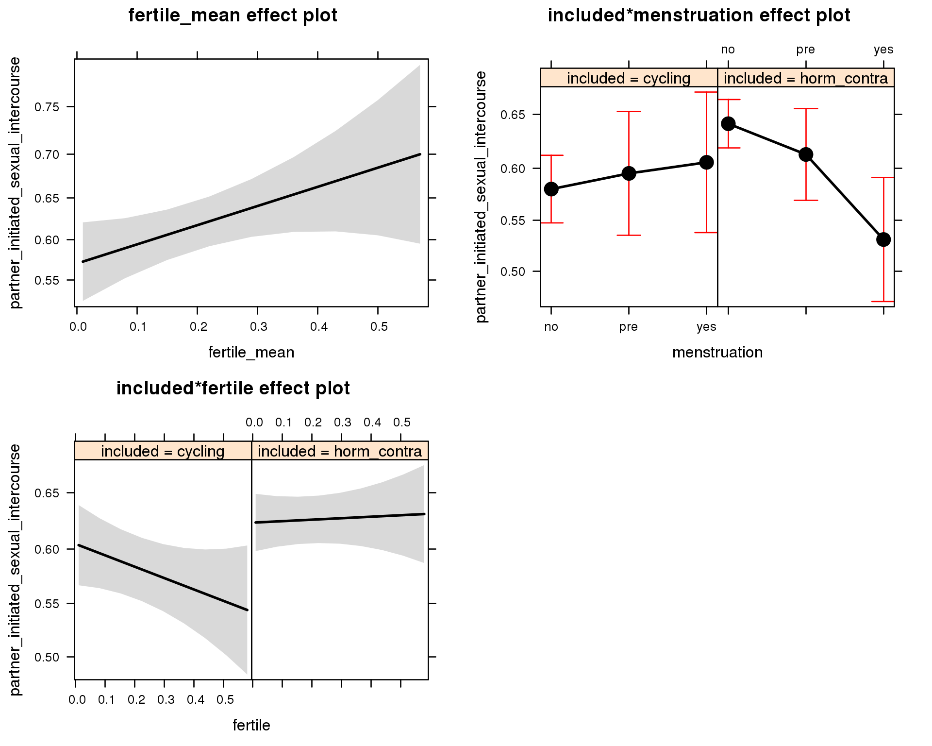
Outcome distribution
model %>%
plot_outcome(diary) + xlab(outcome_label)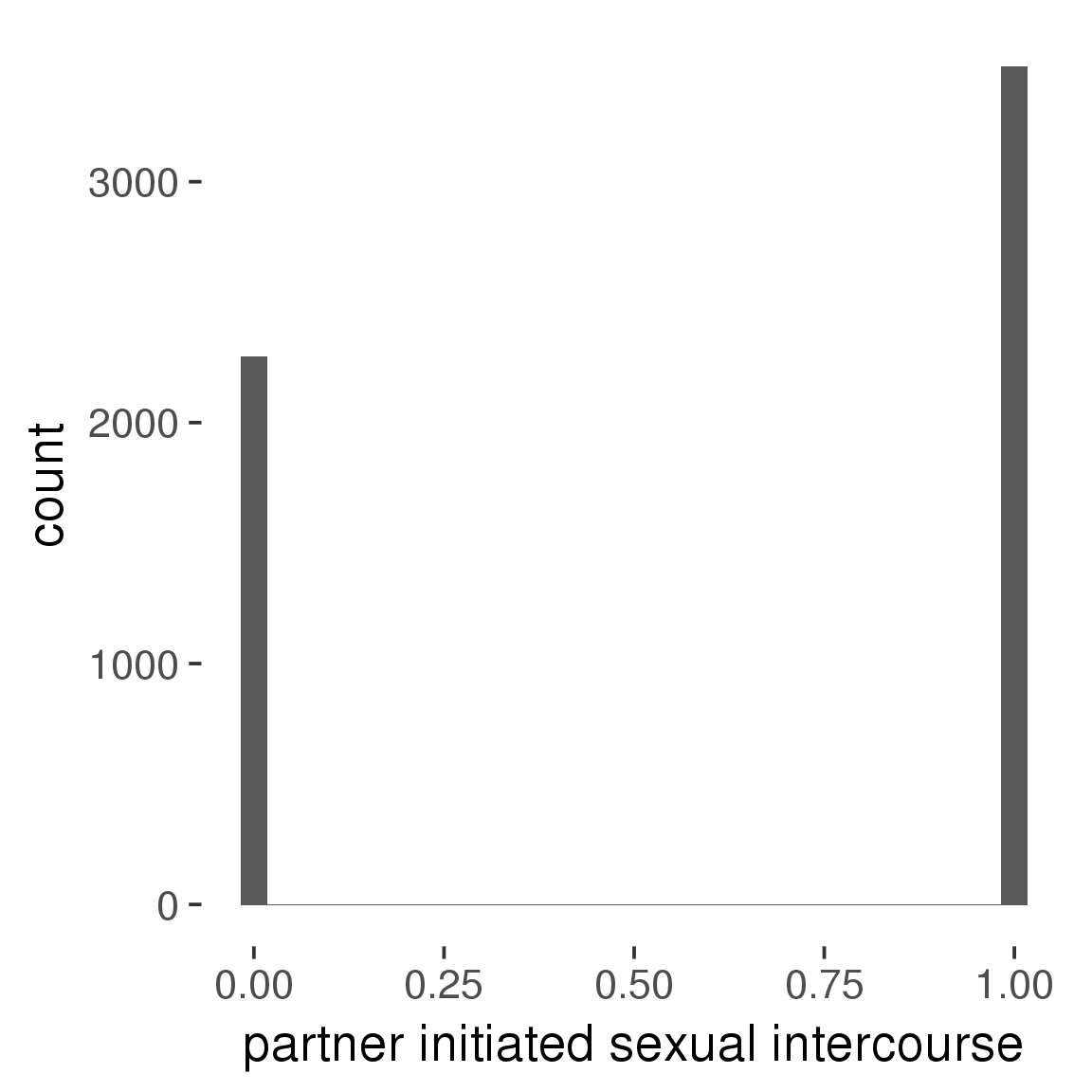
Diagnostics
model %>%
print_diagnostics()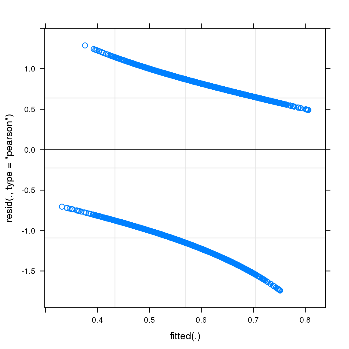
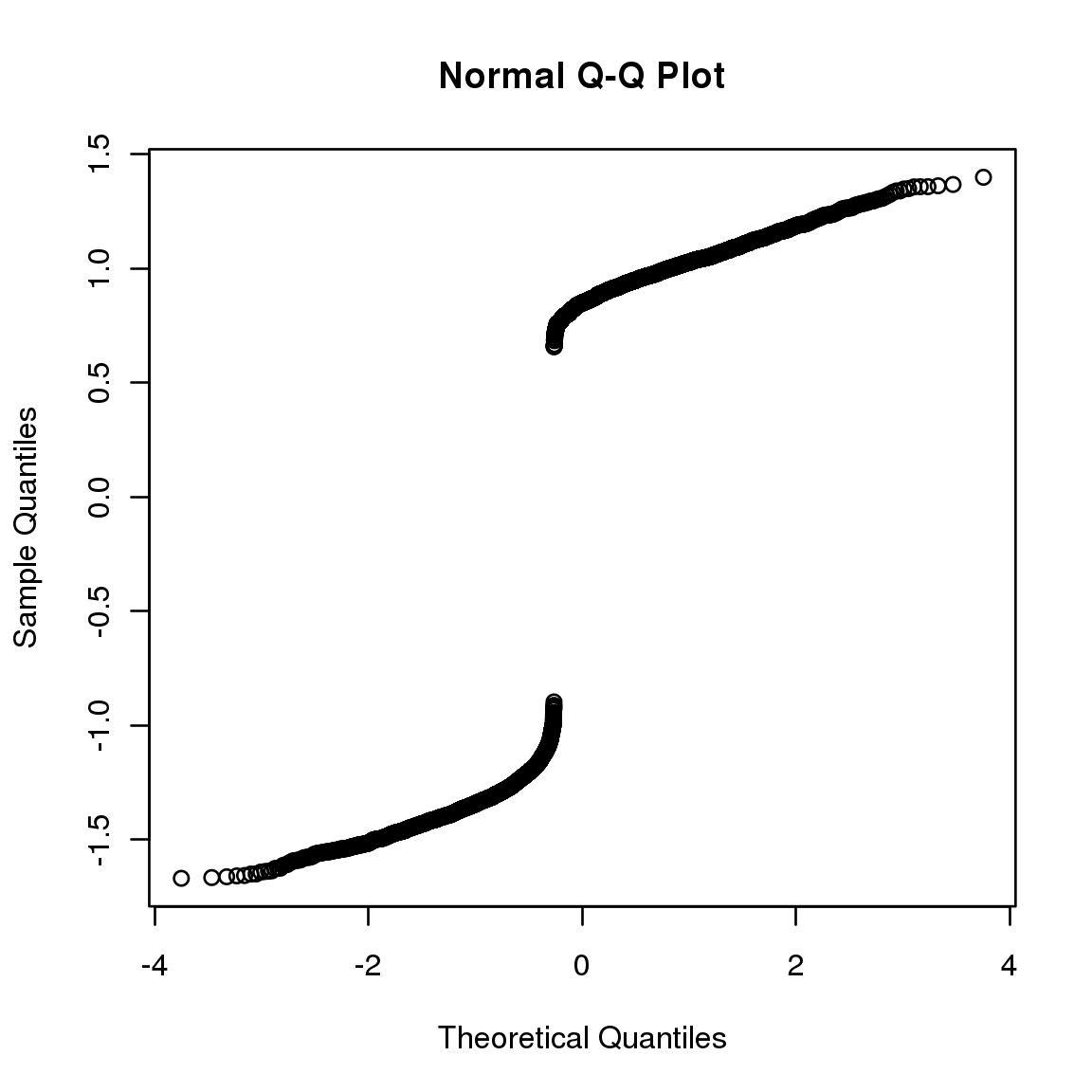
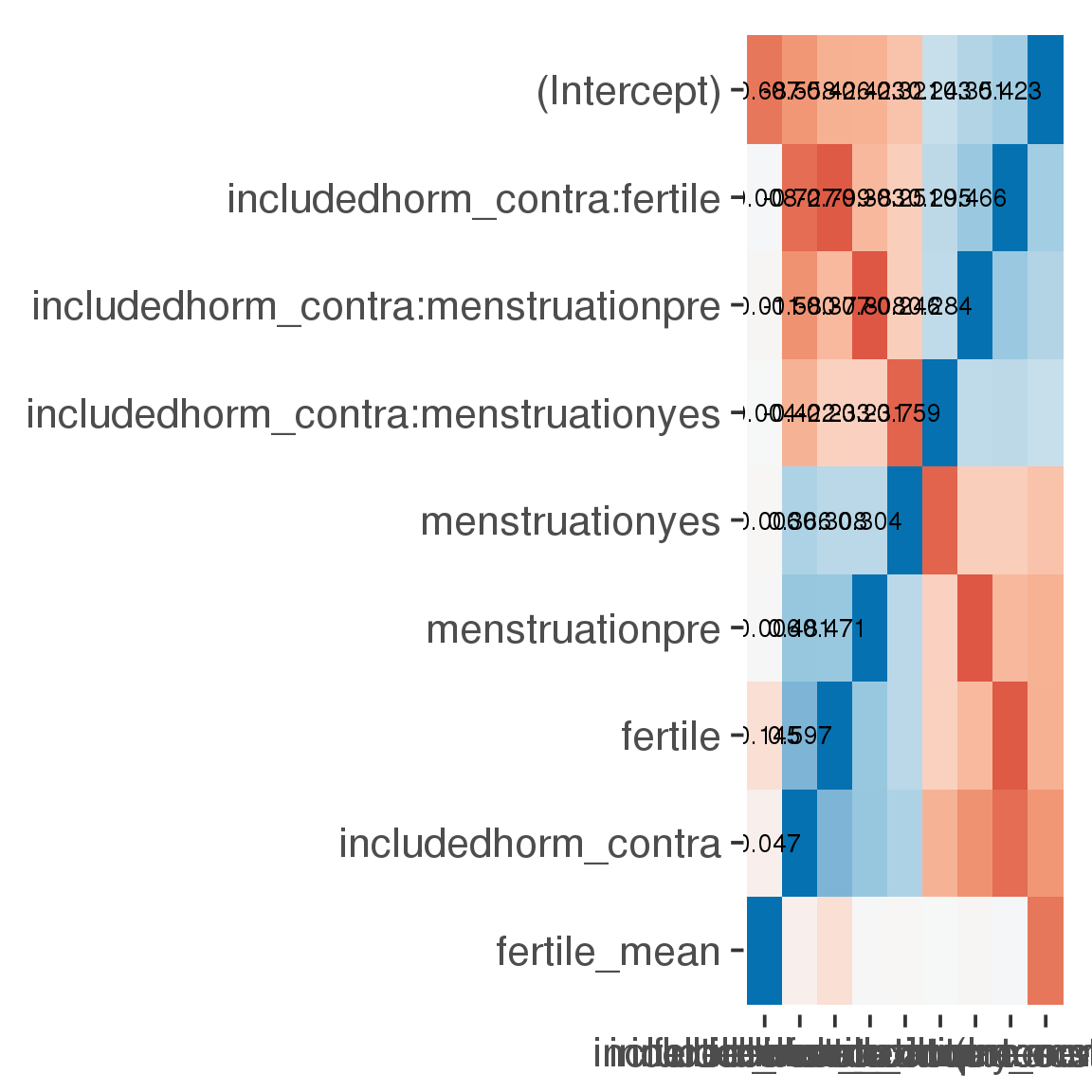
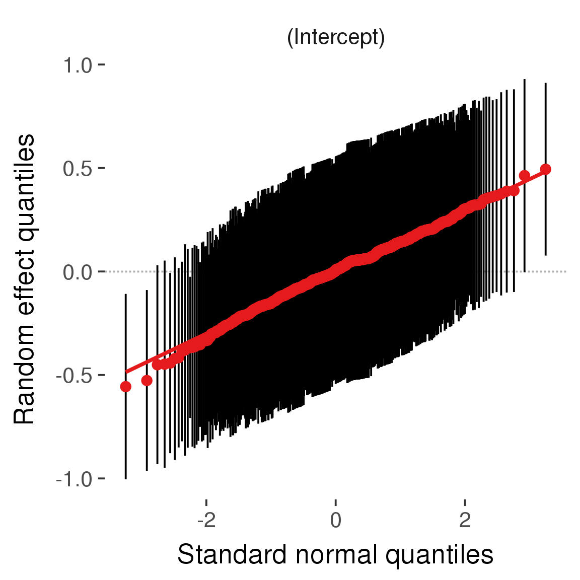
Curves
Here, we continuously plot the outcome over the course of the cycle. Because cycle lengths vary, we subset the data to cycles in a certain range. If the red curve traces the pink curve, our predictor accurately maps the relationship between fertile window probability and the outcome.
Cycle lengths from 21 to 36
Backward-counted
model %>%
plot_curve(diary %>% filter(minimum_cycle_length_diary <= 36, minimum_cycle_length_diary > 20) %>% mutate(fertile=prc_stirn_b))outcome = names(model@frame)[1]
outcome_label = recode(str_replace_all(str_replace_all(str_replace_all(outcome, "_", " "), " pair", "-pair"), " 1", ""),
"desirability 1" = "self-perceived desirability",
"NARQ admiration" = "narcissistic admiration",
"NARQ rivalry" = "narcissistic rivalry",
"extra-pair" = "extra-pair desire & behaviour",
"had sexual intercourse" = "sexual intercourse")
library(ggplot2)
# form a subset and run the model without the hormonal contraception and the fertility predictors
tmp = diary %>%
filter(!is.na(fertile), !is.na(included),
RCD > -1 * minimum_cycle_length_diary, RCD > -40)
new_form = update.formula(formula(model), new = . ~ . - fertile * included)
tmp$residuals = residuals(update(model, new_form, data = tmp , na.action = na.exclude))
tmp = tmp %>%
filter(!is.na(RCD), !is.na(residuals))
rcd_min = min(tmp$RCD)
tmp$real = FALSE
tmp_before = tmp
tmp_before$RCD = tmp_before$RCD + min(tmp$RCD) - 1
tmp_after = tmp
tmp_after$RCD = tmp_after$RCD - min(tmp$RCD) + 1
tmp$real = TRUE
tmp = bind_rows(tmp_before %>% filter(RCD > rcd_min - 11), tmp, tmp_after %>% filter(RCD < 11))GAM smooth on residuals
Here, we partialled out menstruation and individual random effects, then superimposed estimated probability of being in the fertile window scaled to the range of the estimated means. To address the periodicity of the cycle, we prepended and appended ten days of the timeseries to the end and the beginning of the timeseries. We then estimated the GAM and cut off the appended subsets before plotting.
tryCatch({
trend_plot = ggplot(tmp,aes(x = RCD, y = residuals, colour = included)) +
stat_smooth(geom = 'smooth',size = 0.8, fill = "#9ECAE1", method = 'gam', formula = y ~ s(x))
}, error = function(e){cat_message(e, "danger")})
tryCatch({
trend_data = ggplot_build(trend_plot)$data[[1]]
}, error = function(e){cat_message(e, "danger")})
trend_data$RCD = round(trend_data$x)
trend_data = left_join(trend_data, tmp %>% select(real, RCD,fertile) %>% unique(), by = "RCD")
trend_data %>%
filter(real == TRUE) %>%
mutate(superimposed = ( ( (fertile - 0.01)/0.58) * (max(y)-min(y) ) ) + min(y) ) ->
trend_data
ggplot(trend_data) +
geom_ribbon(aes(x = x, ymin = ymin, ymax = ymax, fill = factor(group)), alpha = 0.2) +
geom_line(aes(x = x, y = y, colour = factor(group)), size = 0.8, stat = "identity") +
scale_x_continuous(caption_x) +
geom_line(aes(x = x, y = superimposed), color = "#a83fbf", size = 1, linetype = 'dashed') +
annotate("text",x = mean(trend_data$x), y = max(trend_data$superimposed,na.rm=T) + 0.1, label = 'superimposed fertility peak', color = "#a83fbf") +
scale_y_continuous(outcome_label) +
ggtitle("GAM smooth, residuals") +
scale_color_manual("Contraception status",values = c("2"="black","1"= "red"), labels = c("2"="hormonally\ncontracepting","1"="cycling"), guide = F) +
scale_fill_manual("Contraception status",values = c("2"="black","1"= "red"), labels = c("2"="hormonally\ncontracepting","1"="cycling"), guide = F)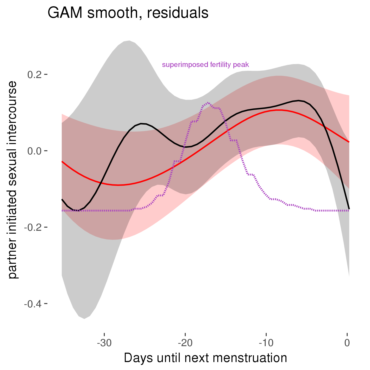
GAM smooth on raw data
As before, but without partialling anything out.
tryCatch({
trend_plot = ggplot(tmp,aes_string(x = "RCD", y = outcome, colour = "included")) +
stat_smooth(geom = 'smooth',size = 0.8, fill = "#9ECAE1", method = 'gam', formula = y ~ s(x))
}, error = function(e){cat_message(e, "danger")})
tryCatch({
trend_data = ggplot_build(trend_plot)$data[[1]]
}, error = function(e){cat_message(e, "danger")})
trend_data$RCD = round(trend_data$x)
trend_data = left_join(trend_data, tmp %>% select(real, RCD,fertile) %>% unique(), by = "RCD")
trend_data %>%
filter(real == TRUE) %>%
mutate(superimposed = ( ( (fertile - 0.01)/0.58) * (max(y)-min(y) ) ) + min(y) ) ->
trend_data
plot1b = ggplot(trend_data) +
geom_ribbon(aes(x = x, ymin = ymin, ymax = ymax, fill = factor(group)), alpha = 0.2) +
geom_line(aes(x = x, y = y, colour = factor(group)), size = 0.8, stat = "identity") +
scale_x_continuous(caption_x) +
geom_line(aes(x = x, y = superimposed), color = "#a83fbf", size = 1, linetype = 'dashed') +
annotate("text",x = mean(trend_data$x), y = max(trend_data$superimposed,na.rm=T) + 0.1, label = 'superimposed fertility peak', color = "#a83fbf") +
scale_y_continuous(outcome_label) +
ggtitle("GAM smooth, raw data") +
scale_color_manual("Contraception status",values = c("2"="black","1"= "red"), labels = c("2"="hormonally\ncontracepting","1"="cycling"), guide = F) +
scale_fill_manual("Contraception status",values = c("2"="black","1"= "red"), labels = c("2"="hormonally\ncontracepting","1"="cycling"), guide = F)
suppressWarnings(print(plot1b))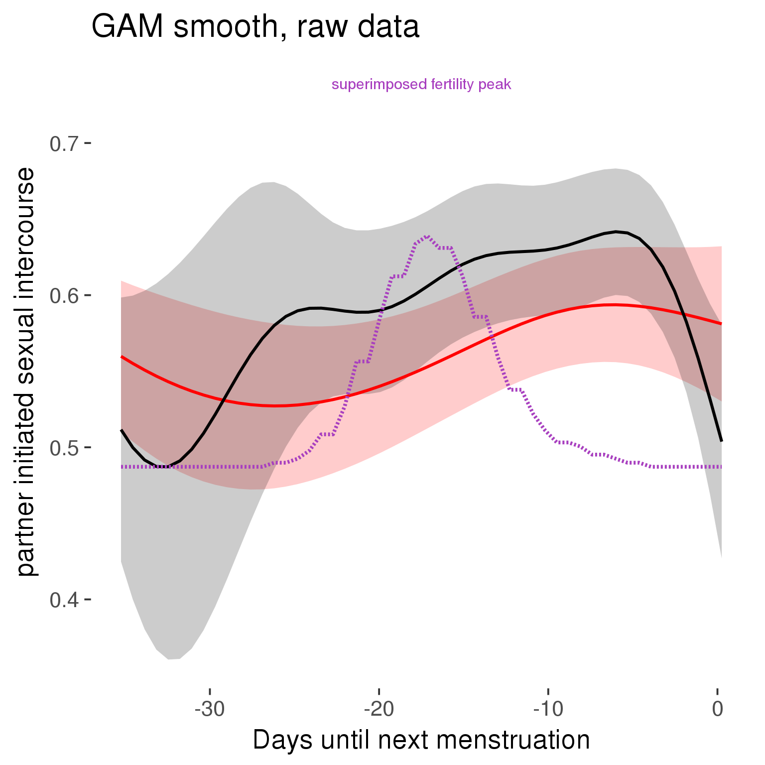
Means and standard errors over raw data
Nothing partialled out, just straight means with bootstrapped confidence intervals.
tryCatch({
trend_plot = ggplot(tmp,aes_string(x = "RCD", y = outcome, colour = "included")) +
geom_pointrange(size = 0.8, stat = 'summary', fun.data = "mean_cl_boot")
}, error = function(e){cat_message(e, "danger")})
tryCatch({
trend_data = ggplot_build(trend_plot)$data[[1]]
}, error = function(e){cat_message(e, "danger")})
trend_data$RCD = round(trend_data$x)
trend_data = left_join(trend_data, tmp %>% select(real, RCD,fertile) %>% unique(), by = "RCD")
trend_data %>%
filter(real == TRUE) %>%
mutate(superimposed = ( ( (fertile - 0.01)/0.58) * (max(y)-min(y) ) ) + min(y) ) ->
trend_data
plot3 = ggplot(trend_data) +
geom_pointrange(aes(x = x, y = y, ymin = ymin,ymax = ymax, colour = factor(group)), size = 0.8, stat = "identity", alpha = 0.6, position = position_dodge(width = .5)) +
scale_x_continuous("Days until next menstruation") +
geom_line(aes(x= x, y = superimposed), color = "#a83fbf", size = 1, linetype = 'dashed') +
annotate("text",x = mean(trend_data$x), y = max(trend_data$superimposed,na.rm=T) + 0.1, label = 'superimposed fertility peak', color = "#a83fbf") +
scale_y_continuous(outcome_label) +
ggtitle("Means with standard errors, raw data") +
scale_color_manual("Contraception status",values = c("2"="black","1"= "red"), labels = c("2"="hormonally\ncontracepting","1"="cycling"), guide = F) +
scale_fill_manual("Contraception status",values = c("2"="black","1"= "red"), labels = c("2"="hormonally\ncontracepting","1"="cycling"), guide = F)
suppressWarnings(print(plot3))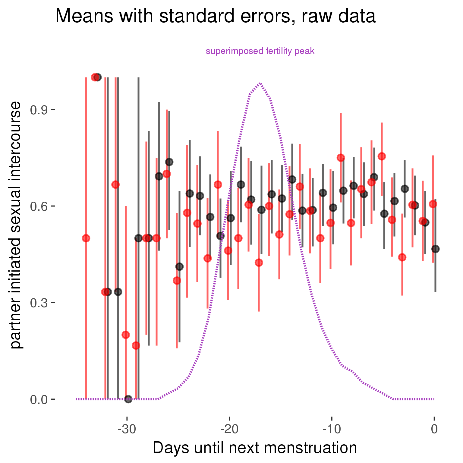
Forward-counted
model %>%
plot_curve(diary %>% filter(minimum_cycle_length_diary <= 36, minimum_cycle_length_diary > 20) %>% mutate(RCD = FCD, fertile = prc_stirn_b_forward_counted), caption_x = "Days since last menstruation")outcome = names(model@frame)[1]
outcome_label = recode(str_replace_all(str_replace_all(str_replace_all(outcome, "_", " "), " pair", "-pair"), " 1", ""),
"desirability 1" = "self-perceived desirability",
"NARQ admiration" = "narcissistic admiration",
"NARQ rivalry" = "narcissistic rivalry",
"extra-pair" = "extra-pair desire & behaviour",
"had sexual intercourse" = "sexual intercourse")
library(ggplot2)
# form a subset and run the model without the hormonal contraception and the fertility predictors
tmp = diary %>%
filter(!is.na(fertile), !is.na(included),
RCD > -1 * minimum_cycle_length_diary, RCD > -40)
new_form = update.formula(formula(model), new = . ~ . - fertile * included)
tmp$residuals = residuals(update(model, new_form, data = tmp , na.action = na.exclude))
tmp = tmp %>%
filter(!is.na(RCD), !is.na(residuals))
rcd_min = min(tmp$RCD)
tmp$real = FALSE
tmp_before = tmp
tmp_before$RCD = tmp_before$RCD + min(tmp$RCD) - 1
tmp_after = tmp
tmp_after$RCD = tmp_after$RCD - min(tmp$RCD) + 1
tmp$real = TRUE
tmp = bind_rows(tmp_before %>% filter(RCD > rcd_min - 11), tmp, tmp_after %>% filter(RCD < 11))GAM smooth on residuals
Here, we partialled out menstruation and individual random effects, then superimposed estimated probability of being in the fertile window scaled to the range of the estimated means. To address the periodicity of the cycle, we prepended and appended ten days of the timeseries to the end and the beginning of the timeseries. We then estimated the GAM and cut off the appended subsets before plotting.
tryCatch({
trend_plot = ggplot(tmp,aes(x = RCD, y = residuals, colour = included)) +
stat_smooth(geom = 'smooth',size = 0.8, fill = "#9ECAE1", method = 'gam', formula = y ~ s(x))
}, error = function(e){cat_message(e, "danger")})
tryCatch({
trend_data = ggplot_build(trend_plot)$data[[1]]
}, error = function(e){cat_message(e, "danger")})
trend_data$RCD = round(trend_data$x)
trend_data = left_join(trend_data, tmp %>% select(real, RCD,fertile) %>% unique(), by = "RCD")
trend_data %>%
filter(real == TRUE) %>%
mutate(superimposed = ( ( (fertile - 0.01)/0.58) * (max(y)-min(y) ) ) + min(y) ) ->
trend_data
ggplot(trend_data) +
geom_ribbon(aes(x = x, ymin = ymin, ymax = ymax, fill = factor(group)), alpha = 0.2) +
geom_line(aes(x = x, y = y, colour = factor(group)), size = 0.8, stat = "identity") +
scale_x_continuous(caption_x) +
geom_line(aes(x = x, y = superimposed), color = "#a83fbf", size = 1, linetype = 'dashed') +
annotate("text",x = mean(trend_data$x), y = max(trend_data$superimposed,na.rm=T) + 0.1, label = 'superimposed fertility peak', color = "#a83fbf") +
scale_y_continuous(outcome_label) +
ggtitle("GAM smooth, residuals") +
scale_color_manual("Contraception status",values = c("2"="black","1"= "red"), labels = c("2"="hormonally\ncontracepting","1"="cycling"), guide = F) +
scale_fill_manual("Contraception status",values = c("2"="black","1"= "red"), labels = c("2"="hormonally\ncontracepting","1"="cycling"), guide = F)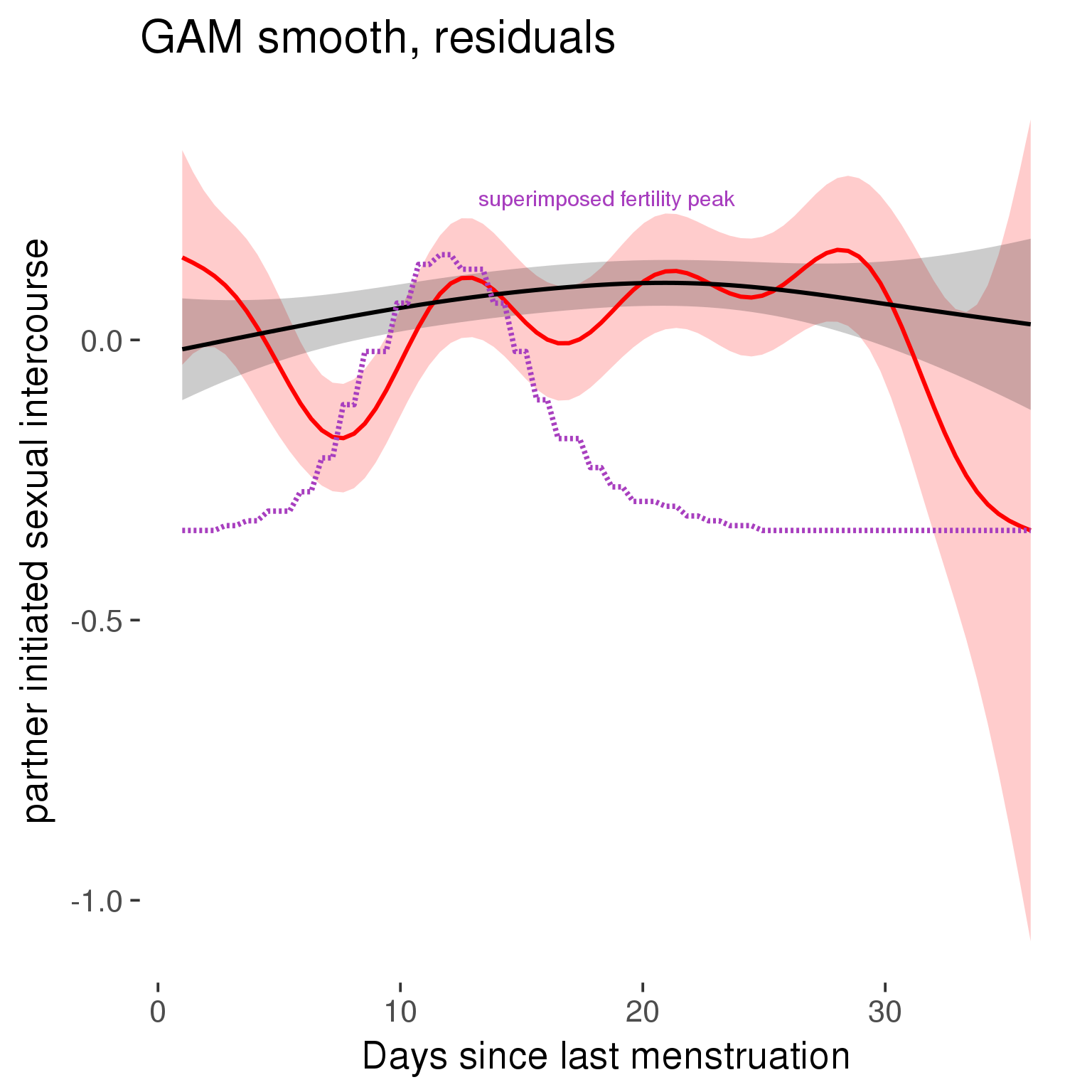
GAM smooth on raw data
As before, but without partialling anything out.
tryCatch({
trend_plot = ggplot(tmp,aes_string(x = "RCD", y = outcome, colour = "included")) +
stat_smooth(geom = 'smooth',size = 0.8, fill = "#9ECAE1", method = 'gam', formula = y ~ s(x))
}, error = function(e){cat_message(e, "danger")})
tryCatch({
trend_data = ggplot_build(trend_plot)$data[[1]]
}, error = function(e){cat_message(e, "danger")})
trend_data$RCD = round(trend_data$x)
trend_data = left_join(trend_data, tmp %>% select(real, RCD,fertile) %>% unique(), by = "RCD")
trend_data %>%
filter(real == TRUE) %>%
mutate(superimposed = ( ( (fertile - 0.01)/0.58) * (max(y)-min(y) ) ) + min(y) ) ->
trend_data
plot1b = ggplot(trend_data) +
geom_ribbon(aes(x = x, ymin = ymin, ymax = ymax, fill = factor(group)), alpha = 0.2) +
geom_line(aes(x = x, y = y, colour = factor(group)), size = 0.8, stat = "identity") +
scale_x_continuous(caption_x) +
geom_line(aes(x = x, y = superimposed), color = "#a83fbf", size = 1, linetype = 'dashed') +
annotate("text",x = mean(trend_data$x), y = max(trend_data$superimposed,na.rm=T) + 0.1, label = 'superimposed fertility peak', color = "#a83fbf") +
scale_y_continuous(outcome_label) +
ggtitle("GAM smooth, raw data") +
scale_color_manual("Contraception status",values = c("2"="black","1"= "red"), labels = c("2"="hormonally\ncontracepting","1"="cycling"), guide = F) +
scale_fill_manual("Contraception status",values = c("2"="black","1"= "red"), labels = c("2"="hormonally\ncontracepting","1"="cycling"), guide = F)
suppressWarnings(print(plot1b))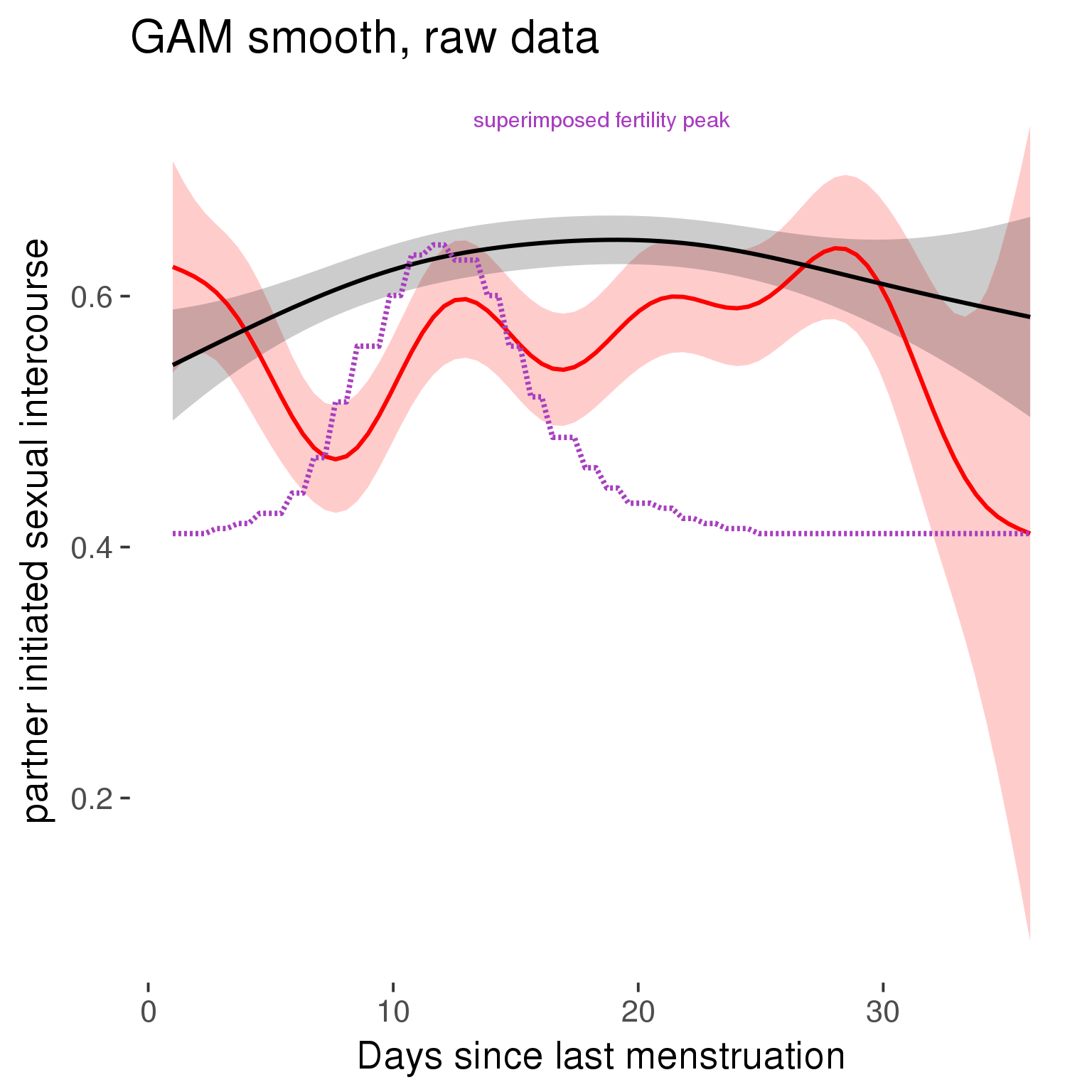
Means and standard errors over raw data
Nothing partialled out, just straight means with bootstrapped confidence intervals.
tryCatch({
trend_plot = ggplot(tmp,aes_string(x = "RCD", y = outcome, colour = "included")) +
geom_pointrange(size = 0.8, stat = 'summary', fun.data = "mean_cl_boot")
}, error = function(e){cat_message(e, "danger")})
tryCatch({
trend_data = ggplot_build(trend_plot)$data[[1]]
}, error = function(e){cat_message(e, "danger")})
trend_data$RCD = round(trend_data$x)
trend_data = left_join(trend_data, tmp %>% select(real, RCD,fertile) %>% unique(), by = "RCD")
trend_data %>%
filter(real == TRUE) %>%
mutate(superimposed = ( ( (fertile - 0.01)/0.58) * (max(y)-min(y) ) ) + min(y) ) ->
trend_data
plot3 = ggplot(trend_data) +
geom_pointrange(aes(x = x, y = y, ymin = ymin,ymax = ymax, colour = factor(group)), size = 0.8, stat = "identity", alpha = 0.6, position = position_dodge(width = .5)) +
scale_x_continuous("Days until next menstruation") +
geom_line(aes(x= x, y = superimposed), color = "#a83fbf", size = 1, linetype = 'dashed') +
annotate("text",x = mean(trend_data$x), y = max(trend_data$superimposed,na.rm=T) + 0.1, label = 'superimposed fertility peak', color = "#a83fbf") +
scale_y_continuous(outcome_label) +
ggtitle("Means with standard errors, raw data") +
scale_color_manual("Contraception status",values = c("2"="black","1"= "red"), labels = c("2"="hormonally\ncontracepting","1"="cycling"), guide = F) +
scale_fill_manual("Contraception status",values = c("2"="black","1"= "red"), labels = c("2"="hormonally\ncontracepting","1"="cycling"), guide = F)
suppressWarnings(print(plot3))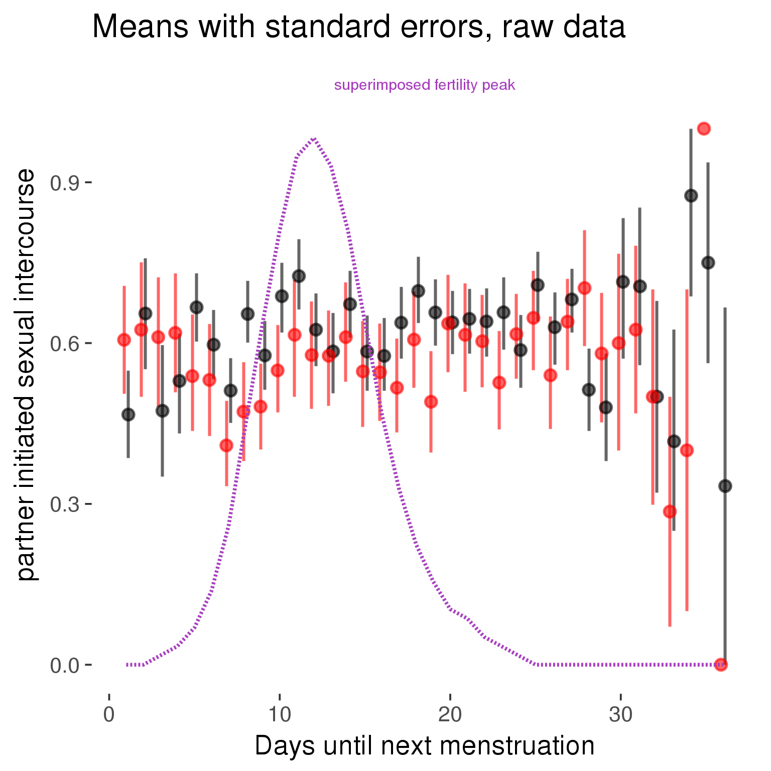
Cycle lengths from 27 to 30
Backward-counted
model %>%
plot_curve(diary %>% filter(minimum_cycle_length_diary <= 30, minimum_cycle_length_diary >= 27) %>% mutate(fertile=prc_stirn_b))outcome = names(model@frame)[1]
outcome_label = recode(str_replace_all(str_replace_all(str_replace_all(outcome, "_", " "), " pair", "-pair"), " 1", ""),
"desirability 1" = "self-perceived desirability",
"NARQ admiration" = "narcissistic admiration",
"NARQ rivalry" = "narcissistic rivalry",
"extra-pair" = "extra-pair desire & behaviour",
"had sexual intercourse" = "sexual intercourse")
library(ggplot2)
# form a subset and run the model without the hormonal contraception and the fertility predictors
tmp = diary %>%
filter(!is.na(fertile), !is.na(included),
RCD > -1 * minimum_cycle_length_diary, RCD > -40)
new_form = update.formula(formula(model), new = . ~ . - fertile * included)
tmp$residuals = residuals(update(model, new_form, data = tmp , na.action = na.exclude))
tmp = tmp %>%
filter(!is.na(RCD), !is.na(residuals))
rcd_min = min(tmp$RCD)
tmp$real = FALSE
tmp_before = tmp
tmp_before$RCD = tmp_before$RCD + min(tmp$RCD) - 1
tmp_after = tmp
tmp_after$RCD = tmp_after$RCD - min(tmp$RCD) + 1
tmp$real = TRUE
tmp = bind_rows(tmp_before %>% filter(RCD > rcd_min - 11), tmp, tmp_after %>% filter(RCD < 11))GAM smooth on residuals
Here, we partialled out menstruation and individual random effects, then superimposed estimated probability of being in the fertile window scaled to the range of the estimated means. To address the periodicity of the cycle, we prepended and appended ten days of the timeseries to the end and the beginning of the timeseries. We then estimated the GAM and cut off the appended subsets before plotting.
tryCatch({
trend_plot = ggplot(tmp,aes(x = RCD, y = residuals, colour = included)) +
stat_smooth(geom = 'smooth',size = 0.8, fill = "#9ECAE1", method = 'gam', formula = y ~ s(x))
}, error = function(e){cat_message(e, "danger")})
tryCatch({
trend_data = ggplot_build(trend_plot)$data[[1]]
}, error = function(e){cat_message(e, "danger")})
trend_data$RCD = round(trend_data$x)
trend_data = left_join(trend_data, tmp %>% select(real, RCD,fertile) %>% unique(), by = "RCD")
trend_data %>%
filter(real == TRUE) %>%
mutate(superimposed = ( ( (fertile - 0.01)/0.58) * (max(y)-min(y) ) ) + min(y) ) ->
trend_data
ggplot(trend_data) +
geom_ribbon(aes(x = x, ymin = ymin, ymax = ymax, fill = factor(group)), alpha = 0.2) +
geom_line(aes(x = x, y = y, colour = factor(group)), size = 0.8, stat = "identity") +
scale_x_continuous(caption_x) +
geom_line(aes(x = x, y = superimposed), color = "#a83fbf", size = 1, linetype = 'dashed') +
annotate("text",x = mean(trend_data$x), y = max(trend_data$superimposed,na.rm=T) + 0.1, label = 'superimposed fertility peak', color = "#a83fbf") +
scale_y_continuous(outcome_label) +
ggtitle("GAM smooth, residuals") +
scale_color_manual("Contraception status",values = c("2"="black","1"= "red"), labels = c("2"="hormonally\ncontracepting","1"="cycling"), guide = F) +
scale_fill_manual("Contraception status",values = c("2"="black","1"= "red"), labels = c("2"="hormonally\ncontracepting","1"="cycling"), guide = F)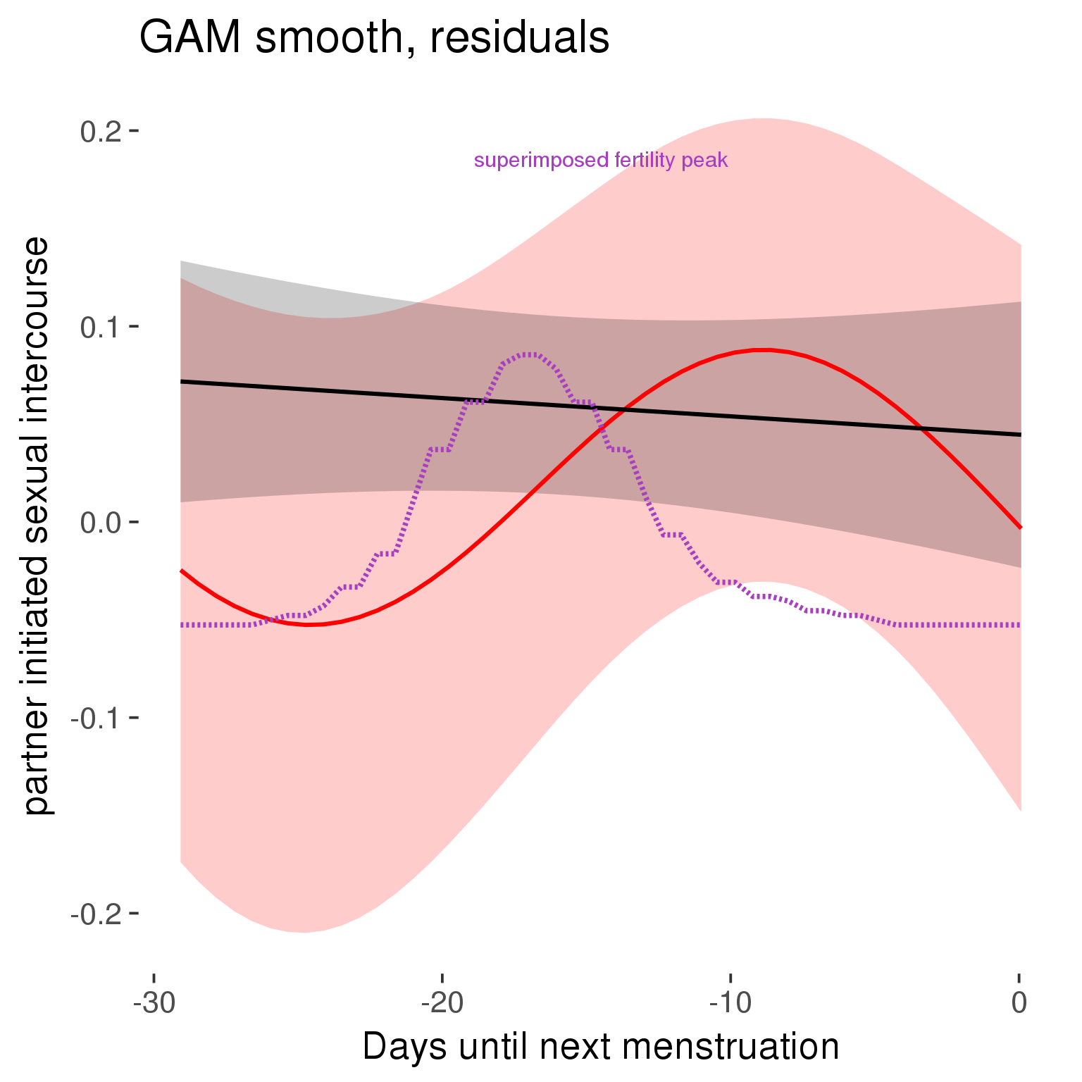
GAM smooth on raw data
As before, but without partialling anything out.
tryCatch({
trend_plot = ggplot(tmp,aes_string(x = "RCD", y = outcome, colour = "included")) +
stat_smooth(geom = 'smooth',size = 0.8, fill = "#9ECAE1", method = 'gam', formula = y ~ s(x))
}, error = function(e){cat_message(e, "danger")})
tryCatch({
trend_data = ggplot_build(trend_plot)$data[[1]]
}, error = function(e){cat_message(e, "danger")})
trend_data$RCD = round(trend_data$x)
trend_data = left_join(trend_data, tmp %>% select(real, RCD,fertile) %>% unique(), by = "RCD")
trend_data %>%
filter(real == TRUE) %>%
mutate(superimposed = ( ( (fertile - 0.01)/0.58) * (max(y)-min(y) ) ) + min(y) ) ->
trend_data
plot1b = ggplot(trend_data) +
geom_ribbon(aes(x = x, ymin = ymin, ymax = ymax, fill = factor(group)), alpha = 0.2) +
geom_line(aes(x = x, y = y, colour = factor(group)), size = 0.8, stat = "identity") +
scale_x_continuous(caption_x) +
geom_line(aes(x = x, y = superimposed), color = "#a83fbf", size = 1, linetype = 'dashed') +
annotate("text",x = mean(trend_data$x), y = max(trend_data$superimposed,na.rm=T) + 0.1, label = 'superimposed fertility peak', color = "#a83fbf") +
scale_y_continuous(outcome_label) +
ggtitle("GAM smooth, raw data") +
scale_color_manual("Contraception status",values = c("2"="black","1"= "red"), labels = c("2"="hormonally\ncontracepting","1"="cycling"), guide = F) +
scale_fill_manual("Contraception status",values = c("2"="black","1"= "red"), labels = c("2"="hormonally\ncontracepting","1"="cycling"), guide = F)
suppressWarnings(print(plot1b))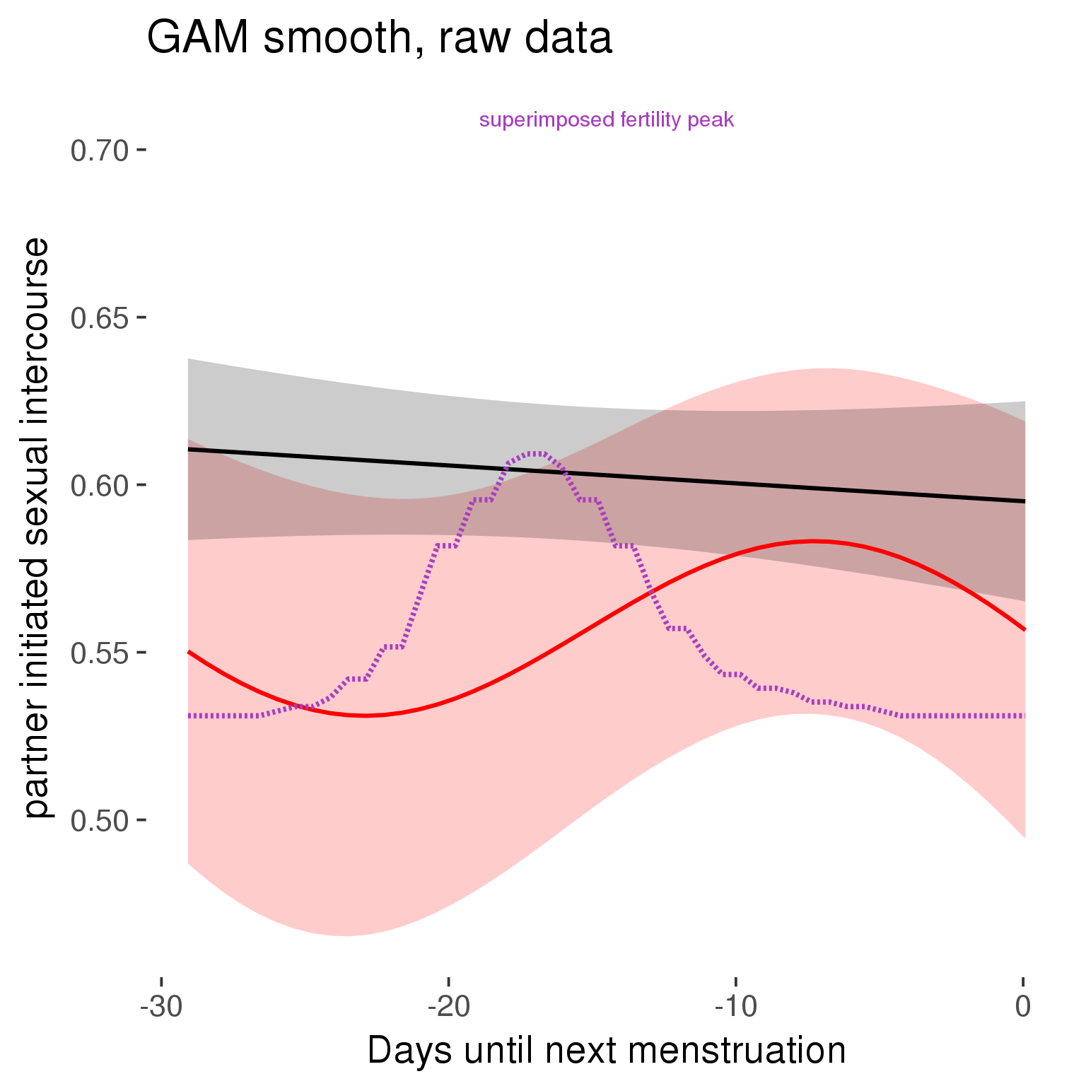
Means and standard errors over raw data
Nothing partialled out, just straight means with bootstrapped confidence intervals.
tryCatch({
trend_plot = ggplot(tmp,aes_string(x = "RCD", y = outcome, colour = "included")) +
geom_pointrange(size = 0.8, stat = 'summary', fun.data = "mean_cl_boot")
}, error = function(e){cat_message(e, "danger")})
tryCatch({
trend_data = ggplot_build(trend_plot)$data[[1]]
}, error = function(e){cat_message(e, "danger")})
trend_data$RCD = round(trend_data$x)
trend_data = left_join(trend_data, tmp %>% select(real, RCD,fertile) %>% unique(), by = "RCD")
trend_data %>%
filter(real == TRUE) %>%
mutate(superimposed = ( ( (fertile - 0.01)/0.58) * (max(y)-min(y) ) ) + min(y) ) ->
trend_data
plot3 = ggplot(trend_data) +
geom_pointrange(aes(x = x, y = y, ymin = ymin,ymax = ymax, colour = factor(group)), size = 0.8, stat = "identity", alpha = 0.6, position = position_dodge(width = .5)) +
scale_x_continuous("Days until next menstruation") +
geom_line(aes(x= x, y = superimposed), color = "#a83fbf", size = 1, linetype = 'dashed') +
annotate("text",x = mean(trend_data$x), y = max(trend_data$superimposed,na.rm=T) + 0.1, label = 'superimposed fertility peak', color = "#a83fbf") +
scale_y_continuous(outcome_label) +
ggtitle("Means with standard errors, raw data") +
scale_color_manual("Contraception status",values = c("2"="black","1"= "red"), labels = c("2"="hormonally\ncontracepting","1"="cycling"), guide = F) +
scale_fill_manual("Contraception status",values = c("2"="black","1"= "red"), labels = c("2"="hormonally\ncontracepting","1"="cycling"), guide = F)
suppressWarnings(print(plot3))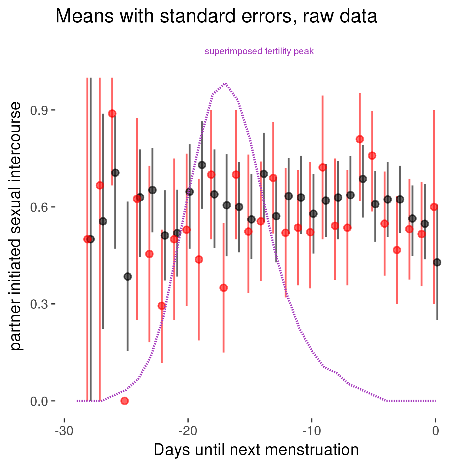
Forward-counted
model %>%
plot_curve(diary %>% filter(minimum_cycle_length_diary <= 30, minimum_cycle_length_diary >= 27) %>% mutate(RCD = FCD, fertile = prc_stirn_b_forward_counted), caption_x = "Days since last menstruation")outcome = names(model@frame)[1]
outcome_label = recode(str_replace_all(str_replace_all(str_replace_all(outcome, "_", " "), " pair", "-pair"), " 1", ""),
"desirability 1" = "self-perceived desirability",
"NARQ admiration" = "narcissistic admiration",
"NARQ rivalry" = "narcissistic rivalry",
"extra-pair" = "extra-pair desire & behaviour",
"had sexual intercourse" = "sexual intercourse")
library(ggplot2)
# form a subset and run the model without the hormonal contraception and the fertility predictors
tmp = diary %>%
filter(!is.na(fertile), !is.na(included),
RCD > -1 * minimum_cycle_length_diary, RCD > -40)
new_form = update.formula(formula(model), new = . ~ . - fertile * included)
tmp$residuals = residuals(update(model, new_form, data = tmp , na.action = na.exclude))
tmp = tmp %>%
filter(!is.na(RCD), !is.na(residuals))
rcd_min = min(tmp$RCD)
tmp$real = FALSE
tmp_before = tmp
tmp_before$RCD = tmp_before$RCD + min(tmp$RCD) - 1
tmp_after = tmp
tmp_after$RCD = tmp_after$RCD - min(tmp$RCD) + 1
tmp$real = TRUE
tmp = bind_rows(tmp_before %>% filter(RCD > rcd_min - 11), tmp, tmp_after %>% filter(RCD < 11))GAM smooth on residuals
Here, we partialled out menstruation and individual random effects, then superimposed estimated probability of being in the fertile window scaled to the range of the estimated means. To address the periodicity of the cycle, we prepended and appended ten days of the timeseries to the end and the beginning of the timeseries. We then estimated the GAM and cut off the appended subsets before plotting.
tryCatch({
trend_plot = ggplot(tmp,aes(x = RCD, y = residuals, colour = included)) +
stat_smooth(geom = 'smooth',size = 0.8, fill = "#9ECAE1", method = 'gam', formula = y ~ s(x))
}, error = function(e){cat_message(e, "danger")})
tryCatch({
trend_data = ggplot_build(trend_plot)$data[[1]]
}, error = function(e){cat_message(e, "danger")})
trend_data$RCD = round(trend_data$x)
trend_data = left_join(trend_data, tmp %>% select(real, RCD,fertile) %>% unique(), by = "RCD")
trend_data %>%
filter(real == TRUE) %>%
mutate(superimposed = ( ( (fertile - 0.01)/0.58) * (max(y)-min(y) ) ) + min(y) ) ->
trend_data
ggplot(trend_data) +
geom_ribbon(aes(x = x, ymin = ymin, ymax = ymax, fill = factor(group)), alpha = 0.2) +
geom_line(aes(x = x, y = y, colour = factor(group)), size = 0.8, stat = "identity") +
scale_x_continuous(caption_x) +
geom_line(aes(x = x, y = superimposed), color = "#a83fbf", size = 1, linetype = 'dashed') +
annotate("text",x = mean(trend_data$x), y = max(trend_data$superimposed,na.rm=T) + 0.1, label = 'superimposed fertility peak', color = "#a83fbf") +
scale_y_continuous(outcome_label) +
ggtitle("GAM smooth, residuals") +
scale_color_manual("Contraception status",values = c("2"="black","1"= "red"), labels = c("2"="hormonally\ncontracepting","1"="cycling"), guide = F) +
scale_fill_manual("Contraception status",values = c("2"="black","1"= "red"), labels = c("2"="hormonally\ncontracepting","1"="cycling"), guide = F)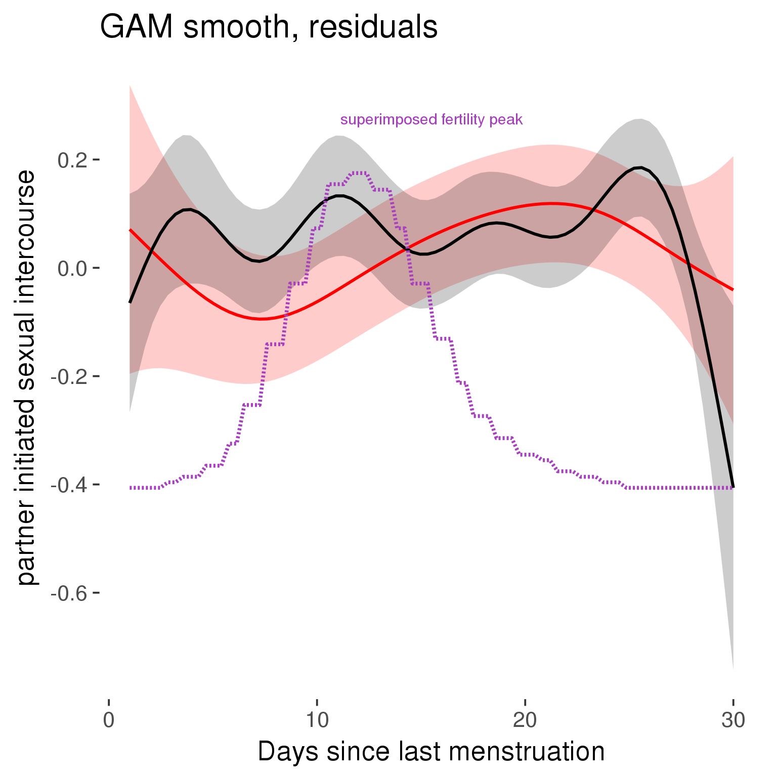
GAM smooth on raw data
As before, but without partialling anything out.
tryCatch({
trend_plot = ggplot(tmp,aes_string(x = "RCD", y = outcome, colour = "included")) +
stat_smooth(geom = 'smooth',size = 0.8, fill = "#9ECAE1", method = 'gam', formula = y ~ s(x))
}, error = function(e){cat_message(e, "danger")})
tryCatch({
trend_data = ggplot_build(trend_plot)$data[[1]]
}, error = function(e){cat_message(e, "danger")})
trend_data$RCD = round(trend_data$x)
trend_data = left_join(trend_data, tmp %>% select(real, RCD,fertile) %>% unique(), by = "RCD")
trend_data %>%
filter(real == TRUE) %>%
mutate(superimposed = ( ( (fertile - 0.01)/0.58) * (max(y)-min(y) ) ) + min(y) ) ->
trend_data
plot1b = ggplot(trend_data) +
geom_ribbon(aes(x = x, ymin = ymin, ymax = ymax, fill = factor(group)), alpha = 0.2) +
geom_line(aes(x = x, y = y, colour = factor(group)), size = 0.8, stat = "identity") +
scale_x_continuous(caption_x) +
geom_line(aes(x = x, y = superimposed), color = "#a83fbf", size = 1, linetype = 'dashed') +
annotate("text",x = mean(trend_data$x), y = max(trend_data$superimposed,na.rm=T) + 0.1, label = 'superimposed fertility peak', color = "#a83fbf") +
scale_y_continuous(outcome_label) +
ggtitle("GAM smooth, raw data") +
scale_color_manual("Contraception status",values = c("2"="black","1"= "red"), labels = c("2"="hormonally\ncontracepting","1"="cycling"), guide = F) +
scale_fill_manual("Contraception status",values = c("2"="black","1"= "red"), labels = c("2"="hormonally\ncontracepting","1"="cycling"), guide = F)
suppressWarnings(print(plot1b))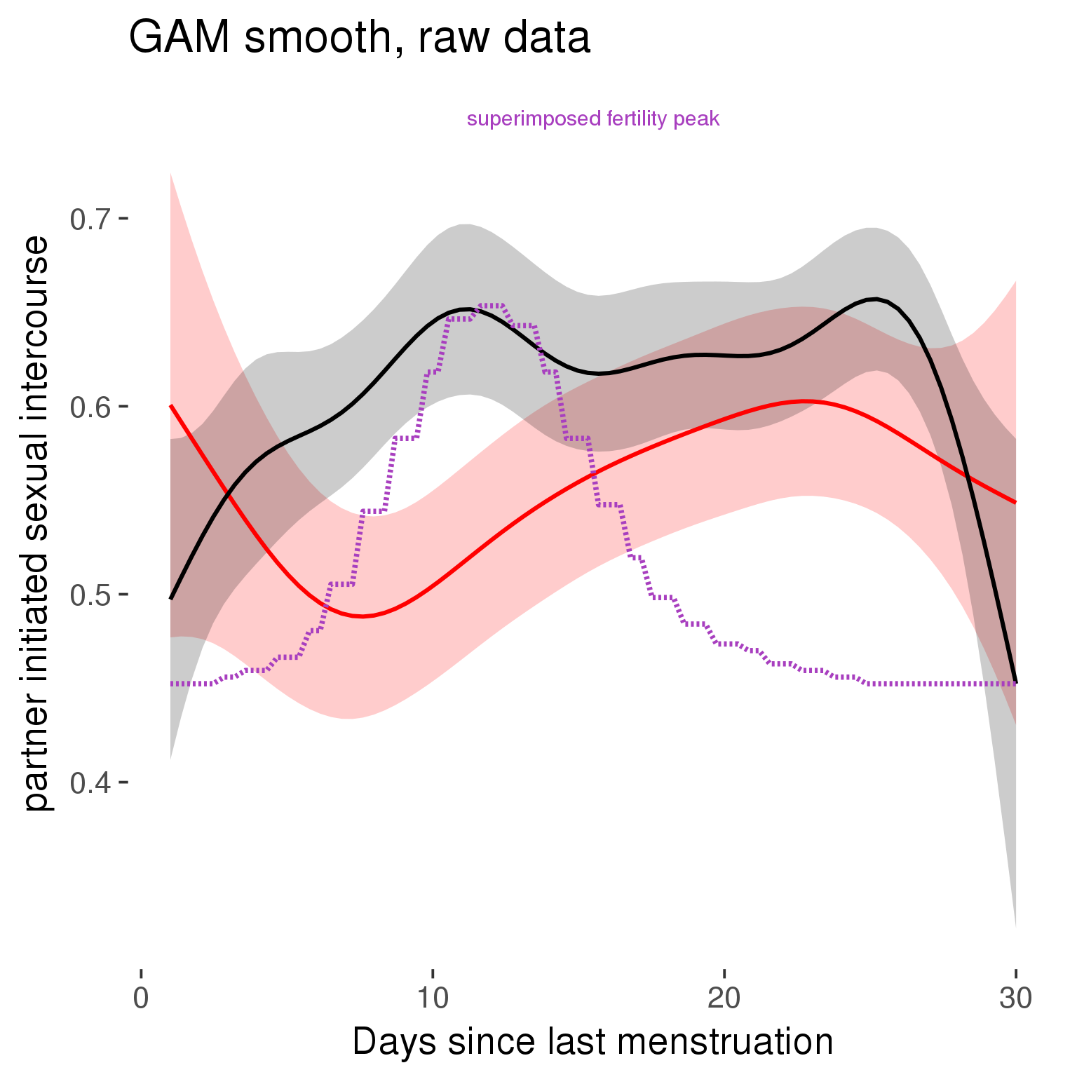
Means and standard errors over raw data
Nothing partialled out, just straight means with bootstrapped confidence intervals.
tryCatch({
trend_plot = ggplot(tmp,aes_string(x = "RCD", y = outcome, colour = "included")) +
geom_pointrange(size = 0.8, stat = 'summary', fun.data = "mean_cl_boot")
}, error = function(e){cat_message(e, "danger")})
tryCatch({
trend_data = ggplot_build(trend_plot)$data[[1]]
}, error = function(e){cat_message(e, "danger")})
trend_data$RCD = round(trend_data$x)
trend_data = left_join(trend_data, tmp %>% select(real, RCD,fertile) %>% unique(), by = "RCD")
trend_data %>%
filter(real == TRUE) %>%
mutate(superimposed = ( ( (fertile - 0.01)/0.58) * (max(y)-min(y) ) ) + min(y) ) ->
trend_data
plot3 = ggplot(trend_data) +
geom_pointrange(aes(x = x, y = y, ymin = ymin,ymax = ymax, colour = factor(group)), size = 0.8, stat = "identity", alpha = 0.6, position = position_dodge(width = .5)) +
scale_x_continuous("Days until next menstruation") +
geom_line(aes(x= x, y = superimposed), color = "#a83fbf", size = 1, linetype = 'dashed') +
annotate("text",x = mean(trend_data$x), y = max(trend_data$superimposed,na.rm=T) + 0.1, label = 'superimposed fertility peak', color = "#a83fbf") +
scale_y_continuous(outcome_label) +
ggtitle("Means with standard errors, raw data") +
scale_color_manual("Contraception status",values = c("2"="black","1"= "red"), labels = c("2"="hormonally\ncontracepting","1"="cycling"), guide = F) +
scale_fill_manual("Contraception status",values = c("2"="black","1"= "red"), labels = c("2"="hormonally\ncontracepting","1"="cycling"), guide = F)
suppressWarnings(print(plot3))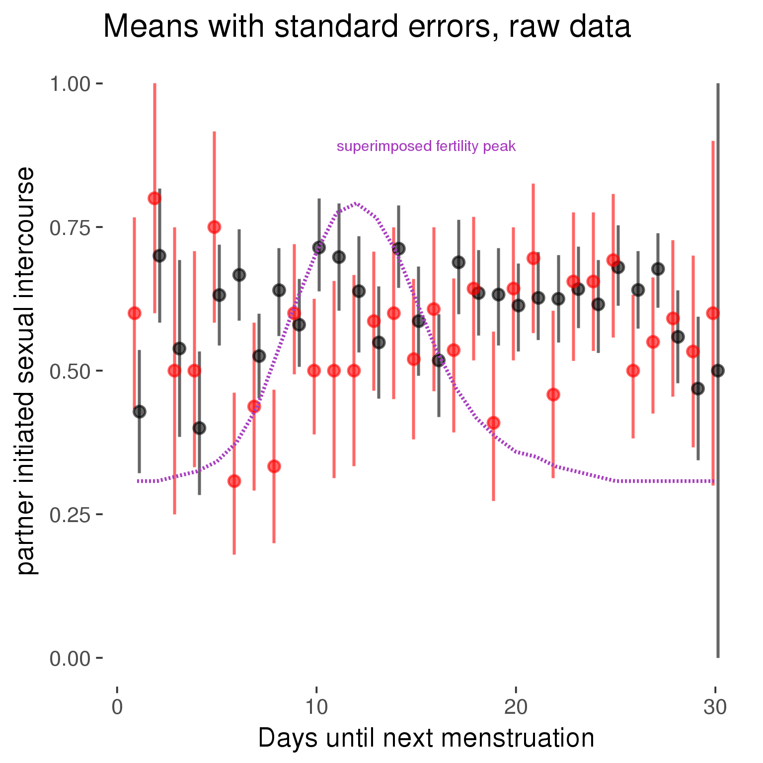
Robustness checks
M_r1: Random slopes for conception risk and menstruation
tryCatch({
# refit model with random effects for fertile and menstruation dummies
with_ind_diff = update(model, formula = . ~ . - (1| person) + (1 + fertile + menstruation | person))
# pull the random effects, format as tibble
rand = coef(with_ind_diff)$person %>%
tibble::rownames_to_column("person") %>%
mutate(person = as.numeric(person))
# pull the fixed effects
fixd = data.frame(fixef(with_ind_diff)) %>%
tibble::rownames_to_column("effect")
names(fixd) = c("effect", "pop_effect_size")
# pull apart the coefficients so that we can account for the fact that the random effect variation implicitly includes HC explaining the mean population-level effect of fertile/menstruation dummies among HC users
fixd = fixd %>%
separate(effect, c("included", "effect"), sep = ":", fill = "left") %>%
mutate(included = if_else(is.na(included), "cycling", str_replace(included, "included", "")))
fixd[2,c("included", "effect")] = c("horm_contra", "(Intercept)")
rand = rand %>%
# merge diary data on the random effects, so that we know who is a HC users and who isn't
inner_join(diary %>% select(person, included) %>% unique(), by = 'person') %>%
# gather into long format, to have the dataset by predictor
gather(effect, value, -person, -included) %>%
inner_join(fixd, by = c('effect', 'included')) %>%
# pull the fixed effects
mutate(
# only for those who are HC users, add the moderated population effect size for this effect (the random effects have the reference category mean)
value = if_else(included == "horm_contra", value + pop_effect_size, value),
effect = recode(effect, "includedhorm_contra" = "HC user",
"includedhorm_contra:fertile" = "HC user x fertile",
"includedhorm_contra:menstruationpre" = "HC user x premens.",
"includedhorm_contra:menstruationyes" = "HC user x mens.",
"menstruationyes" = "mens.",
"menstruationpre" = "premens.")) %>%
group_by(included, effect) %>%
# filter out predictors that aren't modelled as varying/random
filter(sd(value) > 0)
# plot dot plot of random effects
print(
ggplot(rand, aes(x = included, y = value, color = included, fill = included)) +
facet_wrap( ~ effect, scales = "free") +
# geom_violin(alpha = 0.4, size = 0) +
geom_dotplot(binaxis='y', dotsize = 0.1, method = "histodot") +
# geom_jitter(alpha = 0.05) +
coord_flip() +
geom_pointrange(stat = 'summary', fun.data = 'mean_sdl', color = 'darkred', size = 1.2) +
scale_color_manual("Contraception status", values = c("horm_contra"="black","cycling"= "red"), labels = c("horm_contra"="hormonally\ncontracepting","cycling"="cycling"), guide = F) +
scale_fill_manual("Contraception status", values = c("horm_contra"="black","cycling"= "red"), labels = c("horm_contra"="hormonally\ncontracepting","1"="cycling"), guide = F) +
ggtitle("M_r1: allowing participant-varying slopes", subtitle = "for the conception risk measure and the menstruation dummies") +
scale_x_discrete("Hormonal contraception", breaks = c("horm_contra", "cycling"), labels = c("yes", "no")) +
scale_y_continuous("Random effect size distribution"))
print_summary(with_ind_diff)
cat(pander(anova(model, with_ind_diff)))
}, error = function(e){
with_ind_diff = model
cat_message(e, "danger")
})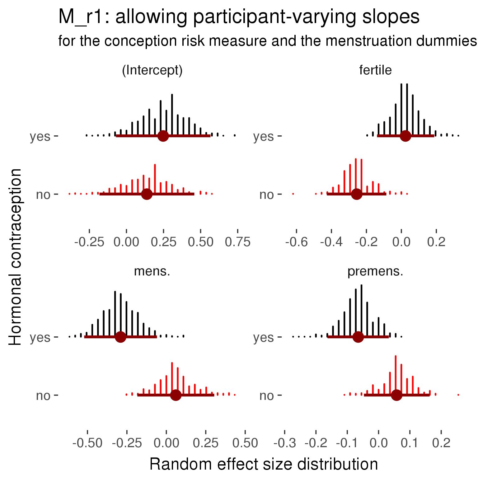
Generalized linear mixed model fit by maximum likelihood (Laplace Approximation) ['glmerMod']
Family: binomial ( probit )
Formula: partner_initiated_sexual_intercourse ~ included + menstruation +
fertile + fertile_mean + (1 + fertile + menstruation | person) +
included:menstruation + included:fertile
Data: diary
AIC BIC logLik deviance df.resid
7657 7783 -3809 7619 5729
Scaled residuals:
Min 1Q Median 3Q Max
-1.801 -1.091 0.648 0.769 1.482
Random effects:
Groups Name Variance Std.Dev. Corr
person (Intercept) 0.1060 0.326
fertile 0.1171 0.342 -0.36
menstruationpre 0.0323 0.180 0.35 -0.68
menstruationyes 0.1306 0.361 -0.54 0.82 -0.95
Number of obs: 5748, groups: person, 859
Fixed effects:
Estimate Std. Error z value Pr(>|z|)
(Intercept) 0.1389 0.0833 1.67 0.0952 .
includedhorm_contra 0.1112 0.0742 1.50 0.1341
menstruationpre 0.0580 0.0928 0.62 0.5321
menstruationyes 0.0593 0.1023 0.58 0.5619
fertile -0.2557 0.1803 -1.42 0.1562
fertile_mean 0.6279 0.3667 1.71 0.0869 .
includedhorm_contra:menstruationpre -0.1225 0.1136 -1.08 0.2808
includedhorm_contra:menstruationyes -0.3509 0.1337 -2.63 0.0086 **
includedhorm_contra:fertile 0.2787 0.2202 1.27 0.2056
---
Signif. codes: 0 '***' 0.001 '**' 0.01 '*' 0.05 '.' 0.1 ' ' 1
Correlation of Fixed Effects:
(Intr) incld_ mnstrtnp mnstrtny fertil frtl_m inclddhrm_cntr:mnstrtnp
inclddhrm_c -0.561
menstrutnpr -0.396 0.444
menstrutnys -0.341 0.385 0.246
fertile -0.432 0.599 0.444 0.325
fertile_men -0.681 -0.045 -0.011 -0.008 -0.152
inclddhrm_cntr:mnstrtnp 0.330 -0.541 -0.805 -0.199 -0.354 -0.009
inclddhrm_cntr:mnstrtny 0.258 -0.447 -0.185 -0.763 -0.245 0.004 0.230
inclddhrm_cntr:f 0.430 -0.734 -0.357 -0.264 -0.794 0.005 0.437
inclddhrm_cntr:mnstrtny
inclddhrm_c
menstrutnpr
menstrutnys
fertile
fertile_men
inclddhrm_cntr:mnstrtnp
inclddhrm_cntr:mnstrtny
inclddhrm_cntr:f 0.311
convergence code: 0
Model failed to converge with max|grad| = 0.00449993 (tol = 0.001, component 1)
| Df | AIC | BIC | logLik | deviance | Chisq | Chi Df | Pr(>Chisq) | |
|---|---|---|---|---|---|---|---|---|
| model | 10 | 7646 | 7713 | -3813 | 7626 | NA | NA | NA |
| with_ind_diff | 19 | 7657 | 7783 | -3809 | 7619 | 7.722 | 9 | 0.5624 |
robustness_check_ovu_shift(model, diary)M_e: Exclusion criteria
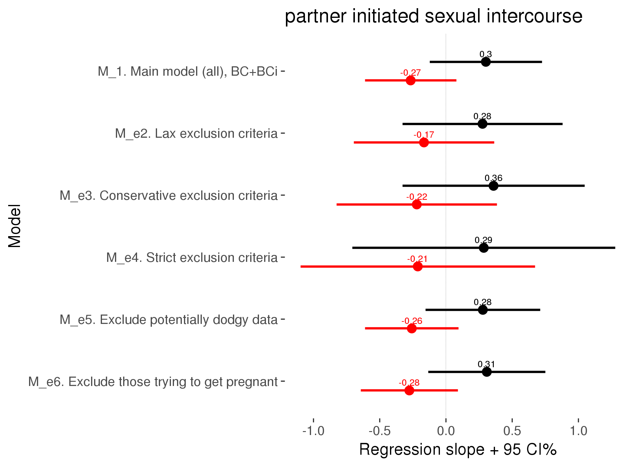
M_p: Predictors
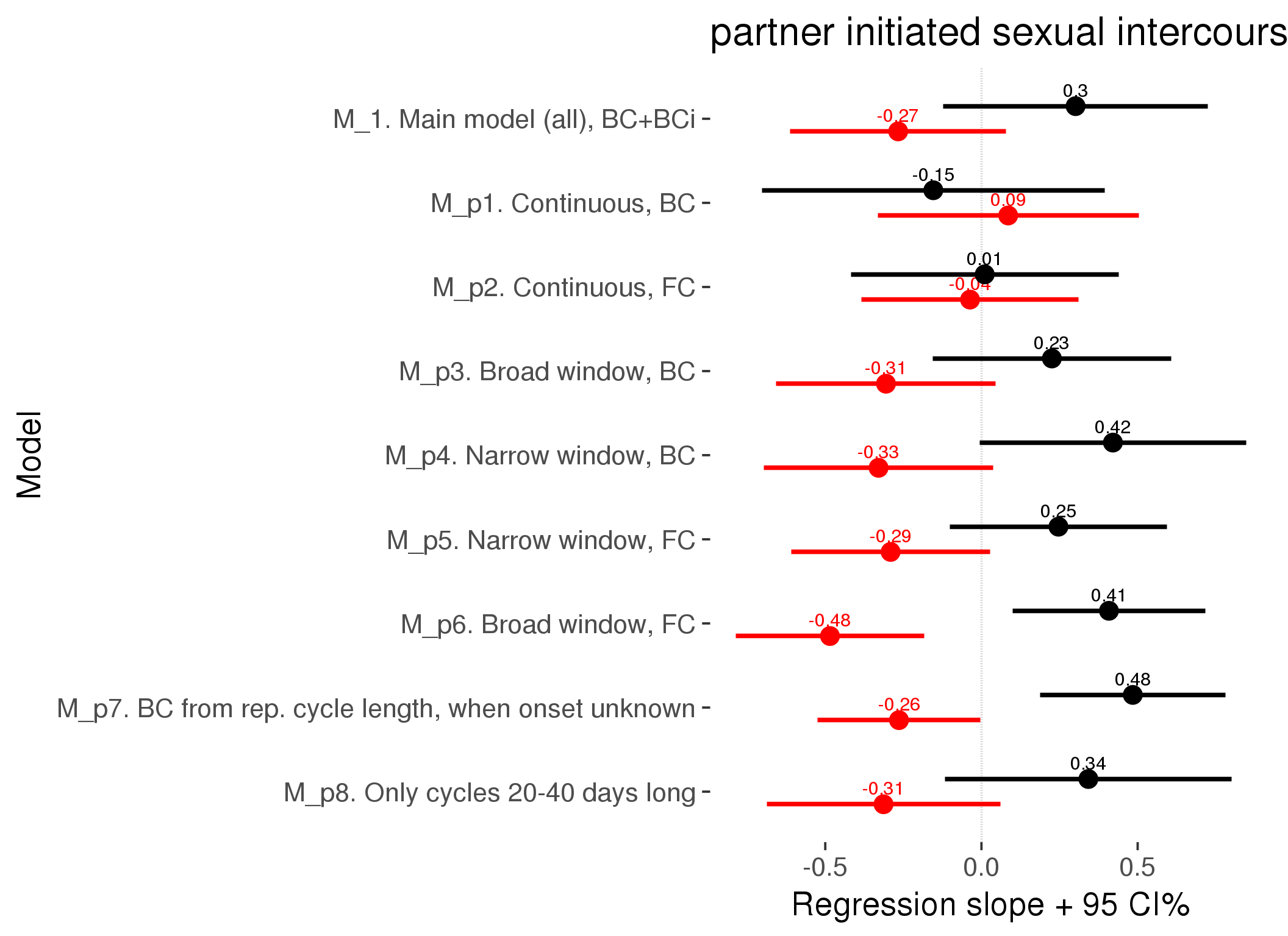
M_c: Covariates, controls, autocorrelation
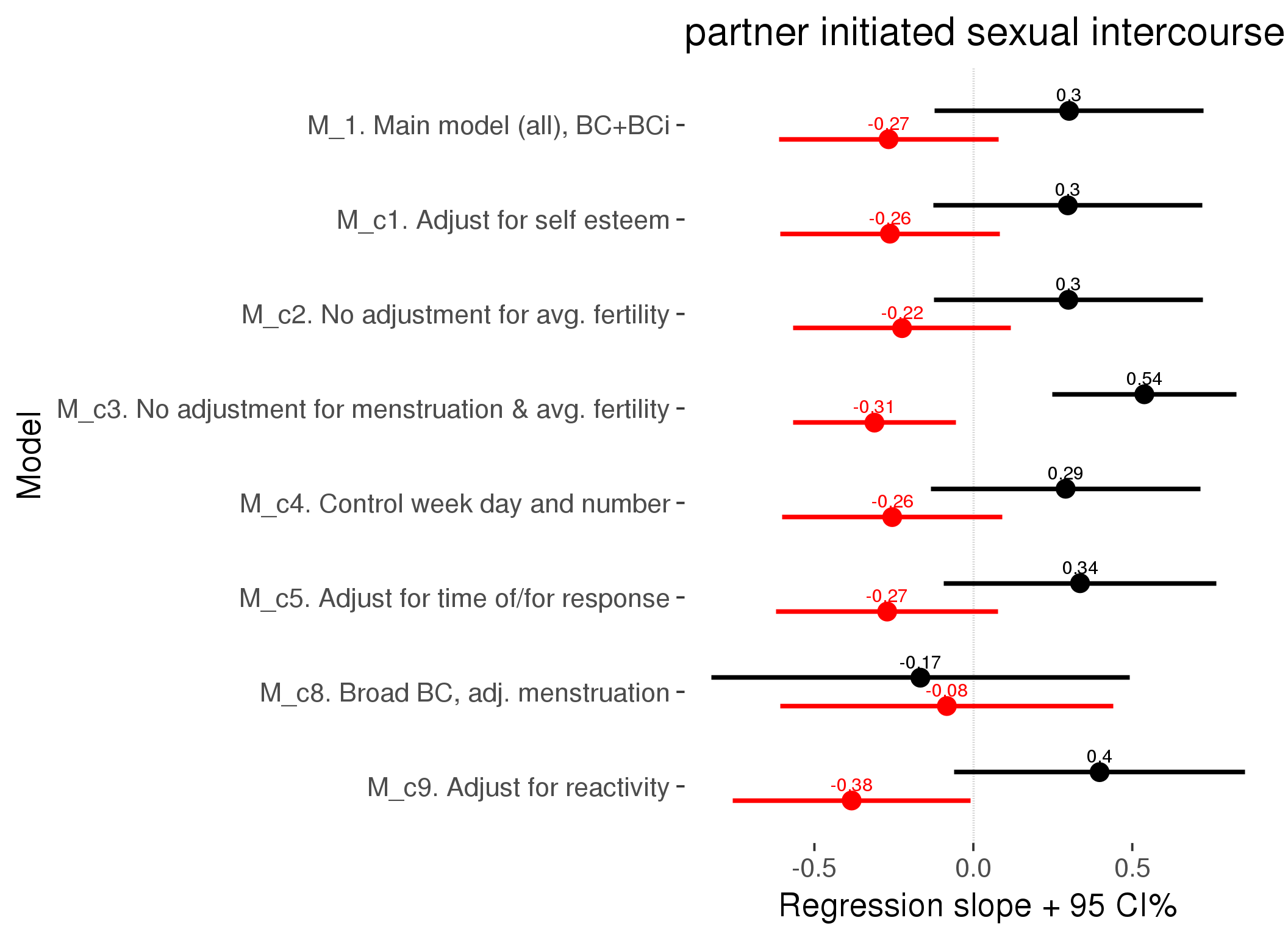
Generalized linear mixed model fit by maximum likelihood (Laplace Approximation) ['glmerMod']
Family: binomial ( probit )
AIC BIC logLik deviance df.resid
6792 6910 -3378 6756 5067
Scaled residuals:
Min 1Q Median 3Q Max
-1.676 -1.108 0.662 0.787 1.302
Random effects:
Groups Name Variance Std.Dev.
person (Intercept) 0.08828267636 0.2971240
Xr.2 s(days_filled_out):includedhorm_contra 0.00000015125 0.0003889
Xr.1 s(days_filled_out):includedcycling 0.00000001024 0.0001012
Xr.0 s(day_number):includedhorm_contra 0.00000048331 0.0006952
Xr s(day_number):includedcycling 0.00000000161 0.0000402
Number of obs: 5085, groups: person, 843; Xr.2, 8; Xr.1, 8; Xr.0, 8; Xr, 8
Fixed effects:
Estimate Std. Error z value Pr(>|z|)
X(Intercept) 0.13857 0.08690 1.59 0.111
Xincludedhorm_contra 0.06951 0.07859 0.88 0.376
Xmenstruationpre -0.00424 0.09252 -0.05 0.963
Xmenstruationyes -0.00242 0.10481 -0.02 0.982
Xfertile -0.38291 0.19081 -2.01 0.045 *
Xfertile_mean 0.82529 0.37890 2.18 0.029 *
Xincludedhorm_contra:menstruationpre -0.04745 0.11452 -0.41 0.679
Xincludedhorm_contra:menstruationyes -0.29532 0.13769 -2.15 0.032 *
Xincludedhorm_contra:fertile 0.39714 0.23358 1.70 0.089 .
Xs(day_number):includedcyclingFx1 -0.02144 0.10161 -0.21 0.833
Xs(day_number):includedhorm_contraFx1 0.06270 0.07954 0.79 0.431
Xs(days_filled_out):includedcyclingFx1 -0.00217 0.10268 -0.02 0.983
Xs(days_filled_out):includedhorm_contraFx1 -0.02128 0.08008 -0.27 0.790
---
Signif. codes: 0 '***' 0.001 '**' 0.01 '*' 0.05 '.' 0.1 ' ' 1
Family: binomial
Link function: probit
Formula:
partner_initiated_sexual_intercourse ~ included + menstruation +
fertile + fertile_mean + s(day_number, by = included) + s(days_filled_out,
by = included) + included:menstruation + included:fertile
Parametric coefficients:
Estimate Std. Error z value Pr(>|z|)
(Intercept) 0.13857 0.08526 1.63 0.104
includedhorm_contra 0.06951 0.07723 0.90 0.368
menstruationpre -0.00424 0.09074 -0.05 0.963
menstruationyes -0.00242 0.10321 -0.02 0.981
fertile -0.38291 0.18717 -2.05 0.041 *
fertile_mean 0.82529 0.37208 2.22 0.027 *
includedhorm_contra:menstruationpre -0.04745 0.11239 -0.42 0.673
includedhorm_contra:menstruationyes -0.29532 0.13549 -2.18 0.029 *
includedhorm_contra:fertile 0.39714 0.22914 1.73 0.083 .
---
Signif. codes: 0 '***' 0.001 '**' 0.01 '*' 0.05 '.' 0.1 ' ' 1
Approximate significance of smooth terms:
edf Ref.df Chi.sq p-value
s(day_number):includedcycling 1 1 0.05 0.83
s(day_number):includedhorm_contra 1 1 0.65 0.42
s(days_filled_out):includedcycling 1 1 0.00 0.98
s(days_filled_out):includedhorm_contra 1 1 0.07 0.79
R-sq.(adj) = 0.00468
glmer.ML = 6344.9 Scale est. = 1 n = 5085
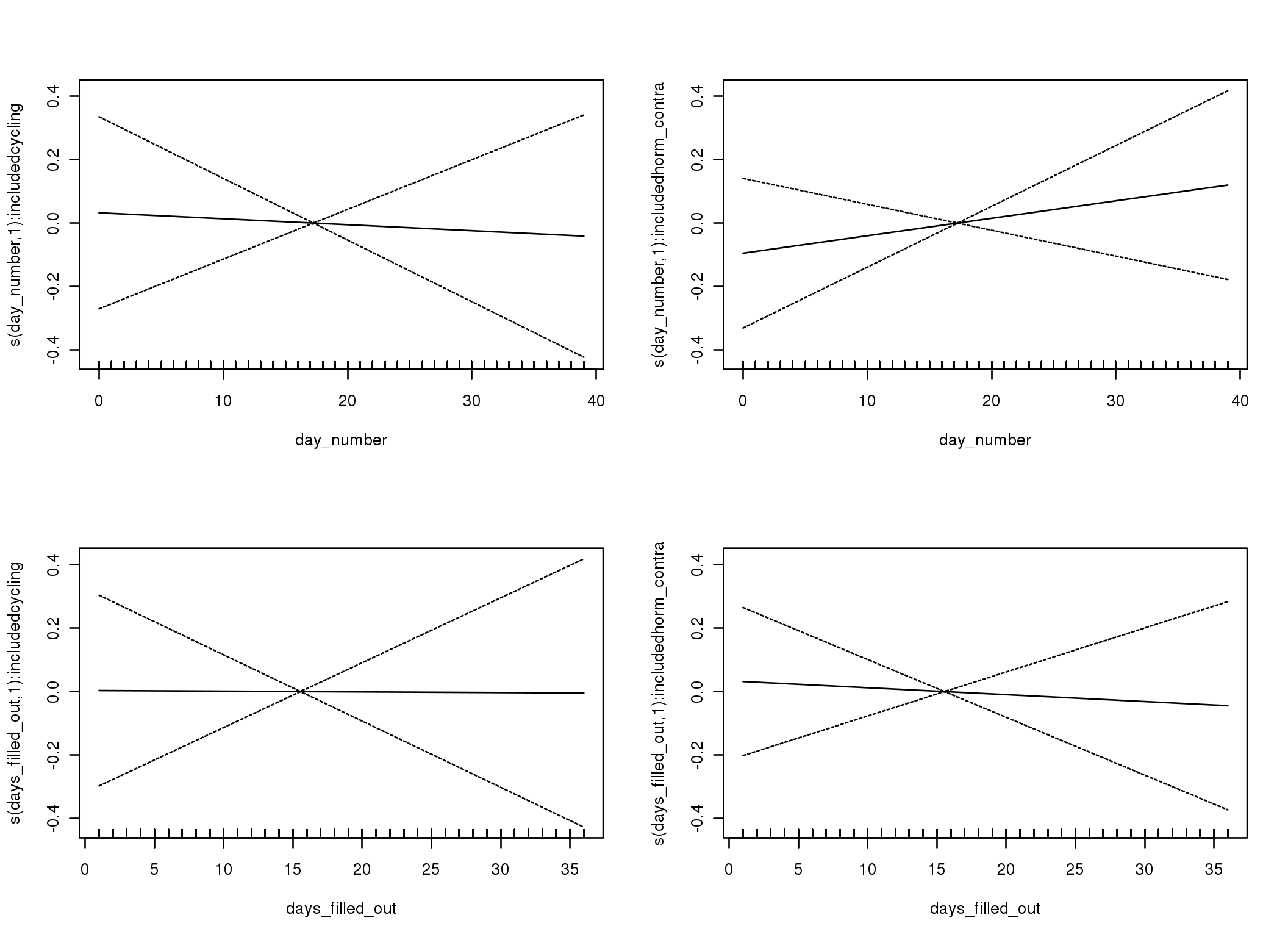
M_d: Other designs
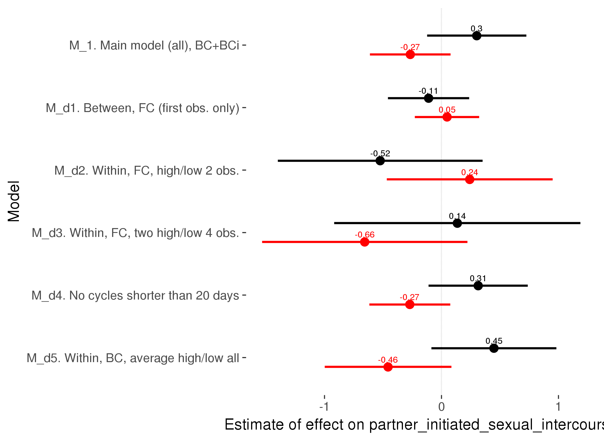
M_m1: Moderation by contraceptive method
Based on the sample with lax exclusion criteria. Users who used any hormonal contraception are classified as hormonal, users who use any awareness-based methods (counting, temperature-based) are classified as ‘fertility-awareness’, women who don’t fall into the before groups and use condoms, pessars, coitus interruptus etc. are classified as ‘barrie or abstinence’. Women who don’t use contraception or use other methods such as sterilisation are excluded from this analysis.
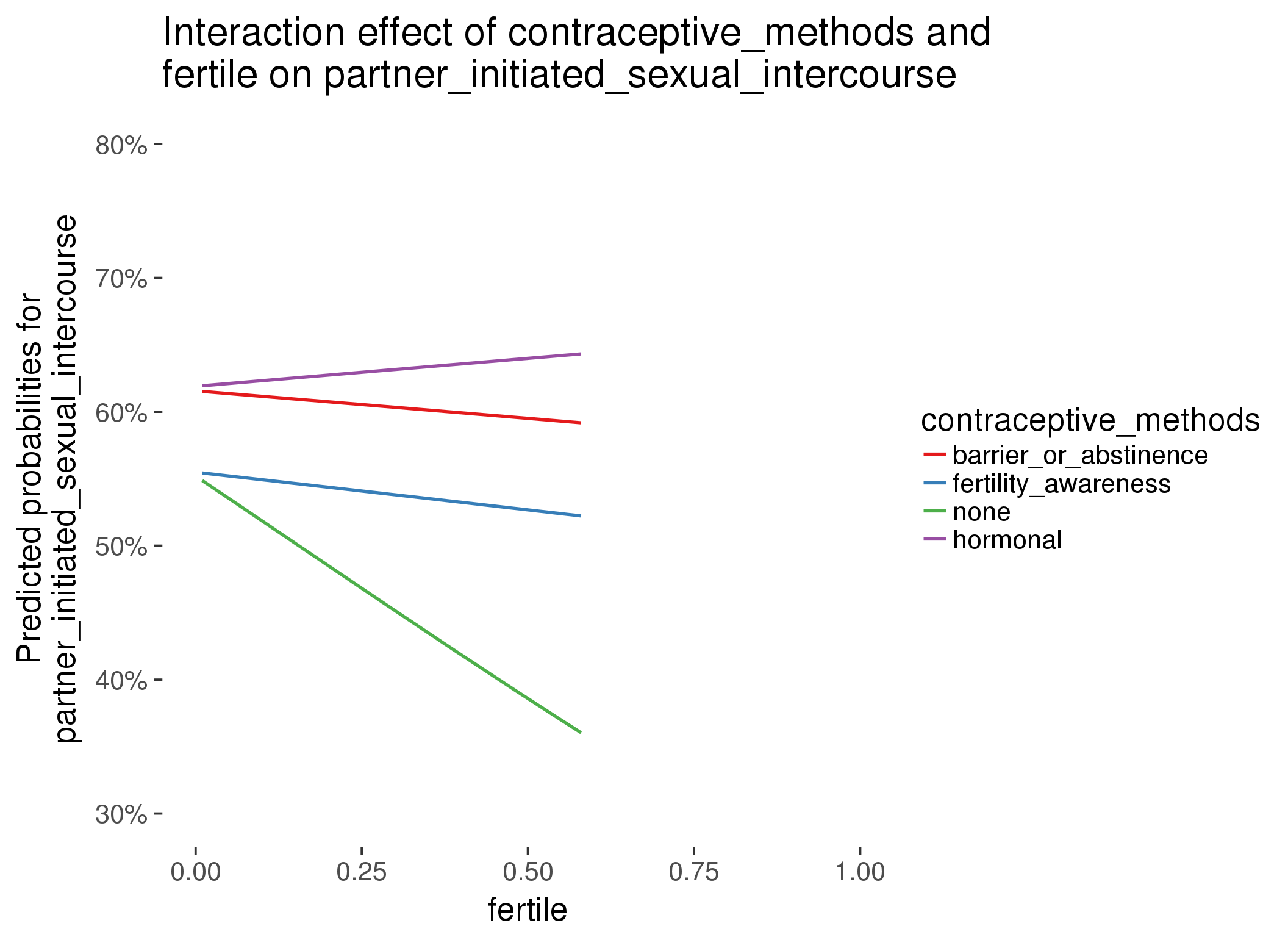
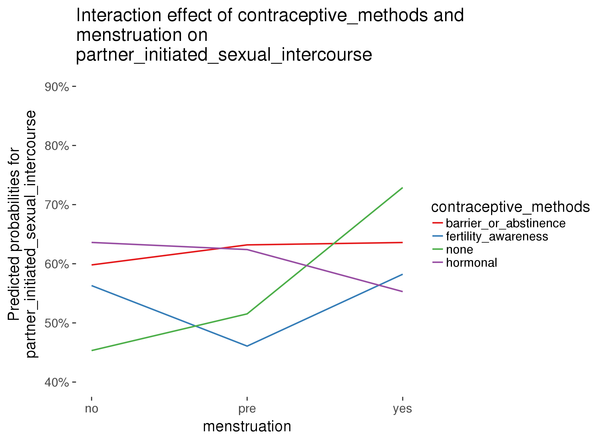
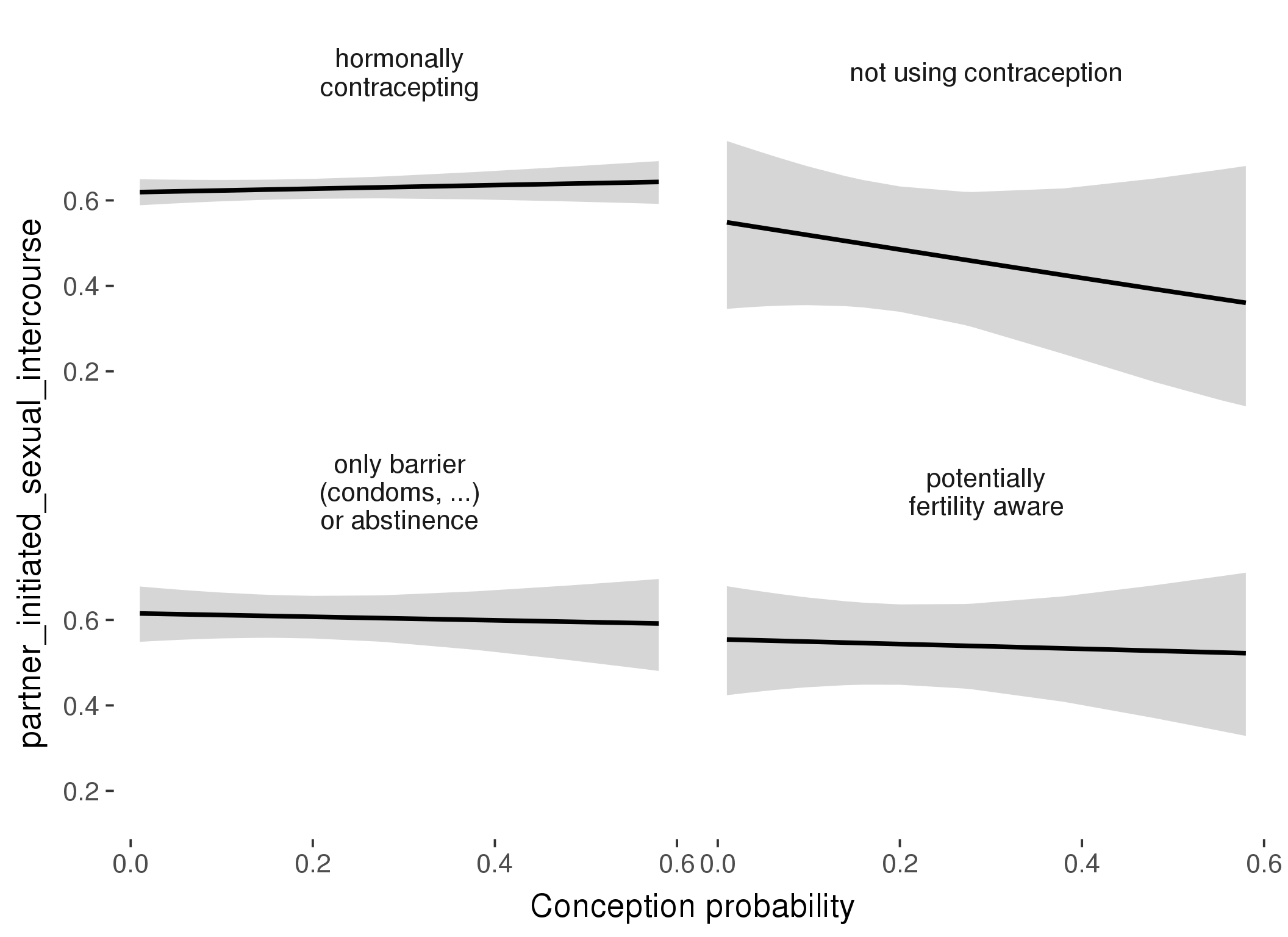
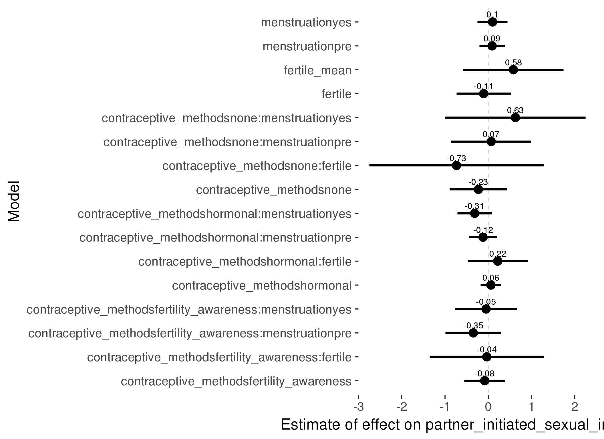
Generalized linear mixed model fit by maximum likelihood (Laplace Approximation) ['glmerMod']
Family: binomial ( probit )
Formula: partner_initiated_sexual_intercourse ~ fertile_mean + (1 | person) +
contraceptive_methods + fertile + menstruation + fertile:contraceptive_methods +
menstruation:contraceptive_methods
Data: diary
Subset: !is.na(included_lax) & contraceptive_method != "other"
AIC BIC logLik deviance df.resid
4866 4978 -2415 4830 3631
Scaled residuals:
Min 1Q Median 3Q Max
-1.752 -1.120 0.657 0.776 1.517
Random effects:
Groups Name Variance Std.Dev.
person (Intercept) 0.0961 0.31
Number of obs: 3649, groups: person, 470
Fixed effects:
Estimate Std. Error z value Pr(>|z|)
(Intercept) 0.1653 0.1387 1.19 0.23
fertile_mean 0.5809 0.5932 0.98 0.33
contraceptive_methodsfertility_awareness -0.0831 0.2408 -0.34 0.73
contraceptive_methodsnone -0.2298 0.3383 -0.68 0.50
contraceptive_methodshormonal 0.0594 0.1194 0.50 0.62
fertile -0.1068 0.3212 -0.33 0.74
menstruationpre 0.0887 0.1497 0.59 0.55
menstruationyes 0.0993 0.1771 0.56 0.58
contraceptive_methodsfertility_awareness:fertile -0.0350 0.6737 -0.05 0.96
contraceptive_methodsnone:fertile -0.7350 1.0290 -0.71 0.48
contraceptive_methodshormonal:fertile 0.2175 0.3538 0.62 0.54
contraceptive_methodsfertility_awareness:menstruationpre -0.3459 0.3304 -1.05 0.30
contraceptive_methodsnone:menstruationpre 0.0671 0.4711 0.14 0.89
contraceptive_methodshormonal:menstruationpre -0.1206 0.1670 -0.72 0.47
contraceptive_methodsfertility_awareness:menstruationyes -0.0503 0.3684 -0.14 0.89
contraceptive_methodsnone:menstruationyes 0.6275 0.8282 0.76 0.45
contraceptive_methodshormonal:menstruationyes -0.3142 0.2041 -1.54 0.12
convergence code: 0
Model failed to converge with max|grad| = 0.00844026 (tol = 0.001, component 1)
| Df | AIC | BIC | logLik | deviance | Chisq | Chi Df | Pr(>Chisq) | |
|---|---|---|---|---|---|---|---|---|
| add_main | 12 | 4858 | 4932 | -2417 | 4834 | NA | NA | NA |
| by_method | 18 | 4866 | 4978 | -2415 | 4830 | 3.134 | 6 | 0.7919 |
M_m2: Moderation by participant age
model %>%
test_moderator("age_group", diary, xlevels = 5)| Df | AIC | BIC | logLik | deviance | Chisq | Chi Df | Pr(>Chisq) | |
|---|---|---|---|---|---|---|---|---|
| with_main | 18 | 7655 | 7775 | -3810 | 7619 | NA | NA | NA |
| with_mod | 26 | 7667 | 7841 | -3808 | 7615 | 4.028 | 8 | 0.8546 |
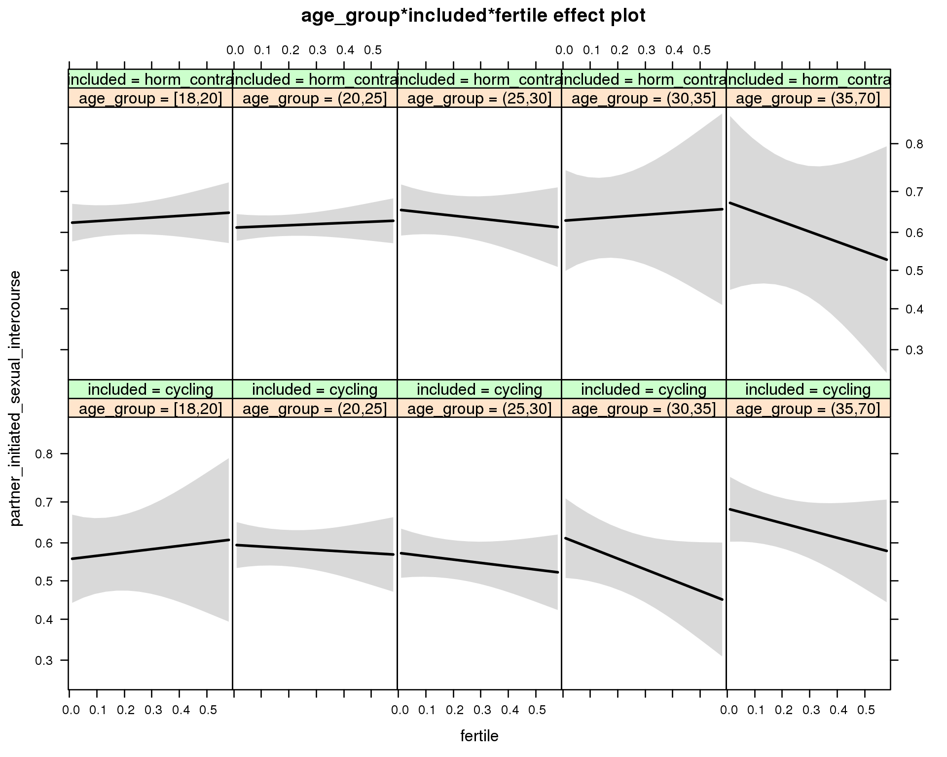
Generalized linear mixed model fit by maximum likelihood (Laplace Approximation) ['glmerMod']
Family: binomial ( probit )
Formula: partner_initiated_sexual_intercourse ~ menstruation + fertile_mean +
(1 | person) + age_group + included + fertile + menstruation:included +
age_group:included + age_group:fertile + included:fertile + age_group:included:fertile
Data: diary
AIC BIC logLik deviance df.resid
7668 7840 -3808 7616 5722
Scaled residuals:
Min 1Q Median 3Q Max
-1.903 -1.111 0.655 0.783 1.366
Random effects:
Groups Name Variance Std.Dev.
person (Intercept) 0.0874 0.296
Number of obs: 5748, groups: person, 859
Fixed effects:
Estimate Std. Error z value Pr(>|z|)
(Intercept) 0.0265 0.1635 0.16 0.8712
menstruationpre 0.0433 0.0880 0.49 0.6231
menstruationyes 0.0724 0.0961 0.75 0.4512
fertile_mean 0.5846 0.3626 1.61 0.1069
age_group(20,25] 0.0940 0.1689 0.56 0.5781
age_group(25,30] 0.0410 0.1715 0.24 0.8110
age_group(30,35] 0.1455 0.2031 0.72 0.4737
age_group(35,70] 0.3345 0.1866 1.79 0.0730 .
includedhorm_contra 0.2281 0.1711 1.33 0.1824
fertile 0.2188 0.5753 0.38 0.7037
menstruationpre:includedhorm_contra -0.1171 0.1089 -1.07 0.2824
menstruationyes:includedhorm_contra -0.3527 0.1266 -2.79 0.0053 **
age_group(20,25]:includedhorm_contra -0.1258 0.1862 -0.68 0.4994
age_group(25,30]:includedhorm_contra 0.0459 0.2031 0.23 0.8214
age_group(30,35]:includedhorm_contra -0.1316 0.2753 -0.48 0.6326
age_group(35,70]:includedhorm_contra -0.1959 0.3592 -0.55 0.5854
age_group(20,25]:fertile -0.3282 0.6248 -0.52 0.5994
age_group(25,30]:fertile -0.4403 0.6264 -0.70 0.4820
age_group(30,35]:fertile -0.9318 0.7087 -1.31 0.1886
age_group(35,70]:fertile -0.7021 0.6805 -1.03 0.3022
includedhorm_contra:fertile -0.1036 0.6169 -0.17 0.8666
age_group(20,25]:includedhorm_contra:fertile 0.2911 0.6778 0.43 0.6676
age_group(25,30]:includedhorm_contra:fertile 0.1260 0.7219 0.17 0.8615
age_group(30,35]:includedhorm_contra:fertile 0.9481 1.0133 0.94 0.3495
age_group(35,70]:includedhorm_contra:fertile -0.0727 1.1580 -0.06 0.9499
---
Signif. codes: 0 '***' 0.001 '**' 0.01 '*' 0.05 '.' 0.1 ' ' 1
convergence code: 0
Model failed to converge with max|grad| = 0.00358348 (tol = 0.001, component 1)
M_m3: Moderation by weekend
model %>%
test_moderator("weekend", diary, xlevels = 2) | Df | AIC | BIC | logLik | deviance | Chisq | Chi Df | Pr(>Chisq) | |
|---|---|---|---|---|---|---|---|---|
| with_main | 12 | 7649 | 7728 | -3812 | 7625 | NA | NA | NA |
| with_mod | 14 | 7651 | 7744 | -3811 | 7623 | 1.824 | 2 | 0.4017 |
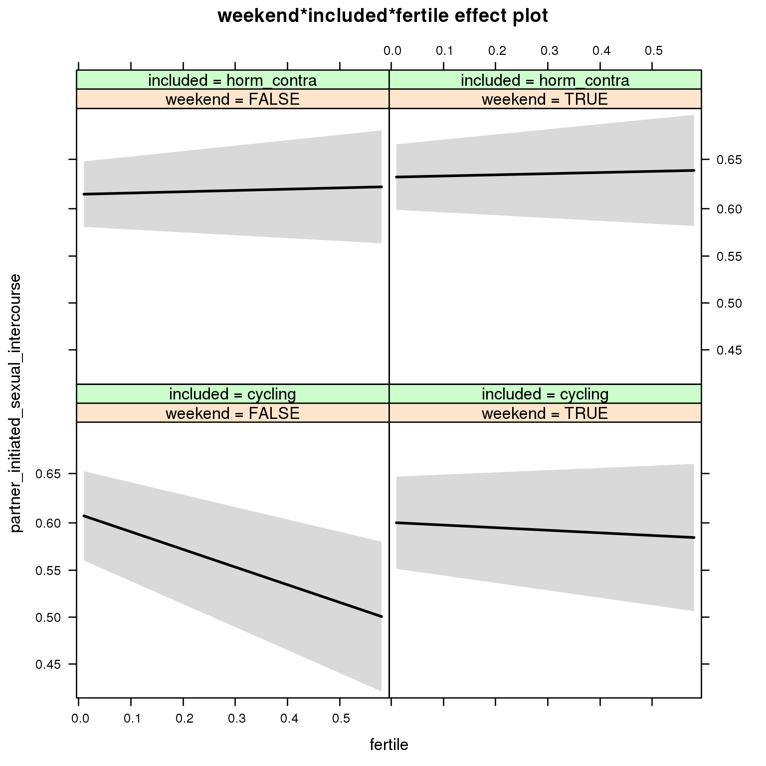
Generalized linear mixed model fit by maximum likelihood (Laplace Approximation) ['glmerMod']
Family: binomial ( probit )
Formula: partner_initiated_sexual_intercourse ~ menstruation + fertile_mean +
(1 | person) + weekend + included + fertile + menstruation:included +
weekend:included + weekend:fertile + included:fertile + weekend:included:fertile
Data: diary
AIC BIC logLik deviance df.resid
7651 7744 -3811 7623 5734
Scaled residuals:
Min 1Q Median 3Q Max
-1.774 -1.111 0.656 0.780 1.329
Random effects:
Groups Name Variance Std.Dev.
person (Intercept) 0.0913 0.302
Number of obs: 5748, groups: person, 859
Fixed effects:
Estimate Std. Error z value Pr(>|z|)
(Intercept) 0.1561 0.0906 1.72 0.0849 .
menstruationpre 0.0387 0.0880 0.44 0.6600
menstruationyes 0.0659 0.0959 0.69 0.4921
fertile_mean 0.6060 0.3623 1.67 0.0944 .
weekendTRUE -0.0224 0.0808 -0.28 0.7821
includedhorm_contra 0.0714 0.0873 0.82 0.4136
fertile -0.4735 0.2308 -2.05 0.0402 *
menstruationpre:includedhorm_contra -0.1161 0.1089 -1.07 0.2863
menstruationyes:includedhorm_contra -0.3500 0.1264 -2.77 0.0056 **
weekendTRUE:includedhorm_contra 0.0683 0.1003 0.68 0.4958
weekendTRUE:fertile 0.4038 0.2986 1.35 0.1763
includedhorm_contra:fertile 0.5079 0.2857 1.78 0.0754 .
weekendTRUE:includedhorm_contra:fertile -0.4072 0.3720 -1.09 0.2737
---
Signif. codes: 0 '***' 0.001 '**' 0.01 '*' 0.05 '.' 0.1 ' ' 1
convergence code: 0
Model failed to converge with max|grad| = 0.00305451 (tol = 0.001, component 1)
M_m4: Moderation by weekday
model %>%
test_moderator("weekday", diary, xlevels = 7)| Df | AIC | BIC | logLik | deviance | Chisq | Chi Df | Pr(>Chisq) | |
|---|---|---|---|---|---|---|---|---|
| with_main | 22 | 7654 | 7801 | -3805 | 7610 | NA | NA | NA |
| with_mod | 34 | 7662 | 7888 | -3797 | 7594 | 16.56 | 12 | 0.167 |
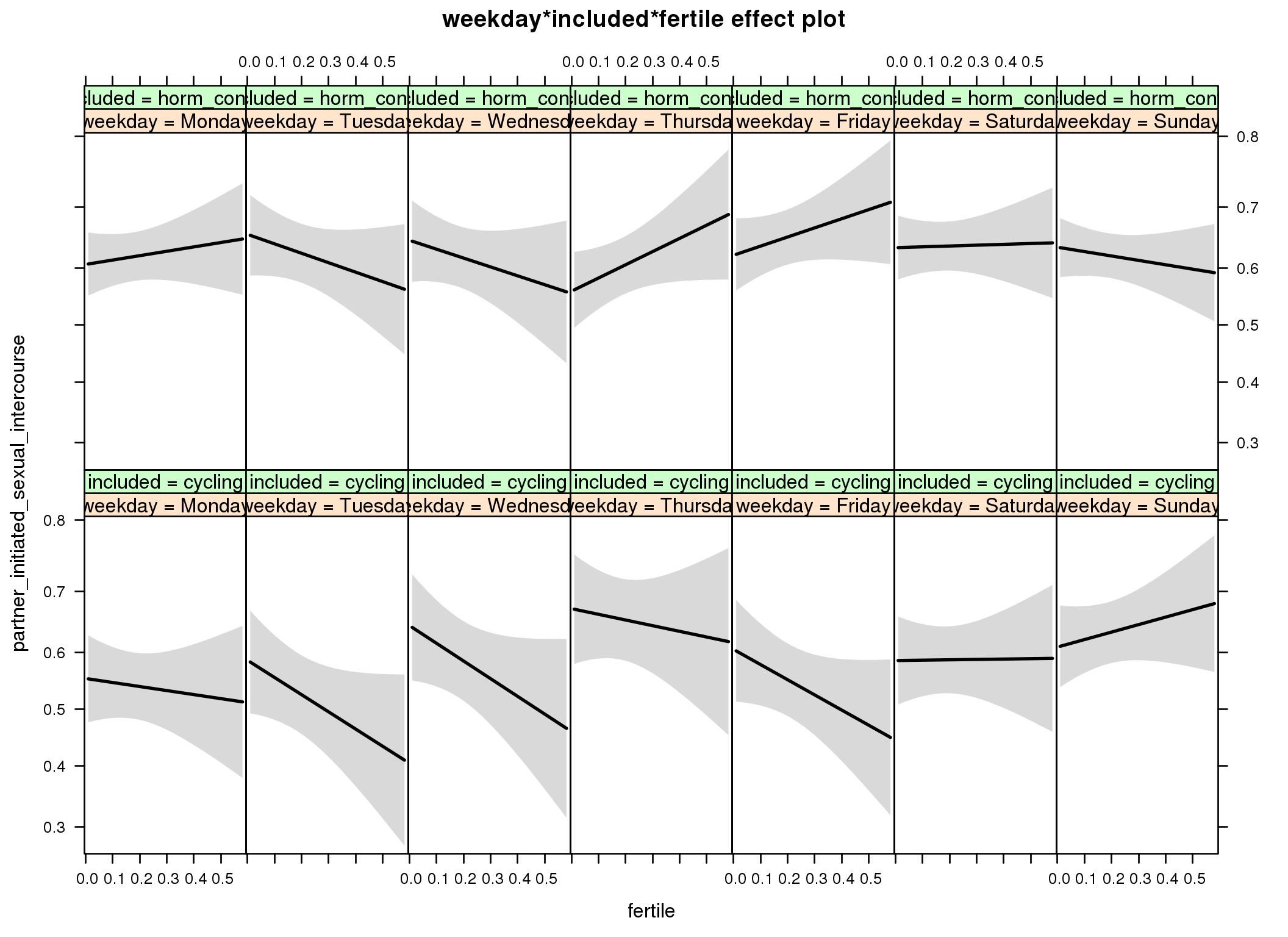
Generalized linear mixed model fit by maximum likelihood (Laplace Approximation) ['glmerMod']
Family: binomial ( probit )
Formula: partner_initiated_sexual_intercourse ~ menstruation + fertile_mean +
(1 | person) + weekday + included + fertile + menstruation:included +
weekday:included + weekday:fertile + included:fertile + weekday:included:fertile
Data: diary
AIC BIC logLik deviance df.resid
7662 7888 -3797 7594 5714
Scaled residuals:
Min 1Q Median 3Q Max
-2.003 -1.093 0.644 0.776 1.489
Random effects:
Groups Name Variance Std.Dev.
person (Intercept) 0.0915 0.303
Number of obs: 5748, groups: person, 859
Fixed effects:
Estimate Std. Error z value Pr(>|z|)
(Intercept) 0.00874 0.12023 0.07 0.9421
menstruationpre 0.04907 0.08827 0.56 0.5783
menstruationyes 0.07088 0.09625 0.74 0.4614
fertile_mean 0.63806 0.36368 1.75 0.0793 .
weekdayTuesday 0.08089 0.15143 0.53 0.5932
weekdayWednesday 0.23533 0.15525 1.52 0.1296
weekdayThursday 0.31096 0.15902 1.96 0.0505 .
weekdayFriday 0.12946 0.15063 0.86 0.3901
weekdaySaturday 0.07980 0.13872 0.57 0.5651
weekdaySunday 0.13987 0.13305 1.05 0.2931
includedhorm_contra 0.19016 0.13151 1.45 0.1482
fertile -0.17974 0.38580 -0.47 0.6413
menstruationpre:includedhorm_contra -0.12204 0.10924 -1.12 0.2639
menstruationyes:includedhorm_contra -0.35090 0.12677 -2.77 0.0056 **
weekdayTuesday:includedhorm_contra 0.05297 0.19100 0.28 0.7815
weekdayWednesday:includedhorm_contra -0.12775 0.19421 -0.66 0.5107
weekdayThursday:includedhorm_contra -0.43022 0.19469 -2.21 0.0271 *
weekdayFriday:includedhorm_contra -0.08853 0.18577 -0.48 0.6337
weekdaySaturday:includedhorm_contra -0.00502 0.17152 -0.03 0.9766
weekdaySunday:includedhorm_contra -0.06309 0.16482 -0.38 0.7019
weekdayTuesday:fertile -0.58725 0.56616 -1.04 0.2996
weekdayWednesday:fertile -0.60909 0.58609 -1.04 0.2987
weekdayThursday:fertile -0.07329 0.60657 -0.12 0.9038
weekdayFriday:fertile -0.49613 0.55146 -0.90 0.3683
weekdaySaturday:fertile 0.19629 0.52140 0.38 0.7066
weekdaySunday:fertile 0.51354 0.50332 1.02 0.3076
includedhorm_contra:fertile 0.37509 0.47562 0.79 0.4303
weekdayTuesday:includedhorm_contra:fertile -0.02941 0.71268 -0.04 0.9671
weekdayWednesday:includedhorm_contra:fertile 0.01760 0.73787 0.02 0.9810
weekdayThursday:includedhorm_contra:fertile 0.46696 0.74070 0.63 0.5284
weekdayFriday:includedhorm_contra:fertile 0.70763 0.68823 1.03 0.3039
weekdaySaturday:includedhorm_contra:fertile -0.35474 0.64720 -0.55 0.5836
weekdaySunday:includedhorm_contra:fertile -0.90457 0.62110 -1.46 0.1453
---
Signif. codes: 0 '***' 0.001 '**' 0.01 '*' 0.05 '.' 0.1 ' ' 1
convergence code: 0
Model failed to converge with max|grad| = 0.00855557 (tol = 0.001, component 1)
M_m5: Moderation by exclusion threshold
model %>%
test_moderator("included_levels", diary, xlevels = 4)| Df | AIC | BIC | logLik | deviance | Chisq | Chi Df | Pr(>Chisq) | |
|---|---|---|---|---|---|---|---|---|
| with_main | 16 | 7651 | 7757 | -3809 | 7619 | NA | NA | NA |
| with_mod | 22 | 7661 | 7808 | -3809 | 7617 | 1.263 | 6 | 0.9736 |

Generalized linear mixed model fit by maximum likelihood (Laplace Approximation) ['glmerMod']
Family: binomial ( probit )
Formula: partner_initiated_sexual_intercourse ~ menstruation + fertile_mean +
(1 | person) + included_levels + included + fertile + menstruation:included +
included_levels:included + included_levels:fertile + included:fertile +
included_levels:included:fertile
Data: diary
AIC BIC logLik deviance df.resid
7662 7808 -3809 7618 5726
Scaled residuals:
Min 1Q Median 3Q Max
-1.782 -1.105 0.652 0.785 1.274
Random effects:
Groups Name Variance Std.Dev.
person (Intercept) 0.088 0.297
Number of obs: 5748, groups: person, 859
Fixed effects:
Estimate Std. Error z value Pr(>|z|)
(Intercept) 0.1413 0.0915 1.54 0.1223
menstruationpre 0.0408 0.0880 0.46 0.6427
menstruationyes 0.0640 0.0958 0.67 0.5041
fertile_mean 0.7028 0.3679 1.91 0.0561 .
included_levelslax -0.0459 0.1483 -0.31 0.7571
included_levelsconservative 0.0253 0.1235 0.20 0.8377
included_levelsstrict -0.0791 0.1271 -0.62 0.5336
includedhorm_contra 0.1089 0.0970 1.12 0.2615
fertile -0.3402 0.2184 -1.56 0.1193
menstruationpre:includedhorm_contra -0.1175 0.1091 -1.08 0.2813
menstruationyes:includedhorm_contra -0.3462 0.1264 -2.74 0.0062 **
included_levelslax:includedhorm_contra -0.1056 0.1849 -0.57 0.5678
included_levelsconservative:includedhorm_contra -0.1071 0.1529 -0.70 0.4837
included_levelsstrict:includedhorm_contra 0.1582 0.1536 1.03 0.3030
included_levelslax:fertile 0.2197 0.5464 0.40 0.6877
included_levelsconservative:fertile 0.0434 0.4063 0.11 0.9149
included_levelsstrict:fertile 0.2572 0.4207 0.61 0.5410
includedhorm_contra:fertile 0.3171 0.3147 1.01 0.3136
included_levelslax:includedhorm_contra:fertile -0.1722 0.6550 -0.26 0.7926
included_levelsconservative:includedhorm_contra:fertile 0.1728 0.5103 0.34 0.7350
included_levelsstrict:includedhorm_contra:fertile -0.2829 0.5179 -0.55 0.5849
---
Signif. codes: 0 '***' 0.001 '**' 0.01 '*' 0.05 '.' 0.1 ' ' 1
convergence code: 0
Model failed to converge with max|grad| = 0.00431286 (tol = 0.001, component 1)
M_m6: Moderation by cycle length
model %>%
test_moderator("cycle_length_groups", diary, xlevels = 4)| Df | AIC | BIC | logLik | deviance | Chisq | Chi Df | Pr(>Chisq) | |
|---|---|---|---|---|---|---|---|---|
| with_main | 16 | 7645 | 7752 | -3807 | 7613 | NA | NA | NA |
| with_mod | 22 | 7651 | 7797 | -3804 | 7607 | 6.136 | 6 | 0.4082 |
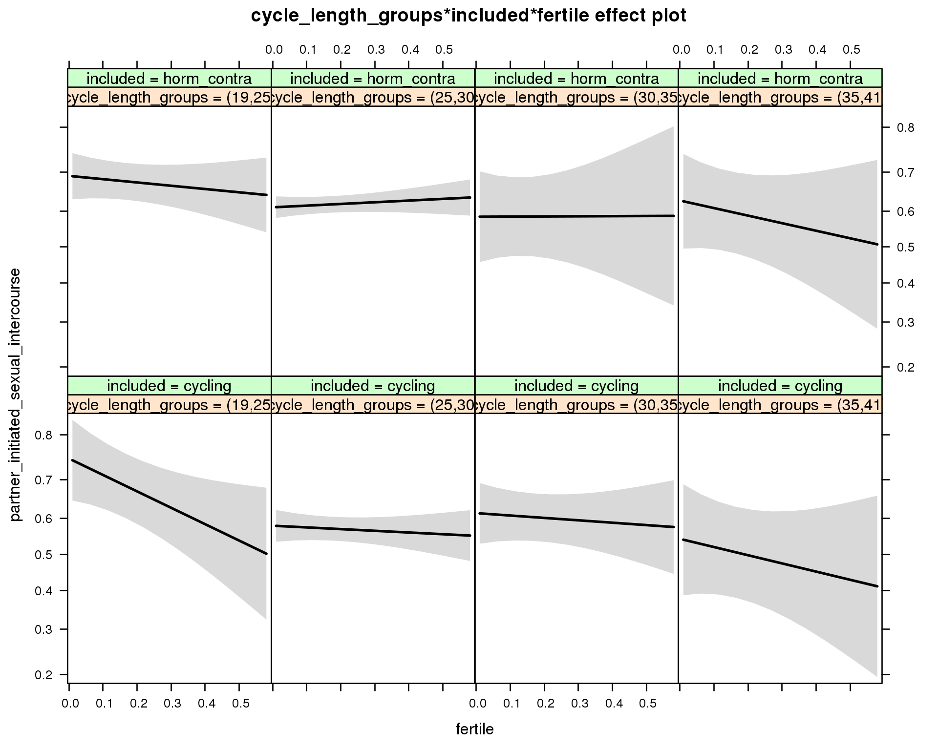
Generalized linear mixed model fit by maximum likelihood (Laplace Approximation) ['glmerMod']
Family: binomial ( probit )
Formula: partner_initiated_sexual_intercourse ~ menstruation + fertile_mean +
(1 | person) + cycle_length_groups + included + fertile +
menstruation:included + cycle_length_groups:included + cycle_length_groups:fertile +
included:fertile + cycle_length_groups:included:fertile
Data: diary
AIC BIC logLik deviance df.resid
7651 7798 -3804 7607 5726
Scaled residuals:
Min 1Q Median 3Q Max
-1.998 -1.101 0.648 0.784 1.323
Random effects:
Groups Name Variance Std.Dev.
person (Intercept) 0.0892 0.299
Number of obs: 5748, groups: person, 859
Fixed effects:
Estimate Std. Error z value Pr(>|z|)
(Intercept) 0.5694 0.1605 3.55 0.00039 ***
menstruationpre 0.0483 0.0882 0.55 0.58364
menstruationyes 0.0787 0.0965 0.82 0.41435
fertile_mean 0.4948 0.3659 1.35 0.17630
cycle_length_groups(25,30] -0.4710 0.1563 -3.01 0.00259 **
cycle_length_groups(30,35] -0.3828 0.1831 -2.09 0.03653 *
cycle_length_groups(35,41] -0.5634 0.2495 -2.26 0.02393 *
includedhorm_contra -0.1155 0.1740 -0.66 0.50670
fertile -1.1507 0.5123 -2.25 0.02471 *
menstruationpre:includedhorm_contra -0.1246 0.1091 -1.14 0.25355
menstruationyes:includedhorm_contra -0.3576 0.1269 -2.82 0.00483 **
cycle_length_groups(25,30]:includedhorm_contra 0.2505 0.1813 1.38 0.16706
cycle_length_groups(30,35]:includedhorm_contra 0.0961 0.2607 0.37 0.71248
cycle_length_groups(35,41]:includedhorm_contra 0.3904 0.3147 1.24 0.21467
cycle_length_groups(25,30]:fertile 1.0316 0.5408 1.91 0.05646 .
cycle_length_groups(30,35]:fertile 0.9828 0.6246 1.57 0.11562
cycle_length_groups(35,41]:fertile 0.5768 0.8539 0.68 0.49933
includedhorm_contra:fertile 0.9201 0.5885 1.56 0.11792
cycle_length_groups(25,30]:includedhorm_contra:fertile -0.6827 0.6241 -1.09 0.27398
cycle_length_groups(30,35]:includedhorm_contra:fertile -0.7419 0.9403 -0.79 0.43008
cycle_length_groups(35,41]:includedhorm_contra:fertile -0.8761 1.0913 -0.80 0.42209
---
Signif. codes: 0 '***' 0.001 '**' 0.01 '*' 0.05 '.' 0.1 ' ' 1
convergence code: 0
Model failed to converge with max|grad| = 0.0256235 (tol = 0.001, component 1)
M_m7: Moderation by certainty about menstruation parameters
model %>%
test_moderator("certainty_menstruation", diary)| Df | AIC | BIC | logLik | deviance | Chisq | Chi Df | Pr(>Chisq) | |
|---|---|---|---|---|---|---|---|---|
| with_main | 12 | 7650 | 7730 | -3813 | 7626 | NA | NA | NA |
| with_mod | 14 | 7654 | 7747 | -3813 | 7626 | 0.5738 | 2 | 0.7506 |
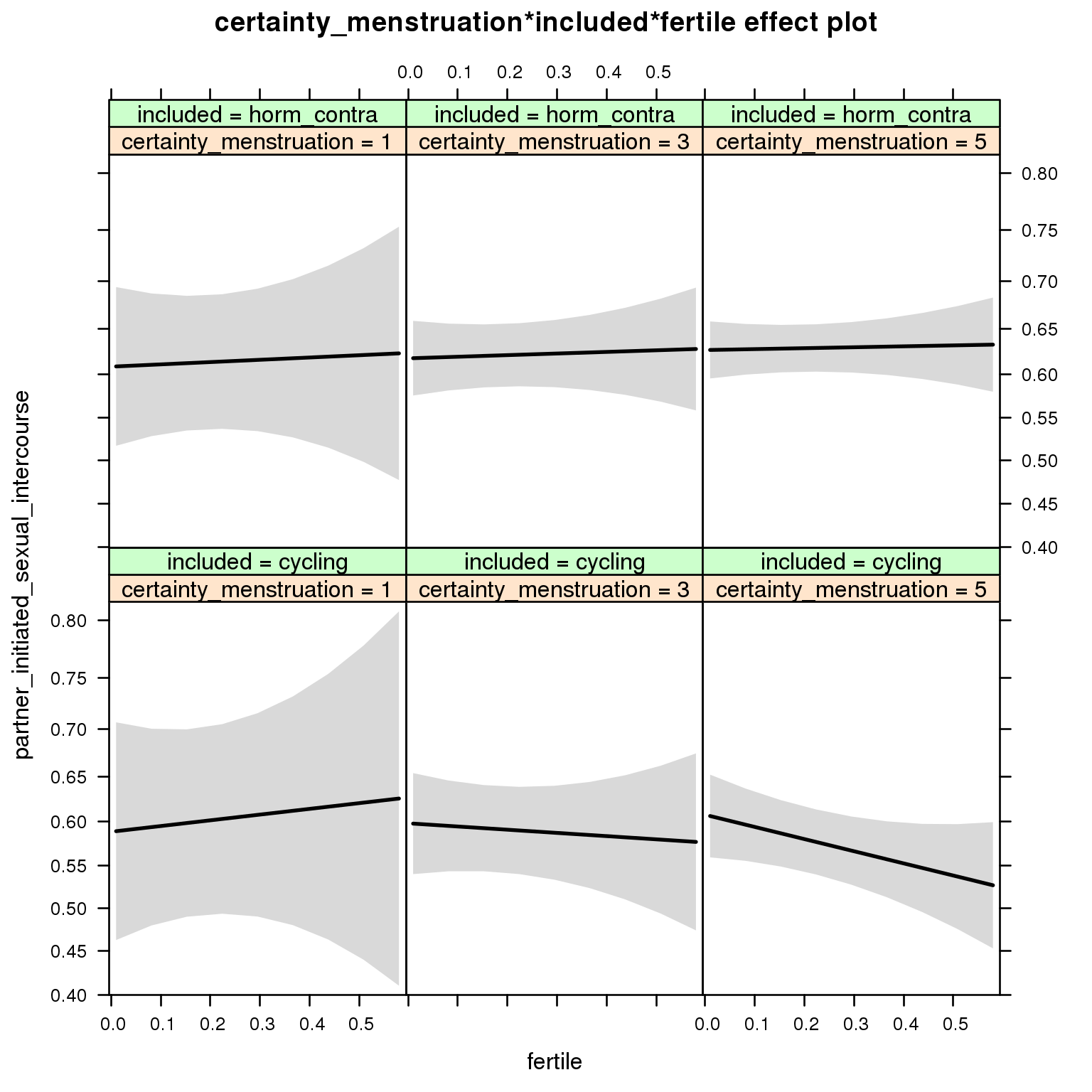
Generalized linear mixed model fit by maximum likelihood (Laplace Approximation) ['glmerMod']
Family: binomial ( probit )
Formula: partner_initiated_sexual_intercourse ~ menstruation + fertile_mean +
(1 | person) + certainty_menstruation + included + fertile +
menstruation:included + certainty_menstruation:included +
certainty_menstruation:fertile + included:fertile + certainty_menstruation:included:fertile
Data: diary
AIC BIC logLik deviance df.resid
7654 7747 -3813 7626 5734
Scaled residuals:
Min 1Q Median 3Q Max
-1.738 -1.108 0.659 0.780 1.302
Random effects:
Groups Name Variance Std.Dev.
person (Intercept) 0.0911 0.302
Number of obs: 5748, groups: person, 859
Fixed effects:
Estimate Std. Error z value Pr(>|z|)
(Intercept) 0.093026 0.218977 0.42 0.6710
menstruationpre 0.036696 0.088127 0.42 0.6771
menstruationyes 0.063422 0.095982 0.66 0.5088
fertile_mean 0.599418 0.363399 1.65 0.0990 .
certainty_menstruation 0.012396 0.049582 0.25 0.8026
includedhorm_contra 0.106165 0.265408 0.40 0.6892
fertile 0.298291 0.767330 0.39 0.6975
menstruationpre:includedhorm_contra -0.111973 0.109001 -1.03 0.3043
menstruationyes:includedhorm_contra -0.348572 0.126411 -2.76 0.0058 **
certainty_menstruation:includedhorm_contra -0.000244 0.060829 0.00 0.9968
certainty_menstruation:fertile -0.130740 0.173862 -0.75 0.4521
includedhorm_contra:fertile -0.221355 0.926883 -0.24 0.8112
certainty_menstruation:includedhorm_contra:fertile 0.120801 0.210175 0.57 0.5655
---
Signif. codes: 0 '***' 0.001 '**' 0.01 '*' 0.05 '.' 0.1 ' ' 1
convergence code: 0
Model failed to converge with max|grad| = 0.0234242 (tol = 0.001, component 1)
M_m8: Moderation by cycle regularity
model %>%
test_moderator("cycle_regularity", diary)| Df | AIC | BIC | logLik | deviance | Chisq | Chi Df | Pr(>Chisq) | |
|---|---|---|---|---|---|---|---|---|
| with_main | 14 | 7651 | 7744 | -3812 | 7623 | NA | NA | NA |
| with_mod | 18 | 7651 | 7771 | -3808 | 7615 | 7.93 | 4 | 0.09418 |
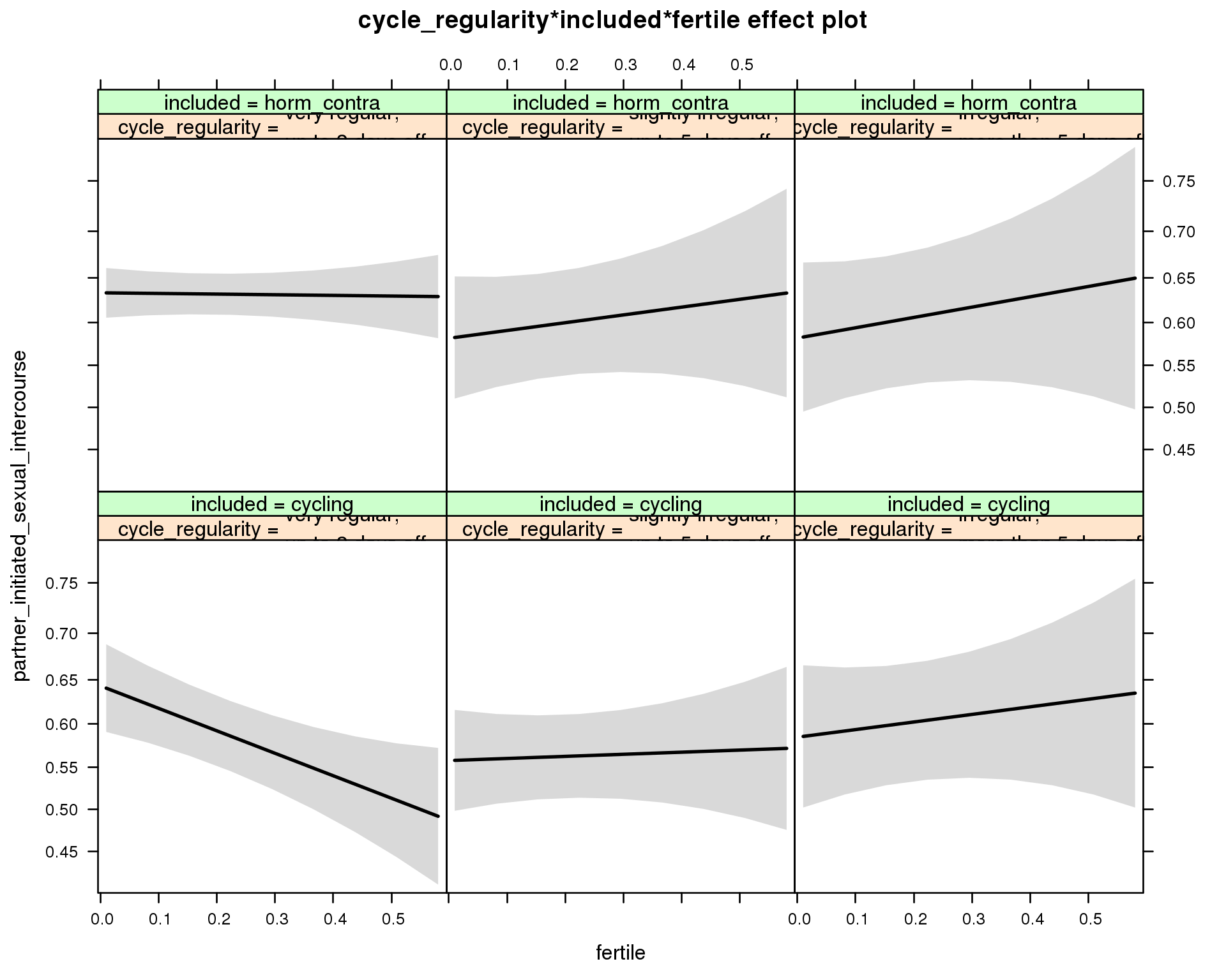
Generalized linear mixed model fit by maximum likelihood (Laplace Approximation) ['glmerMod']
Family: binomial ( probit )
Formula: partner_initiated_sexual_intercourse ~ menstruation + fertile_mean +
(1 | person) + cycle_regularity + included + fertile + menstruation:included +
cycle_regularity:included + cycle_regularity:fertile + included:fertile +
cycle_regularity:included:fertile
Data: diary
AIC BIC logLik deviance df.resid
7651 7771 -3808 7615 5730
Scaled residuals:
Min 1Q Median 3Q Max
-1.815 -1.109 0.655 0.778 1.357
Random effects:
Groups Name Variance Std.Dev.
person (Intercept) 0.0884 0.297
Number of obs: 5748, groups: person, 859
Fixed effects:
Estimate Std. Error z value
(Intercept) 0.2608 0.0966 2.70
menstruationpre 0.0261 0.0881 0.30
menstruationyes 0.0612 0.0959 0.64
fertile_mean 0.5441 0.3621 1.50
cycle_regularityslightly irregular,\nup to 5 days off -0.2225 0.0997 -2.23
cycle_regularityirregular,\nmore than 5 days off -0.1528 0.1275 -1.20
includedhorm_contra 0.0268 0.0893 0.30
fertile -0.6698 0.2346 -2.86
menstruationpre:includedhorm_contra -0.1019 0.1090 -0.93
menstruationyes:includedhorm_contra -0.3437 0.1263 -2.72
cycle_regularityslightly irregular,\nup to 5 days off:includedhorm_contra 0.0869 0.1418 0.61
cycle_regularityirregular,\nmore than 5 days off:includedhorm_contra 0.0179 0.1756 0.10
cycle_regularityslightly irregular,\nup to 5 days off:fertile 0.7322 0.3345 2.19
cycle_regularityirregular,\nmore than 5 days off:fertile 0.8961 0.4305 2.08
includedhorm_contra:fertile 0.6504 0.2717 2.39
cycle_regularityslightly irregular,\nup to 5 days off:includedhorm_contra:fertile -0.4805 0.4880 -0.98
cycle_regularityirregular,\nmore than 5 days off:includedhorm_contra:fertile -0.5690 0.6096 -0.93
Pr(>|z|)
(Intercept) 0.0070 **
menstruationpre 0.7675
menstruationyes 0.5234
fertile_mean 0.1330
cycle_regularityslightly irregular,\nup to 5 days off 0.0257 *
cycle_regularityirregular,\nmore than 5 days off 0.2305
includedhorm_contra 0.7640
fertile 0.0043 **
menstruationpre:includedhorm_contra 0.3501
menstruationyes:includedhorm_contra 0.0065 **
cycle_regularityslightly irregular,\nup to 5 days off:includedhorm_contra 0.5398
cycle_regularityirregular,\nmore than 5 days off:includedhorm_contra 0.9189
cycle_regularityslightly irregular,\nup to 5 days off:fertile 0.0286 *
cycle_regularityirregular,\nmore than 5 days off:fertile 0.0374 *
includedhorm_contra:fertile 0.0167 *
cycle_regularityslightly irregular,\nup to 5 days off:includedhorm_contra:fertile 0.3248
cycle_regularityirregular,\nmore than 5 days off:includedhorm_contra:fertile 0.3506
---
Signif. codes: 0 '***' 0.001 '**' 0.01 '*' 0.05 '.' 0.1 ' ' 1
convergence code: 0
Model failed to converge with max|grad| = 0.010458 (tol = 0.001, component 1)
M_m9: Moderation by cohabitation status
model %>%
test_moderator("cohabitation", diary)| Df | AIC | BIC | logLik | deviance | Chisq | Chi Df | Pr(>Chisq) | |
|---|---|---|---|---|---|---|---|---|
| with_main | 14 | 7649 | 7742 | -3810 | 7621 | NA | NA | NA |
| with_mod | 18 | 7652 | 7771 | -3808 | 7616 | 5.22 | 4 | 0.2654 |
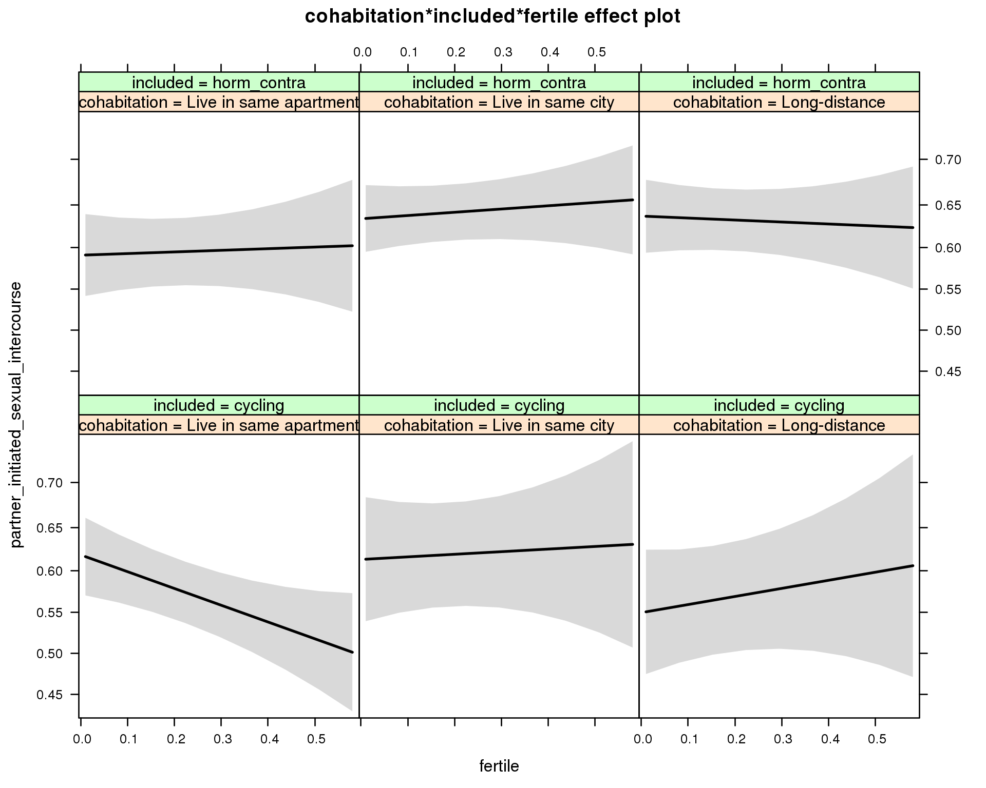
Generalized linear mixed model fit by maximum likelihood (Laplace Approximation) ['glmerMod']
Family: binomial ( probit )
Formula: partner_initiated_sexual_intercourse ~ menstruation + fertile_mean +
(1 | person) + cohabitation + included + fertile + menstruation:included +
cohabitation:included + cohabitation:fertile + included:fertile + cohabitation:included:fertile
Data: diary
AIC BIC logLik deviance df.resid
7652 7772 -3808 7616 5730
Scaled residuals:
Min 1Q Median 3Q Max
-1.805 -1.108 0.656 0.779 1.322
Random effects:
Groups Name Variance Std.Dev.
person (Intercept) 0.0893 0.299
Number of obs: 5748, groups: person, 859
Fixed effects:
Estimate Std. Error z value Pr(>|z|)
(Intercept) 0.1871 0.0927 2.02 0.0436 *
menstruationpre 0.0428 0.0879 0.49 0.6263
menstruationyes 0.0641 0.0959 0.67 0.5042
fertile_mean 0.5717 0.3632 1.57 0.1155
cohabitationLive in same city -0.0139 0.1139 -0.12 0.9028
cohabitationLong-distance -0.1772 0.1139 -1.55 0.1199
includedhorm_contra -0.0142 0.0989 -0.14 0.8858
fertile -0.5151 0.2102 -2.45 0.0143 *
menstruationpre:includedhorm_contra -0.1231 0.1089 -1.13 0.2584
menstruationyes:includedhorm_contra -0.3523 0.1264 -2.79 0.0053 **
cohabitationLive in same city:includedhorm_contra 0.1257 0.1412 0.89 0.3734
cohabitationLong-distance:includedhorm_contra 0.2973 0.1431 2.08 0.0378 *
cohabitationLive in same city:fertile 0.5949 0.3906 1.52 0.1278
cohabitationLong-distance:fertile 0.7635 0.4041 1.89 0.0589 .
includedhorm_contra:fertile 0.5650 0.3092 1.83 0.0677 .
cohabitationLive in same city:includedhorm_contra:fertile -0.5449 0.4806 -1.13 0.2569
cohabitationLong-distance:includedhorm_contra:fertile -0.8743 0.5013 -1.74 0.0812 .
---
Signif. codes: 0 '***' 0.001 '**' 0.01 '*' 0.05 '.' 0.1 ' ' 1
convergence code: 0
Model failed to converge with max|grad| = 0.00381763 (tol = 0.001, component 1)
M_m10: Moderation by relationship status
model %>%
test_moderator("relationship_status_clean", diary)| Df | AIC | BIC | logLik | deviance | Chisq | Chi Df | Pr(>Chisq) | |
|---|---|---|---|---|---|---|---|---|
| with_main | 14 | 7648 | 7741 | -3810 | 7620 | NA | NA | NA |
| with_mod | 18 | 7653 | 7773 | -3809 | 7617 | 2.363 | 4 | 0.6693 |
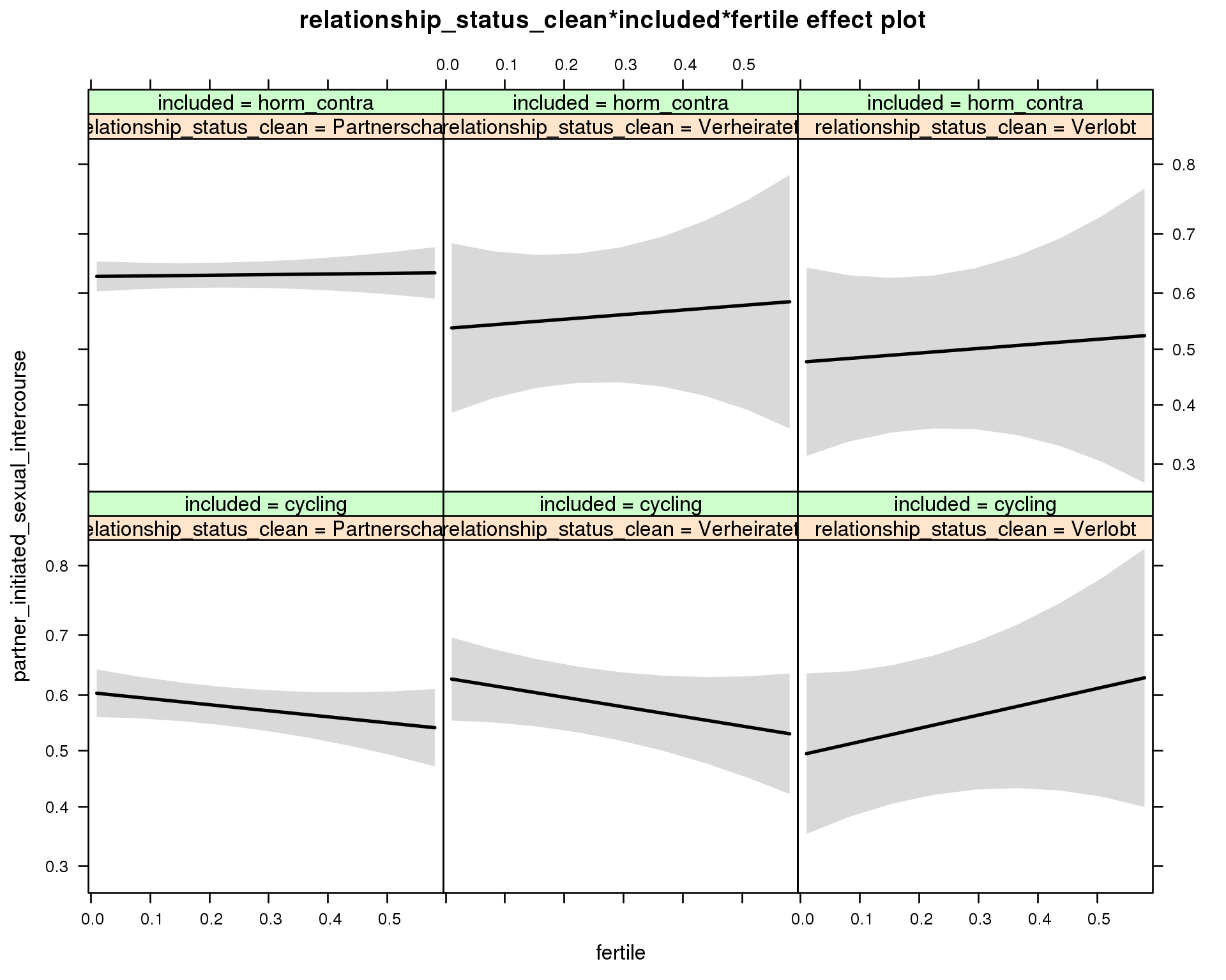
Generalized linear mixed model fit by maximum likelihood (Laplace Approximation) ['glmerMod']
Family: binomial ( probit )
Formula: partner_initiated_sexual_intercourse ~ menstruation + fertile_mean +
(1 | person) + relationship_status_clean + included + fertile +
menstruation:included + relationship_status_clean:included +
relationship_status_clean:fertile + included:fertile + relationship_status_clean:included:fertile
Data: diary
AIC BIC logLik deviance df.resid
7653 7773 -3809 7617 5730
Scaled residuals:
Min 1Q Median 3Q Max
-1.755 -1.112 0.657 0.779 1.337
Random effects:
Groups Name Variance Std.Dev.
person (Intercept) 0.0874 0.296
Number of obs: 5748, groups: person, 859
Fixed effects:
Estimate Std. Error z value Pr(>|z|)
(Intercept) 0.1467 0.0857 1.71 0.0871 .
menstruationpre 0.0398 0.0879 0.45 0.6504
menstruationyes 0.0738 0.0960 0.77 0.4420
fertile_mean 0.5864 0.3610 1.62 0.1043
relationship_status_cleanVerheiratet 0.0661 0.1109 0.60 0.5510
relationship_status_cleanVerlobt -0.2834 0.1959 -1.45 0.1479
includedhorm_contra 0.1227 0.0787 1.56 0.1189
fertile -0.2750 0.2027 -1.36 0.1750
menstruationpre:includedhorm_contra -0.1171 0.1088 -1.08 0.2817
menstruationyes:includedhorm_contra -0.3624 0.1264 -2.87 0.0041 **
relationship_status_cleanVerheiratet:includedhorm_contra -0.3023 0.2323 -1.30 0.1931
relationship_status_cleanVerlobt:includedhorm_contra -0.1061 0.2988 -0.36 0.7224
relationship_status_cleanVerheiratet:fertile -0.1616 0.3544 -0.46 0.6484
relationship_status_cleanVerlobt:fertile 0.8797 0.6539 1.34 0.1786
includedhorm_contra:fertile 0.3034 0.2395 1.27 0.2052
relationship_status_cleanVerheiratet:includedhorm_contra:fertile 0.3425 0.7773 0.44 0.6595
relationship_status_cleanVerlobt:includedhorm_contra:fertile -0.7005 1.0092 -0.69 0.4876
---
Signif. codes: 0 '***' 0.001 '**' 0.01 '*' 0.05 '.' 0.1 ' ' 1
convergence code: 0
Model failed to converge with max|grad| = 0.00469114 (tol = 0.001, component 1)
Satisfaction with sex
model_summaries$sexual_intercourse_satisfactionModel summary
Model summary
model %>%
print_summary()Linear mixed model fit by REML
t-tests use Satterthwaite approximations to degrees of freedom ['lmerMod']
Formula: sexual_intercourse_satisfaction ~ included * (menstruation +
fertile) + fertile_mean + (1 | person)
Data: diary
REML criterion at convergence: 14993
Scaled residuals:
Min 1Q Median 3Q Max
-5.125 -0.533 0.157 0.646 2.809
Random effects:
Groups Name Variance Std.Dev.
person (Intercept) 0.320 0.565
Residual 0.651 0.807
Number of obs: 5747, groups: person, 859
Fixed effects:
Estimate Std. Error df t value Pr(>|t|)
(Intercept) 5.05605 0.07543 1345.00000 67.03 <2e-16 ***
includedhorm_contra 0.08310 0.06138 1829.00000 1.35 0.18
menstruationpre -0.01815 0.05727 5428.00000 -0.32 0.75
menstruationyes -0.05805 0.06287 5436.00000 -0.92 0.36
fertile 0.06890 0.11519 5418.00000 0.60 0.55
fertile_mean -0.02938 0.34838 1187.00000 -0.08 0.93
includedhorm_contra:menstruationpre 0.04422 0.07074 5414.00000 0.63 0.53
includedhorm_contra:menstruationyes -0.00497 0.08281 5404.00000 -0.06 0.95
includedhorm_contra:fertile -0.23153 0.14137 5457.00000 -1.64 0.10
---
Signif. codes: 0 '***' 0.001 '**' 0.01 '*' 0.05 '.' 0.1 ' ' 1
Correlation of Fixed Effects:
(Intr) incld_ mnstrtnp mnstrtny fertil frtl_m inclddhrm_cntr:mnstrtnp
inclddhrm_c -0.493
menstrutnpr -0.295 0.372
menstrutnys -0.228 0.284 0.320
fertile -0.300 0.464 0.483 0.315
fertile_men -0.754 -0.050 -0.010 -0.003 -0.098
inclddhrm_cntr:mnstrtnp 0.249 -0.449 -0.809 -0.259 -0.389 -0.005
inclddhrm_cntr:mnstrtny 0.176 -0.323 -0.243 -0.759 -0.239 -0.002 0.295
inclddhrm_cntr:f 0.299 -0.562 -0.392 -0.257 -0.808 0.007 0.475
inclddhrm_cntr:mnstrtny
inclddhrm_c
menstrutnpr
menstrutnys
fertile
fertile_men
inclddhrm_cntr:mnstrtnp
inclddhrm_cntr:mnstrtny
inclddhrm_cntr:f 0.297
Effect size standardised by residual variance (\(\frac{b}{ SD_{residual} }\)): 0.09 [-0.19;0.37].
Marginal effect plots
model %>%
plot_all_effects()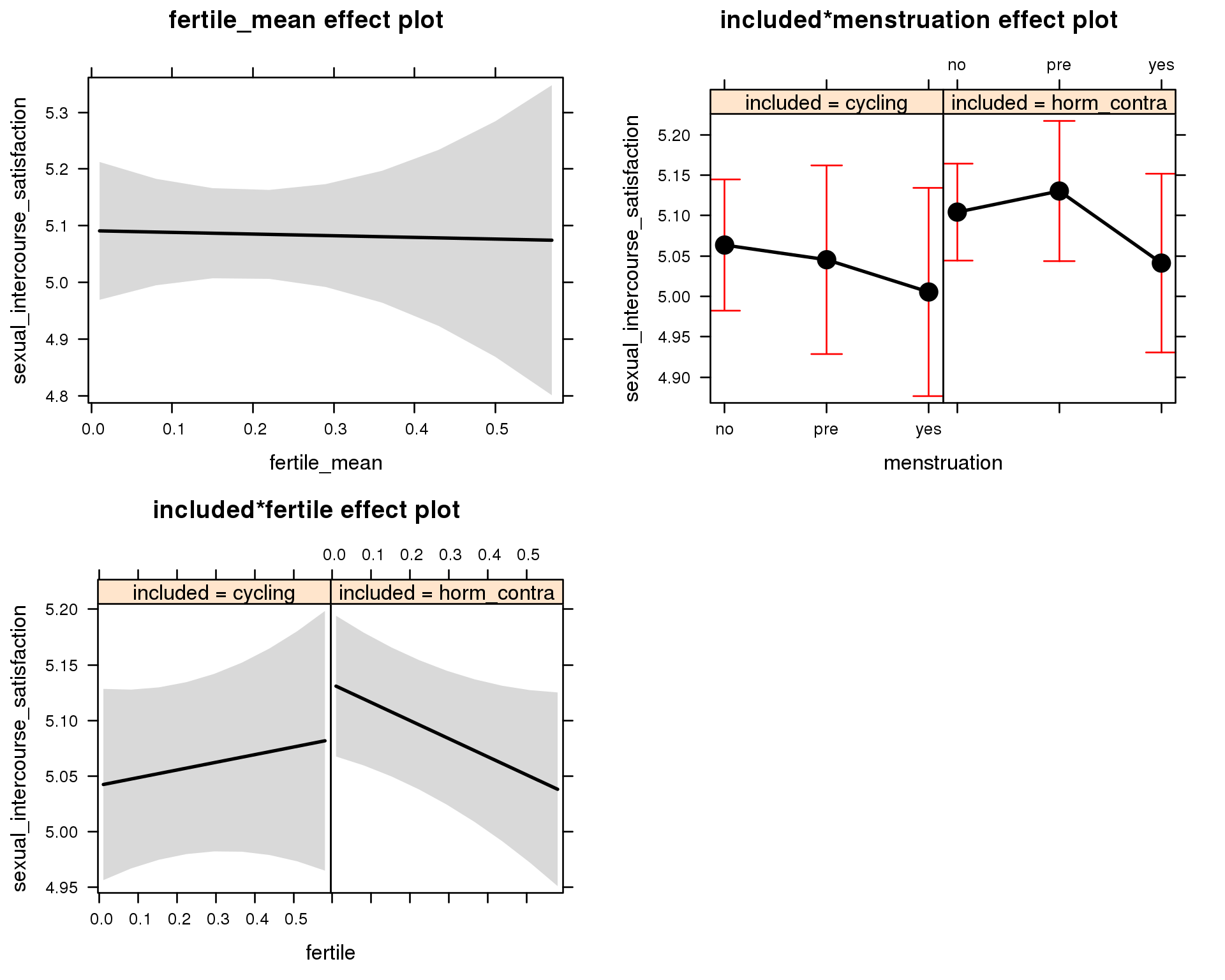
Outcome distribution
model %>%
plot_outcome(diary) + xlab(outcome_label)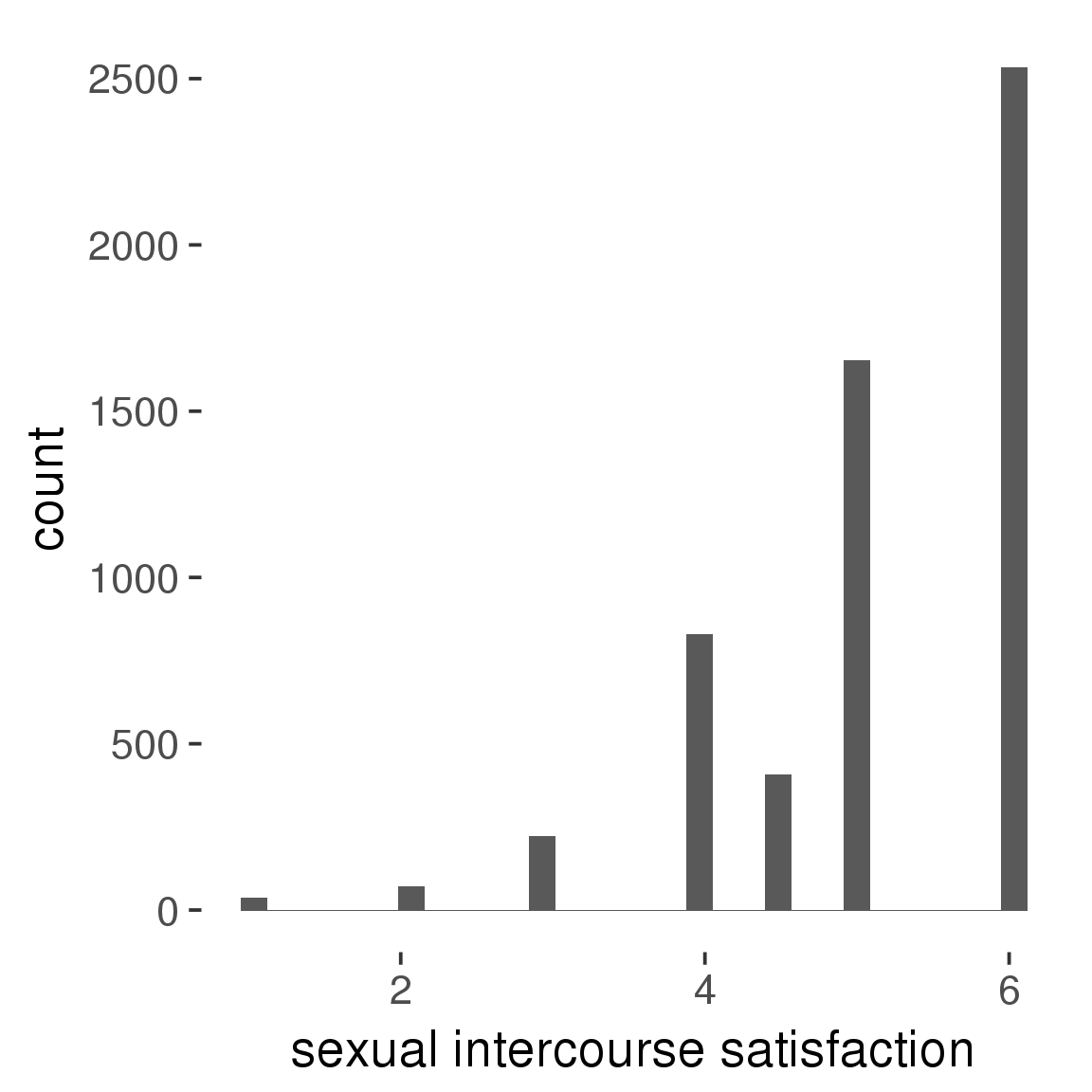
Diagnostics
model %>%
print_diagnostics()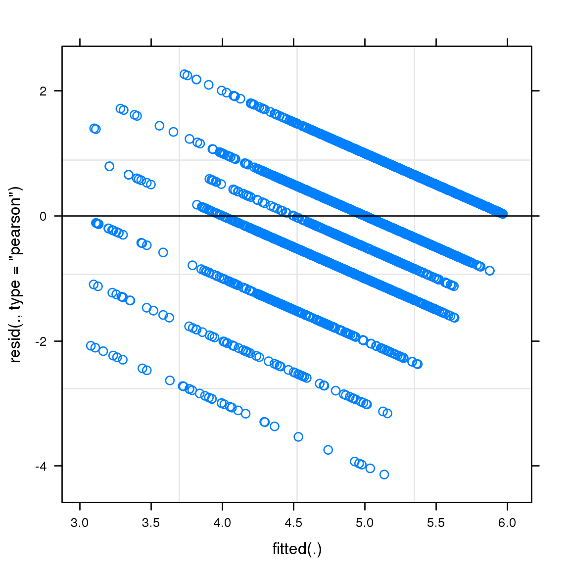
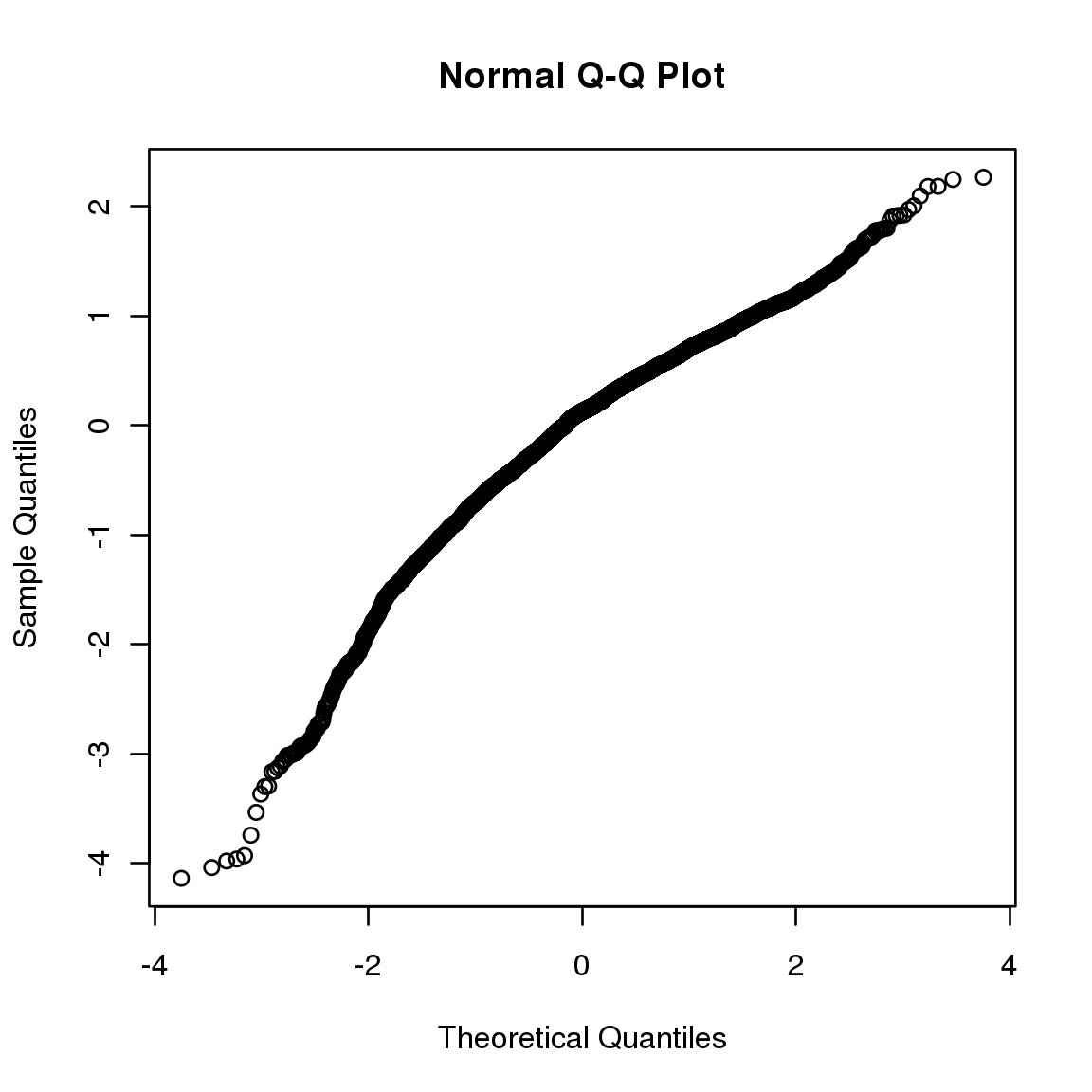
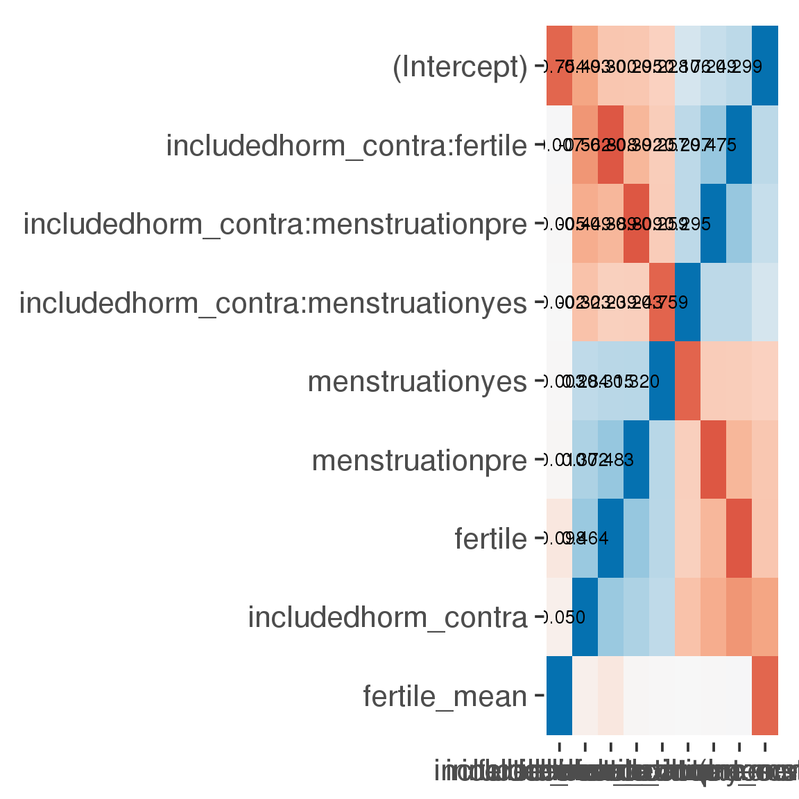
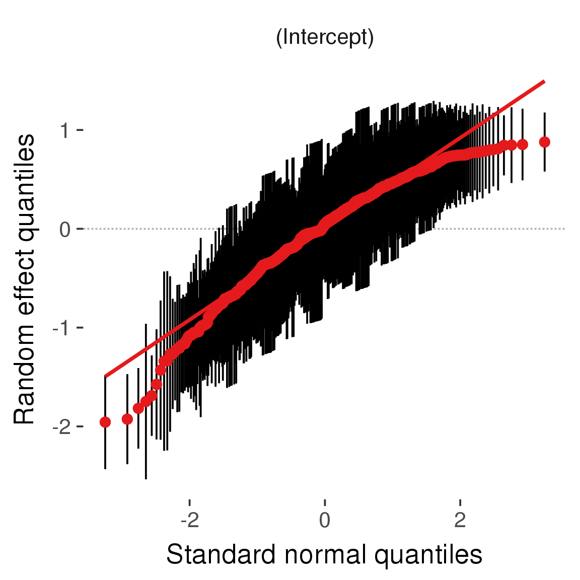
Curves
Here, we continuously plot the outcome over the course of the cycle. Because cycle lengths vary, we subset the data to cycles in a certain range. If the red curve traces the pink curve, our predictor accurately maps the relationship between fertile window probability and the outcome.
Cycle lengths from 21 to 36
Backward-counted
model %>%
plot_curve(diary %>% filter(minimum_cycle_length_diary <= 36, minimum_cycle_length_diary > 20) %>% mutate(fertile=prc_stirn_b))outcome = names(model@frame)[1]
outcome_label = recode(str_replace_all(str_replace_all(str_replace_all(outcome, "_", " "), " pair", "-pair"), " 1", ""),
"desirability 1" = "self-perceived desirability",
"NARQ admiration" = "narcissistic admiration",
"NARQ rivalry" = "narcissistic rivalry",
"extra-pair" = "extra-pair desire & behaviour",
"had sexual intercourse" = "sexual intercourse")
library(ggplot2)
# form a subset and run the model without the hormonal contraception and the fertility predictors
tmp = diary %>%
filter(!is.na(fertile), !is.na(included),
RCD > -1 * minimum_cycle_length_diary, RCD > -40)
new_form = update.formula(formula(model), new = . ~ . - fertile * included)
tmp$residuals = residuals(update(model, new_form, data = tmp , na.action = na.exclude))
tmp = tmp %>%
filter(!is.na(RCD), !is.na(residuals))
rcd_min = min(tmp$RCD)
tmp$real = FALSE
tmp_before = tmp
tmp_before$RCD = tmp_before$RCD + min(tmp$RCD) - 1
tmp_after = tmp
tmp_after$RCD = tmp_after$RCD - min(tmp$RCD) + 1
tmp$real = TRUE
tmp = bind_rows(tmp_before %>% filter(RCD > rcd_min - 11), tmp, tmp_after %>% filter(RCD < 11))GAM smooth on residuals
Here, we partialled out menstruation and individual random effects, then superimposed estimated probability of being in the fertile window scaled to the range of the estimated means. To address the periodicity of the cycle, we prepended and appended ten days of the timeseries to the end and the beginning of the timeseries. We then estimated the GAM and cut off the appended subsets before plotting.
tryCatch({
trend_plot = ggplot(tmp,aes(x = RCD, y = residuals, colour = included)) +
stat_smooth(geom = 'smooth',size = 0.8, fill = "#9ECAE1", method = 'gam', formula = y ~ s(x))
}, error = function(e){cat_message(e, "danger")})
tryCatch({
trend_data = ggplot_build(trend_plot)$data[[1]]
}, error = function(e){cat_message(e, "danger")})
trend_data$RCD = round(trend_data$x)
trend_data = left_join(trend_data, tmp %>% select(real, RCD,fertile) %>% unique(), by = "RCD")
trend_data %>%
filter(real == TRUE) %>%
mutate(superimposed = ( ( (fertile - 0.01)/0.58) * (max(y)-min(y) ) ) + min(y) ) ->
trend_data
ggplot(trend_data) +
geom_ribbon(aes(x = x, ymin = ymin, ymax = ymax, fill = factor(group)), alpha = 0.2) +
geom_line(aes(x = x, y = y, colour = factor(group)), size = 0.8, stat = "identity") +
scale_x_continuous(caption_x) +
geom_line(aes(x = x, y = superimposed), color = "#a83fbf", size = 1, linetype = 'dashed') +
annotate("text",x = mean(trend_data$x), y = max(trend_data$superimposed,na.rm=T) + 0.1, label = 'superimposed fertility peak', color = "#a83fbf") +
scale_y_continuous(outcome_label) +
ggtitle("GAM smooth, residuals") +
scale_color_manual("Contraception status",values = c("2"="black","1"= "red"), labels = c("2"="hormonally\ncontracepting","1"="cycling"), guide = F) +
scale_fill_manual("Contraception status",values = c("2"="black","1"= "red"), labels = c("2"="hormonally\ncontracepting","1"="cycling"), guide = F)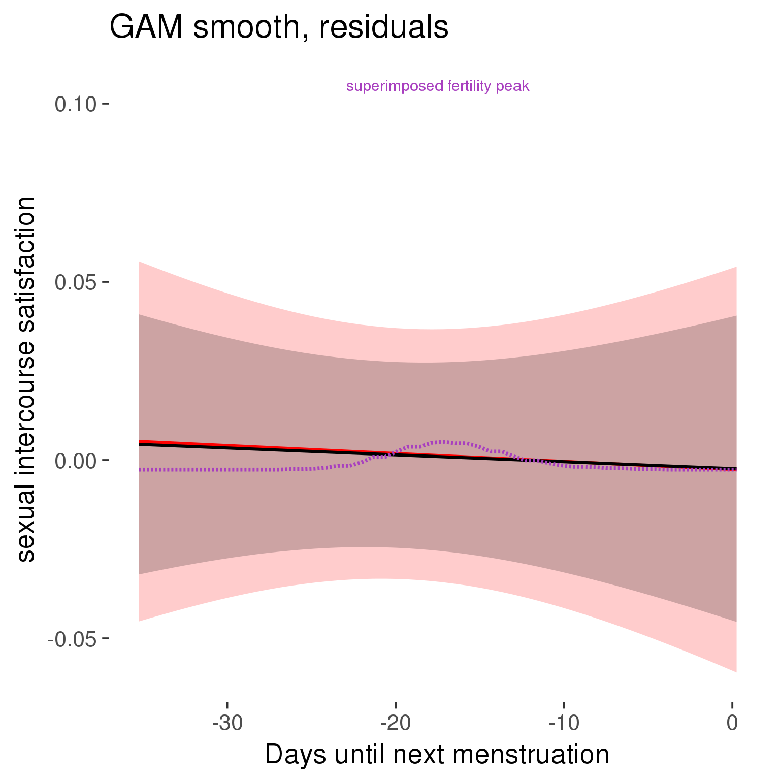
GAM smooth on raw data
As before, but without partialling anything out.
tryCatch({
trend_plot = ggplot(tmp,aes_string(x = "RCD", y = outcome, colour = "included")) +
stat_smooth(geom = 'smooth',size = 0.8, fill = "#9ECAE1", method = 'gam', formula = y ~ s(x))
}, error = function(e){cat_message(e, "danger")})
tryCatch({
trend_data = ggplot_build(trend_plot)$data[[1]]
}, error = function(e){cat_message(e, "danger")})
trend_data$RCD = round(trend_data$x)
trend_data = left_join(trend_data, tmp %>% select(real, RCD,fertile) %>% unique(), by = "RCD")
trend_data %>%
filter(real == TRUE) %>%
mutate(superimposed = ( ( (fertile - 0.01)/0.58) * (max(y)-min(y) ) ) + min(y) ) ->
trend_data
plot1b = ggplot(trend_data) +
geom_ribbon(aes(x = x, ymin = ymin, ymax = ymax, fill = factor(group)), alpha = 0.2) +
geom_line(aes(x = x, y = y, colour = factor(group)), size = 0.8, stat = "identity") +
scale_x_continuous(caption_x) +
geom_line(aes(x = x, y = superimposed), color = "#a83fbf", size = 1, linetype = 'dashed') +
annotate("text",x = mean(trend_data$x), y = max(trend_data$superimposed,na.rm=T) + 0.1, label = 'superimposed fertility peak', color = "#a83fbf") +
scale_y_continuous(outcome_label) +
ggtitle("GAM smooth, raw data") +
scale_color_manual("Contraception status",values = c("2"="black","1"= "red"), labels = c("2"="hormonally\ncontracepting","1"="cycling"), guide = F) +
scale_fill_manual("Contraception status",values = c("2"="black","1"= "red"), labels = c("2"="hormonally\ncontracepting","1"="cycling"), guide = F)
suppressWarnings(print(plot1b))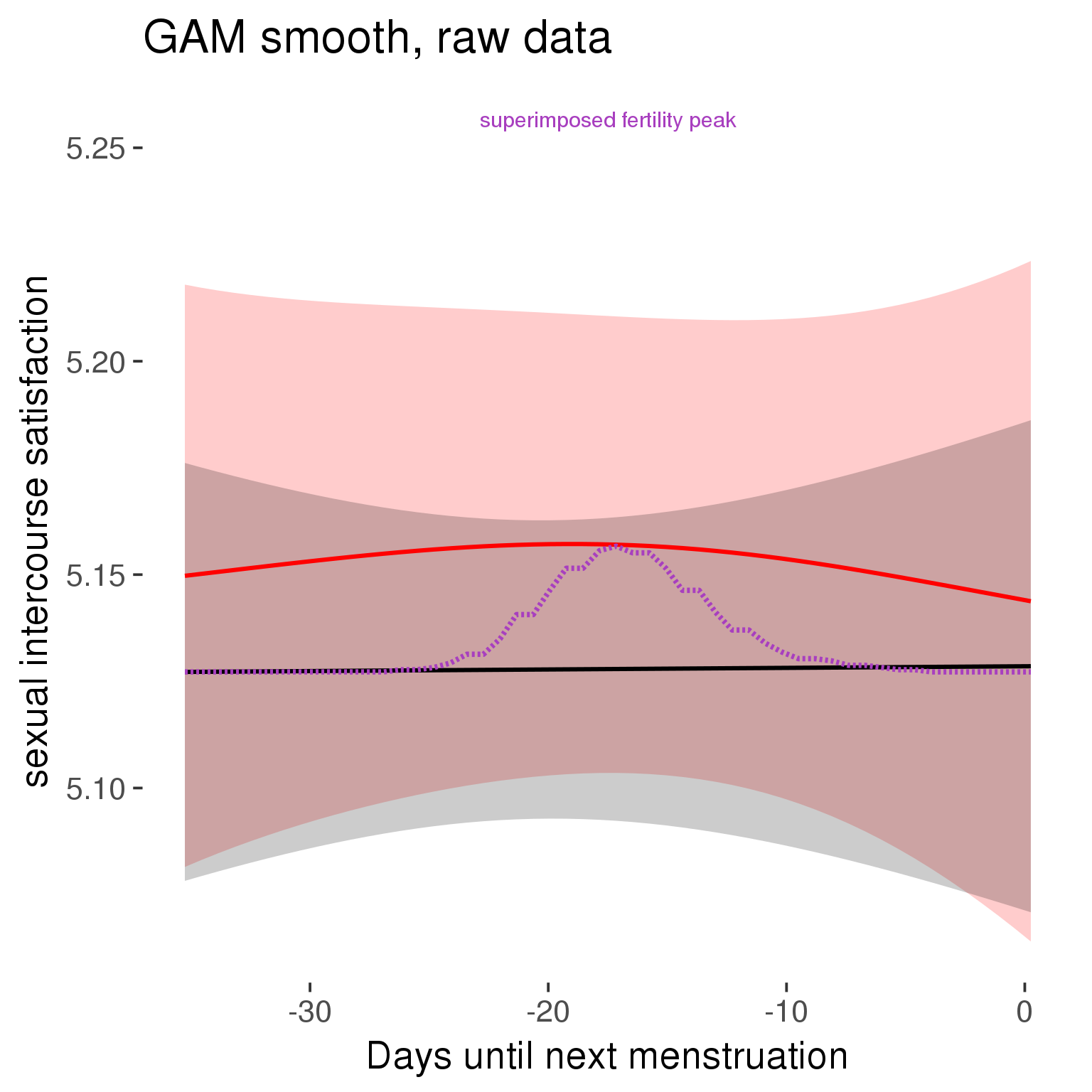
Means and standard errors over raw data
Nothing partialled out, just straight means with bootstrapped confidence intervals.
tryCatch({
trend_plot = ggplot(tmp,aes_string(x = "RCD", y = outcome, colour = "included")) +
geom_pointrange(size = 0.8, stat = 'summary', fun.data = "mean_cl_boot")
}, error = function(e){cat_message(e, "danger")})
tryCatch({
trend_data = ggplot_build(trend_plot)$data[[1]]
}, error = function(e){cat_message(e, "danger")})
trend_data$RCD = round(trend_data$x)
trend_data = left_join(trend_data, tmp %>% select(real, RCD,fertile) %>% unique(), by = "RCD")
trend_data %>%
filter(real == TRUE) %>%
mutate(superimposed = ( ( (fertile - 0.01)/0.58) * (max(y)-min(y) ) ) + min(y) ) ->
trend_data
plot3 = ggplot(trend_data) +
geom_pointrange(aes(x = x, y = y, ymin = ymin,ymax = ymax, colour = factor(group)), size = 0.8, stat = "identity", alpha = 0.6, position = position_dodge(width = .5)) +
scale_x_continuous("Days until next menstruation") +
geom_line(aes(x= x, y = superimposed), color = "#a83fbf", size = 1, linetype = 'dashed') +
annotate("text",x = mean(trend_data$x), y = max(trend_data$superimposed,na.rm=T) + 0.1, label = 'superimposed fertility peak', color = "#a83fbf") +
scale_y_continuous(outcome_label) +
ggtitle("Means with standard errors, raw data") +
scale_color_manual("Contraception status",values = c("2"="black","1"= "red"), labels = c("2"="hormonally\ncontracepting","1"="cycling"), guide = F) +
scale_fill_manual("Contraception status",values = c("2"="black","1"= "red"), labels = c("2"="hormonally\ncontracepting","1"="cycling"), guide = F)
suppressWarnings(print(plot3))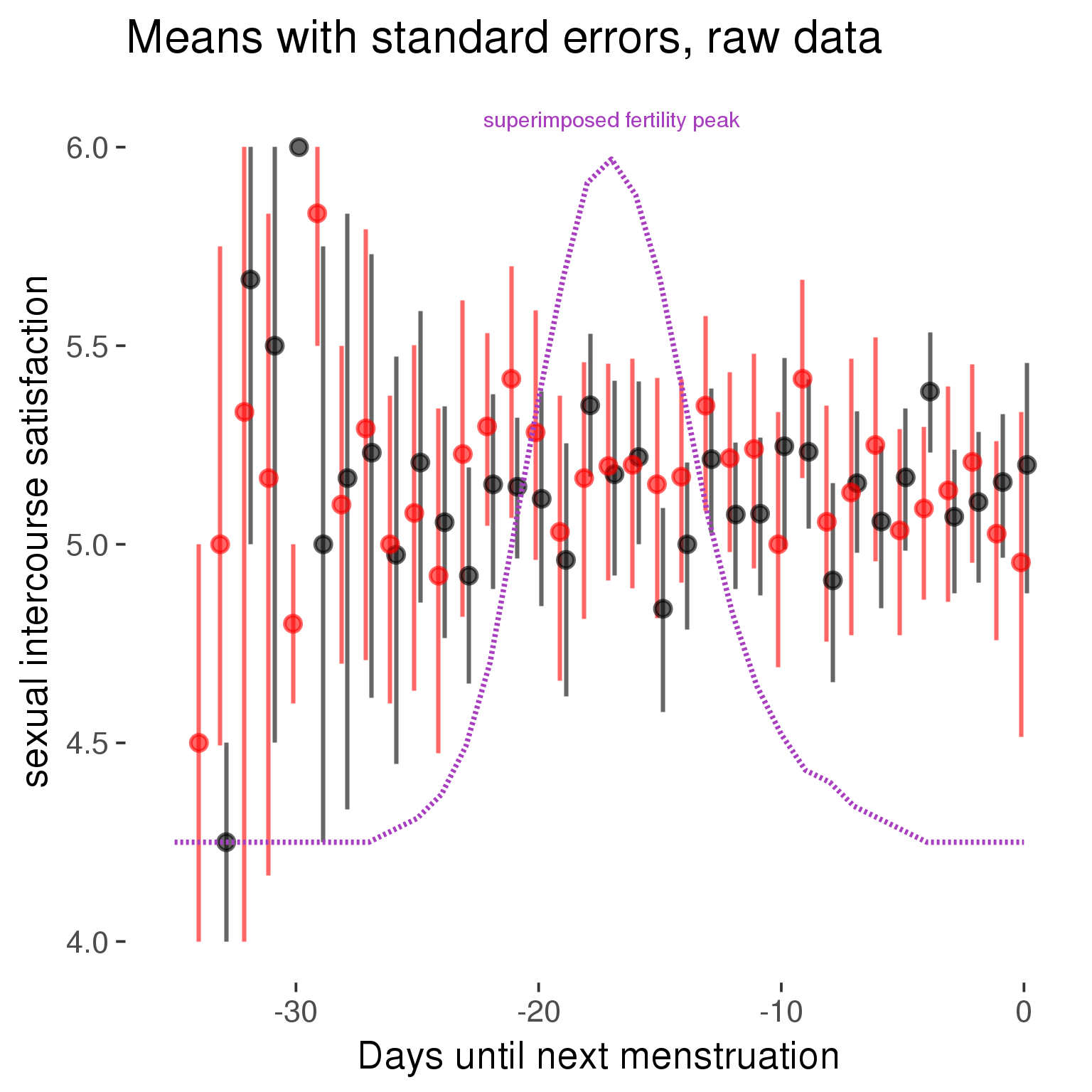
Forward-counted
model %>%
plot_curve(diary %>% filter(minimum_cycle_length_diary <= 36, minimum_cycle_length_diary > 20) %>% mutate(RCD = FCD, fertile = prc_stirn_b_forward_counted), caption_x = "Days since last menstruation")outcome = names(model@frame)[1]
outcome_label = recode(str_replace_all(str_replace_all(str_replace_all(outcome, "_", " "), " pair", "-pair"), " 1", ""),
"desirability 1" = "self-perceived desirability",
"NARQ admiration" = "narcissistic admiration",
"NARQ rivalry" = "narcissistic rivalry",
"extra-pair" = "extra-pair desire & behaviour",
"had sexual intercourse" = "sexual intercourse")
library(ggplot2)
# form a subset and run the model without the hormonal contraception and the fertility predictors
tmp = diary %>%
filter(!is.na(fertile), !is.na(included),
RCD > -1 * minimum_cycle_length_diary, RCD > -40)
new_form = update.formula(formula(model), new = . ~ . - fertile * included)
tmp$residuals = residuals(update(model, new_form, data = tmp , na.action = na.exclude))
tmp = tmp %>%
filter(!is.na(RCD), !is.na(residuals))
rcd_min = min(tmp$RCD)
tmp$real = FALSE
tmp_before = tmp
tmp_before$RCD = tmp_before$RCD + min(tmp$RCD) - 1
tmp_after = tmp
tmp_after$RCD = tmp_after$RCD - min(tmp$RCD) + 1
tmp$real = TRUE
tmp = bind_rows(tmp_before %>% filter(RCD > rcd_min - 11), tmp, tmp_after %>% filter(RCD < 11))GAM smooth on residuals
Here, we partialled out menstruation and individual random effects, then superimposed estimated probability of being in the fertile window scaled to the range of the estimated means. To address the periodicity of the cycle, we prepended and appended ten days of the timeseries to the end and the beginning of the timeseries. We then estimated the GAM and cut off the appended subsets before plotting.
tryCatch({
trend_plot = ggplot(tmp,aes(x = RCD, y = residuals, colour = included)) +
stat_smooth(geom = 'smooth',size = 0.8, fill = "#9ECAE1", method = 'gam', formula = y ~ s(x))
}, error = function(e){cat_message(e, "danger")})
tryCatch({
trend_data = ggplot_build(trend_plot)$data[[1]]
}, error = function(e){cat_message(e, "danger")})
trend_data$RCD = round(trend_data$x)
trend_data = left_join(trend_data, tmp %>% select(real, RCD,fertile) %>% unique(), by = "RCD")
trend_data %>%
filter(real == TRUE) %>%
mutate(superimposed = ( ( (fertile - 0.01)/0.58) * (max(y)-min(y) ) ) + min(y) ) ->
trend_data
ggplot(trend_data) +
geom_ribbon(aes(x = x, ymin = ymin, ymax = ymax, fill = factor(group)), alpha = 0.2) +
geom_line(aes(x = x, y = y, colour = factor(group)), size = 0.8, stat = "identity") +
scale_x_continuous(caption_x) +
geom_line(aes(x = x, y = superimposed), color = "#a83fbf", size = 1, linetype = 'dashed') +
annotate("text",x = mean(trend_data$x), y = max(trend_data$superimposed,na.rm=T) + 0.1, label = 'superimposed fertility peak', color = "#a83fbf") +
scale_y_continuous(outcome_label) +
ggtitle("GAM smooth, residuals") +
scale_color_manual("Contraception status",values = c("2"="black","1"= "red"), labels = c("2"="hormonally\ncontracepting","1"="cycling"), guide = F) +
scale_fill_manual("Contraception status",values = c("2"="black","1"= "red"), labels = c("2"="hormonally\ncontracepting","1"="cycling"), guide = F)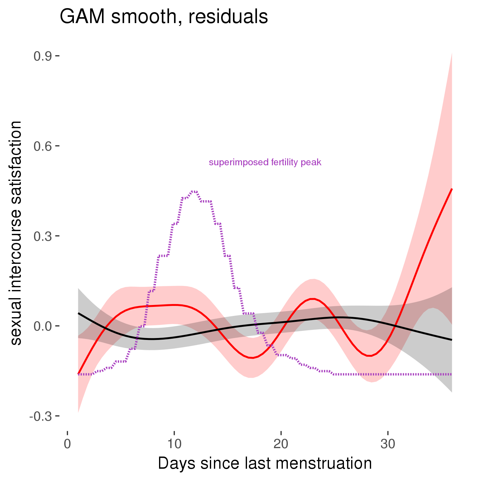
GAM smooth on raw data
As before, but without partialling anything out.
tryCatch({
trend_plot = ggplot(tmp,aes_string(x = "RCD", y = outcome, colour = "included")) +
stat_smooth(geom = 'smooth',size = 0.8, fill = "#9ECAE1", method = 'gam', formula = y ~ s(x))
}, error = function(e){cat_message(e, "danger")})
tryCatch({
trend_data = ggplot_build(trend_plot)$data[[1]]
}, error = function(e){cat_message(e, "danger")})
trend_data$RCD = round(trend_data$x)
trend_data = left_join(trend_data, tmp %>% select(real, RCD,fertile) %>% unique(), by = "RCD")
trend_data %>%
filter(real == TRUE) %>%
mutate(superimposed = ( ( (fertile - 0.01)/0.58) * (max(y)-min(y) ) ) + min(y) ) ->
trend_data
plot1b = ggplot(trend_data) +
geom_ribbon(aes(x = x, ymin = ymin, ymax = ymax, fill = factor(group)), alpha = 0.2) +
geom_line(aes(x = x, y = y, colour = factor(group)), size = 0.8, stat = "identity") +
scale_x_continuous(caption_x) +
geom_line(aes(x = x, y = superimposed), color = "#a83fbf", size = 1, linetype = 'dashed') +
annotate("text",x = mean(trend_data$x), y = max(trend_data$superimposed,na.rm=T) + 0.1, label = 'superimposed fertility peak', color = "#a83fbf") +
scale_y_continuous(outcome_label) +
ggtitle("GAM smooth, raw data") +
scale_color_manual("Contraception status",values = c("2"="black","1"= "red"), labels = c("2"="hormonally\ncontracepting","1"="cycling"), guide = F) +
scale_fill_manual("Contraception status",values = c("2"="black","1"= "red"), labels = c("2"="hormonally\ncontracepting","1"="cycling"), guide = F)
suppressWarnings(print(plot1b))
Means and standard errors over raw data
Nothing partialled out, just straight means with bootstrapped confidence intervals.
tryCatch({
trend_plot = ggplot(tmp,aes_string(x = "RCD", y = outcome, colour = "included")) +
geom_pointrange(size = 0.8, stat = 'summary', fun.data = "mean_cl_boot")
}, error = function(e){cat_message(e, "danger")})
tryCatch({
trend_data = ggplot_build(trend_plot)$data[[1]]
}, error = function(e){cat_message(e, "danger")})
trend_data$RCD = round(trend_data$x)
trend_data = left_join(trend_data, tmp %>% select(real, RCD,fertile) %>% unique(), by = "RCD")
trend_data %>%
filter(real == TRUE) %>%
mutate(superimposed = ( ( (fertile - 0.01)/0.58) * (max(y)-min(y) ) ) + min(y) ) ->
trend_data
plot3 = ggplot(trend_data) +
geom_pointrange(aes(x = x, y = y, ymin = ymin,ymax = ymax, colour = factor(group)), size = 0.8, stat = "identity", alpha = 0.6, position = position_dodge(width = .5)) +
scale_x_continuous("Days until next menstruation") +
geom_line(aes(x= x, y = superimposed), color = "#a83fbf", size = 1, linetype = 'dashed') +
annotate("text",x = mean(trend_data$x), y = max(trend_data$superimposed,na.rm=T) + 0.1, label = 'superimposed fertility peak', color = "#a83fbf") +
scale_y_continuous(outcome_label) +
ggtitle("Means with standard errors, raw data") +
scale_color_manual("Contraception status",values = c("2"="black","1"= "red"), labels = c("2"="hormonally\ncontracepting","1"="cycling"), guide = F) +
scale_fill_manual("Contraception status",values = c("2"="black","1"= "red"), labels = c("2"="hormonally\ncontracepting","1"="cycling"), guide = F)
suppressWarnings(print(plot3))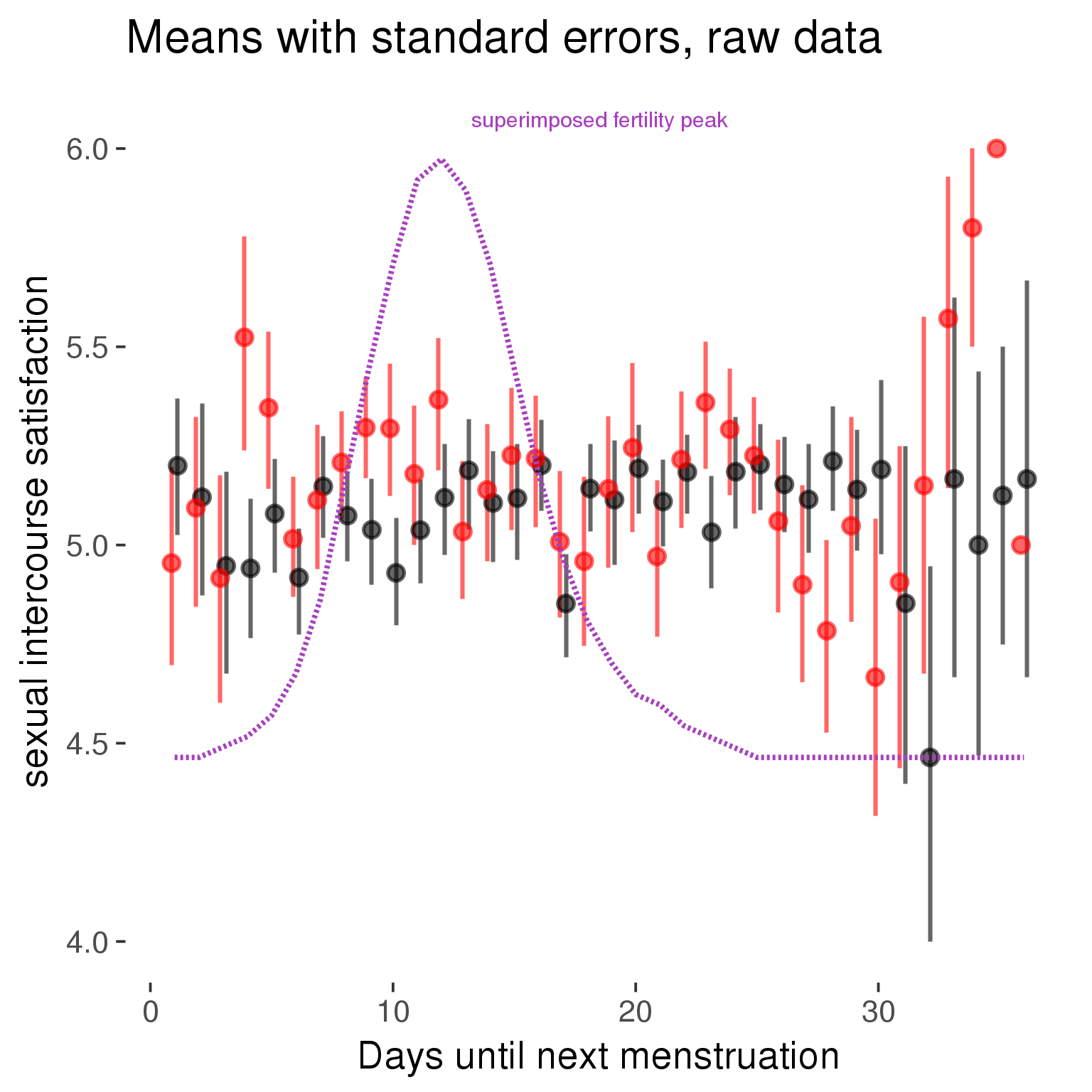
Cycle lengths from 27 to 30
Backward-counted
model %>%
plot_curve(diary %>% filter(minimum_cycle_length_diary <= 30, minimum_cycle_length_diary >= 27) %>% mutate(fertile=prc_stirn_b))outcome = names(model@frame)[1]
outcome_label = recode(str_replace_all(str_replace_all(str_replace_all(outcome, "_", " "), " pair", "-pair"), " 1", ""),
"desirability 1" = "self-perceived desirability",
"NARQ admiration" = "narcissistic admiration",
"NARQ rivalry" = "narcissistic rivalry",
"extra-pair" = "extra-pair desire & behaviour",
"had sexual intercourse" = "sexual intercourse")
library(ggplot2)
# form a subset and run the model without the hormonal contraception and the fertility predictors
tmp = diary %>%
filter(!is.na(fertile), !is.na(included),
RCD > -1 * minimum_cycle_length_diary, RCD > -40)
new_form = update.formula(formula(model), new = . ~ . - fertile * included)
tmp$residuals = residuals(update(model, new_form, data = tmp , na.action = na.exclude))
tmp = tmp %>%
filter(!is.na(RCD), !is.na(residuals))
rcd_min = min(tmp$RCD)
tmp$real = FALSE
tmp_before = tmp
tmp_before$RCD = tmp_before$RCD + min(tmp$RCD) - 1
tmp_after = tmp
tmp_after$RCD = tmp_after$RCD - min(tmp$RCD) + 1
tmp$real = TRUE
tmp = bind_rows(tmp_before %>% filter(RCD > rcd_min - 11), tmp, tmp_after %>% filter(RCD < 11))GAM smooth on residuals
Here, we partialled out menstruation and individual random effects, then superimposed estimated probability of being in the fertile window scaled to the range of the estimated means. To address the periodicity of the cycle, we prepended and appended ten days of the timeseries to the end and the beginning of the timeseries. We then estimated the GAM and cut off the appended subsets before plotting.
tryCatch({
trend_plot = ggplot(tmp,aes(x = RCD, y = residuals, colour = included)) +
stat_smooth(geom = 'smooth',size = 0.8, fill = "#9ECAE1", method = 'gam', formula = y ~ s(x))
}, error = function(e){cat_message(e, "danger")})
tryCatch({
trend_data = ggplot_build(trend_plot)$data[[1]]
}, error = function(e){cat_message(e, "danger")})
trend_data$RCD = round(trend_data$x)
trend_data = left_join(trend_data, tmp %>% select(real, RCD,fertile) %>% unique(), by = "RCD")
trend_data %>%
filter(real == TRUE) %>%
mutate(superimposed = ( ( (fertile - 0.01)/0.58) * (max(y)-min(y) ) ) + min(y) ) ->
trend_data
ggplot(trend_data) +
geom_ribbon(aes(x = x, ymin = ymin, ymax = ymax, fill = factor(group)), alpha = 0.2) +
geom_line(aes(x = x, y = y, colour = factor(group)), size = 0.8, stat = "identity") +
scale_x_continuous(caption_x) +
geom_line(aes(x = x, y = superimposed), color = "#a83fbf", size = 1, linetype = 'dashed') +
annotate("text",x = mean(trend_data$x), y = max(trend_data$superimposed,na.rm=T) + 0.1, label = 'superimposed fertility peak', color = "#a83fbf") +
scale_y_continuous(outcome_label) +
ggtitle("GAM smooth, residuals") +
scale_color_manual("Contraception status",values = c("2"="black","1"= "red"), labels = c("2"="hormonally\ncontracepting","1"="cycling"), guide = F) +
scale_fill_manual("Contraception status",values = c("2"="black","1"= "red"), labels = c("2"="hormonally\ncontracepting","1"="cycling"), guide = F)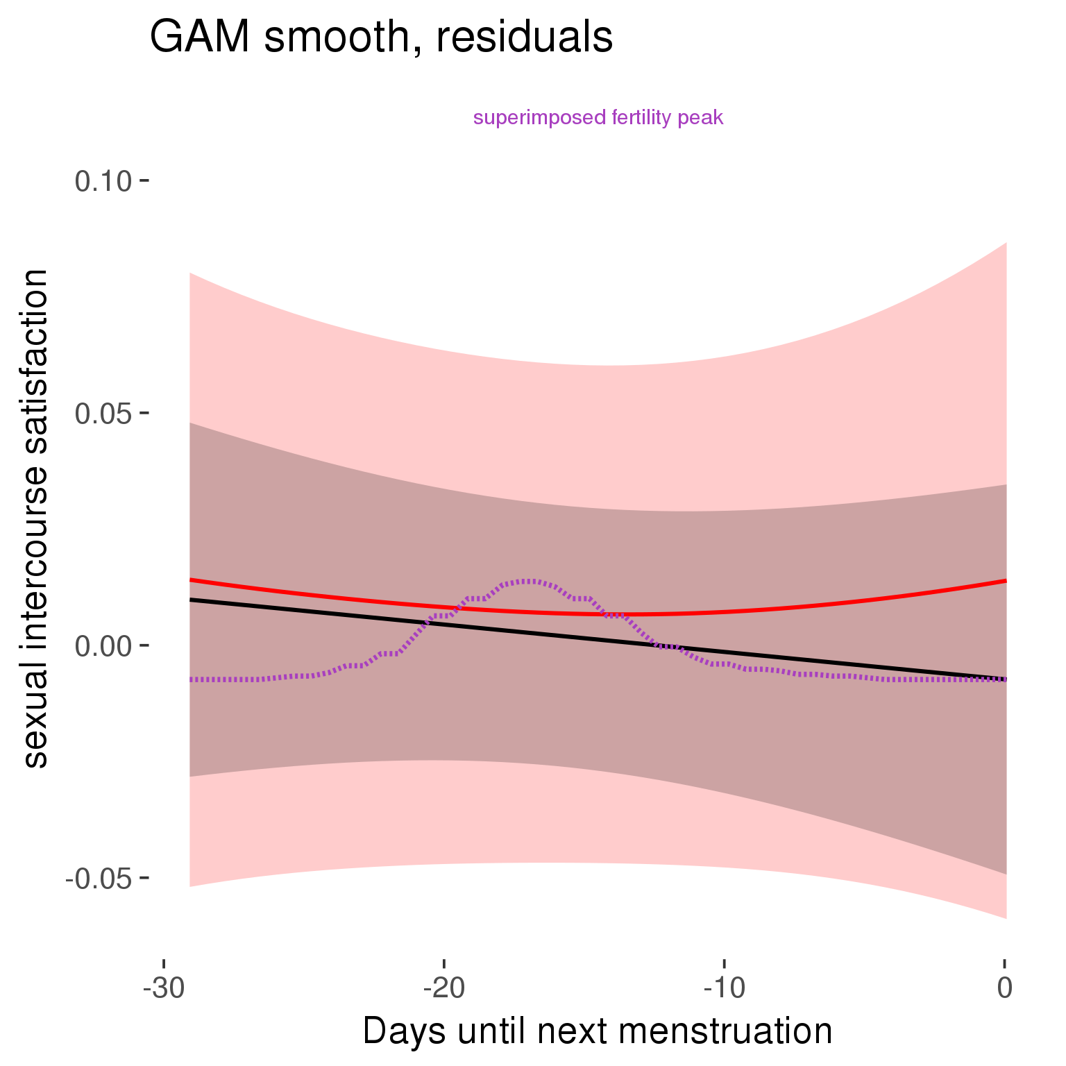
GAM smooth on raw data
As before, but without partialling anything out.
tryCatch({
trend_plot = ggplot(tmp,aes_string(x = "RCD", y = outcome, colour = "included")) +
stat_smooth(geom = 'smooth',size = 0.8, fill = "#9ECAE1", method = 'gam', formula = y ~ s(x))
}, error = function(e){cat_message(e, "danger")})
tryCatch({
trend_data = ggplot_build(trend_plot)$data[[1]]
}, error = function(e){cat_message(e, "danger")})
trend_data$RCD = round(trend_data$x)
trend_data = left_join(trend_data, tmp %>% select(real, RCD,fertile) %>% unique(), by = "RCD")
trend_data %>%
filter(real == TRUE) %>%
mutate(superimposed = ( ( (fertile - 0.01)/0.58) * (max(y)-min(y) ) ) + min(y) ) ->
trend_data
plot1b = ggplot(trend_data) +
geom_ribbon(aes(x = x, ymin = ymin, ymax = ymax, fill = factor(group)), alpha = 0.2) +
geom_line(aes(x = x, y = y, colour = factor(group)), size = 0.8, stat = "identity") +
scale_x_continuous(caption_x) +
geom_line(aes(x = x, y = superimposed), color = "#a83fbf", size = 1, linetype = 'dashed') +
annotate("text",x = mean(trend_data$x), y = max(trend_data$superimposed,na.rm=T) + 0.1, label = 'superimposed fertility peak', color = "#a83fbf") +
scale_y_continuous(outcome_label) +
ggtitle("GAM smooth, raw data") +
scale_color_manual("Contraception status",values = c("2"="black","1"= "red"), labels = c("2"="hormonally\ncontracepting","1"="cycling"), guide = F) +
scale_fill_manual("Contraception status",values = c("2"="black","1"= "red"), labels = c("2"="hormonally\ncontracepting","1"="cycling"), guide = F)
suppressWarnings(print(plot1b))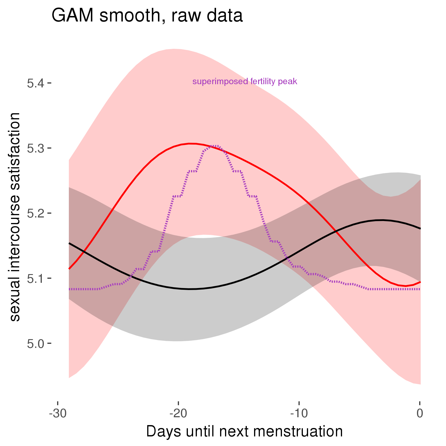
Means and standard errors over raw data
Nothing partialled out, just straight means with bootstrapped confidence intervals.
tryCatch({
trend_plot = ggplot(tmp,aes_string(x = "RCD", y = outcome, colour = "included")) +
geom_pointrange(size = 0.8, stat = 'summary', fun.data = "mean_cl_boot")
}, error = function(e){cat_message(e, "danger")})
tryCatch({
trend_data = ggplot_build(trend_plot)$data[[1]]
}, error = function(e){cat_message(e, "danger")})
trend_data$RCD = round(trend_data$x)
trend_data = left_join(trend_data, tmp %>% select(real, RCD,fertile) %>% unique(), by = "RCD")
trend_data %>%
filter(real == TRUE) %>%
mutate(superimposed = ( ( (fertile - 0.01)/0.58) * (max(y)-min(y) ) ) + min(y) ) ->
trend_data
plot3 = ggplot(trend_data) +
geom_pointrange(aes(x = x, y = y, ymin = ymin,ymax = ymax, colour = factor(group)), size = 0.8, stat = "identity", alpha = 0.6, position = position_dodge(width = .5)) +
scale_x_continuous("Days until next menstruation") +
geom_line(aes(x= x, y = superimposed), color = "#a83fbf", size = 1, linetype = 'dashed') +
annotate("text",x = mean(trend_data$x), y = max(trend_data$superimposed,na.rm=T) + 0.1, label = 'superimposed fertility peak', color = "#a83fbf") +
scale_y_continuous(outcome_label) +
ggtitle("Means with standard errors, raw data") +
scale_color_manual("Contraception status",values = c("2"="black","1"= "red"), labels = c("2"="hormonally\ncontracepting","1"="cycling"), guide = F) +
scale_fill_manual("Contraception status",values = c("2"="black","1"= "red"), labels = c("2"="hormonally\ncontracepting","1"="cycling"), guide = F)
suppressWarnings(print(plot3))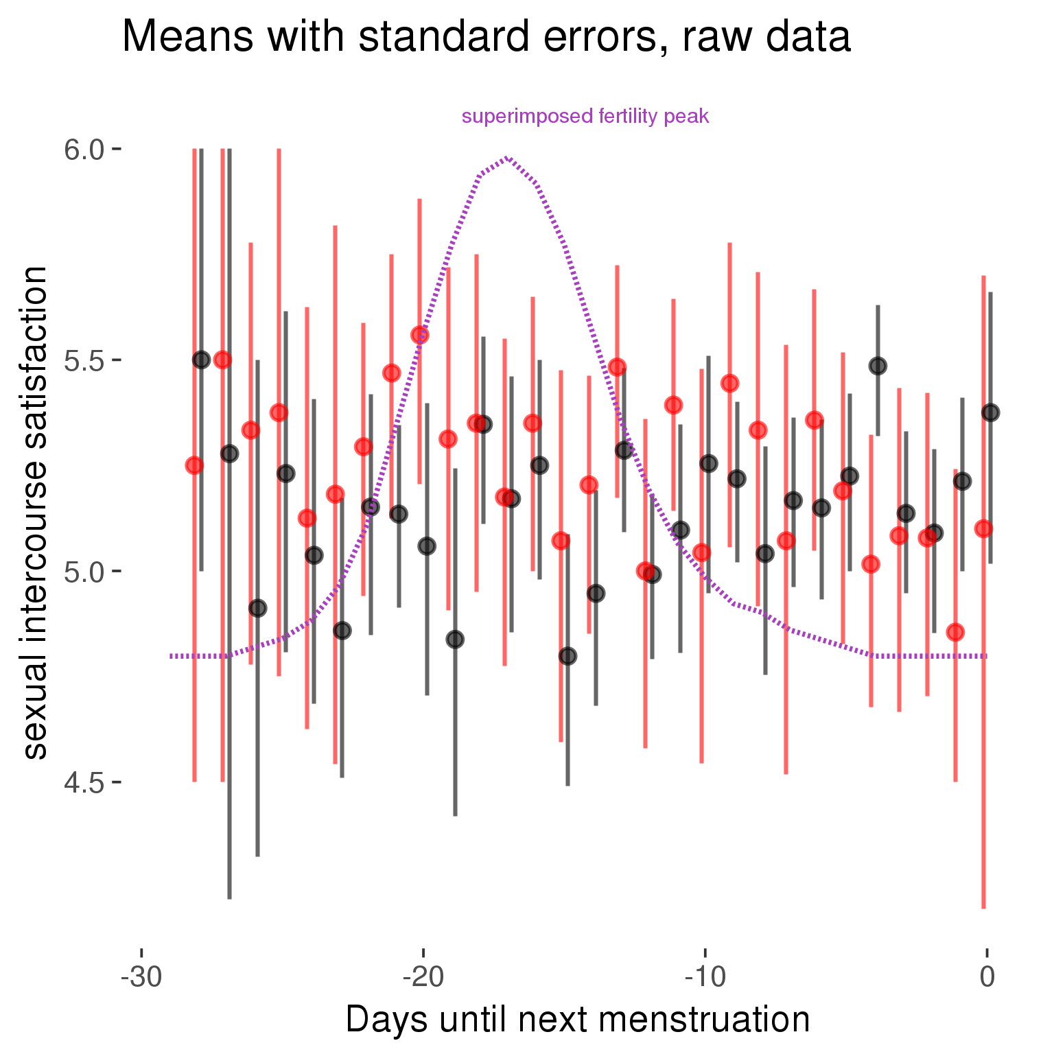
Forward-counted
model %>%
plot_curve(diary %>% filter(minimum_cycle_length_diary <= 30, minimum_cycle_length_diary >= 27) %>% mutate(RCD = FCD, fertile = prc_stirn_b_forward_counted), caption_x = "Days since last menstruation")outcome = names(model@frame)[1]
outcome_label = recode(str_replace_all(str_replace_all(str_replace_all(outcome, "_", " "), " pair", "-pair"), " 1", ""),
"desirability 1" = "self-perceived desirability",
"NARQ admiration" = "narcissistic admiration",
"NARQ rivalry" = "narcissistic rivalry",
"extra-pair" = "extra-pair desire & behaviour",
"had sexual intercourse" = "sexual intercourse")
library(ggplot2)
# form a subset and run the model without the hormonal contraception and the fertility predictors
tmp = diary %>%
filter(!is.na(fertile), !is.na(included),
RCD > -1 * minimum_cycle_length_diary, RCD > -40)
new_form = update.formula(formula(model), new = . ~ . - fertile * included)
tmp$residuals = residuals(update(model, new_form, data = tmp , na.action = na.exclude))
tmp = tmp %>%
filter(!is.na(RCD), !is.na(residuals))
rcd_min = min(tmp$RCD)
tmp$real = FALSE
tmp_before = tmp
tmp_before$RCD = tmp_before$RCD + min(tmp$RCD) - 1
tmp_after = tmp
tmp_after$RCD = tmp_after$RCD - min(tmp$RCD) + 1
tmp$real = TRUE
tmp = bind_rows(tmp_before %>% filter(RCD > rcd_min - 11), tmp, tmp_after %>% filter(RCD < 11))GAM smooth on residuals
Here, we partialled out menstruation and individual random effects, then superimposed estimated probability of being in the fertile window scaled to the range of the estimated means. To address the periodicity of the cycle, we prepended and appended ten days of the timeseries to the end and the beginning of the timeseries. We then estimated the GAM and cut off the appended subsets before plotting.
tryCatch({
trend_plot = ggplot(tmp,aes(x = RCD, y = residuals, colour = included)) +
stat_smooth(geom = 'smooth',size = 0.8, fill = "#9ECAE1", method = 'gam', formula = y ~ s(x))
}, error = function(e){cat_message(e, "danger")})
tryCatch({
trend_data = ggplot_build(trend_plot)$data[[1]]
}, error = function(e){cat_message(e, "danger")})
trend_data$RCD = round(trend_data$x)
trend_data = left_join(trend_data, tmp %>% select(real, RCD,fertile) %>% unique(), by = "RCD")
trend_data %>%
filter(real == TRUE) %>%
mutate(superimposed = ( ( (fertile - 0.01)/0.58) * (max(y)-min(y) ) ) + min(y) ) ->
trend_data
ggplot(trend_data) +
geom_ribbon(aes(x = x, ymin = ymin, ymax = ymax, fill = factor(group)), alpha = 0.2) +
geom_line(aes(x = x, y = y, colour = factor(group)), size = 0.8, stat = "identity") +
scale_x_continuous(caption_x) +
geom_line(aes(x = x, y = superimposed), color = "#a83fbf", size = 1, linetype = 'dashed') +
annotate("text",x = mean(trend_data$x), y = max(trend_data$superimposed,na.rm=T) + 0.1, label = 'superimposed fertility peak', color = "#a83fbf") +
scale_y_continuous(outcome_label) +
ggtitle("GAM smooth, residuals") +
scale_color_manual("Contraception status",values = c("2"="black","1"= "red"), labels = c("2"="hormonally\ncontracepting","1"="cycling"), guide = F) +
scale_fill_manual("Contraception status",values = c("2"="black","1"= "red"), labels = c("2"="hormonally\ncontracepting","1"="cycling"), guide = F)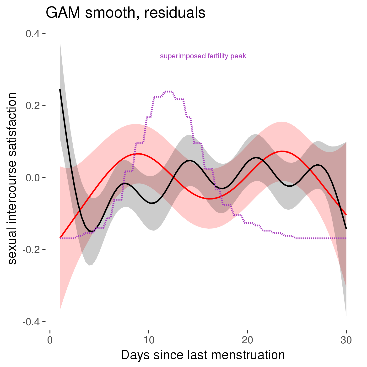
GAM smooth on raw data
As before, but without partialling anything out.
tryCatch({
trend_plot = ggplot(tmp,aes_string(x = "RCD", y = outcome, colour = "included")) +
stat_smooth(geom = 'smooth',size = 0.8, fill = "#9ECAE1", method = 'gam', formula = y ~ s(x))
}, error = function(e){cat_message(e, "danger")})
tryCatch({
trend_data = ggplot_build(trend_plot)$data[[1]]
}, error = function(e){cat_message(e, "danger")})
trend_data$RCD = round(trend_data$x)
trend_data = left_join(trend_data, tmp %>% select(real, RCD,fertile) %>% unique(), by = "RCD")
trend_data %>%
filter(real == TRUE) %>%
mutate(superimposed = ( ( (fertile - 0.01)/0.58) * (max(y)-min(y) ) ) + min(y) ) ->
trend_data
plot1b = ggplot(trend_data) +
geom_ribbon(aes(x = x, ymin = ymin, ymax = ymax, fill = factor(group)), alpha = 0.2) +
geom_line(aes(x = x, y = y, colour = factor(group)), size = 0.8, stat = "identity") +
scale_x_continuous(caption_x) +
geom_line(aes(x = x, y = superimposed), color = "#a83fbf", size = 1, linetype = 'dashed') +
annotate("text",x = mean(trend_data$x), y = max(trend_data$superimposed,na.rm=T) + 0.1, label = 'superimposed fertility peak', color = "#a83fbf") +
scale_y_continuous(outcome_label) +
ggtitle("GAM smooth, raw data") +
scale_color_manual("Contraception status",values = c("2"="black","1"= "red"), labels = c("2"="hormonally\ncontracepting","1"="cycling"), guide = F) +
scale_fill_manual("Contraception status",values = c("2"="black","1"= "red"), labels = c("2"="hormonally\ncontracepting","1"="cycling"), guide = F)
suppressWarnings(print(plot1b))
Means and standard errors over raw data
Nothing partialled out, just straight means with bootstrapped confidence intervals.
tryCatch({
trend_plot = ggplot(tmp,aes_string(x = "RCD", y = outcome, colour = "included")) +
geom_pointrange(size = 0.8, stat = 'summary', fun.data = "mean_cl_boot")
}, error = function(e){cat_message(e, "danger")})
tryCatch({
trend_data = ggplot_build(trend_plot)$data[[1]]
}, error = function(e){cat_message(e, "danger")})
trend_data$RCD = round(trend_data$x)
trend_data = left_join(trend_data, tmp %>% select(real, RCD,fertile) %>% unique(), by = "RCD")
trend_data %>%
filter(real == TRUE) %>%
mutate(superimposed = ( ( (fertile - 0.01)/0.58) * (max(y)-min(y) ) ) + min(y) ) ->
trend_data
plot3 = ggplot(trend_data) +
geom_pointrange(aes(x = x, y = y, ymin = ymin,ymax = ymax, colour = factor(group)), size = 0.8, stat = "identity", alpha = 0.6, position = position_dodge(width = .5)) +
scale_x_continuous("Days until next menstruation") +
geom_line(aes(x= x, y = superimposed), color = "#a83fbf", size = 1, linetype = 'dashed') +
annotate("text",x = mean(trend_data$x), y = max(trend_data$superimposed,na.rm=T) + 0.1, label = 'superimposed fertility peak', color = "#a83fbf") +
scale_y_continuous(outcome_label) +
ggtitle("Means with standard errors, raw data") +
scale_color_manual("Contraception status",values = c("2"="black","1"= "red"), labels = c("2"="hormonally\ncontracepting","1"="cycling"), guide = F) +
scale_fill_manual("Contraception status",values = c("2"="black","1"= "red"), labels = c("2"="hormonally\ncontracepting","1"="cycling"), guide = F)
suppressWarnings(print(plot3))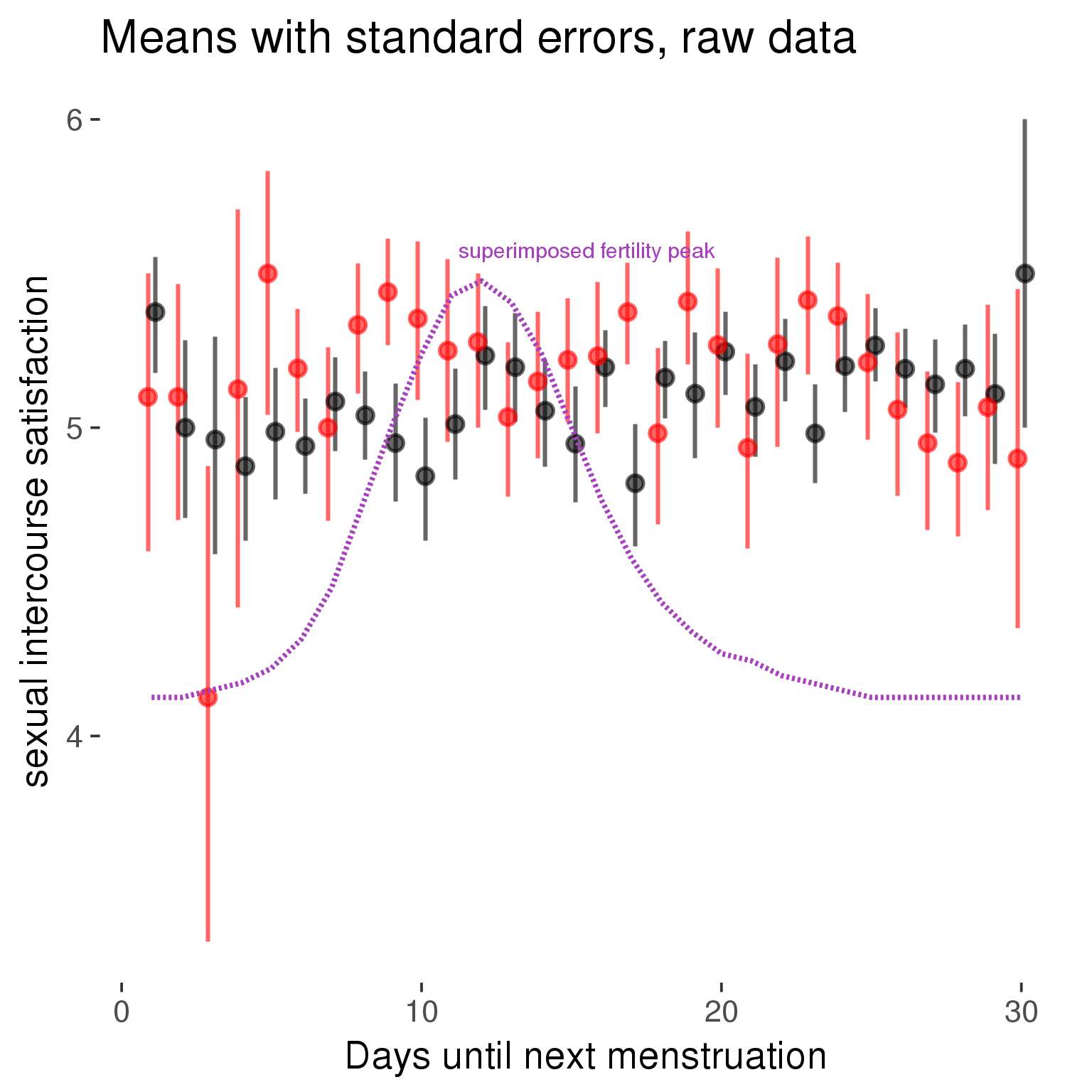
Robustness checks
M_r1: Random slopes for conception risk and menstruation
tryCatch({
# refit model with random effects for fertile and menstruation dummies
with_ind_diff = update(model, formula = . ~ . - (1| person) + (1 + fertile + menstruation | person))
# pull the random effects, format as tibble
rand = coef(with_ind_diff)$person %>%
tibble::rownames_to_column("person") %>%
mutate(person = as.numeric(person))
# pull the fixed effects
fixd = data.frame(fixef(with_ind_diff)) %>%
tibble::rownames_to_column("effect")
names(fixd) = c("effect", "pop_effect_size")
# pull apart the coefficients so that we can account for the fact that the random effect variation implicitly includes HC explaining the mean population-level effect of fertile/menstruation dummies among HC users
fixd = fixd %>%
separate(effect, c("included", "effect"), sep = ":", fill = "left") %>%
mutate(included = if_else(is.na(included), "cycling", str_replace(included, "included", "")))
fixd[2,c("included", "effect")] = c("horm_contra", "(Intercept)")
rand = rand %>%
# merge diary data on the random effects, so that we know who is a HC users and who isn't
inner_join(diary %>% select(person, included) %>% unique(), by = 'person') %>%
# gather into long format, to have the dataset by predictor
gather(effect, value, -person, -included) %>%
inner_join(fixd, by = c('effect', 'included')) %>%
# pull the fixed effects
mutate(
# only for those who are HC users, add the moderated population effect size for this effect (the random effects have the reference category mean)
value = if_else(included == "horm_contra", value + pop_effect_size, value),
effect = recode(effect, "includedhorm_contra" = "HC user",
"includedhorm_contra:fertile" = "HC user x fertile",
"includedhorm_contra:menstruationpre" = "HC user x premens.",
"includedhorm_contra:menstruationyes" = "HC user x mens.",
"menstruationyes" = "mens.",
"menstruationpre" = "premens.")) %>%
group_by(included, effect) %>%
# filter out predictors that aren't modelled as varying/random
filter(sd(value) > 0)
# plot dot plot of random effects
print(
ggplot(rand, aes(x = included, y = value, color = included, fill = included)) +
facet_wrap( ~ effect, scales = "free") +
# geom_violin(alpha = 0.4, size = 0) +
geom_dotplot(binaxis='y', dotsize = 0.1, method = "histodot") +
# geom_jitter(alpha = 0.05) +
coord_flip() +
geom_pointrange(stat = 'summary', fun.data = 'mean_sdl', color = 'darkred', size = 1.2) +
scale_color_manual("Contraception status", values = c("horm_contra"="black","cycling"= "red"), labels = c("horm_contra"="hormonally\ncontracepting","cycling"="cycling"), guide = F) +
scale_fill_manual("Contraception status", values = c("horm_contra"="black","cycling"= "red"), labels = c("horm_contra"="hormonally\ncontracepting","1"="cycling"), guide = F) +
ggtitle("M_r1: allowing participant-varying slopes", subtitle = "for the conception risk measure and the menstruation dummies") +
scale_x_discrete("Hormonal contraception", breaks = c("horm_contra", "cycling"), labels = c("yes", "no")) +
scale_y_continuous("Random effect size distribution"))
print_summary(with_ind_diff)
cat(pander(anova(model, with_ind_diff)))
}, error = function(e){
with_ind_diff = model
cat_message(e, "danger")
})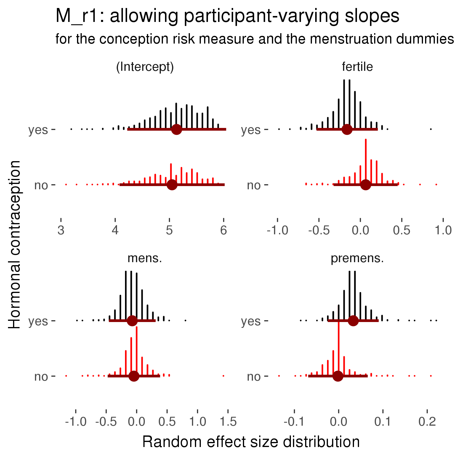
Linear mixed model fit by REML ['lmerMod']
Formula: sexual_intercourse_satisfaction ~ included + menstruation + fertile +
fertile_mean + (1 + fertile + menstruation | person) + included:menstruation + included:fertile
Data: diary
REML criterion at convergence: 14956
Scaled residuals:
Min 1Q Median 3Q Max
-5.051 -0.509 0.157 0.634 2.646
Random effects:
Groups Name Variance Std.Dev. Corr
person (Intercept) 0.3316 0.576
fertile 0.3234 0.569 -0.11
menstruationpre 0.0126 0.112 -0.06 0.29
menstruationyes 0.2405 0.490 -0.31 0.55 -0.59
Residual 0.6206 0.788
Number of obs: 5747, groups: person, 859
Fixed effects:
Estimate Std. Error t value
(Intercept) 5.04863 0.07595 66.5
includedhorm_contra 0.08407 0.06189 1.4
menstruationpre -0.00164 0.05740 0.0
menstruationyes -0.04475 0.07535 -0.6
fertile 0.06465 0.12214 0.5
fertile_mean -0.00109 0.35080 0.0
includedhorm_contra:menstruationpre 0.03466 0.07083 0.5
includedhorm_contra:menstruationyes -0.02735 0.09842 -0.3
includedhorm_contra:fertile -0.22512 0.14988 -1.5
Correlation of Fixed Effects:
(Intr) incld_ mnstrtnp mnstrtny fertil frtl_m inclddhrm_cntr:mnstrtnp
inclddhrm_c -0.495
menstrutnpr -0.293 0.370
menstrutnys -0.252 0.315 0.223
fertile -0.301 0.462 0.469 0.336
fertile_men -0.752 -0.050 -0.011 -0.005 -0.095
inclddhrm_cntr:mnstrtnp 0.247 -0.444 -0.810 -0.181 -0.378 -0.005
inclddhrm_cntr:mnstrtny 0.195 -0.361 -0.171 -0.766 -0.257 0.001 0.205
inclddhrm_cntr:f 0.298 -0.558 -0.381 -0.273 -0.808 0.007 0.460
inclddhrm_cntr:mnstrtny
inclddhrm_c
menstrutnpr
menstrutnys
fertile
fertile_men
inclddhrm_cntr:mnstrtnp
inclddhrm_cntr:mnstrtny
inclddhrm_cntr:f 0.315
refitting model(s) with ML (instead of REML)
| Df | AIC | BIC | logLik | deviance | Chisq | Chi Df | Pr(>Chisq) | |
|---|---|---|---|---|---|---|---|---|
| object | 11 | 14983 | 15056 | -7480 | 14961 | NA | NA | NA |
| ..1 | 20 | 14964 | 15097 | -7462 | 14924 | 36.63 | 9 | 0.00003061 |
robustness_check_ovu_shift(model, diary)M_e: Exclusion criteria
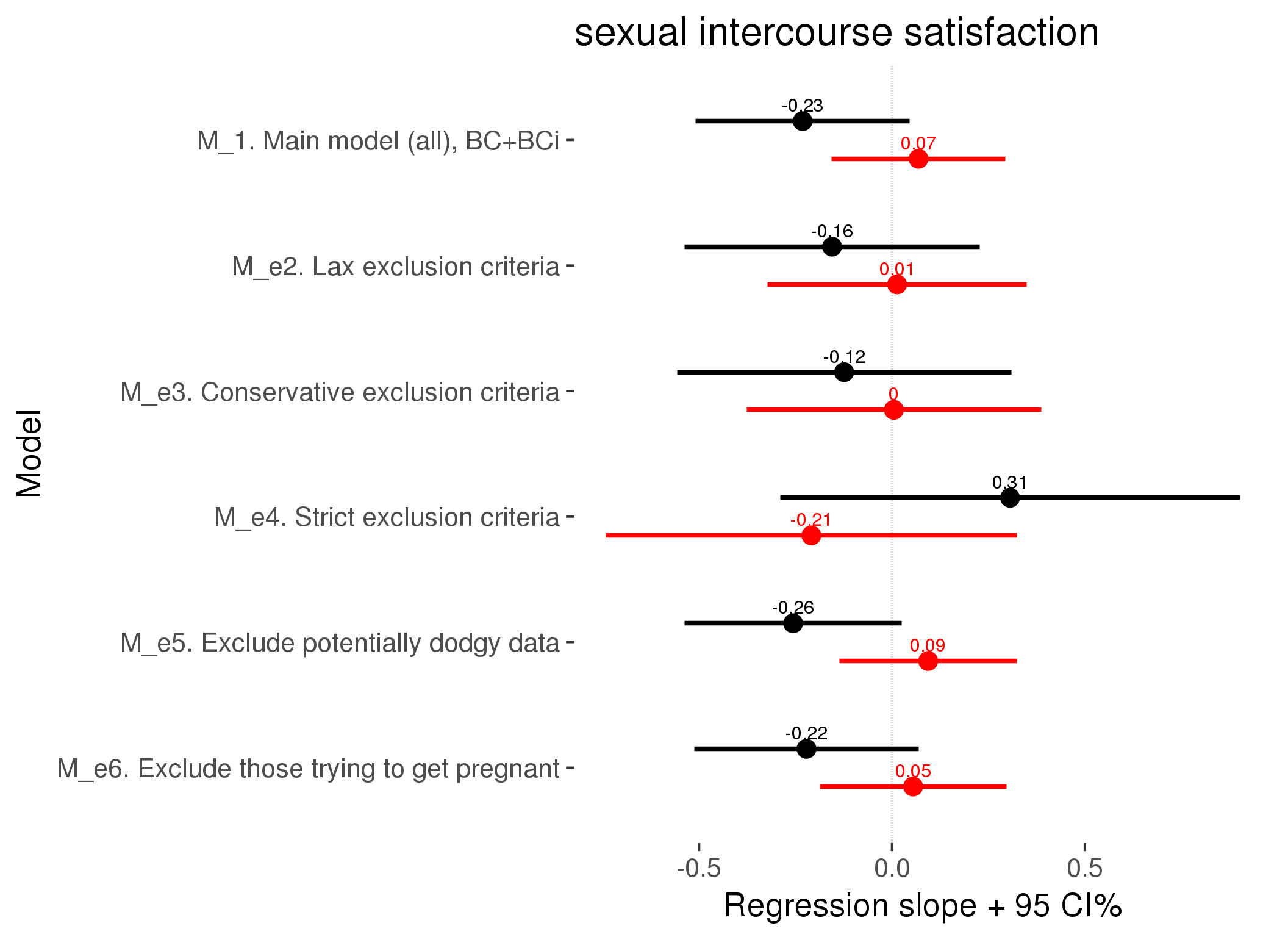
M_p: Predictors
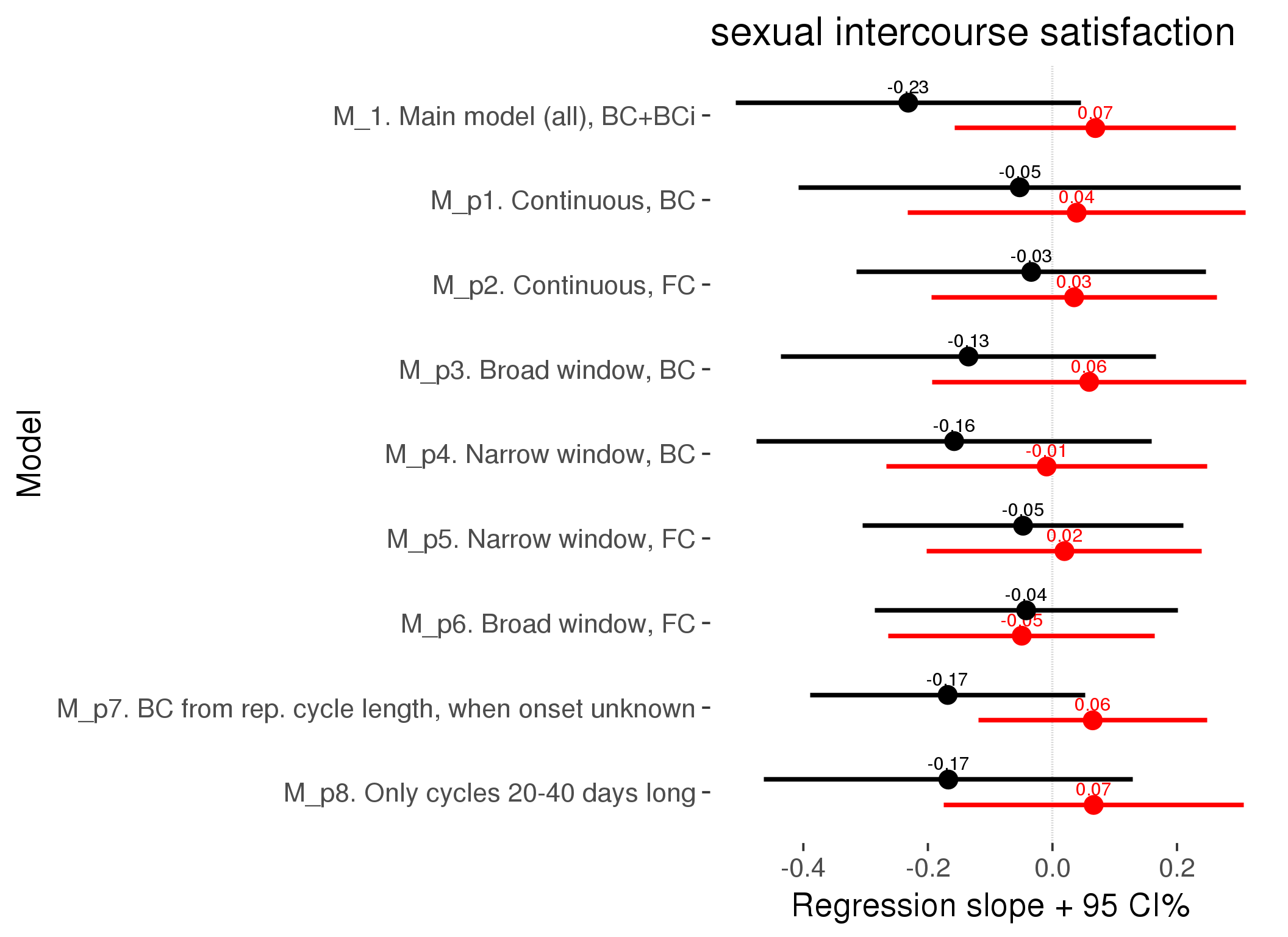
M_c: Covariates, controls, autocorrelation
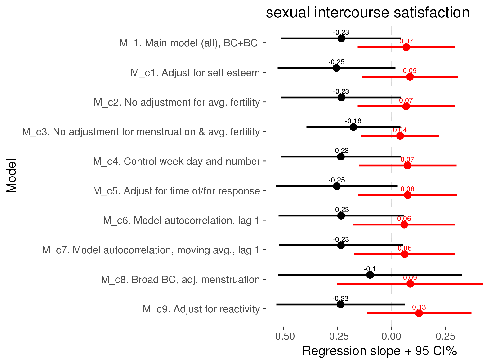
Linear mixed model fit by REML ['lmerMod']
REML criterion at convergence: 13177
Scaled residuals:
Min 1Q Median 3Q Max
-5.207 -0.536 0.158 0.646 3.217
Random effects:
Groups Name Variance Std.Dev.
person (Intercept) 3.25e-01 0.569663117
Xr.2 s(days_filled_out):includedhorm_contra 0.00e+00 0.000000000
Xr.1 s(days_filled_out):includedcycling 8.86e-14 0.000000298
Xr.0 s(day_number):includedhorm_contra 3.90e-04 0.019750380
Xr s(day_number):includedcycling 0.00e+00 0.000000000
Residual 6.29e-01 0.792886675
Number of obs: 5084, groups: person, 843; Xr.2, 8; Xr.1, 8; Xr.0, 8; Xr, 8
Fixed effects:
Estimate Std. Error t value
X(Intercept) 5.05635 0.07793 64.9
Xincludedhorm_contra 0.09256 0.06451 1.4
Xmenstruationpre -0.00464 0.05965 -0.1
Xmenstruationyes 0.02330 0.06822 0.3
Xfertile 0.12797 0.12356 1.0
Xfertile_mean -0.13533 0.35518 -0.4
Xincludedhorm_contra:menstruationpre 0.03656 0.07371 0.5
Xincludedhorm_contra:menstruationyes -0.02666 0.08958 -0.3
Xincludedhorm_contra:fertile -0.23492 0.15154 -1.6
Xs(day_number):includedcyclingFx1 0.04794 0.07918 0.6
Xs(day_number):includedhorm_contraFx1 0.01455 0.05994 0.2
Xs(days_filled_out):includedcyclingFx1 -0.04494 0.08130 -0.6
Xs(days_filled_out):includedhorm_contraFx1 -0.00151 0.06076 0.0
Family: gaussian
Link function: identity
Formula:
sexual_intercourse_satisfaction ~ included + menstruation + fertile +
fertile_mean + s(day_number, by = included) + s(days_filled_out,
by = included) + included:menstruation + included:fertile
Parametric coefficients:
Estimate Std. Error t value Pr(>|t|)
(Intercept) 5.05635 0.07793 64.88 <2e-16 ***
includedhorm_contra 0.09256 0.06451 1.43 0.15
menstruationpre -0.00464 0.05965 -0.08 0.94
menstruationyes 0.02330 0.06822 0.34 0.73
fertile 0.12797 0.12356 1.04 0.30
fertile_mean -0.13533 0.35518 -0.38 0.70
includedhorm_contra:menstruationpre 0.03656 0.07371 0.50 0.62
includedhorm_contra:menstruationyes -0.02666 0.08958 -0.30 0.77
includedhorm_contra:fertile -0.23492 0.15154 -1.55 0.12
---
Signif. codes: 0 '***' 0.001 '**' 0.01 '*' 0.05 '.' 0.1 ' ' 1
Approximate significance of smooth terms:
edf Ref.df F p-value
s(day_number):includedcycling 1.00 1.00 0.37 0.54
s(day_number):includedhorm_contra 1.08 1.08 0.03 0.84
s(days_filled_out):includedcycling 1.00 1.00 0.31 0.58
s(days_filled_out):includedhorm_contra 1.00 1.00 0.00 0.98
R-sq.(adj) = -0.00228
lmer.REML = 13177 Scale est. = 0.62867 n = 5084
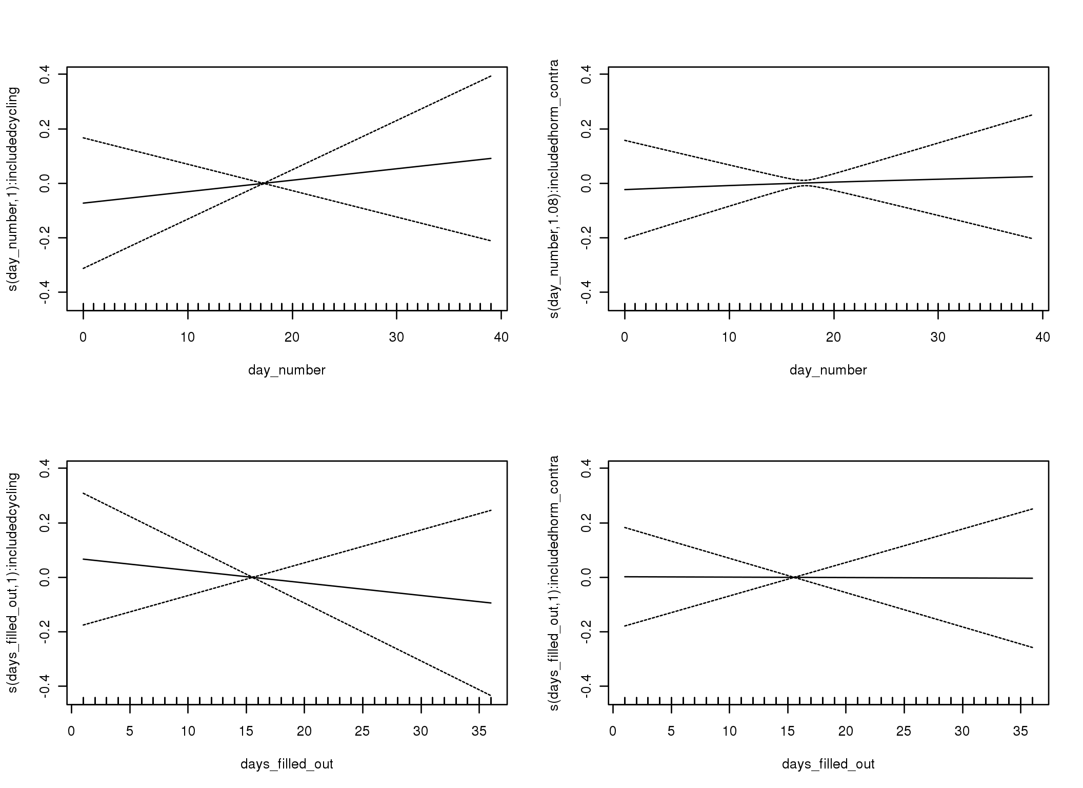
Linear mixed-effects model fit by REML
Data: diary
AIC BIC logLik
14976 15056 -7476
Random effects:
Formula: ~1 | person
(Intercept) Residual
StdDev: 0.5572 0.8135
Correlation Structure: ARMA(1,0)
Formula: ~day_number | person
Parameter estimate(s):
Phi1
0.1942
Fixed effects: sexual_intercourse_satisfaction ~ included * (menstruation + fertile) + fertile_mean
Value Std.Error DF t-value p-value
(Intercept) 5.048 0.0760 4882 66.39 0.0000
includedhorm_contra 0.085 0.0623 856 1.37 0.1710
menstruationpre -0.013 0.0594 4882 -0.21 0.8318
menstruationyes -0.058 0.0650 4882 -0.89 0.3722
fertile 0.059 0.1204 4882 0.49 0.6224
fertile_mean 0.007 0.3500 856 0.02 0.9831
includedhorm_contra:menstruationpre 0.029 0.0734 4882 0.39 0.6969
includedhorm_contra:menstruationyes -0.006 0.0852 4882 -0.07 0.9461
includedhorm_contra:fertile -0.233 0.1476 4882 -1.58 0.1153
Correlation:
(Intr) incld_ mnstrtnp mnstrtny fertil frtl_m inclddhrm_cntr:mnstrtnp
includedhorm_contra -0.498
menstruationpre -0.302 0.378
menstruationyes -0.237 0.291 0.323
fertile -0.307 0.473 0.473 0.311
fertile_mean -0.750 -0.049 -0.010 -0.002 -0.102
includedhorm_contra:menstruationpre 0.254 -0.457 -0.809 -0.261 -0.382 -0.005
includedhorm_contra:menstruationyes 0.183 -0.332 -0.246 -0.763 -0.237 -0.002 0.298
includedhorm_contra:fertile 0.307 -0.575 -0.385 -0.253 -0.808 0.009 0.467
inclddhrm_cntr:mnstrtny
includedhorm_contra
menstruationpre
menstruationyes
fertile
fertile_mean
includedhorm_contra:menstruationpre
includedhorm_contra:menstruationyes
includedhorm_contra:fertile 0.294
Standardized Within-Group Residuals:
Min Q1 Med Q3 Max
-5.1235 -0.5310 0.1687 0.6519 2.7107
Number of Observations: 5747
Number of Groups: 859
Linear mixed-effects model fit by REML
Data: diary
AIC BIC logLik
14977 15064 -7476
Random effects:
Formula: ~1 | person
(Intercept) Residual
StdDev: 0.558 0.8127
Correlation Structure: ARMA(1,1)
Formula: ~day_number | person
Parameter estimate(s):
Phi1 Theta1
0.01951 0.18271
Fixed effects: sexual_intercourse_satisfaction ~ included * (menstruation + fertile) + fertile_mean
Value Std.Error DF t-value p-value
(Intercept) 5.049 0.0760 4882 66.48 0.0000
includedhorm_contra 0.085 0.0622 856 1.37 0.1709
menstruationpre -0.014 0.0592 4882 -0.23 0.8194
menstruationyes -0.058 0.0648 4882 -0.89 0.3722
fertile 0.061 0.1198 4882 0.51 0.6084
fertile_mean 0.003 0.3497 856 0.01 0.9929
includedhorm_contra:menstruationpre 0.029 0.0732 4882 0.40 0.6887
includedhorm_contra:menstruationyes -0.004 0.0850 4882 -0.05 0.9602
includedhorm_contra:fertile -0.233 0.1469 4882 -1.59 0.1126
Correlation:
(Intr) incld_ mnstrtnp mnstrtny fertil frtl_m inclddhrm_cntr:mnstrtnp
includedhorm_contra -0.497
menstruationpre -0.302 0.378
menstruationyes -0.236 0.290 0.322
fertile -0.307 0.473 0.475 0.312
fertile_mean -0.750 -0.049 -0.010 -0.002 -0.102
includedhorm_contra:menstruationpre 0.254 -0.456 -0.809 -0.261 -0.383 -0.005
includedhorm_contra:menstruationyes 0.183 -0.332 -0.245 -0.762 -0.237 -0.002 0.297
includedhorm_contra:fertile 0.306 -0.574 -0.386 -0.254 -0.808 0.008 0.469
inclddhrm_cntr:mnstrtny
includedhorm_contra
menstruationpre
menstruationyes
fertile
fertile_mean
includedhorm_contra:menstruationpre
includedhorm_contra:menstruationyes
includedhorm_contra:fertile 0.295
Standardized Within-Group Residuals:
Min Q1 Med Q3 Max
-5.1180 -0.5290 0.1679 0.6521 2.7205
Number of Observations: 5747
Number of Groups: 859
M_d: Other designs
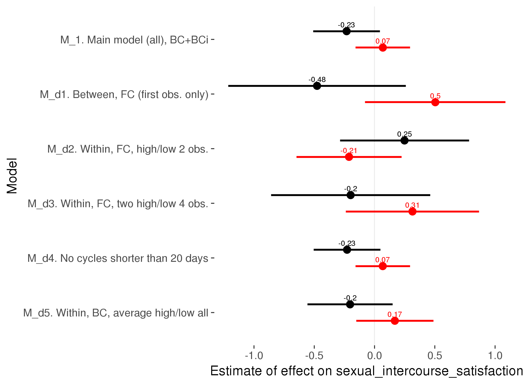
M_m1: Moderation by contraceptive method
Based on the sample with lax exclusion criteria. Users who used any hormonal contraception are classified as hormonal, users who use any awareness-based methods (counting, temperature-based) are classified as ‘fertility-awareness’, women who don’t fall into the before groups and use condoms, pessars, coitus interruptus etc. are classified as ‘barrie or abstinence’. Women who don’t use contraception or use other methods such as sterilisation are excluded from this analysis.
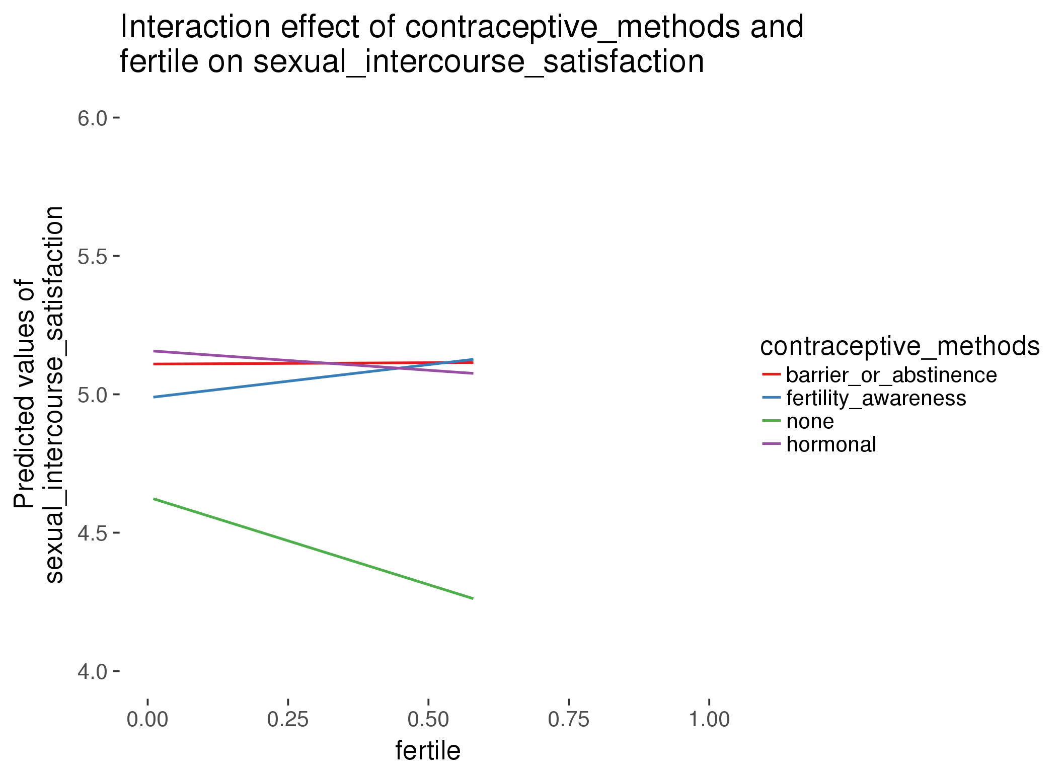
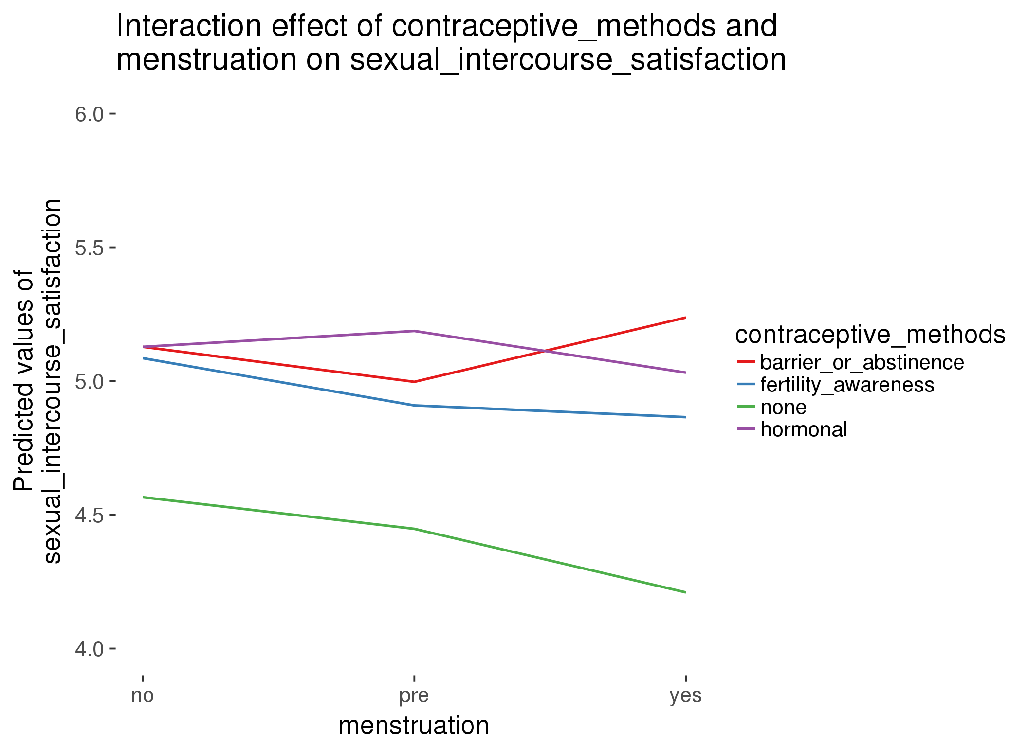
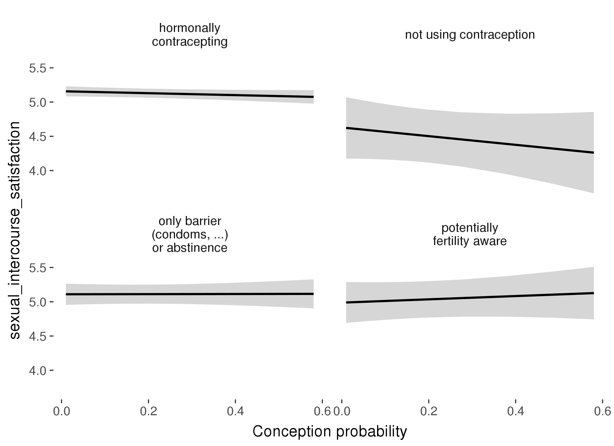
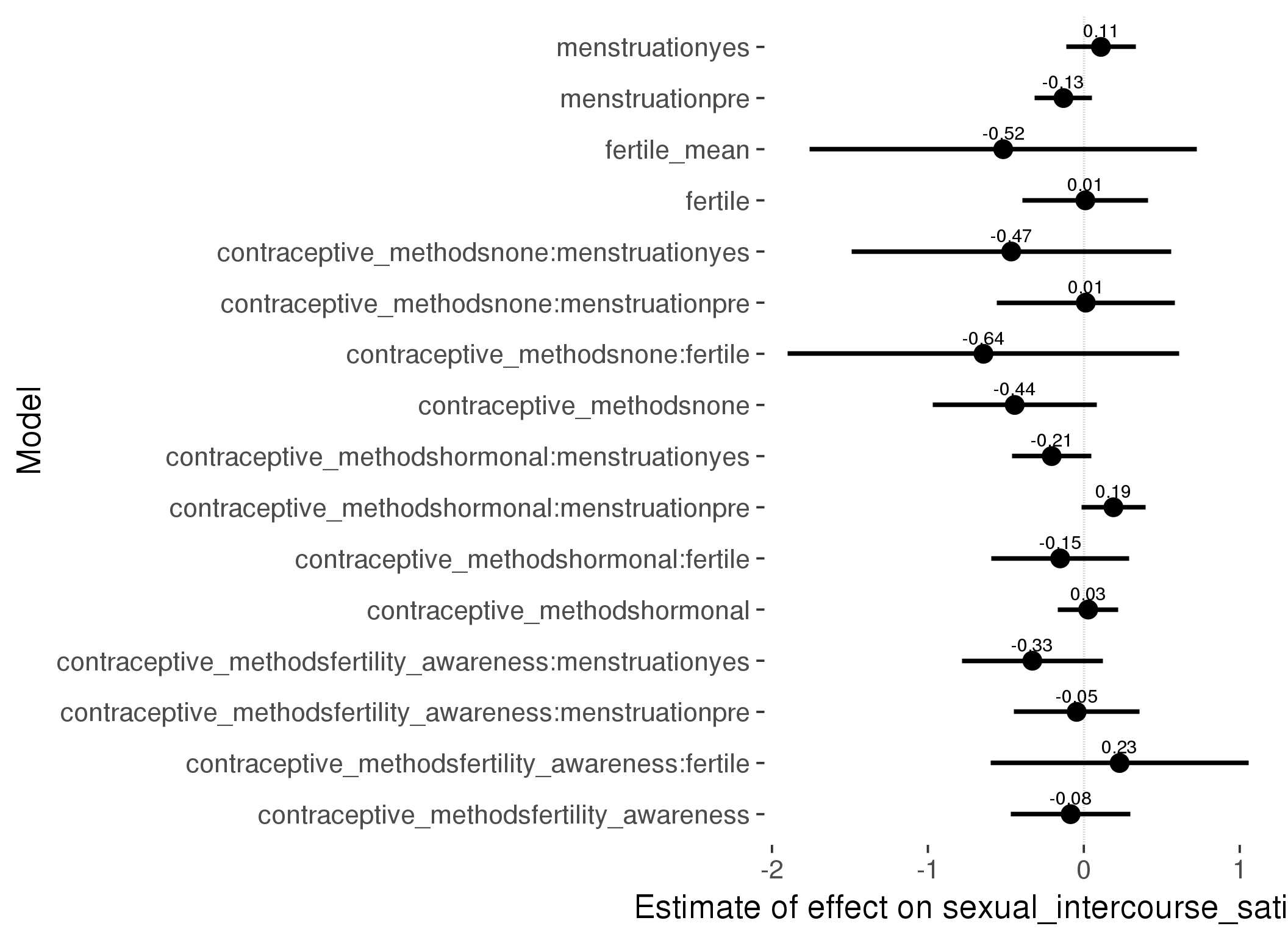
Linear mixed model fit by REML ['lmerMod']
Formula: sexual_intercourse_satisfaction ~ fertile_mean + (1 | person) +
contraceptive_methods + fertile + menstruation + fertile:contraceptive_methods +
menstruation:contraceptive_methods
Data: diary
Subset: !is.na(included_lax) & contraceptive_method != "other"
REML criterion at convergence: 9254
Scaled residuals:
Min 1Q Median 3Q Max
-5.239 -0.550 0.154 0.659 2.650
Random effects:
Groups Name Variance Std.Dev.
person (Intercept) 0.297 0.545
Residual 0.611 0.782
Number of obs: 3648, groups: person, 470
Fixed effects:
Estimate Std. Error t value
(Intercept) 5.21738 0.13413 38.9
fertile_mean -0.51699 0.63327 -0.8
contraceptive_methodsfertility_awareness -0.08470 0.19473 -0.4
contraceptive_methodsnone -0.44323 0.26809 -1.7
contraceptive_methodshormonal 0.02822 0.09864 0.3
fertile 0.00995 0.20524 0.0
menstruationpre -0.13066 0.09382 -1.4
menstruationyes 0.10969 0.11344 1.0
contraceptive_methodsfertility_awareness:fertile 0.22959 0.42250 0.5
contraceptive_methodsnone:fertile -0.64355 0.64121 -1.0
contraceptive_methodshormonal:fertile -0.15156 0.22549 -0.7
contraceptive_methodsfertility_awareness:menstruationpre -0.04603 0.20604 -0.2
contraceptive_methodsnone:menstruationpre 0.01257 0.29155 0.0
contraceptive_methodshormonal:menstruationpre 0.18988 0.10458 1.8
contraceptive_methodsfertility_awareness:menstruationyes -0.33015 0.23064 -1.4
contraceptive_methodsnone:menstruationyes -0.46542 0.52285 -0.9
contraceptive_methodshormonal:menstruationyes -0.20615 0.13008 -1.6
refitting model(s) with ML (instead of REML)
| Df | AIC | BIC | logLik | deviance | Chisq | Chi Df | Pr(>Chisq) | |
|---|---|---|---|---|---|---|---|---|
| add_main | 13 | 9253 | 9334 | -4614 | 9227 | NA | NA | NA |
| by_method | 19 | 9259 | 9377 | -4611 | 9221 | 6.118 | 6 | 0.4101 |
M_m2: Moderation by participant age
model %>%
test_moderator("age_group", diary, xlevels = 5)refitting model(s) with ML (instead of REML)
| Df | AIC | BIC | logLik | deviance | Chisq | Chi Df | Pr(>Chisq) | |
|---|---|---|---|---|---|---|---|---|
| with_main | 19 | 14993 | 15120 | -7478 | 14955 | NA | NA | NA |
| with_mod | 27 | 15005 | 15185 | -7476 | 14951 | 4.43 | 8 | 0.8163 |
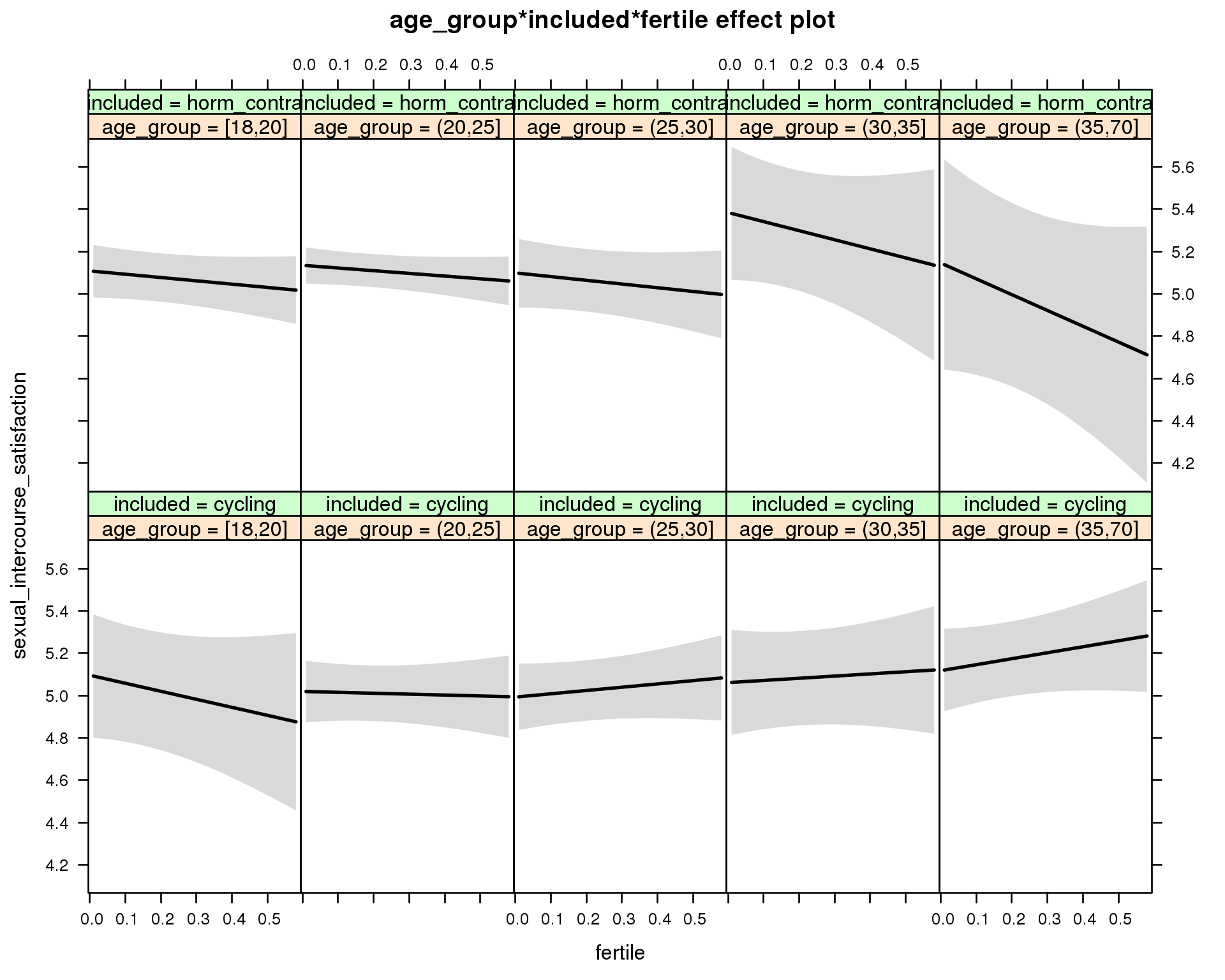
Linear mixed model fit by REML ['lmerMod']
Formula: sexual_intercourse_satisfaction ~ menstruation + fertile_mean +
(1 | person) + age_group + included + fertile + menstruation:included +
age_group:included + age_group:fertile + included:fertile + age_group:included:fertile
Data: diary
REML criterion at convergence: 15008
Scaled residuals:
Min 1Q Median 3Q Max
-5.069 -0.530 0.165 0.646 2.821
Random effects:
Groups Name Variance Std.Dev.
person (Intercept) 0.321 0.566
Residual 0.652 0.807
Number of obs: 5747, groups: person, 859
Fixed effects:
Estimate Std. Error t value
(Intercept) 5.10899 0.15891 32.2
menstruationpre -0.01968 0.05734 -0.3
menstruationyes -0.05761 0.06298 -0.9
fertile_mean -0.02124 0.35060 -0.1
age_group(20,25] -0.07647 0.16641 -0.5
age_group(25,30] -0.10313 0.16931 -0.6
age_group(30,35] -0.03486 0.19598 -0.2
age_group(35,70] 0.02180 0.17950 0.1
includedhorm_contra 0.00418 0.16550 0.0
fertile -0.37924 0.37047 -1.0
menstruationpre:includedhorm_contra 0.04769 0.07082 0.7
menstruationyes:includedhorm_contra -0.00591 0.08296 -0.1
age_group(20,25]:includedhorm_contra 0.10297 0.18345 0.6
age_group(25,30]:includedhorm_contra 0.09386 0.19909 0.5
age_group(30,35]:includedhorm_contra 0.31077 0.26220 1.2
age_group(35,70]:includedhorm_contra 0.01536 0.31926 0.0
age_group(20,25]:fertile 0.33662 0.40434 0.8
age_group(25,30]:fertile 0.53488 0.40455 1.3
age_group(30,35]:fertile 0.48245 0.45587 1.1
age_group(35,70]:fertile 0.66149 0.43817 1.5
includedhorm_contra:fertile 0.22305 0.39721 0.6
age_group(20,25]:includedhorm_contra:fertile -0.30770 0.43849 -0.7
age_group(25,30]:includedhorm_contra:fertile -0.55413 0.46583 -1.2
age_group(30,35]:includedhorm_contra:fertile -0.75531 0.64656 -1.2
age_group(35,70]:includedhorm_contra:fertile -1.25232 0.75326 -1.7
M_m3: Moderation by weekend
model %>%
test_moderator("weekend", diary, xlevels = 2) refitting model(s) with ML (instead of REML)
| Df | AIC | BIC | logLik | deviance | Chisq | Chi Df | Pr(>Chisq) | |
|---|---|---|---|---|---|---|---|---|
| with_main | 13 | 14986 | 15072 | -7480 | 14960 | NA | NA | NA |
| with_mod | 15 | 14989 | 15089 | -7479 | 14959 | 0.9685 | 2 | 0.6161 |
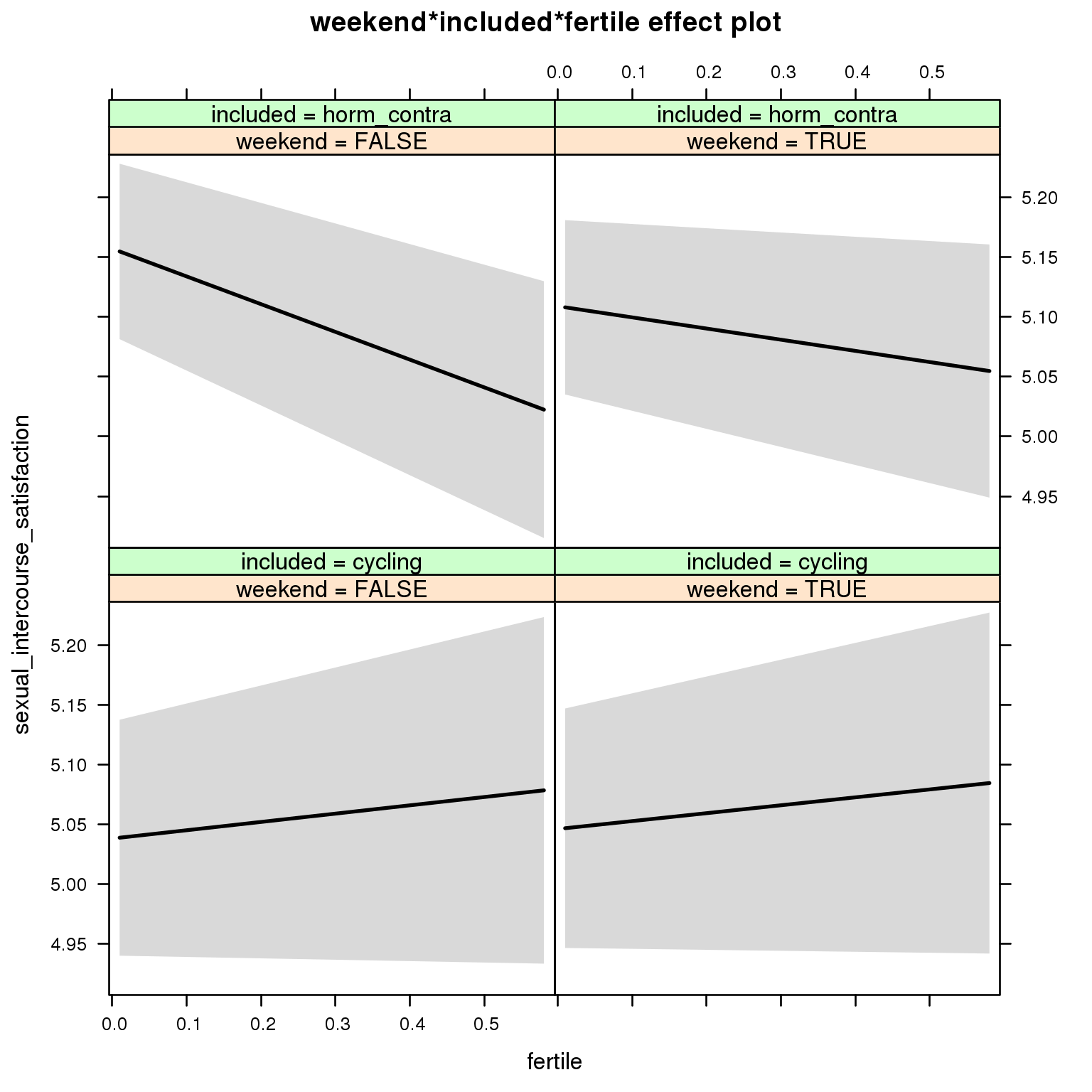
Linear mixed model fit by REML ['lmerMod']
Formula: sexual_intercourse_satisfaction ~ menstruation + fertile_mean +
(1 | person) + weekend + included + fertile + menstruation:included +
weekend:included + weekend:fertile + included:fertile + weekend:included:fertile
Data: diary
REML criterion at convergence: 15005
Scaled residuals:
Min 1Q Median 3Q Max
-5.120 -0.535 0.157 0.648 2.810
Random effects:
Groups Name Variance Std.Dev.
person (Intercept) 0.320 0.565
Residual 0.651 0.807
Number of obs: 5747, groups: person, 859
Fixed effects:
Estimate Std. Error t value
(Intercept) 5.05163 0.07951 63.5
menstruationpre -0.01851 0.05733 -0.3
menstruationyes -0.05842 0.06292 -0.9
fertile_mean -0.02493 0.34842 -0.1
weekendTRUE 0.00797 0.05214 0.2
includedhorm_contra 0.11087 0.06887 1.6
fertile 0.06945 0.15049 0.5
menstruationpre:includedhorm_contra 0.04598 0.07080 0.6
menstruationyes:includedhorm_contra -0.00431 0.08286 -0.1
weekendTRUE:includedhorm_contra -0.05605 0.06468 -0.9
weekendTRUE:fertile -0.00323 0.19315 0.0
includedhorm_contra:fertile -0.30139 0.18580 -1.6
weekendTRUE:includedhorm_contra:fertile 0.14177 0.23915 0.6
M_m4: Moderation by weekday
model %>%
test_moderator("weekday", diary, xlevels = 7)refitting model(s) with ML (instead of REML)
| Df | AIC | BIC | logLik | deviance | Chisq | Chi Df | Pr(>Chisq) | |
|---|---|---|---|---|---|---|---|---|
| with_main | 23 | 14982 | 15135 | -7468 | 14936 | NA | NA | NA |
| with_mod | 35 | 14995 | 15228 | -7463 | 14925 | 10.99 | 12 | 0.5301 |
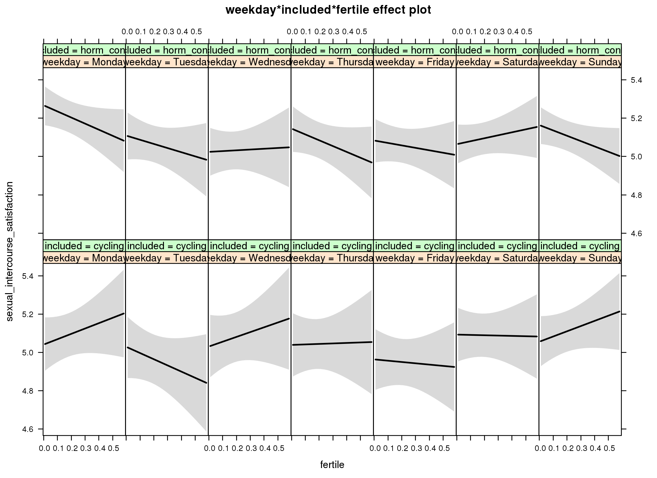
Linear mixed model fit by REML ['lmerMod']
Formula: sexual_intercourse_satisfaction ~ menstruation + fertile_mean +
(1 | person) + weekday + included + fertile + menstruation:included +
weekday:included + weekday:fertile + included:fertile + weekday:included:fertile
Data: diary
REML criterion at convergence: 15018
Scaled residuals:
Min 1Q Median 3Q Max
-5.275 -0.531 0.153 0.645 2.802
Random effects:
Groups Name Variance Std.Dev.
person (Intercept) 0.317 0.563
Residual 0.650 0.806
Number of obs: 5747, groups: person, 859
Fixed effects:
Estimate Std. Error t value
(Intercept) 5.056737 0.094334 53.6
menstruationpre -0.015387 0.057380 -0.3
menstruationyes -0.055690 0.062912 -0.9
fertile_mean -0.041111 0.348005 -0.1
weekdayTuesday -0.011875 0.097569 -0.1
weekdayWednesday -0.010121 0.098971 -0.1
weekdayThursday -0.001797 0.100787 0.0
weekdayFriday -0.077344 0.096954 -0.8
weekdaySaturday 0.052033 0.089634 0.6
weekdaySunday 0.014982 0.085147 0.2
includedhorm_contra 0.218440 0.093298 2.3
fertile 0.279274 0.250215 1.1
menstruationpre:includedhorm_contra 0.040518 0.070859 0.6
menstruationyes:includedhorm_contra 0.000669 0.082903 0.0
weekdayTuesday:includedhorm_contra -0.146252 0.122127 -1.2
weekdayWednesday:includedhorm_contra -0.232791 0.123724 -1.9
weekdayThursday:includedhorm_contra -0.119647 0.123716 -1.0
weekdayFriday:includedhorm_contra -0.106206 0.119064 -0.9
weekdaySaturday:includedhorm_contra -0.254815 0.110312 -2.3
weekdaySunday:includedhorm_contra -0.118156 0.105341 -1.1
weekdayTuesday:fertile -0.603060 0.363902 -1.7
weekdayWednesday:fertile -0.028403 0.377176 -0.1
weekdayThursday:fertile -0.253515 0.385799 -0.7
weekdayFriday:fertile -0.347338 0.355634 -1.0
weekdaySaturday:fertile -0.296297 0.336240 -0.9
weekdaySunday:fertile -0.007592 0.320762 0.0
includedhorm_contra:fertile -0.597202 0.306451 -1.9
weekdayTuesday:includedhorm_contra:fertile 0.704113 0.455862 1.5
weekdayWednesday:includedhorm_contra:fertile 0.387140 0.472235 0.8
weekdayThursday:includedhorm_contra:fertile 0.266997 0.469467 0.6
weekdayFriday:includedhorm_contra:fertile 0.537251 0.438952 1.2
weekdaySaturday:includedhorm_contra:fertile 0.769213 0.413845 1.9
weekdaySunday:includedhorm_contra:fertile 0.047356 0.394943 0.1
M_m5: Moderation by exclusion threshold
model %>%
test_moderator("included_levels", diary, xlevels = 4)refitting model(s) with ML (instead of REML)
| Df | AIC | BIC | logLik | deviance | Chisq | Chi Df | Pr(>Chisq) | |
|---|---|---|---|---|---|---|---|---|
| with_main | 17 | 14990 | 15103 | -7478 | 14956 | NA | NA | NA |
| with_mod | 23 | 14996 | 15149 | -7475 | 14950 | 5.53 | 6 | 0.4779 |
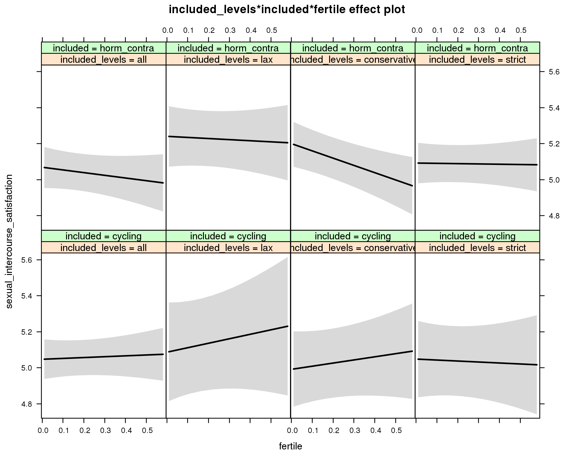
Linear mixed model fit by REML ['lmerMod']
Formula: sexual_intercourse_satisfaction ~ menstruation + fertile_mean +
(1 | person) + included_levels + included + fertile + menstruation:included +
included_levels:included + included_levels:fertile + included:fertile +
included_levels:included:fertile
Data: diary
REML criterion at convergence: 15007
Scaled residuals:
Min 1Q Median 3Q Max
-5.214 -0.531 0.153 0.650 2.823
Random effects:
Groups Name Variance Std.Dev.
person (Intercept) 0.320 0.566
Residual 0.651 0.807
Number of obs: 5747, groups: person, 859
Fixed effects:
Estimate Std. Error t value
(Intercept) 5.06634 0.08401 60.3
menstruationpre -0.01720 0.05739 -0.3
menstruationyes -0.05852 0.06291 -0.9
fertile_mean -0.05758 0.35393 -0.2
included_levelslax 0.03926 0.15075 0.3
included_levelsconservative -0.05588 0.12033 -0.5
included_levelsstrict 0.00109 0.12184 0.0
includedhorm_contra 0.01386 0.08543 0.2
fertile 0.04759 0.14275 0.3
menstruationpre:includedhorm_contra 0.04344 0.07092 0.6
menstruationyes:includedhorm_contra -0.00359 0.08290 0.0
included_levelslax:includedhorm_contra 0.13265 0.18381 0.7
included_levelsconservative:includedhorm_contra 0.18708 0.14845 1.3
included_levelsstrict:includedhorm_contra 0.02226 0.14696 0.2
included_levelslax:fertile 0.20124 0.35926 0.6
included_levelsconservative:fertile 0.12619 0.26396 0.5
included_levelsstrict:fertile -0.10212 0.27738 -0.4
includedhorm_contra:fertile -0.19727 0.20728 -1.0
included_levelslax:includedhorm_contra:fertile -0.11279 0.42997 -0.3
included_levelsconservative:includedhorm_contra:fertile -0.37996 0.33197 -1.1
included_levelsstrict:includedhorm_contra:fertile 0.23538 0.33956 0.7
M_m6: Moderation by cycle length
model %>%
test_moderator("cycle_length_groups", diary, xlevels = 4)refitting model(s) with ML (instead of REML)
| Df | AIC | BIC | logLik | deviance | Chisq | Chi Df | Pr(>Chisq) | |
|---|---|---|---|---|---|---|---|---|
| with_main | 17 | 14988 | 15101 | -7477 | 14954 | NA | NA | NA |
| with_mod | 23 | 14996 | 15149 | -7475 | 14950 | 4.201 | 6 | 0.6495 |
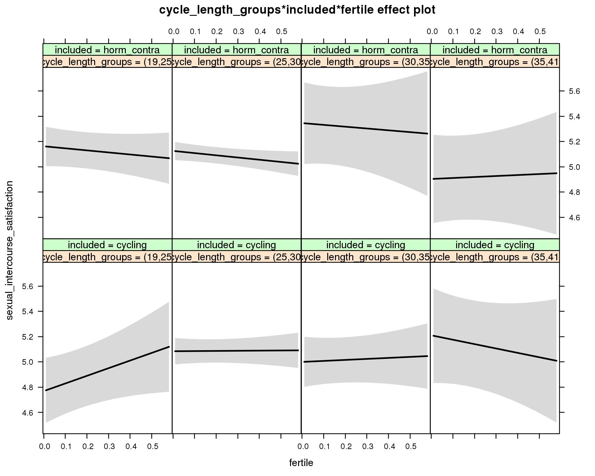
Linear mixed model fit by REML ['lmerMod']
Formula: sexual_intercourse_satisfaction ~ menstruation + fertile_mean +
(1 | person) + cycle_length_groups + included + fertile +
menstruation:included + cycle_length_groups:included + cycle_length_groups:fertile +
included:fertile + cycle_length_groups:included:fertile
Data: diary
REML criterion at convergence: 14998
Scaled residuals:
Min 1Q Median 3Q Max
-5.127 -0.534 0.159 0.655 2.880
Random effects:
Groups Name Variance Std.Dev.
person (Intercept) 0.318 0.564
Residual 0.652 0.807
Number of obs: 5747, groups: person, 859
Fixed effects:
Estimate Std. Error t value
(Intercept) 4.77888 0.14490 33.0
menstruationpre -0.02201 0.05743 -0.4
menstruationyes -0.06475 0.06318 -1.0
fertile_mean 0.00507 0.35227 0.0
cycle_length_groups(25,30] 0.31559 0.14218 2.2
cycle_length_groups(30,35] 0.23088 0.16646 1.4
cycle_length_groups(35,41] 0.44141 0.23313 1.9
includedhorm_contra 0.38488 0.15704 2.5
fertile 0.60457 0.32820 1.8
menstruationpre:includedhorm_contra 0.04585 0.07090 0.6
menstruationyes:includedhorm_contra 0.00164 0.08313 0.0
cycle_length_groups(25,30]:includedhorm_contra -0.35206 0.16714 -2.1
cycle_length_groups(30,35]:includedhorm_contra -0.04722 0.24854 -0.2
cycle_length_groups(35,41]:includedhorm_contra -0.70041 0.30464 -2.3
cycle_length_groups(25,30]:fertile -0.59270 0.34777 -1.7
cycle_length_groups(30,35]:fertile -0.52498 0.40219 -1.3
cycle_length_groups(35,41]:fertile -0.95145 0.54791 -1.7
includedhorm_contra:fertile -0.76748 0.37524 -2.0
cycle_length_groups(25,30]:includedhorm_contra:fertile 0.58046 0.39940 1.5
cycle_length_groups(30,35]:includedhorm_contra:fertile 0.54460 0.61405 0.9
cycle_length_groups(35,41]:includedhorm_contra:fertile 1.19246 0.70323 1.7
M_m7: Moderation by certainty about menstruation parameters
model %>%
test_moderator("certainty_menstruation", diary)refitting model(s) with ML (instead of REML)
| Df | AIC | BIC | logLik | deviance | Chisq | Chi Df | Pr(>Chisq) | |
|---|---|---|---|---|---|---|---|---|
| with_main | 13 | 14985 | 15071 | -7479 | 14959 | NA | NA | NA |
| with_mod | 15 | 14978 | 15078 | -7474 | 14948 | 10.97 | 2 | 0.004157 |
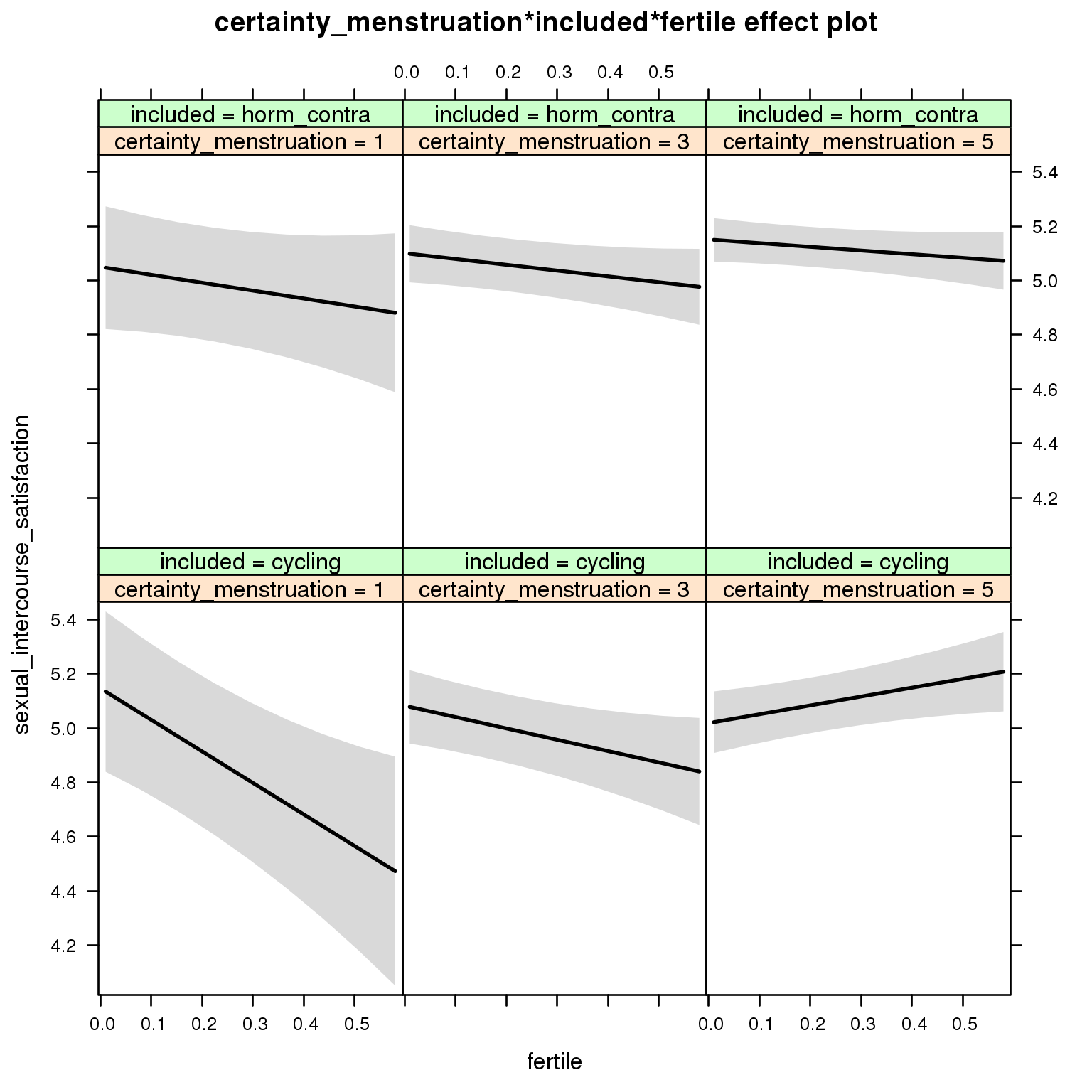
Linear mixed model fit by REML ['lmerMod']
Formula: sexual_intercourse_satisfaction ~ menstruation + fertile_mean +
(1 | person) + certainty_menstruation + included + fertile +
menstruation:included + certainty_menstruation:included +
certainty_menstruation:fertile + included:fertile + certainty_menstruation:included:fertile
Data: diary
REML criterion at convergence: 14996
Scaled residuals:
Min 1Q Median 3Q Max
-5.074 -0.529 0.157 0.652 2.810
Random effects:
Groups Name Variance Std.Dev.
person (Intercept) 0.32 0.566
Residual 0.65 0.806
Number of obs: 5747, groups: person, 859
Fixed effects:
Estimate Std. Error t value
(Intercept) 5.1923 0.2025 25.64
menstruationpre -0.0106 0.0573 -0.19
menstruationyes -0.0516 0.0629 -0.82
fertile_mean -0.0396 0.3494 -0.11
certainty_menstruation -0.0319 0.0459 -0.70
includedhorm_contra -0.1591 0.2473 -0.64
fertile -1.5323 0.5019 -3.05
menstruationpre:includedhorm_contra 0.0366 0.0708 0.52
menstruationyes:includedhorm_contra -0.0113 0.0828 -0.14
certainty_menstruation:includedhorm_contra 0.0572 0.0572 1.00
certainty_menstruation:fertile 0.3717 0.1136 3.27
includedhorm_contra:fertile 1.2020 0.6058 1.98
certainty_menstruation:includedhorm_contra:fertile -0.3327 0.1372 -2.43
M_m8: Moderation by cycle regularity
model %>%
test_moderator("cycle_regularity", diary)refitting model(s) with ML (instead of REML)
| Df | AIC | BIC | logLik | deviance | Chisq | Chi Df | Pr(>Chisq) | |
|---|---|---|---|---|---|---|---|---|
| with_main | 15 | 14976 | 15076 | -7473 | 14946 | NA | NA | NA |
| with_mod | 19 | 14983 | 15110 | -7473 | 14945 | 1.029 | 4 | 0.9054 |
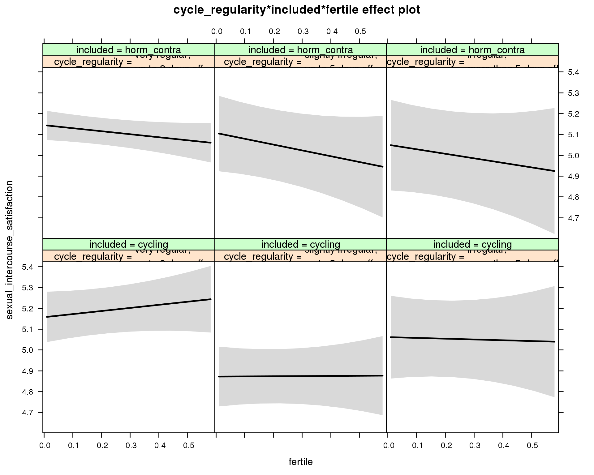
Linear mixed model fit by REML ['lmerMod']
Formula: sexual_intercourse_satisfaction ~ menstruation + fertile_mean +
(1 | person) + cycle_regularity + included + fertile + menstruation:included +
cycle_regularity:included + cycle_regularity:fertile + included:fertile +
cycle_regularity:included:fertile
Data: diary
REML criterion at convergence: 14993
Scaled residuals:
Min 1Q Median 3Q Max
-5.076 -0.533 0.154 0.653 2.761
Random effects:
Groups Name Variance Std.Dev.
person (Intercept) 0.314 0.561
Residual 0.651 0.807
Number of obs: 5747, groups: person, 859
Fixed effects:
Estimate Std. Error t value
(Intercept) 5.17122 0.08767 59.0
menstruationpre -0.01771 0.05739 -0.3
menstruationyes -0.05653 0.06293 -0.9
fertile_mean -0.02834 0.34796 -0.1
cycle_regularityslightly irregular,\nup to 5 days off -0.28510 0.09512 -3.0
cycle_regularityirregular,\nmore than 5 days off -0.09568 0.11887 -0.8
includedhorm_contra -0.02007 0.07729 -0.3
fertile 0.14861 0.15173 1.0
menstruationpre:includedhorm_contra 0.04272 0.07085 0.6
menstruationyes:includedhorm_contra -0.00673 0.08287 -0.1
cycle_regularityslightly irregular,\nup to 5 days off:includedhorm_contra 0.24762 0.13763 1.8
cycle_regularityirregular,\nmore than 5 days off:includedhorm_contra 0.00176 0.16688 0.0
cycle_regularityslightly irregular,\nup to 5 days off:fertile -0.14083 0.22026 -0.6
cycle_regularityirregular,\nmore than 5 days off:fertile -0.18625 0.28183 -0.7
includedhorm_contra:fertile -0.29384 0.17597 -1.7
cycle_regularityslightly irregular,\nup to 5 days off:includedhorm_contra:fertile 0.00687 0.31865 0.0
cycle_regularityirregular,\nmore than 5 days off:includedhorm_contra:fertile 0.11376 0.39551 0.3
M_m9: Moderation by cohabitation status
model %>%
test_moderator("cohabitation", diary)refitting model(s) with ML (instead of REML)
| Df | AIC | BIC | logLik | deviance | Chisq | Chi Df | Pr(>Chisq) | |
|---|---|---|---|---|---|---|---|---|
| with_main | 15 | 14980 | 15080 | -7475 | 14950 | NA | NA | NA |
| with_mod | 19 | 14987 | 15113 | -7474 | 14949 | 1.767 | 4 | 0.7785 |
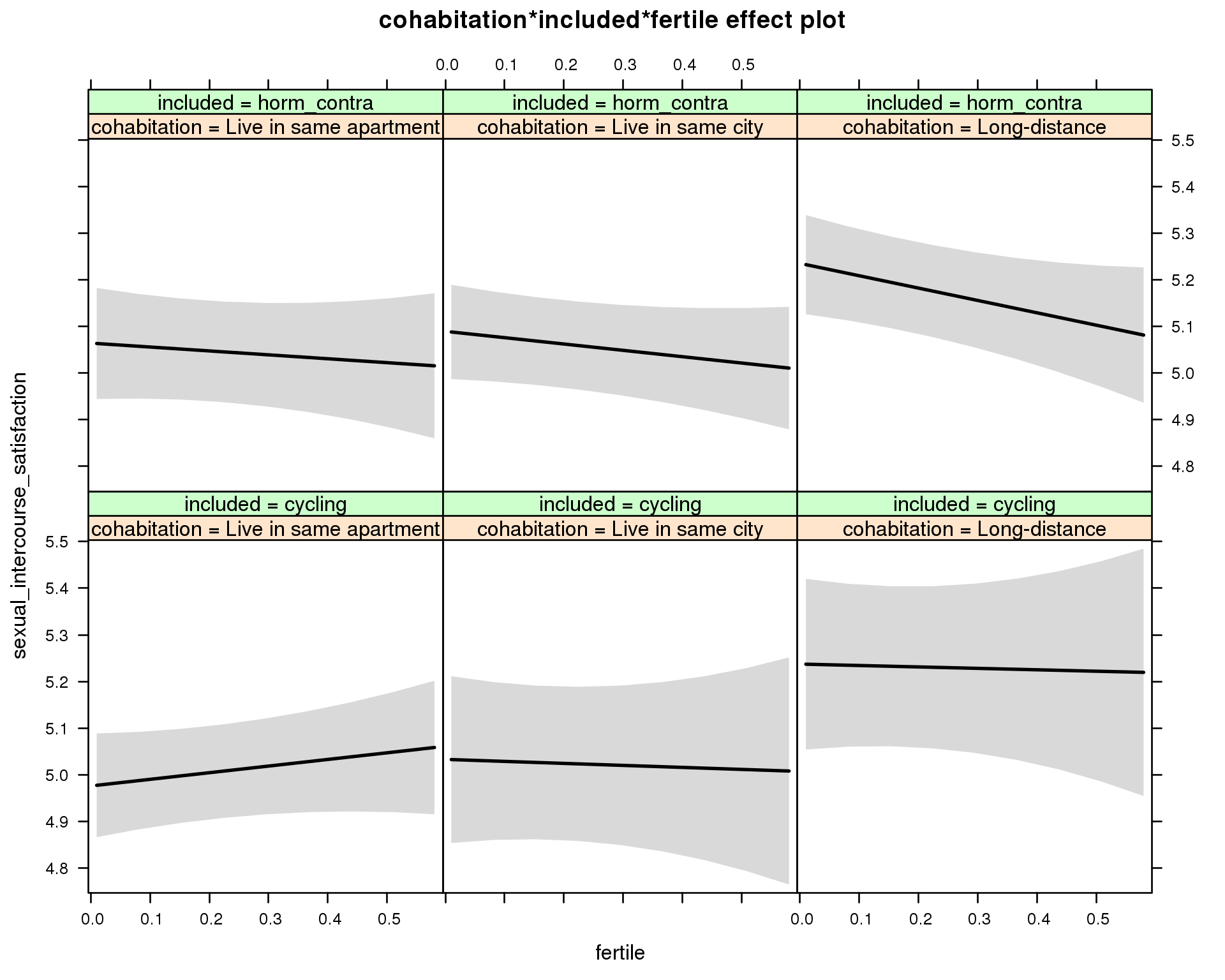
Linear mixed model fit by REML ['lmerMod']
Formula: sexual_intercourse_satisfaction ~ menstruation + fertile_mean +
(1 | person) + cohabitation + included + fertile + menstruation:included +
cohabitation:included + cohabitation:fertile + included:fertile + cohabitation:included:fertile
Data: diary
REML criterion at convergence: 15000
Scaled residuals:
Min 1Q Median 3Q Max
-5.151 -0.531 0.152 0.645 2.823
Random effects:
Groups Name Variance Std.Dev.
person (Intercept) 0.316 0.562
Residual 0.651 0.807
Number of obs: 5747, groups: person, 859
Fixed effects:
Estimate Std. Error t value
(Intercept) 4.98114 0.08547 58.3
menstruationpre -0.01967 0.05729 -0.3
menstruationyes -0.05810 0.06290 -0.9
fertile_mean 0.02455 0.34855 0.1
cohabitationLive in same city 0.05698 0.10718 0.5
cohabitationLong-distance 0.26132 0.10901 2.4
includedhorm_contra 0.08069 0.08796 0.9
fertile 0.14218 0.13701 1.0
menstruationpre:includedhorm_contra 0.04438 0.07077 0.6
menstruationyes:includedhorm_contra -0.00663 0.08285 -0.1
cohabitationLive in same city:includedhorm_contra -0.03176 0.13380 -0.2
cohabitationLong-distance:includedhorm_contra -0.09043 0.13630 -0.7
cohabitationLive in same city:fertile -0.18519 0.25380 -0.7
cohabitationLong-distance:fertile -0.17280 0.26813 -0.6
includedhorm_contra:fertile -0.22604 0.20173 -1.1
cohabitationLive in same city:includedhorm_contra:fertile 0.13314 0.31166 0.4
cohabitationLong-distance:includedhorm_contra:fertile -0.00819 0.33058 0.0
M_m10: Moderation by relationship status
model %>%
test_moderator("relationship_status_clean", diary)refitting model(s) with ML (instead of REML)
| Df | AIC | BIC | logLik | deviance | Chisq | Chi Df | Pr(>Chisq) | |
|---|---|---|---|---|---|---|---|---|
| with_main | 15 | 14986 | 15086 | -7478 | 14956 | NA | NA | NA |
| with_mod | 19 | 14994 | 15120 | -7478 | 14956 | 0.732 | 4 | 0.9473 |
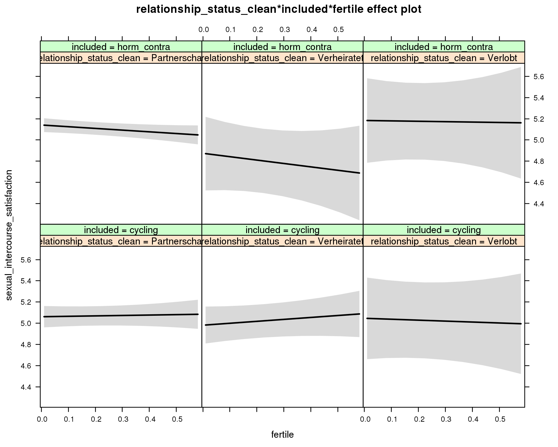
Linear mixed model fit by REML ['lmerMod']
Formula: sexual_intercourse_satisfaction ~ menstruation + fertile_mean +
(1 | person) + relationship_status_clean + included + fertile +
menstruation:included + relationship_status_clean:included +
relationship_status_clean:fertile + included:fertile + relationship_status_clean:included:fertile
Data: diary
REML criterion at convergence: 14996
Scaled residuals:
Min 1Q Median 3Q Max
-5.053 -0.531 0.159 0.649 2.805
Random effects:
Groups Name Variance Std.Dev.
person (Intercept) 0.320 0.566
Residual 0.651 0.807
Number of obs: 5747, groups: person, 859
Fixed effects:
Estimate Std. Error t value
(Intercept) 5.07125 0.07931 63.9
menstruationpre -0.02038 0.05734 -0.4
menstruationyes -0.06017 0.06300 -1.0
fertile_mean -0.00227 0.34947 0.0
relationship_status_cleanVerheiratet -0.07996 0.10263 -0.8
relationship_status_cleanVerlobt -0.01473 0.20381 -0.1
includedhorm_contra 0.07211 0.06780 1.1
fertile 0.03945 0.13316 0.3
menstruationpre:includedhorm_contra 0.04596 0.07080 0.6
menstruationyes:includedhorm_contra -0.00442 0.08294 -0.1
relationship_status_cleanVerheiratet:includedhorm_contra -0.18692 0.20916 -0.9
relationship_status_cleanVerlobt:includedhorm_contra 0.05737 0.29143 0.2
relationship_status_cleanVerheiratet:fertile 0.14346 0.23113 0.6
relationship_status_cleanVerlobt:fertile -0.12798 0.42297 -0.3
includedhorm_contra:fertile -0.20039 0.15713 -1.3
relationship_status_cleanVerheiratet:includedhorm_contra:fertile -0.30295 0.51024 -0.6
relationship_status_cleanVerlobt:includedhorm_contra:fertile 0.25129 0.66267 0.4
Spent night with partner
model_summaries$spent_night_with_partnerModel summary
Model summary
model %>%
print_summary()Generalized linear mixed model fit by maximum likelihood (Laplace Approximation) ['glmerMod']
Family: binomial ( probit )
Formula: spent_night_with_partner ~ included * (menstruation + fertile) + fertile_mean + (1 | person)
Data: diary
AIC BIC logLik deviance df.resid
26976 27058 -13478 26956 26694
Scaled residuals:
Min 1Q Median 3Q Max
-5.348 -0.599 0.127 0.516 4.813
Random effects:
Groups Name Variance Std.Dev.
person (Intercept) 1.41 1.19
Number of obs: 26704, groups: person, 1054
Fixed effects:
Estimate Std. Error z value Pr(>|z|)
(Intercept) 0.3472 0.1077 3.22 0.0013 **
includedhorm_contra -0.2135 0.0871 -2.45 0.0143 *
menstruationpre -0.0195 0.0477 -0.41 0.6823
menstruationyes -0.0207 0.0454 -0.46 0.6477
fertile -0.2111 0.0968 -2.18 0.0292 *
fertile_mean 0.4146 0.4967 0.83 0.4039
includedhorm_contra:menstruationpre -0.0683 0.0596 -1.15 0.2516
includedhorm_contra:menstruationyes -0.0960 0.0578 -1.66 0.0964 .
includedhorm_contra:fertile -0.0177 0.1195 -0.15 0.8822
---
Signif. codes: 0 '***' 0.001 '**' 0.01 '*' 0.05 '.' 0.1 ' ' 1
Correlation of Fixed Effects:
(Intr) incld_ mnstrtnp mnstrtny fertil frtl_m inclddhrm_cntr:mnstrtnp
inclddhrm_c -0.471
menstrutnpr -0.171 0.219
menstrutnys -0.165 0.210 0.393
fertile -0.164 0.272 0.464 0.384
fertile_men -0.775 -0.030 -0.008 -0.006 -0.070
inclddhrm_cntr:mnstrtnp 0.144 -0.269 -0.800 -0.315 -0.371 -0.002
inclddhrm_cntr:mnstrtny 0.135 -0.253 -0.309 -0.786 -0.301 -0.002 0.381
inclddhrm_cntr:f 0.164 -0.335 -0.376 -0.311 -0.807 0.017 0.465
inclddhrm_cntr:mnstrtny
inclddhrm_c
menstrutnpr
menstrutnys
fertile
fertile_men
inclddhrm_cntr:mnstrtnp
inclddhrm_cntr:mnstrtny
inclddhrm_cntr:f 0.380
Effect size standardised by residual variance (\(\frac{b}{ SD_{residual} }\)): -0.21 [-0.40;-0.02].
Marginal effect plots
model %>%
plot_all_effects()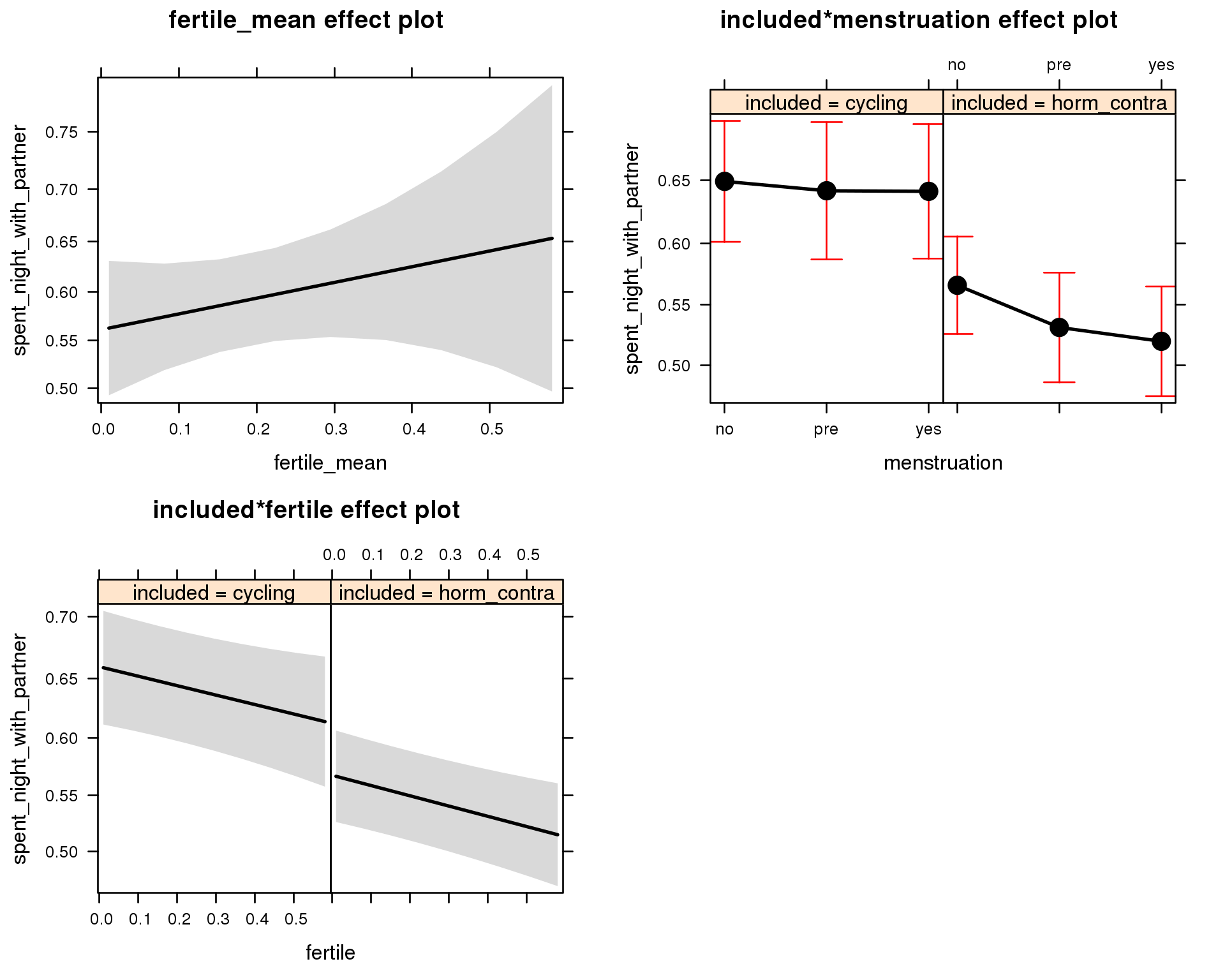
Outcome distribution
model %>%
plot_outcome(diary) + xlab(outcome_label)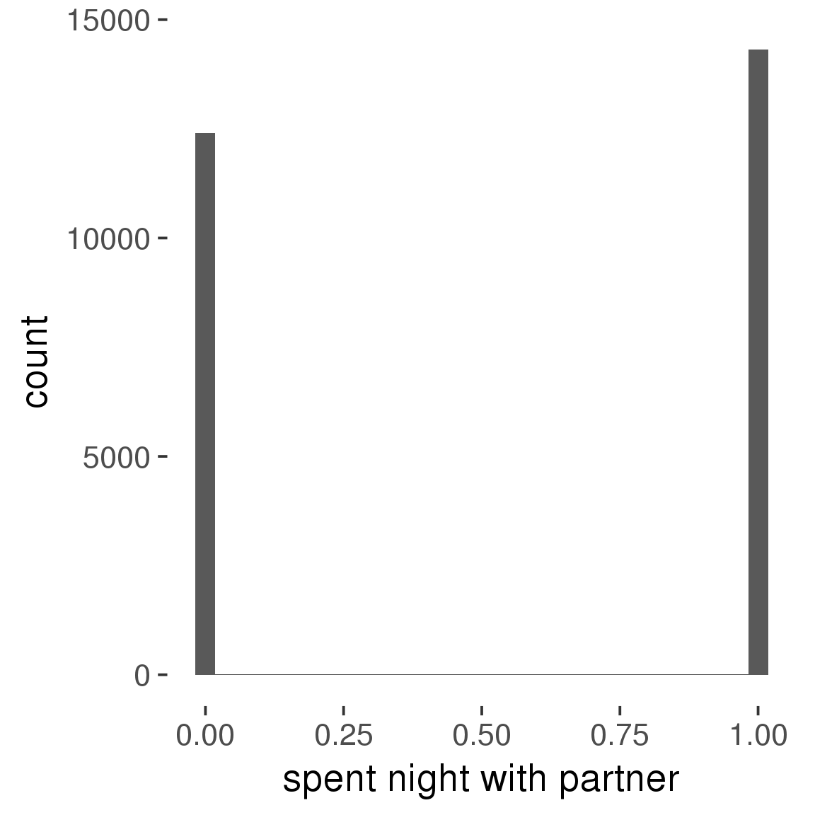
Diagnostics
model %>%
print_diagnostics()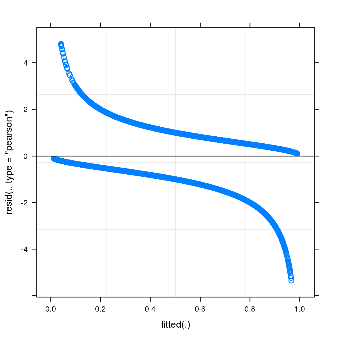
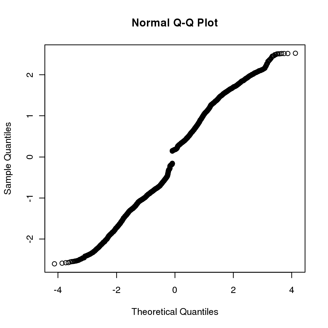
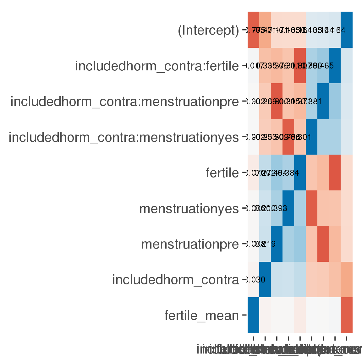
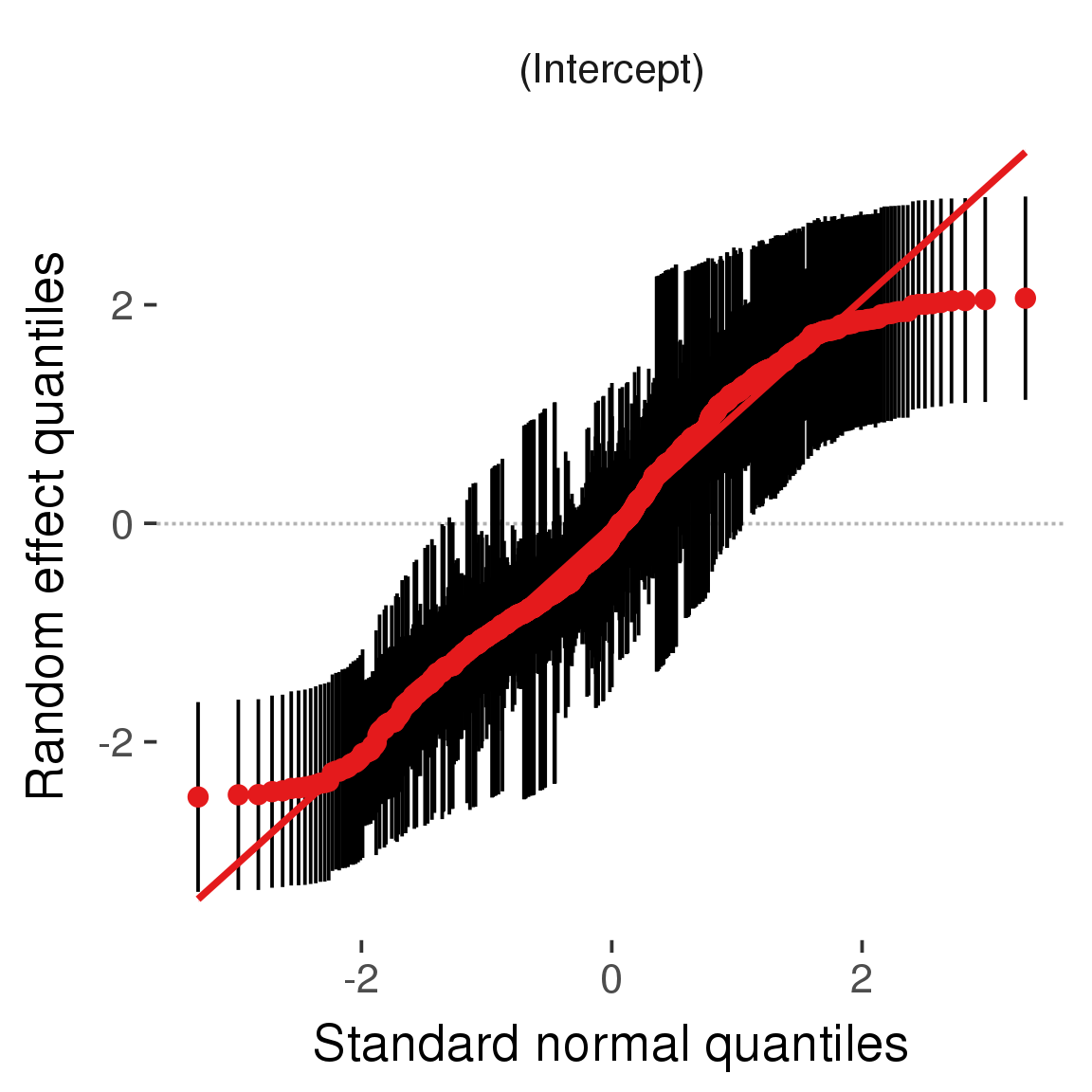
Curves
Here, we continuously plot the outcome over the course of the cycle. Because cycle lengths vary, we subset the data to cycles in a certain range. If the red curve traces the pink curve, our predictor accurately maps the relationship between fertile window probability and the outcome.
Cycle lengths from 21 to 36
Backward-counted
model %>%
plot_curve(diary %>% filter(minimum_cycle_length_diary <= 36, minimum_cycle_length_diary > 20) %>% mutate(fertile=prc_stirn_b))outcome = names(model@frame)[1]
outcome_label = recode(str_replace_all(str_replace_all(str_replace_all(outcome, "_", " "), " pair", "-pair"), " 1", ""),
"desirability 1" = "self-perceived desirability",
"NARQ admiration" = "narcissistic admiration",
"NARQ rivalry" = "narcissistic rivalry",
"extra-pair" = "extra-pair desire & behaviour",
"had sexual intercourse" = "sexual intercourse")
library(ggplot2)
# form a subset and run the model without the hormonal contraception and the fertility predictors
tmp = diary %>%
filter(!is.na(fertile), !is.na(included),
RCD > -1 * minimum_cycle_length_diary, RCD > -40)
new_form = update.formula(formula(model), new = . ~ . - fertile * included)
tmp$residuals = residuals(update(model, new_form, data = tmp , na.action = na.exclude))
tmp = tmp %>%
filter(!is.na(RCD), !is.na(residuals))
rcd_min = min(tmp$RCD)
tmp$real = FALSE
tmp_before = tmp
tmp_before$RCD = tmp_before$RCD + min(tmp$RCD) - 1
tmp_after = tmp
tmp_after$RCD = tmp_after$RCD - min(tmp$RCD) + 1
tmp$real = TRUE
tmp = bind_rows(tmp_before %>% filter(RCD > rcd_min - 11), tmp, tmp_after %>% filter(RCD < 11))GAM smooth on residuals
Here, we partialled out menstruation and individual random effects, then superimposed estimated probability of being in the fertile window scaled to the range of the estimated means. To address the periodicity of the cycle, we prepended and appended ten days of the timeseries to the end and the beginning of the timeseries. We then estimated the GAM and cut off the appended subsets before plotting.
tryCatch({
trend_plot = ggplot(tmp,aes(x = RCD, y = residuals, colour = included)) +
stat_smooth(geom = 'smooth',size = 0.8, fill = "#9ECAE1", method = 'gam', formula = y ~ s(x))
}, error = function(e){cat_message(e, "danger")})
tryCatch({
trend_data = ggplot_build(trend_plot)$data[[1]]
}, error = function(e){cat_message(e, "danger")})
trend_data$RCD = round(trend_data$x)
trend_data = left_join(trend_data, tmp %>% select(real, RCD,fertile) %>% unique(), by = "RCD")
trend_data %>%
filter(real == TRUE) %>%
mutate(superimposed = ( ( (fertile - 0.01)/0.58) * (max(y)-min(y) ) ) + min(y) ) ->
trend_data
ggplot(trend_data) +
geom_ribbon(aes(x = x, ymin = ymin, ymax = ymax, fill = factor(group)), alpha = 0.2) +
geom_line(aes(x = x, y = y, colour = factor(group)), size = 0.8, stat = "identity") +
scale_x_continuous(caption_x) +
geom_line(aes(x = x, y = superimposed), color = "#a83fbf", size = 1, linetype = 'dashed') +
annotate("text",x = mean(trend_data$x), y = max(trend_data$superimposed,na.rm=T) + 0.1, label = 'superimposed fertility peak', color = "#a83fbf") +
scale_y_continuous(outcome_label) +
ggtitle("GAM smooth, residuals") +
scale_color_manual("Contraception status",values = c("2"="black","1"= "red"), labels = c("2"="hormonally\ncontracepting","1"="cycling"), guide = F) +
scale_fill_manual("Contraception status",values = c("2"="black","1"= "red"), labels = c("2"="hormonally\ncontracepting","1"="cycling"), guide = F)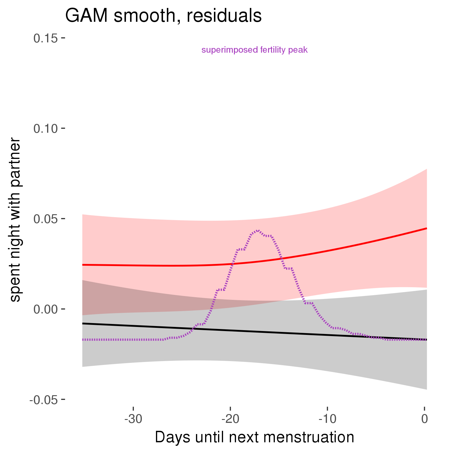
GAM smooth on raw data
As before, but without partialling anything out.
tryCatch({
trend_plot = ggplot(tmp,aes_string(x = "RCD", y = outcome, colour = "included")) +
stat_smooth(geom = 'smooth',size = 0.8, fill = "#9ECAE1", method = 'gam', formula = y ~ s(x))
}, error = function(e){cat_message(e, "danger")})
tryCatch({
trend_data = ggplot_build(trend_plot)$data[[1]]
}, error = function(e){cat_message(e, "danger")})
trend_data$RCD = round(trend_data$x)
trend_data = left_join(trend_data, tmp %>% select(real, RCD,fertile) %>% unique(), by = "RCD")
trend_data %>%
filter(real == TRUE) %>%
mutate(superimposed = ( ( (fertile - 0.01)/0.58) * (max(y)-min(y) ) ) + min(y) ) ->
trend_data
plot1b = ggplot(trend_data) +
geom_ribbon(aes(x = x, ymin = ymin, ymax = ymax, fill = factor(group)), alpha = 0.2) +
geom_line(aes(x = x, y = y, colour = factor(group)), size = 0.8, stat = "identity") +
scale_x_continuous(caption_x) +
geom_line(aes(x = x, y = superimposed), color = "#a83fbf", size = 1, linetype = 'dashed') +
annotate("text",x = mean(trend_data$x), y = max(trend_data$superimposed,na.rm=T) + 0.1, label = 'superimposed fertility peak', color = "#a83fbf") +
scale_y_continuous(outcome_label) +
ggtitle("GAM smooth, raw data") +
scale_color_manual("Contraception status",values = c("2"="black","1"= "red"), labels = c("2"="hormonally\ncontracepting","1"="cycling"), guide = F) +
scale_fill_manual("Contraception status",values = c("2"="black","1"= "red"), labels = c("2"="hormonally\ncontracepting","1"="cycling"), guide = F)
suppressWarnings(print(plot1b))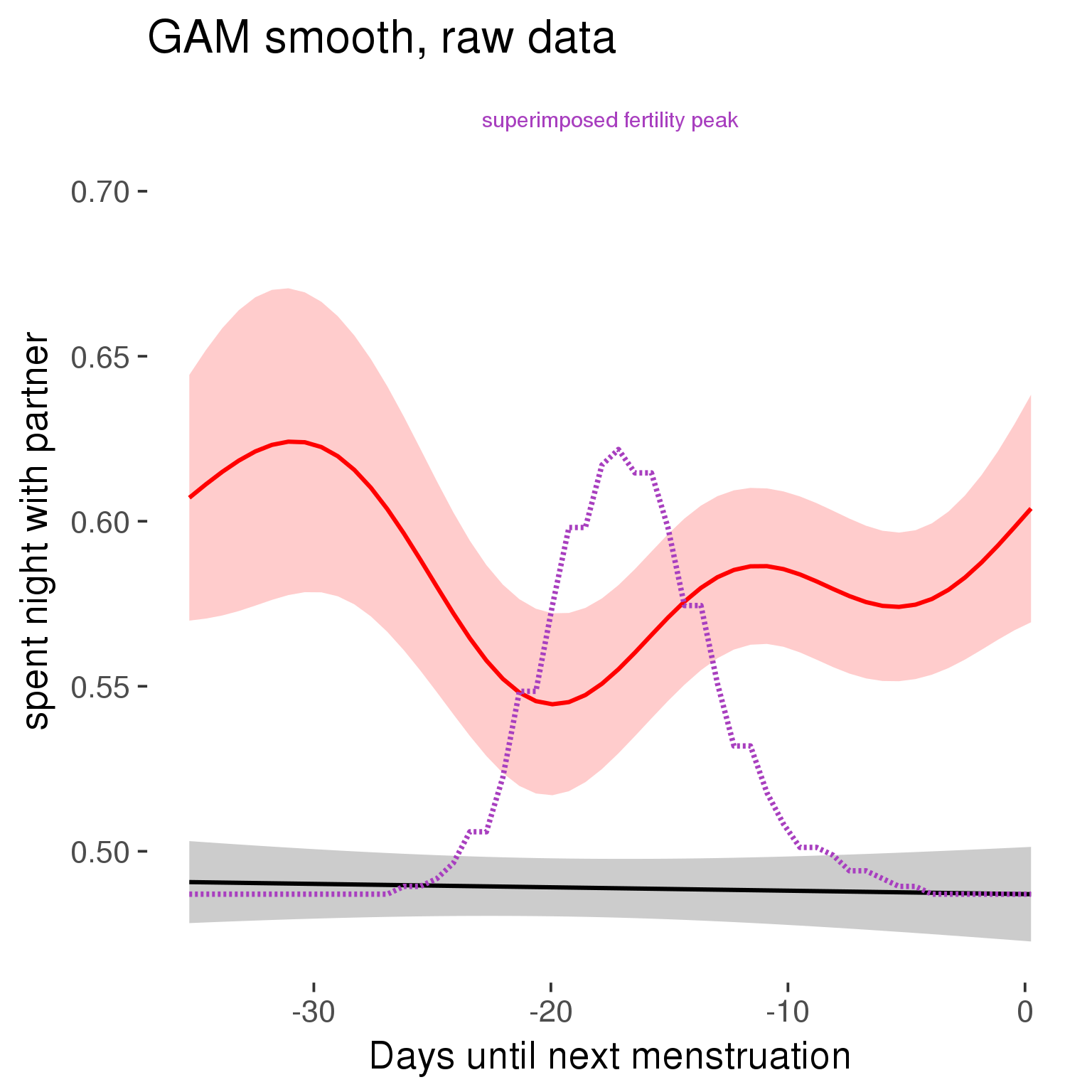
Means and standard errors over raw data
Nothing partialled out, just straight means with bootstrapped confidence intervals.
tryCatch({
trend_plot = ggplot(tmp,aes_string(x = "RCD", y = outcome, colour = "included")) +
geom_pointrange(size = 0.8, stat = 'summary', fun.data = "mean_cl_boot")
}, error = function(e){cat_message(e, "danger")})
tryCatch({
trend_data = ggplot_build(trend_plot)$data[[1]]
}, error = function(e){cat_message(e, "danger")})
trend_data$RCD = round(trend_data$x)
trend_data = left_join(trend_data, tmp %>% select(real, RCD,fertile) %>% unique(), by = "RCD")
trend_data %>%
filter(real == TRUE) %>%
mutate(superimposed = ( ( (fertile - 0.01)/0.58) * (max(y)-min(y) ) ) + min(y) ) ->
trend_data
plot3 = ggplot(trend_data) +
geom_pointrange(aes(x = x, y = y, ymin = ymin,ymax = ymax, colour = factor(group)), size = 0.8, stat = "identity", alpha = 0.6, position = position_dodge(width = .5)) +
scale_x_continuous("Days until next menstruation") +
geom_line(aes(x= x, y = superimposed), color = "#a83fbf", size = 1, linetype = 'dashed') +
annotate("text",x = mean(trend_data$x), y = max(trend_data$superimposed,na.rm=T) + 0.1, label = 'superimposed fertility peak', color = "#a83fbf") +
scale_y_continuous(outcome_label) +
ggtitle("Means with standard errors, raw data") +
scale_color_manual("Contraception status",values = c("2"="black","1"= "red"), labels = c("2"="hormonally\ncontracepting","1"="cycling"), guide = F) +
scale_fill_manual("Contraception status",values = c("2"="black","1"= "red"), labels = c("2"="hormonally\ncontracepting","1"="cycling"), guide = F)
suppressWarnings(print(plot3))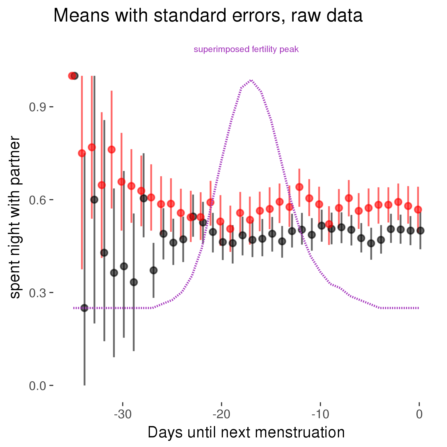
Forward-counted
model %>%
plot_curve(diary %>% filter(minimum_cycle_length_diary <= 36, minimum_cycle_length_diary > 20) %>% mutate(RCD = FCD, fertile = prc_stirn_b_forward_counted), caption_x = "Days since last menstruation")outcome = names(model@frame)[1]
outcome_label = recode(str_replace_all(str_replace_all(str_replace_all(outcome, "_", " "), " pair", "-pair"), " 1", ""),
"desirability 1" = "self-perceived desirability",
"NARQ admiration" = "narcissistic admiration",
"NARQ rivalry" = "narcissistic rivalry",
"extra-pair" = "extra-pair desire & behaviour",
"had sexual intercourse" = "sexual intercourse")
library(ggplot2)
# form a subset and run the model without the hormonal contraception and the fertility predictors
tmp = diary %>%
filter(!is.na(fertile), !is.na(included),
RCD > -1 * minimum_cycle_length_diary, RCD > -40)
new_form = update.formula(formula(model), new = . ~ . - fertile * included)
tmp$residuals = residuals(update(model, new_form, data = tmp , na.action = na.exclude))
tmp = tmp %>%
filter(!is.na(RCD), !is.na(residuals))
rcd_min = min(tmp$RCD)
tmp$real = FALSE
tmp_before = tmp
tmp_before$RCD = tmp_before$RCD + min(tmp$RCD) - 1
tmp_after = tmp
tmp_after$RCD = tmp_after$RCD - min(tmp$RCD) + 1
tmp$real = TRUE
tmp = bind_rows(tmp_before %>% filter(RCD > rcd_min - 11), tmp, tmp_after %>% filter(RCD < 11))GAM smooth on residuals
Here, we partialled out menstruation and individual random effects, then superimposed estimated probability of being in the fertile window scaled to the range of the estimated means. To address the periodicity of the cycle, we prepended and appended ten days of the timeseries to the end and the beginning of the timeseries. We then estimated the GAM and cut off the appended subsets before plotting.
tryCatch({
trend_plot = ggplot(tmp,aes(x = RCD, y = residuals, colour = included)) +
stat_smooth(geom = 'smooth',size = 0.8, fill = "#9ECAE1", method = 'gam', formula = y ~ s(x))
}, error = function(e){cat_message(e, "danger")})
tryCatch({
trend_data = ggplot_build(trend_plot)$data[[1]]
}, error = function(e){cat_message(e, "danger")})
trend_data$RCD = round(trend_data$x)
trend_data = left_join(trend_data, tmp %>% select(real, RCD,fertile) %>% unique(), by = "RCD")
trend_data %>%
filter(real == TRUE) %>%
mutate(superimposed = ( ( (fertile - 0.01)/0.58) * (max(y)-min(y) ) ) + min(y) ) ->
trend_data
ggplot(trend_data) +
geom_ribbon(aes(x = x, ymin = ymin, ymax = ymax, fill = factor(group)), alpha = 0.2) +
geom_line(aes(x = x, y = y, colour = factor(group)), size = 0.8, stat = "identity") +
scale_x_continuous(caption_x) +
geom_line(aes(x = x, y = superimposed), color = "#a83fbf", size = 1, linetype = 'dashed') +
annotate("text",x = mean(trend_data$x), y = max(trend_data$superimposed,na.rm=T) + 0.1, label = 'superimposed fertility peak', color = "#a83fbf") +
scale_y_continuous(outcome_label) +
ggtitle("GAM smooth, residuals") +
scale_color_manual("Contraception status",values = c("2"="black","1"= "red"), labels = c("2"="hormonally\ncontracepting","1"="cycling"), guide = F) +
scale_fill_manual("Contraception status",values = c("2"="black","1"= "red"), labels = c("2"="hormonally\ncontracepting","1"="cycling"), guide = F)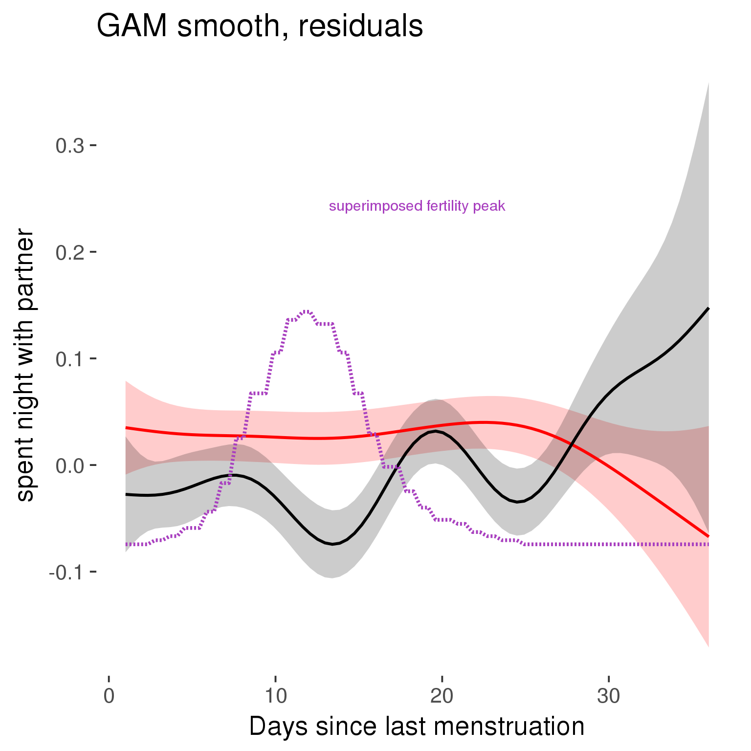
GAM smooth on raw data
As before, but without partialling anything out.
tryCatch({
trend_plot = ggplot(tmp,aes_string(x = "RCD", y = outcome, colour = "included")) +
stat_smooth(geom = 'smooth',size = 0.8, fill = "#9ECAE1", method = 'gam', formula = y ~ s(x))
}, error = function(e){cat_message(e, "danger")})
tryCatch({
trend_data = ggplot_build(trend_plot)$data[[1]]
}, error = function(e){cat_message(e, "danger")})
trend_data$RCD = round(trend_data$x)
trend_data = left_join(trend_data, tmp %>% select(real, RCD,fertile) %>% unique(), by = "RCD")
trend_data %>%
filter(real == TRUE) %>%
mutate(superimposed = ( ( (fertile - 0.01)/0.58) * (max(y)-min(y) ) ) + min(y) ) ->
trend_data
plot1b = ggplot(trend_data) +
geom_ribbon(aes(x = x, ymin = ymin, ymax = ymax, fill = factor(group)), alpha = 0.2) +
geom_line(aes(x = x, y = y, colour = factor(group)), size = 0.8, stat = "identity") +
scale_x_continuous(caption_x) +
geom_line(aes(x = x, y = superimposed), color = "#a83fbf", size = 1, linetype = 'dashed') +
annotate("text",x = mean(trend_data$x), y = max(trend_data$superimposed,na.rm=T) + 0.1, label = 'superimposed fertility peak', color = "#a83fbf") +
scale_y_continuous(outcome_label) +
ggtitle("GAM smooth, raw data") +
scale_color_manual("Contraception status",values = c("2"="black","1"= "red"), labels = c("2"="hormonally\ncontracepting","1"="cycling"), guide = F) +
scale_fill_manual("Contraception status",values = c("2"="black","1"= "red"), labels = c("2"="hormonally\ncontracepting","1"="cycling"), guide = F)
suppressWarnings(print(plot1b))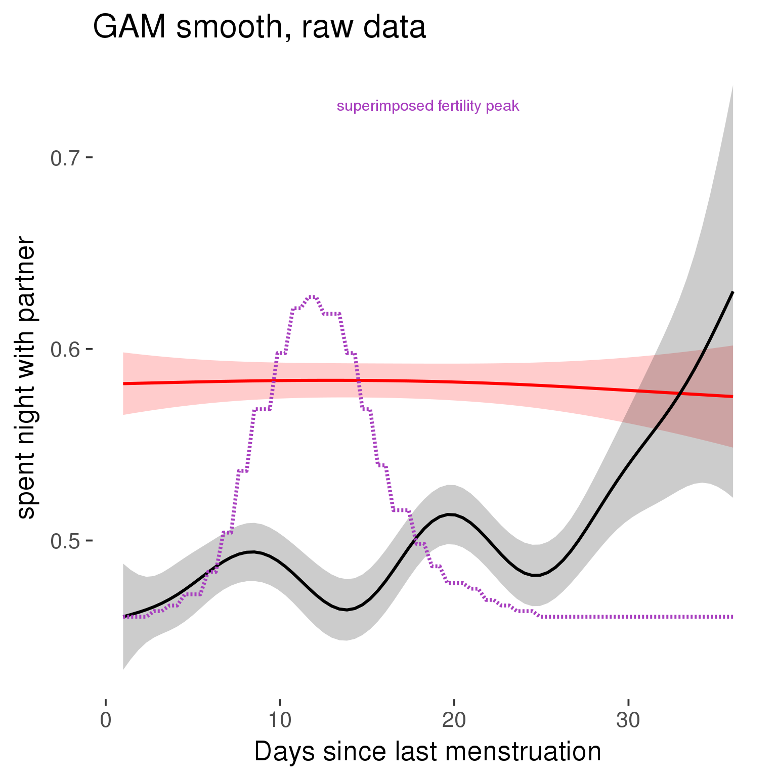
Means and standard errors over raw data
Nothing partialled out, just straight means with bootstrapped confidence intervals.
tryCatch({
trend_plot = ggplot(tmp,aes_string(x = "RCD", y = outcome, colour = "included")) +
geom_pointrange(size = 0.8, stat = 'summary', fun.data = "mean_cl_boot")
}, error = function(e){cat_message(e, "danger")})
tryCatch({
trend_data = ggplot_build(trend_plot)$data[[1]]
}, error = function(e){cat_message(e, "danger")})
trend_data$RCD = round(trend_data$x)
trend_data = left_join(trend_data, tmp %>% select(real, RCD,fertile) %>% unique(), by = "RCD")
trend_data %>%
filter(real == TRUE) %>%
mutate(superimposed = ( ( (fertile - 0.01)/0.58) * (max(y)-min(y) ) ) + min(y) ) ->
trend_data
plot3 = ggplot(trend_data) +
geom_pointrange(aes(x = x, y = y, ymin = ymin,ymax = ymax, colour = factor(group)), size = 0.8, stat = "identity", alpha = 0.6, position = position_dodge(width = .5)) +
scale_x_continuous("Days until next menstruation") +
geom_line(aes(x= x, y = superimposed), color = "#a83fbf", size = 1, linetype = 'dashed') +
annotate("text",x = mean(trend_data$x), y = max(trend_data$superimposed,na.rm=T) + 0.1, label = 'superimposed fertility peak', color = "#a83fbf") +
scale_y_continuous(outcome_label) +
ggtitle("Means with standard errors, raw data") +
scale_color_manual("Contraception status",values = c("2"="black","1"= "red"), labels = c("2"="hormonally\ncontracepting","1"="cycling"), guide = F) +
scale_fill_manual("Contraception status",values = c("2"="black","1"= "red"), labels = c("2"="hormonally\ncontracepting","1"="cycling"), guide = F)
suppressWarnings(print(plot3))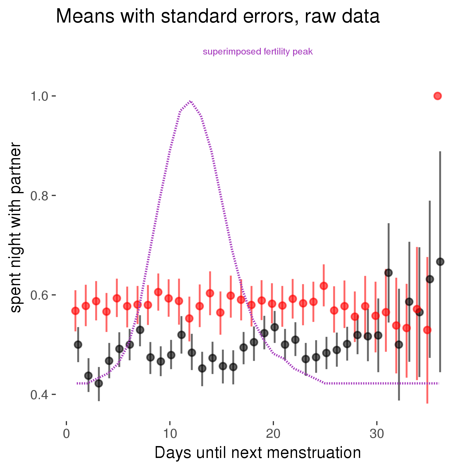
Cycle lengths from 27 to 30
Backward-counted
model %>%
plot_curve(diary %>% filter(minimum_cycle_length_diary <= 30, minimum_cycle_length_diary >= 27) %>% mutate(fertile=prc_stirn_b))outcome = names(model@frame)[1]
outcome_label = recode(str_replace_all(str_replace_all(str_replace_all(outcome, "_", " "), " pair", "-pair"), " 1", ""),
"desirability 1" = "self-perceived desirability",
"NARQ admiration" = "narcissistic admiration",
"NARQ rivalry" = "narcissistic rivalry",
"extra-pair" = "extra-pair desire & behaviour",
"had sexual intercourse" = "sexual intercourse")
library(ggplot2)
# form a subset and run the model without the hormonal contraception and the fertility predictors
tmp = diary %>%
filter(!is.na(fertile), !is.na(included),
RCD > -1 * minimum_cycle_length_diary, RCD > -40)
new_form = update.formula(formula(model), new = . ~ . - fertile * included)
tmp$residuals = residuals(update(model, new_form, data = tmp , na.action = na.exclude))
tmp = tmp %>%
filter(!is.na(RCD), !is.na(residuals))
rcd_min = min(tmp$RCD)
tmp$real = FALSE
tmp_before = tmp
tmp_before$RCD = tmp_before$RCD + min(tmp$RCD) - 1
tmp_after = tmp
tmp_after$RCD = tmp_after$RCD - min(tmp$RCD) + 1
tmp$real = TRUE
tmp = bind_rows(tmp_before %>% filter(RCD > rcd_min - 11), tmp, tmp_after %>% filter(RCD < 11))GAM smooth on residuals
Here, we partialled out menstruation and individual random effects, then superimposed estimated probability of being in the fertile window scaled to the range of the estimated means. To address the periodicity of the cycle, we prepended and appended ten days of the timeseries to the end and the beginning of the timeseries. We then estimated the GAM and cut off the appended subsets before plotting.
tryCatch({
trend_plot = ggplot(tmp,aes(x = RCD, y = residuals, colour = included)) +
stat_smooth(geom = 'smooth',size = 0.8, fill = "#9ECAE1", method = 'gam', formula = y ~ s(x))
}, error = function(e){cat_message(e, "danger")})
tryCatch({
trend_data = ggplot_build(trend_plot)$data[[1]]
}, error = function(e){cat_message(e, "danger")})
trend_data$RCD = round(trend_data$x)
trend_data = left_join(trend_data, tmp %>% select(real, RCD,fertile) %>% unique(), by = "RCD")
trend_data %>%
filter(real == TRUE) %>%
mutate(superimposed = ( ( (fertile - 0.01)/0.58) * (max(y)-min(y) ) ) + min(y) ) ->
trend_data
ggplot(trend_data) +
geom_ribbon(aes(x = x, ymin = ymin, ymax = ymax, fill = factor(group)), alpha = 0.2) +
geom_line(aes(x = x, y = y, colour = factor(group)), size = 0.8, stat = "identity") +
scale_x_continuous(caption_x) +
geom_line(aes(x = x, y = superimposed), color = "#a83fbf", size = 1, linetype = 'dashed') +
annotate("text",x = mean(trend_data$x), y = max(trend_data$superimposed,na.rm=T) + 0.1, label = 'superimposed fertility peak', color = "#a83fbf") +
scale_y_continuous(outcome_label) +
ggtitle("GAM smooth, residuals") +
scale_color_manual("Contraception status",values = c("2"="black","1"= "red"), labels = c("2"="hormonally\ncontracepting","1"="cycling"), guide = F) +
scale_fill_manual("Contraception status",values = c("2"="black","1"= "red"), labels = c("2"="hormonally\ncontracepting","1"="cycling"), guide = F)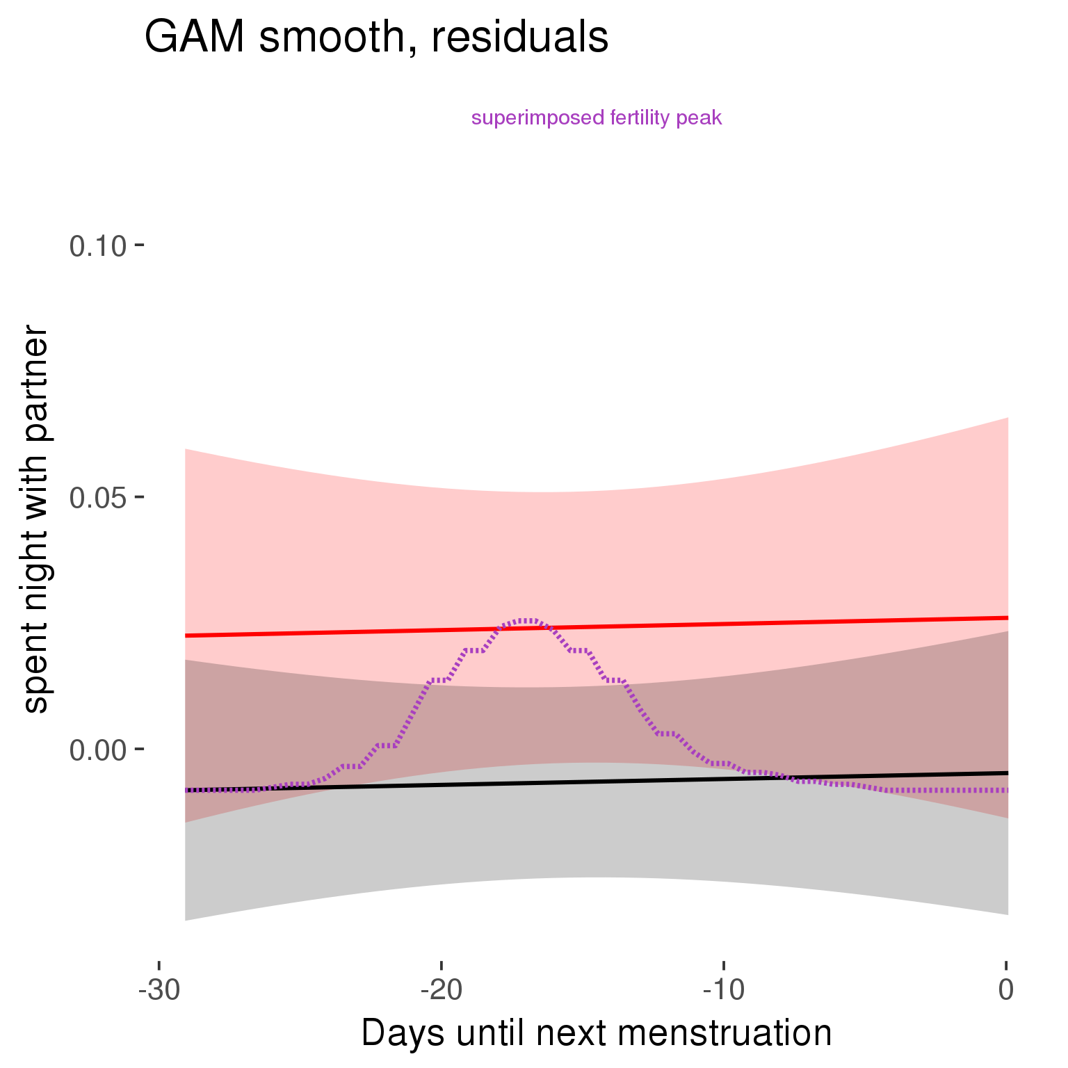
GAM smooth on raw data
As before, but without partialling anything out.
tryCatch({
trend_plot = ggplot(tmp,aes_string(x = "RCD", y = outcome, colour = "included")) +
stat_smooth(geom = 'smooth',size = 0.8, fill = "#9ECAE1", method = 'gam', formula = y ~ s(x))
}, error = function(e){cat_message(e, "danger")})
tryCatch({
trend_data = ggplot_build(trend_plot)$data[[1]]
}, error = function(e){cat_message(e, "danger")})
trend_data$RCD = round(trend_data$x)
trend_data = left_join(trend_data, tmp %>% select(real, RCD,fertile) %>% unique(), by = "RCD")
trend_data %>%
filter(real == TRUE) %>%
mutate(superimposed = ( ( (fertile - 0.01)/0.58) * (max(y)-min(y) ) ) + min(y) ) ->
trend_data
plot1b = ggplot(trend_data) +
geom_ribbon(aes(x = x, ymin = ymin, ymax = ymax, fill = factor(group)), alpha = 0.2) +
geom_line(aes(x = x, y = y, colour = factor(group)), size = 0.8, stat = "identity") +
scale_x_continuous(caption_x) +
geom_line(aes(x = x, y = superimposed), color = "#a83fbf", size = 1, linetype = 'dashed') +
annotate("text",x = mean(trend_data$x), y = max(trend_data$superimposed,na.rm=T) + 0.1, label = 'superimposed fertility peak', color = "#a83fbf") +
scale_y_continuous(outcome_label) +
ggtitle("GAM smooth, raw data") +
scale_color_manual("Contraception status",values = c("2"="black","1"= "red"), labels = c("2"="hormonally\ncontracepting","1"="cycling"), guide = F) +
scale_fill_manual("Contraception status",values = c("2"="black","1"= "red"), labels = c("2"="hormonally\ncontracepting","1"="cycling"), guide = F)
suppressWarnings(print(plot1b))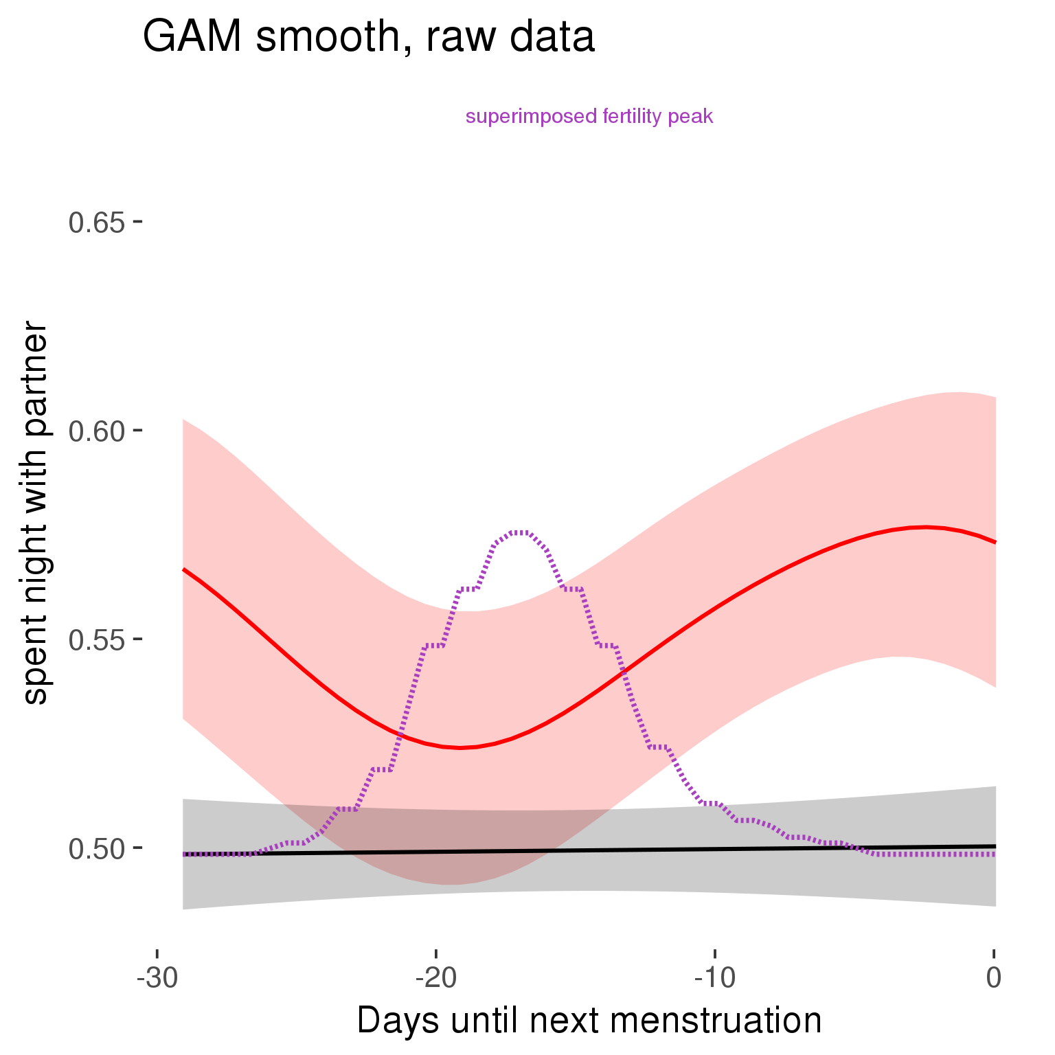
Means and standard errors over raw data
Nothing partialled out, just straight means with bootstrapped confidence intervals.
tryCatch({
trend_plot = ggplot(tmp,aes_string(x = "RCD", y = outcome, colour = "included")) +
geom_pointrange(size = 0.8, stat = 'summary', fun.data = "mean_cl_boot")
}, error = function(e){cat_message(e, "danger")})
tryCatch({
trend_data = ggplot_build(trend_plot)$data[[1]]
}, error = function(e){cat_message(e, "danger")})
trend_data$RCD = round(trend_data$x)
trend_data = left_join(trend_data, tmp %>% select(real, RCD,fertile) %>% unique(), by = "RCD")
trend_data %>%
filter(real == TRUE) %>%
mutate(superimposed = ( ( (fertile - 0.01)/0.58) * (max(y)-min(y) ) ) + min(y) ) ->
trend_data
plot3 = ggplot(trend_data) +
geom_pointrange(aes(x = x, y = y, ymin = ymin,ymax = ymax, colour = factor(group)), size = 0.8, stat = "identity", alpha = 0.6, position = position_dodge(width = .5)) +
scale_x_continuous("Days until next menstruation") +
geom_line(aes(x= x, y = superimposed), color = "#a83fbf", size = 1, linetype = 'dashed') +
annotate("text",x = mean(trend_data$x), y = max(trend_data$superimposed,na.rm=T) + 0.1, label = 'superimposed fertility peak', color = "#a83fbf") +
scale_y_continuous(outcome_label) +
ggtitle("Means with standard errors, raw data") +
scale_color_manual("Contraception status",values = c("2"="black","1"= "red"), labels = c("2"="hormonally\ncontracepting","1"="cycling"), guide = F) +
scale_fill_manual("Contraception status",values = c("2"="black","1"= "red"), labels = c("2"="hormonally\ncontracepting","1"="cycling"), guide = F)
suppressWarnings(print(plot3))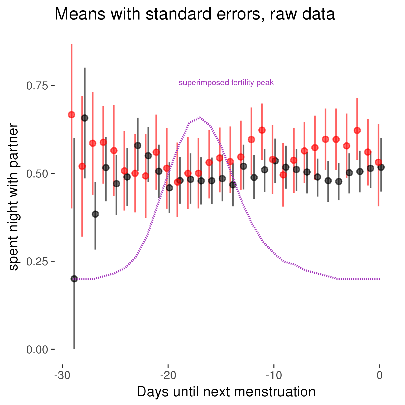
Forward-counted
model %>%
plot_curve(diary %>% filter(minimum_cycle_length_diary <= 30, minimum_cycle_length_diary >= 27) %>% mutate(RCD = FCD, fertile = prc_stirn_b_forward_counted), caption_x = "Days since last menstruation")outcome = names(model@frame)[1]
outcome_label = recode(str_replace_all(str_replace_all(str_replace_all(outcome, "_", " "), " pair", "-pair"), " 1", ""),
"desirability 1" = "self-perceived desirability",
"NARQ admiration" = "narcissistic admiration",
"NARQ rivalry" = "narcissistic rivalry",
"extra-pair" = "extra-pair desire & behaviour",
"had sexual intercourse" = "sexual intercourse")
library(ggplot2)
# form a subset and run the model without the hormonal contraception and the fertility predictors
tmp = diary %>%
filter(!is.na(fertile), !is.na(included),
RCD > -1 * minimum_cycle_length_diary, RCD > -40)
new_form = update.formula(formula(model), new = . ~ . - fertile * included)
tmp$residuals = residuals(update(model, new_form, data = tmp , na.action = na.exclude))
tmp = tmp %>%
filter(!is.na(RCD), !is.na(residuals))
rcd_min = min(tmp$RCD)
tmp$real = FALSE
tmp_before = tmp
tmp_before$RCD = tmp_before$RCD + min(tmp$RCD) - 1
tmp_after = tmp
tmp_after$RCD = tmp_after$RCD - min(tmp$RCD) + 1
tmp$real = TRUE
tmp = bind_rows(tmp_before %>% filter(RCD > rcd_min - 11), tmp, tmp_after %>% filter(RCD < 11))GAM smooth on residuals
Here, we partialled out menstruation and individual random effects, then superimposed estimated probability of being in the fertile window scaled to the range of the estimated means. To address the periodicity of the cycle, we prepended and appended ten days of the timeseries to the end and the beginning of the timeseries. We then estimated the GAM and cut off the appended subsets before plotting.
tryCatch({
trend_plot = ggplot(tmp,aes(x = RCD, y = residuals, colour = included)) +
stat_smooth(geom = 'smooth',size = 0.8, fill = "#9ECAE1", method = 'gam', formula = y ~ s(x))
}, error = function(e){cat_message(e, "danger")})
tryCatch({
trend_data = ggplot_build(trend_plot)$data[[1]]
}, error = function(e){cat_message(e, "danger")})
trend_data$RCD = round(trend_data$x)
trend_data = left_join(trend_data, tmp %>% select(real, RCD,fertile) %>% unique(), by = "RCD")
trend_data %>%
filter(real == TRUE) %>%
mutate(superimposed = ( ( (fertile - 0.01)/0.58) * (max(y)-min(y) ) ) + min(y) ) ->
trend_data
ggplot(trend_data) +
geom_ribbon(aes(x = x, ymin = ymin, ymax = ymax, fill = factor(group)), alpha = 0.2) +
geom_line(aes(x = x, y = y, colour = factor(group)), size = 0.8, stat = "identity") +
scale_x_continuous(caption_x) +
geom_line(aes(x = x, y = superimposed), color = "#a83fbf", size = 1, linetype = 'dashed') +
annotate("text",x = mean(trend_data$x), y = max(trend_data$superimposed,na.rm=T) + 0.1, label = 'superimposed fertility peak', color = "#a83fbf") +
scale_y_continuous(outcome_label) +
ggtitle("GAM smooth, residuals") +
scale_color_manual("Contraception status",values = c("2"="black","1"= "red"), labels = c("2"="hormonally\ncontracepting","1"="cycling"), guide = F) +
scale_fill_manual("Contraception status",values = c("2"="black","1"= "red"), labels = c("2"="hormonally\ncontracepting","1"="cycling"), guide = F)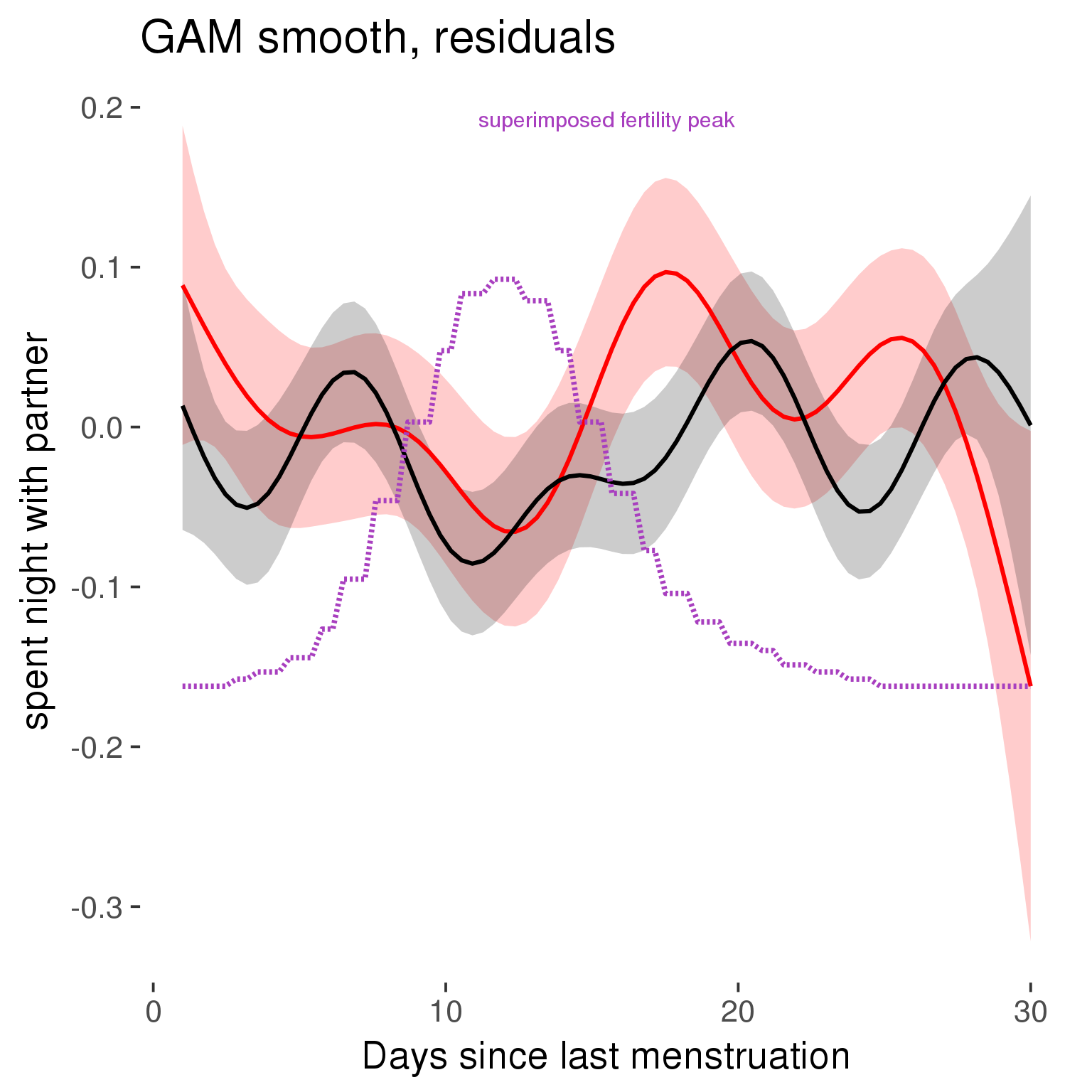
GAM smooth on raw data
As before, but without partialling anything out.
tryCatch({
trend_plot = ggplot(tmp,aes_string(x = "RCD", y = outcome, colour = "included")) +
stat_smooth(geom = 'smooth',size = 0.8, fill = "#9ECAE1", method = 'gam', formula = y ~ s(x))
}, error = function(e){cat_message(e, "danger")})
tryCatch({
trend_data = ggplot_build(trend_plot)$data[[1]]
}, error = function(e){cat_message(e, "danger")})
trend_data$RCD = round(trend_data$x)
trend_data = left_join(trend_data, tmp %>% select(real, RCD,fertile) %>% unique(), by = "RCD")
trend_data %>%
filter(real == TRUE) %>%
mutate(superimposed = ( ( (fertile - 0.01)/0.58) * (max(y)-min(y) ) ) + min(y) ) ->
trend_data
plot1b = ggplot(trend_data) +
geom_ribbon(aes(x = x, ymin = ymin, ymax = ymax, fill = factor(group)), alpha = 0.2) +
geom_line(aes(x = x, y = y, colour = factor(group)), size = 0.8, stat = "identity") +
scale_x_continuous(caption_x) +
geom_line(aes(x = x, y = superimposed), color = "#a83fbf", size = 1, linetype = 'dashed') +
annotate("text",x = mean(trend_data$x), y = max(trend_data$superimposed,na.rm=T) + 0.1, label = 'superimposed fertility peak', color = "#a83fbf") +
scale_y_continuous(outcome_label) +
ggtitle("GAM smooth, raw data") +
scale_color_manual("Contraception status",values = c("2"="black","1"= "red"), labels = c("2"="hormonally\ncontracepting","1"="cycling"), guide = F) +
scale_fill_manual("Contraception status",values = c("2"="black","1"= "red"), labels = c("2"="hormonally\ncontracepting","1"="cycling"), guide = F)
suppressWarnings(print(plot1b))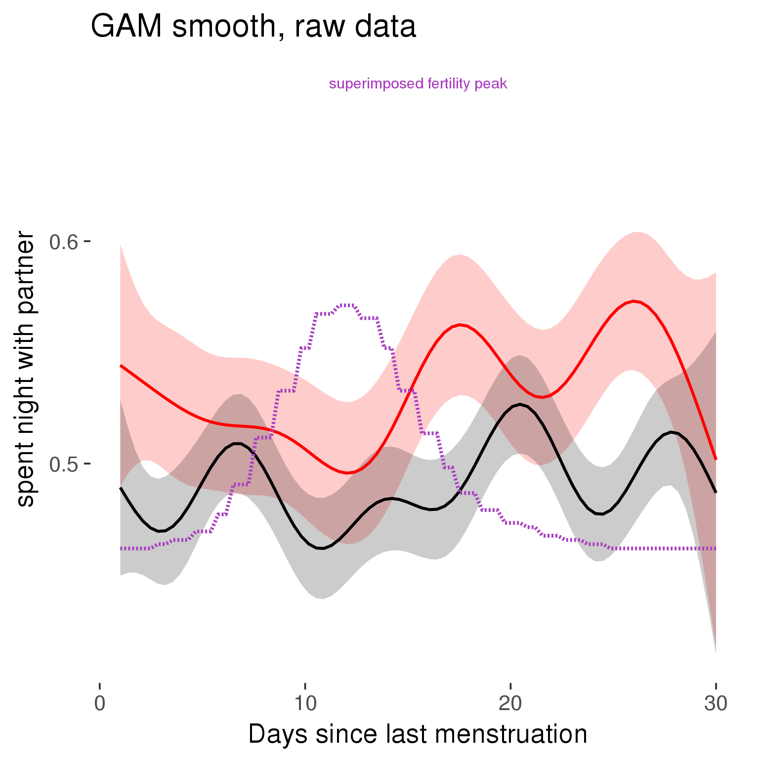
Means and standard errors over raw data
Nothing partialled out, just straight means with bootstrapped confidence intervals.
tryCatch({
trend_plot = ggplot(tmp,aes_string(x = "RCD", y = outcome, colour = "included")) +
geom_pointrange(size = 0.8, stat = 'summary', fun.data = "mean_cl_boot")
}, error = function(e){cat_message(e, "danger")})
tryCatch({
trend_data = ggplot_build(trend_plot)$data[[1]]
}, error = function(e){cat_message(e, "danger")})
trend_data$RCD = round(trend_data$x)
trend_data = left_join(trend_data, tmp %>% select(real, RCD,fertile) %>% unique(), by = "RCD")
trend_data %>%
filter(real == TRUE) %>%
mutate(superimposed = ( ( (fertile - 0.01)/0.58) * (max(y)-min(y) ) ) + min(y) ) ->
trend_data
plot3 = ggplot(trend_data) +
geom_pointrange(aes(x = x, y = y, ymin = ymin,ymax = ymax, colour = factor(group)), size = 0.8, stat = "identity", alpha = 0.6, position = position_dodge(width = .5)) +
scale_x_continuous("Days until next menstruation") +
geom_line(aes(x= x, y = superimposed), color = "#a83fbf", size = 1, linetype = 'dashed') +
annotate("text",x = mean(trend_data$x), y = max(trend_data$superimposed,na.rm=T) + 0.1, label = 'superimposed fertility peak', color = "#a83fbf") +
scale_y_continuous(outcome_label) +
ggtitle("Means with standard errors, raw data") +
scale_color_manual("Contraception status",values = c("2"="black","1"= "red"), labels = c("2"="hormonally\ncontracepting","1"="cycling"), guide = F) +
scale_fill_manual("Contraception status",values = c("2"="black","1"= "red"), labels = c("2"="hormonally\ncontracepting","1"="cycling"), guide = F)
suppressWarnings(print(plot3))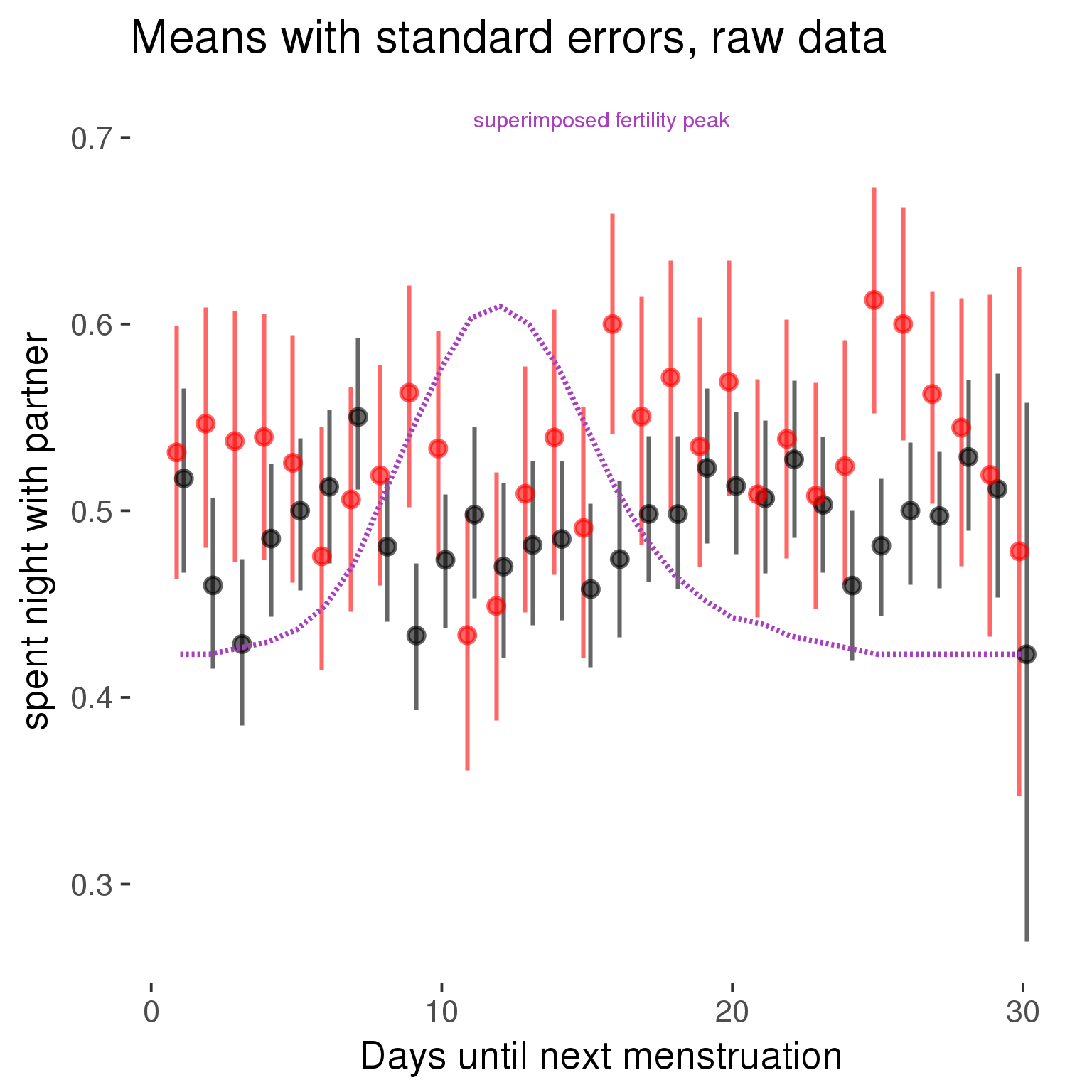
Robustness checks
M_r1: Random slopes for conception risk and menstruation
tryCatch({
# refit model with random effects for fertile and menstruation dummies
with_ind_diff = update(model, formula = . ~ . - (1| person) + (1 + fertile + menstruation | person))
# pull the random effects, format as tibble
rand = coef(with_ind_diff)$person %>%
tibble::rownames_to_column("person") %>%
mutate(person = as.numeric(person))
# pull the fixed effects
fixd = data.frame(fixef(with_ind_diff)) %>%
tibble::rownames_to_column("effect")
names(fixd) = c("effect", "pop_effect_size")
# pull apart the coefficients so that we can account for the fact that the random effect variation implicitly includes HC explaining the mean population-level effect of fertile/menstruation dummies among HC users
fixd = fixd %>%
separate(effect, c("included", "effect"), sep = ":", fill = "left") %>%
mutate(included = if_else(is.na(included), "cycling", str_replace(included, "included", "")))
fixd[2,c("included", "effect")] = c("horm_contra", "(Intercept)")
rand = rand %>%
# merge diary data on the random effects, so that we know who is a HC users and who isn't
inner_join(diary %>% select(person, included) %>% unique(), by = 'person') %>%
# gather into long format, to have the dataset by predictor
gather(effect, value, -person, -included) %>%
inner_join(fixd, by = c('effect', 'included')) %>%
# pull the fixed effects
mutate(
# only for those who are HC users, add the moderated population effect size for this effect (the random effects have the reference category mean)
value = if_else(included == "horm_contra", value + pop_effect_size, value),
effect = recode(effect, "includedhorm_contra" = "HC user",
"includedhorm_contra:fertile" = "HC user x fertile",
"includedhorm_contra:menstruationpre" = "HC user x premens.",
"includedhorm_contra:menstruationyes" = "HC user x mens.",
"menstruationyes" = "mens.",
"menstruationpre" = "premens.")) %>%
group_by(included, effect) %>%
# filter out predictors that aren't modelled as varying/random
filter(sd(value) > 0)
# plot dot plot of random effects
print(
ggplot(rand, aes(x = included, y = value, color = included, fill = included)) +
facet_wrap( ~ effect, scales = "free") +
# geom_violin(alpha = 0.4, size = 0) +
geom_dotplot(binaxis='y', dotsize = 0.1, method = "histodot") +
# geom_jitter(alpha = 0.05) +
coord_flip() +
geom_pointrange(stat = 'summary', fun.data = 'mean_sdl', color = 'darkred', size = 1.2) +
scale_color_manual("Contraception status", values = c("horm_contra"="black","cycling"= "red"), labels = c("horm_contra"="hormonally\ncontracepting","cycling"="cycling"), guide = F) +
scale_fill_manual("Contraception status", values = c("horm_contra"="black","cycling"= "red"), labels = c("horm_contra"="hormonally\ncontracepting","1"="cycling"), guide = F) +
ggtitle("M_r1: allowing participant-varying slopes", subtitle = "for the conception risk measure and the menstruation dummies") +
scale_x_discrete("Hormonal contraception", breaks = c("horm_contra", "cycling"), labels = c("yes", "no")) +
scale_y_continuous("Random effect size distribution"))
print_summary(with_ind_diff)
cat(pander(anova(model, with_ind_diff)))
}, error = function(e){
with_ind_diff = model
cat_message(e, "danger")
})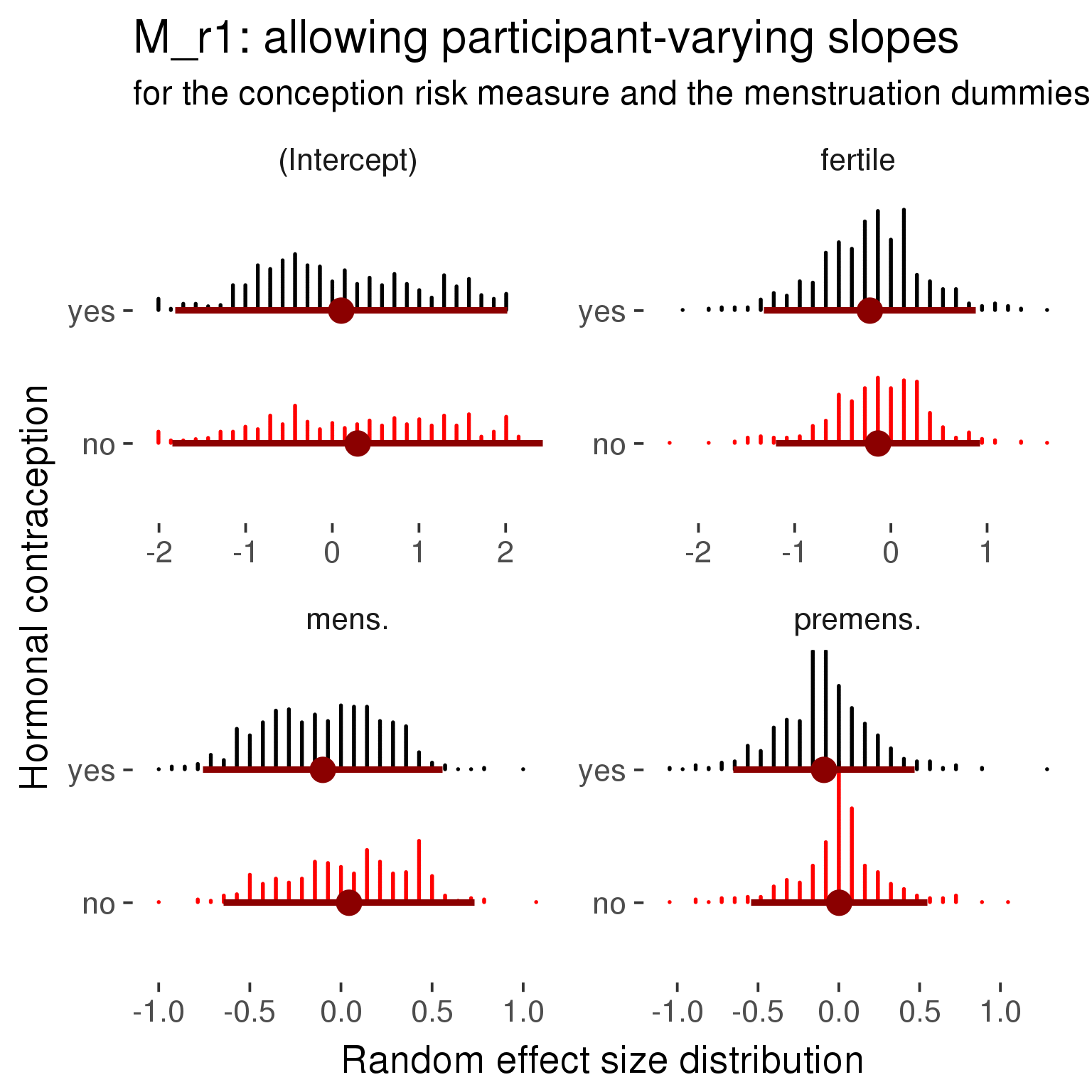
Generalized linear mixed model fit by maximum likelihood (Laplace Approximation) ['glmerMod']
Family: binomial ( probit )
Formula: spent_night_with_partner ~ included + menstruation + fertile +
fertile_mean + (1 + fertile + menstruation | person) + included:menstruation + included:fertile
Data: diary
AIC BIC logLik deviance df.resid
26740 26896 -13351 26702 26685
Scaled residuals:
Min 1Q Median 3Q Max
-4.816 -0.575 0.124 0.487 4.597
Random effects:
Groups Name Variance Std.Dev. Corr
person (Intercept) 1.420 1.192
fertile 1.233 1.110 0.02
menstruationpre 0.322 0.567 -0.13 0.28
menstruationyes 0.355 0.596 0.31 0.21 0.59
Number of obs: 26704, groups: person, 1054
Fixed effects:
Estimate Std. Error z value Pr(>|z|)
(Intercept) 0.329580 0.000234 1411 <2e-16 ***
includedhorm_contra -0.208214 0.000241 -863 <2e-16 ***
menstruationpre 0.004434 0.000234 19 <2e-16 ***
menstruationyes 0.055668 0.000234 238 <2e-16 ***
fertile -0.127744 0.000241 -530 <2e-16 ***
fertile_mean 0.480269 0.000241 1991 <2e-16 ***
includedhorm_contra:menstruationpre -0.097614 0.000234 -418 <2e-16 ***
includedhorm_contra:menstruationyes -0.152652 0.000241 -633 <2e-16 ***
includedhorm_contra:fertile -0.089222 0.000234 -382 <2e-16 ***
---
Signif. codes: 0 '***' 0.001 '**' 0.01 '*' 0.05 '.' 0.1 ' ' 1
Correlation of Fixed Effects:
(Intr) incld_ mnstrtnp mnstrtny fertil frtl_m inclddhrm_cntr:mnstrtnp
inclddhrm_c 0.000
menstrutnpr 0.000 0.000
menstrutnys 0.000 0.000 0.000
fertile 0.000 0.000 0.000 0.000
fertile_men 0.000 0.000 0.000 0.000 0.000
inclddhrm_cntr:mnstrtnp 0.000 0.000 0.000 0.000 0.000 0.000
inclddhrm_cntr:mnstrtny 0.000 0.000 0.000 0.000 0.250 0.000 0.000
inclddhrm_cntr:f 0.000 0.000 0.000 0.000 0.000 0.000 0.000
inclddhrm_cntr:mnstrtny
inclddhrm_c
menstrutnpr
menstrutnys
fertile
fertile_men
inclddhrm_cntr:mnstrtnp
inclddhrm_cntr:mnstrtny
inclddhrm_cntr:f 0.000
convergence code: 0
Model failed to converge with max|grad| = 0.380892 (tol = 0.001, component 1)
Model is nearly unidentifiable: very large eigenvalue
- Rescale variables?
| Df | AIC | BIC | logLik | deviance | Chisq | Chi Df | Pr(>Chisq) | |
|---|---|---|---|---|---|---|---|---|
| model | 10 | 26976 | 27058 | -13478 | 26956 | NA | NA | NA |
| with_ind_diff | 19 | 26740 | 26896 | -13351 | 26702 | 253.8 | 9 | 1.611e-49 |
robustness_check_ovu_shift(model, diary)M_e: Exclusion criteria
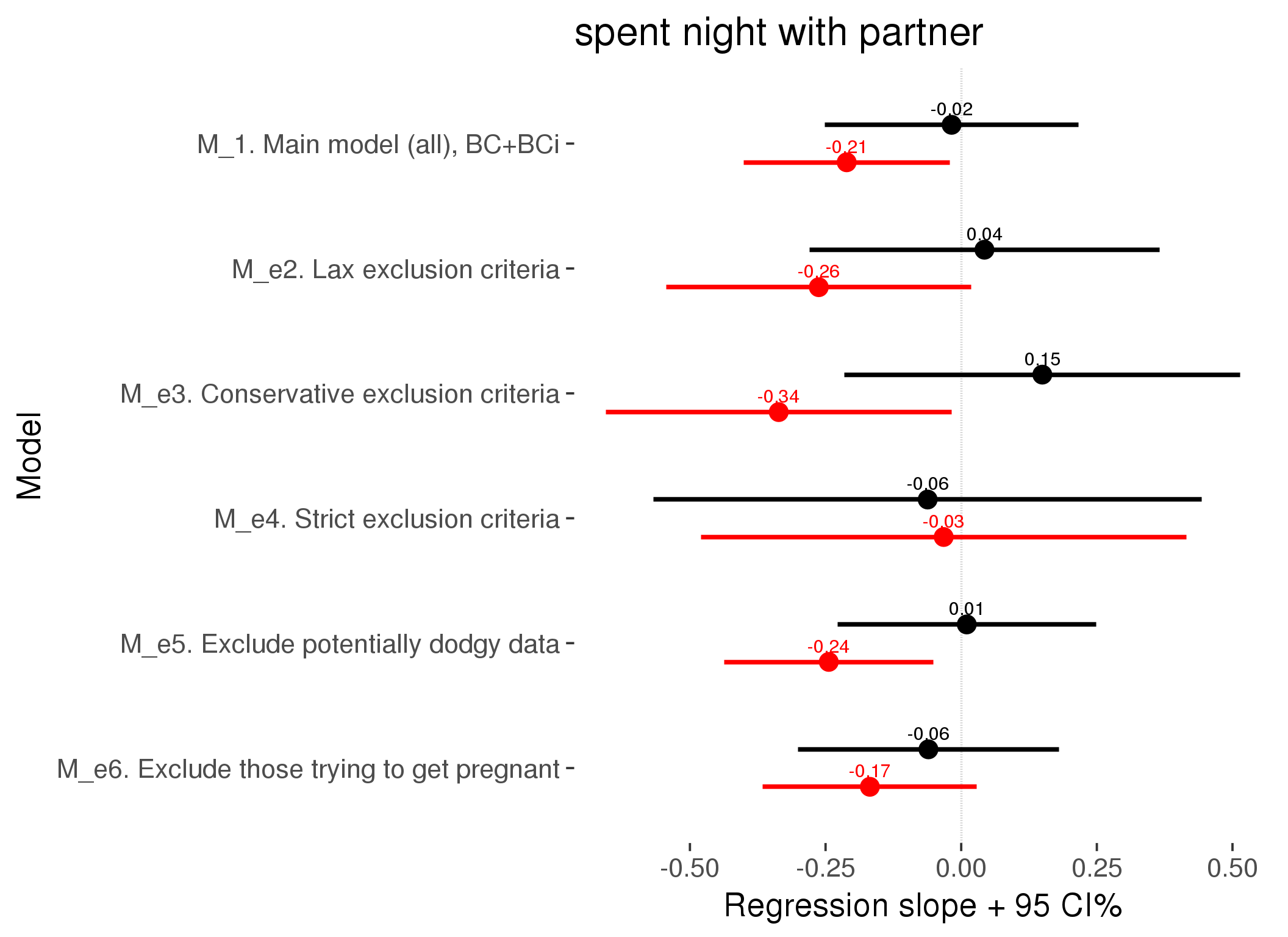
M_p: Predictors
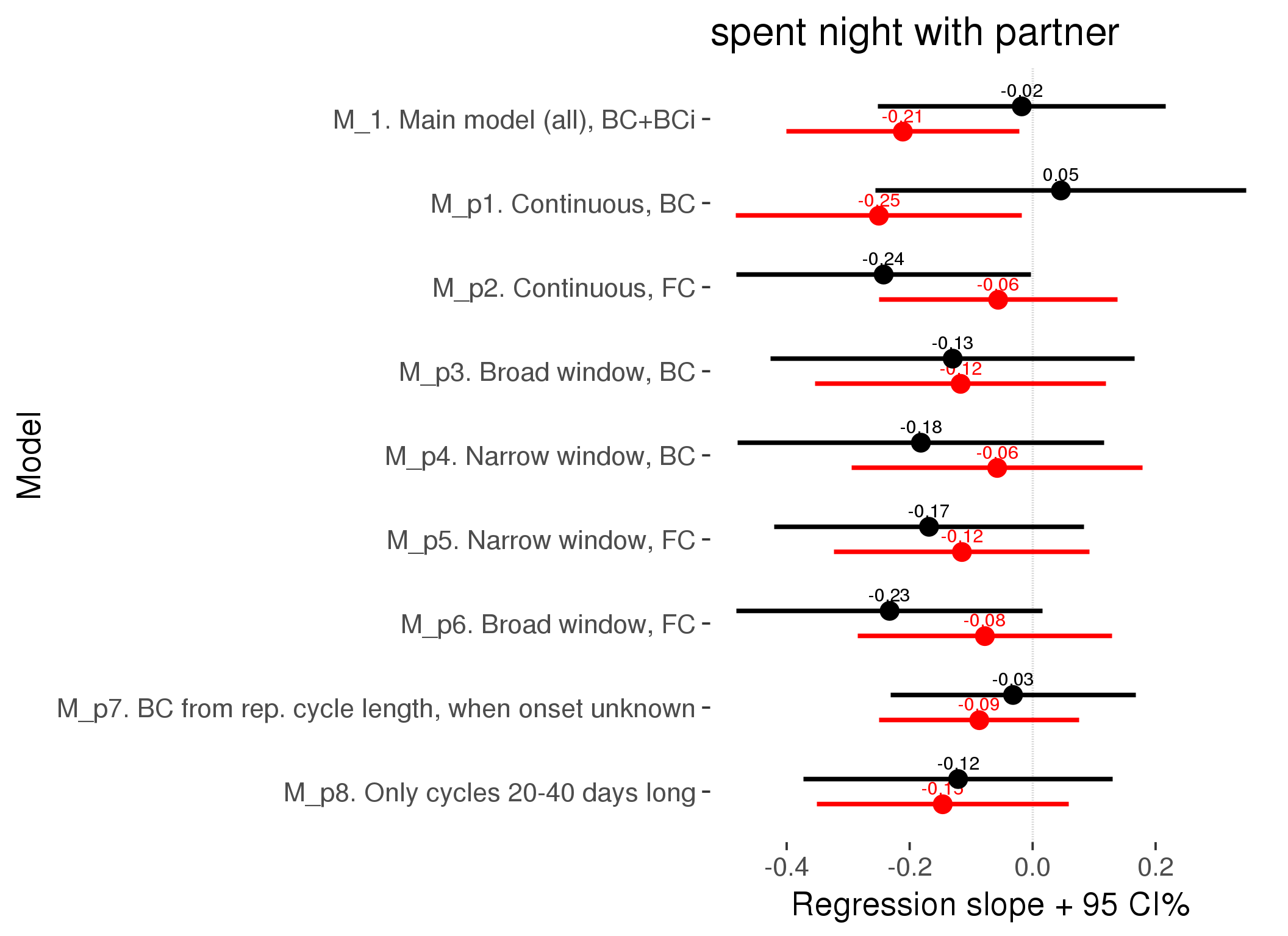
M_c: Covariates, controls, autocorrelation
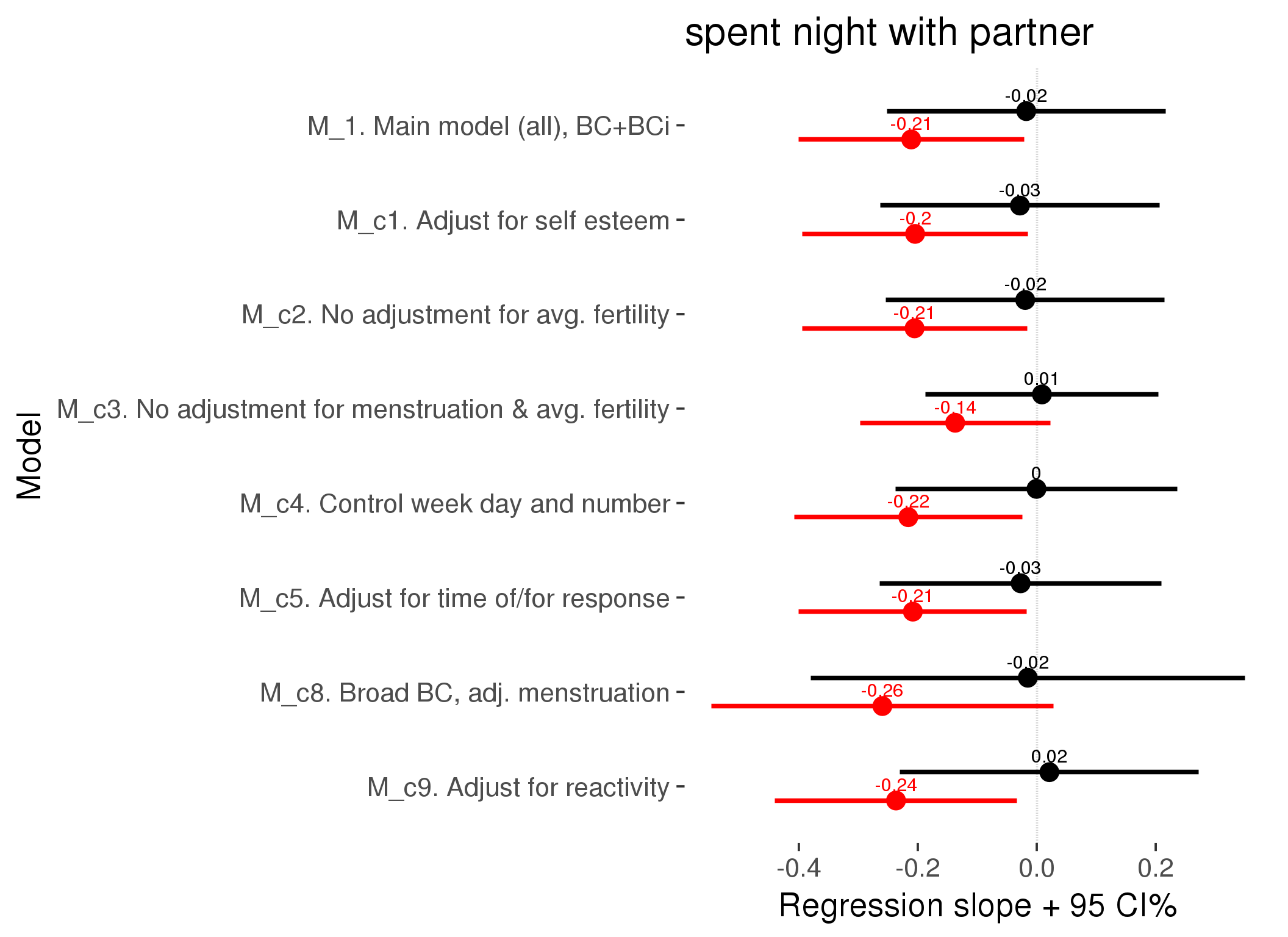
Generalized linear mixed model fit by maximum likelihood (Laplace Approximation) ['glmerMod']
Family: binomial ( probit )
AIC BIC logLik deviance df.resid
24516 24662 -12240 24480 24380
Scaled residuals:
Min 1Q Median 3Q Max
-5.450 -0.601 0.124 0.505 5.045
Random effects:
Groups Name Variance Std.Dev.
person (Intercept) 1.4885547003 1.220063
Xr.2 s(days_filled_out):includedhorm_contra 0.0000001306 0.000361
Xr.1 s(days_filled_out):includedcycling 0.0000025894 0.001609
Xr.0 s(day_number):includedhorm_contra 0.0056527989 0.075185
Xr s(day_number):includedcycling 0.0000000274 0.000166
Number of obs: 24398, groups: person, 1054; Xr.2, 8; Xr.1, 8; Xr.0, 8; Xr, 8
Fixed effects:
Estimate Std. Error z value Pr(>|z|)
X(Intercept) 0.34745 0.11107 3.13 0.00176 **
Xincludedhorm_contra -0.23760 0.09059 -2.62 0.00872 **
Xmenstruationpre 0.00979 0.05017 0.20 0.84527
Xmenstruationyes -0.03610 0.04864 -0.74 0.45798
Xfertile -0.23661 0.10394 -2.28 0.02283 *
Xfertile_mean 0.45678 0.50971 0.90 0.37017
Xincludedhorm_contra:menstruationpre -0.08630 0.06263 -1.38 0.16824
Xincludedhorm_contra:menstruationyes -0.09885 0.06185 -1.60 0.11001
Xincludedhorm_contra:fertile 0.02121 0.12828 0.17 0.86867
Xs(day_number):includedcyclingFx1 0.05743 0.08053 0.71 0.47575
Xs(day_number):includedhorm_contraFx1 0.36189 0.09850 3.67 0.00024 ***
Xs(days_filled_out):includedcyclingFx1 0.01454 0.08301 0.18 0.86098
Xs(days_filled_out):includedhorm_contraFx1 -0.32875 0.06748 -4.87 0.0000011 ***
---
Signif. codes: 0 '***' 0.001 '**' 0.01 '*' 0.05 '.' 0.1 ' ' 1
Family: binomial
Link function: probit
Formula:
spent_night_with_partner ~ included + menstruation + fertile +
fertile_mean + s(day_number, by = included) + s(days_filled_out,
by = included) + included:menstruation + included:fertile
Parametric coefficients:
Estimate Std. Error z value Pr(>|z|)
(Intercept) 0.34745 0.10803 3.22 0.0013 **
includedhorm_contra -0.23760 0.08962 -2.65 0.0080 **
menstruationpre 0.00979 0.05009 0.20 0.8450
menstruationyes -0.03610 0.04810 -0.75 0.4530
fertile -0.23661 0.10305 -2.30 0.0217 *
fertile_mean 0.45678 0.48993 0.93 0.3512
includedhorm_contra:menstruationpre -0.08630 0.06238 -1.38 0.1665
includedhorm_contra:menstruationyes -0.09885 0.06111 -1.62 0.1057
includedhorm_contra:fertile 0.02121 0.12712 0.17 0.8675
---
Signif. codes: 0 '***' 0.001 '**' 0.01 '*' 0.05 '.' 0.1 ' ' 1
Approximate significance of smooth terms:
edf Ref.df Chi.sq p-value
s(day_number):includedcycling 1.00 1.00 0.52 0.47
s(day_number):includedhorm_contra 1.88 1.88 25.86 0.00000158 ***
s(days_filled_out):includedcycling 1.00 1.00 0.03 0.86
s(days_filled_out):includedhorm_contra 1.00 1.00 24.58 0.00000071 ***
---
Signif. codes: 0 '***' 0.001 '**' 0.01 '*' 0.05 '.' 0.1 ' ' 1
R-sq.(adj) = 0.00968
glmer.ML = 21064 Scale est. = 1 n = 24398
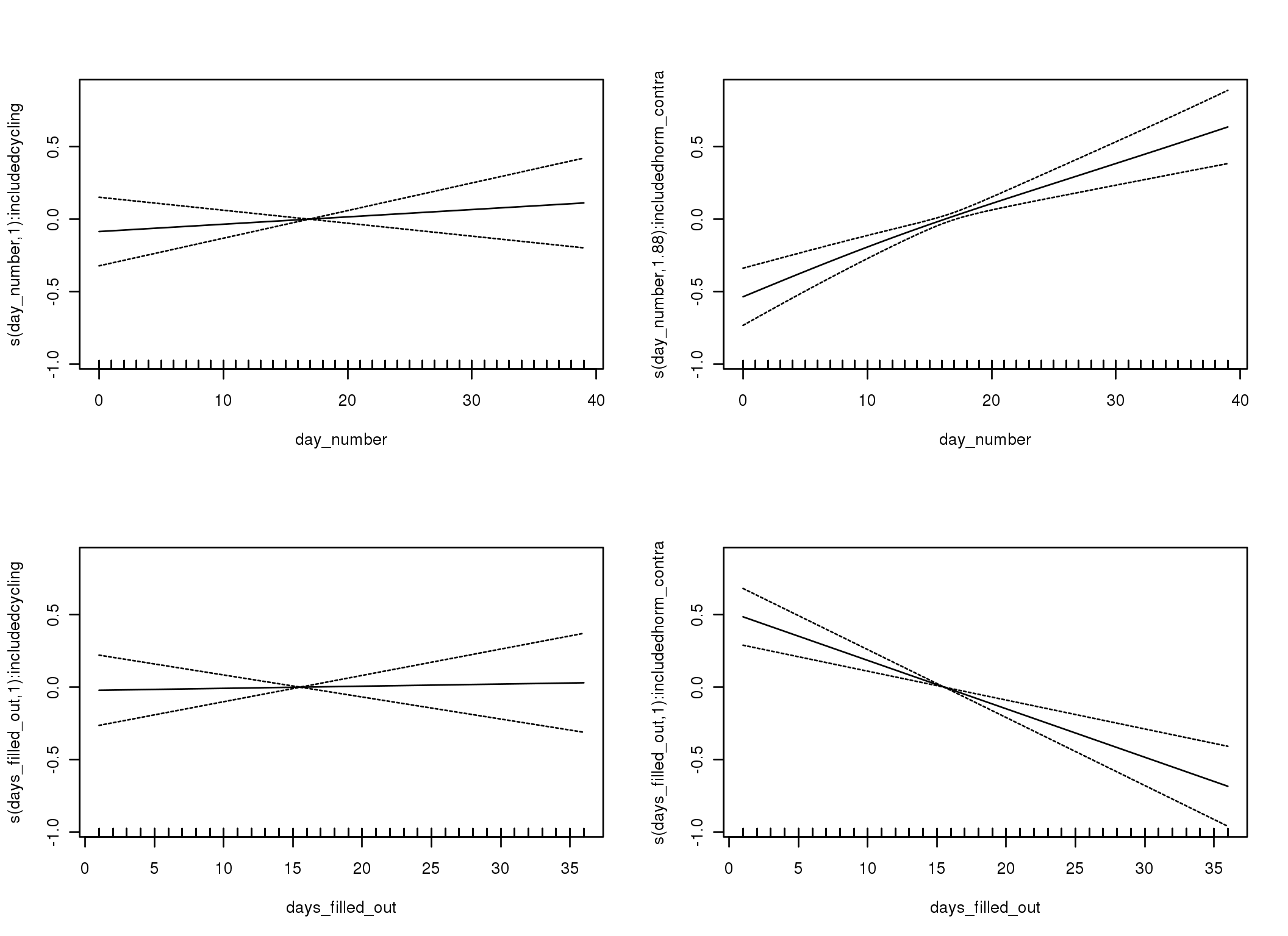
M_d: Other designs
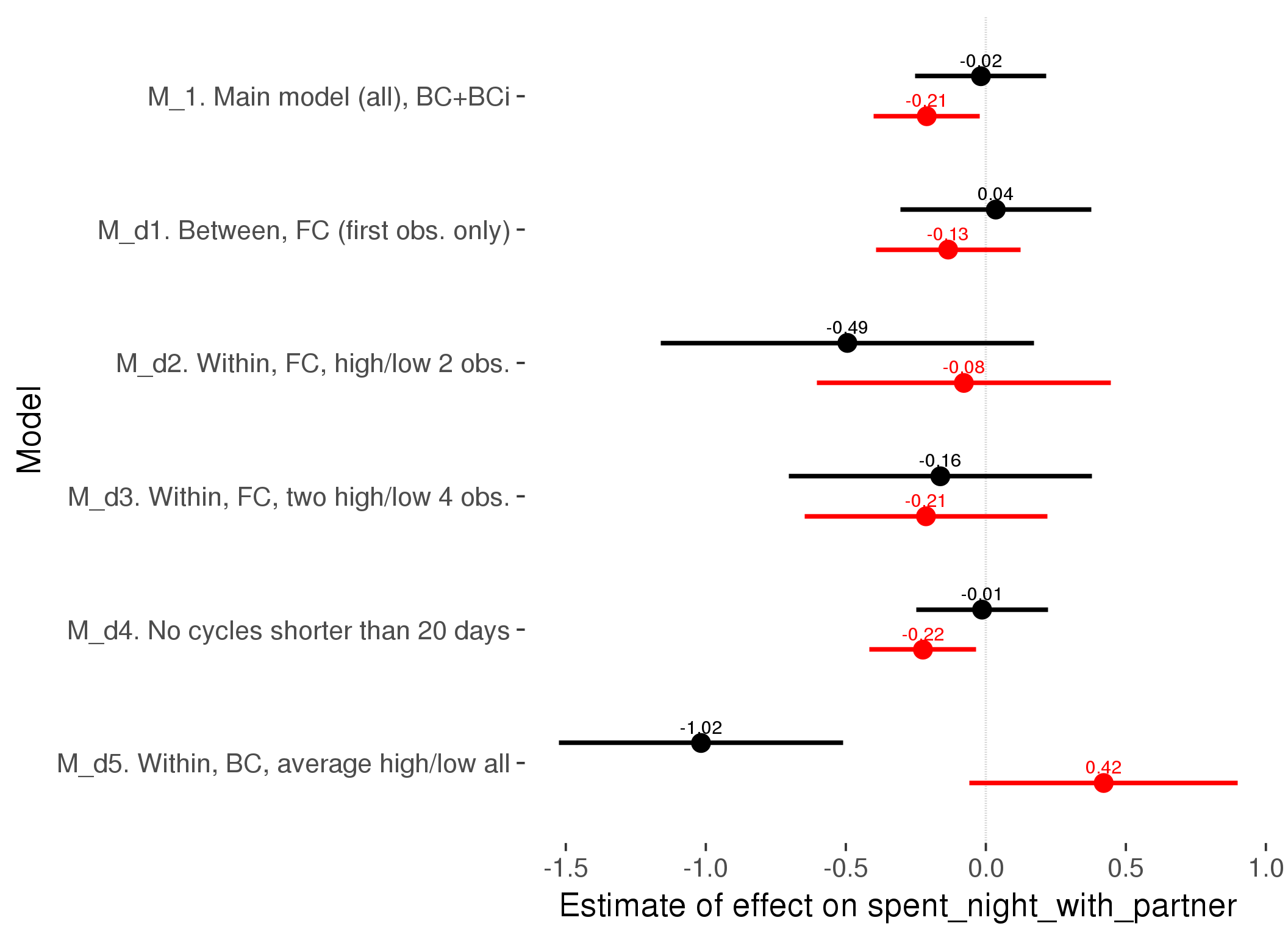
M_m1: Moderation by contraceptive method
Based on the sample with lax exclusion criteria. Users who used any hormonal contraception are classified as hormonal, users who use any awareness-based methods (counting, temperature-based) are classified as ‘fertility-awareness’, women who don’t fall into the before groups and use condoms, pessars, coitus interruptus etc. are classified as ‘barrie or abstinence’. Women who don’t use contraception or use other methods such as sterilisation are excluded from this analysis.
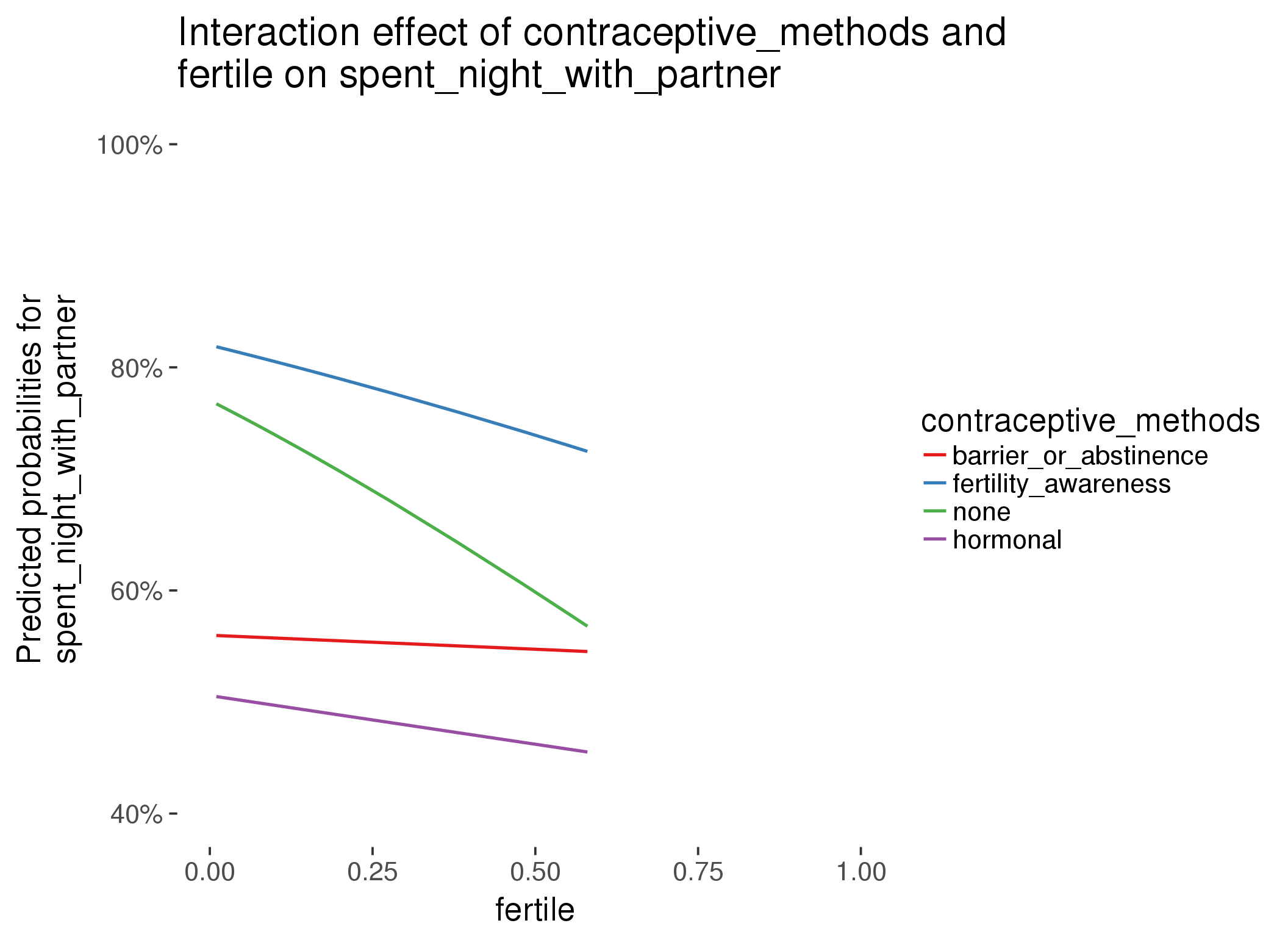
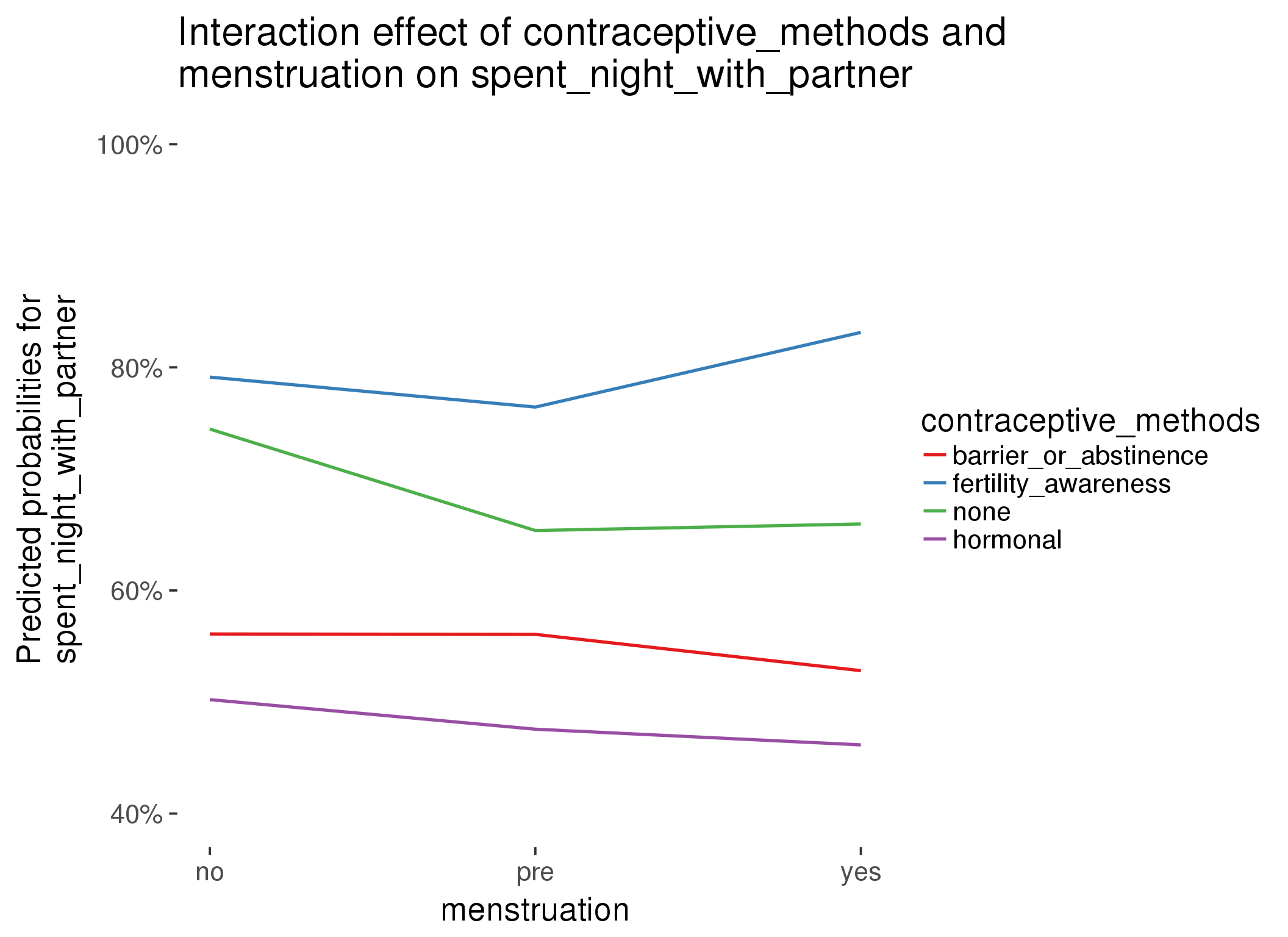
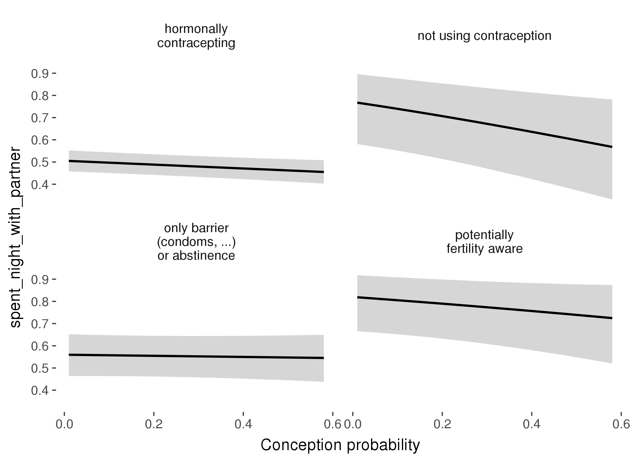
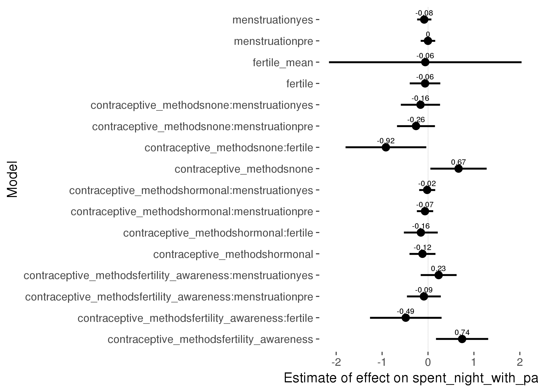
Generalized linear mixed model fit by maximum likelihood (Laplace Approximation) ['glmerMod']
Family: binomial ( probit )
Formula: spent_night_with_partner ~ fertile_mean + (1 | person) + contraceptive_methods +
fertile + menstruation + fertile:contraceptive_methods + menstruation:contraceptive_methods
Data: diary
Subset: !is.na(included_lax) & contraceptive_method != "other"
AIC BIC logLik deviance df.resid
17622 17761 -8793 17586 17026
Scaled residuals:
Min 1Q Median 3Q Max
-6.192 -0.611 0.100 0.544 4.796
Random effects:
Groups Name Variance Std.Dev.
person (Intercept) 1.23 1.11
Number of obs: 17044, groups: person, 513
Fixed effects:
Estimate Std. Error z value Pr(>|z|)
(Intercept) 0.174997 0.219170 0.80 0.425
fertile_mean -0.059503 1.070161 -0.06 0.956
contraceptive_methodsfertility_awareness 0.742423 0.289258 2.57 0.010 *
contraceptive_methodsnone 0.665232 0.312021 2.13 0.033 *
contraceptive_methodshormonal -0.120870 0.143356 -0.84 0.399
fertile -0.063555 0.170508 -0.37 0.709
menstruationpre -0.000916 0.081605 -0.01 0.991
menstruationyes -0.082980 0.078595 -1.06 0.291
contraceptive_methodsfertility_awareness:fertile -0.485124 0.397305 -1.22 0.222
contraceptive_methodsnone:fertile -0.917383 0.448719 -2.04 0.041 *
contraceptive_methodshormonal:fertile -0.155423 0.188654 -0.82 0.410
contraceptive_methodsfertility_awareness:menstruationpre -0.089324 0.187744 -0.48 0.634
contraceptive_methodsnone:menstruationpre -0.261479 0.210927 -1.24 0.215
contraceptive_methodshormonal:menstruationpre -0.065553 0.091008 -0.72 0.471
contraceptive_methodsfertility_awareness:menstruationyes 0.231796 0.199884 1.16 0.246
contraceptive_methodsnone:menstruationyes -0.163421 0.218253 -0.75 0.454
contraceptive_methodshormonal:menstruationyes -0.018851 0.088643 -0.21 0.832
---
Signif. codes: 0 '***' 0.001 '**' 0.01 '*' 0.05 '.' 0.1 ' ' 1
convergence code: 0
Model failed to converge with max|grad| = 0.00431976 (tol = 0.001, component 1)
| Df | AIC | BIC | logLik | deviance | Chisq | Chi Df | Pr(>Chisq) | |
|---|---|---|---|---|---|---|---|---|
| add_main | 12 | 17618 | 17711 | -8797 | 17594 | NA | NA | NA |
| by_method | 18 | 17622 | 17761 | -8793 | 17586 | 8.329 | 6 | 0.215 |
M_m2: Moderation by participant age
model %>%
test_moderator("age_group", diary, xlevels = 5)| Df | AIC | BIC | logLik | deviance | Chisq | Chi Df | Pr(>Chisq) | |
|---|---|---|---|---|---|---|---|---|
| with_main | 18 | 26885 | 27033 | -13425 | 26849 | NA | NA | NA |
| with_mod | 26 | 26893 | 27106 | -13421 | 26841 | 8.017 | 8 | 0.4318 |
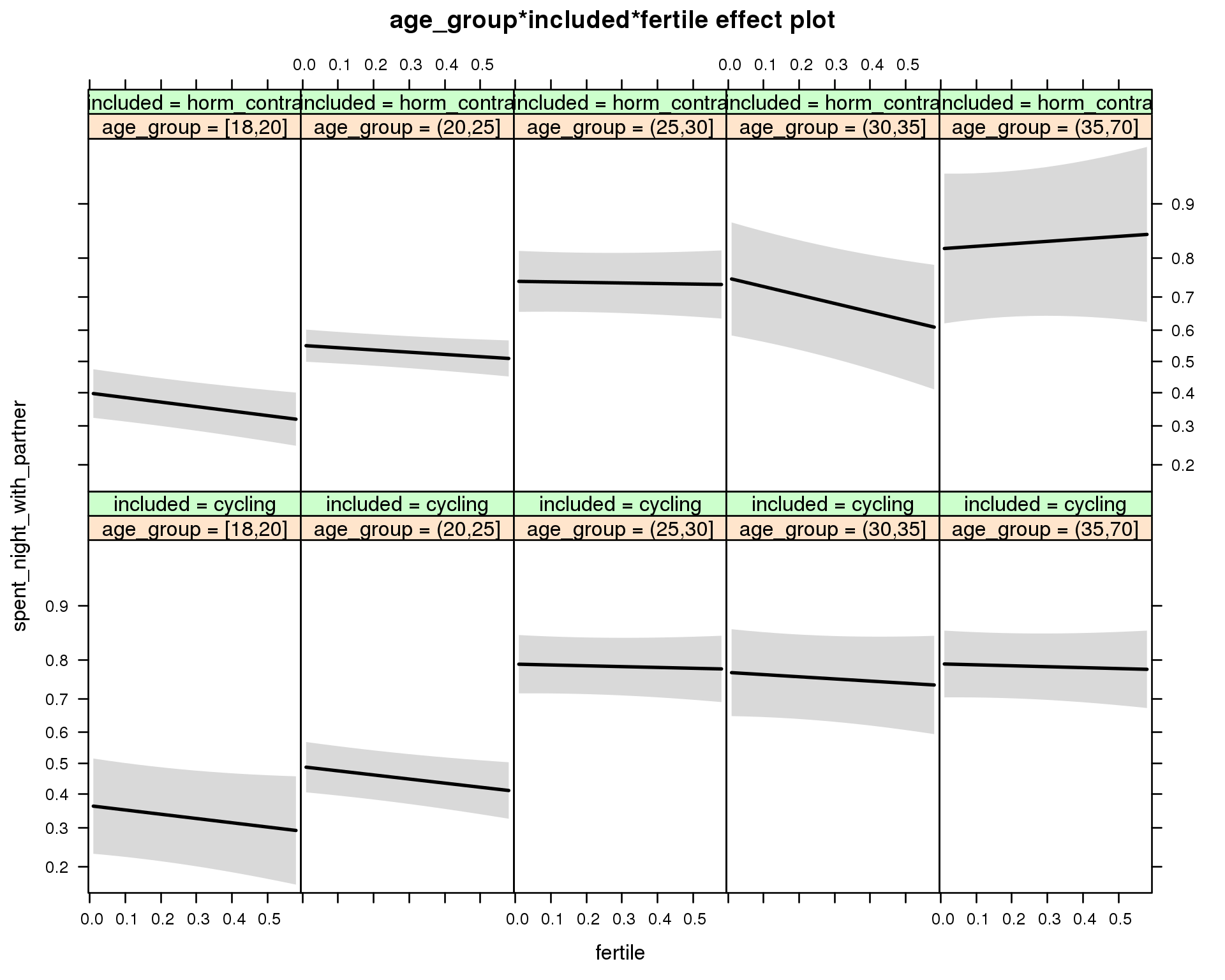
Generalized linear mixed model fit by maximum likelihood (Laplace Approximation) ['glmerMod']
Family: binomial ( probit )
Formula: spent_night_with_partner ~ menstruation + fertile_mean + (1 |
person) + age_group + included + fertile + menstruation:included +
age_group:included + age_group:fertile + included:fertile + age_group:included:fertile
Data: diary
AIC BIC logLik deviance df.resid
26893 27106 -13421 26841 26678
Scaled residuals:
Min 1Q Median 3Q Max
-5.390 -0.599 0.124 0.513 5.074
Random effects:
Groups Name Variance Std.Dev.
person (Intercept) 1.25 1.12
Number of obs: 26704, groups: person, 1054
Fixed effects:
Estimate Std. Error z value Pr(>|z|)
(Intercept) -0.3943 0.2108 -1.87 0.061 .
menstruationpre -0.0214 0.0477 -0.45 0.654
menstruationyes -0.0220 0.0454 -0.49 0.627
fertile_mean 0.3167 0.4779 0.66 0.507
age_group(20,25] 0.3171 0.2241 1.41 0.157
age_group(25,30] 1.1532 0.2323 4.96 0.00000069 ***
age_group(30,35] 1.0855 0.2683 4.05 0.00005203 ***
age_group(35,70] 1.1551 0.2417 4.78 0.00000176 ***
includedhorm_contra 0.1172 0.2244 0.52 0.602
fertile -0.3473 0.2602 -1.33 0.182
menstruationpre:includedhorm_contra -0.0664 0.0596 -1.11 0.265
menstruationyes:includedhorm_contra -0.0958 0.0577 -1.66 0.097 .
age_group(20,25]:includedhorm_contra 0.0708 0.2550 0.28 0.781
age_group(25,30]:includedhorm_contra -0.2428 0.2834 -0.86 0.392
age_group(30,35]:includedhorm_contra -0.1491 0.3710 -0.40 0.688
age_group(35,70]:includedhorm_contra 0.0207 0.4077 0.05 0.960
age_group(20,25]:fertile 0.0142 0.2881 0.05 0.961
age_group(25,30]:fertile 0.2800 0.3062 0.91 0.361
age_group(30,35]:fertile 0.1712 0.3608 0.47 0.635
age_group(35,70]:fertile 0.2712 0.3260 0.83 0.406
includedhorm_contra:fertile -0.0189 0.2869 -0.07 0.947
age_group(20,25]:includedhorm_contra:fertile 0.1699 0.3206 0.53 0.596
age_group(25,30]:includedhorm_contra:fertile 0.0417 0.3682 0.11 0.910
age_group(30,35]:includedhorm_contra:fertile -0.4930 0.4923 -1.00 0.317
age_group(35,70]:includedhorm_contra:fertile 0.2961 0.5950 0.50 0.619
---
Signif. codes: 0 '***' 0.001 '**' 0.01 '*' 0.05 '.' 0.1 ' ' 1
convergence code: 0
Model failed to converge with max|grad| = 0.068793 (tol = 0.001, component 1)
M_m3: Moderation by weekend
model %>%
test_moderator("weekend", diary, xlevels = 2) | Df | AIC | BIC | logLik | deviance | Chisq | Chi Df | Pr(>Chisq) | |
|---|---|---|---|---|---|---|---|---|
| with_main | 12 | 26753 | 26852 | -13365 | 26729 | NA | NA | NA |
| with_mod | 14 | 26757 | 26872 | -13364 | 26729 | 0.4693 | 2 | 0.7908 |
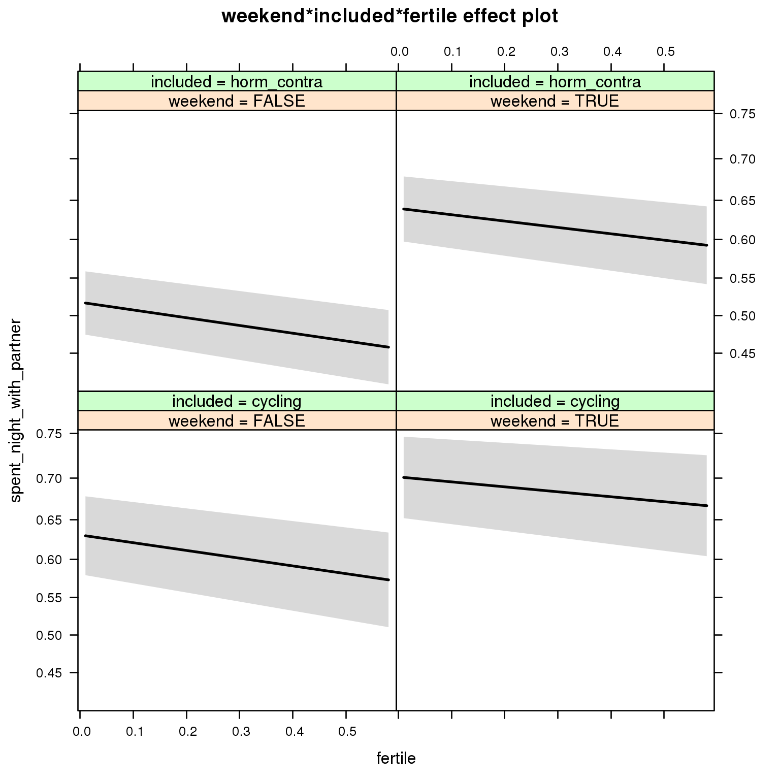
Generalized linear mixed model fit by maximum likelihood (Laplace Approximation) ['glmerMod']
Family: binomial ( probit )
Formula: spent_night_with_partner ~ menstruation + fertile_mean + (1 |
person) + weekend + included + fertile + menstruation:included +
weekend:included + weekend:fertile + included:fertile + weekend:included:fertile
Data: diary
AIC BIC logLik deviance df.resid
26757 26872 -13364 26729 26690
Scaled residuals:
Min 1Q Median 3Q Max
-6.552 -0.585 0.128 0.522 4.900
Random effects:
Groups Name Variance Std.Dev.
person (Intercept) 1.43 1.2
Number of obs: 26704, groups: person, 1054
Fixed effects:
Estimate Std. Error z value Pr(>|z|)
(Intercept) 0.267853 0.109759 2.44 0.0147 *
menstruationpre -0.021907 0.047802 -0.46 0.6467
menstruationyes -0.022255 0.045475 -0.49 0.6246
fertile_mean 0.431111 0.500255 0.86 0.3888
weekendTRUE 0.193996 0.041656 4.66 0.0000032 ***
includedhorm_contra -0.261639 0.090230 -2.90 0.0037 **
fertile -0.258494 0.118512 -2.18 0.0292 *
menstruationpre:includedhorm_contra -0.070648 0.059781 -1.18 0.2373
menstruationyes:includedhorm_contra -0.094946 0.057952 -1.64 0.1014
weekendTRUE:includedhorm_contra 0.119699 0.052298 2.29 0.0221 *
weekendTRUE:fertile 0.092828 0.162159 0.57 0.5670
includedhorm_contra:fertile -0.000317 0.147166 0.00 0.9983
weekendTRUE:includedhorm_contra:fertile -0.046468 0.200976 -0.23 0.8172
---
Signif. codes: 0 '***' 0.001 '**' 0.01 '*' 0.05 '.' 0.1 ' ' 1
convergence code: 0
Model failed to converge with max|grad| = 0.00722533 (tol = 0.001, component 1)
M_m4: Moderation by weekday
model %>%
test_moderator("weekday", diary, xlevels = 7)| Df | AIC | BIC | logLik | deviance | Chisq | Chi Df | Pr(>Chisq) | |
|---|---|---|---|---|---|---|---|---|
| with_main | 22 | 26502 | 26682 | -13229 | 26458 | NA | NA | NA |
| with_mod | 34 | 26524 | 26802 | -13228 | 26456 | 2.11 | 12 | 0.9992 |
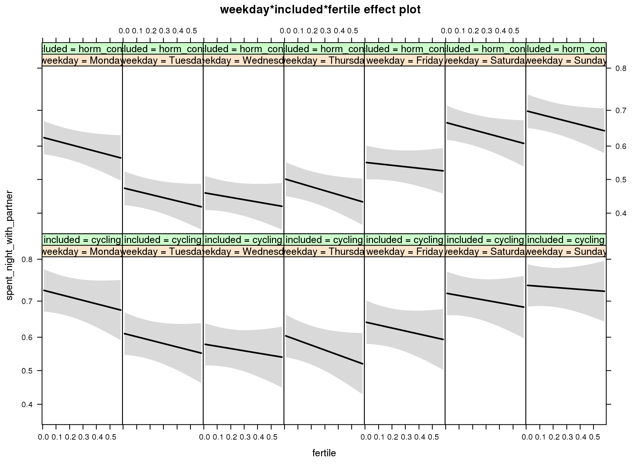
Generalized linear mixed model fit by maximum likelihood (Laplace Approximation) ['glmerMod']
Family: binomial ( probit )
Formula: spent_night_with_partner ~ menstruation + fertile_mean + (1 |
person) + weekday + included + fertile + menstruation:included +
weekday:included + weekday:fertile + included:fertile + weekday:included:fertile
Data: diary
AIC BIC logLik deviance df.resid
26524 26802 -13228 26456 26670
Scaled residuals:
Min 1Q Median 3Q Max
-7.383 -0.572 0.125 0.515 5.194
Random effects:
Groups Name Variance Std.Dev.
person (Intercept) 1.47 1.21
Number of obs: 26704, groups: person, 1054
Fixed effects:
Estimate Std. Error z value Pr(>|z|)
(Intercept) 0.547274 0.120444 4.54 0.000005524 ***
menstruationpre -0.026196 0.048077 -0.54 0.5858
menstruationyes -0.025173 0.045725 -0.55 0.5820
fertile_mean 0.405252 0.505994 0.80 0.4232
weekdayTuesday -0.326816 0.075399 -4.33 0.000014609 ***
weekdayWednesday -0.408330 0.075601 -5.40 0.000000066 ***
weekdayThursday -0.342503 0.076034 -4.50 0.000006650 ***
weekdayFriday -0.241542 0.077313 -3.12 0.0018 **
weekdaySaturday -0.023595 0.077862 -0.30 0.7619
weekdaySunday 0.035873 0.075333 0.48 0.6339
includedhorm_contra -0.261361 0.107936 -2.42 0.0155 *
fertile -0.260817 0.215588 -1.21 0.2264
menstruationpre:includedhorm_contra -0.065983 0.060144 -1.10 0.2726
menstruationyes:includedhorm_contra -0.092729 0.058287 -1.59 0.1116
weekdayTuesday:includedhorm_contra -0.055489 0.094761 -0.59 0.5582
weekdayWednesday:includedhorm_contra -0.010175 0.095325 -0.11 0.9150
weekdayThursday:includedhorm_contra 0.029173 0.095678 0.30 0.7604
weekdayFriday:includedhorm_contra 0.052100 0.096588 0.54 0.5896
weekdaySaturday:includedhorm_contra 0.135811 0.097298 1.40 0.1628
weekdaySunday:includedhorm_contra 0.163875 0.094376 1.74 0.0825 .
weekdayTuesday:fertile 0.002694 0.294474 0.01 0.9927
weekdayWednesday:fertile 0.091341 0.297630 0.31 0.7589
weekdayThursday:fertile -0.108871 0.299829 -0.36 0.7165
weekdayFriday:fertile 0.033804 0.299551 0.11 0.9102
weekdaySaturday:fertile 0.079304 0.302834 0.26 0.7934
weekdaySunday:fertile 0.182962 0.295691 0.62 0.5361
includedhorm_contra:fertile -0.007453 0.267026 -0.03 0.9777
weekdayTuesday:includedhorm_contra:fertile 0.019895 0.366803 0.05 0.9567
weekdayWednesday:includedhorm_contra:fertile 0.000466 0.371336 0.00 0.9990
weekdayThursday:includedhorm_contra:fertile 0.077201 0.372427 0.21 0.8358
weekdayFriday:includedhorm_contra:fertile 0.124318 0.370937 0.34 0.7375
weekdaySaturday:includedhorm_contra:fertile -0.083707 0.374559 -0.22 0.8232
weekdaySunday:includedhorm_contra:fertile -0.173774 0.365606 -0.48 0.6346
---
Signif. codes: 0 '***' 0.001 '**' 0.01 '*' 0.05 '.' 0.1 ' ' 1
convergence code: 0
Model failed to converge with max|grad| = 0.0397336 (tol = 0.001, component 1)
failure to converge in 10000 evaluations
M_m5: Moderation by exclusion threshold
model %>%
test_moderator("included_levels", diary, xlevels = 4)| Df | AIC | BIC | logLik | deviance | Chisq | Chi Df | Pr(>Chisq) | |
|---|---|---|---|---|---|---|---|---|
| with_main | 16 | 26964 | 27095 | -13466 | 26932 | NA | NA | NA |
| with_mod | 22 | 26970 | 27150 | -13463 | 26926 | 6.366 | 6 | 0.3835 |
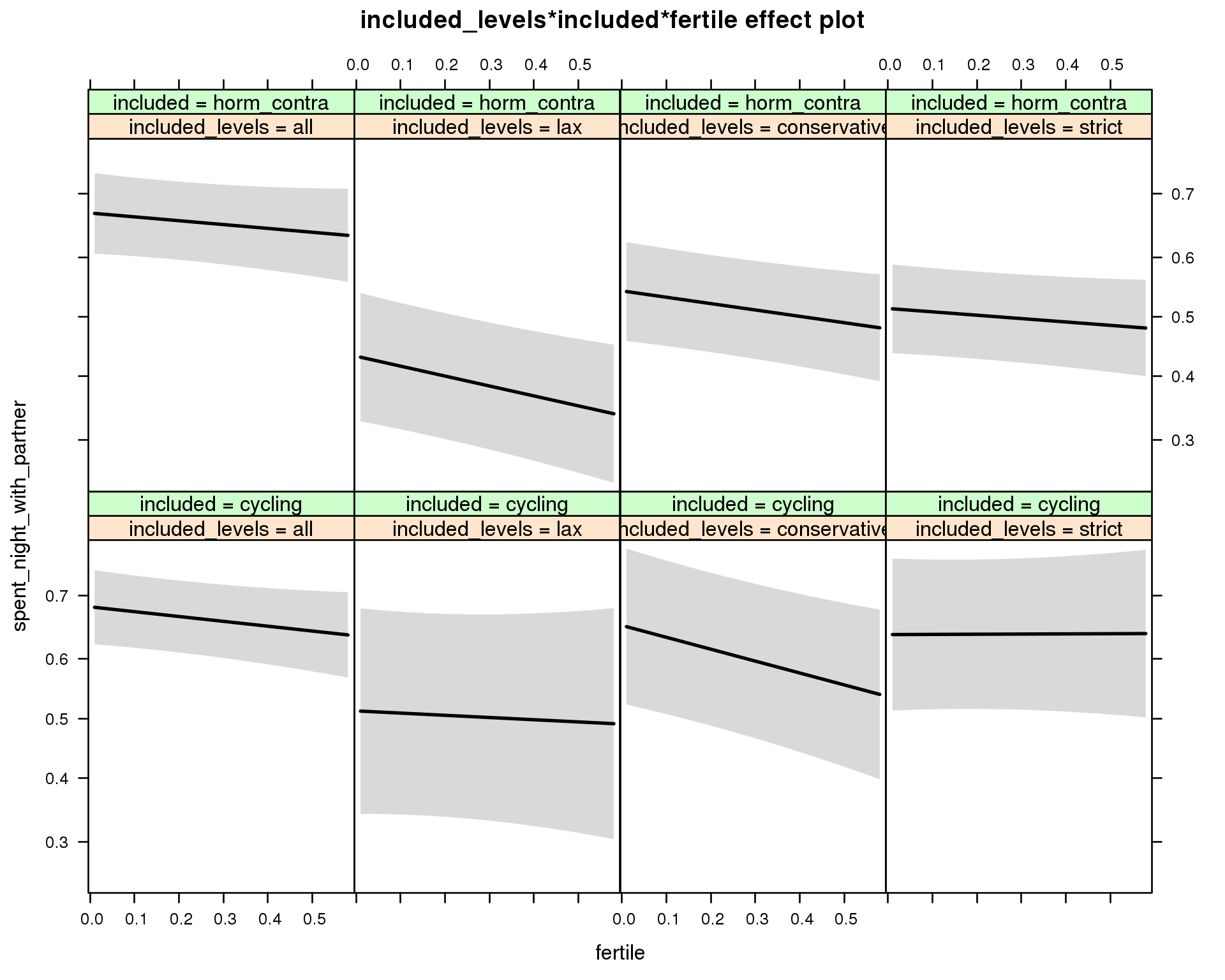
Generalized linear mixed model fit by maximum likelihood (Laplace Approximation) ['glmerMod']
Family: binomial ( probit )
Formula: spent_night_with_partner ~ menstruation + fertile_mean + (1 |
person) + included_levels + included + fertile + menstruation:included +
included_levels:included + included_levels:fertile + included:fertile +
included_levels:included:fertile
Data: diary
AIC BIC logLik deviance df.resid
26970 27150 -13463 26926 26682
Scaled residuals:
Min 1Q Median 3Q Max
-5.363 -0.600 0.129 0.515 5.206
Random effects:
Groups Name Variance Std.Dev.
person (Intercept) 1.38 1.17
Number of obs: 26704, groups: person, 1054
Fixed effects:
Estimate Std. Error z value Pr(>|z|)
(Intercept) 0.40431 0.11854 3.41 0.00065 ***
menstruationpre -0.01876 0.04773 -0.39 0.69429
menstruationyes -0.02161 0.04538 -0.48 0.63393
fertile_mean 0.44980 0.49708 0.90 0.36553
included_levelslax -0.44320 0.23756 -1.87 0.06209 .
included_levelsconservative -0.07932 0.18769 -0.42 0.67258
included_levelsstrict -0.11816 0.18371 -0.64 0.52009
includedhorm_contra -0.00508 0.12164 -0.04 0.96671
fertile -0.20614 0.12259 -1.68 0.09264 .
menstruationpre:includedhorm_contra -0.06721 0.05965 -1.13 0.25980
menstruationyes:includedhorm_contra -0.09578 0.05782 -1.66 0.09763 .
included_levelslax:includedhorm_contra -0.16668 0.28967 -0.58 0.56500
included_levelsconservative:includedhorm_contra -0.25239 0.23353 -1.08 0.27981
included_levelsstrict:includedhorm_contra -0.28837 0.22519 -1.28 0.20036
included_levelslax:fertile 0.11223 0.29722 0.38 0.70573
included_levelsconservative:fertile -0.30023 0.22347 -1.34 0.17911
included_levelsstrict:fertile 0.21354 0.22390 0.95 0.34021
includedhorm_contra:fertile 0.04230 0.18091 0.23 0.81514
included_levelslax:includedhorm_contra:fertile -0.37115 0.35861 -1.03 0.30068
included_levelsconservative:includedhorm_contra:fertile 0.19307 0.28327 0.68 0.49549
included_levelsstrict:includedhorm_contra:fertile -0.19338 0.27827 -0.69 0.48709
---
Signif. codes: 0 '***' 0.001 '**' 0.01 '*' 0.05 '.' 0.1 ' ' 1
convergence code: 0
Model failed to converge with max|grad| = 0.0140053 (tol = 0.001, component 1)
M_m6: Moderation by cycle length
model %>%
test_moderator("cycle_length_groups", diary, xlevels = 4)| Df | AIC | BIC | logLik | deviance | Chisq | Chi Df | Pr(>Chisq) | |
|---|---|---|---|---|---|---|---|---|
| with_main | 16 | 26974 | 27105 | -13471 | 26942 | NA | NA | NA |
| with_mod | 22 | 26983 | 27163 | -13469 | 26939 | 3.649 | 6 | 0.7241 |
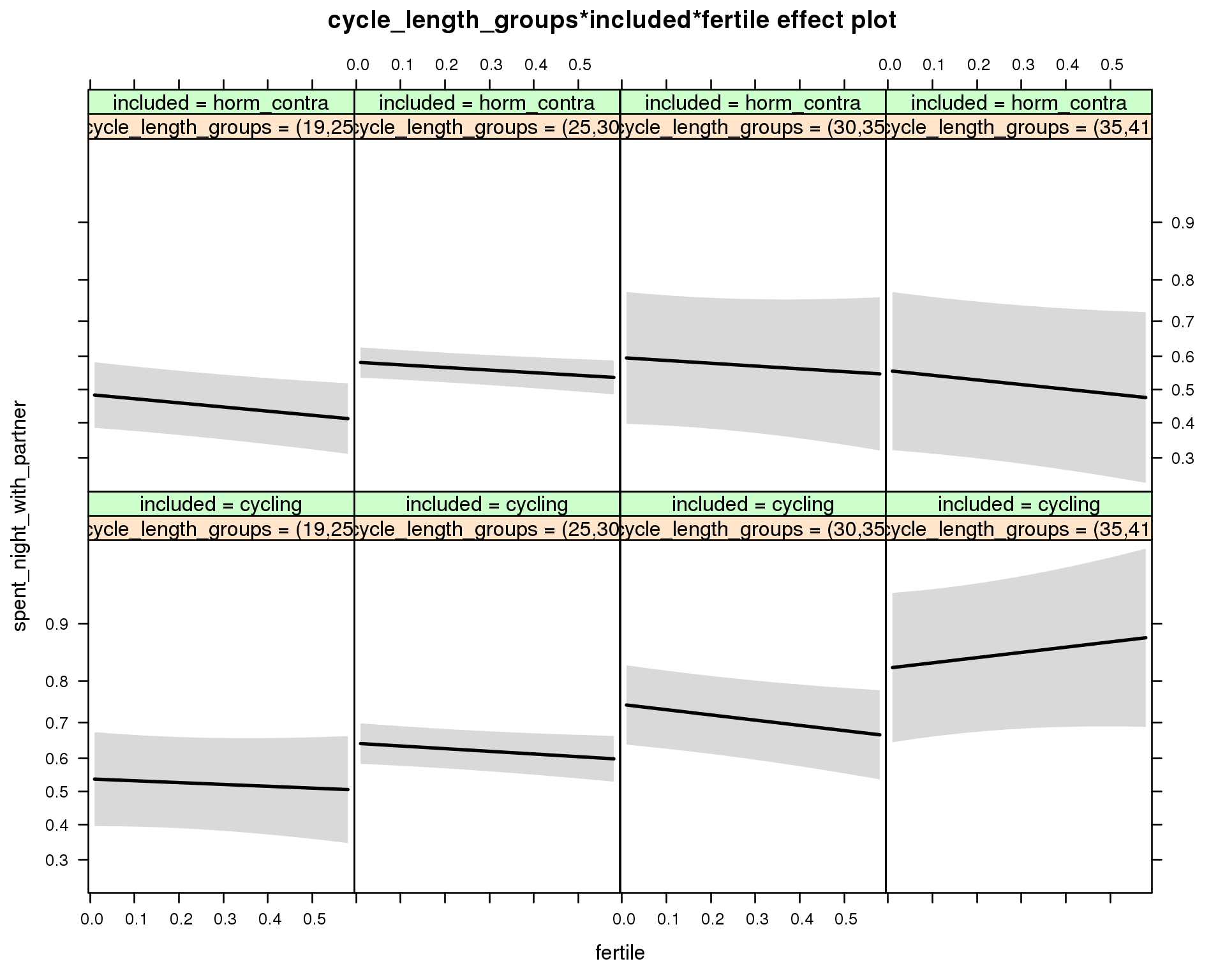
Generalized linear mixed model fit by maximum likelihood (Laplace Approximation) ['glmerMod']
Family: binomial ( probit )
Formula: spent_night_with_partner ~ menstruation + fertile_mean + (1 |
person) + cycle_length_groups + included + fertile + menstruation:included +
cycle_length_groups:included + cycle_length_groups:fertile +
included:fertile + cycle_length_groups:included:fertile
Data: diary
AIC BIC logLik deviance df.resid
26983 27163 -13469 26939 26682
Scaled residuals:
Min 1Q Median 3Q Max
-5.226 -0.599 0.127 0.516 4.816
Random effects:
Groups Name Variance Std.Dev.
person (Intercept) 1.39 1.18
Number of obs: 26704, groups: person, 1054
Fixed effects:
Estimate Std. Error z value Pr(>|z|)
(Intercept) -0.00423 0.20418 -0.02 0.983
menstruationpre -0.02007 0.04777 -0.42 0.674
menstruationyes -0.02135 0.04565 -0.47 0.640
fertile_mean 0.61207 0.50246 1.22 0.223
cycle_length_groups(25,30] 0.27276 0.20018 1.36 0.173
cycle_length_groups(30,35] 0.56996 0.24068 2.37 0.018 *
cycle_length_groups(35,41] 0.84873 0.34541 2.46 0.014 *
includedhorm_contra -0.10548 0.22578 -0.47 0.640
fertile -0.14070 0.27053 -0.52 0.603
menstruationpre:includedhorm_contra -0.06626 0.05966 -1.11 0.267
menstruationyes:includedhorm_contra -0.09218 0.05807 -1.59 0.112
cycle_length_groups(25,30]:includedhorm_contra -0.02492 0.24509 -0.10 0.919
cycle_length_groups(30,35]:includedhorm_contra -0.28710 0.37524 -0.76 0.444
cycle_length_groups(35,41]:includedhorm_contra -0.66534 0.48023 -1.38 0.166
cycle_length_groups(25,30]:fertile -0.06389 0.28777 -0.22 0.824
cycle_length_groups(30,35]:fertile -0.25931 0.33367 -0.78 0.437
cycle_length_groups(35,41]:fertile 0.54085 0.50448 1.07 0.284
includedhorm_contra:fertile -0.17592 0.30798 -0.57 0.568
cycle_length_groups(25,30]:includedhorm_contra:fertile 0.18066 0.32956 0.55 0.584
cycle_length_groups(30,35]:includedhorm_contra:fertile 0.36193 0.50308 0.72 0.472
cycle_length_groups(35,41]:includedhorm_contra:fertile -0.57848 0.60914 -0.95 0.342
---
Signif. codes: 0 '***' 0.001 '**' 0.01 '*' 0.05 '.' 0.1 ' ' 1
convergence code: 0
Model failed to converge with max|grad| = 0.0117215 (tol = 0.001, component 1)
M_m7: Moderation by certainty about menstruation parameters
model %>%
test_moderator("certainty_menstruation", diary)| Df | AIC | BIC | logLik | deviance | Chisq | Chi Df | Pr(>Chisq) | |
|---|---|---|---|---|---|---|---|---|
| with_main | 12 | 26971 | 27070 | -13474 | 26947 | NA | NA | NA |
| with_mod | 14 | 26972 | 27087 | -13472 | 26944 | 3.637 | 2 | 0.1623 |
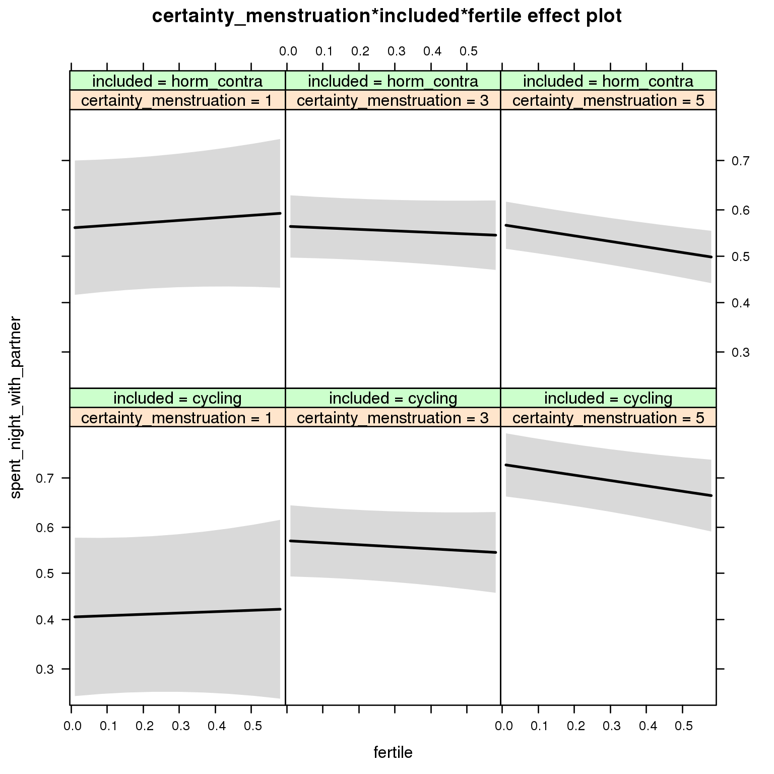
Generalized linear mixed model fit by maximum likelihood (Laplace Approximation) ['glmerMod']
Family: binomial ( probit )
Formula: spent_night_with_partner ~ menstruation + fertile_mean + (1 |
person) + certainty_menstruation + included + fertile + menstruation:included +
certainty_menstruation:included + certainty_menstruation:fertile +
included:fertile + certainty_menstruation:included:fertile
Data: diary
AIC BIC logLik deviance df.resid
26972 27086 -13472 26944 26690
Scaled residuals:
Min 1Q Median 3Q Max
-5.286 -0.599 0.127 0.516 4.914
Random effects:
Groups Name Variance Std.Dev.
person (Intercept) 1.4 1.18
Number of obs: 26704, groups: person, 1054
Fixed effects:
Estimate Std. Error z value Pr(>|z|)
(Intercept) -0.5067 0.2988 -1.70 0.0900 .
menstruationpre -0.0202 0.0477 -0.42 0.6727
menstruationyes -0.0223 0.0454 -0.49 0.6237
fertile_mean 0.3805 0.4961 0.77 0.4431
certainty_menstruation 0.2092 0.0683 3.06 0.0022 **
includedhorm_contra 0.6275 0.3766 1.67 0.0957 .
fertile 0.1654 0.3867 0.43 0.6688
menstruationpre:includedhorm_contra -0.0680 0.0596 -1.14 0.2543
menstruationyes:includedhorm_contra -0.0963 0.0578 -1.67 0.0957 .
certainty_menstruation:includedhorm_contra -0.2048 0.0879 -2.33 0.0197 *
certainty_menstruation:fertile -0.0920 0.0914 -1.01 0.3137
includedhorm_contra:fertile 0.0827 0.4878 0.17 0.8653
certainty_menstruation:includedhorm_contra:fertile -0.0186 0.1133 -0.16 0.8697
---
Signif. codes: 0 '***' 0.001 '**' 0.01 '*' 0.05 '.' 0.1 ' ' 1
convergence code: 0
Model failed to converge with max|grad| = 0.0373847 (tol = 0.001, component 1)
M_m8: Moderation by cycle regularity
model %>%
test_moderator("cycle_regularity", diary)| Df | AIC | BIC | logLik | deviance | Chisq | Chi Df | Pr(>Chisq) | |
|---|---|---|---|---|---|---|---|---|
| with_main | 14 | 26978 | 27093 | -13475 | 26950 | NA | NA | NA |
| with_mod | 18 | 26984 | 27132 | -13474 | 26948 | 2.142 | 4 | 0.7096 |
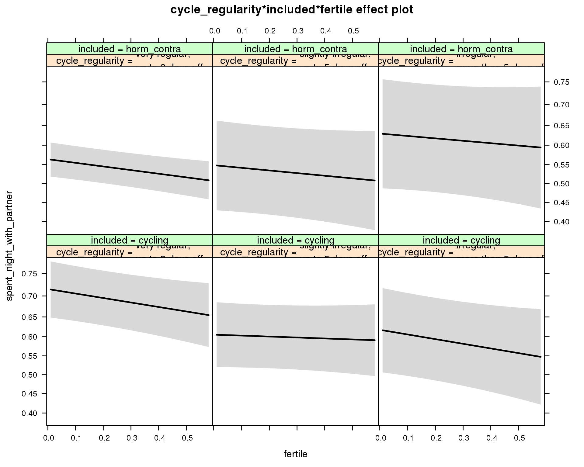
Generalized linear mixed model fit by maximum likelihood (Laplace Approximation) ['glmerMod']
Family: binomial ( probit )
Formula: spent_night_with_partner ~ menstruation + fertile_mean + (1 |
person) + cycle_regularity + included + fertile + menstruation:included +
cycle_regularity:included + cycle_regularity:fertile + included:fertile +
cycle_regularity:included:fertile
Data: diary
AIC BIC logLik deviance df.resid
26984 27132 -13474 26948 26686
Scaled residuals:
Min 1Q Median 3Q Max
-5.518 -0.599 0.126 0.517 4.866
Random effects:
Groups Name Variance Std.Dev.
person (Intercept) 1.4 1.19
Number of obs: 26704, groups: person, 1054
Fixed effects:
Estimate Std. Error z value
(Intercept) 0.4964 0.1272 3.90
menstruationpre -0.0196 0.0478 -0.41
menstruationyes -0.0205 0.0454 -0.45
fertile_mean 0.4677 0.4994 0.94
cycle_regularityslightly irregular,\nup to 5 days off -0.3032 0.1455 -2.08
cycle_regularityirregular,\nmore than 5 days off -0.2711 0.1718 -1.58
includedhorm_contra -0.3807 0.1147 -3.32
fertile -0.2987 0.1371 -2.18
menstruationpre:includedhorm_contra -0.0685 0.0596 -1.15
menstruationyes:includedhorm_contra -0.0966 0.0578 -1.67
cycle_regularityslightly irregular,\nup to 5 days off:includedhorm_contra 0.2633 0.2189 1.20
cycle_regularityirregular,\nmore than 5 days off:includedhorm_contra 0.4417 0.2594 1.70
cycle_regularityslightly irregular,\nup to 5 days off:fertile 0.2347 0.1843 1.27
cycle_regularityirregular,\nmore than 5 days off:fertile -0.0116 0.2289 -0.05
includedhorm_contra:fertile 0.0569 0.1566 0.36
cycle_regularityslightly irregular,\nup to 5 days off:includedhorm_contra:fertile -0.1681 0.2679 -0.63
cycle_regularityirregular,\nmore than 5 days off:includedhorm_contra:fertile 0.0933 0.3336 0.28
Pr(>|z|)
(Intercept) 0.000096 ***
menstruationpre 0.6822
menstruationyes 0.6522
fertile_mean 0.3491
cycle_regularityslightly irregular,\nup to 5 days off 0.0372 *
cycle_regularityirregular,\nmore than 5 days off 0.1146
includedhorm_contra 0.0009 ***
fertile 0.0294 *
menstruationpre:includedhorm_contra 0.2505
menstruationyes:includedhorm_contra 0.0945 .
cycle_regularityslightly irregular,\nup to 5 days off:includedhorm_contra 0.2291
cycle_regularityirregular,\nmore than 5 days off:includedhorm_contra 0.0887 .
cycle_regularityslightly irregular,\nup to 5 days off:fertile 0.2029
cycle_regularityirregular,\nmore than 5 days off:fertile 0.9597
includedhorm_contra:fertile 0.7165
cycle_regularityslightly irregular,\nup to 5 days off:includedhorm_contra:fertile 0.5303
cycle_regularityirregular,\nmore than 5 days off:includedhorm_contra:fertile 0.7798
---
Signif. codes: 0 '***' 0.001 '**' 0.01 '*' 0.05 '.' 0.1 ' ' 1
convergence code: 0
Model failed to converge with max|grad| = 0.0117581 (tol = 0.001, component 1)
M_m9: Moderation by cohabitation status
model %>%
test_moderator("cohabitation", diary)| Df | AIC | BIC | logLik | deviance | Chisq | Chi Df | Pr(>Chisq) | |
|---|---|---|---|---|---|---|---|---|
| with_main | 14 | 26322 | 26436 | -13147 | 26294 | NA | NA | NA |
| with_mod | 18 | 26325 | 26472 | -13145 | 26289 | 4.722 | 4 | 0.317 |
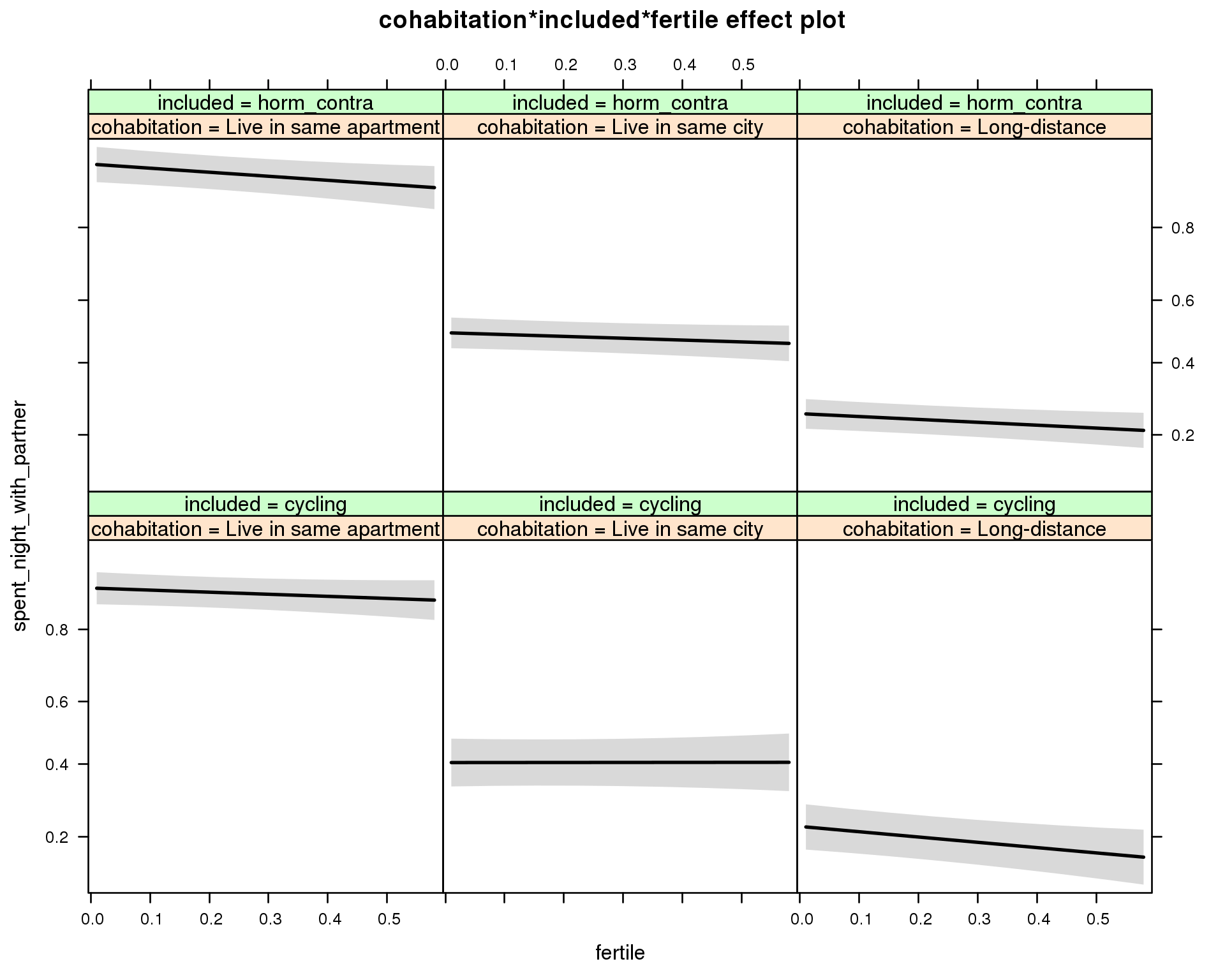
Generalized linear mixed model fit by maximum likelihood (Laplace Approximation) ['glmerMod']
Family: binomial ( probit )
Formula: spent_night_with_partner ~ menstruation + fertile_mean + (1 |
person) + cohabitation + included + fertile + menstruation:included +
cohabitation:included + cohabitation:fertile + included:fertile + cohabitation:included:fertile
Data: diary
AIC BIC logLik deviance df.resid
26325 26472 -13144 26289 26686
Scaled residuals:
Min 1Q Median 3Q Max
-5.617 -0.592 0.136 0.497 4.867
Random effects:
Groups Name Variance Std.Dev.
person (Intercept) 0.643 0.802
Number of obs: 26704, groups: person, 1054
Fixed effects:
Estimate Std. Error z value Pr(>|z|)
(Intercept) 1.11592 0.09521 11.72 <2e-16 ***
menstruationpre -0.01344 0.04788 -0.28 0.779
menstruationyes -0.01226 0.04557 -0.27 0.788
fertile_mean 0.38322 0.38441 1.00 0.319
cohabitationLive in same city -1.41834 0.11925 -11.89 <2e-16 ***
cohabitationLong-distance -1.93751 0.11530 -16.80 <2e-16 ***
includedhorm_contra 0.20855 0.10174 2.05 0.040 *
fertile -0.16895 0.13078 -1.29 0.196
menstruationpre:includedhorm_contra -0.06643 0.05982 -1.11 0.267
menstruationyes:includedhorm_contra -0.09560 0.05801 -1.65 0.099 .
cohabitationLive in same city:includedhorm_contra 0.04836 0.15340 0.32 0.753
cohabitationLong-distance:includedhorm_contra -0.09016 0.14901 -0.61 0.545
cohabitationLive in same city:fertile 0.17224 0.20451 0.84 0.400
cohabitationLong-distance:fertile -0.26130 0.20105 -1.30 0.194
includedhorm_contra:fertile -0.15969 0.19096 -0.84 0.403
cohabitationLive in same city:includedhorm_contra:fertile 0.00691 0.26327 0.03 0.979
cohabitationLong-distance:includedhorm_contra:fertile 0.35542 0.26003 1.37 0.172
---
Signif. codes: 0 '***' 0.001 '**' 0.01 '*' 0.05 '.' 0.1 ' ' 1
convergence code: 0
Model failed to converge with max|grad| = 0.100911 (tol = 0.001, component 1)
M_m10: Moderation by relationship status
model %>%
test_moderator("relationship_status_clean", diary)| Df | AIC | BIC | logLik | deviance | Chisq | Chi Df | Pr(>Chisq) | |
|---|---|---|---|---|---|---|---|---|
| with_main | 14 | 26880 | 26995 | -13426 | 26852 | NA | NA | NA |
| with_mod | 18 | 26886 | 27034 | -13425 | 26850 | 2.329 | 4 | 0.6755 |
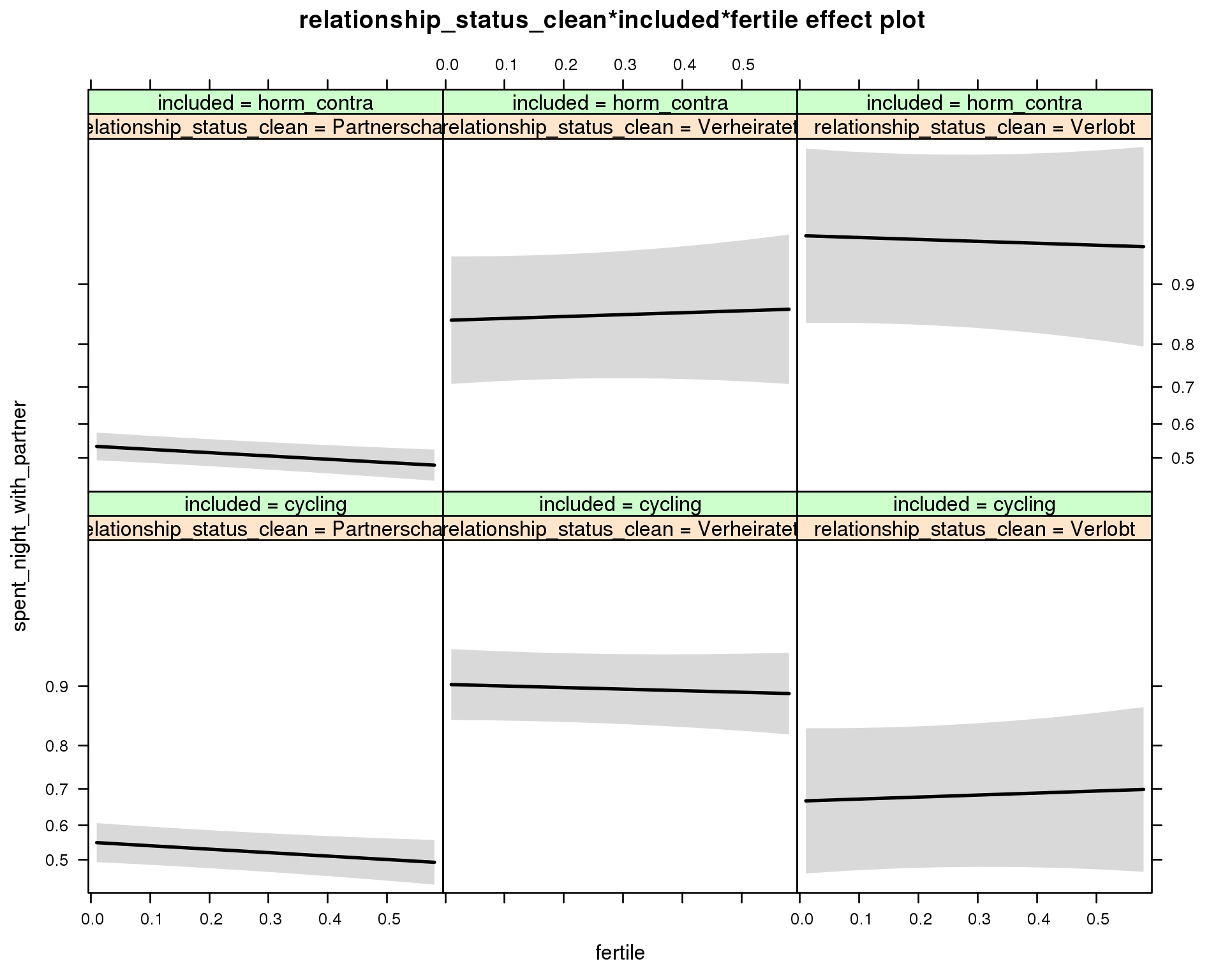
Generalized linear mixed model fit by maximum likelihood (Laplace Approximation) ['glmerMod']
Family: binomial ( probit )
Formula: spent_night_with_partner ~ menstruation + fertile_mean + (1 |
person) + relationship_status_clean + included + fertile +
menstruation:included + relationship_status_clean:included +
relationship_status_clean:fertile + included:fertile + relationship_status_clean:included:fertile
Data: diary
AIC BIC logLik deviance df.resid
26886 27034 -13425 26850 26686
Scaled residuals:
Min 1Q Median 3Q Max
-5.620 -0.598 0.126 0.512 4.841
Random effects:
Groups Name Variance Std.Dev.
person (Intercept) 1.28 1.13
Number of obs: 26704, groups: person, 1054
Fixed effects:
Estimate Std. Error z value Pr(>|z|)
(Intercept) 0.0542 0.1116 0.49 0.6275
menstruationpre -0.0164 0.0483 -0.34 0.7350
menstruationyes -0.0170 0.0460 -0.37 0.7116
fertile_mean 0.4617 0.4874 0.95 0.3435
relationship_status_cleanVerheiratet 1.1655 0.1523 7.65 2e-14 ***
relationship_status_cleanVerlobt 0.3043 0.2839 1.07 0.2837
includedhorm_contra -0.0103 0.0939 -0.11 0.9128
fertile -0.2548 0.1084 -2.35 0.0187 *
menstruationpre:includedhorm_contra -0.0730 0.0602 -1.21 0.2253
menstruationyes:includedhorm_contra -0.1009 0.0584 -1.73 0.0838 .
relationship_status_cleanVerheiratet:includedhorm_contra -0.2371 0.2897 -0.82 0.4131
relationship_status_cleanVerlobt:includedhorm_contra 1.2496 0.4378 2.85 0.0043 **
relationship_status_cleanVerheiratet:fertile 0.1391 0.2210 0.63 0.5291
relationship_status_cleanVerlobt:fertile 0.4028 0.4021 1.00 0.3165
includedhorm_contra:fertile 0.0118 0.1299 0.09 0.9275
relationship_status_cleanVerheiratet:includedhorm_contra:fertile 0.2445 0.4370 0.56 0.5757
relationship_status_cleanVerlobt:includedhorm_contra:fertile -0.3009 0.6234 -0.48 0.6294
---
Signif. codes: 0 '***' 0.001 '**' 0.01 '*' 0.05 '.' 0.1 ' ' 1
convergence code: 0
Model failed to converge with max|grad| = 0.0976386 (tol = 0.001, component 1)
Male mate retention
model_summaries$partner_mate_retentionModel summary
Model summary
model %>%
print_summary()Linear mixed model fit by REML
t-tests use Satterthwaite approximations to degrees of freedom ['lmerMod']
Formula: partner_mate_retention ~ included * (menstruation + fertile) + fertile_mean + (1 | person)
Data: diary
REML criterion at convergence: 66936
Scaled residuals:
Min 1Q Median 3Q Max
-4.691 -0.609 0.010 0.613 4.870
Random effects:
Groups Name Variance Std.Dev.
person (Intercept) 0.540 0.735
Residual 0.642 0.801
Number of obs: 26680, groups: person, 1054
Fixed effects:
Estimate Std. Error df t value Pr(>|t|)
(Intercept) 2.8108 0.0627 1342.0000 44.85 <2e-16 ***
includedhorm_contra 0.0882 0.0514 1293.0000 1.72 0.0863 .
menstruationpre -0.0317 0.0245 25932.0000 -1.29 0.1956
menstruationyes -0.0600 0.0231 26031.0000 -2.60 0.0093 **
fertile 0.0381 0.0494 25923.0000 0.77 0.4405
fertile_mean -0.1062 0.2863 1457.0000 -0.37 0.7107
includedhorm_contra:menstruationpre 0.0207 0.0314 25928.0000 0.66 0.5107
includedhorm_contra:menstruationyes 0.0130 0.0302 26011.0000 0.43 0.6671
includedhorm_contra:fertile -0.0984 0.0626 26036.0000 -1.57 0.1159
---
Signif. codes: 0 '***' 0.001 '**' 0.01 '*' 0.05 '.' 0.1 ' ' 1
Correlation of Fixed Effects:
(Intr) incld_ mnstrtnp mnstrtny fertil frtl_m inclddhrm_cntr:mnstrtnp
inclddhrm_c -0.474
menstrutnpr -0.149 0.190
menstrutnys -0.146 0.183 0.398
fertile -0.144 0.235 0.467 0.385
fertile_men -0.772 -0.025 -0.008 -0.005 -0.062
inclddhrm_cntr:mnstrtnp 0.124 -0.238 -0.779 -0.310 -0.363 -0.003
inclddhrm_cntr:mnstrtny 0.117 -0.225 -0.303 -0.763 -0.293 -0.003 0.383
inclddhrm_cntr:f 0.144 -0.297 -0.368 -0.303 -0.787 0.010 0.467
inclddhrm_cntr:mnstrtny
inclddhrm_c
menstrutnpr
menstrutnys
fertile
fertile_men
inclddhrm_cntr:mnstrtnp
inclddhrm_cntr:mnstrtny
inclddhrm_cntr:f 0.381
Effect size standardised by residual variance (\(\frac{b}{ SD_{residual} }\)): 0.05 [-0.07;0.17].
Marginal effect plots
model %>%
plot_all_effects()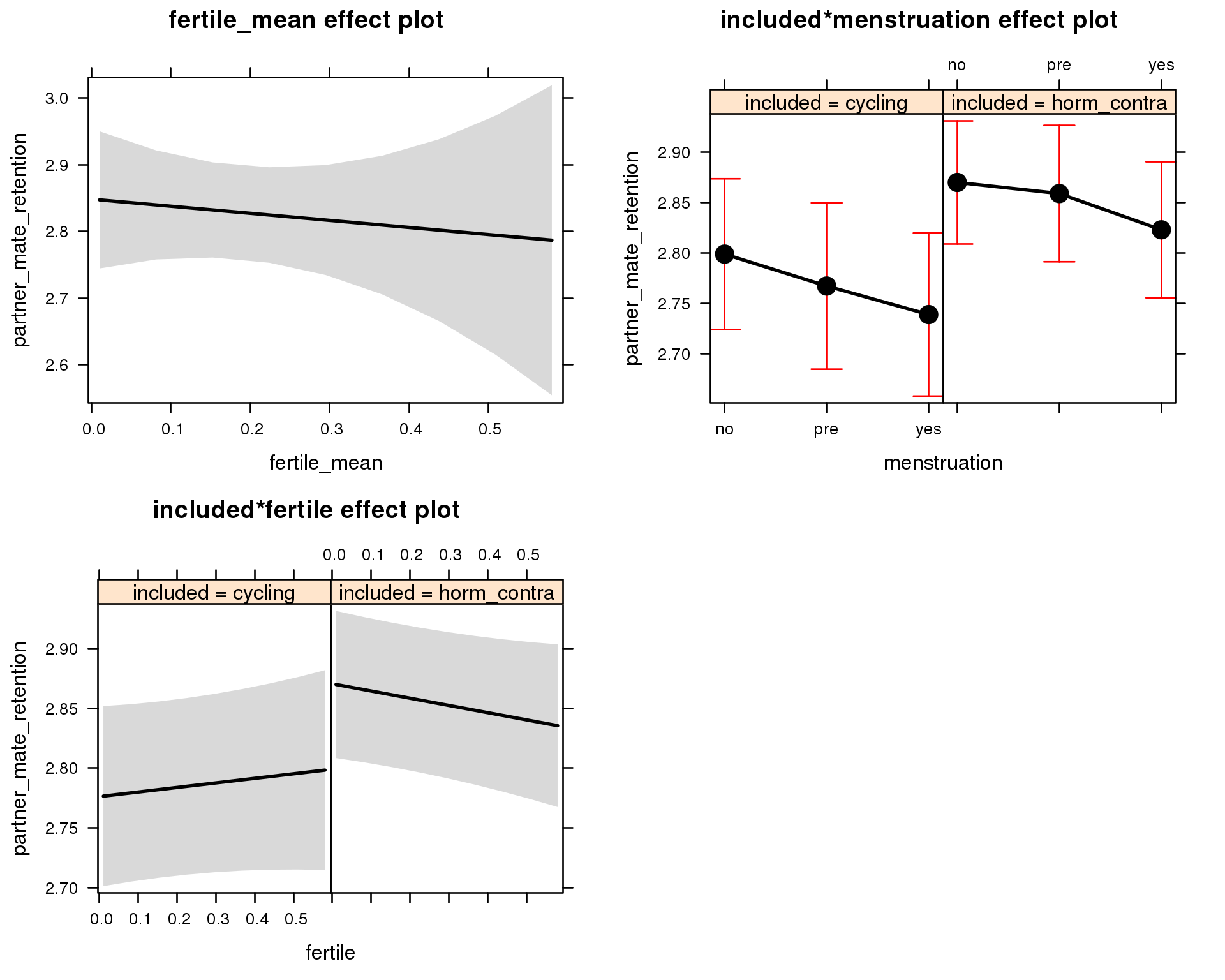
Outcome distribution
model %>%
plot_outcome(diary) + xlab(outcome_label)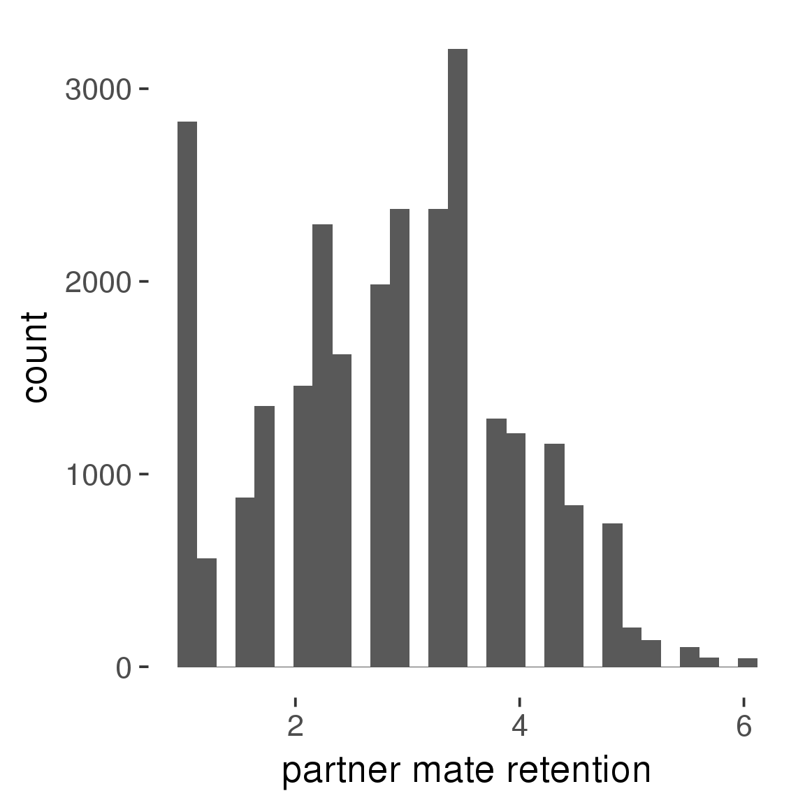
Diagnostics
model %>%
print_diagnostics()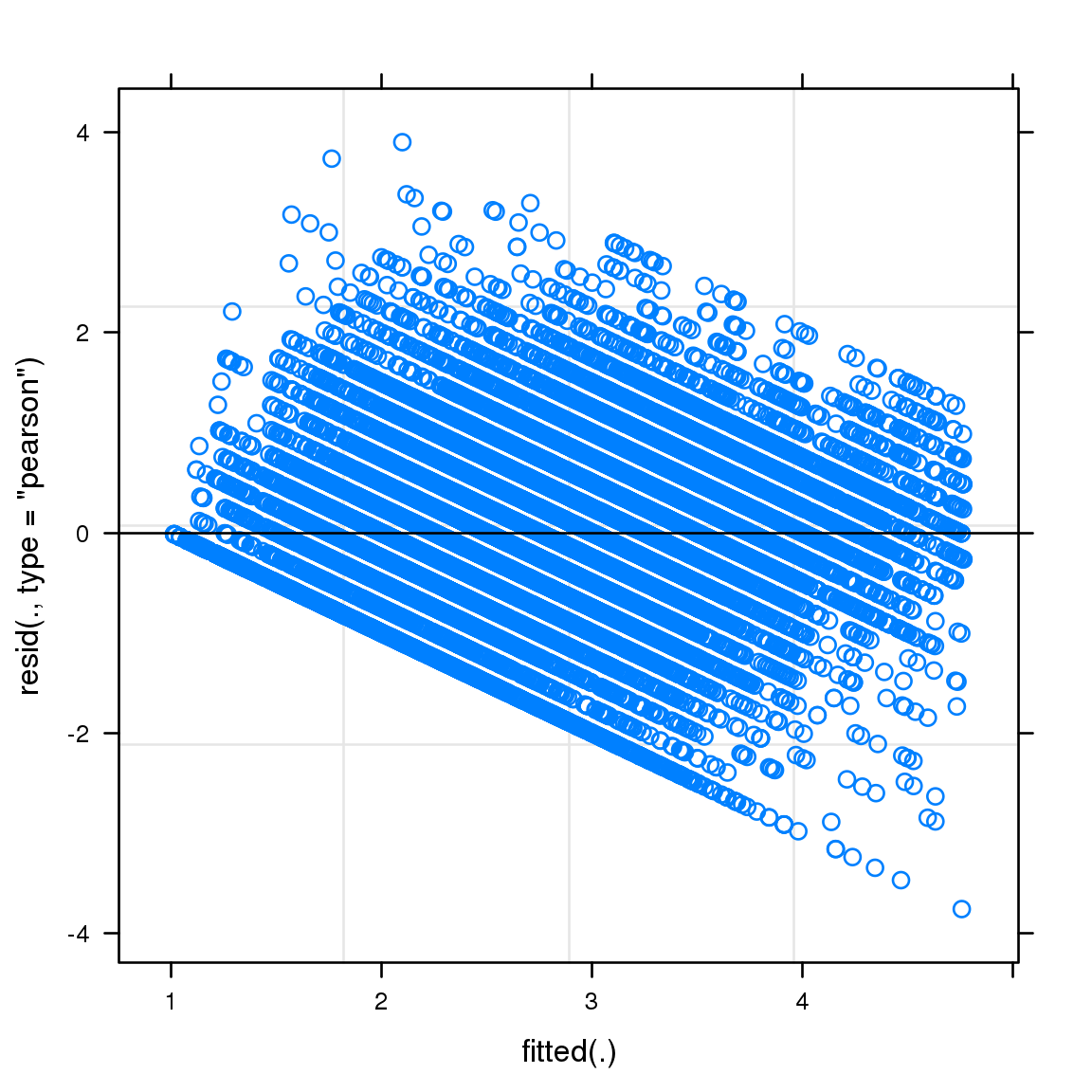
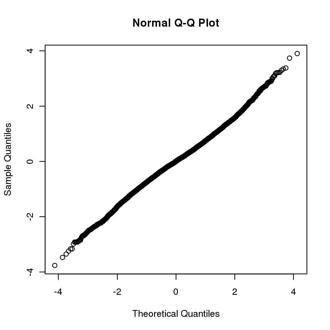
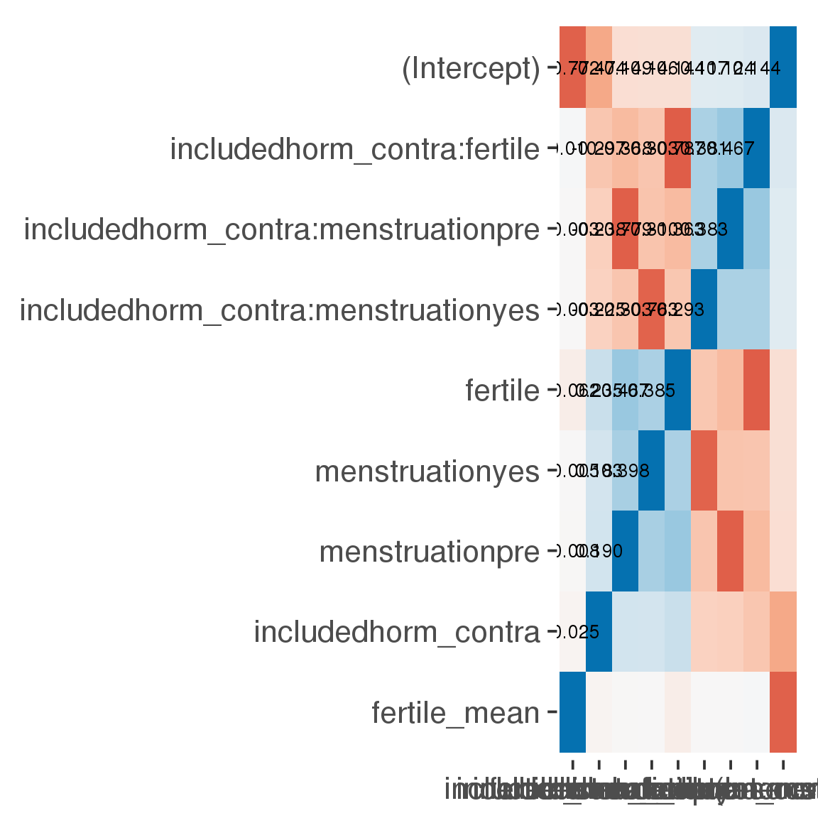
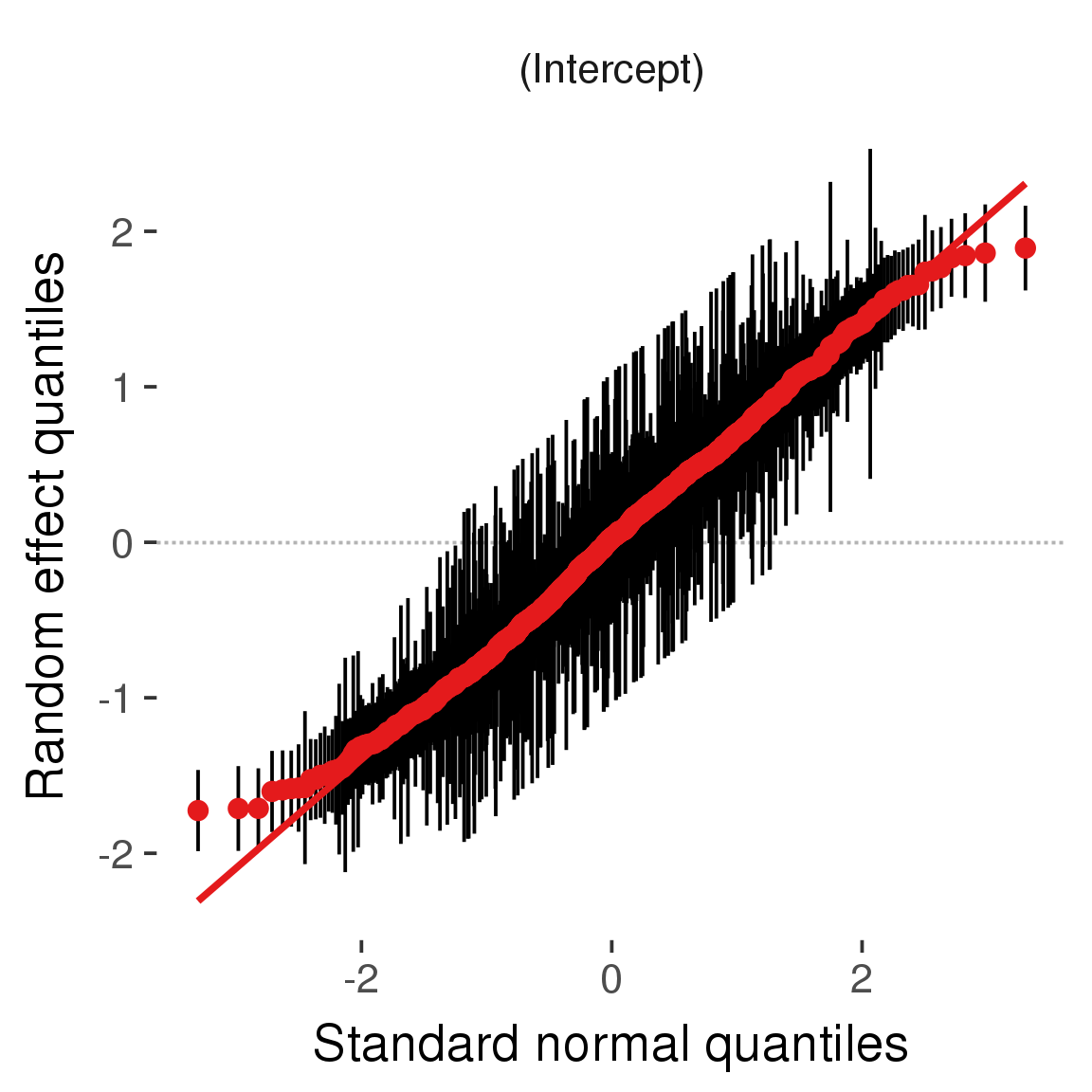
Curves
Here, we continuously plot the outcome over the course of the cycle. Because cycle lengths vary, we subset the data to cycles in a certain range. If the red curve traces the pink curve, our predictor accurately maps the relationship between fertile window probability and the outcome.
Cycle lengths from 21 to 36
Backward-counted
model %>%
plot_curve(diary %>% filter(minimum_cycle_length_diary <= 36, minimum_cycle_length_diary > 20) %>% mutate(fertile=prc_stirn_b))outcome = names(model@frame)[1]
outcome_label = recode(str_replace_all(str_replace_all(str_replace_all(outcome, "_", " "), " pair", "-pair"), " 1", ""),
"desirability 1" = "self-perceived desirability",
"NARQ admiration" = "narcissistic admiration",
"NARQ rivalry" = "narcissistic rivalry",
"extra-pair" = "extra-pair desire & behaviour",
"had sexual intercourse" = "sexual intercourse")
library(ggplot2)
# form a subset and run the model without the hormonal contraception and the fertility predictors
tmp = diary %>%
filter(!is.na(fertile), !is.na(included),
RCD > -1 * minimum_cycle_length_diary, RCD > -40)
new_form = update.formula(formula(model), new = . ~ . - fertile * included)
tmp$residuals = residuals(update(model, new_form, data = tmp , na.action = na.exclude))
tmp = tmp %>%
filter(!is.na(RCD), !is.na(residuals))
rcd_min = min(tmp$RCD)
tmp$real = FALSE
tmp_before = tmp
tmp_before$RCD = tmp_before$RCD + min(tmp$RCD) - 1
tmp_after = tmp
tmp_after$RCD = tmp_after$RCD - min(tmp$RCD) + 1
tmp$real = TRUE
tmp = bind_rows(tmp_before %>% filter(RCD > rcd_min - 11), tmp, tmp_after %>% filter(RCD < 11))GAM smooth on residuals
Here, we partialled out menstruation and individual random effects, then superimposed estimated probability of being in the fertile window scaled to the range of the estimated means. To address the periodicity of the cycle, we prepended and appended ten days of the timeseries to the end and the beginning of the timeseries. We then estimated the GAM and cut off the appended subsets before plotting.
tryCatch({
trend_plot = ggplot(tmp,aes(x = RCD, y = residuals, colour = included)) +
stat_smooth(geom = 'smooth',size = 0.8, fill = "#9ECAE1", method = 'gam', formula = y ~ s(x))
}, error = function(e){cat_message(e, "danger")})
tryCatch({
trend_data = ggplot_build(trend_plot)$data[[1]]
}, error = function(e){cat_message(e, "danger")})
trend_data$RCD = round(trend_data$x)
trend_data = left_join(trend_data, tmp %>% select(real, RCD,fertile) %>% unique(), by = "RCD")
trend_data %>%
filter(real == TRUE) %>%
mutate(superimposed = ( ( (fertile - 0.01)/0.58) * (max(y)-min(y) ) ) + min(y) ) ->
trend_data
ggplot(trend_data) +
geom_ribbon(aes(x = x, ymin = ymin, ymax = ymax, fill = factor(group)), alpha = 0.2) +
geom_line(aes(x = x, y = y, colour = factor(group)), size = 0.8, stat = "identity") +
scale_x_continuous(caption_x) +
geom_line(aes(x = x, y = superimposed), color = "#a83fbf", size = 1, linetype = 'dashed') +
annotate("text",x = mean(trend_data$x), y = max(trend_data$superimposed,na.rm=T) + 0.1, label = 'superimposed fertility peak', color = "#a83fbf") +
scale_y_continuous(outcome_label) +
ggtitle("GAM smooth, residuals") +
scale_color_manual("Contraception status",values = c("2"="black","1"= "red"), labels = c("2"="hormonally\ncontracepting","1"="cycling"), guide = F) +
scale_fill_manual("Contraception status",values = c("2"="black","1"= "red"), labels = c("2"="hormonally\ncontracepting","1"="cycling"), guide = F)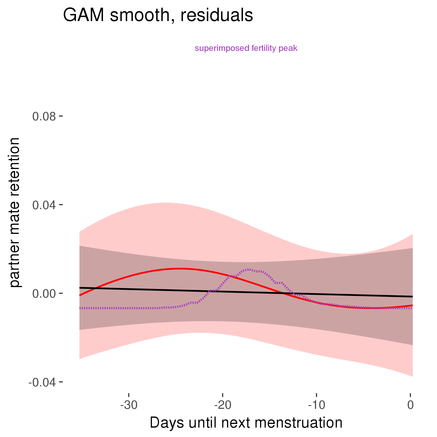
GAM smooth on raw data
As before, but without partialling anything out.
tryCatch({
trend_plot = ggplot(tmp,aes_string(x = "RCD", y = outcome, colour = "included")) +
stat_smooth(geom = 'smooth',size = 0.8, fill = "#9ECAE1", method = 'gam', formula = y ~ s(x))
}, error = function(e){cat_message(e, "danger")})
tryCatch({
trend_data = ggplot_build(trend_plot)$data[[1]]
}, error = function(e){cat_message(e, "danger")})
trend_data$RCD = round(trend_data$x)
trend_data = left_join(trend_data, tmp %>% select(real, RCD,fertile) %>% unique(), by = "RCD")
trend_data %>%
filter(real == TRUE) %>%
mutate(superimposed = ( ( (fertile - 0.01)/0.58) * (max(y)-min(y) ) ) + min(y) ) ->
trend_data
plot1b = ggplot(trend_data) +
geom_ribbon(aes(x = x, ymin = ymin, ymax = ymax, fill = factor(group)), alpha = 0.2) +
geom_line(aes(x = x, y = y, colour = factor(group)), size = 0.8, stat = "identity") +
scale_x_continuous(caption_x) +
geom_line(aes(x = x, y = superimposed), color = "#a83fbf", size = 1, linetype = 'dashed') +
annotate("text",x = mean(trend_data$x), y = max(trend_data$superimposed,na.rm=T) + 0.1, label = 'superimposed fertility peak', color = "#a83fbf") +
scale_y_continuous(outcome_label) +
ggtitle("GAM smooth, raw data") +
scale_color_manual("Contraception status",values = c("2"="black","1"= "red"), labels = c("2"="hormonally\ncontracepting","1"="cycling"), guide = F) +
scale_fill_manual("Contraception status",values = c("2"="black","1"= "red"), labels = c("2"="hormonally\ncontracepting","1"="cycling"), guide = F)
suppressWarnings(print(plot1b))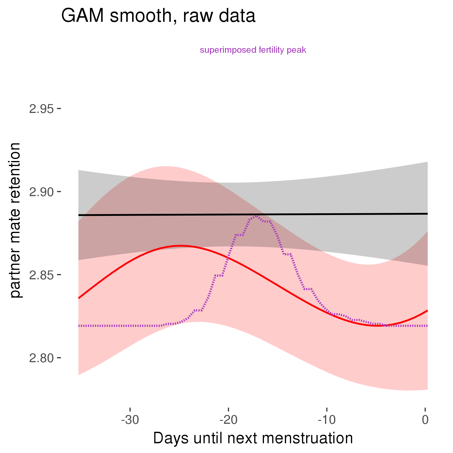
Means and standard errors over raw data
Nothing partialled out, just straight means with bootstrapped confidence intervals.
tryCatch({
trend_plot = ggplot(tmp,aes_string(x = "RCD", y = outcome, colour = "included")) +
geom_pointrange(size = 0.8, stat = 'summary', fun.data = "mean_cl_boot")
}, error = function(e){cat_message(e, "danger")})
tryCatch({
trend_data = ggplot_build(trend_plot)$data[[1]]
}, error = function(e){cat_message(e, "danger")})
trend_data$RCD = round(trend_data$x)
trend_data = left_join(trend_data, tmp %>% select(real, RCD,fertile) %>% unique(), by = "RCD")
trend_data %>%
filter(real == TRUE) %>%
mutate(superimposed = ( ( (fertile - 0.01)/0.58) * (max(y)-min(y) ) ) + min(y) ) ->
trend_data
plot3 = ggplot(trend_data) +
geom_pointrange(aes(x = x, y = y, ymin = ymin,ymax = ymax, colour = factor(group)), size = 0.8, stat = "identity", alpha = 0.6, position = position_dodge(width = .5)) +
scale_x_continuous("Days until next menstruation") +
geom_line(aes(x= x, y = superimposed), color = "#a83fbf", size = 1, linetype = 'dashed') +
annotate("text",x = mean(trend_data$x), y = max(trend_data$superimposed,na.rm=T) + 0.1, label = 'superimposed fertility peak', color = "#a83fbf") +
scale_y_continuous(outcome_label) +
ggtitle("Means with standard errors, raw data") +
scale_color_manual("Contraception status",values = c("2"="black","1"= "red"), labels = c("2"="hormonally\ncontracepting","1"="cycling"), guide = F) +
scale_fill_manual("Contraception status",values = c("2"="black","1"= "red"), labels = c("2"="hormonally\ncontracepting","1"="cycling"), guide = F)
suppressWarnings(print(plot3))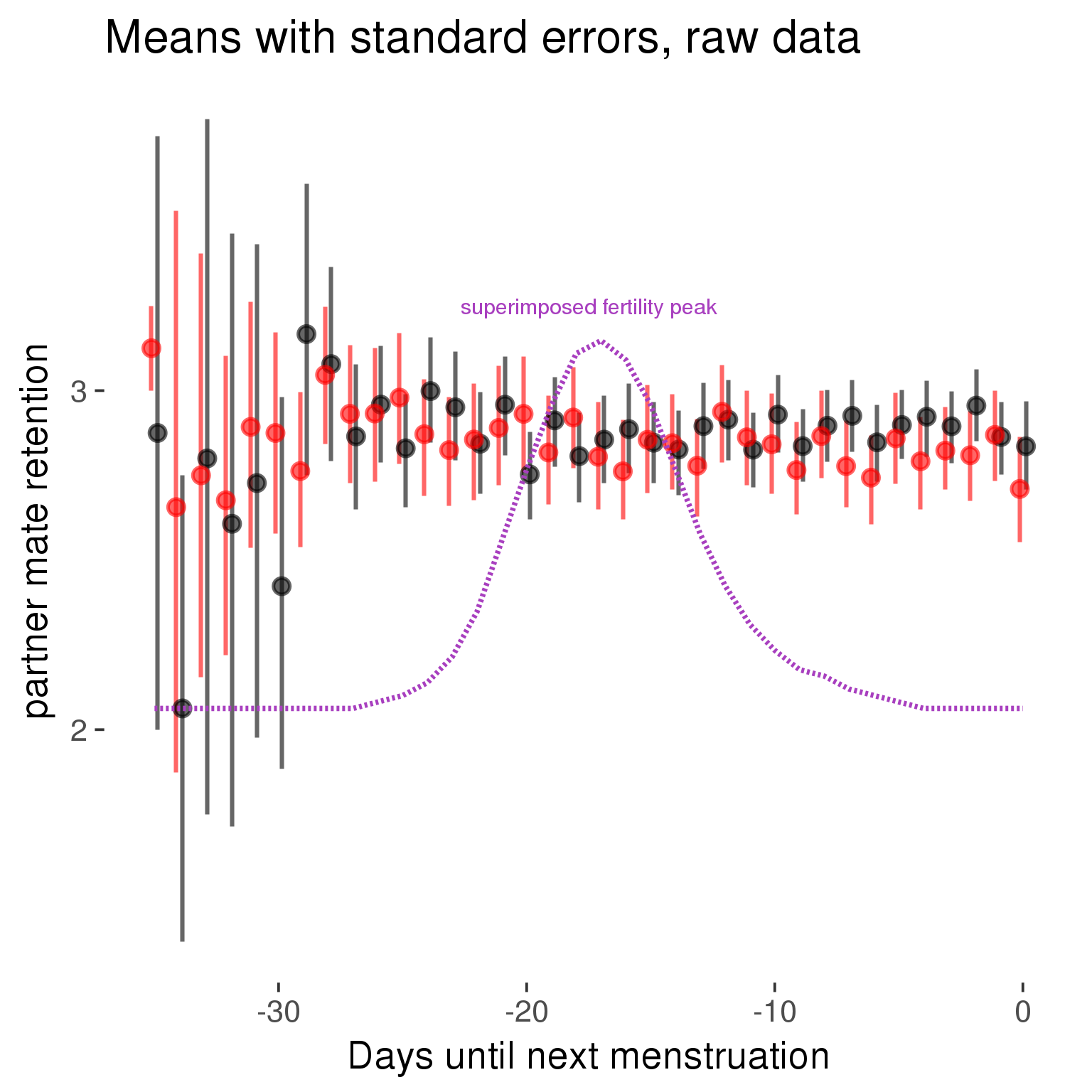
Forward-counted
model %>%
plot_curve(diary %>% filter(minimum_cycle_length_diary <= 36, minimum_cycle_length_diary > 20) %>% mutate(RCD = FCD, fertile = prc_stirn_b_forward_counted), caption_x = "Days since last menstruation")outcome = names(model@frame)[1]
outcome_label = recode(str_replace_all(str_replace_all(str_replace_all(outcome, "_", " "), " pair", "-pair"), " 1", ""),
"desirability 1" = "self-perceived desirability",
"NARQ admiration" = "narcissistic admiration",
"NARQ rivalry" = "narcissistic rivalry",
"extra-pair" = "extra-pair desire & behaviour",
"had sexual intercourse" = "sexual intercourse")
library(ggplot2)
# form a subset and run the model without the hormonal contraception and the fertility predictors
tmp = diary %>%
filter(!is.na(fertile), !is.na(included),
RCD > -1 * minimum_cycle_length_diary, RCD > -40)
new_form = update.formula(formula(model), new = . ~ . - fertile * included)
tmp$residuals = residuals(update(model, new_form, data = tmp , na.action = na.exclude))
tmp = tmp %>%
filter(!is.na(RCD), !is.na(residuals))
rcd_min = min(tmp$RCD)
tmp$real = FALSE
tmp_before = tmp
tmp_before$RCD = tmp_before$RCD + min(tmp$RCD) - 1
tmp_after = tmp
tmp_after$RCD = tmp_after$RCD - min(tmp$RCD) + 1
tmp$real = TRUE
tmp = bind_rows(tmp_before %>% filter(RCD > rcd_min - 11), tmp, tmp_after %>% filter(RCD < 11))GAM smooth on residuals
Here, we partialled out menstruation and individual random effects, then superimposed estimated probability of being in the fertile window scaled to the range of the estimated means. To address the periodicity of the cycle, we prepended and appended ten days of the timeseries to the end and the beginning of the timeseries. We then estimated the GAM and cut off the appended subsets before plotting.
tryCatch({
trend_plot = ggplot(tmp,aes(x = RCD, y = residuals, colour = included)) +
stat_smooth(geom = 'smooth',size = 0.8, fill = "#9ECAE1", method = 'gam', formula = y ~ s(x))
}, error = function(e){cat_message(e, "danger")})
tryCatch({
trend_data = ggplot_build(trend_plot)$data[[1]]
}, error = function(e){cat_message(e, "danger")})
trend_data$RCD = round(trend_data$x)
trend_data = left_join(trend_data, tmp %>% select(real, RCD,fertile) %>% unique(), by = "RCD")
trend_data %>%
filter(real == TRUE) %>%
mutate(superimposed = ( ( (fertile - 0.01)/0.58) * (max(y)-min(y) ) ) + min(y) ) ->
trend_data
ggplot(trend_data) +
geom_ribbon(aes(x = x, ymin = ymin, ymax = ymax, fill = factor(group)), alpha = 0.2) +
geom_line(aes(x = x, y = y, colour = factor(group)), size = 0.8, stat = "identity") +
scale_x_continuous(caption_x) +
geom_line(aes(x = x, y = superimposed), color = "#a83fbf", size = 1, linetype = 'dashed') +
annotate("text",x = mean(trend_data$x), y = max(trend_data$superimposed,na.rm=T) + 0.1, label = 'superimposed fertility peak', color = "#a83fbf") +
scale_y_continuous(outcome_label) +
ggtitle("GAM smooth, residuals") +
scale_color_manual("Contraception status",values = c("2"="black","1"= "red"), labels = c("2"="hormonally\ncontracepting","1"="cycling"), guide = F) +
scale_fill_manual("Contraception status",values = c("2"="black","1"= "red"), labels = c("2"="hormonally\ncontracepting","1"="cycling"), guide = F)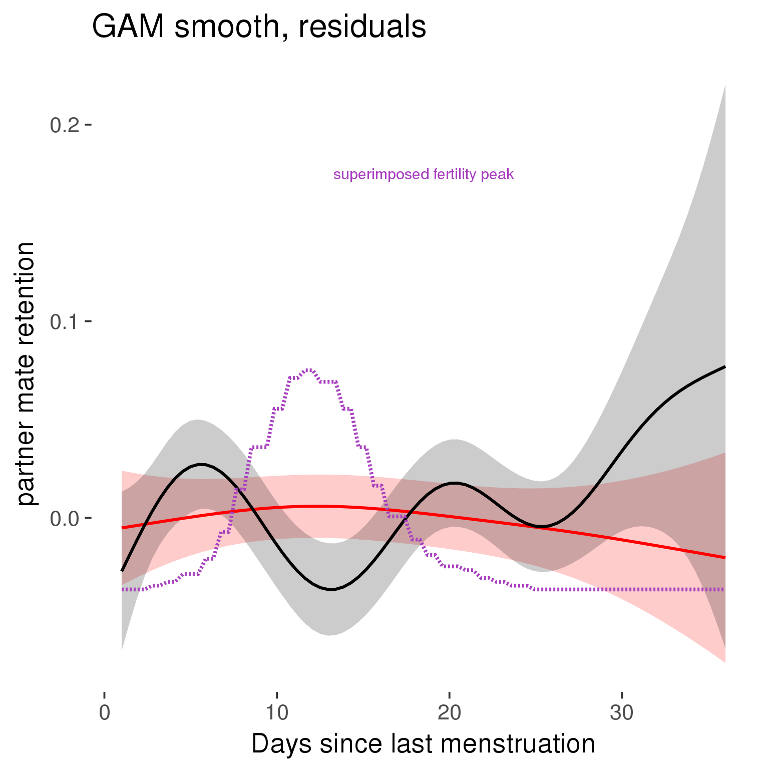
GAM smooth on raw data
As before, but without partialling anything out.
tryCatch({
trend_plot = ggplot(tmp,aes_string(x = "RCD", y = outcome, colour = "included")) +
stat_smooth(geom = 'smooth',size = 0.8, fill = "#9ECAE1", method = 'gam', formula = y ~ s(x))
}, error = function(e){cat_message(e, "danger")})
tryCatch({
trend_data = ggplot_build(trend_plot)$data[[1]]
}, error = function(e){cat_message(e, "danger")})
trend_data$RCD = round(trend_data$x)
trend_data = left_join(trend_data, tmp %>% select(real, RCD,fertile) %>% unique(), by = "RCD")
trend_data %>%
filter(real == TRUE) %>%
mutate(superimposed = ( ( (fertile - 0.01)/0.58) * (max(y)-min(y) ) ) + min(y) ) ->
trend_data
plot1b = ggplot(trend_data) +
geom_ribbon(aes(x = x, ymin = ymin, ymax = ymax, fill = factor(group)), alpha = 0.2) +
geom_line(aes(x = x, y = y, colour = factor(group)), size = 0.8, stat = "identity") +
scale_x_continuous(caption_x) +
geom_line(aes(x = x, y = superimposed), color = "#a83fbf", size = 1, linetype = 'dashed') +
annotate("text",x = mean(trend_data$x), y = max(trend_data$superimposed,na.rm=T) + 0.1, label = 'superimposed fertility peak', color = "#a83fbf") +
scale_y_continuous(outcome_label) +
ggtitle("GAM smooth, raw data") +
scale_color_manual("Contraception status",values = c("2"="black","1"= "red"), labels = c("2"="hormonally\ncontracepting","1"="cycling"), guide = F) +
scale_fill_manual("Contraception status",values = c("2"="black","1"= "red"), labels = c("2"="hormonally\ncontracepting","1"="cycling"), guide = F)
suppressWarnings(print(plot1b))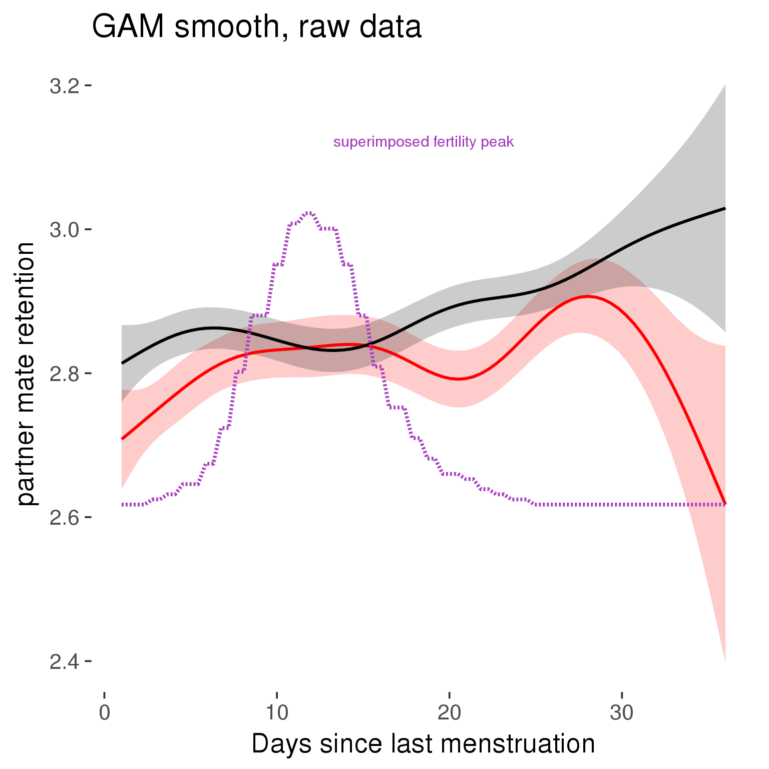
Means and standard errors over raw data
Nothing partialled out, just straight means with bootstrapped confidence intervals.
tryCatch({
trend_plot = ggplot(tmp,aes_string(x = "RCD", y = outcome, colour = "included")) +
geom_pointrange(size = 0.8, stat = 'summary', fun.data = "mean_cl_boot")
}, error = function(e){cat_message(e, "danger")})
tryCatch({
trend_data = ggplot_build(trend_plot)$data[[1]]
}, error = function(e){cat_message(e, "danger")})
trend_data$RCD = round(trend_data$x)
trend_data = left_join(trend_data, tmp %>% select(real, RCD,fertile) %>% unique(), by = "RCD")
trend_data %>%
filter(real == TRUE) %>%
mutate(superimposed = ( ( (fertile - 0.01)/0.58) * (max(y)-min(y) ) ) + min(y) ) ->
trend_data
plot3 = ggplot(trend_data) +
geom_pointrange(aes(x = x, y = y, ymin = ymin,ymax = ymax, colour = factor(group)), size = 0.8, stat = "identity", alpha = 0.6, position = position_dodge(width = .5)) +
scale_x_continuous("Days until next menstruation") +
geom_line(aes(x= x, y = superimposed), color = "#a83fbf", size = 1, linetype = 'dashed') +
annotate("text",x = mean(trend_data$x), y = max(trend_data$superimposed,na.rm=T) + 0.1, label = 'superimposed fertility peak', color = "#a83fbf") +
scale_y_continuous(outcome_label) +
ggtitle("Means with standard errors, raw data") +
scale_color_manual("Contraception status",values = c("2"="black","1"= "red"), labels = c("2"="hormonally\ncontracepting","1"="cycling"), guide = F) +
scale_fill_manual("Contraception status",values = c("2"="black","1"= "red"), labels = c("2"="hormonally\ncontracepting","1"="cycling"), guide = F)
suppressWarnings(print(plot3))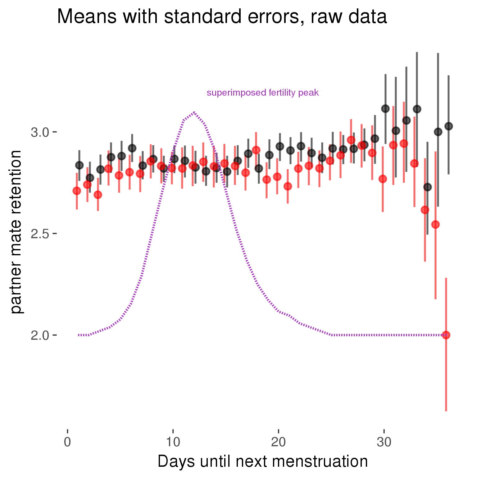
Cycle lengths from 27 to 30
Backward-counted
model %>%
plot_curve(diary %>% filter(minimum_cycle_length_diary <= 30, minimum_cycle_length_diary >= 27) %>% mutate(fertile=prc_stirn_b))outcome = names(model@frame)[1]
outcome_label = recode(str_replace_all(str_replace_all(str_replace_all(outcome, "_", " "), " pair", "-pair"), " 1", ""),
"desirability 1" = "self-perceived desirability",
"NARQ admiration" = "narcissistic admiration",
"NARQ rivalry" = "narcissistic rivalry",
"extra-pair" = "extra-pair desire & behaviour",
"had sexual intercourse" = "sexual intercourse")
library(ggplot2)
# form a subset and run the model without the hormonal contraception and the fertility predictors
tmp = diary %>%
filter(!is.na(fertile), !is.na(included),
RCD > -1 * minimum_cycle_length_diary, RCD > -40)
new_form = update.formula(formula(model), new = . ~ . - fertile * included)
tmp$residuals = residuals(update(model, new_form, data = tmp , na.action = na.exclude))
tmp = tmp %>%
filter(!is.na(RCD), !is.na(residuals))
rcd_min = min(tmp$RCD)
tmp$real = FALSE
tmp_before = tmp
tmp_before$RCD = tmp_before$RCD + min(tmp$RCD) - 1
tmp_after = tmp
tmp_after$RCD = tmp_after$RCD - min(tmp$RCD) + 1
tmp$real = TRUE
tmp = bind_rows(tmp_before %>% filter(RCD > rcd_min - 11), tmp, tmp_after %>% filter(RCD < 11))GAM smooth on residuals
Here, we partialled out menstruation and individual random effects, then superimposed estimated probability of being in the fertile window scaled to the range of the estimated means. To address the periodicity of the cycle, we prepended and appended ten days of the timeseries to the end and the beginning of the timeseries. We then estimated the GAM and cut off the appended subsets before plotting.
tryCatch({
trend_plot = ggplot(tmp,aes(x = RCD, y = residuals, colour = included)) +
stat_smooth(geom = 'smooth',size = 0.8, fill = "#9ECAE1", method = 'gam', formula = y ~ s(x))
}, error = function(e){cat_message(e, "danger")})
tryCatch({
trend_data = ggplot_build(trend_plot)$data[[1]]
}, error = function(e){cat_message(e, "danger")})
trend_data$RCD = round(trend_data$x)
trend_data = left_join(trend_data, tmp %>% select(real, RCD,fertile) %>% unique(), by = "RCD")
trend_data %>%
filter(real == TRUE) %>%
mutate(superimposed = ( ( (fertile - 0.01)/0.58) * (max(y)-min(y) ) ) + min(y) ) ->
trend_data
ggplot(trend_data) +
geom_ribbon(aes(x = x, ymin = ymin, ymax = ymax, fill = factor(group)), alpha = 0.2) +
geom_line(aes(x = x, y = y, colour = factor(group)), size = 0.8, stat = "identity") +
scale_x_continuous(caption_x) +
geom_line(aes(x = x, y = superimposed), color = "#a83fbf", size = 1, linetype = 'dashed') +
annotate("text",x = mean(trend_data$x), y = max(trend_data$superimposed,na.rm=T) + 0.1, label = 'superimposed fertility peak', color = "#a83fbf") +
scale_y_continuous(outcome_label) +
ggtitle("GAM smooth, residuals") +
scale_color_manual("Contraception status",values = c("2"="black","1"= "red"), labels = c("2"="hormonally\ncontracepting","1"="cycling"), guide = F) +
scale_fill_manual("Contraception status",values = c("2"="black","1"= "red"), labels = c("2"="hormonally\ncontracepting","1"="cycling"), guide = F)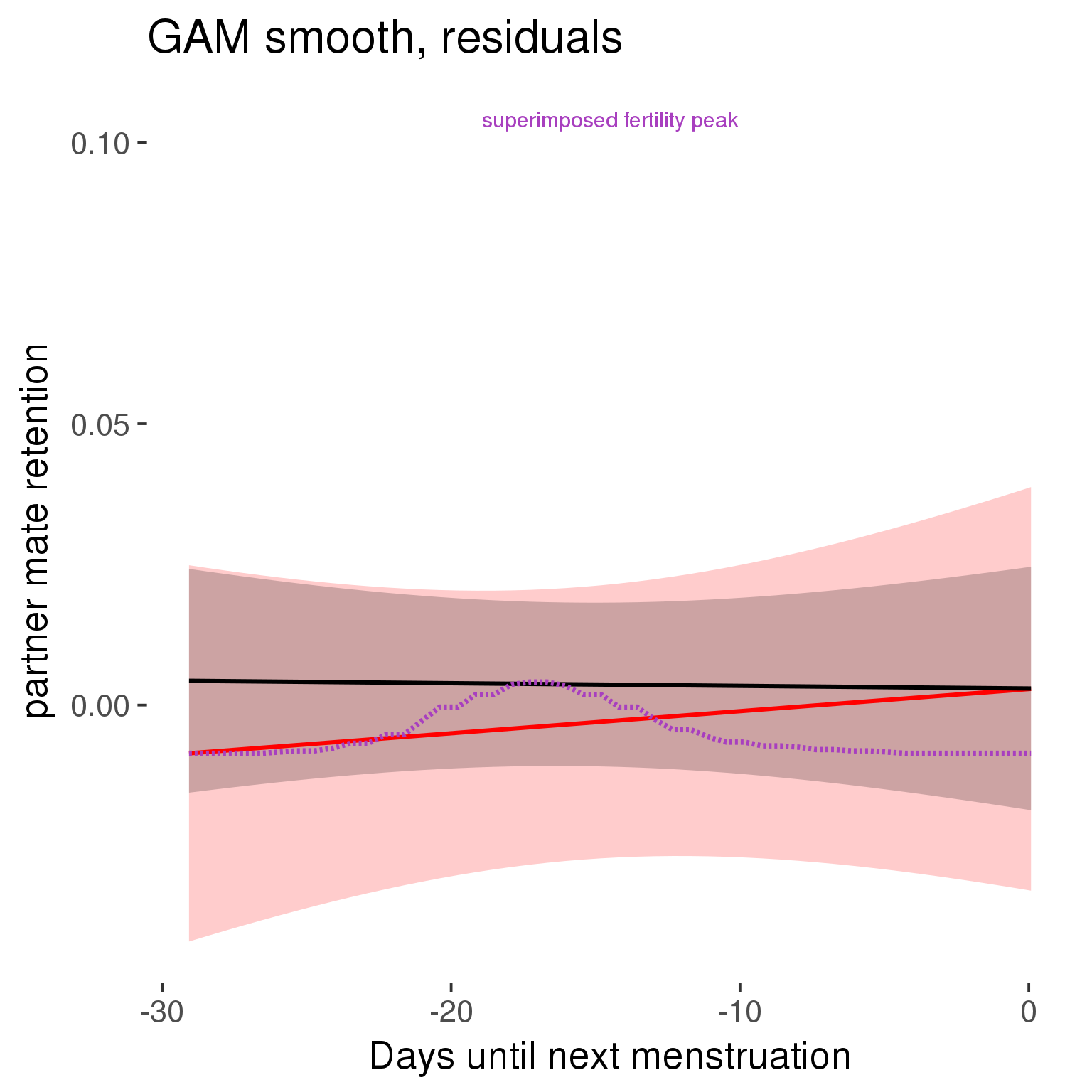
GAM smooth on raw data
As before, but without partialling anything out.
tryCatch({
trend_plot = ggplot(tmp,aes_string(x = "RCD", y = outcome, colour = "included")) +
stat_smooth(geom = 'smooth',size = 0.8, fill = "#9ECAE1", method = 'gam', formula = y ~ s(x))
}, error = function(e){cat_message(e, "danger")})
tryCatch({
trend_data = ggplot_build(trend_plot)$data[[1]]
}, error = function(e){cat_message(e, "danger")})
trend_data$RCD = round(trend_data$x)
trend_data = left_join(trend_data, tmp %>% select(real, RCD,fertile) %>% unique(), by = "RCD")
trend_data %>%
filter(real == TRUE) %>%
mutate(superimposed = ( ( (fertile - 0.01)/0.58) * (max(y)-min(y) ) ) + min(y) ) ->
trend_data
plot1b = ggplot(trend_data) +
geom_ribbon(aes(x = x, ymin = ymin, ymax = ymax, fill = factor(group)), alpha = 0.2) +
geom_line(aes(x = x, y = y, colour = factor(group)), size = 0.8, stat = "identity") +
scale_x_continuous(caption_x) +
geom_line(aes(x = x, y = superimposed), color = "#a83fbf", size = 1, linetype = 'dashed') +
annotate("text",x = mean(trend_data$x), y = max(trend_data$superimposed,na.rm=T) + 0.1, label = 'superimposed fertility peak', color = "#a83fbf") +
scale_y_continuous(outcome_label) +
ggtitle("GAM smooth, raw data") +
scale_color_manual("Contraception status",values = c("2"="black","1"= "red"), labels = c("2"="hormonally\ncontracepting","1"="cycling"), guide = F) +
scale_fill_manual("Contraception status",values = c("2"="black","1"= "red"), labels = c("2"="hormonally\ncontracepting","1"="cycling"), guide = F)
suppressWarnings(print(plot1b))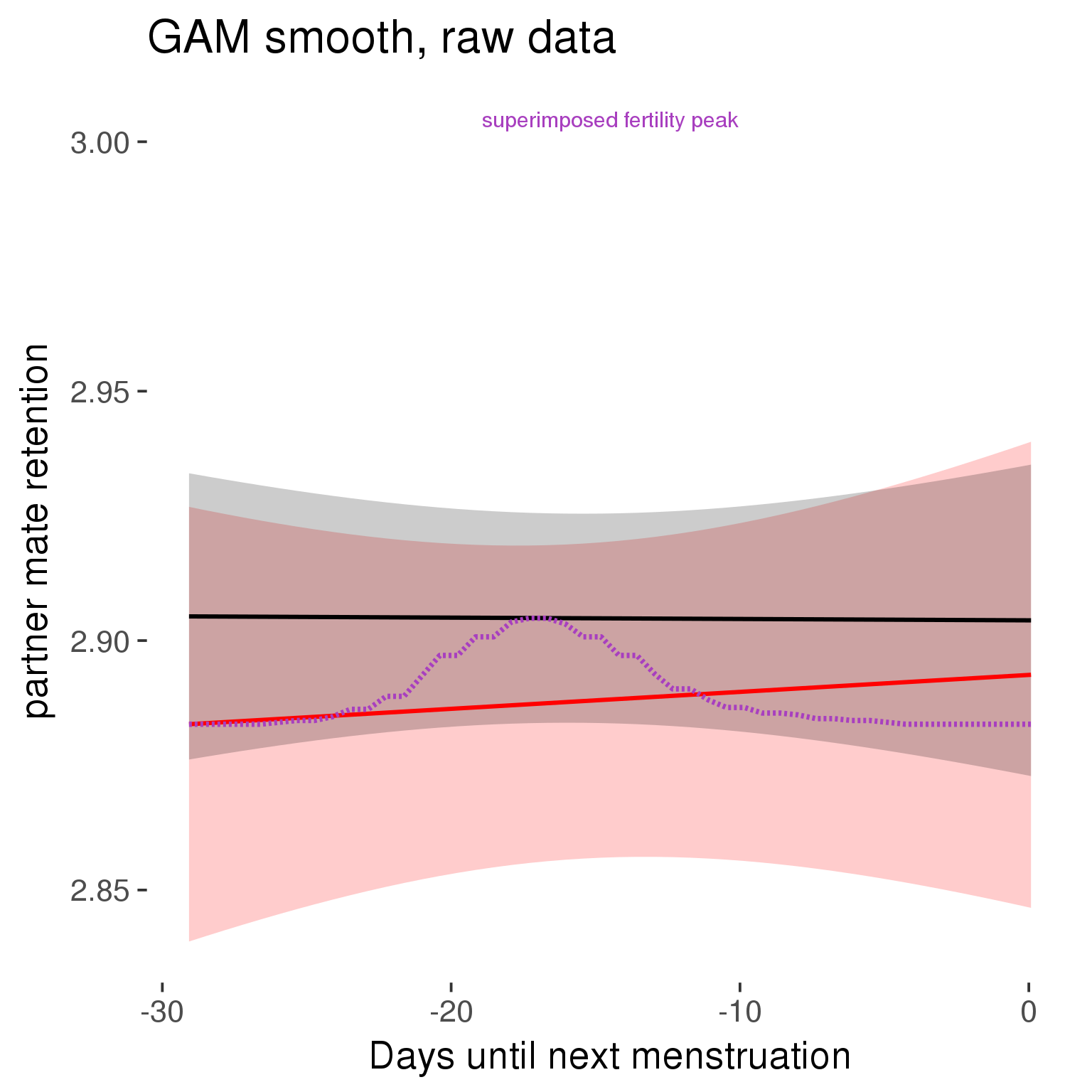
Means and standard errors over raw data
Nothing partialled out, just straight means with bootstrapped confidence intervals.
tryCatch({
trend_plot = ggplot(tmp,aes_string(x = "RCD", y = outcome, colour = "included")) +
geom_pointrange(size = 0.8, stat = 'summary', fun.data = "mean_cl_boot")
}, error = function(e){cat_message(e, "danger")})
tryCatch({
trend_data = ggplot_build(trend_plot)$data[[1]]
}, error = function(e){cat_message(e, "danger")})
trend_data$RCD = round(trend_data$x)
trend_data = left_join(trend_data, tmp %>% select(real, RCD,fertile) %>% unique(), by = "RCD")
trend_data %>%
filter(real == TRUE) %>%
mutate(superimposed = ( ( (fertile - 0.01)/0.58) * (max(y)-min(y) ) ) + min(y) ) ->
trend_data
plot3 = ggplot(trend_data) +
geom_pointrange(aes(x = x, y = y, ymin = ymin,ymax = ymax, colour = factor(group)), size = 0.8, stat = "identity", alpha = 0.6, position = position_dodge(width = .5)) +
scale_x_continuous("Days until next menstruation") +
geom_line(aes(x= x, y = superimposed), color = "#a83fbf", size = 1, linetype = 'dashed') +
annotate("text",x = mean(trend_data$x), y = max(trend_data$superimposed,na.rm=T) + 0.1, label = 'superimposed fertility peak', color = "#a83fbf") +
scale_y_continuous(outcome_label) +
ggtitle("Means with standard errors, raw data") +
scale_color_manual("Contraception status",values = c("2"="black","1"= "red"), labels = c("2"="hormonally\ncontracepting","1"="cycling"), guide = F) +
scale_fill_manual("Contraception status",values = c("2"="black","1"= "red"), labels = c("2"="hormonally\ncontracepting","1"="cycling"), guide = F)
suppressWarnings(print(plot3))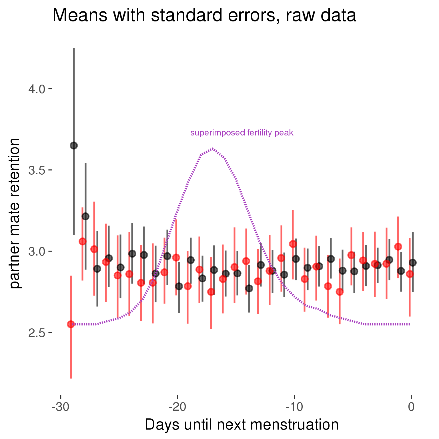
Forward-counted
model %>%
plot_curve(diary %>% filter(minimum_cycle_length_diary <= 30, minimum_cycle_length_diary >= 27) %>% mutate(RCD = FCD, fertile = prc_stirn_b_forward_counted), caption_x = "Days since last menstruation")outcome = names(model@frame)[1]
outcome_label = recode(str_replace_all(str_replace_all(str_replace_all(outcome, "_", " "), " pair", "-pair"), " 1", ""),
"desirability 1" = "self-perceived desirability",
"NARQ admiration" = "narcissistic admiration",
"NARQ rivalry" = "narcissistic rivalry",
"extra-pair" = "extra-pair desire & behaviour",
"had sexual intercourse" = "sexual intercourse")
library(ggplot2)
# form a subset and run the model without the hormonal contraception and the fertility predictors
tmp = diary %>%
filter(!is.na(fertile), !is.na(included),
RCD > -1 * minimum_cycle_length_diary, RCD > -40)
new_form = update.formula(formula(model), new = . ~ . - fertile * included)
tmp$residuals = residuals(update(model, new_form, data = tmp , na.action = na.exclude))
tmp = tmp %>%
filter(!is.na(RCD), !is.na(residuals))
rcd_min = min(tmp$RCD)
tmp$real = FALSE
tmp_before = tmp
tmp_before$RCD = tmp_before$RCD + min(tmp$RCD) - 1
tmp_after = tmp
tmp_after$RCD = tmp_after$RCD - min(tmp$RCD) + 1
tmp$real = TRUE
tmp = bind_rows(tmp_before %>% filter(RCD > rcd_min - 11), tmp, tmp_after %>% filter(RCD < 11))GAM smooth on residuals
Here, we partialled out menstruation and individual random effects, then superimposed estimated probability of being in the fertile window scaled to the range of the estimated means. To address the periodicity of the cycle, we prepended and appended ten days of the timeseries to the end and the beginning of the timeseries. We then estimated the GAM and cut off the appended subsets before plotting.
tryCatch({
trend_plot = ggplot(tmp,aes(x = RCD, y = residuals, colour = included)) +
stat_smooth(geom = 'smooth',size = 0.8, fill = "#9ECAE1", method = 'gam', formula = y ~ s(x))
}, error = function(e){cat_message(e, "danger")})
tryCatch({
trend_data = ggplot_build(trend_plot)$data[[1]]
}, error = function(e){cat_message(e, "danger")})
trend_data$RCD = round(trend_data$x)
trend_data = left_join(trend_data, tmp %>% select(real, RCD,fertile) %>% unique(), by = "RCD")
trend_data %>%
filter(real == TRUE) %>%
mutate(superimposed = ( ( (fertile - 0.01)/0.58) * (max(y)-min(y) ) ) + min(y) ) ->
trend_data
ggplot(trend_data) +
geom_ribbon(aes(x = x, ymin = ymin, ymax = ymax, fill = factor(group)), alpha = 0.2) +
geom_line(aes(x = x, y = y, colour = factor(group)), size = 0.8, stat = "identity") +
scale_x_continuous(caption_x) +
geom_line(aes(x = x, y = superimposed), color = "#a83fbf", size = 1, linetype = 'dashed') +
annotate("text",x = mean(trend_data$x), y = max(trend_data$superimposed,na.rm=T) + 0.1, label = 'superimposed fertility peak', color = "#a83fbf") +
scale_y_continuous(outcome_label) +
ggtitle("GAM smooth, residuals") +
scale_color_manual("Contraception status",values = c("2"="black","1"= "red"), labels = c("2"="hormonally\ncontracepting","1"="cycling"), guide = F) +
scale_fill_manual("Contraception status",values = c("2"="black","1"= "red"), labels = c("2"="hormonally\ncontracepting","1"="cycling"), guide = F)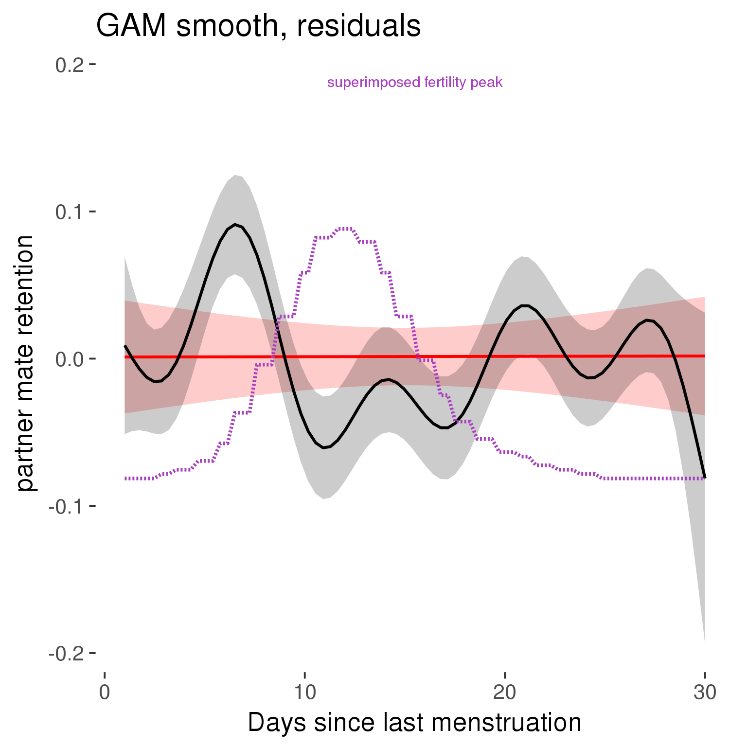
GAM smooth on raw data
As before, but without partialling anything out.
tryCatch({
trend_plot = ggplot(tmp,aes_string(x = "RCD", y = outcome, colour = "included")) +
stat_smooth(geom = 'smooth',size = 0.8, fill = "#9ECAE1", method = 'gam', formula = y ~ s(x))
}, error = function(e){cat_message(e, "danger")})
tryCatch({
trend_data = ggplot_build(trend_plot)$data[[1]]
}, error = function(e){cat_message(e, "danger")})
trend_data$RCD = round(trend_data$x)
trend_data = left_join(trend_data, tmp %>% select(real, RCD,fertile) %>% unique(), by = "RCD")
trend_data %>%
filter(real == TRUE) %>%
mutate(superimposed = ( ( (fertile - 0.01)/0.58) * (max(y)-min(y) ) ) + min(y) ) ->
trend_data
plot1b = ggplot(trend_data) +
geom_ribbon(aes(x = x, ymin = ymin, ymax = ymax, fill = factor(group)), alpha = 0.2) +
geom_line(aes(x = x, y = y, colour = factor(group)), size = 0.8, stat = "identity") +
scale_x_continuous(caption_x) +
geom_line(aes(x = x, y = superimposed), color = "#a83fbf", size = 1, linetype = 'dashed') +
annotate("text",x = mean(trend_data$x), y = max(trend_data$superimposed,na.rm=T) + 0.1, label = 'superimposed fertility peak', color = "#a83fbf") +
scale_y_continuous(outcome_label) +
ggtitle("GAM smooth, raw data") +
scale_color_manual("Contraception status",values = c("2"="black","1"= "red"), labels = c("2"="hormonally\ncontracepting","1"="cycling"), guide = F) +
scale_fill_manual("Contraception status",values = c("2"="black","1"= "red"), labels = c("2"="hormonally\ncontracepting","1"="cycling"), guide = F)
suppressWarnings(print(plot1b))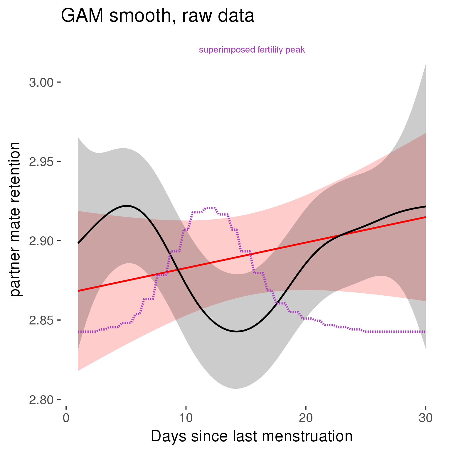
Means and standard errors over raw data
Nothing partialled out, just straight means with bootstrapped confidence intervals.
tryCatch({
trend_plot = ggplot(tmp,aes_string(x = "RCD", y = outcome, colour = "included")) +
geom_pointrange(size = 0.8, stat = 'summary', fun.data = "mean_cl_boot")
}, error = function(e){cat_message(e, "danger")})
tryCatch({
trend_data = ggplot_build(trend_plot)$data[[1]]
}, error = function(e){cat_message(e, "danger")})
trend_data$RCD = round(trend_data$x)
trend_data = left_join(trend_data, tmp %>% select(real, RCD,fertile) %>% unique(), by = "RCD")
trend_data %>%
filter(real == TRUE) %>%
mutate(superimposed = ( ( (fertile - 0.01)/0.58) * (max(y)-min(y) ) ) + min(y) ) ->
trend_data
plot3 = ggplot(trend_data) +
geom_pointrange(aes(x = x, y = y, ymin = ymin,ymax = ymax, colour = factor(group)), size = 0.8, stat = "identity", alpha = 0.6, position = position_dodge(width = .5)) +
scale_x_continuous("Days until next menstruation") +
geom_line(aes(x= x, y = superimposed), color = "#a83fbf", size = 1, linetype = 'dashed') +
annotate("text",x = mean(trend_data$x), y = max(trend_data$superimposed,na.rm=T) + 0.1, label = 'superimposed fertility peak', color = "#a83fbf") +
scale_y_continuous(outcome_label) +
ggtitle("Means with standard errors, raw data") +
scale_color_manual("Contraception status",values = c("2"="black","1"= "red"), labels = c("2"="hormonally\ncontracepting","1"="cycling"), guide = F) +
scale_fill_manual("Contraception status",values = c("2"="black","1"= "red"), labels = c("2"="hormonally\ncontracepting","1"="cycling"), guide = F)
suppressWarnings(print(plot3))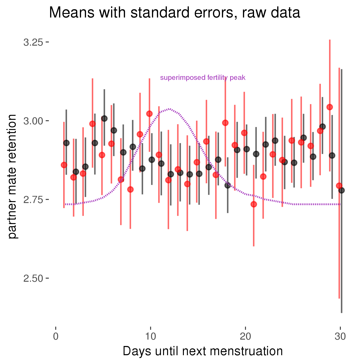
Robustness checks
M_r1: Random slopes for conception risk and menstruation
tryCatch({
# refit model with random effects for fertile and menstruation dummies
with_ind_diff = update(model, formula = . ~ . - (1| person) + (1 + fertile + menstruation | person))
# pull the random effects, format as tibble
rand = coef(with_ind_diff)$person %>%
tibble::rownames_to_column("person") %>%
mutate(person = as.numeric(person))
# pull the fixed effects
fixd = data.frame(fixef(with_ind_diff)) %>%
tibble::rownames_to_column("effect")
names(fixd) = c("effect", "pop_effect_size")
# pull apart the coefficients so that we can account for the fact that the random effect variation implicitly includes HC explaining the mean population-level effect of fertile/menstruation dummies among HC users
fixd = fixd %>%
separate(effect, c("included", "effect"), sep = ":", fill = "left") %>%
mutate(included = if_else(is.na(included), "cycling", str_replace(included, "included", "")))
fixd[2,c("included", "effect")] = c("horm_contra", "(Intercept)")
rand = rand %>%
# merge diary data on the random effects, so that we know who is a HC users and who isn't
inner_join(diary %>% select(person, included) %>% unique(), by = 'person') %>%
# gather into long format, to have the dataset by predictor
gather(effect, value, -person, -included) %>%
inner_join(fixd, by = c('effect', 'included')) %>%
# pull the fixed effects
mutate(
# only for those who are HC users, add the moderated population effect size for this effect (the random effects have the reference category mean)
value = if_else(included == "horm_contra", value + pop_effect_size, value),
effect = recode(effect, "includedhorm_contra" = "HC user",
"includedhorm_contra:fertile" = "HC user x fertile",
"includedhorm_contra:menstruationpre" = "HC user x premens.",
"includedhorm_contra:menstruationyes" = "HC user x mens.",
"menstruationyes" = "mens.",
"menstruationpre" = "premens.")) %>%
group_by(included, effect) %>%
# filter out predictors that aren't modelled as varying/random
filter(sd(value) > 0)
# plot dot plot of random effects
print(
ggplot(rand, aes(x = included, y = value, color = included, fill = included)) +
facet_wrap( ~ effect, scales = "free") +
# geom_violin(alpha = 0.4, size = 0) +
geom_dotplot(binaxis='y', dotsize = 0.1, method = "histodot") +
# geom_jitter(alpha = 0.05) +
coord_flip() +
geom_pointrange(stat = 'summary', fun.data = 'mean_sdl', color = 'darkred', size = 1.2) +
scale_color_manual("Contraception status", values = c("horm_contra"="black","cycling"= "red"), labels = c("horm_contra"="hormonally\ncontracepting","cycling"="cycling"), guide = F) +
scale_fill_manual("Contraception status", values = c("horm_contra"="black","cycling"= "red"), labels = c("horm_contra"="hormonally\ncontracepting","1"="cycling"), guide = F) +
ggtitle("M_r1: allowing participant-varying slopes", subtitle = "for the conception risk measure and the menstruation dummies") +
scale_x_discrete("Hormonal contraception", breaks = c("horm_contra", "cycling"), labels = c("yes", "no")) +
scale_y_continuous("Random effect size distribution"))
print_summary(with_ind_diff)
cat(pander(anova(model, with_ind_diff)))
}, error = function(e){
with_ind_diff = model
cat_message(e, "danger")
})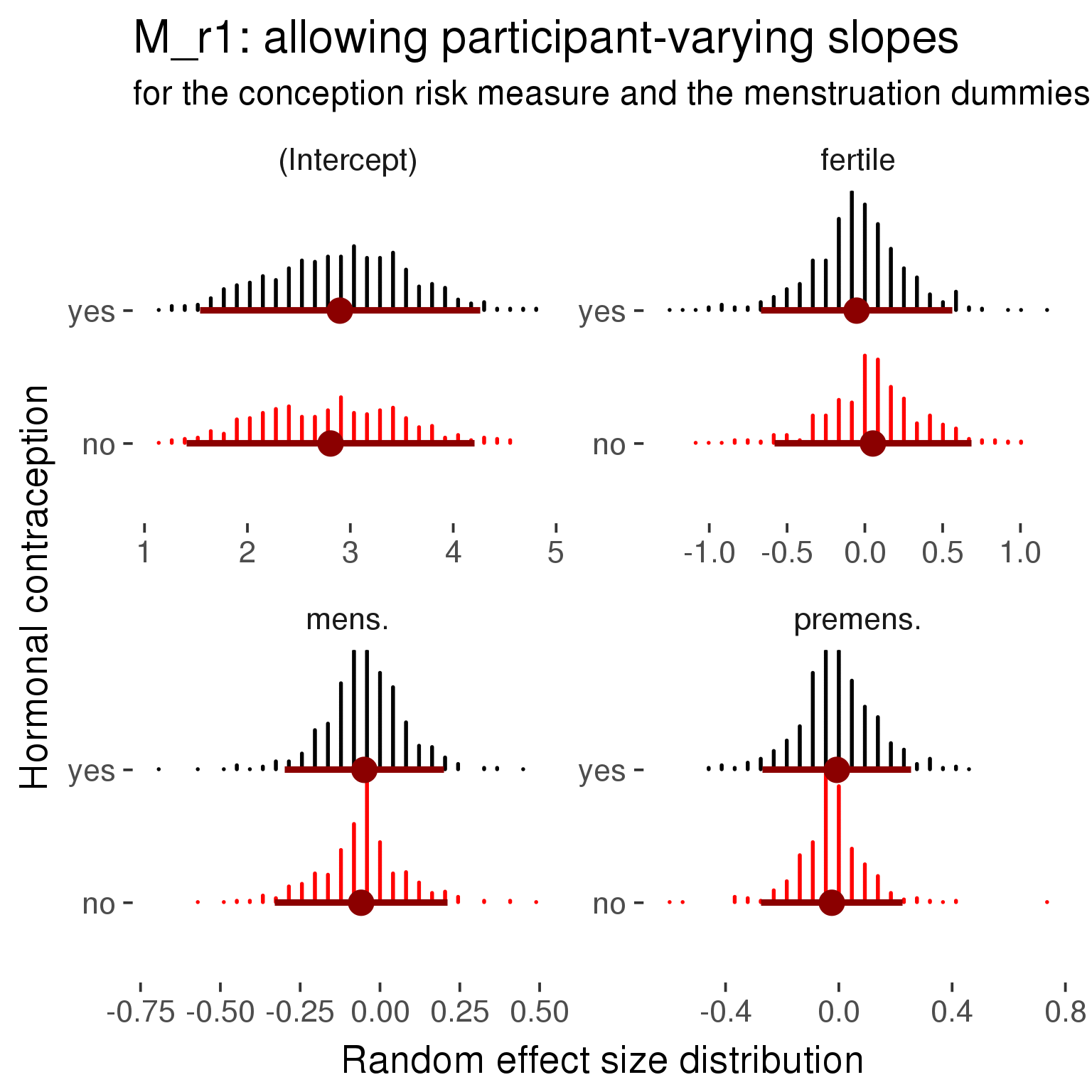
Linear mixed model fit by REML ['lmerMod']
Formula: partner_mate_retention ~ included + menstruation + fertile +
fertile_mean + (1 + fertile + menstruation | person) + included:menstruation + included:fertile
Data: diary
REML criterion at convergence: 66746
Scaled residuals:
Min 1Q Median 3Q Max
-4.755 -0.593 0.006 0.594 4.998
Random effects:
Groups Name Variance Std.Dev. Corr
person (Intercept) 0.5415 0.736
fertile 0.3614 0.601 -0.09
menstruationpre 0.0736 0.271 -0.07 0.29
menstruationyes 0.0729 0.270 -0.14 0.52 0.53
Residual 0.6162 0.785
Number of obs: 26680, groups: person, 1054
Fixed effects:
Estimate Std. Error t value
(Intercept) 2.8080 0.0630 44.6
includedhorm_contra 0.0903 0.0516 1.7
menstruationpre -0.0248 0.0289 -0.9
menstruationyes -0.0591 0.0275 -2.1
fertile 0.0518 0.0596 0.9
fertile_mean -0.1013 0.2891 -0.4
includedhorm_contra:menstruationpre 0.0180 0.0371 0.5
includedhorm_contra:menstruationyes 0.0101 0.0358 0.3
includedhorm_contra:fertile -0.1048 0.0758 -1.4
Correlation of Fixed Effects:
(Intr) incld_ mnstrtnp mnstrtny fertil frtl_m inclddhrm_cntr:mnstrtnp
inclddhrm_c -0.473
menstrutnpr -0.149 0.188
menstrutnys -0.169 0.213 0.429
fertile -0.145 0.241 0.407 0.423
fertile_men -0.772 -0.026 -0.007 -0.007 -0.067
inclddhrm_cntr:mnstrtnp 0.123 -0.236 -0.779 -0.335 -0.316 -0.004
inclddhrm_cntr:mnstrtny 0.136 -0.264 -0.330 -0.767 -0.324 -0.003 0.419
inclddhrm_cntr:f 0.145 -0.303 -0.320 -0.333 -0.785 0.012 0.406
inclddhrm_cntr:mnstrtny
inclddhrm_c
menstrutnpr
menstrutnys
fertile
fertile_men
inclddhrm_cntr:mnstrtnp
inclddhrm_cntr:mnstrtny
inclddhrm_cntr:f 0.420
refitting model(s) with ML (instead of REML)
| Df | AIC | BIC | logLik | deviance | Chisq | Chi Df | Pr(>Chisq) | |
|---|---|---|---|---|---|---|---|---|
| object | 11 | 66914 | 67004 | -33446 | 66892 | NA | NA | NA |
| ..1 | 20 | 66744 | 66908 | -33352 | 66704 | 187.9 | 9 | 1.158e-35 |
robustness_check_ovu_shift(model, diary)M_e: Exclusion criteria
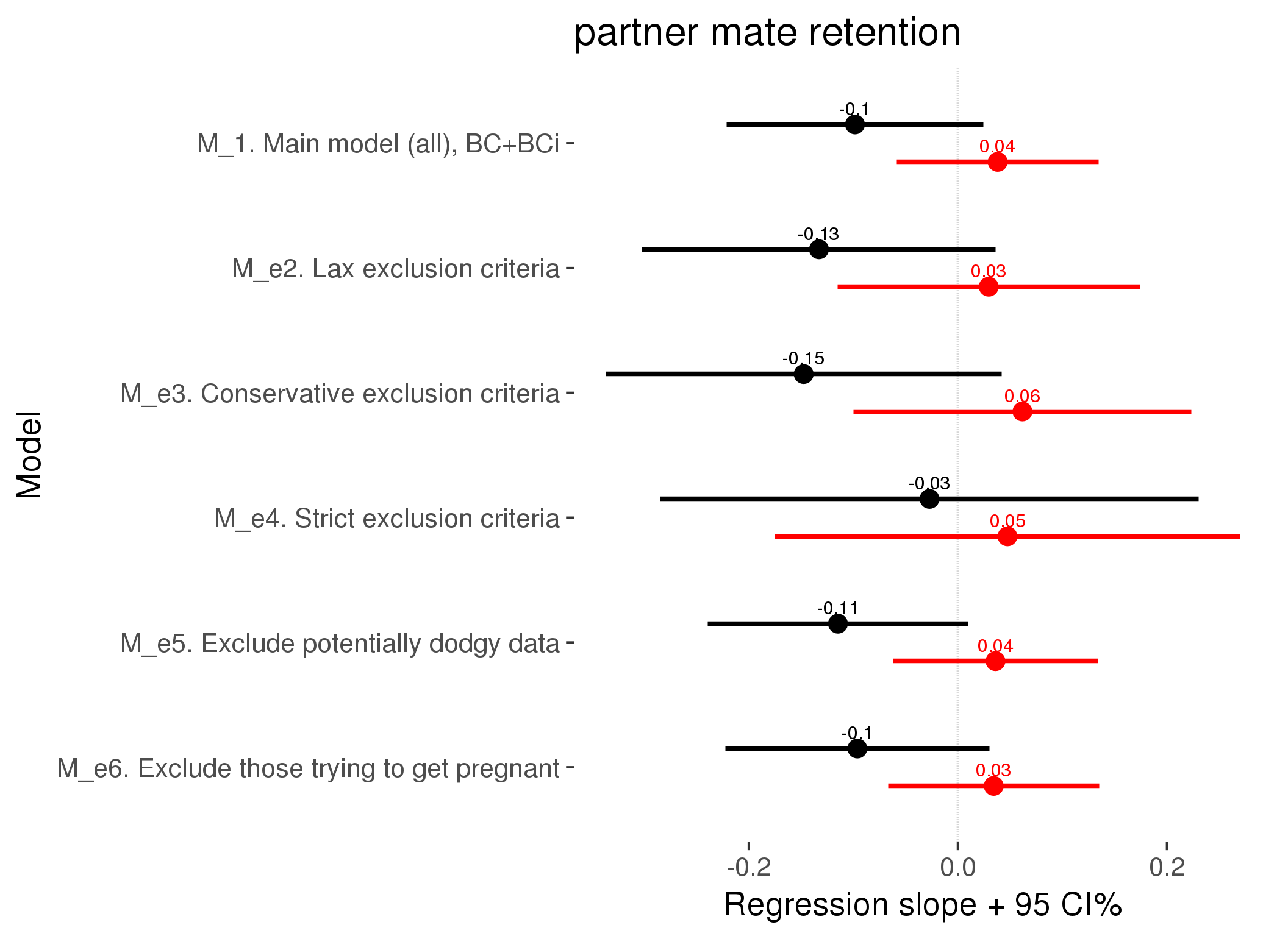
M_p: Predictors
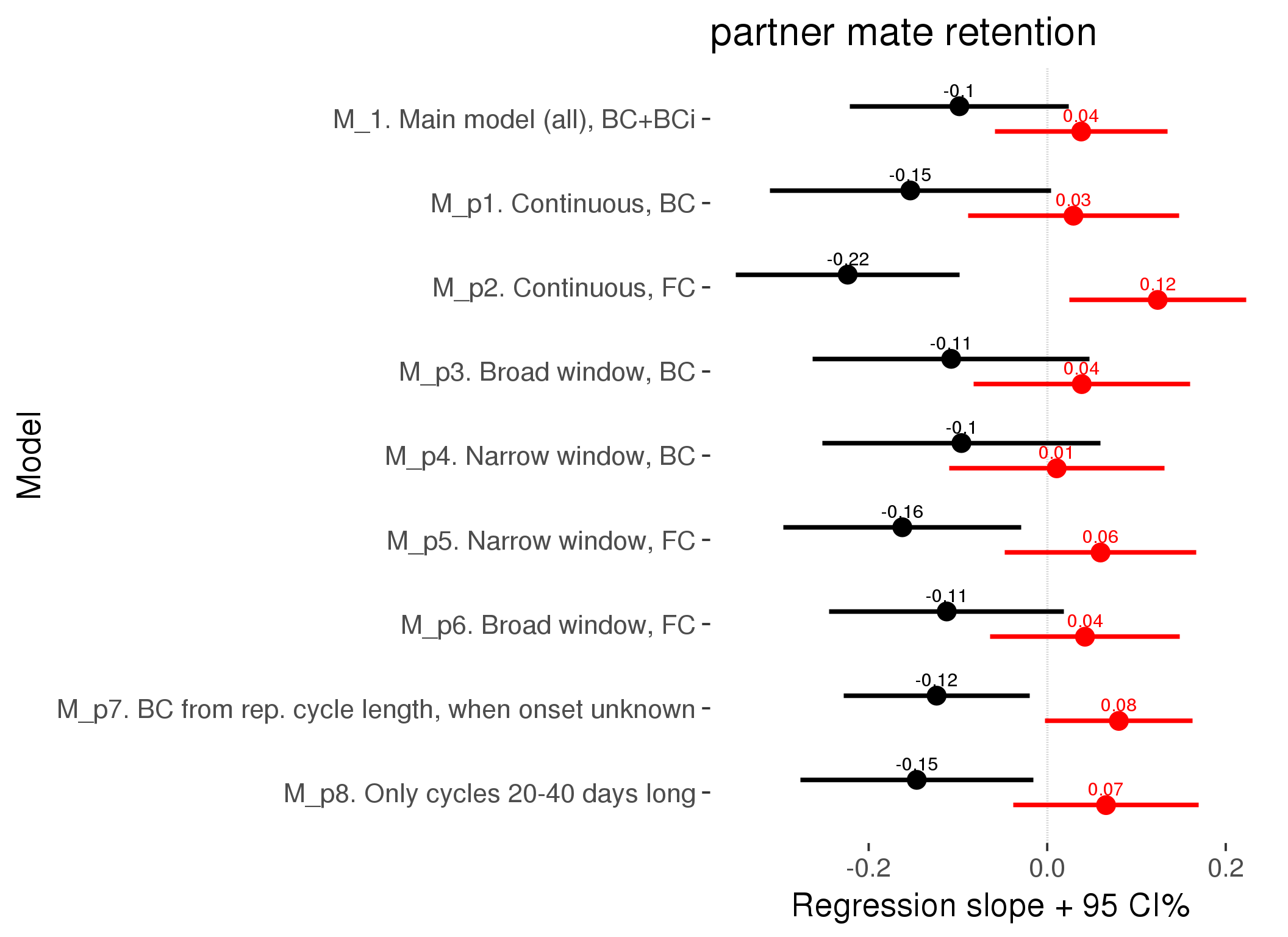
M_c: Covariates, controls, autocorrelation
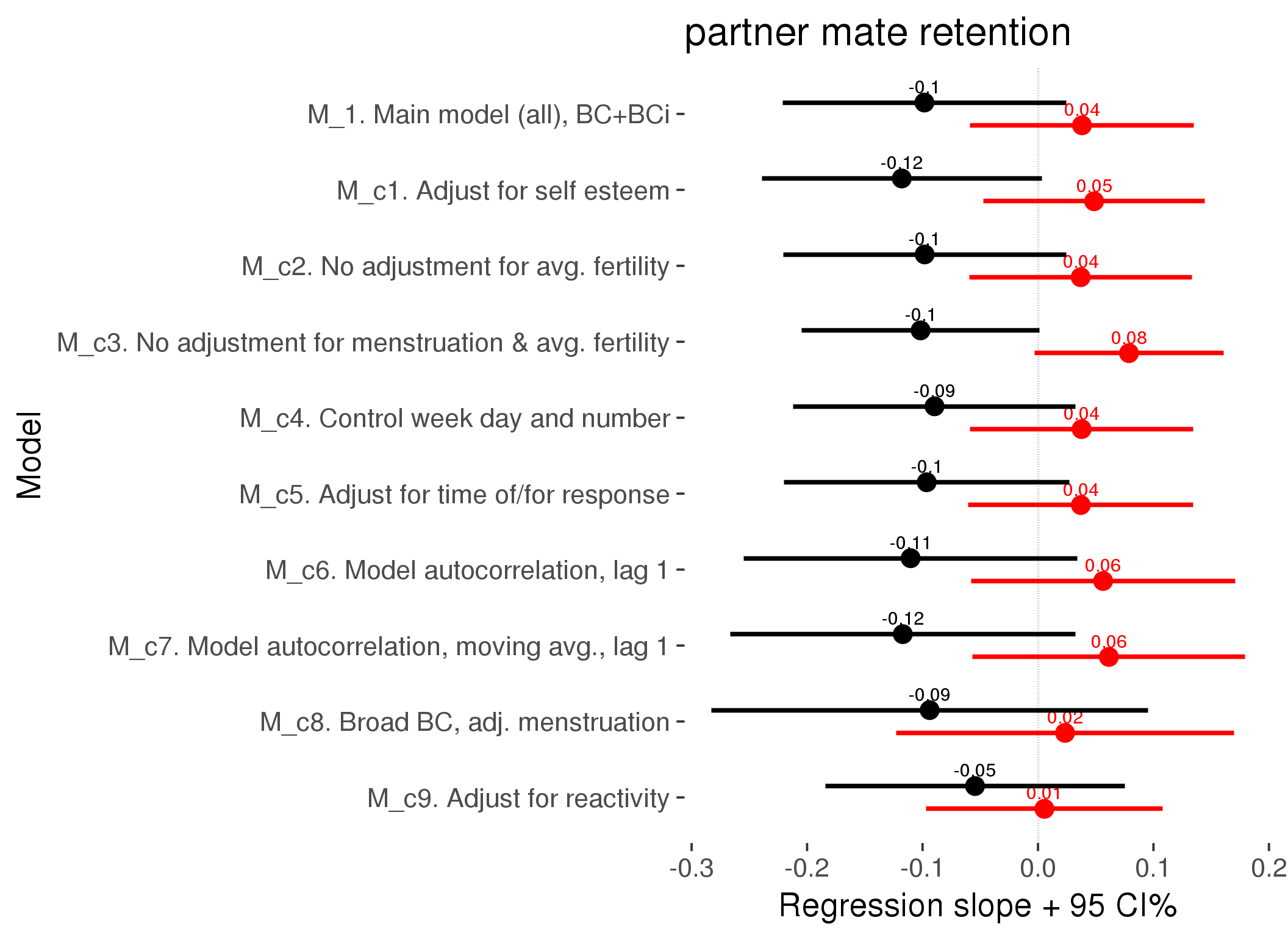
Linear mixed model fit by REML ['lmerMod']
REML criterion at convergence: 60965
Scaled residuals:
Min 1Q Median 3Q Max
-4.714 -0.607 0.013 0.606 4.845
Random effects:
Groups Name Variance Std.Dev.
person (Intercept) 0.5483 0.740
Xr.2 s(days_filled_out):includedhorm_contra 0.0596 0.244
Xr.1 s(days_filled_out):includedcycling 0.0149 0.122
Xr.0 s(day_number):includedhorm_contra 0.0967 0.311
Xr s(day_number):includedcycling 0.0704 0.265
Residual 0.6303 0.794
Number of obs: 24377, groups: person, 1054; Xr.2, 8; Xr.1, 8; Xr.0, 8; Xr, 8
Fixed effects:
Estimate Std. Error t value
X(Intercept) 2.79593 0.06339 44.1
Xincludedhorm_contra 0.08102 0.05239 1.5
Xmenstruationpre -0.02476 0.02537 -1.0
Xmenstruationyes -0.05633 0.02437 -2.3
Xfertile 0.00554 0.05224 0.1
Xfertile_mean -0.05253 0.28813 -0.2
Xincludedhorm_contra:menstruationpre 0.01613 0.03255 0.5
Xincludedhorm_contra:menstruationyes 0.00597 0.03190 0.2
Xincludedhorm_contra:fertile -0.05455 0.06617 -0.8
Xs(day_number):includedcyclingFx1 0.17883 0.08510 2.1
Xs(day_number):includedhorm_contraFx1 0.36978 0.09591 3.9
Xs(days_filled_out):includedcyclingFx1 -0.10987 0.06569 -1.7
Xs(days_filled_out):includedhorm_contraFx1 -0.29722 0.08904 -3.3
Family: gaussian
Link function: identity
Formula:
partner_mate_retention ~ included + menstruation + fertile +
fertile_mean + s(day_number, by = included) + s(days_filled_out,
by = included) + included:menstruation + included:fertile
Parametric coefficients:
Estimate Std. Error t value Pr(>|t|)
(Intercept) 2.79593 0.06339 44.11 <2e-16 ***
includedhorm_contra 0.08102 0.05239 1.55 0.122
menstruationpre -0.02476 0.02537 -0.98 0.329
menstruationyes -0.05633 0.02437 -2.31 0.021 *
fertile 0.00554 0.05224 0.11 0.916
fertile_mean -0.05253 0.28813 -0.18 0.855
includedhorm_contra:menstruationpre 0.01613 0.03255 0.50 0.620
includedhorm_contra:menstruationyes 0.00597 0.03190 0.19 0.851
includedhorm_contra:fertile -0.05455 0.06617 -0.82 0.410
---
Signif. codes: 0 '***' 0.001 '**' 0.01 '*' 0.05 '.' 0.1 ' ' 1
Approximate significance of smooth terms:
edf Ref.df F p-value
s(day_number):includedcycling 3.99 3.99 3.48 0.0083 **
s(day_number):includedhorm_contra 4.54 4.54 7.44 0.0000022 ***
s(days_filled_out):includedcycling 2.19 2.19 2.66 0.0656 .
s(days_filled_out):includedhorm_contra 3.82 3.82 7.87 0.0000047 ***
---
Signif. codes: 0 '***' 0.001 '**' 0.01 '*' 0.05 '.' 0.1 ' ' 1
R-sq.(adj) = 0.00172
lmer.REML = 60965 Scale est. = 0.63032 n = 24377

Linear mixed-effects model fit by REML
Data: diary
AIC BIC logLik
65873 65971 -32925
Random effects:
Formula: ~1 | person
(Intercept) Residual
StdDev: 0.7241 0.8098
Correlation Structure: ARMA(1,0)
Formula: ~day_number | person
Parameter estimate(s):
Phi1
0.2431
Fixed effects: partner_mate_retention ~ included * (menstruation + fertile) + fertile_mean
Value Std.Error DF t-value p-value
(Intercept) 2.8106 0.06343 25620 44.31 0.0000
includedhorm_contra 0.0906 0.05223 1051 1.73 0.0832
menstruationpre -0.0260 0.02777 25620 -0.94 0.3487
menstruationyes -0.0549 0.02597 25620 -2.11 0.0347
fertile 0.0564 0.05825 25620 0.97 0.3330
fertile_mean -0.0866 0.29006 1051 -0.30 0.7654
includedhorm_contra:menstruationpre 0.0150 0.03566 25620 0.42 0.6733
includedhorm_contra:menstruationyes 0.0181 0.03389 25620 0.53 0.5931
includedhorm_contra:fertile -0.1103 0.07373 25620 -1.50 0.1346
Correlation:
(Intr) incld_ mnstrtnp mnstrtny fertil frtl_m inclddhrm_cntr:mnstrtnp
includedhorm_contra -0.477
menstruationpre -0.166 0.210
menstruationyes -0.163 0.204 0.401
fertile -0.160 0.265 0.437 0.367
fertile_mean -0.769 -0.025 -0.008 -0.006 -0.073
includedhorm_contra:menstruationpre 0.137 -0.262 -0.779 -0.312 -0.340 -0.004
includedhorm_contra:menstruationyes 0.131 -0.249 -0.307 -0.766 -0.280 -0.003 0.387
includedhorm_contra:fertile 0.162 -0.335 -0.345 -0.289 -0.787 0.012 0.436
inclddhrm_cntr:mnstrtny
includedhorm_contra
menstruationpre
menstruationyes
fertile
fertile_mean
includedhorm_contra:menstruationpre
includedhorm_contra:menstruationyes
includedhorm_contra:fertile 0.361
Standardized Within-Group Residuals:
Min Q1 Med Q3 Max
-4.598083 -0.617211 0.003373 0.597275 4.753937
Number of Observations: 26680
Number of Groups: 1054
Linear mixed-effects model fit by REML
Data: diary
AIC BIC logLik
65818 65924 -32896
Random effects:
Formula: ~1 | person
(Intercept) Residual
StdDev: 0.7198 0.8128
Correlation Structure: ARMA(1,1)
Formula: ~day_number | person
Parameter estimate(s):
Phi1 Theta1
0.4874 -0.2596
Fixed effects: partner_mate_retention ~ included * (menstruation + fertile) + fertile_mean
Value Std.Error DF t-value p-value
(Intercept) 2.8084 0.06354 25620 44.20 0.0000
includedhorm_contra 0.0923 0.05236 1051 1.76 0.0783
menstruationpre -0.0239 0.02821 25620 -0.85 0.3968
menstruationyes -0.0542 0.02647 25620 -2.05 0.0405
fertile 0.0614 0.06020 25620 1.02 0.3081
fertile_mean -0.0825 0.29070 1051 -0.28 0.7766
includedhorm_contra:menstruationpre 0.0140 0.03624 25620 0.39 0.7002
includedhorm_contra:menstruationyes 0.0162 0.03450 25620 0.47 0.6379
includedhorm_contra:fertile -0.1171 0.07617 25620 -1.54 0.1242
Correlation:
(Intr) incld_ mnstrtnp mnstrtny fertil frtl_m inclddhrm_cntr:mnstrtnp
includedhorm_contra -0.477
menstruationpre -0.168 0.210
menstruationyes -0.166 0.207 0.409
fertile -0.162 0.269 0.418 0.360
fertile_mean -0.769 -0.026 -0.007 -0.006 -0.076
includedhorm_contra:menstruationpre 0.138 -0.263 -0.778 -0.318 -0.324 -0.004
includedhorm_contra:menstruationyes 0.133 -0.253 -0.314 -0.767 -0.276 -0.003 0.395
includedhorm_contra:fertile 0.164 -0.340 -0.330 -0.284 -0.787 0.013 0.417
inclddhrm_cntr:mnstrtny
includedhorm_contra
menstruationpre
menstruationyes
fertile
fertile_mean
includedhorm_contra:menstruationpre
includedhorm_contra:menstruationyes
includedhorm_contra:fertile 0.354
Standardized Within-Group Residuals:
Min Q1 Med Q3 Max
-4.566735 -0.615942 0.005259 0.596748 4.736829
Number of Observations: 26680
Number of Groups: 1054
M_d: Other designs
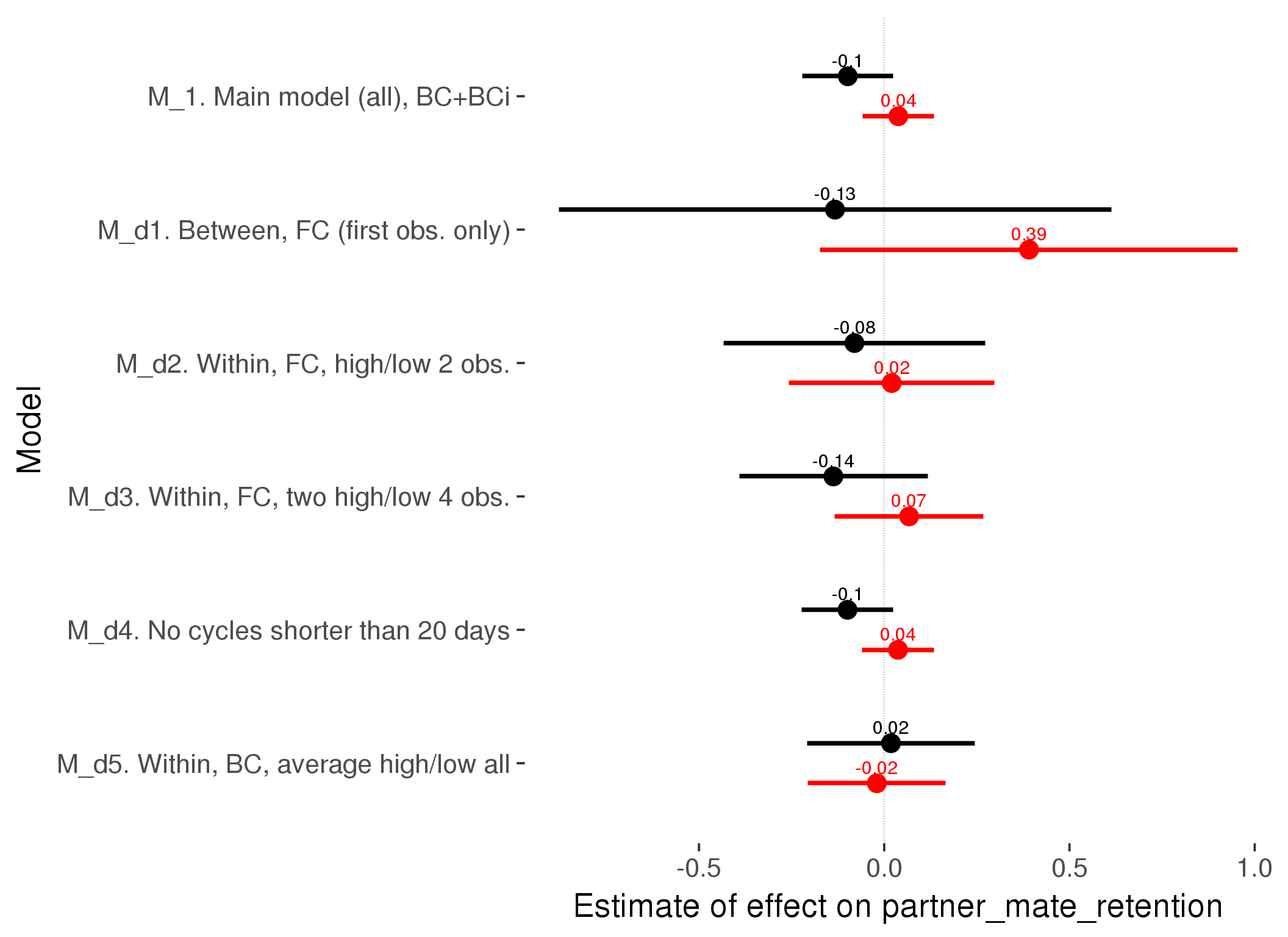
M_m1: Moderation by contraceptive method
Based on the sample with lax exclusion criteria. Users who used any hormonal contraception are classified as hormonal, users who use any awareness-based methods (counting, temperature-based) are classified as ‘fertility-awareness’, women who don’t fall into the before groups and use condoms, pessars, coitus interruptus etc. are classified as ‘barrie or abstinence’. Women who don’t use contraception or use other methods such as sterilisation are excluded from this analysis.
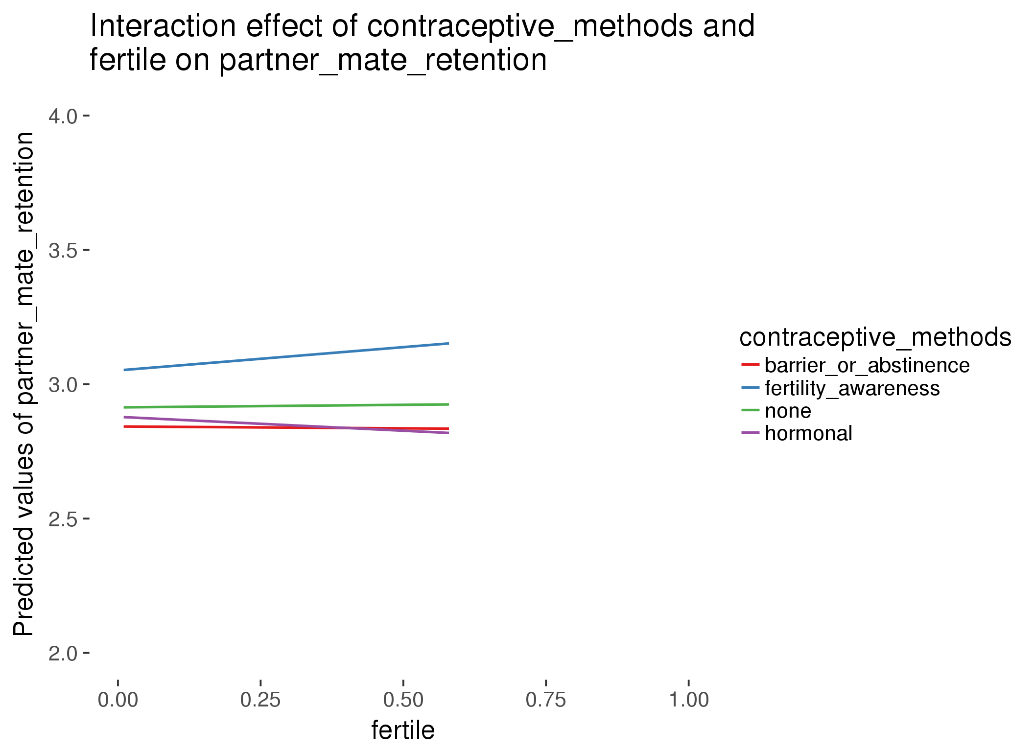
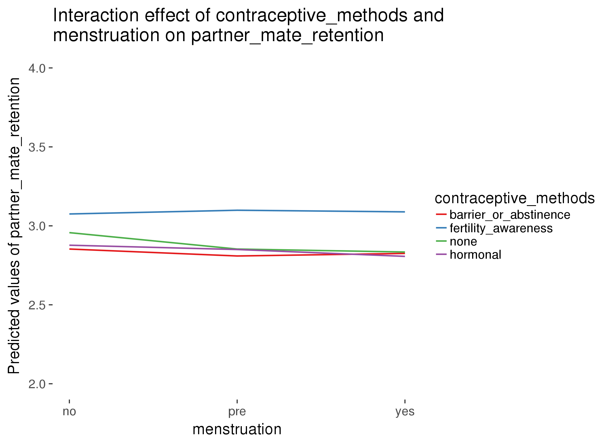
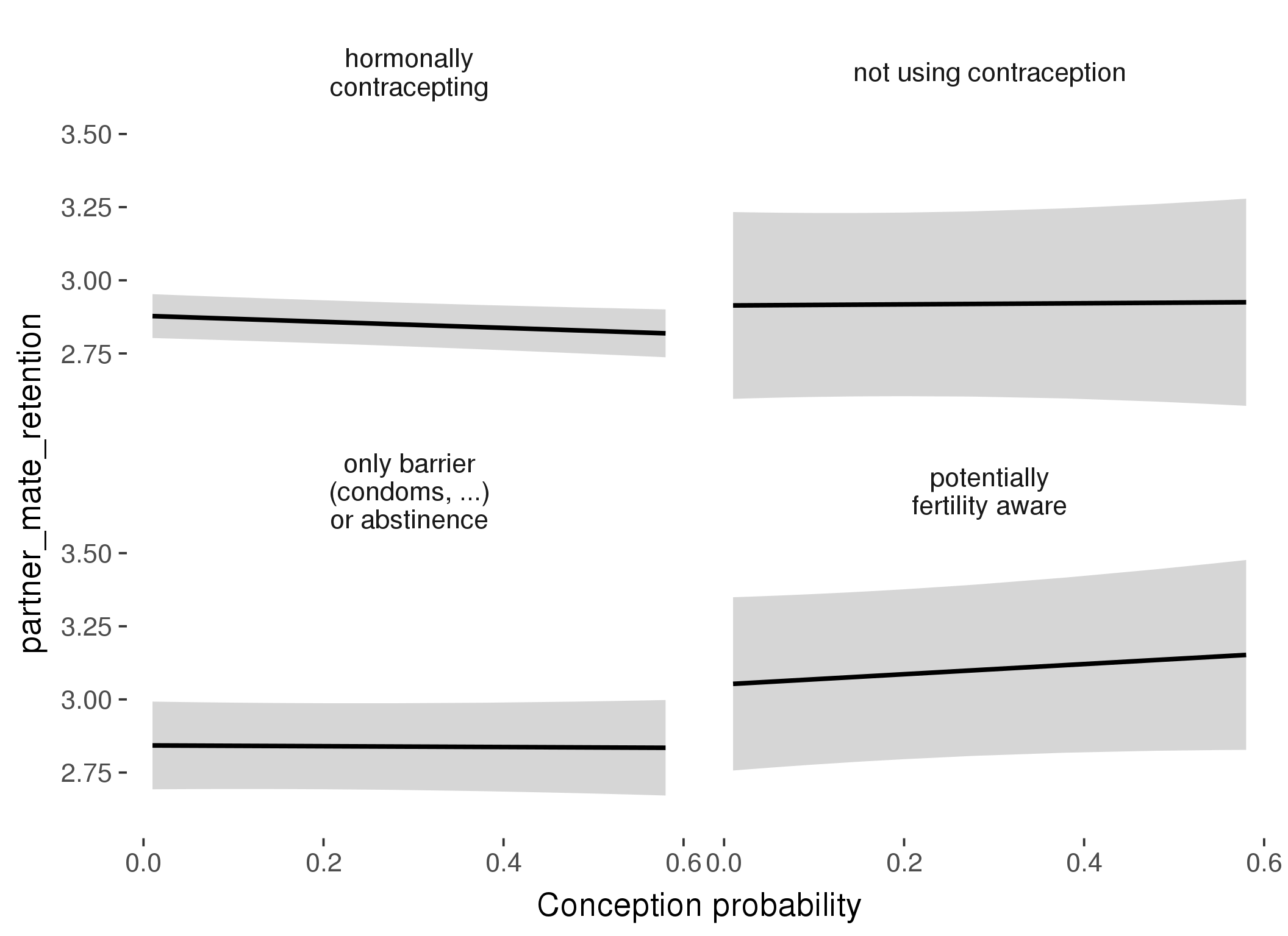
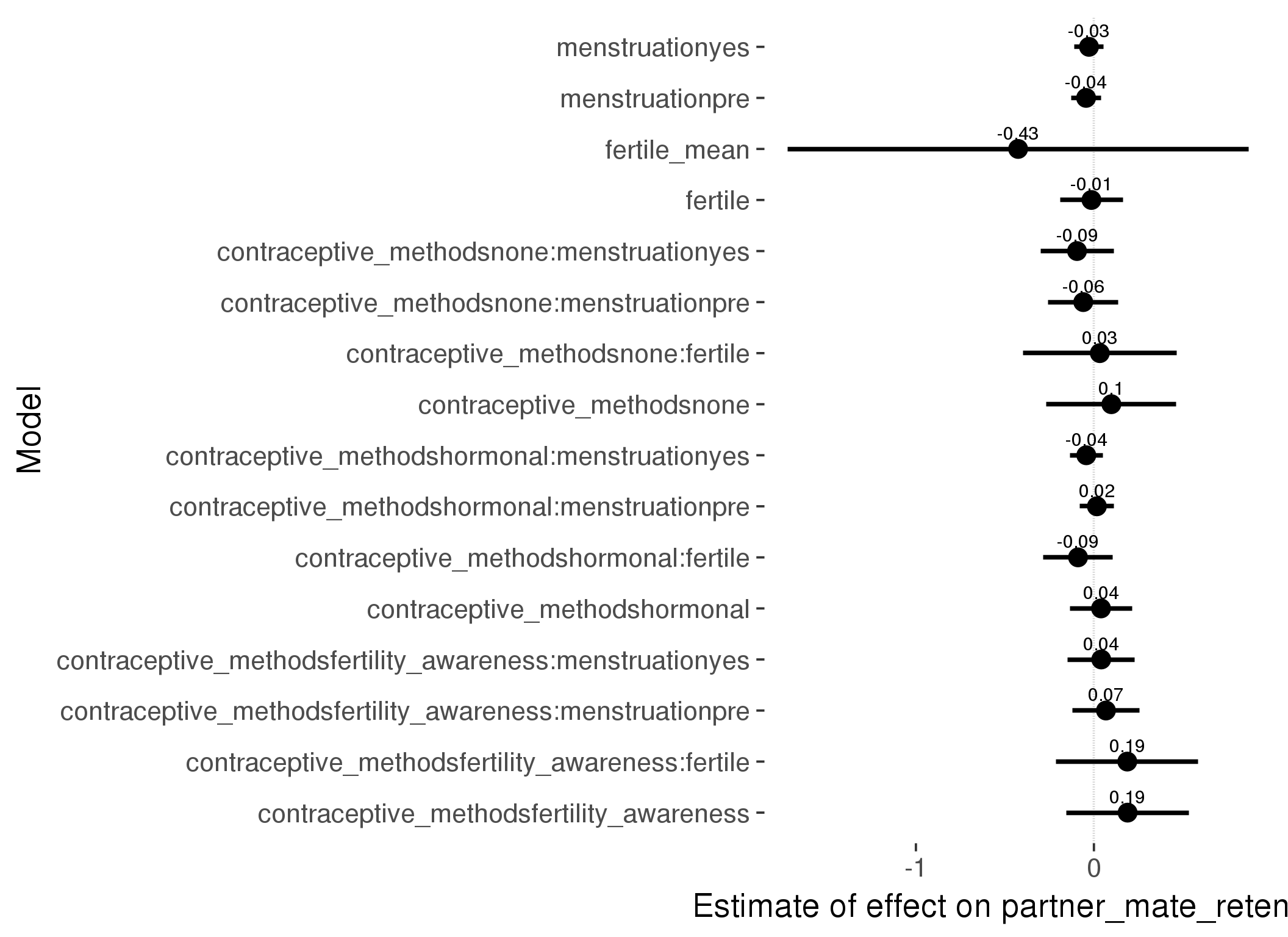
Linear mixed model fit by REML ['lmerMod']
Formula: partner_mate_retention ~ fertile_mean + (1 | person) + contraceptive_methods +
fertile + menstruation + fertile:contraceptive_methods + menstruation:contraceptive_methods
Data: diary
Subset: !is.na(included_lax) & contraceptive_method != "other"
REML criterion at convergence: 42595
Scaled residuals:
Min 1Q Median 3Q Max
-4.677 -0.617 0.021 0.610 4.850
Random effects:
Groups Name Variance Std.Dev.
person (Intercept) 0.506 0.711
Residual 0.646 0.804
Number of obs: 17026, groups: person, 513
Fixed effects:
Estimate Std. Error t value
(Intercept) 2.9302 0.1357 21.59
fertile_mean -0.4258 0.6610 -0.64
contraceptive_methodsfertility_awareness 0.1892 0.1755 1.08
contraceptive_methodsnone 0.0980 0.1860 0.53
contraceptive_methodshormonal 0.0399 0.0885 0.45
fertile -0.0139 0.0897 -0.16
menstruationpre -0.0440 0.0433 -1.02
menstruationyes -0.0278 0.0414 -0.67
contraceptive_methodsfertility_awareness:fertile 0.1874 0.2037 0.92
contraceptive_methodsnone:fertile 0.0330 0.2205 0.15
contraceptive_methodshormonal:fertile -0.0894 0.1002 -0.89
contraceptive_methodsfertility_awareness:menstruationpre 0.0676 0.0959 0.70
contraceptive_methodsnone:menstruationpre -0.0599 0.1003 -0.60
contraceptive_methodshormonal:menstruationpre 0.0167 0.0488 0.34
contraceptive_methodsfertility_awareness:menstruationyes 0.0411 0.0964 0.43
contraceptive_methodsnone:menstruationyes -0.0949 0.1049 -0.91
contraceptive_methodshormonal:menstruationyes -0.0429 0.0472 -0.91
refitting model(s) with ML (instead of REML)
| Df | AIC | BIC | logLik | deviance | Chisq | Chi Df | Pr(>Chisq) | |
|---|---|---|---|---|---|---|---|---|
| add_main | 13 | 42568 | 42669 | -21271 | 42542 | NA | NA | NA |
| by_method | 19 | 42578 | 42725 | -21270 | 42540 | 2.417 | 6 | 0.8777 |
M_m2: Moderation by participant age
model %>%
test_moderator("age_group", diary, xlevels = 5)refitting model(s) with ML (instead of REML)
| Df | AIC | BIC | logLik | deviance | Chisq | Chi Df | Pr(>Chisq) | |
|---|---|---|---|---|---|---|---|---|
| with_main | 19 | 66891 | 67047 | -33426 | 66853 | NA | NA | NA |
| with_mod | 27 | 66886 | 67107 | -33416 | 66832 | 20.63 | 8 | 0.008194 |
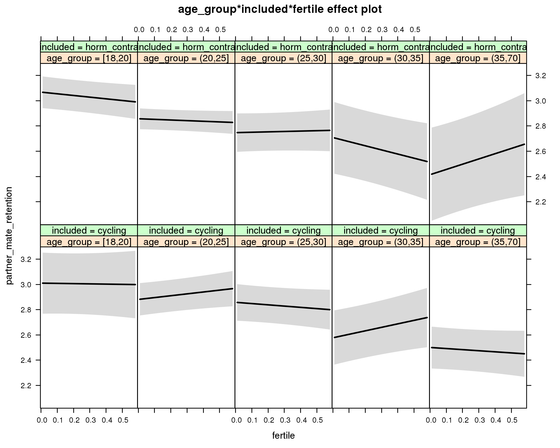
Linear mixed model fit by REML ['lmerMod']
Formula: partner_mate_retention ~ menstruation + fertile_mean + (1 | person) +
age_group + included + fertile + menstruation:included +
age_group:included + age_group:fertile + included:fertile + age_group:included:fertile
Data: diary
REML criterion at convergence: 66915
Scaled residuals:
Min 1Q Median 3Q Max
-4.690 -0.604 0.007 0.614 4.875
Random effects:
Groups Name Variance Std.Dev.
person (Intercept) 0.525 0.724
Residual 0.641 0.801
Number of obs: 26680, groups: person, 1054
Fixed effects:
Estimate Std. Error t value
(Intercept) 3.0495 0.1305 23.37
menstruationpre -0.0327 0.0245 -1.34
menstruationyes -0.0607 0.0231 -2.63
fertile_mean -0.1332 0.2844 -0.47
age_group(20,25] -0.1293 0.1399 -0.92
age_group(25,30] -0.1520 0.1440 -1.06
age_group(30,35] -0.4332 0.1653 -2.62
age_group(35,70] -0.5097 0.1497 -3.41
includedhorm_contra 0.0528 0.1401 0.38
fertile -0.0196 0.1411 -0.14
menstruationpre:includedhorm_contra 0.0197 0.0314 0.63
menstruationyes:includedhorm_contra 0.0117 0.0302 0.39
age_group(20,25]:includedhorm_contra -0.0815 0.1597 -0.51
age_group(25,30]:includedhorm_contra -0.1690 0.1758 -0.96
age_group(30,35]:includedhorm_contra 0.0735 0.2290 0.32
age_group(35,70]:includedhorm_contra -0.1444 0.2494 -0.58
age_group(20,25]:fertile 0.1671 0.1564 1.07
age_group(25,30]:fertile -0.0804 0.1612 -0.50
age_group(30,35]:fertile 0.2961 0.1867 1.59
age_group(35,70]:fertile -0.0667 0.1685 -0.40
includedhorm_contra:fertile -0.1133 0.1565 -0.72
age_group(20,25]:includedhorm_contra:fertile -0.0847 0.1752 -0.48
age_group(25,30]:includedhorm_contra:fertile 0.2441 0.1941 1.26
age_group(30,35]:includedhorm_contra:fertile -0.4912 0.2506 -1.96
age_group(35,70]:includedhorm_contra:fertile 0.6152 0.2846 2.16
M_m3: Moderation by weekend
model %>%
test_moderator("weekend", diary, xlevels = 2) refitting model(s) with ML (instead of REML)
| Df | AIC | BIC | logLik | deviance | Chisq | Chi Df | Pr(>Chisq) | |
|---|---|---|---|---|---|---|---|---|
| with_main | 13 | 66801 | 66908 | -33388 | 66775 | NA | NA | NA |
| with_mod | 15 | 66803 | 66926 | -33387 | 66773 | 2.159 | 2 | 0.3398 |
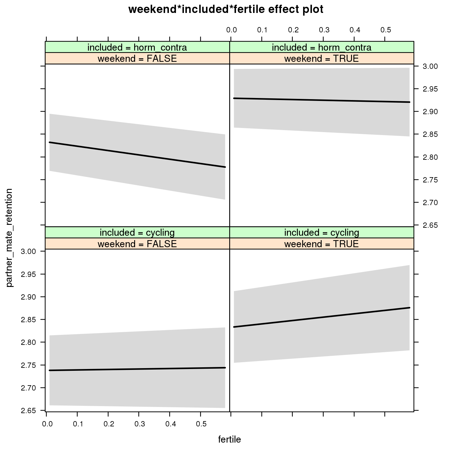
Linear mixed model fit by REML ['lmerMod']
Formula: partner_mate_retention ~ menstruation + fertile_mean + (1 | person) +
weekend + included + fertile + menstruation:included + weekend:included +
weekend:fertile + included:fertile + weekend:included:fertile
Data: diary
REML criterion at convergence: 66837
Scaled residuals:
Min 1Q Median 3Q Max
-4.641 -0.605 0.006 0.608 4.800
Random effects:
Groups Name Variance Std.Dev.
person (Intercept) 0.540 0.735
Residual 0.639 0.799
Number of obs: 26680, groups: person, 1054
Fixed effects:
Estimate Std. Error t value
(Intercept) 2.77107 0.06325 43.8
menstruationpre -0.03163 0.02442 -1.3
menstruationyes -0.06067 0.02301 -2.6
fertile_mean -0.09781 0.28622 -0.3
weekendTRUE 0.09486 0.02127 4.5
includedhorm_contra 0.08907 0.05258 1.7
fertile 0.01023 0.05993 0.2
menstruationpre:includedhorm_contra 0.01979 0.03135 0.6
menstruationyes:includedhorm_contra 0.01489 0.03017 0.5
weekendTRUE:includedhorm_contra 0.00121 0.02738 0.0
weekendTRUE:fertile 0.06420 0.08249 0.8
includedhorm_contra:fertile -0.10579 0.07616 -1.4
weekendTRUE:includedhorm_contra:fertile 0.01659 0.10492 0.2
M_m4: Moderation by weekday
model %>%
test_moderator("weekday", diary, xlevels = 7)refitting model(s) with ML (instead of REML)
| Df | AIC | BIC | logLik | deviance | Chisq | Chi Df | Pr(>Chisq) | |
|---|---|---|---|---|---|---|---|---|
| with_main | 23 | 66754 | 66942 | -33354 | 66708 | NA | NA | NA |
| with_mod | 35 | 66768 | 67055 | -33349 | 66698 | 9.674 | 12 | 0.6445 |
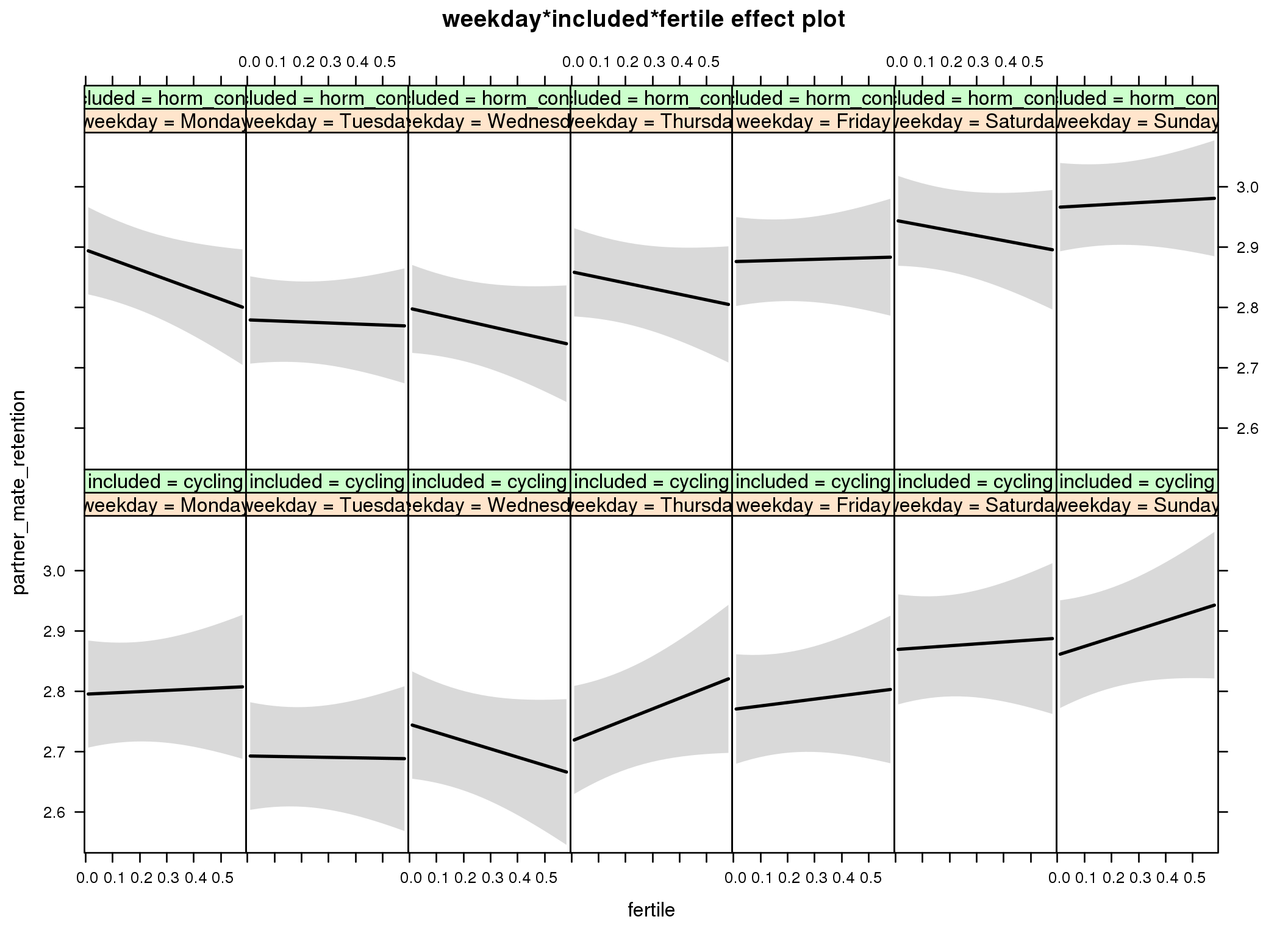
Linear mixed model fit by REML ['lmerMod']
Formula: partner_mate_retention ~ menstruation + fertile_mean + (1 | person) +
weekday + included + fertile + menstruation:included + weekday:included +
weekday:fertile + included:fertile + weekday:included:fertile
Data: diary
REML criterion at convergence: 66842
Scaled residuals:
Min 1Q Median 3Q Max
-4.602 -0.604 0.008 0.607 4.734
Random effects:
Groups Name Variance Std.Dev.
person (Intercept) 0.540 0.735
Residual 0.637 0.798
Number of obs: 26680, groups: person, 1054
Fixed effects:
Estimate Std. Error t value
(Intercept) 2.82969 0.06738 42.0
menstruationpre -0.03161 0.02439 -1.3
menstruationyes -0.06097 0.02299 -2.7
fertile_mean -0.10553 0.28626 -0.4
weekdayTuesday -0.10246 0.03802 -2.7
weekdayWednesday -0.04986 0.03795 -1.3
weekdayThursday -0.07768 0.03839 -2.0
weekdayFriday -0.02516 0.03903 -0.6
weekdaySaturday 0.07391 0.03943 1.9
weekdaySunday 0.06489 0.03810 1.7
includedhorm_contra 0.09412 0.06036 1.6
fertile 0.02093 0.10708 0.2
menstruationpre:includedhorm_contra 0.02041 0.03132 0.7
menstruationyes:includedhorm_contra 0.01577 0.03014 0.5
weekdayTuesday:includedhorm_contra -0.01360 0.04884 -0.3
weekdayWednesday:includedhorm_contra -0.04708 0.04900 -1.0
weekdayThursday:includedhorm_contra 0.04133 0.04947 0.8
weekdayFriday:includedhorm_contra 0.00565 0.05015 0.1
weekdaySaturday:includedhorm_contra -0.02508 0.05073 -0.5
weekdaySunday:includedhorm_contra 0.00561 0.04918 0.1
weekdayTuesday:fertile -0.02852 0.14741 -0.2
weekdayWednesday:fertile -0.15738 0.14809 -1.1
weekdayThursday:fertile 0.15673 0.15021 1.0
weekdayFriday:fertile 0.03580 0.15046 0.2
weekdaySaturday:fertile 0.01049 0.15246 0.1
weekdaySunday:fertile 0.12147 0.14817 0.8
includedhorm_contra:fertile -0.18471 0.13698 -1.3
weekdayTuesday:includedhorm_contra:fertile 0.17516 0.18813 0.9
weekdayWednesday:includedhorm_contra:fertile 0.22009 0.18961 1.2
weekdayThursday:includedhorm_contra:fertile -0.08625 0.19117 -0.5
weekdayFriday:includedhorm_contra:fertile 0.14055 0.19173 0.7
weekdaySaturday:includedhorm_contra:fertile 0.06929 0.19449 0.4
weekdaySunday:includedhorm_contra:fertile 0.06792 0.18927 0.4
M_m5: Moderation by exclusion threshold
model %>%
test_moderator("included_levels", diary, xlevels = 4)refitting model(s) with ML (instead of REML)
| Df | AIC | BIC | logLik | deviance | Chisq | Chi Df | Pr(>Chisq) | |
|---|---|---|---|---|---|---|---|---|
| with_main | 17 | 66917 | 67056 | -33442 | 66883 | NA | NA | NA |
| with_mod | 23 | 66922 | 67110 | -33438 | 66876 | 7.174 | 6 | 0.3051 |
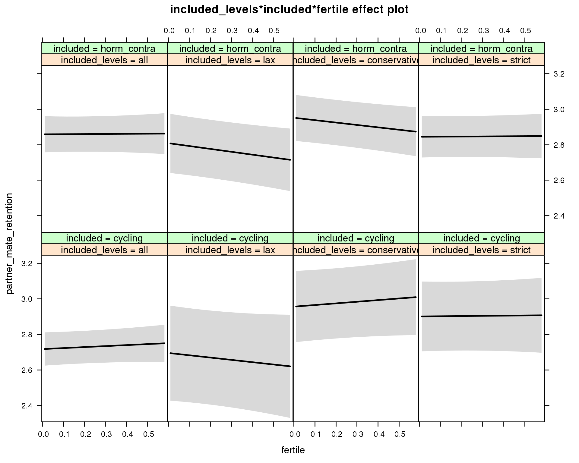
Linear mixed model fit by REML ['lmerMod']
Formula: partner_mate_retention ~ menstruation + fertile_mean + (1 | person) +
included_levels + included + fertile + menstruation:included +
included_levels:included + included_levels:fertile + included:fertile +
included_levels:included:fertile
Data: diary
REML criterion at convergence: 66953
Scaled residuals:
Min 1Q Median 3Q Max
-4.700 -0.607 0.014 0.612 4.882
Random effects:
Groups Name Variance Std.Dev.
person (Intercept) 0.538 0.733
Residual 0.642 0.801
Number of obs: 26680, groups: person, 1054
Fixed effects:
Estimate Std. Error t value
(Intercept) 2.7587 0.0695 39.7
menstruationpre -0.0328 0.0245 -1.3
menstruationyes -0.0597 0.0231 -2.6
fertile_mean -0.1413 0.2882 -0.5
included_levelslax -0.0219 0.1446 -0.2
included_levelsconservative 0.2388 0.1128 2.1
included_levelsstrict 0.1836 0.1110 1.7
includedhorm_contra 0.1348 0.0717 1.9
fertile 0.0560 0.0624 0.9
menstruationpre:includedhorm_contra 0.0211 0.0315 0.7
menstruationyes:includedhorm_contra 0.0115 0.0303 0.4
included_levelslax:includedhorm_contra -0.0280 0.1758 -0.2
included_levelsconservative:includedhorm_contra -0.1457 0.1407 -1.0
included_levelsstrict:includedhorm_contra -0.1976 0.1362 -1.5
included_levelslax:fertile -0.1857 0.1524 -1.2
included_levelsconservative:fertile 0.0361 0.1138 0.3
included_levelsstrict:fertile -0.0450 0.1139 -0.4
includedhorm_contra:fertile -0.0494 0.0955 -0.5
included_levelslax:includedhorm_contra:fertile 0.0174 0.1860 0.1
included_levelsconservative:includedhorm_contra:fertile -0.1776 0.1481 -1.2
included_levelsstrict:includedhorm_contra:fertile 0.0453 0.1458 0.3
M_m6: Moderation by cycle length
model %>%
test_moderator("cycle_length_groups", diary, xlevels = 4)refitting model(s) with ML (instead of REML)
| Df | AIC | BIC | logLik | deviance | Chisq | Chi Df | Pr(>Chisq) | |
|---|---|---|---|---|---|---|---|---|
| with_main | 17 | 66920 | 67060 | -33443 | 66886 | NA | NA | NA |
| with_mod | 23 | 66930 | 67118 | -33442 | 66884 | 2.389 | 6 | 0.8807 |
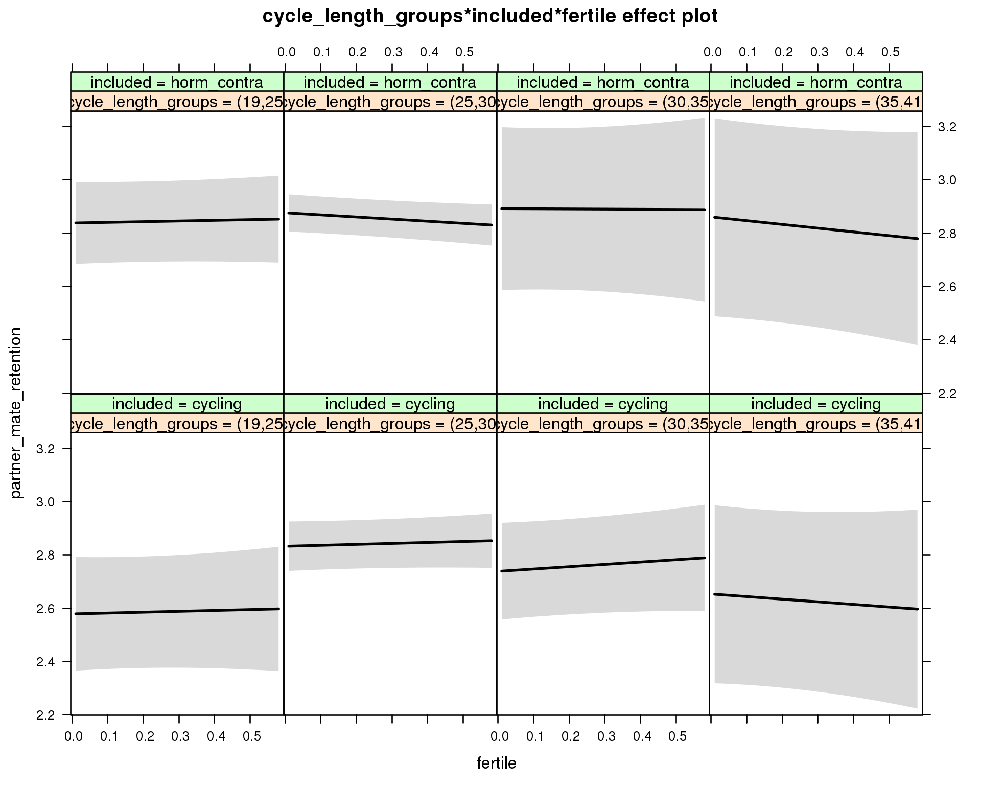
Linear mixed model fit by REML ['lmerMod']
Formula: partner_mate_retention ~ menstruation + fertile_mean + (1 | person) +
cycle_length_groups + included + fertile + menstruation:included +
cycle_length_groups:included + cycle_length_groups:fertile +
included:fertile + cycle_length_groups:included:fertile
Data: diary
REML criterion at convergence: 66953
Scaled residuals:
Min 1Q Median 3Q Max
-4.693 -0.607 0.009 0.611 4.850
Random effects:
Groups Name Variance Std.Dev.
person (Intercept) 0.540 0.735
Residual 0.642 0.801
Number of obs: 26680, groups: person, 1054
Fixed effects:
Estimate Std. Error t value
(Intercept) 2.61632 0.12064 21.69
menstruationpre -0.03137 0.02451 -1.28
menstruationyes -0.05964 0.02324 -2.57
fertile_mean -0.12514 0.29001 -0.43
cycle_length_groups(25,30] 0.25375 0.11872 2.14
cycle_length_groups(30,35] 0.15971 0.14295 1.12
cycle_length_groups(35,41] 0.07480 0.20251 0.37
includedhorm_contra 0.25378 0.13489 1.88
fertile 0.03248 0.13038 0.25
menstruationpre:includedhorm_contra 0.02009 0.03145 0.64
menstruationyes:includedhorm_contra 0.01076 0.03042 0.35
cycle_length_groups(25,30]:includedhorm_contra -0.21525 0.14668 -1.47
cycle_length_groups(30,35]:includedhorm_contra -0.10575 0.22545 -0.47
cycle_length_groups(35,41]:includedhorm_contra -0.05199 0.28790 -0.18
cycle_length_groups(25,30]:fertile 0.00341 0.13989 0.02
cycle_length_groups(30,35]:fertile 0.05503 0.16562 0.33
cycle_length_groups(35,41]:fertile -0.13027 0.23393 -0.56
includedhorm_contra:fertile -0.00720 0.15391 -0.05
cycle_length_groups(25,30]:includedhorm_contra:fertile -0.10801 0.16572 -0.65
cycle_length_groups(30,35]:includedhorm_contra:fertile -0.08625 0.26073 -0.33
cycle_length_groups(35,41]:includedhorm_contra:fertile -0.03533 0.30801 -0.11
M_m7: Moderation by certainty about menstruation parameters
model %>%
test_moderator("certainty_menstruation", diary)refitting model(s) with ML (instead of REML)
| Df | AIC | BIC | logLik | deviance | Chisq | Chi Df | Pr(>Chisq) | |
|---|---|---|---|---|---|---|---|---|
| with_main | 13 | 66913 | 67020 | -33444 | 66887 | NA | NA | NA |
| with_mod | 15 | 66911 | 67034 | -33441 | 66881 | 5.939 | 2 | 0.05134 |
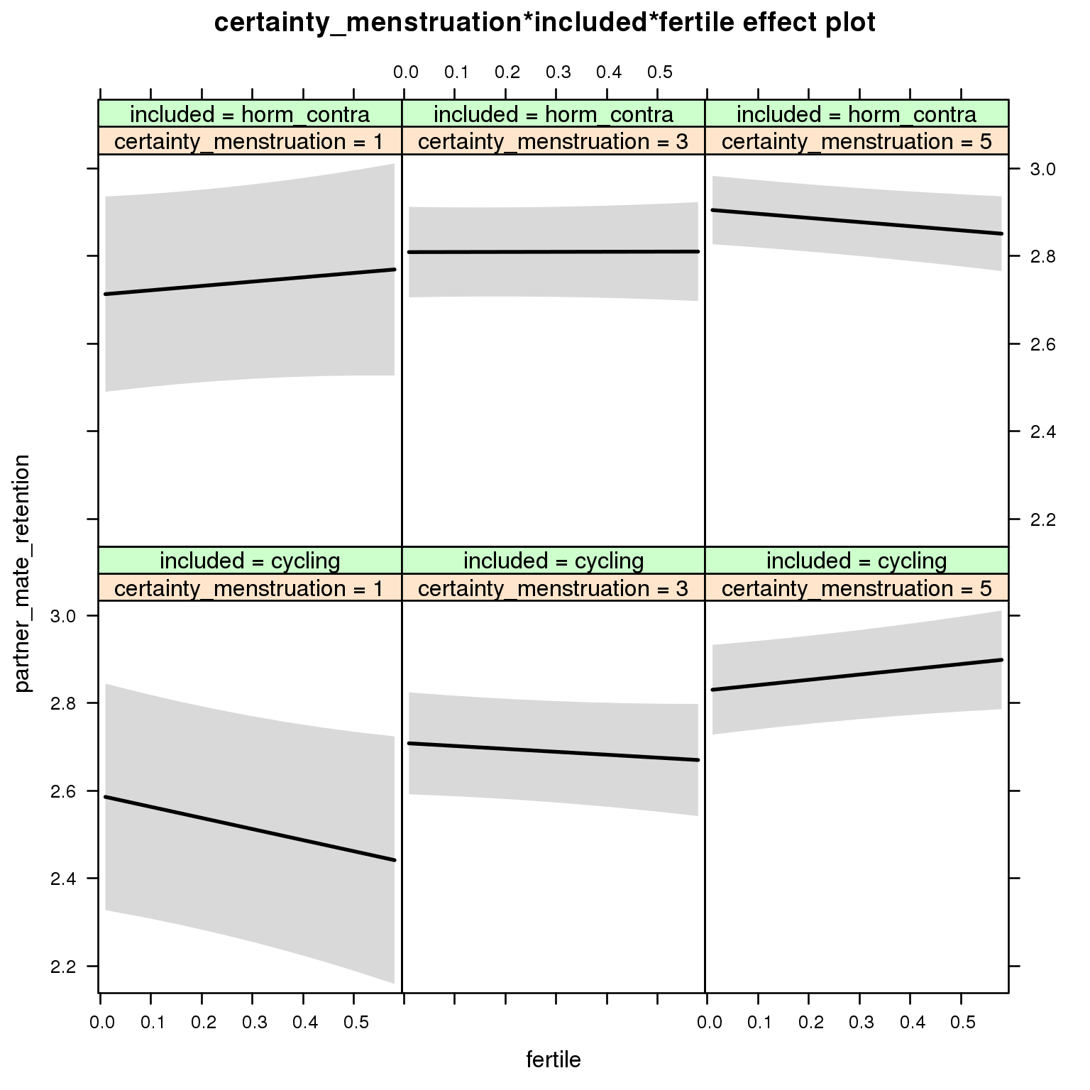
Linear mixed model fit by REML ['lmerMod']
Formula: partner_mate_retention ~ menstruation + fertile_mean + (1 | person) +
certainty_menstruation + included + fertile + menstruation:included +
certainty_menstruation:included + certainty_menstruation:fertile +
included:fertile + certainty_menstruation:included:fertile
Data: diary
REML criterion at convergence: 66944
Scaled residuals:
Min 1Q Median 3Q Max
-4.695 -0.608 0.009 0.610 4.876
Random effects:
Groups Name Variance Std.Dev.
person (Intercept) 0.538 0.734
Residual 0.642 0.801
Number of obs: 26680, groups: person, 1054
Fixed effects:
Estimate Std. Error t value
(Intercept) 2.56593 0.17765 14.44
menstruationpre -0.02992 0.02448 -1.22
menstruationyes -0.05736 0.02310 -2.48
fertile_mean -0.13099 0.28644 -0.46
certainty_menstruation 0.06021 0.04051 1.49
includedhorm_contra 0.13090 0.22560 0.58
fertile -0.34654 0.19438 -1.78
menstruationpre:includedhorm_contra 0.01892 0.03142 0.60
menstruationyes:includedhorm_contra 0.00962 0.03026 0.32
certainty_menstruation:includedhorm_contra -0.01176 0.05257 -0.22
certainty_menstruation:fertile 0.09325 0.04555 2.05
includedhorm_contra:fertile 0.49359 0.25268 1.95
certainty_menstruation:includedhorm_contra:fertile -0.14157 0.05840 -2.42
M_m8: Moderation by cycle regularity
model %>%
test_moderator("cycle_regularity", diary)refitting model(s) with ML (instead of REML)
| Df | AIC | BIC | logLik | deviance | Chisq | Chi Df | Pr(>Chisq) | |
|---|---|---|---|---|---|---|---|---|
| with_main | 15 | 66919 | 67042 | -33445 | 66889 | NA | NA | NA |
| with_mod | 19 | 66915 | 67070 | -33438 | 66877 | 12.44 | 4 | 0.01434 |
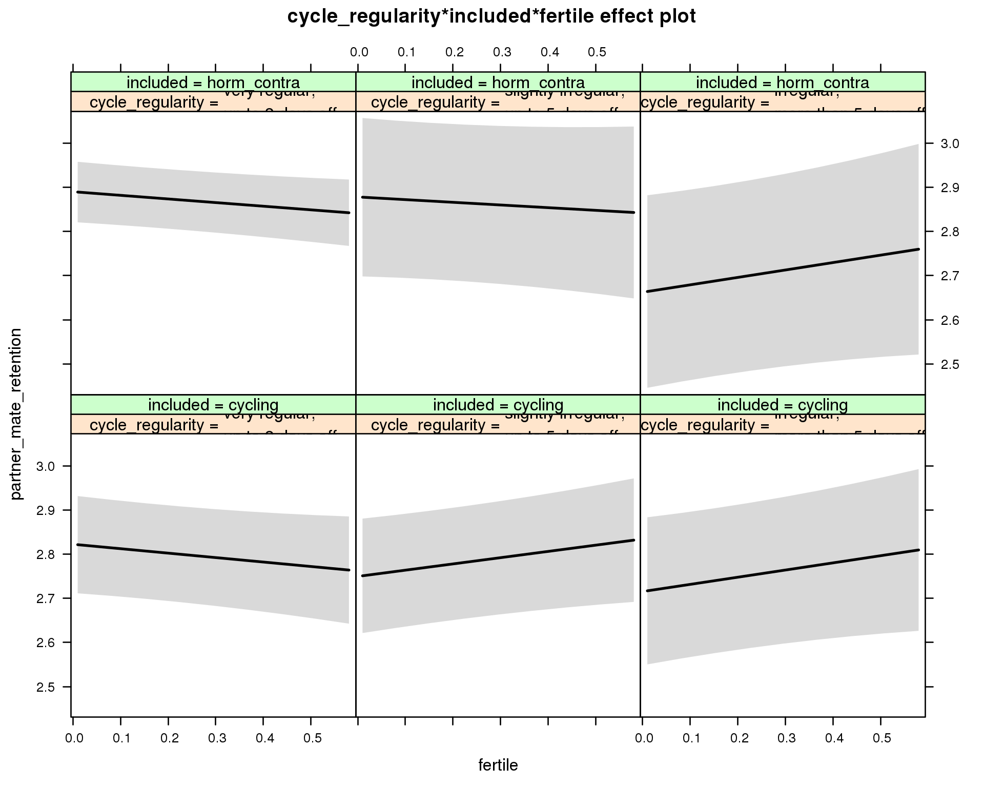
Linear mixed model fit by REML ['lmerMod']
Formula: partner_mate_retention ~ menstruation + fertile_mean + (1 | person) +
cycle_regularity + included + fertile + menstruation:included +
cycle_regularity:included + cycle_regularity:fertile + included:fertile +
cycle_regularity:included:fertile
Data: diary
REML criterion at convergence: 66942
Scaled residuals:
Min 1Q Median 3Q Max
-4.695 -0.607 0.009 0.613 4.874
Random effects:
Groups Name Variance Std.Dev.
person (Intercept) 0.541 0.735
Residual 0.642 0.801
Number of obs: 26680, groups: person, 1054
Fixed effects:
Estimate Std. Error t value
(Intercept) 2.8634 0.0741 38.6
menstruationpre -0.0337 0.0245 -1.4
menstruationyes -0.0613 0.0231 -2.7
fertile_mean -0.1403 0.2879 -0.5
cycle_regularityslightly irregular,\nup to 5 days off -0.0729 0.0868 -0.8
cycle_regularityirregular,\nmore than 5 days off -0.1071 0.1018 -1.1
includedhorm_contra 0.0616 0.0677 0.9
fertile -0.1007 0.0684 -1.5
menstruationpre:includedhorm_contra 0.0220 0.0314 0.7
menstruationyes:includedhorm_contra 0.0129 0.0302 0.4
cycle_regularityslightly irregular,\nup to 5 days off:includedhorm_contra 0.0610 0.1311 0.5
cycle_regularityirregular,\nmore than 5 days off:includedhorm_contra -0.1206 0.1549 -0.8
cycle_regularityslightly irregular,\nup to 5 days off:fertile 0.2424 0.0943 2.6
cycle_regularityirregular,\nmore than 5 days off:fertile 0.2630 0.1160 2.3
includedhorm_contra:fertile 0.0186 0.0801 0.2
cycle_regularityslightly irregular,\nup to 5 days off:includedhorm_contra:fertile -0.2209 0.1400 -1.6
cycle_regularityirregular,\nmore than 5 days off:includedhorm_contra:fertile -0.0129 0.1732 -0.1
M_m9: Moderation by cohabitation status
model %>%
test_moderator("cohabitation", diary)refitting model(s) with ML (instead of REML)
| Df | AIC | BIC | logLik | deviance | Chisq | Chi Df | Pr(>Chisq) | |
|---|---|---|---|---|---|---|---|---|
| with_main | 15 | 66921 | 67044 | -33445 | 66891 | NA | NA | NA |
| with_mod | 19 | 66929 | 67084 | -33445 | 66891 | 0.201 | 4 | 0.9953 |
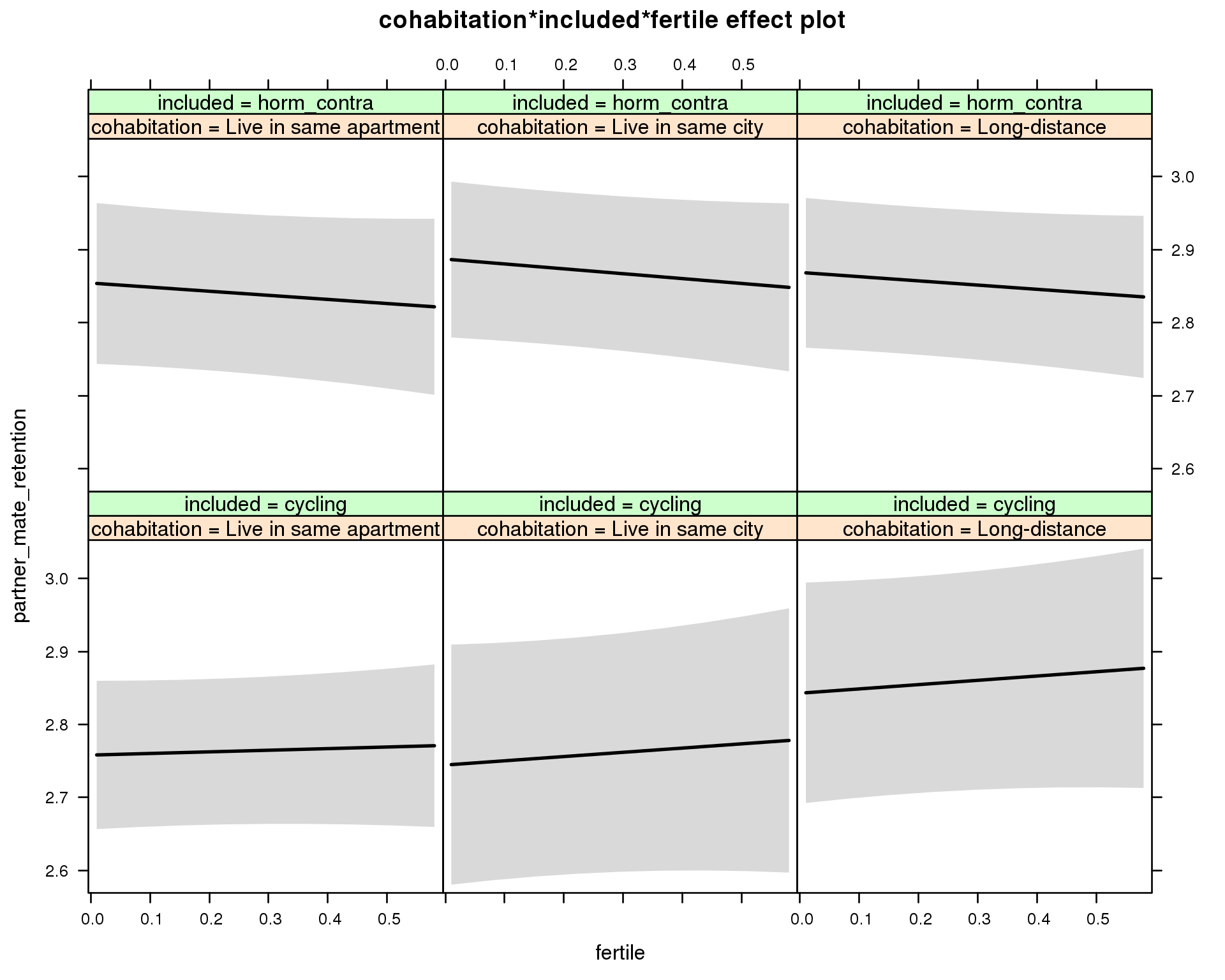
Linear mixed model fit by REML ['lmerMod']
Formula: partner_mate_retention ~ menstruation + fertile_mean + (1 | person) +
cohabitation + included + fertile + menstruation:included +
cohabitation:included + cohabitation:fertile + included:fertile + cohabitation:included:fertile
Data: diary
REML criterion at convergence: 66959
Scaled residuals:
Min 1Q Median 3Q Max
-4.692 -0.609 0.010 0.613 4.869
Random effects:
Groups Name Variance Std.Dev.
person (Intercept) 0.542 0.736
Residual 0.642 0.801
Number of obs: 26680, groups: person, 1054
Fixed effects:
Estimate Std. Error t value
(Intercept) 2.7947 0.0719 38.9
menstruationpre -0.0317 0.0245 -1.3
menstruationyes -0.0601 0.0231 -2.6
fertile_mean -0.1179 0.2873 -0.4
cohabitationLive in same city -0.0136 0.0985 -0.1
cohabitationLong-distance 0.0847 0.0928 0.9
includedhorm_contra 0.0903 0.0776 1.2
fertile 0.0221 0.0617 0.4
menstruationpre:includedhorm_contra 0.0206 0.0314 0.7
menstruationyes:includedhorm_contra 0.0130 0.0302 0.4
cohabitationLive in same city:includedhorm_contra 0.0464 0.1259 0.4
cohabitationLong-distance:includedhorm_contra -0.0702 0.1205 -0.6
cohabitationLive in same city:fertile 0.0359 0.1129 0.3
cohabitationLong-distance:fertile 0.0366 0.1016 0.4
includedhorm_contra:fertile -0.0782 0.0902 -0.9
cohabitationLive in same city:includedhorm_contra:fertile -0.0466 0.1411 -0.3
cohabitationLong-distance:includedhorm_contra:fertile -0.0384 0.1309 -0.3
M_m10: Moderation by relationship status
model %>%
test_moderator("relationship_status_clean", diary)refitting model(s) with ML (instead of REML)
| Df | AIC | BIC | logLik | deviance | Chisq | Chi Df | Pr(>Chisq) | |
|---|---|---|---|---|---|---|---|---|
| with_main | 15 | 66908 | 67031 | -33439 | 66878 | NA | NA | NA |
| with_mod | 19 | 66910 | 67066 | -33436 | 66872 | 6.227 | 4 | 0.1828 |
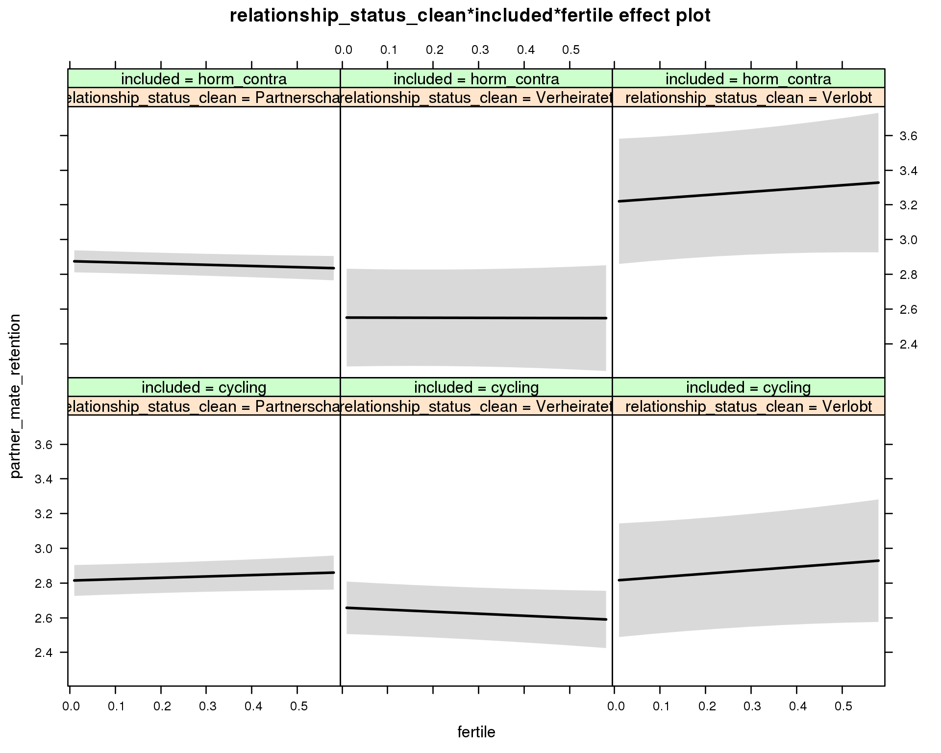
Linear mixed model fit by REML ['lmerMod']
Formula: partner_mate_retention ~ menstruation + fertile_mean + (1 | person) +
relationship_status_clean + included + fertile + menstruation:included +
relationship_status_clean:included + relationship_status_clean:fertile +
included:fertile + relationship_status_clean:included:fertile
Data: diary
REML criterion at convergence: 66931
Scaled residuals:
Min 1Q Median 3Q Max
-4.692 -0.607 0.009 0.613 4.871
Random effects:
Groups Name Variance Std.Dev.
person (Intercept) 0.535 0.731
Residual 0.642 0.801
Number of obs: 26680, groups: person, 1054
Fixed effects:
Estimate Std. Error t value
(Intercept) 2.846330 0.066949 42.5
menstruationpre -0.031389 0.024469 -1.3
menstruationyes -0.059833 0.023061 -2.6
fertile_mean -0.094426 0.285592 -0.3
relationship_status_cleanVerheiratet -0.155586 0.089448 -1.7
relationship_status_cleanVerlobt 0.000372 0.173219 0.0
includedhorm_contra 0.056113 0.057469 1.0
fertile 0.079385 0.056546 1.4
menstruationpre:includedhorm_contra 0.019996 0.031414 0.6
menstruationyes:includedhorm_contra 0.012680 0.030232 0.4
relationship_status_cleanVerheiratet:includedhorm_contra -0.169340 0.172546 -1.0
relationship_status_cleanVerlobt:includedhorm_contra 0.342758 0.255101 1.3
relationship_status_cleanVerheiratet:fertile -0.196991 0.099556 -2.0
relationship_status_cleanVerlobt:fertile 0.117847 0.186727 0.6
includedhorm_contra:fertile -0.148650 0.068949 -2.2
relationship_status_cleanVerheiratet:includedhorm_contra:fertile 0.260757 0.187470 1.4
relationship_status_cleanVerlobt:includedhorm_contra:fertile 0.140249 0.289955 0.5
do_moderators(models$partner_mate_retention, diary)Moderators
Partner’s physical attractiveness
Predicted fertile phase effect sizes (in red): biggest (EP desire, partner mate retention)/smallest (IP desire) when partner’s physical attractiveness is low.
model %>%
test_moderator("partner_attractiveness_physical", diary)refitting model(s) with ML (instead of REML)
| Df | AIC | BIC | logLik | deviance | Chisq | Chi Df | Pr(>Chisq) | |
|---|---|---|---|---|---|---|---|---|
| with_main | 13 | 66883 | 66990 | -33429 | 66857 | NA | NA | NA |
| with_mod | 15 | 66886 | 67009 | -33428 | 66856 | 1.182 | 2 | 0.5538 |
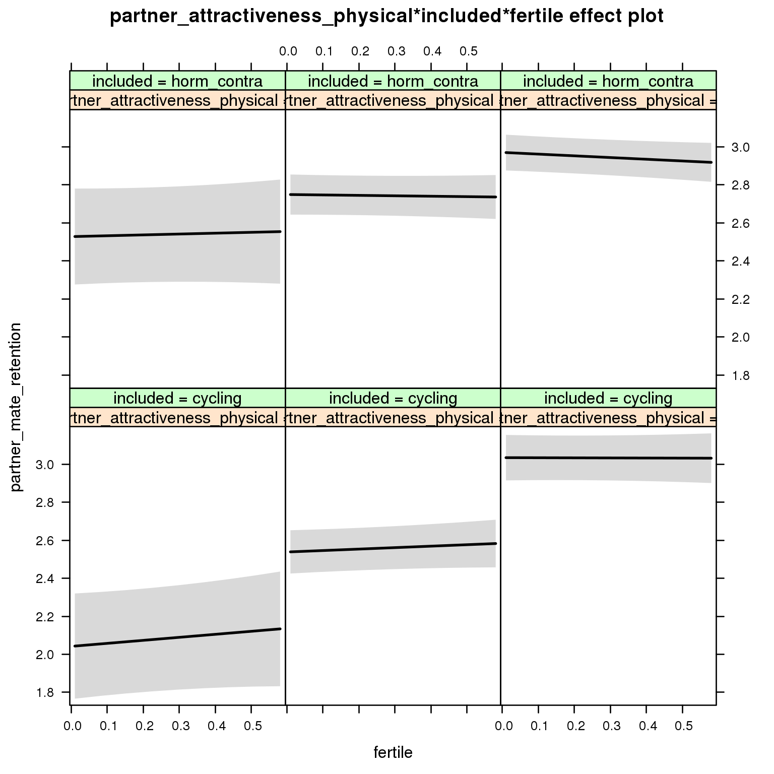
Linear mixed model fit by REML ['lmerMod']
Formula: partner_mate_retention ~ menstruation + fertile_mean + (1 | person) +
partner_attractiveness_physical + included + fertile + menstruation:included +
partner_attractiveness_physical:included + partner_attractiveness_physical:fertile +
included:fertile + partner_attractiveness_physical:included:fertile
Data: diary
REML criterion at convergence: 66923
Scaled residuals:
Min 1Q Median 3Q Max
-4.695 -0.609 0.008 0.612 4.869
Random effects:
Groups Name Variance Std.Dev.
person (Intercept) 0.523 0.723
Residual 0.642 0.801
Number of obs: 26680, groups: person, 1054
Fixed effects:
Estimate Std. Error t value
(Intercept) 1.8341 0.1920 9.55
menstruationpre -0.0327 0.0245 -1.34
menstruationyes -0.0614 0.0231 -2.66
fertile_mean -0.1372 0.2828 -0.49
partner_attractiveness_physical 0.1240 0.0230 5.39
includedhorm_contra 0.6174 0.2514 2.46
fertile 0.1993 0.2156 0.92
menstruationpre:includedhorm_contra 0.0216 0.0314 0.69
menstruationyes:includedhorm_contra 0.0141 0.0302 0.47
partner_attractiveness_physical:includedhorm_contra -0.0687 0.0307 -2.24
partner_attractiveness_physical:fertile -0.0204 0.0264 -0.77
includedhorm_contra:fertile -0.1203 0.2852 -0.42
partner_attractiveness_physical:includedhorm_contra:fertile 0.0035 0.0345 0.10
Partner’s short-term attractiveness
Predicted fertile phase effect sizes (in red): biggest (EP desire, partner mate retention)/smallest (IP desire) when partner’s short-term attractiveness is low.
model %>%
test_moderator("partner_attractiveness_shortterm", diary)refitting model(s) with ML (instead of REML)
| Df | AIC | BIC | logLik | deviance | Chisq | Chi Df | Pr(>Chisq) | |
|---|---|---|---|---|---|---|---|---|
| with_main | 13 | 66890 | 66996 | -33432 | 66864 | NA | NA | NA |
| with_mod | 15 | 66892 | 67015 | -33431 | 66862 | 1.292 | 2 | 0.5242 |
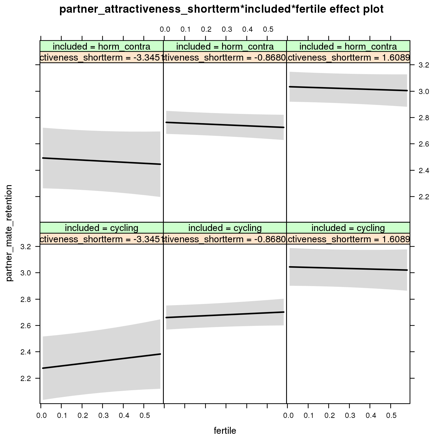
Linear mixed model fit by REML ['lmerMod']
Formula: partner_mate_retention ~ menstruation + fertile_mean + (1 | person) +
partner_attractiveness_shortterm + included + fertile + menstruation:included +
partner_attractiveness_shortterm:included + partner_attractiveness_shortterm:fertile +
included:fertile + partner_attractiveness_shortterm:included:fertile
Data: diary
REML criterion at convergence: 66925
Scaled residuals:
Min 1Q Median 3Q Max
-4.687 -0.608 0.010 0.612 4.872
Random effects:
Groups Name Variance Std.Dev.
person (Intercept) 0.526 0.725
Residual 0.642 0.801
Number of obs: 26680, groups: person, 1054
Fixed effects:
Estimate Std. Error t value
(Intercept) 2.8337 0.0622 45.6
menstruationpre -0.0322 0.0245 -1.3
menstruationyes -0.0611 0.0231 -2.7
fertile_mean -0.1323 0.2834 -0.5
partner_attractiveness_shortterm 0.1557 0.0363 4.3
includedhorm_contra 0.0579 0.0511 1.1
fertile 0.0326 0.0496 0.7
menstruationpre:includedhorm_contra 0.0210 0.0314 0.7
menstruationyes:includedhorm_contra 0.0138 0.0302 0.5
partner_attractiveness_shortterm:includedhorm_contra -0.0465 0.0489 -1.0
partner_attractiveness_shortterm:fertile -0.0465 0.0415 -1.1
includedhorm_contra:fertile -0.0940 0.0629 -1.5
partner_attractiveness_shortterm:includedhorm_contra:fertile 0.0529 0.0544 1.0
Partner’s short-term vs. long-term attractiveness
Predicted fertile phase effect sizes (in red): biggest (EP desire, partner mate retention)/smallest (IP desire) top-right (high LT, low ST), then top-left (low LT, low ST), then bottom-left (low LT, high ST), then bottom-right (high LT/ST).
add_main = update.formula(formula(model), new = as.formula(paste0(". ~ . + partner_attractiveness_longterm * included + partner_attractiveness_shortterm * included + partner_attractiveness_longterm * partner_attractiveness_shortterm"))) # reorder so that the triptych looks nice
add_mod_formula = update.formula(update.formula(formula(model), new = . ~ . - included * fertile), new = as.formula(paste0(". ~ . + partner_attractiveness_longterm * fertile * partner_attractiveness_shortterm * included"))) # reorder so that the triptych looks nice
update(model, formula = add_main) -> with_main
update(model, formula = add_mod_formula) -> with_mod
cat(pander(anova(with_main, with_mod)))refitting model(s) with ML (instead of REML)
| Df | AIC | BIC | logLik | deviance | Chisq | Chi Df | Pr(>Chisq) | |
|---|---|---|---|---|---|---|---|---|
| with_main | 16 | 66872 | 67003 | -33420 | 66840 | NA | NA | NA |
| with_mod | 23 | 66878 | 67066 | -33416 | 66832 | 8.79 | 7 | 0.2681 |
effs = allEffects(with_mod)
effs = data.frame(effs$`partner_attractiveness_longterm:fertile:partner_attractiveness_shortterm:included`) %>%
filter(partner_attractiveness_longterm %in% c(-2,0),partner_attractiveness_shortterm %in% c(-2,0))
ggplot(effs, aes(fertile, fit, ymin = lower, ymax = upper, color = included)) +
facet_grid(partner_attractiveness_shortterm ~ partner_attractiveness_longterm) +
geom_smooth(stat='identity') +
scale_color_manual(values = c("cycling" = 'red', 'horm_contra' = 'black'), guide = F) +
scale_fill_manual(values = c("cycling" = 'red', 'horm_contra' = 'black'), guide = F) +
ggtitle("Moderation", "top-to-bottom: short-term,\nleft-to-right: long-term attractiveness of the partner")+
ylab(names(model@frame)[1])
print_summary(with_mod)Linear mixed model fit by REML ['lmerMod']
Formula: partner_mate_retention ~ menstruation + fertile_mean + (1 | person) +
partner_attractiveness_longterm + fertile + partner_attractiveness_shortterm +
included + menstruation:included + partner_attractiveness_longterm:fertile +
partner_attractiveness_longterm:partner_attractiveness_shortterm +
fertile:partner_attractiveness_shortterm + partner_attractiveness_longterm:included +
fertile:included + partner_attractiveness_shortterm:included +
partner_attractiveness_longterm:fertile:partner_attractiveness_shortterm +
partner_attractiveness_longterm:fertile:included + partner_attractiveness_longterm:partner_attractiveness_shortterm:included +
fertile:partner_attractiveness_shortterm:included + partner_attractiveness_longterm:fertile:partner_attractiveness_shortterm:included
Data: diary
REML criterion at convergence: 66932
Scaled residuals:
Min 1Q Median 3Q Max
-4.686 -0.608 0.008 0.610 4.879
Random effects:
Groups Name Variance Std.Dev.
person (Intercept) 0.515 0.718
Residual 0.642 0.801
Number of obs: 26680, groups: person, 1054
Fixed effects:
Estimate
(Intercept) 2.81701
menstruationpre -0.03219
menstruationyes -0.06046
fertile_mean -0.06556
partner_attractiveness_longterm 0.14712
fertile 0.03687
partner_attractiveness_shortterm 0.09463
includedhorm_contra 0.06543
menstruationpre:includedhorm_contra 0.02161
menstruationyes:includedhorm_contra 0.01370
partner_attractiveness_longterm:fertile 0.02526
partner_attractiveness_longterm:partner_attractiveness_shortterm -0.00182
fertile:partner_attractiveness_shortterm -0.06137
partner_attractiveness_longterm:includedhorm_contra -0.05930
fertile:includedhorm_contra -0.11964
partner_attractiveness_shortterm:includedhorm_contra -0.00456
partner_attractiveness_longterm:fertile:partner_attractiveness_shortterm -0.01637
partner_attractiveness_longterm:fertile:includedhorm_contra 0.03147
partner_attractiveness_longterm:partner_attractiveness_shortterm:includedhorm_contra -0.01948
fertile:partner_attractiveness_shortterm:includedhorm_contra 0.04696
partner_attractiveness_longterm:fertile:partner_attractiveness_shortterm:includedhorm_contra 0.11389
Std. Error
(Intercept) 0.06334
menstruationpre 0.02447
menstruationyes 0.02309
fertile_mean 0.28171
partner_attractiveness_longterm 0.04348
fertile 0.05170
partner_attractiveness_shortterm 0.04005
includedhorm_contra 0.05311
menstruationpre:includedhorm_contra 0.03141
menstruationyes:includedhorm_contra 0.03025
partner_attractiveness_longterm:fertile 0.05000
partner_attractiveness_longterm:partner_attractiveness_shortterm 0.03201
fertile:partner_attractiveness_shortterm 0.04532
partner_attractiveness_longterm:includedhorm_contra 0.05544
fertile:includedhorm_contra 0.06518
partner_attractiveness_shortterm:includedhorm_contra 0.05223
partner_attractiveness_longterm:fertile:partner_attractiveness_shortterm 0.03703
partner_attractiveness_longterm:fertile:includedhorm_contra 0.06340
partner_attractiveness_longterm:partner_attractiveness_shortterm:includedhorm_contra 0.04997
fertile:partner_attractiveness_shortterm:includedhorm_contra 0.05810
partner_attractiveness_longterm:fertile:partner_attractiveness_shortterm:includedhorm_contra 0.05732
t value
(Intercept) 44.5
menstruationpre -1.3
menstruationyes -2.6
fertile_mean -0.2
partner_attractiveness_longterm 3.4
fertile 0.7
partner_attractiveness_shortterm 2.4
includedhorm_contra 1.2
menstruationpre:includedhorm_contra 0.7
menstruationyes:includedhorm_contra 0.5
partner_attractiveness_longterm:fertile 0.5
partner_attractiveness_longterm:partner_attractiveness_shortterm -0.1
fertile:partner_attractiveness_shortterm -1.4
partner_attractiveness_longterm:includedhorm_contra -1.1
fertile:includedhorm_contra -1.8
partner_attractiveness_shortterm:includedhorm_contra -0.1
partner_attractiveness_longterm:fertile:partner_attractiveness_shortterm -0.4
partner_attractiveness_longterm:fertile:includedhorm_contra 0.5
partner_attractiveness_longterm:partner_attractiveness_shortterm:includedhorm_contra -0.4
fertile:partner_attractiveness_shortterm:includedhorm_contra 0.8
partner_attractiveness_longterm:fertile:partner_attractiveness_shortterm:includedhorm_contra 2.0
Relative attractiveness to self
whole MV and MV_P scale
Predicted fertile phase effect sizes (in red): biggest (EP desire, partner mate retention)/smallest (IP desire) when partner’s relative attractiveness is low.
three item subsets of the MV/MV_P scale
model %>%
test_moderator("partner_attractiveness_rel_to_self_MV_short", diary)refitting model(s) with ML (instead of REML)
| Df | AIC | BIC | logLik | deviance | Chisq | Chi Df | Pr(>Chisq) | |
|---|---|---|---|---|---|---|---|---|
| with_main | 13 | 66918 | 67025 | -33446 | 66892 | NA | NA | NA |
| with_mod | 15 | 66919 | 67042 | -33444 | 66889 | 3.412 | 2 | 0.1816 |
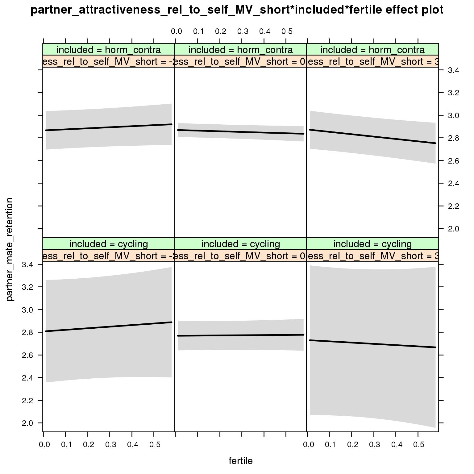
Linear mixed model fit by REML ['lmerMod']
Formula: partner_mate_retention ~ menstruation + fertile_mean + (1 | person) +
partner_attractiveness_rel_to_self_MV_short + included +
fertile + menstruation:included + partner_attractiveness_rel_to_self_MV_short:included +
partner_attractiveness_rel_to_self_MV_short:fertile + included:fertile +
partner_attractiveness_rel_to_self_MV_short:included:fertile
Data: diary
REML criterion at convergence: 66949
Scaled residuals:
Min 1Q Median 3Q Max
-4.693 -0.607 0.010 0.611 4.871
Random effects:
Groups Name Variance Std.Dev.
person (Intercept) 0.541 0.735
Residual 0.642 0.801
Number of obs: 26680, groups: person, 1054
Fixed effects:
Estimate Std. Error t value
(Intercept) 2.80663 0.07058 39.8
menstruationpre -0.03170 0.02447 -1.3
menstruationyes -0.06023 0.02307 -2.6
fertile_mean -0.10641 0.28664 -0.4
partner_attractiveness_rel_to_self_MV_short -0.01224 0.08985 -0.1
includedhorm_contra 0.09171 0.06047 1.5
fertile 0.02484 0.05871 0.4
menstruationpre:includedhorm_contra 0.02096 0.03142 0.7
menstruationyes:includedhorm_contra 0.01388 0.03024 0.5
partner_attractiveness_rel_to_self_MV_short:includedhorm_contra 0.01350 0.09344 0.1
partner_attractiveness_rel_to_self_MV_short:fertile -0.03987 0.09542 -0.4
includedhorm_contra:fertile -0.07027 0.07066 -1.0
partner_attractiveness_rel_to_self_MV_short:includedhorm_contra:fertile -0.00823 0.09910 -0.1
model %>%
test_moderator("partner_attractiveness_rel_to_self", diary)refitting model(s) with ML (instead of REML)
| Df | AIC | BIC | logLik | deviance | Chisq | Chi Df | Pr(>Chisq) | |
|---|---|---|---|---|---|---|---|---|
| with_main | 13 | 66918 | 67024 | -33446 | 66892 | NA | NA | NA |
| with_mod | 15 | 66919 | 67042 | -33444 | 66889 | 2.698 | 2 | 0.2595 |
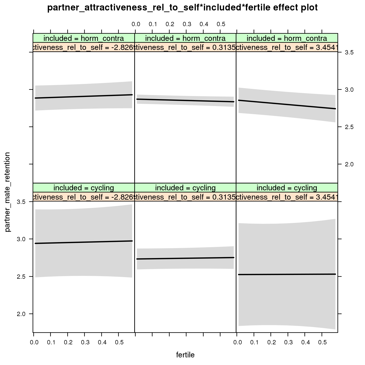
Linear mixed model fit by REML ['lmerMod']
Formula: partner_mate_retention ~ menstruation + fertile_mean + (1 | person) +
partner_attractiveness_rel_to_self + included + fertile +
menstruation:included + partner_attractiveness_rel_to_self:included +
partner_attractiveness_rel_to_self:fertile + included:fertile +
partner_attractiveness_rel_to_self:included:fertile
Data: diary
REML criterion at convergence: 66949
Scaled residuals:
Min 1Q Median 3Q Max
-4.693 -0.608 0.009 0.612 4.872
Random effects:
Groups Name Variance Std.Dev.
person (Intercept) 0.541 0.735
Residual 0.642 0.801
Number of obs: 26680, groups: person, 1054
Fixed effects:
Estimate Std. Error t value
(Intercept) 2.78760 0.07070 39.4
menstruationpre -0.03177 0.02447 -1.3
menstruationyes -0.06020 0.02307 -2.6
fertile_mean -0.10255 0.28659 -0.4
partner_attractiveness_rel_to_self -0.06638 0.09222 -0.7
includedhorm_contra 0.11170 0.06067 1.8
fertile 0.03553 0.05912 0.6
menstruationpre:includedhorm_contra 0.02099 0.03142 0.7
menstruationyes:includedhorm_contra 0.01375 0.03024 0.5
partner_attractiveness_rel_to_self:includedhorm_contra 0.06207 0.09569 0.6
partner_attractiveness_rel_to_self:fertile -0.00756 0.09882 -0.1
includedhorm_contra:fertile -0.08219 0.07102 -1.2
partner_attractiveness_rel_to_self:includedhorm_contra:fertile -0.03630 0.10237 -0.4
Partner’s shortterm attractiveness, alternative specification
model %>%
test_moderator("partner_attractiveness_shortterm_v2", diary)refitting model(s) with ML (instead of REML)
| Df | AIC | BIC | logLik | deviance | Chisq | Chi Df | Pr(>Chisq) | |
|---|---|---|---|---|---|---|---|---|
| with_main | 13 | 66897 | 67003 | -33435 | 66871 | NA | NA | NA |
| with_mod | 15 | 66898 | 67021 | -33434 | 66868 | 2.666 | 2 | 0.2637 |
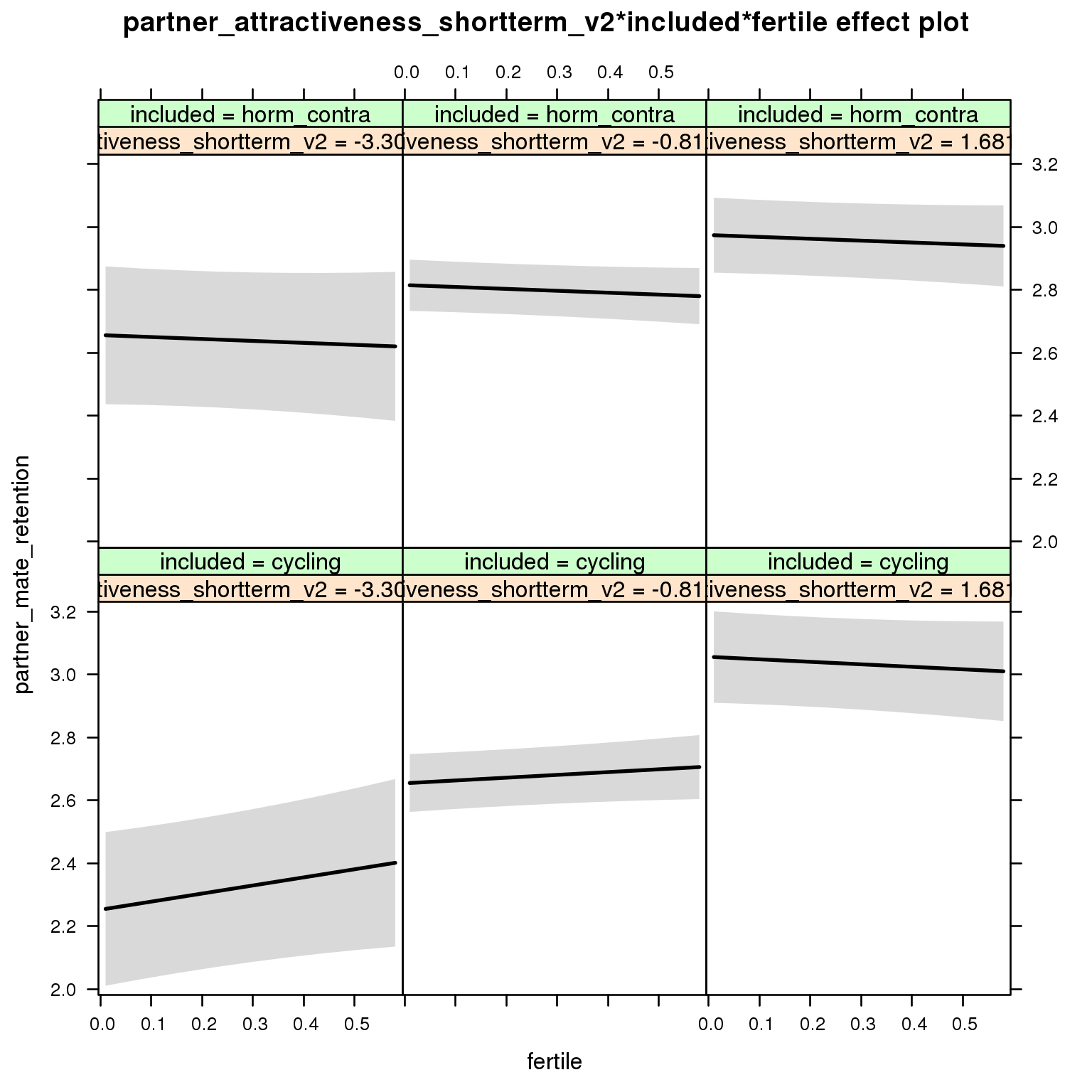
Linear mixed model fit by REML ['lmerMod']
Formula: partner_mate_retention ~ menstruation + fertile_mean + (1 | person) +
partner_attractiveness_shortterm_v2 + included + fertile +
menstruation:included + partner_attractiveness_shortterm_v2:included +
partner_attractiveness_shortterm_v2:fertile + included:fertile +
partner_attractiveness_shortterm_v2:included:fertile
Data: diary
REML criterion at convergence: 66931
Scaled residuals:
Min 1Q Median 3Q Max
-4.694 -0.609 0.010 0.613 4.869
Random effects:
Groups Name Variance Std.Dev.
person (Intercept) 0.530 0.728
Residual 0.642 0.801
Number of obs: 26680, groups: person, 1054
Fixed effects:
Estimate Std. Error t value
(Intercept) 2.8267 0.0623 45.4
menstruationpre -0.0326 0.0245 -1.3
menstruationyes -0.0616 0.0231 -2.7
fertile_mean -0.1409 0.2844 -0.5
partner_attractiveness_shortterm_v2 0.1612 0.0366 4.4
includedhorm_contra 0.0753 0.0511 1.5
fertile 0.0340 0.0494 0.7
menstruationpre:includedhorm_contra 0.0214 0.0314 0.7
menstruationyes:includedhorm_contra 0.0143 0.0302 0.5
partner_attractiveness_shortterm_v2:includedhorm_contra -0.0974 0.0487 -2.0
partner_attractiveness_shortterm_v2:fertile -0.0674 0.0413 -1.6
includedhorm_contra:fertile -0.0943 0.0627 -1.5
partner_attractiveness_shortterm_v2:includedhorm_contra:fertile 0.0679 0.0538 1.3
Partner’s global attractiveness
model %>%
test_moderator("partner_attractiveness_global", diary)refitting model(s) with ML (instead of REML)
| Df | AIC | BIC | logLik | deviance | Chisq | Chi Df | Pr(>Chisq) | |
|---|---|---|---|---|---|---|---|---|
| with_main | 13 | 66913 | 67019 | -33443 | 66887 | NA | NA | NA |
| with_mod | 15 | 66910 | 67033 | -33440 | 66880 | 6.94 | 2 | 0.03112 |
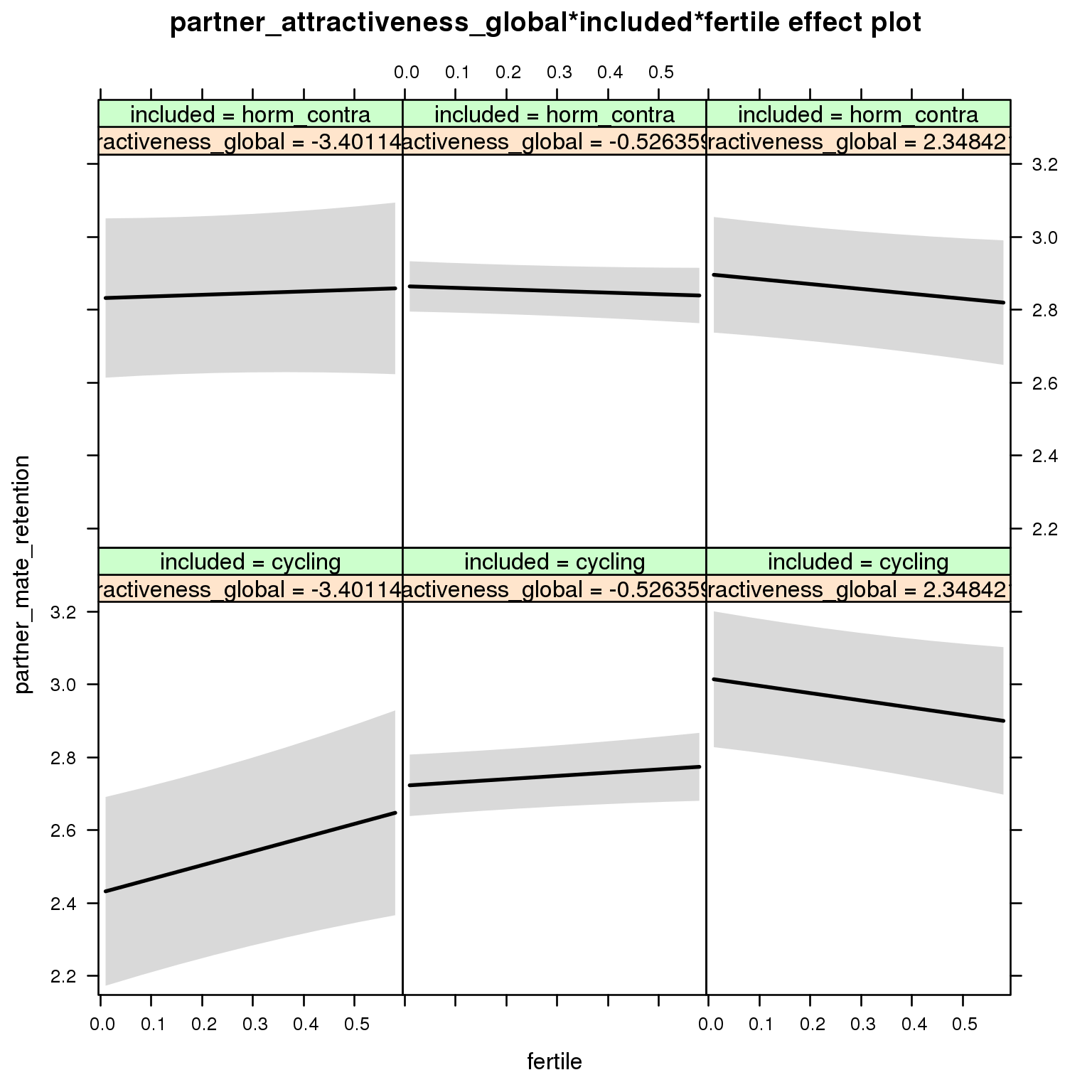
Linear mixed model fit by REML ['lmerMod']
Formula: partner_mate_retention ~ menstruation + fertile_mean + (1 | person) +
partner_attractiveness_global + included + fertile + menstruation:included +
partner_attractiveness_global:included + partner_attractiveness_global:fertile +
included:fertile + partner_attractiveness_global:included:fertile
Data: diary
REML criterion at convergence: 66943
Scaled residuals:
Min 1Q Median 3Q Max
-4.696 -0.609 0.010 0.613 4.873
Random effects:
Groups Name Variance Std.Dev.
person (Intercept) 0.538 0.733
Residual 0.642 0.801
Number of obs: 26680, groups: person, 1054
Fixed effects:
Estimate Std. Error t value
(Intercept) 2.8138 0.0626 45.0
menstruationpre -0.0322 0.0245 -1.3
menstruationyes -0.0607 0.0231 -2.6
fertile_mean -0.1216 0.2861 -0.4
partner_attractiveness_global 0.1023 0.0372 2.7
includedhorm_contra 0.0880 0.0513 1.7
fertile 0.0360 0.0494 0.7
menstruationpre:includedhorm_contra 0.0215 0.0314 0.7
menstruationyes:includedhorm_contra 0.0139 0.0302 0.5
partner_attractiveness_global:includedhorm_contra -0.0909 0.0489 -1.9
partner_attractiveness_global:fertile -0.1006 0.0409 -2.5
includedhorm_contra:fertile -0.0963 0.0626 -1.5
partner_attractiveness_global:includedhorm_contra:fertile 0.0693 0.0526 1.3
Partner’s longterm attractiveness
model %>%
test_moderator("partner_attractiveness_longterm", diary)refitting model(s) with ML (instead of REML)
| Df | AIC | BIC | logLik | deviance | Chisq | Chi Df | Pr(>Chisq) | |
|---|---|---|---|---|---|---|---|---|
| with_main | 13 | 66878 | 66985 | -33426 | 66852 | NA | NA | NA |
| with_mod | 15 | 66880 | 67003 | -33425 | 66850 | 1.892 | 2 | 0.3883 |
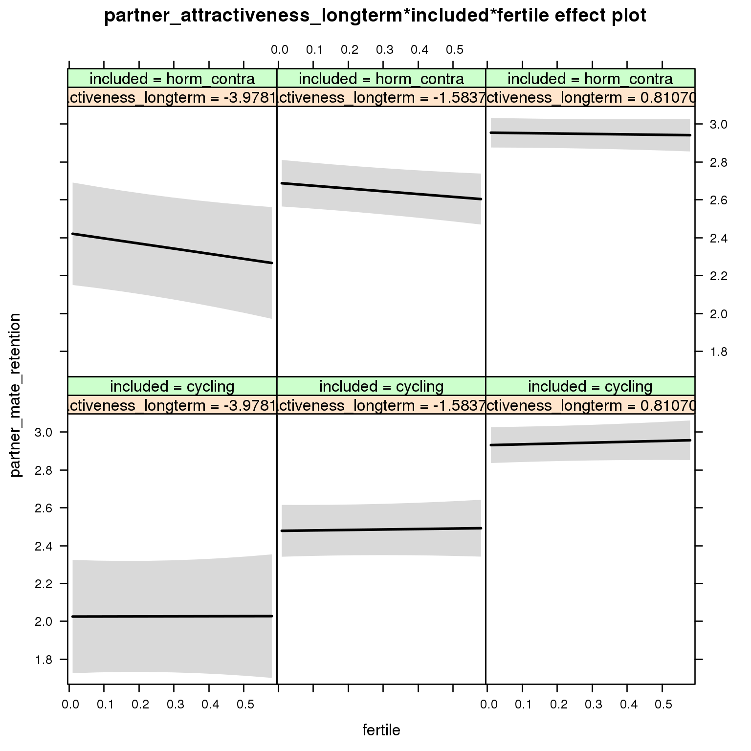
Linear mixed model fit by REML ['lmerMod']
Formula: partner_mate_retention ~ menstruation + fertile_mean + (1 | person) +
partner_attractiveness_longterm + included + fertile + menstruation:included +
partner_attractiveness_longterm:included + partner_attractiveness_longterm:fertile +
included:fertile + partner_attractiveness_longterm:included:fertile
Data: diary
REML criterion at convergence: 66913
Scaled residuals:
Min 1Q Median 3Q Max
-4.688 -0.607 0.011 0.613 4.877
Random effects:
Groups Name Variance Std.Dev.
person (Intercept) 0.519 0.721
Residual 0.642 0.801
Number of obs: 26680, groups: person, 1054
Fixed effects:
Estimate Std. Error t value
(Intercept) 2.8006 0.0617 45.4
menstruationpre -0.0322 0.0245 -1.3
menstruationyes -0.0603 0.0231 -2.6
fertile_mean -0.0399 0.2823 -0.1
partner_attractiveness_longterm 0.1890 0.0373 5.1
includedhorm_contra 0.0817 0.0506 1.6
fertile 0.0378 0.0494 0.8
menstruationpre:includedhorm_contra 0.0214 0.0314 0.7
menstruationyes:includedhorm_contra 0.0138 0.0302 0.5
partner_attractiveness_longterm:includedhorm_contra -0.0780 0.0501 -1.6
partner_attractiveness_longterm:fertile 0.0085 0.0438 0.2
includedhorm_contra:fertile -0.1027 0.0627 -1.6
partner_attractiveness_longterm:includedhorm_contra:fertile 0.0431 0.0579 0.7
Partner’s short-term vs. long-term attractiveness
We also test this specification of the short-term vs. long-term moderator prediction, but we think this is a suboptimal way to test it.
model %>%
test_moderator("partner_st_vs_lt", diary)refitting model(s) with ML (instead of REML)
| Df | AIC | BIC | logLik | deviance | Chisq | Chi Df | Pr(>Chisq) | |
|---|---|---|---|---|---|---|---|---|
| with_main | 13 | 66918 | 67024 | -33446 | 66892 | NA | NA | NA |
| with_mod | 15 | 66919 | 67042 | -33445 | 66889 | 2.347 | 2 | 0.3093 |
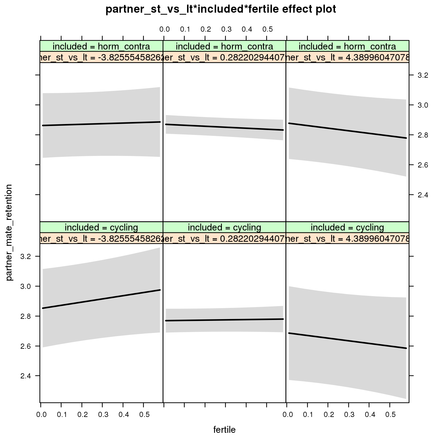
Linear mixed model fit by REML ['lmerMod']
Formula: partner_mate_retention ~ menstruation + fertile_mean + (1 | person) +
partner_st_vs_lt + included + fertile + menstruation:included +
partner_st_vs_lt:included + partner_st_vs_lt:fertile + included:fertile +
partner_st_vs_lt:included:fertile
Data: diary
REML criterion at convergence: 66953
Scaled residuals:
Min 1Q Median 3Q Max
-4.691 -0.608 0.010 0.612 4.870
Random effects:
Groups Name Variance Std.Dev.
person (Intercept) 0.540 0.735
Residual 0.642 0.801
Number of obs: 26680, groups: person, 1054
Fixed effects:
Estimate Std. Error t value
(Intercept) 2.8061 0.0630 44.5
menstruationpre -0.0315 0.0245 -1.3
menstruationyes -0.0594 0.0231 -2.6
fertile_mean -0.0895 0.2869 -0.3
partner_st_vs_lt -0.0198 0.0346 -0.6
includedhorm_contra 0.0898 0.0516 1.7
fertile 0.0317 0.0497 0.6
menstruationpre:includedhorm_contra 0.0206 0.0314 0.7
menstruationyes:includedhorm_contra 0.0126 0.0302 0.4
partner_st_vs_lt:includedhorm_contra 0.0219 0.0441 0.5
partner_st_vs_lt:fertile -0.0476 0.0383 -1.2
includedhorm_contra:fertile -0.0904 0.0628 -1.4
partner_st_vs_lt:includedhorm_contra:fertile 0.0215 0.0482 0.4
Partner’s mate value
long scale
model %>%
test_moderator("MV_P", diary)refitting model(s) with ML (instead of REML)
| Df | AIC | BIC | logLik | deviance | Chisq | Chi Df | Pr(>Chisq) | |
|---|---|---|---|---|---|---|---|---|
| with_main | 13 | 66915 | 67022 | -33445 | 66889 | NA | NA | NA |
| with_mod | 15 | 66912 | 67034 | -33441 | 66882 | 7.511 | 2 | 0.02339 |
Error: Error in plot.eff(x[[(i - 1) * cols + j]], row = i, col = j, nrow = rows, : x.var = ‘fertile’ is not in the effect.
short scale
model %>%
test_moderator("MV_P_short", diary)refitting model(s) with ML (instead of REML)
| Df | AIC | BIC | logLik | deviance | Chisq | Chi Df | Pr(>Chisq) | |
|---|---|---|---|---|---|---|---|---|
| with_main | 13 | 66897 | 67003 | -33435 | 66871 | NA | NA | NA |
| with_mod | 15 | 66894 | 67017 | -33432 | 66864 | 6.346 | 2 | 0.04187 |
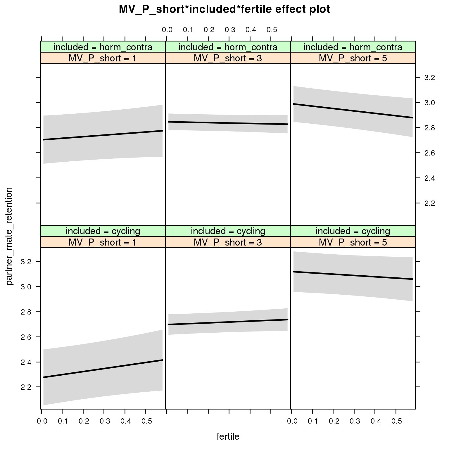
Linear mixed model fit by REML ['lmerMod']
Formula: partner_mate_retention ~ menstruation + fertile_mean + (1 | person) +
MV_P_short + included + fertile + menstruation:included +
MV_P_short:included + MV_P_short:fertile + included:fertile + MV_P_short:included:fertile
Data: diary
REML criterion at convergence: 66926
Scaled residuals:
Min 1Q Median 3Q Max
-4.695 -0.608 0.010 0.611 4.874
Random effects:
Groups Name Variance Std.Dev.
person (Intercept) 0.529 0.727
Residual 0.642 0.801
Number of obs: 26680, groups: person, 1054
Fixed effects:
Estimate Std. Error t value
(Intercept) 2.10205 0.16405 12.81
menstruationpre -0.03260 0.02447 -1.33
menstruationyes -0.06075 0.02306 -2.63
fertile_mean -0.12751 0.28407 -0.45
MV_P_short 0.21114 0.04514 4.68
includedhorm_contra 0.56096 0.20816 2.69
fertile 0.32738 0.17872 1.83
menstruationpre:includedhorm_contra 0.02188 0.03141 0.70
menstruationyes:includedhorm_contra 0.01379 0.03023 0.46
MV_P_short:includedhorm_contra -0.13928 0.06011 -2.32
MV_P_short:fertile -0.08623 0.05111 -1.69
includedhorm_contra:fertile -0.12398 0.23089 -0.54
MV_P_short:includedhorm_contra:fertile 0.00723 0.06632 0.11
Partner’s job and income
model %>%
test_moderator("partner_attractiveness_money", diary)refitting model(s) with ML (instead of REML)
| Df | AIC | BIC | logLik | deviance | Chisq | Chi Df | Pr(>Chisq) | |
|---|---|---|---|---|---|---|---|---|
| with_main | 13 | 66917 | 67024 | -33446 | 66891 | NA | NA | NA |
| with_mod | 15 | 66921 | 67044 | -33446 | 66891 | 0.1106 | 2 | 0.9462 |
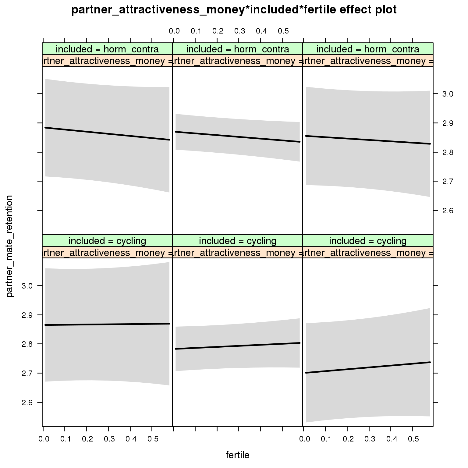
Linear mixed model fit by REML ['lmerMod']
Formula: partner_mate_retention ~ menstruation + fertile_mean + (1 | person) +
partner_attractiveness_money + included + fertile + menstruation:included +
partner_attractiveness_money:included + partner_attractiveness_money:fertile +
included:fertile + partner_attractiveness_money:included:fertile
Data: diary
REML criterion at convergence: 66953
Scaled residuals:
Min 1Q Median 3Q Max
-4.692 -0.609 0.010 0.613 4.870
Random effects:
Groups Name Variance Std.Dev.
person (Intercept) 0.541 0.735
Residual 0.642 0.801
Number of obs: 26680, groups: person, 1054
Fixed effects:
Estimate Std. Error t value
(Intercept) 2.94154 0.14894 19.75
menstruationpre -0.03167 0.02447 -1.29
menstruationyes -0.06014 0.02307 -2.61
fertile_mean -0.11011 0.28675 -0.38
partner_attractiveness_money -0.04116 0.04244 -0.97
includedhorm_contra -0.02048 0.18685 -0.11
fertile -0.00651 0.15712 -0.04
menstruationpre:includedhorm_contra 0.02067 0.03142 0.66
menstruationyes:includedhorm_contra 0.01318 0.03024 0.44
partner_attractiveness_money:includedhorm_contra 0.03399 0.05830 0.58
partner_attractiveness_money:fertile 0.01402 0.04702 0.30
includedhorm_contra:fertile -0.07265 0.20621 -0.35
partner_attractiveness_money:includedhorm_contra:fertile -0.00766 0.06371 -0.12
Female mate retention
model_summaries$female_mate_retentionModel summary
Model summary
model %>%
print_summary()Linear mixed model fit by REML
t-tests use Satterthwaite approximations to degrees of freedom ['lmerMod']
Formula: female_mate_retention ~ included * (menstruation + fertile) + fertile_mean + (1 | person)
Data: diary
REML criterion at convergence: 69606
Scaled residuals:
Min 1Q Median 3Q Max
-4.149 -0.628 -0.003 0.632 4.538
Random effects:
Groups Name Variance Std.Dev.
person (Intercept) 0.543 0.737
Residual 0.712 0.844
Number of obs: 26681, groups: person, 1054
Fixed effects:
Estimate Std. Error df t value Pr(>|t|)
(Intercept) 3.03589 0.06345 1370.00000 47.84 < 2e-16 ***
includedhorm_contra 0.17218 0.05200 1324.00000 3.31 0.00095 ***
menstruationpre -0.00848 0.02576 25959.00000 -0.33 0.74204
menstruationyes 0.01769 0.02428 26062.00000 0.73 0.46612
fertile 0.04253 0.05199 25947.00000 0.82 0.41331
fertile_mean -0.12941 0.29040 1488.00000 -0.45 0.65593
includedhorm_contra:menstruationpre -0.03353 0.03307 25955.00000 -1.01 0.31065
includedhorm_contra:menstruationyes -0.02308 0.03183 26041.00000 -0.73 0.46828
includedhorm_contra:fertile -0.20564 0.06588 26066.00000 -3.12 0.00180 **
---
Signif. codes: 0 '***' 0.001 '**' 0.01 '*' 0.05 '.' 0.1 ' ' 1
Correlation of Fixed Effects:
(Intr) incld_ mnstrtnp mnstrtny fertil frtl_m inclddhrm_cntr:mnstrtnp
inclddhrm_c -0.474
menstrutnpr -0.156 0.198
menstrutnys -0.152 0.191 0.397
fertile -0.150 0.245 0.467 0.385
fertile_men -0.772 -0.025 -0.008 -0.005 -0.064
inclddhrm_cntr:mnstrtnp 0.129 -0.248 -0.779 -0.310 -0.363 -0.003
inclddhrm_cntr:mnstrtny 0.122 -0.234 -0.303 -0.763 -0.293 -0.003 0.383
inclddhrm_cntr:f 0.150 -0.309 -0.368 -0.303 -0.787 0.010 0.467
inclddhrm_cntr:mnstrtny
inclddhrm_c
menstrutnpr
menstrutnys
fertile
fertile_men
inclddhrm_cntr:mnstrtnp
inclddhrm_cntr:mnstrtny
inclddhrm_cntr:f 0.381
Effect size standardised by residual variance (\(\frac{b}{ SD_{residual} }\)): 0.05 [-0.07;0.17].
Marginal effect plots
model %>%
plot_all_effects()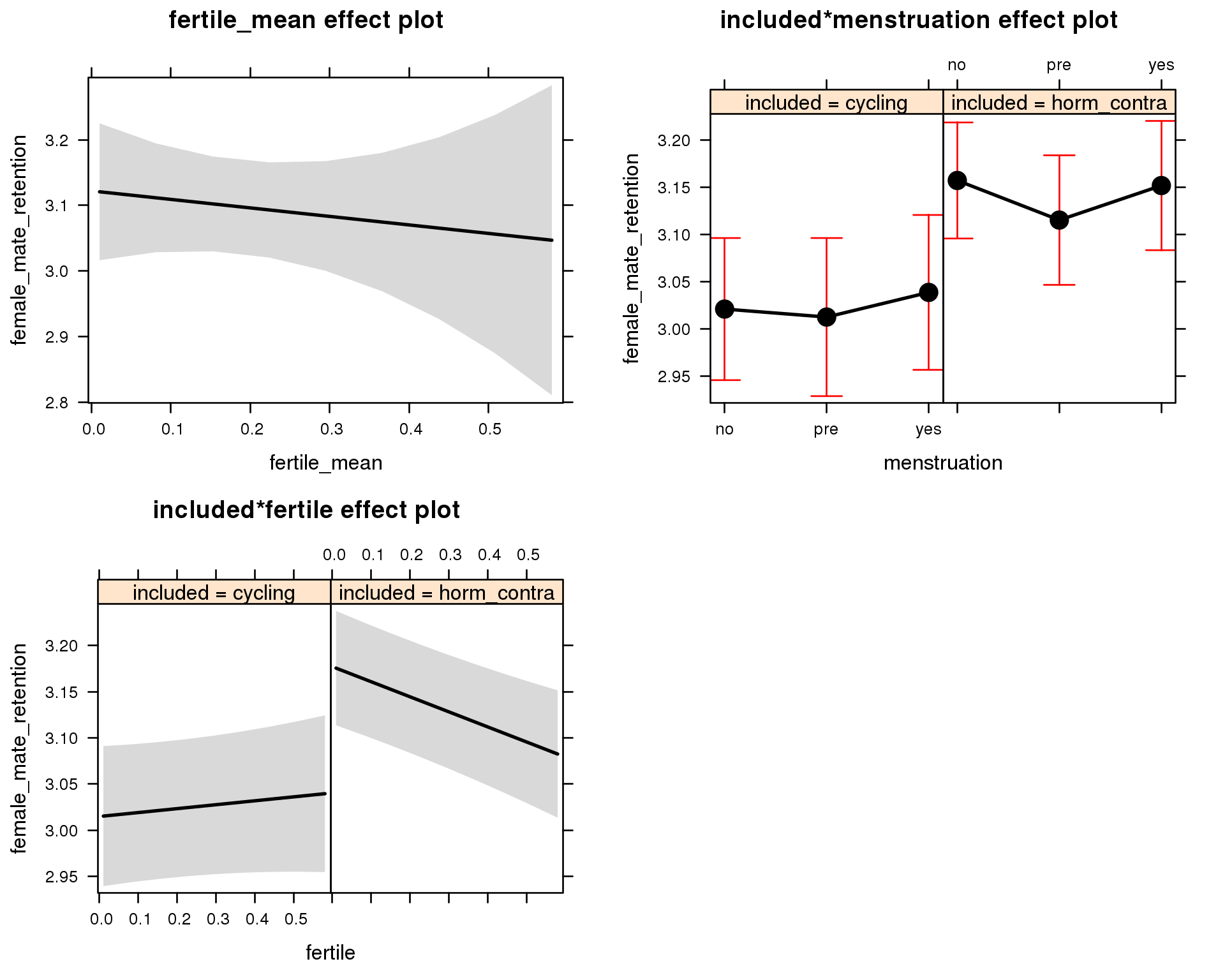
Outcome distribution
model %>%
plot_outcome(diary) + xlab(outcome_label)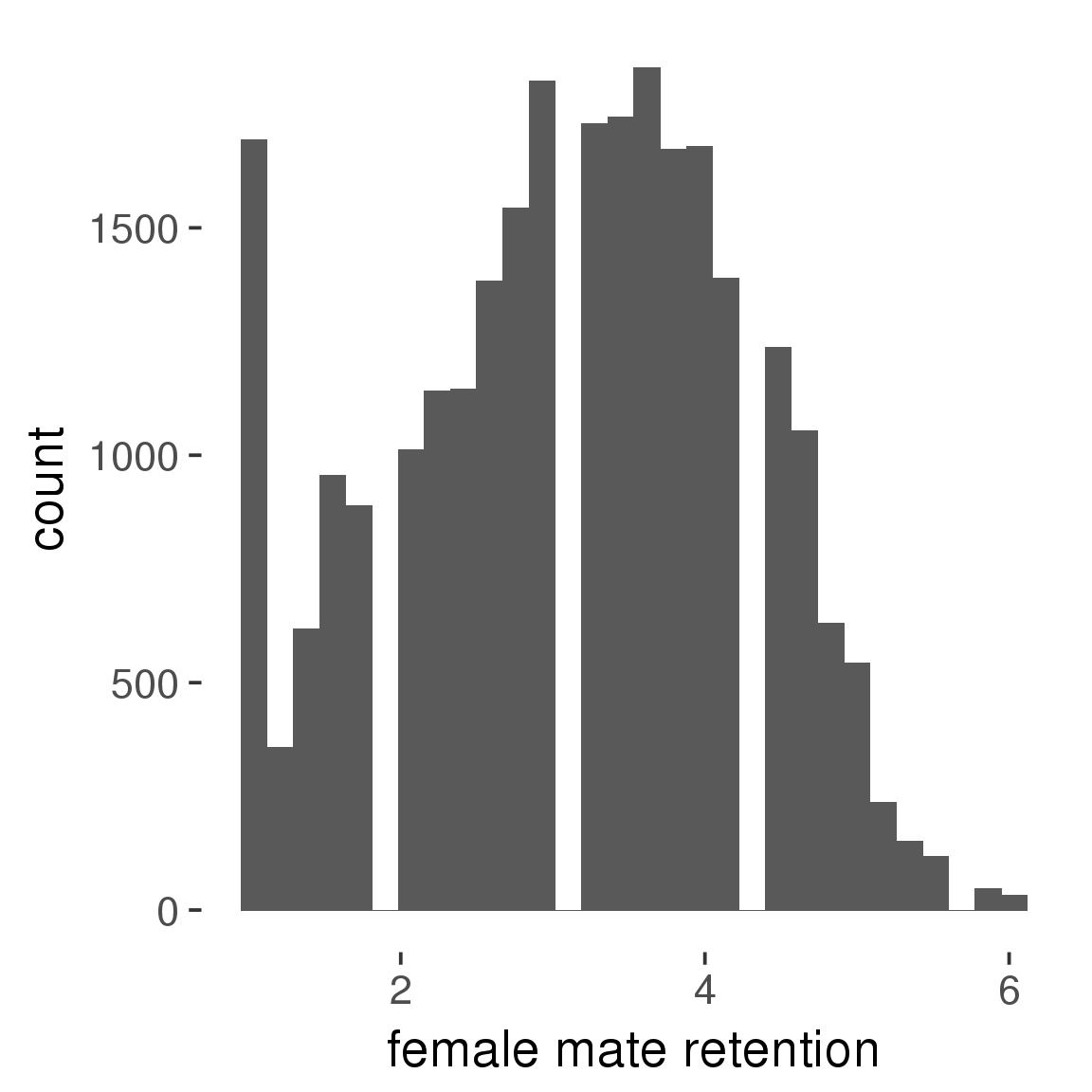
Diagnostics
model %>%
print_diagnostics()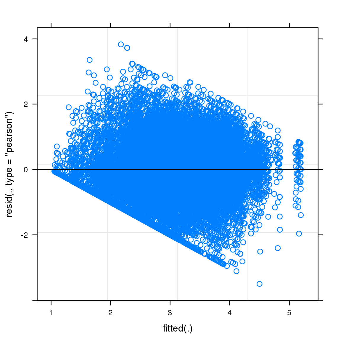


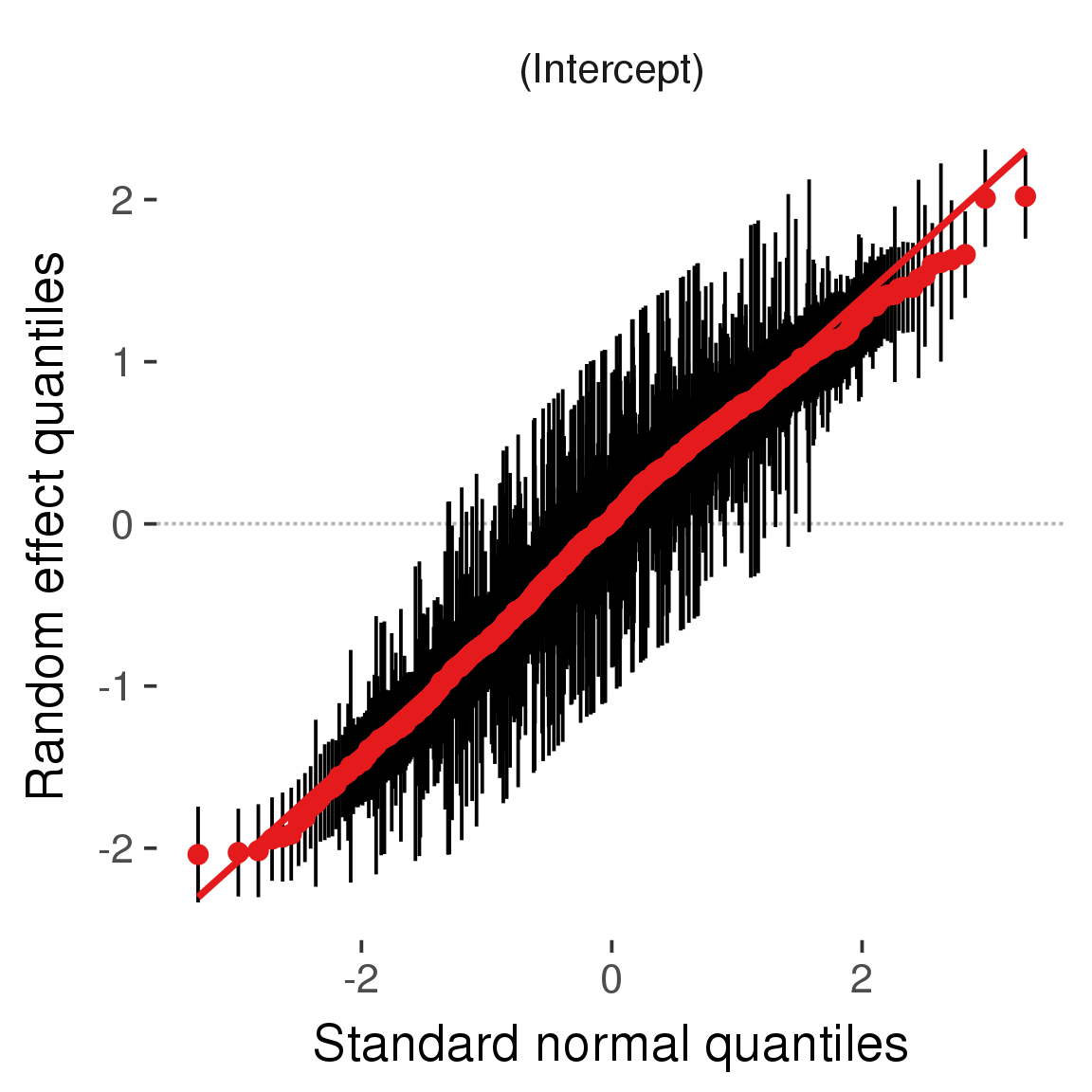
Curves
Here, we continuously plot the outcome over the course of the cycle. Because cycle lengths vary, we subset the data to cycles in a certain range. If the red curve traces the pink curve, our predictor accurately maps the relationship between fertile window probability and the outcome.
Cycle lengths from 21 to 36
Backward-counted
model %>%
plot_curve(diary %>% filter(minimum_cycle_length_diary <= 36, minimum_cycle_length_diary > 20) %>% mutate(fertile=prc_stirn_b))outcome = names(model@frame)[1]
outcome_label = recode(str_replace_all(str_replace_all(str_replace_all(outcome, "_", " "), " pair", "-pair"), " 1", ""),
"desirability 1" = "self-perceived desirability",
"NARQ admiration" = "narcissistic admiration",
"NARQ rivalry" = "narcissistic rivalry",
"extra-pair" = "extra-pair desire & behaviour",
"had sexual intercourse" = "sexual intercourse")
library(ggplot2)
# form a subset and run the model without the hormonal contraception and the fertility predictors
tmp = diary %>%
filter(!is.na(fertile), !is.na(included),
RCD > -1 * minimum_cycle_length_diary, RCD > -40)
new_form = update.formula(formula(model), new = . ~ . - fertile * included)
tmp$residuals = residuals(update(model, new_form, data = tmp , na.action = na.exclude))
tmp = tmp %>%
filter(!is.na(RCD), !is.na(residuals))
rcd_min = min(tmp$RCD)
tmp$real = FALSE
tmp_before = tmp
tmp_before$RCD = tmp_before$RCD + min(tmp$RCD) - 1
tmp_after = tmp
tmp_after$RCD = tmp_after$RCD - min(tmp$RCD) + 1
tmp$real = TRUE
tmp = bind_rows(tmp_before %>% filter(RCD > rcd_min - 11), tmp, tmp_after %>% filter(RCD < 11))GAM smooth on residuals
Here, we partialled out menstruation and individual random effects, then superimposed estimated probability of being in the fertile window scaled to the range of the estimated means. To address the periodicity of the cycle, we prepended and appended ten days of the timeseries to the end and the beginning of the timeseries. We then estimated the GAM and cut off the appended subsets before plotting.
tryCatch({
trend_plot = ggplot(tmp,aes(x = RCD, y = residuals, colour = included)) +
stat_smooth(geom = 'smooth',size = 0.8, fill = "#9ECAE1", method = 'gam', formula = y ~ s(x))
}, error = function(e){cat_message(e, "danger")})
tryCatch({
trend_data = ggplot_build(trend_plot)$data[[1]]
}, error = function(e){cat_message(e, "danger")})
trend_data$RCD = round(trend_data$x)
trend_data = left_join(trend_data, tmp %>% select(real, RCD,fertile) %>% unique(), by = "RCD")
trend_data %>%
filter(real == TRUE) %>%
mutate(superimposed = ( ( (fertile - 0.01)/0.58) * (max(y)-min(y) ) ) + min(y) ) ->
trend_data
ggplot(trend_data) +
geom_ribbon(aes(x = x, ymin = ymin, ymax = ymax, fill = factor(group)), alpha = 0.2) +
geom_line(aes(x = x, y = y, colour = factor(group)), size = 0.8, stat = "identity") +
scale_x_continuous(caption_x) +
geom_line(aes(x = x, y = superimposed), color = "#a83fbf", size = 1, linetype = 'dashed') +
annotate("text",x = mean(trend_data$x), y = max(trend_data$superimposed,na.rm=T) + 0.1, label = 'superimposed fertility peak', color = "#a83fbf") +
scale_y_continuous(outcome_label) +
ggtitle("GAM smooth, residuals") +
scale_color_manual("Contraception status",values = c("2"="black","1"= "red"), labels = c("2"="hormonally\ncontracepting","1"="cycling"), guide = F) +
scale_fill_manual("Contraception status",values = c("2"="black","1"= "red"), labels = c("2"="hormonally\ncontracepting","1"="cycling"), guide = F)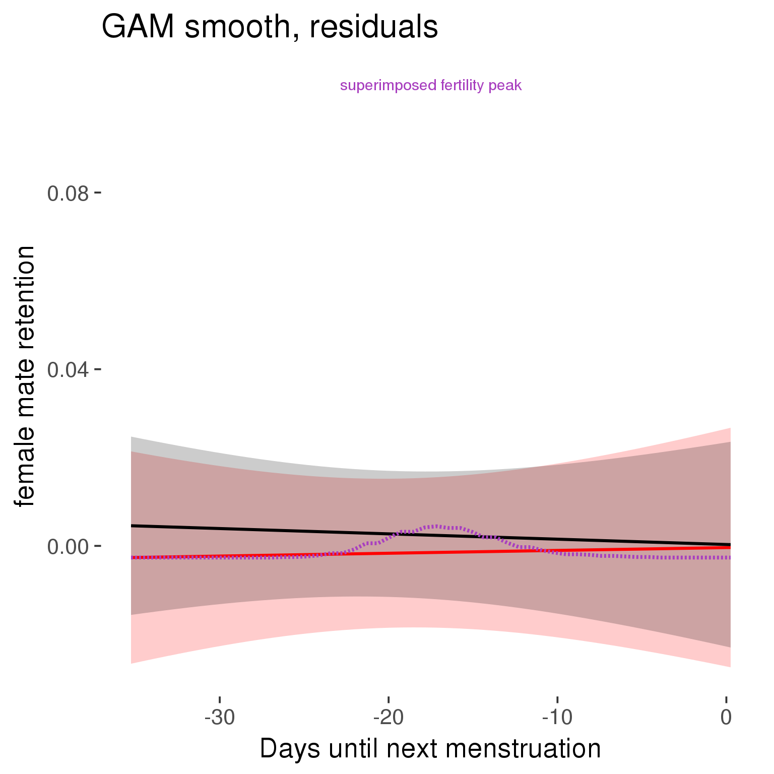
GAM smooth on raw data
As before, but without partialling anything out.
tryCatch({
trend_plot = ggplot(tmp,aes_string(x = "RCD", y = outcome, colour = "included")) +
stat_smooth(geom = 'smooth',size = 0.8, fill = "#9ECAE1", method = 'gam', formula = y ~ s(x))
}, error = function(e){cat_message(e, "danger")})
tryCatch({
trend_data = ggplot_build(trend_plot)$data[[1]]
}, error = function(e){cat_message(e, "danger")})
trend_data$RCD = round(trend_data$x)
trend_data = left_join(trend_data, tmp %>% select(real, RCD,fertile) %>% unique(), by = "RCD")
trend_data %>%
filter(real == TRUE) %>%
mutate(superimposed = ( ( (fertile - 0.01)/0.58) * (max(y)-min(y) ) ) + min(y) ) ->
trend_data
plot1b = ggplot(trend_data) +
geom_ribbon(aes(x = x, ymin = ymin, ymax = ymax, fill = factor(group)), alpha = 0.2) +
geom_line(aes(x = x, y = y, colour = factor(group)), size = 0.8, stat = "identity") +
scale_x_continuous(caption_x) +
geom_line(aes(x = x, y = superimposed), color = "#a83fbf", size = 1, linetype = 'dashed') +
annotate("text",x = mean(trend_data$x), y = max(trend_data$superimposed,na.rm=T) + 0.1, label = 'superimposed fertility peak', color = "#a83fbf") +
scale_y_continuous(outcome_label) +
ggtitle("GAM smooth, raw data") +
scale_color_manual("Contraception status",values = c("2"="black","1"= "red"), labels = c("2"="hormonally\ncontracepting","1"="cycling"), guide = F) +
scale_fill_manual("Contraception status",values = c("2"="black","1"= "red"), labels = c("2"="hormonally\ncontracepting","1"="cycling"), guide = F)
suppressWarnings(print(plot1b))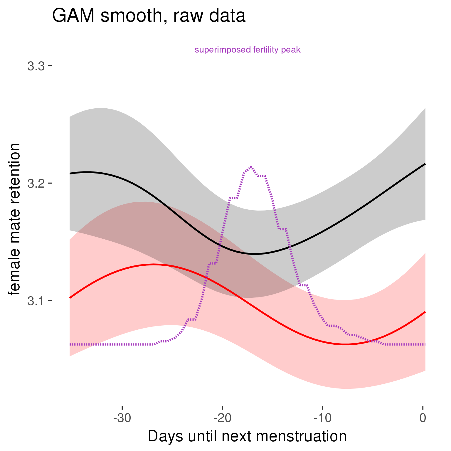
Means and standard errors over raw data
Nothing partialled out, just straight means with bootstrapped confidence intervals.
tryCatch({
trend_plot = ggplot(tmp,aes_string(x = "RCD", y = outcome, colour = "included")) +
geom_pointrange(size = 0.8, stat = 'summary', fun.data = "mean_cl_boot")
}, error = function(e){cat_message(e, "danger")})
tryCatch({
trend_data = ggplot_build(trend_plot)$data[[1]]
}, error = function(e){cat_message(e, "danger")})
trend_data$RCD = round(trend_data$x)
trend_data = left_join(trend_data, tmp %>% select(real, RCD,fertile) %>% unique(), by = "RCD")
trend_data %>%
filter(real == TRUE) %>%
mutate(superimposed = ( ( (fertile - 0.01)/0.58) * (max(y)-min(y) ) ) + min(y) ) ->
trend_data
plot3 = ggplot(trend_data) +
geom_pointrange(aes(x = x, y = y, ymin = ymin,ymax = ymax, colour = factor(group)), size = 0.8, stat = "identity", alpha = 0.6, position = position_dodge(width = .5)) +
scale_x_continuous("Days until next menstruation") +
geom_line(aes(x= x, y = superimposed), color = "#a83fbf", size = 1, linetype = 'dashed') +
annotate("text",x = mean(trend_data$x), y = max(trend_data$superimposed,na.rm=T) + 0.1, label = 'superimposed fertility peak', color = "#a83fbf") +
scale_y_continuous(outcome_label) +
ggtitle("Means with standard errors, raw data") +
scale_color_manual("Contraception status",values = c("2"="black","1"= "red"), labels = c("2"="hormonally\ncontracepting","1"="cycling"), guide = F) +
scale_fill_manual("Contraception status",values = c("2"="black","1"= "red"), labels = c("2"="hormonally\ncontracepting","1"="cycling"), guide = F)
suppressWarnings(print(plot3))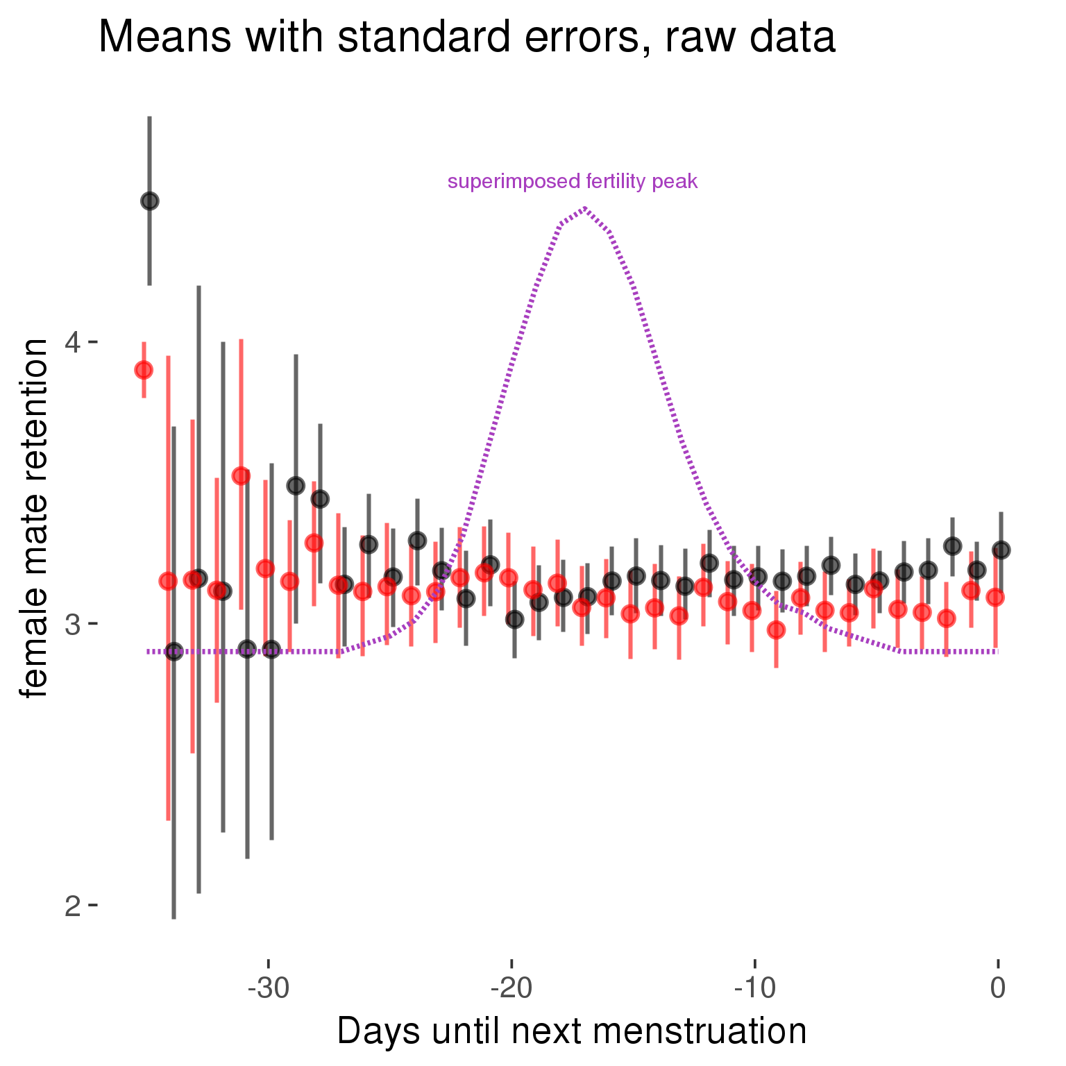
Forward-counted
model %>%
plot_curve(diary %>% filter(minimum_cycle_length_diary <= 36, minimum_cycle_length_diary > 20) %>% mutate(RCD = FCD, fertile = prc_stirn_b_forward_counted), caption_x = "Days since last menstruation")outcome = names(model@frame)[1]
outcome_label = recode(str_replace_all(str_replace_all(str_replace_all(outcome, "_", " "), " pair", "-pair"), " 1", ""),
"desirability 1" = "self-perceived desirability",
"NARQ admiration" = "narcissistic admiration",
"NARQ rivalry" = "narcissistic rivalry",
"extra-pair" = "extra-pair desire & behaviour",
"had sexual intercourse" = "sexual intercourse")
library(ggplot2)
# form a subset and run the model without the hormonal contraception and the fertility predictors
tmp = diary %>%
filter(!is.na(fertile), !is.na(included),
RCD > -1 * minimum_cycle_length_diary, RCD > -40)
new_form = update.formula(formula(model), new = . ~ . - fertile * included)
tmp$residuals = residuals(update(model, new_form, data = tmp , na.action = na.exclude))
tmp = tmp %>%
filter(!is.na(RCD), !is.na(residuals))
rcd_min = min(tmp$RCD)
tmp$real = FALSE
tmp_before = tmp
tmp_before$RCD = tmp_before$RCD + min(tmp$RCD) - 1
tmp_after = tmp
tmp_after$RCD = tmp_after$RCD - min(tmp$RCD) + 1
tmp$real = TRUE
tmp = bind_rows(tmp_before %>% filter(RCD > rcd_min - 11), tmp, tmp_after %>% filter(RCD < 11))GAM smooth on residuals
Here, we partialled out menstruation and individual random effects, then superimposed estimated probability of being in the fertile window scaled to the range of the estimated means. To address the periodicity of the cycle, we prepended and appended ten days of the timeseries to the end and the beginning of the timeseries. We then estimated the GAM and cut off the appended subsets before plotting.
tryCatch({
trend_plot = ggplot(tmp,aes(x = RCD, y = residuals, colour = included)) +
stat_smooth(geom = 'smooth',size = 0.8, fill = "#9ECAE1", method = 'gam', formula = y ~ s(x))
}, error = function(e){cat_message(e, "danger")})
tryCatch({
trend_data = ggplot_build(trend_plot)$data[[1]]
}, error = function(e){cat_message(e, "danger")})
trend_data$RCD = round(trend_data$x)
trend_data = left_join(trend_data, tmp %>% select(real, RCD,fertile) %>% unique(), by = "RCD")
trend_data %>%
filter(real == TRUE) %>%
mutate(superimposed = ( ( (fertile - 0.01)/0.58) * (max(y)-min(y) ) ) + min(y) ) ->
trend_data
ggplot(trend_data) +
geom_ribbon(aes(x = x, ymin = ymin, ymax = ymax, fill = factor(group)), alpha = 0.2) +
geom_line(aes(x = x, y = y, colour = factor(group)), size = 0.8, stat = "identity") +
scale_x_continuous(caption_x) +
geom_line(aes(x = x, y = superimposed), color = "#a83fbf", size = 1, linetype = 'dashed') +
annotate("text",x = mean(trend_data$x), y = max(trend_data$superimposed,na.rm=T) + 0.1, label = 'superimposed fertility peak', color = "#a83fbf") +
scale_y_continuous(outcome_label) +
ggtitle("GAM smooth, residuals") +
scale_color_manual("Contraception status",values = c("2"="black","1"= "red"), labels = c("2"="hormonally\ncontracepting","1"="cycling"), guide = F) +
scale_fill_manual("Contraception status",values = c("2"="black","1"= "red"), labels = c("2"="hormonally\ncontracepting","1"="cycling"), guide = F)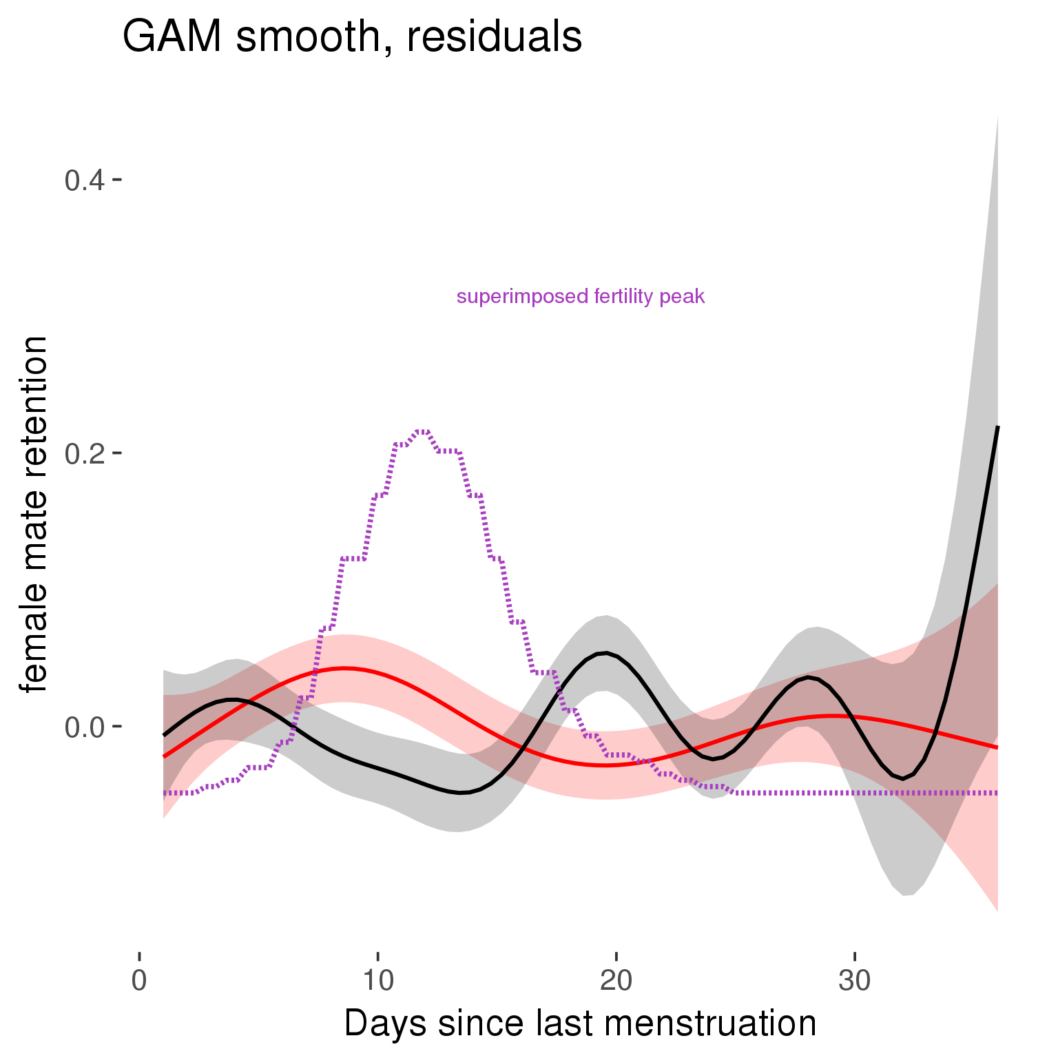
GAM smooth on raw data
As before, but without partialling anything out.
tryCatch({
trend_plot = ggplot(tmp,aes_string(x = "RCD", y = outcome, colour = "included")) +
stat_smooth(geom = 'smooth',size = 0.8, fill = "#9ECAE1", method = 'gam', formula = y ~ s(x))
}, error = function(e){cat_message(e, "danger")})
tryCatch({
trend_data = ggplot_build(trend_plot)$data[[1]]
}, error = function(e){cat_message(e, "danger")})
trend_data$RCD = round(trend_data$x)
trend_data = left_join(trend_data, tmp %>% select(real, RCD,fertile) %>% unique(), by = "RCD")
trend_data %>%
filter(real == TRUE) %>%
mutate(superimposed = ( ( (fertile - 0.01)/0.58) * (max(y)-min(y) ) ) + min(y) ) ->
trend_data
plot1b = ggplot(trend_data) +
geom_ribbon(aes(x = x, ymin = ymin, ymax = ymax, fill = factor(group)), alpha = 0.2) +
geom_line(aes(x = x, y = y, colour = factor(group)), size = 0.8, stat = "identity") +
scale_x_continuous(caption_x) +
geom_line(aes(x = x, y = superimposed), color = "#a83fbf", size = 1, linetype = 'dashed') +
annotate("text",x = mean(trend_data$x), y = max(trend_data$superimposed,na.rm=T) + 0.1, label = 'superimposed fertility peak', color = "#a83fbf") +
scale_y_continuous(outcome_label) +
ggtitle("GAM smooth, raw data") +
scale_color_manual("Contraception status",values = c("2"="black","1"= "red"), labels = c("2"="hormonally\ncontracepting","1"="cycling"), guide = F) +
scale_fill_manual("Contraception status",values = c("2"="black","1"= "red"), labels = c("2"="hormonally\ncontracepting","1"="cycling"), guide = F)
suppressWarnings(print(plot1b))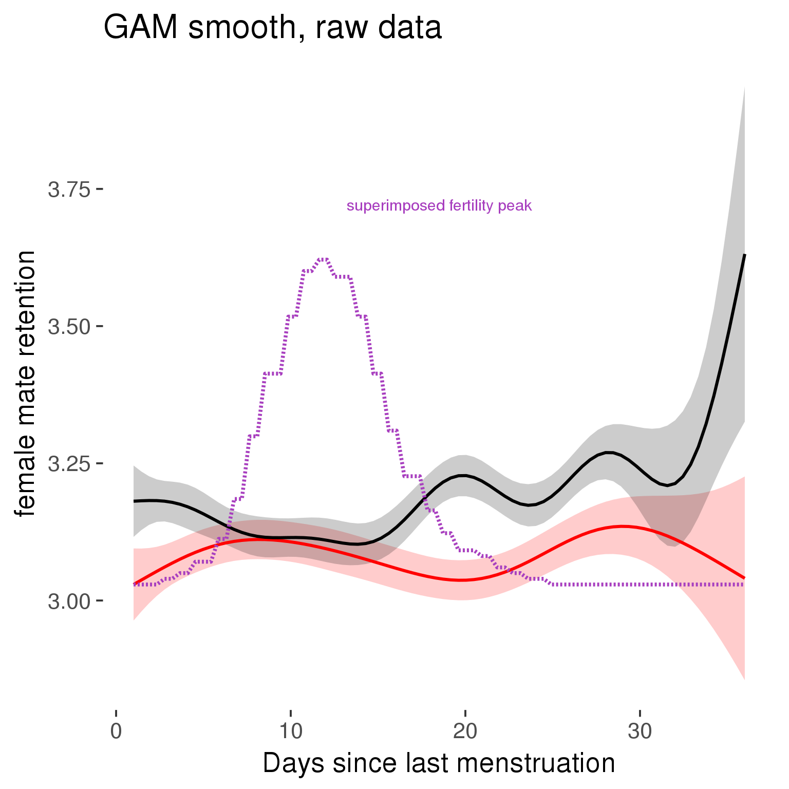
Means and standard errors over raw data
Nothing partialled out, just straight means with bootstrapped confidence intervals.
tryCatch({
trend_plot = ggplot(tmp,aes_string(x = "RCD", y = outcome, colour = "included")) +
geom_pointrange(size = 0.8, stat = 'summary', fun.data = "mean_cl_boot")
}, error = function(e){cat_message(e, "danger")})
tryCatch({
trend_data = ggplot_build(trend_plot)$data[[1]]
}, error = function(e){cat_message(e, "danger")})
trend_data$RCD = round(trend_data$x)
trend_data = left_join(trend_data, tmp %>% select(real, RCD,fertile) %>% unique(), by = "RCD")
trend_data %>%
filter(real == TRUE) %>%
mutate(superimposed = ( ( (fertile - 0.01)/0.58) * (max(y)-min(y) ) ) + min(y) ) ->
trend_data
plot3 = ggplot(trend_data) +
geom_pointrange(aes(x = x, y = y, ymin = ymin,ymax = ymax, colour = factor(group)), size = 0.8, stat = "identity", alpha = 0.6, position = position_dodge(width = .5)) +
scale_x_continuous("Days until next menstruation") +
geom_line(aes(x= x, y = superimposed), color = "#a83fbf", size = 1, linetype = 'dashed') +
annotate("text",x = mean(trend_data$x), y = max(trend_data$superimposed,na.rm=T) + 0.1, label = 'superimposed fertility peak', color = "#a83fbf") +
scale_y_continuous(outcome_label) +
ggtitle("Means with standard errors, raw data") +
scale_color_manual("Contraception status",values = c("2"="black","1"= "red"), labels = c("2"="hormonally\ncontracepting","1"="cycling"), guide = F) +
scale_fill_manual("Contraception status",values = c("2"="black","1"= "red"), labels = c("2"="hormonally\ncontracepting","1"="cycling"), guide = F)
suppressWarnings(print(plot3))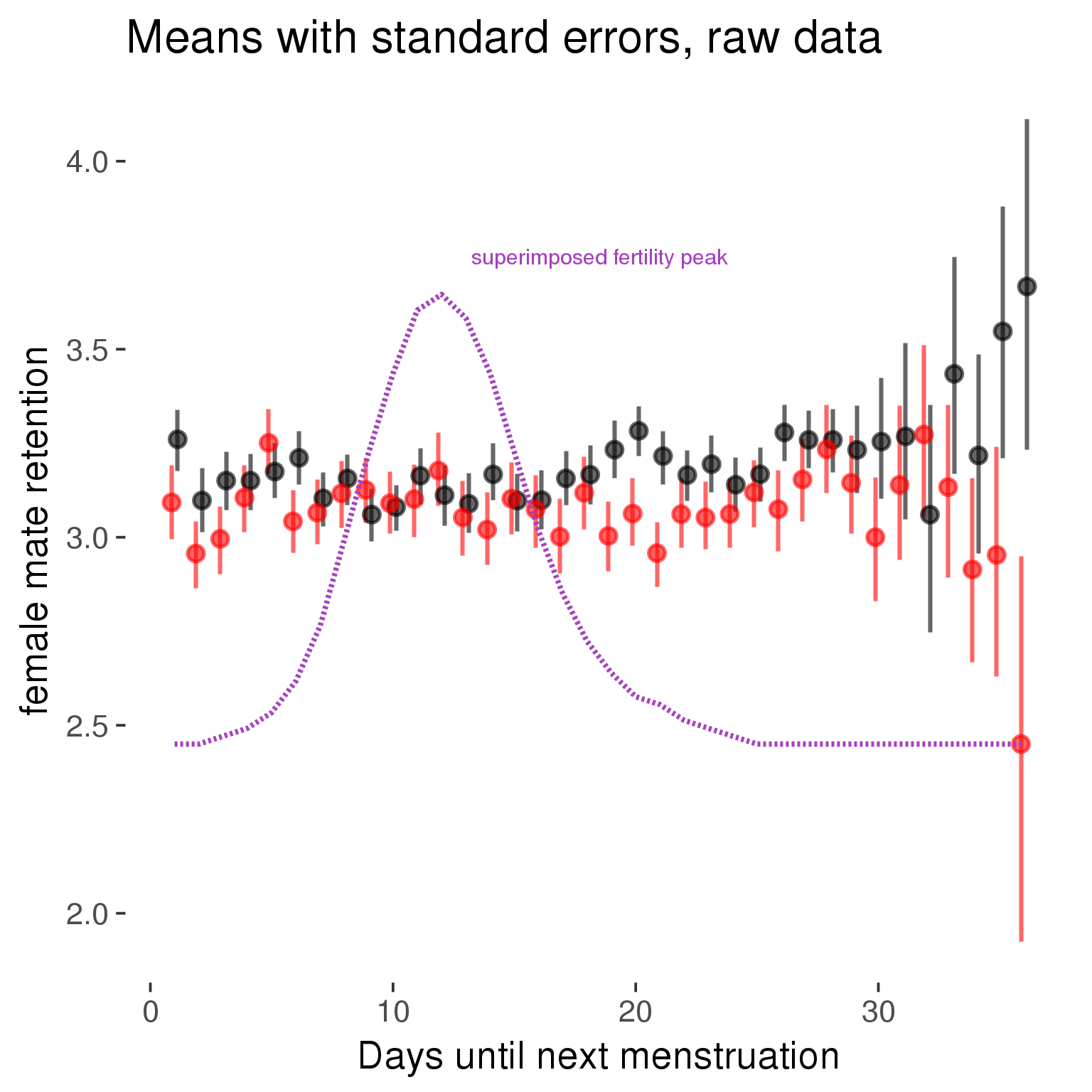
Cycle lengths from 27 to 30
Backward-counted
model %>%
plot_curve(diary %>% filter(minimum_cycle_length_diary <= 30, minimum_cycle_length_diary >= 27) %>% mutate(fertile=prc_stirn_b))outcome = names(model@frame)[1]
outcome_label = recode(str_replace_all(str_replace_all(str_replace_all(outcome, "_", " "), " pair", "-pair"), " 1", ""),
"desirability 1" = "self-perceived desirability",
"NARQ admiration" = "narcissistic admiration",
"NARQ rivalry" = "narcissistic rivalry",
"extra-pair" = "extra-pair desire & behaviour",
"had sexual intercourse" = "sexual intercourse")
library(ggplot2)
# form a subset and run the model without the hormonal contraception and the fertility predictors
tmp = diary %>%
filter(!is.na(fertile), !is.na(included),
RCD > -1 * minimum_cycle_length_diary, RCD > -40)
new_form = update.formula(formula(model), new = . ~ . - fertile * included)
tmp$residuals = residuals(update(model, new_form, data = tmp , na.action = na.exclude))
tmp = tmp %>%
filter(!is.na(RCD), !is.na(residuals))
rcd_min = min(tmp$RCD)
tmp$real = FALSE
tmp_before = tmp
tmp_before$RCD = tmp_before$RCD + min(tmp$RCD) - 1
tmp_after = tmp
tmp_after$RCD = tmp_after$RCD - min(tmp$RCD) + 1
tmp$real = TRUE
tmp = bind_rows(tmp_before %>% filter(RCD > rcd_min - 11), tmp, tmp_after %>% filter(RCD < 11))GAM smooth on residuals
Here, we partialled out menstruation and individual random effects, then superimposed estimated probability of being in the fertile window scaled to the range of the estimated means. To address the periodicity of the cycle, we prepended and appended ten days of the timeseries to the end and the beginning of the timeseries. We then estimated the GAM and cut off the appended subsets before plotting.
tryCatch({
trend_plot = ggplot(tmp,aes(x = RCD, y = residuals, colour = included)) +
stat_smooth(geom = 'smooth',size = 0.8, fill = "#9ECAE1", method = 'gam', formula = y ~ s(x))
}, error = function(e){cat_message(e, "danger")})
tryCatch({
trend_data = ggplot_build(trend_plot)$data[[1]]
}, error = function(e){cat_message(e, "danger")})
trend_data$RCD = round(trend_data$x)
trend_data = left_join(trend_data, tmp %>% select(real, RCD,fertile) %>% unique(), by = "RCD")
trend_data %>%
filter(real == TRUE) %>%
mutate(superimposed = ( ( (fertile - 0.01)/0.58) * (max(y)-min(y) ) ) + min(y) ) ->
trend_data
ggplot(trend_data) +
geom_ribbon(aes(x = x, ymin = ymin, ymax = ymax, fill = factor(group)), alpha = 0.2) +
geom_line(aes(x = x, y = y, colour = factor(group)), size = 0.8, stat = "identity") +
scale_x_continuous(caption_x) +
geom_line(aes(x = x, y = superimposed), color = "#a83fbf", size = 1, linetype = 'dashed') +
annotate("text",x = mean(trend_data$x), y = max(trend_data$superimposed,na.rm=T) + 0.1, label = 'superimposed fertility peak', color = "#a83fbf") +
scale_y_continuous(outcome_label) +
ggtitle("GAM smooth, residuals") +
scale_color_manual("Contraception status",values = c("2"="black","1"= "red"), labels = c("2"="hormonally\ncontracepting","1"="cycling"), guide = F) +
scale_fill_manual("Contraception status",values = c("2"="black","1"= "red"), labels = c("2"="hormonally\ncontracepting","1"="cycling"), guide = F)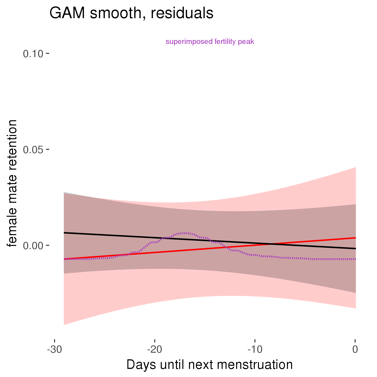
GAM smooth on raw data
As before, but without partialling anything out.
tryCatch({
trend_plot = ggplot(tmp,aes_string(x = "RCD", y = outcome, colour = "included")) +
stat_smooth(geom = 'smooth',size = 0.8, fill = "#9ECAE1", method = 'gam', formula = y ~ s(x))
}, error = function(e){cat_message(e, "danger")})
tryCatch({
trend_data = ggplot_build(trend_plot)$data[[1]]
}, error = function(e){cat_message(e, "danger")})
trend_data$RCD = round(trend_data$x)
trend_data = left_join(trend_data, tmp %>% select(real, RCD,fertile) %>% unique(), by = "RCD")
trend_data %>%
filter(real == TRUE) %>%
mutate(superimposed = ( ( (fertile - 0.01)/0.58) * (max(y)-min(y) ) ) + min(y) ) ->
trend_data
plot1b = ggplot(trend_data) +
geom_ribbon(aes(x = x, ymin = ymin, ymax = ymax, fill = factor(group)), alpha = 0.2) +
geom_line(aes(x = x, y = y, colour = factor(group)), size = 0.8, stat = "identity") +
scale_x_continuous(caption_x) +
geom_line(aes(x = x, y = superimposed), color = "#a83fbf", size = 1, linetype = 'dashed') +
annotate("text",x = mean(trend_data$x), y = max(trend_data$superimposed,na.rm=T) + 0.1, label = 'superimposed fertility peak', color = "#a83fbf") +
scale_y_continuous(outcome_label) +
ggtitle("GAM smooth, raw data") +
scale_color_manual("Contraception status",values = c("2"="black","1"= "red"), labels = c("2"="hormonally\ncontracepting","1"="cycling"), guide = F) +
scale_fill_manual("Contraception status",values = c("2"="black","1"= "red"), labels = c("2"="hormonally\ncontracepting","1"="cycling"), guide = F)
suppressWarnings(print(plot1b))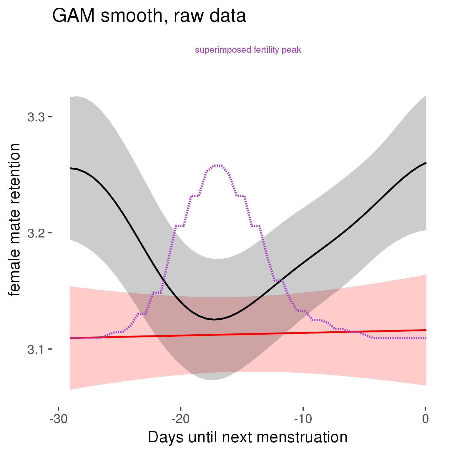
Means and standard errors over raw data
Nothing partialled out, just straight means with bootstrapped confidence intervals.
tryCatch({
trend_plot = ggplot(tmp,aes_string(x = "RCD", y = outcome, colour = "included")) +
geom_pointrange(size = 0.8, stat = 'summary', fun.data = "mean_cl_boot")
}, error = function(e){cat_message(e, "danger")})
tryCatch({
trend_data = ggplot_build(trend_plot)$data[[1]]
}, error = function(e){cat_message(e, "danger")})
trend_data$RCD = round(trend_data$x)
trend_data = left_join(trend_data, tmp %>% select(real, RCD,fertile) %>% unique(), by = "RCD")
trend_data %>%
filter(real == TRUE) %>%
mutate(superimposed = ( ( (fertile - 0.01)/0.58) * (max(y)-min(y) ) ) + min(y) ) ->
trend_data
plot3 = ggplot(trend_data) +
geom_pointrange(aes(x = x, y = y, ymin = ymin,ymax = ymax, colour = factor(group)), size = 0.8, stat = "identity", alpha = 0.6, position = position_dodge(width = .5)) +
scale_x_continuous("Days until next menstruation") +
geom_line(aes(x= x, y = superimposed), color = "#a83fbf", size = 1, linetype = 'dashed') +
annotate("text",x = mean(trend_data$x), y = max(trend_data$superimposed,na.rm=T) + 0.1, label = 'superimposed fertility peak', color = "#a83fbf") +
scale_y_continuous(outcome_label) +
ggtitle("Means with standard errors, raw data") +
scale_color_manual("Contraception status",values = c("2"="black","1"= "red"), labels = c("2"="hormonally\ncontracepting","1"="cycling"), guide = F) +
scale_fill_manual("Contraception status",values = c("2"="black","1"= "red"), labels = c("2"="hormonally\ncontracepting","1"="cycling"), guide = F)
suppressWarnings(print(plot3))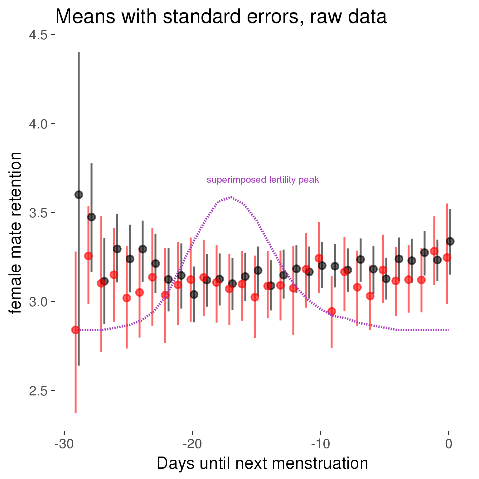
Forward-counted
model %>%
plot_curve(diary %>% filter(minimum_cycle_length_diary <= 30, minimum_cycle_length_diary >= 27) %>% mutate(RCD = FCD, fertile = prc_stirn_b_forward_counted), caption_x = "Days since last menstruation")outcome = names(model@frame)[1]
outcome_label = recode(str_replace_all(str_replace_all(str_replace_all(outcome, "_", " "), " pair", "-pair"), " 1", ""),
"desirability 1" = "self-perceived desirability",
"NARQ admiration" = "narcissistic admiration",
"NARQ rivalry" = "narcissistic rivalry",
"extra-pair" = "extra-pair desire & behaviour",
"had sexual intercourse" = "sexual intercourse")
library(ggplot2)
# form a subset and run the model without the hormonal contraception and the fertility predictors
tmp = diary %>%
filter(!is.na(fertile), !is.na(included),
RCD > -1 * minimum_cycle_length_diary, RCD > -40)
new_form = update.formula(formula(model), new = . ~ . - fertile * included)
tmp$residuals = residuals(update(model, new_form, data = tmp , na.action = na.exclude))
tmp = tmp %>%
filter(!is.na(RCD), !is.na(residuals))
rcd_min = min(tmp$RCD)
tmp$real = FALSE
tmp_before = tmp
tmp_before$RCD = tmp_before$RCD + min(tmp$RCD) - 1
tmp_after = tmp
tmp_after$RCD = tmp_after$RCD - min(tmp$RCD) + 1
tmp$real = TRUE
tmp = bind_rows(tmp_before %>% filter(RCD > rcd_min - 11), tmp, tmp_after %>% filter(RCD < 11))GAM smooth on residuals
Here, we partialled out menstruation and individual random effects, then superimposed estimated probability of being in the fertile window scaled to the range of the estimated means. To address the periodicity of the cycle, we prepended and appended ten days of the timeseries to the end and the beginning of the timeseries. We then estimated the GAM and cut off the appended subsets before plotting.
tryCatch({
trend_plot = ggplot(tmp,aes(x = RCD, y = residuals, colour = included)) +
stat_smooth(geom = 'smooth',size = 0.8, fill = "#9ECAE1", method = 'gam', formula = y ~ s(x))
}, error = function(e){cat_message(e, "danger")})
tryCatch({
trend_data = ggplot_build(trend_plot)$data[[1]]
}, error = function(e){cat_message(e, "danger")})
trend_data$RCD = round(trend_data$x)
trend_data = left_join(trend_data, tmp %>% select(real, RCD,fertile) %>% unique(), by = "RCD")
trend_data %>%
filter(real == TRUE) %>%
mutate(superimposed = ( ( (fertile - 0.01)/0.58) * (max(y)-min(y) ) ) + min(y) ) ->
trend_data
ggplot(trend_data) +
geom_ribbon(aes(x = x, ymin = ymin, ymax = ymax, fill = factor(group)), alpha = 0.2) +
geom_line(aes(x = x, y = y, colour = factor(group)), size = 0.8, stat = "identity") +
scale_x_continuous(caption_x) +
geom_line(aes(x = x, y = superimposed), color = "#a83fbf", size = 1, linetype = 'dashed') +
annotate("text",x = mean(trend_data$x), y = max(trend_data$superimposed,na.rm=T) + 0.1, label = 'superimposed fertility peak', color = "#a83fbf") +
scale_y_continuous(outcome_label) +
ggtitle("GAM smooth, residuals") +
scale_color_manual("Contraception status",values = c("2"="black","1"= "red"), labels = c("2"="hormonally\ncontracepting","1"="cycling"), guide = F) +
scale_fill_manual("Contraception status",values = c("2"="black","1"= "red"), labels = c("2"="hormonally\ncontracepting","1"="cycling"), guide = F)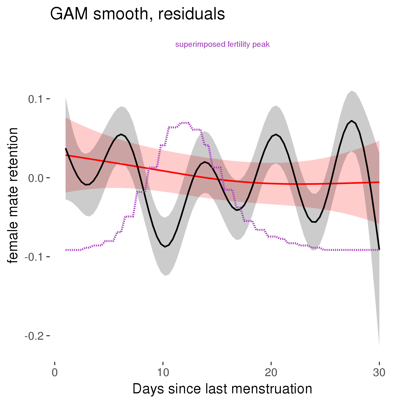
GAM smooth on raw data
As before, but without partialling anything out.
tryCatch({
trend_plot = ggplot(tmp,aes_string(x = "RCD", y = outcome, colour = "included")) +
stat_smooth(geom = 'smooth',size = 0.8, fill = "#9ECAE1", method = 'gam', formula = y ~ s(x))
}, error = function(e){cat_message(e, "danger")})
tryCatch({
trend_data = ggplot_build(trend_plot)$data[[1]]
}, error = function(e){cat_message(e, "danger")})
trend_data$RCD = round(trend_data$x)
trend_data = left_join(trend_data, tmp %>% select(real, RCD,fertile) %>% unique(), by = "RCD")
trend_data %>%
filter(real == TRUE) %>%
mutate(superimposed = ( ( (fertile - 0.01)/0.58) * (max(y)-min(y) ) ) + min(y) ) ->
trend_data
plot1b = ggplot(trend_data) +
geom_ribbon(aes(x = x, ymin = ymin, ymax = ymax, fill = factor(group)), alpha = 0.2) +
geom_line(aes(x = x, y = y, colour = factor(group)), size = 0.8, stat = "identity") +
scale_x_continuous(caption_x) +
geom_line(aes(x = x, y = superimposed), color = "#a83fbf", size = 1, linetype = 'dashed') +
annotate("text",x = mean(trend_data$x), y = max(trend_data$superimposed,na.rm=T) + 0.1, label = 'superimposed fertility peak', color = "#a83fbf") +
scale_y_continuous(outcome_label) +
ggtitle("GAM smooth, raw data") +
scale_color_manual("Contraception status",values = c("2"="black","1"= "red"), labels = c("2"="hormonally\ncontracepting","1"="cycling"), guide = F) +
scale_fill_manual("Contraception status",values = c("2"="black","1"= "red"), labels = c("2"="hormonally\ncontracepting","1"="cycling"), guide = F)
suppressWarnings(print(plot1b))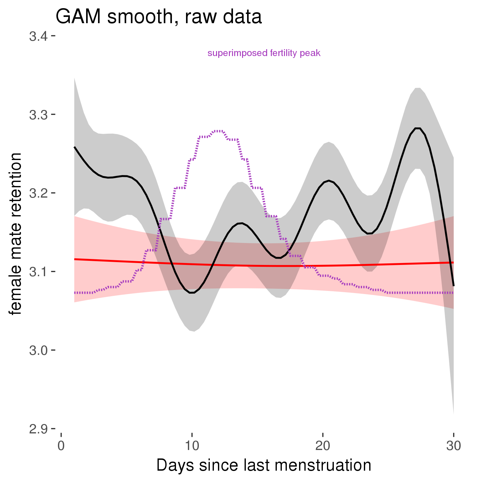
Means and standard errors over raw data
Nothing partialled out, just straight means with bootstrapped confidence intervals.
tryCatch({
trend_plot = ggplot(tmp,aes_string(x = "RCD", y = outcome, colour = "included")) +
geom_pointrange(size = 0.8, stat = 'summary', fun.data = "mean_cl_boot")
}, error = function(e){cat_message(e, "danger")})
tryCatch({
trend_data = ggplot_build(trend_plot)$data[[1]]
}, error = function(e){cat_message(e, "danger")})
trend_data$RCD = round(trend_data$x)
trend_data = left_join(trend_data, tmp %>% select(real, RCD,fertile) %>% unique(), by = "RCD")
trend_data %>%
filter(real == TRUE) %>%
mutate(superimposed = ( ( (fertile - 0.01)/0.58) * (max(y)-min(y) ) ) + min(y) ) ->
trend_data
plot3 = ggplot(trend_data) +
geom_pointrange(aes(x = x, y = y, ymin = ymin,ymax = ymax, colour = factor(group)), size = 0.8, stat = "identity", alpha = 0.6, position = position_dodge(width = .5)) +
scale_x_continuous("Days until next menstruation") +
geom_line(aes(x= x, y = superimposed), color = "#a83fbf", size = 1, linetype = 'dashed') +
annotate("text",x = mean(trend_data$x), y = max(trend_data$superimposed,na.rm=T) + 0.1, label = 'superimposed fertility peak', color = "#a83fbf") +
scale_y_continuous(outcome_label) +
ggtitle("Means with standard errors, raw data") +
scale_color_manual("Contraception status",values = c("2"="black","1"= "red"), labels = c("2"="hormonally\ncontracepting","1"="cycling"), guide = F) +
scale_fill_manual("Contraception status",values = c("2"="black","1"= "red"), labels = c("2"="hormonally\ncontracepting","1"="cycling"), guide = F)
suppressWarnings(print(plot3))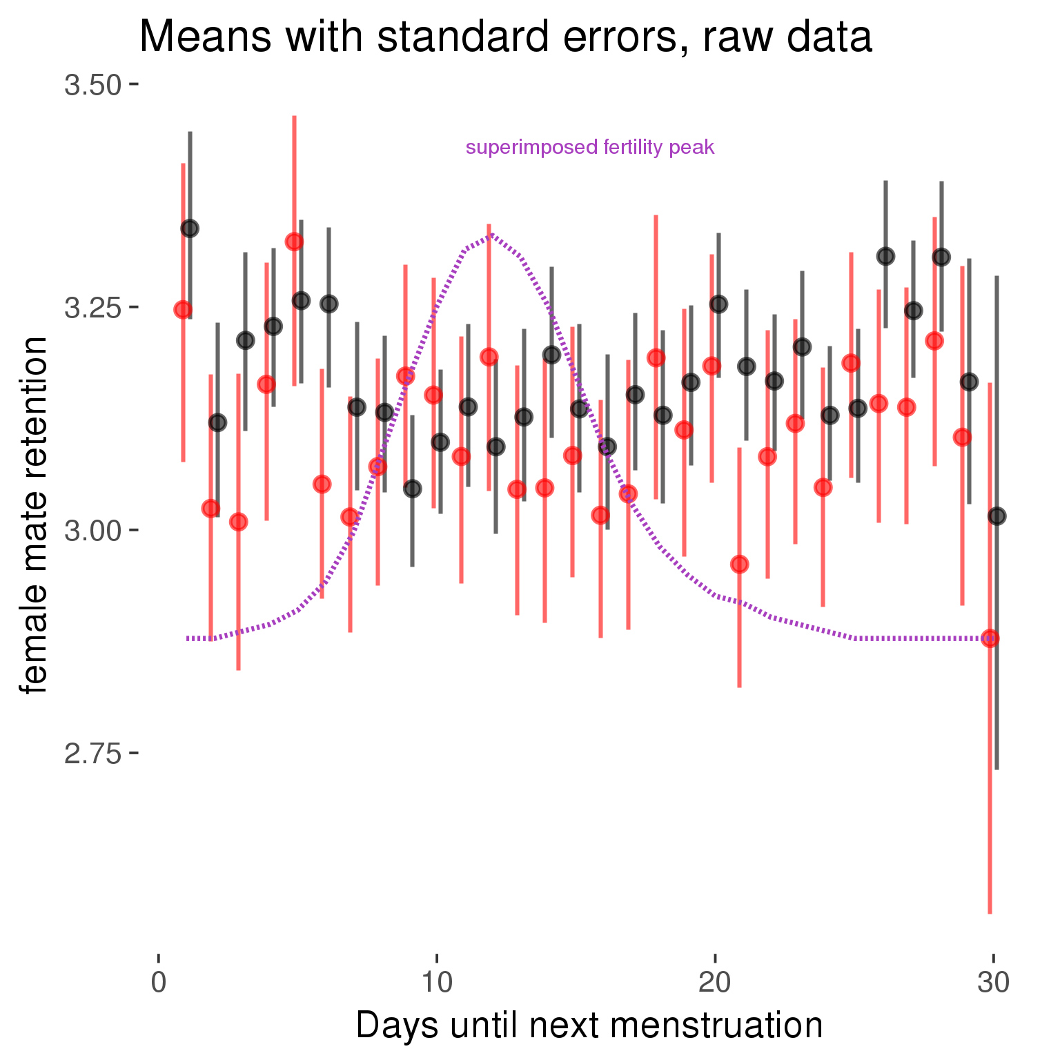
Robustness checks
M_r1: Random slopes for conception risk and menstruation
tryCatch({
# refit model with random effects for fertile and menstruation dummies
with_ind_diff = update(model, formula = . ~ . - (1| person) + (1 + fertile + menstruation | person))
# pull the random effects, format as tibble
rand = coef(with_ind_diff)$person %>%
tibble::rownames_to_column("person") %>%
mutate(person = as.numeric(person))
# pull the fixed effects
fixd = data.frame(fixef(with_ind_diff)) %>%
tibble::rownames_to_column("effect")
names(fixd) = c("effect", "pop_effect_size")
# pull apart the coefficients so that we can account for the fact that the random effect variation implicitly includes HC explaining the mean population-level effect of fertile/menstruation dummies among HC users
fixd = fixd %>%
separate(effect, c("included", "effect"), sep = ":", fill = "left") %>%
mutate(included = if_else(is.na(included), "cycling", str_replace(included, "included", "")))
fixd[2,c("included", "effect")] = c("horm_contra", "(Intercept)")
rand = rand %>%
# merge diary data on the random effects, so that we know who is a HC users and who isn't
inner_join(diary %>% select(person, included) %>% unique(), by = 'person') %>%
# gather into long format, to have the dataset by predictor
gather(effect, value, -person, -included) %>%
inner_join(fixd, by = c('effect', 'included')) %>%
# pull the fixed effects
mutate(
# only for those who are HC users, add the moderated population effect size for this effect (the random effects have the reference category mean)
value = if_else(included == "horm_contra", value + pop_effect_size, value),
effect = recode(effect, "includedhorm_contra" = "HC user",
"includedhorm_contra:fertile" = "HC user x fertile",
"includedhorm_contra:menstruationpre" = "HC user x premens.",
"includedhorm_contra:menstruationyes" = "HC user x mens.",
"menstruationyes" = "mens.",
"menstruationpre" = "premens.")) %>%
group_by(included, effect) %>%
# filter out predictors that aren't modelled as varying/random
filter(sd(value) > 0)
# plot dot plot of random effects
print(
ggplot(rand, aes(x = included, y = value, color = included, fill = included)) +
facet_wrap( ~ effect, scales = "free") +
# geom_violin(alpha = 0.4, size = 0) +
geom_dotplot(binaxis='y', dotsize = 0.1, method = "histodot") +
# geom_jitter(alpha = 0.05) +
coord_flip() +
geom_pointrange(stat = 'summary', fun.data = 'mean_sdl', color = 'darkred', size = 1.2) +
scale_color_manual("Contraception status", values = c("horm_contra"="black","cycling"= "red"), labels = c("horm_contra"="hormonally\ncontracepting","cycling"="cycling"), guide = F) +
scale_fill_manual("Contraception status", values = c("horm_contra"="black","cycling"= "red"), labels = c("horm_contra"="hormonally\ncontracepting","1"="cycling"), guide = F) +
ggtitle("M_r1: allowing participant-varying slopes", subtitle = "for the conception risk measure and the menstruation dummies") +
scale_x_discrete("Hormonal contraception", breaks = c("horm_contra", "cycling"), labels = c("yes", "no")) +
scale_y_continuous("Random effect size distribution"))
print_summary(with_ind_diff)
cat(pander(anova(model, with_ind_diff)))
}, error = function(e){
with_ind_diff = model
cat_message(e, "danger")
})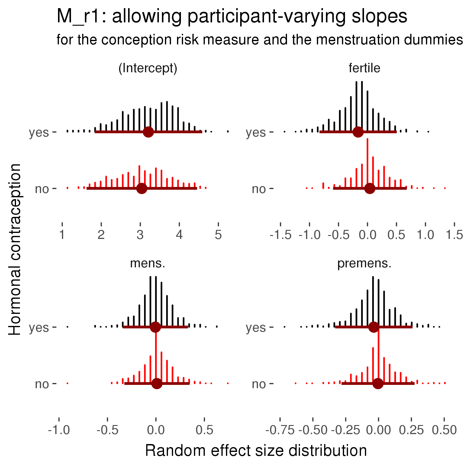
Linear mixed model fit by REML ['lmerMod']
Formula: female_mate_retention ~ included + menstruation + fertile + fertile_mean +
(1 + fertile + menstruation | person) + included:menstruation + included:fertile
Data: diary
REML criterion at convergence: 69356
Scaled residuals:
Min 1Q Median 3Q Max
-4.046 -0.615 -0.005 0.615 4.665
Random effects:
Groups Name Variance Std.Dev. Corr
person (Intercept) 0.5611 0.749
fertile 0.4076 0.638 -0.17
menstruationpre 0.0886 0.298 -0.10 0.26
menstruationyes 0.1057 0.325 -0.12 0.32 0.43
Residual 0.6777 0.823
Number of obs: 26681, groups: person, 1054
Fixed effects:
Estimate Std. Error t value
(Intercept) 3.03783 0.06408 47.4
includedhorm_contra 0.16921 0.05287 3.2
menstruationpre -0.00405 0.03074 -0.1
menstruationyes 0.01003 0.03025 0.3
fertile 0.04044 0.06290 0.6
fertile_mean -0.12877 0.29312 -0.4
includedhorm_contra:menstruationpre -0.03192 0.03946 -0.8
includedhorm_contra:menstruationyes -0.01562 0.03940 -0.4
includedhorm_contra:fertile -0.20147 0.07987 -2.5
Correlation of Fixed Effects:
(Intr) incld_ mnstrtnp mnstrtny fertil frtl_m inclddhrm_cntr:mnstrtnp
inclddhrm_c -0.477
menstrutnpr -0.161 0.201
menstrutnys -0.165 0.205 0.400
fertile -0.168 0.273 0.397 0.361
fertile_men -0.768 -0.026 -0.006 -0.004 -0.072
inclddhrm_cntr:mnstrtnp 0.133 -0.252 -0.779 -0.312 -0.309 -0.005
inclddhrm_cntr:mnstrtny 0.132 -0.254 -0.307 -0.768 -0.277 -0.004 0.390
inclddhrm_cntr:f 0.168 -0.346 -0.312 -0.284 -0.784 0.012 0.397
inclddhrm_cntr:mnstrtny
inclddhrm_c
menstrutnpr
menstrutnys
fertile
fertile_men
inclddhrm_cntr:mnstrtnp
inclddhrm_cntr:mnstrtny
inclddhrm_cntr:f 0.358
refitting model(s) with ML (instead of REML)
| Df | AIC | BIC | logLik | deviance | Chisq | Chi Df | Pr(>Chisq) | |
|---|---|---|---|---|---|---|---|---|
| object | 11 | 69586 | 69676 | -34782 | 69564 | NA | NA | NA |
| ..1 | 20 | 69356 | 69520 | -34658 | 69316 | 247.5 | 9 | 3.347e-48 |
robustness_check_ovu_shift(model, diary)M_e: Exclusion criteria
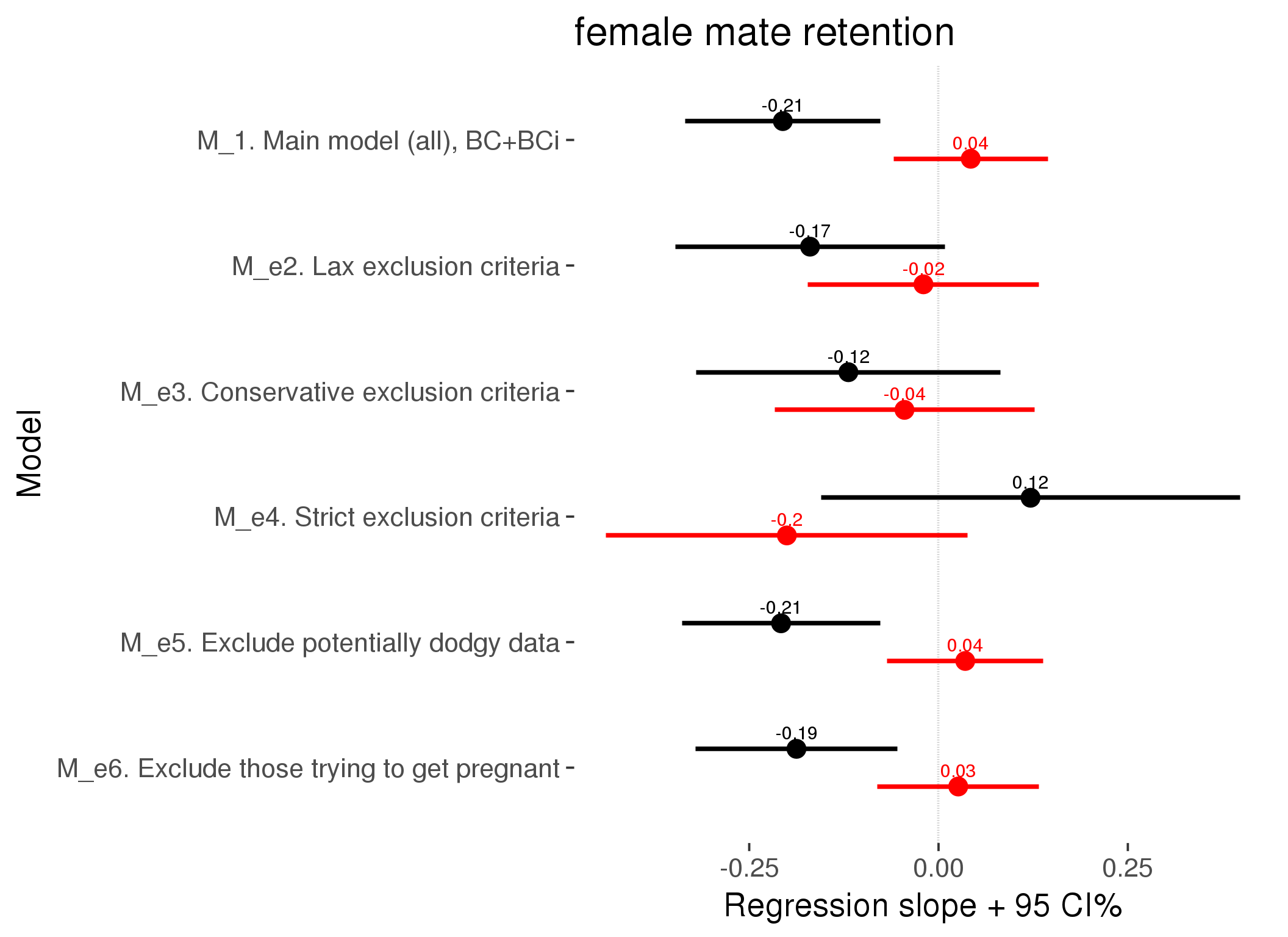
M_p: Predictors
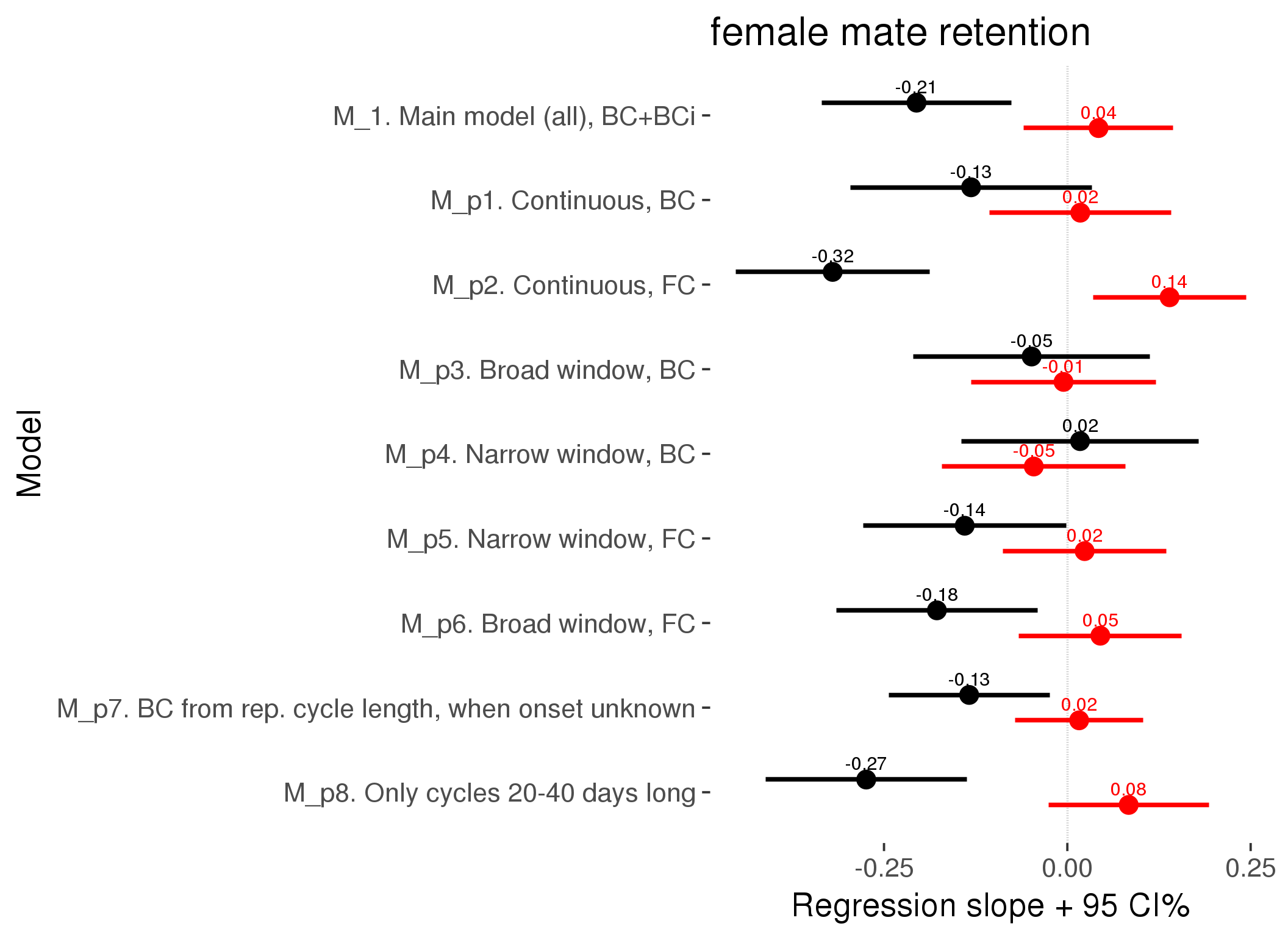
M_c: Covariates, controls, autocorrelation
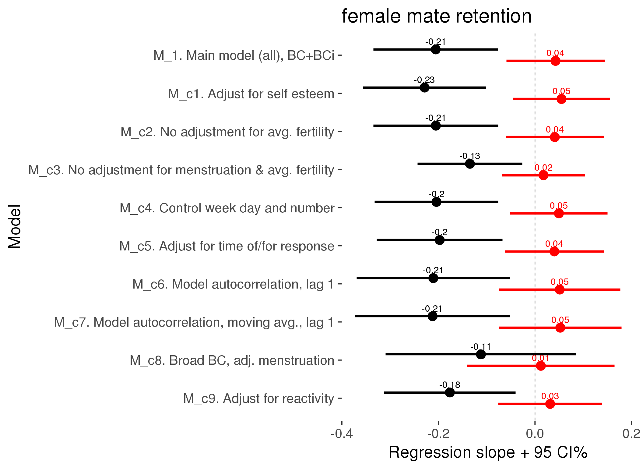
Linear mixed model fit by REML ['lmerMod']
REML criterion at convergence: 63259
Scaled residuals:
Min 1Q Median 3Q Max
-4.328 -0.626 -0.003 0.628 4.479
Random effects:
Groups Name Variance Std.Dev.
person (Intercept) 0.5486 0.741
Xr.2 s(days_filled_out):includedhorm_contra 0.2220 0.471
Xr.1 s(days_filled_out):includedcycling 0.0851 0.292
Xr.0 s(day_number):includedhorm_contra 0.3100 0.557
Xr s(day_number):includedcycling 0.0603 0.246
Residual 0.6948 0.834
Number of obs: 24378, groups: person, 1054; Xr.2, 8; Xr.1, 8; Xr.0, 8; Xr, 8
Fixed effects:
Estimate Std. Error t value
X(Intercept) 3.00767 0.06406 46.9
Xincludedhorm_contra 0.17730 0.05295 3.3
Xmenstruationpre 0.00762 0.02663 0.3
Xmenstruationyes 0.01859 0.02558 0.7
Xfertile 0.03141 0.05485 0.6
Xfertile_mean -0.10781 0.29148 -0.4
Xincludedhorm_contra:menstruationpre -0.03697 0.03417 -1.1
Xincludedhorm_contra:menstruationyes -0.02298 0.03348 -0.7
Xincludedhorm_contra:fertile -0.17630 0.06947 -2.5
Xs(day_number):includedcyclingFx1 0.26561 0.09355 2.8
Xs(day_number):includedhorm_contraFx1 0.53463 0.13858 3.9
Xs(days_filled_out):includedcyclingFx1 -0.16648 0.10136 -1.6
Xs(days_filled_out):includedhorm_contraFx1 -0.49292 0.13237 -3.7
Family: gaussian
Link function: identity
Formula:
female_mate_retention ~ included + menstruation + fertile + fertile_mean +
s(day_number, by = included) + s(days_filled_out, by = included) +
included:menstruation + included:fertile
Parametric coefficients:
Estimate Std. Error t value Pr(>|t|)
(Intercept) 3.00767 0.06406 46.95 < 2e-16 ***
includedhorm_contra 0.17730 0.05295 3.35 0.00081 ***
menstruationpre 0.00762 0.02663 0.29 0.77470
menstruationyes 0.01859 0.02558 0.73 0.46734
fertile 0.03141 0.05485 0.57 0.56688
fertile_mean -0.10781 0.29148 -0.37 0.71147
includedhorm_contra:menstruationpre -0.03697 0.03417 -1.08 0.27932
includedhorm_contra:menstruationyes -0.02298 0.03348 -0.69 0.49241
includedhorm_contra:fertile -0.17630 0.06947 -2.54 0.01116 *
---
Signif. codes: 0 '***' 0.001 '**' 0.01 '*' 0.05 '.' 0.1 ' ' 1
Approximate significance of smooth terms:
edf Ref.df F p-value
s(day_number):includedcycling 3.41 3.41 6.04 0.00023 ***
s(day_number):includedhorm_contra 5.70 5.70 8.36 0.000000013 ***
s(days_filled_out):includedcycling 3.86 3.86 5.63 0.00029 ***
s(days_filled_out):includedhorm_contra 5.18 5.18 7.95 0.000000127 ***
---
Signif. codes: 0 '***' 0.001 '**' 0.01 '*' 0.05 '.' 0.1 ' ' 1
R-sq.(adj) = 0.00129
lmer.REML = 63259 Scale est. = 0.69478 n = 24378
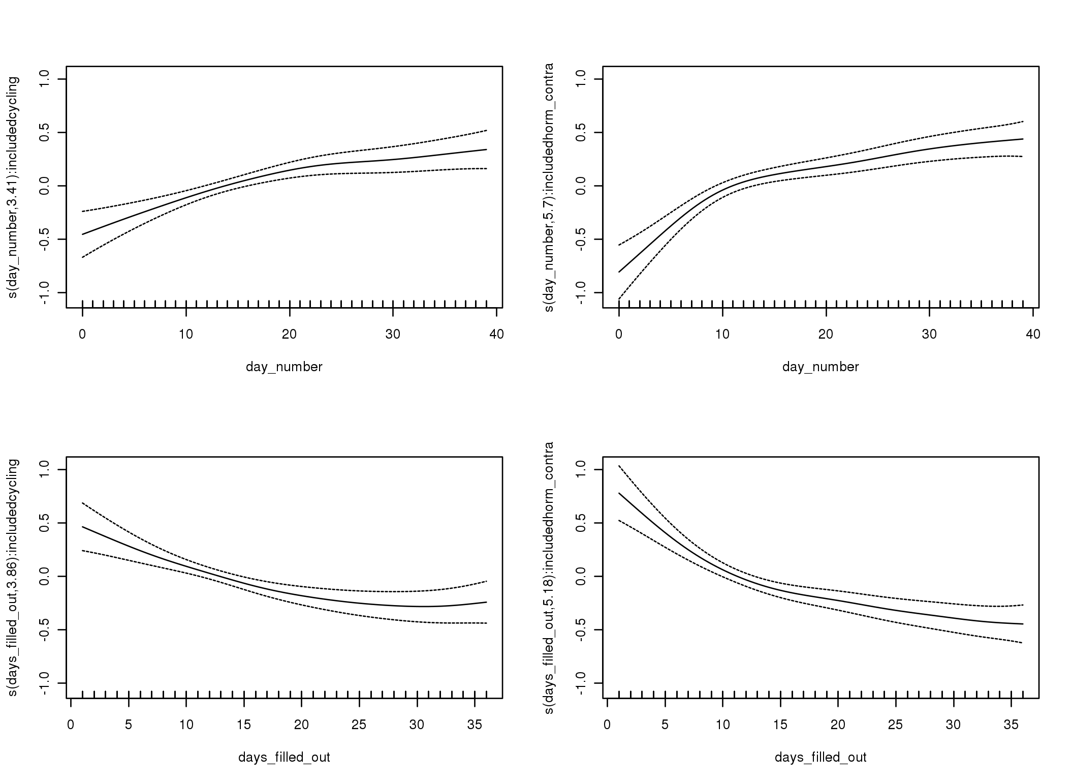
Linear mixed-effects model fit by REML
Data: diary
AIC BIC logLik
67786 67885 -33881
Random effects:
Formula: ~1 | person
(Intercept) Residual
StdDev: 0.7189 0.8567
Correlation Structure: ARMA(1,0)
Formula: ~day_number | person
Parameter estimate(s):
Phi1
0.3116
Fixed effects: female_mate_retention ~ included * (menstruation + fertile) + fertile_mean
Value Std.Error DF t-value p-value
(Intercept) 3.0457 0.06442 25621 47.28 0.0000
includedhorm_contra 0.1669 0.05307 1051 3.14 0.0017
menstruationpre -0.0064 0.03001 25621 -0.21 0.8319
menstruationyes 0.0089 0.02801 25621 0.32 0.7516
fertile 0.0511 0.06412 25621 0.80 0.4251
fertile_mean -0.1014 0.29528 1051 -0.34 0.7312
includedhorm_contra:menstruationpre -0.0325 0.03855 25621 -0.84 0.3995
includedhorm_contra:menstruationyes -0.0053 0.03649 25621 -0.14 0.8848
includedhorm_contra:fertile -0.2106 0.08112 25621 -2.60 0.0094
Correlation:
(Intr) incld_ mnstrtnp mnstrtny fertil frtl_m inclddhrm_cntr:mnstrtnp
includedhorm_contra -0.477
menstruationpre -0.177 0.222
menstruationyes -0.174 0.216 0.403
fertile -0.170 0.283 0.424 0.359
fertile_mean -0.768 -0.026 -0.008 -0.006 -0.080
includedhorm_contra:menstruationpre 0.145 -0.277 -0.778 -0.314 -0.329 -0.004
includedhorm_contra:menstruationyes 0.139 -0.264 -0.309 -0.767 -0.275 -0.003 0.388
includedhorm_contra:fertile 0.173 -0.358 -0.334 -0.283 -0.786 0.014 0.423
inclddhrm_cntr:mnstrtny
includedhorm_contra
menstruationpre
menstruationyes
fertile
fertile_mean
includedhorm_contra:menstruationpre
includedhorm_contra:menstruationyes
includedhorm_contra:fertile 0.352
Standardized Within-Group Residuals:
Min Q1 Med Q3 Max
-4.020627 -0.640672 -0.008752 0.613116 4.495209
Number of Observations: 26681
Number of Groups: 1054
Linear mixed-effects model fit by REML
Data: diary
AIC BIC logLik
67780 67887 -33877
Random effects:
Formula: ~1 | person
(Intercept) Residual
StdDev: 0.7174 0.8576
Correlation Structure: ARMA(1,1)
Formula: ~day_number | person
Parameter estimate(s):
Phi1 Theta1
0.37444 -0.06926
Fixed effects: female_mate_retention ~ included * (menstruation + fertile) + fertile_mean
Value Std.Error DF t-value p-value
(Intercept) 3.0453 0.06446 25621 47.25 0.0000
includedhorm_contra 0.1669 0.05312 1051 3.14 0.0017
menstruationpre -0.0060 0.03016 25621 -0.20 0.8410
menstruationyes 0.0077 0.02817 25621 0.27 0.7850
fertile 0.0524 0.06476 25621 0.81 0.4181
fertile_mean -0.1000 0.29550 1051 -0.34 0.7352
includedhorm_contra:menstruationpre -0.0326 0.03874 25621 -0.84 0.3994
includedhorm_contra:menstruationyes -0.0041 0.03668 25621 -0.11 0.9108
includedhorm_contra:fertile -0.2121 0.08192 25621 -2.59 0.0096
Correlation:
(Intr) incld_ mnstrtnp mnstrtny fertil frtl_m inclddhrm_cntr:mnstrtnp
includedhorm_contra -0.477
menstruationpre -0.177 0.222
menstruationyes -0.175 0.217 0.405
fertile -0.171 0.285 0.418 0.357
fertile_mean -0.768 -0.026 -0.007 -0.006 -0.081
includedhorm_contra:menstruationpre 0.146 -0.278 -0.778 -0.315 -0.325 -0.004
includedhorm_contra:menstruationyes 0.140 -0.266 -0.311 -0.768 -0.273 -0.003 0.390
includedhorm_contra:fertile 0.173 -0.359 -0.330 -0.282 -0.786 0.014 0.417
inclddhrm_cntr:mnstrtny
includedhorm_contra
menstruationpre
menstruationyes
fertile
fertile_mean
includedhorm_contra:menstruationpre
includedhorm_contra:menstruationyes
includedhorm_contra:fertile 0.350
Standardized Within-Group Residuals:
Min Q1 Med Q3 Max
-4.00397 -0.64073 -0.00894 0.61459 4.48421
Number of Observations: 26681
Number of Groups: 1054
M_d: Other designs
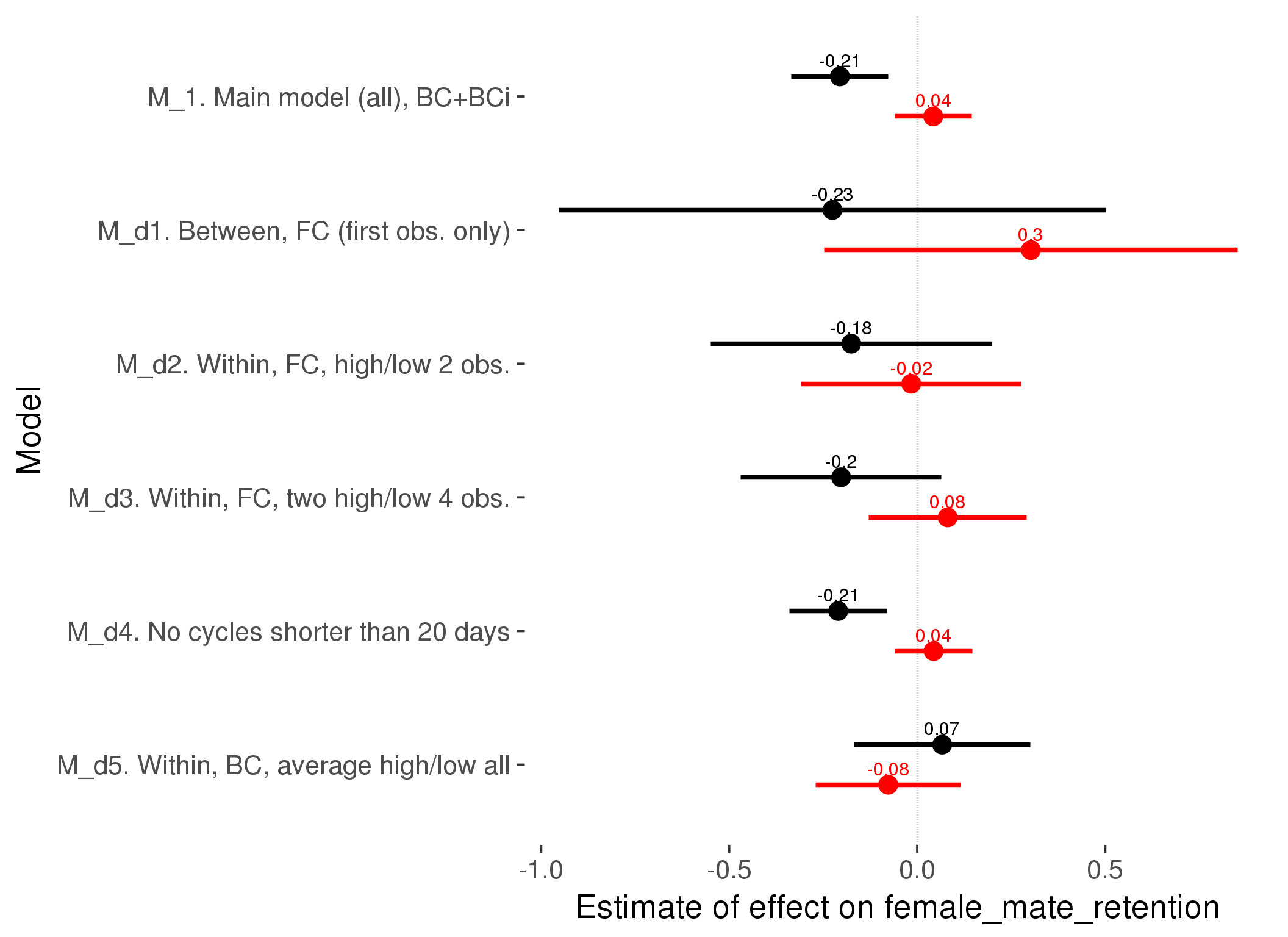
M_m1: Moderation by contraceptive method
Based on the sample with lax exclusion criteria. Users who used any hormonal contraception are classified as hormonal, users who use any awareness-based methods (counting, temperature-based) are classified as ‘fertility-awareness’, women who don’t fall into the before groups and use condoms, pessars, coitus interruptus etc. are classified as ‘barrie or abstinence’. Women who don’t use contraception or use other methods such as sterilisation are excluded from this analysis.
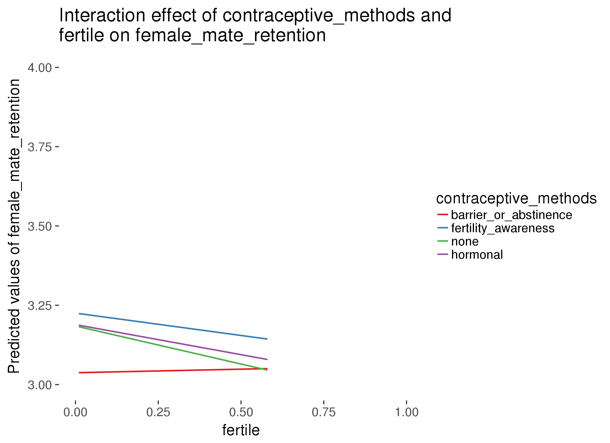
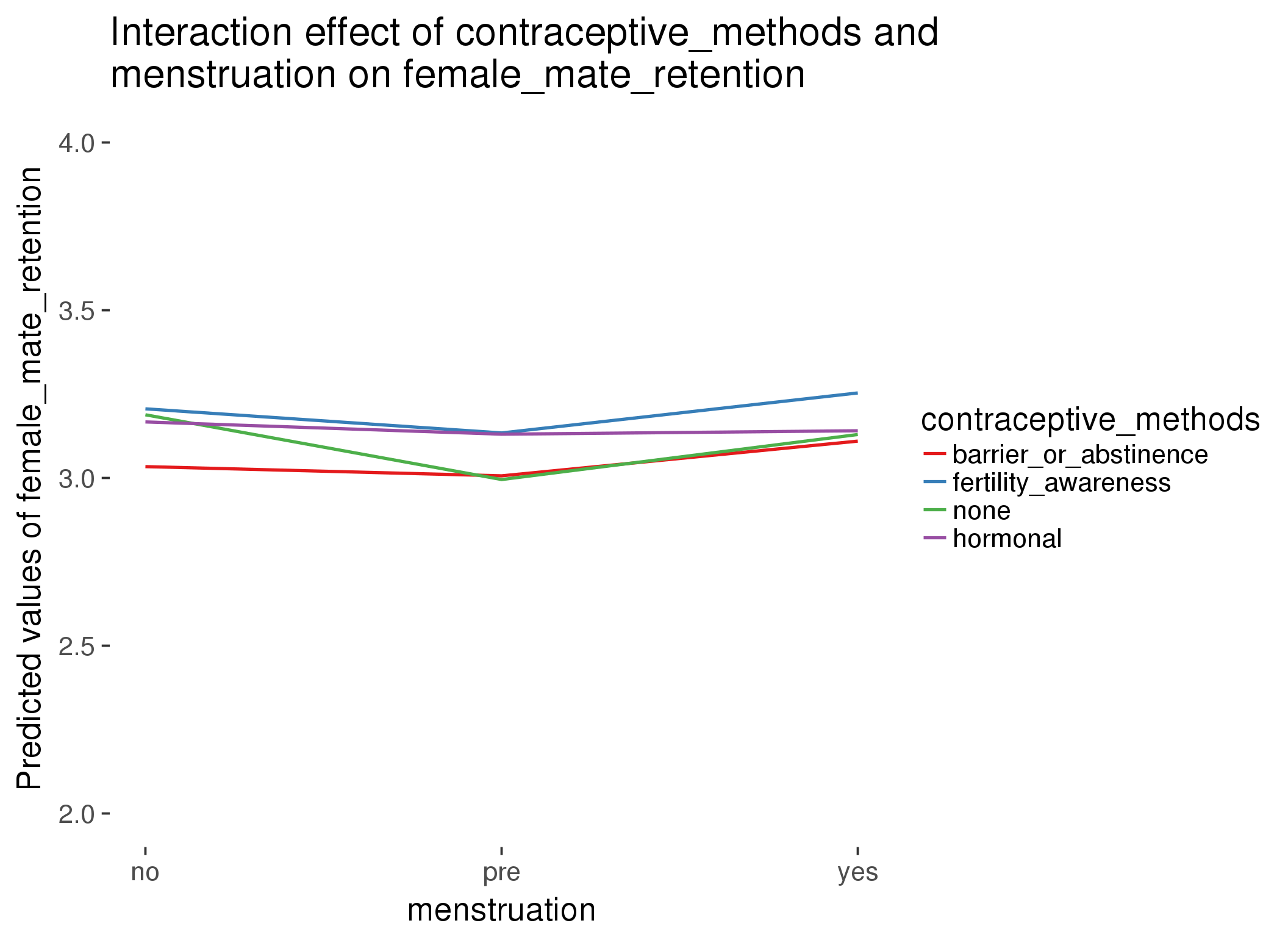
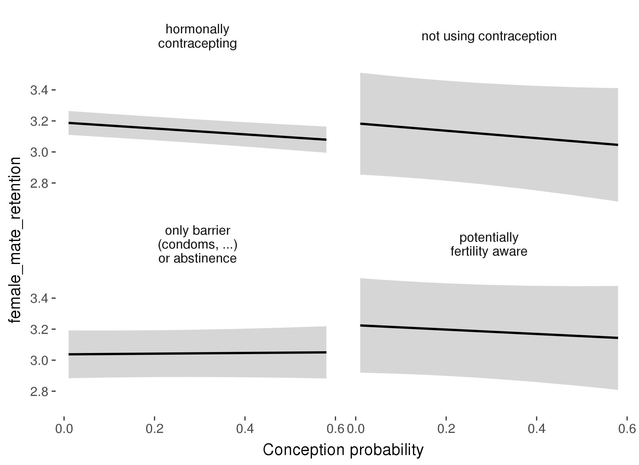

Linear mixed model fit by REML ['lmerMod']
Formula: female_mate_retention ~ fertile_mean + (1 | person) + contraceptive_methods +
fertile + menstruation + fertile:contraceptive_methods + menstruation:contraceptive_methods
Data: diary
Subset: !is.na(included_lax) & contraceptive_method != "other"
REML criterion at convergence: 44329
Scaled residuals:
Min 1Q Median 3Q Max
-4.126 -0.635 -0.008 0.636 4.544
Random effects:
Groups Name Variance Std.Dev.
person (Intercept) 0.533 0.730
Residual 0.716 0.846
Number of obs: 17027, groups: person, 513
Fixed effects:
Estimate Std. Error t value
(Intercept) 3.12885 0.13961 22.41
fertile_mean -0.56419 0.67951 -0.83
contraceptive_methodsfertility_awareness 0.20089 0.18082 1.11
contraceptive_methodsnone 0.20051 0.19163 1.05
contraceptive_methodshormonal 0.17031 0.09119 1.87
fertile 0.02230 0.09443 0.24
menstruationpre -0.02745 0.04561 -0.60
menstruationyes 0.07601 0.04356 1.74
contraceptive_methodsfertility_awareness:fertile -0.16329 0.21445 -0.76
contraceptive_methodsnone:fertile -0.26221 0.23216 -1.13
contraceptive_methodshormonal:fertile -0.21183 0.10550 -2.01
contraceptive_methodsfertility_awareness:menstruationpre -0.04443 0.10102 -0.44
contraceptive_methodsnone:menstruationpre -0.16554 0.10562 -1.57
contraceptive_methodshormonal:menstruationpre -0.00909 0.05137 -0.18
contraceptive_methodsfertility_awareness:menstruationyes -0.02864 0.10153 -0.28
contraceptive_methodsnone:menstruationyes -0.13480 0.11044 -1.22
contraceptive_methodshormonal:menstruationyes -0.10226 0.04968 -2.06
refitting model(s) with ML (instead of REML)
| Df | AIC | BIC | logLik | deviance | Chisq | Chi Df | Pr(>Chisq) | |
|---|---|---|---|---|---|---|---|---|
| add_main | 13 | 44304 | 44405 | -22139 | 44278 | NA | NA | NA |
| by_method | 19 | 44313 | 44460 | -22137 | 44275 | 3.327 | 6 | 0.7668 |
M_m2: Moderation by participant age
model %>%
test_moderator("age_group", diary, xlevels = 5)refitting model(s) with ML (instead of REML)
| Df | AIC | BIC | logLik | deviance | Chisq | Chi Df | Pr(>Chisq) | |
|---|---|---|---|---|---|---|---|---|
| with_main | 19 | 69584 | 69740 | -34773 | 69546 | NA | NA | NA |
| with_mod | 27 | 69594 | 69815 | -34770 | 69540 | 5.948 | 8 | 0.6531 |
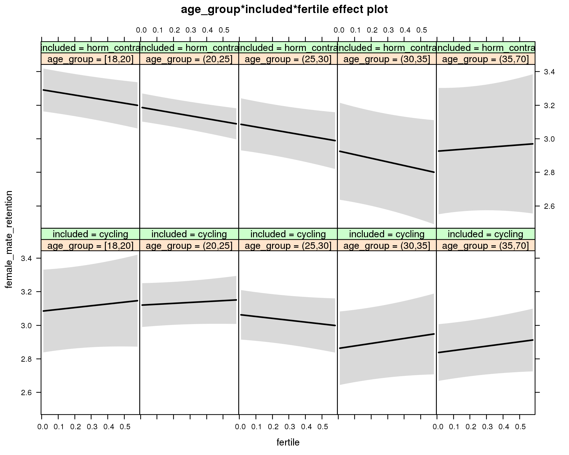
Linear mixed model fit by REML ['lmerMod']
Formula: female_mate_retention ~ menstruation + fertile_mean + (1 | person) +
age_group + included + fertile + menstruation:included +
age_group:included + age_group:fertile + included:fertile + age_group:included:fertile
Data: diary
REML criterion at convergence: 69621
Scaled residuals:
Min 1Q Median 3Q Max
-4.142 -0.628 -0.003 0.632 4.543
Random effects:
Groups Name Variance Std.Dev.
person (Intercept) 0.538 0.734
Residual 0.712 0.844
Number of obs: 26681, groups: person, 1054
Fixed effects:
Estimate Std. Error t value
(Intercept) 3.10554 0.13290 23.37
menstruationpre -0.00859 0.02577 -0.33
menstruationyes 0.01645 0.02429 0.68
fertile_mean -0.13165 0.29073 -0.45
age_group(20,25] 0.03590 0.14241 0.25
age_group(25,30] -0.02052 0.14657 -0.14
age_group(30,35] -0.22179 0.16819 -1.32
age_group(35,70] -0.24737 0.15233 -1.62
includedhorm_contra 0.21847 0.14262 1.53
fertile 0.10772 0.14866 0.72
menstruationpre:includedhorm_contra -0.03437 0.03308 -1.04
menstruationyes:includedhorm_contra -0.02287 0.03185 -0.72
age_group(20,25]:includedhorm_contra -0.14051 0.16245 -0.86
age_group(25,30]:includedhorm_contra -0.18416 0.17888 -1.03
age_group(30,35]:includedhorm_contra -0.14293 0.23300 -0.61
age_group(35,70]:includedhorm_contra -0.11890 0.25396 -0.47
age_group(20,25]:fertile -0.05404 0.16469 -0.33
age_group(25,30]:fertile -0.21904 0.16975 -1.29
age_group(30,35]:fertile 0.04079 0.19663 0.21
age_group(35,70]:fertile 0.02276 0.17742 0.13
includedhorm_contra:fertile -0.26817 0.16488 -1.63
age_group(20,25]:includedhorm_contra:fertile 0.04469 0.18448 0.24
age_group(25,30]:includedhorm_contra:fertile 0.20948 0.20444 1.02
age_group(30,35]:includedhorm_contra:fertile -0.09856 0.26388 -0.37
age_group(35,70]:includedhorm_contra:fertile 0.21292 0.29978 0.71
M_m3: Moderation by weekend
model %>%
test_moderator("weekend", diary, xlevels = 2) refitting model(s) with ML (instead of REML)
| Df | AIC | BIC | logLik | deviance | Chisq | Chi Df | Pr(>Chisq) | |
|---|---|---|---|---|---|---|---|---|
| with_main | 13 | 69293 | 69400 | -34634 | 69267 | NA | NA | NA |
| with_mod | 15 | 69297 | 69419 | -34633 | 69267 | 0.9858 | 2 | 0.6108 |
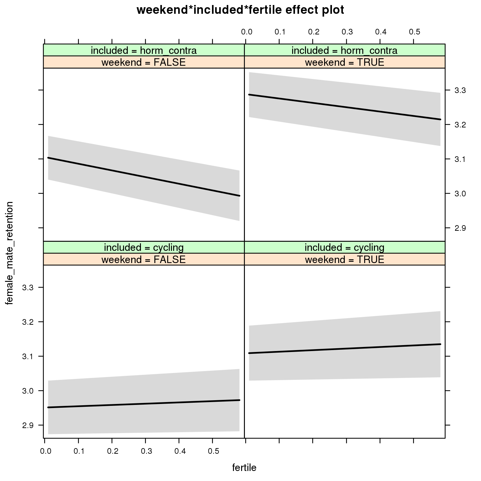
Linear mixed model fit by REML ['lmerMod']
Formula: female_mate_retention ~ menstruation + fertile_mean + (1 | person) +
weekend + included + fertile + menstruation:included + weekend:included +
weekend:fertile + included:fertile + weekend:included:fertile
Data: diary
REML criterion at convergence: 69329
Scaled residuals:
Min 1Q Median 3Q Max
-4.076 -0.624 0.006 0.633 4.639
Random effects:
Groups Name Variance Std.Dev.
person (Intercept) 0.543 0.737
Residual 0.704 0.839
Number of obs: 26681, groups: person, 1054
Fixed effects:
Estimate Std. Error t value
(Intercept) 2.97043 0.06406 46.4
menstruationpre -0.00838 0.02562 -0.3
menstruationyes 0.01657 0.02414 0.7
fertile_mean -0.11944 0.29010 -0.4
weekendTRUE 0.15745 0.02232 7.1
includedhorm_contra 0.16431 0.05327 3.1
fertile 0.03704 0.06288 0.6
menstruationpre:includedhorm_contra -0.03505 0.03289 -1.1
menstruationyes:includedhorm_contra -0.01959 0.03165 -0.6
weekendTRUE:includedhorm_contra 0.02519 0.02873 0.9
weekendTRUE:fertile 0.00849 0.08656 0.1
includedhorm_contra:fertile -0.23076 0.07991 -2.9
weekendTRUE:includedhorm_contra:fertile 0.05872 0.11010 0.5
M_m4: Moderation by weekday
model %>%
test_moderator("weekday", diary, xlevels = 7)refitting model(s) with ML (instead of REML)
| Df | AIC | BIC | logLik | deviance | Chisq | Chi Df | Pr(>Chisq) | |
|---|---|---|---|---|---|---|---|---|
| with_main | 23 | 69106 | 69294 | -34530 | 69060 | NA | NA | NA |
| with_mod | 35 | 69123 | 69410 | -34527 | 69053 | 6.795 | 12 | 0.8708 |
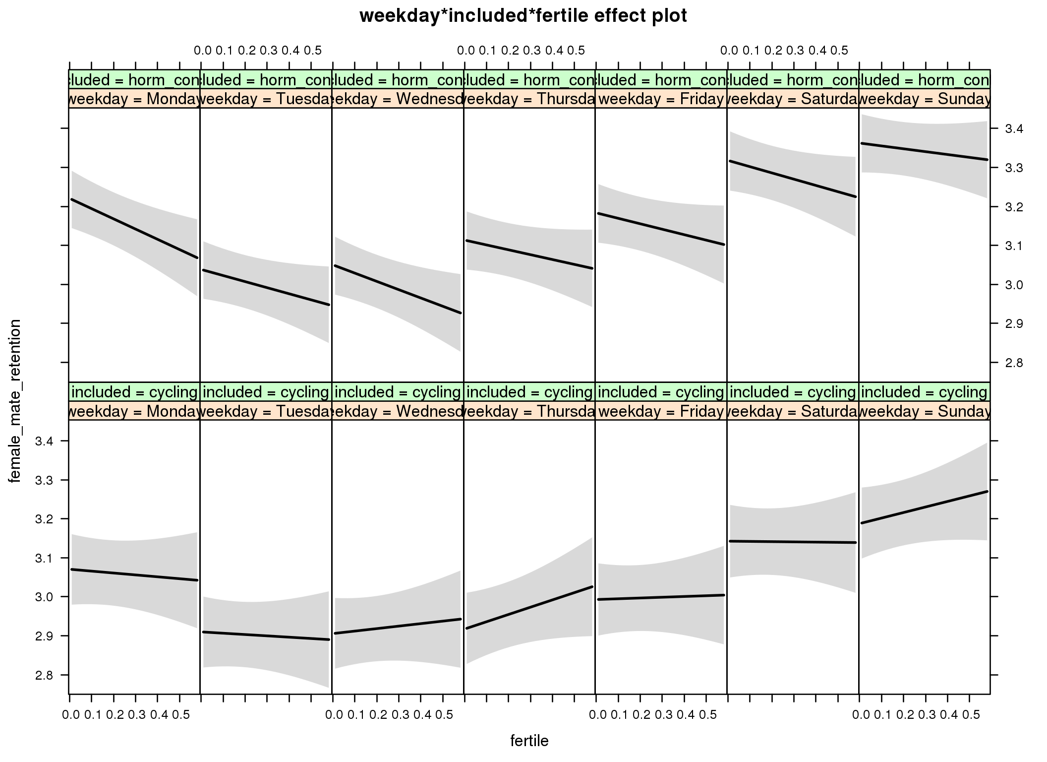
Linear mixed model fit by REML ['lmerMod']
Formula: female_mate_retention ~ menstruation + fertile_mean + (1 | person) +
weekday + included + fertile + menstruation:included + weekday:included +
weekday:fertile + included:fertile + weekday:included:fertile
Data: diary
REML criterion at convergence: 69194
Scaled residuals:
Min 1Q Median 3Q Max
-4.187 -0.624 0.008 0.631 4.635
Random effects:
Groups Name Variance Std.Dev.
person (Intercept) 0.544 0.738
Residual 0.698 0.836
Number of obs: 26681, groups: person, 1054
Fixed effects:
Estimate Std. Error t value
(Intercept) 3.09311 0.06851 45.2
menstruationpre -0.00839 0.02553 -0.3
menstruationyes 0.01601 0.02405 0.7
fertile_mean -0.13709 0.29010 -0.5
weekdayTuesday -0.16078 0.03979 -4.0
weekdayWednesday -0.16509 0.03972 -4.2
weekdayThursday -0.15346 0.04017 -3.8
weekdayFriday -0.07770 0.04085 -1.9
weekdaySaturday 0.07197 0.04126 1.7
weekdaySunday 0.11705 0.03987 2.9
includedhorm_contra 0.15903 0.06164 2.6
fertile -0.04866 0.11207 -0.4
menstruationpre:includedhorm_contra -0.03365 0.03277 -1.0
menstruationyes:includedhorm_contra -0.01742 0.03153 -0.6
weekdayTuesday:includedhorm_contra -0.02160 0.05111 -0.4
weekdayWednesday:includedhorm_contra -0.00541 0.05128 -0.1
weekdayThursday:includedhorm_contra 0.04650 0.05177 0.9
weekdayFriday:includedhorm_contra 0.04056 0.05248 0.8
weekdaySaturday:includedhorm_contra 0.02544 0.05309 0.5
weekdaySunday:includedhorm_contra 0.02491 0.05147 0.5
weekdayTuesday:fertile 0.01470 0.15427 0.1
weekdayWednesday:fertile 0.11253 0.15498 0.7
weekdayThursday:fertile 0.23578 0.15720 1.5
weekdayFriday:fertile 0.06811 0.15747 0.4
weekdaySaturday:fertile 0.04262 0.15957 0.3
weekdaySunday:fertile 0.19085 0.15507 1.2
includedhorm_contra:fertile -0.21383 0.14335 -1.5
weekdayTuesday:includedhorm_contra:fertile 0.09181 0.19689 0.5
weekdayWednesday:includedhorm_contra:fertile -0.06276 0.19844 -0.3
weekdayThursday:includedhorm_contra:fertile -0.09829 0.20007 -0.5
weekdayFriday:includedhorm_contra:fertile 0.05434 0.20066 0.3
weekdaySaturday:includedhorm_contra:fertile 0.05934 0.20355 0.3
weekdaySunday:includedhorm_contra:fertile -0.00195 0.19808 0.0
M_m5: Moderation by exclusion threshold
model %>%
test_moderator("included_levels", diary, xlevels = 4)refitting model(s) with ML (instead of REML)
| Df | AIC | BIC | logLik | deviance | Chisq | Chi Df | Pr(>Chisq) | |
|---|---|---|---|---|---|---|---|---|
| with_main | 17 | 69590 | 69729 | -34778 | 69556 | NA | NA | NA |
| with_mod | 23 | 69594 | 69782 | -34774 | 69548 | 7.624 | 6 | 0.267 |
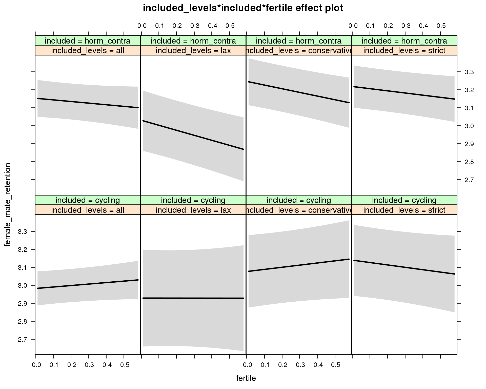
Linear mixed model fit by REML ['lmerMod']
Formula: female_mate_retention ~ menstruation + fertile_mean + (1 | person) +
included_levels + included + fertile + menstruation:included +
included_levels:included + included_levels:fertile + included:fertile +
included_levels:included:fertile
Data: diary
REML criterion at convergence: 69624
Scaled residuals:
Min 1Q Median 3Q Max
-4.168 -0.630 -0.005 0.633 4.536
Random effects:
Groups Name Variance Std.Dev.
person (Intercept) 0.542 0.736
Residual 0.712 0.844
Number of obs: 26681, groups: person, 1054
Fixed effects:
Estimate Std. Error t value
(Intercept) 3.007869 0.070413 42.7
menstruationpre -0.009948 0.025787 -0.4
menstruationyes 0.017375 0.024287 0.7
fertile_mean -0.156817 0.292651 -0.5
included_levelslax -0.053670 0.145703 -0.4
included_levelsconservative 0.094242 0.113672 0.8
included_levelsstrict 0.157491 0.111862 1.4
includedhorm_contra 0.180995 0.072699 2.5
fertile 0.081680 0.065728 1.2
menstruationpre:includedhorm_contra -0.033031 0.033113 -1.0
menstruationyes:includedhorm_contra -0.024149 0.031866 -0.8
included_levelslax:includedhorm_contra -0.068723 0.177239 -0.4
included_levelsconservative:includedhorm_contra -0.000351 0.141872 0.0
included_levelsstrict:includedhorm_contra -0.091914 0.137363 -0.7
included_levelslax:fertile -0.082519 0.160460 -0.5
included_levelsconservative:fertile 0.037010 0.119855 0.3
included_levelsstrict:fertile -0.214496 0.119934 -1.8
includedhorm_contra:fertile -0.171829 0.100452 -1.7
included_levelslax:includedhorm_contra:fertile -0.105983 0.195842 -0.5
included_levelsconservative:includedhorm_contra:fertile -0.150868 0.155883 -1.0
included_levelsstrict:includedhorm_contra:fertile 0.183952 0.153478 1.2
M_m6: Moderation by cycle length
model %>%
test_moderator("cycle_length_groups", diary, xlevels = 4)refitting model(s) with ML (instead of REML)
| Df | AIC | BIC | logLik | deviance | Chisq | Chi Df | Pr(>Chisq) | |
|---|---|---|---|---|---|---|---|---|
| with_main | 17 | 69583 | 69722 | -34775 | 69549 | NA | NA | NA |
| with_mod | 23 | 69589 | 69777 | -34771 | 69543 | 6.111 | 6 | 0.4108 |
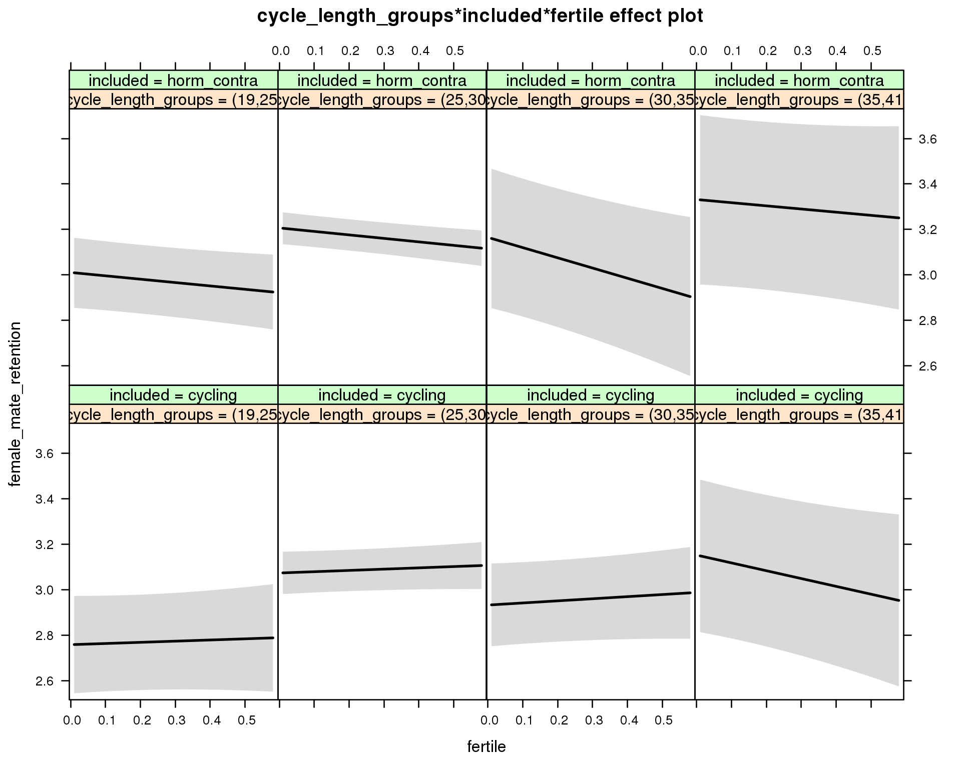
Linear mixed model fit by REML ['lmerMod']
Formula: female_mate_retention ~ menstruation + fertile_mean + (1 | person) +
cycle_length_groups + included + fertile + menstruation:included +
cycle_length_groups:included + cycle_length_groups:fertile +
included:fertile + cycle_length_groups:included:fertile
Data: diary
REML criterion at convergence: 69611
Scaled residuals:
Min 1Q Median 3Q Max
-4.154 -0.629 -0.004 0.633 4.536
Random effects:
Groups Name Variance Std.Dev.
person (Intercept) 0.539 0.734
Residual 0.712 0.844
Number of obs: 26681, groups: person, 1054
Fixed effects:
Estimate Std. Error t value
(Intercept) 2.77382 0.12141 22.85
menstruationpre -0.00713 0.02580 -0.28
menstruationyes 0.01828 0.02446 0.75
fertile_mean -0.10177 0.29323 -0.35
cycle_length_groups(25,30] 0.31542 0.11939 2.64
cycle_length_groups(30,35] 0.17430 0.14369 1.21
cycle_length_groups(35,41] 0.39414 0.20358 1.94
includedhorm_contra 0.26257 0.13566 1.94
fertile 0.05143 0.13724 0.37
menstruationpre:includedhorm_contra -0.03392 0.03311 -1.02
menstruationyes:includedhorm_contra -0.02281 0.03202 -0.71
cycle_length_groups(25,30]:includedhorm_contra -0.11948 0.14744 -0.81
cycle_length_groups(30,35]:includedhorm_contra -0.02020 0.22647 -0.09
cycle_length_groups(35,41]:includedhorm_contra -0.07317 0.28920 -0.25
cycle_length_groups(25,30]:fertile 0.00515 0.14724 0.03
cycle_length_groups(30,35]:fertile 0.04117 0.17433 0.24
cycle_length_groups(35,41]:fertile -0.39529 0.24623 -1.61
includedhorm_contra:fertile -0.19976 0.16201 -1.23
cycle_length_groups(25,30]:includedhorm_contra:fertile -0.01032 0.17444 -0.06
cycle_length_groups(30,35]:includedhorm_contra:fertile -0.34177 0.27447 -1.25
cycle_length_groups(35,41]:includedhorm_contra:fertile 0.40438 0.32424 1.25
M_m7: Moderation by certainty about menstruation parameters
model %>%
test_moderator("certainty_menstruation", diary)refitting model(s) with ML (instead of REML)
| Df | AIC | BIC | logLik | deviance | Chisq | Chi Df | Pr(>Chisq) | |
|---|---|---|---|---|---|---|---|---|
| with_main | 13 | 69587 | 69694 | -34781 | 69561 | NA | NA | NA |
| with_mod | 15 | 69590 | 69713 | -34780 | 69560 | 1.26 | 2 | 0.5325 |
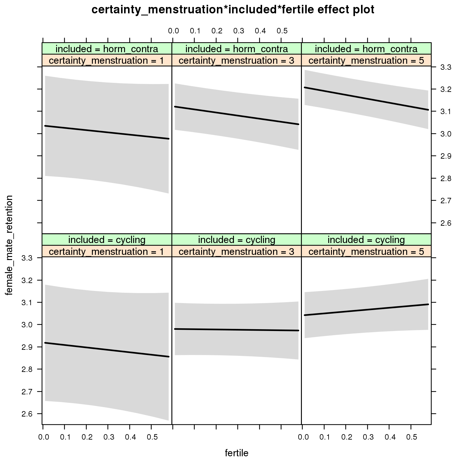
Linear mixed model fit by REML ['lmerMod']
Formula: female_mate_retention ~ menstruation + fertile_mean + (1 | person) +
certainty_menstruation + included + fertile + menstruation:included +
certainty_menstruation:included + certainty_menstruation:fertile +
included:fertile + certainty_menstruation:included:fertile
Data: diary
REML criterion at convergence: 69621
Scaled residuals:
Min 1Q Median 3Q Max
-4.151 -0.628 -0.004 0.630 4.542
Random effects:
Groups Name Variance Std.Dev.
person (Intercept) 0.543 0.737
Residual 0.712 0.844
Number of obs: 26681, groups: person, 1054
Fixed effects:
Estimate Std. Error t value
(Intercept) 2.91333 0.17938 16.24
menstruationpre -0.00757 0.02578 -0.29
menstruationyes 0.01907 0.02431 0.78
fertile_mean -0.15204 0.29087 -0.52
certainty_menstruation 0.03055 0.04090 0.75
includedhorm_contra 0.11406 0.22777 0.50
fertile -0.15764 0.20466 -0.77
menstruationpre:includedhorm_contra -0.03437 0.03309 -1.04
menstruationyes:includedhorm_contra -0.02471 0.03186 -0.78
certainty_menstruation:includedhorm_contra 0.01274 0.05306 0.24
certainty_menstruation:fertile 0.04855 0.04796 1.01
includedhorm_contra:fertile 0.07470 0.26603 0.28
certainty_menstruation:includedhorm_contra:fertile -0.06724 0.06149 -1.09
M_m8: Moderation by cycle regularity
model %>%
test_moderator("cycle_regularity", diary)refitting model(s) with ML (instead of REML)
| Df | AIC | BIC | logLik | deviance | Chisq | Chi Df | Pr(>Chisq) | |
|---|---|---|---|---|---|---|---|---|
| with_main | 15 | 69591 | 69714 | -34780 | 69561 | NA | NA | NA |
| with_mod | 19 | 69593 | 69748 | -34777 | 69555 | 6.027 | 4 | 0.1972 |
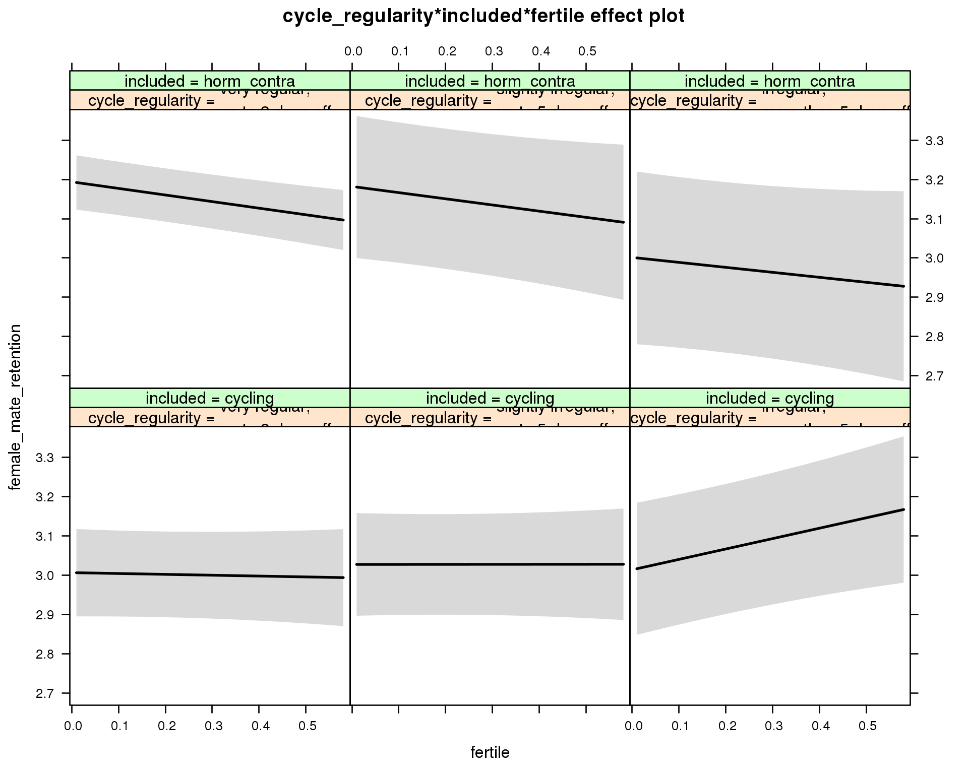
Linear mixed model fit by REML ['lmerMod']
Formula: female_mate_retention ~ menstruation + fertile_mean + (1 | person) +
cycle_regularity + included + fertile + menstruation:included +
cycle_regularity:included + cycle_regularity:fertile + included:fertile +
cycle_regularity:included:fertile
Data: diary
REML criterion at convergence: 69619
Scaled residuals:
Min 1Q Median 3Q Max
-4.149 -0.627 -0.003 0.630 4.531
Random effects:
Groups Name Variance Std.Dev.
person (Intercept) 0.544 0.737
Residual 0.712 0.844
Number of obs: 26681, groups: person, 1054
Fixed effects:
Estimate Std. Error t value
(Intercept) 3.03400 0.07504 40.4
menstruationpre -0.01077 0.02578 -0.4
menstruationyes 0.01590 0.02429 0.7
fertile_mean -0.16227 0.29205 -0.6
cycle_regularityslightly irregular,\nup to 5 days off 0.02096 0.08750 0.2
cycle_regularityirregular,\nmore than 5 days off 0.00732 0.10278 0.1
includedhorm_contra 0.19648 0.06845 2.9
fertile -0.02169 0.07199 -0.3
menstruationpre:includedhorm_contra -0.03140 0.03309 -0.9
menstruationyes:includedhorm_contra -0.02154 0.03184 -0.7
cycle_regularityslightly irregular,\nup to 5 days off:includedhorm_contra -0.03268 0.13222 -0.2
cycle_regularityirregular,\nmore than 5 days off:includedhorm_contra -0.19968 0.15625 -1.3
cycle_regularityslightly irregular,\nup to 5 days off:fertile 0.02235 0.09931 0.2
cycle_regularityirregular,\nmore than 5 days off:fertile 0.28622 0.12215 2.3
includedhorm_contra:fertile -0.14591 0.08435 -1.7
cycle_regularityslightly irregular,\nup to 5 days off:includedhorm_contra:fertile -0.01194 0.14745 -0.1
cycle_regularityirregular,\nmore than 5 days off:includedhorm_contra:fertile -0.24525 0.18233 -1.3
M_m9: Moderation by cohabitation status
model %>%
test_moderator("cohabitation", diary)refitting model(s) with ML (instead of REML)
| Df | AIC | BIC | logLik | deviance | Chisq | Chi Df | Pr(>Chisq) | |
|---|---|---|---|---|---|---|---|---|
| with_main | 15 | 69585 | 69708 | -34777 | 69555 | NA | NA | NA |
| with_mod | 19 | 69592 | 69747 | -34777 | 69554 | 1.271 | 4 | 0.8663 |
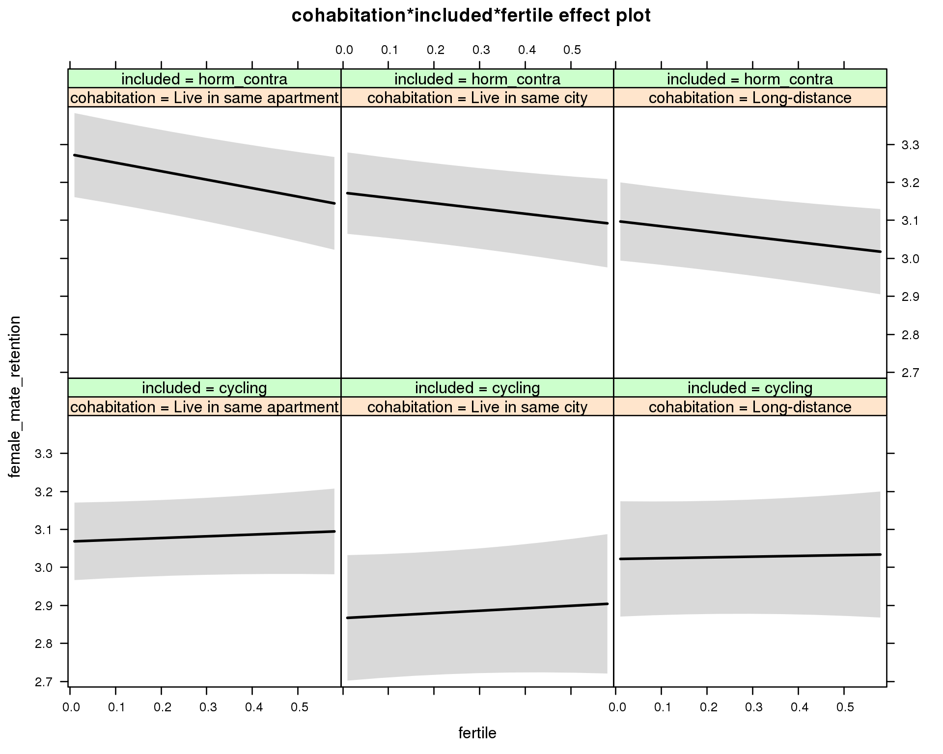
Linear mixed model fit by REML ['lmerMod']
Formula: female_mate_retention ~ menstruation + fertile_mean + (1 | person) +
cohabitation + included + fertile + menstruation:included +
cohabitation:included + cohabitation:fertile + included:fertile + cohabitation:included:fertile
Data: diary
REML criterion at convergence: 69621
Scaled residuals:
Min 1Q Median 3Q Max
-4.130 -0.628 -0.004 0.631 4.534
Random effects:
Groups Name Variance Std.Dev.
person (Intercept) 0.540 0.735
Residual 0.712 0.844
Number of obs: 26681, groups: person, 1054
Fixed effects:
Estimate Std. Error t value
(Intercept) 3.09232 0.07254 42.6
menstruationpre -0.00825 0.02576 -0.3
menstruationyes 0.01808 0.02428 0.7
fertile_mean -0.14887 0.29051 -0.5
cohabitationLive in same city -0.20159 0.09901 -2.0
cohabitationLong-distance -0.04601 0.09327 -0.5
includedhorm_contra 0.21555 0.07814 2.8
fertile 0.04567 0.06500 0.7
menstruationpre:includedhorm_contra -0.03282 0.03308 -1.0
menstruationyes:includedhorm_contra -0.02293 0.03183 -0.7
cohabitationLive in same city:includedhorm_contra 0.10059 0.12652 0.8
cohabitationLong-distance:includedhorm_contra -0.12960 0.12107 -1.1
cohabitationLive in same city:fertile 0.01906 0.11880 0.2
cohabitationLong-distance:fertile -0.02540 0.10699 -0.2
includedhorm_contra:fertile -0.26859 0.09498 -2.8
cohabitationLive in same city:includedhorm_contra:fertile 0.06480 0.14854 0.4
cohabitationLong-distance:includedhorm_contra:fertile 0.10910 0.13780 0.8
M_m10: Moderation by relationship status
model %>%
test_moderator("relationship_status_clean", diary)refitting model(s) with ML (instead of REML)
| Df | AIC | BIC | logLik | deviance | Chisq | Chi Df | Pr(>Chisq) | |
|---|---|---|---|---|---|---|---|---|
| with_main | 15 | 69587 | 69709 | -34778 | 69557 | NA | NA | NA |
| with_mod | 19 | 69592 | 69748 | -34777 | 69554 | 2.686 | 4 | 0.6116 |
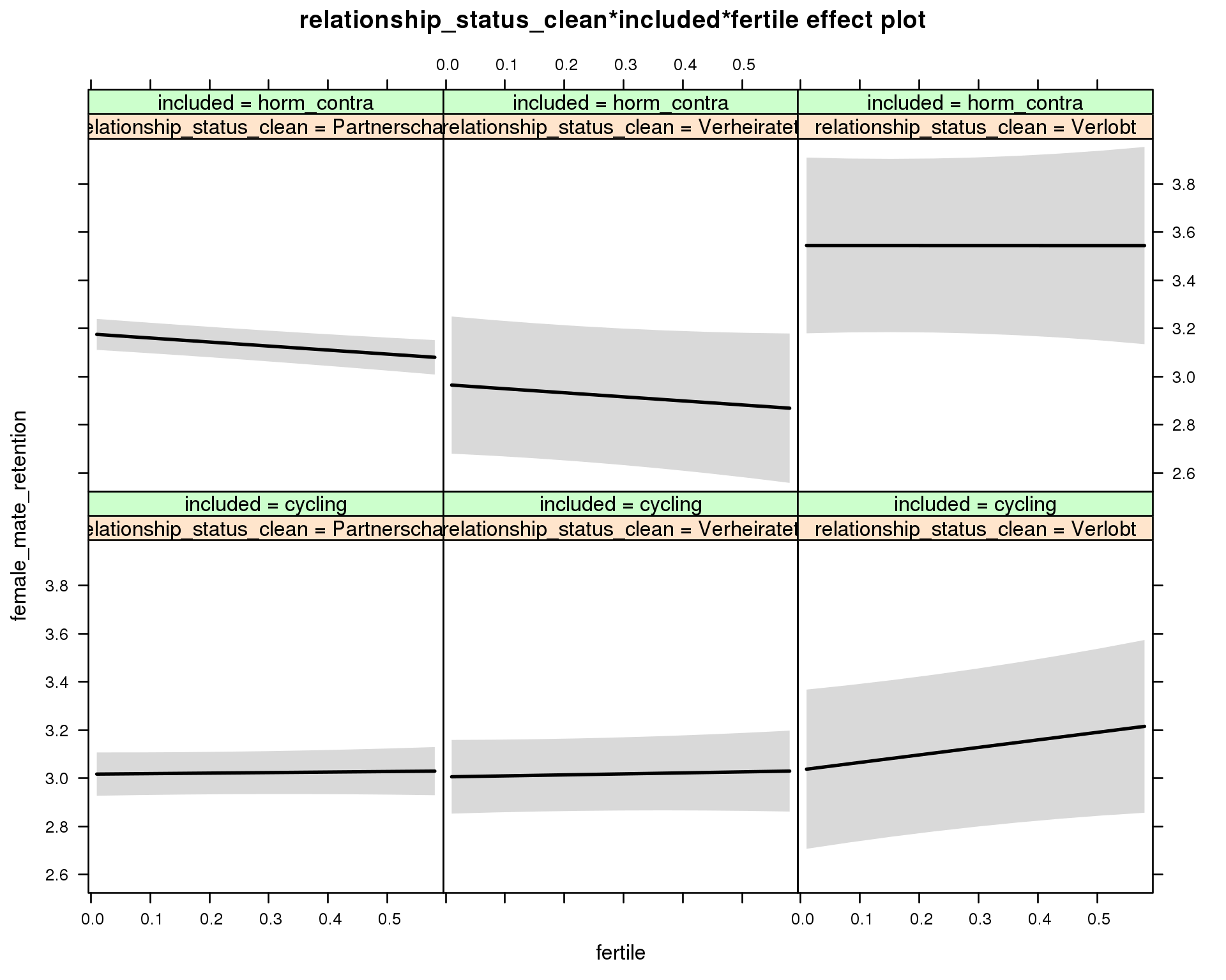
Linear mixed model fit by REML ['lmerMod']
Formula: female_mate_retention ~ menstruation + fertile_mean + (1 | person) +
relationship_status_clean + included + fertile + menstruation:included +
relationship_status_clean:included + relationship_status_clean:fertile +
included:fertile + relationship_status_clean:included:fertile
Data: diary
REML criterion at convergence: 69612
Scaled residuals:
Min 1Q Median 3Q Max
-4.147 -0.627 -0.005 0.631 4.534
Random effects:
Groups Name Variance Std.Dev.
person (Intercept) 0.541 0.735
Residual 0.712 0.844
Number of obs: 26681, groups: person, 1054
Fixed effects:
Estimate Std. Error t value
(Intercept) 3.03418 0.06791 44.7
menstruationpre -0.00826 0.02576 -0.3
menstruationyes 0.01761 0.02428 0.7
fertile_mean -0.10794 0.29035 -0.4
relationship_status_cleanVerheiratet -0.01131 0.09047 -0.1
relationship_status_cleanVerlobt 0.01749 0.17496 0.1
includedhorm_contra 0.16959 0.05827 2.9
fertile 0.02161 0.05954 0.4
menstruationpre:includedhorm_contra -0.03402 0.03308 -1.0
menstruationyes:includedhorm_contra -0.02317 0.03183 -0.7
relationship_status_cleanVerheiratet:includedhorm_contra -0.19910 0.17448 -1.1
relationship_status_cleanVerlobt:includedhorm_contra 0.35006 0.25785 1.4
relationship_status_cleanVerheiratet:fertile 0.01977 0.10482 0.2
relationship_status_cleanVerlobt:fertile 0.29018 0.19659 1.5
includedhorm_contra:fertile -0.18858 0.07259 -2.6
relationship_status_cleanVerheiratet:includedhorm_contra:fertile -0.02098 0.19739 -0.1
relationship_status_cleanVerlobt:includedhorm_contra:fertile -0.12410 0.30530 -0.4
do_moderators(models$female_mate_retention, diary)Moderators
Partner’s physical attractiveness
Predicted fertile phase effect sizes (in red): biggest (EP desire, partner mate retention)/smallest (IP desire) when partner’s physical attractiveness is low.
model %>%
test_moderator("partner_attractiveness_physical", diary)refitting model(s) with ML (instead of REML)
| Df | AIC | BIC | logLik | deviance | Chisq | Chi Df | Pr(>Chisq) | |
|---|---|---|---|---|---|---|---|---|
| with_main | 13 | 69538 | 69644 | -34756 | 69512 | NA | NA | NA |
| with_mod | 15 | 69540 | 69663 | -34755 | 69510 | 1.197 | 2 | 0.5496 |
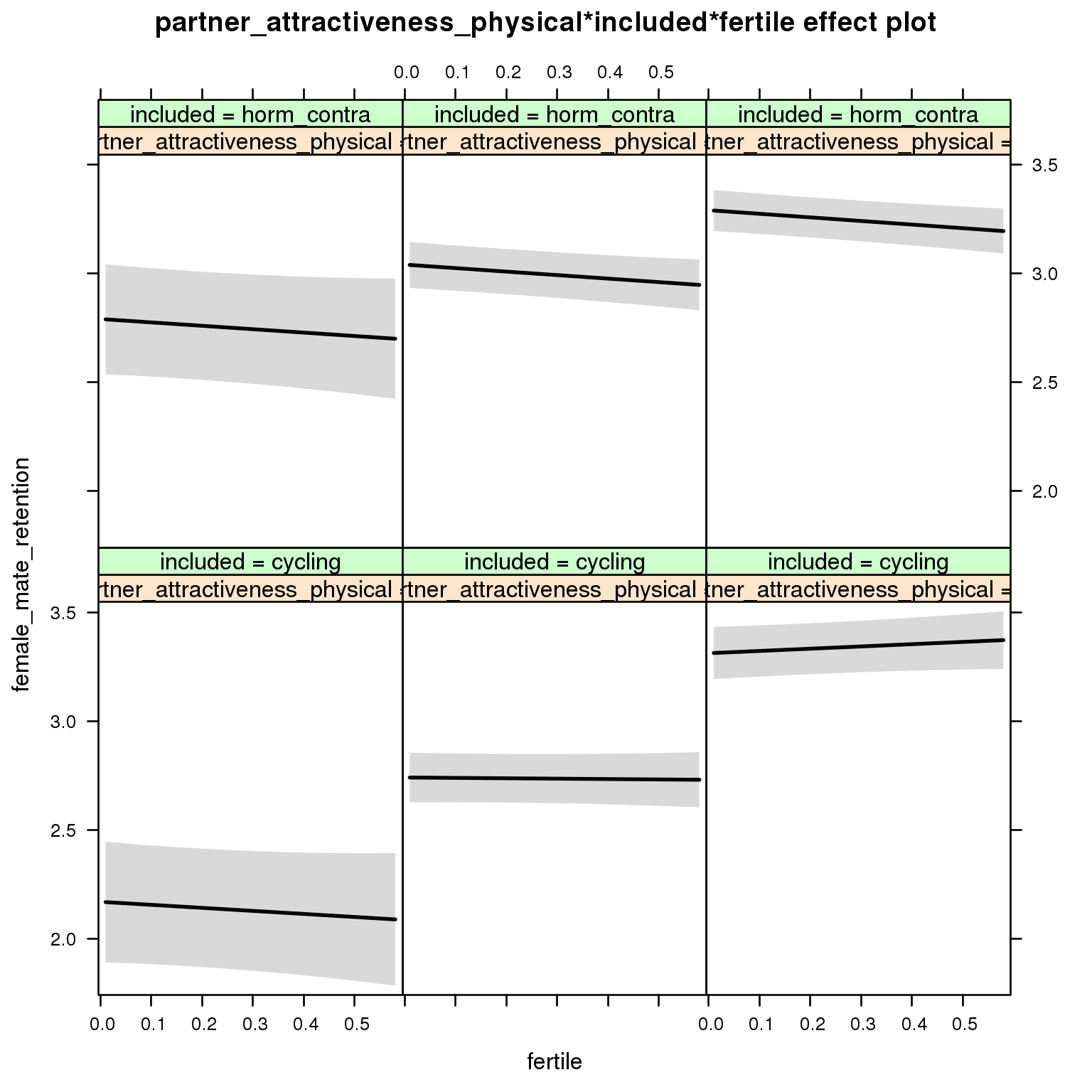
Linear mixed model fit by REML ['lmerMod']
Formula: female_mate_retention ~ menstruation + fertile_mean + (1 | person) +
partner_attractiveness_physical + included + fertile + menstruation:included +
partner_attractiveness_physical:included + partner_attractiveness_physical:fertile +
included:fertile + partner_attractiveness_physical:included:fertile
Data: diary
REML criterion at convergence: 69576
Scaled residuals:
Min 1Q Median 3Q Max
-4.151 -0.628 -0.003 0.632 4.532
Random effects:
Groups Name Variance Std.Dev.
person (Intercept) 0.517 0.719
Residual 0.712 0.844
Number of obs: 26681, groups: person, 1054
Fixed effects:
Estimate Std. Error t value
(Intercept) 1.91172 0.19248 9.93
menstruationpre -0.00921 0.02576 -0.36
menstruationyes 0.01717 0.02428 0.71
fertile_mean -0.16521 0.28511 -0.58
partner_attractiveness_physical 0.14279 0.02308 6.19
includedhorm_contra 0.79151 0.25185 3.14
fertile -0.20025 0.22693 -0.88
menstruationpre:includedhorm_contra -0.03299 0.03307 -1.00
menstruationyes:includedhorm_contra -0.02294 0.03183 -0.72
partner_attractiveness_physical:includedhorm_contra -0.08029 0.03071 -2.61
partner_attractiveness_physical:fertile 0.03040 0.02781 1.09
includedhorm_contra:fertile 0.04619 0.30021 0.15
partner_attractiveness_physical:includedhorm_contra:fertile -0.03153 0.03630 -0.87
Partner’s short-term attractiveness
Predicted fertile phase effect sizes (in red): biggest (EP desire, partner mate retention)/smallest (IP desire) when partner’s short-term attractiveness is low.
model %>%
test_moderator("partner_attractiveness_shortterm", diary)refitting model(s) with ML (instead of REML)
| Df | AIC | BIC | logLik | deviance | Chisq | Chi Df | Pr(>Chisq) | |
|---|---|---|---|---|---|---|---|---|
| with_main | 13 | 69550 | 69656 | -34762 | 69524 | NA | NA | NA |
| with_mod | 15 | 69553 | 69676 | -34762 | 69523 | 0.379 | 2 | 0.8274 |
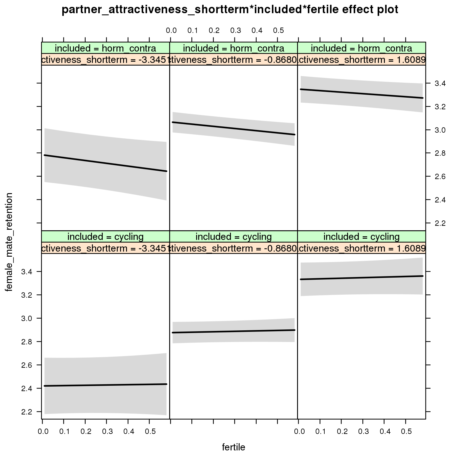
Linear mixed model fit by REML ['lmerMod']
Formula: female_mate_retention ~ menstruation + fertile_mean + (1 | person) +
partner_attractiveness_shortterm + included + fertile + menstruation:included +
partner_attractiveness_shortterm:included + partner_attractiveness_shortterm:fertile +
included:fertile + partner_attractiveness_shortterm:included:fertile
Data: diary
REML criterion at convergence: 69586
Scaled residuals:
Min 1Q Median 3Q Max
-4.168 -0.627 -0.004 0.631 4.523
Random effects:
Groups Name Variance Std.Dev.
person (Intercept) 0.523 0.723
Residual 0.712 0.844
Number of obs: 26681, groups: person, 1054
Fixed effects:
Estimate Std. Error t value
(Intercept) 3.06292 0.06273 48.8
menstruationpre -0.00892 0.02576 -0.3
menstruationyes 0.01696 0.02428 0.7
fertile_mean -0.15953 0.28636 -0.6
partner_attractiveness_shortterm 0.18442 0.03642 5.1
includedhorm_contra 0.13815 0.05154 2.7
fertile 0.04215 0.05218 0.8
menstruationpre:includedhorm_contra -0.03339 0.03307 -1.0
menstruationyes:includedhorm_contra -0.02277 0.03183 -0.7
partner_attractiveness_shortterm:includedhorm_contra -0.07060 0.04908 -1.4
partner_attractiveness_shortterm:fertile 0.00471 0.04368 0.1
includedhorm_contra:fertile -0.20875 0.06625 -3.2
partner_attractiveness_shortterm:includedhorm_contra:fertile 0.01771 0.05723 0.3
Partner’s short-term vs. long-term attractiveness
Predicted fertile phase effect sizes (in red): biggest (EP desire, partner mate retention)/smallest (IP desire) top-right (high LT, low ST), then top-left (low LT, low ST), then bottom-left (low LT, high ST), then bottom-right (high LT/ST).
add_main = update.formula(formula(model), new = as.formula(paste0(". ~ . + partner_attractiveness_longterm * included + partner_attractiveness_shortterm * included + partner_attractiveness_longterm * partner_attractiveness_shortterm"))) # reorder so that the triptych looks nice
add_mod_formula = update.formula(update.formula(formula(model), new = . ~ . - included * fertile), new = as.formula(paste0(". ~ . + partner_attractiveness_longterm * fertile * partner_attractiveness_shortterm * included"))) # reorder so that the triptych looks nice
update(model, formula = add_main) -> with_main
update(model, formula = add_mod_formula) -> with_mod
cat(pander(anova(with_main, with_mod)))refitting model(s) with ML (instead of REML)
| Df | AIC | BIC | logLik | deviance | Chisq | Chi Df | Pr(>Chisq) | |
|---|---|---|---|---|---|---|---|---|
| with_main | 16 | 69492 | 69623 | -34730 | 69460 | NA | NA | NA |
| with_mod | 23 | 69496 | 69685 | -34725 | 69450 | 9.696 | 7 | 0.2065 |
effs = allEffects(with_mod)
effs = data.frame(effs$`partner_attractiveness_longterm:fertile:partner_attractiveness_shortterm:included`) %>%
filter(partner_attractiveness_longterm %in% c(-2,0),partner_attractiveness_shortterm %in% c(-2,0))
ggplot(effs, aes(fertile, fit, ymin = lower, ymax = upper, color = included)) +
facet_grid(partner_attractiveness_shortterm ~ partner_attractiveness_longterm) +
geom_smooth(stat='identity') +
scale_color_manual(values = c("cycling" = 'red', 'horm_contra' = 'black'), guide = F) +
scale_fill_manual(values = c("cycling" = 'red', 'horm_contra' = 'black'), guide = F) +
ggtitle("Moderation", "top-to-bottom: short-term,\nleft-to-right: long-term attractiveness of the partner")+
ylab(names(model@frame)[1])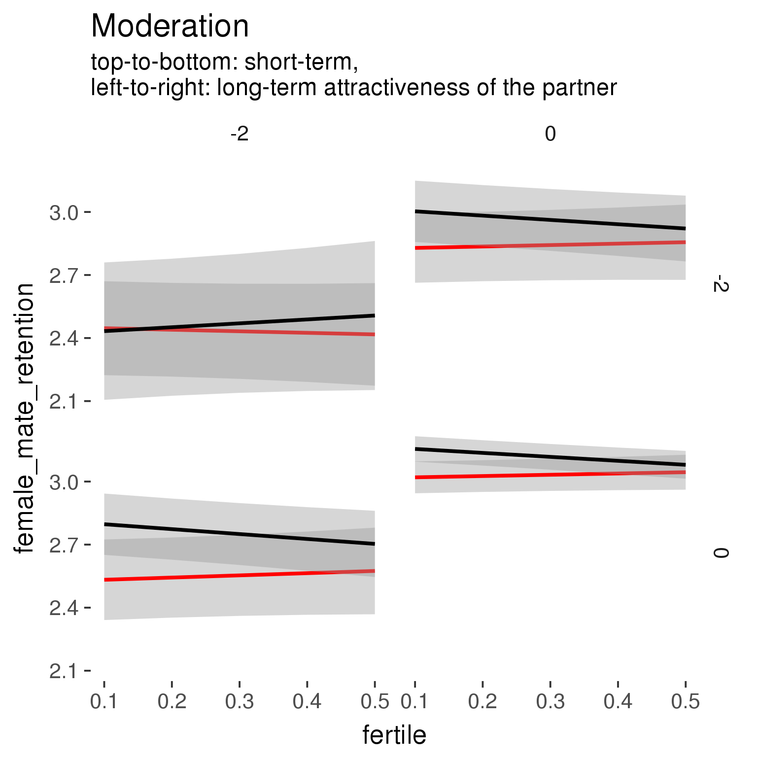
print_summary(with_mod)Linear mixed model fit by REML ['lmerMod']
Formula: female_mate_retention ~ menstruation + fertile_mean + (1 | person) +
partner_attractiveness_longterm + fertile + partner_attractiveness_shortterm +
included + menstruation:included + partner_attractiveness_longterm:fertile +
partner_attractiveness_longterm:partner_attractiveness_shortterm +
fertile:partner_attractiveness_shortterm + partner_attractiveness_longterm:included +
fertile:included + partner_attractiveness_shortterm:included +
partner_attractiveness_longterm:fertile:partner_attractiveness_shortterm +
partner_attractiveness_longterm:fertile:included + partner_attractiveness_longterm:partner_attractiveness_shortterm:included +
fertile:partner_attractiveness_shortterm:included + partner_attractiveness_longterm:fertile:partner_attractiveness_shortterm:included
Data: diary
REML criterion at convergence: 69550
Scaled residuals:
Min 1Q Median 3Q Max
-4.209 -0.627 -0.004 0.631 4.573
Random effects:
Groups Name Variance Std.Dev.
person (Intercept) 0.491 0.701
Residual 0.712 0.844
Number of obs: 26681, groups: person, 1054
Fixed effects:
Estimate
(Intercept) 3.02452
menstruationpre -0.00893
menstruationyes 0.01735
fertile_mean -0.06836
partner_attractiveness_longterm 0.24593
fertile 0.06087
partner_attractiveness_shortterm 0.09599
includedhorm_contra 0.16986
menstruationpre:includedhorm_contra -0.03281
menstruationyes:includedhorm_contra -0.02282
partner_attractiveness_longterm:fertile -0.02201
partner_attractiveness_longterm:partner_attractiveness_shortterm 0.03101
fertile:partner_attractiveness_shortterm -0.00350
partner_attractiveness_longterm:includedhorm_contra -0.06907
fertile:includedhorm_contra -0.24955
partner_attractiveness_shortterm:includedhorm_contra -0.02066
partner_attractiveness_longterm:fertile:partner_attractiveness_shortterm -0.04646
partner_attractiveness_longterm:fertile:includedhorm_contra 0.04472
partner_attractiveness_longterm:partner_attractiveness_shortterm:includedhorm_contra -0.09487
fertile:partner_attractiveness_shortterm:includedhorm_contra 0.01153
partner_attractiveness_longterm:fertile:partner_attractiveness_shortterm:includedhorm_contra 0.15545
Std. Error
(Intercept) 0.06280
menstruationpre 0.02576
menstruationyes 0.02430
fertile_mean 0.28008
partner_attractiveness_longterm 0.04286
fertile 0.05442
partner_attractiveness_shortterm 0.03947
includedhorm_contra 0.05259
menstruationpre:includedhorm_contra 0.03307
menstruationyes:includedhorm_contra 0.03184
partner_attractiveness_longterm:fertile 0.05260
partner_attractiveness_longterm:partner_attractiveness_shortterm 0.03155
fertile:partner_attractiveness_shortterm 0.04769
partner_attractiveness_longterm:includedhorm_contra 0.05464
fertile:includedhorm_contra 0.06859
partner_attractiveness_shortterm:includedhorm_contra 0.05145
partner_attractiveness_longterm:fertile:partner_attractiveness_shortterm 0.03896
partner_attractiveness_longterm:fertile:includedhorm_contra 0.06671
partner_attractiveness_longterm:partner_attractiveness_shortterm:includedhorm_contra 0.04924
fertile:partner_attractiveness_shortterm:includedhorm_contra 0.06114
partner_attractiveness_longterm:fertile:partner_attractiveness_shortterm:includedhorm_contra 0.06033
t value
(Intercept) 48.2
menstruationpre -0.3
menstruationyes 0.7
fertile_mean -0.2
partner_attractiveness_longterm 5.7
fertile 1.1
partner_attractiveness_shortterm 2.4
includedhorm_contra 3.2
menstruationpre:includedhorm_contra -1.0
menstruationyes:includedhorm_contra -0.7
partner_attractiveness_longterm:fertile -0.4
partner_attractiveness_longterm:partner_attractiveness_shortterm 1.0
fertile:partner_attractiveness_shortterm -0.1
partner_attractiveness_longterm:includedhorm_contra -1.3
fertile:includedhorm_contra -3.6
partner_attractiveness_shortterm:includedhorm_contra -0.4
partner_attractiveness_longterm:fertile:partner_attractiveness_shortterm -1.2
partner_attractiveness_longterm:fertile:includedhorm_contra 0.7
partner_attractiveness_longterm:partner_attractiveness_shortterm:includedhorm_contra -1.9
fertile:partner_attractiveness_shortterm:includedhorm_contra 0.2
partner_attractiveness_longterm:fertile:partner_attractiveness_shortterm:includedhorm_contra 2.6
Relative attractiveness to self
whole MV and MV_P scale
Predicted fertile phase effect sizes (in red): biggest (EP desire, partner mate retention)/smallest (IP desire) when partner’s relative attractiveness is low.
three item subsets of the MV/MV_P scale
model %>%
test_moderator("partner_attractiveness_rel_to_self_MV_short", diary)refitting model(s) with ML (instead of REML)
| Df | AIC | BIC | logLik | deviance | Chisq | Chi Df | Pr(>Chisq) | |
|---|---|---|---|---|---|---|---|---|
| with_main | 13 | 69590 | 69696 | -34782 | 69564 | NA | NA | NA |
| with_mod | 15 | 69593 | 69716 | -34781 | 69563 | 0.6447 | 2 | 0.7244 |
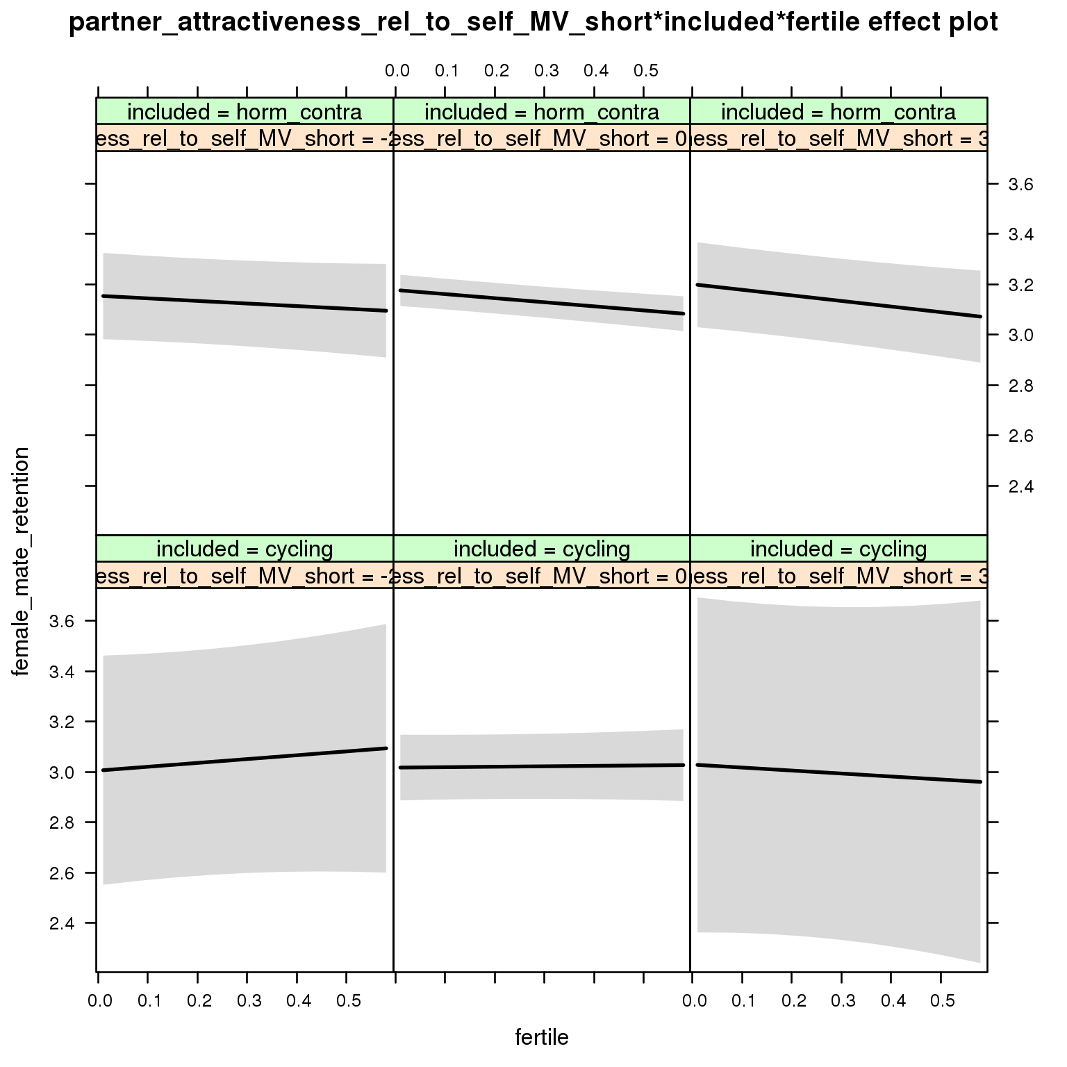
Linear mixed model fit by REML ['lmerMod']
Formula: female_mate_retention ~ menstruation + fertile_mean + (1 | person) +
partner_attractiveness_rel_to_self_MV_short + included +
fertile + menstruation:included + partner_attractiveness_rel_to_self_MV_short:included +
partner_attractiveness_rel_to_self_MV_short:fertile + included:fertile +
partner_attractiveness_rel_to_self_MV_short:included:fertile
Data: diary
REML criterion at convergence: 69622
Scaled residuals:
Min 1Q Median 3Q Max
-4.145 -0.627 -0.003 0.631 4.537
Random effects:
Groups Name Variance Std.Dev.
person (Intercept) 0.544 0.737
Residual 0.712 0.844
Number of obs: 26681, groups: person, 1054
Fixed effects:
Estimate Std. Error t value
(Intercept) 3.03737 0.07141 42.5
menstruationpre -0.00851 0.02576 -0.3
menstruationyes 0.01746 0.02429 0.7
fertile_mean -0.13017 0.29073 -0.4
partner_attractiveness_rel_to_self_MV_short 0.00381 0.09057 0.0
includedhorm_contra 0.16863 0.06112 2.8
fertile 0.02814 0.06181 0.5
menstruationpre:includedhorm_contra -0.03338 0.03308 -1.0
menstruationyes:includedhorm_contra -0.02255 0.03184 -0.7
partner_attractiveness_rel_to_self_MV_short:includedhorm_contra 0.00352 0.09418 0.0
partner_attractiveness_rel_to_self_MV_short:fertile -0.04324 0.10046 -0.4
includedhorm_contra:fertile -0.18533 0.07439 -2.5
partner_attractiveness_rel_to_self_MV_short:includedhorm_contra:fertile 0.02418 0.10434 0.2
model %>%
test_moderator("partner_attractiveness_rel_to_self", diary)refitting model(s) with ML (instead of REML)
| Df | AIC | BIC | logLik | deviance | Chisq | Chi Df | Pr(>Chisq) | |
|---|---|---|---|---|---|---|---|---|
| with_main | 13 | 69590 | 69696 | -34782 | 69564 | NA | NA | NA |
| with_mod | 15 | 69593 | 69716 | -34782 | 69563 | 0.2878 | 2 | 0.866 |
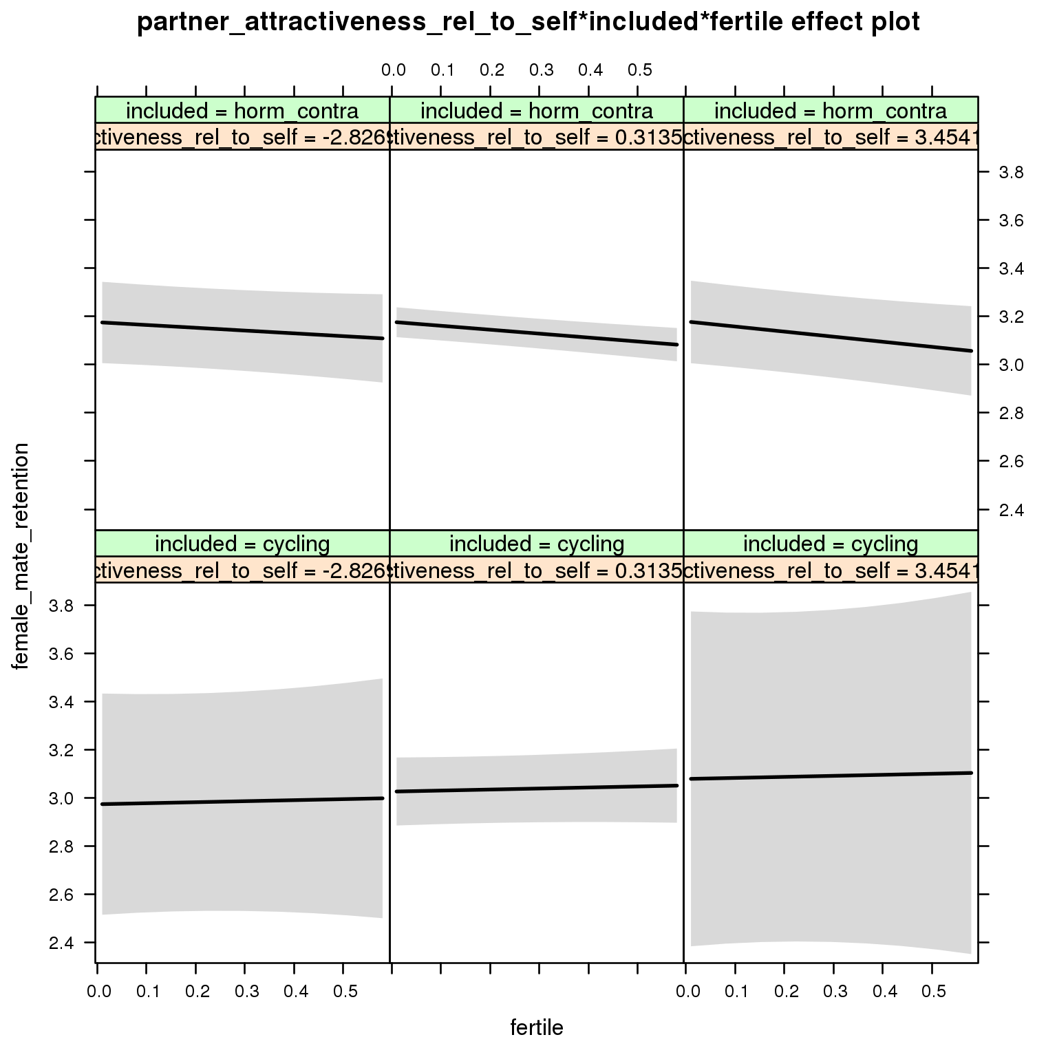
Linear mixed model fit by REML ['lmerMod']
Formula: female_mate_retention ~ menstruation + fertile_mean + (1 | person) +
partner_attractiveness_rel_to_self + included + fertile +
menstruation:included + partner_attractiveness_rel_to_self:included +
partner_attractiveness_rel_to_self:fertile + included:fertile +
partner_attractiveness_rel_to_self:included:fertile
Data: diary
REML criterion at convergence: 69623
Scaled residuals:
Min 1Q Median 3Q Max
-4.145 -0.628 -0.004 0.631 4.538
Random effects:
Groups Name Variance Std.Dev.
person (Intercept) 0.544 0.737
Residual 0.712 0.844
Number of obs: 26681, groups: person, 1054
Fixed effects:
Estimate Std. Error t value
(Intercept) 3.041916 0.071545 42.5
menstruationpre -0.008458 0.025764 -0.3
menstruationyes 0.017733 0.024288 0.7
fertile_mean -0.131477 0.290734 -0.5
partner_attractiveness_rel_to_self 0.016696 0.092996 0.2
includedhorm_contra 0.166276 0.061333 2.7
fertile 0.042590 0.062249 0.7
menstruationpre:includedhorm_contra -0.033473 0.033077 -1.0
menstruationyes:includedhorm_contra -0.022921 0.031837 -0.7
partner_attractiveness_rel_to_self:includedhorm_contra -0.016221 0.096490 -0.2
partner_attractiveness_rel_to_self:fertile 0.000105 0.104041 0.0
includedhorm_contra:fertile -0.200965 0.074765 -2.7
partner_attractiveness_rel_to_self:includedhorm_contra:fertile -0.015195 0.107783 -0.1
Partner’s shortterm attractiveness, alternative specification
model %>%
test_moderator("partner_attractiveness_shortterm_v2", diary)refitting model(s) with ML (instead of REML)
| Df | AIC | BIC | logLik | deviance | Chisq | Chi Df | Pr(>Chisq) | |
|---|---|---|---|---|---|---|---|---|
| with_main | 13 | 69557 | 69663 | -34765 | 69531 | NA | NA | NA |
| with_mod | 15 | 69561 | 69684 | -34765 | 69531 | 0.2636 | 2 | 0.8765 |
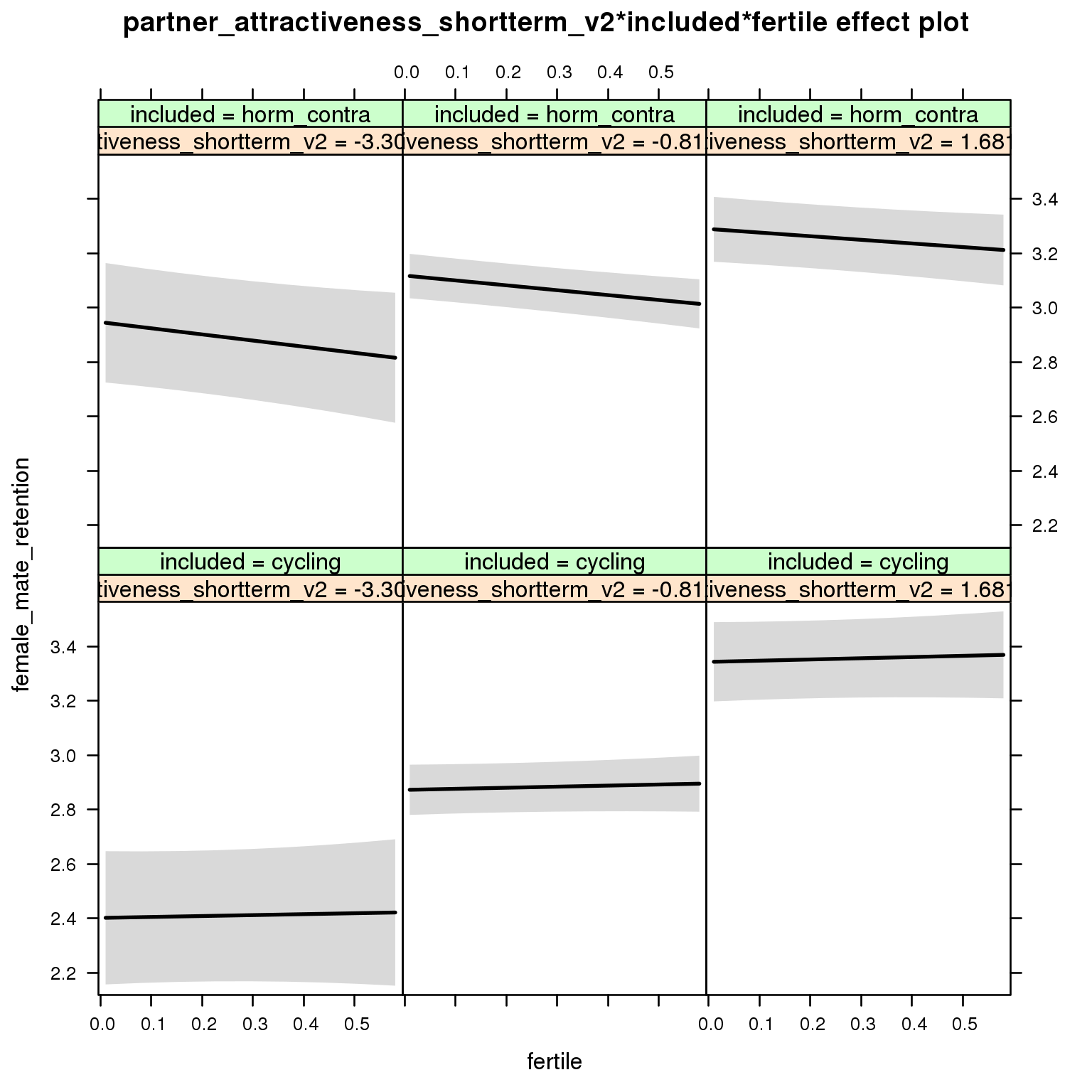
Linear mixed model fit by REML ['lmerMod']
Formula: female_mate_retention ~ menstruation + fertile_mean + (1 | person) +
partner_attractiveness_shortterm_v2 + included + fertile +
menstruation:included + partner_attractiveness_shortterm_v2:included +
partner_attractiveness_shortterm_v2:fertile + included:fertile +
partner_attractiveness_shortterm_v2:included:fertile
Data: diary
REML criterion at convergence: 69593
Scaled residuals:
Min 1Q Median 3Q Max
-4.164 -0.627 -0.003 0.631 4.526
Random effects:
Groups Name Variance Std.Dev.
person (Intercept) 0.527 0.726
Residual 0.712 0.844
Number of obs: 26681, groups: person, 1054
Fixed effects:
Estimate Std. Error t value
(Intercept) 3.05506 0.06282 48.6
menstruationpre -0.00936 0.02576 -0.4
menstruationyes 0.01653 0.02428 0.7
fertile_mean -0.17332 0.28730 -0.6
partner_attractiveness_shortterm_v2 0.18894 0.03678 5.1
includedhorm_contra 0.15760 0.05147 3.1
fertile 0.04114 0.05202 0.8
menstruationpre:includedhorm_contra -0.03287 0.03307 -1.0
menstruationyes:includedhorm_contra -0.02227 0.03183 -0.7
partner_attractiveness_shortterm_v2:includedhorm_contra -0.12014 0.04885 -2.5
partner_attractiveness_shortterm_v2:fertile 0.00205 0.04350 0.0
includedhorm_contra:fertile -0.20570 0.06596 -3.1
partner_attractiveness_shortterm_v2:includedhorm_contra:fertile 0.01646 0.05660 0.3
Partner’s global attractiveness
model %>%
test_moderator("partner_attractiveness_global", diary)refitting model(s) with ML (instead of REML)
| Df | AIC | BIC | logLik | deviance | Chisq | Chi Df | Pr(>Chisq) | |
|---|---|---|---|---|---|---|---|---|
| with_main | 13 | 69583 | 69690 | -34779 | 69557 | NA | NA | NA |
| with_mod | 15 | 69585 | 69707 | -34777 | 69555 | 2.825 | 2 | 0.2436 |
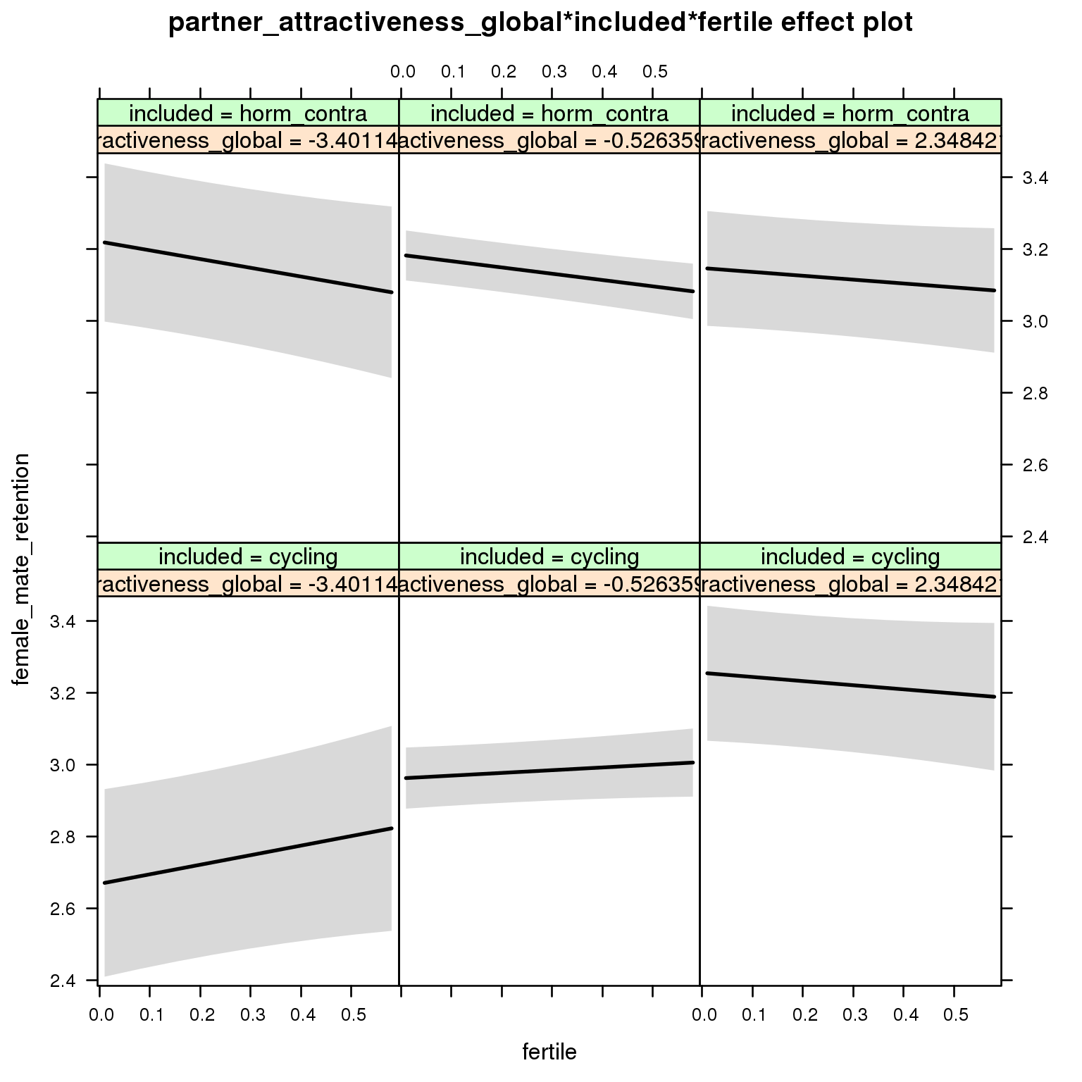
Linear mixed model fit by REML ['lmerMod']
Formula: female_mate_retention ~ menstruation + fertile_mean + (1 | person) +
partner_attractiveness_global + included + fertile + menstruation:included +
partner_attractiveness_global:included + partner_attractiveness_global:fertile +
included:fertile + partner_attractiveness_global:included:fertile
Data: diary
REML criterion at convergence: 69617
Scaled residuals:
Min 1Q Median 3Q Max
-4.160 -0.627 -0.003 0.630 4.528
Random effects:
Groups Name Variance Std.Dev.
person (Intercept) 0.541 0.735
Residual 0.712 0.844
Number of obs: 26681, groups: person, 1054
Fixed effects:
Estimate Std. Error t value
(Intercept) 3.03853 0.06338 47.9
menstruationpre -0.00894 0.02576 -0.3
menstruationyes 0.01706 0.02428 0.7
fertile_mean -0.14408 0.29017 -0.5
partner_attractiveness_global 0.10217 0.03752 2.7
includedhorm_contra 0.17198 0.05192 3.3
fertile 0.04088 0.05199 0.8
menstruationpre:includedhorm_contra -0.03325 0.03308 -1.0
menstruationyes:includedhorm_contra -0.02255 0.03183 -0.7
partner_attractiveness_global:includedhorm_contra -0.11498 0.04924 -2.3
partner_attractiveness_global:fertile -0.06627 0.04311 -1.5
includedhorm_contra:fertile -0.20375 0.06588 -3.1
partner_attractiveness_global:includedhorm_contra:fertile 0.08990 0.05540 1.6
Partner’s longterm attractiveness
model %>%
test_moderator("partner_attractiveness_longterm", diary)refitting model(s) with ML (instead of REML)
| Df | AIC | BIC | logLik | deviance | Chisq | Chi Df | Pr(>Chisq) | |
|---|---|---|---|---|---|---|---|---|
| with_main | 13 | 69497 | 69604 | -34736 | 69471 | NA | NA | NA |
| with_mod | 15 | 69501 | 69624 | -34735 | 69471 | 0.3241 | 2 | 0.8504 |

Linear mixed model fit by REML ['lmerMod']
Formula: female_mate_retention ~ menstruation + fertile_mean + (1 | person) +
partner_attractiveness_longterm + included + fertile + menstruation:included +
partner_attractiveness_longterm:included + partner_attractiveness_longterm:fertile +
included:fertile + partner_attractiveness_longterm:included:fertile
Data: diary
REML criterion at convergence: 69533
Scaled residuals:
Min 1Q Median 3Q Max
-4.157 -0.630 -0.004 0.631 4.555
Random effects:
Groups Name Variance Std.Dev.
person (Intercept) 0.496 0.704
Residual 0.712 0.844
Number of obs: 26681, groups: person, 1054
Fixed effects:
Estimate Std. Error t value
(Intercept) 3.0221401 0.0612476 49.3
menstruationpre -0.0093041 0.0257575 -0.4
menstruationyes 0.0169538 0.0242930 0.7
fertile_mean -0.0395791 0.2808398 -0.1
partner_attractiveness_longterm 0.2706685 0.0368020 7.4
includedhorm_contra 0.1610066 0.0501722 3.2
fertile 0.0426155 0.0519922 0.8
menstruationpre:includedhorm_contra -0.0326821 0.0330668 -1.0
menstruationyes:includedhorm_contra -0.0222080 0.0318348 -0.7
partner_attractiveness_longterm:includedhorm_contra -0.0729381 0.0494322 -1.5
partner_attractiveness_longterm:fertile -0.0000796 0.0460683 0.0
includedhorm_contra:fertile -0.2083287 0.0659408 -3.2
partner_attractiveness_longterm:includedhorm_contra:fertile 0.0228037 0.0609405 0.4
Partner’s short-term vs. long-term attractiveness
We also test this specification of the short-term vs. long-term moderator prediction, but we think this is a suboptimal way to test it.
model %>%
test_moderator("partner_st_vs_lt", diary)refitting model(s) with ML (instead of REML)
| Df | AIC | BIC | logLik | deviance | Chisq | Chi Df | Pr(>Chisq) | |
|---|---|---|---|---|---|---|---|---|
| with_main | 13 | 69583 | 69689 | -34778 | 69557 | NA | NA | NA |
| with_mod | 15 | 69587 | 69710 | -34778 | 69557 | 0.009146 | 2 | 0.9954 |

Linear mixed model fit by REML ['lmerMod']
Formula: female_mate_retention ~ menstruation + fertile_mean + (1 | person) +
partner_st_vs_lt + included + fertile + menstruation:included +
partner_st_vs_lt:included + partner_st_vs_lt:fertile + included:fertile +
partner_st_vs_lt:included:fertile
Data: diary
REML criterion at convergence: 69620
Scaled residuals:
Min 1Q Median 3Q Max
-4.148 -0.627 -0.004 0.631 4.547
Random effects:
Groups Name Variance Std.Dev.
person (Intercept) 0.540 0.735
Residual 0.712 0.844
Number of obs: 26681, groups: person, 1054
Fixed effects:
Estimate Std. Error t value
(Intercept) 3.023442 0.063655 47.5
menstruationpre -0.008523 0.025764 -0.3
menstruationyes 0.017769 0.024284 0.7
fertile_mean -0.097711 0.290280 -0.3
partner_st_vs_lt -0.062515 0.034806 -1.8
includedhorm_contra 0.182220 0.052081 3.5
fertile 0.043056 0.052278 0.8
menstruationpre:includedhorm_contra -0.033428 0.033077 -1.0
menstruationyes:includedhorm_contra -0.023006 0.031832 -0.7
partner_st_vs_lt:includedhorm_contra 0.012132 0.044309 0.3
partner_st_vs_lt:fertile 0.001752 0.040271 0.0
includedhorm_contra:fertile -0.206401 0.066136 -3.1
partner_st_vs_lt:includedhorm_contra:fertile 0.000886 0.050763 0.0
Partner’s mate value
long scale
model %>%
test_moderator("MV_P", diary)refitting model(s) with ML (instead of REML)
| Df | AIC | BIC | logLik | deviance | Chisq | Chi Df | Pr(>Chisq) | |
|---|---|---|---|---|---|---|---|---|
| with_main | 13 | 69585 | 69692 | -34780 | 69559 | NA | NA | NA |
| with_mod | 15 | 69586 | 69709 | -34778 | 69556 | 3.142 | 2 | 0.2078 |
Error: Error in plot.eff(x[[(i - 1) * cols + j]], row = i, col = j, nrow = rows, : x.var = ‘fertile’ is not in the effect.
short scale
model %>%
test_moderator("MV_P_short", diary)refitting model(s) with ML (instead of REML)
| Df | AIC | BIC | logLik | deviance | Chisq | Chi Df | Pr(>Chisq) | |
|---|---|---|---|---|---|---|---|---|
| with_main | 13 | 69569 | 69676 | -34772 | 69543 | NA | NA | NA |
| with_mod | 15 | 69570 | 69693 | -34770 | 69540 | 3.013 | 2 | 0.2217 |
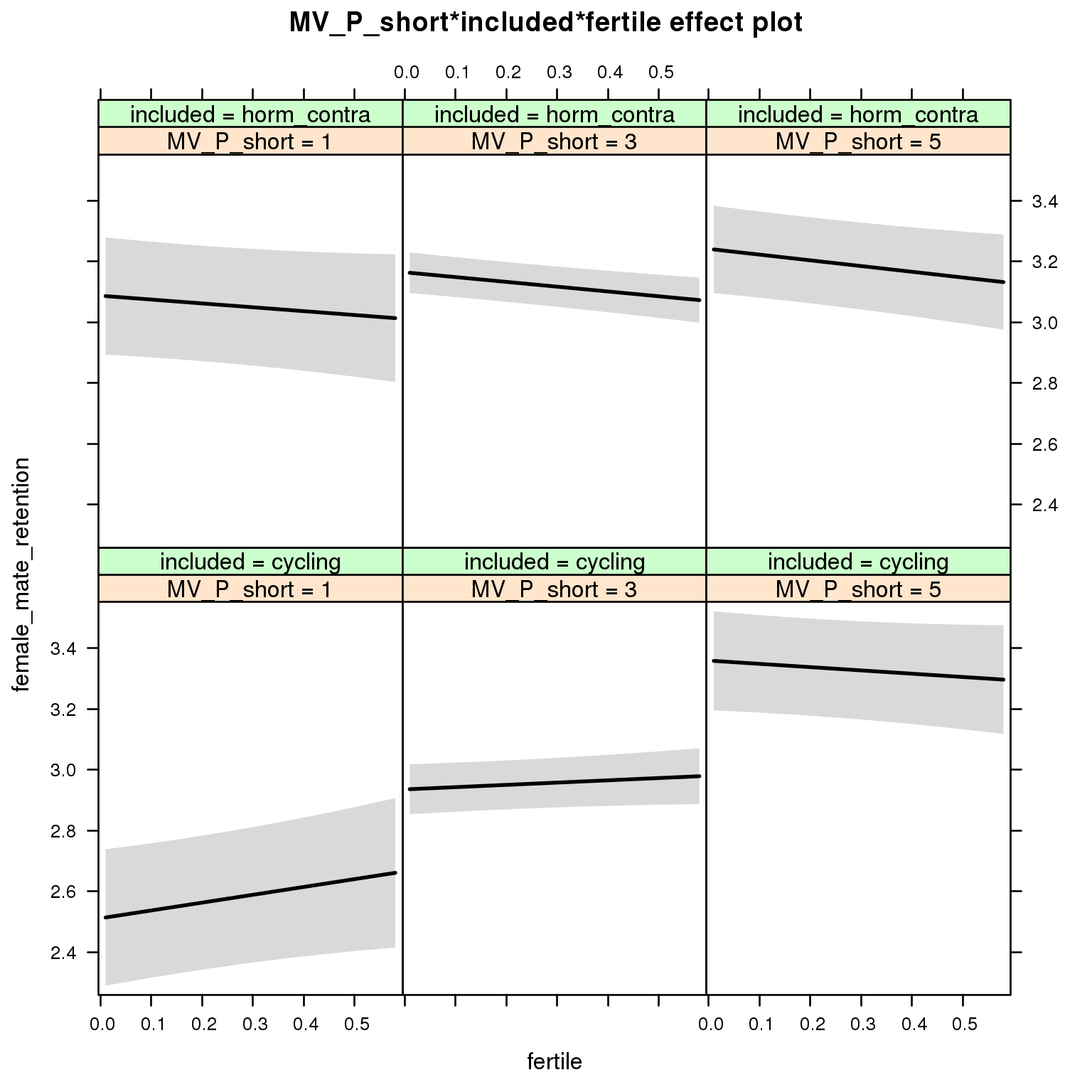
Linear mixed model fit by REML ['lmerMod']
Formula: female_mate_retention ~ menstruation + fertile_mean + (1 | person) +
MV_P_short + included + fertile + menstruation:included +
MV_P_short:included + MV_P_short:fertile + included:fertile + MV_P_short:included:fertile
Data: diary
REML criterion at convergence: 69601
Scaled residuals:
Min 1Q Median 3Q Max
-4.145 -0.628 -0.003 0.629 4.516
Random effects:
Groups Name Variance Std.Dev.
person (Intercept) 0.532 0.730
Residual 0.712 0.844
Number of obs: 26681, groups: person, 1054
Fixed effects:
Estimate Std. Error t value
(Intercept) 2.32322 0.16568 14.02
menstruationpre -0.00948 0.02576 -0.37
menstruationyes 0.01687 0.02428 0.69
fertile_mean -0.14728 0.28832 -0.51
MV_P_short 0.21219 0.04557 4.66
includedhorm_contra 0.75951 0.21006 3.62
fertile 0.34960 0.18816 1.86
menstruationpre:includedhorm_contra -0.03248 0.03307 -0.98
menstruationyes:includedhorm_contra -0.02231 0.03183 -0.70
MV_P_short:includedhorm_contra -0.17366 0.06064 -2.86
MV_P_short:fertile -0.09155 0.05381 -1.70
includedhorm_contra:fertile -0.46168 0.24309 -1.90
MV_P_short:includedhorm_contra:fertile 0.07627 0.06982 1.09
Partner’s job and income
model %>%
test_moderator("partner_attractiveness_money", diary)refitting model(s) with ML (instead of REML)
| Df | AIC | BIC | logLik | deviance | Chisq | Chi Df | Pr(>Chisq) | |
|---|---|---|---|---|---|---|---|---|
| with_main | 13 | 69589 | 69695 | -34781 | 69563 | NA | NA | NA |
| with_mod | 15 | 69593 | 69715 | -34781 | 69563 | 0.0559 | 2 | 0.9724 |
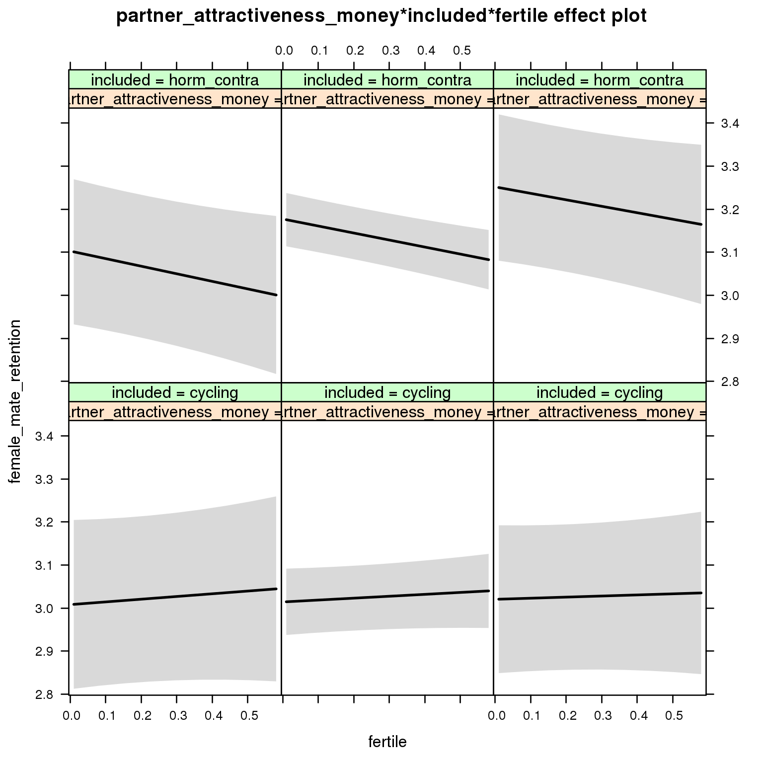
Linear mixed model fit by REML ['lmerMod']
Formula: female_mate_retention ~ menstruation + fertile_mean + (1 | person) +
partner_attractiveness_money + included + fertile + menstruation:included +
partner_attractiveness_money:included + partner_attractiveness_money:fertile +
included:fertile + partner_attractiveness_money:included:fertile
Data: diary
REML criterion at convergence: 69623
Scaled residuals:
Min 1Q Median 3Q Max
-4.152 -0.628 -0.004 0.632 4.539
Random effects:
Groups Name Variance Std.Dev.
person (Intercept) 0.543 0.737
Residual 0.712 0.844
Number of obs: 26681, groups: person, 1054
Fixed effects:
Estimate Std. Error t value
(Intercept) 3.02783 0.15024 20.15
menstruationpre -0.00849 0.02576 -0.33
menstruationyes 0.01774 0.02428 0.73
fertile_mean -0.13971 0.29076 -0.48
partner_attractiveness_money 0.00309 0.04279 0.07
includedhorm_contra 0.07052 0.18839 0.37
fertile 0.07243 0.16541 0.44
menstruationpre:includedhorm_contra -0.03347 0.03308 -1.01
menstruationyes:includedhorm_contra -0.02312 0.03183 -0.73
partner_attractiveness_money:includedhorm_contra 0.03417 0.05877 0.58
partner_attractiveness_money:fertile -0.00939 0.04950 -0.19
includedhorm_contra:fertile -0.25477 0.21709 -1.17
partner_attractiveness_money:includedhorm_contra:fertile 0.01584 0.06708 0.24
Sexy clothes
model_summaries$sexy_clothesModel summary
Model summary
model %>%
print_summary()Linear mixed model fit by REML
t-tests use Satterthwaite approximations to degrees of freedom ['lmerMod']
Formula: sexy_clothes ~ included * (menstruation + fertile) + fertile_mean + (1 | person)
Data: diary
REML criterion at convergence: 75851
Scaled residuals:
Min 1Q Median 3Q Max
-4.225 -0.609 -0.020 0.617 4.498
Random effects:
Groups Name Variance Std.Dev.
person (Intercept) 0.583 0.763
Residual 0.904 0.951
Number of obs: 26688, groups: person, 1054
Fixed effects:
Estimate Std. Error df t value Pr(>|t|)
(Intercept) 2.9647 0.0670 1416.0000 44.28 < 2e-16 ***
includedhorm_contra 0.1234 0.0548 1378.0000 2.25 0.0246 *
menstruationpre -0.0948 0.0290 26010.0000 -3.27 0.0011 **
menstruationyes -0.1432 0.0273 26119.0000 -5.24 0.00000016 ***
fertile -0.0388 0.0586 25993.0000 -0.66 0.5075
fertile_mean 0.6097 0.3073 1536.0000 1.98 0.0474 *
includedhorm_contra:menstruationpre 0.0358 0.0373 26007.0000 0.96 0.3370
includedhorm_contra:menstruationyes 0.0889 0.0358 26096.0000 2.48 0.0132 *
includedhorm_contra:fertile -0.0928 0.0742 26120.0000 -1.25 0.2111
---
Signif. codes: 0 '***' 0.001 '**' 0.01 '*' 0.05 '.' 0.1 ' ' 1
Correlation of Fixed Effects:
(Intr) incld_ mnstrtnp mnstrtny fertil frtl_m inclddhrm_cntr:mnstrtnp
inclddhrm_c -0.473
menstrutnpr -0.167 0.211
menstrutnys -0.163 0.204 0.397
fertile -0.160 0.262 0.467 0.384
fertile_men -0.772 -0.026 -0.008 -0.005 -0.068
inclddhrm_cntr:mnstrtnp 0.138 -0.265 -0.779 -0.309 -0.363 -0.004
inclddhrm_cntr:mnstrtny 0.130 -0.250 -0.303 -0.763 -0.293 -0.004 0.383
inclddhrm_cntr:f 0.160 -0.331 -0.368 -0.303 -0.786 0.010 0.466
inclddhrm_cntr:mnstrtny
inclddhrm_c
menstrutnpr
menstrutnys
fertile
fertile_men
inclddhrm_cntr:mnstrtnp
inclddhrm_cntr:mnstrtny
inclddhrm_cntr:f 0.381
Effect size standardised by residual variance (\(\frac{b}{ SD_{residual} }\)): -0.04 [-0.16;0.08].
Marginal effect plots
model %>%
plot_all_effects()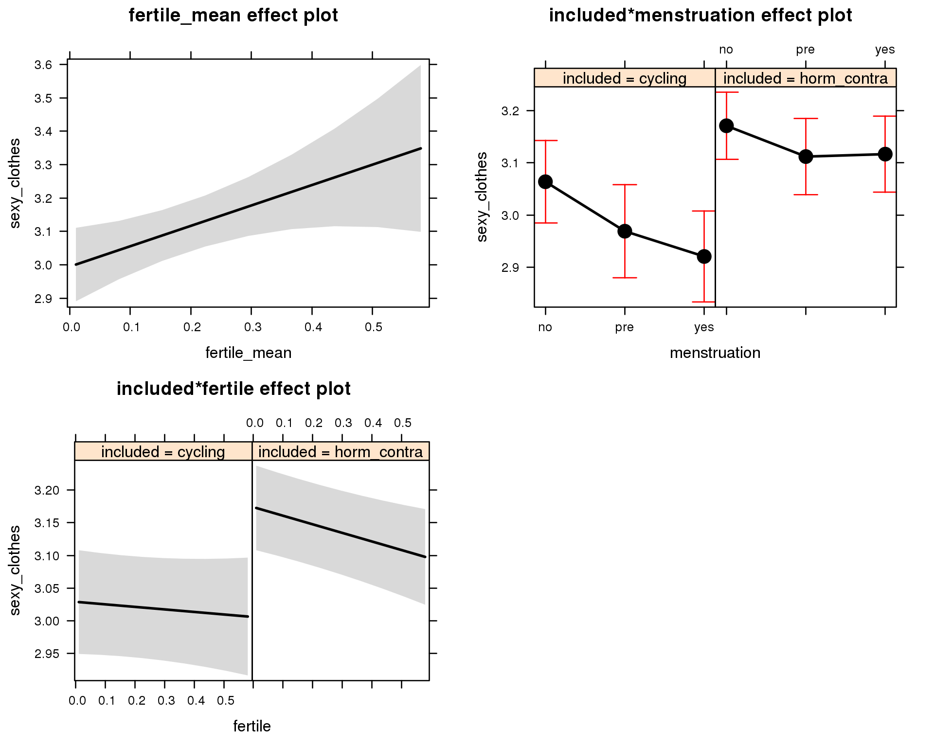
Outcome distribution
model %>%
plot_outcome(diary) + xlab(outcome_label)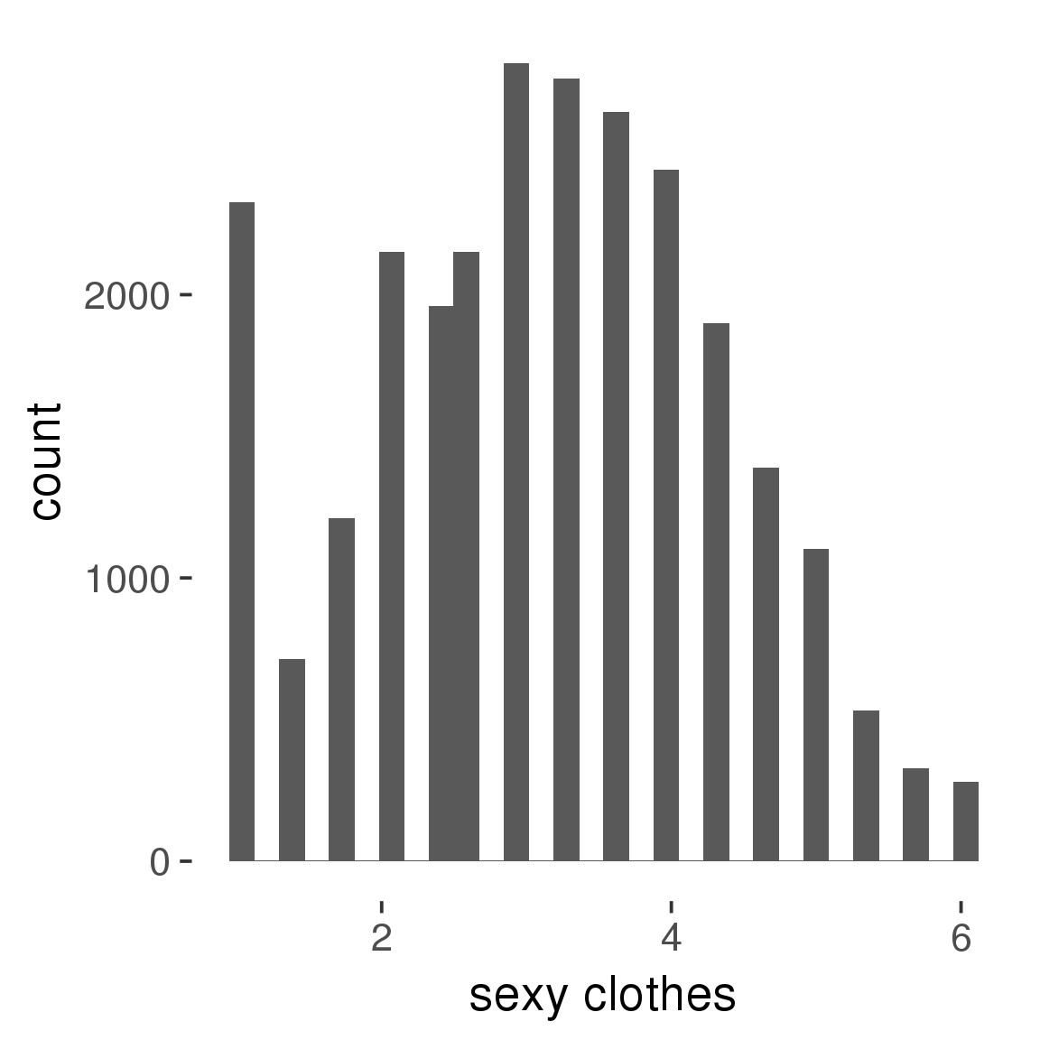
Diagnostics
model %>%
print_diagnostics()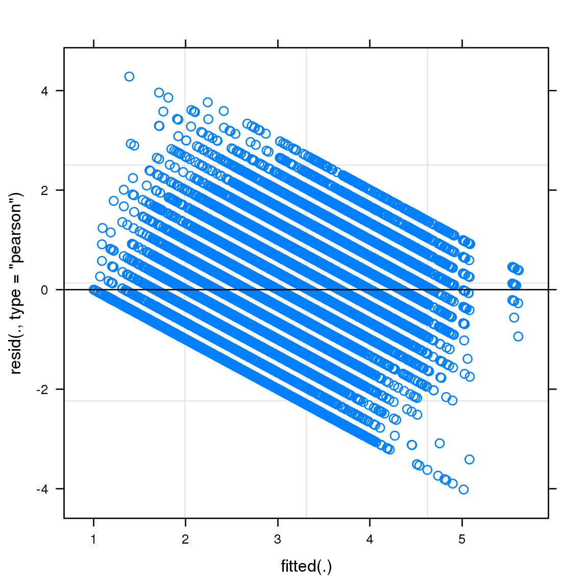
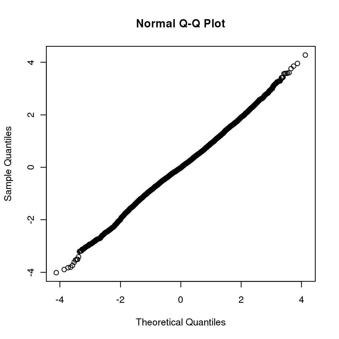

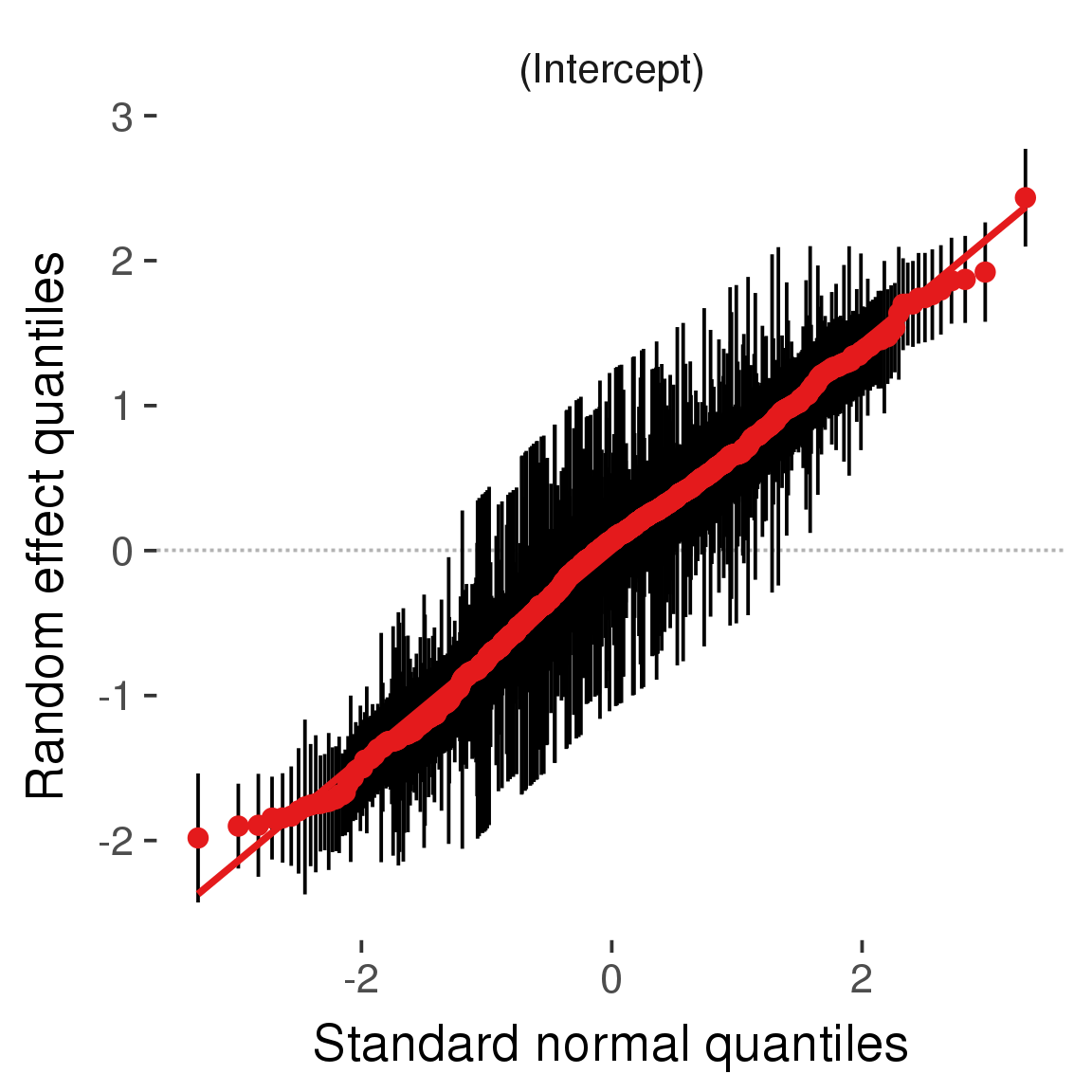
Curves
Here, we continuously plot the outcome over the course of the cycle. Because cycle lengths vary, we subset the data to cycles in a certain range. If the red curve traces the pink curve, our predictor accurately maps the relationship between fertile window probability and the outcome.
Cycle lengths from 21 to 36
Backward-counted
model %>%
plot_curve(diary %>% filter(minimum_cycle_length_diary <= 36, minimum_cycle_length_diary > 20) %>% mutate(fertile=prc_stirn_b))outcome = names(model@frame)[1]
outcome_label = recode(str_replace_all(str_replace_all(str_replace_all(outcome, "_", " "), " pair", "-pair"), " 1", ""),
"desirability 1" = "self-perceived desirability",
"NARQ admiration" = "narcissistic admiration",
"NARQ rivalry" = "narcissistic rivalry",
"extra-pair" = "extra-pair desire & behaviour",
"had sexual intercourse" = "sexual intercourse")
library(ggplot2)
# form a subset and run the model without the hormonal contraception and the fertility predictors
tmp = diary %>%
filter(!is.na(fertile), !is.na(included),
RCD > -1 * minimum_cycle_length_diary, RCD > -40)
new_form = update.formula(formula(model), new = . ~ . - fertile * included)
tmp$residuals = residuals(update(model, new_form, data = tmp , na.action = na.exclude))
tmp = tmp %>%
filter(!is.na(RCD), !is.na(residuals))
rcd_min = min(tmp$RCD)
tmp$real = FALSE
tmp_before = tmp
tmp_before$RCD = tmp_before$RCD + min(tmp$RCD) - 1
tmp_after = tmp
tmp_after$RCD = tmp_after$RCD - min(tmp$RCD) + 1
tmp$real = TRUE
tmp = bind_rows(tmp_before %>% filter(RCD > rcd_min - 11), tmp, tmp_after %>% filter(RCD < 11))GAM smooth on residuals
Here, we partialled out menstruation and individual random effects, then superimposed estimated probability of being in the fertile window scaled to the range of the estimated means. To address the periodicity of the cycle, we prepended and appended ten days of the timeseries to the end and the beginning of the timeseries. We then estimated the GAM and cut off the appended subsets before plotting.
tryCatch({
trend_plot = ggplot(tmp,aes(x = RCD, y = residuals, colour = included)) +
stat_smooth(geom = 'smooth',size = 0.8, fill = "#9ECAE1", method = 'gam', formula = y ~ s(x))
}, error = function(e){cat_message(e, "danger")})
tryCatch({
trend_data = ggplot_build(trend_plot)$data[[1]]
}, error = function(e){cat_message(e, "danger")})
trend_data$RCD = round(trend_data$x)
trend_data = left_join(trend_data, tmp %>% select(real, RCD,fertile) %>% unique(), by = "RCD")
trend_data %>%
filter(real == TRUE) %>%
mutate(superimposed = ( ( (fertile - 0.01)/0.58) * (max(y)-min(y) ) ) + min(y) ) ->
trend_data
ggplot(trend_data) +
geom_ribbon(aes(x = x, ymin = ymin, ymax = ymax, fill = factor(group)), alpha = 0.2) +
geom_line(aes(x = x, y = y, colour = factor(group)), size = 0.8, stat = "identity") +
scale_x_continuous(caption_x) +
geom_line(aes(x = x, y = superimposed), color = "#a83fbf", size = 1, linetype = 'dashed') +
annotate("text",x = mean(trend_data$x), y = max(trend_data$superimposed,na.rm=T) + 0.1, label = 'superimposed fertility peak', color = "#a83fbf") +
scale_y_continuous(outcome_label) +
ggtitle("GAM smooth, residuals") +
scale_color_manual("Contraception status",values = c("2"="black","1"= "red"), labels = c("2"="hormonally\ncontracepting","1"="cycling"), guide = F) +
scale_fill_manual("Contraception status",values = c("2"="black","1"= "red"), labels = c("2"="hormonally\ncontracepting","1"="cycling"), guide = F)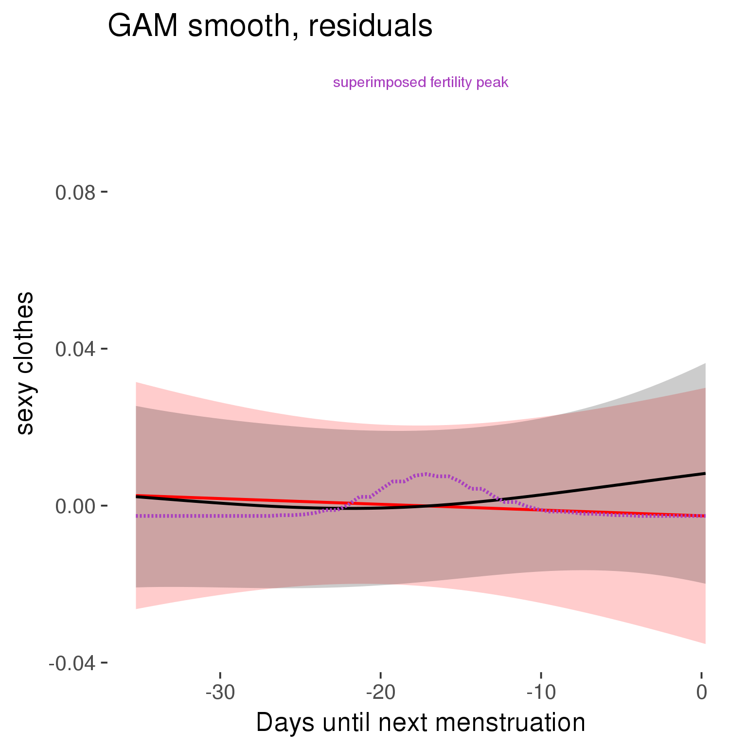
GAM smooth on raw data
As before, but without partialling anything out.
tryCatch({
trend_plot = ggplot(tmp,aes_string(x = "RCD", y = outcome, colour = "included")) +
stat_smooth(geom = 'smooth',size = 0.8, fill = "#9ECAE1", method = 'gam', formula = y ~ s(x))
}, error = function(e){cat_message(e, "danger")})
tryCatch({
trend_data = ggplot_build(trend_plot)$data[[1]]
}, error = function(e){cat_message(e, "danger")})
trend_data$RCD = round(trend_data$x)
trend_data = left_join(trend_data, tmp %>% select(real, RCD,fertile) %>% unique(), by = "RCD")
trend_data %>%
filter(real == TRUE) %>%
mutate(superimposed = ( ( (fertile - 0.01)/0.58) * (max(y)-min(y) ) ) + min(y) ) ->
trend_data
plot1b = ggplot(trend_data) +
geom_ribbon(aes(x = x, ymin = ymin, ymax = ymax, fill = factor(group)), alpha = 0.2) +
geom_line(aes(x = x, y = y, colour = factor(group)), size = 0.8, stat = "identity") +
scale_x_continuous(caption_x) +
geom_line(aes(x = x, y = superimposed), color = "#a83fbf", size = 1, linetype = 'dashed') +
annotate("text",x = mean(trend_data$x), y = max(trend_data$superimposed,na.rm=T) + 0.1, label = 'superimposed fertility peak', color = "#a83fbf") +
scale_y_continuous(outcome_label) +
ggtitle("GAM smooth, raw data") +
scale_color_manual("Contraception status",values = c("2"="black","1"= "red"), labels = c("2"="hormonally\ncontracepting","1"="cycling"), guide = F) +
scale_fill_manual("Contraception status",values = c("2"="black","1"= "red"), labels = c("2"="hormonally\ncontracepting","1"="cycling"), guide = F)
suppressWarnings(print(plot1b))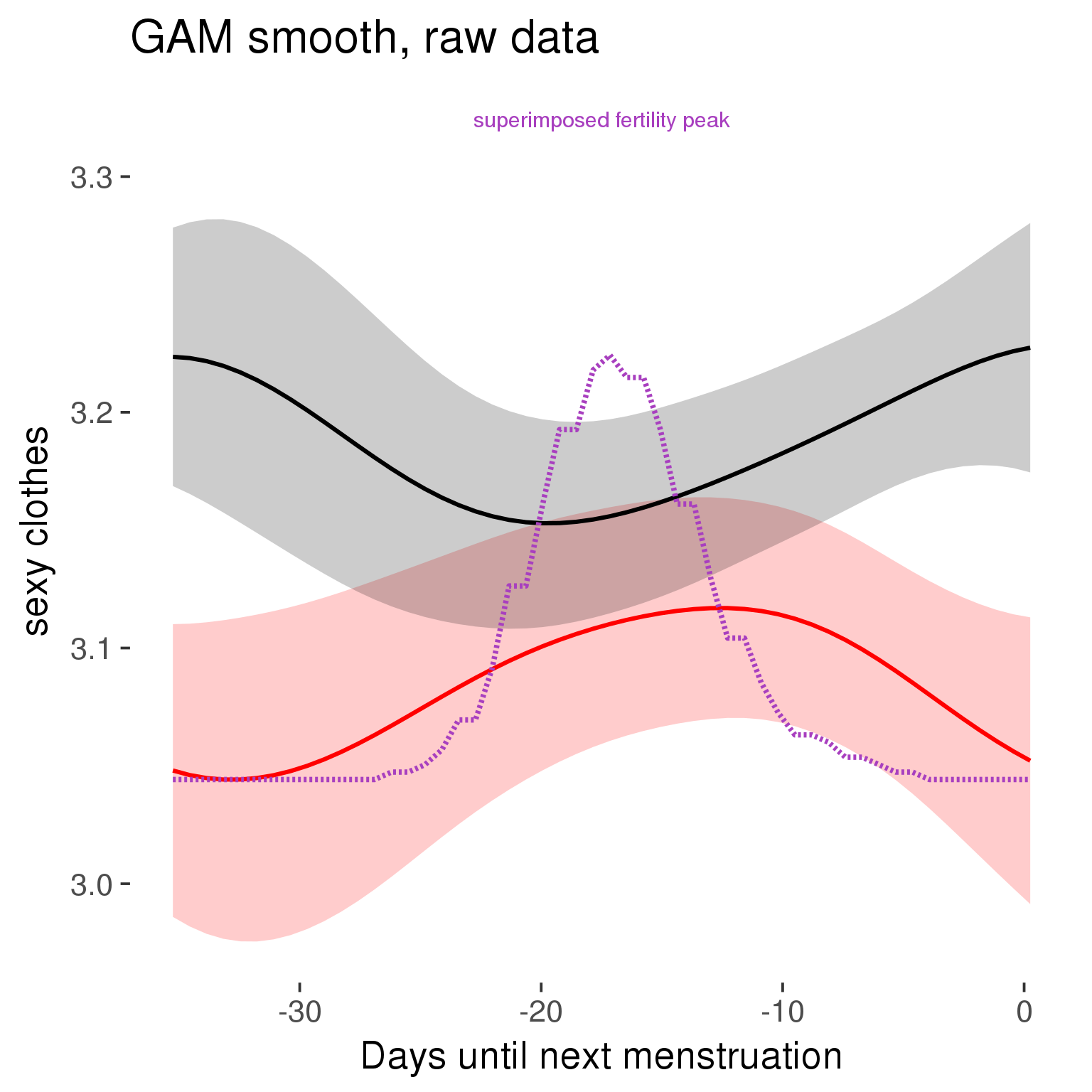
Means and standard errors over raw data
Nothing partialled out, just straight means with bootstrapped confidence intervals.
tryCatch({
trend_plot = ggplot(tmp,aes_string(x = "RCD", y = outcome, colour = "included")) +
geom_pointrange(size = 0.8, stat = 'summary', fun.data = "mean_cl_boot")
}, error = function(e){cat_message(e, "danger")})
tryCatch({
trend_data = ggplot_build(trend_plot)$data[[1]]
}, error = function(e){cat_message(e, "danger")})
trend_data$RCD = round(trend_data$x)
trend_data = left_join(trend_data, tmp %>% select(real, RCD,fertile) %>% unique(), by = "RCD")
trend_data %>%
filter(real == TRUE) %>%
mutate(superimposed = ( ( (fertile - 0.01)/0.58) * (max(y)-min(y) ) ) + min(y) ) ->
trend_data
plot3 = ggplot(trend_data) +
geom_pointrange(aes(x = x, y = y, ymin = ymin,ymax = ymax, colour = factor(group)), size = 0.8, stat = "identity", alpha = 0.6, position = position_dodge(width = .5)) +
scale_x_continuous("Days until next menstruation") +
geom_line(aes(x= x, y = superimposed), color = "#a83fbf", size = 1, linetype = 'dashed') +
annotate("text",x = mean(trend_data$x), y = max(trend_data$superimposed,na.rm=T) + 0.1, label = 'superimposed fertility peak', color = "#a83fbf") +
scale_y_continuous(outcome_label) +
ggtitle("Means with standard errors, raw data") +
scale_color_manual("Contraception status",values = c("2"="black","1"= "red"), labels = c("2"="hormonally\ncontracepting","1"="cycling"), guide = F) +
scale_fill_manual("Contraception status",values = c("2"="black","1"= "red"), labels = c("2"="hormonally\ncontracepting","1"="cycling"), guide = F)
suppressWarnings(print(plot3))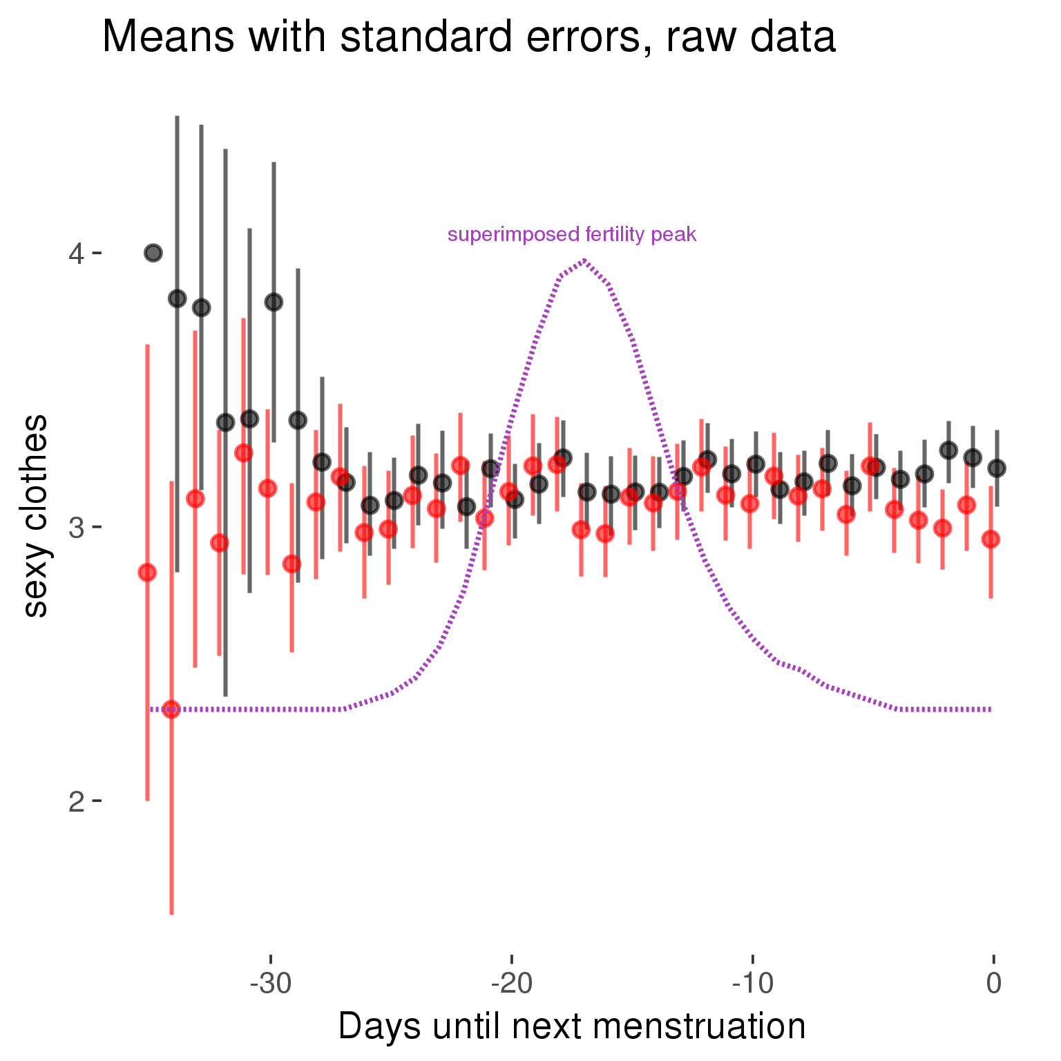
Forward-counted
model %>%
plot_curve(diary %>% filter(minimum_cycle_length_diary <= 36, minimum_cycle_length_diary > 20) %>% mutate(RCD = FCD, fertile = prc_stirn_b_forward_counted), caption_x = "Days since last menstruation")outcome = names(model@frame)[1]
outcome_label = recode(str_replace_all(str_replace_all(str_replace_all(outcome, "_", " "), " pair", "-pair"), " 1", ""),
"desirability 1" = "self-perceived desirability",
"NARQ admiration" = "narcissistic admiration",
"NARQ rivalry" = "narcissistic rivalry",
"extra-pair" = "extra-pair desire & behaviour",
"had sexual intercourse" = "sexual intercourse")
library(ggplot2)
# form a subset and run the model without the hormonal contraception and the fertility predictors
tmp = diary %>%
filter(!is.na(fertile), !is.na(included),
RCD > -1 * minimum_cycle_length_diary, RCD > -40)
new_form = update.formula(formula(model), new = . ~ . - fertile * included)
tmp$residuals = residuals(update(model, new_form, data = tmp , na.action = na.exclude))
tmp = tmp %>%
filter(!is.na(RCD), !is.na(residuals))
rcd_min = min(tmp$RCD)
tmp$real = FALSE
tmp_before = tmp
tmp_before$RCD = tmp_before$RCD + min(tmp$RCD) - 1
tmp_after = tmp
tmp_after$RCD = tmp_after$RCD - min(tmp$RCD) + 1
tmp$real = TRUE
tmp = bind_rows(tmp_before %>% filter(RCD > rcd_min - 11), tmp, tmp_after %>% filter(RCD < 11))GAM smooth on residuals
Here, we partialled out menstruation and individual random effects, then superimposed estimated probability of being in the fertile window scaled to the range of the estimated means. To address the periodicity of the cycle, we prepended and appended ten days of the timeseries to the end and the beginning of the timeseries. We then estimated the GAM and cut off the appended subsets before plotting.
tryCatch({
trend_plot = ggplot(tmp,aes(x = RCD, y = residuals, colour = included)) +
stat_smooth(geom = 'smooth',size = 0.8, fill = "#9ECAE1", method = 'gam', formula = y ~ s(x))
}, error = function(e){cat_message(e, "danger")})
tryCatch({
trend_data = ggplot_build(trend_plot)$data[[1]]
}, error = function(e){cat_message(e, "danger")})
trend_data$RCD = round(trend_data$x)
trend_data = left_join(trend_data, tmp %>% select(real, RCD,fertile) %>% unique(), by = "RCD")
trend_data %>%
filter(real == TRUE) %>%
mutate(superimposed = ( ( (fertile - 0.01)/0.58) * (max(y)-min(y) ) ) + min(y) ) ->
trend_data
ggplot(trend_data) +
geom_ribbon(aes(x = x, ymin = ymin, ymax = ymax, fill = factor(group)), alpha = 0.2) +
geom_line(aes(x = x, y = y, colour = factor(group)), size = 0.8, stat = "identity") +
scale_x_continuous(caption_x) +
geom_line(aes(x = x, y = superimposed), color = "#a83fbf", size = 1, linetype = 'dashed') +
annotate("text",x = mean(trend_data$x), y = max(trend_data$superimposed,na.rm=T) + 0.1, label = 'superimposed fertility peak', color = "#a83fbf") +
scale_y_continuous(outcome_label) +
ggtitle("GAM smooth, residuals") +
scale_color_manual("Contraception status",values = c("2"="black","1"= "red"), labels = c("2"="hormonally\ncontracepting","1"="cycling"), guide = F) +
scale_fill_manual("Contraception status",values = c("2"="black","1"= "red"), labels = c("2"="hormonally\ncontracepting","1"="cycling"), guide = F)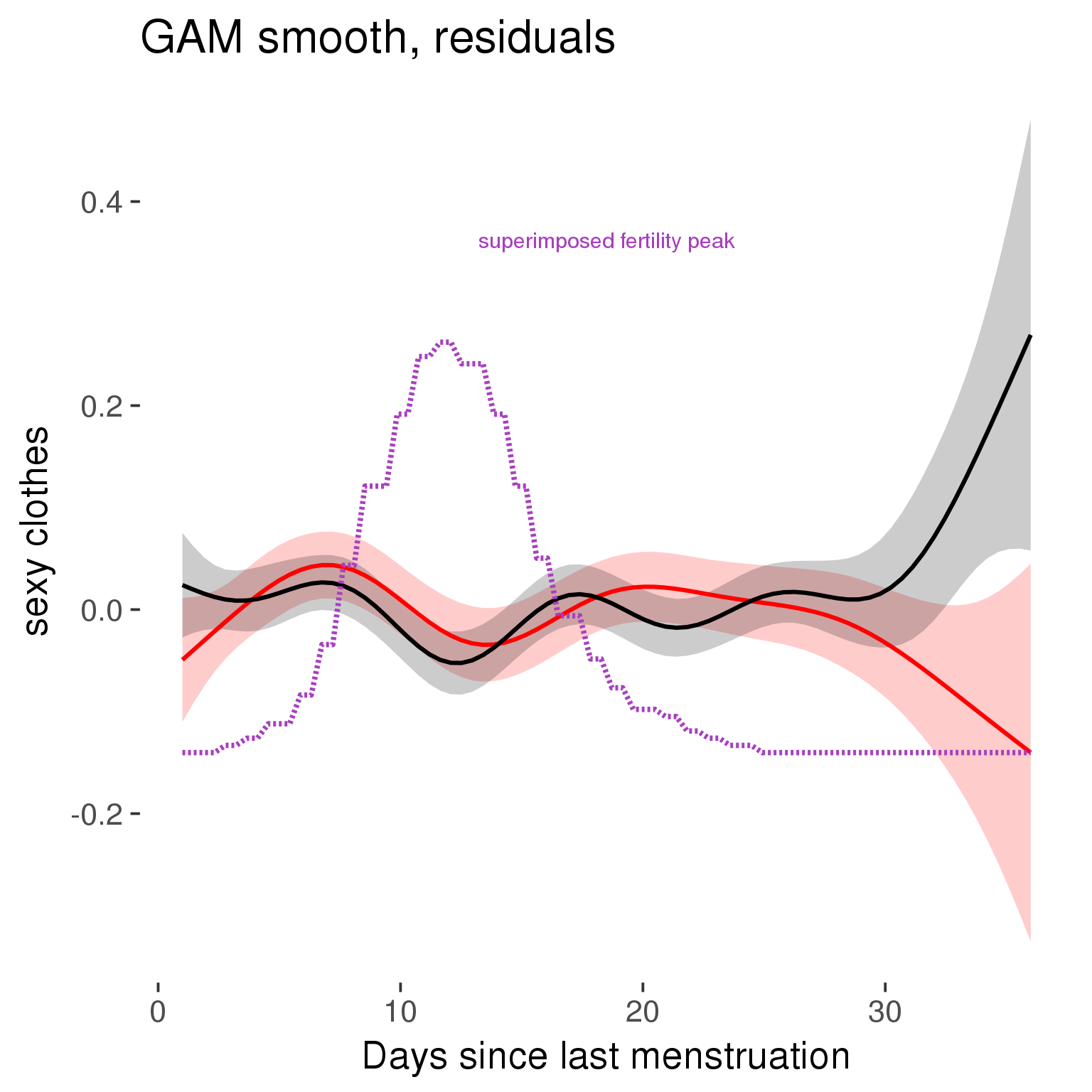
GAM smooth on raw data
As before, but without partialling anything out.
tryCatch({
trend_plot = ggplot(tmp,aes_string(x = "RCD", y = outcome, colour = "included")) +
stat_smooth(geom = 'smooth',size = 0.8, fill = "#9ECAE1", method = 'gam', formula = y ~ s(x))
}, error = function(e){cat_message(e, "danger")})
tryCatch({
trend_data = ggplot_build(trend_plot)$data[[1]]
}, error = function(e){cat_message(e, "danger")})
trend_data$RCD = round(trend_data$x)
trend_data = left_join(trend_data, tmp %>% select(real, RCD,fertile) %>% unique(), by = "RCD")
trend_data %>%
filter(real == TRUE) %>%
mutate(superimposed = ( ( (fertile - 0.01)/0.58) * (max(y)-min(y) ) ) + min(y) ) ->
trend_data
plot1b = ggplot(trend_data) +
geom_ribbon(aes(x = x, ymin = ymin, ymax = ymax, fill = factor(group)), alpha = 0.2) +
geom_line(aes(x = x, y = y, colour = factor(group)), size = 0.8, stat = "identity") +
scale_x_continuous(caption_x) +
geom_line(aes(x = x, y = superimposed), color = "#a83fbf", size = 1, linetype = 'dashed') +
annotate("text",x = mean(trend_data$x), y = max(trend_data$superimposed,na.rm=T) + 0.1, label = 'superimposed fertility peak', color = "#a83fbf") +
scale_y_continuous(outcome_label) +
ggtitle("GAM smooth, raw data") +
scale_color_manual("Contraception status",values = c("2"="black","1"= "red"), labels = c("2"="hormonally\ncontracepting","1"="cycling"), guide = F) +
scale_fill_manual("Contraception status",values = c("2"="black","1"= "red"), labels = c("2"="hormonally\ncontracepting","1"="cycling"), guide = F)
suppressWarnings(print(plot1b))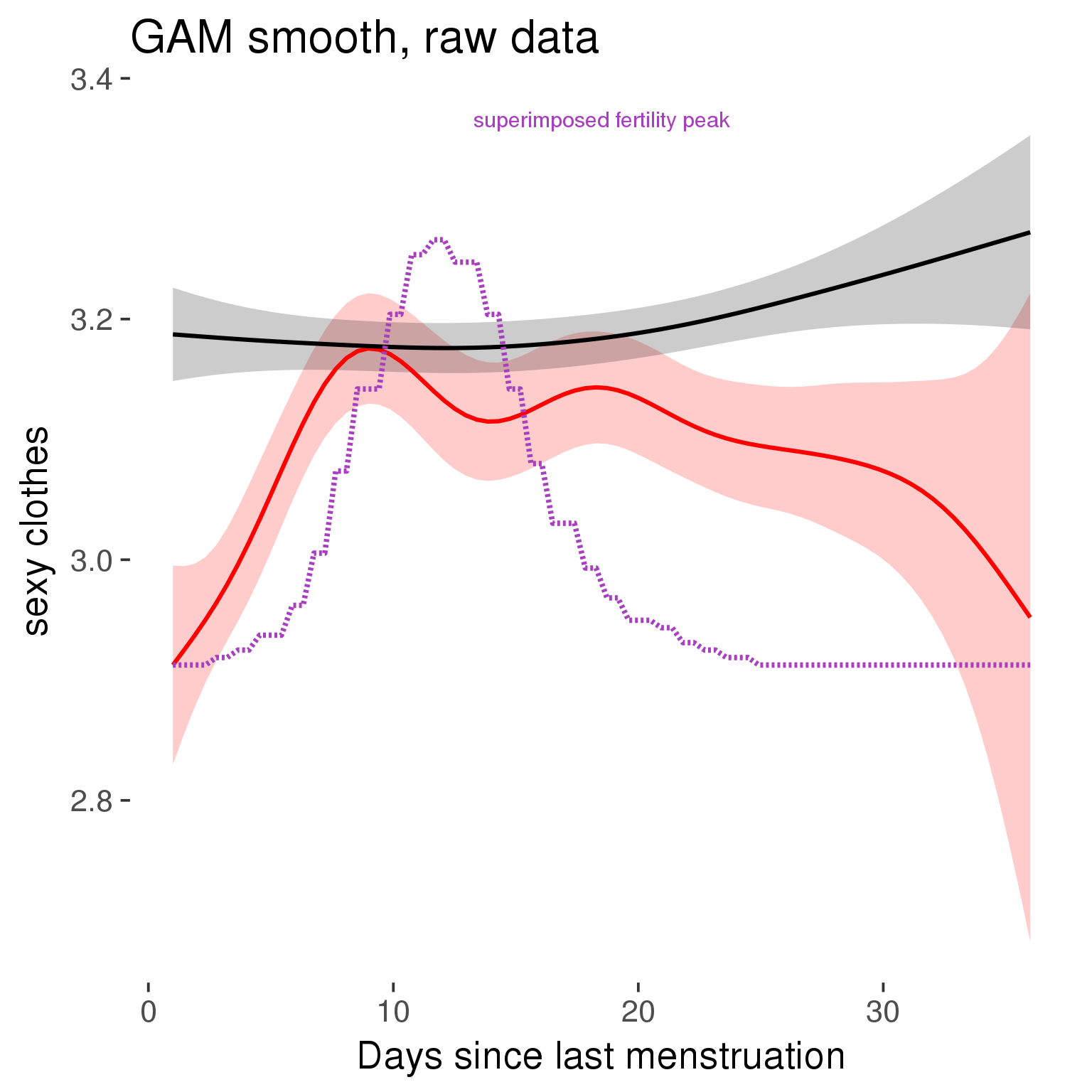
Means and standard errors over raw data
Nothing partialled out, just straight means with bootstrapped confidence intervals.
tryCatch({
trend_plot = ggplot(tmp,aes_string(x = "RCD", y = outcome, colour = "included")) +
geom_pointrange(size = 0.8, stat = 'summary', fun.data = "mean_cl_boot")
}, error = function(e){cat_message(e, "danger")})
tryCatch({
trend_data = ggplot_build(trend_plot)$data[[1]]
}, error = function(e){cat_message(e, "danger")})
trend_data$RCD = round(trend_data$x)
trend_data = left_join(trend_data, tmp %>% select(real, RCD,fertile) %>% unique(), by = "RCD")
trend_data %>%
filter(real == TRUE) %>%
mutate(superimposed = ( ( (fertile - 0.01)/0.58) * (max(y)-min(y) ) ) + min(y) ) ->
trend_data
plot3 = ggplot(trend_data) +
geom_pointrange(aes(x = x, y = y, ymin = ymin,ymax = ymax, colour = factor(group)), size = 0.8, stat = "identity", alpha = 0.6, position = position_dodge(width = .5)) +
scale_x_continuous("Days until next menstruation") +
geom_line(aes(x= x, y = superimposed), color = "#a83fbf", size = 1, linetype = 'dashed') +
annotate("text",x = mean(trend_data$x), y = max(trend_data$superimposed,na.rm=T) + 0.1, label = 'superimposed fertility peak', color = "#a83fbf") +
scale_y_continuous(outcome_label) +
ggtitle("Means with standard errors, raw data") +
scale_color_manual("Contraception status",values = c("2"="black","1"= "red"), labels = c("2"="hormonally\ncontracepting","1"="cycling"), guide = F) +
scale_fill_manual("Contraception status",values = c("2"="black","1"= "red"), labels = c("2"="hormonally\ncontracepting","1"="cycling"), guide = F)
suppressWarnings(print(plot3))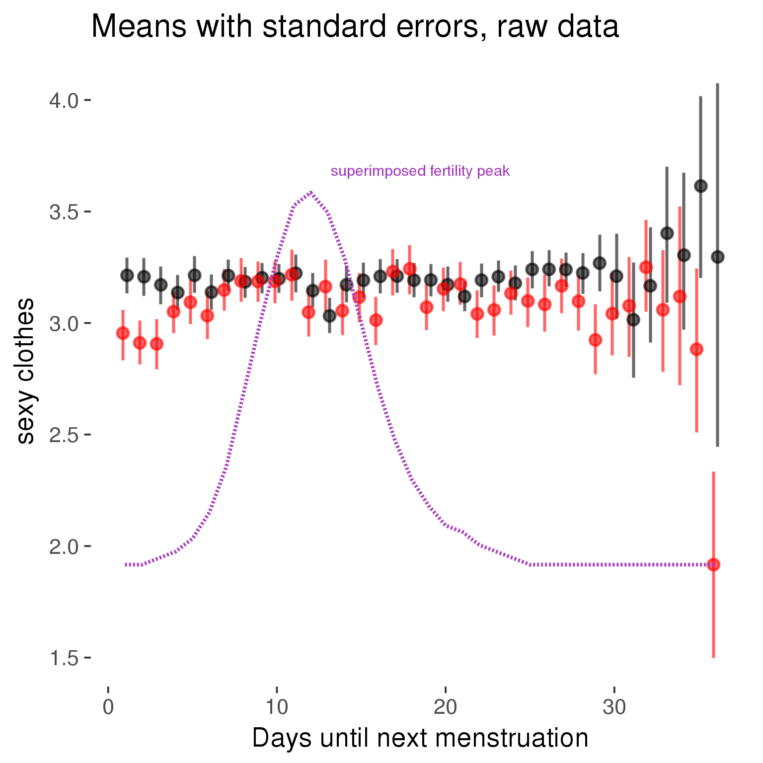
Cycle lengths from 27 to 30
Backward-counted
model %>%
plot_curve(diary %>% filter(minimum_cycle_length_diary <= 30, minimum_cycle_length_diary >= 27) %>% mutate(fertile=prc_stirn_b))outcome = names(model@frame)[1]
outcome_label = recode(str_replace_all(str_replace_all(str_replace_all(outcome, "_", " "), " pair", "-pair"), " 1", ""),
"desirability 1" = "self-perceived desirability",
"NARQ admiration" = "narcissistic admiration",
"NARQ rivalry" = "narcissistic rivalry",
"extra-pair" = "extra-pair desire & behaviour",
"had sexual intercourse" = "sexual intercourse")
library(ggplot2)
# form a subset and run the model without the hormonal contraception and the fertility predictors
tmp = diary %>%
filter(!is.na(fertile), !is.na(included),
RCD > -1 * minimum_cycle_length_diary, RCD > -40)
new_form = update.formula(formula(model), new = . ~ . - fertile * included)
tmp$residuals = residuals(update(model, new_form, data = tmp , na.action = na.exclude))
tmp = tmp %>%
filter(!is.na(RCD), !is.na(residuals))
rcd_min = min(tmp$RCD)
tmp$real = FALSE
tmp_before = tmp
tmp_before$RCD = tmp_before$RCD + min(tmp$RCD) - 1
tmp_after = tmp
tmp_after$RCD = tmp_after$RCD - min(tmp$RCD) + 1
tmp$real = TRUE
tmp = bind_rows(tmp_before %>% filter(RCD > rcd_min - 11), tmp, tmp_after %>% filter(RCD < 11))GAM smooth on residuals
Here, we partialled out menstruation and individual random effects, then superimposed estimated probability of being in the fertile window scaled to the range of the estimated means. To address the periodicity of the cycle, we prepended and appended ten days of the timeseries to the end and the beginning of the timeseries. We then estimated the GAM and cut off the appended subsets before plotting.
tryCatch({
trend_plot = ggplot(tmp,aes(x = RCD, y = residuals, colour = included)) +
stat_smooth(geom = 'smooth',size = 0.8, fill = "#9ECAE1", method = 'gam', formula = y ~ s(x))
}, error = function(e){cat_message(e, "danger")})
tryCatch({
trend_data = ggplot_build(trend_plot)$data[[1]]
}, error = function(e){cat_message(e, "danger")})
trend_data$RCD = round(trend_data$x)
trend_data = left_join(trend_data, tmp %>% select(real, RCD,fertile) %>% unique(), by = "RCD")
trend_data %>%
filter(real == TRUE) %>%
mutate(superimposed = ( ( (fertile - 0.01)/0.58) * (max(y)-min(y) ) ) + min(y) ) ->
trend_data
ggplot(trend_data) +
geom_ribbon(aes(x = x, ymin = ymin, ymax = ymax, fill = factor(group)), alpha = 0.2) +
geom_line(aes(x = x, y = y, colour = factor(group)), size = 0.8, stat = "identity") +
scale_x_continuous(caption_x) +
geom_line(aes(x = x, y = superimposed), color = "#a83fbf", size = 1, linetype = 'dashed') +
annotate("text",x = mean(trend_data$x), y = max(trend_data$superimposed,na.rm=T) + 0.1, label = 'superimposed fertility peak', color = "#a83fbf") +
scale_y_continuous(outcome_label) +
ggtitle("GAM smooth, residuals") +
scale_color_manual("Contraception status",values = c("2"="black","1"= "red"), labels = c("2"="hormonally\ncontracepting","1"="cycling"), guide = F) +
scale_fill_manual("Contraception status",values = c("2"="black","1"= "red"), labels = c("2"="hormonally\ncontracepting","1"="cycling"), guide = F)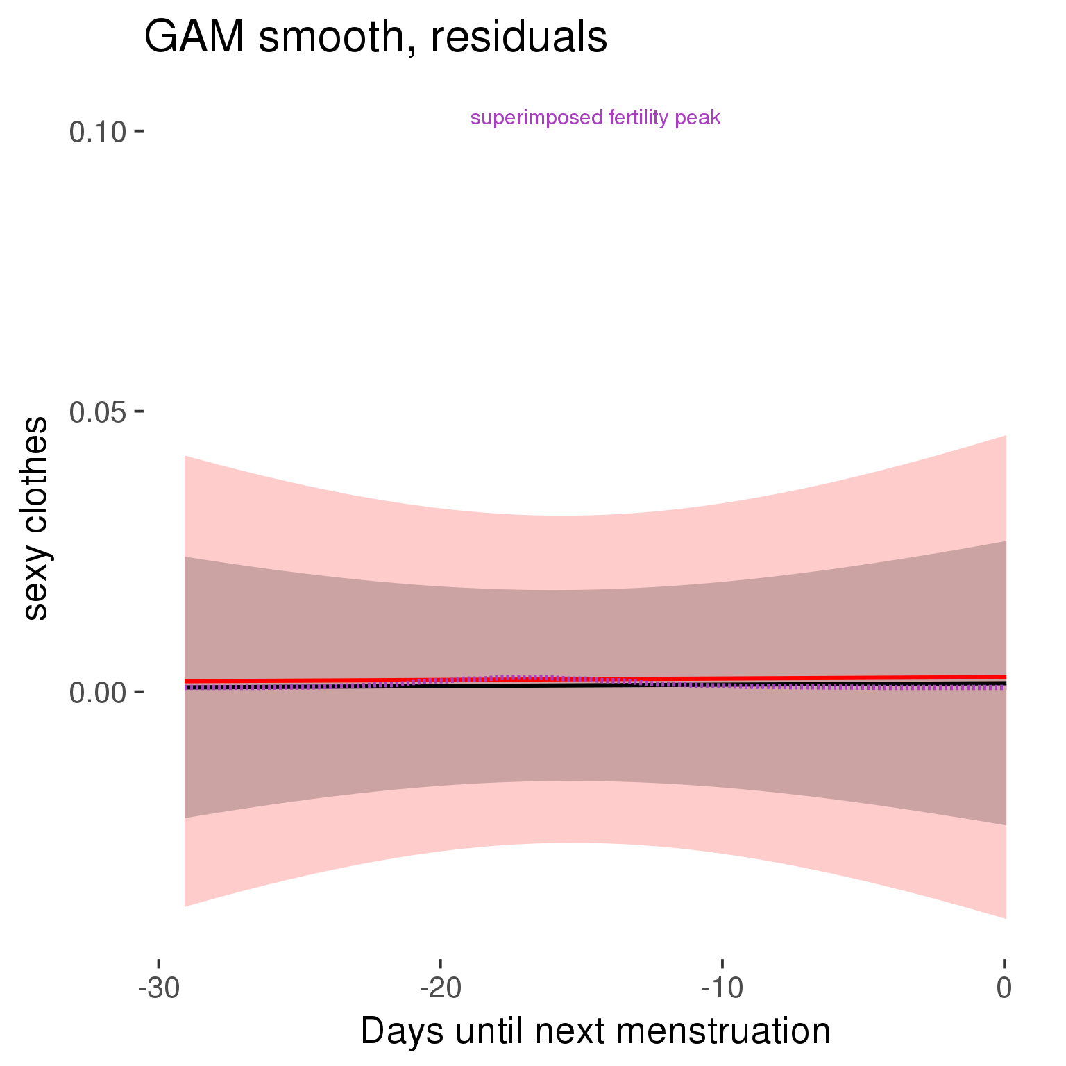
GAM smooth on raw data
As before, but without partialling anything out.
tryCatch({
trend_plot = ggplot(tmp,aes_string(x = "RCD", y = outcome, colour = "included")) +
stat_smooth(geom = 'smooth',size = 0.8, fill = "#9ECAE1", method = 'gam', formula = y ~ s(x))
}, error = function(e){cat_message(e, "danger")})
tryCatch({
trend_data = ggplot_build(trend_plot)$data[[1]]
}, error = function(e){cat_message(e, "danger")})
trend_data$RCD = round(trend_data$x)
trend_data = left_join(trend_data, tmp %>% select(real, RCD,fertile) %>% unique(), by = "RCD")
trend_data %>%
filter(real == TRUE) %>%
mutate(superimposed = ( ( (fertile - 0.01)/0.58) * (max(y)-min(y) ) ) + min(y) ) ->
trend_data
plot1b = ggplot(trend_data) +
geom_ribbon(aes(x = x, ymin = ymin, ymax = ymax, fill = factor(group)), alpha = 0.2) +
geom_line(aes(x = x, y = y, colour = factor(group)), size = 0.8, stat = "identity") +
scale_x_continuous(caption_x) +
geom_line(aes(x = x, y = superimposed), color = "#a83fbf", size = 1, linetype = 'dashed') +
annotate("text",x = mean(trend_data$x), y = max(trend_data$superimposed,na.rm=T) + 0.1, label = 'superimposed fertility peak', color = "#a83fbf") +
scale_y_continuous(outcome_label) +
ggtitle("GAM smooth, raw data") +
scale_color_manual("Contraception status",values = c("2"="black","1"= "red"), labels = c("2"="hormonally\ncontracepting","1"="cycling"), guide = F) +
scale_fill_manual("Contraception status",values = c("2"="black","1"= "red"), labels = c("2"="hormonally\ncontracepting","1"="cycling"), guide = F)
suppressWarnings(print(plot1b))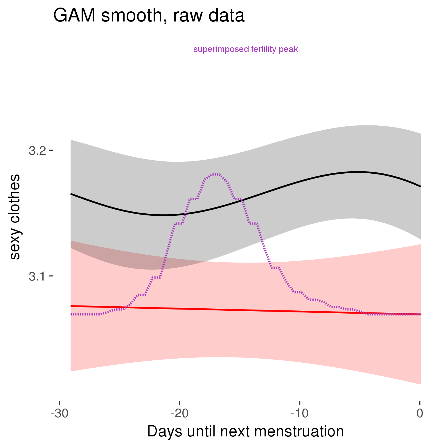
Means and standard errors over raw data
Nothing partialled out, just straight means with bootstrapped confidence intervals.
tryCatch({
trend_plot = ggplot(tmp,aes_string(x = "RCD", y = outcome, colour = "included")) +
geom_pointrange(size = 0.8, stat = 'summary', fun.data = "mean_cl_boot")
}, error = function(e){cat_message(e, "danger")})
tryCatch({
trend_data = ggplot_build(trend_plot)$data[[1]]
}, error = function(e){cat_message(e, "danger")})
trend_data$RCD = round(trend_data$x)
trend_data = left_join(trend_data, tmp %>% select(real, RCD,fertile) %>% unique(), by = "RCD")
trend_data %>%
filter(real == TRUE) %>%
mutate(superimposed = ( ( (fertile - 0.01)/0.58) * (max(y)-min(y) ) ) + min(y) ) ->
trend_data
plot3 = ggplot(trend_data) +
geom_pointrange(aes(x = x, y = y, ymin = ymin,ymax = ymax, colour = factor(group)), size = 0.8, stat = "identity", alpha = 0.6, position = position_dodge(width = .5)) +
scale_x_continuous("Days until next menstruation") +
geom_line(aes(x= x, y = superimposed), color = "#a83fbf", size = 1, linetype = 'dashed') +
annotate("text",x = mean(trend_data$x), y = max(trend_data$superimposed,na.rm=T) + 0.1, label = 'superimposed fertility peak', color = "#a83fbf") +
scale_y_continuous(outcome_label) +
ggtitle("Means with standard errors, raw data") +
scale_color_manual("Contraception status",values = c("2"="black","1"= "red"), labels = c("2"="hormonally\ncontracepting","1"="cycling"), guide = F) +
scale_fill_manual("Contraception status",values = c("2"="black","1"= "red"), labels = c("2"="hormonally\ncontracepting","1"="cycling"), guide = F)
suppressWarnings(print(plot3))
Forward-counted
model %>%
plot_curve(diary %>% filter(minimum_cycle_length_diary <= 30, minimum_cycle_length_diary >= 27) %>% mutate(RCD = FCD, fertile = prc_stirn_b_forward_counted), caption_x = "Days since last menstruation")outcome = names(model@frame)[1]
outcome_label = recode(str_replace_all(str_replace_all(str_replace_all(outcome, "_", " "), " pair", "-pair"), " 1", ""),
"desirability 1" = "self-perceived desirability",
"NARQ admiration" = "narcissistic admiration",
"NARQ rivalry" = "narcissistic rivalry",
"extra-pair" = "extra-pair desire & behaviour",
"had sexual intercourse" = "sexual intercourse")
library(ggplot2)
# form a subset and run the model without the hormonal contraception and the fertility predictors
tmp = diary %>%
filter(!is.na(fertile), !is.na(included),
RCD > -1 * minimum_cycle_length_diary, RCD > -40)
new_form = update.formula(formula(model), new = . ~ . - fertile * included)
tmp$residuals = residuals(update(model, new_form, data = tmp , na.action = na.exclude))
tmp = tmp %>%
filter(!is.na(RCD), !is.na(residuals))
rcd_min = min(tmp$RCD)
tmp$real = FALSE
tmp_before = tmp
tmp_before$RCD = tmp_before$RCD + min(tmp$RCD) - 1
tmp_after = tmp
tmp_after$RCD = tmp_after$RCD - min(tmp$RCD) + 1
tmp$real = TRUE
tmp = bind_rows(tmp_before %>% filter(RCD > rcd_min - 11), tmp, tmp_after %>% filter(RCD < 11))GAM smooth on residuals
Here, we partialled out menstruation and individual random effects, then superimposed estimated probability of being in the fertile window scaled to the range of the estimated means. To address the periodicity of the cycle, we prepended and appended ten days of the timeseries to the end and the beginning of the timeseries. We then estimated the GAM and cut off the appended subsets before plotting.
tryCatch({
trend_plot = ggplot(tmp,aes(x = RCD, y = residuals, colour = included)) +
stat_smooth(geom = 'smooth',size = 0.8, fill = "#9ECAE1", method = 'gam', formula = y ~ s(x))
}, error = function(e){cat_message(e, "danger")})
tryCatch({
trend_data = ggplot_build(trend_plot)$data[[1]]
}, error = function(e){cat_message(e, "danger")})
trend_data$RCD = round(trend_data$x)
trend_data = left_join(trend_data, tmp %>% select(real, RCD,fertile) %>% unique(), by = "RCD")
trend_data %>%
filter(real == TRUE) %>%
mutate(superimposed = ( ( (fertile - 0.01)/0.58) * (max(y)-min(y) ) ) + min(y) ) ->
trend_data
ggplot(trend_data) +
geom_ribbon(aes(x = x, ymin = ymin, ymax = ymax, fill = factor(group)), alpha = 0.2) +
geom_line(aes(x = x, y = y, colour = factor(group)), size = 0.8, stat = "identity") +
scale_x_continuous(caption_x) +
geom_line(aes(x = x, y = superimposed), color = "#a83fbf", size = 1, linetype = 'dashed') +
annotate("text",x = mean(trend_data$x), y = max(trend_data$superimposed,na.rm=T) + 0.1, label = 'superimposed fertility peak', color = "#a83fbf") +
scale_y_continuous(outcome_label) +
ggtitle("GAM smooth, residuals") +
scale_color_manual("Contraception status",values = c("2"="black","1"= "red"), labels = c("2"="hormonally\ncontracepting","1"="cycling"), guide = F) +
scale_fill_manual("Contraception status",values = c("2"="black","1"= "red"), labels = c("2"="hormonally\ncontracepting","1"="cycling"), guide = F)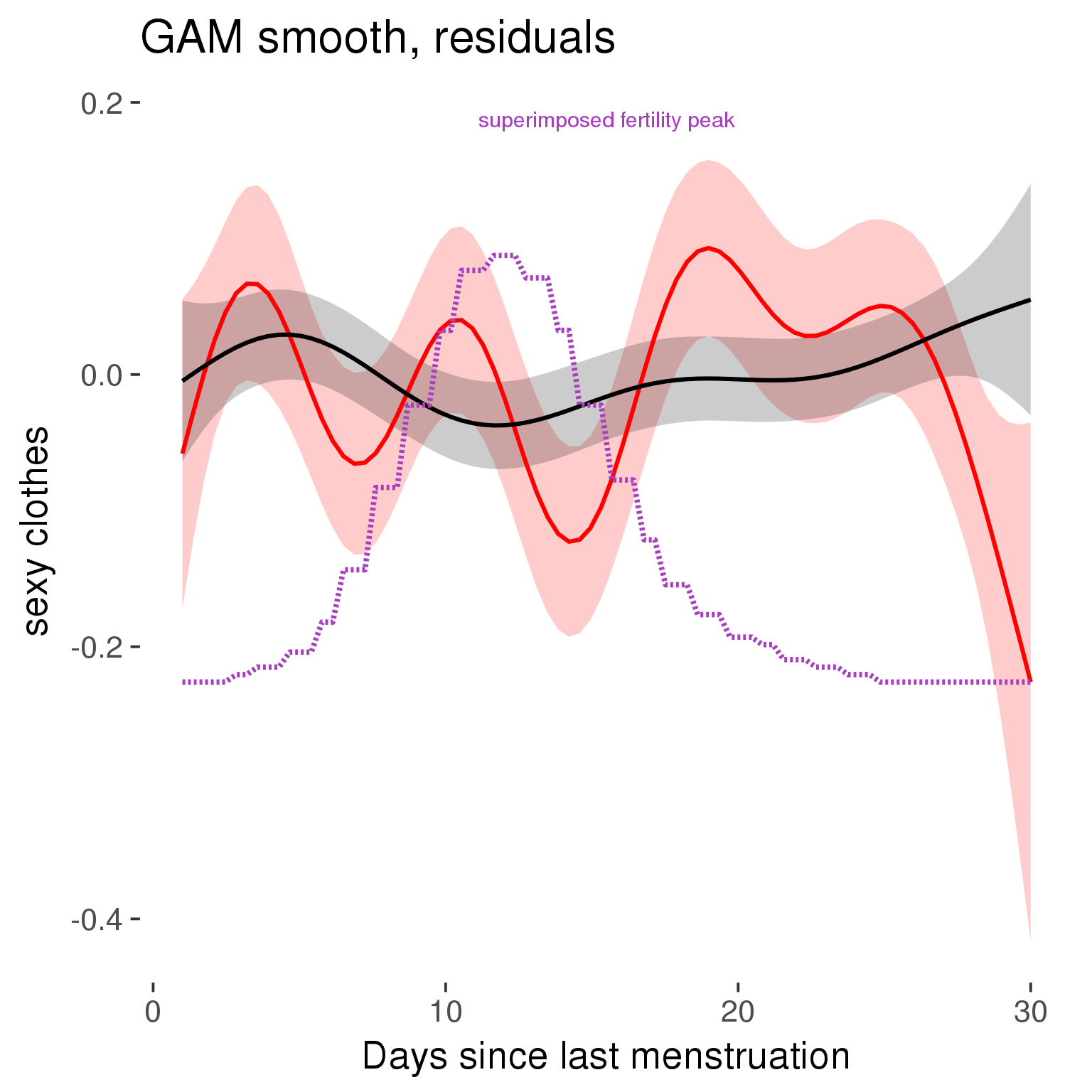
GAM smooth on raw data
As before, but without partialling anything out.
tryCatch({
trend_plot = ggplot(tmp,aes_string(x = "RCD", y = outcome, colour = "included")) +
stat_smooth(geom = 'smooth',size = 0.8, fill = "#9ECAE1", method = 'gam', formula = y ~ s(x))
}, error = function(e){cat_message(e, "danger")})
tryCatch({
trend_data = ggplot_build(trend_plot)$data[[1]]
}, error = function(e){cat_message(e, "danger")})
trend_data$RCD = round(trend_data$x)
trend_data = left_join(trend_data, tmp %>% select(real, RCD,fertile) %>% unique(), by = "RCD")
trend_data %>%
filter(real == TRUE) %>%
mutate(superimposed = ( ( (fertile - 0.01)/0.58) * (max(y)-min(y) ) ) + min(y) ) ->
trend_data
plot1b = ggplot(trend_data) +
geom_ribbon(aes(x = x, ymin = ymin, ymax = ymax, fill = factor(group)), alpha = 0.2) +
geom_line(aes(x = x, y = y, colour = factor(group)), size = 0.8, stat = "identity") +
scale_x_continuous(caption_x) +
geom_line(aes(x = x, y = superimposed), color = "#a83fbf", size = 1, linetype = 'dashed') +
annotate("text",x = mean(trend_data$x), y = max(trend_data$superimposed,na.rm=T) + 0.1, label = 'superimposed fertility peak', color = "#a83fbf") +
scale_y_continuous(outcome_label) +
ggtitle("GAM smooth, raw data") +
scale_color_manual("Contraception status",values = c("2"="black","1"= "red"), labels = c("2"="hormonally\ncontracepting","1"="cycling"), guide = F) +
scale_fill_manual("Contraception status",values = c("2"="black","1"= "red"), labels = c("2"="hormonally\ncontracepting","1"="cycling"), guide = F)
suppressWarnings(print(plot1b))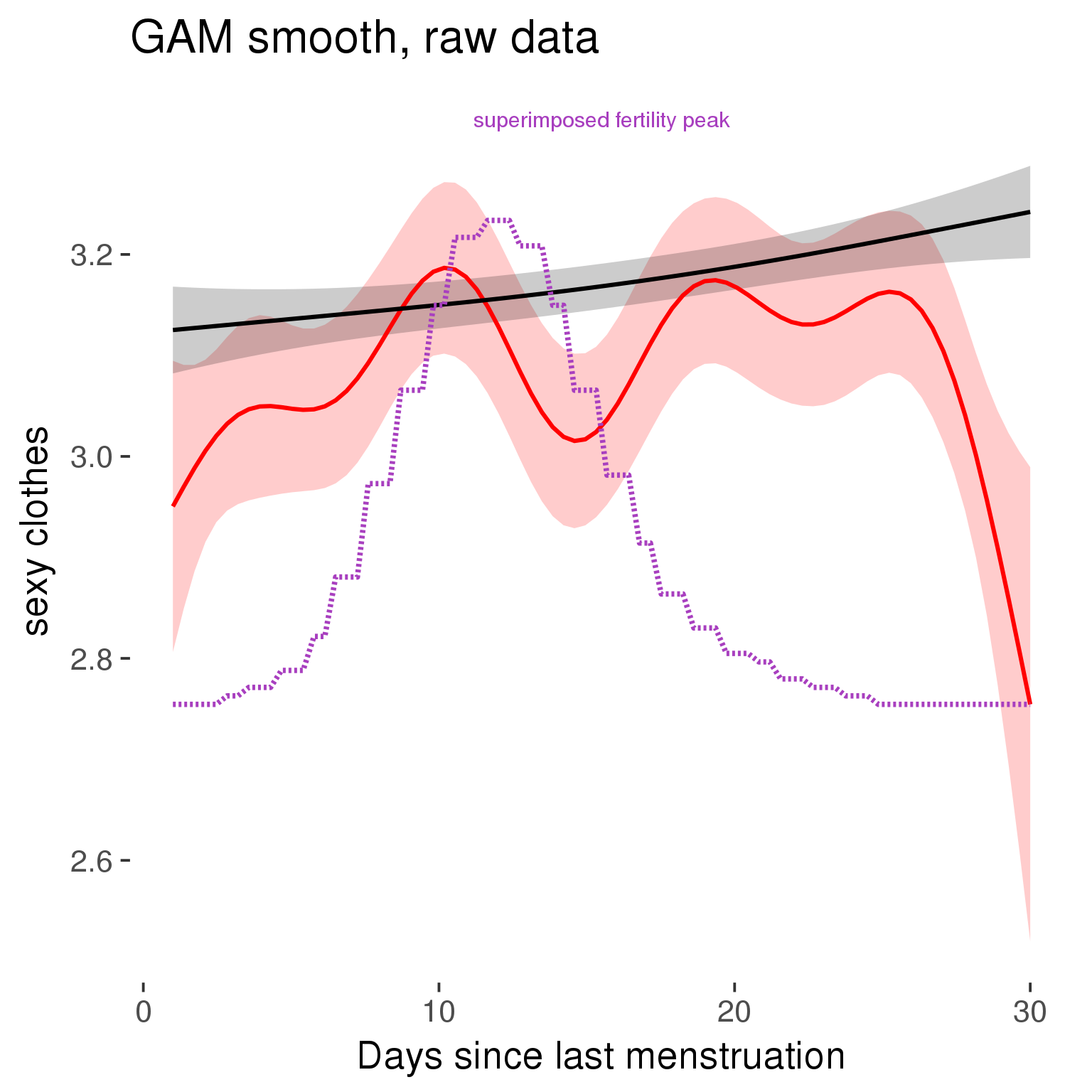
Means and standard errors over raw data
Nothing partialled out, just straight means with bootstrapped confidence intervals.
tryCatch({
trend_plot = ggplot(tmp,aes_string(x = "RCD", y = outcome, colour = "included")) +
geom_pointrange(size = 0.8, stat = 'summary', fun.data = "mean_cl_boot")
}, error = function(e){cat_message(e, "danger")})
tryCatch({
trend_data = ggplot_build(trend_plot)$data[[1]]
}, error = function(e){cat_message(e, "danger")})
trend_data$RCD = round(trend_data$x)
trend_data = left_join(trend_data, tmp %>% select(real, RCD,fertile) %>% unique(), by = "RCD")
trend_data %>%
filter(real == TRUE) %>%
mutate(superimposed = ( ( (fertile - 0.01)/0.58) * (max(y)-min(y) ) ) + min(y) ) ->
trend_data
plot3 = ggplot(trend_data) +
geom_pointrange(aes(x = x, y = y, ymin = ymin,ymax = ymax, colour = factor(group)), size = 0.8, stat = "identity", alpha = 0.6, position = position_dodge(width = .5)) +
scale_x_continuous("Days until next menstruation") +
geom_line(aes(x= x, y = superimposed), color = "#a83fbf", size = 1, linetype = 'dashed') +
annotate("text",x = mean(trend_data$x), y = max(trend_data$superimposed,na.rm=T) + 0.1, label = 'superimposed fertility peak', color = "#a83fbf") +
scale_y_continuous(outcome_label) +
ggtitle("Means with standard errors, raw data") +
scale_color_manual("Contraception status",values = c("2"="black","1"= "red"), labels = c("2"="hormonally\ncontracepting","1"="cycling"), guide = F) +
scale_fill_manual("Contraception status",values = c("2"="black","1"= "red"), labels = c("2"="hormonally\ncontracepting","1"="cycling"), guide = F)
suppressWarnings(print(plot3))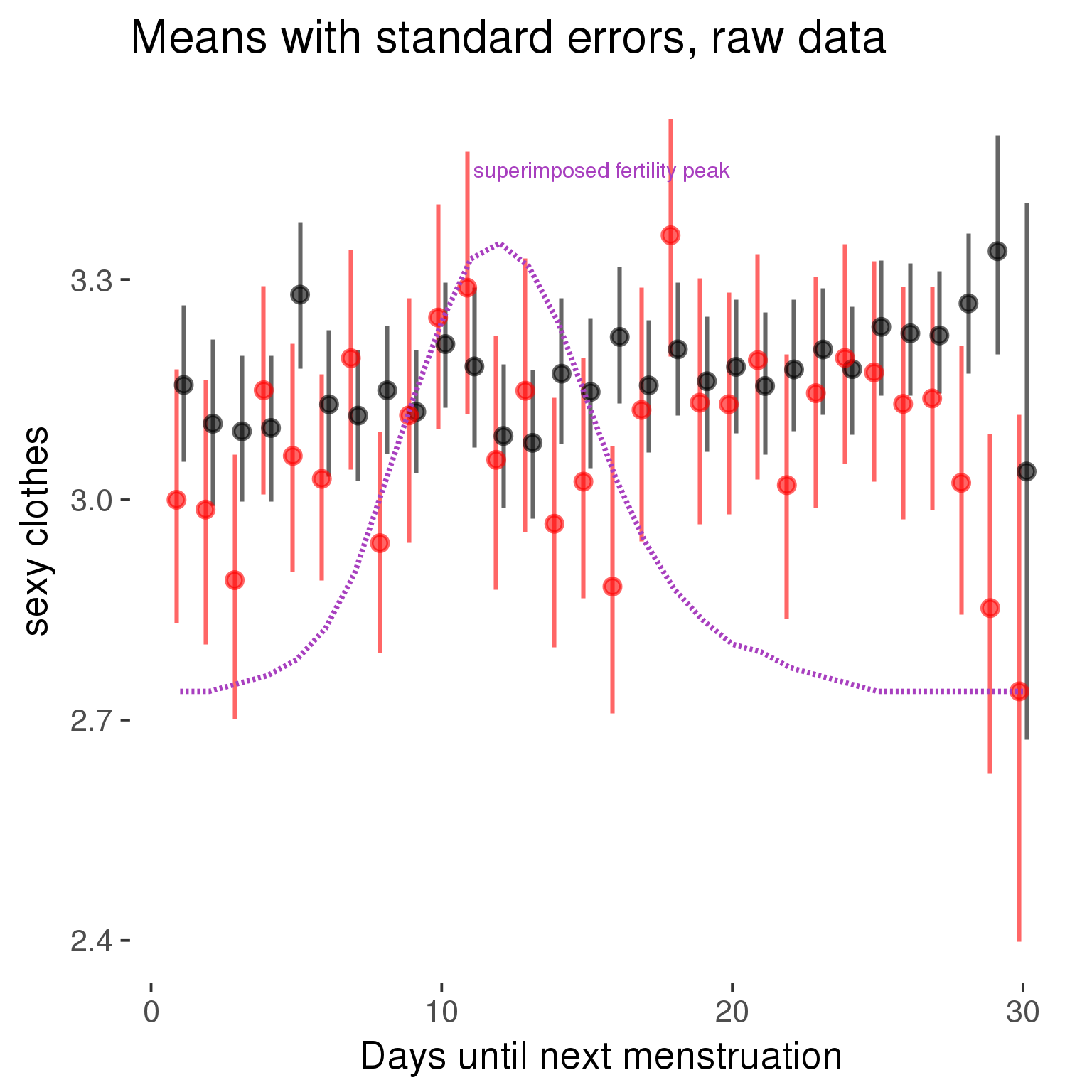
Robustness checks
M_r1: Random slopes for conception risk and menstruation
tryCatch({
# refit model with random effects for fertile and menstruation dummies
with_ind_diff = update(model, formula = . ~ . - (1| person) + (1 + fertile + menstruation | person))
# pull the random effects, format as tibble
rand = coef(with_ind_diff)$person %>%
tibble::rownames_to_column("person") %>%
mutate(person = as.numeric(person))
# pull the fixed effects
fixd = data.frame(fixef(with_ind_diff)) %>%
tibble::rownames_to_column("effect")
names(fixd) = c("effect", "pop_effect_size")
# pull apart the coefficients so that we can account for the fact that the random effect variation implicitly includes HC explaining the mean population-level effect of fertile/menstruation dummies among HC users
fixd = fixd %>%
separate(effect, c("included", "effect"), sep = ":", fill = "left") %>%
mutate(included = if_else(is.na(included), "cycling", str_replace(included, "included", "")))
fixd[2,c("included", "effect")] = c("horm_contra", "(Intercept)")
rand = rand %>%
# merge diary data on the random effects, so that we know who is a HC users and who isn't
inner_join(diary %>% select(person, included) %>% unique(), by = 'person') %>%
# gather into long format, to have the dataset by predictor
gather(effect, value, -person, -included) %>%
inner_join(fixd, by = c('effect', 'included')) %>%
# pull the fixed effects
mutate(
# only for those who are HC users, add the moderated population effect size for this effect (the random effects have the reference category mean)
value = if_else(included == "horm_contra", value + pop_effect_size, value),
effect = recode(effect, "includedhorm_contra" = "HC user",
"includedhorm_contra:fertile" = "HC user x fertile",
"includedhorm_contra:menstruationpre" = "HC user x premens.",
"includedhorm_contra:menstruationyes" = "HC user x mens.",
"menstruationyes" = "mens.",
"menstruationpre" = "premens.")) %>%
group_by(included, effect) %>%
# filter out predictors that aren't modelled as varying/random
filter(sd(value) > 0)
# plot dot plot of random effects
print(
ggplot(rand, aes(x = included, y = value, color = included, fill = included)) +
facet_wrap( ~ effect, scales = "free") +
# geom_violin(alpha = 0.4, size = 0) +
geom_dotplot(binaxis='y', dotsize = 0.1, method = "histodot") +
# geom_jitter(alpha = 0.05) +
coord_flip() +
geom_pointrange(stat = 'summary', fun.data = 'mean_sdl', color = 'darkred', size = 1.2) +
scale_color_manual("Contraception status", values = c("horm_contra"="black","cycling"= "red"), labels = c("horm_contra"="hormonally\ncontracepting","cycling"="cycling"), guide = F) +
scale_fill_manual("Contraception status", values = c("horm_contra"="black","cycling"= "red"), labels = c("horm_contra"="hormonally\ncontracepting","1"="cycling"), guide = F) +
ggtitle("M_r1: allowing participant-varying slopes", subtitle = "for the conception risk measure and the menstruation dummies") +
scale_x_discrete("Hormonal contraception", breaks = c("horm_contra", "cycling"), labels = c("yes", "no")) +
scale_y_continuous("Random effect size distribution"))
print_summary(with_ind_diff)
cat(pander(anova(model, with_ind_diff)))
}, error = function(e){
with_ind_diff = model
cat_message(e, "danger")
})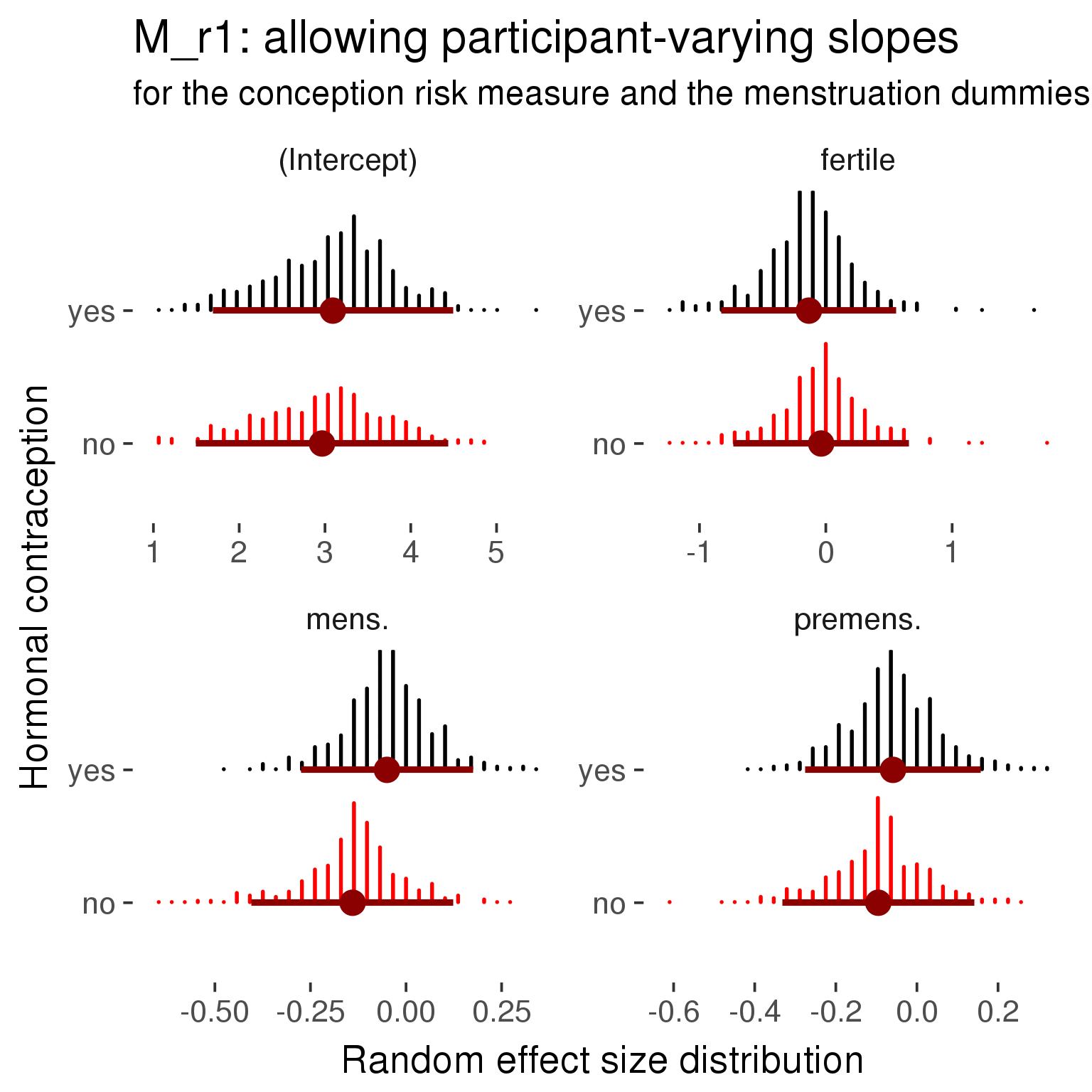
Linear mixed model fit by REML ['lmerMod']
Formula: sexy_clothes ~ included + menstruation + fertile + fertile_mean +
(1 + fertile + menstruation | person) + included:menstruation + included:fertile
Data: diary
REML criterion at convergence: 75718
Scaled residuals:
Min 1Q Median 3Q Max
-4.158 -0.602 -0.015 0.604 4.476
Random effects:
Groups Name Variance Std.Dev. Corr
person (Intercept) 0.5986 0.774
fertile 0.4815 0.694 -0.16
menstruationpre 0.0717 0.268 -0.07 0.41
menstruationyes 0.0773 0.278 -0.16 0.24 0.61
Residual 0.8749 0.935
Number of obs: 26688, groups: person, 1054
Fixed effects:
Estimate Std. Error t value
(Intercept) 2.9656 0.0675 43.9
includedhorm_contra 0.1258 0.0556 2.3
menstruationpre -0.0953 0.0327 -2.9
menstruationyes -0.1398 0.0315 -4.4
fertile -0.0369 0.0702 -0.5
fertile_mean 0.5933 0.3103 1.9
includedhorm_contra:menstruationpre 0.0362 0.0419 0.9
includedhorm_contra:menstruationyes 0.0899 0.0410 2.2
includedhorm_contra:fertile -0.0969 0.0892 -1.1
Correlation of Fixed Effects:
(Intr) incld_ mnstrtnp mnstrtny fertil frtl_m inclddhrm_cntr:mnstrtnp
inclddhrm_c -0.476
menstrutnpr -0.165 0.212
menstrutnys -0.188 0.230 0.444
fertile -0.172 0.281 0.444 0.343
fertile_men -0.769 -0.027 -0.012 -0.001 -0.076
inclddhrm_cntr:mnstrtnp 0.138 -0.265 -0.779 -0.346 -0.345 -0.003
inclddhrm_cntr:mnstrtny 0.149 -0.284 -0.340 -0.766 -0.262 -0.005 0.432
inclddhrm_cntr:f 0.172 -0.355 -0.349 -0.270 -0.784 0.012 0.443
inclddhrm_cntr:mnstrtny
inclddhrm_c
menstrutnpr
menstrutnys
fertile
fertile_men
inclddhrm_cntr:mnstrtnp
inclddhrm_cntr:mnstrtny
inclddhrm_cntr:f 0.339
refitting model(s) with ML (instead of REML)
| Df | AIC | BIC | logLik | deviance | Chisq | Chi Df | Pr(>Chisq) | |
|---|---|---|---|---|---|---|---|---|
| object | 11 | 75832 | 75922 | -37905 | 75810 | NA | NA | NA |
| ..1 | 20 | 75719 | 75882 | -37839 | 75679 | 131.1 | 9 | 7e-24 |
robustness_check_ovu_shift(model, diary)M_e: Exclusion criteria
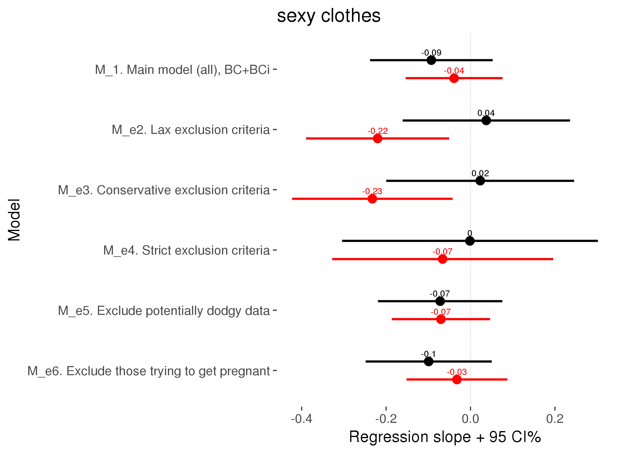
M_p: Predictors
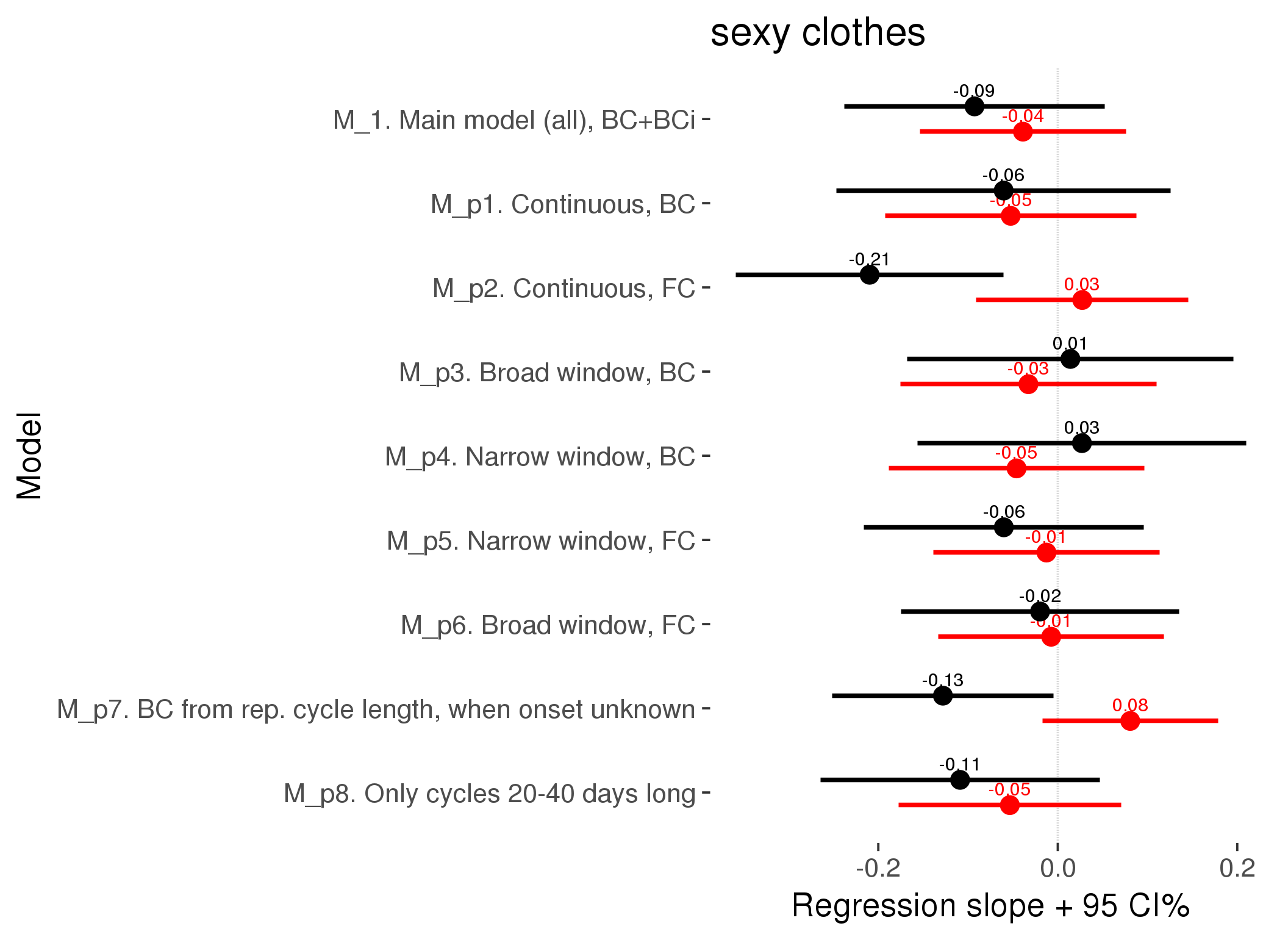
M_c: Covariates, controls, autocorrelation
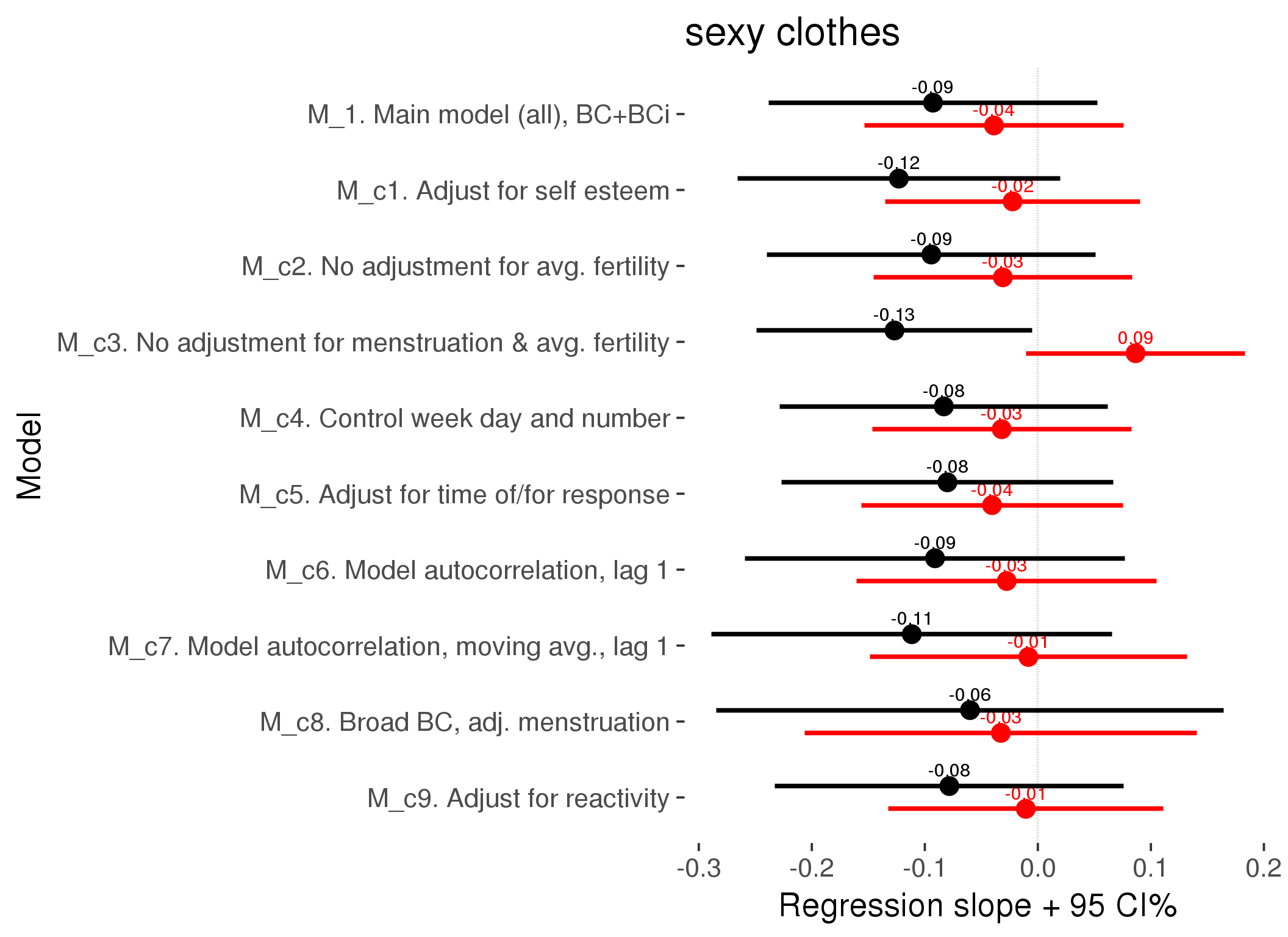
Linear mixed model fit by REML ['lmerMod']
REML criterion at convergence: 69320
Scaled residuals:
Min 1Q Median 3Q Max
-4.294 -0.606 -0.016 0.614 4.479
Random effects:
Groups Name Variance Std.Dev.
person (Intercept) 0.576 0.759
Xr.2 s(days_filled_out):includedhorm_contra 0.000 0.000
Xr.1 s(days_filled_out):includedcycling 0.000 0.000
Xr.0 s(day_number):includedhorm_contra 0.144 0.379
Xr s(day_number):includedcycling 0.000 0.000
Residual 0.898 0.948
Number of obs: 24384, groups: person, 1054; Xr.2, 8; Xr.1, 8; Xr.0, 8; Xr, 8
Fixed effects:
Estimate Std. Error t value
X(Intercept) 2.9843 0.0671 44.5
Xincludedhorm_contra 0.1179 0.0554 2.1
Xmenstruationpre -0.0894 0.0302 -3.0
Xmenstruationyes -0.1276 0.0290 -4.4
Xfertile -0.0106 0.0622 -0.2
Xfertile_mean 0.5681 0.3065 1.9
Xincludedhorm_contra:menstruationpre 0.0400 0.0388 1.0
Xincludedhorm_contra:menstruationyes 0.0828 0.0380 2.2
Xincludedhorm_contra:fertile -0.0783 0.0787 -1.0
Xs(day_number):includedcyclingFx1 -0.0552 0.0482 -1.1
Xs(day_number):includedhorm_contraFx1 0.0872 0.0905 1.0
Xs(days_filled_out):includedcyclingFx1 0.1172 0.0498 2.4
Xs(days_filled_out):includedhorm_contraFx1 0.0542 0.0427 1.3
Family: gaussian
Link function: identity
Formula:
sexy_clothes ~ included + menstruation + fertile + fertile_mean +
s(day_number, by = included) + s(days_filled_out, by = included) +
included:menstruation + included:fertile
Parametric coefficients:
Estimate Std. Error t value Pr(>|t|)
(Intercept) 2.9843 0.0671 44.46 < 2e-16 ***
includedhorm_contra 0.1179 0.0554 2.13 0.0332 *
menstruationpre -0.0894 0.0302 -2.96 0.0031 **
menstruationyes -0.1276 0.0290 -4.40 0.000011 ***
fertile -0.0106 0.0622 -0.17 0.8641
fertile_mean 0.5681 0.3065 1.85 0.0639 .
includedhorm_contra:menstruationpre 0.0400 0.0388 1.03 0.3026
includedhorm_contra:menstruationyes 0.0828 0.0380 2.18 0.0294 *
includedhorm_contra:fertile -0.0783 0.0787 -0.99 0.3199
---
Signif. codes: 0 '***' 0.001 '**' 0.01 '*' 0.05 '.' 0.1 ' ' 1
Approximate significance of smooth terms:
edf Ref.df F p-value
s(day_number):includedcycling 1.00 1.00 1.31 0.252
s(day_number):includedhorm_contra 5.05 5.05 8.68 0.000000027 ***
s(days_filled_out):includedcycling 1.00 1.00 5.54 0.019 *
s(days_filled_out):includedhorm_contra 1.00 1.00 1.61 0.204
---
Signif. codes: 0 '***' 0.001 '**' 0.01 '*' 0.05 '.' 0.1 ' ' 1
R-sq.(adj) = 0.00585
lmer.REML = 69320 Scale est. = 0.89842 n = 24384
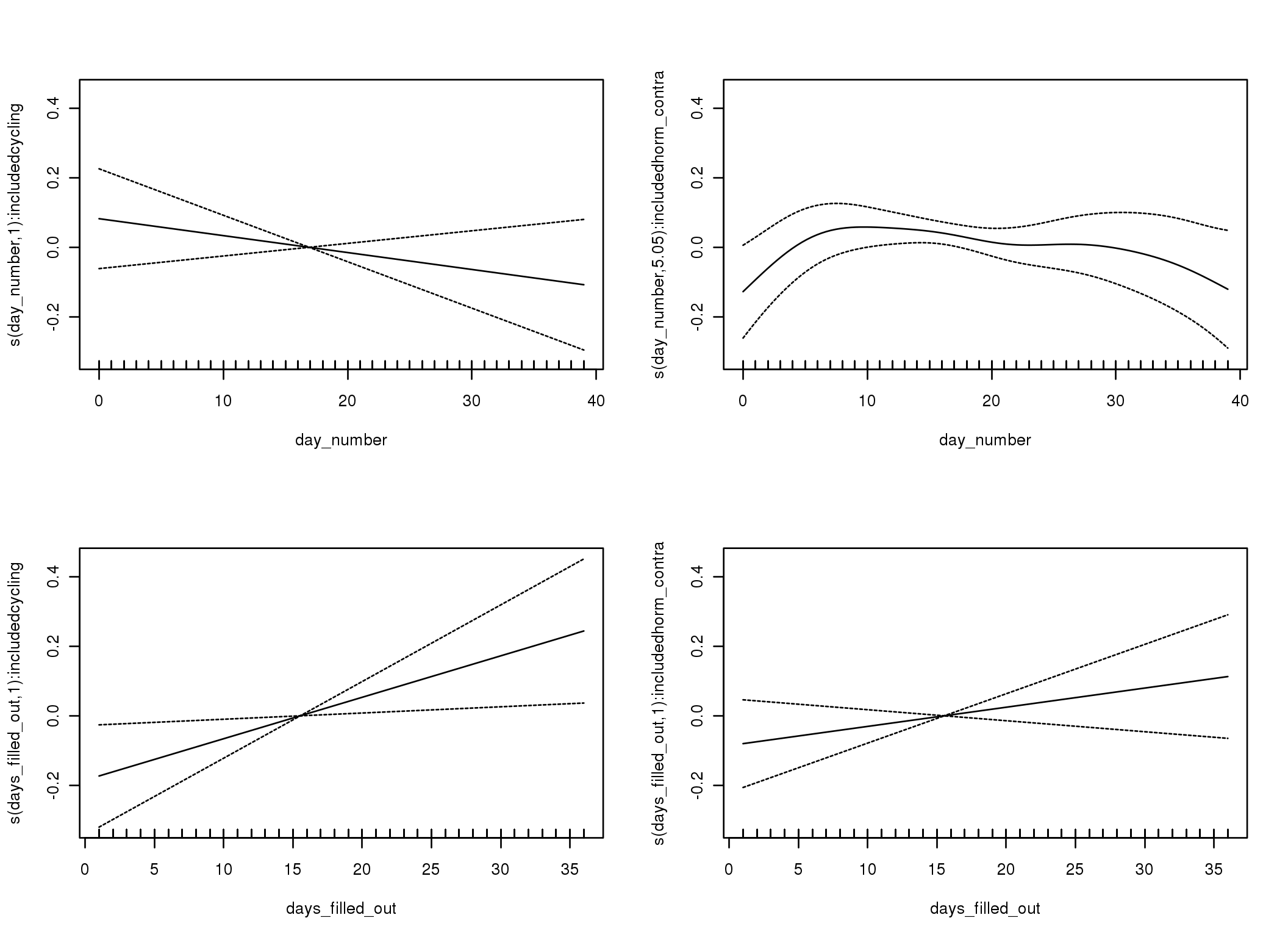
Linear mixed-effects model fit by REML
Data: diary
AIC BIC logLik
75005 75103 -37491
Random effects:
Formula: ~1 | person
(Intercept) Residual
StdDev: 0.7509 0.959
Correlation Structure: ARMA(1,0)
Formula: ~day_number | person
Parameter estimate(s):
Phi1
0.2144
Fixed effects: sexy_clothes ~ included * (menstruation + fertile) + fertile_mean
Value Std.Error DF t-value p-value
(Intercept) 2.9653 0.06779 25628 43.74 0.0000
includedhorm_contra 0.1225 0.05575 1051 2.20 0.0282
menstruationpre -0.0866 0.03250 25628 -2.66 0.0077
menstruationyes -0.1380 0.03040 25628 -4.54 0.0000
fertile -0.0276 0.06773 25628 -0.41 0.6838
fertile_mean 0.6086 0.31121 1051 1.96 0.0508
includedhorm_contra:menstruationpre 0.0320 0.04173 25628 0.77 0.4436
includedhorm_contra:menstruationyes 0.0851 0.03971 25628 2.14 0.0320
includedhorm_contra:fertile -0.0910 0.08570 25628 -1.06 0.2884
Correlation:
(Intr) incld_ mnstrtnp mnstrtny fertil frtl_m inclddhrm_cntr:mnstrtnp
includedhorm_contra -0.476
menstruationpre -0.184 0.231
menstruationyes -0.179 0.224 0.400
fertile -0.176 0.290 0.442 0.369
fertile_mean -0.769 -0.027 -0.008 -0.005 -0.079
includedhorm_contra:menstruationpre 0.151 -0.288 -0.779 -0.311 -0.343 -0.004
includedhorm_contra:menstruationyes 0.144 -0.274 -0.306 -0.766 -0.282 -0.004 0.385
includedhorm_contra:fertile 0.177 -0.366 -0.349 -0.292 -0.786 0.013 0.441
inclddhrm_cntr:mnstrtny
includedhorm_contra
menstruationpre
menstruationyes
fertile
fertile_mean
includedhorm_contra:menstruationpre
includedhorm_contra:menstruationyes
includedhorm_contra:fertile 0.364
Standardized Within-Group Residuals:
Min Q1 Med Q3 Max
-4.10600 -0.60144 -0.02197 0.61500 4.40797
Number of Observations: 26688
Number of Groups: 1054
Linear mixed-effects model fit by REML
Data: diary
AIC BIC logLik
74823 74930 -37399
Random effects:
Formula: ~1 | person
(Intercept) Residual
StdDev: 0.7363 0.968
Correlation Structure: ARMA(1,1)
Formula: ~day_number | person
Parameter estimate(s):
Phi1 Theta1
0.6705 -0.4803
Fixed effects: sexy_clothes ~ included * (menstruation + fertile) + fertile_mean
Value Std.Error DF t-value p-value
(Intercept) 2.9588 0.06796 25628 43.54 0.0000
includedhorm_contra 0.1276 0.05593 1051 2.28 0.0227
menstruationpre -0.0736 0.03312 25628 -2.22 0.0263
menstruationyes -0.1328 0.03137 25628 -4.23 0.0000
fertile -0.0084 0.07162 25628 -0.12 0.9066
fertile_mean 0.6053 0.31261 1051 1.94 0.0531
includedhorm_contra:menstruationpre 0.0175 0.04257 25628 0.41 0.6804
includedhorm_contra:menstruationyes 0.0741 0.04083 25628 1.82 0.0695
includedhorm_contra:fertile -0.1116 0.09051 25628 -1.23 0.2178
Correlation:
(Intr) incld_ mnstrtnp mnstrtny fertil frtl_m inclddhrm_cntr:mnstrtnp
includedhorm_contra -0.476
menstruationpre -0.185 0.229
menstruationyes -0.185 0.230 0.420
fertile -0.177 0.296 0.395 0.355
fertile_mean -0.769 -0.028 -0.005 -0.005 -0.084
includedhorm_contra:menstruationpre 0.150 -0.286 -0.778 -0.327 -0.306 -0.004
includedhorm_contra:menstruationyes 0.148 -0.281 -0.323 -0.768 -0.272 -0.003 0.408
includedhorm_contra:fertile 0.180 -0.374 -0.312 -0.281 -0.787 0.014 0.394
inclddhrm_cntr:mnstrtny
includedhorm_contra
menstruationpre
menstruationyes
fertile
fertile_mean
includedhorm_contra:menstruationpre
includedhorm_contra:menstruationyes
includedhorm_contra:fertile 0.349
Standardized Within-Group Residuals:
Min Q1 Med Q3 Max
-4.00489 -0.60384 -0.01575 0.62031 4.28612
Number of Observations: 26688
Number of Groups: 1054
M_d: Other designs
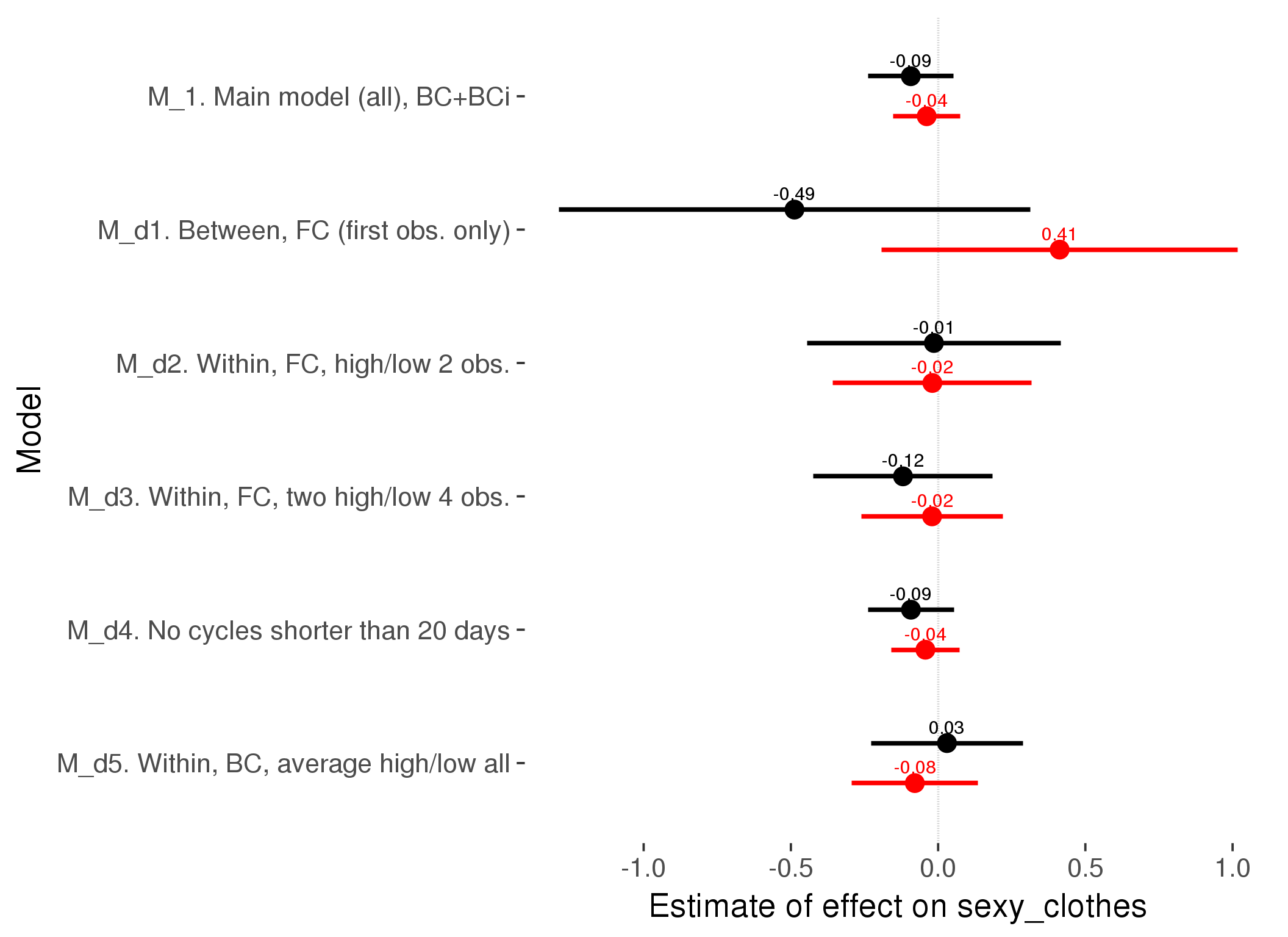
M_m1: Moderation by contraceptive method
Based on the sample with lax exclusion criteria. Users who used any hormonal contraception are classified as hormonal, users who use any awareness-based methods (counting, temperature-based) are classified as ‘fertility-awareness’, women who don’t fall into the before groups and use condoms, pessars, coitus interruptus etc. are classified as ‘barrie or abstinence’. Women who don’t use contraception or use other methods such as sterilisation are excluded from this analysis.
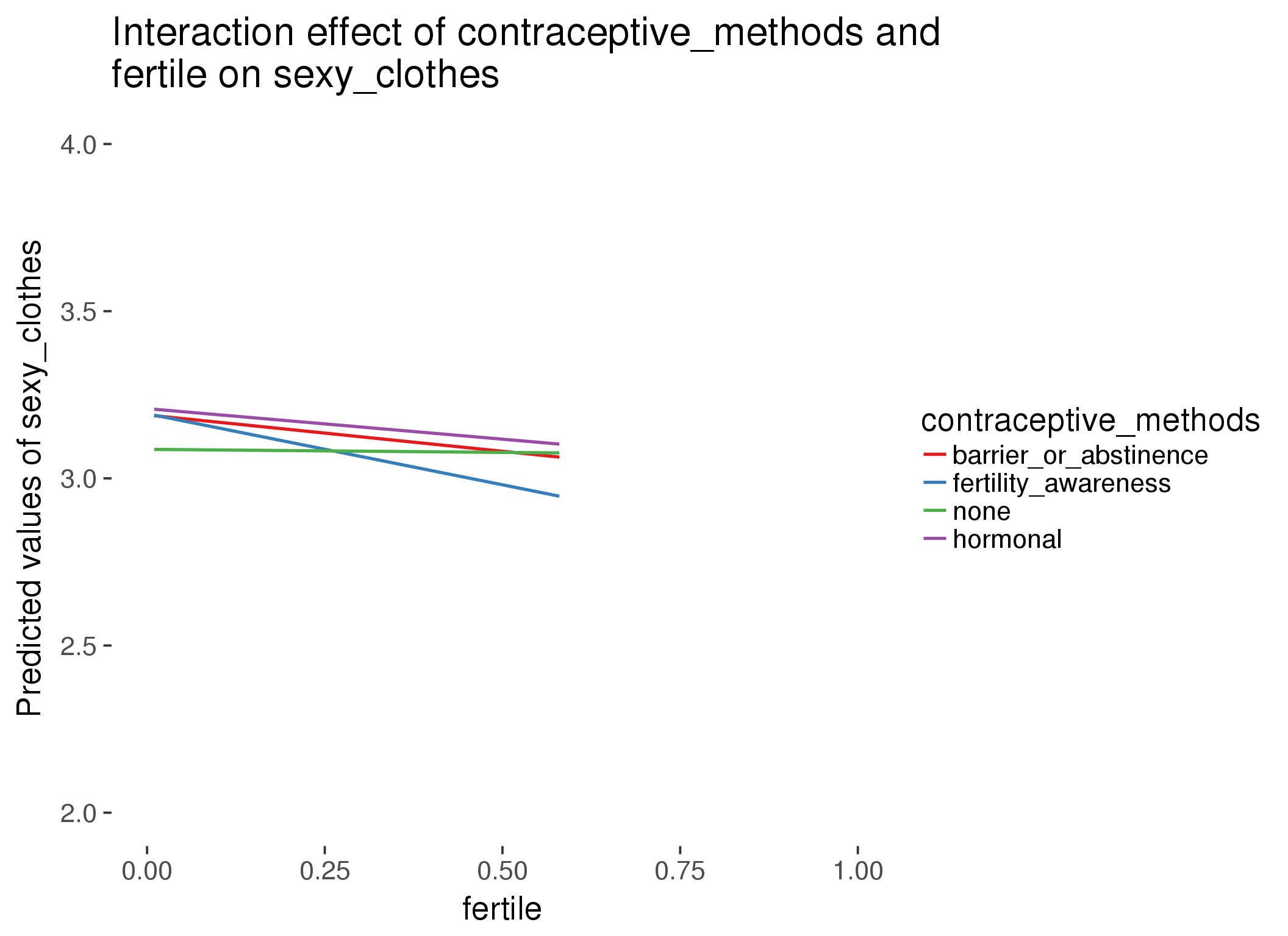
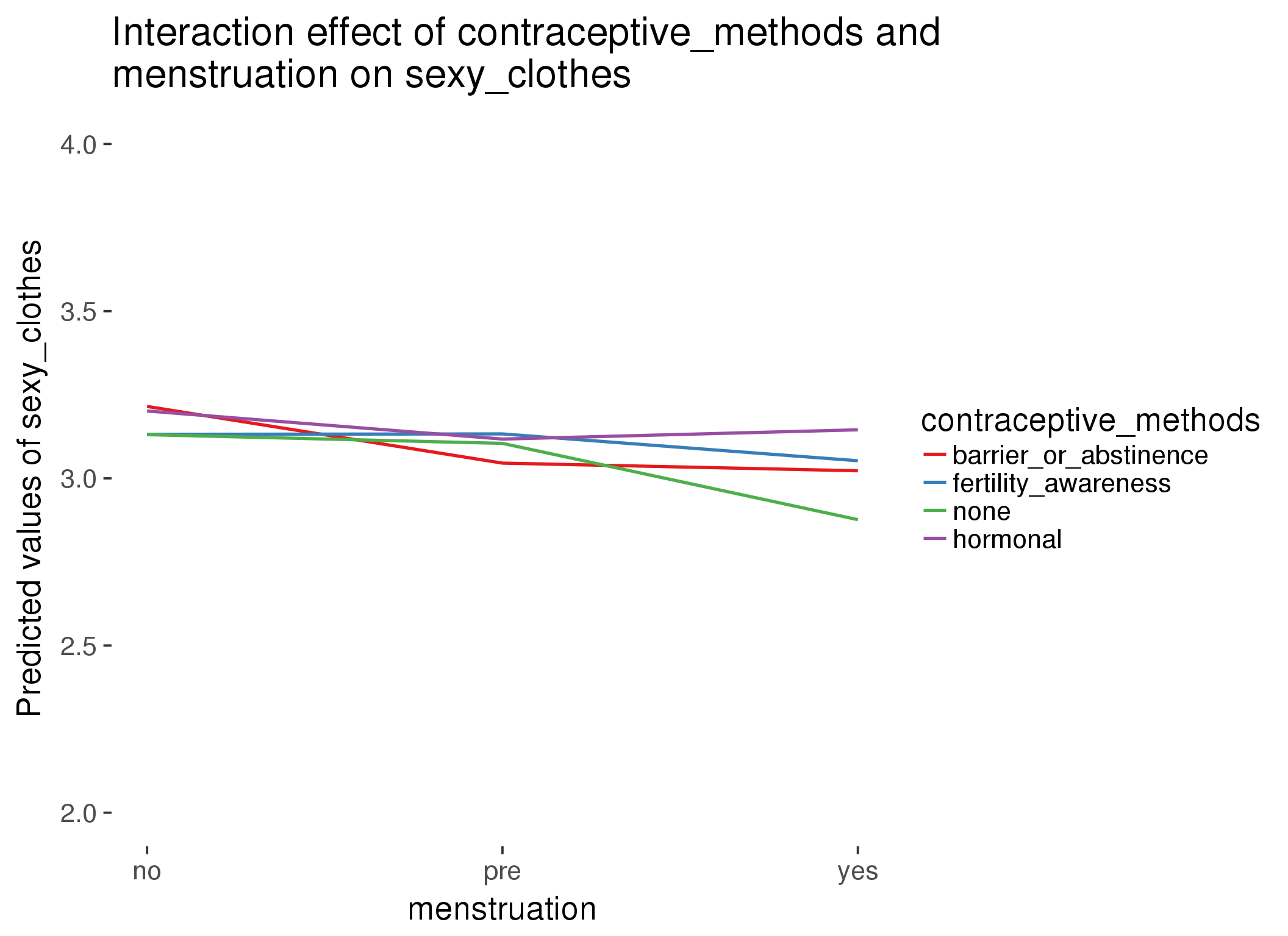
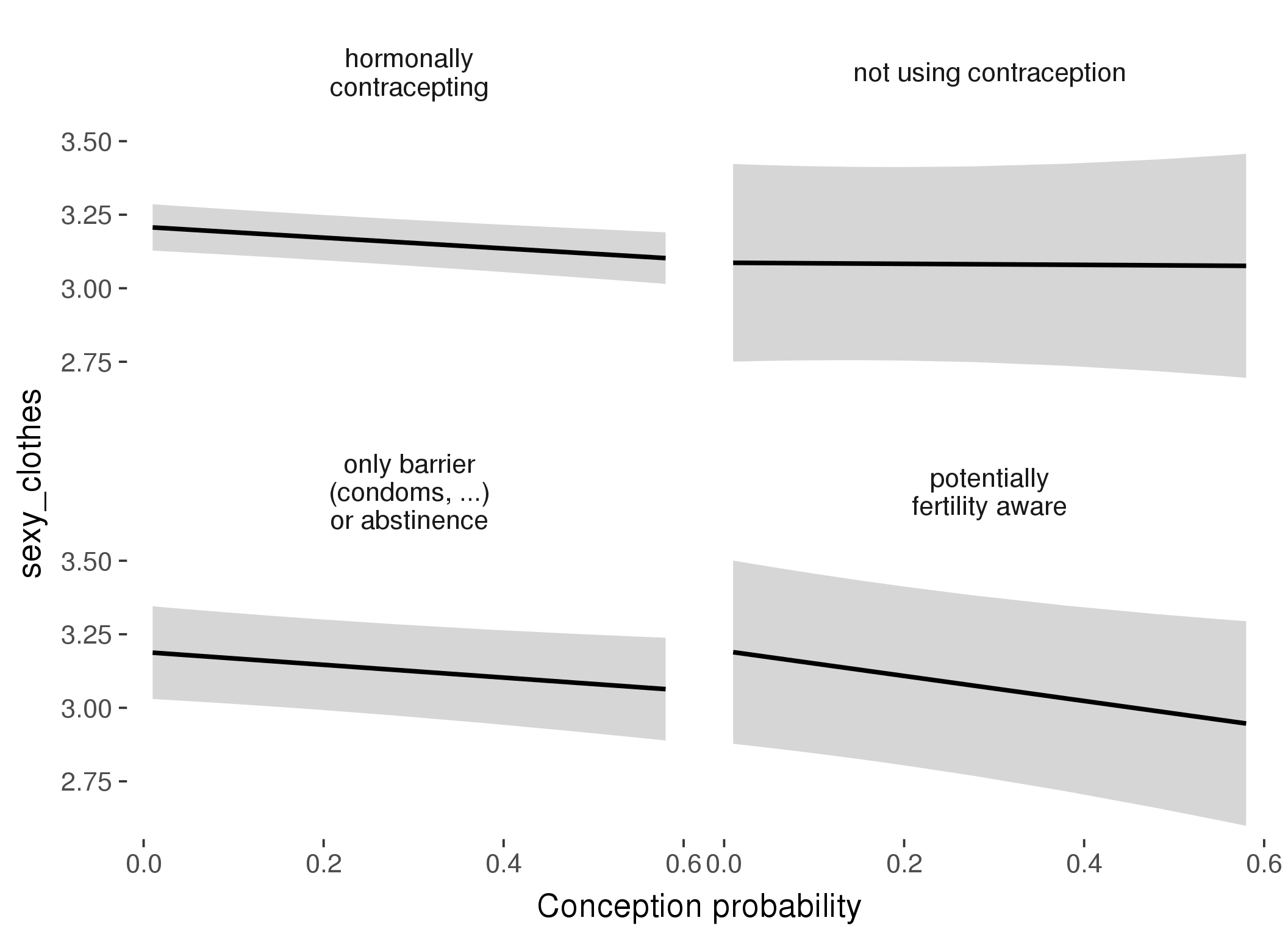
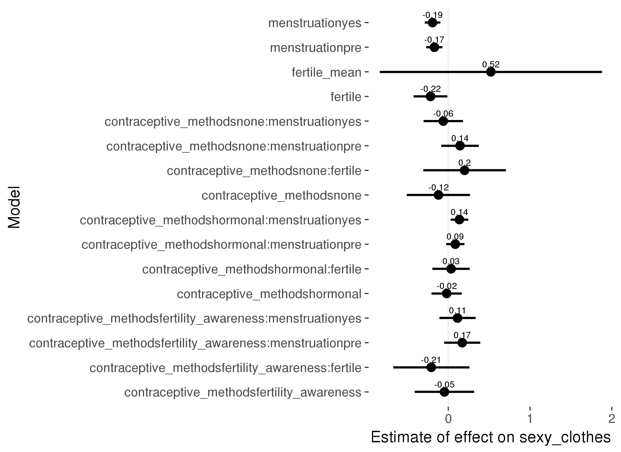
Linear mixed model fit by REML ['lmerMod']
Formula: sexy_clothes ~ fertile_mean + (1 | person) + contraceptive_methods +
fertile + menstruation + fertile:contraceptive_methods + menstruation:contraceptive_methods
Data: diary
Subset: !is.na(included_lax) & contraceptive_method != "other"
REML criterion at convergence: 47798
Scaled residuals:
Min 1Q Median 3Q Max
-4.158 -0.612 -0.013 0.617 4.193
Random effects:
Groups Name Variance Std.Dev.
person (Intercept) 0.549 0.741
Residual 0.882 0.939
Number of obs: 17031, groups: person, 513
Fixed effects:
Estimate Std. Error t value
(Intercept) 3.1618 0.1428 22.14
fertile_mean 0.5211 0.6937 0.75
contraceptive_methodsfertility_awareness -0.0469 0.1861 -0.25
contraceptive_methodsnone -0.1194 0.1973 -0.61
contraceptive_methodshormonal -0.0197 0.0938 -0.21
fertile -0.2175 0.1048 -2.08
menstruationpre -0.1696 0.0506 -3.35
menstruationyes -0.1925 0.0483 -3.98
contraceptive_methodsfertility_awareness:fertile -0.2080 0.2379 -0.87
contraceptive_methodsnone:fertile 0.1993 0.2576 0.77
contraceptive_methodshormonal:fertile 0.0346 0.1170 0.30
contraceptive_methodsfertility_awareness:menstruationpre 0.1708 0.1121 1.52
contraceptive_methodsnone:menstruationpre 0.1436 0.1172 1.22
contraceptive_methodshormonal:menstruationpre 0.0856 0.0570 1.50
contraceptive_methodsfertility_awareness:menstruationyes 0.1134 0.1127 1.01
contraceptive_methodsnone:menstruationyes -0.0617 0.1225 -0.50
contraceptive_methodshormonal:menstruationyes 0.1363 0.0551 2.47
refitting model(s) with ML (instead of REML)
| Df | AIC | BIC | logLik | deviance | Chisq | Chi Df | Pr(>Chisq) | |
|---|---|---|---|---|---|---|---|---|
| add_main | 13 | 47782 | 47883 | -23878 | 47756 | NA | NA | NA |
| by_method | 19 | 47784 | 47931 | -23873 | 47746 | 10.17 | 6 | 0.1175 |
M_m2: Moderation by participant age
model %>%
test_moderator("age_group", diary, xlevels = 5)refitting model(s) with ML (instead of REML)
| Df | AIC | BIC | logLik | deviance | Chisq | Chi Df | Pr(>Chisq) | |
|---|---|---|---|---|---|---|---|---|
| with_main | 19 | 75814 | 75970 | -37888 | 75776 | NA | NA | NA |
| with_mod | 27 | 75816 | 76037 | -37881 | 75762 | 14.18 | 8 | 0.07712 |
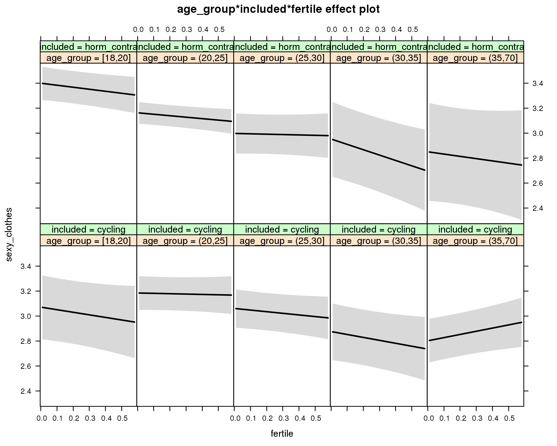
Linear mixed model fit by REML ['lmerMod']
Formula: sexy_clothes ~ menstruation + fertile_mean + (1 | person) + age_group +
included + fertile + menstruation:included + age_group:included +
age_group:fertile + included:fertile + age_group:included:fertile
Data: diary
REML criterion at convergence: 75839
Scaled residuals:
Min 1Q Median 3Q Max
-4.229 -0.607 -0.017 0.615 4.566
Random effects:
Groups Name Variance Std.Dev.
person (Intercept) 0.568 0.753
Residual 0.904 0.951
Number of obs: 26688, groups: person, 1054
Fixed effects:
Estimate Std. Error t value
(Intercept) 3.0111 0.1384 21.76
menstruationpre -0.0948 0.0290 -3.27
menstruationyes -0.1447 0.0274 -5.29
fertile_mean 0.5849 0.3055 1.91
age_group(20,25] 0.1134 0.1480 0.77
age_group(25,30] -0.0105 0.1523 -0.07
age_group(30,35] -0.1955 0.1748 -1.12
age_group(35,70] -0.2696 0.1583 -1.70
includedhorm_contra 0.3073 0.1483 2.07
fertile -0.2059 0.1675 -1.23
menstruationpre:includedhorm_contra 0.0349 0.0373 0.94
menstruationyes:includedhorm_contra 0.0898 0.0359 2.50
age_group(20,25]:includedhorm_contra -0.3502 0.1687 -2.08
age_group(25,30]:includedhorm_contra -0.3916 0.1859 -2.11
age_group(30,35]:includedhorm_contra -0.2513 0.2419 -1.04
age_group(35,70]:includedhorm_contra -0.2797 0.2644 -1.06
age_group(20,25]:fertile 0.1768 0.1855 0.95
age_group(25,30]:fertile 0.0759 0.1912 0.40
age_group(30,35]:fertile -0.0292 0.2214 -0.13
age_group(35,70]:fertile 0.4604 0.1998 2.30
includedhorm_contra:fertile 0.0445 0.1857 0.24
age_group(20,25]:includedhorm_contra:fertile -0.1329 0.2078 -0.64
age_group(25,30]:includedhorm_contra:fertile 0.0553 0.2302 0.24
age_group(30,35]:includedhorm_contra:fertile -0.2392 0.2972 -0.80
age_group(35,70]:includedhorm_contra:fertile -0.4815 0.3376 -1.43
M_m3: Moderation by weekend
model %>%
test_moderator("weekend", diary, xlevels = 2) refitting model(s) with ML (instead of REML)
| Df | AIC | BIC | logLik | deviance | Chisq | Chi Df | Pr(>Chisq) | |
|---|---|---|---|---|---|---|---|---|
| with_main | 13 | 75831 | 75937 | -37902 | 75805 | NA | NA | NA |
| with_mod | 15 | 75832 | 75955 | -37901 | 75802 | 2.048 | 2 | 0.3592 |
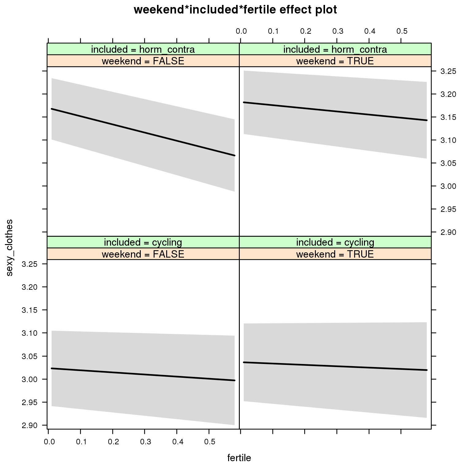
Linear mixed model fit by REML ['lmerMod']
Formula: sexy_clothes ~ menstruation + fertile_mean + (1 | person) + weekend +
included + fertile + menstruation:included + weekend:included +
weekend:fertile + included:fertile + weekend:included:fertile
Data: diary
REML criterion at convergence: 75862
Scaled residuals:
Min 1Q Median 3Q Max
-4.190 -0.607 -0.018 0.617 4.486
Random effects:
Groups Name Variance Std.Dev.
person (Intercept) 0.583 0.763
Residual 0.904 0.951
Number of obs: 26688, groups: person, 1054
Fixed effects:
Estimate Std. Error t value
(Intercept) 2.9586405 0.0677581 43.7
menstruationpre -0.0947965 0.0290194 -3.3
menstruationyes -0.1433143 0.0273429 -5.2
fertile_mean 0.6143382 0.3072696 2.0
weekendTRUE 0.0130163 0.0252898 0.5
includedhorm_contra 0.1239595 0.0564046 2.2
fertile -0.0457958 0.0712405 -0.6
menstruationpre:includedhorm_contra 0.0354614 0.0372531 1.0
menstruationyes:includedhorm_contra 0.0890829 0.0358424 2.5
weekendTRUE:includedhorm_contra 0.0000264 0.0325513 0.0
weekendTRUE:fertile 0.0163008 0.0980938 0.2
includedhorm_contra:fertile -0.1321367 0.0905065 -1.5
weekendTRUE:includedhorm_contra:fertile 0.0932567 0.1247604 0.7
M_m4: Moderation by weekday
model %>%
test_moderator("weekday", diary, xlevels = 7)refitting model(s) with ML (instead of REML)
| Df | AIC | BIC | logLik | deviance | Chisq | Chi Df | Pr(>Chisq) | |
|---|---|---|---|---|---|---|---|---|
| with_main | 23 | 75797 | 75986 | -37876 | 75751 | NA | NA | NA |
| with_mod | 35 | 75815 | 76102 | -37873 | 75745 | 5.728 | 12 | 0.9292 |
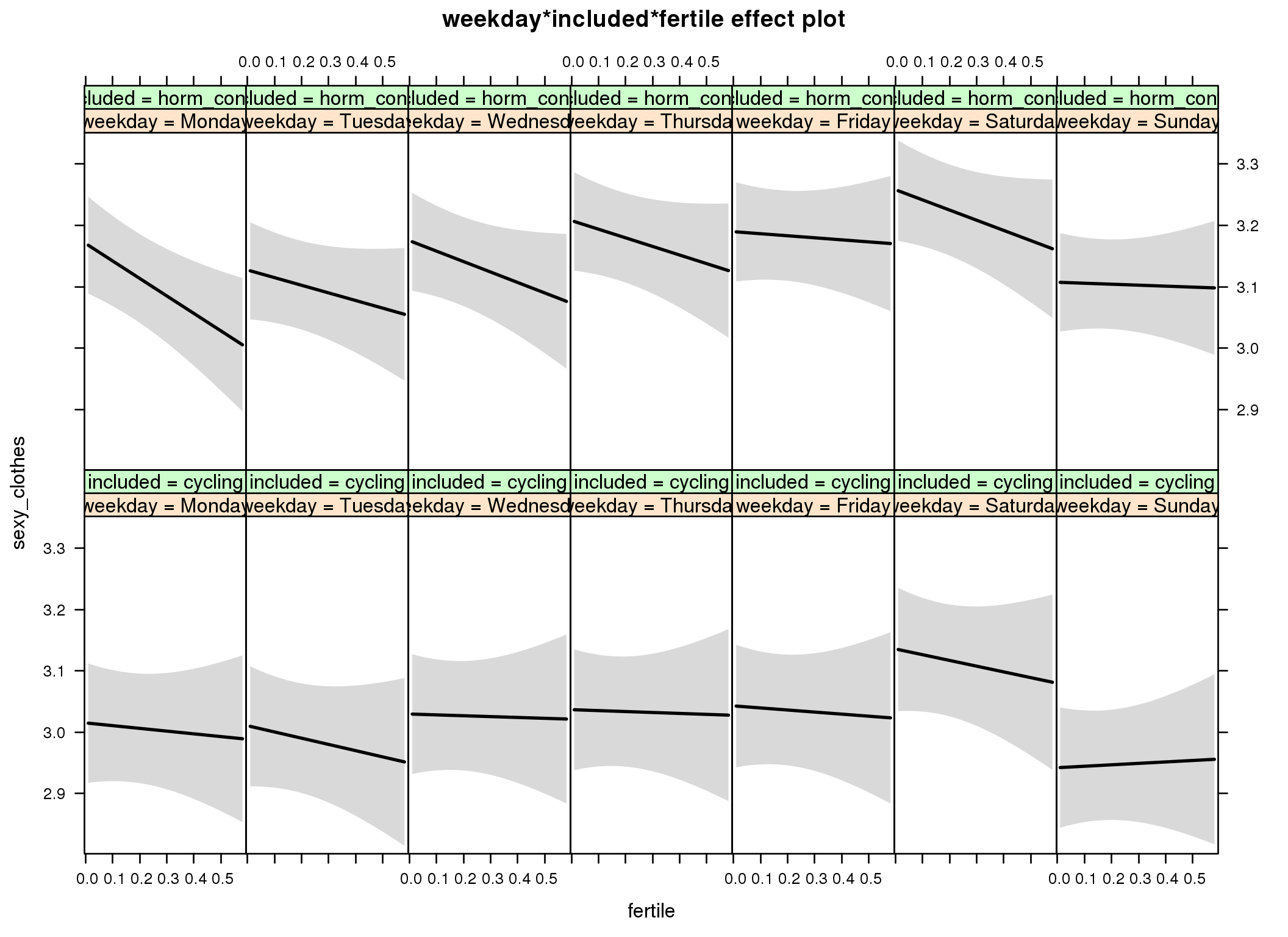
Linear mixed model fit by REML ['lmerMod']
Formula: sexy_clothes ~ menstruation + fertile_mean + (1 | person) + weekday +
included + fertile + menstruation:included + weekday:included +
weekday:fertile + included:fertile + weekday:included:fertile
Data: diary
REML criterion at convergence: 75878
Scaled residuals:
Min 1Q Median 3Q Max
-4.134 -0.608 -0.013 0.614 4.422
Random effects:
Groups Name Variance Std.Dev.
person (Intercept) 0.583 0.764
Residual 0.903 0.950
Number of obs: 26688, groups: person, 1054
Fixed effects:
Estimate Std. Error t value
(Intercept) 2.94865 0.07316 40.3
menstruationpre -0.09416 0.02900 -3.2
menstruationyes -0.14320 0.02733 -5.2
fertile_mean 0.62237 0.30726 2.0
weekdayTuesday -0.00465 0.04523 -0.1
weekdayWednesday 0.01445 0.04516 0.3
weekdayThursday 0.02157 0.04567 0.5
weekdayFriday 0.02773 0.04644 0.6
weekdaySaturday 0.12050 0.04690 2.6
weekdaySunday -0.07304 0.04533 -1.6
includedhorm_contra 0.13404 0.06651 2.0
fertile -0.04462 0.12739 -0.4
menstruationpre:includedhorm_contra 0.03398 0.03723 0.9
menstruationyes:includedhorm_contra 0.08795 0.03582 2.5
weekdayTuesday:includedhorm_contra -0.03865 0.05810 -0.7
weekdayWednesday:includedhorm_contra -0.00996 0.05830 -0.2
weekdayThursday:includedhorm_contra 0.01569 0.05885 0.3
weekdayFriday:includedhorm_contra -0.00852 0.05965 -0.1
weekdaySaturday:includedhorm_contra -0.03288 0.06036 -0.5
weekdaySunday:includedhorm_contra 0.00979 0.05850 0.2
weekdayTuesday:fertile -0.05707 0.17536 -0.3
weekdayWednesday:fertile 0.03064 0.17618 0.2
weekdayThursday:fertile 0.02925 0.17870 0.2
weekdayFriday:fertile 0.01102 0.17901 0.1
weekdaySaturday:fertile -0.04887 0.18139 -0.3
weekdaySunday:fertile 0.06814 0.17628 0.4
includedhorm_contra:fertile -0.24026 0.16294 -1.5
weekdayTuesday:includedhorm_contra:fertile 0.21756 0.22381 1.0
weekdayWednesday:includedhorm_contra:fertile 0.08386 0.22558 0.4
weekdayThursday:includedhorm_contra:fertile 0.11514 0.22739 0.5
weekdayFriday:includedhorm_contra:fertile 0.24060 0.22810 1.1
weekdaySaturday:includedhorm_contra:fertile 0.16785 0.23140 0.7
weekdaySunday:includedhorm_contra:fertile 0.20091 0.22517 0.9
M_m5: Moderation by exclusion threshold
model %>%
test_moderator("included_levels", diary, xlevels = 4)refitting model(s) with ML (instead of REML)
| Df | AIC | BIC | logLik | deviance | Chisq | Chi Df | Pr(>Chisq) | |
|---|---|---|---|---|---|---|---|---|
| with_main | 17 | 75835 | 75974 | -37900 | 75801 | NA | NA | NA |
| with_mod | 23 | 75823 | 76011 | -37888 | 75777 | 23.77 | 6 | 0.000576 |
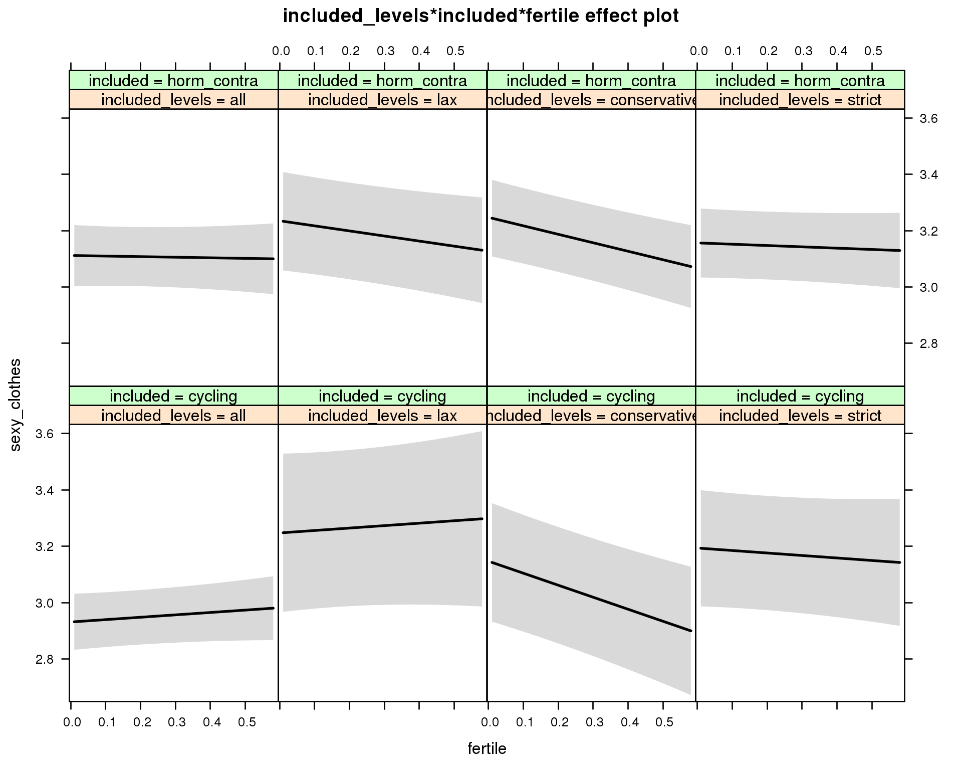
Linear mixed model fit by REML ['lmerMod']
Formula: sexy_clothes ~ menstruation + fertile_mean + (1 | person) + included_levels +
included + fertile + menstruation:included + included_levels:included +
included_levels:fertile + included:fertile + included_levels:included:fertile
Data: diary
REML criterion at convergence: 75849
Scaled residuals:
Min 1Q Median 3Q Max
-4.274 -0.610 -0.016 0.615 4.469
Random effects:
Groups Name Variance Std.Dev.
person (Intercept) 0.582 0.763
Residual 0.904 0.951
Number of obs: 26688, groups: person, 1054
Fixed effects:
Estimate Std. Error t value
(Intercept) 2.88010 0.07427 38.8
menstruationpre -0.09931 0.02904 -3.4
menstruationyes -0.14587 0.02734 -5.3
fertile_mean 0.54210 0.30978 1.7
included_levelslax 0.31609 0.15206 2.1
included_levelsconservative 0.21573 0.11867 1.8
included_levelsstrict 0.26259 0.11676 2.2
includedhorm_contra 0.15822 0.07667 2.1
fertile 0.08451 0.07400 1.1
menstruationpre:includedhorm_contra 0.03846 0.03729 1.0
menstruationyes:includedhorm_contra 0.08908 0.03588 2.5
included_levelslax:includedhorm_contra -0.19290 0.18511 -1.0
included_levelsconservative:includedhorm_contra -0.08040 0.14826 -0.5
included_levelsstrict:includedhorm_contra -0.21790 0.14353 -1.5
included_levelslax:fertile 0.00205 0.18074 0.0
included_levelsconservative:fertile -0.51083 0.13498 -3.8
included_levelsstrict:fertile -0.17304 0.13508 -1.3
includedhorm_contra:fertile -0.10491 0.11299 -0.9
included_levelslax:includedhorm_contra:fertile -0.16179 0.22051 -0.7
included_levelsconservative:includedhorm_contra:fertile 0.23029 0.17549 1.3
included_levelsstrict:includedhorm_contra:fertile 0.14677 0.17279 0.8
M_m6: Moderation by cycle length
model %>%
test_moderator("cycle_length_groups", diary, xlevels = 4)refitting model(s) with ML (instead of REML)
| Df | AIC | BIC | logLik | deviance | Chisq | Chi Df | Pr(>Chisq) | |
|---|---|---|---|---|---|---|---|---|
| with_main | 17 | 75835 | 75975 | -37901 | 75801 | NA | NA | NA |
| with_mod | 23 | 75828 | 76017 | -37891 | 75782 | 18.93 | 6 | 0.00429 |
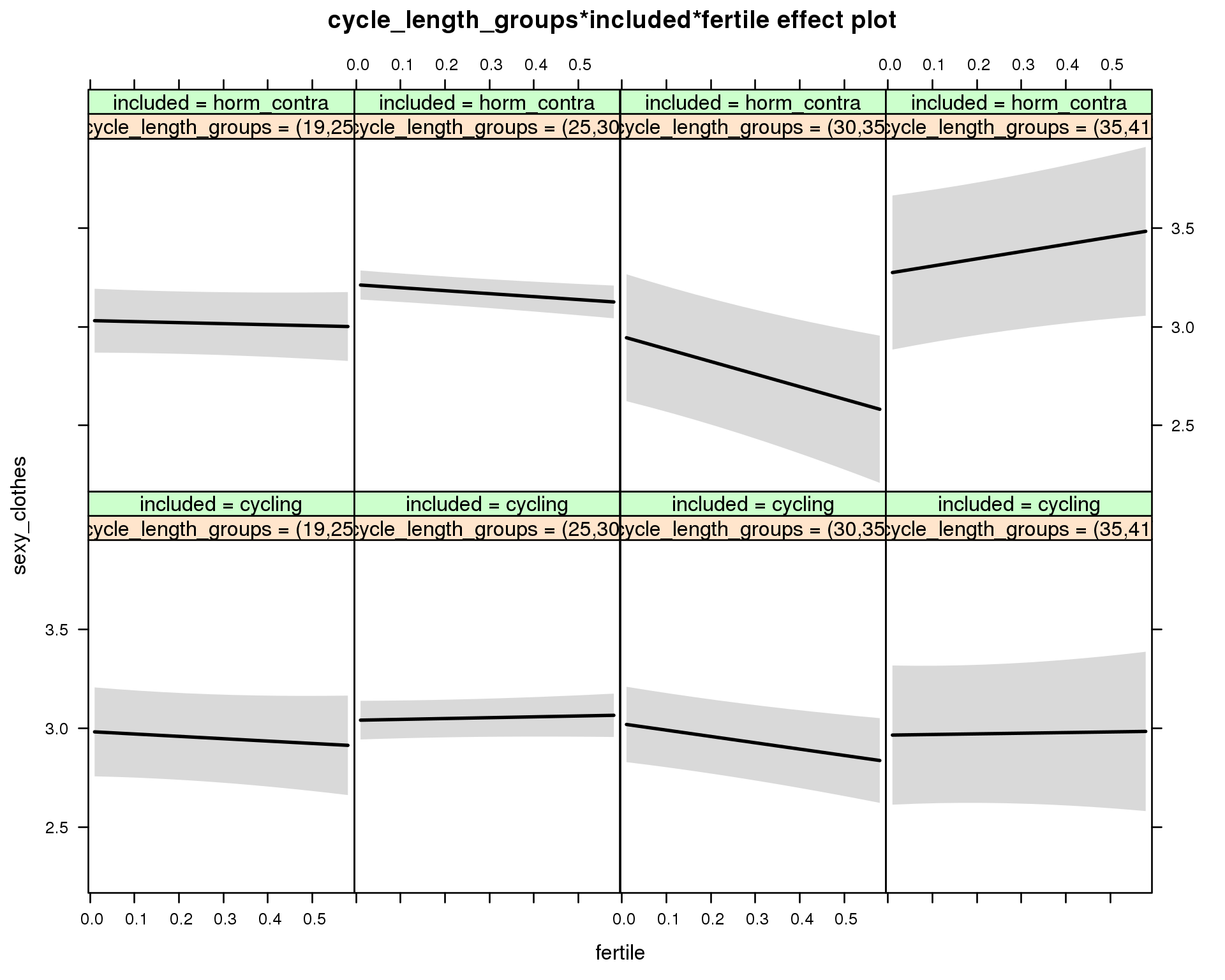
Linear mixed model fit by REML ['lmerMod']
Formula: sexy_clothes ~ menstruation + fertile_mean + (1 | person) + cycle_length_groups +
included + fertile + menstruation:included + cycle_length_groups:included +
cycle_length_groups:fertile + included:fertile + cycle_length_groups:included:fertile
Data: diary
REML criterion at convergence: 75846
Scaled residuals:
Min 1Q Median 3Q Max
-4.220 -0.610 -0.018 0.615 4.474
Random effects:
Groups Name Variance Std.Dev.
person (Intercept) 0.581 0.762
Residual 0.904 0.951
Number of obs: 26688, groups: person, 1054
Fixed effects:
Estimate Std. Error t value
(Intercept) 2.9254 0.1278 22.90
menstruationpre -0.0930 0.0291 -3.20
menstruationyes -0.1414 0.0275 -5.13
fertile_mean 0.5743 0.3108 1.85
cycle_length_groups(25,30] 0.0577 0.1255 0.46
cycle_length_groups(30,35] 0.0395 0.1509 0.26
cycle_length_groups(35,41] -0.0178 0.2138 -0.08
includedhorm_contra 0.0263 0.1426 0.18
fertile -0.1196 0.1545 -0.77
menstruationpre:includedhorm_contra 0.0338 0.0373 0.91
menstruationyes:includedhorm_contra 0.0856 0.0361 2.37
cycle_length_groups(25,30]:includedhorm_contra 0.1237 0.1548 0.80
cycle_length_groups(30,35]:includedhorm_contra -0.1200 0.2375 -0.51
cycle_length_groups(35,41]:includedhorm_contra 0.2574 0.3033 0.85
cycle_length_groups(25,30]:fertile 0.1626 0.1658 0.98
cycle_length_groups(30,35]:fertile -0.2005 0.1963 -1.02
cycle_length_groups(35,41]:fertile 0.1521 0.2773 0.55
includedhorm_contra:fertile 0.0679 0.1824 0.37
cycle_length_groups(25,30]:includedhorm_contra:fertile -0.2611 0.1964 -1.33
cycle_length_groups(30,35]:includedhorm_contra:fertile -0.3830 0.3091 -1.24
cycle_length_groups(35,41]:includedhorm_contra:fertile 0.2657 0.3651 0.73
M_m7: Moderation by certainty about menstruation parameters
model %>%
test_moderator("certainty_menstruation", diary)refitting model(s) with ML (instead of REML)
| Df | AIC | BIC | logLik | deviance | Chisq | Chi Df | Pr(>Chisq) | |
|---|---|---|---|---|---|---|---|---|
| with_main | 13 | 75835 | 75941 | -37904 | 75809 | NA | NA | NA |
| with_mod | 15 | 75835 | 75958 | -37903 | 75805 | 3.334 | 2 | 0.1888 |
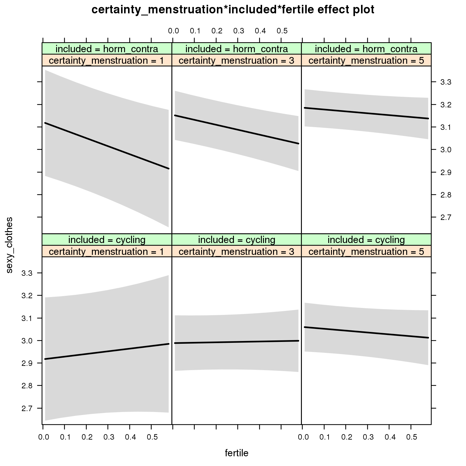
Linear mixed model fit by REML ['lmerMod']
Formula: sexy_clothes ~ menstruation + fertile_mean + (1 | person) + certainty_menstruation +
included + fertile + menstruation:included + certainty_menstruation:included +
certainty_menstruation:fertile + included:fertile + certainty_menstruation:included:fertile
Data: diary
REML criterion at convergence: 75864
Scaled residuals:
Min 1Q Median 3Q Max
-4.216 -0.607 -0.019 0.617 4.484
Random effects:
Groups Name Variance Std.Dev.
person (Intercept) 0.583 0.764
Residual 0.904 0.951
Number of obs: 26688, groups: person, 1054
Fixed effects:
Estimate Std. Error t value
(Intercept) 2.8198 0.1880 15.00
menstruationpre -0.0956 0.0290 -3.29
menstruationyes -0.1446 0.0274 -5.28
fertile_mean 0.5939 0.3079 1.93
certainty_menstruation 0.0359 0.0428 0.84
includedhorm_contra 0.2022 0.2386 0.85
fertile 0.1681 0.2305 0.73
menstruationpre:includedhorm_contra 0.0369 0.0373 0.99
menstruationyes:includedhorm_contra 0.0914 0.0359 2.55
certainty_menstruation:includedhorm_contra -0.0198 0.0556 -0.36
certainty_menstruation:fertile -0.0501 0.0540 -0.93
includedhorm_contra:fertile -0.5920 0.2996 -1.98
certainty_menstruation:includedhorm_contra:fertile 0.1182 0.0692 1.71
M_m8: Moderation by cycle regularity
model %>%
test_moderator("cycle_regularity", diary)refitting model(s) with ML (instead of REML)
| Df | AIC | BIC | logLik | deviance | Chisq | Chi Df | Pr(>Chisq) | |
|---|---|---|---|---|---|---|---|---|
| with_main | 15 | 75834 | 75957 | -37902 | 75804 | NA | NA | NA |
| with_mod | 19 | 75834 | 75989 | -37898 | 75796 | 8.432 | 4 | 0.07698 |
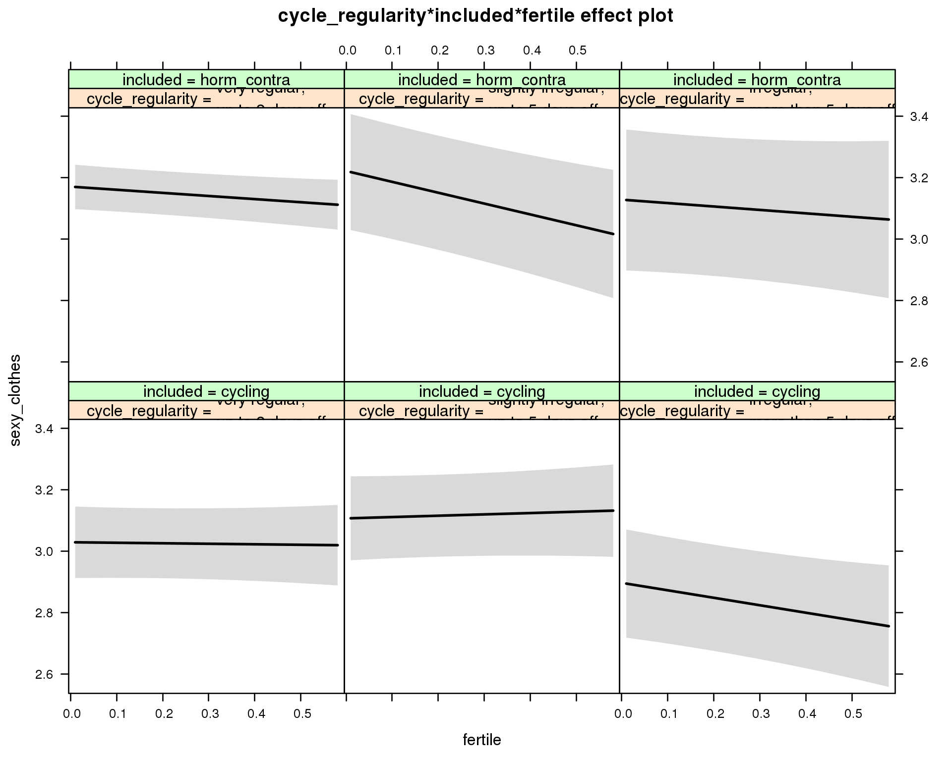
Linear mixed model fit by REML ['lmerMod']
Formula: sexy_clothes ~ menstruation + fertile_mean + (1 | person) + cycle_regularity +
included + fertile + menstruation:included + cycle_regularity:included +
cycle_regularity:fertile + included:fertile + cycle_regularity:included:fertile
Data: diary
REML criterion at convergence: 75857
Scaled residuals:
Min 1Q Median 3Q Max
-4.239 -0.608 -0.020 0.616 4.492
Random effects:
Groups Name Variance Std.Dev.
person (Intercept) 0.582 0.763
Residual 0.904 0.951
Number of obs: 26688, groups: person, 1054
Fixed effects:
Estimate Std. Error t value
(Intercept) 2.9713 0.0790 37.6
menstruationpre -0.0933 0.0290 -3.2
menstruationyes -0.1418 0.0274 -5.2
fertile_mean 0.5693 0.3086 1.8
cycle_regularityslightly irregular,\nup to 5 days off 0.0777 0.0915 0.8
cycle_regularityirregular,\nmore than 5 days off -0.1322 0.1076 -1.2
includedhorm_contra 0.1209 0.0719 1.7
fertile -0.0165 0.0811 -0.2
menstruationpre:includedhorm_contra 0.0340 0.0373 0.9
menstruationyes:includedhorm_contra 0.0874 0.0359 2.4
cycle_regularityslightly irregular,\nup to 5 days off:includedhorm_contra -0.0268 0.1381 -0.2
cycle_regularityirregular,\nmore than 5 days off:includedhorm_contra 0.0898 0.1634 0.5
cycle_regularityslightly irregular,\nup to 5 days off:fertile 0.0599 0.1119 0.5
cycle_regularityirregular,\nmore than 5 days off:fertile -0.2267 0.1375 -1.6
includedhorm_contra:fertile -0.0850 0.0950 -0.9
cycle_regularityslightly irregular,\nup to 5 days off:includedhorm_contra:fertile -0.3119 0.1661 -1.9
cycle_regularityirregular,\nmore than 5 days off:includedhorm_contra:fertile 0.2168 0.2051 1.1
M_m9: Moderation by cohabitation status
model %>%
test_moderator("cohabitation", diary)refitting model(s) with ML (instead of REML)
| Df | AIC | BIC | logLik | deviance | Chisq | Chi Df | Pr(>Chisq) | |
|---|---|---|---|---|---|---|---|---|
| with_main | 15 | 75827 | 75949 | -37898 | 75797 | NA | NA | NA |
| with_mod | 19 | 75830 | 75985 | -37896 | 75792 | 4.785 | 4 | 0.3101 |
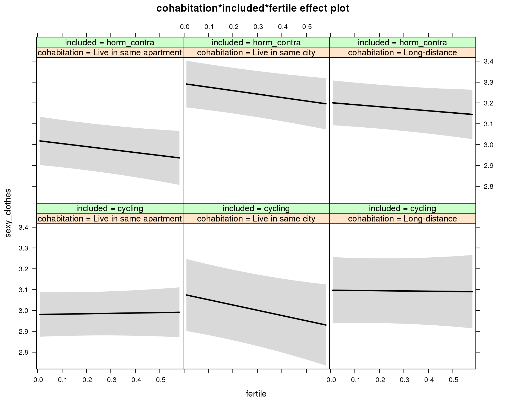
Linear mixed model fit by REML ['lmerMod']
Formula: sexy_clothes ~ menstruation + fertile_mean + (1 | person) + cohabitation +
included + fertile + menstruation:included + cohabitation:included +
cohabitation:fertile + included:fertile + cohabitation:included:fertile
Data: diary
REML criterion at convergence: 75856
Scaled residuals:
Min 1Q Median 3Q Max
-4.216 -0.608 -0.018 0.618 4.557
Random effects:
Groups Name Variance Std.Dev.
person (Intercept) 0.578 0.760
Residual 0.904 0.951
Number of obs: 26688, groups: person, 1054
Fixed effects:
Estimate Std. Error t value
(Intercept) 2.9197 0.0763 38.3
menstruationpre -0.0952 0.0290 -3.3
menstruationyes -0.1441 0.0273 -5.3
fertile_mean 0.5947 0.3069 1.9
cohabitationLive in same city 0.0962 0.1035 0.9
cohabitationLong-distance 0.1165 0.0976 1.2
includedhorm_contra 0.0160 0.0819 0.2
fertile 0.0186 0.0732 0.3
menstruationpre:includedhorm_contra 0.0352 0.0373 0.9
menstruationyes:includedhorm_contra 0.0885 0.0358 2.5
cohabitationLive in same city:includedhorm_contra 0.1770 0.1323 1.3
cohabitationLong-distance:includedhorm_contra 0.0657 0.1266 0.5
cohabitationLive in same city:fertile -0.2711 0.1338 -2.0
cohabitationLong-distance:fertile -0.0304 0.1205 -0.3
includedhorm_contra:fertile -0.1612 0.1070 -1.5
cohabitationLive in same city:includedhorm_contra:fertile 0.2477 0.1672 1.5
cohabitationLong-distance:includedhorm_contra:fertile 0.0757 0.1552 0.5
M_m10: Moderation by relationship status
model %>%
test_moderator("relationship_status_clean", diary)refitting model(s) with ML (instead of REML)
| Df | AIC | BIC | logLik | deviance | Chisq | Chi Df | Pr(>Chisq) | |
|---|---|---|---|---|---|---|---|---|
| with_main | 15 | 75828 | 75950 | -37899 | 75798 | NA | NA | NA |
| with_mod | 19 | 75828 | 75983 | -37895 | 75790 | 7.972 | 4 | 0.09262 |

Linear mixed model fit by REML ['lmerMod']
Formula: sexy_clothes ~ menstruation + fertile_mean + (1 | person) + relationship_status_clean +
included + fertile + menstruation:included + relationship_status_clean:included +
relationship_status_clean:fertile + included:fertile + relationship_status_clean:included:fertile
Data: diary
REML criterion at convergence: 75845
Scaled residuals:
Min 1Q Median 3Q Max
-4.226 -0.607 -0.018 0.617 4.510
Random effects:
Groups Name Variance Std.Dev.
person (Intercept) 0.578 0.760
Residual 0.904 0.951
Number of obs: 26688, groups: person, 1054
Fixed effects:
Estimate Std. Error t value
(Intercept) 2.9870 0.0714 41.8
menstruationpre -0.0954 0.0290 -3.3
menstruationyes -0.1432 0.0273 -5.2
fertile_mean 0.5985 0.3066 2.0
relationship_status_cleanVerheiratet -0.1169 0.0946 -1.2
relationship_status_cleanVerlobt 0.1532 0.1824 0.8
includedhorm_contra 0.1275 0.0612 2.1
fertile -0.0864 0.0671 -1.3
menstruationpre:includedhorm_contra 0.0360 0.0373 1.0
menstruationyes:includedhorm_contra 0.0886 0.0358 2.5
relationship_status_cleanVerheiratet:includedhorm_contra -0.3704 0.1823 -2.0
relationship_status_cleanVerlobt:includedhorm_contra -0.2118 0.2692 -0.8
relationship_status_cleanVerheiratet:fertile 0.2567 0.1181 2.2
relationship_status_cleanVerlobt:fertile -0.2691 0.2214 -1.2
includedhorm_contra:fertile -0.0453 0.0817 -0.6
relationship_status_cleanVerheiratet:includedhorm_contra:fertile -0.3650 0.2223 -1.6
relationship_status_cleanVerlobt:includedhorm_contra:fertile 0.4643 0.3438 1.4
Showy clothes
model_summaries$showy_clothesModel summary
Model summary
model %>%
print_summary()Linear mixed model fit by REML
t-tests use Satterthwaite approximations to degrees of freedom ['lmerMod']
Formula: showy_clothes ~ included * (menstruation + fertile) + fertile_mean + (1 | person)
Data: diary
REML criterion at convergence: 84664
Scaled residuals:
Min 1Q Median 3Q Max
-3.717 -0.629 -0.104 0.622 4.118
Random effects:
Groups Name Variance Std.Dev.
person (Intercept) 0.811 0.90
Residual 1.259 1.12
Number of obs: 26685, groups: person, 1054
Fixed effects:
Estimate Std. Error df t value Pr(>|t|)
(Intercept) 2.6074 0.0790 1430.0000 33.02 < 2e-16 ***
includedhorm_contra 0.0569 0.0647 1392.0000 0.88 0.37906
menstruationpre -0.0689 0.0342 26014.0000 -2.01 0.04427 *
menstruationyes -0.1134 0.0323 26122.0000 -3.51 0.00044 ***
fertile -0.0604 0.0691 25998.0000 -0.87 0.38173
fertile_mean 0.6089 0.3624 1552.0000 1.68 0.09313 .
includedhorm_contra:menstruationpre 0.0370 0.0440 26011.0000 0.84 0.40001
includedhorm_contra:menstruationyes 0.0671 0.0423 26099.0000 1.59 0.11243
includedhorm_contra:fertile -0.0834 0.0875 26123.0000 -0.95 0.34054
---
Signif. codes: 0 '***' 0.001 '**' 0.01 '*' 0.05 '.' 0.1 ' ' 1
Correlation of Fixed Effects:
(Intr) incld_ mnstrtnp mnstrtny fertil frtl_m inclddhrm_cntr:mnstrtnp
inclddhrm_c -0.473
menstrutnpr -0.167 0.212
menstrutnys -0.163 0.204 0.397
fertile -0.160 0.262 0.467 0.384
fertile_men -0.772 -0.026 -0.008 -0.005 -0.068
inclddhrm_cntr:mnstrtnp 0.138 -0.265 -0.779 -0.309 -0.363 -0.004
inclddhrm_cntr:mnstrtny 0.130 -0.250 -0.303 -0.763 -0.293 -0.004 0.383
inclddhrm_cntr:f 0.160 -0.331 -0.368 -0.303 -0.786 0.010 0.466
inclddhrm_cntr:mnstrtny
inclddhrm_c
menstrutnpr
menstrutnys
fertile
fertile_men
inclddhrm_cntr:mnstrtnp
inclddhrm_cntr:mnstrtny
inclddhrm_cntr:f 0.381
Effect size standardised by residual variance (\(\frac{b}{ SD_{residual} }\)): -0.05 [-0.17;0.07].
Marginal effect plots
model %>%
plot_all_effects()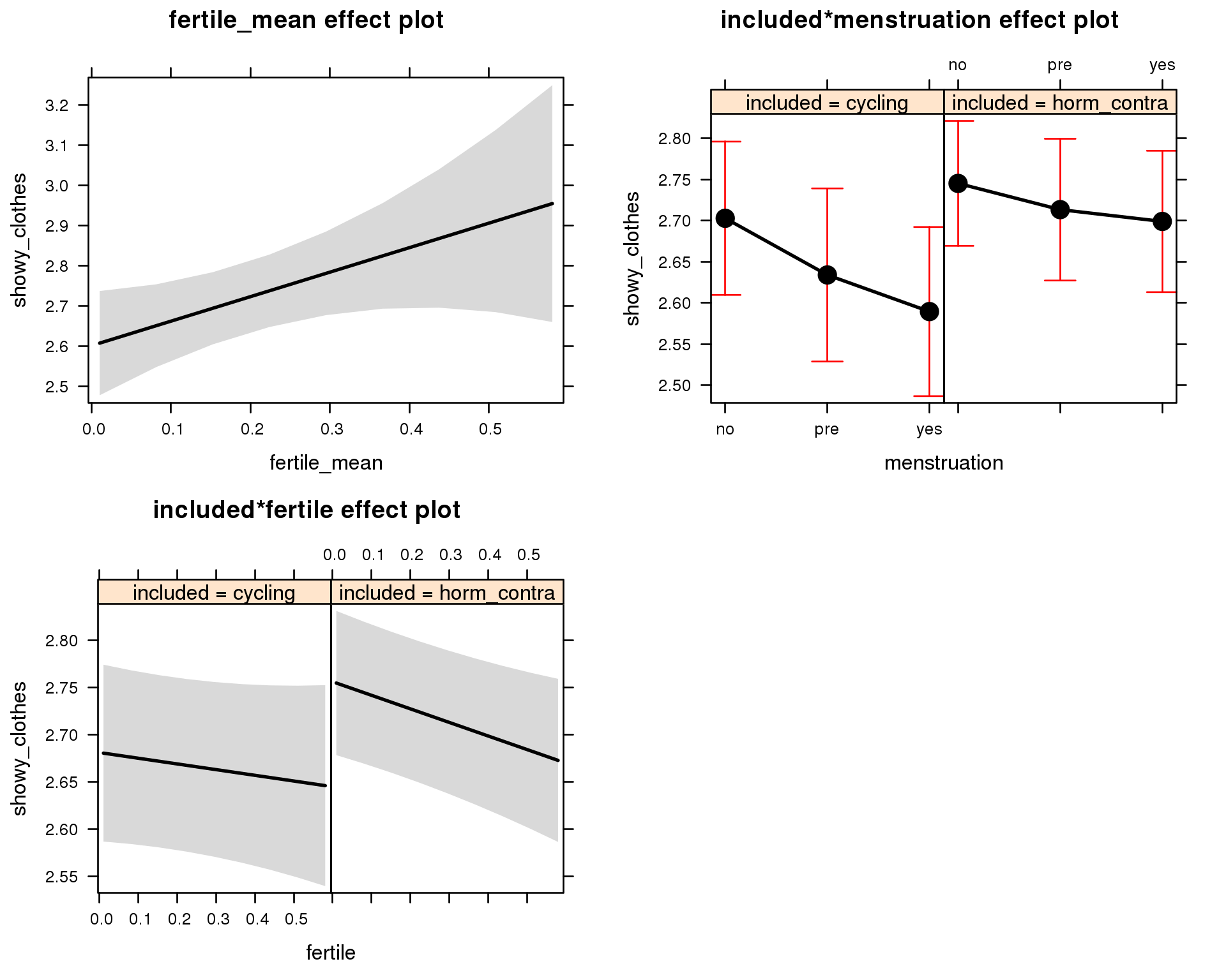
Outcome distribution
model %>%
plot_outcome(diary) + xlab(outcome_label)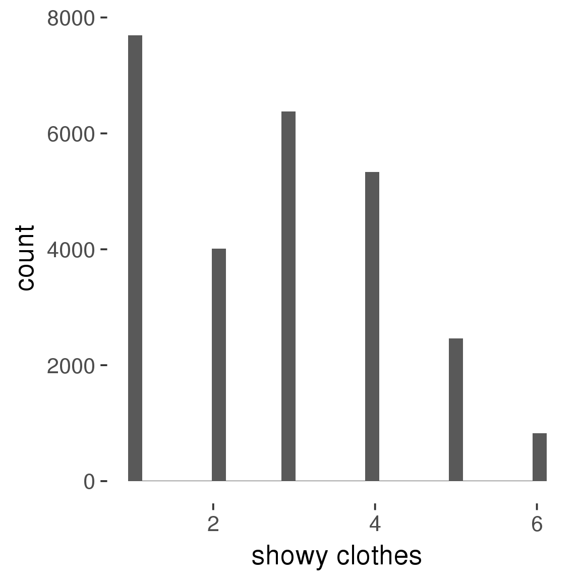
Diagnostics
model %>%
print_diagnostics()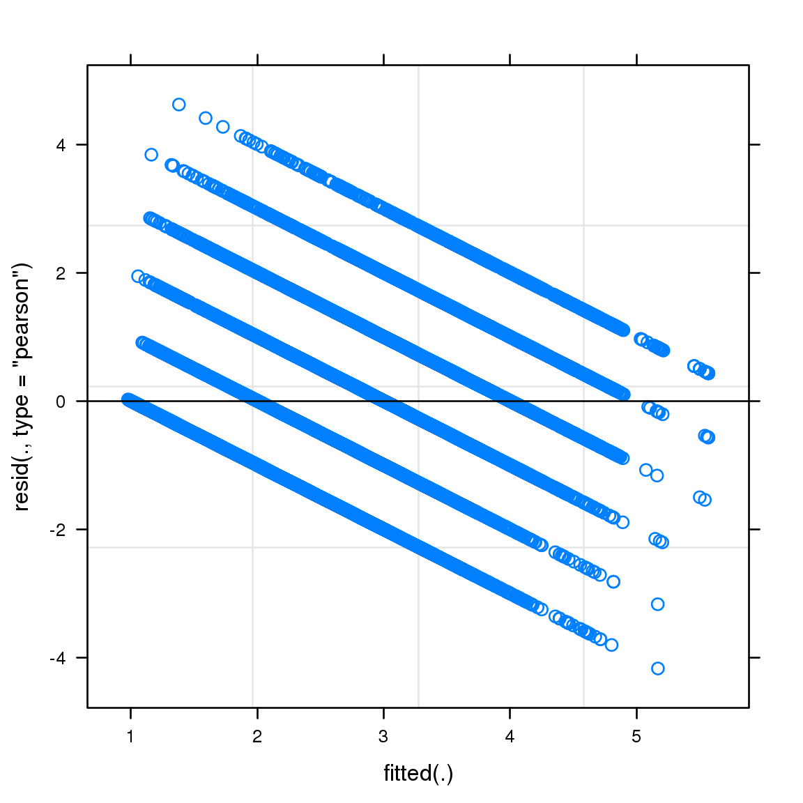
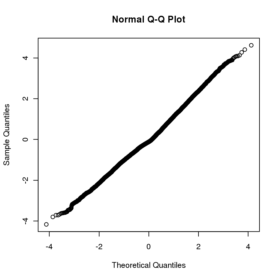

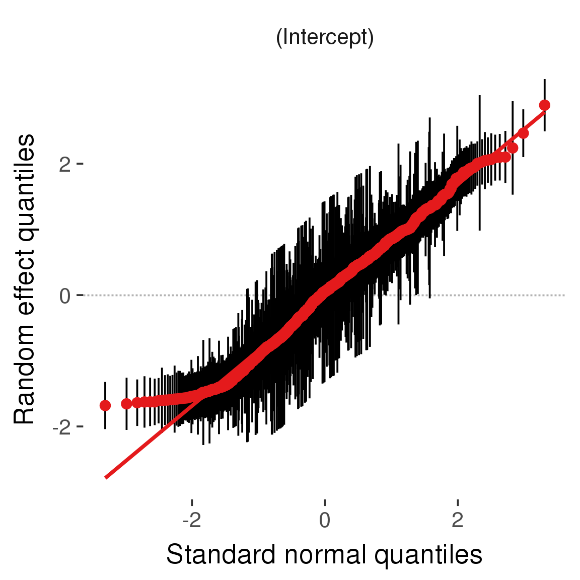
Curves
Here, we continuously plot the outcome over the course of the cycle. Because cycle lengths vary, we subset the data to cycles in a certain range. If the red curve traces the pink curve, our predictor accurately maps the relationship between fertile window probability and the outcome.
Cycle lengths from 21 to 36
Backward-counted
model %>%
plot_curve(diary %>% filter(minimum_cycle_length_diary <= 36, minimum_cycle_length_diary > 20) %>% mutate(fertile=prc_stirn_b))outcome = names(model@frame)[1]
outcome_label = recode(str_replace_all(str_replace_all(str_replace_all(outcome, "_", " "), " pair", "-pair"), " 1", ""),
"desirability 1" = "self-perceived desirability",
"NARQ admiration" = "narcissistic admiration",
"NARQ rivalry" = "narcissistic rivalry",
"extra-pair" = "extra-pair desire & behaviour",
"had sexual intercourse" = "sexual intercourse")
library(ggplot2)
# form a subset and run the model without the hormonal contraception and the fertility predictors
tmp = diary %>%
filter(!is.na(fertile), !is.na(included),
RCD > -1 * minimum_cycle_length_diary, RCD > -40)
new_form = update.formula(formula(model), new = . ~ . - fertile * included)
tmp$residuals = residuals(update(model, new_form, data = tmp , na.action = na.exclude))
tmp = tmp %>%
filter(!is.na(RCD), !is.na(residuals))
rcd_min = min(tmp$RCD)
tmp$real = FALSE
tmp_before = tmp
tmp_before$RCD = tmp_before$RCD + min(tmp$RCD) - 1
tmp_after = tmp
tmp_after$RCD = tmp_after$RCD - min(tmp$RCD) + 1
tmp$real = TRUE
tmp = bind_rows(tmp_before %>% filter(RCD > rcd_min - 11), tmp, tmp_after %>% filter(RCD < 11))GAM smooth on residuals
Here, we partialled out menstruation and individual random effects, then superimposed estimated probability of being in the fertile window scaled to the range of the estimated means. To address the periodicity of the cycle, we prepended and appended ten days of the timeseries to the end and the beginning of the timeseries. We then estimated the GAM and cut off the appended subsets before plotting.
tryCatch({
trend_plot = ggplot(tmp,aes(x = RCD, y = residuals, colour = included)) +
stat_smooth(geom = 'smooth',size = 0.8, fill = "#9ECAE1", method = 'gam', formula = y ~ s(x))
}, error = function(e){cat_message(e, "danger")})
tryCatch({
trend_data = ggplot_build(trend_plot)$data[[1]]
}, error = function(e){cat_message(e, "danger")})
trend_data$RCD = round(trend_data$x)
trend_data = left_join(trend_data, tmp %>% select(real, RCD,fertile) %>% unique(), by = "RCD")
trend_data %>%
filter(real == TRUE) %>%
mutate(superimposed = ( ( (fertile - 0.01)/0.58) * (max(y)-min(y) ) ) + min(y) ) ->
trend_data
ggplot(trend_data) +
geom_ribbon(aes(x = x, ymin = ymin, ymax = ymax, fill = factor(group)), alpha = 0.2) +
geom_line(aes(x = x, y = y, colour = factor(group)), size = 0.8, stat = "identity") +
scale_x_continuous(caption_x) +
geom_line(aes(x = x, y = superimposed), color = "#a83fbf", size = 1, linetype = 'dashed') +
annotate("text",x = mean(trend_data$x), y = max(trend_data$superimposed,na.rm=T) + 0.1, label = 'superimposed fertility peak', color = "#a83fbf") +
scale_y_continuous(outcome_label) +
ggtitle("GAM smooth, residuals") +
scale_color_manual("Contraception status",values = c("2"="black","1"= "red"), labels = c("2"="hormonally\ncontracepting","1"="cycling"), guide = F) +
scale_fill_manual("Contraception status",values = c("2"="black","1"= "red"), labels = c("2"="hormonally\ncontracepting","1"="cycling"), guide = F)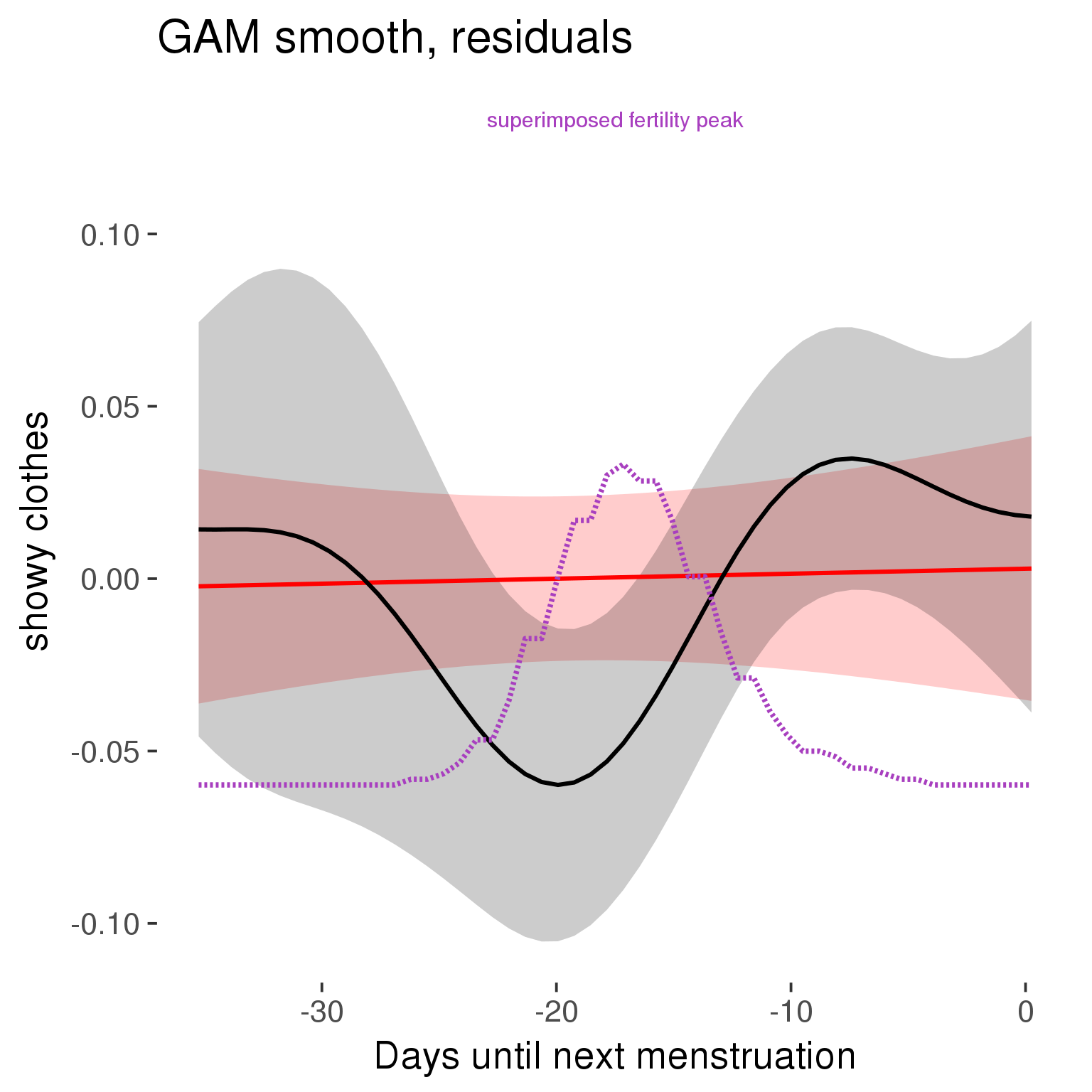
GAM smooth on raw data
As before, but without partialling anything out.
tryCatch({
trend_plot = ggplot(tmp,aes_string(x = "RCD", y = outcome, colour = "included")) +
stat_smooth(geom = 'smooth',size = 0.8, fill = "#9ECAE1", method = 'gam', formula = y ~ s(x))
}, error = function(e){cat_message(e, "danger")})
tryCatch({
trend_data = ggplot_build(trend_plot)$data[[1]]
}, error = function(e){cat_message(e, "danger")})
trend_data$RCD = round(trend_data$x)
trend_data = left_join(trend_data, tmp %>% select(real, RCD,fertile) %>% unique(), by = "RCD")
trend_data %>%
filter(real == TRUE) %>%
mutate(superimposed = ( ( (fertile - 0.01)/0.58) * (max(y)-min(y) ) ) + min(y) ) ->
trend_data
plot1b = ggplot(trend_data) +
geom_ribbon(aes(x = x, ymin = ymin, ymax = ymax, fill = factor(group)), alpha = 0.2) +
geom_line(aes(x = x, y = y, colour = factor(group)), size = 0.8, stat = "identity") +
scale_x_continuous(caption_x) +
geom_line(aes(x = x, y = superimposed), color = "#a83fbf", size = 1, linetype = 'dashed') +
annotate("text",x = mean(trend_data$x), y = max(trend_data$superimposed,na.rm=T) + 0.1, label = 'superimposed fertility peak', color = "#a83fbf") +
scale_y_continuous(outcome_label) +
ggtitle("GAM smooth, raw data") +
scale_color_manual("Contraception status",values = c("2"="black","1"= "red"), labels = c("2"="hormonally\ncontracepting","1"="cycling"), guide = F) +
scale_fill_manual("Contraception status",values = c("2"="black","1"= "red"), labels = c("2"="hormonally\ncontracepting","1"="cycling"), guide = F)
suppressWarnings(print(plot1b))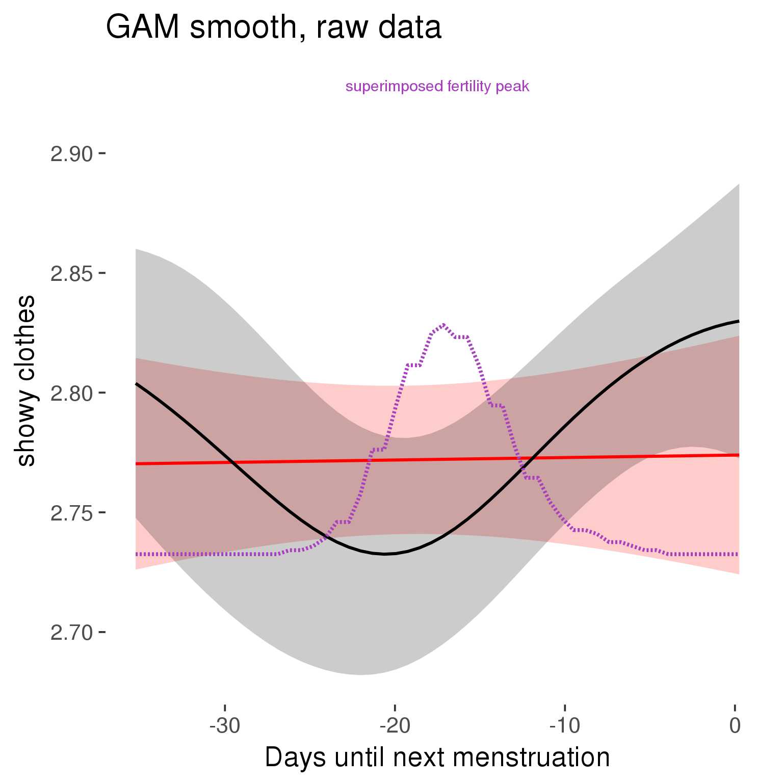
Means and standard errors over raw data
Nothing partialled out, just straight means with bootstrapped confidence intervals.
tryCatch({
trend_plot = ggplot(tmp,aes_string(x = "RCD", y = outcome, colour = "included")) +
geom_pointrange(size = 0.8, stat = 'summary', fun.data = "mean_cl_boot")
}, error = function(e){cat_message(e, "danger")})
tryCatch({
trend_data = ggplot_build(trend_plot)$data[[1]]
}, error = function(e){cat_message(e, "danger")})
trend_data$RCD = round(trend_data$x)
trend_data = left_join(trend_data, tmp %>% select(real, RCD,fertile) %>% unique(), by = "RCD")
trend_data %>%
filter(real == TRUE) %>%
mutate(superimposed = ( ( (fertile - 0.01)/0.58) * (max(y)-min(y) ) ) + min(y) ) ->
trend_data
plot3 = ggplot(trend_data) +
geom_pointrange(aes(x = x, y = y, ymin = ymin,ymax = ymax, colour = factor(group)), size = 0.8, stat = "identity", alpha = 0.6, position = position_dodge(width = .5)) +
scale_x_continuous("Days until next menstruation") +
geom_line(aes(x= x, y = superimposed), color = "#a83fbf", size = 1, linetype = 'dashed') +
annotate("text",x = mean(trend_data$x), y = max(trend_data$superimposed,na.rm=T) + 0.1, label = 'superimposed fertility peak', color = "#a83fbf") +
scale_y_continuous(outcome_label) +
ggtitle("Means with standard errors, raw data") +
scale_color_manual("Contraception status",values = c("2"="black","1"= "red"), labels = c("2"="hormonally\ncontracepting","1"="cycling"), guide = F) +
scale_fill_manual("Contraception status",values = c("2"="black","1"= "red"), labels = c("2"="hormonally\ncontracepting","1"="cycling"), guide = F)
suppressWarnings(print(plot3))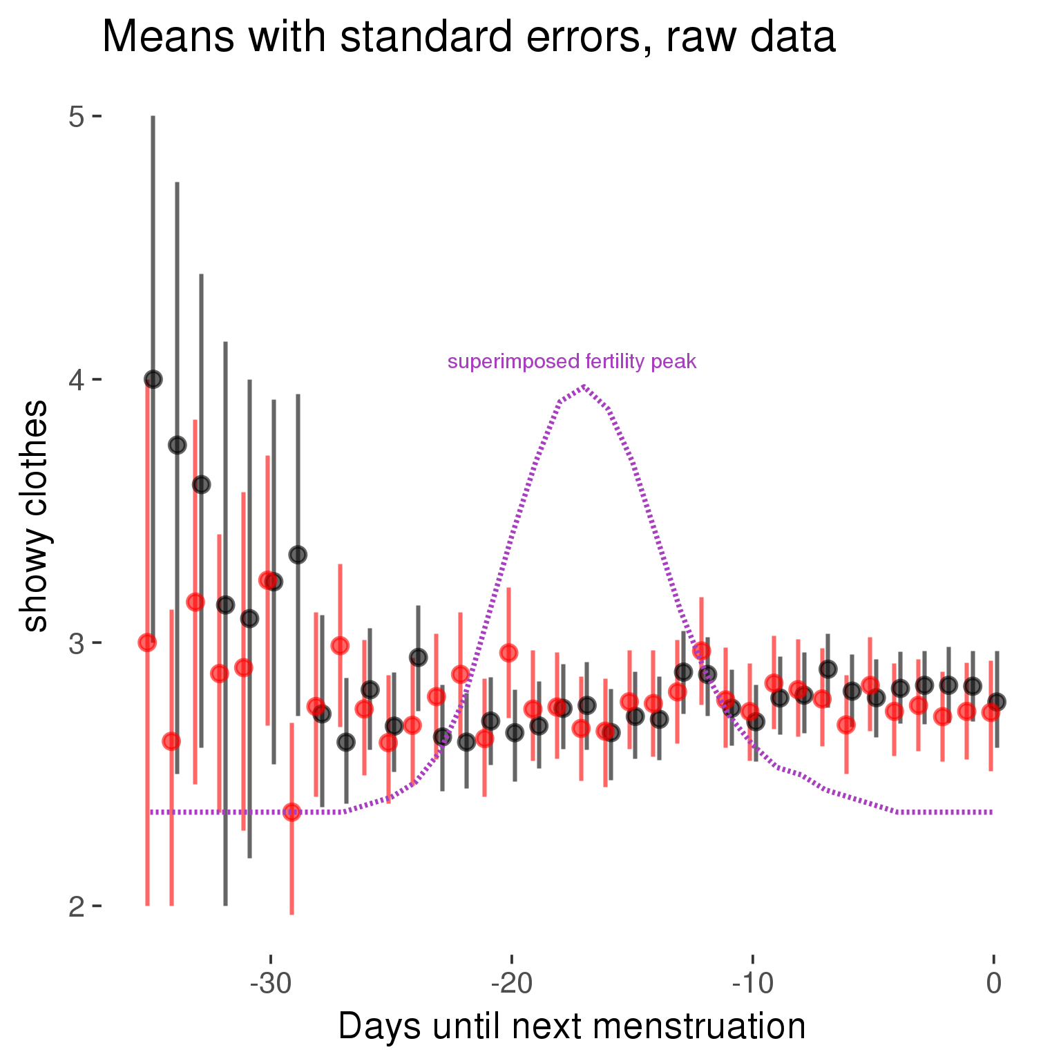
Forward-counted
model %>%
plot_curve(diary %>% filter(minimum_cycle_length_diary <= 36, minimum_cycle_length_diary > 20) %>% mutate(RCD = FCD, fertile = prc_stirn_b_forward_counted), caption_x = "Days since last menstruation")outcome = names(model@frame)[1]
outcome_label = recode(str_replace_all(str_replace_all(str_replace_all(outcome, "_", " "), " pair", "-pair"), " 1", ""),
"desirability 1" = "self-perceived desirability",
"NARQ admiration" = "narcissistic admiration",
"NARQ rivalry" = "narcissistic rivalry",
"extra-pair" = "extra-pair desire & behaviour",
"had sexual intercourse" = "sexual intercourse")
library(ggplot2)
# form a subset and run the model without the hormonal contraception and the fertility predictors
tmp = diary %>%
filter(!is.na(fertile), !is.na(included),
RCD > -1 * minimum_cycle_length_diary, RCD > -40)
new_form = update.formula(formula(model), new = . ~ . - fertile * included)
tmp$residuals = residuals(update(model, new_form, data = tmp , na.action = na.exclude))
tmp = tmp %>%
filter(!is.na(RCD), !is.na(residuals))
rcd_min = min(tmp$RCD)
tmp$real = FALSE
tmp_before = tmp
tmp_before$RCD = tmp_before$RCD + min(tmp$RCD) - 1
tmp_after = tmp
tmp_after$RCD = tmp_after$RCD - min(tmp$RCD) + 1
tmp$real = TRUE
tmp = bind_rows(tmp_before %>% filter(RCD > rcd_min - 11), tmp, tmp_after %>% filter(RCD < 11))GAM smooth on residuals
Here, we partialled out menstruation and individual random effects, then superimposed estimated probability of being in the fertile window scaled to the range of the estimated means. To address the periodicity of the cycle, we prepended and appended ten days of the timeseries to the end and the beginning of the timeseries. We then estimated the GAM and cut off the appended subsets before plotting.
tryCatch({
trend_plot = ggplot(tmp,aes(x = RCD, y = residuals, colour = included)) +
stat_smooth(geom = 'smooth',size = 0.8, fill = "#9ECAE1", method = 'gam', formula = y ~ s(x))
}, error = function(e){cat_message(e, "danger")})
tryCatch({
trend_data = ggplot_build(trend_plot)$data[[1]]
}, error = function(e){cat_message(e, "danger")})
trend_data$RCD = round(trend_data$x)
trend_data = left_join(trend_data, tmp %>% select(real, RCD,fertile) %>% unique(), by = "RCD")
trend_data %>%
filter(real == TRUE) %>%
mutate(superimposed = ( ( (fertile - 0.01)/0.58) * (max(y)-min(y) ) ) + min(y) ) ->
trend_data
ggplot(trend_data) +
geom_ribbon(aes(x = x, ymin = ymin, ymax = ymax, fill = factor(group)), alpha = 0.2) +
geom_line(aes(x = x, y = y, colour = factor(group)), size = 0.8, stat = "identity") +
scale_x_continuous(caption_x) +
geom_line(aes(x = x, y = superimposed), color = "#a83fbf", size = 1, linetype = 'dashed') +
annotate("text",x = mean(trend_data$x), y = max(trend_data$superimposed,na.rm=T) + 0.1, label = 'superimposed fertility peak', color = "#a83fbf") +
scale_y_continuous(outcome_label) +
ggtitle("GAM smooth, residuals") +
scale_color_manual("Contraception status",values = c("2"="black","1"= "red"), labels = c("2"="hormonally\ncontracepting","1"="cycling"), guide = F) +
scale_fill_manual("Contraception status",values = c("2"="black","1"= "red"), labels = c("2"="hormonally\ncontracepting","1"="cycling"), guide = F)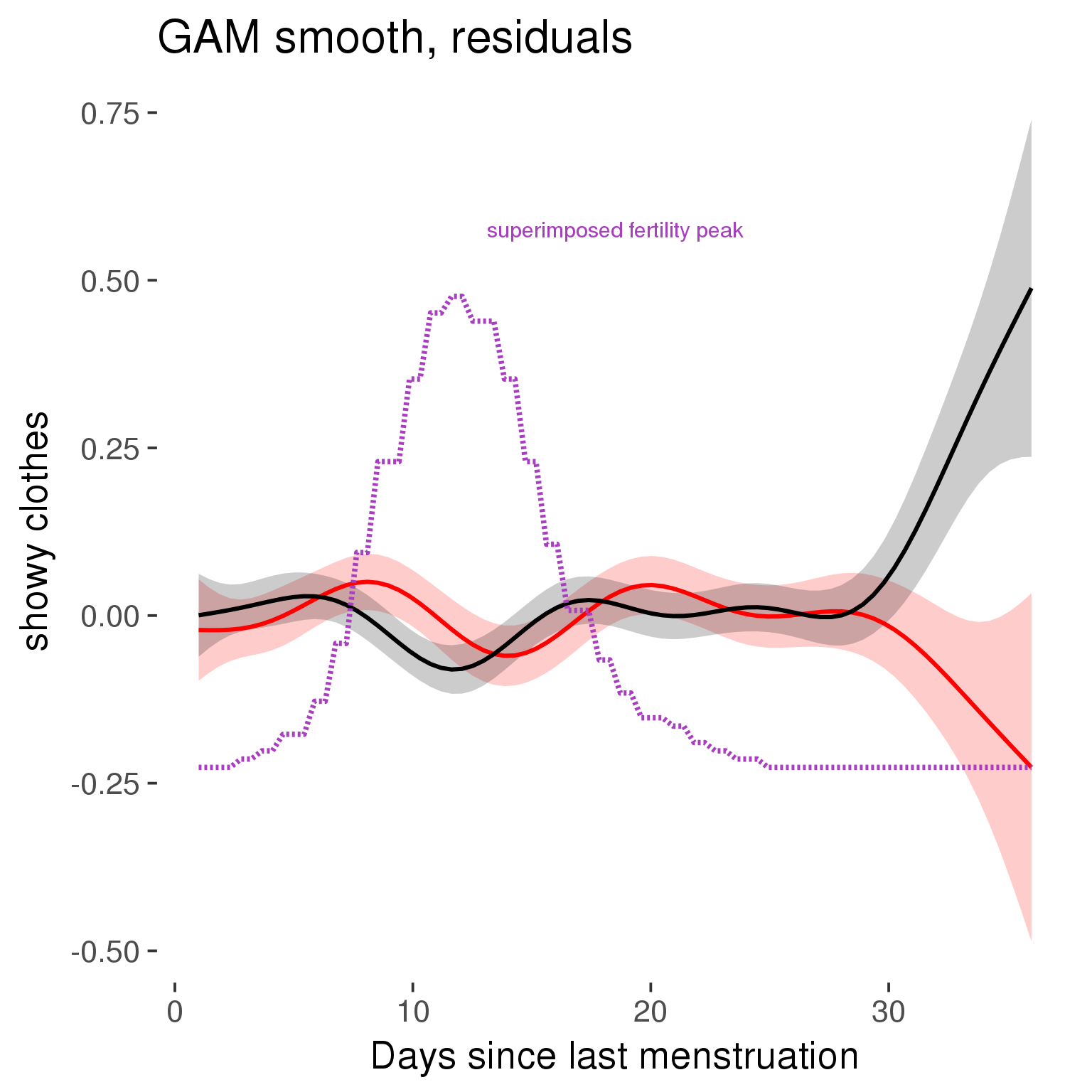
GAM smooth on raw data
As before, but without partialling anything out.
tryCatch({
trend_plot = ggplot(tmp,aes_string(x = "RCD", y = outcome, colour = "included")) +
stat_smooth(geom = 'smooth',size = 0.8, fill = "#9ECAE1", method = 'gam', formula = y ~ s(x))
}, error = function(e){cat_message(e, "danger")})
tryCatch({
trend_data = ggplot_build(trend_plot)$data[[1]]
}, error = function(e){cat_message(e, "danger")})
trend_data$RCD = round(trend_data$x)
trend_data = left_join(trend_data, tmp %>% select(real, RCD,fertile) %>% unique(), by = "RCD")
trend_data %>%
filter(real == TRUE) %>%
mutate(superimposed = ( ( (fertile - 0.01)/0.58) * (max(y)-min(y) ) ) + min(y) ) ->
trend_data
plot1b = ggplot(trend_data) +
geom_ribbon(aes(x = x, ymin = ymin, ymax = ymax, fill = factor(group)), alpha = 0.2) +
geom_line(aes(x = x, y = y, colour = factor(group)), size = 0.8, stat = "identity") +
scale_x_continuous(caption_x) +
geom_line(aes(x = x, y = superimposed), color = "#a83fbf", size = 1, linetype = 'dashed') +
annotate("text",x = mean(trend_data$x), y = max(trend_data$superimposed,na.rm=T) + 0.1, label = 'superimposed fertility peak', color = "#a83fbf") +
scale_y_continuous(outcome_label) +
ggtitle("GAM smooth, raw data") +
scale_color_manual("Contraception status",values = c("2"="black","1"= "red"), labels = c("2"="hormonally\ncontracepting","1"="cycling"), guide = F) +
scale_fill_manual("Contraception status",values = c("2"="black","1"= "red"), labels = c("2"="hormonally\ncontracepting","1"="cycling"), guide = F)
suppressWarnings(print(plot1b))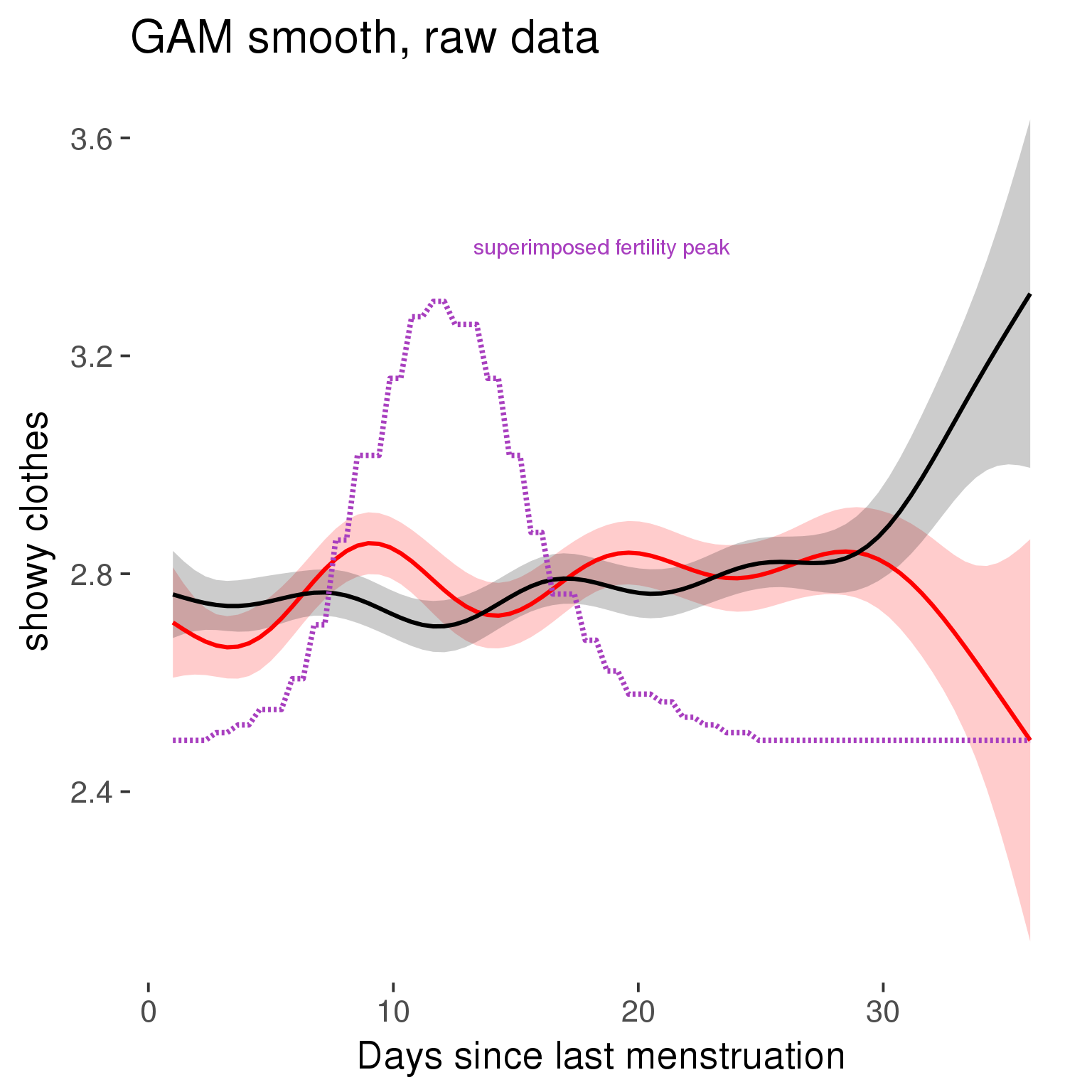
Means and standard errors over raw data
Nothing partialled out, just straight means with bootstrapped confidence intervals.
tryCatch({
trend_plot = ggplot(tmp,aes_string(x = "RCD", y = outcome, colour = "included")) +
geom_pointrange(size = 0.8, stat = 'summary', fun.data = "mean_cl_boot")
}, error = function(e){cat_message(e, "danger")})
tryCatch({
trend_data = ggplot_build(trend_plot)$data[[1]]
}, error = function(e){cat_message(e, "danger")})
trend_data$RCD = round(trend_data$x)
trend_data = left_join(trend_data, tmp %>% select(real, RCD,fertile) %>% unique(), by = "RCD")
trend_data %>%
filter(real == TRUE) %>%
mutate(superimposed = ( ( (fertile - 0.01)/0.58) * (max(y)-min(y) ) ) + min(y) ) ->
trend_data
plot3 = ggplot(trend_data) +
geom_pointrange(aes(x = x, y = y, ymin = ymin,ymax = ymax, colour = factor(group)), size = 0.8, stat = "identity", alpha = 0.6, position = position_dodge(width = .5)) +
scale_x_continuous("Days until next menstruation") +
geom_line(aes(x= x, y = superimposed), color = "#a83fbf", size = 1, linetype = 'dashed') +
annotate("text",x = mean(trend_data$x), y = max(trend_data$superimposed,na.rm=T) + 0.1, label = 'superimposed fertility peak', color = "#a83fbf") +
scale_y_continuous(outcome_label) +
ggtitle("Means with standard errors, raw data") +
scale_color_manual("Contraception status",values = c("2"="black","1"= "red"), labels = c("2"="hormonally\ncontracepting","1"="cycling"), guide = F) +
scale_fill_manual("Contraception status",values = c("2"="black","1"= "red"), labels = c("2"="hormonally\ncontracepting","1"="cycling"), guide = F)
suppressWarnings(print(plot3))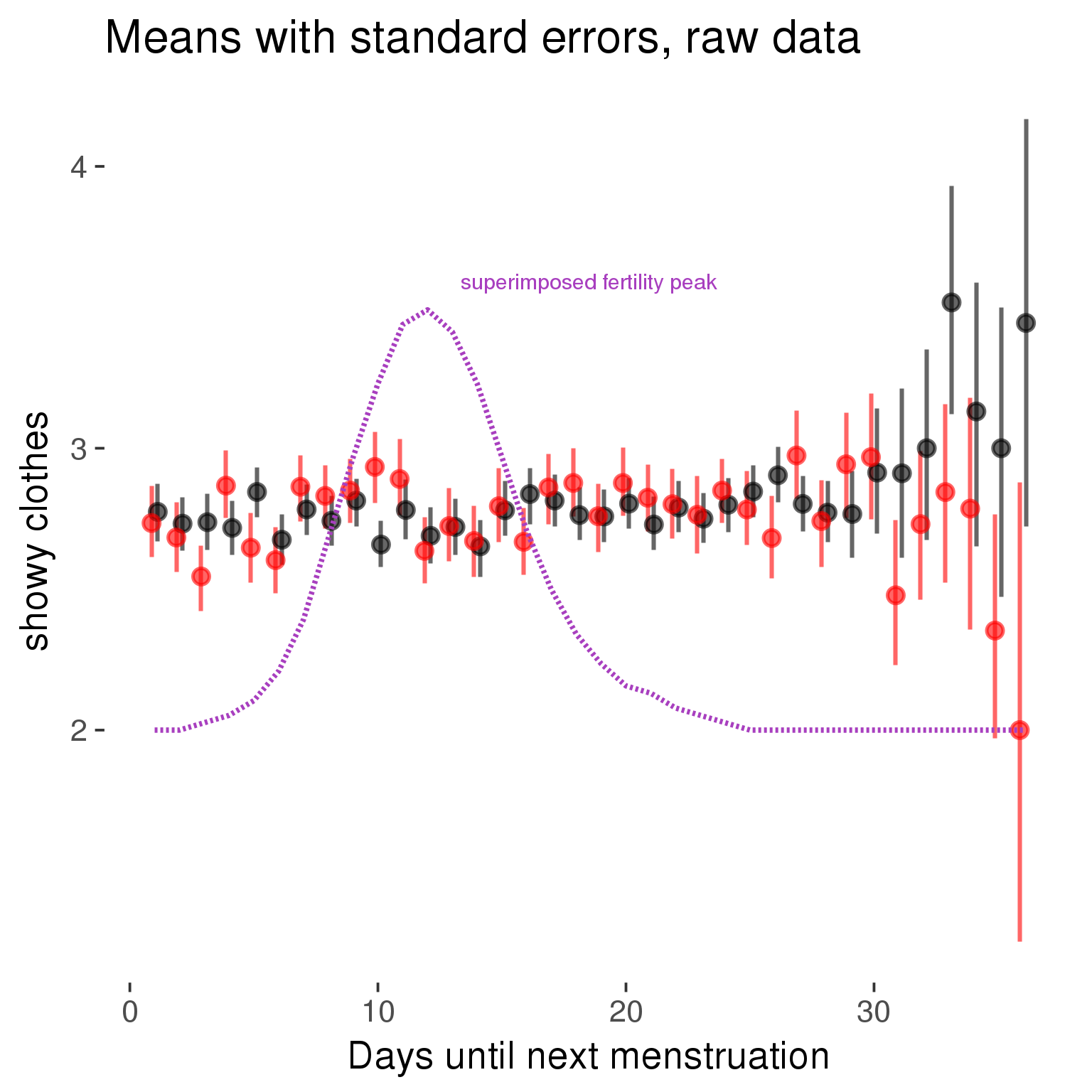
Cycle lengths from 27 to 30
Backward-counted
model %>%
plot_curve(diary %>% filter(minimum_cycle_length_diary <= 30, minimum_cycle_length_diary >= 27) %>% mutate(fertile=prc_stirn_b))outcome = names(model@frame)[1]
outcome_label = recode(str_replace_all(str_replace_all(str_replace_all(outcome, "_", " "), " pair", "-pair"), " 1", ""),
"desirability 1" = "self-perceived desirability",
"NARQ admiration" = "narcissistic admiration",
"NARQ rivalry" = "narcissistic rivalry",
"extra-pair" = "extra-pair desire & behaviour",
"had sexual intercourse" = "sexual intercourse")
library(ggplot2)
# form a subset and run the model without the hormonal contraception and the fertility predictors
tmp = diary %>%
filter(!is.na(fertile), !is.na(included),
RCD > -1 * minimum_cycle_length_diary, RCD > -40)
new_form = update.formula(formula(model), new = . ~ . - fertile * included)
tmp$residuals = residuals(update(model, new_form, data = tmp , na.action = na.exclude))
tmp = tmp %>%
filter(!is.na(RCD), !is.na(residuals))
rcd_min = min(tmp$RCD)
tmp$real = FALSE
tmp_before = tmp
tmp_before$RCD = tmp_before$RCD + min(tmp$RCD) - 1
tmp_after = tmp
tmp_after$RCD = tmp_after$RCD - min(tmp$RCD) + 1
tmp$real = TRUE
tmp = bind_rows(tmp_before %>% filter(RCD > rcd_min - 11), tmp, tmp_after %>% filter(RCD < 11))GAM smooth on residuals
Here, we partialled out menstruation and individual random effects, then superimposed estimated probability of being in the fertile window scaled to the range of the estimated means. To address the periodicity of the cycle, we prepended and appended ten days of the timeseries to the end and the beginning of the timeseries. We then estimated the GAM and cut off the appended subsets before plotting.
tryCatch({
trend_plot = ggplot(tmp,aes(x = RCD, y = residuals, colour = included)) +
stat_smooth(geom = 'smooth',size = 0.8, fill = "#9ECAE1", method = 'gam', formula = y ~ s(x))
}, error = function(e){cat_message(e, "danger")})
tryCatch({
trend_data = ggplot_build(trend_plot)$data[[1]]
}, error = function(e){cat_message(e, "danger")})
trend_data$RCD = round(trend_data$x)
trend_data = left_join(trend_data, tmp %>% select(real, RCD,fertile) %>% unique(), by = "RCD")
trend_data %>%
filter(real == TRUE) %>%
mutate(superimposed = ( ( (fertile - 0.01)/0.58) * (max(y)-min(y) ) ) + min(y) ) ->
trend_data
ggplot(trend_data) +
geom_ribbon(aes(x = x, ymin = ymin, ymax = ymax, fill = factor(group)), alpha = 0.2) +
geom_line(aes(x = x, y = y, colour = factor(group)), size = 0.8, stat = "identity") +
scale_x_continuous(caption_x) +
geom_line(aes(x = x, y = superimposed), color = "#a83fbf", size = 1, linetype = 'dashed') +
annotate("text",x = mean(trend_data$x), y = max(trend_data$superimposed,na.rm=T) + 0.1, label = 'superimposed fertility peak', color = "#a83fbf") +
scale_y_continuous(outcome_label) +
ggtitle("GAM smooth, residuals") +
scale_color_manual("Contraception status",values = c("2"="black","1"= "red"), labels = c("2"="hormonally\ncontracepting","1"="cycling"), guide = F) +
scale_fill_manual("Contraception status",values = c("2"="black","1"= "red"), labels = c("2"="hormonally\ncontracepting","1"="cycling"), guide = F)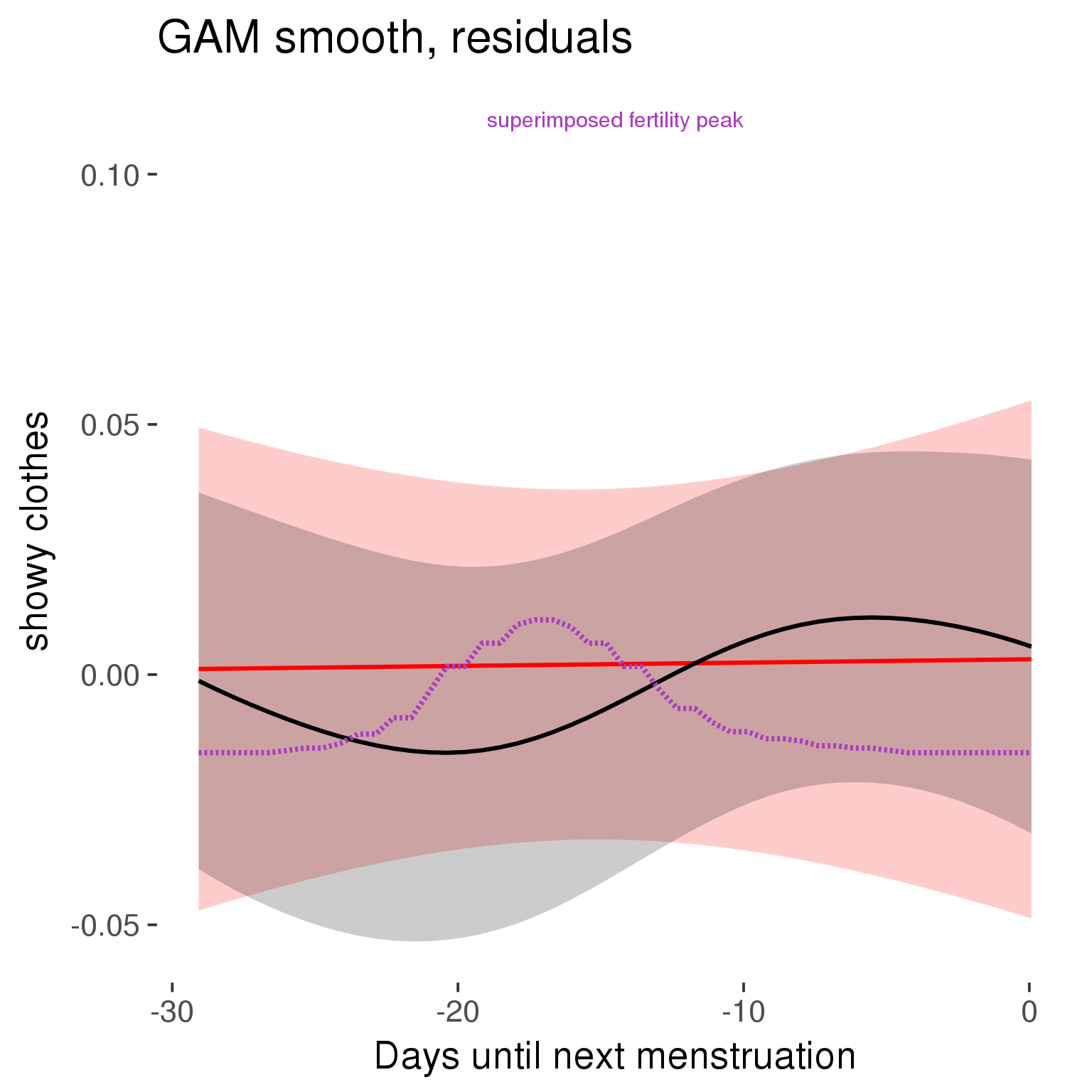
GAM smooth on raw data
As before, but without partialling anything out.
tryCatch({
trend_plot = ggplot(tmp,aes_string(x = "RCD", y = outcome, colour = "included")) +
stat_smooth(geom = 'smooth',size = 0.8, fill = "#9ECAE1", method = 'gam', formula = y ~ s(x))
}, error = function(e){cat_message(e, "danger")})
tryCatch({
trend_data = ggplot_build(trend_plot)$data[[1]]
}, error = function(e){cat_message(e, "danger")})
trend_data$RCD = round(trend_data$x)
trend_data = left_join(trend_data, tmp %>% select(real, RCD,fertile) %>% unique(), by = "RCD")
trend_data %>%
filter(real == TRUE) %>%
mutate(superimposed = ( ( (fertile - 0.01)/0.58) * (max(y)-min(y) ) ) + min(y) ) ->
trend_data
plot1b = ggplot(trend_data) +
geom_ribbon(aes(x = x, ymin = ymin, ymax = ymax, fill = factor(group)), alpha = 0.2) +
geom_line(aes(x = x, y = y, colour = factor(group)), size = 0.8, stat = "identity") +
scale_x_continuous(caption_x) +
geom_line(aes(x = x, y = superimposed), color = "#a83fbf", size = 1, linetype = 'dashed') +
annotate("text",x = mean(trend_data$x), y = max(trend_data$superimposed,na.rm=T) + 0.1, label = 'superimposed fertility peak', color = "#a83fbf") +
scale_y_continuous(outcome_label) +
ggtitle("GAM smooth, raw data") +
scale_color_manual("Contraception status",values = c("2"="black","1"= "red"), labels = c("2"="hormonally\ncontracepting","1"="cycling"), guide = F) +
scale_fill_manual("Contraception status",values = c("2"="black","1"= "red"), labels = c("2"="hormonally\ncontracepting","1"="cycling"), guide = F)
suppressWarnings(print(plot1b))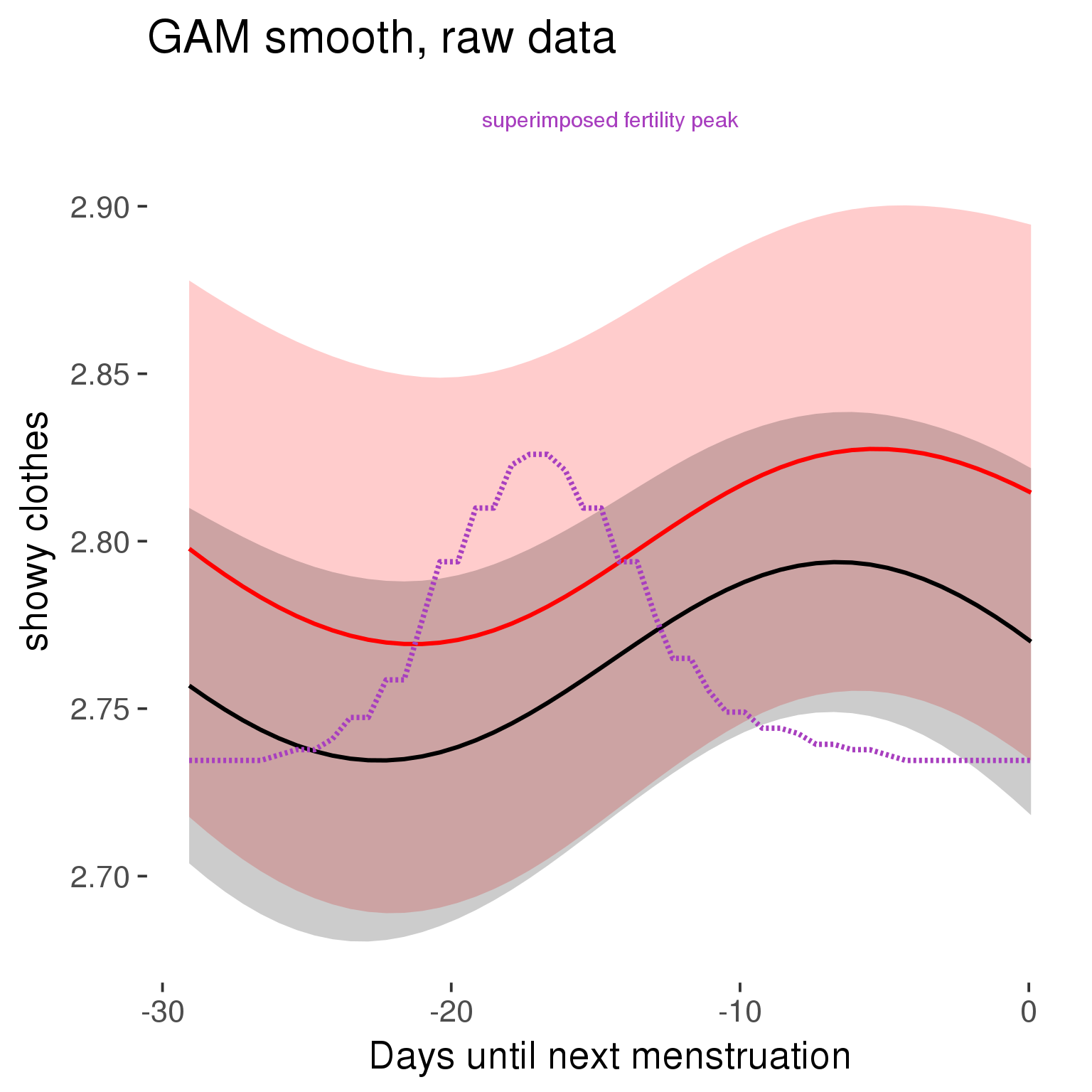
Means and standard errors over raw data
Nothing partialled out, just straight means with bootstrapped confidence intervals.
tryCatch({
trend_plot = ggplot(tmp,aes_string(x = "RCD", y = outcome, colour = "included")) +
geom_pointrange(size = 0.8, stat = 'summary', fun.data = "mean_cl_boot")
}, error = function(e){cat_message(e, "danger")})
tryCatch({
trend_data = ggplot_build(trend_plot)$data[[1]]
}, error = function(e){cat_message(e, "danger")})
trend_data$RCD = round(trend_data$x)
trend_data = left_join(trend_data, tmp %>% select(real, RCD,fertile) %>% unique(), by = "RCD")
trend_data %>%
filter(real == TRUE) %>%
mutate(superimposed = ( ( (fertile - 0.01)/0.58) * (max(y)-min(y) ) ) + min(y) ) ->
trend_data
plot3 = ggplot(trend_data) +
geom_pointrange(aes(x = x, y = y, ymin = ymin,ymax = ymax, colour = factor(group)), size = 0.8, stat = "identity", alpha = 0.6, position = position_dodge(width = .5)) +
scale_x_continuous("Days until next menstruation") +
geom_line(aes(x= x, y = superimposed), color = "#a83fbf", size = 1, linetype = 'dashed') +
annotate("text",x = mean(trend_data$x), y = max(trend_data$superimposed,na.rm=T) + 0.1, label = 'superimposed fertility peak', color = "#a83fbf") +
scale_y_continuous(outcome_label) +
ggtitle("Means with standard errors, raw data") +
scale_color_manual("Contraception status",values = c("2"="black","1"= "red"), labels = c("2"="hormonally\ncontracepting","1"="cycling"), guide = F) +
scale_fill_manual("Contraception status",values = c("2"="black","1"= "red"), labels = c("2"="hormonally\ncontracepting","1"="cycling"), guide = F)
suppressWarnings(print(plot3))
Forward-counted
model %>%
plot_curve(diary %>% filter(minimum_cycle_length_diary <= 30, minimum_cycle_length_diary >= 27) %>% mutate(RCD = FCD, fertile = prc_stirn_b_forward_counted), caption_x = "Days since last menstruation")outcome = names(model@frame)[1]
outcome_label = recode(str_replace_all(str_replace_all(str_replace_all(outcome, "_", " "), " pair", "-pair"), " 1", ""),
"desirability 1" = "self-perceived desirability",
"NARQ admiration" = "narcissistic admiration",
"NARQ rivalry" = "narcissistic rivalry",
"extra-pair" = "extra-pair desire & behaviour",
"had sexual intercourse" = "sexual intercourse")
library(ggplot2)
# form a subset and run the model without the hormonal contraception and the fertility predictors
tmp = diary %>%
filter(!is.na(fertile), !is.na(included),
RCD > -1 * minimum_cycle_length_diary, RCD > -40)
new_form = update.formula(formula(model), new = . ~ . - fertile * included)
tmp$residuals = residuals(update(model, new_form, data = tmp , na.action = na.exclude))
tmp = tmp %>%
filter(!is.na(RCD), !is.na(residuals))
rcd_min = min(tmp$RCD)
tmp$real = FALSE
tmp_before = tmp
tmp_before$RCD = tmp_before$RCD + min(tmp$RCD) - 1
tmp_after = tmp
tmp_after$RCD = tmp_after$RCD - min(tmp$RCD) + 1
tmp$real = TRUE
tmp = bind_rows(tmp_before %>% filter(RCD > rcd_min - 11), tmp, tmp_after %>% filter(RCD < 11))GAM smooth on residuals
Here, we partialled out menstruation and individual random effects, then superimposed estimated probability of being in the fertile window scaled to the range of the estimated means. To address the periodicity of the cycle, we prepended and appended ten days of the timeseries to the end and the beginning of the timeseries. We then estimated the GAM and cut off the appended subsets before plotting.
tryCatch({
trend_plot = ggplot(tmp,aes(x = RCD, y = residuals, colour = included)) +
stat_smooth(geom = 'smooth',size = 0.8, fill = "#9ECAE1", method = 'gam', formula = y ~ s(x))
}, error = function(e){cat_message(e, "danger")})
tryCatch({
trend_data = ggplot_build(trend_plot)$data[[1]]
}, error = function(e){cat_message(e, "danger")})
trend_data$RCD = round(trend_data$x)
trend_data = left_join(trend_data, tmp %>% select(real, RCD,fertile) %>% unique(), by = "RCD")
trend_data %>%
filter(real == TRUE) %>%
mutate(superimposed = ( ( (fertile - 0.01)/0.58) * (max(y)-min(y) ) ) + min(y) ) ->
trend_data
ggplot(trend_data) +
geom_ribbon(aes(x = x, ymin = ymin, ymax = ymax, fill = factor(group)), alpha = 0.2) +
geom_line(aes(x = x, y = y, colour = factor(group)), size = 0.8, stat = "identity") +
scale_x_continuous(caption_x) +
geom_line(aes(x = x, y = superimposed), color = "#a83fbf", size = 1, linetype = 'dashed') +
annotate("text",x = mean(trend_data$x), y = max(trend_data$superimposed,na.rm=T) + 0.1, label = 'superimposed fertility peak', color = "#a83fbf") +
scale_y_continuous(outcome_label) +
ggtitle("GAM smooth, residuals") +
scale_color_manual("Contraception status",values = c("2"="black","1"= "red"), labels = c("2"="hormonally\ncontracepting","1"="cycling"), guide = F) +
scale_fill_manual("Contraception status",values = c("2"="black","1"= "red"), labels = c("2"="hormonally\ncontracepting","1"="cycling"), guide = F)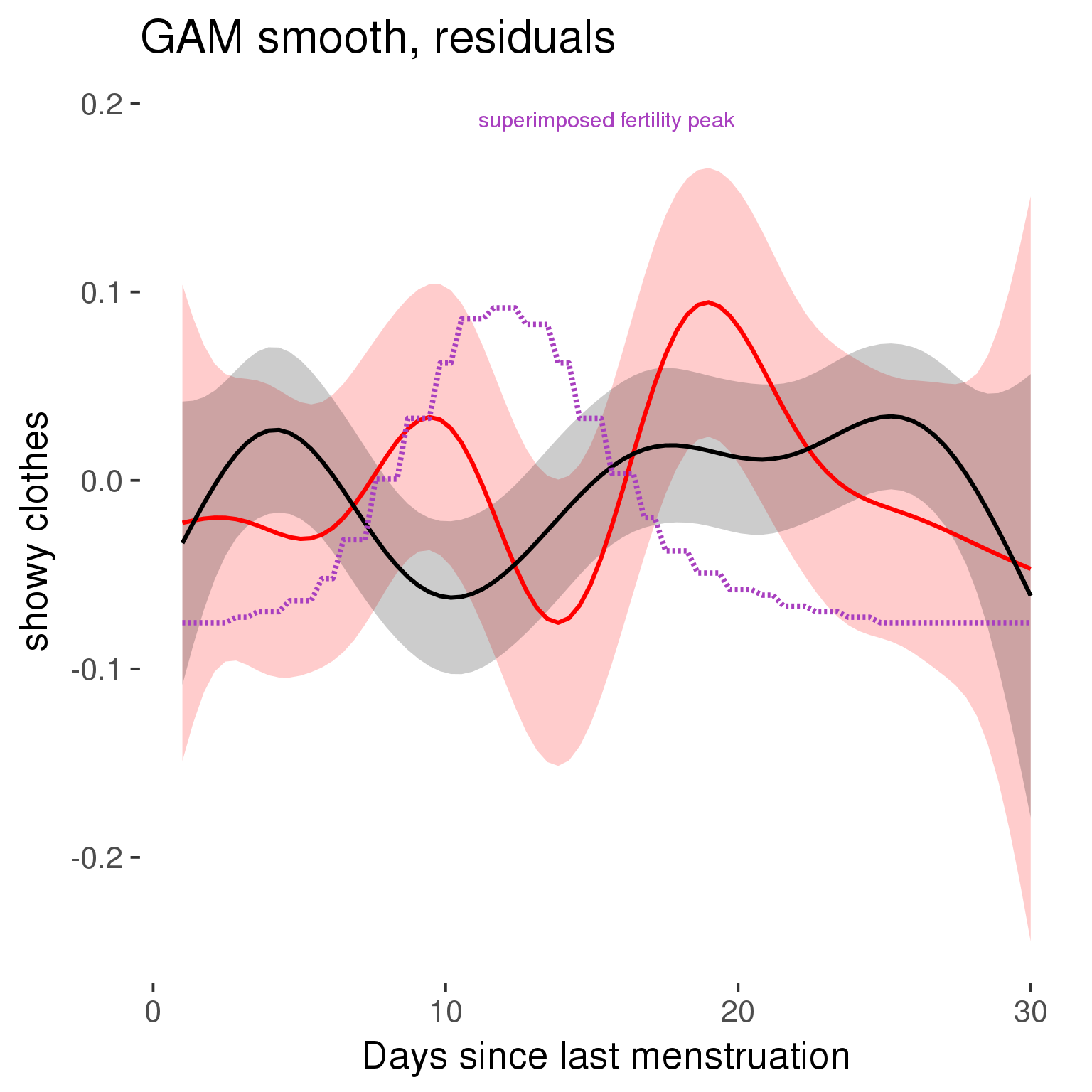
GAM smooth on raw data
As before, but without partialling anything out.
tryCatch({
trend_plot = ggplot(tmp,aes_string(x = "RCD", y = outcome, colour = "included")) +
stat_smooth(geom = 'smooth',size = 0.8, fill = "#9ECAE1", method = 'gam', formula = y ~ s(x))
}, error = function(e){cat_message(e, "danger")})
tryCatch({
trend_data = ggplot_build(trend_plot)$data[[1]]
}, error = function(e){cat_message(e, "danger")})
trend_data$RCD = round(trend_data$x)
trend_data = left_join(trend_data, tmp %>% select(real, RCD,fertile) %>% unique(), by = "RCD")
trend_data %>%
filter(real == TRUE) %>%
mutate(superimposed = ( ( (fertile - 0.01)/0.58) * (max(y)-min(y) ) ) + min(y) ) ->
trend_data
plot1b = ggplot(trend_data) +
geom_ribbon(aes(x = x, ymin = ymin, ymax = ymax, fill = factor(group)), alpha = 0.2) +
geom_line(aes(x = x, y = y, colour = factor(group)), size = 0.8, stat = "identity") +
scale_x_continuous(caption_x) +
geom_line(aes(x = x, y = superimposed), color = "#a83fbf", size = 1, linetype = 'dashed') +
annotate("text",x = mean(trend_data$x), y = max(trend_data$superimposed,na.rm=T) + 0.1, label = 'superimposed fertility peak', color = "#a83fbf") +
scale_y_continuous(outcome_label) +
ggtitle("GAM smooth, raw data") +
scale_color_manual("Contraception status",values = c("2"="black","1"= "red"), labels = c("2"="hormonally\ncontracepting","1"="cycling"), guide = F) +
scale_fill_manual("Contraception status",values = c("2"="black","1"= "red"), labels = c("2"="hormonally\ncontracepting","1"="cycling"), guide = F)
suppressWarnings(print(plot1b))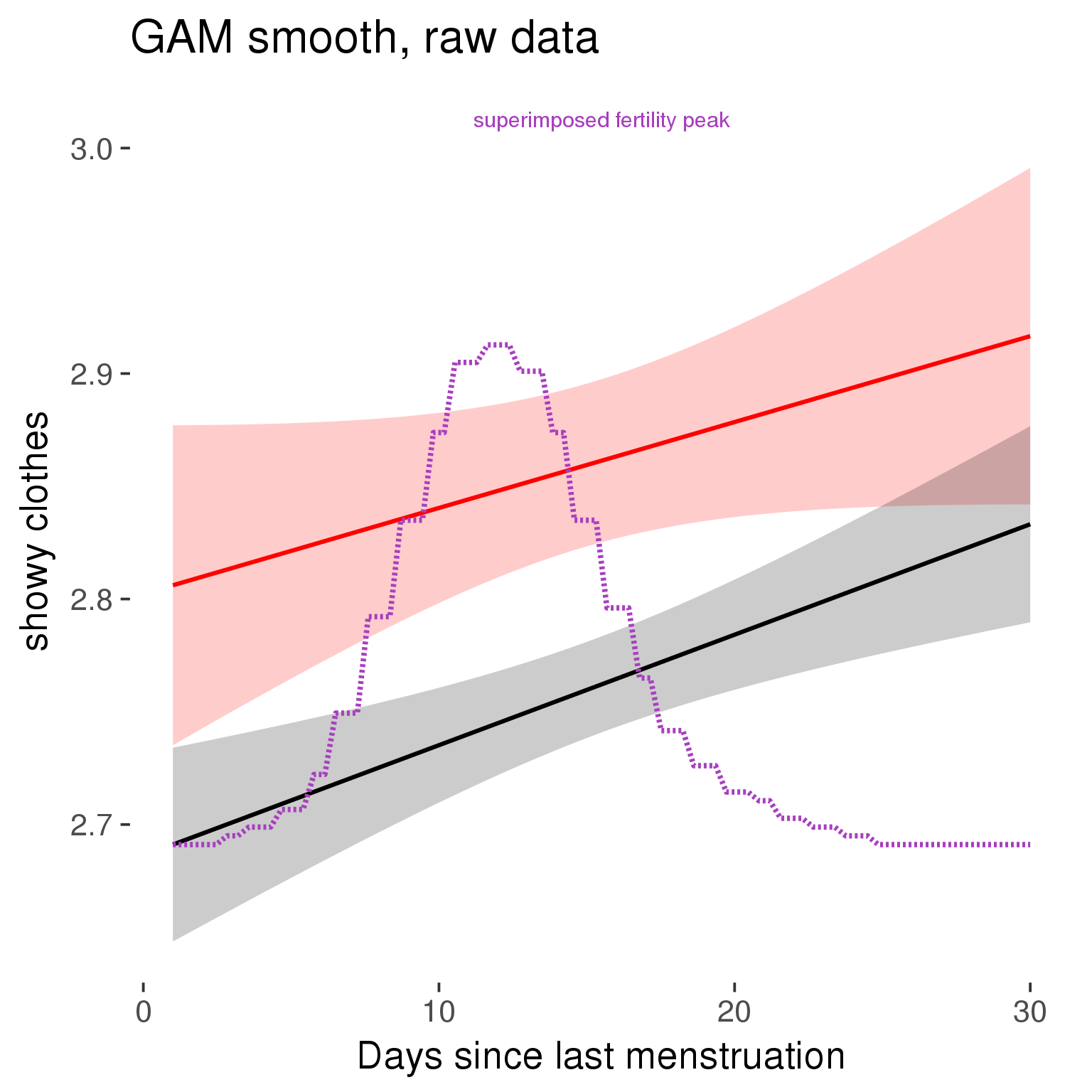
Means and standard errors over raw data
Nothing partialled out, just straight means with bootstrapped confidence intervals.
tryCatch({
trend_plot = ggplot(tmp,aes_string(x = "RCD", y = outcome, colour = "included")) +
geom_pointrange(size = 0.8, stat = 'summary', fun.data = "mean_cl_boot")
}, error = function(e){cat_message(e, "danger")})
tryCatch({
trend_data = ggplot_build(trend_plot)$data[[1]]
}, error = function(e){cat_message(e, "danger")})
trend_data$RCD = round(trend_data$x)
trend_data = left_join(trend_data, tmp %>% select(real, RCD,fertile) %>% unique(), by = "RCD")
trend_data %>%
filter(real == TRUE) %>%
mutate(superimposed = ( ( (fertile - 0.01)/0.58) * (max(y)-min(y) ) ) + min(y) ) ->
trend_data
plot3 = ggplot(trend_data) +
geom_pointrange(aes(x = x, y = y, ymin = ymin,ymax = ymax, colour = factor(group)), size = 0.8, stat = "identity", alpha = 0.6, position = position_dodge(width = .5)) +
scale_x_continuous("Days until next menstruation") +
geom_line(aes(x= x, y = superimposed), color = "#a83fbf", size = 1, linetype = 'dashed') +
annotate("text",x = mean(trend_data$x), y = max(trend_data$superimposed,na.rm=T) + 0.1, label = 'superimposed fertility peak', color = "#a83fbf") +
scale_y_continuous(outcome_label) +
ggtitle("Means with standard errors, raw data") +
scale_color_manual("Contraception status",values = c("2"="black","1"= "red"), labels = c("2"="hormonally\ncontracepting","1"="cycling"), guide = F) +
scale_fill_manual("Contraception status",values = c("2"="black","1"= "red"), labels = c("2"="hormonally\ncontracepting","1"="cycling"), guide = F)
suppressWarnings(print(plot3))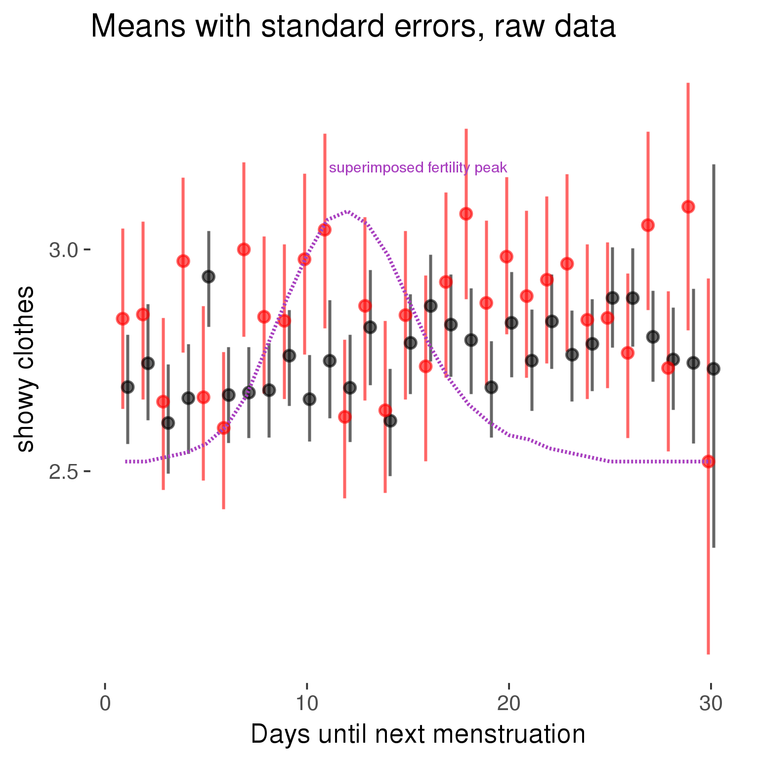
Robustness checks
M_r1: Random slopes for conception risk and menstruation
tryCatch({
# refit model with random effects for fertile and menstruation dummies
with_ind_diff = update(model, formula = . ~ . - (1| person) + (1 + fertile + menstruation | person))
# pull the random effects, format as tibble
rand = coef(with_ind_diff)$person %>%
tibble::rownames_to_column("person") %>%
mutate(person = as.numeric(person))
# pull the fixed effects
fixd = data.frame(fixef(with_ind_diff)) %>%
tibble::rownames_to_column("effect")
names(fixd) = c("effect", "pop_effect_size")
# pull apart the coefficients so that we can account for the fact that the random effect variation implicitly includes HC explaining the mean population-level effect of fertile/menstruation dummies among HC users
fixd = fixd %>%
separate(effect, c("included", "effect"), sep = ":", fill = "left") %>%
mutate(included = if_else(is.na(included), "cycling", str_replace(included, "included", "")))
fixd[2,c("included", "effect")] = c("horm_contra", "(Intercept)")
rand = rand %>%
# merge diary data on the random effects, so that we know who is a HC users and who isn't
inner_join(diary %>% select(person, included) %>% unique(), by = 'person') %>%
# gather into long format, to have the dataset by predictor
gather(effect, value, -person, -included) %>%
inner_join(fixd, by = c('effect', 'included')) %>%
# pull the fixed effects
mutate(
# only for those who are HC users, add the moderated population effect size for this effect (the random effects have the reference category mean)
value = if_else(included == "horm_contra", value + pop_effect_size, value),
effect = recode(effect, "includedhorm_contra" = "HC user",
"includedhorm_contra:fertile" = "HC user x fertile",
"includedhorm_contra:menstruationpre" = "HC user x premens.",
"includedhorm_contra:menstruationyes" = "HC user x mens.",
"menstruationyes" = "mens.",
"menstruationpre" = "premens.")) %>%
group_by(included, effect) %>%
# filter out predictors that aren't modelled as varying/random
filter(sd(value) > 0)
# plot dot plot of random effects
print(
ggplot(rand, aes(x = included, y = value, color = included, fill = included)) +
facet_wrap( ~ effect, scales = "free") +
# geom_violin(alpha = 0.4, size = 0) +
geom_dotplot(binaxis='y', dotsize = 0.1, method = "histodot") +
# geom_jitter(alpha = 0.05) +
coord_flip() +
geom_pointrange(stat = 'summary', fun.data = 'mean_sdl', color = 'darkred', size = 1.2) +
scale_color_manual("Contraception status", values = c("horm_contra"="black","cycling"= "red"), labels = c("horm_contra"="hormonally\ncontracepting","cycling"="cycling"), guide = F) +
scale_fill_manual("Contraception status", values = c("horm_contra"="black","cycling"= "red"), labels = c("horm_contra"="hormonally\ncontracepting","1"="cycling"), guide = F) +
ggtitle("M_r1: allowing participant-varying slopes", subtitle = "for the conception risk measure and the menstruation dummies") +
scale_x_discrete("Hormonal contraception", breaks = c("horm_contra", "cycling"), labels = c("yes", "no")) +
scale_y_continuous("Random effect size distribution"))
print_summary(with_ind_diff)
cat(pander(anova(model, with_ind_diff)))
}, error = function(e){
with_ind_diff = model
cat_message(e, "danger")
})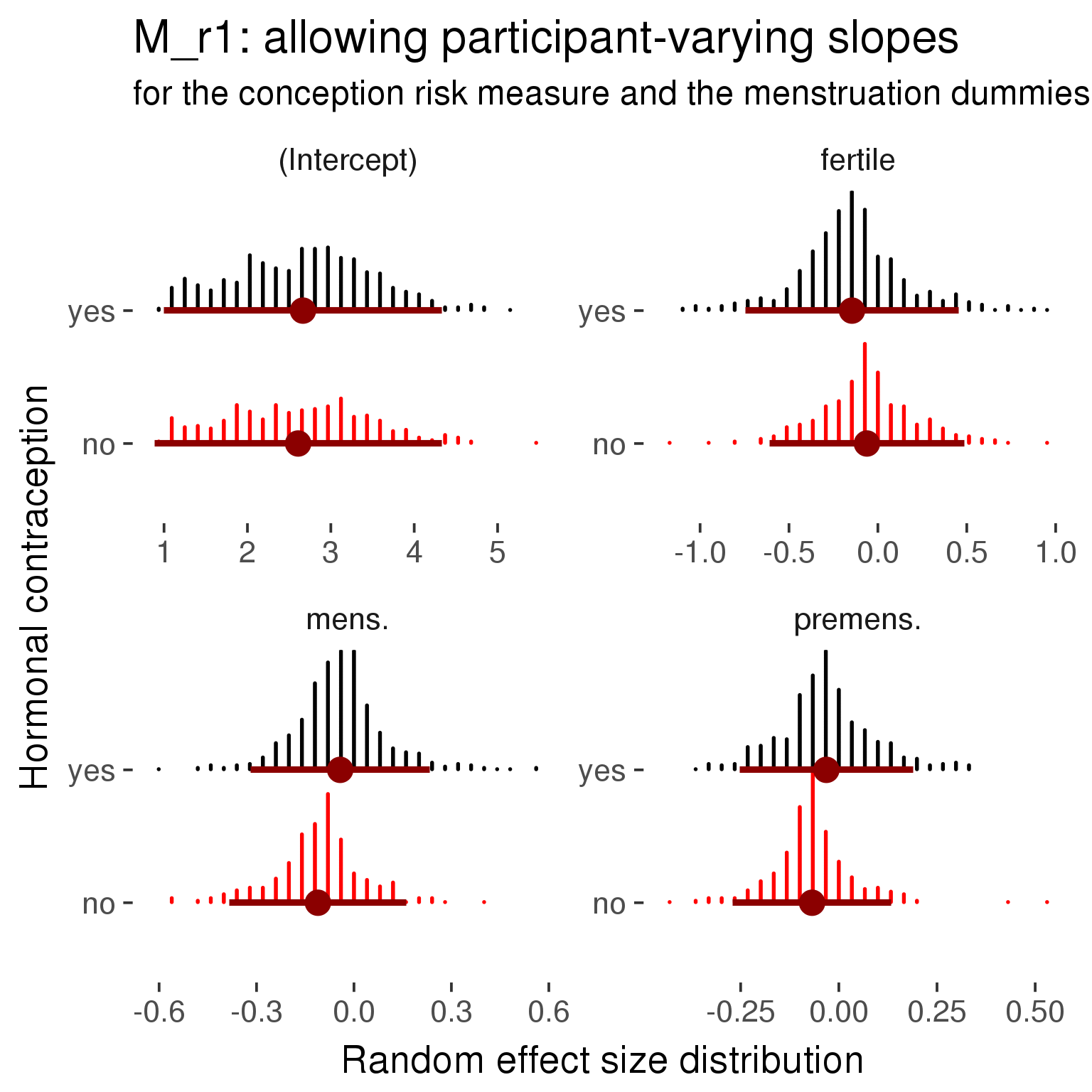
Linear mixed model fit by REML ['lmerMod']
Formula: showy_clothes ~ included + menstruation + fertile + fertile_mean +
(1 + fertile + menstruation | person) + included:menstruation + included:fertile
Data: diary
REML criterion at convergence: 84560
Scaled residuals:
Min 1Q Median 3Q Max
-3.553 -0.618 -0.099 0.620 3.993
Random effects:
Groups Name Variance Std.Dev. Corr
person (Intercept) 0.8275 0.910
fertile 0.4417 0.665 -0.10
menstruationpre 0.0804 0.283 -0.02 0.25
menstruationyes 0.1039 0.322 -0.18 0.23 0.27
Residual 1.2225 1.106
Number of obs: 26685, groups: person, 1054
Fixed effects:
Estimate Std. Error t value
(Intercept) 2.6080 0.0795 32.8
includedhorm_contra 0.0578 0.0653 0.9
menstruationpre -0.0681 0.0379 -1.8
menstruationyes -0.1110 0.0370 -3.0
fertile -0.0617 0.0785 -0.8
fertile_mean 0.6050 0.3654 1.7
includedhorm_contra:menstruationpre 0.0364 0.0486 0.7
includedhorm_contra:menstruationyes 0.0685 0.0483 1.4
includedhorm_contra:fertile -0.0840 0.0996 -0.8
Correlation of Fixed Effects:
(Intr) incld_ mnstrtnp mnstrtny fertil frtl_m inclddhrm_cntr:mnstrtnp
inclddhrm_c -0.475
menstrutnpr -0.155 0.197
menstrutnys -0.193 0.236 0.365
fertile -0.162 0.267 0.417 0.347
fertile_men -0.770 -0.027 -0.009 0.000 -0.073
inclddhrm_cntr:mnstrtnp 0.129 -0.246 -0.779 -0.285 -0.324 -0.004
inclddhrm_cntr:mnstrtny 0.153 -0.293 -0.280 -0.766 -0.266 -0.006 0.354
inclddhrm_cntr:f 0.162 -0.337 -0.328 -0.274 -0.785 0.012 0.417
inclddhrm_cntr:mnstrtny
inclddhrm_c
menstrutnpr
menstrutnys
fertile
fertile_men
inclddhrm_cntr:mnstrtnp
inclddhrm_cntr:mnstrtny
inclddhrm_cntr:f 0.344
refitting model(s) with ML (instead of REML)
| Df | AIC | BIC | logLik | deviance | Chisq | Chi Df | Pr(>Chisq) | |
|---|---|---|---|---|---|---|---|---|
| object | 11 | 84648 | 84738 | -42313 | 84626 | NA | NA | NA |
| ..1 | 20 | 84563 | 84727 | -42261 | 84523 | 102.8 | 9 | 4.2e-18 |
robustness_check_ovu_shift(model, diary)M_e: Exclusion criteria
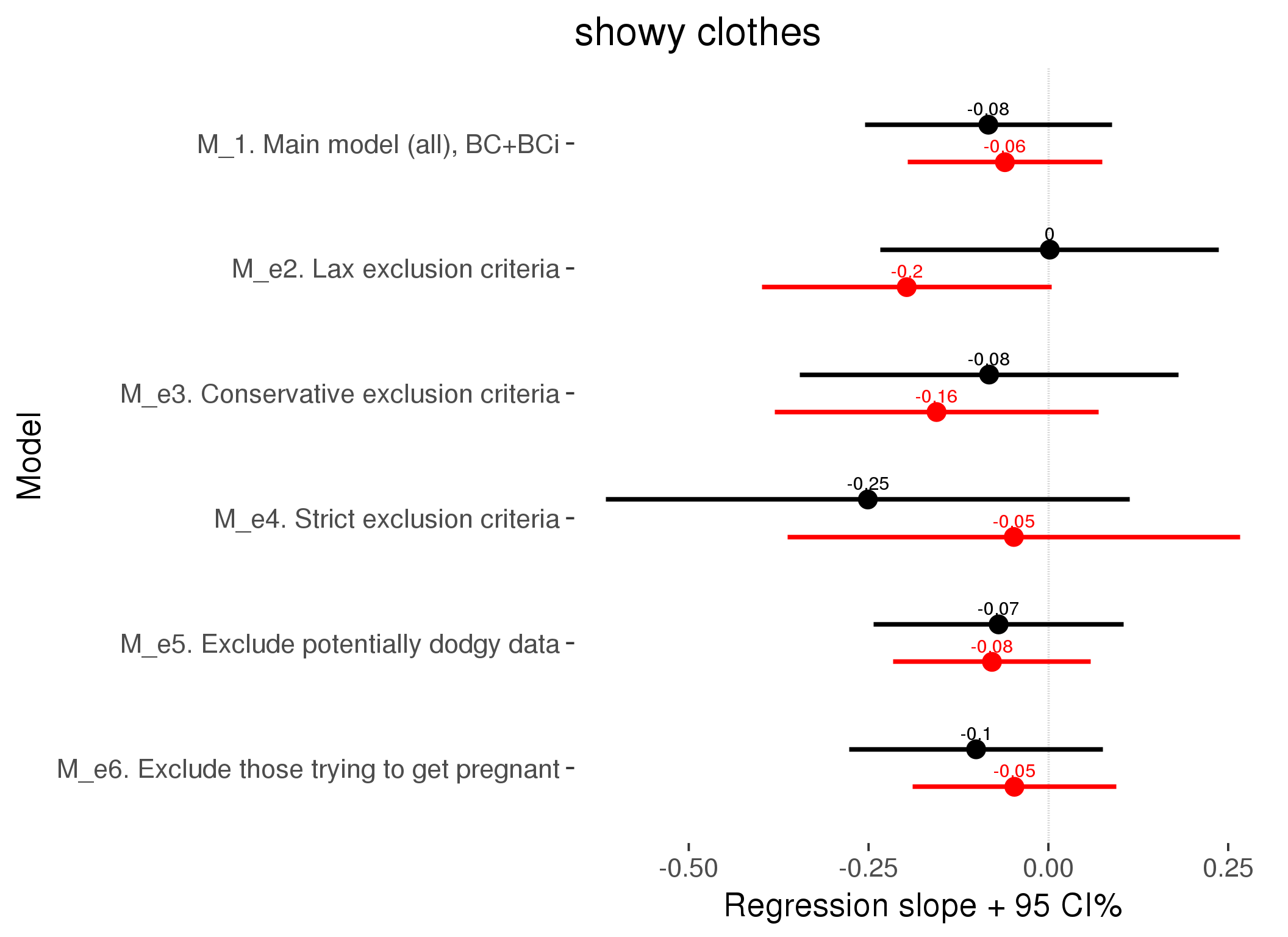
M_p: Predictors
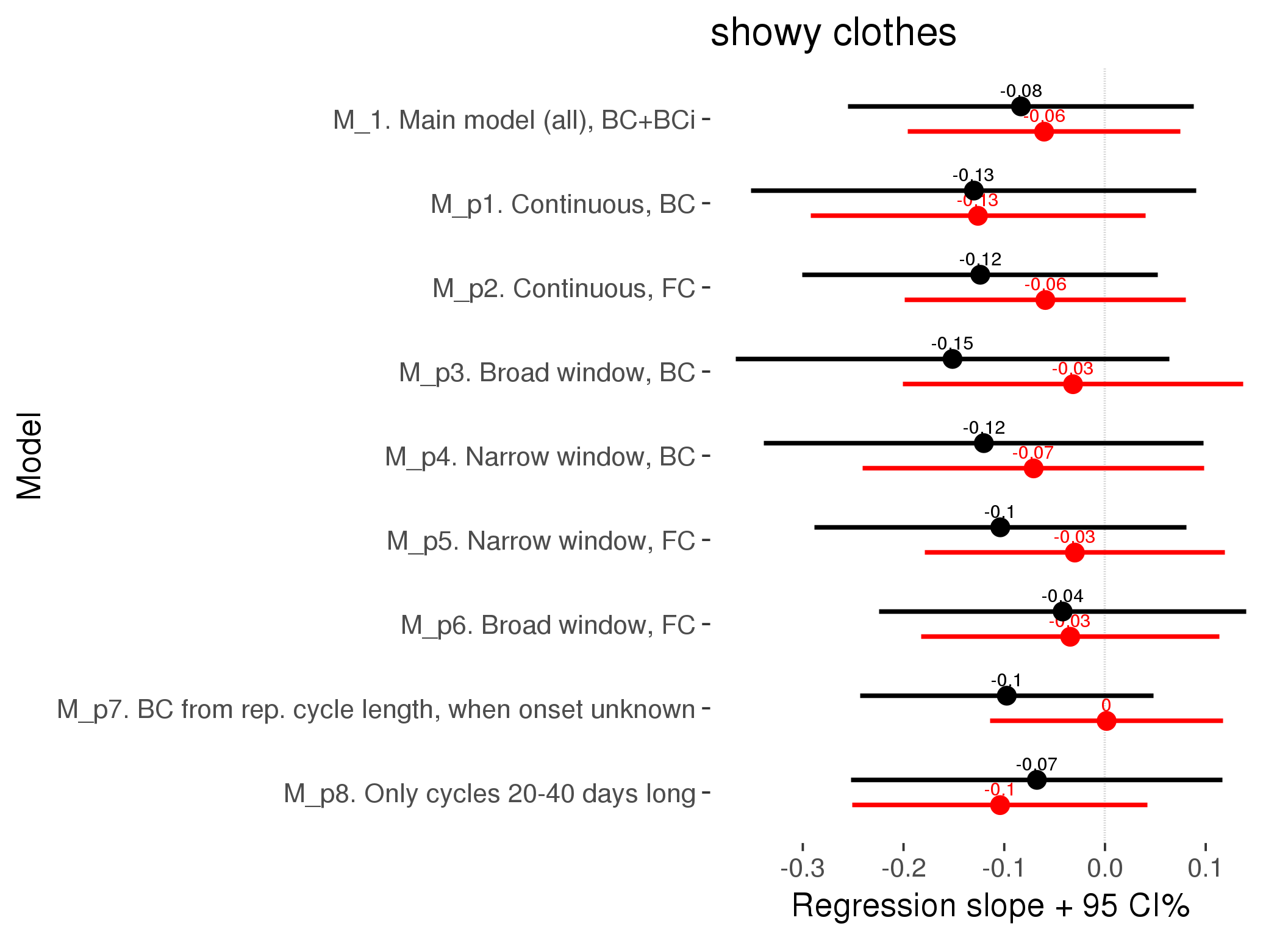
M_c: Covariates, controls, autocorrelation
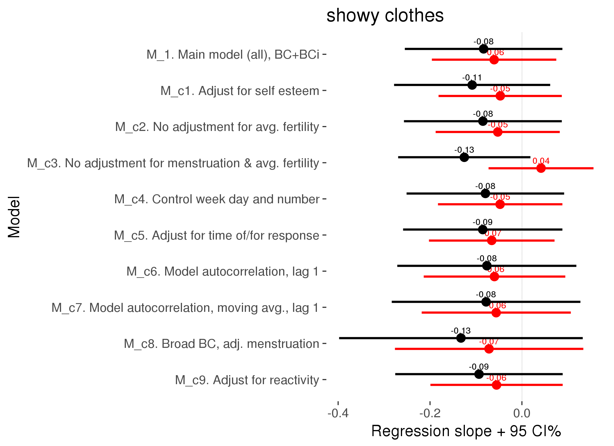
Linear mixed model fit by REML ['lmerMod']
REML criterion at convergence: 77426
Scaled residuals:
Min 1Q Median 3Q Max
-3.617 -0.634 -0.101 0.626 4.171
Random effects:
Groups Name Variance Std.Dev.
person (Intercept) 7.98e-01 0.8934751106
Xr.2 s(days_filled_out):includedhorm_contra 1.56e-16 0.0000000125
Xr.1 s(days_filled_out):includedcycling 1.58e-02 0.1256428604
Xr.0 s(day_number):includedhorm_contra 7.86e-03 0.0886308686
Xr s(day_number):includedcycling 5.02e-14 0.0000002240
Residual 1.25e+00 1.1197819820
Number of obs: 24382, groups: person, 1054; Xr.2, 8; Xr.1, 8; Xr.0, 8; Xr, 8
Fixed effects:
Estimate Std. Error t value
X(Intercept) 2.6170 0.0791 33.1
Xincludedhorm_contra 0.0670 0.0653 1.0
Xmenstruationpre -0.0570 0.0357 -1.6
Xmenstruationyes -0.0724 0.0343 -2.1
Xfertile -0.0552 0.0735 -0.8
Xfertile_mean 0.5925 0.3612 1.6
Xincludedhorm_contra:menstruationpre 0.0318 0.0458 0.7
Xincludedhorm_contra:menstruationyes 0.0241 0.0449 0.5
Xincludedhorm_contra:fertile -0.0934 0.0931 -1.0
Xs(day_number):includedcyclingFx1 -0.0554 0.0582 -1.0
Xs(day_number):includedhorm_contraFx1 -0.0618 0.0580 -1.1
Xs(days_filled_out):includedcyclingFx1 0.1233 0.0740 1.7
Xs(days_filled_out):includedhorm_contraFx1 0.1391 0.0502 2.8
Family: gaussian
Link function: identity
Formula:
showy_clothes ~ included + menstruation + fertile + fertile_mean +
s(day_number, by = included) + s(days_filled_out, by = included) +
included:menstruation + included:fertile
Parametric coefficients:
Estimate Std. Error t value Pr(>|t|)
(Intercept) 2.6170 0.0791 33.07 <2e-16 ***
includedhorm_contra 0.0670 0.0653 1.03 0.305
menstruationpre -0.0570 0.0357 -1.60 0.110
menstruationyes -0.0724 0.0343 -2.11 0.035 *
fertile -0.0552 0.0735 -0.75 0.452
fertile_mean 0.5925 0.3612 1.64 0.101
includedhorm_contra:menstruationpre 0.0318 0.0458 0.69 0.488
includedhorm_contra:menstruationyes 0.0241 0.0449 0.54 0.591
includedhorm_contra:fertile -0.0934 0.0931 -1.00 0.316
---
Signif. codes: 0 '***' 0.001 '**' 0.01 '*' 0.05 '.' 0.1 ' ' 1
Approximate significance of smooth terms:
edf Ref.df F p-value
s(day_number):includedcycling 1.00 1.00 0.91 0.3412
s(day_number):includedhorm_contra 2.33 2.33 3.25 0.0435 *
s(days_filled_out):includedcycling 2.46 2.46 5.03 0.0031 **
s(days_filled_out):includedhorm_contra 1.00 1.00 7.69 0.0056 **
---
Signif. codes: 0 '***' 0.001 '**' 0.01 '*' 0.05 '.' 0.1 ' ' 1
R-sq.(adj) = 0.00479
lmer.REML = 77426 Scale est. = 1.2539 n = 24382
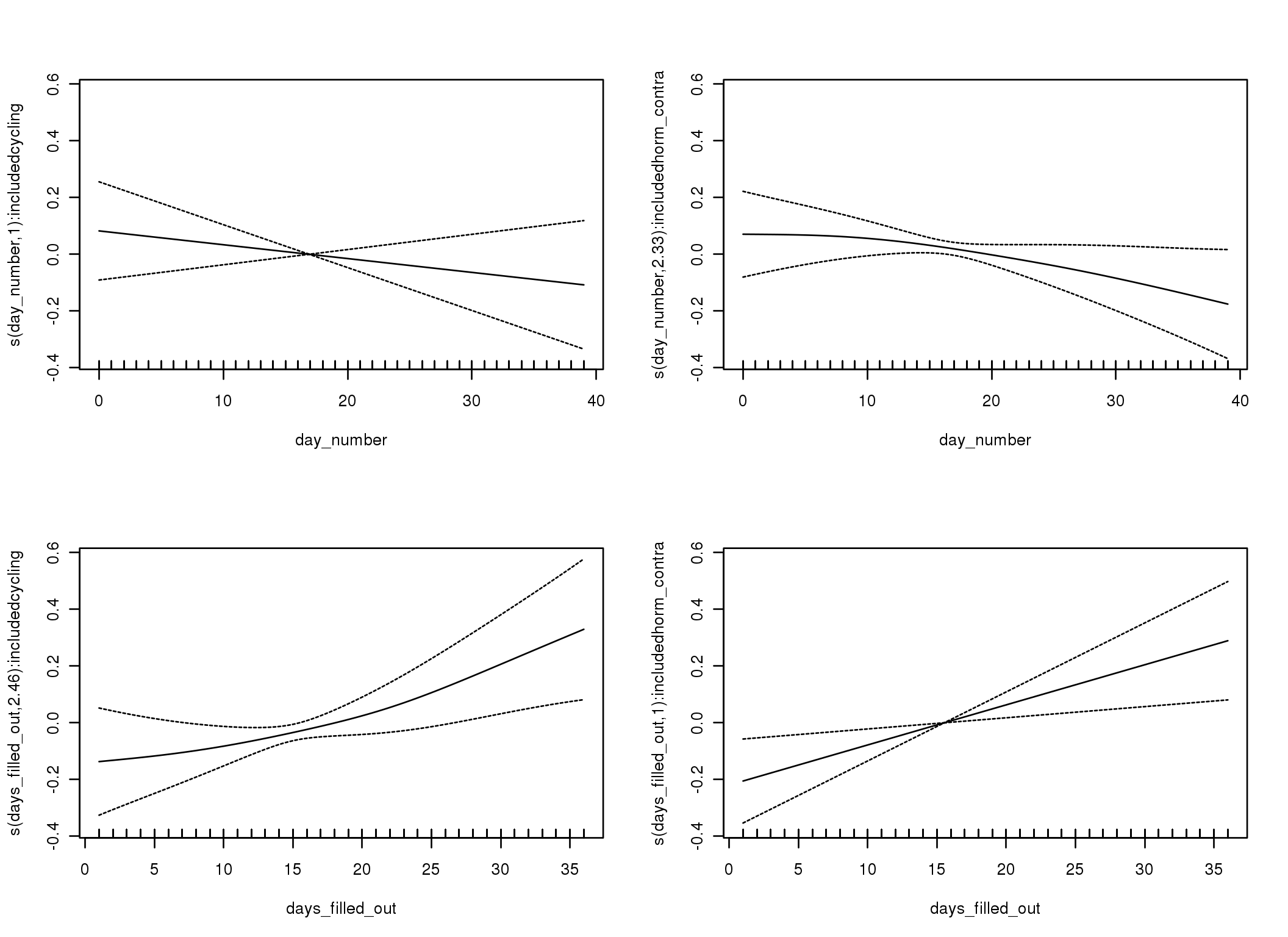
Linear mixed-effects model fit by REML
Data: diary
AIC BIC logLik
84006 84104 -41991
Random effects:
Formula: ~1 | person
(Intercept) Residual
StdDev: 0.8893 1.13
Correlation Structure: ARMA(1,0)
Formula: ~day_number | person
Parameter estimate(s):
Phi1
0.1887
Fixed effects: showy_clothes ~ included * (menstruation + fertile) + fertile_mean
Value Std.Error DF t-value p-value
(Intercept) 2.6142 0.0799 25625 32.70 0.0000
includedhorm_contra 0.0533 0.0657 1051 0.81 0.4171
menstruationpre -0.0717 0.0379 25625 -1.89 0.0584
menstruationyes -0.1182 0.0355 25625 -3.33 0.0009
fertile -0.0599 0.0785 25625 -0.76 0.4461
fertile_mean 0.5995 0.3669 1051 1.63 0.1026
includedhorm_contra:menstruationpre 0.0402 0.0486 25625 0.83 0.4083
includedhorm_contra:menstruationyes 0.0740 0.0464 25625 1.60 0.1103
includedhorm_contra:fertile -0.0763 0.0994 25625 -0.77 0.4429
Correlation:
(Intr) incld_ mnstrtnp mnstrtny fertil frtl_m inclddhrm_cntr:mnstrtnp
includedhorm_contra -0.476
menstruationpre -0.182 0.228
menstruationyes -0.177 0.221 0.399
fertile -0.174 0.286 0.446 0.372
fertile_mean -0.769 -0.026 -0.008 -0.005 -0.077
includedhorm_contra:menstruationpre 0.149 -0.286 -0.779 -0.311 -0.346 -0.004
includedhorm_contra:menstruationyes 0.142 -0.271 -0.306 -0.765 -0.284 -0.004 0.385
includedhorm_contra:fertile 0.175 -0.362 -0.352 -0.293 -0.786 0.012 0.445
inclddhrm_cntr:mnstrtny
includedhorm_contra
menstruationpre
menstruationyes
fertile
fertile_mean
includedhorm_contra:menstruationpre
includedhorm_contra:menstruationyes
includedhorm_contra:fertile 0.367
Standardized Within-Group Residuals:
Min Q1 Med Q3 Max
-3.6749 -0.6259 -0.1099 0.6222 4.0613
Number of Observations: 26685
Number of Groups: 1054
Linear mixed-effects model fit by REML
Data: diary
AIC BIC logLik
83862 83969 -41918
Random effects:
Formula: ~1 | person
(Intercept) Residual
StdDev: 0.8739 1.14
Correlation Structure: ARMA(1,1)
Formula: ~day_number | person
Parameter estimate(s):
Phi1 Theta1
0.6835 -0.5172
Fixed effects: showy_clothes ~ included * (menstruation + fertile) + fertile_mean
Value Std.Error DF t-value p-value
(Intercept) 2.6103 0.0802 25625 32.56 0.0000
includedhorm_contra 0.0525 0.0660 1051 0.80 0.4258
menstruationpre -0.0634 0.0386 25625 -1.64 0.1003
menstruationyes -0.1148 0.0366 25625 -3.14 0.0017
fertile -0.0560 0.0829 25625 -0.68 0.4988
fertile_mean 0.6155 0.3686 1051 1.67 0.0953
includedhorm_contra:menstruationpre 0.0303 0.0496 25625 0.61 0.5419
includedhorm_contra:menstruationyes 0.0690 0.0477 25625 1.45 0.1478
includedhorm_contra:fertile -0.0780 0.1047 25625 -0.74 0.4564
Correlation:
(Intr) incld_ mnstrtnp mnstrtny fertil frtl_m inclddhrm_cntr:mnstrtnp
includedhorm_contra -0.475
menstruationpre -0.183 0.227
menstruationyes -0.183 0.227 0.420
fertile -0.175 0.292 0.399 0.358
fertile_mean -0.769 -0.028 -0.005 -0.005 -0.083
includedhorm_contra:menstruationpre 0.149 -0.284 -0.778 -0.327 -0.310 -0.004
includedhorm_contra:menstruationyes 0.146 -0.278 -0.322 -0.768 -0.274 -0.003 0.407
includedhorm_contra:fertile 0.178 -0.369 -0.316 -0.283 -0.787 0.014 0.399
inclddhrm_cntr:mnstrtny
includedhorm_contra
menstruationpre
menstruationyes
fertile
fertile_mean
includedhorm_contra:menstruationpre
includedhorm_contra:menstruationyes
includedhorm_contra:fertile 0.353
Standardized Within-Group Residuals:
Min Q1 Med Q3 Max
-3.5930 -0.6239 -0.1175 0.6230 4.0011
Number of Observations: 26685
Number of Groups: 1054
M_d: Other designs
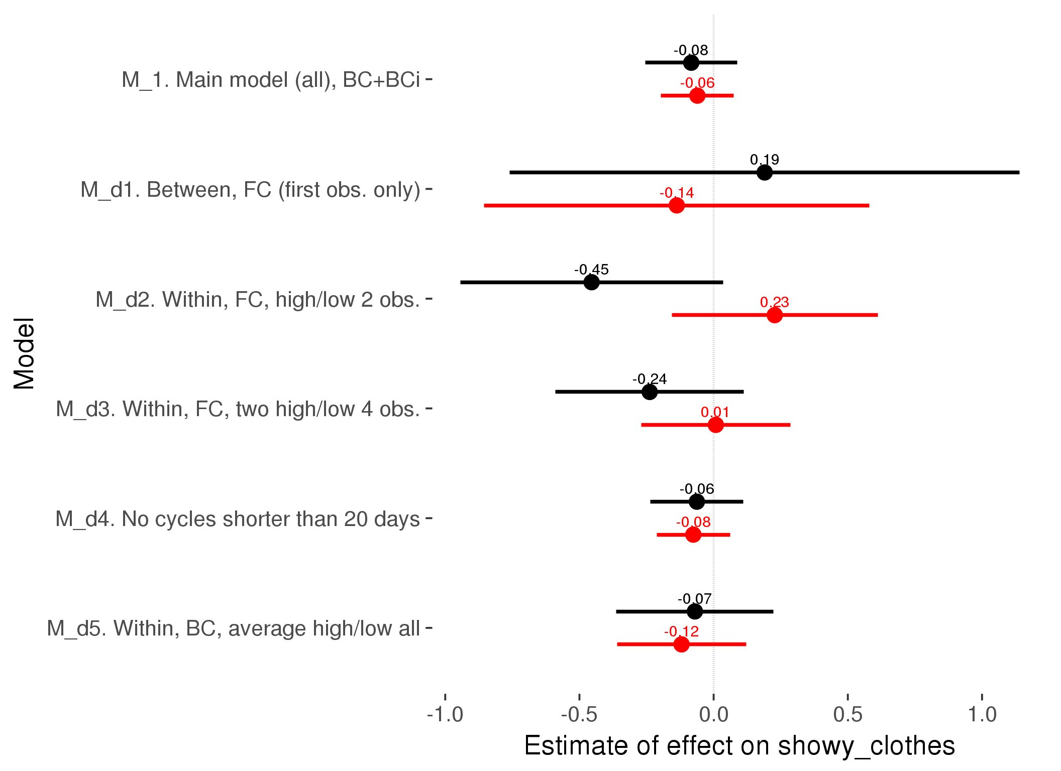
M_m1: Moderation by contraceptive method
Based on the sample with lax exclusion criteria. Users who used any hormonal contraception are classified as hormonal, users who use any awareness-based methods (counting, temperature-based) are classified as ‘fertility-awareness’, women who don’t fall into the before groups and use condoms, pessars, coitus interruptus etc. are classified as ‘barrie or abstinence’. Women who don’t use contraception or use other methods such as sterilisation are excluded from this analysis.
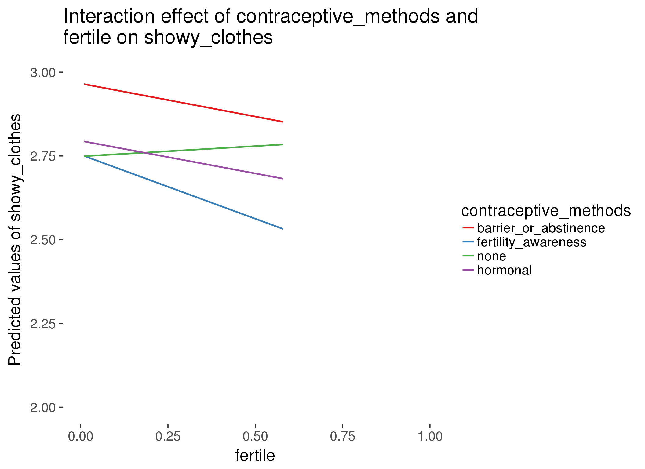
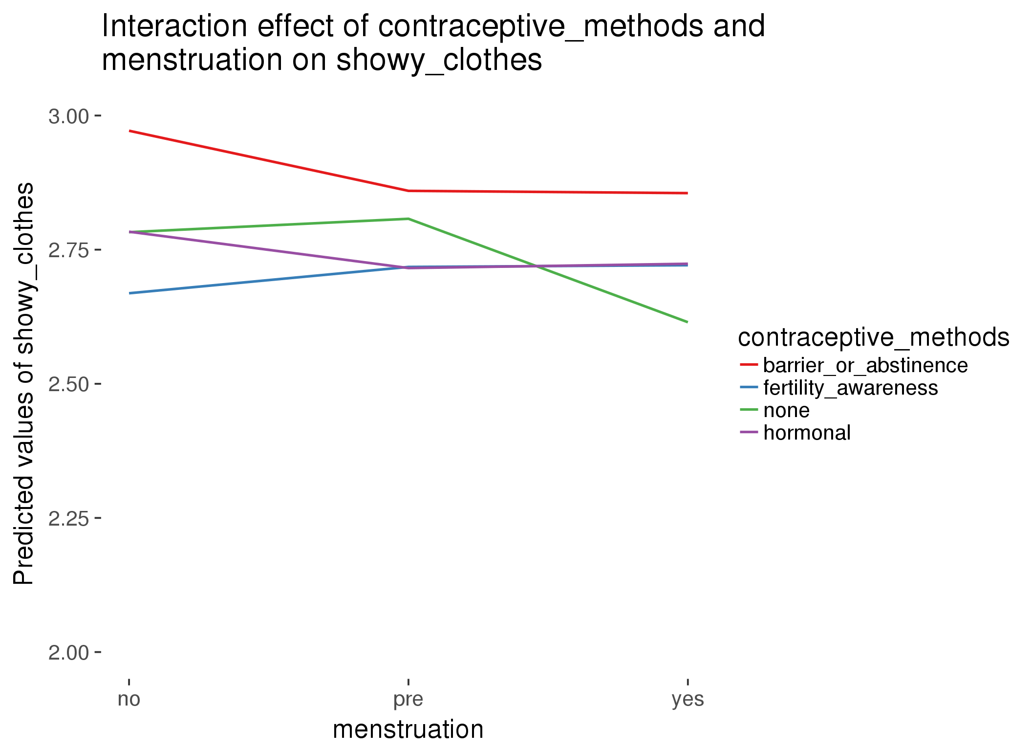
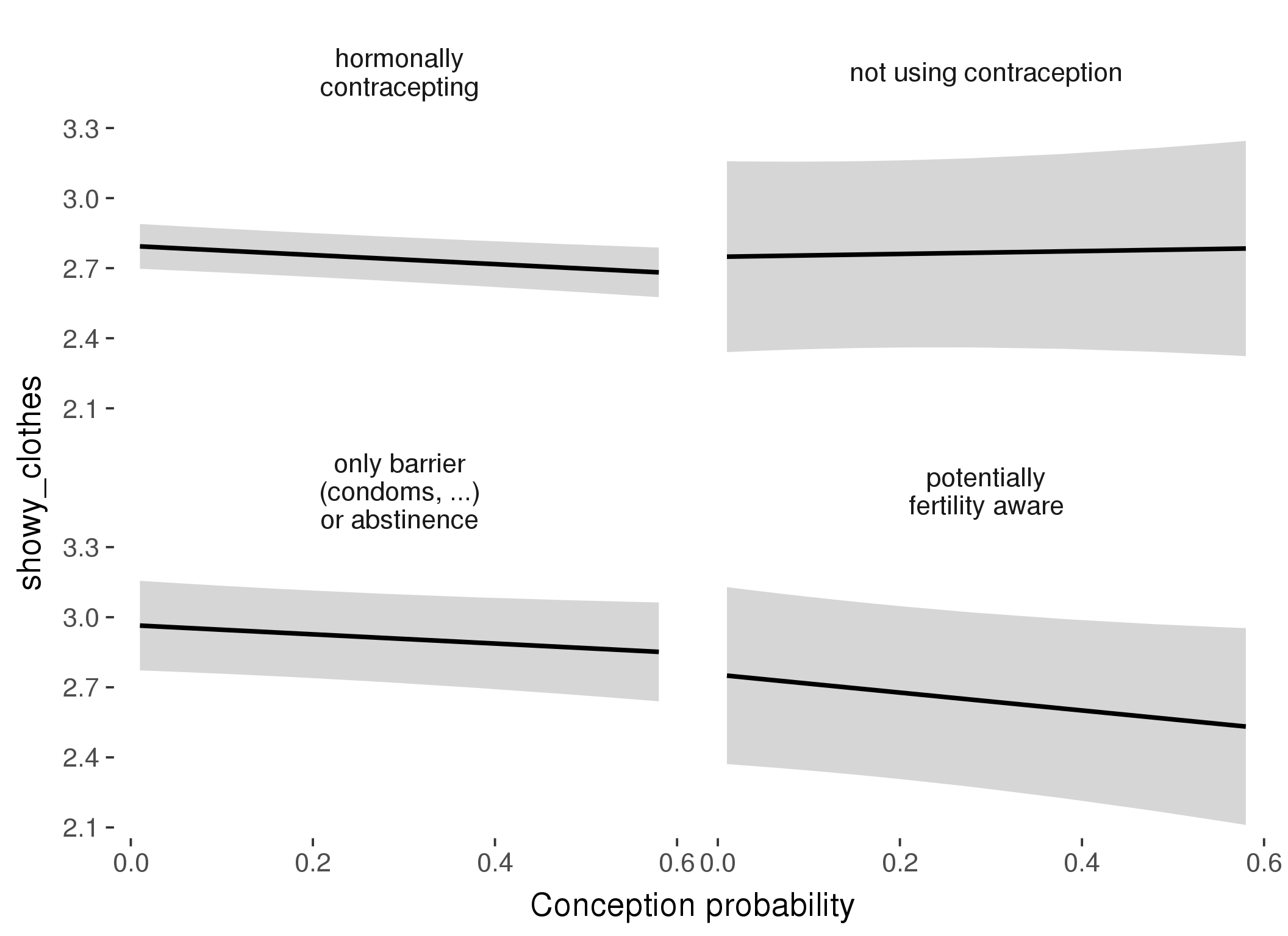
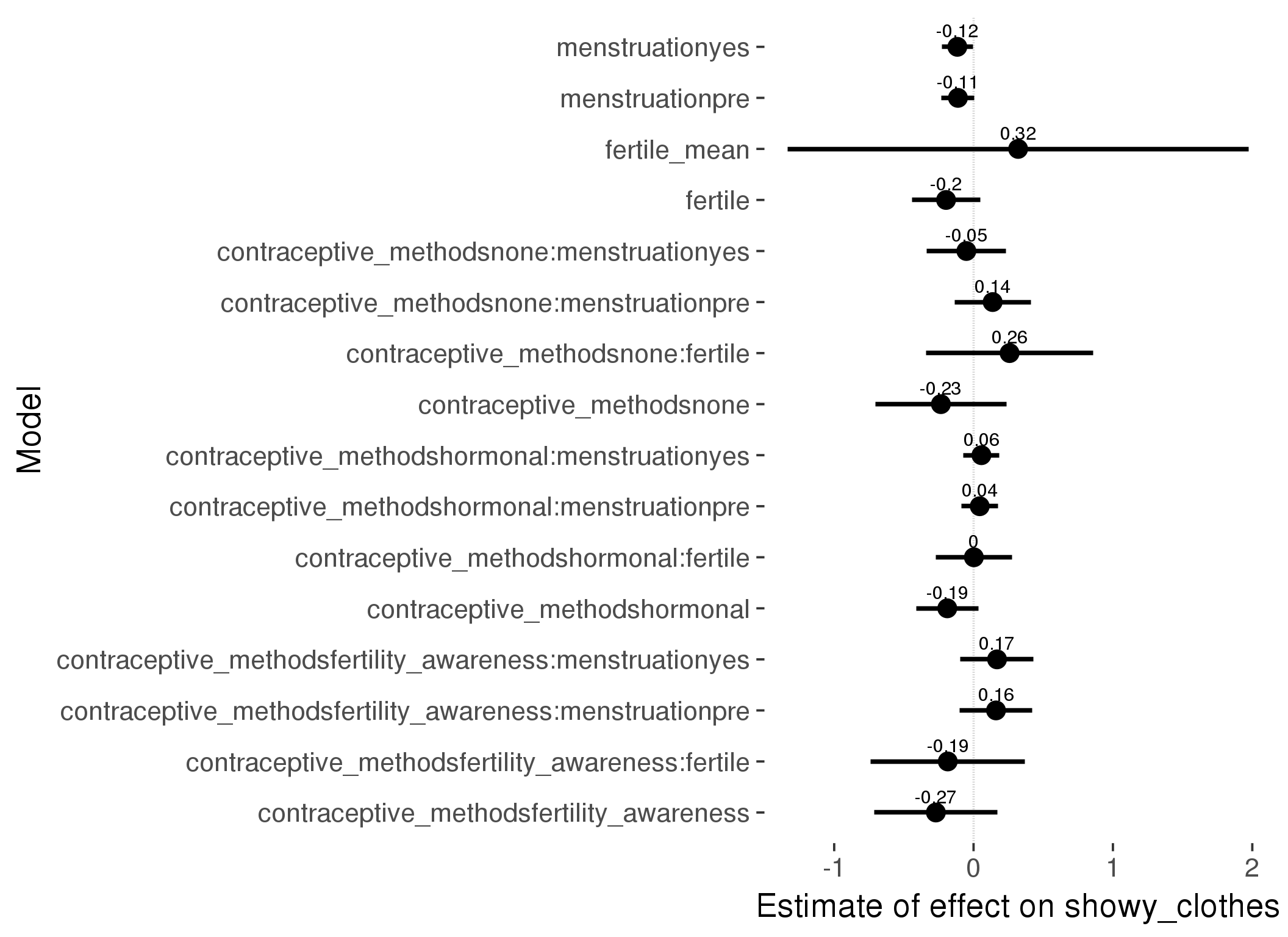
Linear mixed model fit by REML ['lmerMod']
Formula: showy_clothes ~ fertile_mean + (1 | person) + contraceptive_methods +
fertile + menstruation + fertile:contraceptive_methods + menstruation:contraceptive_methods
Data: diary
Subset: !is.na(included_lax) & contraceptive_method != "other"
REML criterion at convergence: 53710
Scaled residuals:
Min 1Q Median 3Q Max
-3.741 -0.636 -0.095 0.630 4.148
Random effects:
Groups Name Variance Std.Dev.
person (Intercept) 0.816 0.903
Residual 1.247 1.117
Number of obs: 17029, groups: person, 513
Fixed effects:
Estimate Std. Error t value
(Intercept) 2.95016 0.17369 16.99
fertile_mean 0.31980 0.84426 0.38
contraceptive_methodsfertility_awareness -0.27038 0.22597 -1.20
contraceptive_methodsnone -0.23437 0.23952 -0.98
contraceptive_methodshormonal -0.18856 0.11392 -1.66
fertile -0.19729 0.12460 -1.58
menstruationpre -0.11203 0.06018 -1.86
menstruationyes -0.11624 0.05748 -2.02
contraceptive_methodsfertility_awareness:fertile -0.18511 0.28297 -0.65
contraceptive_methodsnone:fertile 0.25855 0.30634 0.84
contraceptive_methodshormonal:fertile 0.00228 0.13918 0.02
contraceptive_methodsfertility_awareness:menstruationpre 0.16107 0.13330 1.21
contraceptive_methodsnone:menstruationpre 0.13697 0.13936 0.98
contraceptive_methodshormonal:menstruationpre 0.04427 0.06779 0.65
contraceptive_methodsfertility_awareness:menstruationyes 0.16848 0.13397 1.26
contraceptive_methodsnone:menstruationyes -0.05162 0.14573 -0.35
contraceptive_methodshormonal:menstruationyes 0.05648 0.06555 0.86
refitting model(s) with ML (instead of REML)
| Df | AIC | BIC | logLik | deviance | Chisq | Chi Df | Pr(>Chisq) | |
|---|---|---|---|---|---|---|---|---|
| add_main | 13 | 53698 | 53799 | -26836 | 53672 | NA | NA | NA |
| by_method | 19 | 53702 | 53849 | -26832 | 53664 | 7.97 | 6 | 0.2403 |
M_m2: Moderation by participant age
model %>%
test_moderator("age_group", diary, xlevels = 5)refitting model(s) with ML (instead of REML)
| Df | AIC | BIC | logLik | deviance | Chisq | Chi Df | Pr(>Chisq) | |
|---|---|---|---|---|---|---|---|---|
| with_main | 19 | 84628 | 84784 | -42295 | 84590 | NA | NA | NA |
| with_mod | 27 | 84625 | 84846 | -42285 | 84571 | 19.15 | 8 | 0.0141 |
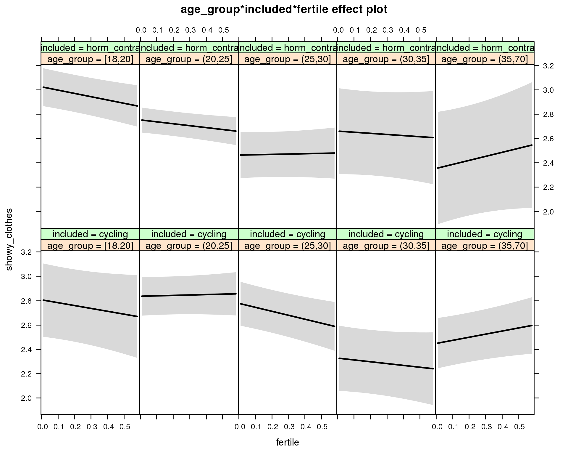
Linear mixed model fit by REML ['lmerMod']
Formula: showy_clothes ~ menstruation + fertile_mean + (1 | person) +
age_group + included + fertile + menstruation:included +
age_group:included + age_group:fertile + included:fertile + age_group:included:fertile
Data: diary
REML criterion at convergence: 84640
Scaled residuals:
Min 1Q Median 3Q Max
-3.715 -0.628 -0.102 0.623 4.119
Random effects:
Groups Name Variance Std.Dev.
person (Intercept) 0.787 0.887
Residual 1.258 1.122
Number of obs: 26685, groups: person, 1054
Fixed effects:
Estimate Std. Error t value
(Intercept) 2.7395 0.1630 16.81
menstruationpre -0.0696 0.0342 -2.03
menstruationyes -0.1162 0.0323 -3.60
fertile_mean 0.5760 0.3598 1.60
age_group(20,25] 0.0296 0.1742 0.17
age_group(25,30] -0.0290 0.1793 -0.16
age_group(30,35] -0.4789 0.2058 -2.33
age_group(35,70] -0.3582 0.1864 -1.92
includedhorm_contra 0.1996 0.1746 1.14
fertile -0.2355 0.1975 -1.19
menstruationpre:includedhorm_contra 0.0352 0.0440 0.80
menstruationyes:includedhorm_contra 0.0676 0.0423 1.60
age_group(20,25]:includedhorm_contra -0.3013 0.1987 -1.52
age_group(25,30]:includedhorm_contra -0.5317 0.2188 -2.43
age_group(30,35]:includedhorm_contra 0.1152 0.2849 0.40
age_group(35,70]:includedhorm_contra -0.3122 0.3113 -1.00
age_group(20,25]:fertile 0.2699 0.2188 1.23
age_group(25,30]:fertile -0.0899 0.2256 -0.40
age_group(30,35]:fertile 0.0851 0.2612 0.33
age_group(35,70]:fertile 0.4898 0.2357 2.08
includedhorm_contra:fertile -0.0348 0.2191 -0.16
age_group(20,25]:includedhorm_contra:fertile -0.1575 0.2451 -0.64
age_group(25,30]:includedhorm_contra:fertile 0.3883 0.2716 1.43
age_group(30,35]:includedhorm_contra:fertile 0.0930 0.3506 0.27
age_group(35,70]:includedhorm_contra:fertile 0.1113 0.3983 0.28
M_m3: Moderation by weekend
model %>%
test_moderator("weekend", diary, xlevels = 2) refitting model(s) with ML (instead of REML)
| Df | AIC | BIC | logLik | deviance | Chisq | Chi Df | Pr(>Chisq) | |
|---|---|---|---|---|---|---|---|---|
| with_main | 13 | 84648 | 84755 | -42311 | 84622 | NA | NA | NA |
| with_mod | 15 | 84652 | 84775 | -42311 | 84622 | 0.3505 | 2 | 0.8393 |
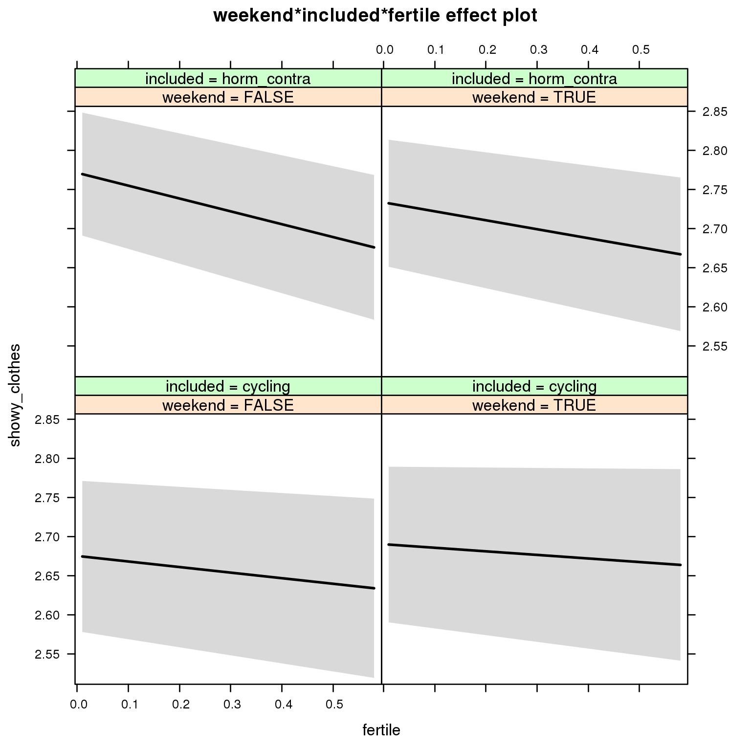
Linear mixed model fit by REML ['lmerMod']
Formula: showy_clothes ~ menstruation + fertile_mean + (1 | person) +
weekend + included + fertile + menstruation:included + weekend:included +
weekend:fertile + included:fertile + weekend:included:fertile
Data: diary
REML criterion at convergence: 84678
Scaled residuals:
Min 1Q Median 3Q Max
-3.729 -0.628 -0.104 0.624 4.123
Random effects:
Groups Name Variance Std.Dev.
person (Intercept) 0.811 0.90
Residual 1.259 1.12
Number of obs: 26685, groups: person, 1054
Fixed effects:
Estimate Std. Error t value
(Intercept) 2.6010 0.0799 32.5
menstruationpre -0.0689 0.0342 -2.0
menstruationyes -0.1135 0.0323 -3.5
fertile_mean 0.6112 0.3624 1.7
weekendTRUE 0.0150 0.0298 0.5
includedhorm_contra 0.0781 0.0665 1.2
fertile -0.0713 0.0841 -0.8
menstruationpre:includedhorm_contra 0.0372 0.0440 0.8
menstruationyes:includedhorm_contra 0.0667 0.0423 1.6
weekendTRUE:includedhorm_contra -0.0528 0.0384 -1.4
weekendTRUE:fertile 0.0256 0.1157 0.2
includedhorm_contra:fertile -0.0932 0.1068 -0.9
weekendTRUE:includedhorm_contra:fertile 0.0243 0.1472 0.2
M_m4: Moderation by weekday
model %>%
test_moderator("weekday", diary, xlevels = 7)refitting model(s) with ML (instead of REML)
| Df | AIC | BIC | logLik | deviance | Chisq | Chi Df | Pr(>Chisq) | |
|---|---|---|---|---|---|---|---|---|
| with_main | 23 | 84631 | 84819 | -42292 | 84585 | NA | NA | NA |
| with_mod | 35 | 84649 | 84936 | -42290 | 84579 | 5.842 | 12 | 0.9239 |
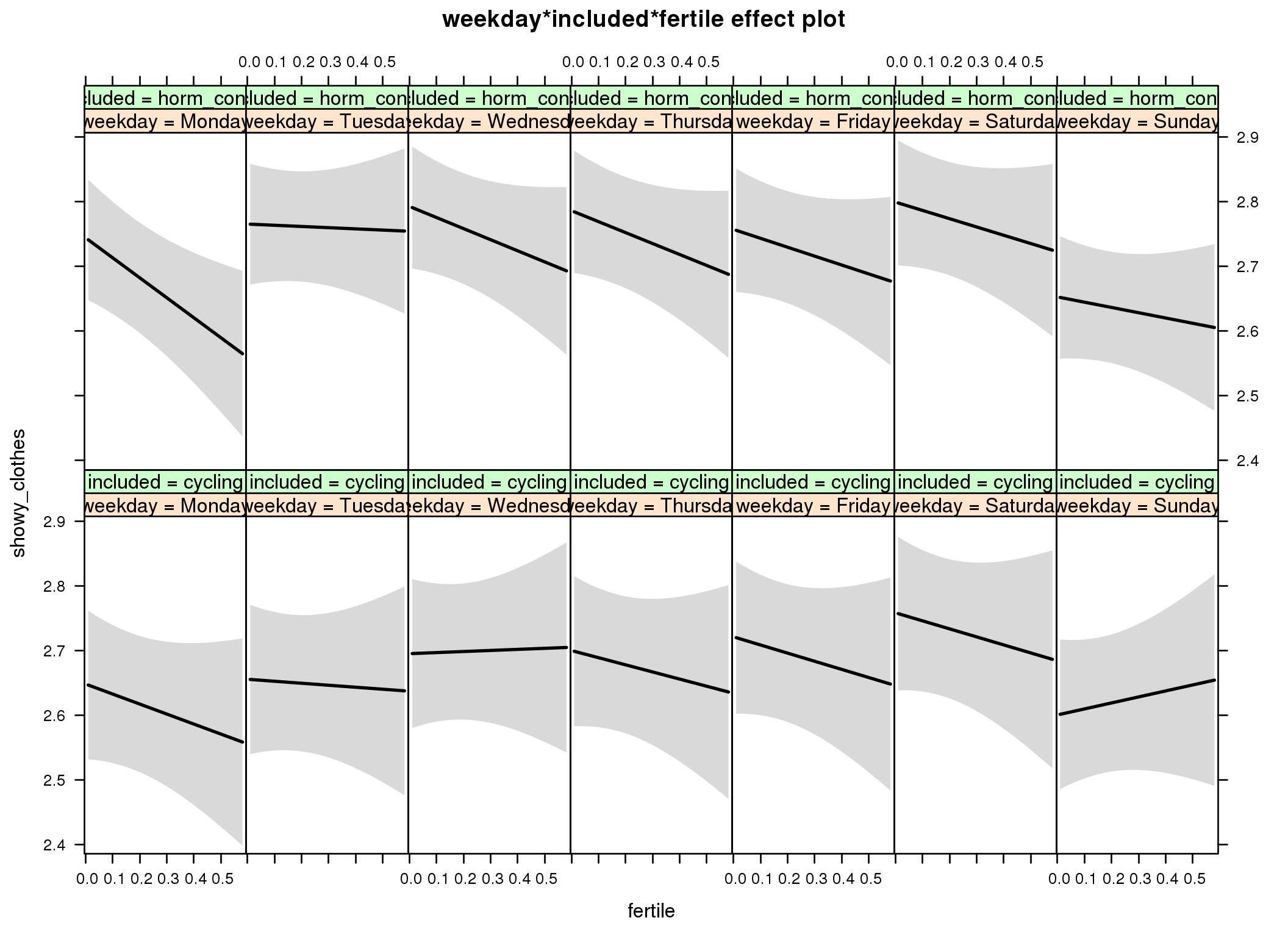
Linear mixed model fit by REML ['lmerMod']
Formula: showy_clothes ~ menstruation + fertile_mean + (1 | person) +
weekday + included + fertile + menstruation:included + weekday:included +
weekday:fertile + included:fertile + weekday:included:fertile
Data: diary
REML criterion at convergence: 84701
Scaled residuals:
Min 1Q Median 3Q Max
-3.742 -0.630 -0.102 0.625 4.136
Random effects:
Groups Name Variance Std.Dev.
person (Intercept) 0.811 0.901
Residual 1.257 1.121
Number of obs: 26685, groups: person, 1054
Fixed effects:
Estimate Std. Error t value
(Intercept) 2.57279 0.08631 29.81
menstruationpre -0.06829 0.03423 -2.00
menstruationyes -0.11324 0.03225 -3.51
fertile_mean 0.61552 0.36249 1.70
weekdayTuesday 0.00739 0.05338 0.14
weekdayWednesday 0.04699 0.05329 0.88
weekdayThursday 0.05176 0.05390 0.96
weekdayFriday 0.07298 0.05481 1.33
weekdaySaturday 0.11014 0.05536 1.99
weekdaySunday -0.04777 0.05350 -0.89
includedhorm_contra 0.07828 0.07847 1.00
fertile -0.15475 0.15035 -1.03
menstruationpre:includedhorm_contra 0.03588 0.04394 0.82
menstruationyes:includedhorm_contra 0.06598 0.04228 1.56
weekdayTuesday:includedhorm_contra 0.01381 0.06858 0.20
weekdayWednesday:includedhorm_contra 0.00143 0.06880 0.02
weekdayThursday:includedhorm_contra -0.00990 0.06946 -0.14
weekdayFriday:includedhorm_contra -0.06009 0.07041 -0.85
weekdaySaturday:includedhorm_contra -0.05501 0.07123 -0.77
weekdaySunday:includedhorm_contra -0.04371 0.06905 -0.63
weekdayTuesday:fertile 0.12389 0.20696 0.60
weekdayWednesday:fertile 0.17125 0.20793 0.82
weekdayThursday:fertile 0.04435 0.21090 0.21
weekdayFriday:fertile 0.02886 0.21127 0.14
weekdaySaturday:fertile 0.03068 0.21408 0.14
weekdaySunday:fertile 0.24754 0.20805 1.19
includedhorm_contra:fertile -0.15435 0.19230 -0.80
weekdayTuesday:includedhorm_contra:fertile 0.16663 0.26415 0.63
weekdayWednesday:includedhorm_contra:fertile -0.03378 0.26623 -0.13
weekdayThursday:includedhorm_contra:fertile 0.09523 0.26837 0.35
weekdayFriday:includedhorm_contra:fertile 0.14260 0.26921 0.53
weekdaySaturday:includedhorm_contra:fertile 0.15032 0.27310 0.55
weekdaySunday:includedhorm_contra:fertile -0.02004 0.26575 -0.08
M_m5: Moderation by exclusion threshold
model %>%
test_moderator("included_levels", diary, xlevels = 4)refitting model(s) with ML (instead of REML)
| Df | AIC | BIC | logLik | deviance | Chisq | Chi Df | Pr(>Chisq) | |
|---|---|---|---|---|---|---|---|---|
| with_main | 17 | 84647 | 84786 | -42306 | 84613 | NA | NA | NA |
| with_mod | 23 | 84650 | 84838 | -42302 | 84604 | 9.232 | 6 | 0.1609 |
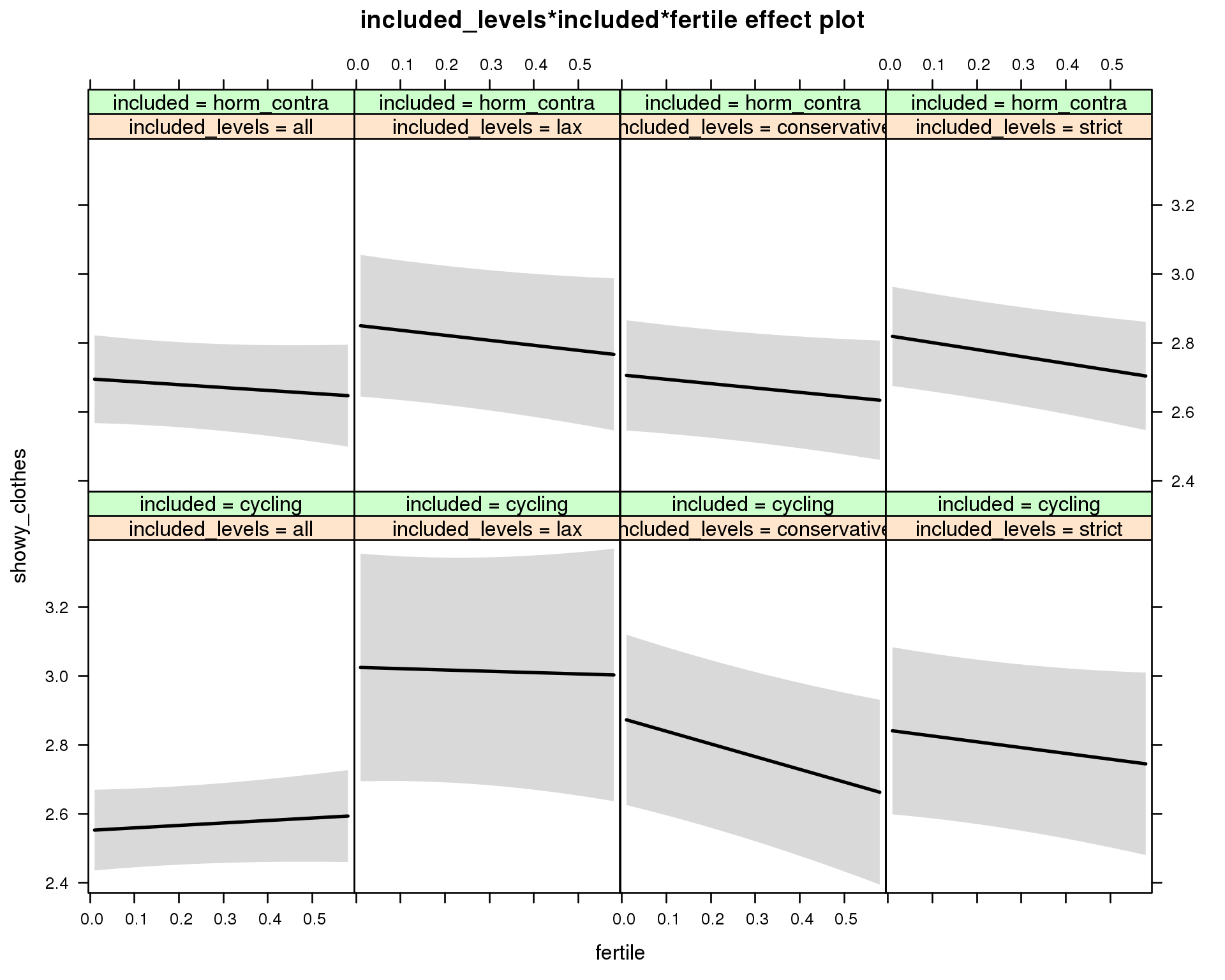
Linear mixed model fit by REML ['lmerMod']
Formula: showy_clothes ~ menstruation + fertile_mean + (1 | person) +
included_levels + included + fertile + menstruation:included +
included_levels:included + included_levels:fertile + included:fertile +
included_levels:included:fertile
Data: diary
REML criterion at convergence: 84669
Scaled residuals:
Min 1Q Median 3Q Max
-3.712 -0.627 -0.103 0.621 4.107
Random effects:
Groups Name Variance Std.Dev.
person (Intercept) 0.805 0.897
Residual 1.258 1.122
Number of obs: 26685, groups: person, 1054
Fixed effects:
Estimate Std. Error t value
(Intercept) 2.4842 0.0875 28.41
menstruationpre -0.0741 0.0343 -2.16
menstruationyes -0.1158 0.0323 -3.59
fertile_mean 0.5829 0.3648 1.60
included_levelslax 0.4731 0.1790 2.64
included_levelsconservative 0.3243 0.1397 2.32
included_levelsstrict 0.2906 0.1374 2.11
includedhorm_contra 0.1251 0.0903 1.39
fertile 0.0714 0.0873 0.82
menstruationpre:includedhorm_contra 0.0408 0.0440 0.93
menstruationyes:includedhorm_contra 0.0683 0.0423 1.61
included_levelslax:includedhorm_contra -0.3173 0.2179 -1.46
included_levelsconservative:includedhorm_contra -0.3129 0.1745 -1.79
included_levelsstrict:includedhorm_contra -0.1651 0.1689 -0.98
included_levelslax:fertile -0.1096 0.2133 -0.51
included_levelsconservative:fertile -0.4398 0.1593 -2.76
included_levelsstrict:fertile -0.2397 0.1594 -1.50
includedhorm_contra:fertile -0.1551 0.1333 -1.16
included_levelslax:includedhorm_contra:fertile 0.0475 0.2602 0.18
included_levelsconservative:includedhorm_contra:fertile 0.3972 0.2071 1.92
included_levelsstrict:includedhorm_contra:fertile 0.1218 0.2039 0.60
M_m6: Moderation by cycle length
model %>%
test_moderator("cycle_length_groups", diary, xlevels = 4)refitting model(s) with ML (instead of REML)
| Df | AIC | BIC | logLik | deviance | Chisq | Chi Df | Pr(>Chisq) | |
|---|---|---|---|---|---|---|---|---|
| with_main | 17 | 84655 | 84795 | -42311 | 84621 | NA | NA | NA |
| with_mod | 23 | 84664 | 84852 | -42309 | 84618 | 3.769 | 6 | 0.7079 |
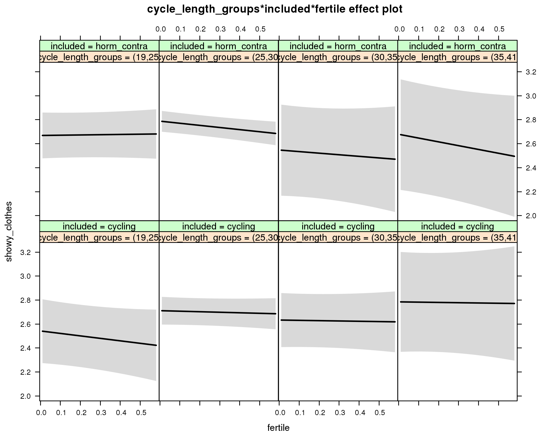
Linear mixed model fit by REML ['lmerMod']
Formula: showy_clothes ~ menstruation + fertile_mean + (1 | person) +
cycle_length_groups + included + fertile + menstruation:included +
cycle_length_groups:included + cycle_length_groups:fertile +
included:fertile + cycle_length_groups:included:fertile
Data: diary
REML criterion at convergence: 84675
Scaled residuals:
Min 1Q Median 3Q Max
-3.719 -0.629 -0.104 0.623 4.118
Random effects:
Groups Name Variance Std.Dev.
person (Intercept) 0.812 0.901
Residual 1.259 1.122
Number of obs: 26685, groups: person, 1054
Fixed effects:
Estimate Std. Error t value
(Intercept) 2.4713 0.1510 16.37
menstruationpre -0.0676 0.0343 -1.97
menstruationyes -0.1097 0.0325 -3.38
fertile_mean 0.5892 0.3672 1.60
cycle_length_groups(25,30] 0.1692 0.1483 1.14
cycle_length_groups(30,35] 0.0910 0.1783 0.51
cycle_length_groups(35,41] 0.2425 0.2527 0.96
includedhorm_contra 0.1094 0.1685 0.65
fertile -0.2062 0.1824 -1.13
menstruationpre:includedhorm_contra 0.0352 0.0440 0.80
menstruationyes:includedhorm_contra 0.0599 0.0425 1.41
cycle_length_groups(25,30]:includedhorm_contra -0.0496 0.1830 -0.27
cycle_length_groups(30,35]:includedhorm_contra -0.2123 0.2807 -0.76
cycle_length_groups(35,41]:includedhorm_contra -0.2327 0.3585 -0.65
cycle_length_groups(25,30]:fertile 0.1621 0.1957 0.83
cycle_length_groups(30,35]:fertile 0.1805 0.2317 0.78
cycle_length_groups(35,41]:fertile 0.1829 0.3273 0.56
includedhorm_contra:fertile 0.2276 0.2153 1.06
cycle_length_groups(25,30]:includedhorm_contra:fertile -0.3605 0.2318 -1.55
cycle_length_groups(30,35]:includedhorm_contra:fertile -0.3338 0.3648 -0.91
cycle_length_groups(35,41]:includedhorm_contra:fertile -0.5204 0.4309 -1.21
M_m7: Moderation by certainty about menstruation parameters
model %>%
test_moderator("certainty_menstruation", diary)refitting model(s) with ML (instead of REML)
| Df | AIC | BIC | logLik | deviance | Chisq | Chi Df | Pr(>Chisq) | |
|---|---|---|---|---|---|---|---|---|
| with_main | 13 | 84649 | 84755 | -42311 | 84623 | NA | NA | NA |
| with_mod | 15 | 84649 | 84772 | -42310 | 84619 | 3.725 | 2 | 0.1552 |
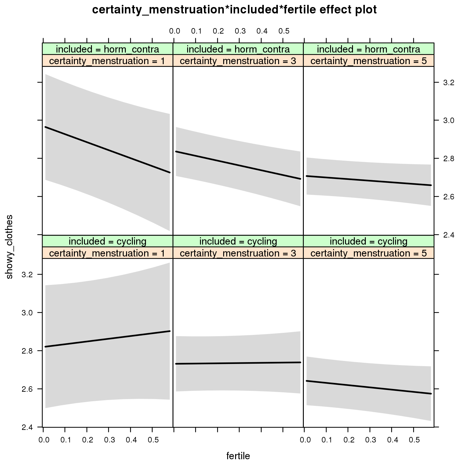
Linear mixed model fit by REML ['lmerMod']
Formula: showy_clothes ~ menstruation + fertile_mean + (1 | person) +
certainty_menstruation + included + fertile + menstruation:included +
certainty_menstruation:included + certainty_menstruation:fertile +
included:fertile + certainty_menstruation:included:fertile
Data: diary
REML criterion at convergence: 84674
Scaled residuals:
Min 1Q Median 3Q Max
-3.709 -0.626 -0.102 0.623 4.116
Random effects:
Groups Name Variance Std.Dev.
person (Intercept) 0.81 0.90
Residual 1.26 1.12
Number of obs: 26685, groups: person, 1054
Fixed effects:
Estimate Std. Error t value
(Intercept) 2.7844 0.2216 12.57
menstruationpre -0.0701 0.0343 -2.05
menstruationyes -0.1152 0.0323 -3.57
fertile_mean 0.6432 0.3630 1.77
certainty_menstruation -0.0442 0.0505 -0.87
includedhorm_contra 0.1517 0.2813 0.54
fertile 0.2086 0.2720 0.77
menstruationpre:includedhorm_contra 0.0382 0.0440 0.87
menstruationyes:includedhorm_contra 0.0703 0.0423 1.66
certainty_menstruation:includedhorm_contra -0.0210 0.0655 -0.32
certainty_menstruation:fertile -0.0653 0.0637 -1.02
includedhorm_contra:fertile -0.7114 0.3535 -2.01
certainty_menstruation:includedhorm_contra:fertile 0.1489 0.0817 1.82
M_m8: Moderation by cycle regularity
model %>%
test_moderator("cycle_regularity", diary)refitting model(s) with ML (instead of REML)
| Df | AIC | BIC | logLik | deviance | Chisq | Chi Df | Pr(>Chisq) | |
|---|---|---|---|---|---|---|---|---|
| with_main | 15 | 84655 | 84778 | -42312 | 84625 | NA | NA | NA |
| with_mod | 19 | 84659 | 84815 | -42311 | 84621 | 3.588 | 4 | 0.4647 |
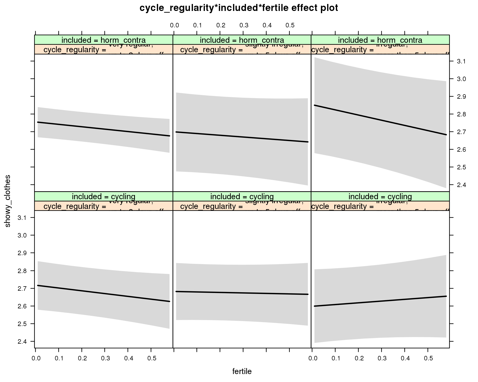
Linear mixed model fit by REML ['lmerMod']
Formula: showy_clothes ~ menstruation + fertile_mean + (1 | person) +
cycle_regularity + included + fertile + menstruation:included +
cycle_regularity:included + cycle_regularity:fertile + included:fertile +
cycle_regularity:included:fertile
Data: diary
REML criterion at convergence: 84677
Scaled residuals:
Min 1Q Median 3Q Max
-3.716 -0.628 -0.105 0.622 4.123
Random effects:
Groups Name Variance Std.Dev.
person (Intercept) 0.814 0.902
Residual 1.259 1.122
Number of obs: 26685, groups: person, 1054
Fixed effects:
Estimate Std. Error t value
(Intercept) 2.6457 0.0933 28.35
menstruationpre -0.0711 0.0343 -2.07
menstruationyes -0.1149 0.0323 -3.56
fertile_mean 0.6008 0.3646 1.65
cycle_regularityslightly irregular,\nup to 5 days off -0.0355 0.1081 -0.33
cycle_regularityirregular,\nmore than 5 days off -0.1194 0.1272 -0.94
includedhorm_contra 0.0185 0.0849 0.22
fertile -0.1584 0.0957 -1.66
menstruationpre:includedhorm_contra 0.0398 0.0440 0.90
menstruationyes:includedhorm_contra 0.0696 0.0423 1.64
cycle_regularityslightly irregular,\nup to 5 days off:includedhorm_contra -0.0203 0.1633 -0.12
cycle_regularityirregular,\nmore than 5 days off:includedhorm_contra 0.2170 0.1931 1.12
cycle_regularityslightly irregular,\nup to 5 days off:fertile 0.1308 0.1320 0.99
cycle_regularityirregular,\nmore than 5 days off:fertile 0.2567 0.1623 1.58
includedhorm_contra:fertile 0.0225 0.1121 0.20
cycle_regularityslightly irregular,\nup to 5 days off:includedhorm_contra:fertile -0.0933 0.1960 -0.48
cycle_regularityirregular,\nmore than 5 days off:includedhorm_contra:fertile -0.4137 0.2420 -1.71
M_m9: Moderation by cohabitation status
model %>%
test_moderator("cohabitation", diary)refitting model(s) with ML (instead of REML)
| Df | AIC | BIC | logLik | deviance | Chisq | Chi Df | Pr(>Chisq) | |
|---|---|---|---|---|---|---|---|---|
| with_main | 15 | 84646 | 84769 | -42308 | 84616 | NA | NA | NA |
| with_mod | 19 | 84651 | 84807 | -42307 | 84613 | 2.62 | 4 | 0.6233 |
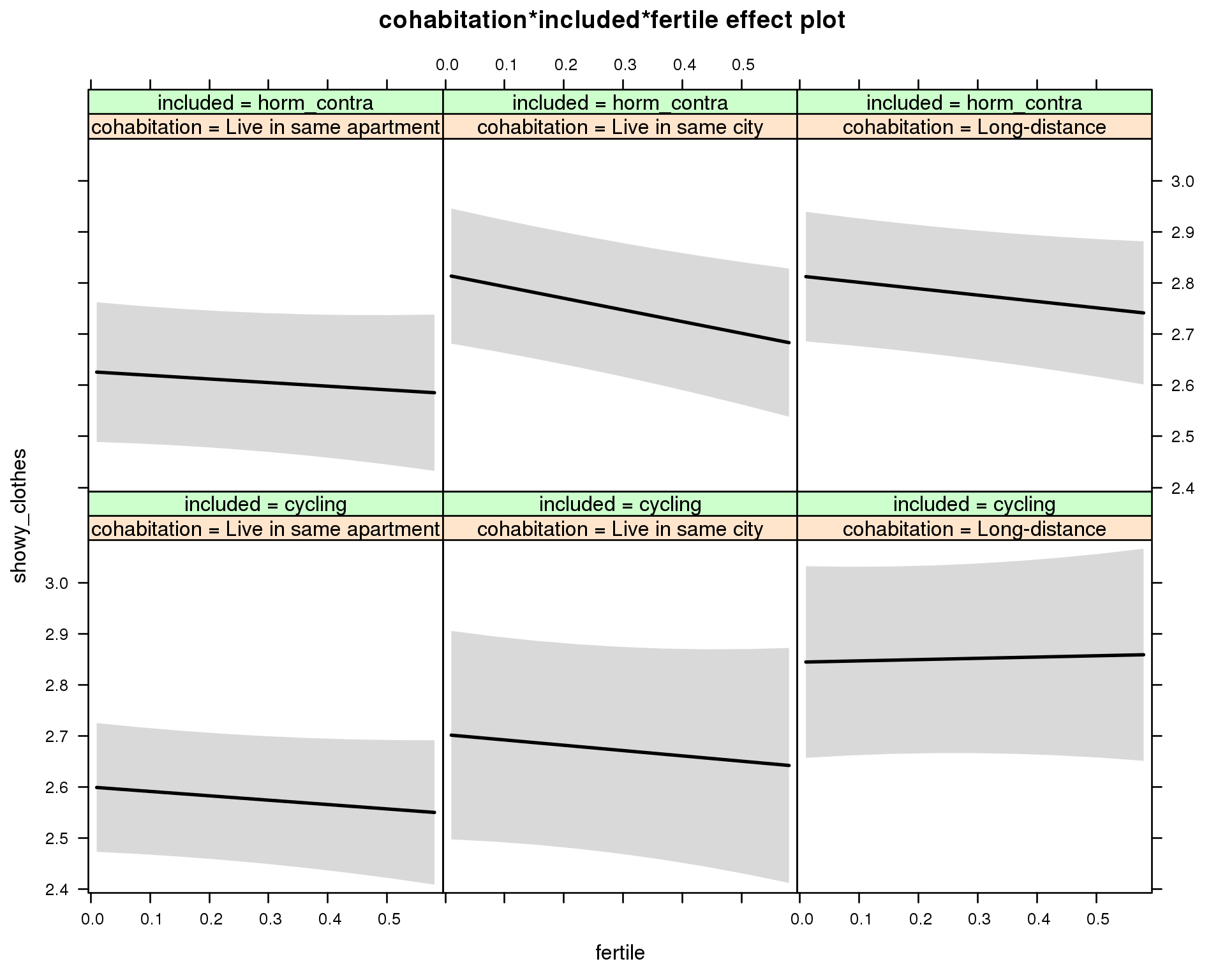
Linear mixed model fit by REML ['lmerMod']
Formula: showy_clothes ~ menstruation + fertile_mean + (1 | person) +
cohabitation + included + fertile + menstruation:included +
cohabitation:included + cohabitation:fertile + included:fertile + cohabitation:included:fertile
Data: diary
REML criterion at convergence: 84672
Scaled residuals:
Min 1Q Median 3Q Max
-3.728 -0.628 -0.105 0.626 4.118
Random effects:
Groups Name Variance Std.Dev.
person (Intercept) 0.806 0.898
Residual 1.259 1.122
Number of obs: 26685, groups: person, 1054
Fixed effects:
Estimate Std. Error t value
(Intercept) 2.5284 0.0901 28.06
menstruationpre -0.0694 0.0342 -2.03
menstruationyes -0.1143 0.0323 -3.54
fertile_mean 0.5971 0.3624 1.65
cohabitationLive in same city 0.1026 0.1223 0.84
cohabitationLong-distance 0.2444 0.1152 2.12
includedhorm_contra 0.0084 0.0968 0.09
fertile -0.0856 0.0864 -0.99
menstruationpre:includedhorm_contra 0.0364 0.0440 0.83
menstruationyes:includedhorm_contra 0.0671 0.0423 1.59
cohabitationLive in same city:includedhorm_contra 0.0869 0.1562 0.56
cohabitationLong-distance:includedhorm_contra -0.0570 0.1495 -0.38
cohabitationLive in same city:fertile -0.0184 0.1578 -0.12
cohabitationLong-distance:fertile 0.1106 0.1421 0.78
includedhorm_contra:fertile 0.0149 0.1262 0.12
cohabitationLive in same city:includedhorm_contra:fertile -0.1393 0.1973 -0.71
cohabitationLong-distance:includedhorm_contra:fertile -0.1643 0.1831 -0.90
M_m10: Moderation by relationship status
model %>%
test_moderator("relationship_status_clean", diary)refitting model(s) with ML (instead of REML)
| Df | AIC | BIC | logLik | deviance | Chisq | Chi Df | Pr(>Chisq) | |
|---|---|---|---|---|---|---|---|---|
| with_main | 15 | 84649 | 84772 | -42309 | 84619 | NA | NA | NA |
| with_mod | 19 | 84651 | 84806 | -42306 | 84613 | 6.093 | 4 | 0.1923 |
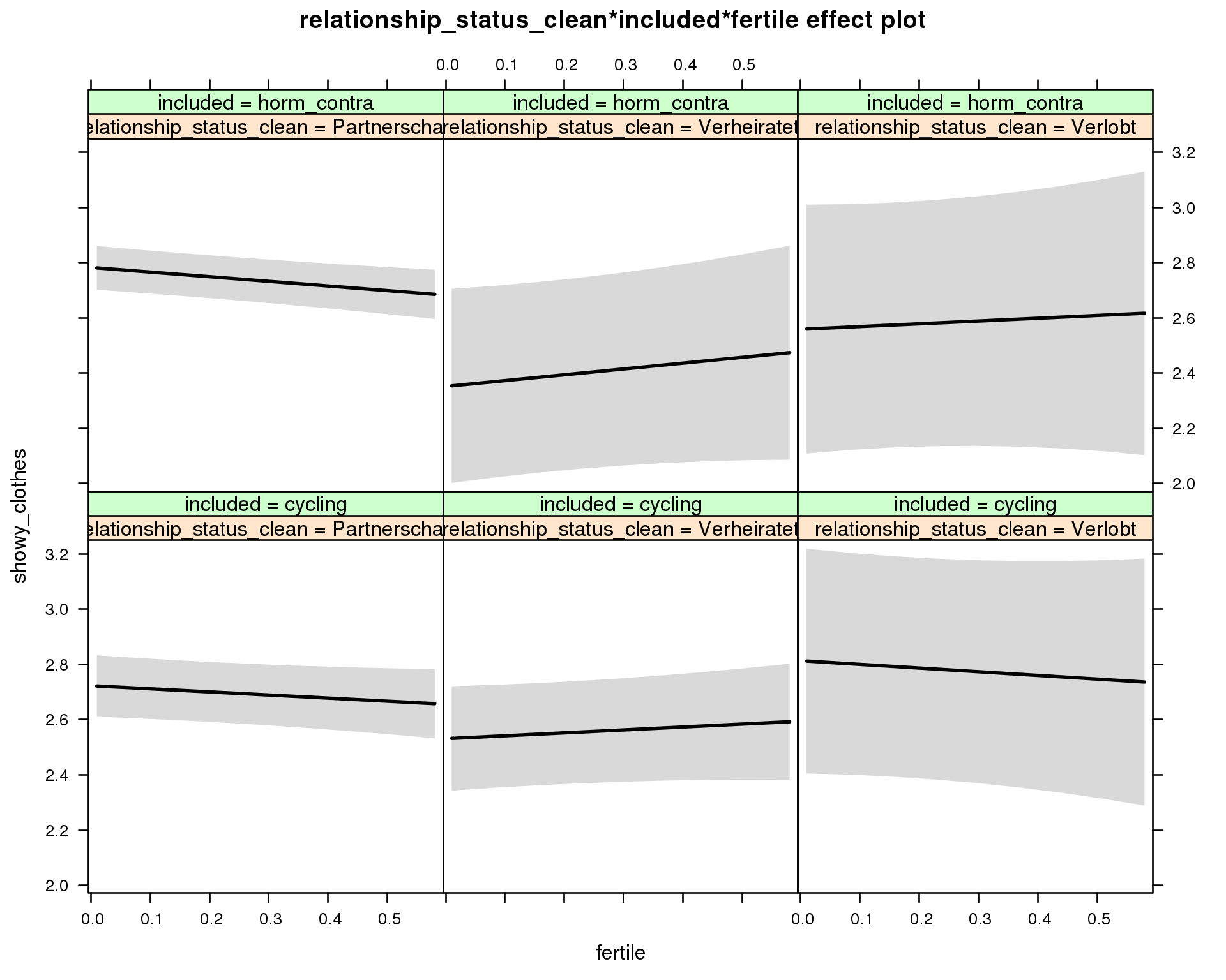
Linear mixed model fit by REML ['lmerMod']
Formula: showy_clothes ~ menstruation + fertile_mean + (1 | person) +
relationship_status_clean + included + fertile + menstruation:included +
relationship_status_clean:included + relationship_status_clean:fertile +
included:fertile + relationship_status_clean:included:fertile
Data: diary
REML criterion at convergence: 84662
Scaled residuals:
Min 1Q Median 3Q Max
-3.720 -0.629 -0.105 0.624 4.113
Random effects:
Groups Name Variance Std.Dev.
person (Intercept) 0.809 0.899
Residual 1.258 1.122
Number of obs: 26685, groups: person, 1054
Fixed effects:
Estimate Std. Error t value
(Intercept) 2.6523 0.0844 31.41
menstruationpre -0.0693 0.0342 -2.02
menstruationyes -0.1135 0.0323 -3.52
fertile_mean 0.5914 0.3625 1.63
relationship_status_cleanVerheiratet -0.1919 0.1119 -1.72
relationship_status_cleanVerlobt 0.0906 0.2158 0.42
includedhorm_contra 0.0418 0.0724 0.58
fertile -0.1121 0.0791 -1.42
menstruationpre:includedhorm_contra 0.0367 0.0440 0.83
menstruationyes:includedhorm_contra 0.0670 0.0423 1.58
relationship_status_cleanVerheiratet:includedhorm_contra -0.2391 0.2156 -1.11
relationship_status_cleanVerlobt:includedhorm_contra -0.3148 0.3184 -0.99
relationship_status_cleanVerheiratet:fertile 0.2180 0.1393 1.57
relationship_status_cleanVerlobt:fertile -0.0211 0.2612 -0.08
includedhorm_contra:fertile -0.0558 0.0964 -0.58
relationship_status_cleanVerheiratet:includedhorm_contra:fertile 0.1606 0.2623 0.61
relationship_status_cleanVerlobt:includedhorm_contra:fertile 0.2895 0.4057 0.71
Male attention
model_summaries$male_attention_1Model summary
Model summary
model %>%
print_summary()Linear mixed model fit by REML
t-tests use Satterthwaite approximations to degrees of freedom ['lmerMod']
Formula: male_attention_1 ~ included * (menstruation + fertile) + fertile_mean + (1 | person)
Data: diary
REML criterion at convergence: 101959
Scaled residuals:
Min 1Q Median 3Q Max
-2.8750 -0.7325 -0.0031 0.7181 2.8683
Random effects:
Groups Name Variance Std.Dev.
person (Intercept) 0.998 0.999
Residual 2.447 1.564
Number of obs: 26680, groups: person, 1054
Fixed effects:
Estimate Std. Error df t value Pr(>|t|)
(Intercept) 3.50617 0.09293 1502.00000 37.73 < 2e-16 ***
includedhorm_contra 0.20538 0.07600 1516.00000 2.70 0.00696 **
menstruationpre -0.05212 0.04765 26112.00000 -1.09 0.27407
menstruationyes -0.17163 0.04487 26239.00000 -3.83 0.00013 ***
fertile 0.07233 0.09617 26077.00000 0.75 0.45203
fertile_mean 0.00521 0.42921 1612.00000 0.01 0.99032
includedhorm_contra:menstruationpre -0.04231 0.06118 26110.00000 -0.69 0.48914
includedhorm_contra:menstruationyes -0.00160 0.05883 26212.00000 -0.03 0.97837
includedhorm_contra:fertile -0.35889 0.12175 26233.00000 -2.95 0.00320 **
---
Signif. codes: 0 '***' 0.001 '**' 0.01 '*' 0.05 '.' 0.1 ' ' 1
Correlation of Fixed Effects:
(Intr) incld_ mnstrtnp mnstrtny fertil frtl_m inclddhrm_cntr:mnstrtnp
inclddhrm_c -0.474
menstrutnpr -0.200 0.251
menstrutnys -0.194 0.241 0.396
fertile -0.191 0.310 0.466 0.384
fertile_men -0.771 -0.028 -0.007 -0.005 -0.079
inclddhrm_cntr:mnstrtnp 0.164 -0.315 -0.779 -0.308 -0.362 -0.006
inclddhrm_cntr:mnstrtny 0.155 -0.296 -0.302 -0.763 -0.292 -0.006 0.381
inclddhrm_cntr:f 0.190 -0.391 -0.368 -0.303 -0.786 0.011 0.466
inclddhrm_cntr:mnstrtny
inclddhrm_c
menstrutnpr
menstrutnys
fertile
fertile_men
inclddhrm_cntr:mnstrtnp
inclddhrm_cntr:mnstrtny
inclddhrm_cntr:f 0.380
Effect size standardised by residual variance (\(\frac{b}{ SD_{residual} }\)): 0.05 [-0.07;0.17].
Marginal effect plots
model %>%
plot_all_effects()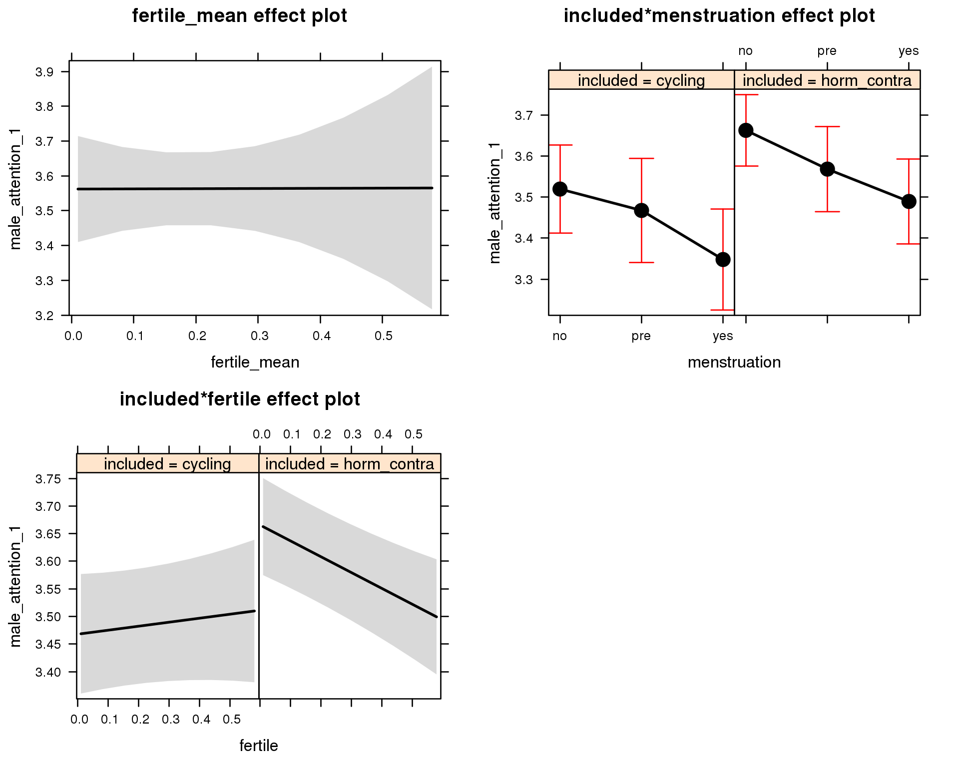
Outcome distribution
model %>%
plot_outcome(diary) + xlab(outcome_label)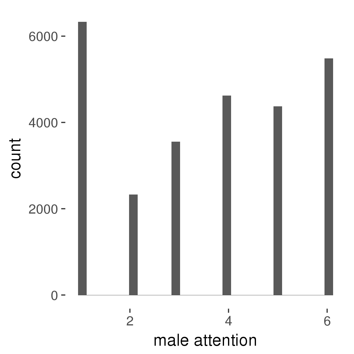
Diagnostics
model %>%
print_diagnostics()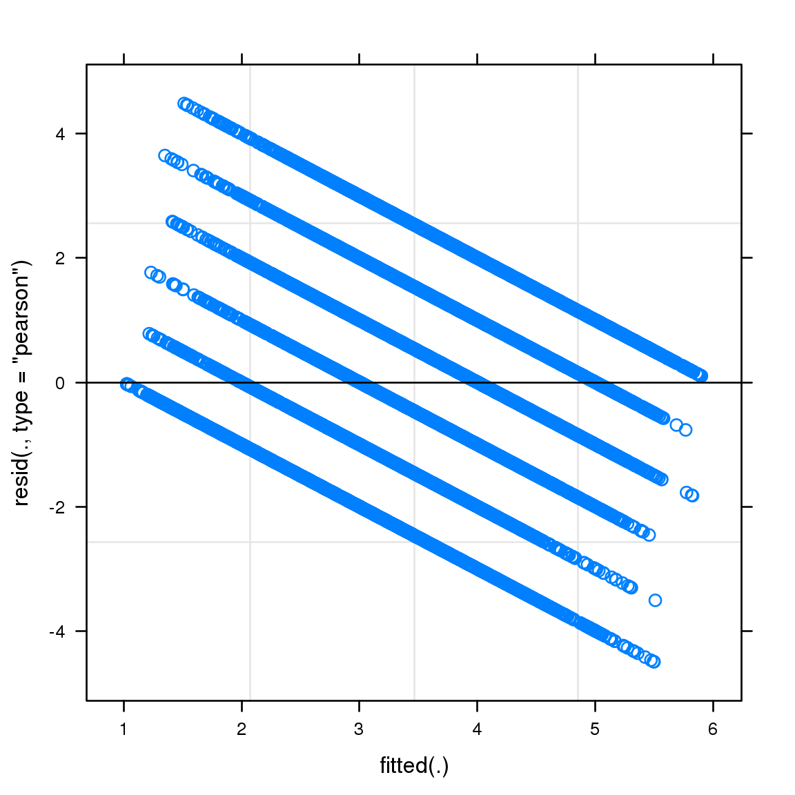
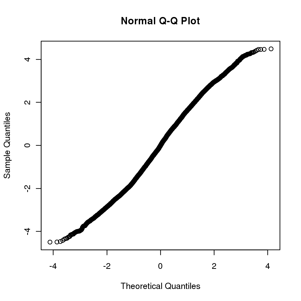
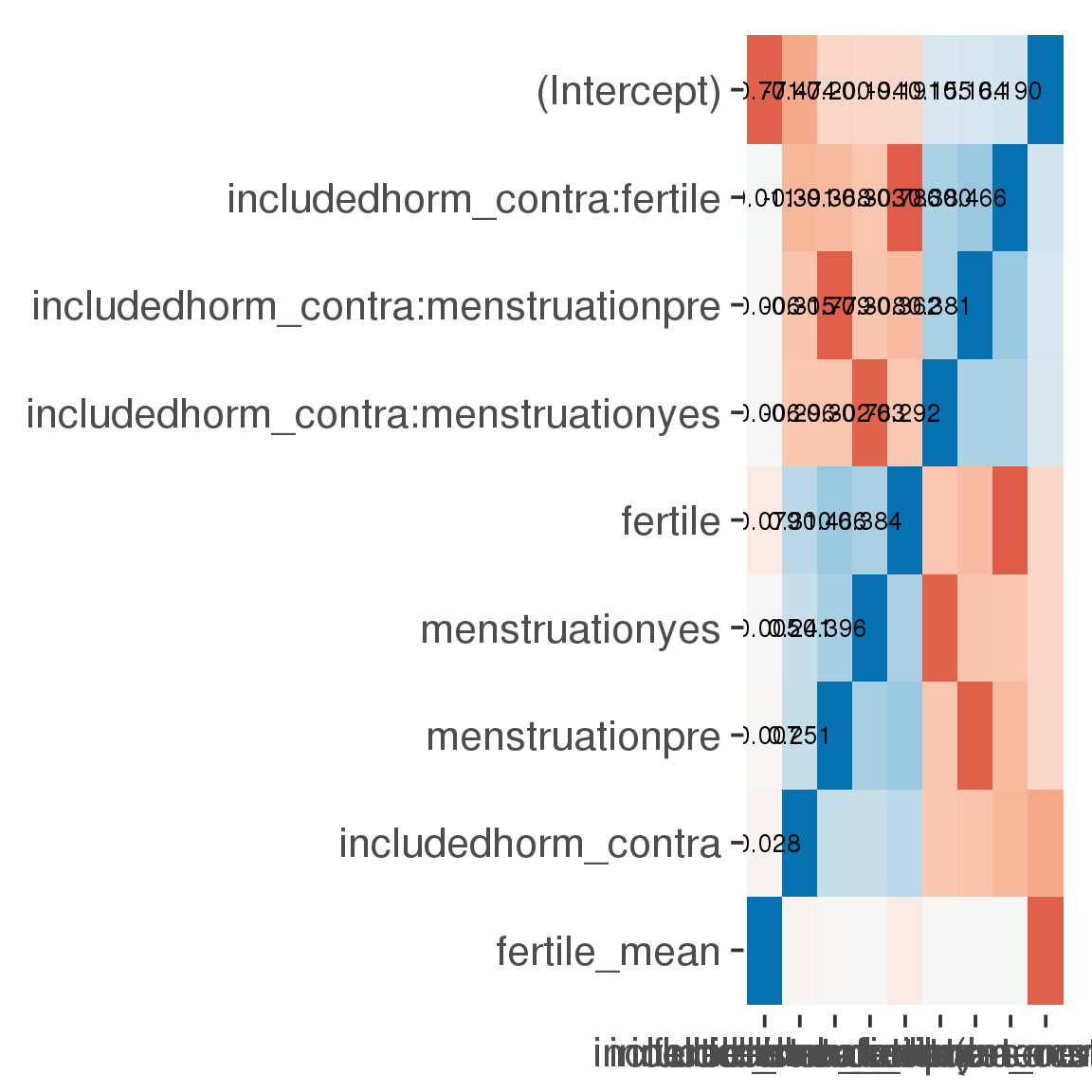
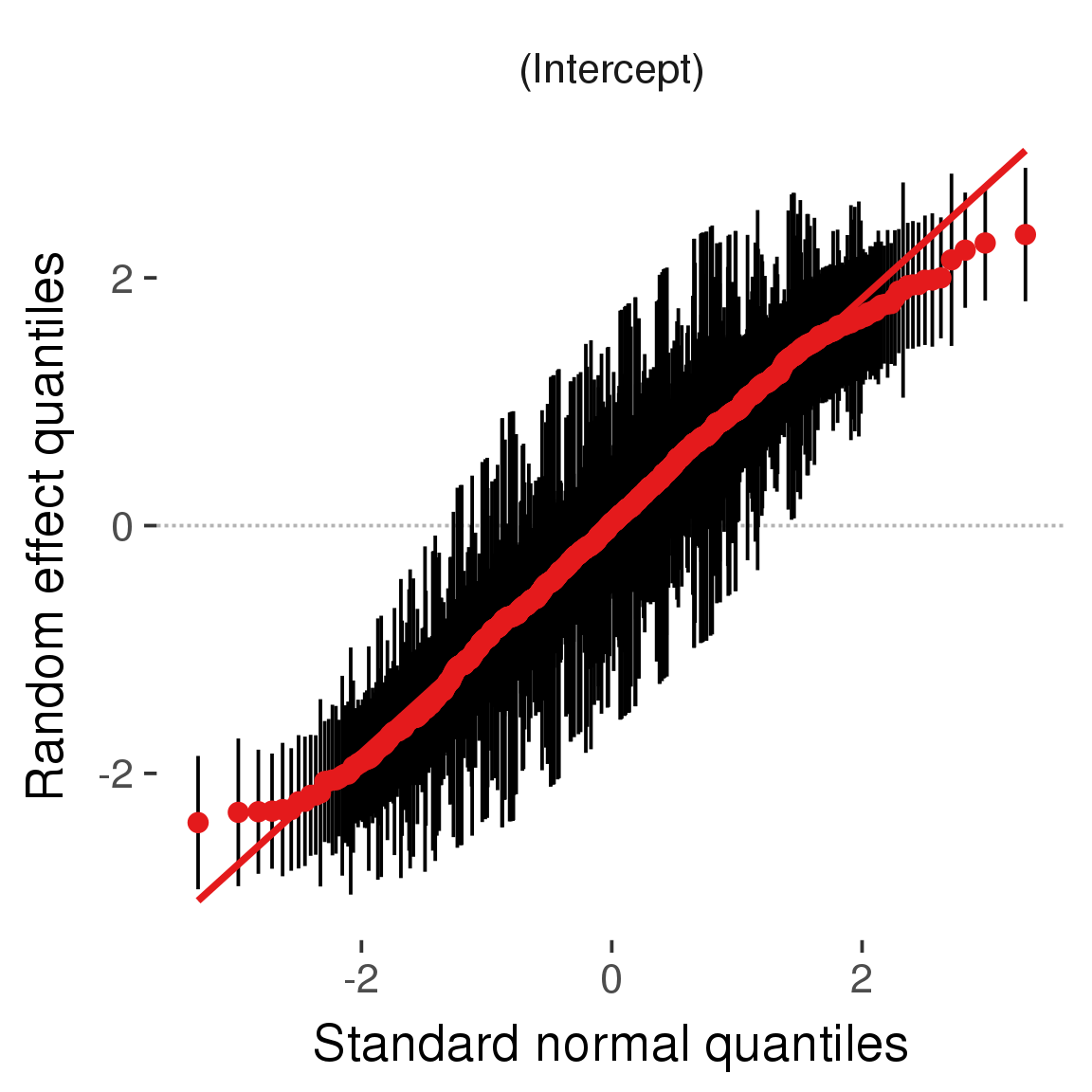
Curves
Here, we continuously plot the outcome over the course of the cycle. Because cycle lengths vary, we subset the data to cycles in a certain range. If the red curve traces the pink curve, our predictor accurately maps the relationship between fertile window probability and the outcome.
Cycle lengths from 21 to 36
Backward-counted
model %>%
plot_curve(diary %>% filter(minimum_cycle_length_diary <= 36, minimum_cycle_length_diary > 20) %>% mutate(fertile=prc_stirn_b))outcome = names(model@frame)[1]
outcome_label = recode(str_replace_all(str_replace_all(str_replace_all(outcome, "_", " "), " pair", "-pair"), " 1", ""),
"desirability 1" = "self-perceived desirability",
"NARQ admiration" = "narcissistic admiration",
"NARQ rivalry" = "narcissistic rivalry",
"extra-pair" = "extra-pair desire & behaviour",
"had sexual intercourse" = "sexual intercourse")
library(ggplot2)
# form a subset and run the model without the hormonal contraception and the fertility predictors
tmp = diary %>%
filter(!is.na(fertile), !is.na(included),
RCD > -1 * minimum_cycle_length_diary, RCD > -40)
new_form = update.formula(formula(model), new = . ~ . - fertile * included)
tmp$residuals = residuals(update(model, new_form, data = tmp , na.action = na.exclude))
tmp = tmp %>%
filter(!is.na(RCD), !is.na(residuals))
rcd_min = min(tmp$RCD)
tmp$real = FALSE
tmp_before = tmp
tmp_before$RCD = tmp_before$RCD + min(tmp$RCD) - 1
tmp_after = tmp
tmp_after$RCD = tmp_after$RCD - min(tmp$RCD) + 1
tmp$real = TRUE
tmp = bind_rows(tmp_before %>% filter(RCD > rcd_min - 11), tmp, tmp_after %>% filter(RCD < 11))GAM smooth on residuals
Here, we partialled out menstruation and individual random effects, then superimposed estimated probability of being in the fertile window scaled to the range of the estimated means. To address the periodicity of the cycle, we prepended and appended ten days of the timeseries to the end and the beginning of the timeseries. We then estimated the GAM and cut off the appended subsets before plotting.
tryCatch({
trend_plot = ggplot(tmp,aes(x = RCD, y = residuals, colour = included)) +
stat_smooth(geom = 'smooth',size = 0.8, fill = "#9ECAE1", method = 'gam', formula = y ~ s(x))
}, error = function(e){cat_message(e, "danger")})
tryCatch({
trend_data = ggplot_build(trend_plot)$data[[1]]
}, error = function(e){cat_message(e, "danger")})
trend_data$RCD = round(trend_data$x)
trend_data = left_join(trend_data, tmp %>% select(real, RCD,fertile) %>% unique(), by = "RCD")
trend_data %>%
filter(real == TRUE) %>%
mutate(superimposed = ( ( (fertile - 0.01)/0.58) * (max(y)-min(y) ) ) + min(y) ) ->
trend_data
ggplot(trend_data) +
geom_ribbon(aes(x = x, ymin = ymin, ymax = ymax, fill = factor(group)), alpha = 0.2) +
geom_line(aes(x = x, y = y, colour = factor(group)), size = 0.8, stat = "identity") +
scale_x_continuous(caption_x) +
geom_line(aes(x = x, y = superimposed), color = "#a83fbf", size = 1, linetype = 'dashed') +
annotate("text",x = mean(trend_data$x), y = max(trend_data$superimposed,na.rm=T) + 0.1, label = 'superimposed fertility peak', color = "#a83fbf") +
scale_y_continuous(outcome_label) +
ggtitle("GAM smooth, residuals") +
scale_color_manual("Contraception status",values = c("2"="black","1"= "red"), labels = c("2"="hormonally\ncontracepting","1"="cycling"), guide = F) +
scale_fill_manual("Contraception status",values = c("2"="black","1"= "red"), labels = c("2"="hormonally\ncontracepting","1"="cycling"), guide = F)
GAM smooth on raw data
As before, but without partialling anything out.
tryCatch({
trend_plot = ggplot(tmp,aes_string(x = "RCD", y = outcome, colour = "included")) +
stat_smooth(geom = 'smooth',size = 0.8, fill = "#9ECAE1", method = 'gam', formula = y ~ s(x))
}, error = function(e){cat_message(e, "danger")})
tryCatch({
trend_data = ggplot_build(trend_plot)$data[[1]]
}, error = function(e){cat_message(e, "danger")})
trend_data$RCD = round(trend_data$x)
trend_data = left_join(trend_data, tmp %>% select(real, RCD,fertile) %>% unique(), by = "RCD")
trend_data %>%
filter(real == TRUE) %>%
mutate(superimposed = ( ( (fertile - 0.01)/0.58) * (max(y)-min(y) ) ) + min(y) ) ->
trend_data
plot1b = ggplot(trend_data) +
geom_ribbon(aes(x = x, ymin = ymin, ymax = ymax, fill = factor(group)), alpha = 0.2) +
geom_line(aes(x = x, y = y, colour = factor(group)), size = 0.8, stat = "identity") +
scale_x_continuous(caption_x) +
geom_line(aes(x = x, y = superimposed), color = "#a83fbf", size = 1, linetype = 'dashed') +
annotate("text",x = mean(trend_data$x), y = max(trend_data$superimposed,na.rm=T) + 0.1, label = 'superimposed fertility peak', color = "#a83fbf") +
scale_y_continuous(outcome_label) +
ggtitle("GAM smooth, raw data") +
scale_color_manual("Contraception status",values = c("2"="black","1"= "red"), labels = c("2"="hormonally\ncontracepting","1"="cycling"), guide = F) +
scale_fill_manual("Contraception status",values = c("2"="black","1"= "red"), labels = c("2"="hormonally\ncontracepting","1"="cycling"), guide = F)
suppressWarnings(print(plot1b))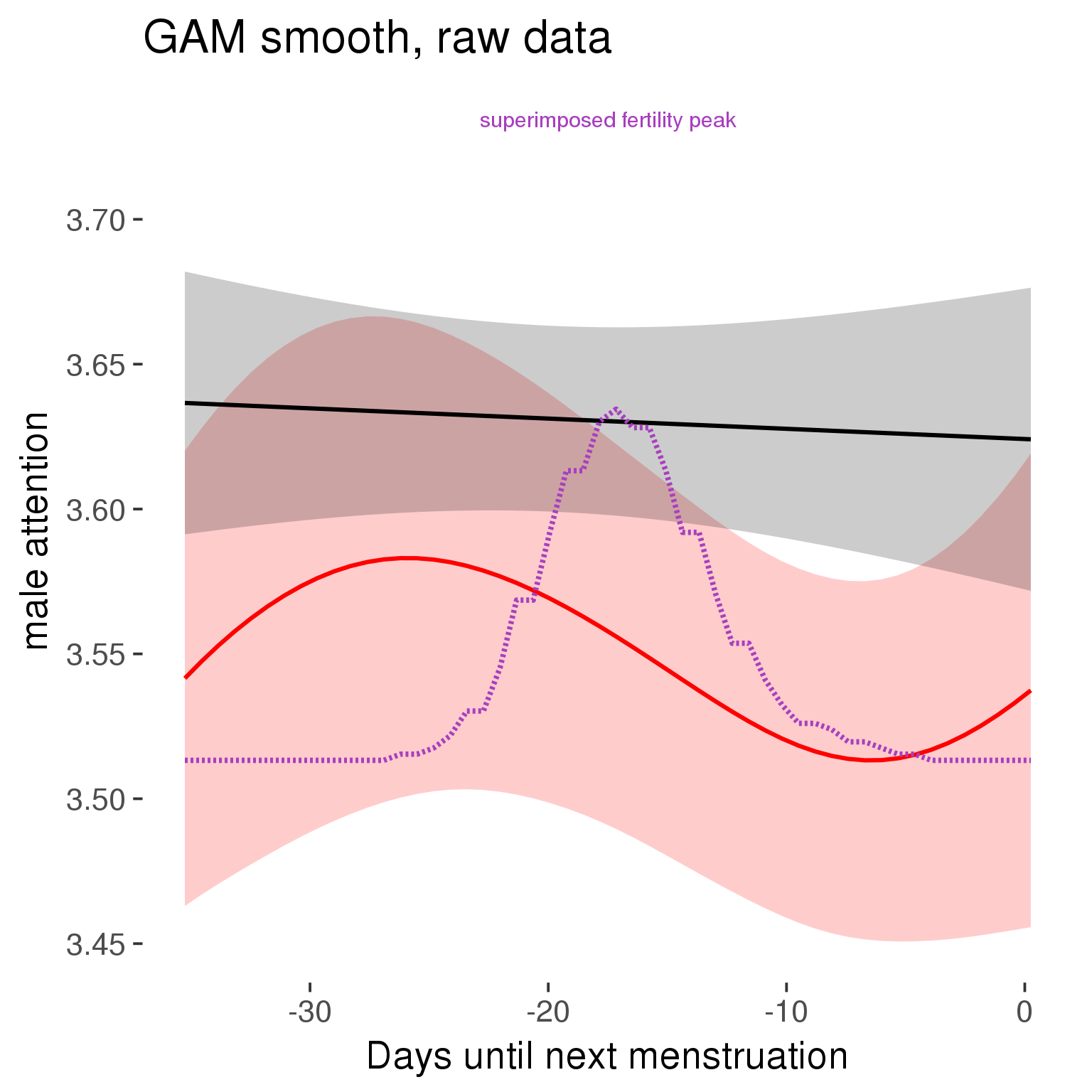
Means and standard errors over raw data
Nothing partialled out, just straight means with bootstrapped confidence intervals.
tryCatch({
trend_plot = ggplot(tmp,aes_string(x = "RCD", y = outcome, colour = "included")) +
geom_pointrange(size = 0.8, stat = 'summary', fun.data = "mean_cl_boot")
}, error = function(e){cat_message(e, "danger")})
tryCatch({
trend_data = ggplot_build(trend_plot)$data[[1]]
}, error = function(e){cat_message(e, "danger")})
trend_data$RCD = round(trend_data$x)
trend_data = left_join(trend_data, tmp %>% select(real, RCD,fertile) %>% unique(), by = "RCD")
trend_data %>%
filter(real == TRUE) %>%
mutate(superimposed = ( ( (fertile - 0.01)/0.58) * (max(y)-min(y) ) ) + min(y) ) ->
trend_data
plot3 = ggplot(trend_data) +
geom_pointrange(aes(x = x, y = y, ymin = ymin,ymax = ymax, colour = factor(group)), size = 0.8, stat = "identity", alpha = 0.6, position = position_dodge(width = .5)) +
scale_x_continuous("Days until next menstruation") +
geom_line(aes(x= x, y = superimposed), color = "#a83fbf", size = 1, linetype = 'dashed') +
annotate("text",x = mean(trend_data$x), y = max(trend_data$superimposed,na.rm=T) + 0.1, label = 'superimposed fertility peak', color = "#a83fbf") +
scale_y_continuous(outcome_label) +
ggtitle("Means with standard errors, raw data") +
scale_color_manual("Contraception status",values = c("2"="black","1"= "red"), labels = c("2"="hormonally\ncontracepting","1"="cycling"), guide = F) +
scale_fill_manual("Contraception status",values = c("2"="black","1"= "red"), labels = c("2"="hormonally\ncontracepting","1"="cycling"), guide = F)
suppressWarnings(print(plot3))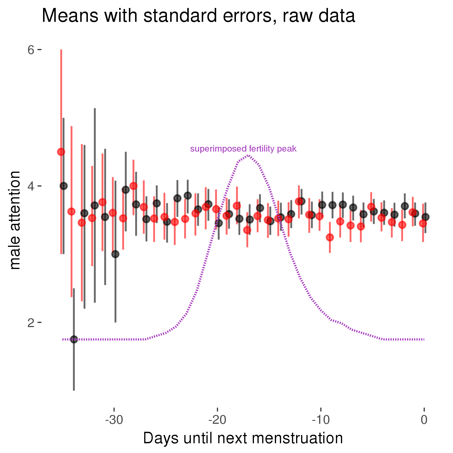
Forward-counted
model %>%
plot_curve(diary %>% filter(minimum_cycle_length_diary <= 36, minimum_cycle_length_diary > 20) %>% mutate(RCD = FCD, fertile = prc_stirn_b_forward_counted), caption_x = "Days since last menstruation")outcome = names(model@frame)[1]
outcome_label = recode(str_replace_all(str_replace_all(str_replace_all(outcome, "_", " "), " pair", "-pair"), " 1", ""),
"desirability 1" = "self-perceived desirability",
"NARQ admiration" = "narcissistic admiration",
"NARQ rivalry" = "narcissistic rivalry",
"extra-pair" = "extra-pair desire & behaviour",
"had sexual intercourse" = "sexual intercourse")
library(ggplot2)
# form a subset and run the model without the hormonal contraception and the fertility predictors
tmp = diary %>%
filter(!is.na(fertile), !is.na(included),
RCD > -1 * minimum_cycle_length_diary, RCD > -40)
new_form = update.formula(formula(model), new = . ~ . - fertile * included)
tmp$residuals = residuals(update(model, new_form, data = tmp , na.action = na.exclude))
tmp = tmp %>%
filter(!is.na(RCD), !is.na(residuals))
rcd_min = min(tmp$RCD)
tmp$real = FALSE
tmp_before = tmp
tmp_before$RCD = tmp_before$RCD + min(tmp$RCD) - 1
tmp_after = tmp
tmp_after$RCD = tmp_after$RCD - min(tmp$RCD) + 1
tmp$real = TRUE
tmp = bind_rows(tmp_before %>% filter(RCD > rcd_min - 11), tmp, tmp_after %>% filter(RCD < 11))GAM smooth on residuals
Here, we partialled out menstruation and individual random effects, then superimposed estimated probability of being in the fertile window scaled to the range of the estimated means. To address the periodicity of the cycle, we prepended and appended ten days of the timeseries to the end and the beginning of the timeseries. We then estimated the GAM and cut off the appended subsets before plotting.
tryCatch({
trend_plot = ggplot(tmp,aes(x = RCD, y = residuals, colour = included)) +
stat_smooth(geom = 'smooth',size = 0.8, fill = "#9ECAE1", method = 'gam', formula = y ~ s(x))
}, error = function(e){cat_message(e, "danger")})
tryCatch({
trend_data = ggplot_build(trend_plot)$data[[1]]
}, error = function(e){cat_message(e, "danger")})
trend_data$RCD = round(trend_data$x)
trend_data = left_join(trend_data, tmp %>% select(real, RCD,fertile) %>% unique(), by = "RCD")
trend_data %>%
filter(real == TRUE) %>%
mutate(superimposed = ( ( (fertile - 0.01)/0.58) * (max(y)-min(y) ) ) + min(y) ) ->
trend_data
ggplot(trend_data) +
geom_ribbon(aes(x = x, ymin = ymin, ymax = ymax, fill = factor(group)), alpha = 0.2) +
geom_line(aes(x = x, y = y, colour = factor(group)), size = 0.8, stat = "identity") +
scale_x_continuous(caption_x) +
geom_line(aes(x = x, y = superimposed), color = "#a83fbf", size = 1, linetype = 'dashed') +
annotate("text",x = mean(trend_data$x), y = max(trend_data$superimposed,na.rm=T) + 0.1, label = 'superimposed fertility peak', color = "#a83fbf") +
scale_y_continuous(outcome_label) +
ggtitle("GAM smooth, residuals") +
scale_color_manual("Contraception status",values = c("2"="black","1"= "red"), labels = c("2"="hormonally\ncontracepting","1"="cycling"), guide = F) +
scale_fill_manual("Contraception status",values = c("2"="black","1"= "red"), labels = c("2"="hormonally\ncontracepting","1"="cycling"), guide = F)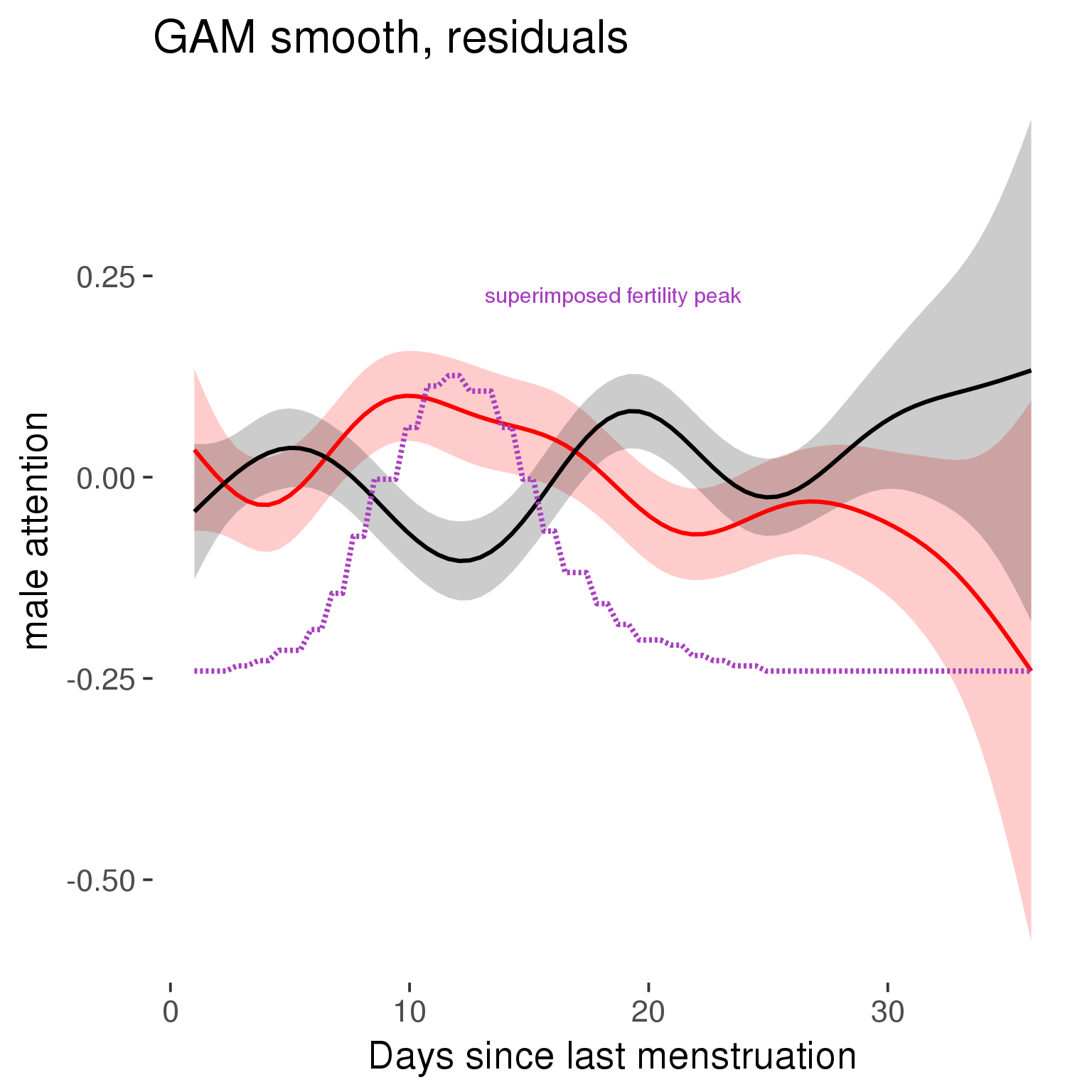
GAM smooth on raw data
As before, but without partialling anything out.
tryCatch({
trend_plot = ggplot(tmp,aes_string(x = "RCD", y = outcome, colour = "included")) +
stat_smooth(geom = 'smooth',size = 0.8, fill = "#9ECAE1", method = 'gam', formula = y ~ s(x))
}, error = function(e){cat_message(e, "danger")})
tryCatch({
trend_data = ggplot_build(trend_plot)$data[[1]]
}, error = function(e){cat_message(e, "danger")})
trend_data$RCD = round(trend_data$x)
trend_data = left_join(trend_data, tmp %>% select(real, RCD,fertile) %>% unique(), by = "RCD")
trend_data %>%
filter(real == TRUE) %>%
mutate(superimposed = ( ( (fertile - 0.01)/0.58) * (max(y)-min(y) ) ) + min(y) ) ->
trend_data
plot1b = ggplot(trend_data) +
geom_ribbon(aes(x = x, ymin = ymin, ymax = ymax, fill = factor(group)), alpha = 0.2) +
geom_line(aes(x = x, y = y, colour = factor(group)), size = 0.8, stat = "identity") +
scale_x_continuous(caption_x) +
geom_line(aes(x = x, y = superimposed), color = "#a83fbf", size = 1, linetype = 'dashed') +
annotate("text",x = mean(trend_data$x), y = max(trend_data$superimposed,na.rm=T) + 0.1, label = 'superimposed fertility peak', color = "#a83fbf") +
scale_y_continuous(outcome_label) +
ggtitle("GAM smooth, raw data") +
scale_color_manual("Contraception status",values = c("2"="black","1"= "red"), labels = c("2"="hormonally\ncontracepting","1"="cycling"), guide = F) +
scale_fill_manual("Contraception status",values = c("2"="black","1"= "red"), labels = c("2"="hormonally\ncontracepting","1"="cycling"), guide = F)
suppressWarnings(print(plot1b))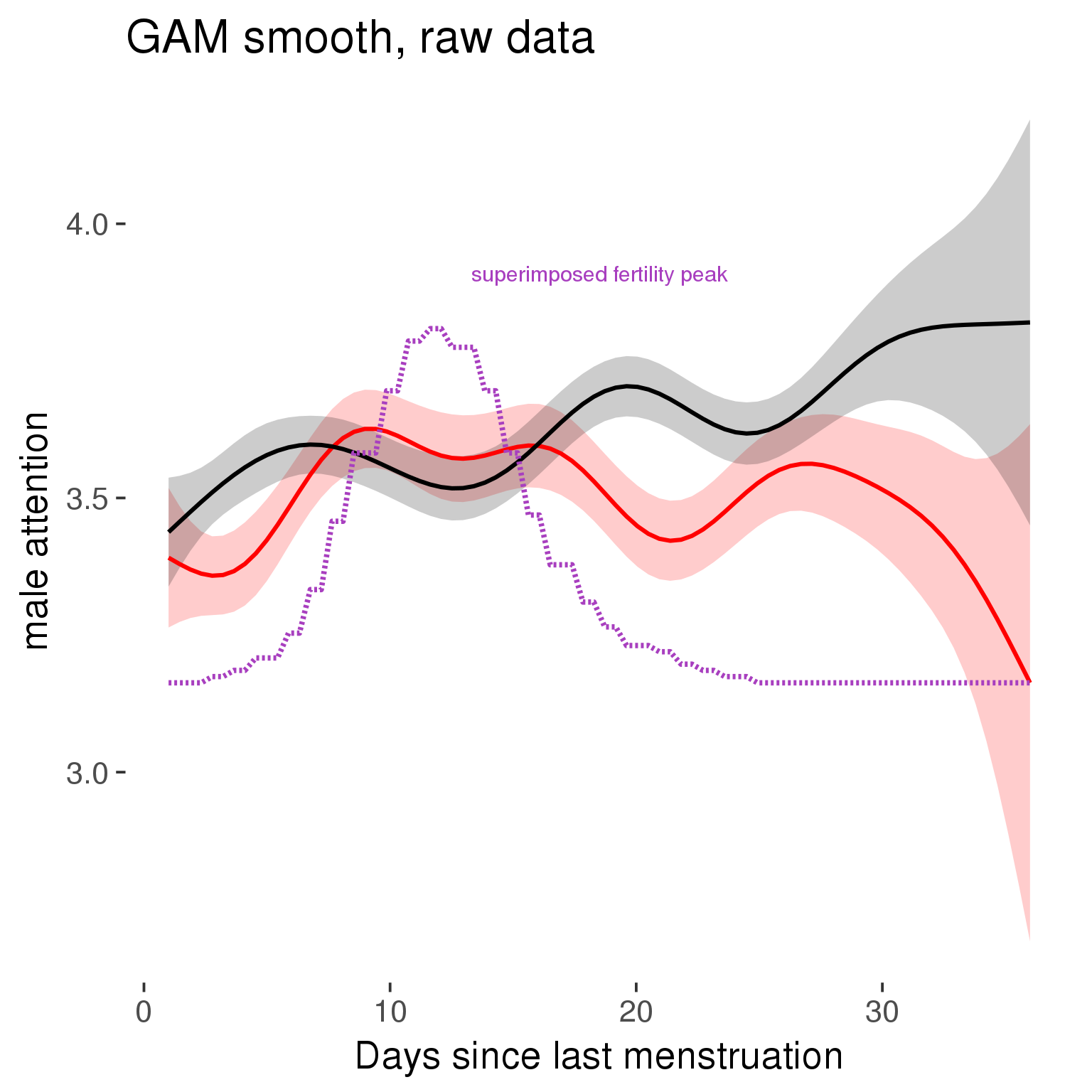
Means and standard errors over raw data
Nothing partialled out, just straight means with bootstrapped confidence intervals.
tryCatch({
trend_plot = ggplot(tmp,aes_string(x = "RCD", y = outcome, colour = "included")) +
geom_pointrange(size = 0.8, stat = 'summary', fun.data = "mean_cl_boot")
}, error = function(e){cat_message(e, "danger")})
tryCatch({
trend_data = ggplot_build(trend_plot)$data[[1]]
}, error = function(e){cat_message(e, "danger")})
trend_data$RCD = round(trend_data$x)
trend_data = left_join(trend_data, tmp %>% select(real, RCD,fertile) %>% unique(), by = "RCD")
trend_data %>%
filter(real == TRUE) %>%
mutate(superimposed = ( ( (fertile - 0.01)/0.58) * (max(y)-min(y) ) ) + min(y) ) ->
trend_data
plot3 = ggplot(trend_data) +
geom_pointrange(aes(x = x, y = y, ymin = ymin,ymax = ymax, colour = factor(group)), size = 0.8, stat = "identity", alpha = 0.6, position = position_dodge(width = .5)) +
scale_x_continuous("Days until next menstruation") +
geom_line(aes(x= x, y = superimposed), color = "#a83fbf", size = 1, linetype = 'dashed') +
annotate("text",x = mean(trend_data$x), y = max(trend_data$superimposed,na.rm=T) + 0.1, label = 'superimposed fertility peak', color = "#a83fbf") +
scale_y_continuous(outcome_label) +
ggtitle("Means with standard errors, raw data") +
scale_color_manual("Contraception status",values = c("2"="black","1"= "red"), labels = c("2"="hormonally\ncontracepting","1"="cycling"), guide = F) +
scale_fill_manual("Contraception status",values = c("2"="black","1"= "red"), labels = c("2"="hormonally\ncontracepting","1"="cycling"), guide = F)
suppressWarnings(print(plot3))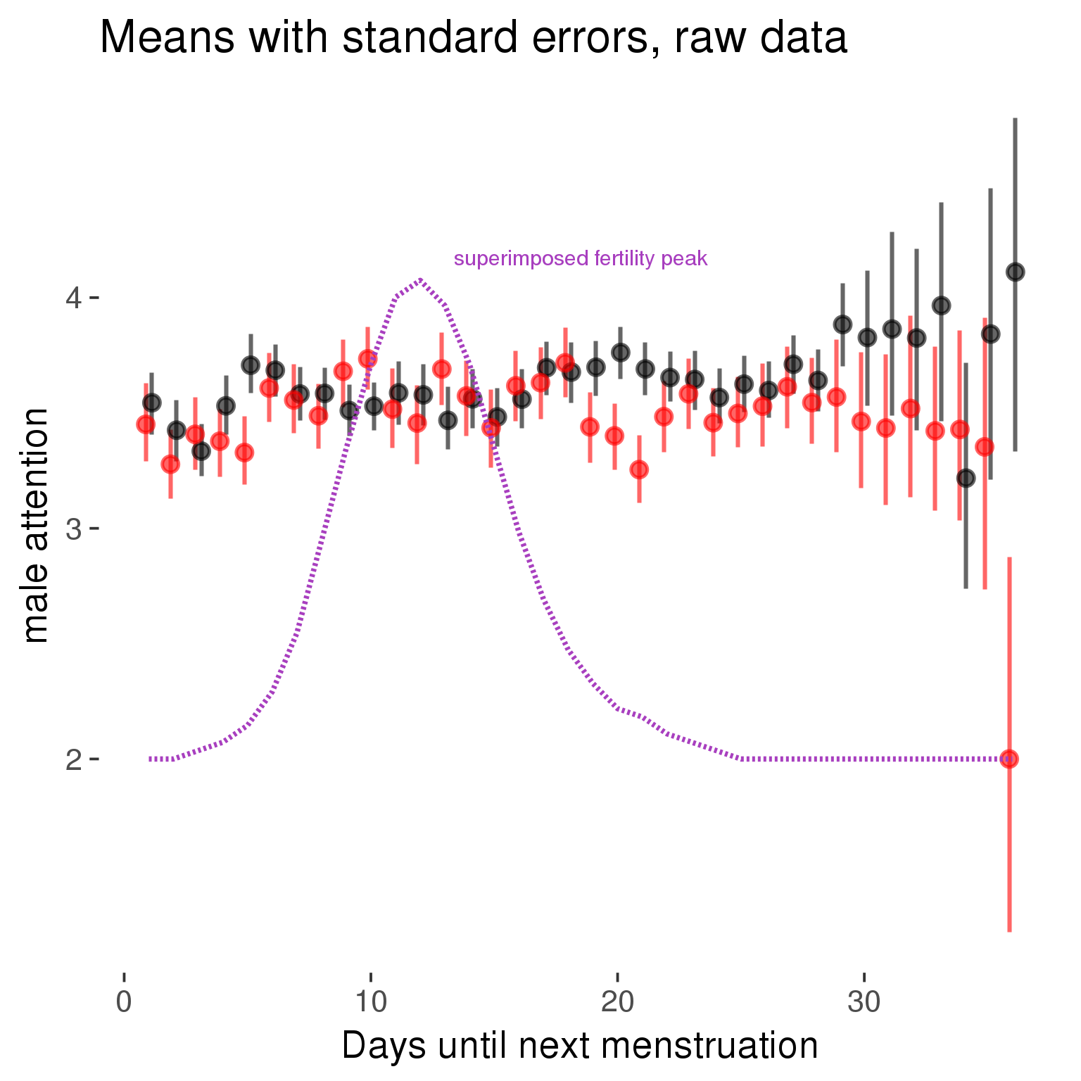
Cycle lengths from 27 to 30
Backward-counted
model %>%
plot_curve(diary %>% filter(minimum_cycle_length_diary <= 30, minimum_cycle_length_diary >= 27) %>% mutate(fertile=prc_stirn_b))outcome = names(model@frame)[1]
outcome_label = recode(str_replace_all(str_replace_all(str_replace_all(outcome, "_", " "), " pair", "-pair"), " 1", ""),
"desirability 1" = "self-perceived desirability",
"NARQ admiration" = "narcissistic admiration",
"NARQ rivalry" = "narcissistic rivalry",
"extra-pair" = "extra-pair desire & behaviour",
"had sexual intercourse" = "sexual intercourse")
library(ggplot2)
# form a subset and run the model without the hormonal contraception and the fertility predictors
tmp = diary %>%
filter(!is.na(fertile), !is.na(included),
RCD > -1 * minimum_cycle_length_diary, RCD > -40)
new_form = update.formula(formula(model), new = . ~ . - fertile * included)
tmp$residuals = residuals(update(model, new_form, data = tmp , na.action = na.exclude))
tmp = tmp %>%
filter(!is.na(RCD), !is.na(residuals))
rcd_min = min(tmp$RCD)
tmp$real = FALSE
tmp_before = tmp
tmp_before$RCD = tmp_before$RCD + min(tmp$RCD) - 1
tmp_after = tmp
tmp_after$RCD = tmp_after$RCD - min(tmp$RCD) + 1
tmp$real = TRUE
tmp = bind_rows(tmp_before %>% filter(RCD > rcd_min - 11), tmp, tmp_after %>% filter(RCD < 11))GAM smooth on residuals
Here, we partialled out menstruation and individual random effects, then superimposed estimated probability of being in the fertile window scaled to the range of the estimated means. To address the periodicity of the cycle, we prepended and appended ten days of the timeseries to the end and the beginning of the timeseries. We then estimated the GAM and cut off the appended subsets before plotting.
tryCatch({
trend_plot = ggplot(tmp,aes(x = RCD, y = residuals, colour = included)) +
stat_smooth(geom = 'smooth',size = 0.8, fill = "#9ECAE1", method = 'gam', formula = y ~ s(x))
}, error = function(e){cat_message(e, "danger")})
tryCatch({
trend_data = ggplot_build(trend_plot)$data[[1]]
}, error = function(e){cat_message(e, "danger")})
trend_data$RCD = round(trend_data$x)
trend_data = left_join(trend_data, tmp %>% select(real, RCD,fertile) %>% unique(), by = "RCD")
trend_data %>%
filter(real == TRUE) %>%
mutate(superimposed = ( ( (fertile - 0.01)/0.58) * (max(y)-min(y) ) ) + min(y) ) ->
trend_data
ggplot(trend_data) +
geom_ribbon(aes(x = x, ymin = ymin, ymax = ymax, fill = factor(group)), alpha = 0.2) +
geom_line(aes(x = x, y = y, colour = factor(group)), size = 0.8, stat = "identity") +
scale_x_continuous(caption_x) +
geom_line(aes(x = x, y = superimposed), color = "#a83fbf", size = 1, linetype = 'dashed') +
annotate("text",x = mean(trend_data$x), y = max(trend_data$superimposed,na.rm=T) + 0.1, label = 'superimposed fertility peak', color = "#a83fbf") +
scale_y_continuous(outcome_label) +
ggtitle("GAM smooth, residuals") +
scale_color_manual("Contraception status",values = c("2"="black","1"= "red"), labels = c("2"="hormonally\ncontracepting","1"="cycling"), guide = F) +
scale_fill_manual("Contraception status",values = c("2"="black","1"= "red"), labels = c("2"="hormonally\ncontracepting","1"="cycling"), guide = F)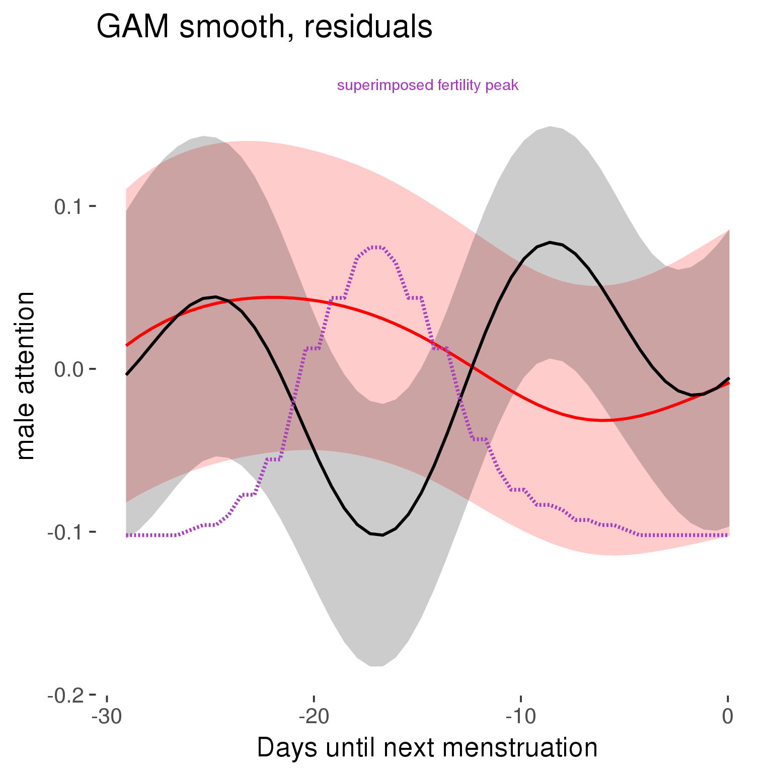
GAM smooth on raw data
As before, but without partialling anything out.
tryCatch({
trend_plot = ggplot(tmp,aes_string(x = "RCD", y = outcome, colour = "included")) +
stat_smooth(geom = 'smooth',size = 0.8, fill = "#9ECAE1", method = 'gam', formula = y ~ s(x))
}, error = function(e){cat_message(e, "danger")})
tryCatch({
trend_data = ggplot_build(trend_plot)$data[[1]]
}, error = function(e){cat_message(e, "danger")})
trend_data$RCD = round(trend_data$x)
trend_data = left_join(trend_data, tmp %>% select(real, RCD,fertile) %>% unique(), by = "RCD")
trend_data %>%
filter(real == TRUE) %>%
mutate(superimposed = ( ( (fertile - 0.01)/0.58) * (max(y)-min(y) ) ) + min(y) ) ->
trend_data
plot1b = ggplot(trend_data) +
geom_ribbon(aes(x = x, ymin = ymin, ymax = ymax, fill = factor(group)), alpha = 0.2) +
geom_line(aes(x = x, y = y, colour = factor(group)), size = 0.8, stat = "identity") +
scale_x_continuous(caption_x) +
geom_line(aes(x = x, y = superimposed), color = "#a83fbf", size = 1, linetype = 'dashed') +
annotate("text",x = mean(trend_data$x), y = max(trend_data$superimposed,na.rm=T) + 0.1, label = 'superimposed fertility peak', color = "#a83fbf") +
scale_y_continuous(outcome_label) +
ggtitle("GAM smooth, raw data") +
scale_color_manual("Contraception status",values = c("2"="black","1"= "red"), labels = c("2"="hormonally\ncontracepting","1"="cycling"), guide = F) +
scale_fill_manual("Contraception status",values = c("2"="black","1"= "red"), labels = c("2"="hormonally\ncontracepting","1"="cycling"), guide = F)
suppressWarnings(print(plot1b))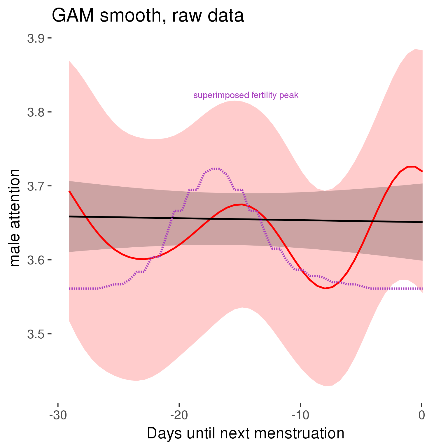
Means and standard errors over raw data
Nothing partialled out, just straight means with bootstrapped confidence intervals.
tryCatch({
trend_plot = ggplot(tmp,aes_string(x = "RCD", y = outcome, colour = "included")) +
geom_pointrange(size = 0.8, stat = 'summary', fun.data = "mean_cl_boot")
}, error = function(e){cat_message(e, "danger")})
tryCatch({
trend_data = ggplot_build(trend_plot)$data[[1]]
}, error = function(e){cat_message(e, "danger")})
trend_data$RCD = round(trend_data$x)
trend_data = left_join(trend_data, tmp %>% select(real, RCD,fertile) %>% unique(), by = "RCD")
trend_data %>%
filter(real == TRUE) %>%
mutate(superimposed = ( ( (fertile - 0.01)/0.58) * (max(y)-min(y) ) ) + min(y) ) ->
trend_data
plot3 = ggplot(trend_data) +
geom_pointrange(aes(x = x, y = y, ymin = ymin,ymax = ymax, colour = factor(group)), size = 0.8, stat = "identity", alpha = 0.6, position = position_dodge(width = .5)) +
scale_x_continuous("Days until next menstruation") +
geom_line(aes(x= x, y = superimposed), color = "#a83fbf", size = 1, linetype = 'dashed') +
annotate("text",x = mean(trend_data$x), y = max(trend_data$superimposed,na.rm=T) + 0.1, label = 'superimposed fertility peak', color = "#a83fbf") +
scale_y_continuous(outcome_label) +
ggtitle("Means with standard errors, raw data") +
scale_color_manual("Contraception status",values = c("2"="black","1"= "red"), labels = c("2"="hormonally\ncontracepting","1"="cycling"), guide = F) +
scale_fill_manual("Contraception status",values = c("2"="black","1"= "red"), labels = c("2"="hormonally\ncontracepting","1"="cycling"), guide = F)
suppressWarnings(print(plot3))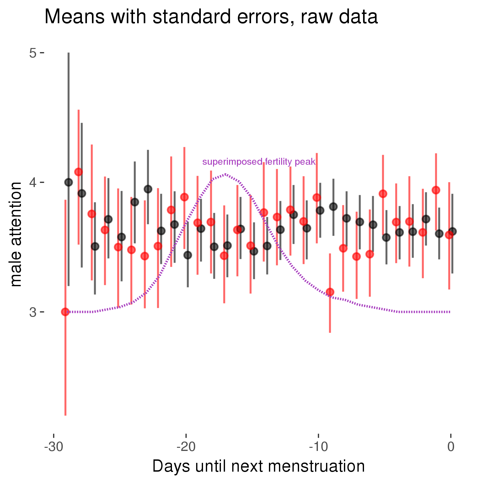
Forward-counted
model %>%
plot_curve(diary %>% filter(minimum_cycle_length_diary <= 30, minimum_cycle_length_diary >= 27) %>% mutate(RCD = FCD, fertile = prc_stirn_b_forward_counted), caption_x = "Days since last menstruation")outcome = names(model@frame)[1]
outcome_label = recode(str_replace_all(str_replace_all(str_replace_all(outcome, "_", " "), " pair", "-pair"), " 1", ""),
"desirability 1" = "self-perceived desirability",
"NARQ admiration" = "narcissistic admiration",
"NARQ rivalry" = "narcissistic rivalry",
"extra-pair" = "extra-pair desire & behaviour",
"had sexual intercourse" = "sexual intercourse")
library(ggplot2)
# form a subset and run the model without the hormonal contraception and the fertility predictors
tmp = diary %>%
filter(!is.na(fertile), !is.na(included),
RCD > -1 * minimum_cycle_length_diary, RCD > -40)
new_form = update.formula(formula(model), new = . ~ . - fertile * included)
tmp$residuals = residuals(update(model, new_form, data = tmp , na.action = na.exclude))
tmp = tmp %>%
filter(!is.na(RCD), !is.na(residuals))
rcd_min = min(tmp$RCD)
tmp$real = FALSE
tmp_before = tmp
tmp_before$RCD = tmp_before$RCD + min(tmp$RCD) - 1
tmp_after = tmp
tmp_after$RCD = tmp_after$RCD - min(tmp$RCD) + 1
tmp$real = TRUE
tmp = bind_rows(tmp_before %>% filter(RCD > rcd_min - 11), tmp, tmp_after %>% filter(RCD < 11))GAM smooth on residuals
Here, we partialled out menstruation and individual random effects, then superimposed estimated probability of being in the fertile window scaled to the range of the estimated means. To address the periodicity of the cycle, we prepended and appended ten days of the timeseries to the end and the beginning of the timeseries. We then estimated the GAM and cut off the appended subsets before plotting.
tryCatch({
trend_plot = ggplot(tmp,aes(x = RCD, y = residuals, colour = included)) +
stat_smooth(geom = 'smooth',size = 0.8, fill = "#9ECAE1", method = 'gam', formula = y ~ s(x))
}, error = function(e){cat_message(e, "danger")})
tryCatch({
trend_data = ggplot_build(trend_plot)$data[[1]]
}, error = function(e){cat_message(e, "danger")})
trend_data$RCD = round(trend_data$x)
trend_data = left_join(trend_data, tmp %>% select(real, RCD,fertile) %>% unique(), by = "RCD")
trend_data %>%
filter(real == TRUE) %>%
mutate(superimposed = ( ( (fertile - 0.01)/0.58) * (max(y)-min(y) ) ) + min(y) ) ->
trend_data
ggplot(trend_data) +
geom_ribbon(aes(x = x, ymin = ymin, ymax = ymax, fill = factor(group)), alpha = 0.2) +
geom_line(aes(x = x, y = y, colour = factor(group)), size = 0.8, stat = "identity") +
scale_x_continuous(caption_x) +
geom_line(aes(x = x, y = superimposed), color = "#a83fbf", size = 1, linetype = 'dashed') +
annotate("text",x = mean(trend_data$x), y = max(trend_data$superimposed,na.rm=T) + 0.1, label = 'superimposed fertility peak', color = "#a83fbf") +
scale_y_continuous(outcome_label) +
ggtitle("GAM smooth, residuals") +
scale_color_manual("Contraception status",values = c("2"="black","1"= "red"), labels = c("2"="hormonally\ncontracepting","1"="cycling"), guide = F) +
scale_fill_manual("Contraception status",values = c("2"="black","1"= "red"), labels = c("2"="hormonally\ncontracepting","1"="cycling"), guide = F)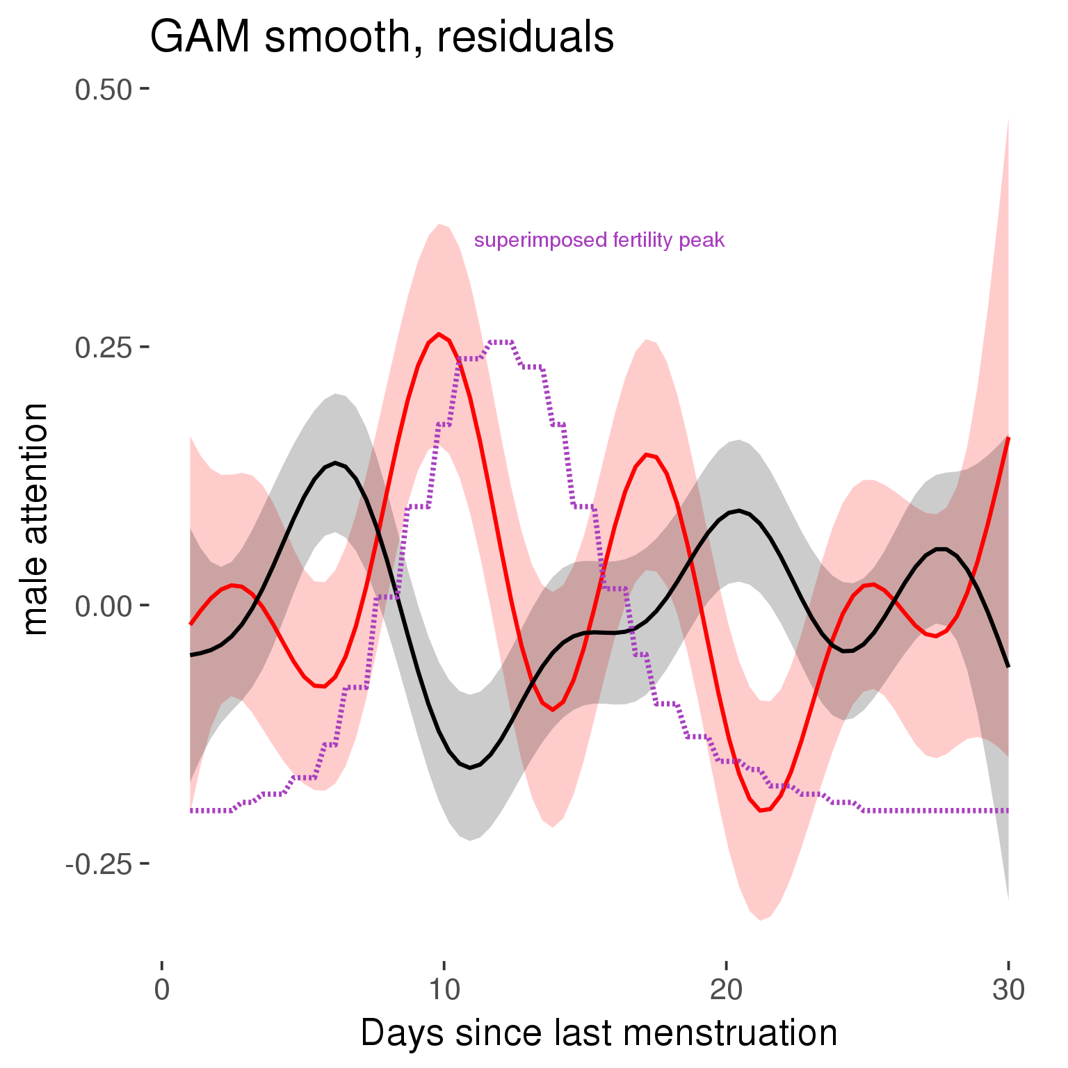
GAM smooth on raw data
As before, but without partialling anything out.
tryCatch({
trend_plot = ggplot(tmp,aes_string(x = "RCD", y = outcome, colour = "included")) +
stat_smooth(geom = 'smooth',size = 0.8, fill = "#9ECAE1", method = 'gam', formula = y ~ s(x))
}, error = function(e){cat_message(e, "danger")})
tryCatch({
trend_data = ggplot_build(trend_plot)$data[[1]]
}, error = function(e){cat_message(e, "danger")})
trend_data$RCD = round(trend_data$x)
trend_data = left_join(trend_data, tmp %>% select(real, RCD,fertile) %>% unique(), by = "RCD")
trend_data %>%
filter(real == TRUE) %>%
mutate(superimposed = ( ( (fertile - 0.01)/0.58) * (max(y)-min(y) ) ) + min(y) ) ->
trend_data
plot1b = ggplot(trend_data) +
geom_ribbon(aes(x = x, ymin = ymin, ymax = ymax, fill = factor(group)), alpha = 0.2) +
geom_line(aes(x = x, y = y, colour = factor(group)), size = 0.8, stat = "identity") +
scale_x_continuous(caption_x) +
geom_line(aes(x = x, y = superimposed), color = "#a83fbf", size = 1, linetype = 'dashed') +
annotate("text",x = mean(trend_data$x), y = max(trend_data$superimposed,na.rm=T) + 0.1, label = 'superimposed fertility peak', color = "#a83fbf") +
scale_y_continuous(outcome_label) +
ggtitle("GAM smooth, raw data") +
scale_color_manual("Contraception status",values = c("2"="black","1"= "red"), labels = c("2"="hormonally\ncontracepting","1"="cycling"), guide = F) +
scale_fill_manual("Contraception status",values = c("2"="black","1"= "red"), labels = c("2"="hormonally\ncontracepting","1"="cycling"), guide = F)
suppressWarnings(print(plot1b))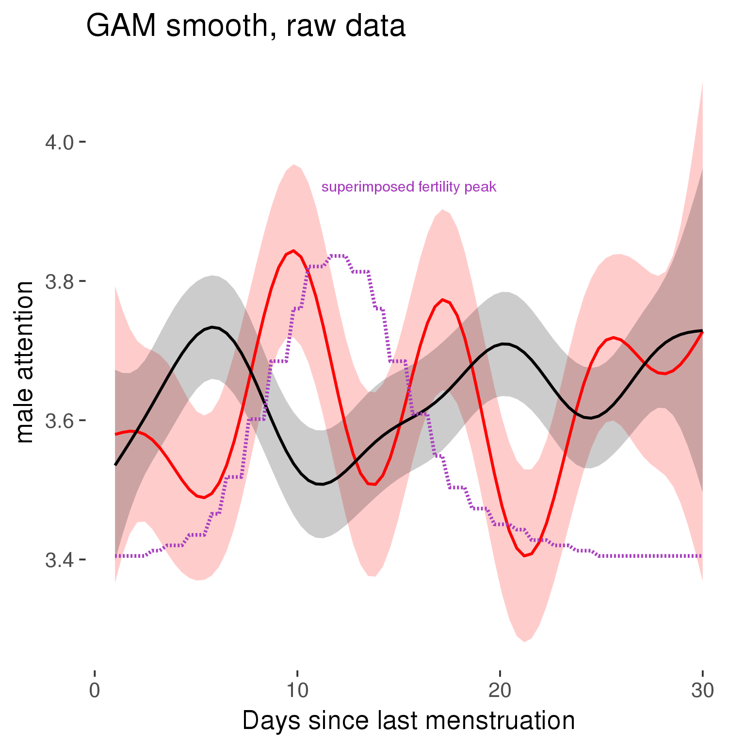
Means and standard errors over raw data
Nothing partialled out, just straight means with bootstrapped confidence intervals.
tryCatch({
trend_plot = ggplot(tmp,aes_string(x = "RCD", y = outcome, colour = "included")) +
geom_pointrange(size = 0.8, stat = 'summary', fun.data = "mean_cl_boot")
}, error = function(e){cat_message(e, "danger")})
tryCatch({
trend_data = ggplot_build(trend_plot)$data[[1]]
}, error = function(e){cat_message(e, "danger")})
trend_data$RCD = round(trend_data$x)
trend_data = left_join(trend_data, tmp %>% select(real, RCD,fertile) %>% unique(), by = "RCD")
trend_data %>%
filter(real == TRUE) %>%
mutate(superimposed = ( ( (fertile - 0.01)/0.58) * (max(y)-min(y) ) ) + min(y) ) ->
trend_data
plot3 = ggplot(trend_data) +
geom_pointrange(aes(x = x, y = y, ymin = ymin,ymax = ymax, colour = factor(group)), size = 0.8, stat = "identity", alpha = 0.6, position = position_dodge(width = .5)) +
scale_x_continuous("Days until next menstruation") +
geom_line(aes(x= x, y = superimposed), color = "#a83fbf", size = 1, linetype = 'dashed') +
annotate("text",x = mean(trend_data$x), y = max(trend_data$superimposed,na.rm=T) + 0.1, label = 'superimposed fertility peak', color = "#a83fbf") +
scale_y_continuous(outcome_label) +
ggtitle("Means with standard errors, raw data") +
scale_color_manual("Contraception status",values = c("2"="black","1"= "red"), labels = c("2"="hormonally\ncontracepting","1"="cycling"), guide = F) +
scale_fill_manual("Contraception status",values = c("2"="black","1"= "red"), labels = c("2"="hormonally\ncontracepting","1"="cycling"), guide = F)
suppressWarnings(print(plot3))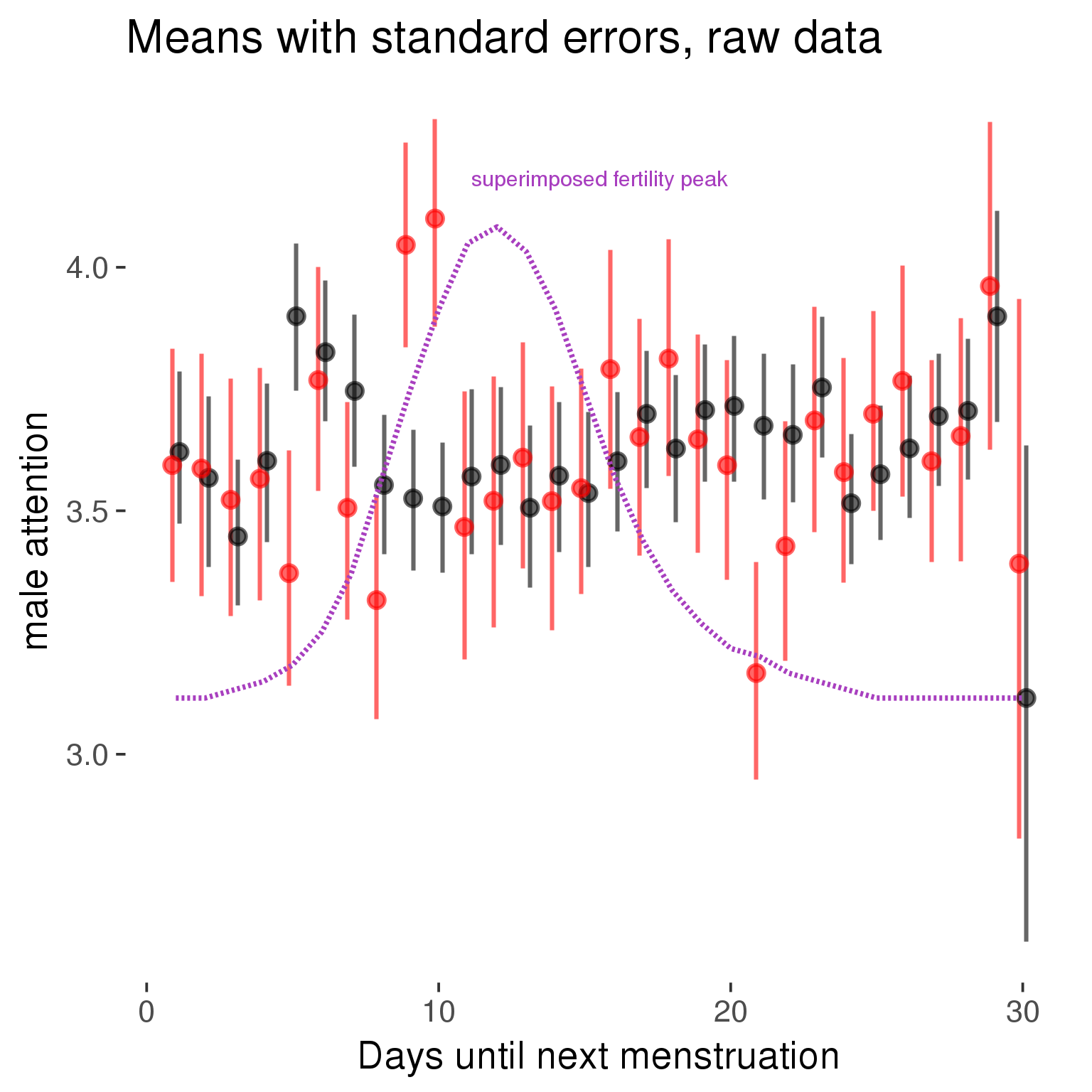
Robustness checks
M_r1: Random slopes for conception risk and menstruation
tryCatch({
# refit model with random effects for fertile and menstruation dummies
with_ind_diff = update(model, formula = . ~ . - (1| person) + (1 + fertile + menstruation | person))
# pull the random effects, format as tibble
rand = coef(with_ind_diff)$person %>%
tibble::rownames_to_column("person") %>%
mutate(person = as.numeric(person))
# pull the fixed effects
fixd = data.frame(fixef(with_ind_diff)) %>%
tibble::rownames_to_column("effect")
names(fixd) = c("effect", "pop_effect_size")
# pull apart the coefficients so that we can account for the fact that the random effect variation implicitly includes HC explaining the mean population-level effect of fertile/menstruation dummies among HC users
fixd = fixd %>%
separate(effect, c("included", "effect"), sep = ":", fill = "left") %>%
mutate(included = if_else(is.na(included), "cycling", str_replace(included, "included", "")))
fixd[2,c("included", "effect")] = c("horm_contra", "(Intercept)")
rand = rand %>%
# merge diary data on the random effects, so that we know who is a HC users and who isn't
inner_join(diary %>% select(person, included) %>% unique(), by = 'person') %>%
# gather into long format, to have the dataset by predictor
gather(effect, value, -person, -included) %>%
inner_join(fixd, by = c('effect', 'included')) %>%
# pull the fixed effects
mutate(
# only for those who are HC users, add the moderated population effect size for this effect (the random effects have the reference category mean)
value = if_else(included == "horm_contra", value + pop_effect_size, value),
effect = recode(effect, "includedhorm_contra" = "HC user",
"includedhorm_contra:fertile" = "HC user x fertile",
"includedhorm_contra:menstruationpre" = "HC user x premens.",
"includedhorm_contra:menstruationyes" = "HC user x mens.",
"menstruationyes" = "mens.",
"menstruationpre" = "premens.")) %>%
group_by(included, effect) %>%
# filter out predictors that aren't modelled as varying/random
filter(sd(value) > 0)
# plot dot plot of random effects
print(
ggplot(rand, aes(x = included, y = value, color = included, fill = included)) +
facet_wrap( ~ effect, scales = "free") +
# geom_violin(alpha = 0.4, size = 0) +
geom_dotplot(binaxis='y', dotsize = 0.1, method = "histodot") +
# geom_jitter(alpha = 0.05) +
coord_flip() +
geom_pointrange(stat = 'summary', fun.data = 'mean_sdl', color = 'darkred', size = 1.2) +
scale_color_manual("Contraception status", values = c("horm_contra"="black","cycling"= "red"), labels = c("horm_contra"="hormonally\ncontracepting","cycling"="cycling"), guide = F) +
scale_fill_manual("Contraception status", values = c("horm_contra"="black","cycling"= "red"), labels = c("horm_contra"="hormonally\ncontracepting","1"="cycling"), guide = F) +
ggtitle("M_r1: allowing participant-varying slopes", subtitle = "for the conception risk measure and the menstruation dummies") +
scale_x_discrete("Hormonal contraception", breaks = c("horm_contra", "cycling"), labels = c("yes", "no")) +
scale_y_continuous("Random effect size distribution"))
print_summary(with_ind_diff)
cat(pander(anova(model, with_ind_diff)))
}, error = function(e){
with_ind_diff = model
cat_message(e, "danger")
})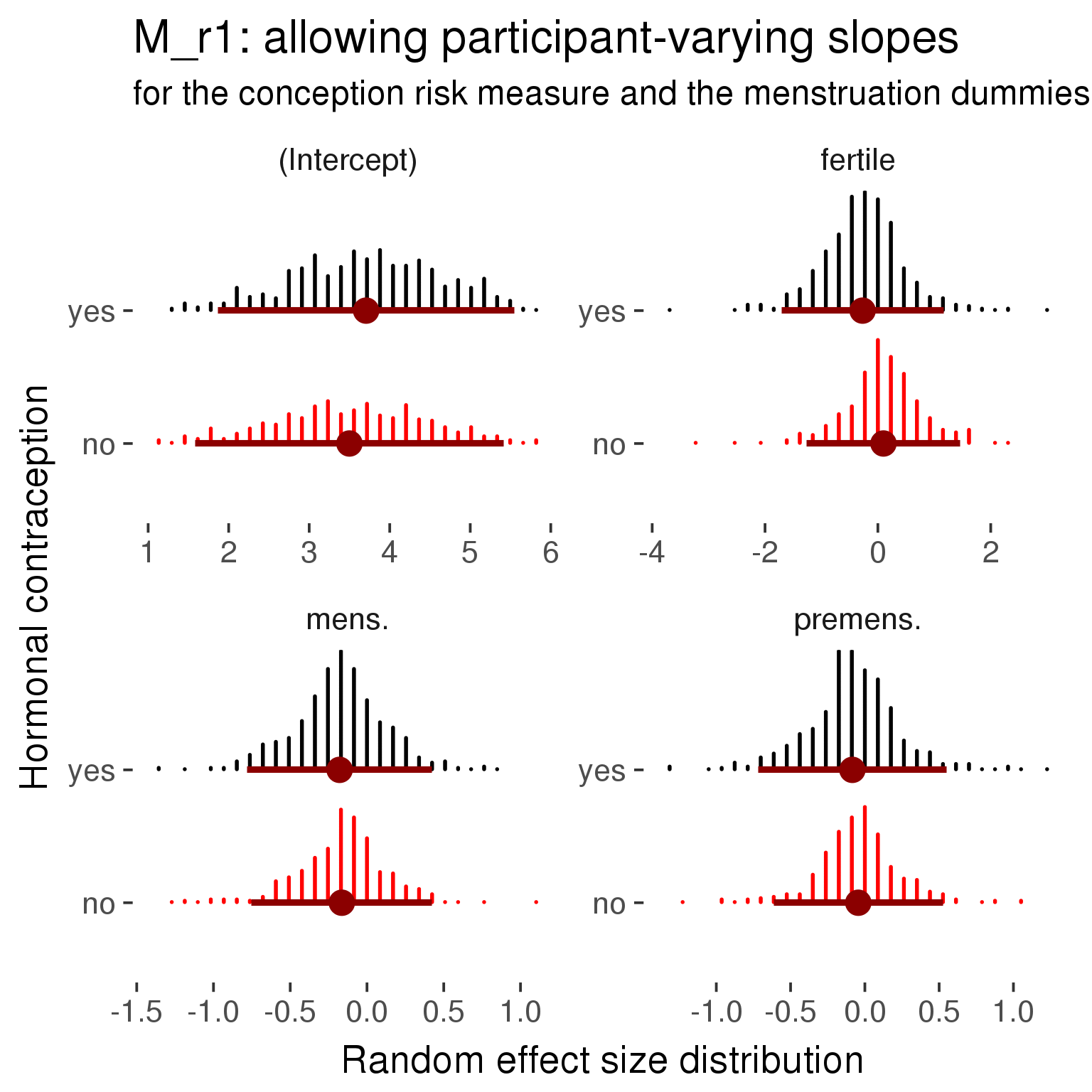
Linear mixed model fit by REML ['lmerMod']
Formula: male_attention_1 ~ included + menstruation + fertile + fertile_mean +
(1 + fertile + menstruation | person) + included:menstruation + included:fertile
Data: diary
REML criterion at convergence: 101715
Scaled residuals:
Min 1Q Median 3Q Max
-2.9238 -0.7176 -0.0078 0.7008 2.8126
Random effects:
Groups Name Variance Std.Dev. Corr
person (Intercept) 1.117 1.057
fertile 1.690 1.300 -0.27
menstruationpre 0.355 0.596 -0.30 0.51
menstruationyes 0.341 0.584 -0.26 0.37 0.46
Residual 2.330 1.526
Number of obs: 26680, groups: person, 1054
Fixed effects:
Estimate Std. Error t value
(Intercept) 3.4995 0.0951 36.8
includedhorm_contra 0.2074 0.0796 2.6
menstruationpre -0.0442 0.0580 -0.8
menstruationyes -0.1639 0.0553 -3.0
fertile 0.0991 0.1200 0.8
fertile_mean 0.0259 0.4354 0.1
includedhorm_contra:menstruationpre -0.0398 0.0744 -0.5
includedhorm_contra:menstruationyes -0.0144 0.0720 -0.2
includedhorm_contra:fertile -0.3700 0.1523 -2.4
Correlation of Fixed Effects:
(Intr) incld_ mnstrtnp mnstrtny fertil frtl_m inclddhrm_cntr:mnstrtnp
inclddhrm_c -0.485
menstrutnpr -0.256 0.312
menstrutnys -0.242 0.291 0.410
fertile -0.229 0.352 0.473 0.375
fertile_men -0.759 -0.028 -0.006 -0.002 -0.084
inclddhrm_cntr:mnstrtnp 0.210 -0.394 -0.779 -0.319 -0.367 -0.008
inclddhrm_cntr:mnstrtny 0.192 -0.362 -0.315 -0.768 -0.287 -0.007 0.400
inclddhrm_cntr:f 0.222 -0.447 -0.372 -0.296 -0.783 0.012 0.473
inclddhrm_cntr:mnstrtny
inclddhrm_c
menstrutnpr
menstrutnys
fertile
fertile_men
inclddhrm_cntr:mnstrtnp
inclddhrm_cntr:mnstrtny
inclddhrm_cntr:f 0.371
refitting model(s) with ML (instead of REML)
| Df | AIC | BIC | logLik | deviance | Chisq | Chi Df | Pr(>Chisq) | |
|---|---|---|---|---|---|---|---|---|
| object | 11 | 101947 | 102037 | -50963 | 101925 | NA | NA | NA |
| ..1 | 20 | 101724 | 101888 | -50842 | 101684 | 241.2 | 9 | 7.118e-47 |
robustness_check_ovu_shift(model, diary)M_e: Exclusion criteria
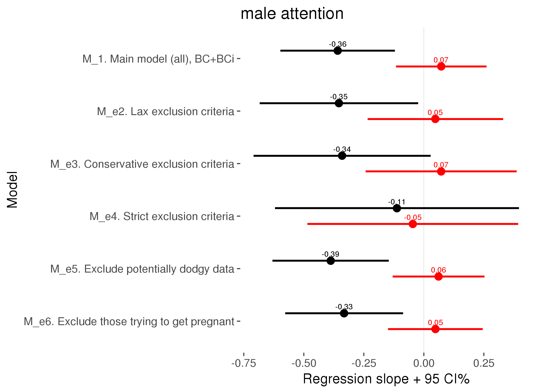
M_p: Predictors
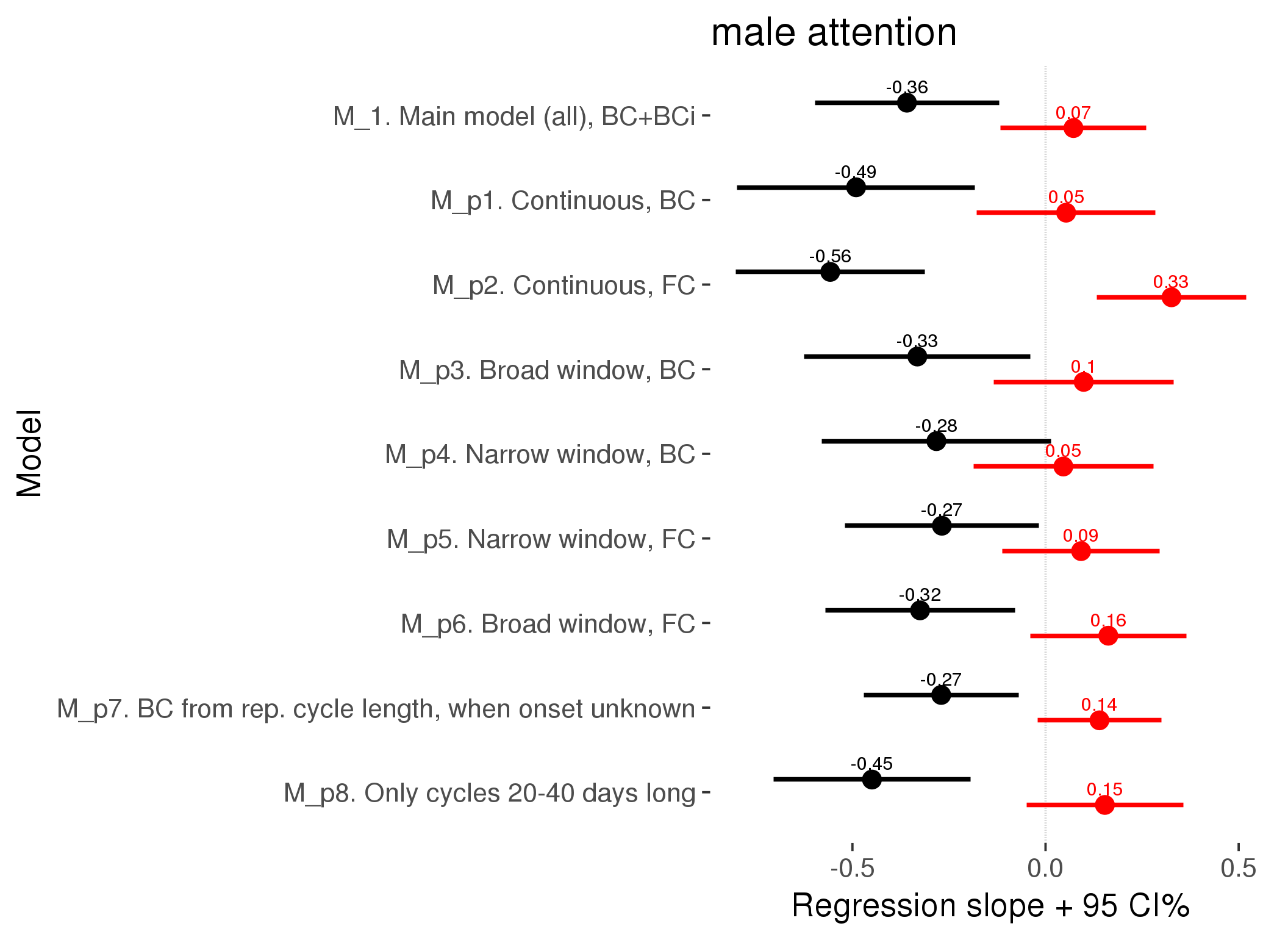
M_c: Covariates, controls, autocorrelation
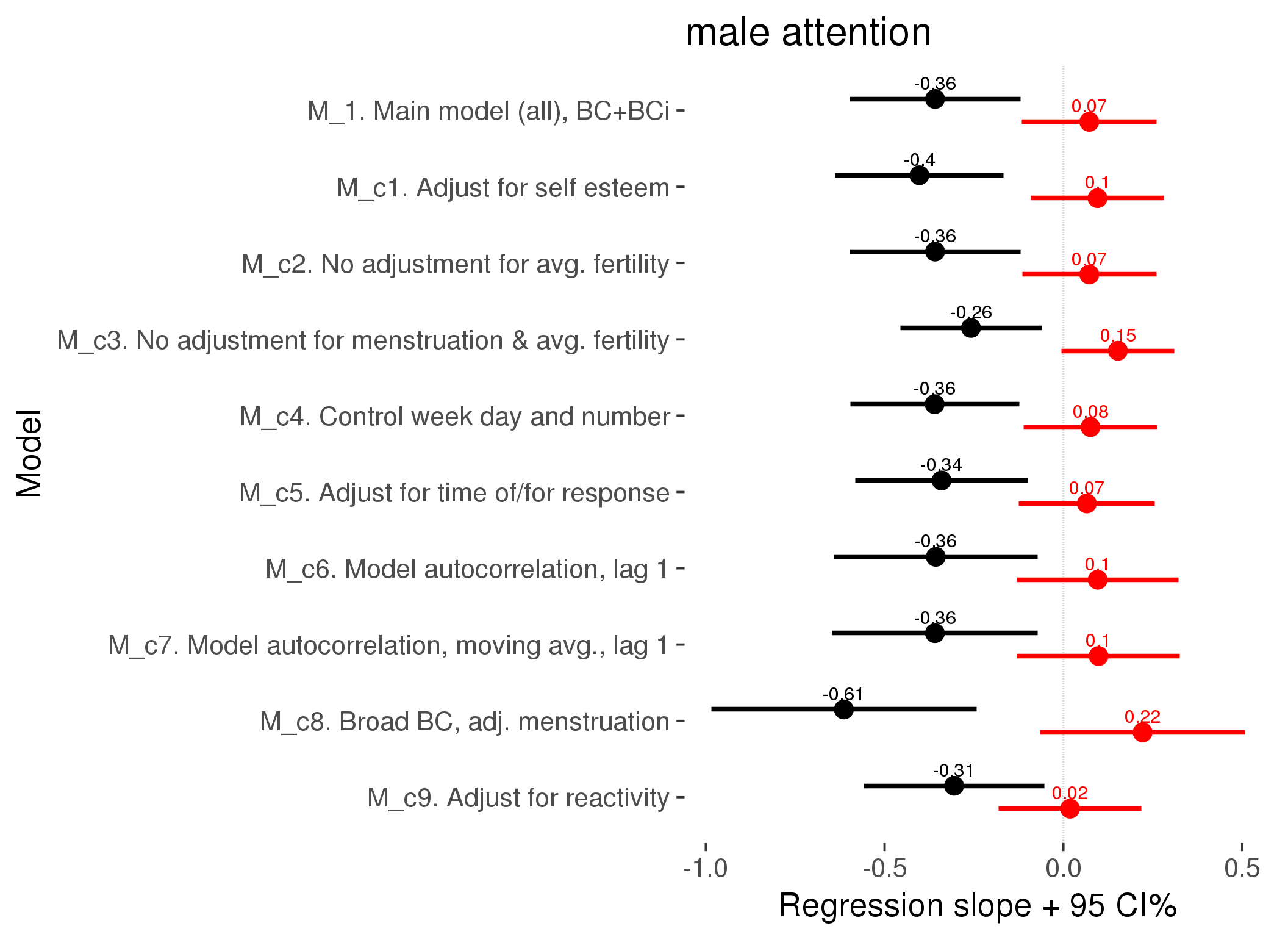
Linear mixed model fit by REML ['lmerMod']
REML criterion at convergence: 93016
Scaled residuals:
Min 1Q Median 3Q Max
-2.8619 -0.7329 -0.0018 0.7124 2.9746
Random effects:
Groups Name Variance Std.Dev.
person (Intercept) 1.008 1.004
Xr.2 s(days_filled_out):includedhorm_contra 0.223 0.473
Xr.1 s(days_filled_out):includedcycling 0.109 0.330
Xr.0 s(day_number):includedhorm_contra 0.267 0.517
Xr s(day_number):includedcycling 0.231 0.481
Residual 2.415 1.554
Number of obs: 24377, groups: person, 1054; Xr.2, 8; Xr.1, 8; Xr.0, 8; Xr, 8
Fixed effects:
Estimate Std. Error t value
X(Intercept) 3.47870 0.09419 36.9
Xincludedhorm_contra 0.18312 0.07792 2.4
Xmenstruationpre -0.05043 0.04949 -1.0
Xmenstruationyes -0.18751 0.04749 -3.9
Xfertile 0.01866 0.10191 0.2
Xfertile_mean 0.08267 0.43171 0.2
Xincludedhorm_contra:menstruationpre -0.03129 0.06349 -0.5
Xincludedhorm_contra:menstruationyes 0.00835 0.06218 0.1
Xincludedhorm_contra:fertile -0.30568 0.12892 -2.4
Xs(day_number):includedcyclingFx1 0.26465 0.16567 1.6
Xs(day_number):includedhorm_contraFx1 0.62711 0.17217 3.6
Xs(days_filled_out):includedcyclingFx1 -0.12873 0.14676 -0.9
Xs(days_filled_out):includedhorm_contraFx1 -0.54021 0.16757 -3.2
Family: gaussian
Link function: identity
Formula:
male_attention_1 ~ included + menstruation + fertile + fertile_mean +
s(day_number, by = included) + s(days_filled_out, by = included) +
included:menstruation + included:fertile
Parametric coefficients:
Estimate Std. Error t value Pr(>|t|)
(Intercept) 3.47870 0.09419 36.93 < 2e-16 ***
includedhorm_contra 0.18312 0.07792 2.35 0.019 *
menstruationpre -0.05043 0.04949 -1.02 0.308
menstruationyes -0.18751 0.04749 -3.95 0.000079 ***
fertile 0.01866 0.10191 0.18 0.855
fertile_mean 0.08267 0.43171 0.19 0.848
includedhorm_contra:menstruationpre -0.03129 0.06349 -0.49 0.622
includedhorm_contra:menstruationyes 0.00835 0.06218 0.13 0.893
includedhorm_contra:fertile -0.30568 0.12892 -2.37 0.018 *
---
Signif. codes: 0 '***' 0.001 '**' 0.01 '*' 0.05 '.' 0.1 ' ' 1
Approximate significance of smooth terms:
edf Ref.df F p-value
s(day_number):includedcycling 3.72 3.72 1.76 0.15
s(day_number):includedhorm_contra 4.13 4.13 6.97 0.0000111 ***
s(days_filled_out):includedcycling 2.78 2.78 1.86 0.12
s(days_filled_out):includedhorm_contra 3.88 3.88 7.68 0.0000056 ***
---
Signif. codes: 0 '***' 0.001 '**' 0.01 '*' 0.05 '.' 0.1 ' ' 1
R-sq.(adj) = 0.00258
lmer.REML = 93016 Scale est. = 2.4149 n = 24377
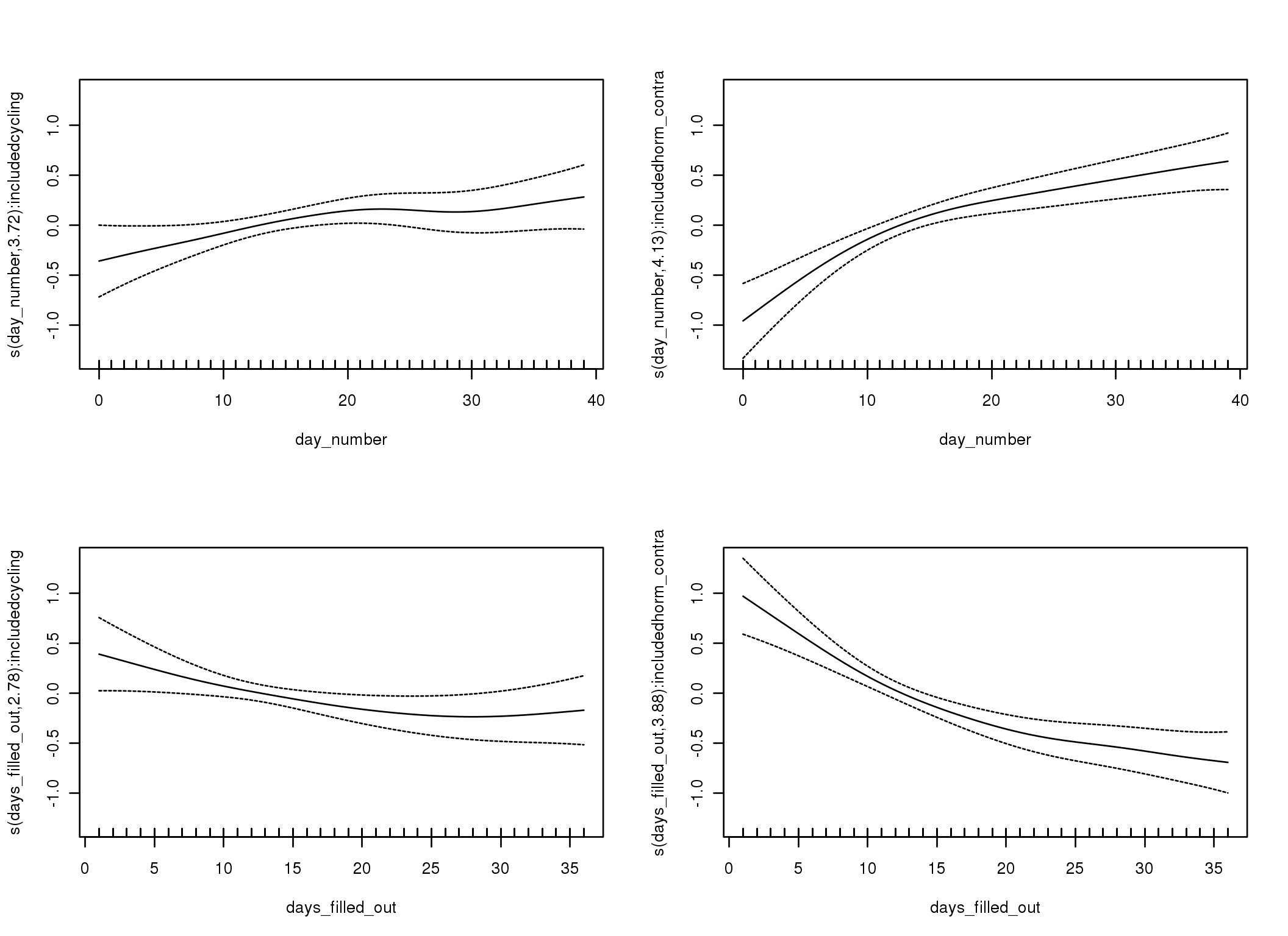
Linear mixed-effects model fit by REML
Data: diary
AIC BIC logLik
100560 100658 -50268
Random effects:
Formula: ~1 | person
(Intercept) Residual
StdDev: 0.9625 1.582
Correlation Structure: ARMA(1,0)
Formula: ~day_number | person
Parameter estimate(s):
Phi1
0.2699
Fixed effects: male_attention_1 ~ included * (menstruation + fertile) + fertile_mean
Value Std.Error DF t-value p-value
(Intercept) 3.503 0.0947 25620 37.00 0.0000
includedhorm_contra 0.202 0.0781 1051 2.59 0.0098
menstruationpre -0.050 0.0546 25620 -0.92 0.3567
menstruationyes -0.162 0.0509 25620 -3.18 0.0015
fertile 0.096 0.1152 25620 0.83 0.4052
fertile_mean 0.073 0.4376 1051 0.17 0.8679
includedhorm_contra:menstruationpre -0.035 0.0701 25620 -0.50 0.6172
includedhorm_contra:menstruationyes 0.018 0.0665 25620 0.26 0.7913
includedhorm_contra:fertile -0.357 0.1456 25620 -2.45 0.0143
Correlation:
(Intr) incld_ mnstrtnp mnstrtny fertil frtl_m inclddhrm_cntr:mnstrtnp
includedhorm_contra -0.478
menstruationpre -0.223 0.277
menstruationyes -0.217 0.268 0.399
fertile -0.213 0.348 0.431 0.363
fertile_mean -0.766 -0.030 -0.007 -0.005 -0.094
includedhorm_contra:menstruationpre 0.182 -0.346 -0.778 -0.311 -0.335 -0.006
includedhorm_contra:menstruationyes 0.173 -0.327 -0.306 -0.766 -0.277 -0.005 0.385
includedhorm_contra:fertile 0.214 -0.440 -0.341 -0.287 -0.786 0.014 0.431
inclddhrm_cntr:mnstrtny
includedhorm_contra
menstruationpre
menstruationyes
fertile
fertile_mean
includedhorm_contra:menstruationpre
includedhorm_contra:menstruationyes
includedhorm_contra:fertile 0.357
Standardized Within-Group Residuals:
Min Q1 Med Q3 Max
-2.77118 -0.74579 -0.00276 0.71800 2.80207
Number of Observations: 26680
Number of Groups: 1054
Linear mixed-effects model fit by REML
Data: diary
AIC BIC logLik
100555 100661 -50264
Random effects:
Formula: ~1 | person
(Intercept) Residual
StdDev: 0.9598 1.583
Correlation Structure: ARMA(1,1)
Formula: ~day_number | person
Parameter estimate(s):
Phi1 Theta1
0.33213 -0.06688
Fixed effects: male_attention_1 ~ included * (menstruation + fertile) + fertile_mean
Value Std.Error DF t-value p-value
(Intercept) 3.501 0.0947 25620 36.95 0.0000
includedhorm_contra 0.203 0.0782 1051 2.60 0.0095
menstruationpre -0.049 0.0548 25620 -0.89 0.3736
menstruationyes -0.161 0.0512 25620 -3.15 0.0016
fertile 0.098 0.1162 25620 0.85 0.3976
fertile_mean 0.077 0.4380 1051 0.18 0.8610
includedhorm_contra:menstruationpre -0.036 0.0704 25620 -0.52 0.6063
includedhorm_contra:menstruationyes 0.017 0.0668 25620 0.25 0.8047
includedhorm_contra:fertile -0.359 0.1469 25620 -2.45 0.0144
Correlation:
(Intr) incld_ mnstrtnp mnstrtny fertil frtl_m inclddhrm_cntr:mnstrtnp
includedhorm_contra -0.478
menstruationpre -0.224 0.277
menstruationyes -0.218 0.269 0.401
fertile -0.213 0.350 0.427 0.361
fertile_mean -0.766 -0.030 -0.006 -0.005 -0.095
includedhorm_contra:menstruationpre 0.183 -0.346 -0.778 -0.312 -0.332 -0.006
includedhorm_contra:menstruationyes 0.174 -0.328 -0.307 -0.767 -0.276 -0.005 0.386
includedhorm_contra:fertile 0.215 -0.442 -0.338 -0.285 -0.786 0.015 0.427
inclddhrm_cntr:mnstrtny
includedhorm_contra
menstruationpre
menstruationyes
fertile
fertile_mean
includedhorm_contra:menstruationpre
includedhorm_contra:menstruationyes
includedhorm_contra:fertile 0.355
Standardized Within-Group Residuals:
Min Q1 Med Q3 Max
-2.760329 -0.746502 -0.003141 0.718629 2.793483
Number of Observations: 26680
Number of Groups: 1054
M_d: Other designs
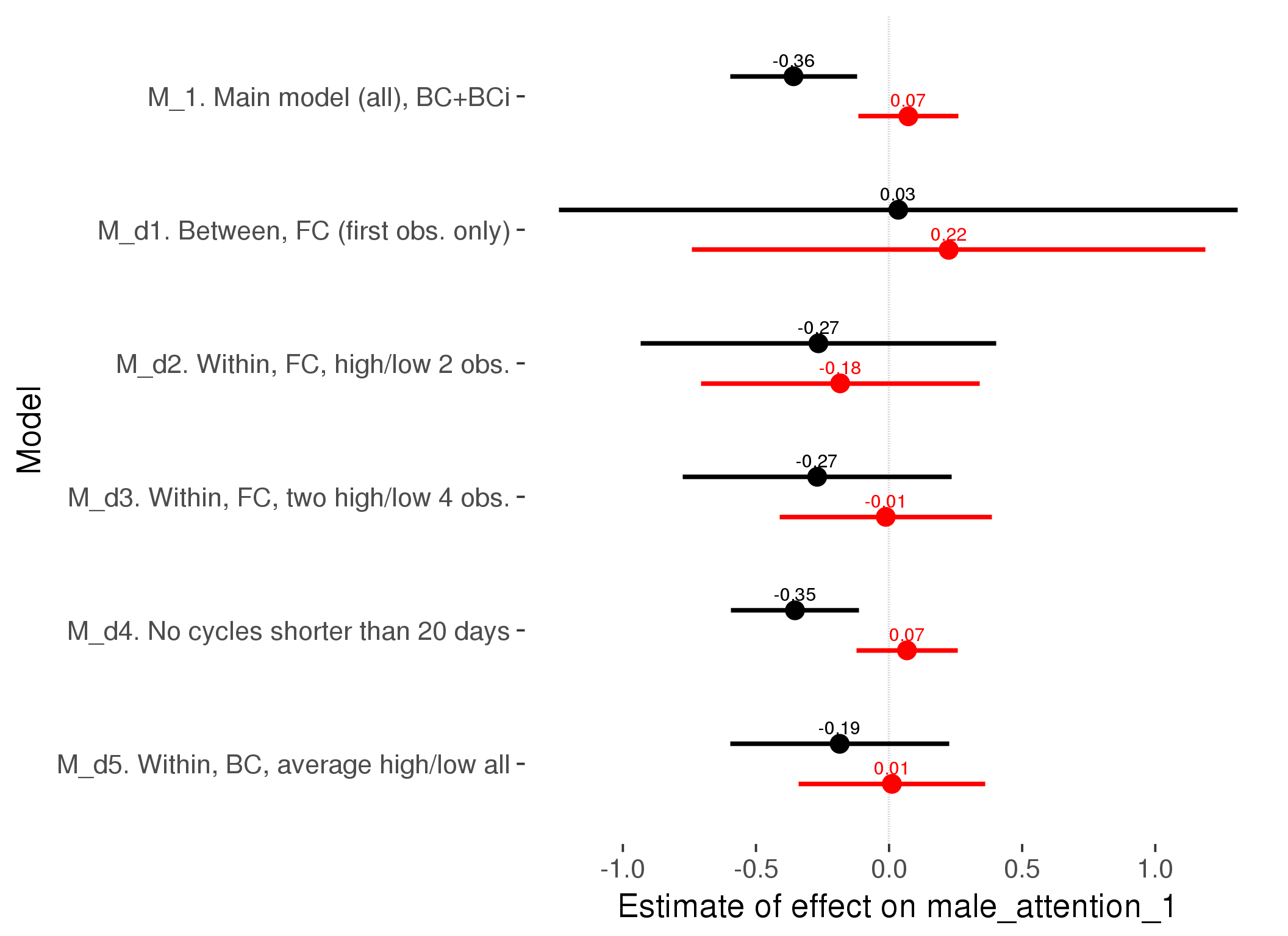
M_m1: Moderation by contraceptive method
Based on the sample with lax exclusion criteria. Users who used any hormonal contraception are classified as hormonal, users who use any awareness-based methods (counting, temperature-based) are classified as ‘fertility-awareness’, women who don’t fall into the before groups and use condoms, pessars, coitus interruptus etc. are classified as ‘barrie or abstinence’. Women who don’t use contraception or use other methods such as sterilisation are excluded from this analysis.
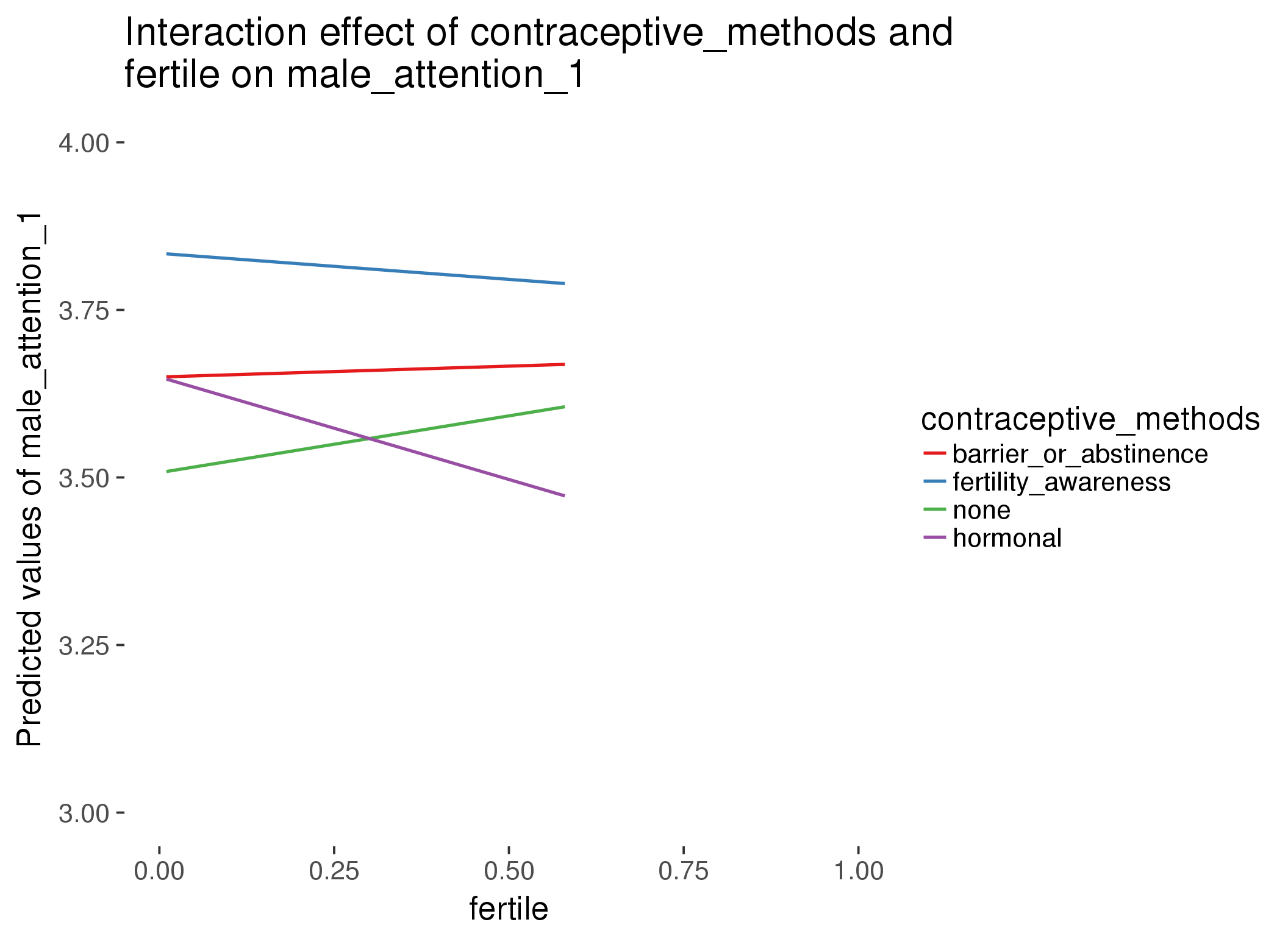
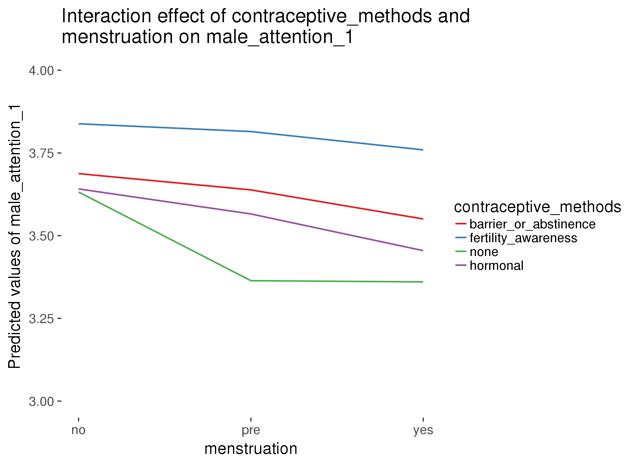
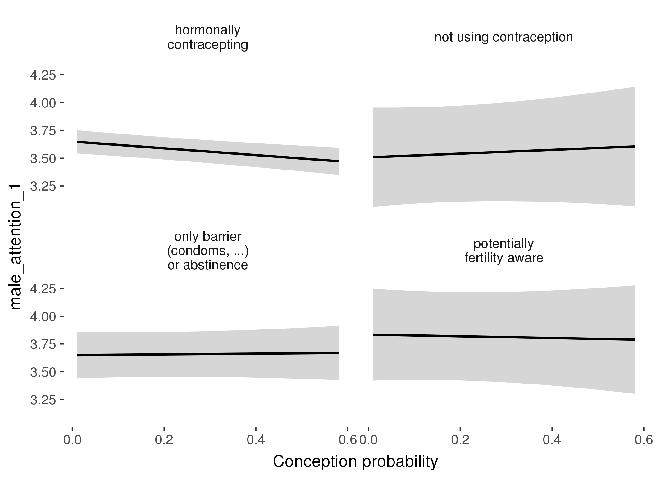
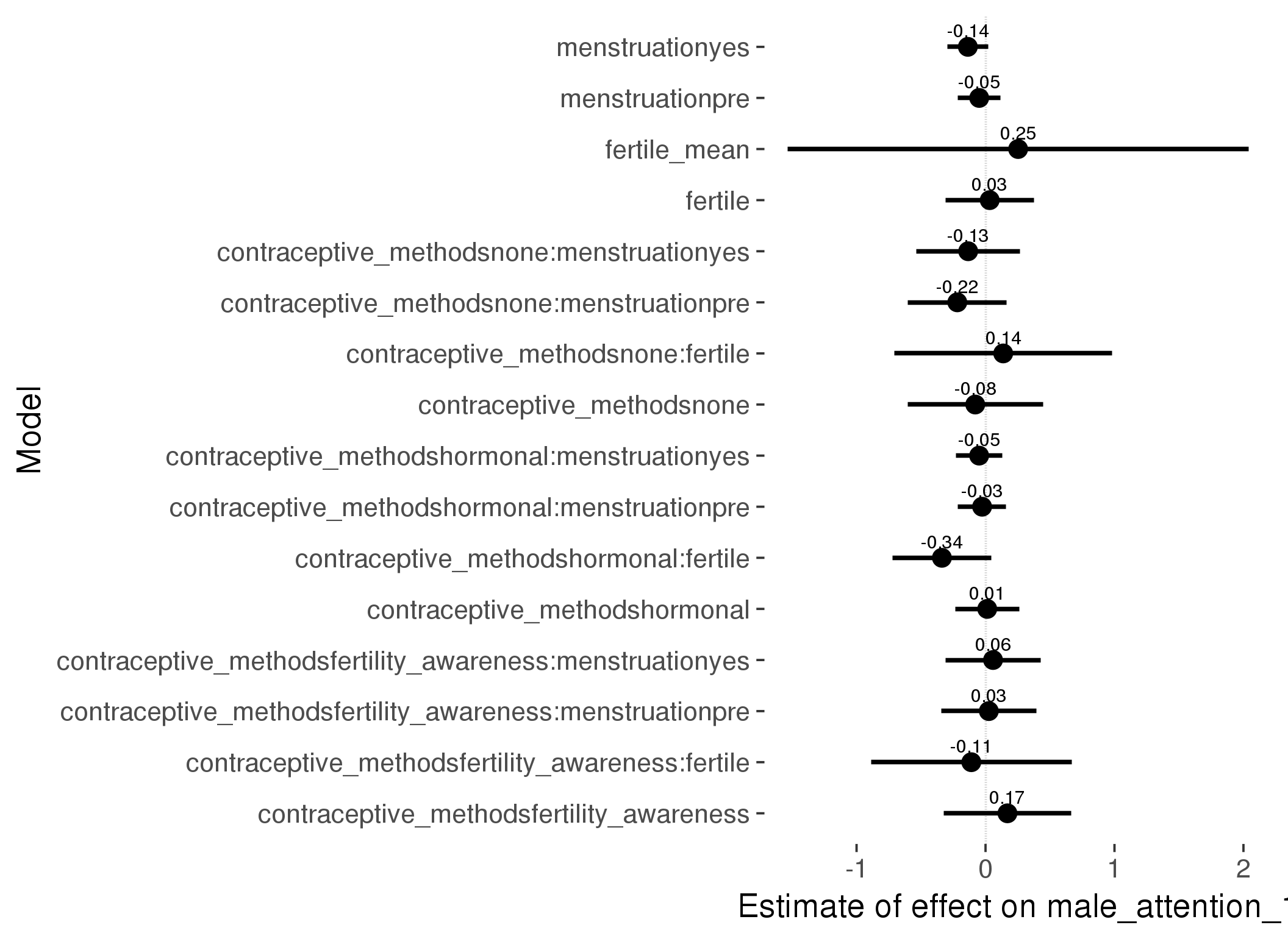
Linear mixed model fit by REML ['lmerMod']
Formula: male_attention_1 ~ fertile_mean + (1 | person) + contraceptive_methods +
fertile + menstruation + fertile:contraceptive_methods + menstruation:contraceptive_methods
Data: diary
Subset: !is.na(included_lax) & contraceptive_method != "other"
REML criterion at convergence: 65006
Scaled residuals:
Min 1Q Median 3Q Max
-2.881 -0.734 0.005 0.724 2.853
Random effects:
Groups Name Variance Std.Dev.
person (Intercept) 0.905 0.951
Residual 2.464 1.570
Number of obs: 17026, groups: person, 513
Fixed effects:
Estimate Std. Error t value
(Intercept) 3.6375 0.1893 19.22
fertile_mean 0.2528 0.9124 0.28
contraceptive_methodsfertility_awareness 0.1701 0.2527 0.67
contraceptive_methodsnone -0.0796 0.2680 -0.30
contraceptive_methodshormonal 0.0131 0.1271 0.10
fertile 0.0324 0.1749 0.19
menstruationpre -0.0491 0.0845 -0.58
menstruationyes -0.1371 0.0807 -1.70
contraceptive_methodsfertility_awareness:fertile -0.1101 0.3973 -0.28
contraceptive_methodsnone:fertile 0.1370 0.4303 0.32
contraceptive_methodshormonal:fertile -0.3382 0.1954 -1.73
contraceptive_methodsfertility_awareness:menstruationpre 0.0256 0.1873 0.14
contraceptive_methodsnone:menstruationpre -0.2189 0.1957 -1.12
contraceptive_methodshormonal:menstruationpre -0.0266 0.0952 -0.28
contraceptive_methodsfertility_awareness:menstruationyes 0.0582 0.1882 0.31
contraceptive_methodsnone:menstruationyes -0.1345 0.2047 -0.66
contraceptive_methodshormonal:menstruationyes -0.0495 0.0920 -0.54
refitting model(s) with ML (instead of REML)
| Df | AIC | BIC | logLik | deviance | Chisq | Chi Df | Pr(>Chisq) | |
|---|---|---|---|---|---|---|---|---|
| add_main | 13 | 64998 | 65099 | -32486 | 64972 | NA | NA | NA |
| by_method | 19 | 65007 | 65154 | -32485 | 64969 | 3.253 | 6 | 0.7765 |
M_m2: Moderation by participant age
model %>%
test_moderator("age_group", diary, xlevels = 5)refitting model(s) with ML (instead of REML)
| Df | AIC | BIC | logLik | deviance | Chisq | Chi Df | Pr(>Chisq) | |
|---|---|---|---|---|---|---|---|---|
| with_main | 19 | 101950 | 102105 | -50956 | 101912 | NA | NA | NA |
| with_mod | 27 | 101955 | 102176 | -50950 | 101901 | 10.94 | 8 | 0.2049 |
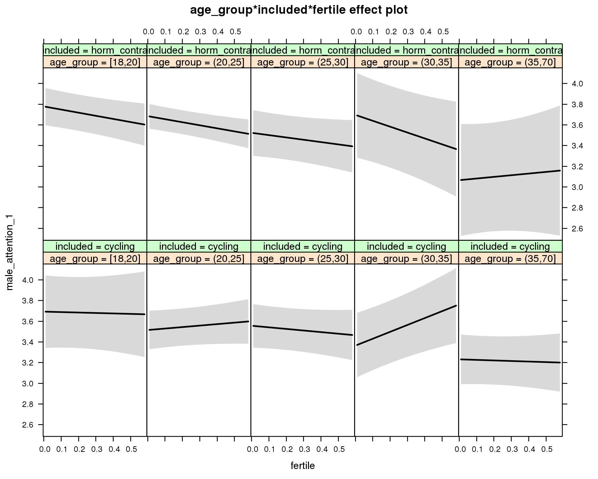
Linear mixed model fit by REML ['lmerMod']
Formula: male_attention_1 ~ menstruation + fertile_mean + (1 | person) +
age_group + included + fertile + menstruation:included +
age_group:included + age_group:fertile + included:fertile + age_group:included:fertile
Data: diary
REML criterion at convergence: 101957
Scaled residuals:
Min 1Q Median 3Q Max
-2.9036 -0.7335 -0.0045 0.7190 2.8662
Random effects:
Groups Name Variance Std.Dev.
person (Intercept) 0.994 0.997
Residual 2.446 1.564
Number of obs: 26680, groups: person, 1054
Fixed effects:
Estimate Std. Error t value
(Intercept) 3.733344 0.190584 19.59
menstruationpre -0.053990 0.047659 -1.13
menstruationyes -0.174314 0.044897 -3.88
fertile_mean -0.004578 0.430278 -0.01
age_group(20,25] -0.177890 0.202600 -0.88
age_group(25,30] -0.136349 0.208619 -0.65
age_group(30,35] -0.328738 0.239345 -1.37
age_group(35,70] -0.461226 0.216710 -2.13
includedhorm_contra 0.093290 0.203420 0.46
fertile -0.043688 0.275078 -0.16
menstruationpre:includedhorm_contra -0.042641 0.061190 -0.70
menstruationyes:includedhorm_contra -0.000882 0.058863 -0.01
age_group(20,25]:includedhorm_contra 0.084166 0.230747 0.36
age_group(25,30]:includedhorm_contra -0.118634 0.254485 -0.47
age_group(30,35]:includedhorm_contra 0.246762 0.330820 0.75
age_group(35,70]:includedhorm_contra -0.251755 0.363937 -0.69
age_group(20,25]:fertile 0.186634 0.304620 0.61
age_group(25,30]:fertile -0.110424 0.314011 -0.35
age_group(30,35]:fertile 0.710563 0.363598 1.95
age_group(35,70]:fertile -0.009863 0.328197 -0.03
includedhorm_contra:fertile -0.258540 0.305079 -0.85
age_group(20,25]:includedhorm_contra:fertile -0.179361 0.341246 -0.53
age_group(25,30]:includedhorm_contra:fertile 0.188169 0.378093 0.50
age_group(30,35]:includedhorm_contra:fertile -0.977596 0.487842 -2.00
age_group(35,70]:includedhorm_contra:fertile 0.471683 0.554571 0.85
M_m3: Moderation by weekend
model %>%
test_moderator("weekend", diary, xlevels = 2) refitting model(s) with ML (instead of REML)
| Df | AIC | BIC | logLik | deviance | Chisq | Chi Df | Pr(>Chisq) | |
|---|---|---|---|---|---|---|---|---|
| with_main | 13 | 101617 | 101723 | -50795 | 101591 | NA | NA | NA |
| with_mod | 15 | 101618 | 101741 | -50794 | 101588 | 2.706 | 2 | 0.2584 |
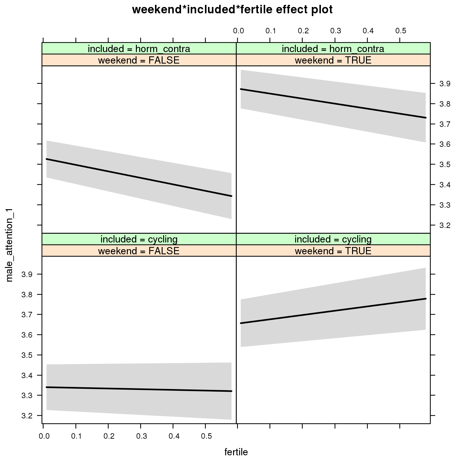
Linear mixed model fit by REML ['lmerMod']
Formula: male_attention_1 ~ menstruation + fertile_mean + (1 | person) +
weekend + included + fertile + menstruation:included + weekend:included +
weekend:fertile + included:fertile + weekend:included:fertile
Data: diary
REML criterion at convergence: 101636
Scaled residuals:
Min 1Q Median 3Q Max
-3.0397 -0.7365 0.0025 0.7095 2.9397
Random effects:
Groups Name Variance Std.Dev.
person (Intercept) 1.00 1.00
Residual 2.41 1.55
Number of obs: 26680, groups: person, 1054
Fixed effects:
Estimate Std. Error t value
(Intercept) 3.37663 0.09435 35.8
menstruationpre -0.05204 0.04734 -1.1
menstruationyes -0.17394 0.04458 -3.9
fertile_mean 0.02021 0.42864 0.0
weekendTRUE 0.31428 0.04131 7.6
includedhorm_contra 0.19600 0.07895 2.5
fertile -0.03393 0.11628 -0.3
menstruationpre:includedhorm_contra -0.04504 0.06078 -0.7
menstruationyes:includedhorm_contra 0.00507 0.05846 0.1
weekendTRUE:includedhorm_contra 0.03094 0.05318 0.6
weekendTRUE:fertile 0.24647 0.16022 1.5
includedhorm_contra:fertile -0.28802 0.14767 -2.0
weekendTRUE:includedhorm_contra:fertile -0.17309 0.20381 -0.8
M_m4: Moderation by weekday
model %>%
test_moderator("weekday", diary, xlevels = 7)refitting model(s) with ML (instead of REML)
| Df | AIC | BIC | logLik | deviance | Chisq | Chi Df | Pr(>Chisq) | |
|---|---|---|---|---|---|---|---|---|
| with_main | 23 | 101406 | 101594 | -50680 | 101360 | NA | NA | NA |
| with_mod | 35 | 101415 | 101702 | -50673 | 101345 | 14.71 | 12 | 0.2578 |
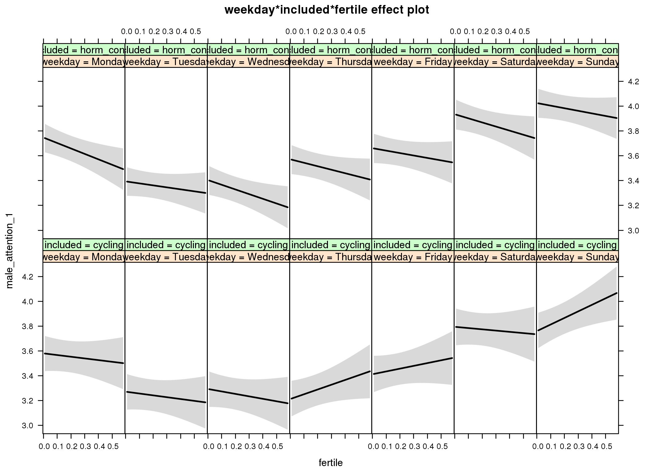
Linear mixed model fit by REML ['lmerMod']
Formula: male_attention_1 ~ menstruation + fertile_mean + (1 | person) +
weekday + included + fertile + menstruation:included + weekday:included +
weekday:fertile + included:fertile + weekday:included:fertile
Data: diary
REML criterion at convergence: 101447
Scaled residuals:
Min 1Q Median 3Q Max
-3.0592 -0.7272 0.0084 0.7121 3.0130
Random effects:
Groups Name Variance Std.Dev.
person (Intercept) 1.00 1.00
Residual 2.39 1.55
Number of obs: 26680, groups: person, 1054
Fixed effects:
Estimate Std. Error t value
(Intercept) 3.62169 0.10443 34.7
menstruationpre -0.05292 0.04715 -1.1
menstruationyes -0.17561 0.04440 -4.0
fertile_mean -0.00744 0.42841 0.0
weekdayTuesday -0.30886 0.07363 -4.2
weekdayWednesday -0.28706 0.07350 -3.9
weekdayThursday -0.36823 0.07434 -5.0
weekdayFriday -0.16823 0.07560 -2.2
weekdaySaturday 0.21385 0.07634 2.8
weekdaySunday 0.17966 0.07379 2.4
includedhorm_contra 0.17219 0.09753 1.8
fertile -0.13611 0.20732 -0.7
menstruationpre:includedhorm_contra -0.04144 0.06053 -0.7
menstruationyes:includedhorm_contra 0.00974 0.05821 0.2
weekdayTuesday:includedhorm_contra -0.04432 0.09459 -0.5
weekdayWednesday:includedhorm_contra -0.05558 0.09490 -0.6
weekdayThursday:includedhorm_contra 0.19326 0.09581 2.0
weekdayFriday:includedhorm_contra 0.08268 0.09712 0.9
weekdaySaturday:includedhorm_contra -0.02598 0.09824 -0.3
weekdaySunday:includedhorm_contra 0.09832 0.09525 1.0
weekdayTuesday:fertile -0.01192 0.28540 0.0
weekdayWednesday:fertile -0.06238 0.28675 -0.2
weekdayThursday:fertile 0.52097 0.29084 1.8
weekdayFriday:fertile 0.36067 0.29138 1.2
weekdaySaturday:fertile 0.03457 0.29526 0.1
weekdaySunday:fertile 0.66385 0.28693 2.3
includedhorm_contra:fertile -0.30238 0.26513 -1.1
weekdayTuesday:includedhorm_contra:fertile 0.29020 0.36429 0.8
weekdayWednesday:includedhorm_contra:fertile 0.12347 0.36716 0.3
weekdayThursday:includedhorm_contra:fertile -0.36344 0.37017 -1.0
weekdayFriday:includedhorm_contra:fertile -0.11905 0.37131 -0.3
weekdaySaturday:includedhorm_contra:fertile 0.07347 0.37666 0.2
weekdaySunday:includedhorm_contra:fertile -0.43350 0.36654 -1.2
M_m5: Moderation by exclusion threshold
model %>%
test_moderator("included_levels", diary, xlevels = 4)refitting model(s) with ML (instead of REML)
| Df | AIC | BIC | logLik | deviance | Chisq | Chi Df | Pr(>Chisq) | |
|---|---|---|---|---|---|---|---|---|
| with_main | 17 | 101946 | 102086 | -50956 | 101912 | NA | NA | NA |
| with_mod | 23 | 101955 | 102143 | -50955 | 101909 | 3.25 | 6 | 0.7769 |
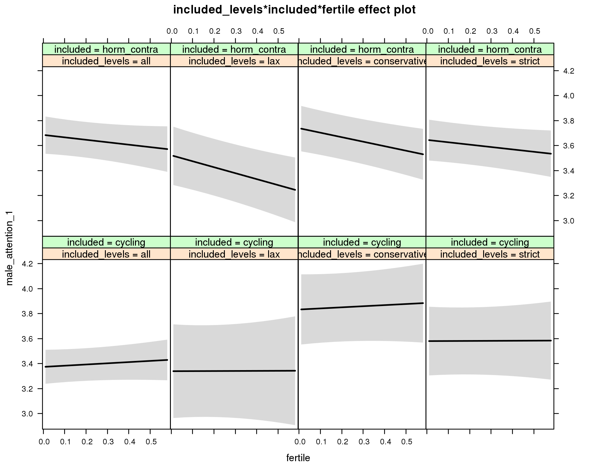
Linear mixed model fit by REML ['lmerMod']
Formula: male_attention_1 ~ menstruation + fertile_mean + (1 | person) +
included_levels + included + fertile + menstruation:included +
included_levels:included + included_levels:fertile + included:fertile +
included_levels:included:fertile
Data: diary
REML criterion at convergence: 101964
Scaled residuals:
Min 1Q Median 3Q Max
-2.8752 -0.7333 -0.0033 0.7178 2.9113
Random effects:
Groups Name Variance Std.Dev.
person (Intercept) 0.989 0.995
Residual 2.447 1.564
Number of obs: 26680, groups: person, 1054
Fixed effects:
Estimate Std. Error t value
(Intercept) 3.41664 0.10279 33.2
menstruationpre -0.05497 0.04770 -1.2
menstruationyes -0.17212 0.04489 -3.8
fertile_mean -0.01859 0.43274 0.0
included_levelslax -0.03441 0.20358 -0.2
included_levelsconservative 0.45895 0.15908 2.9
included_levelsstrict 0.20631 0.15642 1.3
includedhorm_contra 0.31884 0.10619 3.0
fertile 0.09574 0.12148 0.8
menstruationpre:includedhorm_contra -0.03994 0.06126 -0.7
menstruationyes:includedhorm_contra -0.00266 0.05891 0.0
included_levelslax:includedhorm_contra -0.12865 0.24850 -0.5
included_levelsconservative:includedhorm_contra -0.40539 0.19942 -2.0
included_levelsstrict:includedhorm_contra -0.24623 0.19298 -1.3
included_levelslax:fertile -0.08964 0.29713 -0.3
included_levelsconservative:fertile -0.00764 0.22179 0.0
included_levelsstrict:fertile -0.08871 0.22196 -0.4
includedhorm_contra:fertile -0.29130 0.18508 -1.6
included_levelslax:includedhorm_contra:fertile -0.19159 0.36230 -0.5
included_levelsconservative:includedhorm_contra:fertile -0.15638 0.28813 -0.5
included_levelsstrict:includedhorm_contra:fertile 0.09412 0.28367 0.3
M_m6: Moderation by cycle length
model %>%
test_moderator("cycle_length_groups", diary, xlevels = 4)refitting model(s) with ML (instead of REML)
| Df | AIC | BIC | logLik | deviance | Chisq | Chi Df | Pr(>Chisq) | |
|---|---|---|---|---|---|---|---|---|
| with_main | 17 | 101951 | 102090 | -50958 | 101917 | NA | NA | NA |
| with_mod | 23 | 101958 | 102147 | -50956 | 101912 | 4.368 | 6 | 0.627 |
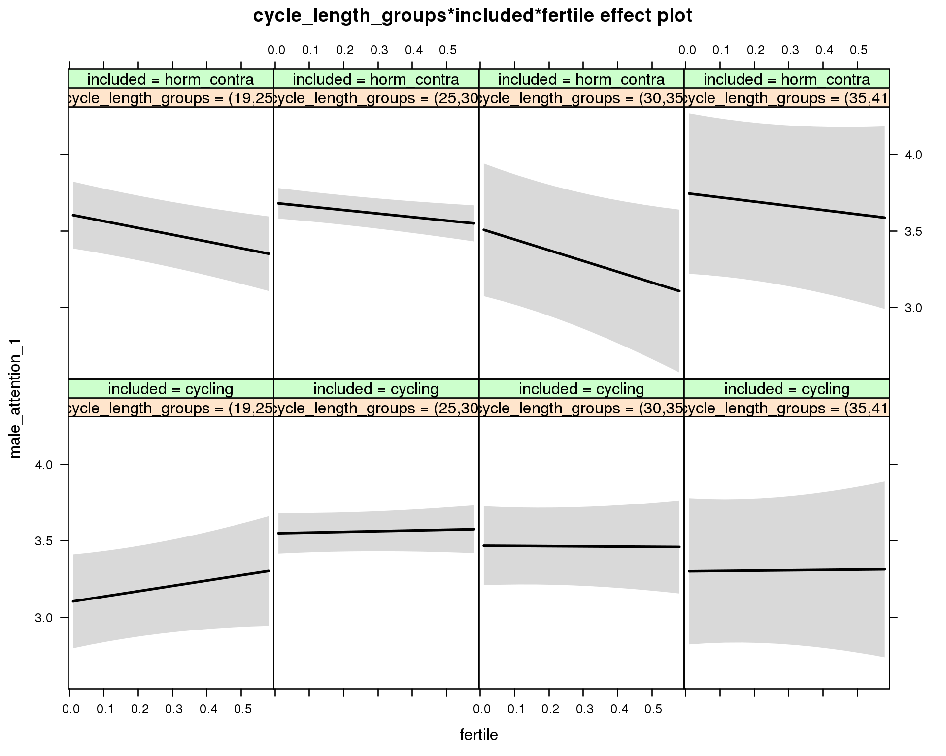
Linear mixed model fit by REML ['lmerMod']
Formula: male_attention_1 ~ menstruation + fertile_mean + (1 | person) +
cycle_length_groups + included + fertile + menstruation:included +
cycle_length_groups:included + cycle_length_groups:fertile +
included:fertile + cycle_length_groups:included:fertile
Data: diary
REML criterion at convergence: 101959
Scaled residuals:
Min 1Q Median 3Q Max
-2.8876 -0.7325 -0.0046 0.7168 2.8569
Random effects:
Groups Name Variance Std.Dev.
person (Intercept) 0.996 0.998
Residual 2.447 1.564
Number of obs: 26680, groups: person, 1054
Fixed effects:
Estimate Std. Error t value
(Intercept) 3.14960 0.17485 18.01
menstruationpre -0.05410 0.04772 -1.13
menstruationyes -0.17769 0.04521 -3.93
fertile_mean -0.04919 0.43413 -0.11
cycle_length_groups(25,30] 0.44822 0.17096 2.62
cycle_length_groups(30,35] 0.36720 0.20507 1.79
cycle_length_groups(35,41] 0.19956 0.29044 0.69
includedhorm_contra 0.51195 0.19452 2.63
fertile 0.34787 0.25363 1.37
menstruationpre:includedhorm_contra -0.03855 0.06124 -0.63
menstruationyes:includedhorm_contra 0.00946 0.05919 0.16
cycle_length_groups(25,30]:includedhorm_contra -0.37359 0.21055 -1.77
cycle_length_groups(30,35]:includedhorm_contra -0.46079 0.32181 -1.43
cycle_length_groups(35,41]:includedhorm_contra -0.06051 0.41037 -0.15
cycle_length_groups(25,30]:fertile -0.30154 0.27210 -1.11
cycle_length_groups(30,35]:fertile -0.36206 0.32228 -1.12
cycle_length_groups(35,41]:fertile -0.32544 0.45523 -0.71
includedhorm_contra:fertile -0.79031 0.29948 -2.64
cycle_length_groups(25,30]:includedhorm_contra:fertile 0.51437 0.32247 1.60
cycle_length_groups(30,35]:includedhorm_contra:fertile 0.10229 0.50766 0.20
cycle_length_groups(35,41]:includedhorm_contra:fertile 0.49203 0.59966 0.82
M_m7: Moderation by certainty about menstruation parameters
model %>%
test_moderator("certainty_menstruation", diary)refitting model(s) with ML (instead of REML)
| Df | AIC | BIC | logLik | deviance | Chisq | Chi Df | Pr(>Chisq) | |
|---|---|---|---|---|---|---|---|---|
| with_main | 13 | 101943 | 102050 | -50959 | 101917 | NA | NA | NA |
| with_mod | 15 | 101938 | 102061 | -50954 | 101908 | 8.673 | 2 | 0.01308 |
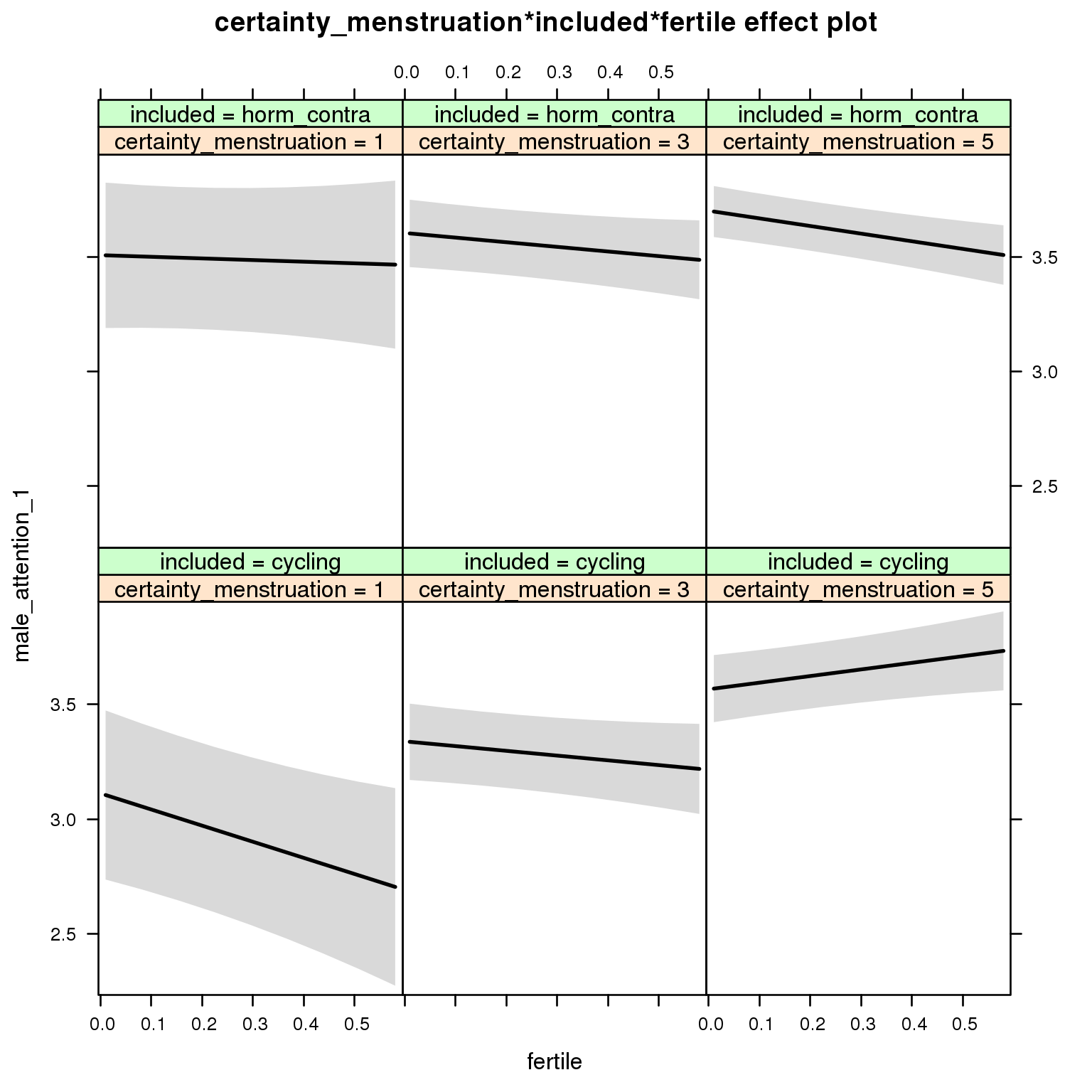
Linear mixed model fit by REML ['lmerMod']
Formula: male_attention_1 ~ menstruation + fertile_mean + (1 | person) +
certainty_menstruation + included + fertile + menstruation:included +
certainty_menstruation:included + certainty_menstruation:fertile +
included:fertile + certainty_menstruation:included:fertile
Data: diary
REML criterion at convergence: 101957
Scaled residuals:
Min 1Q Median 3Q Max
-2.8808 -0.7339 -0.0027 0.7191 2.8688
Random effects:
Groups Name Variance Std.Dev.
person (Intercept) 0.99 0.995
Residual 2.45 1.564
Number of obs: 26680, groups: person, 1054
Fixed effects:
Estimate Std. Error t value
(Intercept) 3.04278 0.25401 11.98
menstruationpre -0.04758 0.04767 -1.00
menstruationyes -0.16459 0.04493 -3.66
fertile_mean -0.04056 0.42878 -0.09
certainty_menstruation 0.11358 0.05782 1.96
includedhorm_contra 0.47048 0.32227 1.46
fertile -0.95128 0.37836 -2.51
menstruationpre:includedhorm_contra -0.04681 0.06119 -0.76
menstruationyes:includedhorm_contra -0.00963 0.05888 -0.16
certainty_menstruation:includedhorm_contra -0.06518 0.07496 -0.87
certainty_menstruation:fertile 0.24801 0.08865 2.80
includedhorm_contra:fertile 0.94544 0.49170 1.92
certainty_menstruation:includedhorm_contra:fertile -0.31337 0.11365 -2.76
M_m8: Moderation by cycle regularity
model %>%
test_moderator("cycle_regularity", diary)refitting model(s) with ML (instead of REML)
| Df | AIC | BIC | logLik | deviance | Chisq | Chi Df | Pr(>Chisq) | |
|---|---|---|---|---|---|---|---|---|
| with_main | 15 | 101952 | 102075 | -50961 | 101922 | NA | NA | NA |
| with_mod | 19 | 101957 | 102112 | -50959 | 101919 | 3.514 | 4 | 0.4757 |
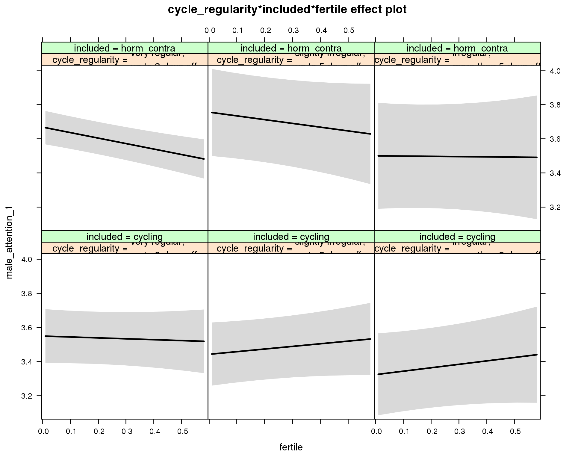
Linear mixed model fit by REML ['lmerMod']
Formula: male_attention_1 ~ menstruation + fertile_mean + (1 | person) +
cycle_regularity + included + fertile + menstruation:included +
cycle_regularity:included + cycle_regularity:fertile + included:fertile +
cycle_regularity:included:fertile
Data: diary
REML criterion at convergence: 101966
Scaled residuals:
Min 1Q Median 3Q Max
-2.8790 -0.7339 -0.0027 0.7170 2.8595
Random effects:
Groups Name Variance Std.Dev.
person (Intercept) 1.00 1.00
Residual 2.45 1.56
Number of obs: 26680, groups: person, 1054
Fixed effects:
Estimate Std. Error t value
(Intercept) 3.59046 0.10935 32.8
menstruationpre -0.05462 0.04769 -1.1
menstruationyes -0.17304 0.04489 -3.9
fertile_mean -0.00717 0.43141 0.0
cycle_regularityslightly irregular,\nup to 5 days off -0.10691 0.12415 -0.9
cycle_regularityirregular,\nmore than 5 days off -0.22615 0.14676 -1.5
includedhorm_contra 0.12719 0.09898 1.3
fertile -0.05291 0.13316 -0.4
menstruationpre:includedhorm_contra -0.04071 0.06121 -0.7
menstruationyes:includedhorm_contra -0.00204 0.05886 0.0
cycle_regularityslightly irregular,\nup to 5 days off:includedhorm_contra 0.19492 0.18720 1.0
cycle_regularityirregular,\nmore than 5 days off:includedhorm_contra 0.05781 0.22198 0.3
cycle_regularityslightly irregular,\nup to 5 days off:fertile 0.20748 0.18358 1.1
cycle_regularityirregular,\nmore than 5 days off:fertile 0.25426 0.22566 1.1
includedhorm_contra:fertile -0.26899 0.15596 -1.7
cycle_regularityslightly irregular,\nup to 5 days off:includedhorm_contra:fertile -0.10602 0.27272 -0.4
cycle_regularityirregular,\nmore than 5 days off:includedhorm_contra:fertile 0.05220 0.33689 0.2
M_m9: Moderation by cohabitation status
model %>%
test_moderator("cohabitation", diary)refitting model(s) with ML (instead of REML)
| Df | AIC | BIC | logLik | deviance | Chisq | Chi Df | Pr(>Chisq) | |
|---|---|---|---|---|---|---|---|---|
| with_main | 15 | 101936 | 102058 | -50953 | 101906 | NA | NA | NA |
| with_mod | 19 | 101942 | 102097 | -50952 | 101904 | 1.977 | 4 | 0.74 |
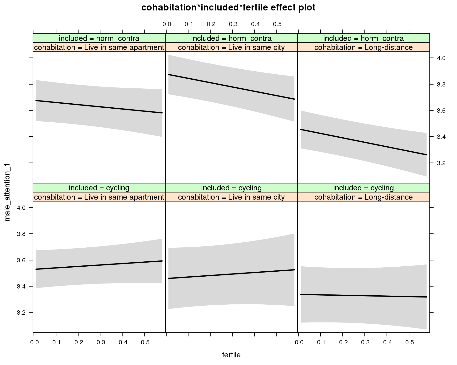
Linear mixed model fit by REML ['lmerMod']
Formula: male_attention_1 ~ menstruation + fertile_mean + (1 | person) +
cohabitation + included + fertile + menstruation:included +
cohabitation:included + cohabitation:fertile + included:fertile + cohabitation:included:fertile
Data: diary
REML criterion at convergence: 101954
Scaled residuals:
Min 1Q Median 3Q Max
-2.8674 -0.7322 -0.0037 0.7187 2.8858
Random effects:
Groups Name Variance Std.Dev.
person (Intercept) 0.979 0.99
Residual 2.447 1.56
Number of obs: 26680, groups: person, 1054
Fixed effects:
Estimate Std. Error t value
(Intercept) 3.58122 0.10511 34.1
menstruationpre -0.05130 0.04765 -1.1
menstruationyes -0.17046 0.04488 -3.8
fertile_mean -0.07818 0.42732 -0.2
cohabitationLive in same city -0.07036 0.14001 -0.5
cohabitationLong-distance -0.19136 0.13197 -1.5
includedhorm_contra 0.15590 0.11189 1.4
fertile 0.10996 0.12022 0.9
menstruationpre:includedhorm_contra -0.04364 0.06118 -0.7
menstruationyes:includedhorm_contra -0.00239 0.05884 0.0
cohabitationLive in same city:includedhorm_contra 0.27085 0.17881 1.5
cohabitationLong-distance:includedhorm_contra -0.02711 0.17103 -0.2
cohabitationLive in same city:fertile 0.00516 0.21942 0.0
cohabitationLong-distance:fertile -0.14313 0.19768 -0.7
includedhorm_contra:fertile -0.27467 0.17553 -1.6
cohabitationLive in same city:includedhorm_contra:fertile -0.16980 0.27442 -0.6
cohabitationLong-distance:includedhorm_contra:fertile -0.03133 0.25472 -0.1
M_m10: Moderation by relationship status
model %>%
test_moderator("relationship_status_clean", diary)refitting model(s) with ML (instead of REML)
| Df | AIC | BIC | logLik | deviance | Chisq | Chi Df | Pr(>Chisq) | |
|---|---|---|---|---|---|---|---|---|
| with_main | 15 | 101947 | 102070 | -50958 | 101917 | NA | NA | NA |
| with_mod | 19 | 101952 | 102108 | -50957 | 101914 | 2.721 | 4 | 0.6055 |
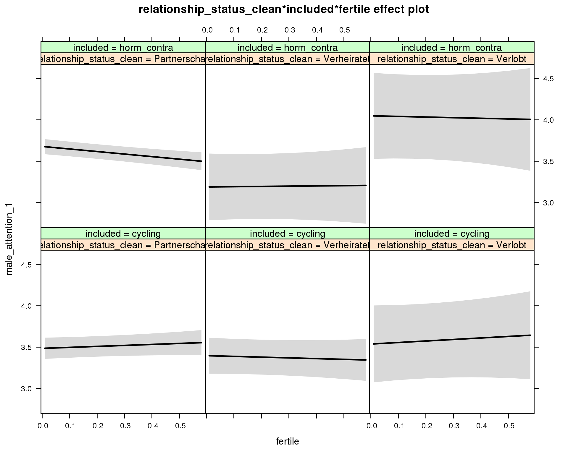
Linear mixed model fit by REML ['lmerMod']
Formula: male_attention_1 ~ menstruation + fertile_mean + (1 | person) +
relationship_status_clean + included + fertile + menstruation:included +
relationship_status_clean:included + relationship_status_clean:fertile +
included:fertile + relationship_status_clean:included:fertile
Data: diary
REML criterion at convergence: 101955
Scaled residuals:
Min 1Q Median 3Q Max
-2.8664 -0.7337 -0.0016 0.7216 2.8714
Random effects:
Groups Name Variance Std.Dev.
person (Intercept) 0.993 0.997
Residual 2.447 1.564
Number of obs: 26680, groups: person, 1054
Fixed effects:
Estimate Std. Error t value
(Intercept) 3.5231 0.0989 35.6
menstruationpre -0.0519 0.0476 -1.1
menstruationyes -0.1715 0.0449 -3.8
fertile_mean 0.0148 0.4290 0.0
relationship_status_cleanVerheiratet -0.0881 0.1287 -0.7
relationship_status_cleanVerlobt 0.0525 0.2465 0.2
includedhorm_contra 0.1996 0.0847 2.4
fertile 0.1193 0.1101 1.1
menstruationpre:includedhorm_contra -0.0436 0.0612 -0.7
menstruationyes:includedhorm_contra -0.0026 0.0588 0.0
relationship_status_cleanVerheiratet:includedhorm_contra -0.4015 0.2477 -1.6
relationship_status_cleanVerlobt:includedhorm_contra 0.3178 0.3655 0.9
relationship_status_cleanVerheiratet:fertile -0.2087 0.1938 -1.1
relationship_status_cleanVerlobt:fertile 0.0637 0.3633 0.2
includedhorm_contra:fertile -0.4276 0.1341 -3.2
relationship_status_cleanVerheiratet:includedhorm_contra:fertile 0.5481 0.3650 1.5
relationship_status_cleanVerlobt:includedhorm_contra:fertile 0.1696 0.5645 0.3
In-pair public intimacy
model_summaries$in_pair_public_intimacyModel summary
Model summary
model %>%
print_summary()Generalized linear mixed model fit by maximum likelihood (Laplace Approximation) ['glmerMod']
Family: binomial ( probit )
Formula: in_pair_public_intimacy ~ included * (menstruation + fertile) + fertile_mean + (1 | person)
Data: diary
AIC BIC logLik deviance df.resid
33038 33120 -16509 33018 26694
Scaled residuals:
Min 1Q Median 3Q Max
-3.837 -0.782 -0.355 0.859 3.973
Random effects:
Groups Name Variance Std.Dev.
person (Intercept) 0.484 0.695
Number of obs: 26704, groups: person, 1054
Fixed effects:
Estimate Std. Error z value Pr(>|z|)
(Intercept) -0.08872 0.07023 -1.26 0.207
includedhorm_contra 0.00403 0.05720 0.07 0.944
menstruationpre -0.03489 0.04124 -0.85 0.398
menstruationyes 0.02872 0.03904 0.74 0.462
fertile -0.12896 0.08349 -1.54 0.122
fertile_mean 0.15231 0.32707 0.47 0.641
includedhorm_contra:menstruationpre -0.02417 0.05279 -0.46 0.647
includedhorm_contra:menstruationyes -0.10312 0.05108 -2.02 0.043 *
includedhorm_contra:fertile -0.13970 0.10543 -1.32 0.185
---
Signif. codes: 0 '***' 0.001 '**' 0.01 '*' 0.05 '.' 0.1 ' ' 1
Correlation of Fixed Effects:
(Intr) incld_ mnstrtnp mnstrtny fertil frtl_m inclddhrm_cntr:mnstrtnp
inclddhrm_c -0.472
menstrutnpr -0.233 0.291
menstrutnys -0.223 0.277 0.391
fertile -0.220 0.356 0.466 0.379
fertile_men -0.772 -0.032 -0.006 -0.003 -0.088
inclddhrm_cntr:mnstrtnp 0.190 -0.364 -0.781 -0.305 -0.363 -0.007
inclddhrm_cntr:mnstrtny 0.178 -0.339 -0.299 -0.764 -0.289 -0.008 0.378
inclddhrm_cntr:f 0.219 -0.450 -0.369 -0.300 -0.787 0.012 0.466
inclddhrm_cntr:mnstrtny
inclddhrm_c
menstrutnpr
menstrutnys
fertile
fertile_men
inclddhrm_cntr:mnstrtnp
inclddhrm_cntr:mnstrtny
inclddhrm_cntr:f 0.377
convergence code: 0
Model failed to converge with max|grad| = 0.00118339 (tol = 0.001, component 1)
Effect size standardised by residual variance (\(\frac{b}{ SD_{residual} }\)): -0.13 [-0.29;0.03].
Marginal effect plots
model %>%
plot_all_effects()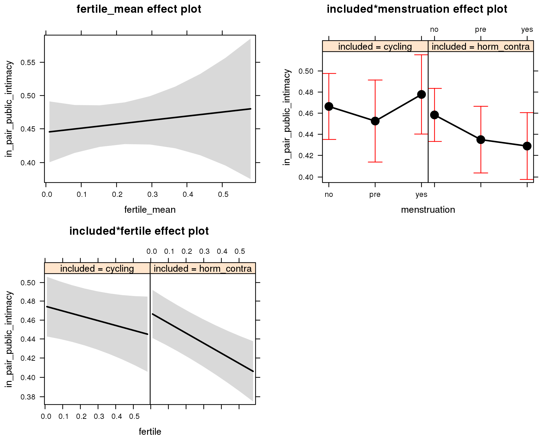
Outcome distribution
model %>%
plot_outcome(diary) + xlab(outcome_label)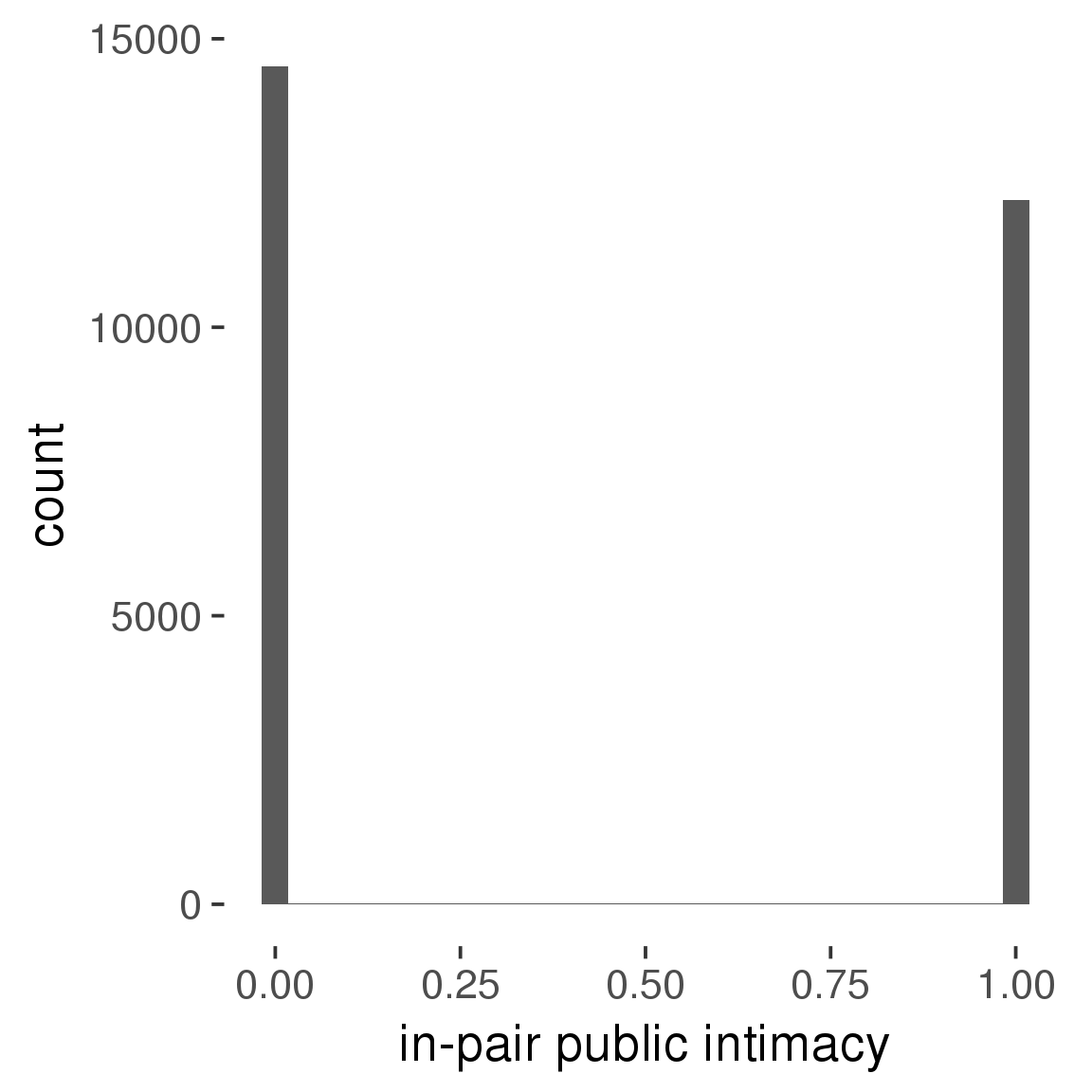
Diagnostics
model %>%
print_diagnostics()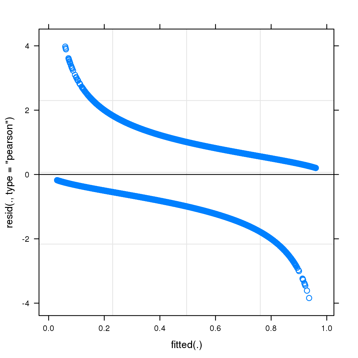
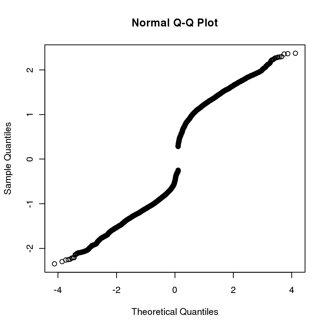
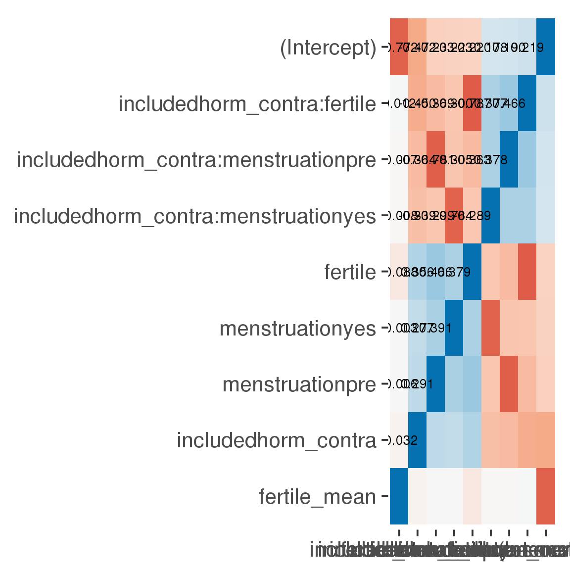
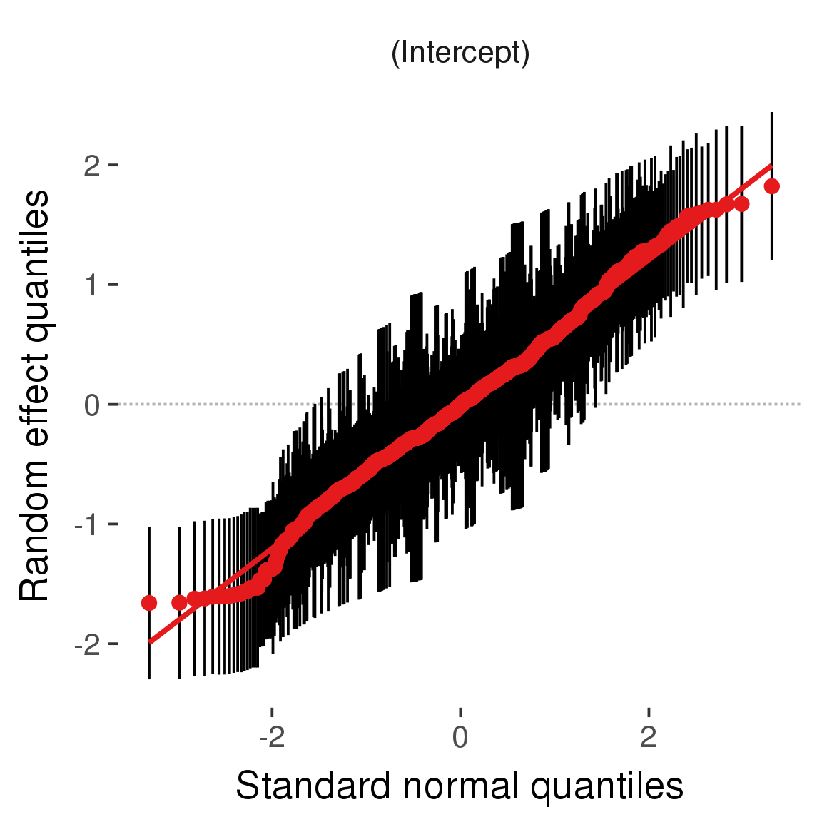
Curves
Here, we continuously plot the outcome over the course of the cycle. Because cycle lengths vary, we subset the data to cycles in a certain range. If the red curve traces the pink curve, our predictor accurately maps the relationship between fertile window probability and the outcome.
Cycle lengths from 21 to 36
Backward-counted
model %>%
plot_curve(diary %>% filter(minimum_cycle_length_diary <= 36, minimum_cycle_length_diary > 20) %>% mutate(fertile=prc_stirn_b))outcome = names(model@frame)[1]
outcome_label = recode(str_replace_all(str_replace_all(str_replace_all(outcome, "_", " "), " pair", "-pair"), " 1", ""),
"desirability 1" = "self-perceived desirability",
"NARQ admiration" = "narcissistic admiration",
"NARQ rivalry" = "narcissistic rivalry",
"extra-pair" = "extra-pair desire & behaviour",
"had sexual intercourse" = "sexual intercourse")
library(ggplot2)
# form a subset and run the model without the hormonal contraception and the fertility predictors
tmp = diary %>%
filter(!is.na(fertile), !is.na(included),
RCD > -1 * minimum_cycle_length_diary, RCD > -40)
new_form = update.formula(formula(model), new = . ~ . - fertile * included)
tmp$residuals = residuals(update(model, new_form, data = tmp , na.action = na.exclude))
tmp = tmp %>%
filter(!is.na(RCD), !is.na(residuals))
rcd_min = min(tmp$RCD)
tmp$real = FALSE
tmp_before = tmp
tmp_before$RCD = tmp_before$RCD + min(tmp$RCD) - 1
tmp_after = tmp
tmp_after$RCD = tmp_after$RCD - min(tmp$RCD) + 1
tmp$real = TRUE
tmp = bind_rows(tmp_before %>% filter(RCD > rcd_min - 11), tmp, tmp_after %>% filter(RCD < 11))GAM smooth on residuals
Here, we partialled out menstruation and individual random effects, then superimposed estimated probability of being in the fertile window scaled to the range of the estimated means. To address the periodicity of the cycle, we prepended and appended ten days of the timeseries to the end and the beginning of the timeseries. We then estimated the GAM and cut off the appended subsets before plotting.
tryCatch({
trend_plot = ggplot(tmp,aes(x = RCD, y = residuals, colour = included)) +
stat_smooth(geom = 'smooth',size = 0.8, fill = "#9ECAE1", method = 'gam', formula = y ~ s(x))
}, error = function(e){cat_message(e, "danger")})
tryCatch({
trend_data = ggplot_build(trend_plot)$data[[1]]
}, error = function(e){cat_message(e, "danger")})
trend_data$RCD = round(trend_data$x)
trend_data = left_join(trend_data, tmp %>% select(real, RCD,fertile) %>% unique(), by = "RCD")
trend_data %>%
filter(real == TRUE) %>%
mutate(superimposed = ( ( (fertile - 0.01)/0.58) * (max(y)-min(y) ) ) + min(y) ) ->
trend_data
ggplot(trend_data) +
geom_ribbon(aes(x = x, ymin = ymin, ymax = ymax, fill = factor(group)), alpha = 0.2) +
geom_line(aes(x = x, y = y, colour = factor(group)), size = 0.8, stat = "identity") +
scale_x_continuous(caption_x) +
geom_line(aes(x = x, y = superimposed), color = "#a83fbf", size = 1, linetype = 'dashed') +
annotate("text",x = mean(trend_data$x), y = max(trend_data$superimposed,na.rm=T) + 0.1, label = 'superimposed fertility peak', color = "#a83fbf") +
scale_y_continuous(outcome_label) +
ggtitle("GAM smooth, residuals") +
scale_color_manual("Contraception status",values = c("2"="black","1"= "red"), labels = c("2"="hormonally\ncontracepting","1"="cycling"), guide = F) +
scale_fill_manual("Contraception status",values = c("2"="black","1"= "red"), labels = c("2"="hormonally\ncontracepting","1"="cycling"), guide = F)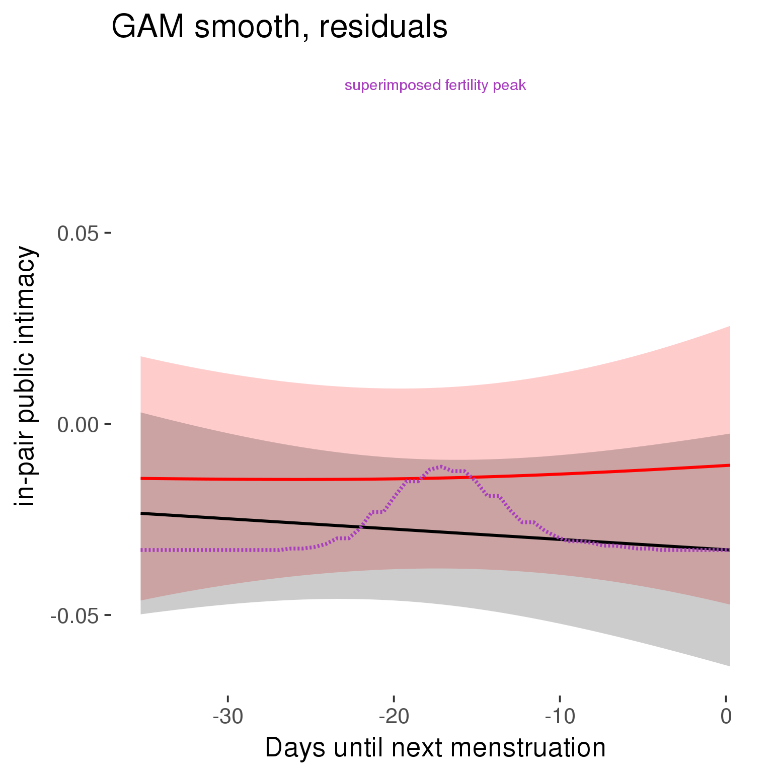
GAM smooth on raw data
As before, but without partialling anything out.
tryCatch({
trend_plot = ggplot(tmp,aes_string(x = "RCD", y = outcome, colour = "included")) +
stat_smooth(geom = 'smooth',size = 0.8, fill = "#9ECAE1", method = 'gam', formula = y ~ s(x))
}, error = function(e){cat_message(e, "danger")})
tryCatch({
trend_data = ggplot_build(trend_plot)$data[[1]]
}, error = function(e){cat_message(e, "danger")})
trend_data$RCD = round(trend_data$x)
trend_data = left_join(trend_data, tmp %>% select(real, RCD,fertile) %>% unique(), by = "RCD")
trend_data %>%
filter(real == TRUE) %>%
mutate(superimposed = ( ( (fertile - 0.01)/0.58) * (max(y)-min(y) ) ) + min(y) ) ->
trend_data
plot1b = ggplot(trend_data) +
geom_ribbon(aes(x = x, ymin = ymin, ymax = ymax, fill = factor(group)), alpha = 0.2) +
geom_line(aes(x = x, y = y, colour = factor(group)), size = 0.8, stat = "identity") +
scale_x_continuous(caption_x) +
geom_line(aes(x = x, y = superimposed), color = "#a83fbf", size = 1, linetype = 'dashed') +
annotate("text",x = mean(trend_data$x), y = max(trend_data$superimposed,na.rm=T) + 0.1, label = 'superimposed fertility peak', color = "#a83fbf") +
scale_y_continuous(outcome_label) +
ggtitle("GAM smooth, raw data") +
scale_color_manual("Contraception status",values = c("2"="black","1"= "red"), labels = c("2"="hormonally\ncontracepting","1"="cycling"), guide = F) +
scale_fill_manual("Contraception status",values = c("2"="black","1"= "red"), labels = c("2"="hormonally\ncontracepting","1"="cycling"), guide = F)
suppressWarnings(print(plot1b))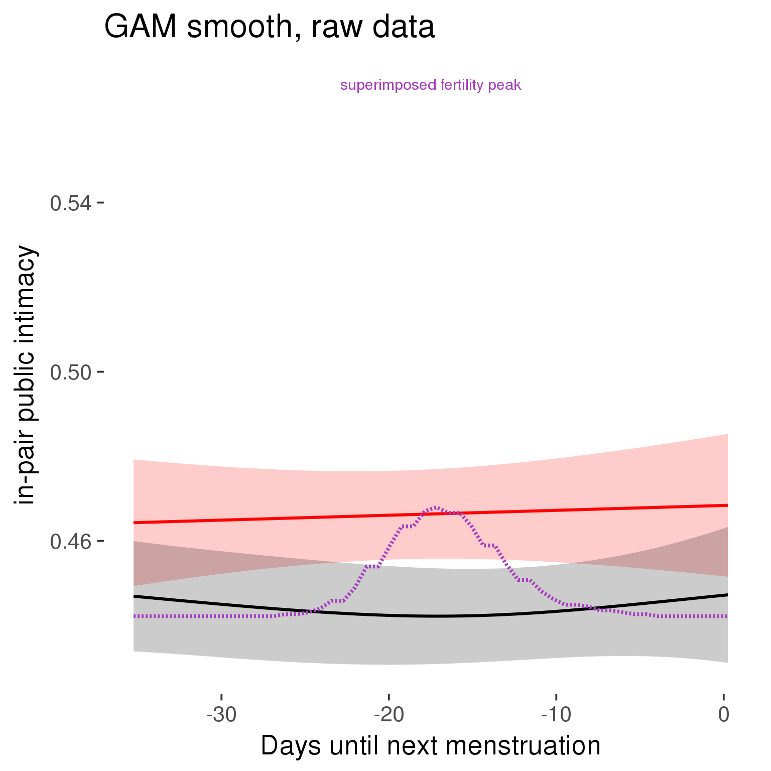
Means and standard errors over raw data
Nothing partialled out, just straight means with bootstrapped confidence intervals.
tryCatch({
trend_plot = ggplot(tmp,aes_string(x = "RCD", y = outcome, colour = "included")) +
geom_pointrange(size = 0.8, stat = 'summary', fun.data = "mean_cl_boot")
}, error = function(e){cat_message(e, "danger")})
tryCatch({
trend_data = ggplot_build(trend_plot)$data[[1]]
}, error = function(e){cat_message(e, "danger")})
trend_data$RCD = round(trend_data$x)
trend_data = left_join(trend_data, tmp %>% select(real, RCD,fertile) %>% unique(), by = "RCD")
trend_data %>%
filter(real == TRUE) %>%
mutate(superimposed = ( ( (fertile - 0.01)/0.58) * (max(y)-min(y) ) ) + min(y) ) ->
trend_data
plot3 = ggplot(trend_data) +
geom_pointrange(aes(x = x, y = y, ymin = ymin,ymax = ymax, colour = factor(group)), size = 0.8, stat = "identity", alpha = 0.6, position = position_dodge(width = .5)) +
scale_x_continuous("Days until next menstruation") +
geom_line(aes(x= x, y = superimposed), color = "#a83fbf", size = 1, linetype = 'dashed') +
annotate("text",x = mean(trend_data$x), y = max(trend_data$superimposed,na.rm=T) + 0.1, label = 'superimposed fertility peak', color = "#a83fbf") +
scale_y_continuous(outcome_label) +
ggtitle("Means with standard errors, raw data") +
scale_color_manual("Contraception status",values = c("2"="black","1"= "red"), labels = c("2"="hormonally\ncontracepting","1"="cycling"), guide = F) +
scale_fill_manual("Contraception status",values = c("2"="black","1"= "red"), labels = c("2"="hormonally\ncontracepting","1"="cycling"), guide = F)
suppressWarnings(print(plot3))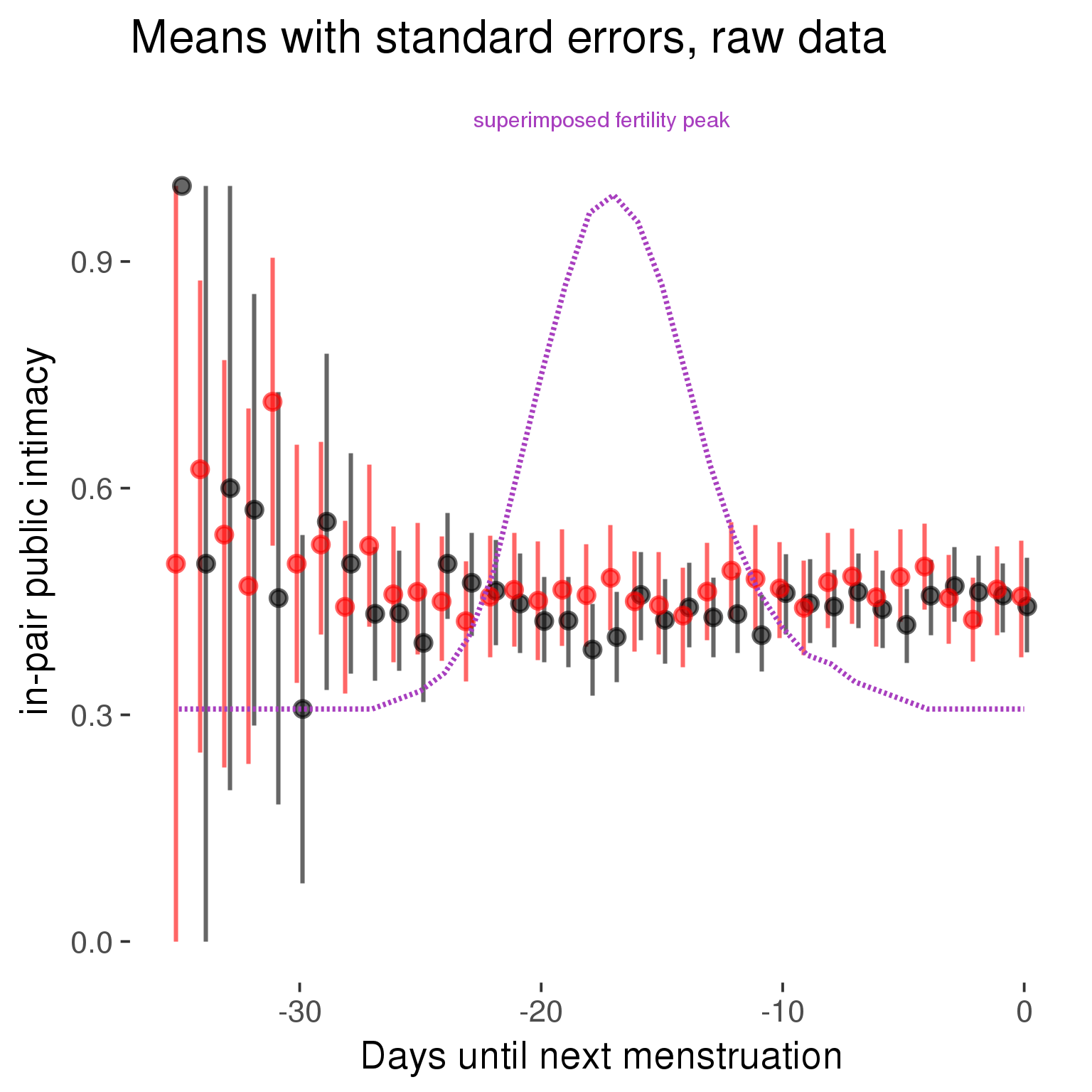
Forward-counted
model %>%
plot_curve(diary %>% filter(minimum_cycle_length_diary <= 36, minimum_cycle_length_diary > 20) %>% mutate(RCD = FCD, fertile = prc_stirn_b_forward_counted), caption_x = "Days since last menstruation")outcome = names(model@frame)[1]
outcome_label = recode(str_replace_all(str_replace_all(str_replace_all(outcome, "_", " "), " pair", "-pair"), " 1", ""),
"desirability 1" = "self-perceived desirability",
"NARQ admiration" = "narcissistic admiration",
"NARQ rivalry" = "narcissistic rivalry",
"extra-pair" = "extra-pair desire & behaviour",
"had sexual intercourse" = "sexual intercourse")
library(ggplot2)
# form a subset and run the model without the hormonal contraception and the fertility predictors
tmp = diary %>%
filter(!is.na(fertile), !is.na(included),
RCD > -1 * minimum_cycle_length_diary, RCD > -40)
new_form = update.formula(formula(model), new = . ~ . - fertile * included)
tmp$residuals = residuals(update(model, new_form, data = tmp , na.action = na.exclude))
tmp = tmp %>%
filter(!is.na(RCD), !is.na(residuals))
rcd_min = min(tmp$RCD)
tmp$real = FALSE
tmp_before = tmp
tmp_before$RCD = tmp_before$RCD + min(tmp$RCD) - 1
tmp_after = tmp
tmp_after$RCD = tmp_after$RCD - min(tmp$RCD) + 1
tmp$real = TRUE
tmp = bind_rows(tmp_before %>% filter(RCD > rcd_min - 11), tmp, tmp_after %>% filter(RCD < 11))GAM smooth on residuals
Here, we partialled out menstruation and individual random effects, then superimposed estimated probability of being in the fertile window scaled to the range of the estimated means. To address the periodicity of the cycle, we prepended and appended ten days of the timeseries to the end and the beginning of the timeseries. We then estimated the GAM and cut off the appended subsets before plotting.
tryCatch({
trend_plot = ggplot(tmp,aes(x = RCD, y = residuals, colour = included)) +
stat_smooth(geom = 'smooth',size = 0.8, fill = "#9ECAE1", method = 'gam', formula = y ~ s(x))
}, error = function(e){cat_message(e, "danger")})
tryCatch({
trend_data = ggplot_build(trend_plot)$data[[1]]
}, error = function(e){cat_message(e, "danger")})
trend_data$RCD = round(trend_data$x)
trend_data = left_join(trend_data, tmp %>% select(real, RCD,fertile) %>% unique(), by = "RCD")
trend_data %>%
filter(real == TRUE) %>%
mutate(superimposed = ( ( (fertile - 0.01)/0.58) * (max(y)-min(y) ) ) + min(y) ) ->
trend_data
ggplot(trend_data) +
geom_ribbon(aes(x = x, ymin = ymin, ymax = ymax, fill = factor(group)), alpha = 0.2) +
geom_line(aes(x = x, y = y, colour = factor(group)), size = 0.8, stat = "identity") +
scale_x_continuous(caption_x) +
geom_line(aes(x = x, y = superimposed), color = "#a83fbf", size = 1, linetype = 'dashed') +
annotate("text",x = mean(trend_data$x), y = max(trend_data$superimposed,na.rm=T) + 0.1, label = 'superimposed fertility peak', color = "#a83fbf") +
scale_y_continuous(outcome_label) +
ggtitle("GAM smooth, residuals") +
scale_color_manual("Contraception status",values = c("2"="black","1"= "red"), labels = c("2"="hormonally\ncontracepting","1"="cycling"), guide = F) +
scale_fill_manual("Contraception status",values = c("2"="black","1"= "red"), labels = c("2"="hormonally\ncontracepting","1"="cycling"), guide = F)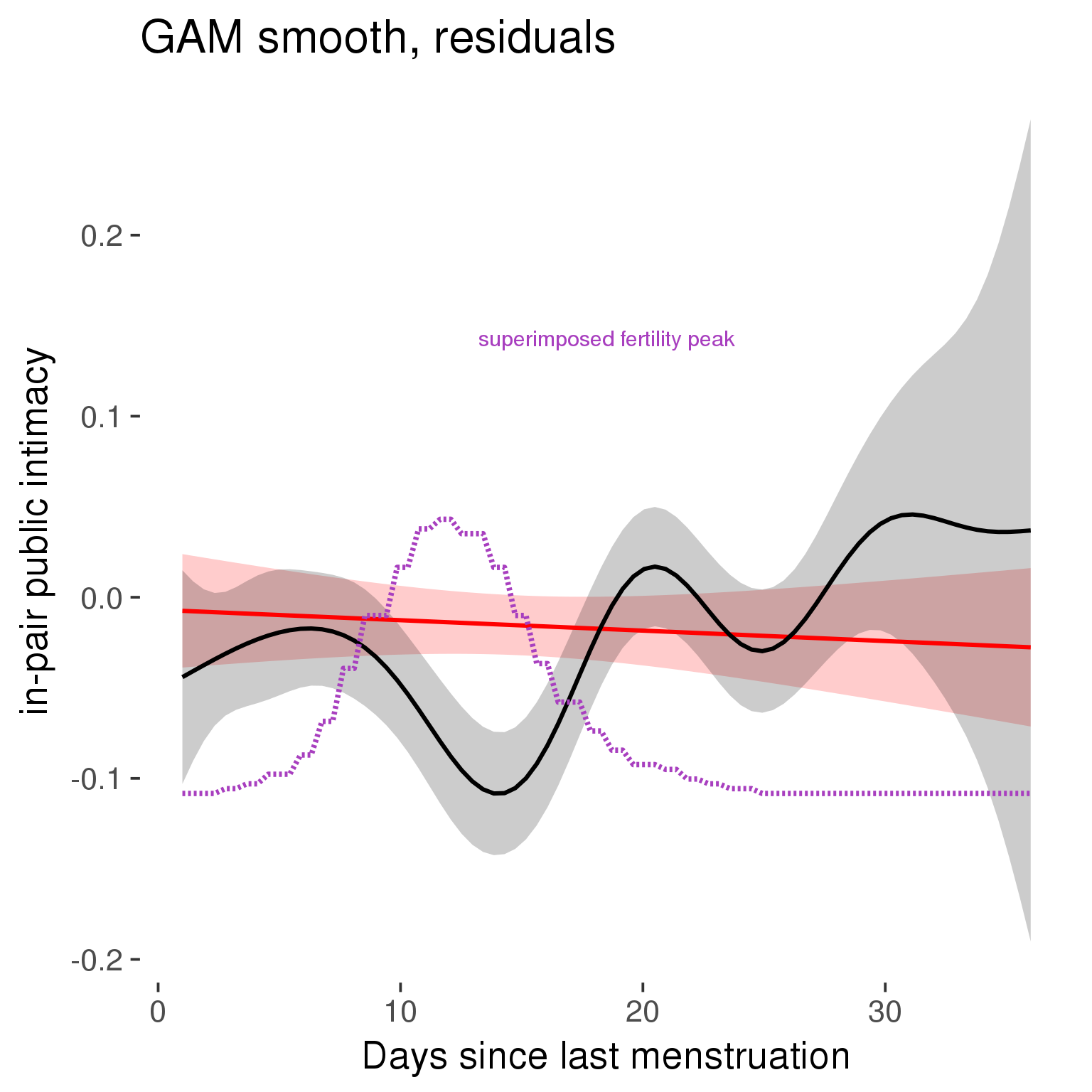
GAM smooth on raw data
As before, but without partialling anything out.
tryCatch({
trend_plot = ggplot(tmp,aes_string(x = "RCD", y = outcome, colour = "included")) +
stat_smooth(geom = 'smooth',size = 0.8, fill = "#9ECAE1", method = 'gam', formula = y ~ s(x))
}, error = function(e){cat_message(e, "danger")})
tryCatch({
trend_data = ggplot_build(trend_plot)$data[[1]]
}, error = function(e){cat_message(e, "danger")})
trend_data$RCD = round(trend_data$x)
trend_data = left_join(trend_data, tmp %>% select(real, RCD,fertile) %>% unique(), by = "RCD")
trend_data %>%
filter(real == TRUE) %>%
mutate(superimposed = ( ( (fertile - 0.01)/0.58) * (max(y)-min(y) ) ) + min(y) ) ->
trend_data
plot1b = ggplot(trend_data) +
geom_ribbon(aes(x = x, ymin = ymin, ymax = ymax, fill = factor(group)), alpha = 0.2) +
geom_line(aes(x = x, y = y, colour = factor(group)), size = 0.8, stat = "identity") +
scale_x_continuous(caption_x) +
geom_line(aes(x = x, y = superimposed), color = "#a83fbf", size = 1, linetype = 'dashed') +
annotate("text",x = mean(trend_data$x), y = max(trend_data$superimposed,na.rm=T) + 0.1, label = 'superimposed fertility peak', color = "#a83fbf") +
scale_y_continuous(outcome_label) +
ggtitle("GAM smooth, raw data") +
scale_color_manual("Contraception status",values = c("2"="black","1"= "red"), labels = c("2"="hormonally\ncontracepting","1"="cycling"), guide = F) +
scale_fill_manual("Contraception status",values = c("2"="black","1"= "red"), labels = c("2"="hormonally\ncontracepting","1"="cycling"), guide = F)
suppressWarnings(print(plot1b))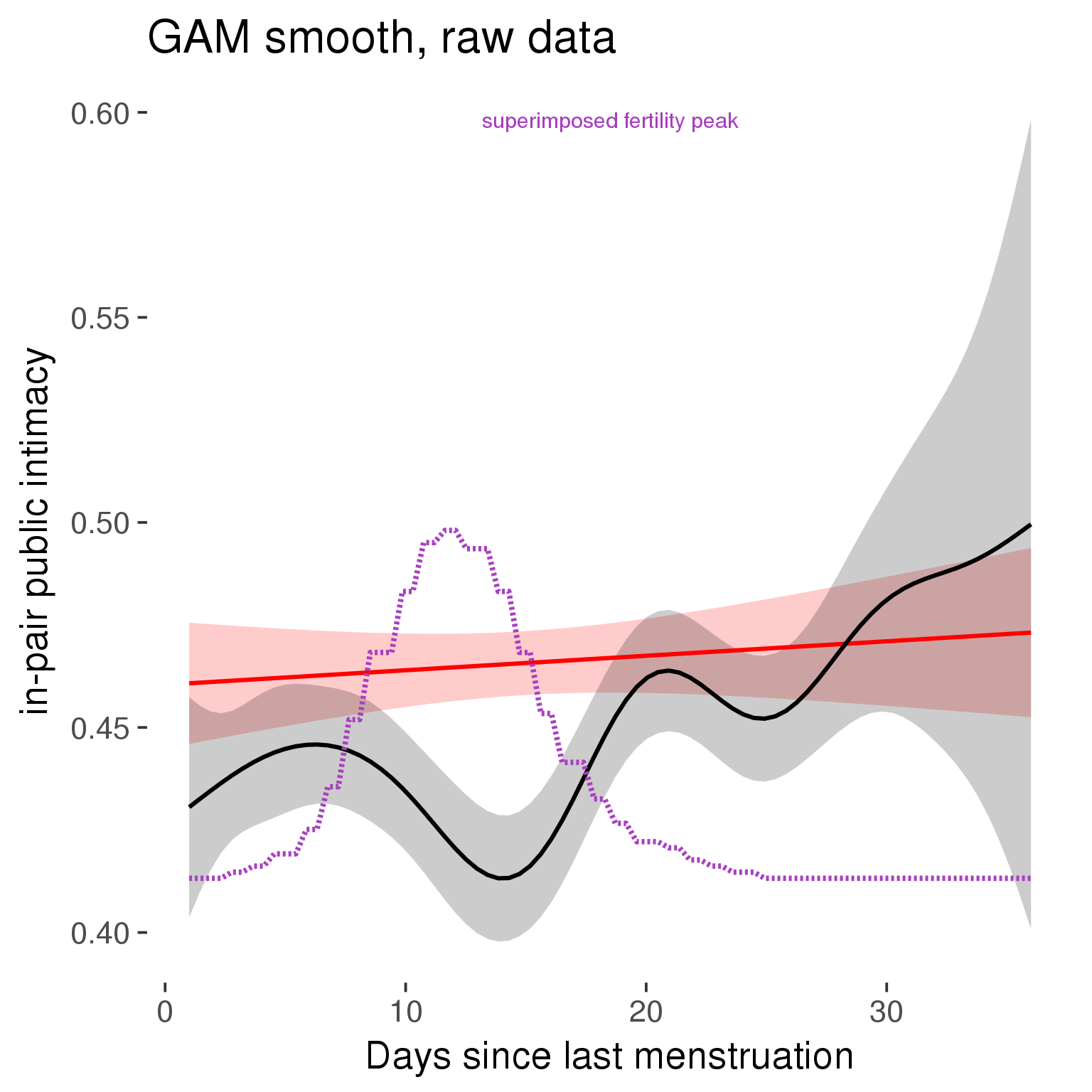
Means and standard errors over raw data
Nothing partialled out, just straight means with bootstrapped confidence intervals.
tryCatch({
trend_plot = ggplot(tmp,aes_string(x = "RCD", y = outcome, colour = "included")) +
geom_pointrange(size = 0.8, stat = 'summary', fun.data = "mean_cl_boot")
}, error = function(e){cat_message(e, "danger")})
tryCatch({
trend_data = ggplot_build(trend_plot)$data[[1]]
}, error = function(e){cat_message(e, "danger")})
trend_data$RCD = round(trend_data$x)
trend_data = left_join(trend_data, tmp %>% select(real, RCD,fertile) %>% unique(), by = "RCD")
trend_data %>%
filter(real == TRUE) %>%
mutate(superimposed = ( ( (fertile - 0.01)/0.58) * (max(y)-min(y) ) ) + min(y) ) ->
trend_data
plot3 = ggplot(trend_data) +
geom_pointrange(aes(x = x, y = y, ymin = ymin,ymax = ymax, colour = factor(group)), size = 0.8, stat = "identity", alpha = 0.6, position = position_dodge(width = .5)) +
scale_x_continuous("Days until next menstruation") +
geom_line(aes(x= x, y = superimposed), color = "#a83fbf", size = 1, linetype = 'dashed') +
annotate("text",x = mean(trend_data$x), y = max(trend_data$superimposed,na.rm=T) + 0.1, label = 'superimposed fertility peak', color = "#a83fbf") +
scale_y_continuous(outcome_label) +
ggtitle("Means with standard errors, raw data") +
scale_color_manual("Contraception status",values = c("2"="black","1"= "red"), labels = c("2"="hormonally\ncontracepting","1"="cycling"), guide = F) +
scale_fill_manual("Contraception status",values = c("2"="black","1"= "red"), labels = c("2"="hormonally\ncontracepting","1"="cycling"), guide = F)
suppressWarnings(print(plot3))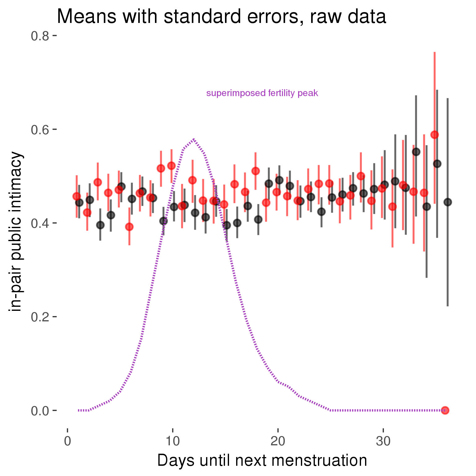
Cycle lengths from 27 to 30
Backward-counted
model %>%
plot_curve(diary %>% filter(minimum_cycle_length_diary <= 30, minimum_cycle_length_diary >= 27) %>% mutate(fertile=prc_stirn_b))outcome = names(model@frame)[1]
outcome_label = recode(str_replace_all(str_replace_all(str_replace_all(outcome, "_", " "), " pair", "-pair"), " 1", ""),
"desirability 1" = "self-perceived desirability",
"NARQ admiration" = "narcissistic admiration",
"NARQ rivalry" = "narcissistic rivalry",
"extra-pair" = "extra-pair desire & behaviour",
"had sexual intercourse" = "sexual intercourse")
library(ggplot2)
# form a subset and run the model without the hormonal contraception and the fertility predictors
tmp = diary %>%
filter(!is.na(fertile), !is.na(included),
RCD > -1 * minimum_cycle_length_diary, RCD > -40)
new_form = update.formula(formula(model), new = . ~ . - fertile * included)
tmp$residuals = residuals(update(model, new_form, data = tmp , na.action = na.exclude))
tmp = tmp %>%
filter(!is.na(RCD), !is.na(residuals))
rcd_min = min(tmp$RCD)
tmp$real = FALSE
tmp_before = tmp
tmp_before$RCD = tmp_before$RCD + min(tmp$RCD) - 1
tmp_after = tmp
tmp_after$RCD = tmp_after$RCD - min(tmp$RCD) + 1
tmp$real = TRUE
tmp = bind_rows(tmp_before %>% filter(RCD > rcd_min - 11), tmp, tmp_after %>% filter(RCD < 11))GAM smooth on residuals
Here, we partialled out menstruation and individual random effects, then superimposed estimated probability of being in the fertile window scaled to the range of the estimated means. To address the periodicity of the cycle, we prepended and appended ten days of the timeseries to the end and the beginning of the timeseries. We then estimated the GAM and cut off the appended subsets before plotting.
tryCatch({
trend_plot = ggplot(tmp,aes(x = RCD, y = residuals, colour = included)) +
stat_smooth(geom = 'smooth',size = 0.8, fill = "#9ECAE1", method = 'gam', formula = y ~ s(x))
}, error = function(e){cat_message(e, "danger")})
tryCatch({
trend_data = ggplot_build(trend_plot)$data[[1]]
}, error = function(e){cat_message(e, "danger")})
trend_data$RCD = round(trend_data$x)
trend_data = left_join(trend_data, tmp %>% select(real, RCD,fertile) %>% unique(), by = "RCD")
trend_data %>%
filter(real == TRUE) %>%
mutate(superimposed = ( ( (fertile - 0.01)/0.58) * (max(y)-min(y) ) ) + min(y) ) ->
trend_data
ggplot(trend_data) +
geom_ribbon(aes(x = x, ymin = ymin, ymax = ymax, fill = factor(group)), alpha = 0.2) +
geom_line(aes(x = x, y = y, colour = factor(group)), size = 0.8, stat = "identity") +
scale_x_continuous(caption_x) +
geom_line(aes(x = x, y = superimposed), color = "#a83fbf", size = 1, linetype = 'dashed') +
annotate("text",x = mean(trend_data$x), y = max(trend_data$superimposed,na.rm=T) + 0.1, label = 'superimposed fertility peak', color = "#a83fbf") +
scale_y_continuous(outcome_label) +
ggtitle("GAM smooth, residuals") +
scale_color_manual("Contraception status",values = c("2"="black","1"= "red"), labels = c("2"="hormonally\ncontracepting","1"="cycling"), guide = F) +
scale_fill_manual("Contraception status",values = c("2"="black","1"= "red"), labels = c("2"="hormonally\ncontracepting","1"="cycling"), guide = F)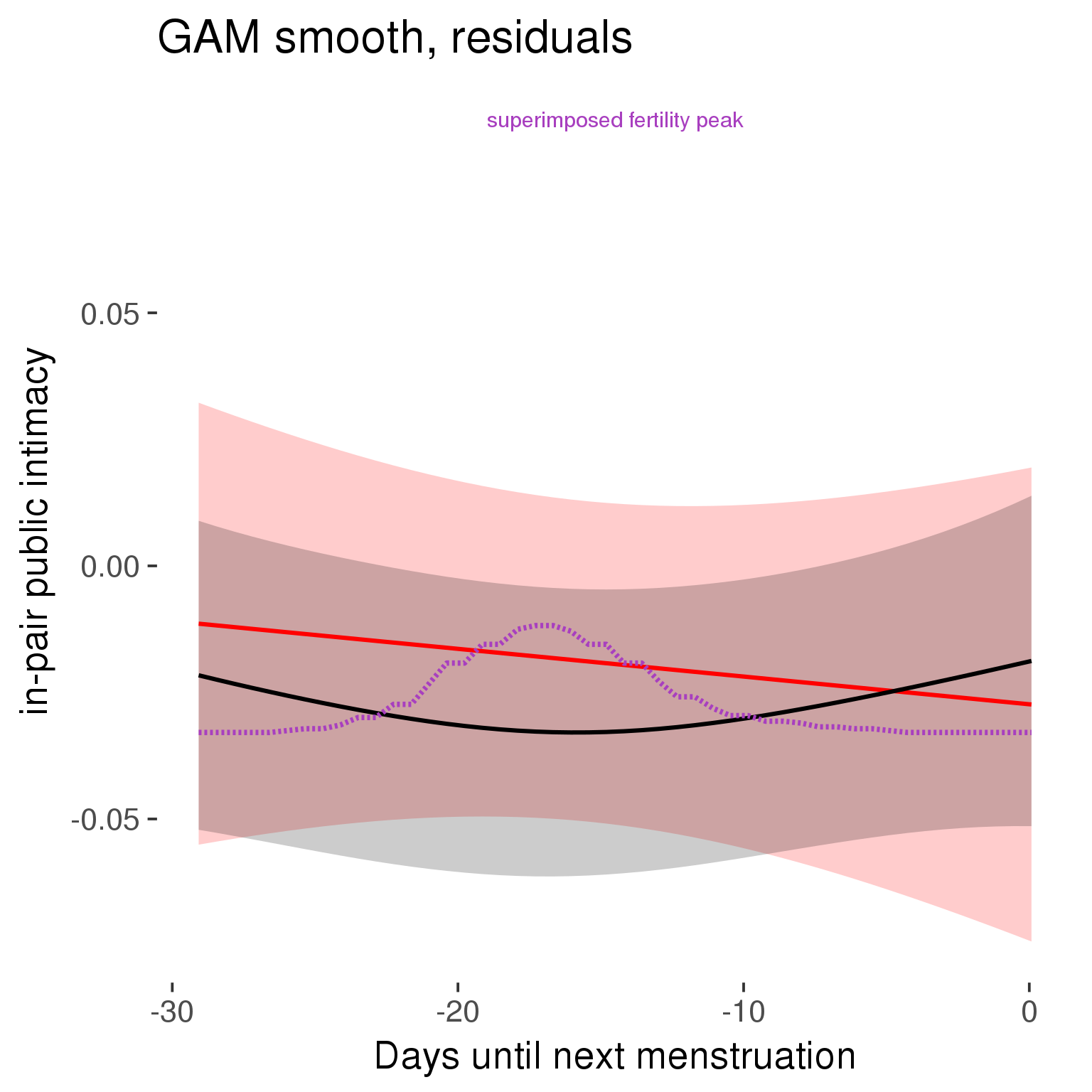
GAM smooth on raw data
As before, but without partialling anything out.
tryCatch({
trend_plot = ggplot(tmp,aes_string(x = "RCD", y = outcome, colour = "included")) +
stat_smooth(geom = 'smooth',size = 0.8, fill = "#9ECAE1", method = 'gam', formula = y ~ s(x))
}, error = function(e){cat_message(e, "danger")})
tryCatch({
trend_data = ggplot_build(trend_plot)$data[[1]]
}, error = function(e){cat_message(e, "danger")})
trend_data$RCD = round(trend_data$x)
trend_data = left_join(trend_data, tmp %>% select(real, RCD,fertile) %>% unique(), by = "RCD")
trend_data %>%
filter(real == TRUE) %>%
mutate(superimposed = ( ( (fertile - 0.01)/0.58) * (max(y)-min(y) ) ) + min(y) ) ->
trend_data
plot1b = ggplot(trend_data) +
geom_ribbon(aes(x = x, ymin = ymin, ymax = ymax, fill = factor(group)), alpha = 0.2) +
geom_line(aes(x = x, y = y, colour = factor(group)), size = 0.8, stat = "identity") +
scale_x_continuous(caption_x) +
geom_line(aes(x = x, y = superimposed), color = "#a83fbf", size = 1, linetype = 'dashed') +
annotate("text",x = mean(trend_data$x), y = max(trend_data$superimposed,na.rm=T) + 0.1, label = 'superimposed fertility peak', color = "#a83fbf") +
scale_y_continuous(outcome_label) +
ggtitle("GAM smooth, raw data") +
scale_color_manual("Contraception status",values = c("2"="black","1"= "red"), labels = c("2"="hormonally\ncontracepting","1"="cycling"), guide = F) +
scale_fill_manual("Contraception status",values = c("2"="black","1"= "red"), labels = c("2"="hormonally\ncontracepting","1"="cycling"), guide = F)
suppressWarnings(print(plot1b))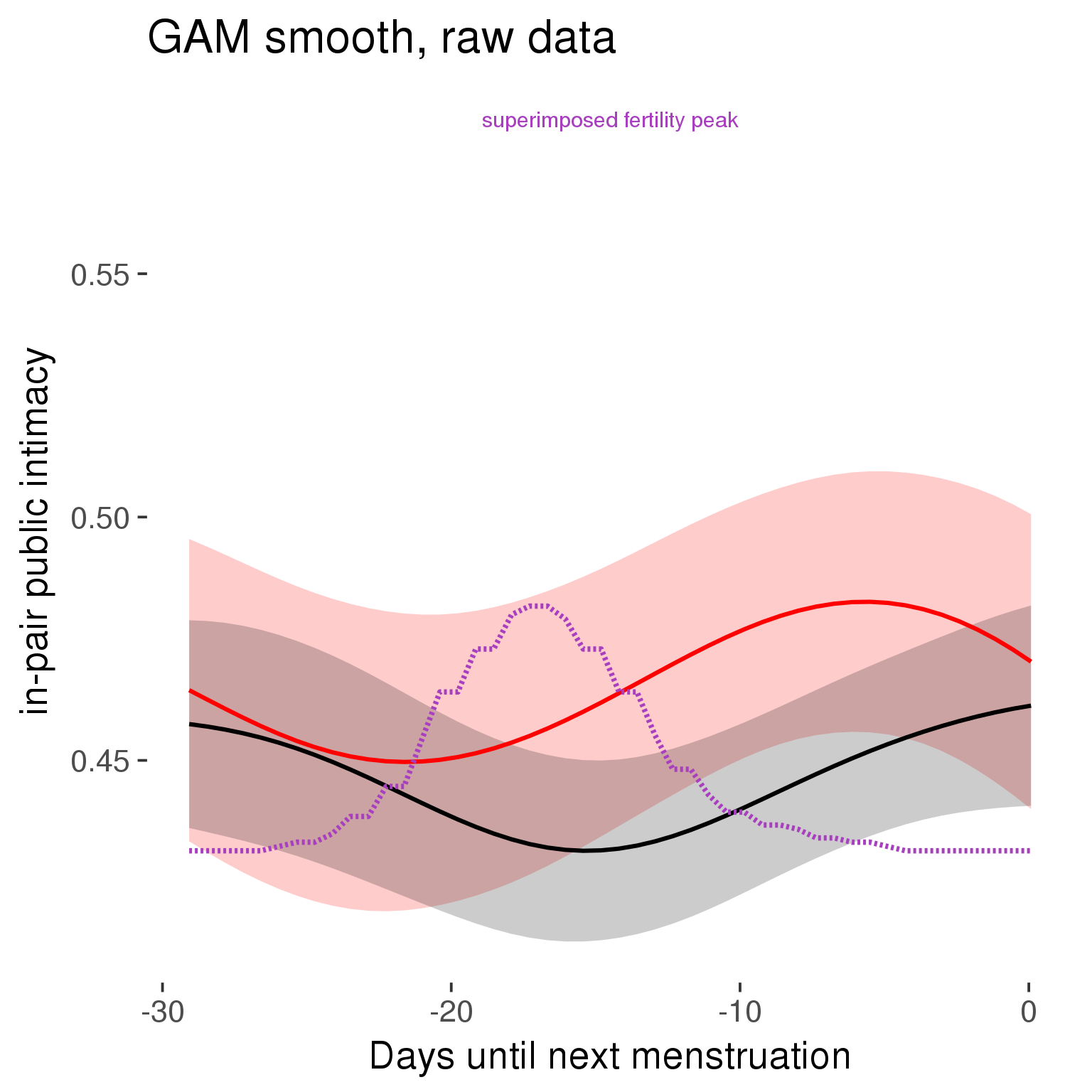
Means and standard errors over raw data
Nothing partialled out, just straight means with bootstrapped confidence intervals.
tryCatch({
trend_plot = ggplot(tmp,aes_string(x = "RCD", y = outcome, colour = "included")) +
geom_pointrange(size = 0.8, stat = 'summary', fun.data = "mean_cl_boot")
}, error = function(e){cat_message(e, "danger")})
tryCatch({
trend_data = ggplot_build(trend_plot)$data[[1]]
}, error = function(e){cat_message(e, "danger")})
trend_data$RCD = round(trend_data$x)
trend_data = left_join(trend_data, tmp %>% select(real, RCD,fertile) %>% unique(), by = "RCD")
trend_data %>%
filter(real == TRUE) %>%
mutate(superimposed = ( ( (fertile - 0.01)/0.58) * (max(y)-min(y) ) ) + min(y) ) ->
trend_data
plot3 = ggplot(trend_data) +
geom_pointrange(aes(x = x, y = y, ymin = ymin,ymax = ymax, colour = factor(group)), size = 0.8, stat = "identity", alpha = 0.6, position = position_dodge(width = .5)) +
scale_x_continuous("Days until next menstruation") +
geom_line(aes(x= x, y = superimposed), color = "#a83fbf", size = 1, linetype = 'dashed') +
annotate("text",x = mean(trend_data$x), y = max(trend_data$superimposed,na.rm=T) + 0.1, label = 'superimposed fertility peak', color = "#a83fbf") +
scale_y_continuous(outcome_label) +
ggtitle("Means with standard errors, raw data") +
scale_color_manual("Contraception status",values = c("2"="black","1"= "red"), labels = c("2"="hormonally\ncontracepting","1"="cycling"), guide = F) +
scale_fill_manual("Contraception status",values = c("2"="black","1"= "red"), labels = c("2"="hormonally\ncontracepting","1"="cycling"), guide = F)
suppressWarnings(print(plot3))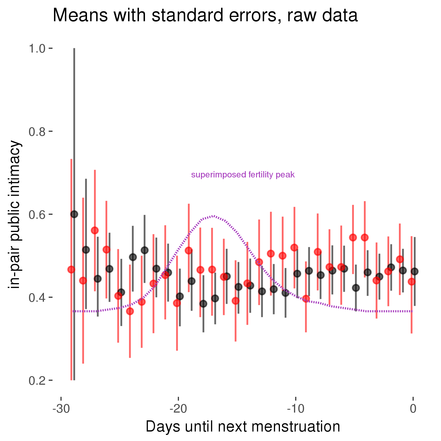
Forward-counted
model %>%
plot_curve(diary %>% filter(minimum_cycle_length_diary <= 30, minimum_cycle_length_diary >= 27) %>% mutate(RCD = FCD, fertile = prc_stirn_b_forward_counted), caption_x = "Days since last menstruation")outcome = names(model@frame)[1]
outcome_label = recode(str_replace_all(str_replace_all(str_replace_all(outcome, "_", " "), " pair", "-pair"), " 1", ""),
"desirability 1" = "self-perceived desirability",
"NARQ admiration" = "narcissistic admiration",
"NARQ rivalry" = "narcissistic rivalry",
"extra-pair" = "extra-pair desire & behaviour",
"had sexual intercourse" = "sexual intercourse")
library(ggplot2)
# form a subset and run the model without the hormonal contraception and the fertility predictors
tmp = diary %>%
filter(!is.na(fertile), !is.na(included),
RCD > -1 * minimum_cycle_length_diary, RCD > -40)
new_form = update.formula(formula(model), new = . ~ . - fertile * included)
tmp$residuals = residuals(update(model, new_form, data = tmp , na.action = na.exclude))
tmp = tmp %>%
filter(!is.na(RCD), !is.na(residuals))
rcd_min = min(tmp$RCD)
tmp$real = FALSE
tmp_before = tmp
tmp_before$RCD = tmp_before$RCD + min(tmp$RCD) - 1
tmp_after = tmp
tmp_after$RCD = tmp_after$RCD - min(tmp$RCD) + 1
tmp$real = TRUE
tmp = bind_rows(tmp_before %>% filter(RCD > rcd_min - 11), tmp, tmp_after %>% filter(RCD < 11))GAM smooth on residuals
Here, we partialled out menstruation and individual random effects, then superimposed estimated probability of being in the fertile window scaled to the range of the estimated means. To address the periodicity of the cycle, we prepended and appended ten days of the timeseries to the end and the beginning of the timeseries. We then estimated the GAM and cut off the appended subsets before plotting.
tryCatch({
trend_plot = ggplot(tmp,aes(x = RCD, y = residuals, colour = included)) +
stat_smooth(geom = 'smooth',size = 0.8, fill = "#9ECAE1", method = 'gam', formula = y ~ s(x))
}, error = function(e){cat_message(e, "danger")})
tryCatch({
trend_data = ggplot_build(trend_plot)$data[[1]]
}, error = function(e){cat_message(e, "danger")})
trend_data$RCD = round(trend_data$x)
trend_data = left_join(trend_data, tmp %>% select(real, RCD,fertile) %>% unique(), by = "RCD")
trend_data %>%
filter(real == TRUE) %>%
mutate(superimposed = ( ( (fertile - 0.01)/0.58) * (max(y)-min(y) ) ) + min(y) ) ->
trend_data
ggplot(trend_data) +
geom_ribbon(aes(x = x, ymin = ymin, ymax = ymax, fill = factor(group)), alpha = 0.2) +
geom_line(aes(x = x, y = y, colour = factor(group)), size = 0.8, stat = "identity") +
scale_x_continuous(caption_x) +
geom_line(aes(x = x, y = superimposed), color = "#a83fbf", size = 1, linetype = 'dashed') +
annotate("text",x = mean(trend_data$x), y = max(trend_data$superimposed,na.rm=T) + 0.1, label = 'superimposed fertility peak', color = "#a83fbf") +
scale_y_continuous(outcome_label) +
ggtitle("GAM smooth, residuals") +
scale_color_manual("Contraception status",values = c("2"="black","1"= "red"), labels = c("2"="hormonally\ncontracepting","1"="cycling"), guide = F) +
scale_fill_manual("Contraception status",values = c("2"="black","1"= "red"), labels = c("2"="hormonally\ncontracepting","1"="cycling"), guide = F)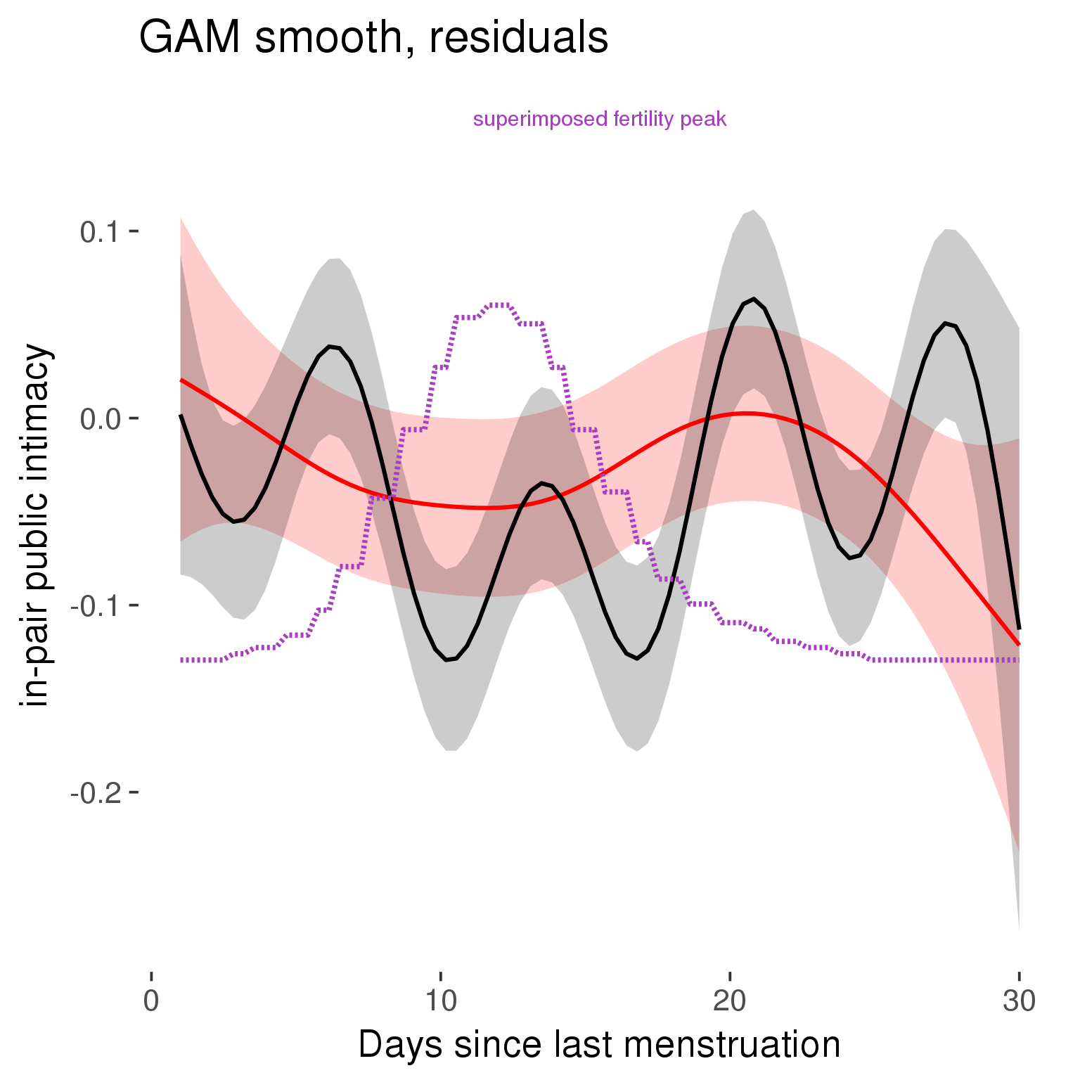
GAM smooth on raw data
As before, but without partialling anything out.
tryCatch({
trend_plot = ggplot(tmp,aes_string(x = "RCD", y = outcome, colour = "included")) +
stat_smooth(geom = 'smooth',size = 0.8, fill = "#9ECAE1", method = 'gam', formula = y ~ s(x))
}, error = function(e){cat_message(e, "danger")})
tryCatch({
trend_data = ggplot_build(trend_plot)$data[[1]]
}, error = function(e){cat_message(e, "danger")})
trend_data$RCD = round(trend_data$x)
trend_data = left_join(trend_data, tmp %>% select(real, RCD,fertile) %>% unique(), by = "RCD")
trend_data %>%
filter(real == TRUE) %>%
mutate(superimposed = ( ( (fertile - 0.01)/0.58) * (max(y)-min(y) ) ) + min(y) ) ->
trend_data
plot1b = ggplot(trend_data) +
geom_ribbon(aes(x = x, ymin = ymin, ymax = ymax, fill = factor(group)), alpha = 0.2) +
geom_line(aes(x = x, y = y, colour = factor(group)), size = 0.8, stat = "identity") +
scale_x_continuous(caption_x) +
geom_line(aes(x = x, y = superimposed), color = "#a83fbf", size = 1, linetype = 'dashed') +
annotate("text",x = mean(trend_data$x), y = max(trend_data$superimposed,na.rm=T) + 0.1, label = 'superimposed fertility peak', color = "#a83fbf") +
scale_y_continuous(outcome_label) +
ggtitle("GAM smooth, raw data") +
scale_color_manual("Contraception status",values = c("2"="black","1"= "red"), labels = c("2"="hormonally\ncontracepting","1"="cycling"), guide = F) +
scale_fill_manual("Contraception status",values = c("2"="black","1"= "red"), labels = c("2"="hormonally\ncontracepting","1"="cycling"), guide = F)
suppressWarnings(print(plot1b))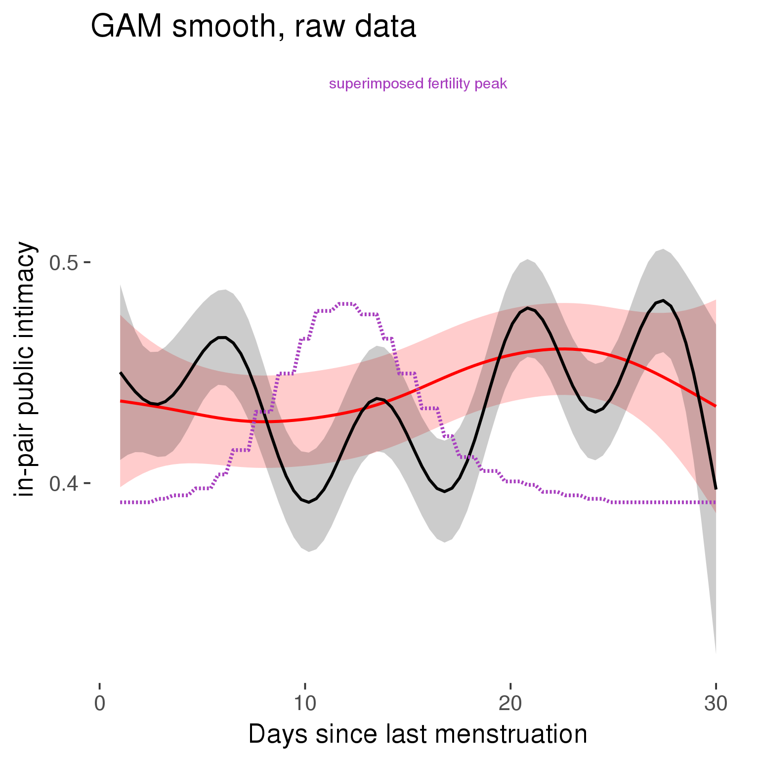
Means and standard errors over raw data
Nothing partialled out, just straight means with bootstrapped confidence intervals.
tryCatch({
trend_plot = ggplot(tmp,aes_string(x = "RCD", y = outcome, colour = "included")) +
geom_pointrange(size = 0.8, stat = 'summary', fun.data = "mean_cl_boot")
}, error = function(e){cat_message(e, "danger")})
tryCatch({
trend_data = ggplot_build(trend_plot)$data[[1]]
}, error = function(e){cat_message(e, "danger")})
trend_data$RCD = round(trend_data$x)
trend_data = left_join(trend_data, tmp %>% select(real, RCD,fertile) %>% unique(), by = "RCD")
trend_data %>%
filter(real == TRUE) %>%
mutate(superimposed = ( ( (fertile - 0.01)/0.58) * (max(y)-min(y) ) ) + min(y) ) ->
trend_data
plot3 = ggplot(trend_data) +
geom_pointrange(aes(x = x, y = y, ymin = ymin,ymax = ymax, colour = factor(group)), size = 0.8, stat = "identity", alpha = 0.6, position = position_dodge(width = .5)) +
scale_x_continuous("Days until next menstruation") +
geom_line(aes(x= x, y = superimposed), color = "#a83fbf", size = 1, linetype = 'dashed') +
annotate("text",x = mean(trend_data$x), y = max(trend_data$superimposed,na.rm=T) + 0.1, label = 'superimposed fertility peak', color = "#a83fbf") +
scale_y_continuous(outcome_label) +
ggtitle("Means with standard errors, raw data") +
scale_color_manual("Contraception status",values = c("2"="black","1"= "red"), labels = c("2"="hormonally\ncontracepting","1"="cycling"), guide = F) +
scale_fill_manual("Contraception status",values = c("2"="black","1"= "red"), labels = c("2"="hormonally\ncontracepting","1"="cycling"), guide = F)
suppressWarnings(print(plot3))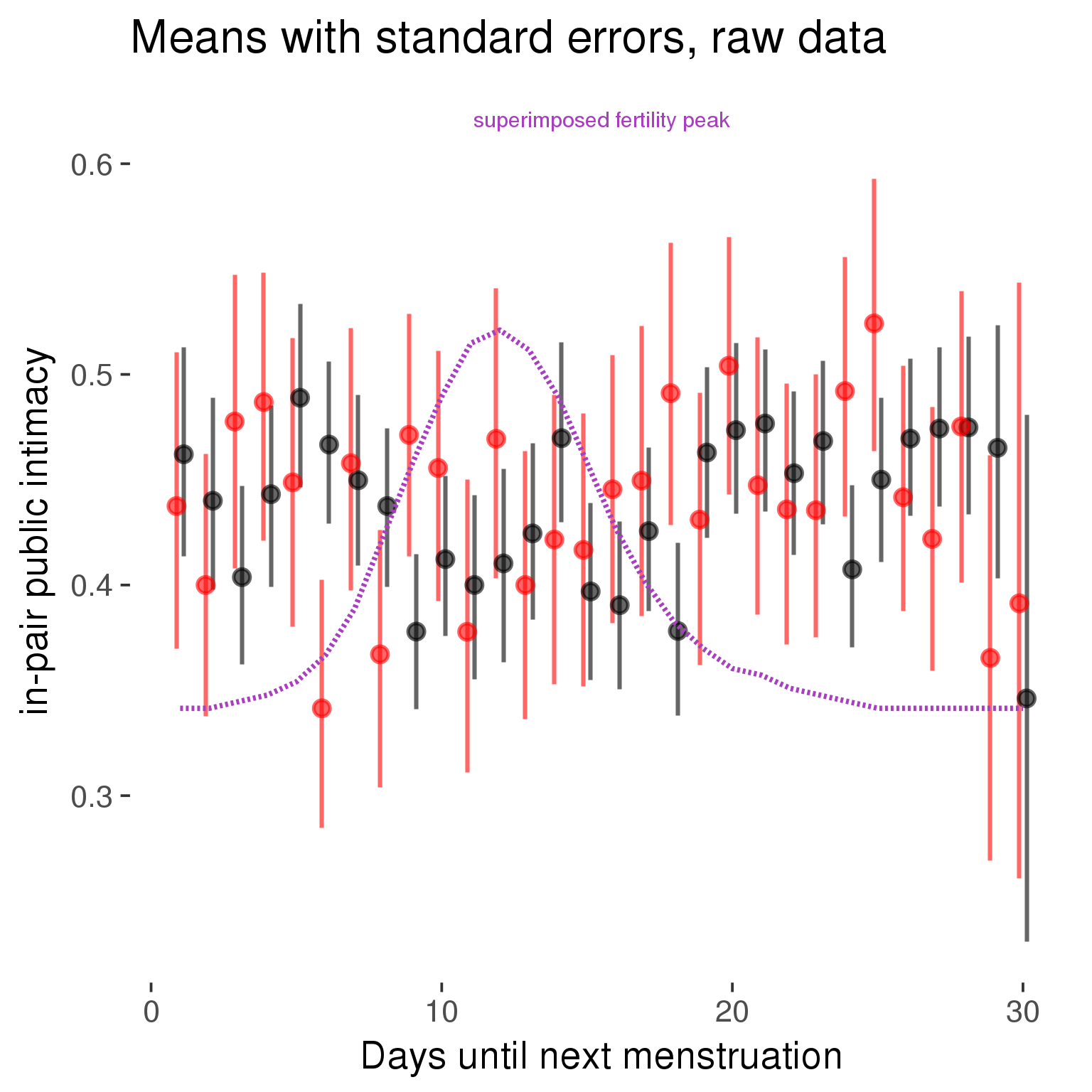
Robustness checks
M_r1: Random slopes for conception risk and menstruation
tryCatch({
# refit model with random effects for fertile and menstruation dummies
with_ind_diff = update(model, formula = . ~ . - (1| person) + (1 + fertile + menstruation | person))
# pull the random effects, format as tibble
rand = coef(with_ind_diff)$person %>%
tibble::rownames_to_column("person") %>%
mutate(person = as.numeric(person))
# pull the fixed effects
fixd = data.frame(fixef(with_ind_diff)) %>%
tibble::rownames_to_column("effect")
names(fixd) = c("effect", "pop_effect_size")
# pull apart the coefficients so that we can account for the fact that the random effect variation implicitly includes HC explaining the mean population-level effect of fertile/menstruation dummies among HC users
fixd = fixd %>%
separate(effect, c("included", "effect"), sep = ":", fill = "left") %>%
mutate(included = if_else(is.na(included), "cycling", str_replace(included, "included", "")))
fixd[2,c("included", "effect")] = c("horm_contra", "(Intercept)")
rand = rand %>%
# merge diary data on the random effects, so that we know who is a HC users and who isn't
inner_join(diary %>% select(person, included) %>% unique(), by = 'person') %>%
# gather into long format, to have the dataset by predictor
gather(effect, value, -person, -included) %>%
inner_join(fixd, by = c('effect', 'included')) %>%
# pull the fixed effects
mutate(
# only for those who are HC users, add the moderated population effect size for this effect (the random effects have the reference category mean)
value = if_else(included == "horm_contra", value + pop_effect_size, value),
effect = recode(effect, "includedhorm_contra" = "HC user",
"includedhorm_contra:fertile" = "HC user x fertile",
"includedhorm_contra:menstruationpre" = "HC user x premens.",
"includedhorm_contra:menstruationyes" = "HC user x mens.",
"menstruationyes" = "mens.",
"menstruationpre" = "premens.")) %>%
group_by(included, effect) %>%
# filter out predictors that aren't modelled as varying/random
filter(sd(value) > 0)
# plot dot plot of random effects
print(
ggplot(rand, aes(x = included, y = value, color = included, fill = included)) +
facet_wrap( ~ effect, scales = "free") +
# geom_violin(alpha = 0.4, size = 0) +
geom_dotplot(binaxis='y', dotsize = 0.1, method = "histodot") +
# geom_jitter(alpha = 0.05) +
coord_flip() +
geom_pointrange(stat = 'summary', fun.data = 'mean_sdl', color = 'darkred', size = 1.2) +
scale_color_manual("Contraception status", values = c("horm_contra"="black","cycling"= "red"), labels = c("horm_contra"="hormonally\ncontracepting","cycling"="cycling"), guide = F) +
scale_fill_manual("Contraception status", values = c("horm_contra"="black","cycling"= "red"), labels = c("horm_contra"="hormonally\ncontracepting","1"="cycling"), guide = F) +
ggtitle("M_r1: allowing participant-varying slopes", subtitle = "for the conception risk measure and the menstruation dummies") +
scale_x_discrete("Hormonal contraception", breaks = c("horm_contra", "cycling"), labels = c("yes", "no")) +
scale_y_continuous("Random effect size distribution"))
print_summary(with_ind_diff)
cat(pander(anova(model, with_ind_diff)))
}, error = function(e){
with_ind_diff = model
cat_message(e, "danger")
})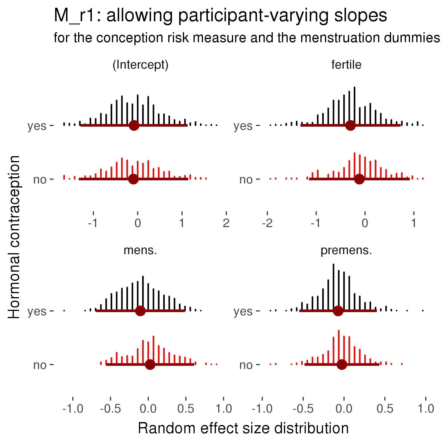
Generalized linear mixed model fit by maximum likelihood (Laplace Approximation) ['glmerMod']
Family: binomial ( probit )
Formula: in_pair_public_intimacy ~ included + menstruation + fertile +
fertile_mean + (1 + fertile + menstruation | person) + included:menstruation + included:fertile
Data: diary
AIC BIC logLik deviance df.resid
32792 32948 -16377 32754 26685
Scaled residuals:
Min 1Q Median 3Q Max
-3.766 -0.739 -0.314 0.812 3.554
Random effects:
Groups Name Variance Std.Dev. Corr
person (Intercept) 0.551 0.742
fertile 1.047 1.023 -0.28
menstruationpre 0.230 0.479 -0.32 0.21
menstruationyes 0.287 0.535 0.17 0.18 0.42
Number of obs: 26704, groups: person, 1054
Fixed effects:
Estimate Std. Error z value Pr(>|z|)
(Intercept) -0.0996 0.0736 -1.35 0.176
includedhorm_contra 0.0134 0.0606 0.22 0.825
menstruationpre -0.0258 0.0508 -0.51 0.612
menstruationyes 0.0248 0.0518 0.48 0.633
fertile -0.1180 0.1052 -1.12 0.262
fertile_mean 0.1869 0.3423 0.55 0.585
includedhorm_contra:menstruationpre -0.0471 0.0651 -0.72 0.469
includedhorm_contra:menstruationyes -0.1323 0.0677 -1.96 0.051 .
includedhorm_contra:fertile -0.1831 0.1329 -1.38 0.168
---
Signif. codes: 0 '***' 0.001 '**' 0.01 '*' 0.05 '.' 0.1 ' ' 1
Correlation of Fixed Effects:
(Intr) incld_ mnstrtnp mnstrtny fertil frtl_m inclddhrm_cntr:mnstrtnp
inclddhrm_c -0.477
menstrutnpr -0.290 0.342
menstrutnys -0.124 0.161 0.390
fertile -0.245 0.391 0.383 0.305
fertile_men -0.766 -0.033 0.011 -0.011 -0.098
inclddhrm_cntr:mnstrtnp 0.231 -0.430 -0.780 -0.304 -0.298 -0.014
inclddhrm_cntr:mnstrtny 0.103 -0.193 -0.299 -0.766 -0.232 -0.002 0.380
inclddhrm_cntr:f 0.243 -0.496 -0.304 -0.240 -0.784 0.013 0.383
inclddhrm_cntr:mnstrtny
inclddhrm_c
menstrutnpr
menstrutnys
fertile
fertile_men
inclddhrm_cntr:mnstrtnp
inclddhrm_cntr:mnstrtny
inclddhrm_cntr:f 0.302
convergence code: 0
Model failed to converge with max|grad| = 0.0191849 (tol = 0.001, component 1)
| Df | AIC | BIC | logLik | deviance | Chisq | Chi Df | Pr(>Chisq) | |
|---|---|---|---|---|---|---|---|---|
| model | 10 | 33038 | 33120 | -16509 | 33018 | NA | NA | NA |
| with_ind_diff | 19 | 32792 | 32948 | -16377 | 32754 | 263.8 | 9 | 1.235e-51 |
robustness_check_ovu_shift(model, diary)M_e: Exclusion criteria
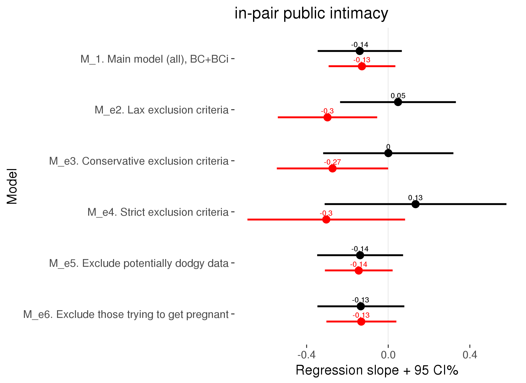
M_p: Predictors
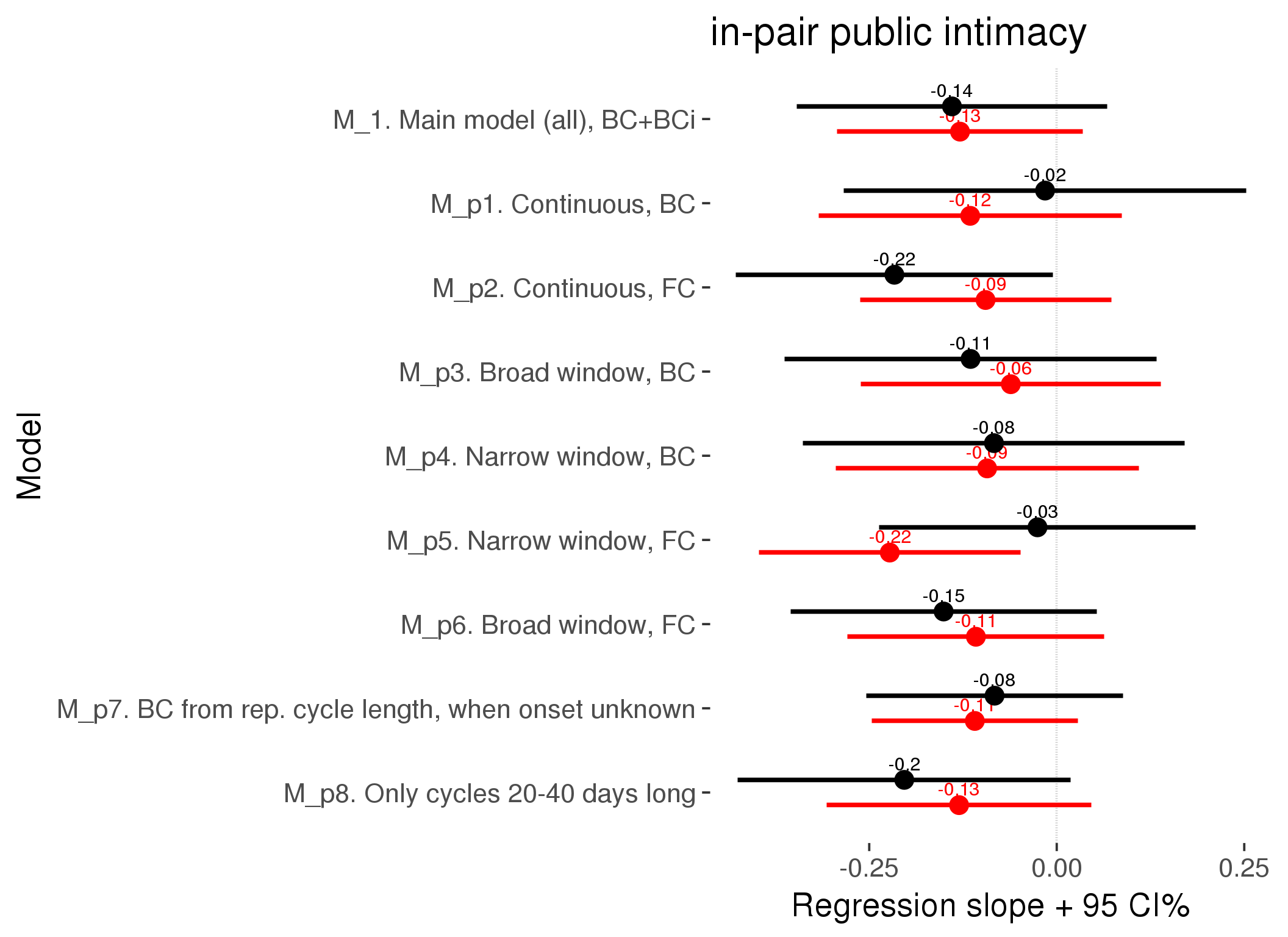
M_c: Covariates, controls, autocorrelation
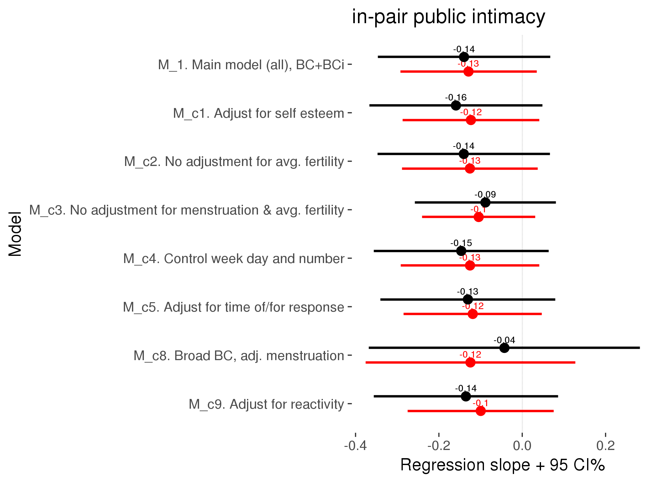
Generalized linear mixed model fit by maximum likelihood (Laplace Approximation) ['glmerMod']
Family: binomial ( probit )
AIC BIC logLik deviance df.resid
30047 30192 -15005 30011 24380
Scaled residuals:
Min 1Q Median 3Q Max
-3.693 -0.766 -0.326 0.855 3.866
Random effects:
Groups Name Variance Std.Dev.
person (Intercept) 0.508 0.713
Xr.2 s(days_filled_out):includedhorm_contra 0.253 0.503
Xr.1 s(days_filled_out):includedcycling 0.141 0.376
Xr.0 s(day_number):includedhorm_contra 0.193 0.439
Xr s(day_number):includedcycling 0.199 0.446
Number of obs: 24398, groups: person, 1054; Xr.2, 8; Xr.1, 8; Xr.0, 8; Xr, 8
Fixed effects:
Estimate Std. Error z value Pr(>|z|)
X(Intercept) -0.129365 0.072562 -1.78 0.0746 .
Xincludedhorm_contra 0.000986 0.060018 0.02 0.9869
Xmenstruationpre 0.002863 0.043301 0.07 0.9473
Xmenstruationyes 0.026246 0.041796 0.63 0.5300
Xfertile -0.099577 0.089386 -1.11 0.2653
Xfertile_mean 0.162113 0.334123 0.49 0.6275
Xincludedhorm_contra:menstruationpre -0.034046 0.055428 -0.61 0.5391
Xincludedhorm_contra:menstruationyes -0.100635 0.054642 -1.84 0.0655 .
Xincludedhorm_contra:fertile -0.135200 0.112844 -1.20 0.2309
Xs(day_number):includedcyclingFx1 0.472751 0.218935 2.16 0.0308 *
Xs(day_number):includedhorm_contraFx1 0.542261 0.170617 3.18 0.0015 **
Xs(days_filled_out):includedcyclingFx1 -0.218097 0.157483 -1.38 0.1661
Xs(days_filled_out):includedhorm_contraFx1 -0.498022 0.170528 -2.92 0.0035 **
---
Signif. codes: 0 '***' 0.001 '**' 0.01 '*' 0.05 '.' 0.1 ' ' 1
Family: binomial
Link function: probit
Formula:
in_pair_public_intimacy ~ included + menstruation + fertile +
fertile_mean + s(day_number, by = included) + s(days_filled_out,
by = included) + included:menstruation + included:fertile
Parametric coefficients:
Estimate Std. Error z value Pr(>|z|)
(Intercept) -0.129365 0.071098 -1.82 0.069 .
includedhorm_contra 0.000986 0.059335 0.02 0.987
menstruationpre 0.002863 0.042758 0.07 0.947
menstruationyes 0.026246 0.041019 0.64 0.522
fertile -0.099577 0.088052 -1.13 0.258
fertile_mean 0.162113 0.325606 0.50 0.619
includedhorm_contra:menstruationpre -0.034046 0.054734 -0.62 0.534
includedhorm_contra:menstruationyes -0.100635 0.053632 -1.88 0.061 .
includedhorm_contra:fertile -0.135200 0.111221 -1.22 0.224
---
Signif. codes: 0 '***' 0.001 '**' 0.01 '*' 0.05 '.' 0.1 ' ' 1
Approximate significance of smooth terms:
edf Ref.df Chi.sq p-value
s(day_number):includedcycling 3.78 3.78 18.9 0.00084 ***
s(day_number):includedhorm_contra 4.00 4.00 56.5 0.000000000016 ***
s(days_filled_out):includedcycling 3.32 3.32 16.7 0.00154 **
s(days_filled_out):includedhorm_contra 4.42 4.42 58.1 0.000000000019 ***
---
Signif. codes: 0 '***' 0.001 '**' 0.01 '*' 0.05 '.' 0.1 ' ' 1
R-sq.(adj) = 0.00368
glmer.ML = 27242 Scale est. = 1 n = 24398

M_d: Other designs
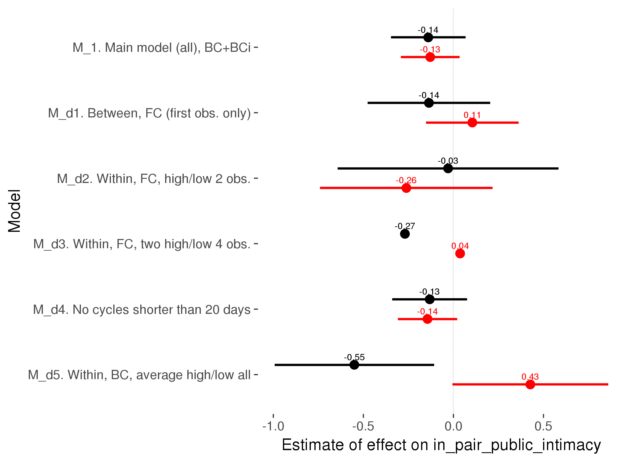
M_m1: Moderation by contraceptive method
Based on the sample with lax exclusion criteria. Users who used any hormonal contraception are classified as hormonal, users who use any awareness-based methods (counting, temperature-based) are classified as ‘fertility-awareness’, women who don’t fall into the before groups and use condoms, pessars, coitus interruptus etc. are classified as ‘barrie or abstinence’. Women who don’t use contraception or use other methods such as sterilisation are excluded from this analysis.
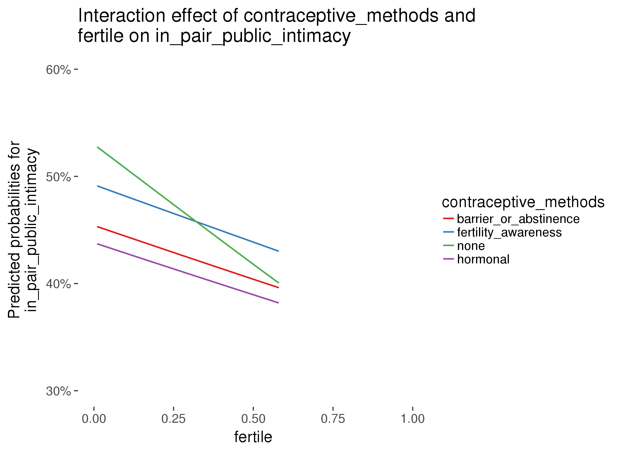
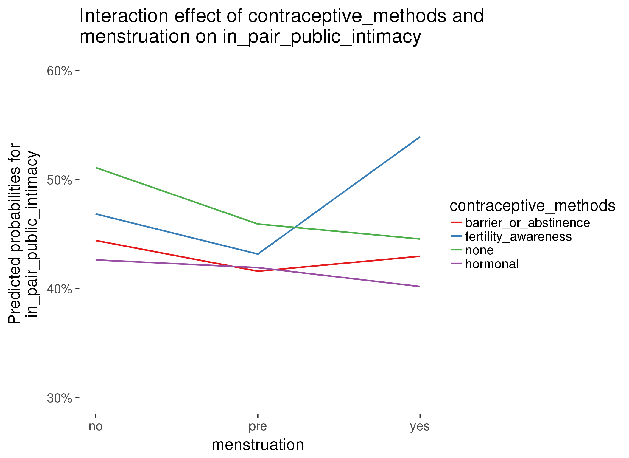
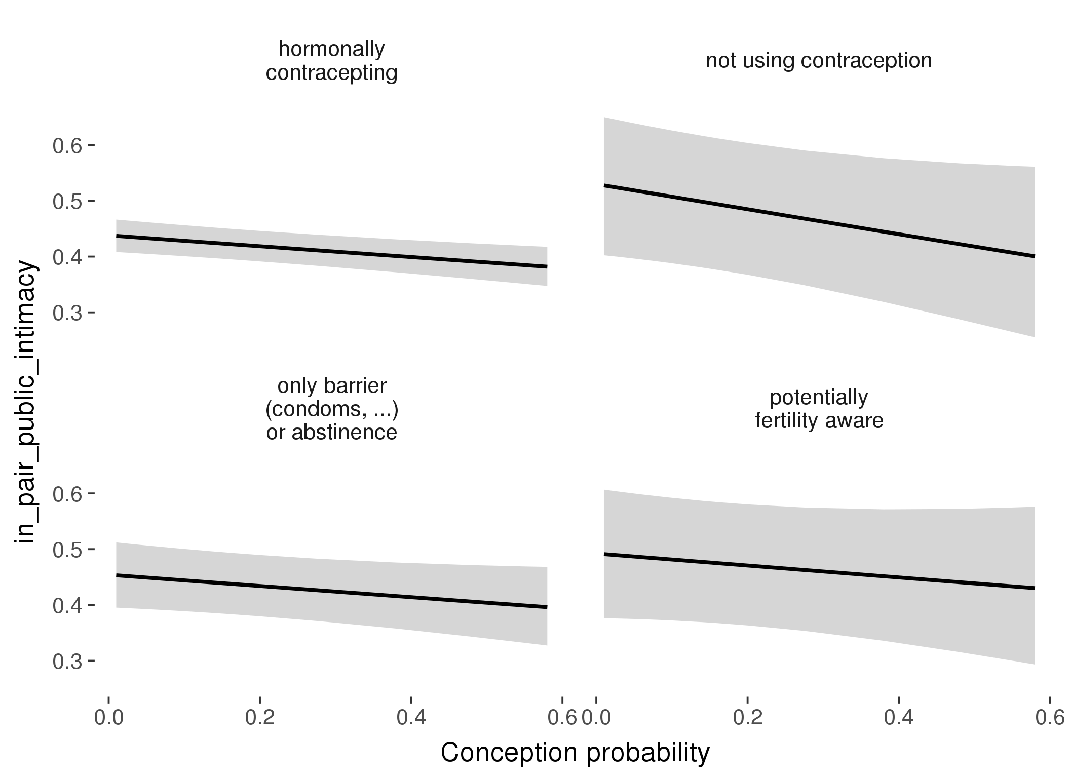
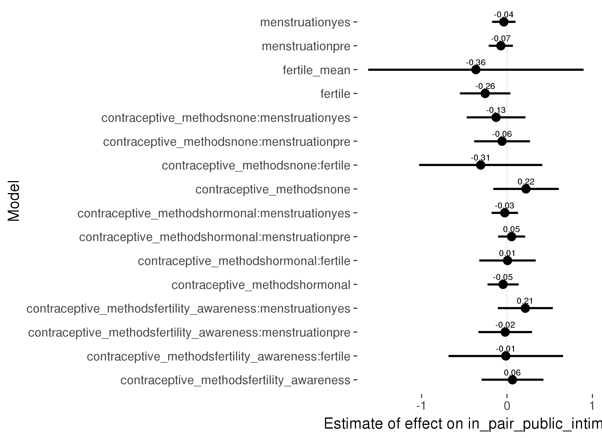
Generalized linear mixed model fit by maximum likelihood (Laplace Approximation) ['glmerMod']
Family: binomial ( probit )
Formula: in_pair_public_intimacy ~ fertile_mean + (1 | person) + contraceptive_methods +
fertile + menstruation + fertile:contraceptive_methods + menstruation:contraceptive_methods
Data: diary
Subset: !is.na(included_lax) & contraceptive_method != "other"
AIC BIC logLik deviance df.resid
21215 21355 -10590 21179 17026
Scaled residuals:
Min 1Q Median 3Q Max
-3.141 -0.777 -0.436 0.902 3.555
Random effects:
Groups Name Variance Std.Dev.
person (Intercept) 0.414 0.643
Number of obs: 17044, groups: person, 513
Fixed effects:
Estimate Std. Error z value Pr(>|z|)
(Intercept) -0.03174 0.13430 -0.24 0.813
fertile_mean -0.36448 0.64368 -0.57 0.571
contraceptive_methodsfertility_awareness 0.06382 0.18492 0.34 0.730
contraceptive_methodsnone 0.22205 0.19564 1.14 0.256
contraceptive_methodshormonal -0.04637 0.09254 -0.50 0.616
fertile -0.25582 0.15062 -1.70 0.089 .
menstruationpre -0.07181 0.07232 -0.99 0.321
menstruationyes -0.03669 0.06947 -0.53 0.597
contraceptive_methodsfertility_awareness:fertile -0.01385 0.34180 -0.04 0.968
contraceptive_methodsnone:fertile -0.30801 0.36731 -0.84 0.402
contraceptive_methodshormonal:fertile 0.00643 0.16802 0.04 0.969
contraceptive_methodsfertility_awareness:menstruationpre -0.02125 0.16056 -0.13 0.895
contraceptive_methodsnone:menstruationpre -0.05815 0.16714 -0.35 0.728
contraceptive_methodshormonal:menstruationpre 0.05366 0.08136 0.66 0.510
contraceptive_methodsfertility_awareness:menstruationyes 0.21421 0.16432 1.30 0.192
contraceptive_methodsnone:menstruationyes -0.12795 0.17593 -0.73 0.467
contraceptive_methodshormonal:menstruationyes -0.02604 0.07917 -0.33 0.742
---
Signif. codes: 0 '***' 0.001 '**' 0.01 '*' 0.05 '.' 0.1 ' ' 1
convergence code: 0
Model failed to converge with max|grad| = 0.00249015 (tol = 0.001, component 1)
| Df | AIC | BIC | logLik | deviance | Chisq | Chi Df | Pr(>Chisq) | |
|---|---|---|---|---|---|---|---|---|
| add_main | 12 | 21207 | 21300 | -10592 | 21183 | NA | NA | NA |
| by_method | 18 | 21215 | 21355 | -10590 | 21179 | 3.669 | 6 | 0.7213 |
M_m2: Moderation by participant age
model %>%
test_moderator("age_group", diary, xlevels = 5)| Df | AIC | BIC | logLik | deviance | Chisq | Chi Df | Pr(>Chisq) | |
|---|---|---|---|---|---|---|---|---|
| with_main | 18 | 33036 | 33183 | -16500 | 33000 | NA | NA | NA |
| with_mod | 26 | 33045 | 33258 | -16496 | 32993 | 6.636 | 8 | 0.5763 |
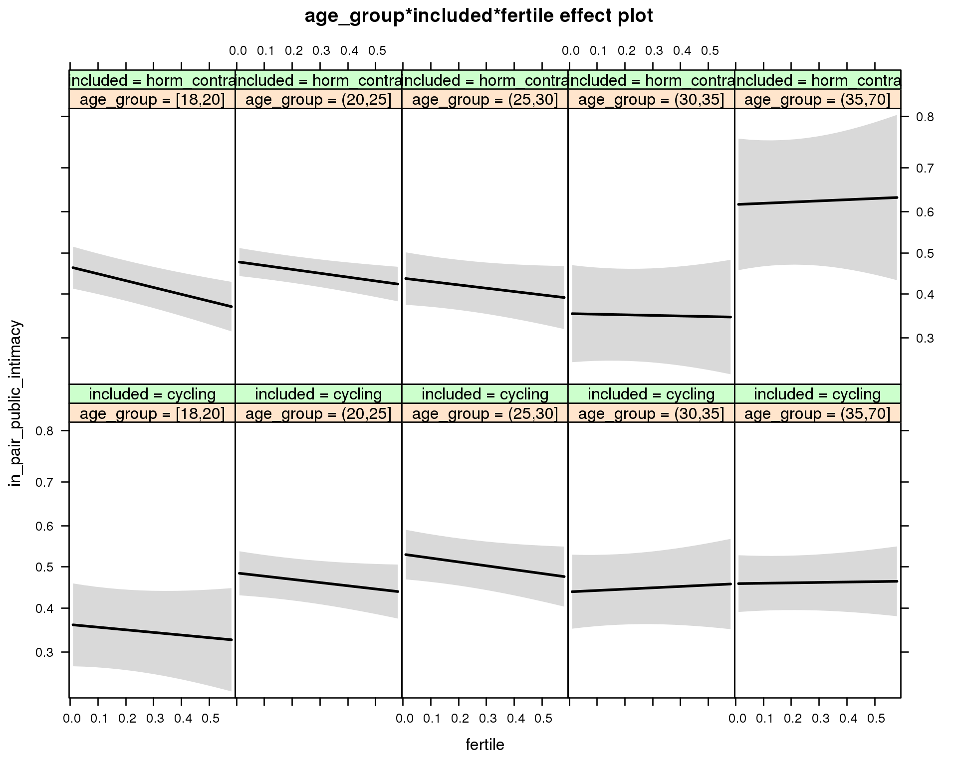
Generalized linear mixed model fit by maximum likelihood (Laplace Approximation) ['glmerMod']
Family: binomial ( probit )
Formula: in_pair_public_intimacy ~ menstruation + fertile_mean + (1 |
person) + age_group + included + fertile + menstruation:included +
age_group:included + age_group:fertile + included:fertile + age_group:included:fertile
Data: diary
AIC BIC logLik deviance df.resid
33045 33258 -16496 32993 26678
Scaled residuals:
Min 1Q Median 3Q Max
-4.033 -0.780 -0.352 0.857 4.130
Random effects:
Groups Name Variance Std.Dev.
person (Intercept) 0.474 0.688
Number of obs: 26704, groups: person, 1054
Fixed effects:
Estimate Std. Error z value Pr(>|z|)
(Intercept) -0.3740 0.1404 -2.66 0.0077 **
menstruationpre -0.0336 0.0413 -0.81 0.4158
menstruationyes 0.0279 0.0391 0.71 0.4750
fertile_mean 0.1118 0.3259 0.34 0.7315
age_group(20,25] 0.3185 0.1479 2.15 0.0313 *
age_group(25,30] 0.4340 0.1521 2.85 0.0043 **
age_group(30,35] 0.2021 0.1751 1.15 0.2485
age_group(35,70] 0.2526 0.1582 1.60 0.1103
includedhorm_contra 0.2916 0.1487 1.96 0.0499 *
fertile -0.1614 0.2386 -0.68 0.4986
menstruationpre:includedhorm_contra -0.0265 0.0528 -0.50 0.6156
menstruationyes:includedhorm_contra -0.1038 0.0511 -2.03 0.0423 *
age_group(20,25]:includedhorm_contra -0.2857 0.1680 -1.70 0.0889 .
age_group(25,30]:includedhorm_contra -0.5033 0.1854 -2.71 0.0066 **
age_group(30,35]:includedhorm_contra -0.4896 0.2419 -2.02 0.0430 *
age_group(35,70]:includedhorm_contra 0.1329 0.2698 0.49 0.6223
age_group(20,25]:fertile -0.0363 0.2650 -0.14 0.8910
age_group(25,30]:fertile -0.0765 0.2715 -0.28 0.7783
age_group(30,35]:fertile 0.2447 0.3165 0.77 0.4394
age_group(35,70]:fertile 0.1863 0.2843 0.66 0.5122
includedhorm_contra:fertile -0.2598 0.2638 -0.98 0.3248
age_group(20,25]:includedhorm_contra:fertile 0.2197 0.2959 0.74 0.4577
age_group(25,30]:includedhorm_contra:fertile 0.2925 0.3264 0.90 0.3702
age_group(30,35]:includedhorm_contra:fertile 0.1403 0.4296 0.33 0.7440
age_group(35,70]:includedhorm_contra:fertile 0.3092 0.5132 0.60 0.5469
---
Signif. codes: 0 '***' 0.001 '**' 0.01 '*' 0.05 '.' 0.1 ' ' 1
convergence code: 0
Model failed to converge with max|grad| = 0.0346393 (tol = 0.001, component 1)
M_m3: Moderation by weekend
model %>%
test_moderator("weekend", diary, xlevels = 2) | Df | AIC | BIC | logLik | deviance | Chisq | Chi Df | Pr(>Chisq) | |
|---|---|---|---|---|---|---|---|---|
| with_main | 12 | 32326 | 32424 | -16151 | 32302 | NA | NA | NA |
| with_mod | 14 | 32330 | 32444 | -16151 | 32302 | 0.553 | 2 | 0.7584 |
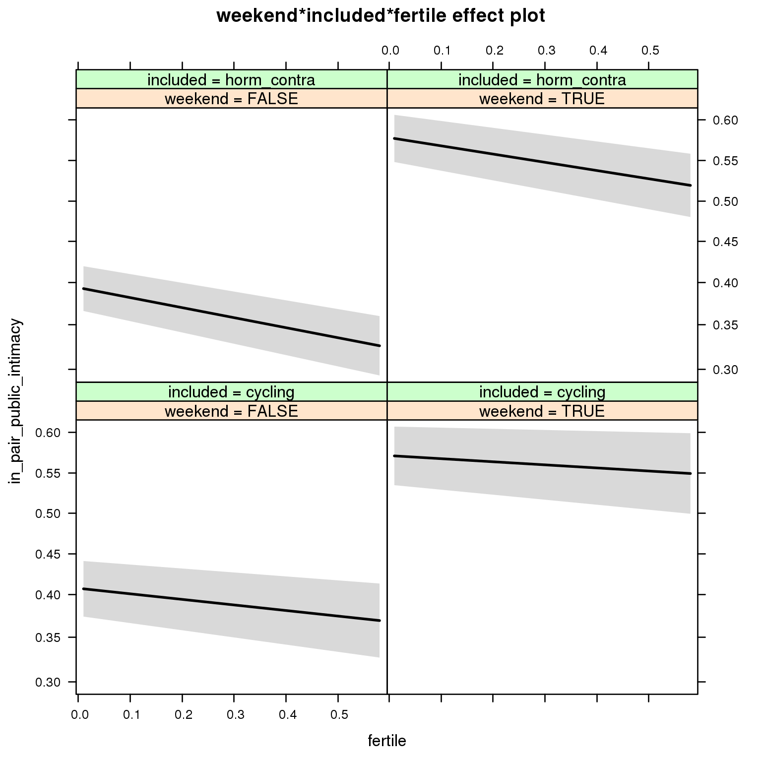
Generalized linear mixed model fit by maximum likelihood (Laplace Approximation) ['glmerMod']
Family: binomial ( probit )
Formula: in_pair_public_intimacy ~ menstruation + fertile_mean + (1 |
person) + weekend + included + fertile + menstruation:included +
weekend:included + weekend:fertile + included:fertile + weekend:included:fertile
Data: diary
AIC BIC logLik deviance df.resid
32330 32444 -16151 32302 26690
Scaled residuals:
Min 1Q Median 3Q Max
-4.709 -0.749 -0.327 0.815 4.336
Random effects:
Groups Name Variance Std.Dev.
person (Intercept) 0.51 0.714
Number of obs: 26704, groups: person, 1054
Fixed effects:
Estimate Std. Error z value Pr(>|z|)
(Intercept) -0.2611 0.0733 -3.56 0.00037 ***
menstruationpre -0.0354 0.0416 -0.85 0.39432
menstruationyes 0.0262 0.0394 0.66 0.50605
fertile_mean 0.1716 0.3340 0.51 0.60741
weekendTRUE 0.4132 0.0365 11.32 < 2e-16 ***
includedhorm_contra -0.0138 0.0615 -0.22 0.82213
fertile -0.1734 0.1033 -1.68 0.09305 .
menstruationpre:includedhorm_contra -0.0315 0.0533 -0.59 0.55486
menstruationyes:includedhorm_contra -0.0978 0.0516 -1.90 0.05805 .
weekendTRUE:includedhorm_contra 0.0539 0.0469 1.15 0.24982
weekendTRUE:fertile 0.0773 0.1413 0.55 0.58444
includedhorm_contra:fertile -0.1389 0.1313 -1.06 0.29003
weekendTRUE:includedhorm_contra:fertile -0.0214 0.1794 -0.12 0.90482
---
Signif. codes: 0 '***' 0.001 '**' 0.01 '*' 0.05 '.' 0.1 ' ' 1
M_m4: Moderation by weekday
model %>%
test_moderator("weekday", diary, xlevels = 7)| Df | AIC | BIC | logLik | deviance | Chisq | Chi Df | Pr(>Chisq) | |
|---|---|---|---|---|---|---|---|---|
| with_main | 22 | 32045 | 32226 | -16001 | 32001 | NA | NA | NA |
| with_mod | 34 | 32066 | 32344 | -15999 | 31998 | 3.726 | 12 | 0.9879 |
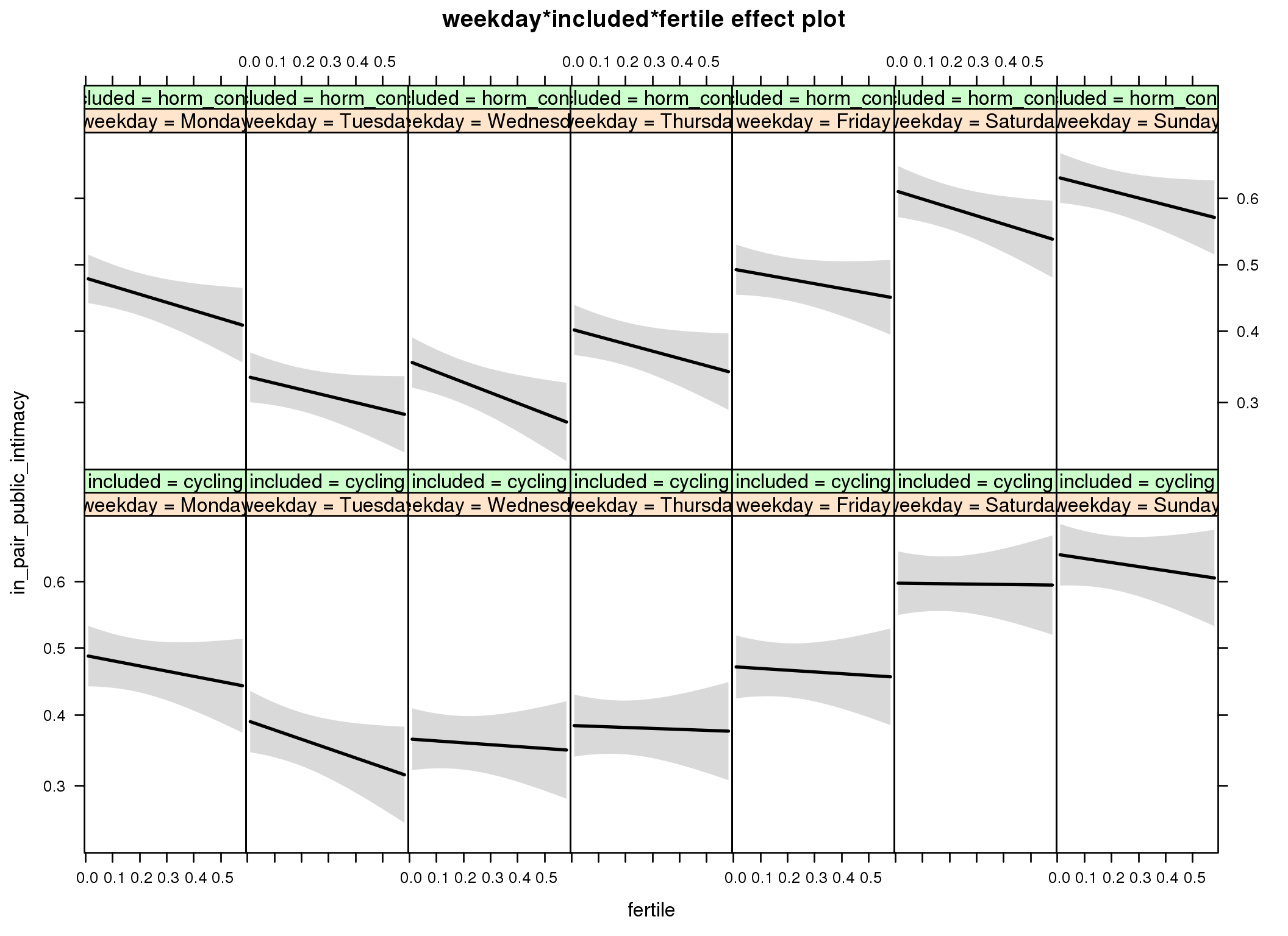
Generalized linear mixed model fit by maximum likelihood (Laplace Approximation) ['glmerMod']
Family: binomial ( probit )
Formula: in_pair_public_intimacy ~ menstruation + fertile_mean + (1 |
person) + weekday + included + fertile + menstruation:included +
weekday:included + weekday:fertile + included:fertile + weekday:included:fertile
Data: diary
AIC BIC logLik deviance df.resid
32066 32344 -15999 31998 26670
Scaled residuals:
Min 1Q Median 3Q Max
-5.524 -0.735 -0.317 0.806 4.096
Random effects:
Groups Name Variance Std.Dev.
person (Intercept) 0.522 0.722
Number of obs: 26704, groups: person, 1054
Fixed effects:
Estimate Std. Error z value Pr(>|z|)
(Intercept) -0.051260 0.083875 -0.61 0.54110
menstruationpre -0.033712 0.041828 -0.81 0.42025
menstruationyes 0.027459 0.039576 0.69 0.48779
fertile_mean 0.143785 0.337232 0.43 0.66984
weekdayTuesday -0.248217 0.065440 -3.79 0.00015 ***
weekdayWednesday -0.318063 0.065840 -4.83 0.0000013596 ***
weekdayThursday -0.266627 0.066269 -4.02 0.0000573605 ***
weekdayFriday -0.042717 0.066844 -0.64 0.52279
weekdaySaturday 0.275768 0.067653 4.08 0.0000457729 ***
weekdaySunday 0.385241 0.065657 5.87 0.0000000044 ***
includedhorm_contra -0.000898 0.079891 -0.01 0.99103
fertile -0.198254 0.184009 -1.08 0.28130
menstruationpre:includedhorm_contra -0.032250 0.053592 -0.60 0.54733
menstruationyes:includedhorm_contra -0.097664 0.051828 -1.88 0.05951 .
weekdayTuesday:includedhorm_contra -0.127504 0.084348 -1.51 0.13062
weekdayWednesday:includedhorm_contra 0.000166 0.084913 0.00 0.99844
weekdayThursday:includedhorm_contra 0.071592 0.085205 0.84 0.40078
weekdayFriday:includedhorm_contra 0.076457 0.085537 0.89 0.37140
weekdaySaturday:includedhorm_contra 0.056741 0.086708 0.65 0.51286
weekdaySunday:includedhorm_contra -0.001243 0.084354 -0.01 0.98824
weekdayTuesday:fertile -0.156981 0.255117 -0.62 0.53834
weekdayWednesday:fertile 0.126195 0.257683 0.49 0.62433
weekdayThursday:fertile 0.161408 0.259259 0.62 0.53356
weekdayFriday:fertile 0.132265 0.257769 0.51 0.60787
weekdaySaturday:fertile 0.185643 0.261433 0.71 0.47764
weekdaySunday:fertile 0.043396 0.255327 0.17 0.86504
includedhorm_contra:fertile -0.110929 0.234958 -0.47 0.63684
weekdayTuesday:includedhorm_contra:fertile 0.218917 0.326750 0.67 0.50287
weekdayWednesday:includedhorm_contra:fertile -0.214213 0.330730 -0.65 0.51718
weekdayThursday:includedhorm_contra:fertile -0.130715 0.330163 -0.40 0.69217
weekdayFriday:includedhorm_contra:fertile -0.007512 0.327326 -0.02 0.98169
weekdaySaturday:includedhorm_contra:fertile -0.194197 0.332221 -0.58 0.55886
weekdaySunday:includedhorm_contra:fertile 0.002017 0.324800 0.01 0.99504
---
Signif. codes: 0 '***' 0.001 '**' 0.01 '*' 0.05 '.' 0.1 ' ' 1
convergence code: 0
Model failed to converge with max|grad| = 0.0207281 (tol = 0.001, component 1)
M_m5: Moderation by exclusion threshold
model %>%
test_moderator("included_levels", diary, xlevels = 4)| Df | AIC | BIC | logLik | deviance | Chisq | Chi Df | Pr(>Chisq) | |
|---|---|---|---|---|---|---|---|---|
| with_main | 16 | 33027 | 33158 | -16497 | 32995 | NA | NA | NA |
| with_mod | 22 | 33035 | 33215 | -16495 | 32991 | 3.822 | 6 | 0.7007 |
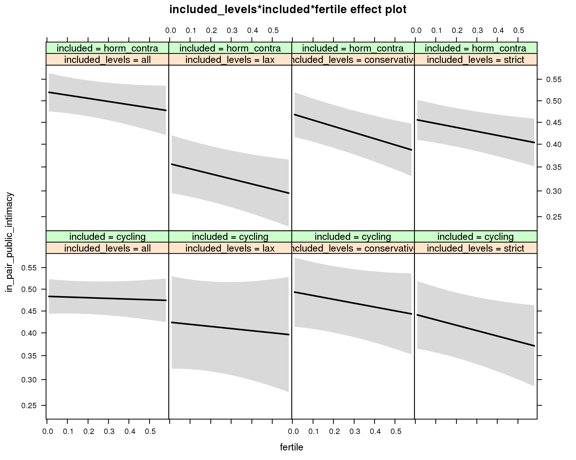
Generalized linear mixed model fit by maximum likelihood (Laplace Approximation) ['glmerMod']
Family: binomial ( probit )
Formula: in_pair_public_intimacy ~ menstruation + fertile_mean + (1 |
person) + included_levels + included + fertile + menstruation:included +
included_levels:included + included_levels:fertile + included:fertile +
included_levels:included:fertile
Data: diary
AIC BIC logLik deviance df.resid
33035 33215 -16495 32991 26682
Scaled residuals:
Min 1Q Median 3Q Max
-3.817 -0.780 -0.356 0.857 3.888
Random effects:
Groups Name Variance Std.Dev.
person (Intercept) 0.47 0.686
Number of obs: 26704, groups: person, 1054
Fixed effects:
Estimate Std. Error z value Pr(>|z|)
(Intercept) -0.06643 0.07719 -0.86 0.389
menstruationpre -0.03652 0.04126 -0.88 0.376
menstruationyes 0.02730 0.03903 0.70 0.484
fertile_mean 0.15573 0.32820 0.47 0.635
included_levelslax -0.15031 0.14648 -1.03 0.305
included_levelsconservative 0.02713 0.11447 0.24 0.813
included_levelsstrict -0.10464 0.11264 -0.93 0.353
includedhorm_contra 0.11374 0.07965 1.43 0.153
fertile -0.03972 0.10552 -0.38 0.707
menstruationpre:includedhorm_contra -0.02184 0.05285 -0.41 0.679
menstruationyes:includedhorm_contra -0.10332 0.05112 -2.02 0.043 *
included_levelslax:includedhorm_contra -0.26664 0.17964 -1.48 0.138
included_levelsconservative:includedhorm_contra -0.15479 0.14411 -1.07 0.283
included_levelsstrict:includedhorm_contra -0.05514 0.13949 -0.40 0.693
included_levelslax:fertile -0.08367 0.26367 -0.32 0.751
included_levelsconservative:fertile -0.18279 0.19025 -0.96 0.337
included_levelsstrict:fertile -0.27548 0.19325 -1.43 0.154
includedhorm_contra:fertile -0.14432 0.16076 -0.90 0.369
included_levelslax:includedhorm_contra:fertile -0.02625 0.32015 -0.08 0.935
included_levelsconservative:includedhorm_contra:fertile 0.00711 0.24807 0.03 0.977
included_levelsstrict:includedhorm_contra:fertile 0.22883 0.24620 0.93 0.353
---
Signif. codes: 0 '***' 0.001 '**' 0.01 '*' 0.05 '.' 0.1 ' ' 1
convergence code: 0
Model failed to converge with max|grad| = 0.00521339 (tol = 0.001, component 1)
M_m6: Moderation by cycle length
model %>%
test_moderator("cycle_length_groups", diary, xlevels = 4)| Df | AIC | BIC | logLik | deviance | Chisq | Chi Df | Pr(>Chisq) | |
|---|---|---|---|---|---|---|---|---|
| with_main | 16 | 33036 | 33167 | -16502 | 33004 | NA | NA | NA |
| with_mod | 22 | 33040 | 33220 | -16498 | 32996 | 7.644 | 6 | 0.2654 |
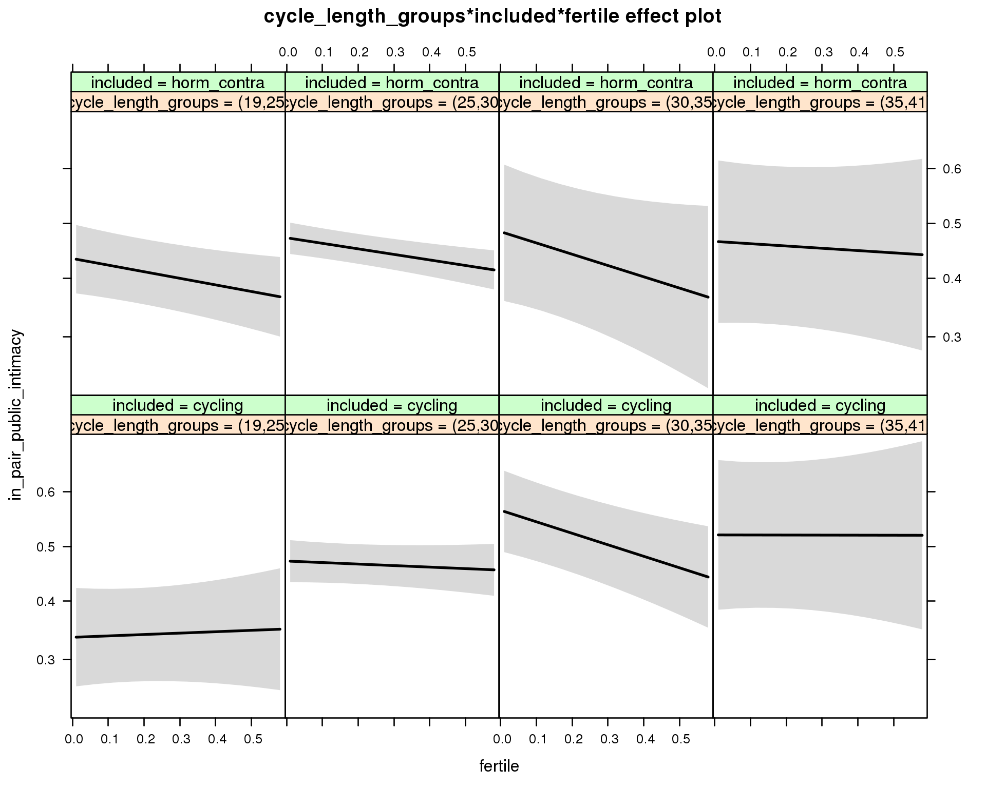
Generalized linear mixed model fit by maximum likelihood (Laplace Approximation) ['glmerMod']
Family: binomial ( probit )
Formula: in_pair_public_intimacy ~ menstruation + fertile_mean + (1 |
person) + cycle_length_groups + included + fertile + menstruation:included +
cycle_length_groups:included + cycle_length_groups:fertile +
included:fertile + cycle_length_groups:included:fertile
Data: diary
AIC BIC logLik deviance df.resid
33040 33220 -16498 32996 26682
Scaled residuals:
Min 1Q Median 3Q Max
-3.902 -0.782 -0.355 0.860 4.137
Random effects:
Groups Name Variance Std.Dev.
person (Intercept) 0.477 0.69
Number of obs: 26704, groups: person, 1054
Fixed effects:
Estimate Std. Error z value Pr(>|z|)
(Intercept) -0.4590 0.1305 -3.52 0.00044 ***
menstruationpre -0.0350 0.0413 -0.85 0.39681
menstruationyes 0.0257 0.0393 0.65 0.51314
fertile_mean 0.2273 0.3292 0.69 0.48993
cycle_length_groups(25,30] 0.3534 0.1269 2.79 0.00535 **
cycle_length_groups(30,35] 0.5885 0.1515 3.88 0.00010 ***
cycle_length_groups(35,41] 0.4746 0.2125 2.23 0.02556 *
includedhorm_contra 0.2796 0.1441 1.94 0.05235 .
fertile 0.0647 0.2274 0.28 0.77617
menstruationpre:includedhorm_contra -0.0232 0.0529 -0.44 0.66112
menstruationyes:includedhorm_contra -0.0985 0.0514 -1.92 0.05514 .
cycle_length_groups(25,30]:includedhorm_contra -0.2572 0.1551 -1.66 0.09728 .
cycle_length_groups(30,35]:includedhorm_contra -0.4641 0.2360 -1.97 0.04928 *
cycle_length_groups(35,41]:includedhorm_contra -0.3951 0.2978 -1.33 0.18455
cycle_length_groups(25,30]:fertile -0.1349 0.2429 -0.56 0.57862
cycle_length_groups(30,35]:fertile -0.5974 0.2870 -2.08 0.03739 *
cycle_length_groups(35,41]:fertile -0.0676 0.3899 -0.17 0.86236
includedhorm_contra:fertile -0.3700 0.2658 -1.39 0.16381
cycle_length_groups(25,30]:includedhorm_contra:fertile 0.1836 0.2851 0.64 0.51958
cycle_length_groups(30,35]:includedhorm_contra:fertile 0.3802 0.4548 0.84 0.40321
cycle_length_groups(35,41]:includedhorm_contra:fertile 0.2669 0.5101 0.52 0.60078
---
Signif. codes: 0 '***' 0.001 '**' 0.01 '*' 0.05 '.' 0.1 ' ' 1
convergence code: 0
Model failed to converge with max|grad| = 0.0120683 (tol = 0.001, component 1)
M_m7: Moderation by certainty about menstruation parameters
model %>%
test_moderator("certainty_menstruation", diary)| Df | AIC | BIC | logLik | deviance | Chisq | Chi Df | Pr(>Chisq) | |
|---|---|---|---|---|---|---|---|---|
| with_main | 12 | 33039 | 33137 | -16507 | 33015 | NA | NA | NA |
| with_mod | 14 | 33041 | 33156 | -16507 | 33013 | 1.55 | 2 | 0.4607 |
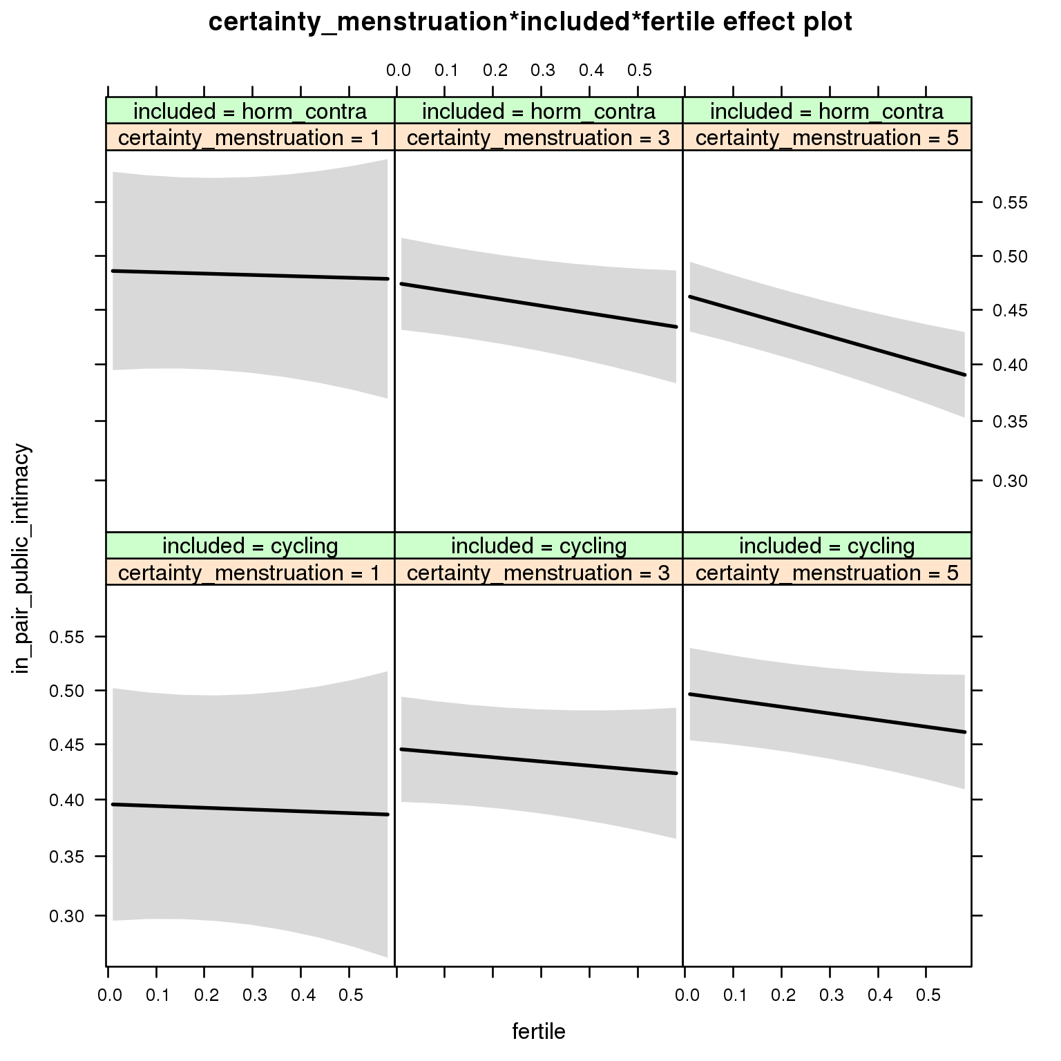
Generalized linear mixed model fit by maximum likelihood (Laplace Approximation) ['glmerMod']
Family: binomial ( probit )
Formula: in_pair_public_intimacy ~ menstruation + fertile_mean + (1 |
person) + certainty_menstruation + included + fertile + menstruation:included +
certainty_menstruation:included + certainty_menstruation:fertile +
included:fertile + certainty_menstruation:included:fertile
Data: diary
AIC BIC logLik deviance df.resid
33041 33156 -16507 33013 26690
Scaled residuals:
Min 1Q Median 3Q Max
-3.781 -0.781 -0.356 0.861 3.972
Random effects:
Groups Name Variance Std.Dev.
person (Intercept) 0.482 0.694
Number of obs: 26704, groups: person, 1054
Fixed effects:
Estimate Std. Error z value Pr(>|z|)
(Intercept) -0.3531 0.1872 -1.89 0.059 .
menstruationpre -0.0358 0.0413 -0.87 0.385
menstruationyes 0.0278 0.0391 0.71 0.478
fertile_mean 0.1453 0.3281 0.44 0.658
certainty_menstruation 0.0646 0.0426 1.52 0.129
includedhorm_contra 0.3307 0.2367 1.40 0.162
fertile -0.0129 0.3292 -0.04 0.969
menstruationpre:includedhorm_contra -0.0235 0.0528 -0.44 0.656
menstruationyes:includedhorm_contra -0.1033 0.0511 -2.02 0.043 *
certainty_menstruation:includedhorm_contra -0.0788 0.0550 -1.43 0.152
certainty_menstruation:fertile -0.0284 0.0771 -0.37 0.712
includedhorm_contra:fertile 0.0524 0.4246 0.12 0.902
certainty_menstruation:includedhorm_contra:fertile -0.0434 0.0982 -0.44 0.658
---
Signif. codes: 0 '***' 0.001 '**' 0.01 '*' 0.05 '.' 0.1 ' ' 1
convergence code: 0
Model failed to converge with max|grad| = 0.109364 (tol = 0.001, component 1)
M_m8: Moderation by cycle regularity
model %>%
test_moderator("cycle_regularity", diary)| Df | AIC | BIC | logLik | deviance | Chisq | Chi Df | Pr(>Chisq) | |
|---|---|---|---|---|---|---|---|---|
| with_main | 14 | 33044 | 33159 | -16508 | 33016 | NA | NA | NA |
| with_mod | 18 | 33048 | 33196 | -16506 | 33012 | 4.097 | 4 | 0.393 |
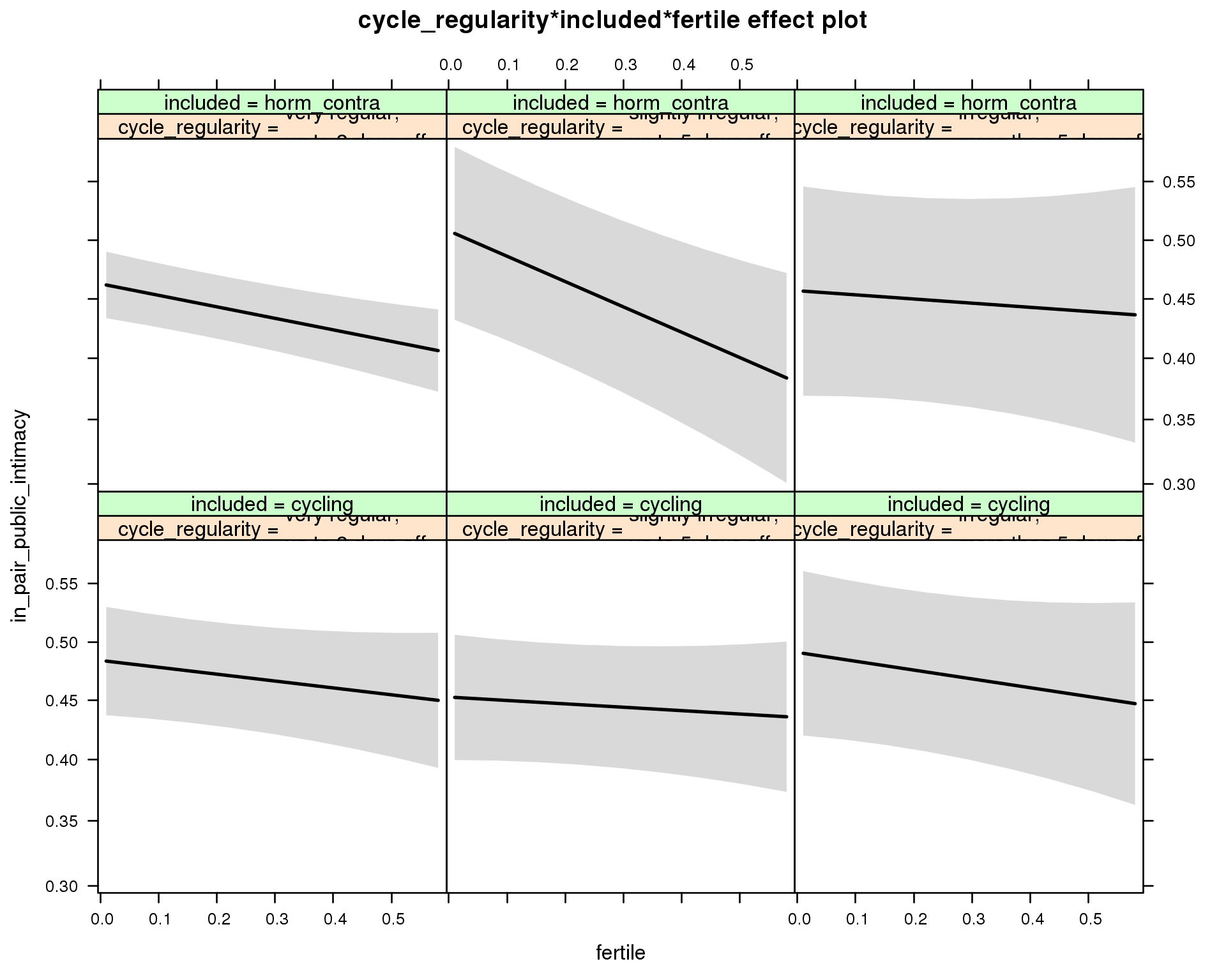
Generalized linear mixed model fit by maximum likelihood (Laplace Approximation) ['glmerMod']
Family: binomial ( probit )
Formula: in_pair_public_intimacy ~ menstruation + fertile_mean + (1 |
person) + cycle_regularity + included + fertile + menstruation:included +
cycle_regularity:included + cycle_regularity:fertile + included:fertile +
cycle_regularity:included:fertile
Data: diary
AIC BIC logLik deviance df.resid
33048 33196 -16506 33012 26686
Scaled residuals:
Min 1Q Median 3Q Max
-3.853 -0.783 -0.355 0.860 3.983
Random effects:
Groups Name Variance Std.Dev.
person (Intercept) 0.482 0.695
Number of obs: 26704, groups: person, 1054
Fixed effects:
Estimate Std. Error z value
(Intercept) -0.0679 0.0821 -0.83
menstruationpre -0.0345 0.0413 -0.84
menstruationyes 0.0291 0.0391 0.74
fertile_mean 0.1686 0.3280 0.51
cycle_regularityslightly irregular,\nup to 5 days off -0.0789 0.0907 -0.87
cycle_regularityirregular,\nmore than 5 days off 0.0172 0.1081 0.16
includedhorm_contra -0.0313 0.0738 -0.42
fertile -0.1481 0.1170 -1.26
menstruationpre:includedhorm_contra -0.0254 0.0528 -0.48
menstruationyes:includedhorm_contra -0.1048 0.0511 -2.05
cycle_regularityslightly irregular,\nup to 5 days off:includedhorm_contra 0.1926 0.1366 1.41
cycle_regularityirregular,\nmore than 5 days off:includedhorm_contra -0.0320 0.1622 -0.20
cycle_regularityslightly irregular,\nup to 5 days off:fertile 0.0750 0.1591 0.47
cycle_regularityirregular,\nmore than 5 days off:fertile -0.0419 0.1962 -0.21
includedhorm_contra:fertile -0.0997 0.1364 -0.73
cycle_regularityslightly irregular,\nup to 5 days off:includedhorm_contra:fertile -0.3726 0.2371 -1.57
cycle_regularityirregular,\nmore than 5 days off:includedhorm_contra:fertile 0.2002 0.2888 0.69
Pr(>|z|)
(Intercept) 0.41
menstruationpre 0.40
menstruationyes 0.46
fertile_mean 0.61
cycle_regularityslightly irregular,\nup to 5 days off 0.38
cycle_regularityirregular,\nmore than 5 days off 0.87
includedhorm_contra 0.67
fertile 0.21
menstruationpre:includedhorm_contra 0.63
menstruationyes:includedhorm_contra 0.04 *
cycle_regularityslightly irregular,\nup to 5 days off:includedhorm_contra 0.16
cycle_regularityirregular,\nmore than 5 days off:includedhorm_contra 0.84
cycle_regularityslightly irregular,\nup to 5 days off:fertile 0.64
cycle_regularityirregular,\nmore than 5 days off:fertile 0.83
includedhorm_contra:fertile 0.46
cycle_regularityslightly irregular,\nup to 5 days off:includedhorm_contra:fertile 0.12
cycle_regularityirregular,\nmore than 5 days off:includedhorm_contra:fertile 0.49
---
Signif. codes: 0 '***' 0.001 '**' 0.01 '*' 0.05 '.' 0.1 ' ' 1
convergence code: 0
Model failed to converge with max|grad| = 0.00267594 (tol = 0.001, component 1)
M_m9: Moderation by cohabitation status
model %>%
test_moderator("cohabitation", diary)| Df | AIC | BIC | logLik | deviance | Chisq | Chi Df | Pr(>Chisq) | |
|---|---|---|---|---|---|---|---|---|
| with_main | 14 | 32841 | 32956 | -16407 | 32813 | NA | NA | NA |
| with_mod | 18 | 32844 | 32992 | -16404 | 32808 | 5.108 | 4 | 0.2764 |
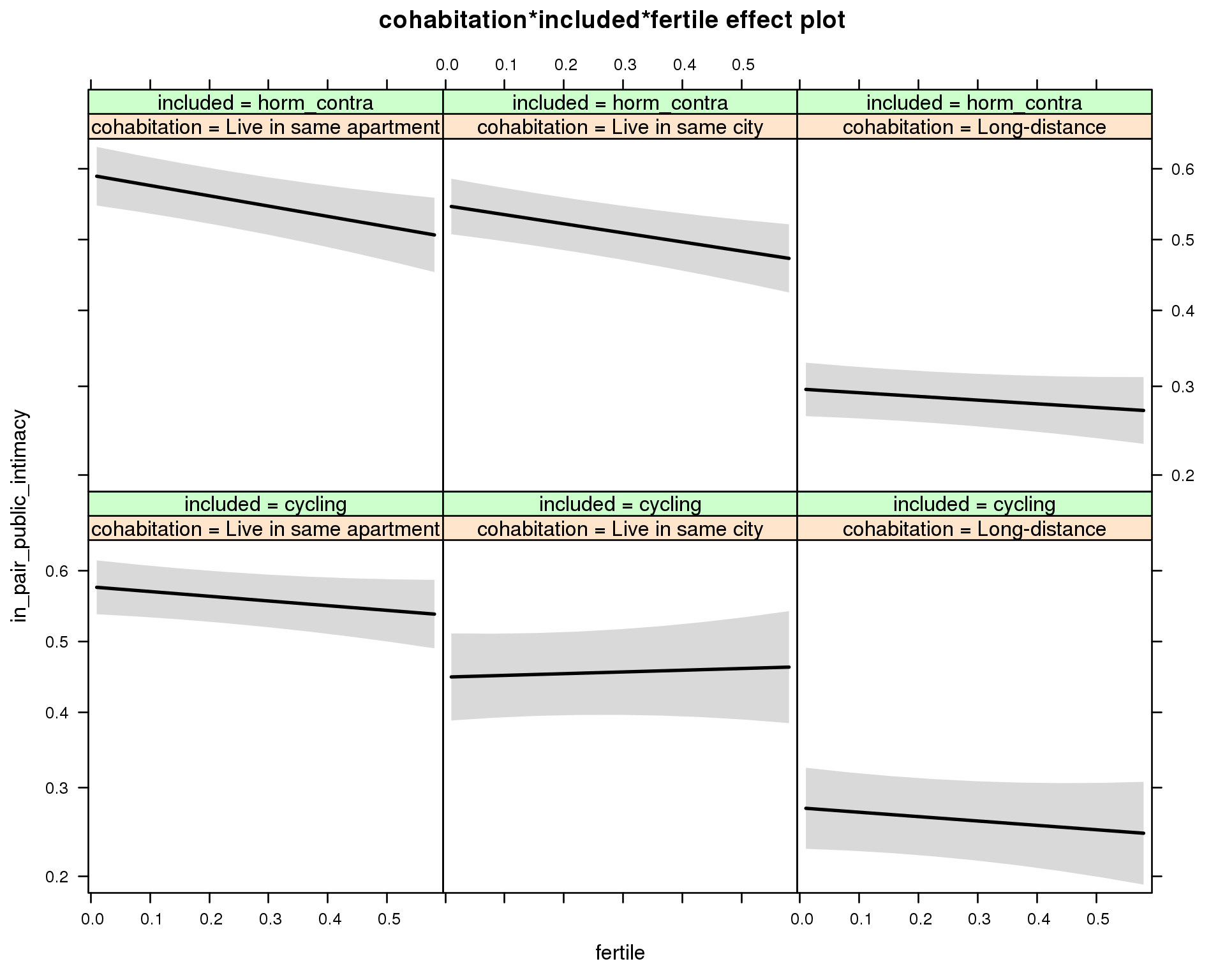
Generalized linear mixed model fit by maximum likelihood (Laplace Approximation) ['glmerMod']
Family: binomial ( probit )
Formula: in_pair_public_intimacy ~ menstruation + fertile_mean + (1 |
person) + cohabitation + included + fertile + menstruation:included +
cohabitation:included + cohabitation:fertile + included:fertile + cohabitation:included:fertile
Data: diary
AIC BIC logLik deviance df.resid
32844 32992 -16404 32808 26686
Scaled residuals:
Min 1Q Median 3Q Max
-3.727 -0.780 -0.358 0.850 4.101
Random effects:
Groups Name Variance Std.Dev.
person (Intercept) 0.368 0.607
Number of obs: 26704, groups: person, 1054
Fixed effects:
Estimate Std. Error z value Pr(>|z|)
(Intercept) 0.1809 0.0728 2.49 0.01295 *
menstruationpre -0.0322 0.0411 -0.78 0.43443
menstruationyes 0.0323 0.0389 0.83 0.40750
fertile_mean 0.0846 0.3007 0.28 0.77832
cohabitationLive in same city -0.3232 0.0934 -3.46 0.00054 ***
cohabitationLong-distance -0.7915 0.0889 -8.91 < 2e-16 ***
includedhorm_contra 0.0572 0.0763 0.75 0.45360
fertile -0.1683 0.1035 -1.63 0.10388
menstruationpre:includedhorm_contra -0.0215 0.0527 -0.41 0.68380
menstruationyes:includedhorm_contra -0.1024 0.0510 -2.01 0.04456 *
cohabitationLive in same city:includedhorm_contra 0.2144 0.1192 1.80 0.07210 .
cohabitationLong-distance:includedhorm_contra 0.0257 0.1147 0.22 0.82278
cohabitationLive in same city:fertile 0.2299 0.1869 1.23 0.21863
cohabitationLong-distance:fertile 0.0118 0.1752 0.07 0.94638
includedhorm_contra:fertile -0.2005 0.1514 -1.32 0.18521
cohabitationLive in same city:includedhorm_contra:fertile -0.1871 0.2343 -0.80 0.42443
cohabitationLong-distance:includedhorm_contra:fertile 0.2249 0.2240 1.00 0.31533
---
Signif. codes: 0 '***' 0.001 '**' 0.01 '*' 0.05 '.' 0.1 ' ' 1
convergence code: 0
Model failed to converge with max|grad| = 0.0146765 (tol = 0.001, component 1)
M_m10: Moderation by relationship status
model %>%
test_moderator("relationship_status_clean", diary)| Df | AIC | BIC | logLik | deviance | Chisq | Chi Df | Pr(>Chisq) | |
|---|---|---|---|---|---|---|---|---|
| with_main | 14 | 33023 | 33138 | -16497 | 32995 | NA | NA | NA |
| with_mod | 18 | 33028 | 33175 | -16496 | 32992 | 3.387 | 4 | 0.4952 |
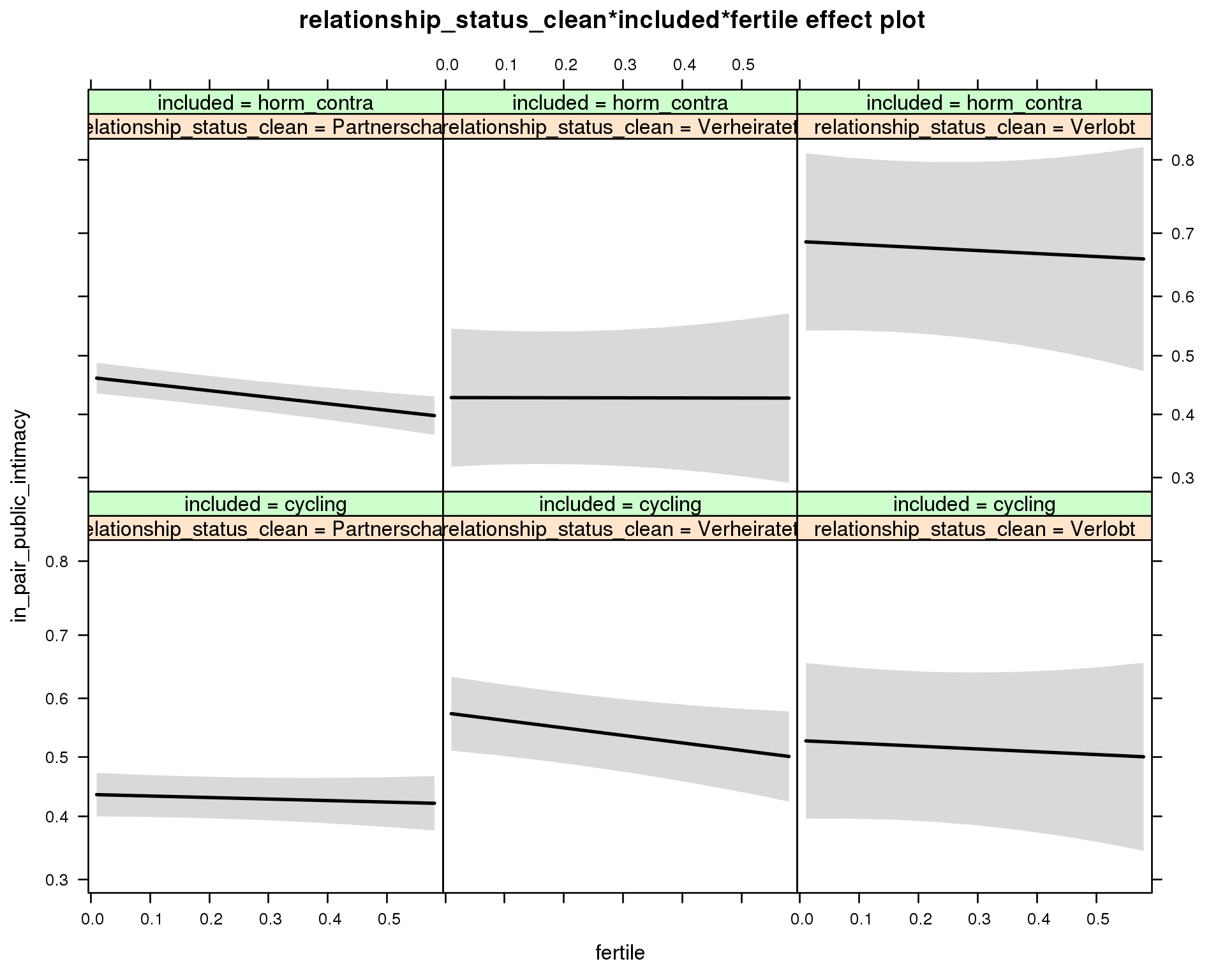
Generalized linear mixed model fit by maximum likelihood (Laplace Approximation) ['glmerMod']
Family: binomial ( probit )
Formula: in_pair_public_intimacy ~ menstruation + fertile_mean + (1 |
person) + relationship_status_clean + included + fertile +
menstruation:included + relationship_status_clean:included +
relationship_status_clean:fertile + included:fertile + relationship_status_clean:included:fertile
Data: diary
AIC BIC logLik deviance df.resid
33028 33175 -16496 32992 26686
Scaled residuals:
Min 1Q Median 3Q Max
-3.761 -0.781 -0.354 0.862 3.979
Random effects:
Groups Name Variance Std.Dev.
person (Intercept) 0.47 0.686
Number of obs: 26704, groups: person, 1054
Fixed effects:
Estimate Std. Error z value Pr(>|z|)
(Intercept) -0.1863 0.0738 -2.52 0.01159 *
menstruationpre -0.0346 0.0412 -0.84 0.40089
menstruationyes 0.0290 0.0390 0.74 0.45821
fertile_mean 0.1589 0.3244 0.49 0.62418
relationship_status_cleanVerheiratet 0.3503 0.0940 3.73 0.00019 ***
relationship_status_cleanVerlobt 0.2315 0.1778 1.30 0.19297
includedhorm_contra 0.0882 0.0629 1.40 0.16113
fertile -0.0651 0.0954 -0.68 0.49491
menstruationpre:includedhorm_contra -0.0249 0.0528 -0.47 0.63674
menstruationyes:includedhorm_contra -0.1039 0.0511 -2.03 0.04191 *
relationship_status_cleanVerheiratet:includedhorm_contra -0.4366 0.1818 -2.40 0.01634 *
relationship_status_cleanVerlobt:includedhorm_contra 0.3522 0.2662 1.32 0.18578
relationship_status_cleanVerheiratet:fertile -0.2572 0.1687 -1.52 0.12727
relationship_status_cleanVerlobt:fertile -0.0547 0.3182 -0.17 0.86341
includedhorm_contra:fertile -0.2173 0.1159 -1.87 0.06091 .
relationship_status_cleanVerheiratet:includedhorm_contra:fertile 0.5357 0.3331 1.61 0.10776
relationship_status_cleanVerlobt:includedhorm_contra:fertile 0.2084 0.4937 0.42 0.67299
---
Signif. codes: 0 '***' 0.001 '**' 0.01 '*' 0.05 '.' 0.1 ' ' 1
convergence code: 0
Model failed to converge with max|grad| = 0.0017076 (tol = 0.001, component 1)
Narcisstic admiration
model_summaries$NARQ_admirationModel summary
Model summary
model %>%
print_summary()Linear mixed model fit by REML
t-tests use Satterthwaite approximations to degrees of freedom ['lmerMod']
Formula: NARQ_admiration ~ included * (menstruation + fertile) + fertile_mean + (1 | person)
Data: diary
REML criterion at convergence: 63018
Scaled residuals:
Min 1Q Median 3Q Max
-5.225 -0.515 -0.073 0.532 5.955
Random effects:
Groups Name Variance Std.Dev.
person (Intercept) 1.139 1.067
Residual 0.535 0.732
Number of obs: 26682, groups: person, 1054
Fixed effects:
Estimate Std. Error df t value Pr(>|t|)
(Intercept) 2.6109 0.0850 1215.0000 30.71 < 2e-16 ***
includedhorm_contra -0.1253 0.0703 1170.0000 -1.78 0.0750 .
menstruationpre -0.0484 0.0224 25788.0000 -2.16 0.0309 *
menstruationyes -0.0997 0.0211 25851.0000 -4.72 0.0000024 ***
fertile -0.0274 0.0452 25793.0000 -0.61 0.5448
fertile_mean 0.2514 0.3830 1290.0000 0.66 0.5118
includedhorm_contra:menstruationpre 0.0394 0.0288 25784.0000 1.37 0.1703
includedhorm_contra:menstruationyes 0.0826 0.0277 25838.0000 2.98 0.0028 **
includedhorm_contra:fertile -0.0188 0.0573 25856.0000 -0.33 0.7432
---
Signif. codes: 0 '***' 0.001 '**' 0.01 '*' 0.05 '.' 0.1 ' ' 1
Correlation of Fixed Effects:
(Intr) incld_ mnstrtnp mnstrtny fertil frtl_m inclddhrm_cntr:mnstrtnp
inclddhrm_c -0.478
menstrutnpr -0.099 0.126
menstrutnys -0.098 0.123 0.399
fertile -0.096 0.158 0.468 0.386
fertile_men -0.769 -0.021 -0.007 -0.005 -0.044
inclddhrm_cntr:mnstrtnp 0.082 -0.158 -0.779 -0.311 -0.364 -0.001
inclddhrm_cntr:mnstrtny 0.078 -0.151 -0.305 -0.763 -0.294 -0.001 0.385
inclddhrm_cntr:f 0.096 -0.199 -0.369 -0.304 -0.787 0.008 0.467
inclddhrm_cntr:mnstrtny
inclddhrm_c
menstrutnpr
menstrutnys
fertile
fertile_men
inclddhrm_cntr:mnstrtnp
inclddhrm_cntr:mnstrtny
inclddhrm_cntr:f 0.382
Effect size standardised by residual variance (\(\frac{b}{ SD_{residual} }\)): -0.04 [-0.16;0.08].
Marginal effect plots
model %>%
plot_all_effects()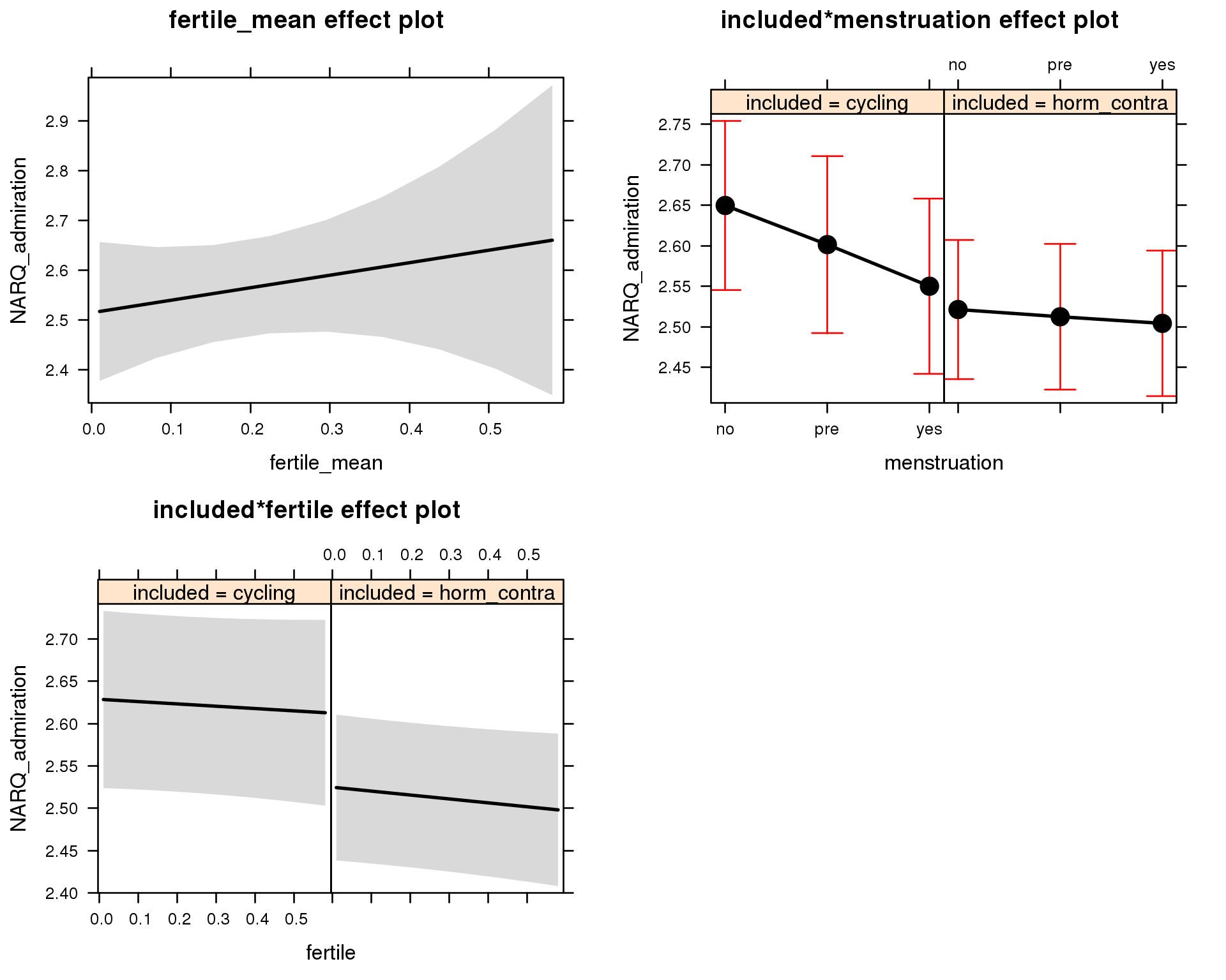
Outcome distribution
model %>%
plot_outcome(diary) + xlab(outcome_label)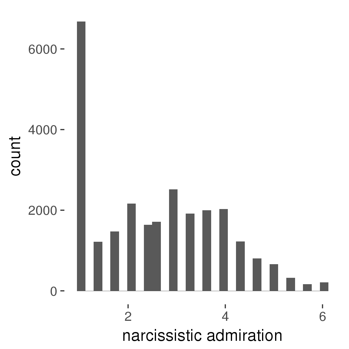
Diagnostics
model %>%
print_diagnostics()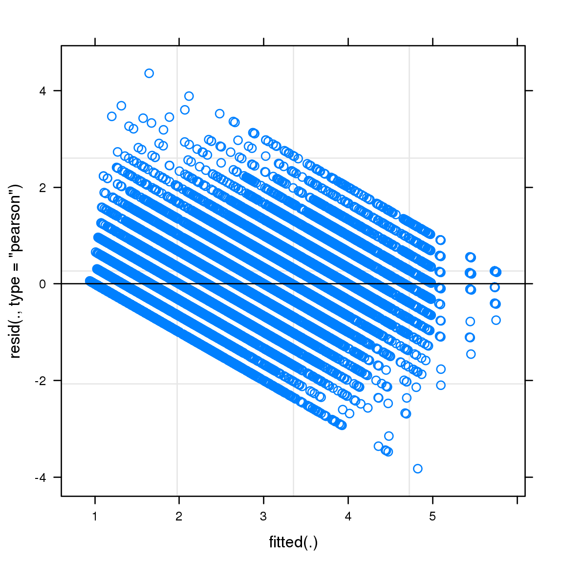
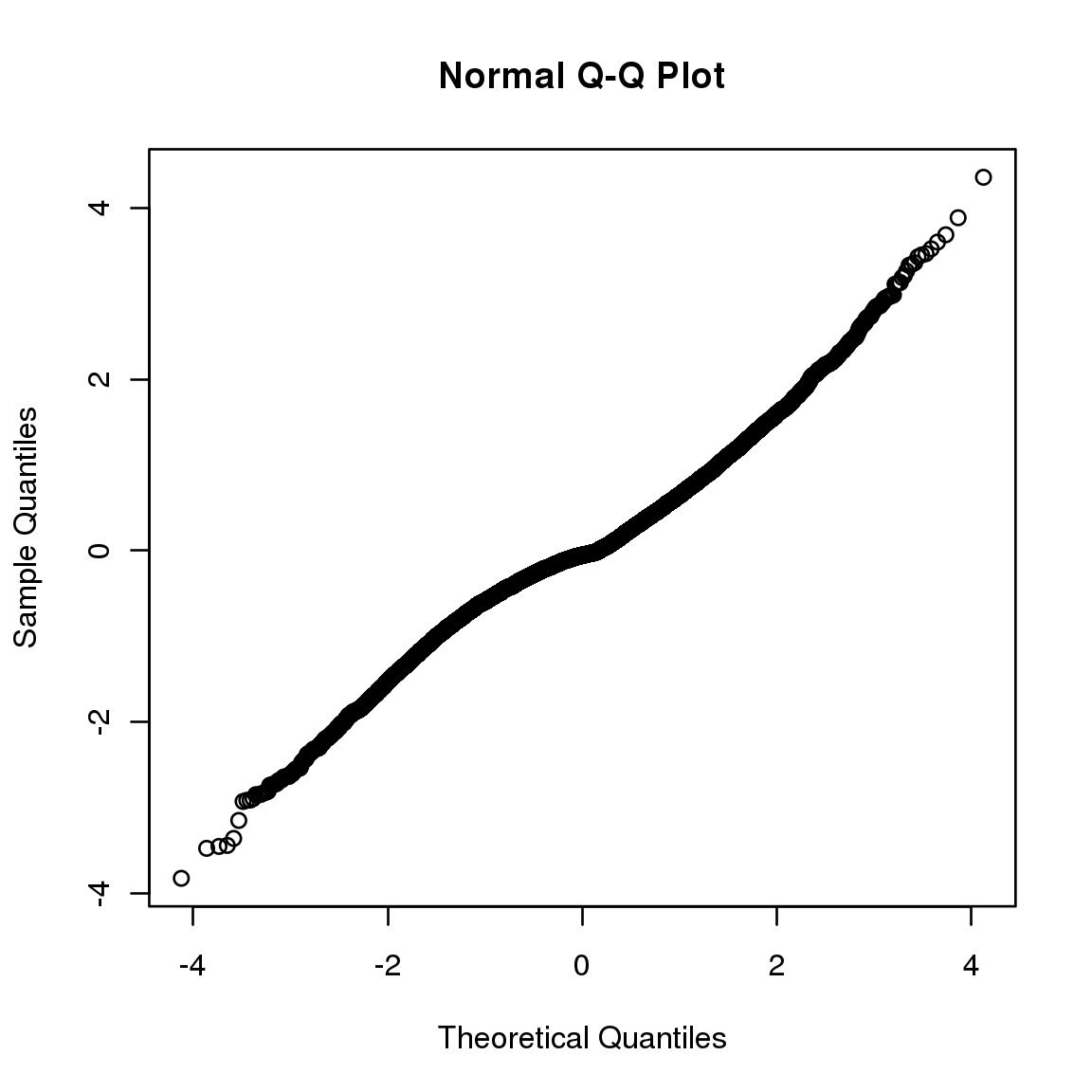
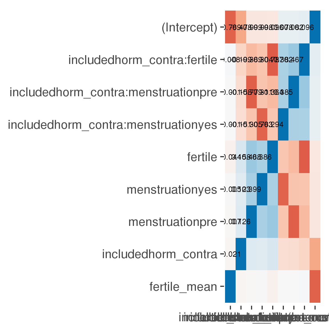
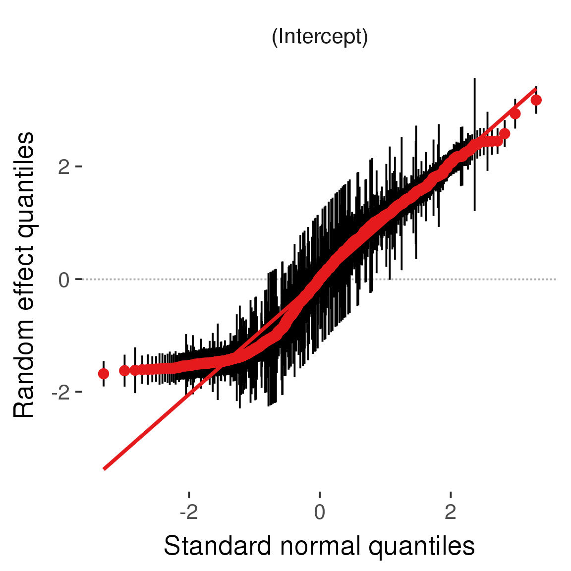
Curves
Here, we continuously plot the outcome over the course of the cycle. Because cycle lengths vary, we subset the data to cycles in a certain range. If the red curve traces the pink curve, our predictor accurately maps the relationship between fertile window probability and the outcome.
Cycle lengths from 21 to 36
Backward-counted
model %>%
plot_curve(diary %>% filter(minimum_cycle_length_diary <= 36, minimum_cycle_length_diary > 20) %>% mutate(fertile=prc_stirn_b))outcome = names(model@frame)[1]
outcome_label = recode(str_replace_all(str_replace_all(str_replace_all(outcome, "_", " "), " pair", "-pair"), " 1", ""),
"desirability 1" = "self-perceived desirability",
"NARQ admiration" = "narcissistic admiration",
"NARQ rivalry" = "narcissistic rivalry",
"extra-pair" = "extra-pair desire & behaviour",
"had sexual intercourse" = "sexual intercourse")
library(ggplot2)
# form a subset and run the model without the hormonal contraception and the fertility predictors
tmp = diary %>%
filter(!is.na(fertile), !is.na(included),
RCD > -1 * minimum_cycle_length_diary, RCD > -40)
new_form = update.formula(formula(model), new = . ~ . - fertile * included)
tmp$residuals = residuals(update(model, new_form, data = tmp , na.action = na.exclude))
tmp = tmp %>%
filter(!is.na(RCD), !is.na(residuals))
rcd_min = min(tmp$RCD)
tmp$real = FALSE
tmp_before = tmp
tmp_before$RCD = tmp_before$RCD + min(tmp$RCD) - 1
tmp_after = tmp
tmp_after$RCD = tmp_after$RCD - min(tmp$RCD) + 1
tmp$real = TRUE
tmp = bind_rows(tmp_before %>% filter(RCD > rcd_min - 11), tmp, tmp_after %>% filter(RCD < 11))GAM smooth on residuals
Here, we partialled out menstruation and individual random effects, then superimposed estimated probability of being in the fertile window scaled to the range of the estimated means. To address the periodicity of the cycle, we prepended and appended ten days of the timeseries to the end and the beginning of the timeseries. We then estimated the GAM and cut off the appended subsets before plotting.
tryCatch({
trend_plot = ggplot(tmp,aes(x = RCD, y = residuals, colour = included)) +
stat_smooth(geom = 'smooth',size = 0.8, fill = "#9ECAE1", method = 'gam', formula = y ~ s(x))
}, error = function(e){cat_message(e, "danger")})
tryCatch({
trend_data = ggplot_build(trend_plot)$data[[1]]
}, error = function(e){cat_message(e, "danger")})
trend_data$RCD = round(trend_data$x)
trend_data = left_join(trend_data, tmp %>% select(real, RCD,fertile) %>% unique(), by = "RCD")
trend_data %>%
filter(real == TRUE) %>%
mutate(superimposed = ( ( (fertile - 0.01)/0.58) * (max(y)-min(y) ) ) + min(y) ) ->
trend_data
ggplot(trend_data) +
geom_ribbon(aes(x = x, ymin = ymin, ymax = ymax, fill = factor(group)), alpha = 0.2) +
geom_line(aes(x = x, y = y, colour = factor(group)), size = 0.8, stat = "identity") +
scale_x_continuous(caption_x) +
geom_line(aes(x = x, y = superimposed), color = "#a83fbf", size = 1, linetype = 'dashed') +
annotate("text",x = mean(trend_data$x), y = max(trend_data$superimposed,na.rm=T) + 0.1, label = 'superimposed fertility peak', color = "#a83fbf") +
scale_y_continuous(outcome_label) +
ggtitle("GAM smooth, residuals") +
scale_color_manual("Contraception status",values = c("2"="black","1"= "red"), labels = c("2"="hormonally\ncontracepting","1"="cycling"), guide = F) +
scale_fill_manual("Contraception status",values = c("2"="black","1"= "red"), labels = c("2"="hormonally\ncontracepting","1"="cycling"), guide = F)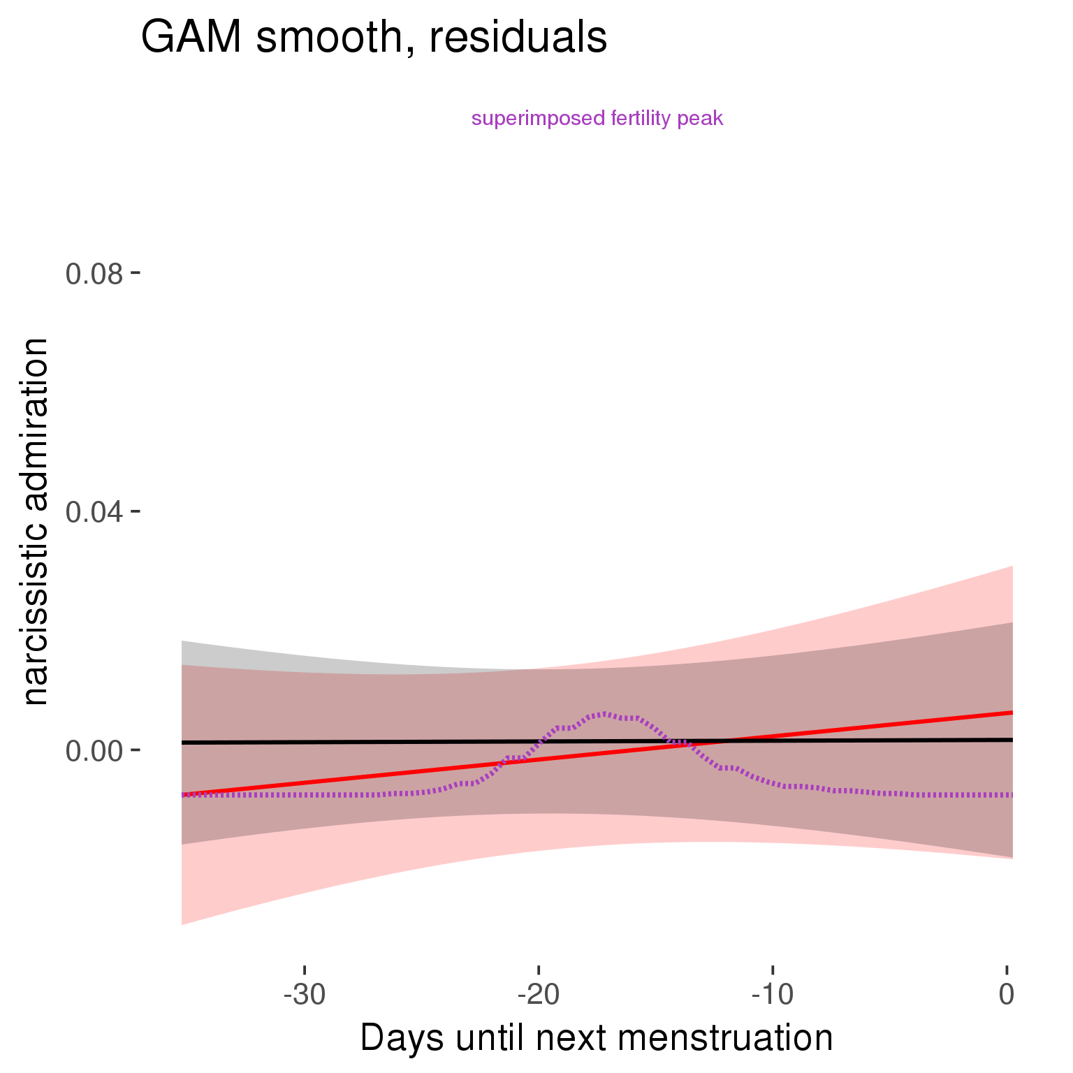
GAM smooth on raw data
As before, but without partialling anything out.
tryCatch({
trend_plot = ggplot(tmp,aes_string(x = "RCD", y = outcome, colour = "included")) +
stat_smooth(geom = 'smooth',size = 0.8, fill = "#9ECAE1", method = 'gam', formula = y ~ s(x))
}, error = function(e){cat_message(e, "danger")})
tryCatch({
trend_data = ggplot_build(trend_plot)$data[[1]]
}, error = function(e){cat_message(e, "danger")})
trend_data$RCD = round(trend_data$x)
trend_data = left_join(trend_data, tmp %>% select(real, RCD,fertile) %>% unique(), by = "RCD")
trend_data %>%
filter(real == TRUE) %>%
mutate(superimposed = ( ( (fertile - 0.01)/0.58) * (max(y)-min(y) ) ) + min(y) ) ->
trend_data
plot1b = ggplot(trend_data) +
geom_ribbon(aes(x = x, ymin = ymin, ymax = ymax, fill = factor(group)), alpha = 0.2) +
geom_line(aes(x = x, y = y, colour = factor(group)), size = 0.8, stat = "identity") +
scale_x_continuous(caption_x) +
geom_line(aes(x = x, y = superimposed), color = "#a83fbf", size = 1, linetype = 'dashed') +
annotate("text",x = mean(trend_data$x), y = max(trend_data$superimposed,na.rm=T) + 0.1, label = 'superimposed fertility peak', color = "#a83fbf") +
scale_y_continuous(outcome_label) +
ggtitle("GAM smooth, raw data") +
scale_color_manual("Contraception status",values = c("2"="black","1"= "red"), labels = c("2"="hormonally\ncontracepting","1"="cycling"), guide = F) +
scale_fill_manual("Contraception status",values = c("2"="black","1"= "red"), labels = c("2"="hormonally\ncontracepting","1"="cycling"), guide = F)
suppressWarnings(print(plot1b))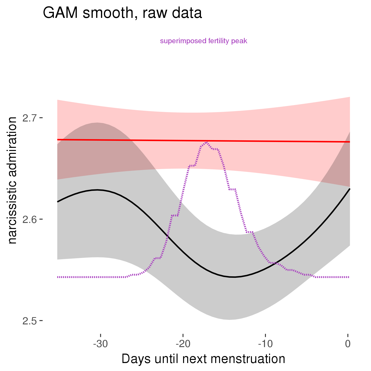
Means and standard errors over raw data
Nothing partialled out, just straight means with bootstrapped confidence intervals.
tryCatch({
trend_plot = ggplot(tmp,aes_string(x = "RCD", y = outcome, colour = "included")) +
geom_pointrange(size = 0.8, stat = 'summary', fun.data = "mean_cl_boot")
}, error = function(e){cat_message(e, "danger")})
tryCatch({
trend_data = ggplot_build(trend_plot)$data[[1]]
}, error = function(e){cat_message(e, "danger")})
trend_data$RCD = round(trend_data$x)
trend_data = left_join(trend_data, tmp %>% select(real, RCD,fertile) %>% unique(), by = "RCD")
trend_data %>%
filter(real == TRUE) %>%
mutate(superimposed = ( ( (fertile - 0.01)/0.58) * (max(y)-min(y) ) ) + min(y) ) ->
trend_data
plot3 = ggplot(trend_data) +
geom_pointrange(aes(x = x, y = y, ymin = ymin,ymax = ymax, colour = factor(group)), size = 0.8, stat = "identity", alpha = 0.6, position = position_dodge(width = .5)) +
scale_x_continuous("Days until next menstruation") +
geom_line(aes(x= x, y = superimposed), color = "#a83fbf", size = 1, linetype = 'dashed') +
annotate("text",x = mean(trend_data$x), y = max(trend_data$superimposed,na.rm=T) + 0.1, label = 'superimposed fertility peak', color = "#a83fbf") +
scale_y_continuous(outcome_label) +
ggtitle("Means with standard errors, raw data") +
scale_color_manual("Contraception status",values = c("2"="black","1"= "red"), labels = c("2"="hormonally\ncontracepting","1"="cycling"), guide = F) +
scale_fill_manual("Contraception status",values = c("2"="black","1"= "red"), labels = c("2"="hormonally\ncontracepting","1"="cycling"), guide = F)
suppressWarnings(print(plot3))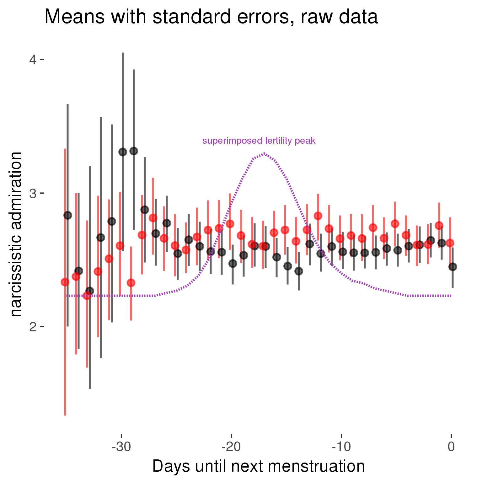
Forward-counted
model %>%
plot_curve(diary %>% filter(minimum_cycle_length_diary <= 36, minimum_cycle_length_diary > 20) %>% mutate(RCD = FCD, fertile = prc_stirn_b_forward_counted), caption_x = "Days since last menstruation")outcome = names(model@frame)[1]
outcome_label = recode(str_replace_all(str_replace_all(str_replace_all(outcome, "_", " "), " pair", "-pair"), " 1", ""),
"desirability 1" = "self-perceived desirability",
"NARQ admiration" = "narcissistic admiration",
"NARQ rivalry" = "narcissistic rivalry",
"extra-pair" = "extra-pair desire & behaviour",
"had sexual intercourse" = "sexual intercourse")
library(ggplot2)
# form a subset and run the model without the hormonal contraception and the fertility predictors
tmp = diary %>%
filter(!is.na(fertile), !is.na(included),
RCD > -1 * minimum_cycle_length_diary, RCD > -40)
new_form = update.formula(formula(model), new = . ~ . - fertile * included)
tmp$residuals = residuals(update(model, new_form, data = tmp , na.action = na.exclude))
tmp = tmp %>%
filter(!is.na(RCD), !is.na(residuals))
rcd_min = min(tmp$RCD)
tmp$real = FALSE
tmp_before = tmp
tmp_before$RCD = tmp_before$RCD + min(tmp$RCD) - 1
tmp_after = tmp
tmp_after$RCD = tmp_after$RCD - min(tmp$RCD) + 1
tmp$real = TRUE
tmp = bind_rows(tmp_before %>% filter(RCD > rcd_min - 11), tmp, tmp_after %>% filter(RCD < 11))GAM smooth on residuals
Here, we partialled out menstruation and individual random effects, then superimposed estimated probability of being in the fertile window scaled to the range of the estimated means. To address the periodicity of the cycle, we prepended and appended ten days of the timeseries to the end and the beginning of the timeseries. We then estimated the GAM and cut off the appended subsets before plotting.
tryCatch({
trend_plot = ggplot(tmp,aes(x = RCD, y = residuals, colour = included)) +
stat_smooth(geom = 'smooth',size = 0.8, fill = "#9ECAE1", method = 'gam', formula = y ~ s(x))
}, error = function(e){cat_message(e, "danger")})
tryCatch({
trend_data = ggplot_build(trend_plot)$data[[1]]
}, error = function(e){cat_message(e, "danger")})
trend_data$RCD = round(trend_data$x)
trend_data = left_join(trend_data, tmp %>% select(real, RCD,fertile) %>% unique(), by = "RCD")
trend_data %>%
filter(real == TRUE) %>%
mutate(superimposed = ( ( (fertile - 0.01)/0.58) * (max(y)-min(y) ) ) + min(y) ) ->
trend_data
ggplot(trend_data) +
geom_ribbon(aes(x = x, ymin = ymin, ymax = ymax, fill = factor(group)), alpha = 0.2) +
geom_line(aes(x = x, y = y, colour = factor(group)), size = 0.8, stat = "identity") +
scale_x_continuous(caption_x) +
geom_line(aes(x = x, y = superimposed), color = "#a83fbf", size = 1, linetype = 'dashed') +
annotate("text",x = mean(trend_data$x), y = max(trend_data$superimposed,na.rm=T) + 0.1, label = 'superimposed fertility peak', color = "#a83fbf") +
scale_y_continuous(outcome_label) +
ggtitle("GAM smooth, residuals") +
scale_color_manual("Contraception status",values = c("2"="black","1"= "red"), labels = c("2"="hormonally\ncontracepting","1"="cycling"), guide = F) +
scale_fill_manual("Contraception status",values = c("2"="black","1"= "red"), labels = c("2"="hormonally\ncontracepting","1"="cycling"), guide = F)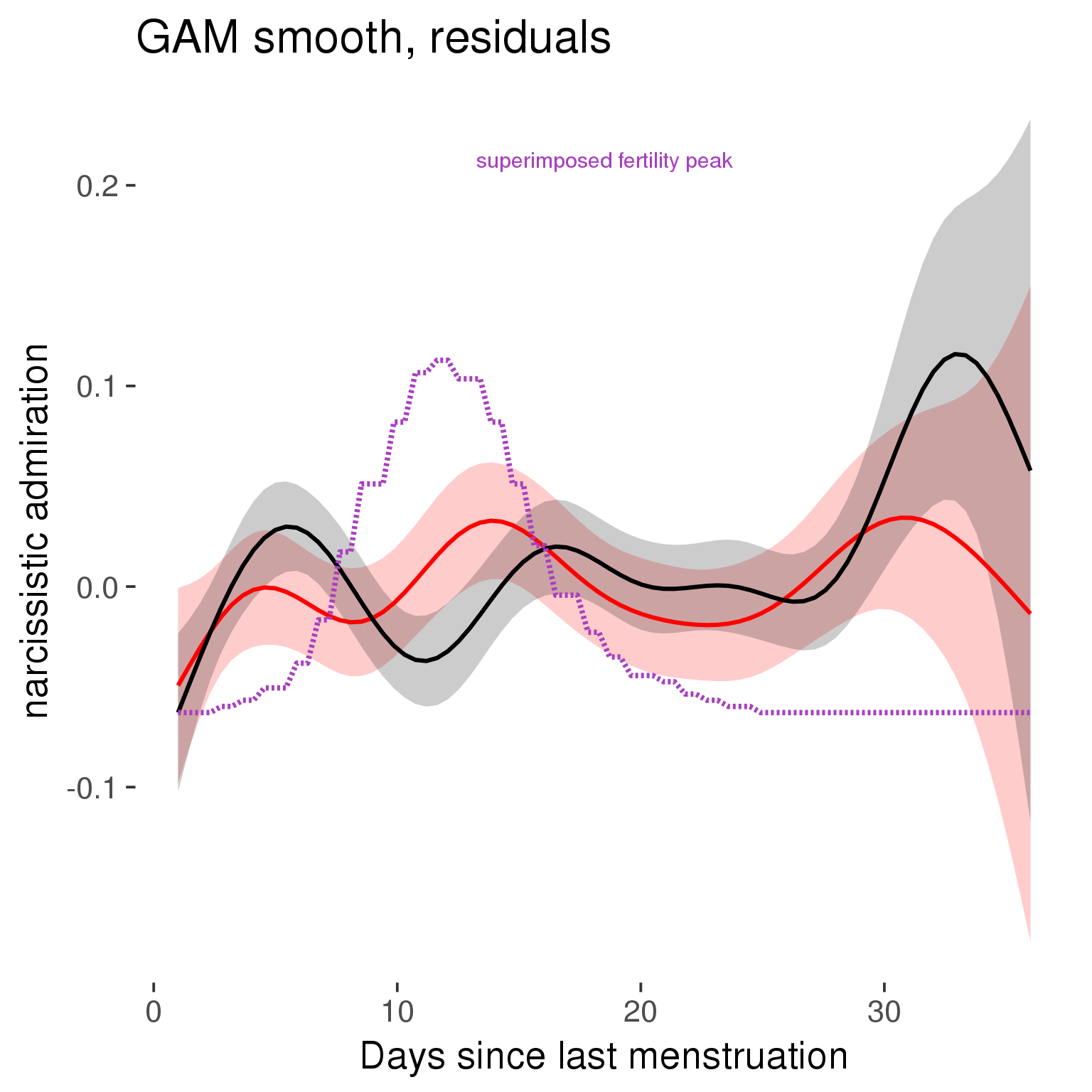
GAM smooth on raw data
As before, but without partialling anything out.
tryCatch({
trend_plot = ggplot(tmp,aes_string(x = "RCD", y = outcome, colour = "included")) +
stat_smooth(geom = 'smooth',size = 0.8, fill = "#9ECAE1", method = 'gam', formula = y ~ s(x))
}, error = function(e){cat_message(e, "danger")})
tryCatch({
trend_data = ggplot_build(trend_plot)$data[[1]]
}, error = function(e){cat_message(e, "danger")})
trend_data$RCD = round(trend_data$x)
trend_data = left_join(trend_data, tmp %>% select(real, RCD,fertile) %>% unique(), by = "RCD")
trend_data %>%
filter(real == TRUE) %>%
mutate(superimposed = ( ( (fertile - 0.01)/0.58) * (max(y)-min(y) ) ) + min(y) ) ->
trend_data
plot1b = ggplot(trend_data) +
geom_ribbon(aes(x = x, ymin = ymin, ymax = ymax, fill = factor(group)), alpha = 0.2) +
geom_line(aes(x = x, y = y, colour = factor(group)), size = 0.8, stat = "identity") +
scale_x_continuous(caption_x) +
geom_line(aes(x = x, y = superimposed), color = "#a83fbf", size = 1, linetype = 'dashed') +
annotate("text",x = mean(trend_data$x), y = max(trend_data$superimposed,na.rm=T) + 0.1, label = 'superimposed fertility peak', color = "#a83fbf") +
scale_y_continuous(outcome_label) +
ggtitle("GAM smooth, raw data") +
scale_color_manual("Contraception status",values = c("2"="black","1"= "red"), labels = c("2"="hormonally\ncontracepting","1"="cycling"), guide = F) +
scale_fill_manual("Contraception status",values = c("2"="black","1"= "red"), labels = c("2"="hormonally\ncontracepting","1"="cycling"), guide = F)
suppressWarnings(print(plot1b))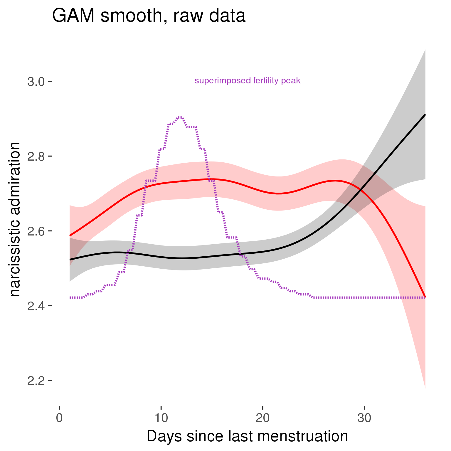
Means and standard errors over raw data
Nothing partialled out, just straight means with bootstrapped confidence intervals.
tryCatch({
trend_plot = ggplot(tmp,aes_string(x = "RCD", y = outcome, colour = "included")) +
geom_pointrange(size = 0.8, stat = 'summary', fun.data = "mean_cl_boot")
}, error = function(e){cat_message(e, "danger")})
tryCatch({
trend_data = ggplot_build(trend_plot)$data[[1]]
}, error = function(e){cat_message(e, "danger")})
trend_data$RCD = round(trend_data$x)
trend_data = left_join(trend_data, tmp %>% select(real, RCD,fertile) %>% unique(), by = "RCD")
trend_data %>%
filter(real == TRUE) %>%
mutate(superimposed = ( ( (fertile - 0.01)/0.58) * (max(y)-min(y) ) ) + min(y) ) ->
trend_data
plot3 = ggplot(trend_data) +
geom_pointrange(aes(x = x, y = y, ymin = ymin,ymax = ymax, colour = factor(group)), size = 0.8, stat = "identity", alpha = 0.6, position = position_dodge(width = .5)) +
scale_x_continuous("Days until next menstruation") +
geom_line(aes(x= x, y = superimposed), color = "#a83fbf", size = 1, linetype = 'dashed') +
annotate("text",x = mean(trend_data$x), y = max(trend_data$superimposed,na.rm=T) + 0.1, label = 'superimposed fertility peak', color = "#a83fbf") +
scale_y_continuous(outcome_label) +
ggtitle("Means with standard errors, raw data") +
scale_color_manual("Contraception status",values = c("2"="black","1"= "red"), labels = c("2"="hormonally\ncontracepting","1"="cycling"), guide = F) +
scale_fill_manual("Contraception status",values = c("2"="black","1"= "red"), labels = c("2"="hormonally\ncontracepting","1"="cycling"), guide = F)
suppressWarnings(print(plot3))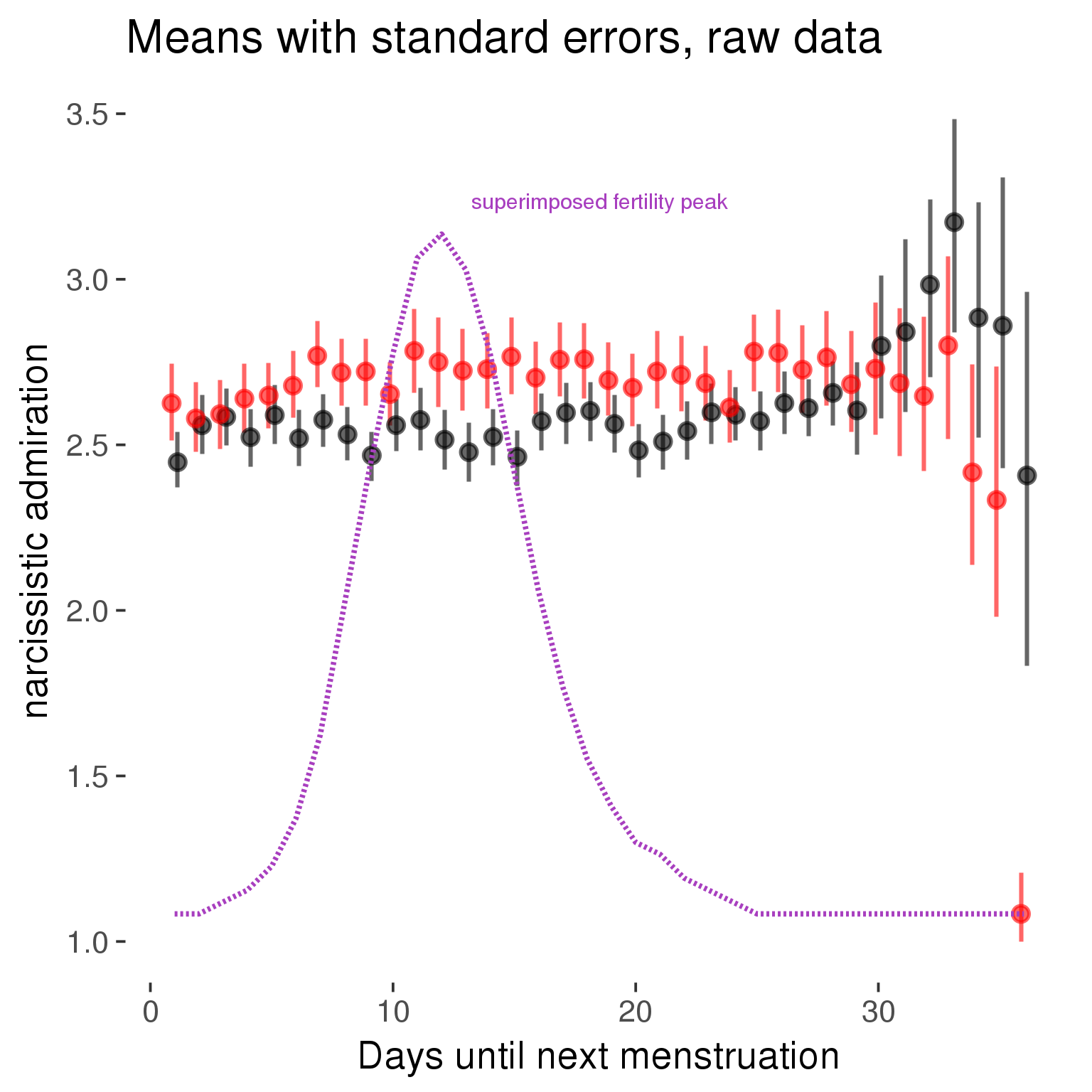
Cycle lengths from 27 to 30
Backward-counted
model %>%
plot_curve(diary %>% filter(minimum_cycle_length_diary <= 30, minimum_cycle_length_diary >= 27) %>% mutate(fertile=prc_stirn_b))outcome = names(model@frame)[1]
outcome_label = recode(str_replace_all(str_replace_all(str_replace_all(outcome, "_", " "), " pair", "-pair"), " 1", ""),
"desirability 1" = "self-perceived desirability",
"NARQ admiration" = "narcissistic admiration",
"NARQ rivalry" = "narcissistic rivalry",
"extra-pair" = "extra-pair desire & behaviour",
"had sexual intercourse" = "sexual intercourse")
library(ggplot2)
# form a subset and run the model without the hormonal contraception and the fertility predictors
tmp = diary %>%
filter(!is.na(fertile), !is.na(included),
RCD > -1 * minimum_cycle_length_diary, RCD > -40)
new_form = update.formula(formula(model), new = . ~ . - fertile * included)
tmp$residuals = residuals(update(model, new_form, data = tmp , na.action = na.exclude))
tmp = tmp %>%
filter(!is.na(RCD), !is.na(residuals))
rcd_min = min(tmp$RCD)
tmp$real = FALSE
tmp_before = tmp
tmp_before$RCD = tmp_before$RCD + min(tmp$RCD) - 1
tmp_after = tmp
tmp_after$RCD = tmp_after$RCD - min(tmp$RCD) + 1
tmp$real = TRUE
tmp = bind_rows(tmp_before %>% filter(RCD > rcd_min - 11), tmp, tmp_after %>% filter(RCD < 11))GAM smooth on residuals
Here, we partialled out menstruation and individual random effects, then superimposed estimated probability of being in the fertile window scaled to the range of the estimated means. To address the periodicity of the cycle, we prepended and appended ten days of the timeseries to the end and the beginning of the timeseries. We then estimated the GAM and cut off the appended subsets before plotting.
tryCatch({
trend_plot = ggplot(tmp,aes(x = RCD, y = residuals, colour = included)) +
stat_smooth(geom = 'smooth',size = 0.8, fill = "#9ECAE1", method = 'gam', formula = y ~ s(x))
}, error = function(e){cat_message(e, "danger")})
tryCatch({
trend_data = ggplot_build(trend_plot)$data[[1]]
}, error = function(e){cat_message(e, "danger")})
trend_data$RCD = round(trend_data$x)
trend_data = left_join(trend_data, tmp %>% select(real, RCD,fertile) %>% unique(), by = "RCD")
trend_data %>%
filter(real == TRUE) %>%
mutate(superimposed = ( ( (fertile - 0.01)/0.58) * (max(y)-min(y) ) ) + min(y) ) ->
trend_data
ggplot(trend_data) +
geom_ribbon(aes(x = x, ymin = ymin, ymax = ymax, fill = factor(group)), alpha = 0.2) +
geom_line(aes(x = x, y = y, colour = factor(group)), size = 0.8, stat = "identity") +
scale_x_continuous(caption_x) +
geom_line(aes(x = x, y = superimposed), color = "#a83fbf", size = 1, linetype = 'dashed') +
annotate("text",x = mean(trend_data$x), y = max(trend_data$superimposed,na.rm=T) + 0.1, label = 'superimposed fertility peak', color = "#a83fbf") +
scale_y_continuous(outcome_label) +
ggtitle("GAM smooth, residuals") +
scale_color_manual("Contraception status",values = c("2"="black","1"= "red"), labels = c("2"="hormonally\ncontracepting","1"="cycling"), guide = F) +
scale_fill_manual("Contraception status",values = c("2"="black","1"= "red"), labels = c("2"="hormonally\ncontracepting","1"="cycling"), guide = F)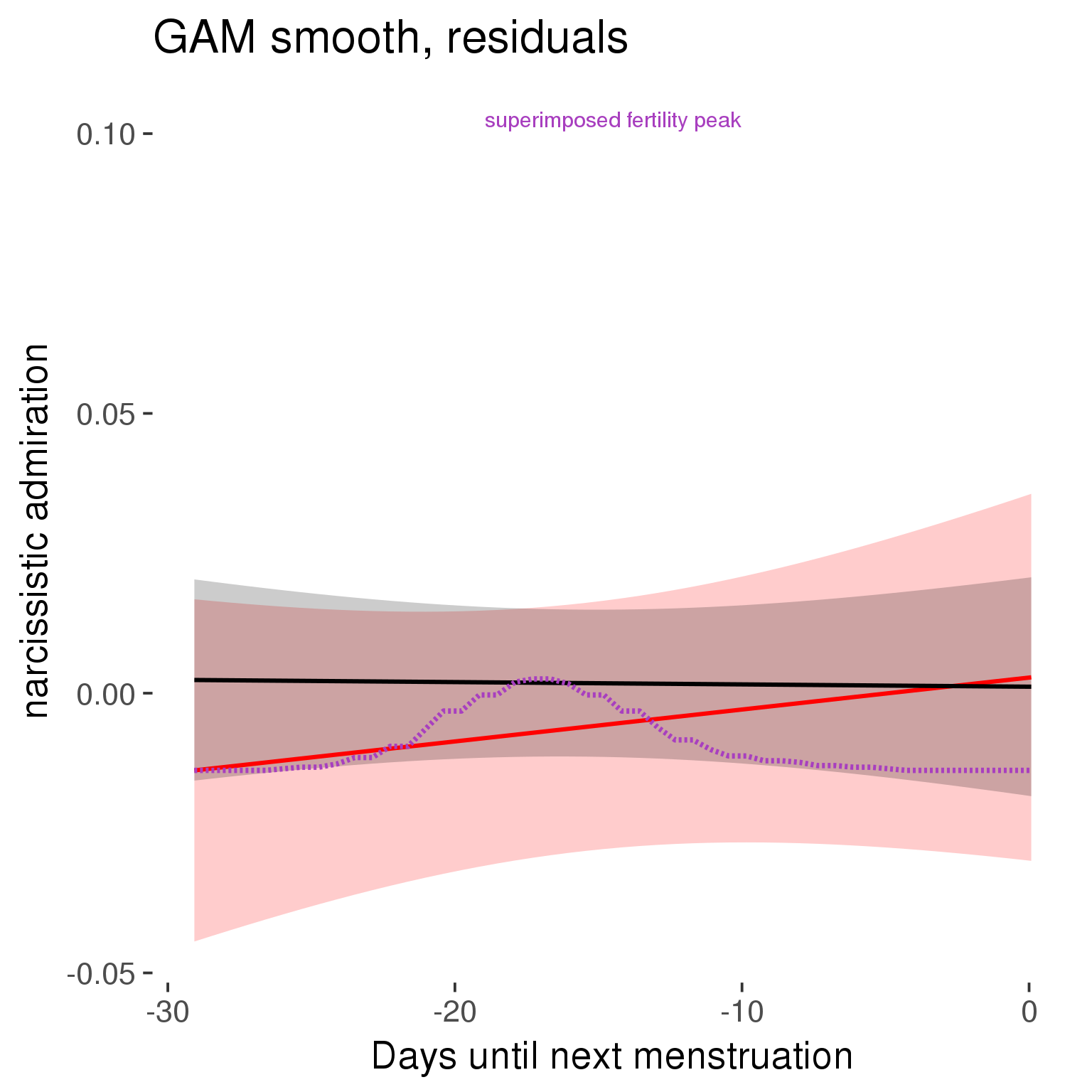
GAM smooth on raw data
As before, but without partialling anything out.
tryCatch({
trend_plot = ggplot(tmp,aes_string(x = "RCD", y = outcome, colour = "included")) +
stat_smooth(geom = 'smooth',size = 0.8, fill = "#9ECAE1", method = 'gam', formula = y ~ s(x))
}, error = function(e){cat_message(e, "danger")})
tryCatch({
trend_data = ggplot_build(trend_plot)$data[[1]]
}, error = function(e){cat_message(e, "danger")})
trend_data$RCD = round(trend_data$x)
trend_data = left_join(trend_data, tmp %>% select(real, RCD,fertile) %>% unique(), by = "RCD")
trend_data %>%
filter(real == TRUE) %>%
mutate(superimposed = ( ( (fertile - 0.01)/0.58) * (max(y)-min(y) ) ) + min(y) ) ->
trend_data
plot1b = ggplot(trend_data) +
geom_ribbon(aes(x = x, ymin = ymin, ymax = ymax, fill = factor(group)), alpha = 0.2) +
geom_line(aes(x = x, y = y, colour = factor(group)), size = 0.8, stat = "identity") +
scale_x_continuous(caption_x) +
geom_line(aes(x = x, y = superimposed), color = "#a83fbf", size = 1, linetype = 'dashed') +
annotate("text",x = mean(trend_data$x), y = max(trend_data$superimposed,na.rm=T) + 0.1, label = 'superimposed fertility peak', color = "#a83fbf") +
scale_y_continuous(outcome_label) +
ggtitle("GAM smooth, raw data") +
scale_color_manual("Contraception status",values = c("2"="black","1"= "red"), labels = c("2"="hormonally\ncontracepting","1"="cycling"), guide = F) +
scale_fill_manual("Contraception status",values = c("2"="black","1"= "red"), labels = c("2"="hormonally\ncontracepting","1"="cycling"), guide = F)
suppressWarnings(print(plot1b))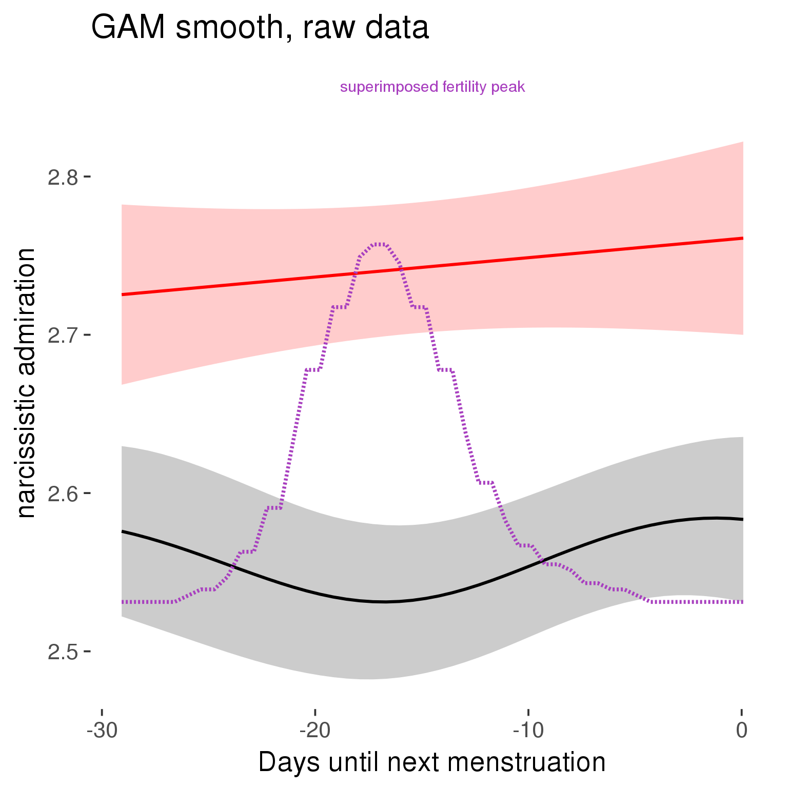
Means and standard errors over raw data
Nothing partialled out, just straight means with bootstrapped confidence intervals.
tryCatch({
trend_plot = ggplot(tmp,aes_string(x = "RCD", y = outcome, colour = "included")) +
geom_pointrange(size = 0.8, stat = 'summary', fun.data = "mean_cl_boot")
}, error = function(e){cat_message(e, "danger")})
tryCatch({
trend_data = ggplot_build(trend_plot)$data[[1]]
}, error = function(e){cat_message(e, "danger")})
trend_data$RCD = round(trend_data$x)
trend_data = left_join(trend_data, tmp %>% select(real, RCD,fertile) %>% unique(), by = "RCD")
trend_data %>%
filter(real == TRUE) %>%
mutate(superimposed = ( ( (fertile - 0.01)/0.58) * (max(y)-min(y) ) ) + min(y) ) ->
trend_data
plot3 = ggplot(trend_data) +
geom_pointrange(aes(x = x, y = y, ymin = ymin,ymax = ymax, colour = factor(group)), size = 0.8, stat = "identity", alpha = 0.6, position = position_dodge(width = .5)) +
scale_x_continuous("Days until next menstruation") +
geom_line(aes(x= x, y = superimposed), color = "#a83fbf", size = 1, linetype = 'dashed') +
annotate("text",x = mean(trend_data$x), y = max(trend_data$superimposed,na.rm=T) + 0.1, label = 'superimposed fertility peak', color = "#a83fbf") +
scale_y_continuous(outcome_label) +
ggtitle("Means with standard errors, raw data") +
scale_color_manual("Contraception status",values = c("2"="black","1"= "red"), labels = c("2"="hormonally\ncontracepting","1"="cycling"), guide = F) +
scale_fill_manual("Contraception status",values = c("2"="black","1"= "red"), labels = c("2"="hormonally\ncontracepting","1"="cycling"), guide = F)
suppressWarnings(print(plot3))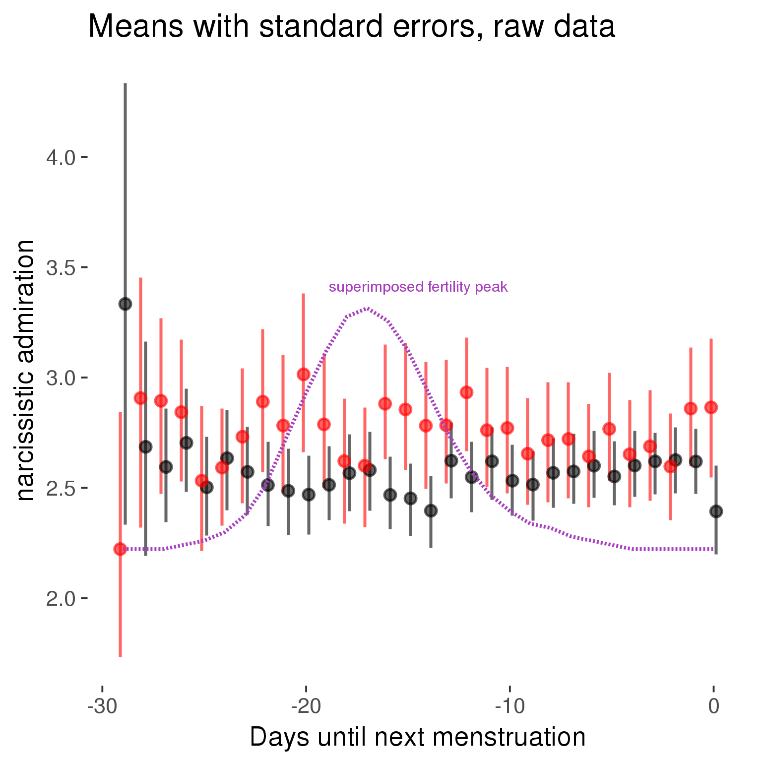
Forward-counted
model %>%
plot_curve(diary %>% filter(minimum_cycle_length_diary <= 30, minimum_cycle_length_diary >= 27) %>% mutate(RCD = FCD, fertile = prc_stirn_b_forward_counted), caption_x = "Days since last menstruation")outcome = names(model@frame)[1]
outcome_label = recode(str_replace_all(str_replace_all(str_replace_all(outcome, "_", " "), " pair", "-pair"), " 1", ""),
"desirability 1" = "self-perceived desirability",
"NARQ admiration" = "narcissistic admiration",
"NARQ rivalry" = "narcissistic rivalry",
"extra-pair" = "extra-pair desire & behaviour",
"had sexual intercourse" = "sexual intercourse")
library(ggplot2)
# form a subset and run the model without the hormonal contraception and the fertility predictors
tmp = diary %>%
filter(!is.na(fertile), !is.na(included),
RCD > -1 * minimum_cycle_length_diary, RCD > -40)
new_form = update.formula(formula(model), new = . ~ . - fertile * included)
tmp$residuals = residuals(update(model, new_form, data = tmp , na.action = na.exclude))
tmp = tmp %>%
filter(!is.na(RCD), !is.na(residuals))
rcd_min = min(tmp$RCD)
tmp$real = FALSE
tmp_before = tmp
tmp_before$RCD = tmp_before$RCD + min(tmp$RCD) - 1
tmp_after = tmp
tmp_after$RCD = tmp_after$RCD - min(tmp$RCD) + 1
tmp$real = TRUE
tmp = bind_rows(tmp_before %>% filter(RCD > rcd_min - 11), tmp, tmp_after %>% filter(RCD < 11))GAM smooth on residuals
Here, we partialled out menstruation and individual random effects, then superimposed estimated probability of being in the fertile window scaled to the range of the estimated means. To address the periodicity of the cycle, we prepended and appended ten days of the timeseries to the end and the beginning of the timeseries. We then estimated the GAM and cut off the appended subsets before plotting.
tryCatch({
trend_plot = ggplot(tmp,aes(x = RCD, y = residuals, colour = included)) +
stat_smooth(geom = 'smooth',size = 0.8, fill = "#9ECAE1", method = 'gam', formula = y ~ s(x))
}, error = function(e){cat_message(e, "danger")})
tryCatch({
trend_data = ggplot_build(trend_plot)$data[[1]]
}, error = function(e){cat_message(e, "danger")})
trend_data$RCD = round(trend_data$x)
trend_data = left_join(trend_data, tmp %>% select(real, RCD,fertile) %>% unique(), by = "RCD")
trend_data %>%
filter(real == TRUE) %>%
mutate(superimposed = ( ( (fertile - 0.01)/0.58) * (max(y)-min(y) ) ) + min(y) ) ->
trend_data
ggplot(trend_data) +
geom_ribbon(aes(x = x, ymin = ymin, ymax = ymax, fill = factor(group)), alpha = 0.2) +
geom_line(aes(x = x, y = y, colour = factor(group)), size = 0.8, stat = "identity") +
scale_x_continuous(caption_x) +
geom_line(aes(x = x, y = superimposed), color = "#a83fbf", size = 1, linetype = 'dashed') +
annotate("text",x = mean(trend_data$x), y = max(trend_data$superimposed,na.rm=T) + 0.1, label = 'superimposed fertility peak', color = "#a83fbf") +
scale_y_continuous(outcome_label) +
ggtitle("GAM smooth, residuals") +
scale_color_manual("Contraception status",values = c("2"="black","1"= "red"), labels = c("2"="hormonally\ncontracepting","1"="cycling"), guide = F) +
scale_fill_manual("Contraception status",values = c("2"="black","1"= "red"), labels = c("2"="hormonally\ncontracepting","1"="cycling"), guide = F)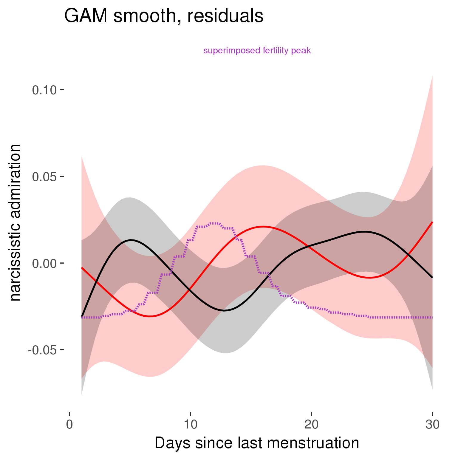
GAM smooth on raw data
As before, but without partialling anything out.
tryCatch({
trend_plot = ggplot(tmp,aes_string(x = "RCD", y = outcome, colour = "included")) +
stat_smooth(geom = 'smooth',size = 0.8, fill = "#9ECAE1", method = 'gam', formula = y ~ s(x))
}, error = function(e){cat_message(e, "danger")})
tryCatch({
trend_data = ggplot_build(trend_plot)$data[[1]]
}, error = function(e){cat_message(e, "danger")})
trend_data$RCD = round(trend_data$x)
trend_data = left_join(trend_data, tmp %>% select(real, RCD,fertile) %>% unique(), by = "RCD")
trend_data %>%
filter(real == TRUE) %>%
mutate(superimposed = ( ( (fertile - 0.01)/0.58) * (max(y)-min(y) ) ) + min(y) ) ->
trend_data
plot1b = ggplot(trend_data) +
geom_ribbon(aes(x = x, ymin = ymin, ymax = ymax, fill = factor(group)), alpha = 0.2) +
geom_line(aes(x = x, y = y, colour = factor(group)), size = 0.8, stat = "identity") +
scale_x_continuous(caption_x) +
geom_line(aes(x = x, y = superimposed), color = "#a83fbf", size = 1, linetype = 'dashed') +
annotate("text",x = mean(trend_data$x), y = max(trend_data$superimposed,na.rm=T) + 0.1, label = 'superimposed fertility peak', color = "#a83fbf") +
scale_y_continuous(outcome_label) +
ggtitle("GAM smooth, raw data") +
scale_color_manual("Contraception status",values = c("2"="black","1"= "red"), labels = c("2"="hormonally\ncontracepting","1"="cycling"), guide = F) +
scale_fill_manual("Contraception status",values = c("2"="black","1"= "red"), labels = c("2"="hormonally\ncontracepting","1"="cycling"), guide = F)
suppressWarnings(print(plot1b))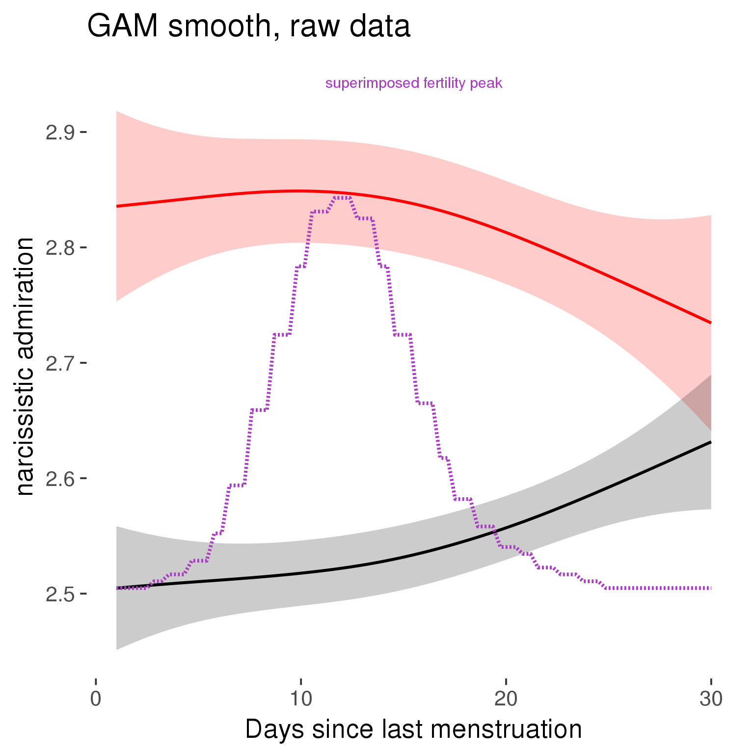
Means and standard errors over raw data
Nothing partialled out, just straight means with bootstrapped confidence intervals.
tryCatch({
trend_plot = ggplot(tmp,aes_string(x = "RCD", y = outcome, colour = "included")) +
geom_pointrange(size = 0.8, stat = 'summary', fun.data = "mean_cl_boot")
}, error = function(e){cat_message(e, "danger")})
tryCatch({
trend_data = ggplot_build(trend_plot)$data[[1]]
}, error = function(e){cat_message(e, "danger")})
trend_data$RCD = round(trend_data$x)
trend_data = left_join(trend_data, tmp %>% select(real, RCD,fertile) %>% unique(), by = "RCD")
trend_data %>%
filter(real == TRUE) %>%
mutate(superimposed = ( ( (fertile - 0.01)/0.58) * (max(y)-min(y) ) ) + min(y) ) ->
trend_data
plot3 = ggplot(trend_data) +
geom_pointrange(aes(x = x, y = y, ymin = ymin,ymax = ymax, colour = factor(group)), size = 0.8, stat = "identity", alpha = 0.6, position = position_dodge(width = .5)) +
scale_x_continuous("Days until next menstruation") +
geom_line(aes(x= x, y = superimposed), color = "#a83fbf", size = 1, linetype = 'dashed') +
annotate("text",x = mean(trend_data$x), y = max(trend_data$superimposed,na.rm=T) + 0.1, label = 'superimposed fertility peak', color = "#a83fbf") +
scale_y_continuous(outcome_label) +
ggtitle("Means with standard errors, raw data") +
scale_color_manual("Contraception status",values = c("2"="black","1"= "red"), labels = c("2"="hormonally\ncontracepting","1"="cycling"), guide = F) +
scale_fill_manual("Contraception status",values = c("2"="black","1"= "red"), labels = c("2"="hormonally\ncontracepting","1"="cycling"), guide = F)
suppressWarnings(print(plot3))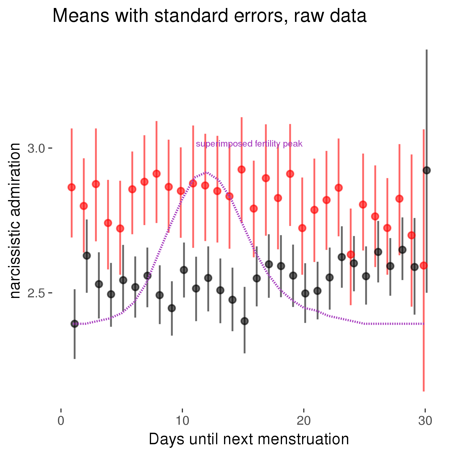
Robustness checks
M_r1: Random slopes for conception risk and menstruation
tryCatch({
# refit model with random effects for fertile and menstruation dummies
with_ind_diff = update(model, formula = . ~ . - (1| person) + (1 + fertile + menstruation | person))
# pull the random effects, format as tibble
rand = coef(with_ind_diff)$person %>%
tibble::rownames_to_column("person") %>%
mutate(person = as.numeric(person))
# pull the fixed effects
fixd = data.frame(fixef(with_ind_diff)) %>%
tibble::rownames_to_column("effect")
names(fixd) = c("effect", "pop_effect_size")
# pull apart the coefficients so that we can account for the fact that the random effect variation implicitly includes HC explaining the mean population-level effect of fertile/menstruation dummies among HC users
fixd = fixd %>%
separate(effect, c("included", "effect"), sep = ":", fill = "left") %>%
mutate(included = if_else(is.na(included), "cycling", str_replace(included, "included", "")))
fixd[2,c("included", "effect")] = c("horm_contra", "(Intercept)")
rand = rand %>%
# merge diary data on the random effects, so that we know who is a HC users and who isn't
inner_join(diary %>% select(person, included) %>% unique(), by = 'person') %>%
# gather into long format, to have the dataset by predictor
gather(effect, value, -person, -included) %>%
inner_join(fixd, by = c('effect', 'included')) %>%
# pull the fixed effects
mutate(
# only for those who are HC users, add the moderated population effect size for this effect (the random effects have the reference category mean)
value = if_else(included == "horm_contra", value + pop_effect_size, value),
effect = recode(effect, "includedhorm_contra" = "HC user",
"includedhorm_contra:fertile" = "HC user x fertile",
"includedhorm_contra:menstruationpre" = "HC user x premens.",
"includedhorm_contra:menstruationyes" = "HC user x mens.",
"menstruationyes" = "mens.",
"menstruationpre" = "premens.")) %>%
group_by(included, effect) %>%
# filter out predictors that aren't modelled as varying/random
filter(sd(value) > 0)
# plot dot plot of random effects
print(
ggplot(rand, aes(x = included, y = value, color = included, fill = included)) +
facet_wrap( ~ effect, scales = "free") +
# geom_violin(alpha = 0.4, size = 0) +
geom_dotplot(binaxis='y', dotsize = 0.1, method = "histodot") +
# geom_jitter(alpha = 0.05) +
coord_flip() +
geom_pointrange(stat = 'summary', fun.data = 'mean_sdl', color = 'darkred', size = 1.2) +
scale_color_manual("Contraception status", values = c("horm_contra"="black","cycling"= "red"), labels = c("horm_contra"="hormonally\ncontracepting","cycling"="cycling"), guide = F) +
scale_fill_manual("Contraception status", values = c("horm_contra"="black","cycling"= "red"), labels = c("horm_contra"="hormonally\ncontracepting","1"="cycling"), guide = F) +
ggtitle("M_r1: allowing participant-varying slopes", subtitle = "for the conception risk measure and the menstruation dummies") +
scale_x_discrete("Hormonal contraception", breaks = c("horm_contra", "cycling"), labels = c("yes", "no")) +
scale_y_continuous("Random effect size distribution"))
print_summary(with_ind_diff)
cat(pander(anova(model, with_ind_diff)))
}, error = function(e){
with_ind_diff = model
cat_message(e, "danger")
})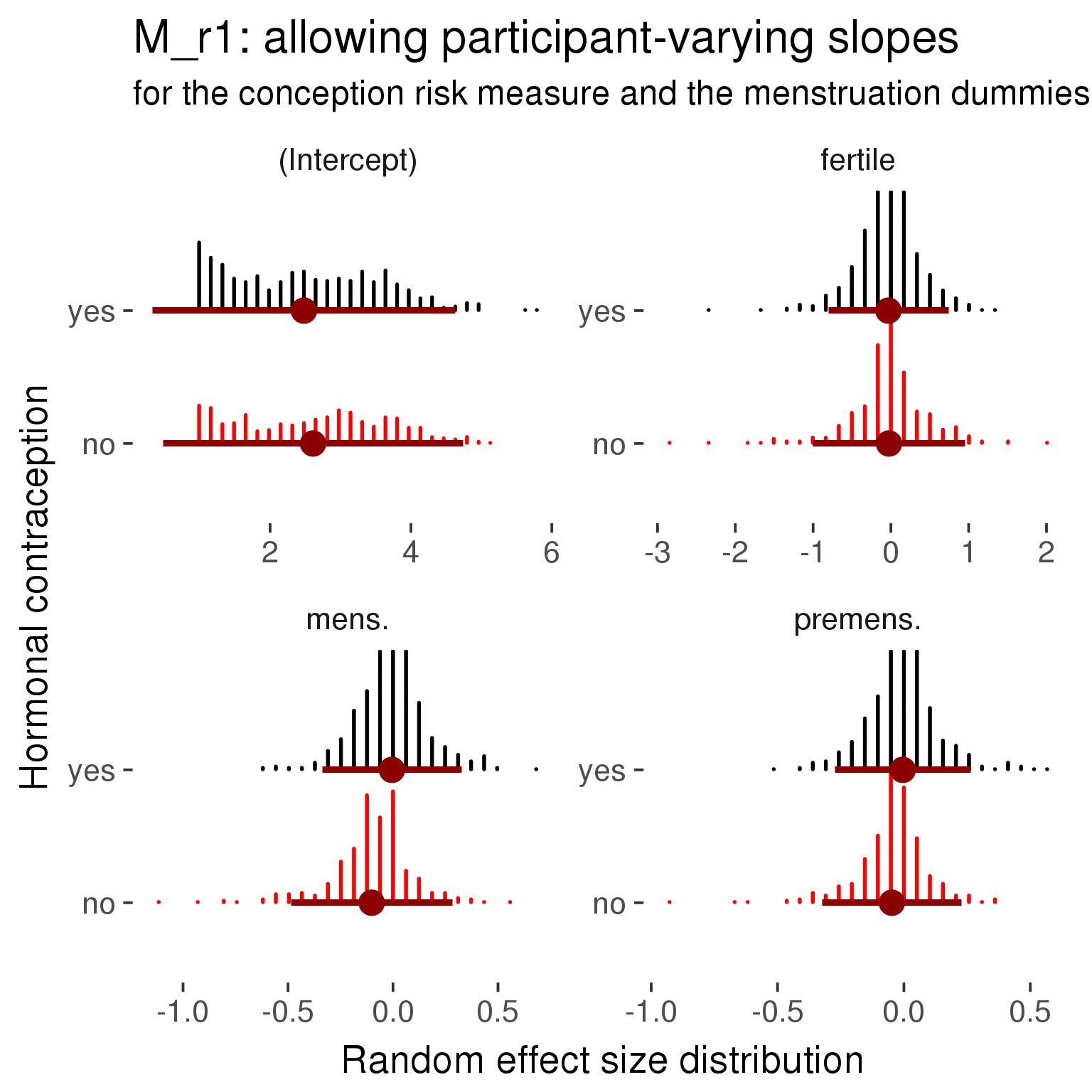
Linear mixed model fit by REML ['lmerMod']
Formula: NARQ_admiration ~ included + menstruation + fertile + fertile_mean +
(1 + fertile + menstruation | person) + included:menstruation + included:fertile
Data: diary
REML criterion at convergence: 62553
Scaled residuals:
Min 1Q Median 3Q Max
-4.891 -0.504 -0.066 0.512 6.058
Random effects:
Groups Name Variance Std.Dev. Corr
person (Intercept) 1.2250 1.107
fertile 0.5038 0.710 -0.19
menstruationpre 0.0687 0.262 -0.23 0.17
menstruationyes 0.0969 0.311 -0.28 0.26 0.59
Residual 0.5009 0.708
Number of obs: 26682, groups: person, 1054
Fixed effects:
Estimate Std. Error t value
(Intercept) 2.6096 0.0866 30.13
includedhorm_contra -0.1290 0.0729 -1.77
menstruationpre -0.0476 0.0267 -1.79
menstruationyes -0.1016 0.0272 -3.74
fertile -0.0247 0.0599 -0.41
fertile_mean 0.2672 0.3866 0.69
includedhorm_contra:menstruationpre 0.0430 0.0342 1.26
includedhorm_contra:menstruationyes 0.0965 0.0354 2.73
includedhorm_contra:fertile -0.0073 0.0762 -0.10
Correlation of Fixed Effects:
(Intr) incld_ mnstrtnp mnstrtny fertil frtl_m inclddhrm_cntr:mnstrtnp
inclddhrm_c -0.487
menstrutnpr -0.160 0.189
menstrutnys -0.186 0.218 0.457
fertile -0.135 0.209 0.350 0.331
fertile_men -0.760 -0.021 0.001 0.004 -0.053
inclddhrm_cntr:mnstrtnp 0.128 -0.241 -0.779 -0.356 -0.272 -0.005
inclddhrm_cntr:mnstrtny 0.145 -0.275 -0.351 -0.768 -0.254 -0.006 0.447
inclddhrm_cntr:f 0.130 -0.266 -0.275 -0.260 -0.784 0.009 0.349
inclddhrm_cntr:mnstrtny
inclddhrm_c
menstrutnpr
menstrutnys
fertile
fertile_men
inclddhrm_cntr:mnstrtnp
inclddhrm_cntr:mnstrtny
inclddhrm_cntr:f 0.327
refitting model(s) with ML (instead of REML)
| Df | AIC | BIC | logLik | deviance | Chisq | Chi Df | Pr(>Chisq) | |
|---|---|---|---|---|---|---|---|---|
| object | 11 | 62998 | 63088 | -31488 | 62976 | NA | NA | NA |
| ..1 | 20 | 62554 | 62717 | -31257 | 62514 | 462.2 | 9 | 7.118e-94 |
robustness_check_ovu_shift(model, diary)M_e: Exclusion criteria
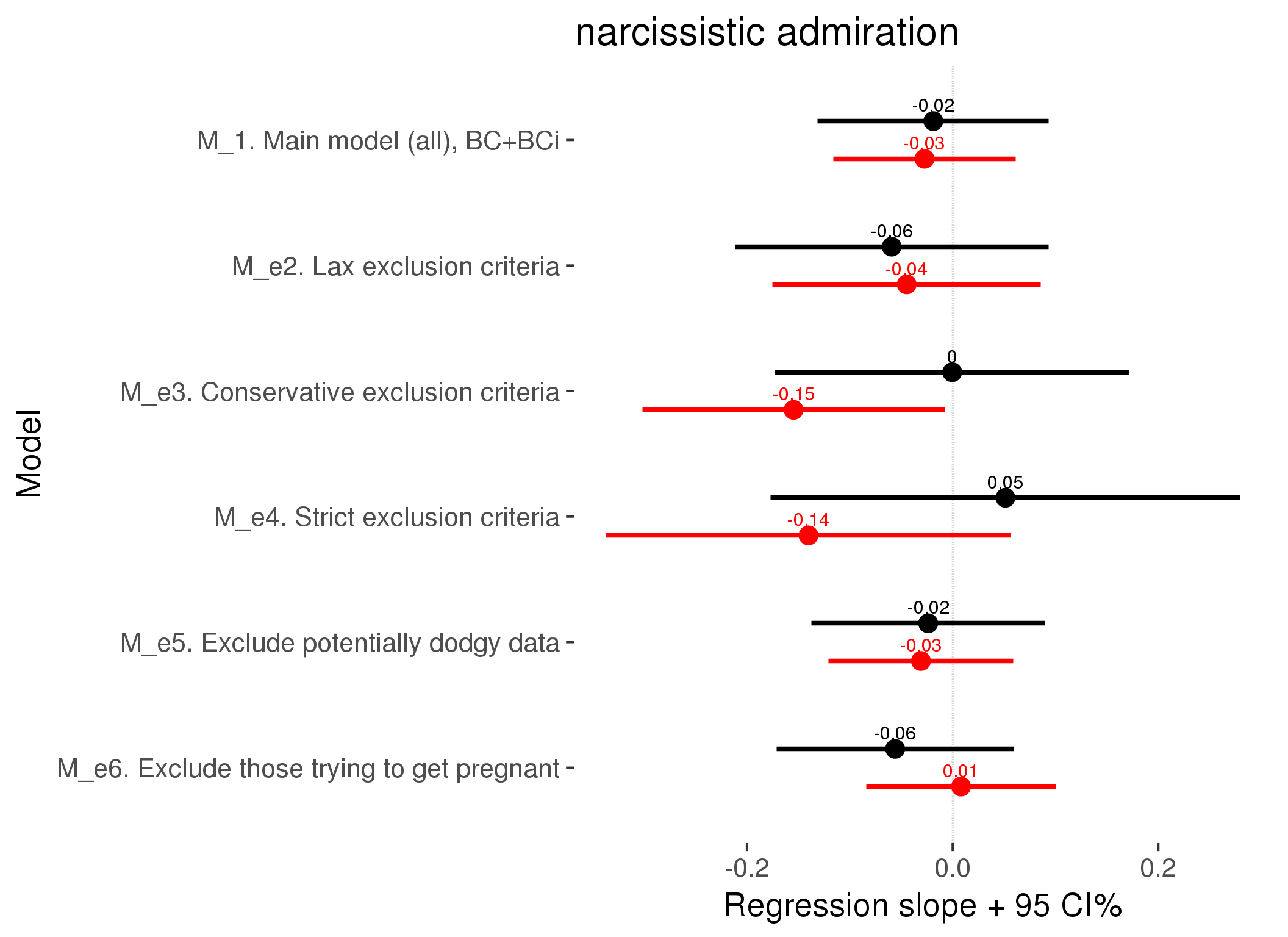
M_p: Predictors
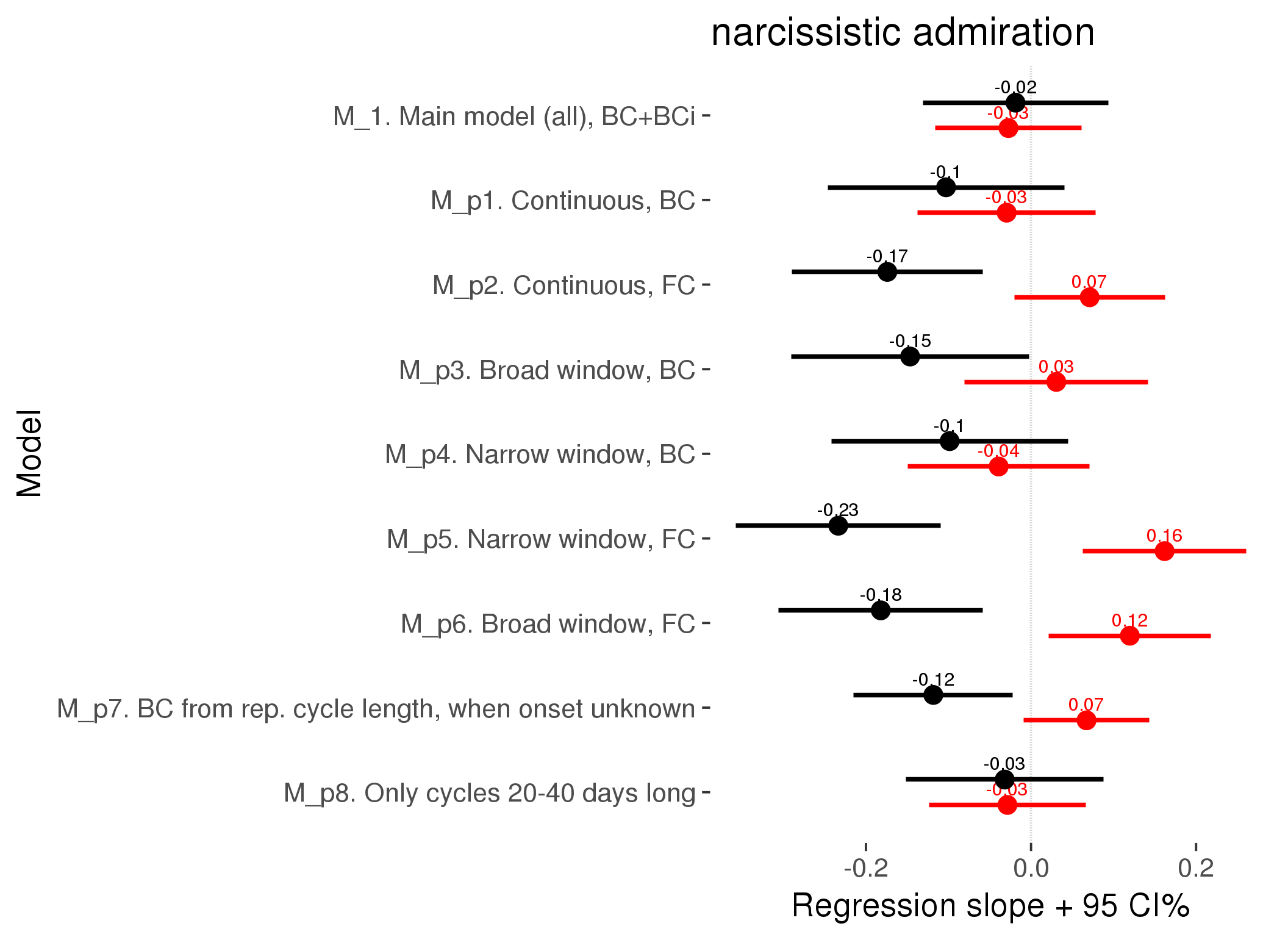
M_c: Covariates, controls, autocorrelation
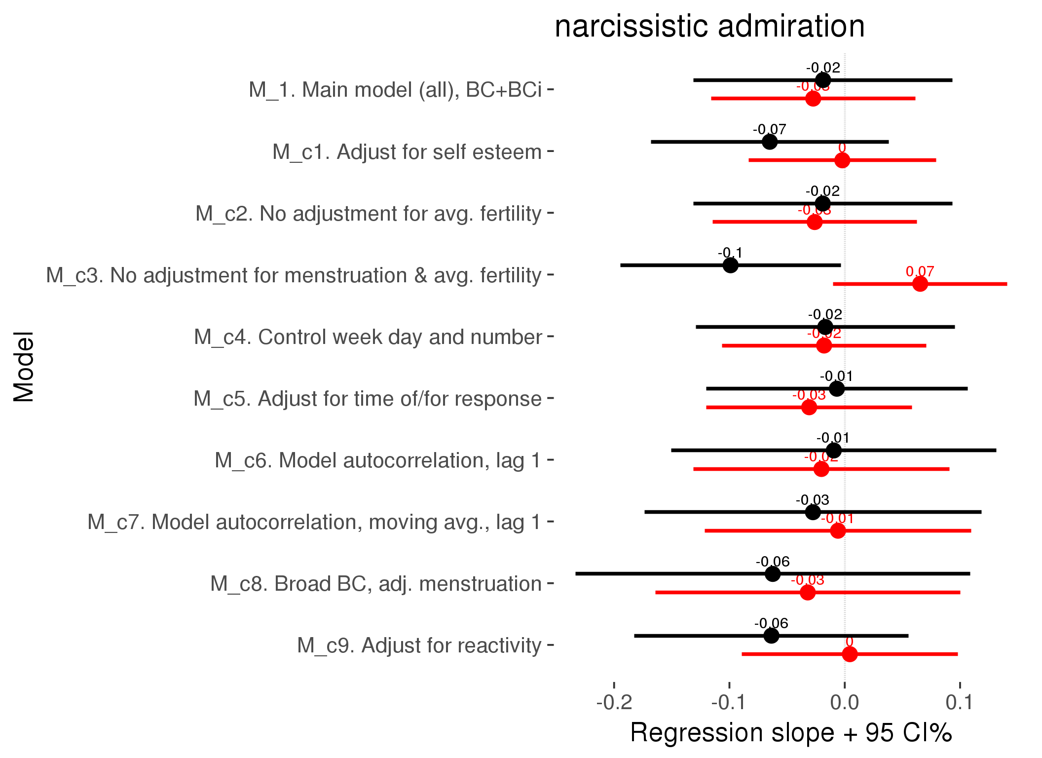
Linear mixed model fit by REML ['lmerMod']
REML criterion at convergence: 57426
Scaled residuals:
Min 1Q Median 3Q Max
-5.181 -0.514 -0.080 0.530 5.956
Random effects:
Groups Name Variance Std.Dev.
person (Intercept) 1.1215 1.059
Xr.2 s(days_filled_out):includedhorm_contra 0.0000 0.000
Xr.1 s(days_filled_out):includedcycling 0.0460 0.214
Xr.0 s(day_number):includedhorm_contra 0.0000 0.000
Xr s(day_number):includedcycling 0.0547 0.234
Residual 0.5260 0.725
Number of obs: 24379, groups: person, 1054; Xr.2, 8; Xr.1, 8; Xr.0, 8; Xr, 8
Fixed effects:
Estimate Std. Error t value
X(Intercept) 2.59283 0.08464 30.63
Xincludedhorm_contra -0.10245 0.07025 -1.46
Xmenstruationpre -0.04009 0.02324 -1.73
Xmenstruationyes -0.09238 0.02234 -4.14
Xfertile 0.00444 0.04787 0.09
Xfertile_mean 0.29186 0.38033 0.77
Xincludedhorm_contra:menstruationpre 0.02861 0.02978 0.96
Xincludedhorm_contra:menstruationyes 0.06763 0.02921 2.32
Xincludedhorm_contra:fertile -0.06357 0.06064 -1.05
Xs(day_number):includedcyclingFx1 0.09107 0.08419 1.08
Xs(day_number):includedhorm_contraFx1 -0.00243 0.03259 -0.07
Xs(days_filled_out):includedcyclingFx1 -0.10481 0.08339 -1.26
Xs(days_filled_out):includedhorm_contraFx1 0.03528 0.03346 1.05
Family: gaussian
Link function: identity
Formula:
NARQ_admiration ~ included + menstruation + fertile + fertile_mean +
s(day_number, by = included) + s(days_filled_out, by = included) +
included:menstruation + included:fertile
Parametric coefficients:
Estimate Std. Error t value Pr(>|t|)
(Intercept) 2.59283 0.08464 30.63 < 2e-16 ***
includedhorm_contra -0.10245 0.07025 -1.46 0.145
menstruationpre -0.04009 0.02324 -1.73 0.084 .
menstruationyes -0.09238 0.02234 -4.14 0.000036 ***
fertile 0.00444 0.04787 0.09 0.926
fertile_mean 0.29186 0.38033 0.77 0.443
includedhorm_contra:menstruationpre 0.02861 0.02978 0.96 0.337
includedhorm_contra:menstruationyes 0.06763 0.02921 2.32 0.021 *
includedhorm_contra:fertile -0.06357 0.06064 -1.05 0.294
---
Signif. codes: 0 '***' 0.001 '**' 0.01 '*' 0.05 '.' 0.1 ' ' 1
Approximate significance of smooth terms:
edf Ref.df F p-value
s(day_number):includedcycling 3.67 3.67 1.19 0.25
s(day_number):includedhorm_contra 1.00 1.00 0.01 0.94
s(days_filled_out):includedcycling 3.43 3.43 1.66 0.16
s(days_filled_out):includedhorm_contra 1.00 1.00 1.11 0.29
R-sq.(adj) = 0.00208
lmer.REML = 57427 Scale est. = 0.52602 n = 24379
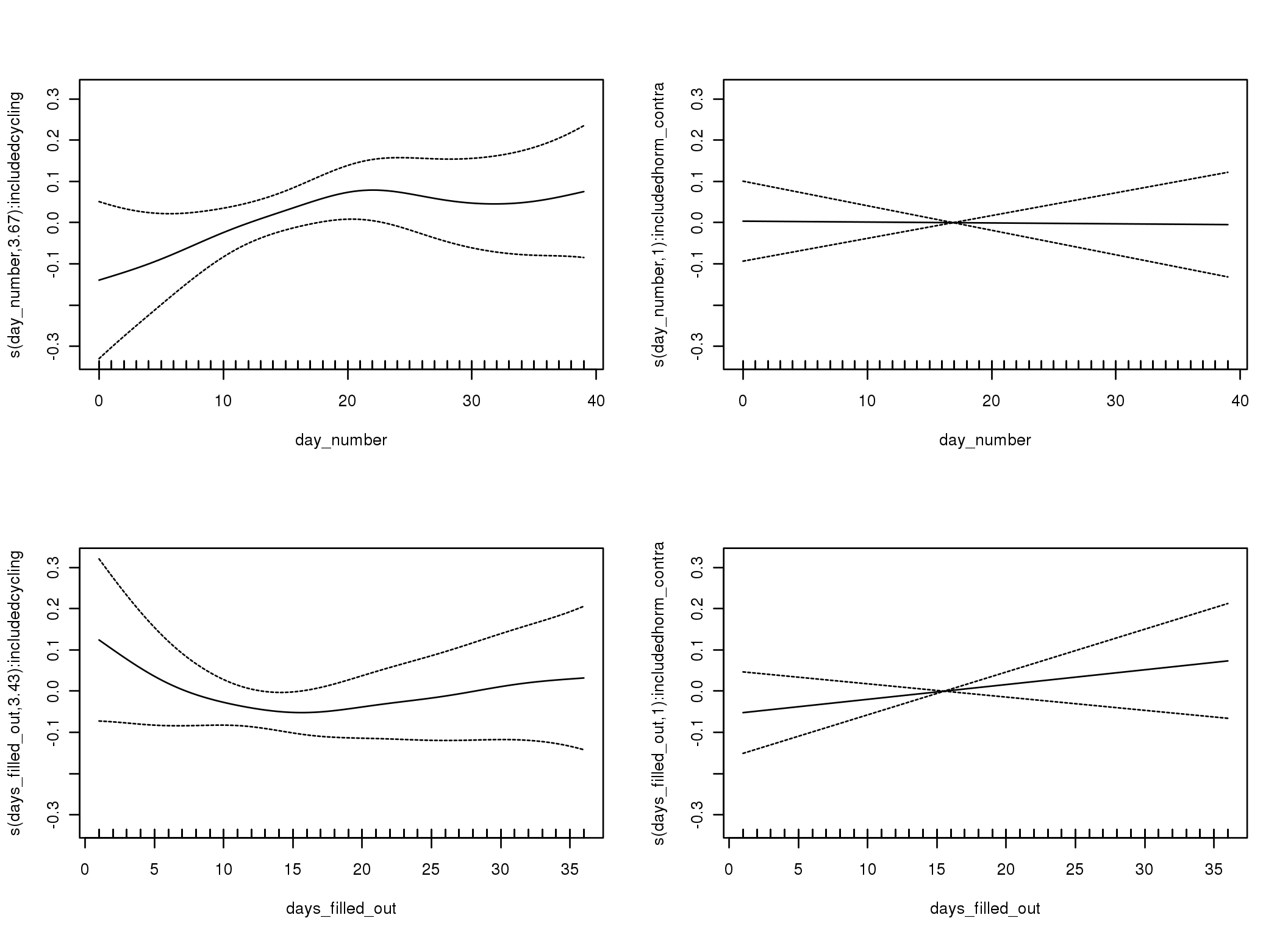
Linear mixed-effects model fit by REML
Data: diary
AIC BIC logLik
60976 61075 -30476
Random effects:
Formula: ~1 | person
(Intercept) Residual
StdDev: 1.06 0.7454
Correlation Structure: ARMA(1,0)
Formula: ~day_number | person
Parameter estimate(s):
Phi1
0.3344
Fixed effects: NARQ_admiration ~ included * (menstruation + fertile) + fertile_mean
Value Std.Error DF t-value p-value
(Intercept) 2.6217 0.0859 25622 30.526 0.0000
includedhorm_contra -0.1252 0.0712 1051 -1.760 0.0787
menstruationpre -0.0372 0.0263 25622 -1.414 0.1574
menstruationyes -0.0929 0.0246 25622 -3.778 0.0002
fertile -0.0202 0.0567 25622 -0.357 0.7213
fertile_mean 0.2019 0.3873 1051 0.521 0.6023
includedhorm_contra:menstruationpre 0.0358 0.0338 25622 1.057 0.2905
includedhorm_contra:menstruationyes 0.0845 0.0320 25622 2.641 0.0083
includedhorm_contra:fertile -0.0095 0.0718 25622 -0.132 0.8947
Correlation:
(Intr) incld_ mnstrtnp mnstrtny fertil frtl_m inclddhrm_cntr:mnstrtnp
includedhorm_contra -0.480
menstruationpre -0.113 0.144
menstruationyes -0.113 0.142 0.406
fertile -0.111 0.186 0.419 0.357
fertile_mean -0.768 -0.021 -0.007 -0.005 -0.055
includedhorm_contra:menstruationpre 0.094 -0.180 -0.779 -0.316 -0.326 -0.002
includedhorm_contra:menstruationyes 0.091 -0.173 -0.312 -0.768 -0.274 -0.001 0.391
includedhorm_contra:fertile 0.113 -0.235 -0.331 -0.281 -0.788 0.011 0.418
inclddhrm_cntr:mnstrtny
includedhorm_contra
menstruationpre
menstruationyes
fertile
fertile_mean
includedhorm_contra:menstruationpre
includedhorm_contra:menstruationyes
includedhorm_contra:fertile 0.350
Standardized Within-Group Residuals:
Min Q1 Med Q3 Max
-5.08436 -0.51756 -0.08794 0.51760 5.78743
Number of Observations: 26682
Number of Groups: 1054
Linear mixed-effects model fit by REML
Data: diary
AIC BIC logLik
60309 60415 -30141
Random effects:
Formula: ~1 | person
(Intercept) Residual
StdDev: 1.028 0.7799
Correlation Structure: ARMA(1,1)
Formula: ~day_number | person
Parameter estimate(s):
Phi1 Theta1
0.8540 -0.6009
Fixed effects: NARQ_admiration ~ included * (menstruation + fertile) + fertile_mean
Value Std.Error DF t-value p-value
(Intercept) 2.6159 0.0856 25622 30.565 0.0000
includedhorm_contra -0.1201 0.0707 1051 -1.699 0.0896
menstruationpre -0.0285 0.0256 25622 -1.113 0.2659
menstruationyes -0.0794 0.0247 25622 -3.220 0.0013
fertile -0.0058 0.0590 25622 -0.099 0.9211
fertile_mean 0.2024 0.3873 1051 0.523 0.6013
includedhorm_contra:menstruationpre 0.0308 0.0329 25622 0.935 0.3497
includedhorm_contra:menstruationyes 0.0755 0.0319 25622 2.364 0.0181
includedhorm_contra:fertile -0.0276 0.0745 25622 -0.370 0.7115
Correlation:
(Intr) incld_ mnstrtnp mnstrtny fertil frtl_m inclddhrm_cntr:mnstrtnp
includedhorm_contra -0.477
menstruationpre -0.108 0.132
menstruationyes -0.114 0.141 0.453
fertile -0.104 0.183 0.315 0.325
fertile_mean -0.769 -0.022 -0.002 -0.004 -0.060
includedhorm_contra:menstruationpre 0.086 -0.164 -0.777 -0.352 -0.245 -0.002
includedhorm_contra:menstruationyes 0.091 -0.173 -0.350 -0.772 -0.251 -0.001 0.443
includedhorm_contra:fertile 0.110 -0.231 -0.250 -0.257 -0.790 0.012 0.314
inclddhrm_cntr:mnstrtny
includedhorm_contra
menstruationpre
menstruationyes
fertile
fertile_mean
includedhorm_contra:menstruationpre
includedhorm_contra:menstruationyes
includedhorm_contra:fertile 0.320
Standardized Within-Group Residuals:
Min Q1 Med Q3 Max
-4.7192 -0.5138 -0.1346 0.5285 5.4535
Number of Observations: 26682
Number of Groups: 1054
M_d: Other designs
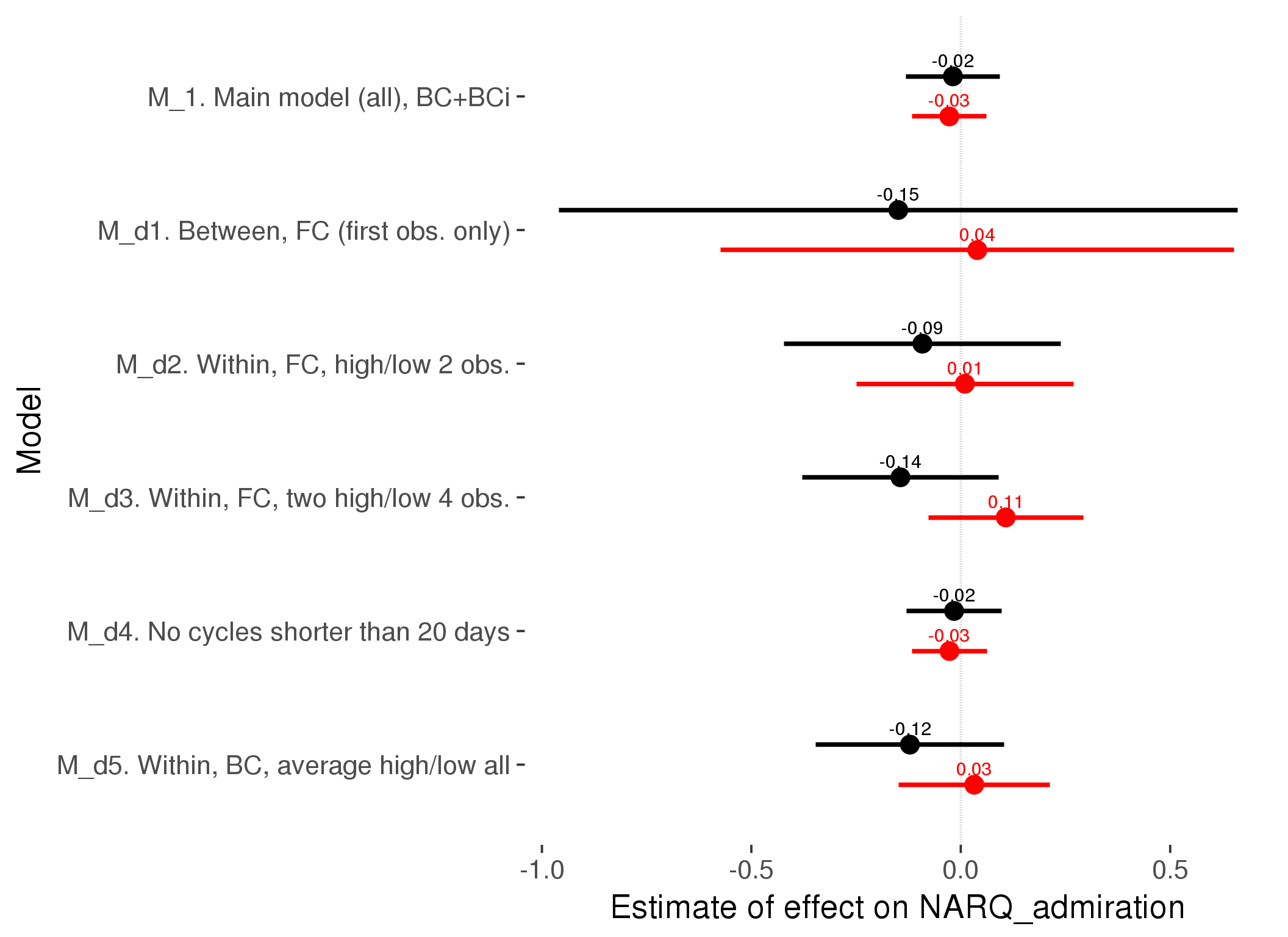
M_m1: Moderation by contraceptive method
Based on the sample with lax exclusion criteria. Users who used any hormonal contraception are classified as hormonal, users who use any awareness-based methods (counting, temperature-based) are classified as ‘fertility-awareness’, women who don’t fall into the before groups and use condoms, pessars, coitus interruptus etc. are classified as ‘barrie or abstinence’. Women who don’t use contraception or use other methods such as sterilisation are excluded from this analysis.
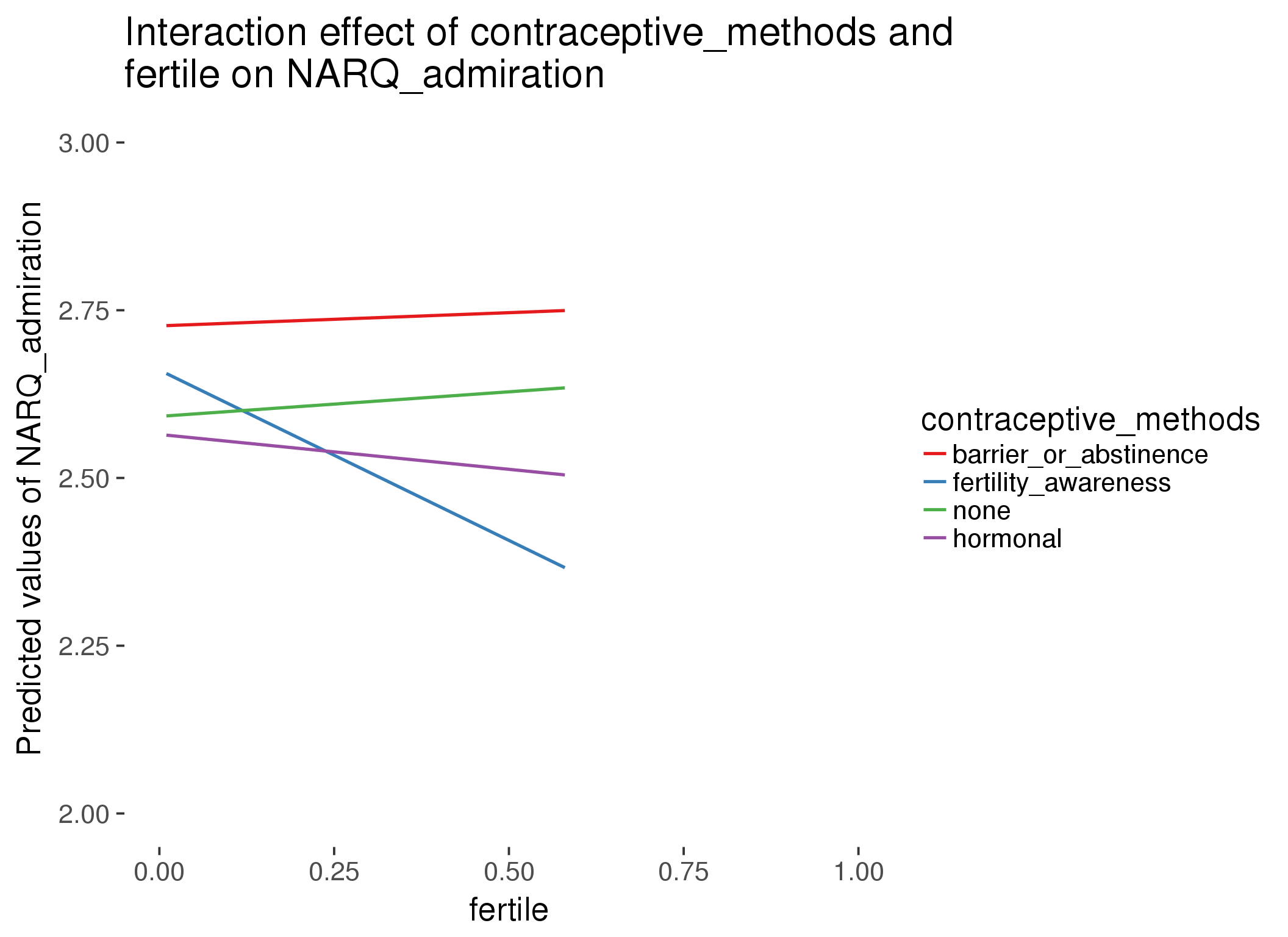
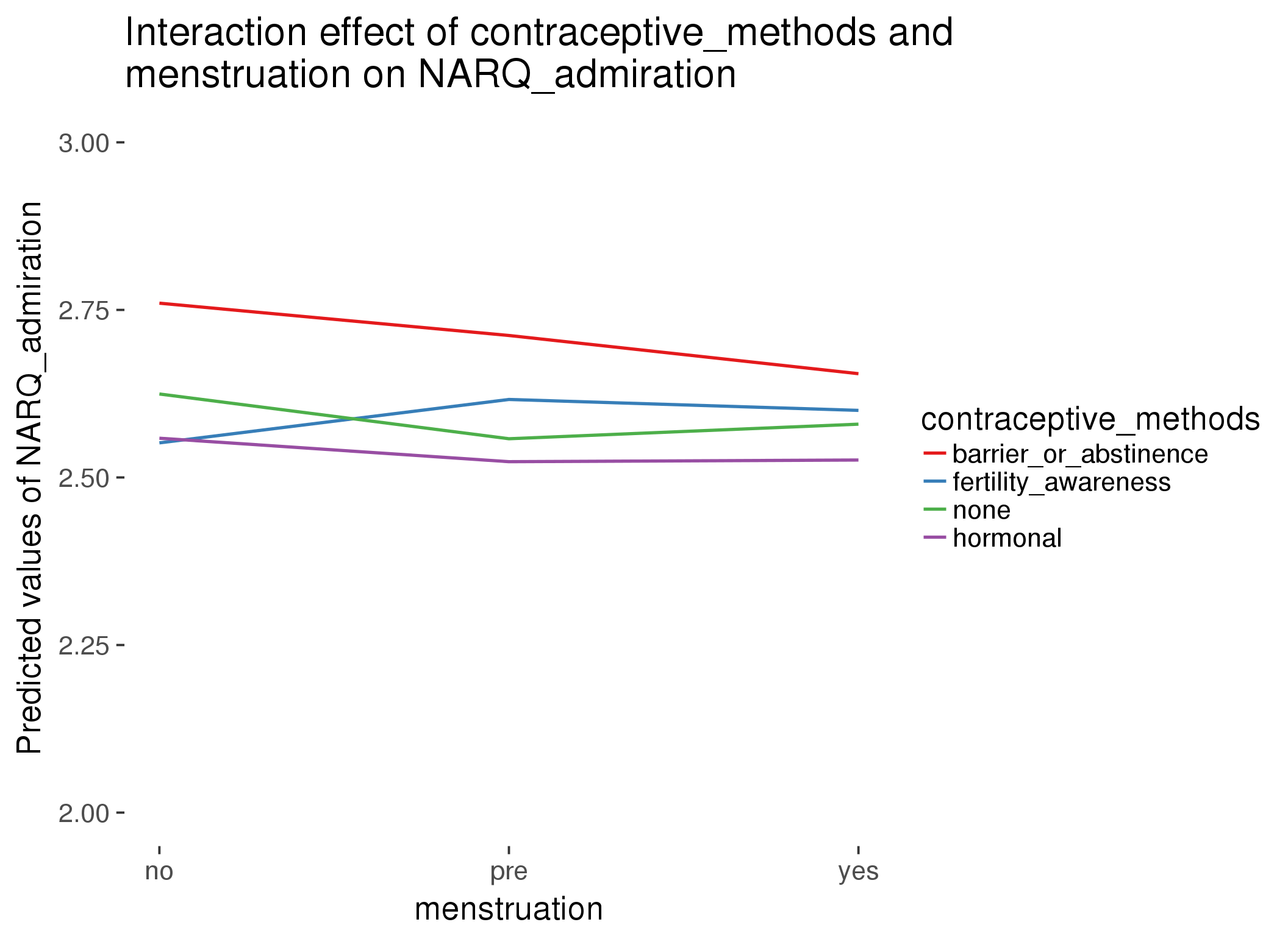
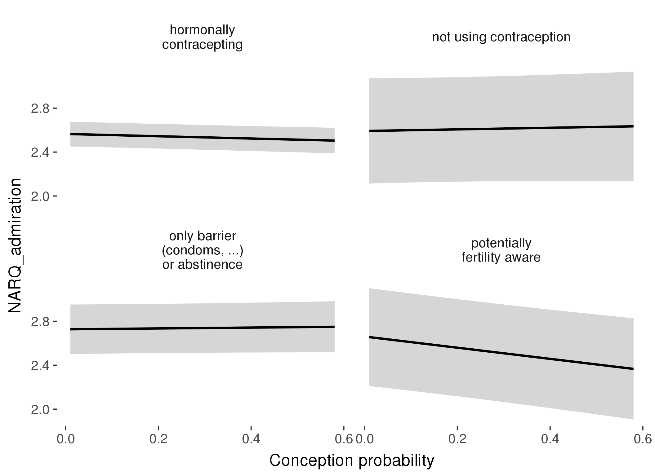
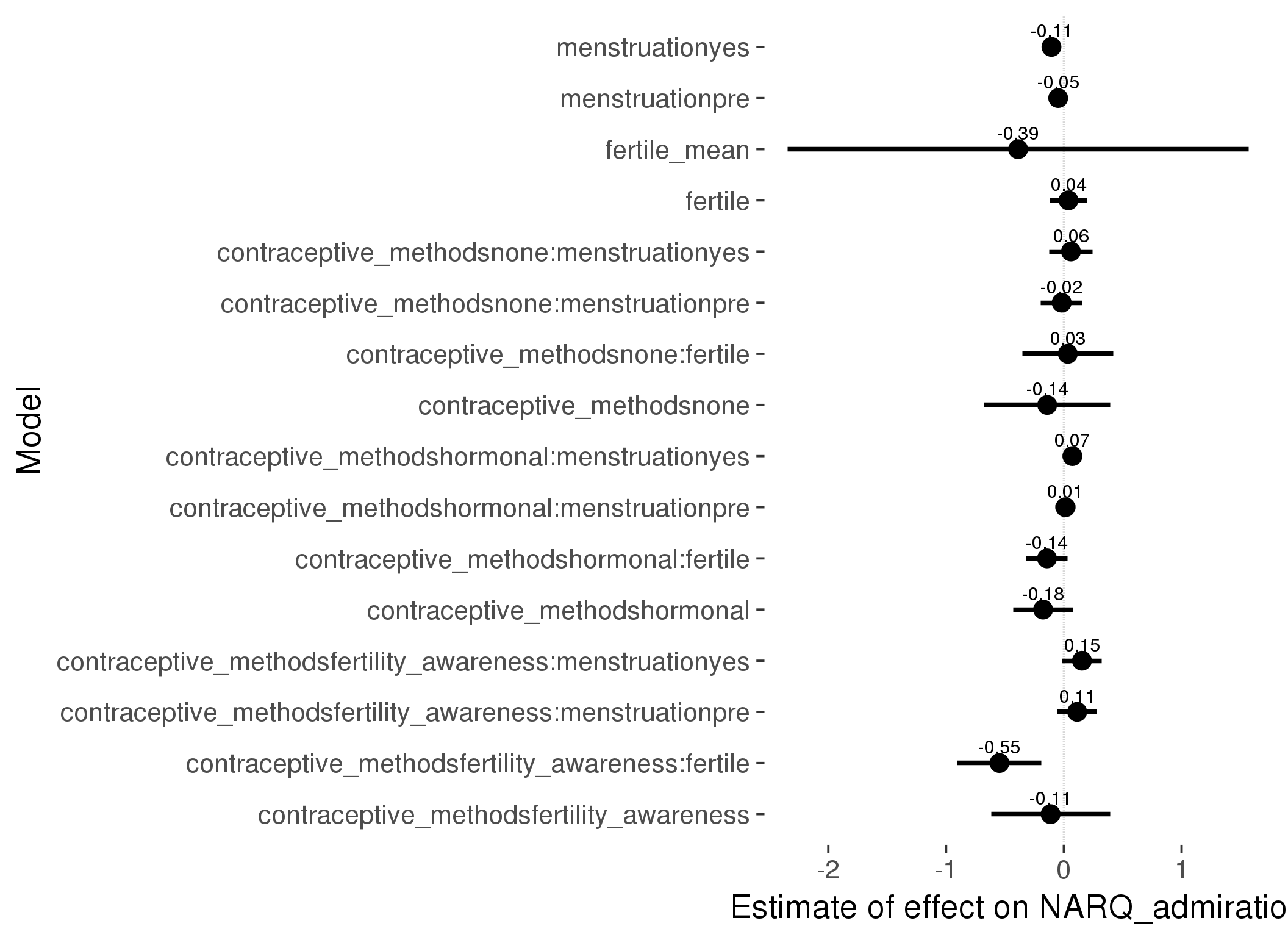
Linear mixed model fit by REML ['lmerMod']
Formula: NARQ_admiration ~ fertile_mean + (1 | person) + contraceptive_methods +
fertile + menstruation + fertile:contraceptive_methods + menstruation:contraceptive_methods
Data: diary
Subset: !is.na(included_lax) & contraceptive_method != "other"
REML criterion at convergence: 39370
Scaled residuals:
Min 1Q Median 3Q Max
-5.311 -0.509 -0.074 0.534 4.835
Random effects:
Groups Name Variance Std.Dev.
person (Intercept) 1.204 1.097
Residual 0.518 0.719
Number of obs: 17028, groups: person, 513
Fixed effects:
Estimate Std. Error t value
(Intercept) 2.8212 0.2039 13.83
fertile_mean -0.3883 0.9992 -0.39
contraceptive_methodsfertility_awareness -0.1124 0.2579 -0.44
contraceptive_methodsnone -0.1415 0.2728 -0.52
contraceptive_methodshormonal -0.1763 0.1303 -1.35
fertile 0.0394 0.0804 0.49
menstruationpre -0.0482 0.0388 -1.24
menstruationyes -0.1052 0.0371 -2.84
contraceptive_methodsfertility_awareness:fertile -0.5471 0.1824 -3.00
contraceptive_methodsnone:fertile 0.0339 0.1975 0.17
contraceptive_methodshormonal:fertile -0.1433 0.0898 -1.60
contraceptive_methodsfertility_awareness:menstruationpre 0.1129 0.0859 1.31
contraceptive_methodsnone:menstruationpre -0.0185 0.0899 -0.21
contraceptive_methodshormonal:menstruationpre 0.0132 0.0437 0.30
contraceptive_methodsfertility_awareness:menstruationyes 0.1536 0.0864 1.78
contraceptive_methodsnone:menstruationyes 0.0602 0.0939 0.64
contraceptive_methodshormonal:menstruationyes 0.0727 0.0423 1.72
refitting model(s) with ML (instead of REML)
| Df | AIC | BIC | logLik | deviance | Chisq | Chi Df | Pr(>Chisq) | |
|---|---|---|---|---|---|---|---|---|
| add_main | 13 | 39371 | 39471 | -19672 | 39345 | NA | NA | NA |
| by_method | 19 | 39354 | 39501 | -19658 | 39316 | 29 | 6 | 0.0000609 |
M_m2: Moderation by participant age
model %>%
test_moderator("age_group", diary, xlevels = 5)refitting model(s) with ML (instead of REML)
| Df | AIC | BIC | logLik | deviance | Chisq | Chi Df | Pr(>Chisq) | |
|---|---|---|---|---|---|---|---|---|
| with_main | 19 | 63002 | 63158 | -31482 | 62964 | NA | NA | NA |
| with_mod | 27 | 63006 | 63227 | -31476 | 62952 | 12.15 | 8 | 0.1448 |
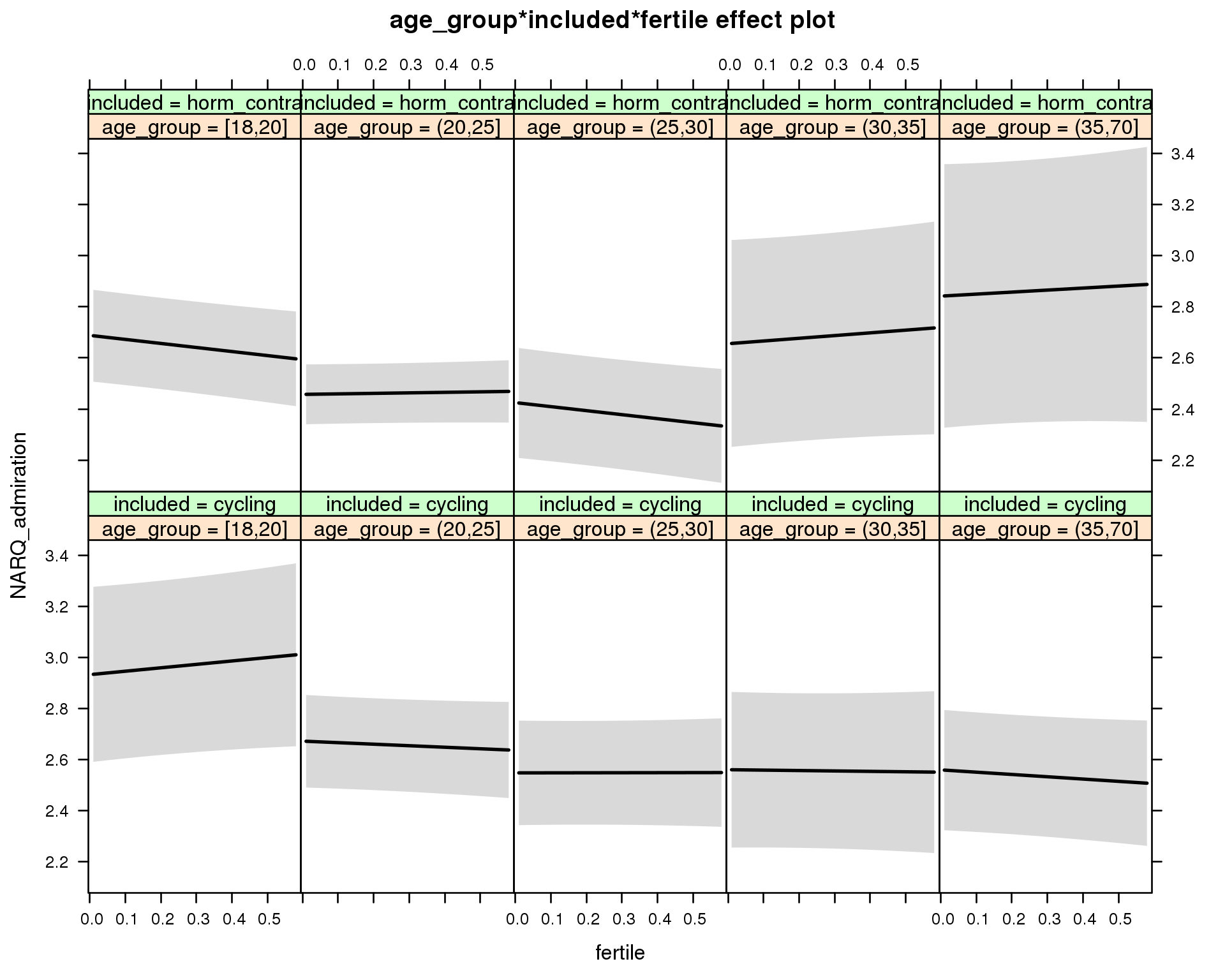
Linear mixed model fit by REML ['lmerMod']
Formula: NARQ_admiration ~ menstruation + fertile_mean + (1 | person) +
age_group + included + fertile + menstruation:included +
age_group:included + age_group:fertile + included:fertile + age_group:included:fertile
Data: diary
REML criterion at convergence: 63029
Scaled residuals:
Min 1Q Median 3Q Max
-5.222 -0.515 -0.074 0.531 5.936
Random effects:
Groups Name Variance Std.Dev.
person (Intercept) 1.136 1.066
Residual 0.535 0.732
Number of obs: 26682, groups: person, 1054
Fixed effects:
Estimate Std. Error t value
(Intercept) 2.9079 0.1831 15.88
menstruationpre -0.0479 0.0224 -2.14
menstruationyes -0.0988 0.0211 -4.68
fertile_mean 0.2889 0.3843 0.75
age_group(20,25] -0.2600 0.1978 -1.31
age_group(25,30] -0.3842 0.2035 -1.89
age_group(30,35] -0.3718 0.2338 -1.59
age_group(35,70] -0.3725 0.2117 -1.76
includedhorm_contra -0.2652 0.1978 -1.34
fertile 0.1337 0.1292 1.04
menstruationpre:includedhorm_contra 0.0384 0.0288 1.34
menstruationyes:includedhorm_contra 0.0810 0.0277 2.93
age_group(20,25]:includedhorm_contra 0.0292 0.2261 0.13
age_group(25,30]:includedhorm_contra 0.1212 0.2487 0.49
age_group(30,35]:includedhorm_contra 0.3392 0.3250 1.04
age_group(35,70]:includedhorm_contra 0.5260 0.3501 1.50
age_group(20,25]:fertile -0.1935 0.1431 -1.35
age_group(25,30]:fertile -0.1316 0.1475 -0.89
age_group(30,35]:fertile -0.1500 0.1709 -0.88
age_group(35,70]:fertile -0.2234 0.1542 -1.45
includedhorm_contra:fertile -0.2920 0.1433 -2.04
age_group(20,25]:includedhorm_contra:fertile 0.3718 0.1603 2.32
age_group(25,30]:includedhorm_contra:fertile 0.1327 0.1777 0.75
age_group(30,35]:includedhorm_contra:fertile 0.4144 0.2295 1.81
age_group(35,70]:includedhorm_contra:fertile 0.4605 0.2605 1.77
M_m3: Moderation by weekend
model %>%
test_moderator("weekend", diary, xlevels = 2) refitting model(s) with ML (instead of REML)
| Df | AIC | BIC | logLik | deviance | Chisq | Chi Df | Pr(>Chisq) | |
|---|---|---|---|---|---|---|---|---|
| with_main | 13 | 62978 | 63084 | -31476 | 62952 | NA | NA | NA |
| with_mod | 15 | 62981 | 63104 | -31475 | 62951 | 1.014 | 2 | 0.6022 |
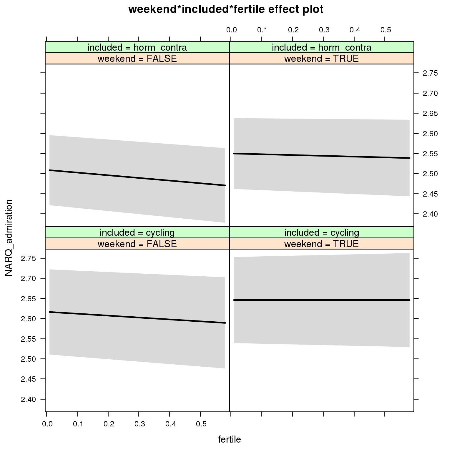
Linear mixed model fit by REML ['lmerMod']
Formula: NARQ_admiration ~ menstruation + fertile_mean + (1 | person) +
weekend + included + fertile + menstruation:included + weekend:included +
weekend:fertile + included:fertile + weekend:included:fertile
Data: diary
REML criterion at convergence: 63014
Scaled residuals:
Min 1Q Median 3Q Max
-5.250 -0.515 -0.075 0.531 5.980
Random effects:
Groups Name Variance Std.Dev.
person (Intercept) 1.139 1.067
Residual 0.535 0.731
Number of obs: 26682, groups: person, 1054
Fixed effects:
Estimate Std. Error t value
(Intercept) 2.598448 0.085388 30.43
menstruationpre -0.048358 0.022386 -2.16
menstruationyes -0.099945 0.021116 -4.73
fertile_mean 0.256003 0.382972 0.67
weekendTRUE 0.029176 0.019478 1.50
includedhorm_contra -0.129286 0.071033 -1.82
fertile -0.047468 0.054930 -0.86
menstruationpre:includedhorm_contra 0.039064 0.028739 1.36
menstruationyes:includedhorm_contra 0.083365 0.027676 3.01
weekendTRUE:includedhorm_contra 0.011729 0.025069 0.47
weekendTRUE:fertile 0.047488 0.075551 0.63
includedhorm_contra:fertile -0.018855 0.069849 -0.27
weekendTRUE:includedhorm_contra:fertile -0.000787 0.096080 -0.01
M_m4: Moderation by weekday
model %>%
test_moderator("weekday", diary, xlevels = 7)refitting model(s) with ML (instead of REML)
| Df | AIC | BIC | logLik | deviance | Chisq | Chi Df | Pr(>Chisq) | |
|---|---|---|---|---|---|---|---|---|
| with_main | 23 | 62985 | 63173 | -31469 | 62939 | NA | NA | NA |
| with_mod | 35 | 63002 | 63289 | -31466 | 62932 | 6.576 | 12 | 0.8843 |
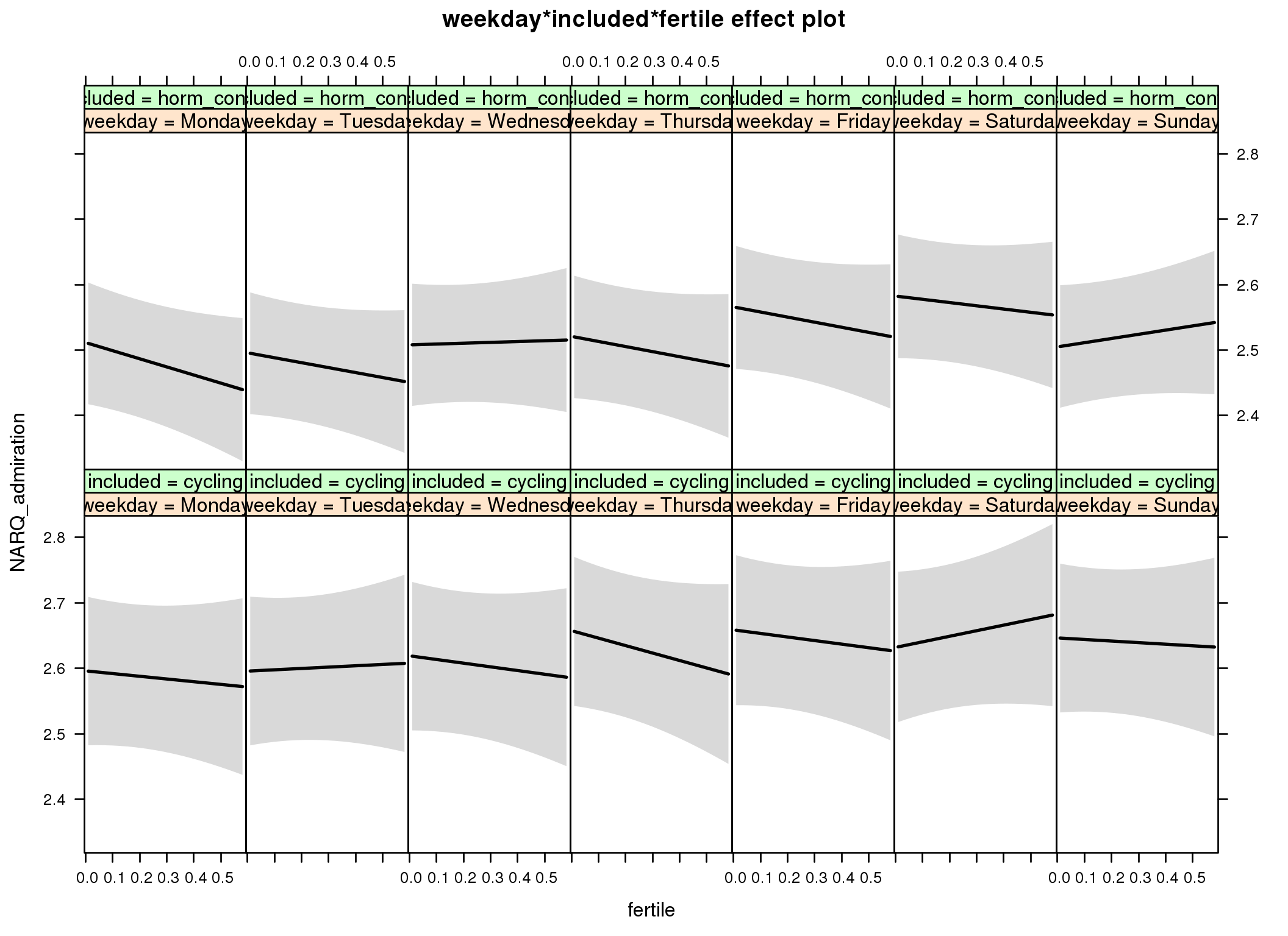
Linear mixed model fit by REML ['lmerMod']
Formula: NARQ_admiration ~ menstruation + fertile_mean + (1 | person) +
weekday + included + fertile + menstruation:included + weekday:included +
weekday:fertile + included:fertile + weekday:included:fertile
Data: diary
REML criterion at convergence: 63079
Scaled residuals:
Min 1Q Median 3Q Max
-5.250 -0.518 -0.074 0.533 5.982
Random effects:
Groups Name Variance Std.Dev.
person (Intercept) 1.140 1.067
Residual 0.535 0.731
Number of obs: 26682, groups: person, 1054
Fixed effects:
Estimate Std. Error t value
(Intercept) 2.577714 0.088021 29.29
menstruationpre -0.047812 0.022390 -2.14
menstruationyes -0.099537 0.021118 -4.71
fertile_mean 0.254386 0.383063 0.66
weekdayTuesday -0.000433 0.034844 -0.01
weekdayWednesday 0.022986 0.034789 0.66
weekdayThursday 0.061375 0.035184 1.74
weekdayFriday 0.062606 0.035779 1.75
weekdaySaturday 0.035797 0.036145 0.99
weekdaySunday 0.050339 0.034920 1.44
includedhorm_contra -0.105826 0.076072 -1.39
fertile -0.041401 0.098176 -0.42
menstruationpre:includedhorm_contra 0.038341 0.028743 1.33
menstruationyes:includedhorm_contra 0.082694 0.027680 2.99
weekdayTuesday:includedhorm_contra -0.015227 0.044763 -0.34
weekdayWednesday:includedhorm_contra -0.026540 0.044910 -0.59
weekdayThursday:includedhorm_contra -0.051953 0.045341 -1.15
weekdayFriday:includedhorm_contra -0.008171 0.045963 -0.18
weekdaySaturday:includedhorm_contra 0.035225 0.046500 0.76
weekdaySunday:includedhorm_contra -0.056951 0.045067 -1.26
weekdayTuesday:fertile 0.061880 0.135157 0.46
weekdayWednesday:fertile -0.014973 0.135762 -0.11
weekdayThursday:fertile -0.072633 0.137722 -0.53
weekdayFriday:fertile -0.013102 0.137920 -0.10
weekdaySaturday:fertile 0.126560 0.139754 0.91
weekdaySunday:fertile 0.017305 0.135845 0.13
includedhorm_contra:fertile -0.082599 0.125614 -0.66
weekdayTuesday:includedhorm_contra:fertile -0.013505 0.172483 -0.08
weekdayWednesday:includedhorm_contra:fertile 0.151704 0.173829 0.87
weekdayThursday:includedhorm_contra:fertile 0.118913 0.175233 0.68
weekdayFriday:includedhorm_contra:fertile 0.059320 0.175744 0.34
weekdaySaturday:includedhorm_contra:fertile -0.052192 0.178274 -0.29
weekdaySunday:includedhorm_contra:fertile 0.170766 0.173492 0.98
M_m5: Moderation by exclusion threshold
model %>%
test_moderator("included_levels", diary, xlevels = 4)refitting model(s) with ML (instead of REML)
| Df | AIC | BIC | logLik | deviance | Chisq | Chi Df | Pr(>Chisq) | |
|---|---|---|---|---|---|---|---|---|
| with_main | 17 | 63004 | 63143 | -31485 | 62970 | NA | NA | NA |
| with_mod | 23 | 62992 | 63181 | -31473 | 62946 | 23.25 | 6 | 0.0007182 |
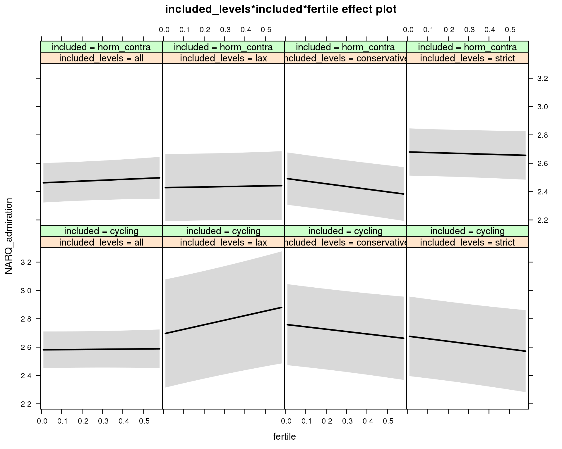
Linear mixed model fit by REML ['lmerMod']
Formula: NARQ_admiration ~ menstruation + fertile_mean + (1 | person) +
included_levels + included + fertile + menstruation:included +
included_levels:included + included_levels:fertile + included:fertile +
included_levels:included:fertile
Data: diary
REML criterion at convergence: 63019
Scaled residuals:
Min 1Q Median 3Q Max
-5.252 -0.516 -0.074 0.531 5.972
Random effects:
Groups Name Variance Std.Dev.
person (Intercept) 1.139 1.067
Residual 0.535 0.731
Number of obs: 26682, groups: person, 1054
Fixed effects:
Estimate Std. Error t value
(Intercept) 2.5673 0.0944 27.18
menstruationpre -0.0500 0.0224 -2.23
menstruationyes -0.1018 0.0211 -4.82
fertile_mean 0.2339 0.3849 0.61
included_levelslax 0.1122 0.2055 0.55
included_levelsconservative 0.1790 0.1601 1.12
included_levelsstrict 0.0967 0.1577 0.61
includedhorm_contra -0.1417 0.0978 -1.45
fertile 0.0127 0.0572 0.22
menstruationpre:includedhorm_contra 0.0388 0.0288 1.35
menstruationyes:includedhorm_contra 0.0819 0.0277 2.95
included_levelslax:includedhorm_contra -0.1460 0.2492 -0.59
included_levelsconservative:includedhorm_contra -0.1477 0.1989 -0.74
included_levelsstrict:includedhorm_contra 0.1213 0.1927 0.63
included_levelslax:fertile 0.3096 0.1393 2.22
included_levelsconservative:fertile -0.1807 0.1041 -1.74
included_levelsstrict:fertile -0.1958 0.1042 -1.88
includedhorm_contra:fertile 0.0486 0.0877 0.55
included_levelslax:includedhorm_contra:fertile -0.3465 0.1702 -2.04
included_levelsconservative:includedhorm_contra:fertile -0.0699 0.1356 -0.52
included_levelsstrict:includedhorm_contra:fertile 0.0931 0.1335 0.70
M_m6: Moderation by cycle length
model %>%
test_moderator("cycle_length_groups", diary, xlevels = 4)refitting model(s) with ML (instead of REML)
| Df | AIC | BIC | logLik | deviance | Chisq | Chi Df | Pr(>Chisq) | |
|---|---|---|---|---|---|---|---|---|
| with_main | 17 | 63004 | 63143 | -31485 | 62970 | NA | NA | NA |
| with_mod | 23 | 63010 | 63199 | -31482 | 62964 | 5.839 | 6 | 0.4414 |
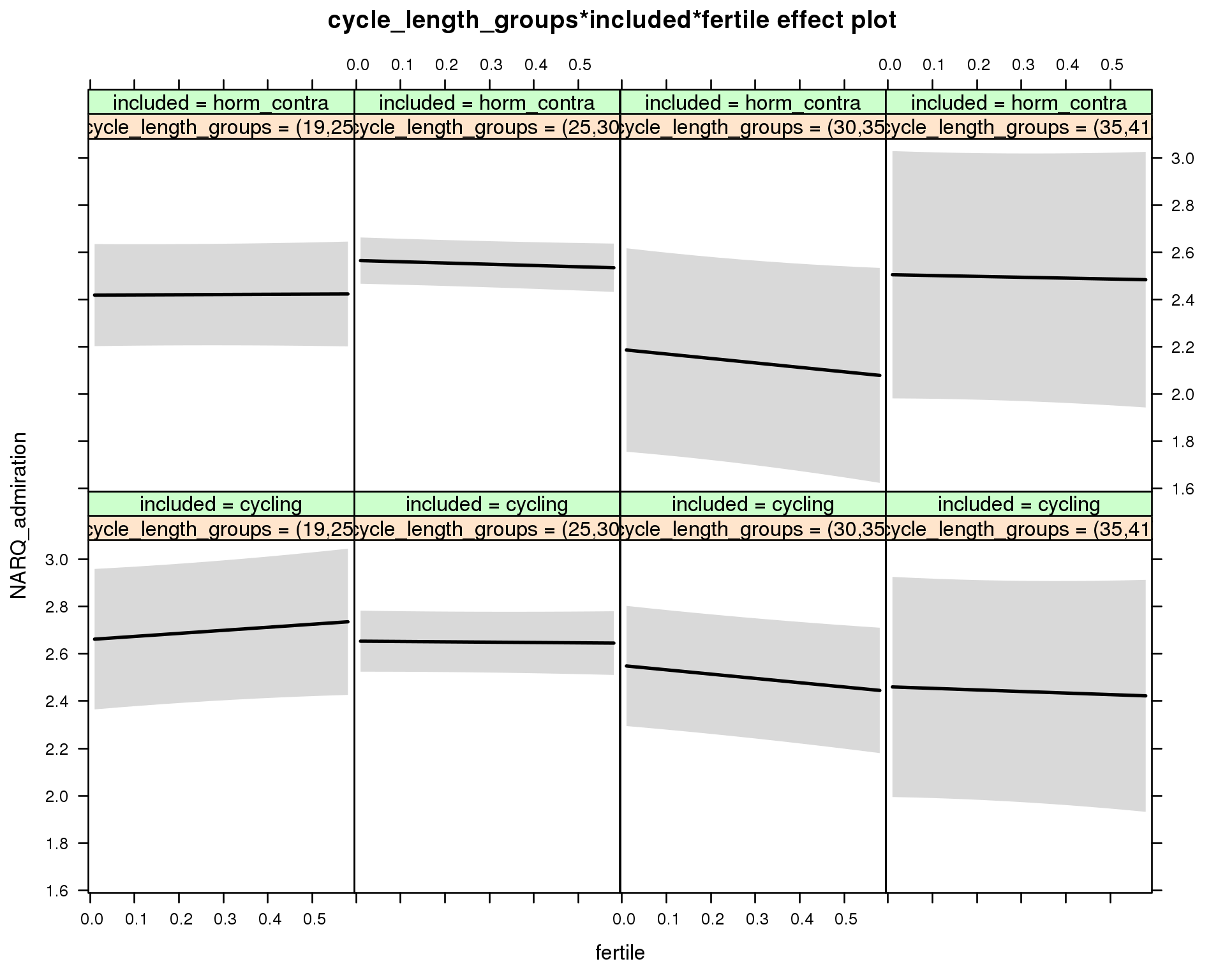
Linear mixed model fit by REML ['lmerMod']
Formula: NARQ_admiration ~ menstruation + fertile_mean + (1 | person) +
cycle_length_groups + included + fertile + menstruation:included +
cycle_length_groups:included + cycle_length_groups:fertile +
included:fertile + cycle_length_groups:included:fertile
Data: diary
REML criterion at convergence: 63029
Scaled residuals:
Min 1Q Median 3Q Max
-5.224 -0.517 -0.074 0.532 5.953
Random effects:
Groups Name Variance Std.Dev.
person (Intercept) 1.140 1.068
Residual 0.535 0.732
Number of obs: 26682, groups: person, 1054
Fixed effects:
Estimate Std. Error t value
(Intercept) 2.66083 0.16729 15.91
menstruationpre -0.04900 0.02243 -2.18
menstruationyes -0.10346 0.02128 -4.86
fertile_mean 0.15601 0.38825 0.40
cycle_length_groups(25,30] -0.00715 0.16546 -0.04
cycle_length_groups(30,35] -0.11045 0.19985 -0.55
cycle_length_groups(35,41] -0.20030 0.28235 -0.71
includedhorm_contra -0.26486 0.18795 -1.41
fertile 0.12900 0.11944 1.08
menstruationpre:includedhorm_contra 0.04010 0.02878 1.39
menstruationyes:includedhorm_contra 0.08548 0.02785 3.07
cycle_length_groups(25,30]:includedhorm_contra 0.15373 0.20499 0.75
cycle_length_groups(30,35]:includedhorm_contra -0.12002 0.31642 -0.38
cycle_length_groups(35,41]:includedhorm_contra 0.28691 0.40327 0.71
cycle_length_groups(25,30]:fertile -0.14317 0.12816 -1.12
cycle_length_groups(30,35]:fertile -0.31037 0.15167 -2.05
cycle_length_groups(35,41]:fertile -0.19509 0.21417 -0.91
includedhorm_contra:fertile -0.12076 0.14096 -0.86
cycle_length_groups(25,30]:includedhorm_contra:fertile 0.08186 0.15177 0.54
cycle_length_groups(30,35]:includedhorm_contra:fertile 0.11365 0.23862 0.48
cycle_length_groups(35,41]:includedhorm_contra:fertile 0.15005 0.28190 0.53
M_m7: Moderation by certainty about menstruation parameters
model %>%
test_moderator("certainty_menstruation", diary)refitting model(s) with ML (instead of REML)
| Df | AIC | BIC | logLik | deviance | Chisq | Chi Df | Pr(>Chisq) | |
|---|---|---|---|---|---|---|---|---|
| with_main | 13 | 63000 | 63107 | -31487 | 62974 | NA | NA | NA |
| with_mod | 15 | 63004 | 63127 | -31487 | 62974 | 0.5895 | 2 | 0.7447 |
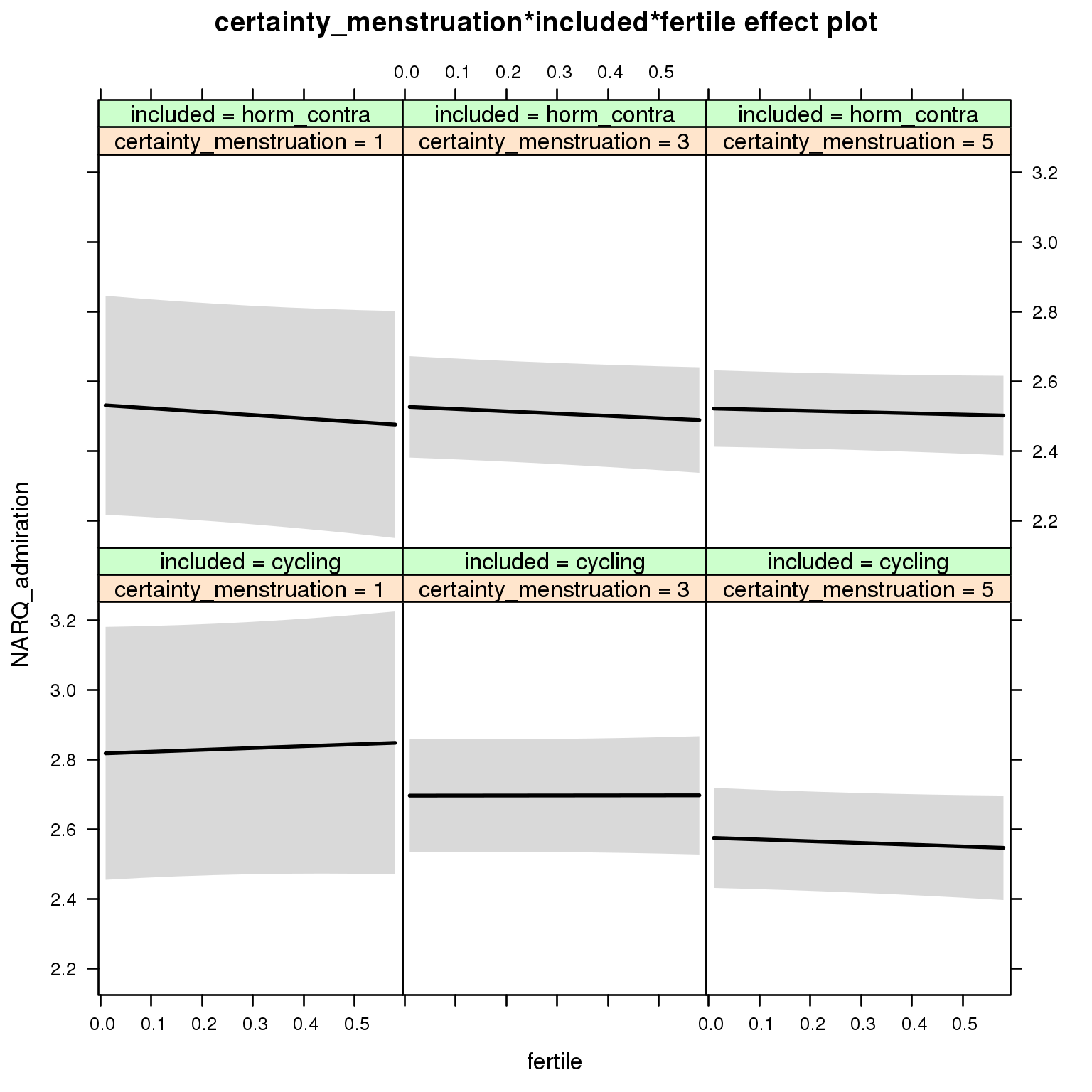
Linear mixed model fit by REML ['lmerMod']
Formula: NARQ_admiration ~ menstruation + fertile_mean + (1 | person) +
certainty_menstruation + included + fertile + menstruation:included +
certainty_menstruation:included + certainty_menstruation:fertile +
included:fertile + certainty_menstruation:included:fertile
Data: diary
REML criterion at convergence: 63034
Scaled residuals:
Min 1Q Median 3Q Max
-5.227 -0.515 -0.073 0.531 5.957
Random effects:
Groups Name Variance Std.Dev.
person (Intercept) 1.140 1.068
Residual 0.535 0.732
Number of obs: 26682, groups: person, 1054
Fixed effects:
Estimate Std. Error t value
(Intercept) 2.8601 0.2491 11.48
menstruationpre -0.0489 0.0224 -2.18
menstruationyes -0.1005 0.0212 -4.75
fertile_mean 0.2496 0.3837 0.65
certainty_menstruation -0.0604 0.0568 -1.06
includedhorm_contra -0.3636 0.3166 -1.15
fertile 0.0785 0.1780 0.44
menstruationpre:includedhorm_contra 0.0400 0.0288 1.39
menstruationyes:includedhorm_contra 0.0836 0.0277 3.02
certainty_menstruation:includedhorm_contra 0.0579 0.0739 0.78
certainty_menstruation:fertile -0.0257 0.0417 -0.62
includedhorm_contra:fertile -0.1906 0.2314 -0.82
certainty_menstruation:includedhorm_contra:fertile 0.0410 0.0535 0.77
M_m8: Moderation by cycle regularity
model %>%
test_moderator("cycle_regularity", diary)refitting model(s) with ML (instead of REML)
| Df | AIC | BIC | logLik | deviance | Chisq | Chi Df | Pr(>Chisq) | |
|---|---|---|---|---|---|---|---|---|
| with_main | 15 | 63000 | 63123 | -31485 | 62970 | NA | NA | NA |
| with_mod | 19 | 63007 | 63162 | -31484 | 62969 | 1.448 | 4 | 0.8359 |
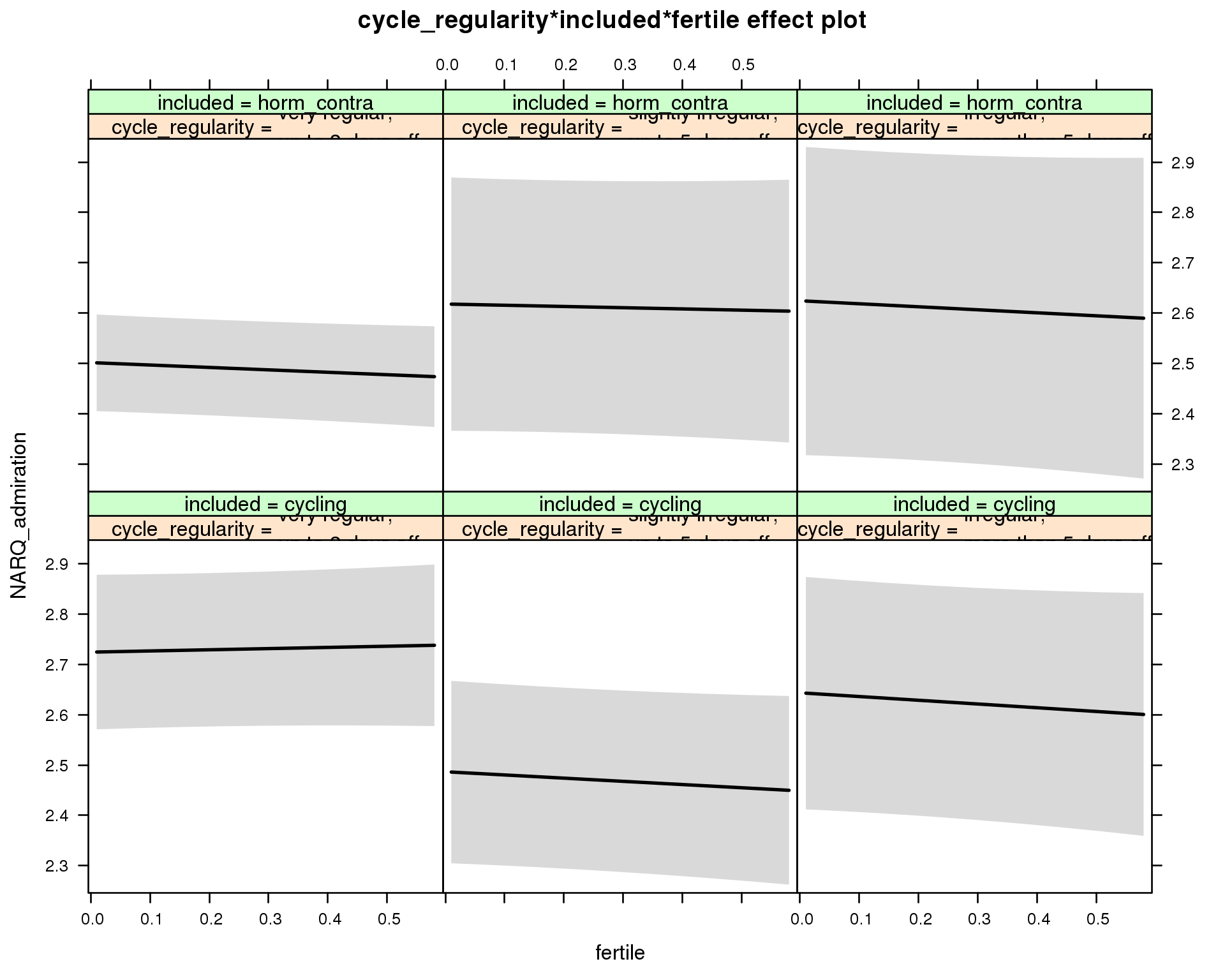
Linear mixed model fit by REML ['lmerMod']
Formula: NARQ_admiration ~ menstruation + fertile_mean + (1 | person) +
cycle_regularity + included + fertile + menstruation:included +
cycle_regularity:included + cycle_regularity:fertile + included:fertile +
cycle_regularity:included:fertile
Data: diary
REML criterion at convergence: 63031
Scaled residuals:
Min 1Q Median 3Q Max
-5.218 -0.516 -0.073 0.531 5.955
Random effects:
Groups Name Variance Std.Dev.
person (Intercept) 1.137 1.066
Residual 0.535 0.732
Number of obs: 26682, groups: person, 1054
Fixed effects:
Estimate Std. Error t value
(Intercept) 2.6899 0.1010 26.62
menstruationpre -0.0476 0.0224 -2.12
menstruationyes -0.0992 0.0211 -4.69
fertile_mean 0.3472 0.3850 0.90
cycle_regularityslightly irregular,\nup to 5 days off -0.2378 0.1214 -1.96
cycle_regularityirregular,\nmore than 5 days off -0.0808 0.1414 -0.57
includedhorm_contra -0.2442 0.0934 -2.61
fertile 0.0234 0.0626 0.37
menstruationpre:includedhorm_contra 0.0387 0.0288 1.35
menstruationyes:includedhorm_contra 0.0821 0.0277 2.96
cycle_regularityslightly irregular,\nup to 5 days off:includedhorm_contra 0.3542 0.1838 1.93
cycle_regularityirregular,\nmore than 5 days off:includedhorm_contra 0.2038 0.2165 0.94
cycle_regularityslightly irregular,\nup to 5 days off:fertile -0.0870 0.0864 -1.01
cycle_regularityirregular,\nmore than 5 days off:fertile -0.0977 0.1063 -0.92
includedhorm_contra:fertile -0.0716 0.0734 -0.98
cycle_regularityslightly irregular,\nup to 5 days off:includedhorm_contra:fertile 0.1109 0.1282 0.86
cycle_regularityirregular,\nmore than 5 days off:includedhorm_contra:fertile 0.0860 0.1585 0.54
M_m9: Moderation by cohabitation status
model %>%
test_moderator("cohabitation", diary)refitting model(s) with ML (instead of REML)
| Df | AIC | BIC | logLik | deviance | Chisq | Chi Df | Pr(>Chisq) | |
|---|---|---|---|---|---|---|---|---|
| with_main | 15 | 63004 | 63127 | -31487 | 62974 | NA | NA | NA |
| with_mod | 19 | 62987 | 63143 | -31475 | 62949 | 24.67 | 4 | 0.00005864 |
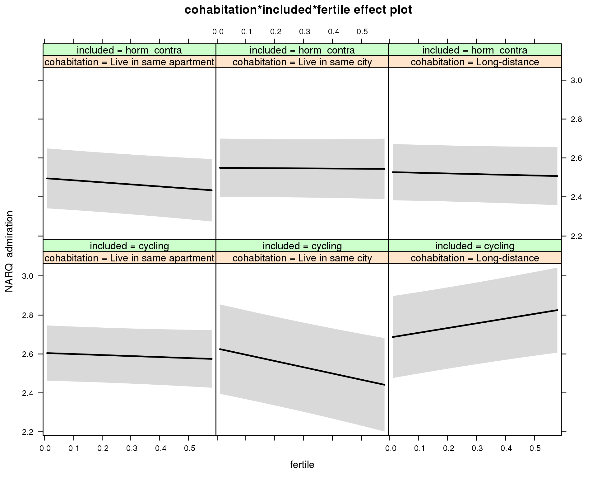
Linear mixed model fit by REML ['lmerMod']
Formula: NARQ_admiration ~ menstruation + fertile_mean + (1 | person) +
cohabitation + included + fertile + menstruation:included +
cohabitation:included + cohabitation:fertile + included:fertile + cohabitation:included:fertile
Data: diary
REML criterion at convergence: 63015
Scaled residuals:
Min 1Q Median 3Q Max
-5.231 -0.517 -0.073 0.530 5.962
Random effects:
Groups Name Variance Std.Dev.
person (Intercept) 1.142 1.069
Residual 0.535 0.731
Number of obs: 26682, groups: person, 1054
Fixed effects:
Estimate Std. Error t value
(Intercept) 2.5894 0.0981 26.38
menstruationpre -0.0492 0.0224 -2.20
menstruationyes -0.1017 0.0211 -4.82
fertile_mean 0.2418 0.3842 0.63
cohabitationLive in same city 0.0230 0.1376 0.17
cohabitationLong-distance 0.0795 0.1294 0.61
includedhorm_contra -0.1303 0.1074 -1.21
fertile -0.0523 0.0565 -0.93
menstruationpre:includedhorm_contra 0.0404 0.0287 1.41
menstruationyes:includedhorm_contra 0.0845 0.0277 3.05
cohabitationLive in same city:includedhorm_contra 0.0301 0.1760 0.17
cohabitationLong-distance:includedhorm_contra -0.0483 0.1683 -0.29
cohabitationLive in same city:fertile -0.2686 0.1034 -2.60
cohabitationLong-distance:fertile 0.2944 0.0931 3.16
includedhorm_contra:fertile -0.0544 0.0826 -0.66
cohabitationLive in same city:includedhorm_contra:fertile 0.3657 0.1292 2.83
cohabitationLong-distance:includedhorm_contra:fertile -0.2228 0.1198 -1.86
M_m10: Moderation by relationship status
model %>%
test_moderator("relationship_status_clean", diary)refitting model(s) with ML (instead of REML)
| Df | AIC | BIC | logLik | deviance | Chisq | Chi Df | Pr(>Chisq) | |
|---|---|---|---|---|---|---|---|---|
| with_main | 15 | 63005 | 63128 | -31487 | 62975 | NA | NA | NA |
| with_mod | 19 | 63009 | 63165 | -31486 | 62971 | 3.405 | 4 | 0.4924 |
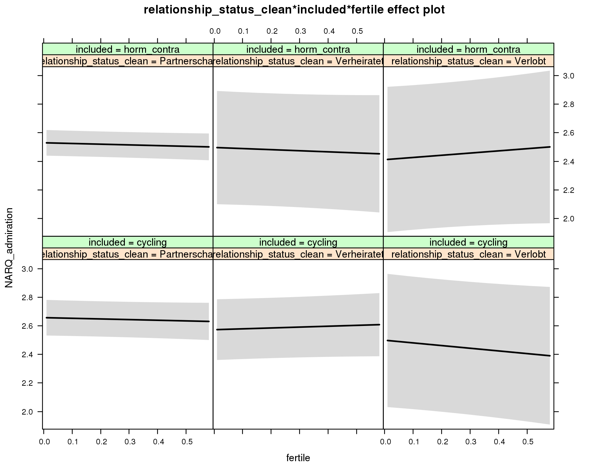
Linear mixed model fit by REML ['lmerMod']
Formula: NARQ_admiration ~ menstruation + fertile_mean + (1 | person) +
relationship_status_clean + included + fertile + menstruation:included +
relationship_status_clean:included + relationship_status_clean:fertile +
included:fertile + relationship_status_clean:included:fertile
Data: diary
REML criterion at convergence: 63028
Scaled residuals:
Min 1Q Median 3Q Max
-5.228 -0.516 -0.072 0.531 5.955
Random effects:
Groups Name Variance Std.Dev.
person (Intercept) 1.143 1.069
Residual 0.535 0.732
Number of obs: 26682, groups: person, 1054
Fixed effects:
Estimate Std. Error t value
(Intercept) 2.63992 0.09189 28.73
menstruationpre -0.04862 0.02240 -2.17
menstruationyes -0.09978 0.02112 -4.72
fertile_mean 0.24831 0.38407 0.65
relationship_status_cleanVerheiratet -0.08440 0.12565 -0.67
relationship_status_cleanVerlobt -0.15799 0.24620 -0.64
includedhorm_contra -0.14886 0.07937 -1.88
fertile -0.04552 0.05177 -0.88
menstruationpre:includedhorm_contra 0.03969 0.02875 1.38
menstruationyes:includedhorm_contra 0.08290 0.02769 2.99
relationship_status_cleanVerheiratet:includedhorm_contra 0.05150 0.24254 0.21
relationship_status_cleanVerlobt:includedhorm_contra 0.03986 0.36068 0.11
relationship_status_cleanVerheiratet:fertile 0.10640 0.09115 1.17
relationship_status_cleanVerlobt:fertile -0.14170 0.17099 -0.83
includedhorm_contra:fertile -0.00396 0.06317 -0.06
relationship_status_cleanVerheiratet:includedhorm_contra:fertile -0.13315 0.17165 -0.78
relationship_status_cleanVerlobt:includedhorm_contra:fertile 0.34489 0.26542 1.30
Narcisstic rivalry
model_summaries$NARQ_rivalryModel summary
Model summary
model %>%
print_summary()Linear mixed model fit by REML
t-tests use Satterthwaite approximations to degrees of freedom ['lmerMod']
Formula: NARQ_rivalry ~ included * (menstruation + fertile) + fertile_mean + (1 | person)
Data: diary
REML criterion at convergence: 41866
Scaled residuals:
Min 1Q Median 3Q Max
-4.965 -0.328 -0.090 -0.011 9.684
Random effects:
Groups Name Variance Std.Dev.
person (Intercept) 0.240 0.490
Residual 0.249 0.499
Number of obs: 26681, groups: person, 1054
Fixed effects:
Estimate Std. Error df t value Pr(>|t|)
(Intercept) 1.293491 0.041281 1299.000000 31.33 <2e-16 ***
includedhorm_contra 0.038593 0.033891 1248.000000 1.14 0.26
menstruationpre -0.017936 0.015262 25894.000000 -1.18 0.24
menstruationyes 0.004104 0.014389 25989.000000 0.29 0.78
fertile -0.021982 0.030799 25888.000000 -0.71 0.48
fertile_mean 0.082770 0.188205 1408.000000 0.44 0.66
includedhorm_contra:menstruationpre 0.000364 0.019594 25890.000000 0.02 0.99
includedhorm_contra:menstruationyes -0.019740 0.018860 25970.000000 -1.05 0.30
includedhorm_contra:fertile -0.027179 0.039036 25995.000000 -0.70 0.49
---
Signif. codes: 0 '***' 0.001 '**' 0.01 '*' 0.05 '.' 0.1 ' ' 1
Correlation of Fixed Effects:
(Intr) incld_ mnstrtnp mnstrtny fertil frtl_m inclddhrm_cntr:mnstrtnp
inclddhrm_c -0.474
menstrutnpr -0.141 0.179
menstrutnys -0.138 0.173 0.398
fertile -0.136 0.223 0.467 0.385
fertile_men -0.772 -0.024 -0.008 -0.005 -0.059
inclddhrm_cntr:mnstrtnp 0.117 -0.225 -0.779 -0.310 -0.363 -0.003
inclddhrm_cntr:mnstrtny 0.111 -0.213 -0.303 -0.763 -0.293 -0.003 0.384
inclddhrm_cntr:f 0.136 -0.281 -0.368 -0.303 -0.787 0.010 0.467
inclddhrm_cntr:mnstrtny
inclddhrm_c
menstrutnpr
menstrutnys
fertile
fertile_men
inclddhrm_cntr:mnstrtnp
inclddhrm_cntr:mnstrtny
inclddhrm_cntr:f 0.382
Effect size standardised by residual variance (\(\frac{b}{ SD_{residual} }\)): -0.04 [-0.16;0.08].
Marginal effect plots
model %>%
plot_all_effects()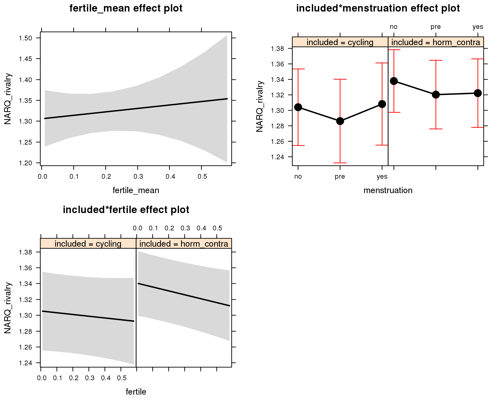
Outcome distribution
model %>%
plot_outcome(diary) + xlab(outcome_label)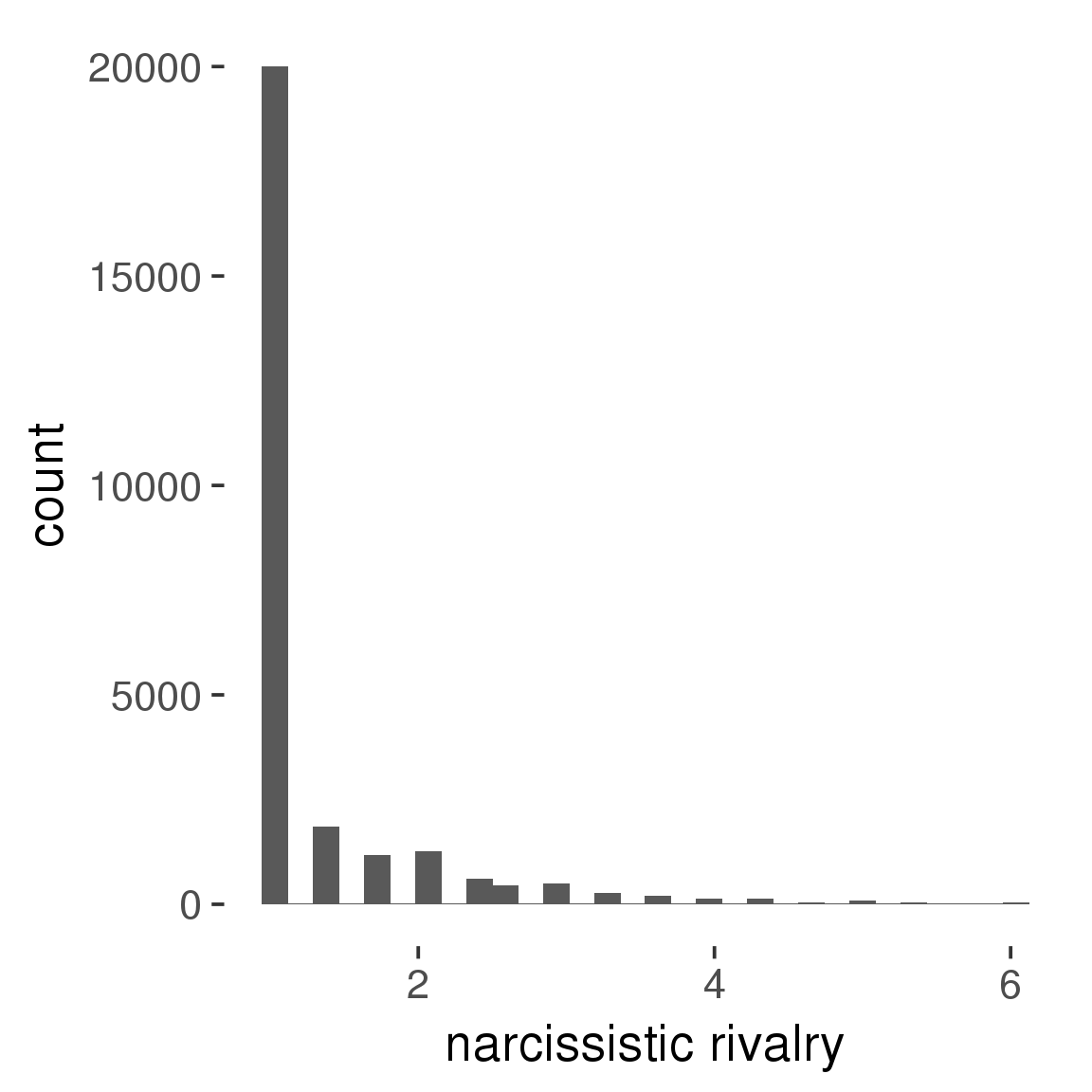
Diagnostics
model %>%
print_diagnostics()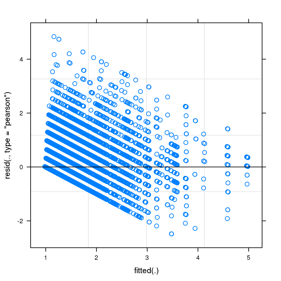
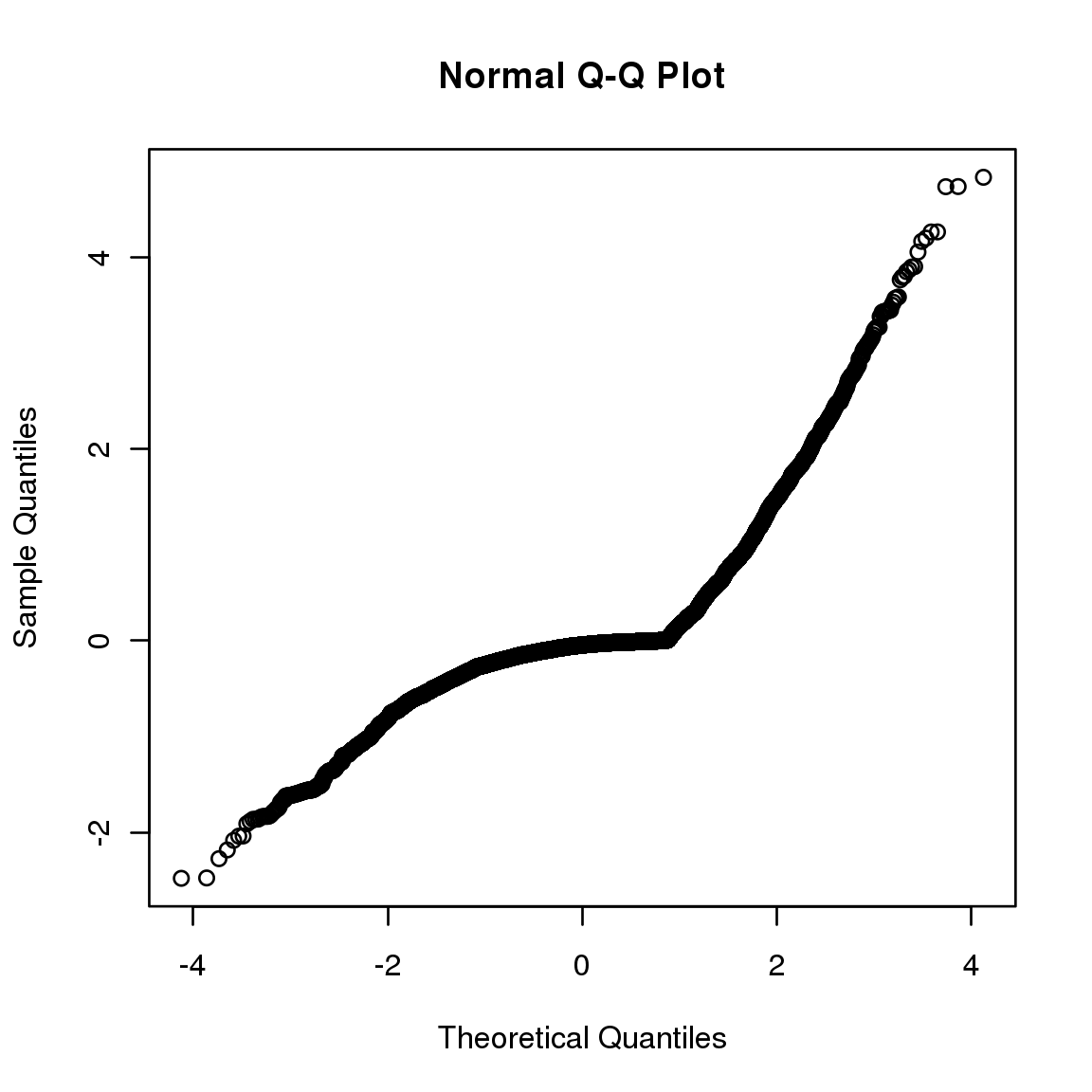

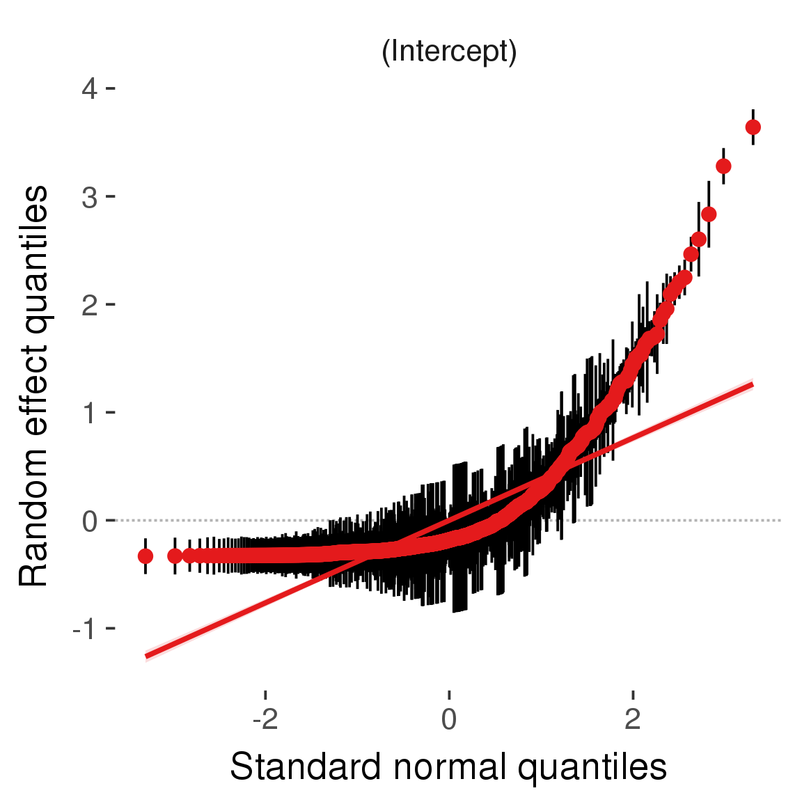
Curves
Here, we continuously plot the outcome over the course of the cycle. Because cycle lengths vary, we subset the data to cycles in a certain range. If the red curve traces the pink curve, our predictor accurately maps the relationship between fertile window probability and the outcome.
Cycle lengths from 21 to 36
Backward-counted
model %>%
plot_curve(diary %>% filter(minimum_cycle_length_diary <= 36, minimum_cycle_length_diary > 20) %>% mutate(fertile=prc_stirn_b))outcome = names(model@frame)[1]
outcome_label = recode(str_replace_all(str_replace_all(str_replace_all(outcome, "_", " "), " pair", "-pair"), " 1", ""),
"desirability 1" = "self-perceived desirability",
"NARQ admiration" = "narcissistic admiration",
"NARQ rivalry" = "narcissistic rivalry",
"extra-pair" = "extra-pair desire & behaviour",
"had sexual intercourse" = "sexual intercourse")
library(ggplot2)
# form a subset and run the model without the hormonal contraception and the fertility predictors
tmp = diary %>%
filter(!is.na(fertile), !is.na(included),
RCD > -1 * minimum_cycle_length_diary, RCD > -40)
new_form = update.formula(formula(model), new = . ~ . - fertile * included)
tmp$residuals = residuals(update(model, new_form, data = tmp , na.action = na.exclude))
tmp = tmp %>%
filter(!is.na(RCD), !is.na(residuals))
rcd_min = min(tmp$RCD)
tmp$real = FALSE
tmp_before = tmp
tmp_before$RCD = tmp_before$RCD + min(tmp$RCD) - 1
tmp_after = tmp
tmp_after$RCD = tmp_after$RCD - min(tmp$RCD) + 1
tmp$real = TRUE
tmp = bind_rows(tmp_before %>% filter(RCD > rcd_min - 11), tmp, tmp_after %>% filter(RCD < 11))GAM smooth on residuals
Here, we partialled out menstruation and individual random effects, then superimposed estimated probability of being in the fertile window scaled to the range of the estimated means. To address the periodicity of the cycle, we prepended and appended ten days of the timeseries to the end and the beginning of the timeseries. We then estimated the GAM and cut off the appended subsets before plotting.
tryCatch({
trend_plot = ggplot(tmp,aes(x = RCD, y = residuals, colour = included)) +
stat_smooth(geom = 'smooth',size = 0.8, fill = "#9ECAE1", method = 'gam', formula = y ~ s(x))
}, error = function(e){cat_message(e, "danger")})
tryCatch({
trend_data = ggplot_build(trend_plot)$data[[1]]
}, error = function(e){cat_message(e, "danger")})
trend_data$RCD = round(trend_data$x)
trend_data = left_join(trend_data, tmp %>% select(real, RCD,fertile) %>% unique(), by = "RCD")
trend_data %>%
filter(real == TRUE) %>%
mutate(superimposed = ( ( (fertile - 0.01)/0.58) * (max(y)-min(y) ) ) + min(y) ) ->
trend_data
ggplot(trend_data) +
geom_ribbon(aes(x = x, ymin = ymin, ymax = ymax, fill = factor(group)), alpha = 0.2) +
geom_line(aes(x = x, y = y, colour = factor(group)), size = 0.8, stat = "identity") +
scale_x_continuous(caption_x) +
geom_line(aes(x = x, y = superimposed), color = "#a83fbf", size = 1, linetype = 'dashed') +
annotate("text",x = mean(trend_data$x), y = max(trend_data$superimposed,na.rm=T) + 0.1, label = 'superimposed fertility peak', color = "#a83fbf") +
scale_y_continuous(outcome_label) +
ggtitle("GAM smooth, residuals") +
scale_color_manual("Contraception status",values = c("2"="black","1"= "red"), labels = c("2"="hormonally\ncontracepting","1"="cycling"), guide = F) +
scale_fill_manual("Contraception status",values = c("2"="black","1"= "red"), labels = c("2"="hormonally\ncontracepting","1"="cycling"), guide = F)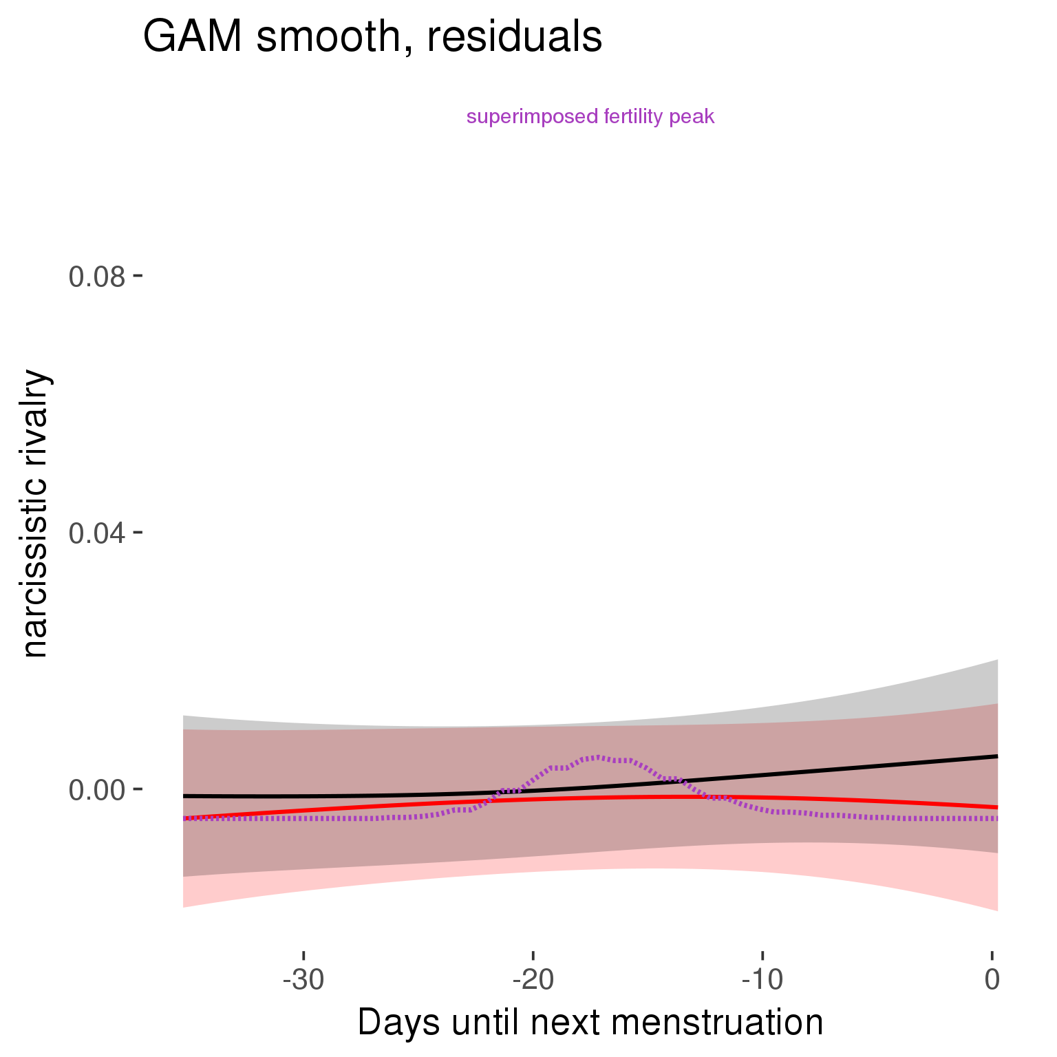
GAM smooth on raw data
As before, but without partialling anything out.
tryCatch({
trend_plot = ggplot(tmp,aes_string(x = "RCD", y = outcome, colour = "included")) +
stat_smooth(geom = 'smooth',size = 0.8, fill = "#9ECAE1", method = 'gam', formula = y ~ s(x))
}, error = function(e){cat_message(e, "danger")})
tryCatch({
trend_data = ggplot_build(trend_plot)$data[[1]]
}, error = function(e){cat_message(e, "danger")})
trend_data$RCD = round(trend_data$x)
trend_data = left_join(trend_data, tmp %>% select(real, RCD,fertile) %>% unique(), by = "RCD")
trend_data %>%
filter(real == TRUE) %>%
mutate(superimposed = ( ( (fertile - 0.01)/0.58) * (max(y)-min(y) ) ) + min(y) ) ->
trend_data
plot1b = ggplot(trend_data) +
geom_ribbon(aes(x = x, ymin = ymin, ymax = ymax, fill = factor(group)), alpha = 0.2) +
geom_line(aes(x = x, y = y, colour = factor(group)), size = 0.8, stat = "identity") +
scale_x_continuous(caption_x) +
geom_line(aes(x = x, y = superimposed), color = "#a83fbf", size = 1, linetype = 'dashed') +
annotate("text",x = mean(trend_data$x), y = max(trend_data$superimposed,na.rm=T) + 0.1, label = 'superimposed fertility peak', color = "#a83fbf") +
scale_y_continuous(outcome_label) +
ggtitle("GAM smooth, raw data") +
scale_color_manual("Contraception status",values = c("2"="black","1"= "red"), labels = c("2"="hormonally\ncontracepting","1"="cycling"), guide = F) +
scale_fill_manual("Contraception status",values = c("2"="black","1"= "red"), labels = c("2"="hormonally\ncontracepting","1"="cycling"), guide = F)
suppressWarnings(print(plot1b))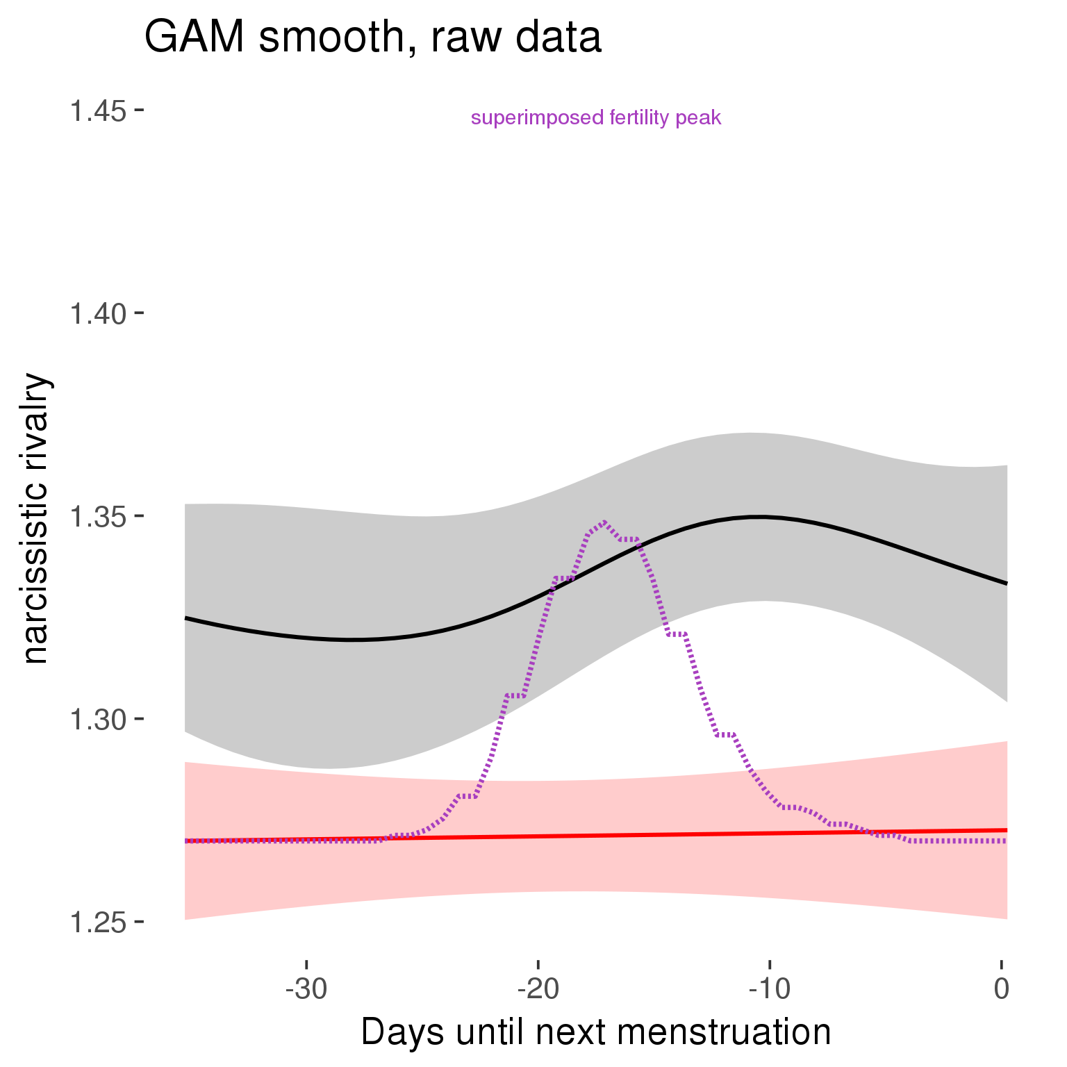
Means and standard errors over raw data
Nothing partialled out, just straight means with bootstrapped confidence intervals.
tryCatch({
trend_plot = ggplot(tmp,aes_string(x = "RCD", y = outcome, colour = "included")) +
geom_pointrange(size = 0.8, stat = 'summary', fun.data = "mean_cl_boot")
}, error = function(e){cat_message(e, "danger")})
tryCatch({
trend_data = ggplot_build(trend_plot)$data[[1]]
}, error = function(e){cat_message(e, "danger")})
trend_data$RCD = round(trend_data$x)
trend_data = left_join(trend_data, tmp %>% select(real, RCD,fertile) %>% unique(), by = "RCD")
trend_data %>%
filter(real == TRUE) %>%
mutate(superimposed = ( ( (fertile - 0.01)/0.58) * (max(y)-min(y) ) ) + min(y) ) ->
trend_data
plot3 = ggplot(trend_data) +
geom_pointrange(aes(x = x, y = y, ymin = ymin,ymax = ymax, colour = factor(group)), size = 0.8, stat = "identity", alpha = 0.6, position = position_dodge(width = .5)) +
scale_x_continuous("Days until next menstruation") +
geom_line(aes(x= x, y = superimposed), color = "#a83fbf", size = 1, linetype = 'dashed') +
annotate("text",x = mean(trend_data$x), y = max(trend_data$superimposed,na.rm=T) + 0.1, label = 'superimposed fertility peak', color = "#a83fbf") +
scale_y_continuous(outcome_label) +
ggtitle("Means with standard errors, raw data") +
scale_color_manual("Contraception status",values = c("2"="black","1"= "red"), labels = c("2"="hormonally\ncontracepting","1"="cycling"), guide = F) +
scale_fill_manual("Contraception status",values = c("2"="black","1"= "red"), labels = c("2"="hormonally\ncontracepting","1"="cycling"), guide = F)
suppressWarnings(print(plot3))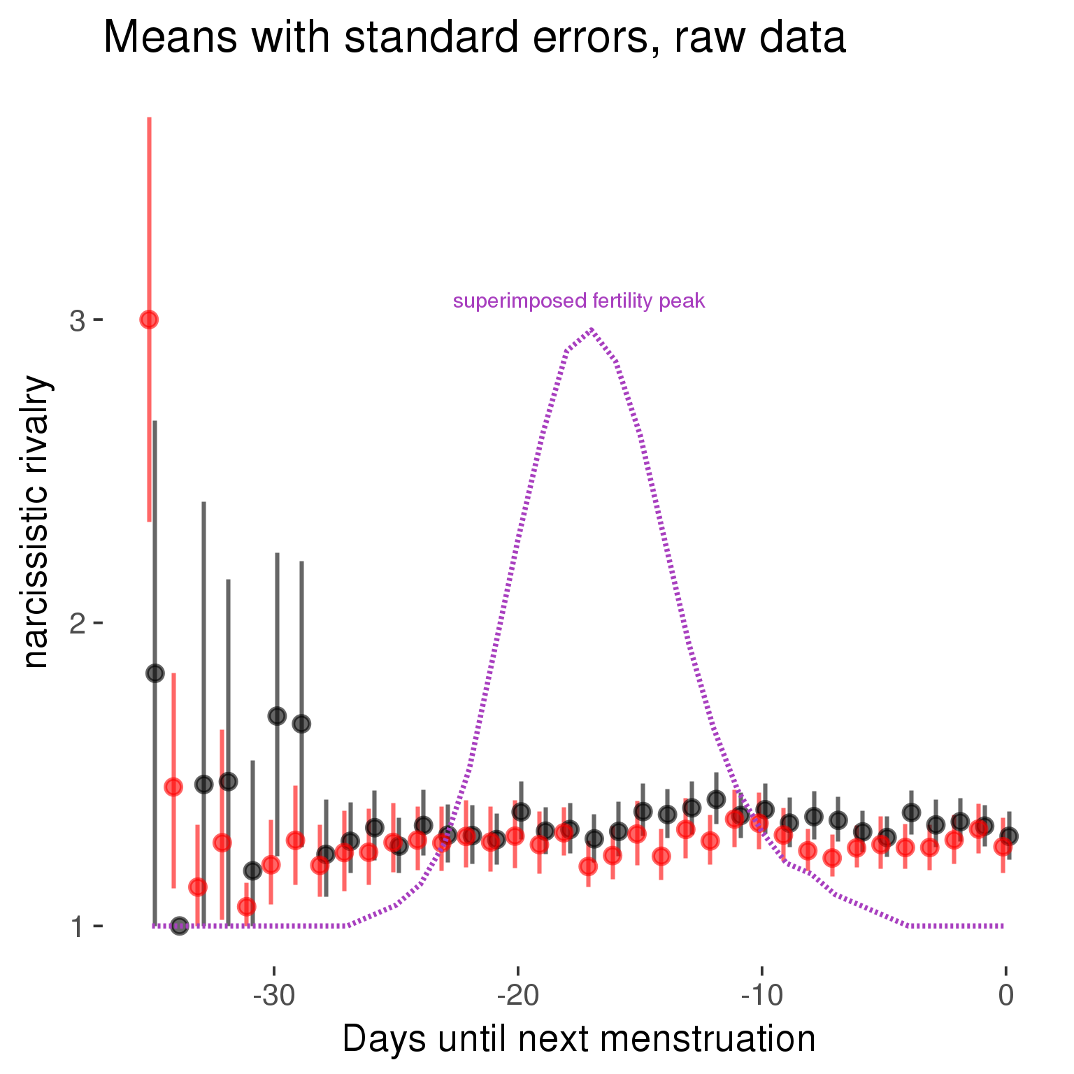
Forward-counted
model %>%
plot_curve(diary %>% filter(minimum_cycle_length_diary <= 36, minimum_cycle_length_diary > 20) %>% mutate(RCD = FCD, fertile = prc_stirn_b_forward_counted), caption_x = "Days since last menstruation")outcome = names(model@frame)[1]
outcome_label = recode(str_replace_all(str_replace_all(str_replace_all(outcome, "_", " "), " pair", "-pair"), " 1", ""),
"desirability 1" = "self-perceived desirability",
"NARQ admiration" = "narcissistic admiration",
"NARQ rivalry" = "narcissistic rivalry",
"extra-pair" = "extra-pair desire & behaviour",
"had sexual intercourse" = "sexual intercourse")
library(ggplot2)
# form a subset and run the model without the hormonal contraception and the fertility predictors
tmp = diary %>%
filter(!is.na(fertile), !is.na(included),
RCD > -1 * minimum_cycle_length_diary, RCD > -40)
new_form = update.formula(formula(model), new = . ~ . - fertile * included)
tmp$residuals = residuals(update(model, new_form, data = tmp , na.action = na.exclude))
tmp = tmp %>%
filter(!is.na(RCD), !is.na(residuals))
rcd_min = min(tmp$RCD)
tmp$real = FALSE
tmp_before = tmp
tmp_before$RCD = tmp_before$RCD + min(tmp$RCD) - 1
tmp_after = tmp
tmp_after$RCD = tmp_after$RCD - min(tmp$RCD) + 1
tmp$real = TRUE
tmp = bind_rows(tmp_before %>% filter(RCD > rcd_min - 11), tmp, tmp_after %>% filter(RCD < 11))GAM smooth on residuals
Here, we partialled out menstruation and individual random effects, then superimposed estimated probability of being in the fertile window scaled to the range of the estimated means. To address the periodicity of the cycle, we prepended and appended ten days of the timeseries to the end and the beginning of the timeseries. We then estimated the GAM and cut off the appended subsets before plotting.
tryCatch({
trend_plot = ggplot(tmp,aes(x = RCD, y = residuals, colour = included)) +
stat_smooth(geom = 'smooth',size = 0.8, fill = "#9ECAE1", method = 'gam', formula = y ~ s(x))
}, error = function(e){cat_message(e, "danger")})
tryCatch({
trend_data = ggplot_build(trend_plot)$data[[1]]
}, error = function(e){cat_message(e, "danger")})
trend_data$RCD = round(trend_data$x)
trend_data = left_join(trend_data, tmp %>% select(real, RCD,fertile) %>% unique(), by = "RCD")
trend_data %>%
filter(real == TRUE) %>%
mutate(superimposed = ( ( (fertile - 0.01)/0.58) * (max(y)-min(y) ) ) + min(y) ) ->
trend_data
ggplot(trend_data) +
geom_ribbon(aes(x = x, ymin = ymin, ymax = ymax, fill = factor(group)), alpha = 0.2) +
geom_line(aes(x = x, y = y, colour = factor(group)), size = 0.8, stat = "identity") +
scale_x_continuous(caption_x) +
geom_line(aes(x = x, y = superimposed), color = "#a83fbf", size = 1, linetype = 'dashed') +
annotate("text",x = mean(trend_data$x), y = max(trend_data$superimposed,na.rm=T) + 0.1, label = 'superimposed fertility peak', color = "#a83fbf") +
scale_y_continuous(outcome_label) +
ggtitle("GAM smooth, residuals") +
scale_color_manual("Contraception status",values = c("2"="black","1"= "red"), labels = c("2"="hormonally\ncontracepting","1"="cycling"), guide = F) +
scale_fill_manual("Contraception status",values = c("2"="black","1"= "red"), labels = c("2"="hormonally\ncontracepting","1"="cycling"), guide = F)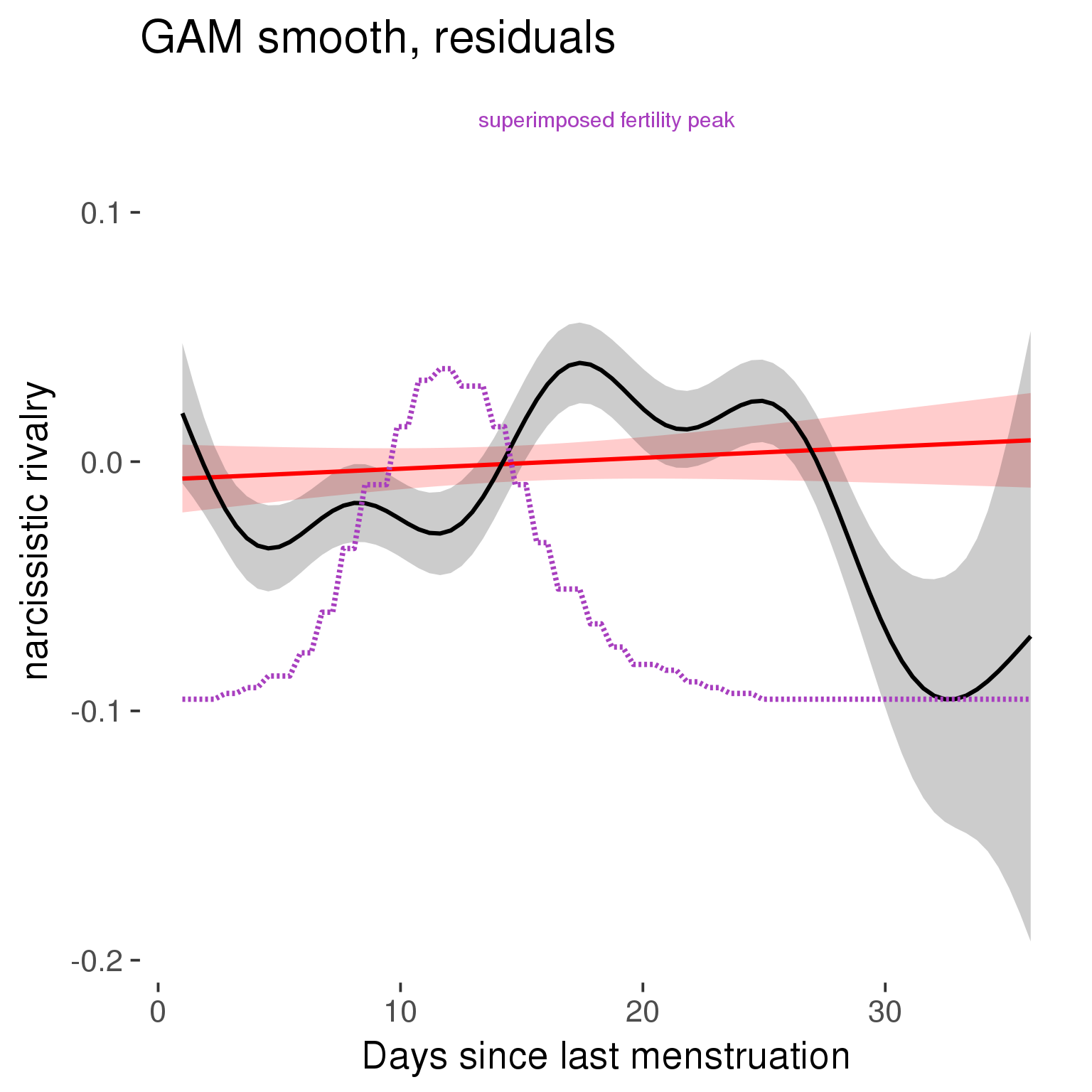
GAM smooth on raw data
As before, but without partialling anything out.
tryCatch({
trend_plot = ggplot(tmp,aes_string(x = "RCD", y = outcome, colour = "included")) +
stat_smooth(geom = 'smooth',size = 0.8, fill = "#9ECAE1", method = 'gam', formula = y ~ s(x))
}, error = function(e){cat_message(e, "danger")})
tryCatch({
trend_data = ggplot_build(trend_plot)$data[[1]]
}, error = function(e){cat_message(e, "danger")})
trend_data$RCD = round(trend_data$x)
trend_data = left_join(trend_data, tmp %>% select(real, RCD,fertile) %>% unique(), by = "RCD")
trend_data %>%
filter(real == TRUE) %>%
mutate(superimposed = ( ( (fertile - 0.01)/0.58) * (max(y)-min(y) ) ) + min(y) ) ->
trend_data
plot1b = ggplot(trend_data) +
geom_ribbon(aes(x = x, ymin = ymin, ymax = ymax, fill = factor(group)), alpha = 0.2) +
geom_line(aes(x = x, y = y, colour = factor(group)), size = 0.8, stat = "identity") +
scale_x_continuous(caption_x) +
geom_line(aes(x = x, y = superimposed), color = "#a83fbf", size = 1, linetype = 'dashed') +
annotate("text",x = mean(trend_data$x), y = max(trend_data$superimposed,na.rm=T) + 0.1, label = 'superimposed fertility peak', color = "#a83fbf") +
scale_y_continuous(outcome_label) +
ggtitle("GAM smooth, raw data") +
scale_color_manual("Contraception status",values = c("2"="black","1"= "red"), labels = c("2"="hormonally\ncontracepting","1"="cycling"), guide = F) +
scale_fill_manual("Contraception status",values = c("2"="black","1"= "red"), labels = c("2"="hormonally\ncontracepting","1"="cycling"), guide = F)
suppressWarnings(print(plot1b))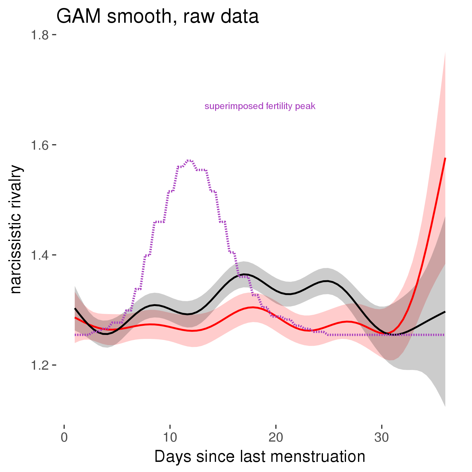
Means and standard errors over raw data
Nothing partialled out, just straight means with bootstrapped confidence intervals.
tryCatch({
trend_plot = ggplot(tmp,aes_string(x = "RCD", y = outcome, colour = "included")) +
geom_pointrange(size = 0.8, stat = 'summary', fun.data = "mean_cl_boot")
}, error = function(e){cat_message(e, "danger")})
tryCatch({
trend_data = ggplot_build(trend_plot)$data[[1]]
}, error = function(e){cat_message(e, "danger")})
trend_data$RCD = round(trend_data$x)
trend_data = left_join(trend_data, tmp %>% select(real, RCD,fertile) %>% unique(), by = "RCD")
trend_data %>%
filter(real == TRUE) %>%
mutate(superimposed = ( ( (fertile - 0.01)/0.58) * (max(y)-min(y) ) ) + min(y) ) ->
trend_data
plot3 = ggplot(trend_data) +
geom_pointrange(aes(x = x, y = y, ymin = ymin,ymax = ymax, colour = factor(group)), size = 0.8, stat = "identity", alpha = 0.6, position = position_dodge(width = .5)) +
scale_x_continuous("Days until next menstruation") +
geom_line(aes(x= x, y = superimposed), color = "#a83fbf", size = 1, linetype = 'dashed') +
annotate("text",x = mean(trend_data$x), y = max(trend_data$superimposed,na.rm=T) + 0.1, label = 'superimposed fertility peak', color = "#a83fbf") +
scale_y_continuous(outcome_label) +
ggtitle("Means with standard errors, raw data") +
scale_color_manual("Contraception status",values = c("2"="black","1"= "red"), labels = c("2"="hormonally\ncontracepting","1"="cycling"), guide = F) +
scale_fill_manual("Contraception status",values = c("2"="black","1"= "red"), labels = c("2"="hormonally\ncontracepting","1"="cycling"), guide = F)
suppressWarnings(print(plot3))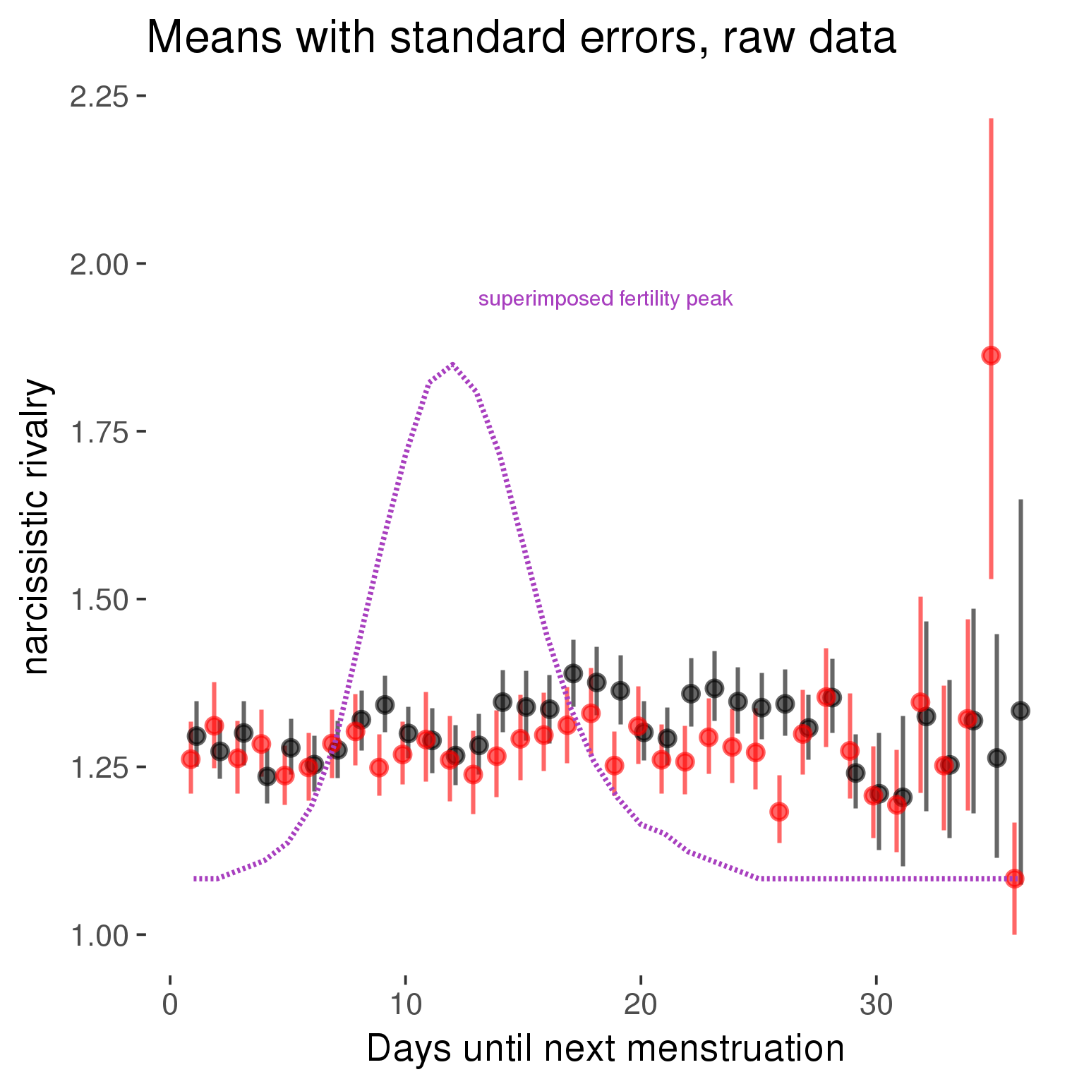
Cycle lengths from 27 to 30
Backward-counted
model %>%
plot_curve(diary %>% filter(minimum_cycle_length_diary <= 30, minimum_cycle_length_diary >= 27) %>% mutate(fertile=prc_stirn_b))outcome = names(model@frame)[1]
outcome_label = recode(str_replace_all(str_replace_all(str_replace_all(outcome, "_", " "), " pair", "-pair"), " 1", ""),
"desirability 1" = "self-perceived desirability",
"NARQ admiration" = "narcissistic admiration",
"NARQ rivalry" = "narcissistic rivalry",
"extra-pair" = "extra-pair desire & behaviour",
"had sexual intercourse" = "sexual intercourse")
library(ggplot2)
# form a subset and run the model without the hormonal contraception and the fertility predictors
tmp = diary %>%
filter(!is.na(fertile), !is.na(included),
RCD > -1 * minimum_cycle_length_diary, RCD > -40)
new_form = update.formula(formula(model), new = . ~ . - fertile * included)
tmp$residuals = residuals(update(model, new_form, data = tmp , na.action = na.exclude))
tmp = tmp %>%
filter(!is.na(RCD), !is.na(residuals))
rcd_min = min(tmp$RCD)
tmp$real = FALSE
tmp_before = tmp
tmp_before$RCD = tmp_before$RCD + min(tmp$RCD) - 1
tmp_after = tmp
tmp_after$RCD = tmp_after$RCD - min(tmp$RCD) + 1
tmp$real = TRUE
tmp = bind_rows(tmp_before %>% filter(RCD > rcd_min - 11), tmp, tmp_after %>% filter(RCD < 11))GAM smooth on residuals
Here, we partialled out menstruation and individual random effects, then superimposed estimated probability of being in the fertile window scaled to the range of the estimated means. To address the periodicity of the cycle, we prepended and appended ten days of the timeseries to the end and the beginning of the timeseries. We then estimated the GAM and cut off the appended subsets before plotting.
tryCatch({
trend_plot = ggplot(tmp,aes(x = RCD, y = residuals, colour = included)) +
stat_smooth(geom = 'smooth',size = 0.8, fill = "#9ECAE1", method = 'gam', formula = y ~ s(x))
}, error = function(e){cat_message(e, "danger")})
tryCatch({
trend_data = ggplot_build(trend_plot)$data[[1]]
}, error = function(e){cat_message(e, "danger")})
trend_data$RCD = round(trend_data$x)
trend_data = left_join(trend_data, tmp %>% select(real, RCD,fertile) %>% unique(), by = "RCD")
trend_data %>%
filter(real == TRUE) %>%
mutate(superimposed = ( ( (fertile - 0.01)/0.58) * (max(y)-min(y) ) ) + min(y) ) ->
trend_data
ggplot(trend_data) +
geom_ribbon(aes(x = x, ymin = ymin, ymax = ymax, fill = factor(group)), alpha = 0.2) +
geom_line(aes(x = x, y = y, colour = factor(group)), size = 0.8, stat = "identity") +
scale_x_continuous(caption_x) +
geom_line(aes(x = x, y = superimposed), color = "#a83fbf", size = 1, linetype = 'dashed') +
annotate("text",x = mean(trend_data$x), y = max(trend_data$superimposed,na.rm=T) + 0.1, label = 'superimposed fertility peak', color = "#a83fbf") +
scale_y_continuous(outcome_label) +
ggtitle("GAM smooth, residuals") +
scale_color_manual("Contraception status",values = c("2"="black","1"= "red"), labels = c("2"="hormonally\ncontracepting","1"="cycling"), guide = F) +
scale_fill_manual("Contraception status",values = c("2"="black","1"= "red"), labels = c("2"="hormonally\ncontracepting","1"="cycling"), guide = F)
GAM smooth on raw data
As before, but without partialling anything out.
tryCatch({
trend_plot = ggplot(tmp,aes_string(x = "RCD", y = outcome, colour = "included")) +
stat_smooth(geom = 'smooth',size = 0.8, fill = "#9ECAE1", method = 'gam', formula = y ~ s(x))
}, error = function(e){cat_message(e, "danger")})
tryCatch({
trend_data = ggplot_build(trend_plot)$data[[1]]
}, error = function(e){cat_message(e, "danger")})
trend_data$RCD = round(trend_data$x)
trend_data = left_join(trend_data, tmp %>% select(real, RCD,fertile) %>% unique(), by = "RCD")
trend_data %>%
filter(real == TRUE) %>%
mutate(superimposed = ( ( (fertile - 0.01)/0.58) * (max(y)-min(y) ) ) + min(y) ) ->
trend_data
plot1b = ggplot(trend_data) +
geom_ribbon(aes(x = x, ymin = ymin, ymax = ymax, fill = factor(group)), alpha = 0.2) +
geom_line(aes(x = x, y = y, colour = factor(group)), size = 0.8, stat = "identity") +
scale_x_continuous(caption_x) +
geom_line(aes(x = x, y = superimposed), color = "#a83fbf", size = 1, linetype = 'dashed') +
annotate("text",x = mean(trend_data$x), y = max(trend_data$superimposed,na.rm=T) + 0.1, label = 'superimposed fertility peak', color = "#a83fbf") +
scale_y_continuous(outcome_label) +
ggtitle("GAM smooth, raw data") +
scale_color_manual("Contraception status",values = c("2"="black","1"= "red"), labels = c("2"="hormonally\ncontracepting","1"="cycling"), guide = F) +
scale_fill_manual("Contraception status",values = c("2"="black","1"= "red"), labels = c("2"="hormonally\ncontracepting","1"="cycling"), guide = F)
suppressWarnings(print(plot1b))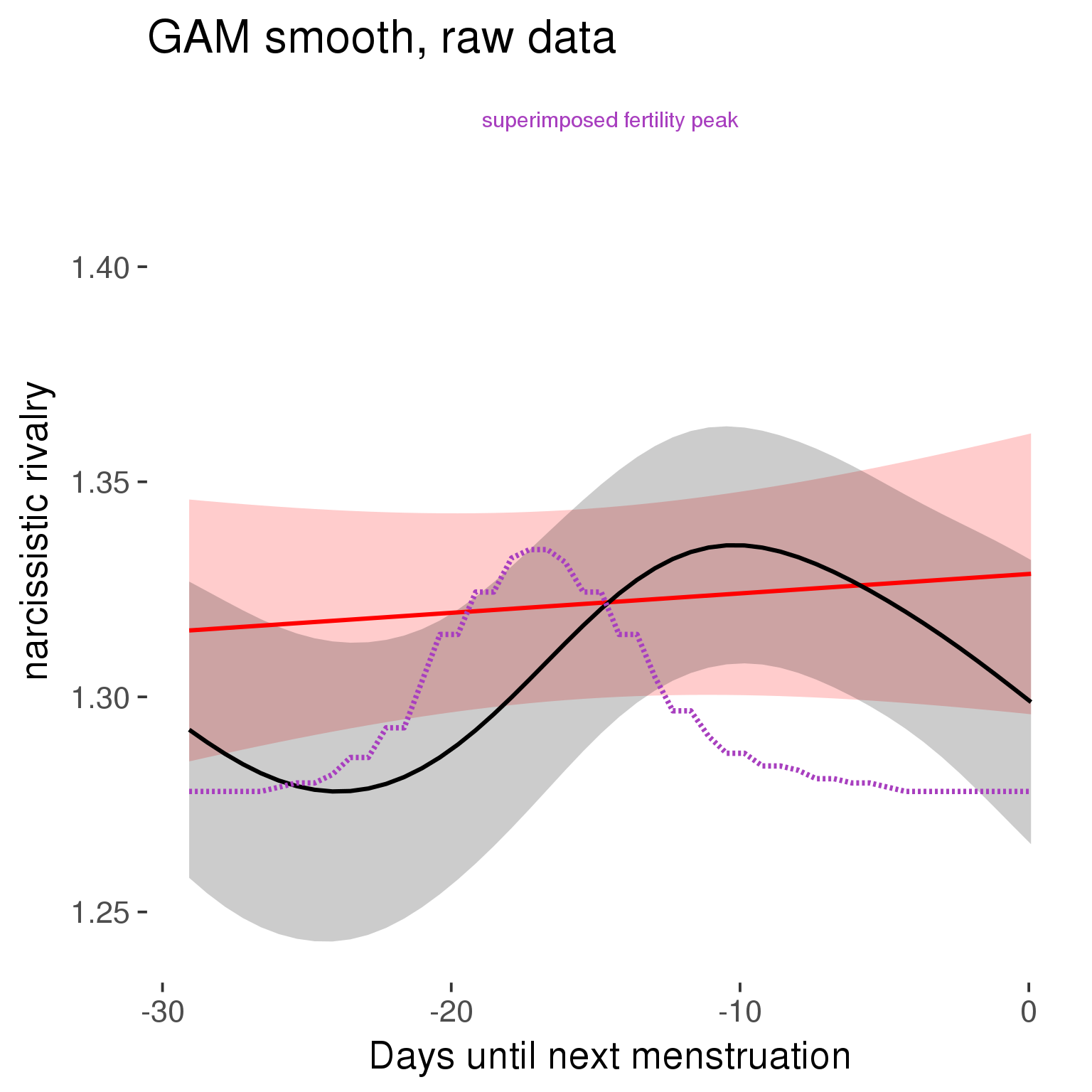
Means and standard errors over raw data
Nothing partialled out, just straight means with bootstrapped confidence intervals.
tryCatch({
trend_plot = ggplot(tmp,aes_string(x = "RCD", y = outcome, colour = "included")) +
geom_pointrange(size = 0.8, stat = 'summary', fun.data = "mean_cl_boot")
}, error = function(e){cat_message(e, "danger")})
tryCatch({
trend_data = ggplot_build(trend_plot)$data[[1]]
}, error = function(e){cat_message(e, "danger")})
trend_data$RCD = round(trend_data$x)
trend_data = left_join(trend_data, tmp %>% select(real, RCD,fertile) %>% unique(), by = "RCD")
trend_data %>%
filter(real == TRUE) %>%
mutate(superimposed = ( ( (fertile - 0.01)/0.58) * (max(y)-min(y) ) ) + min(y) ) ->
trend_data
plot3 = ggplot(trend_data) +
geom_pointrange(aes(x = x, y = y, ymin = ymin,ymax = ymax, colour = factor(group)), size = 0.8, stat = "identity", alpha = 0.6, position = position_dodge(width = .5)) +
scale_x_continuous("Days until next menstruation") +
geom_line(aes(x= x, y = superimposed), color = "#a83fbf", size = 1, linetype = 'dashed') +
annotate("text",x = mean(trend_data$x), y = max(trend_data$superimposed,na.rm=T) + 0.1, label = 'superimposed fertility peak', color = "#a83fbf") +
scale_y_continuous(outcome_label) +
ggtitle("Means with standard errors, raw data") +
scale_color_manual("Contraception status",values = c("2"="black","1"= "red"), labels = c("2"="hormonally\ncontracepting","1"="cycling"), guide = F) +
scale_fill_manual("Contraception status",values = c("2"="black","1"= "red"), labels = c("2"="hormonally\ncontracepting","1"="cycling"), guide = F)
suppressWarnings(print(plot3))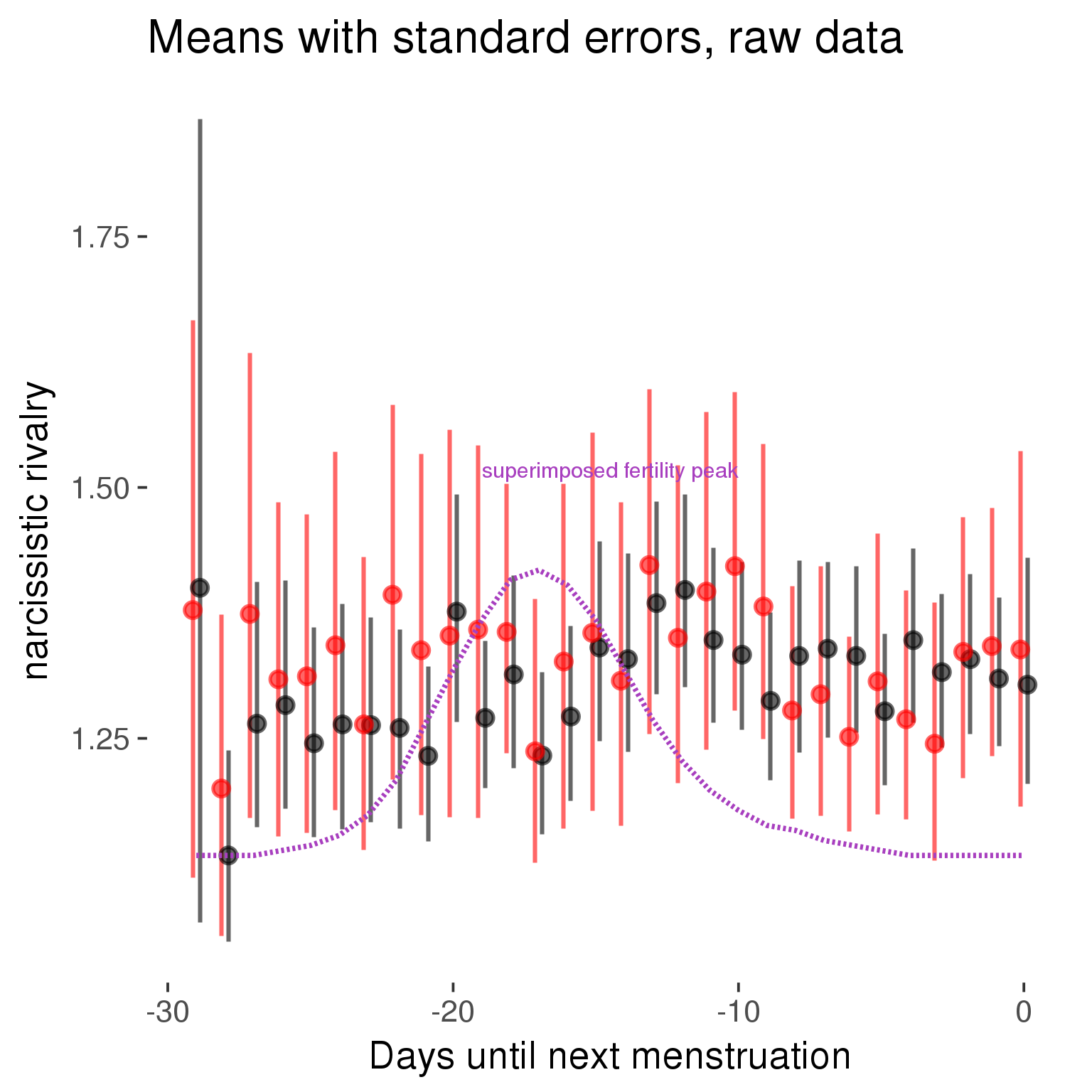
Forward-counted
model %>%
plot_curve(diary %>% filter(minimum_cycle_length_diary <= 30, minimum_cycle_length_diary >= 27) %>% mutate(RCD = FCD, fertile = prc_stirn_b_forward_counted), caption_x = "Days since last menstruation")outcome = names(model@frame)[1]
outcome_label = recode(str_replace_all(str_replace_all(str_replace_all(outcome, "_", " "), " pair", "-pair"), " 1", ""),
"desirability 1" = "self-perceived desirability",
"NARQ admiration" = "narcissistic admiration",
"NARQ rivalry" = "narcissistic rivalry",
"extra-pair" = "extra-pair desire & behaviour",
"had sexual intercourse" = "sexual intercourse")
library(ggplot2)
# form a subset and run the model without the hormonal contraception and the fertility predictors
tmp = diary %>%
filter(!is.na(fertile), !is.na(included),
RCD > -1 * minimum_cycle_length_diary, RCD > -40)
new_form = update.formula(formula(model), new = . ~ . - fertile * included)
tmp$residuals = residuals(update(model, new_form, data = tmp , na.action = na.exclude))
tmp = tmp %>%
filter(!is.na(RCD), !is.na(residuals))
rcd_min = min(tmp$RCD)
tmp$real = FALSE
tmp_before = tmp
tmp_before$RCD = tmp_before$RCD + min(tmp$RCD) - 1
tmp_after = tmp
tmp_after$RCD = tmp_after$RCD - min(tmp$RCD) + 1
tmp$real = TRUE
tmp = bind_rows(tmp_before %>% filter(RCD > rcd_min - 11), tmp, tmp_after %>% filter(RCD < 11))GAM smooth on residuals
Here, we partialled out menstruation and individual random effects, then superimposed estimated probability of being in the fertile window scaled to the range of the estimated means. To address the periodicity of the cycle, we prepended and appended ten days of the timeseries to the end and the beginning of the timeseries. We then estimated the GAM and cut off the appended subsets before plotting.
tryCatch({
trend_plot = ggplot(tmp,aes(x = RCD, y = residuals, colour = included)) +
stat_smooth(geom = 'smooth',size = 0.8, fill = "#9ECAE1", method = 'gam', formula = y ~ s(x))
}, error = function(e){cat_message(e, "danger")})
tryCatch({
trend_data = ggplot_build(trend_plot)$data[[1]]
}, error = function(e){cat_message(e, "danger")})
trend_data$RCD = round(trend_data$x)
trend_data = left_join(trend_data, tmp %>% select(real, RCD,fertile) %>% unique(), by = "RCD")
trend_data %>%
filter(real == TRUE) %>%
mutate(superimposed = ( ( (fertile - 0.01)/0.58) * (max(y)-min(y) ) ) + min(y) ) ->
trend_data
ggplot(trend_data) +
geom_ribbon(aes(x = x, ymin = ymin, ymax = ymax, fill = factor(group)), alpha = 0.2) +
geom_line(aes(x = x, y = y, colour = factor(group)), size = 0.8, stat = "identity") +
scale_x_continuous(caption_x) +
geom_line(aes(x = x, y = superimposed), color = "#a83fbf", size = 1, linetype = 'dashed') +
annotate("text",x = mean(trend_data$x), y = max(trend_data$superimposed,na.rm=T) + 0.1, label = 'superimposed fertility peak', color = "#a83fbf") +
scale_y_continuous(outcome_label) +
ggtitle("GAM smooth, residuals") +
scale_color_manual("Contraception status",values = c("2"="black","1"= "red"), labels = c("2"="hormonally\ncontracepting","1"="cycling"), guide = F) +
scale_fill_manual("Contraception status",values = c("2"="black","1"= "red"), labels = c("2"="hormonally\ncontracepting","1"="cycling"), guide = F)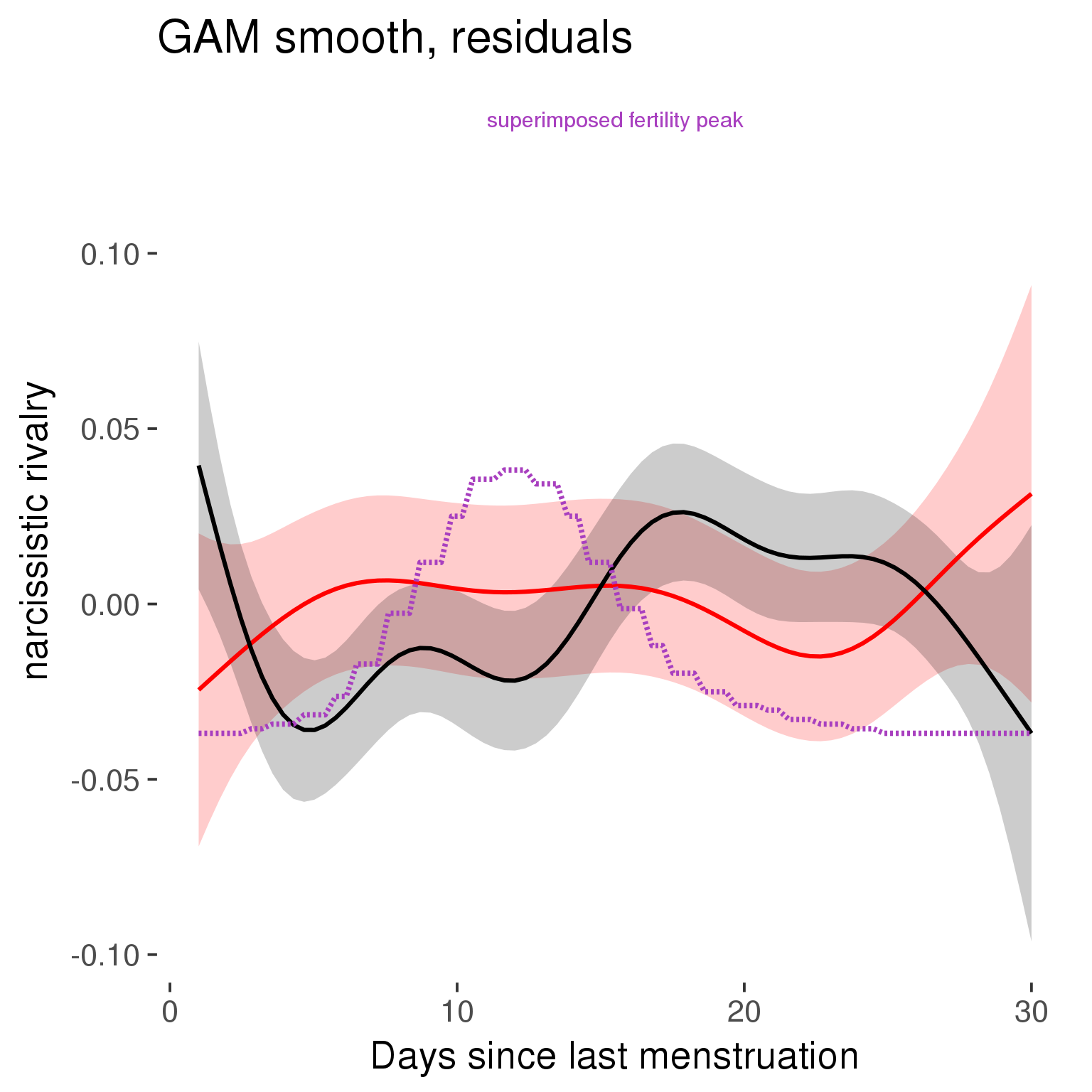
GAM smooth on raw data
As before, but without partialling anything out.
tryCatch({
trend_plot = ggplot(tmp,aes_string(x = "RCD", y = outcome, colour = "included")) +
stat_smooth(geom = 'smooth',size = 0.8, fill = "#9ECAE1", method = 'gam', formula = y ~ s(x))
}, error = function(e){cat_message(e, "danger")})
tryCatch({
trend_data = ggplot_build(trend_plot)$data[[1]]
}, error = function(e){cat_message(e, "danger")})
trend_data$RCD = round(trend_data$x)
trend_data = left_join(trend_data, tmp %>% select(real, RCD,fertile) %>% unique(), by = "RCD")
trend_data %>%
filter(real == TRUE) %>%
mutate(superimposed = ( ( (fertile - 0.01)/0.58) * (max(y)-min(y) ) ) + min(y) ) ->
trend_data
plot1b = ggplot(trend_data) +
geom_ribbon(aes(x = x, ymin = ymin, ymax = ymax, fill = factor(group)), alpha = 0.2) +
geom_line(aes(x = x, y = y, colour = factor(group)), size = 0.8, stat = "identity") +
scale_x_continuous(caption_x) +
geom_line(aes(x = x, y = superimposed), color = "#a83fbf", size = 1, linetype = 'dashed') +
annotate("text",x = mean(trend_data$x), y = max(trend_data$superimposed,na.rm=T) + 0.1, label = 'superimposed fertility peak', color = "#a83fbf") +
scale_y_continuous(outcome_label) +
ggtitle("GAM smooth, raw data") +
scale_color_manual("Contraception status",values = c("2"="black","1"= "red"), labels = c("2"="hormonally\ncontracepting","1"="cycling"), guide = F) +
scale_fill_manual("Contraception status",values = c("2"="black","1"= "red"), labels = c("2"="hormonally\ncontracepting","1"="cycling"), guide = F)
suppressWarnings(print(plot1b))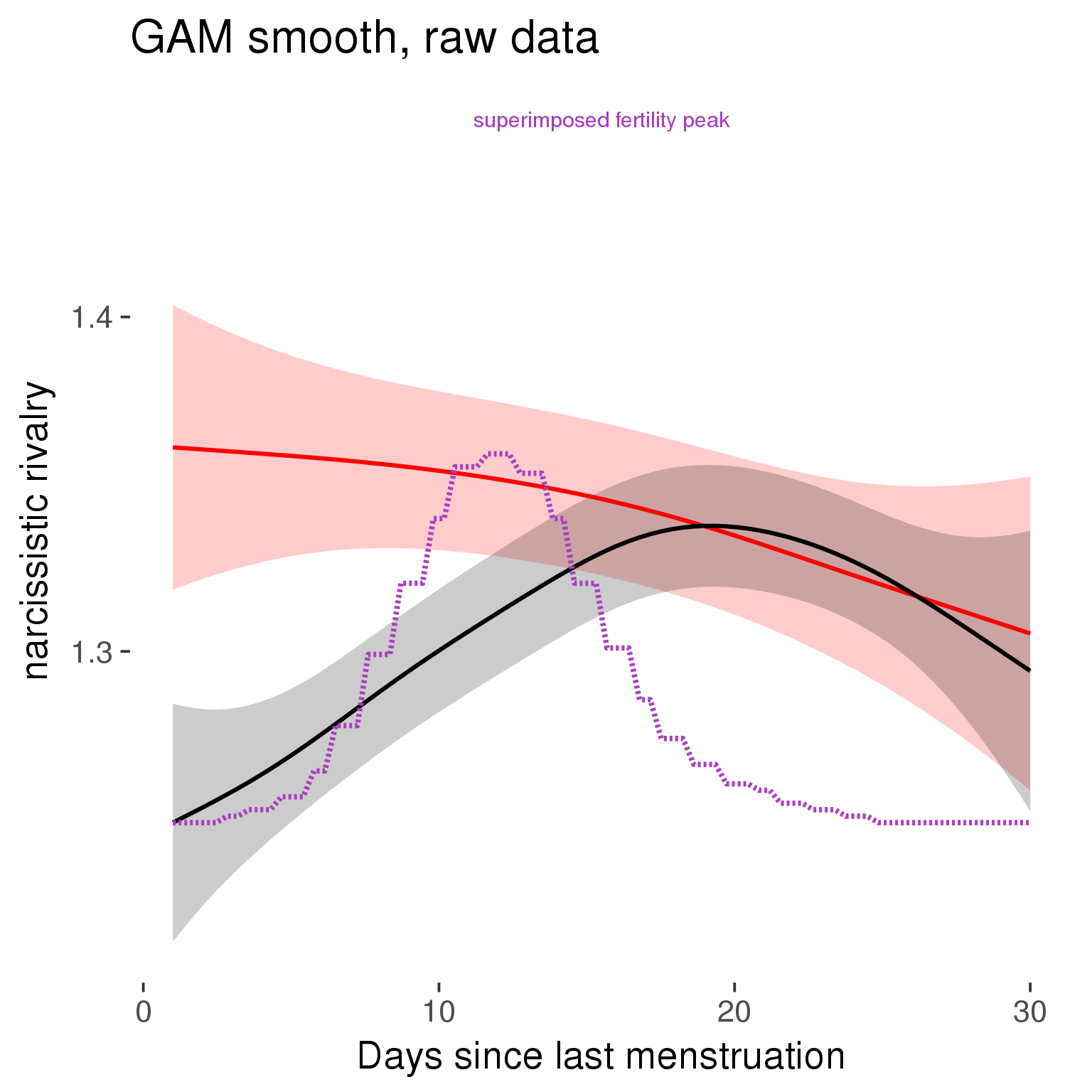
Means and standard errors over raw data
Nothing partialled out, just straight means with bootstrapped confidence intervals.
tryCatch({
trend_plot = ggplot(tmp,aes_string(x = "RCD", y = outcome, colour = "included")) +
geom_pointrange(size = 0.8, stat = 'summary', fun.data = "mean_cl_boot")
}, error = function(e){cat_message(e, "danger")})
tryCatch({
trend_data = ggplot_build(trend_plot)$data[[1]]
}, error = function(e){cat_message(e, "danger")})
trend_data$RCD = round(trend_data$x)
trend_data = left_join(trend_data, tmp %>% select(real, RCD,fertile) %>% unique(), by = "RCD")
trend_data %>%
filter(real == TRUE) %>%
mutate(superimposed = ( ( (fertile - 0.01)/0.58) * (max(y)-min(y) ) ) + min(y) ) ->
trend_data
plot3 = ggplot(trend_data) +
geom_pointrange(aes(x = x, y = y, ymin = ymin,ymax = ymax, colour = factor(group)), size = 0.8, stat = "identity", alpha = 0.6, position = position_dodge(width = .5)) +
scale_x_continuous("Days until next menstruation") +
geom_line(aes(x= x, y = superimposed), color = "#a83fbf", size = 1, linetype = 'dashed') +
annotate("text",x = mean(trend_data$x), y = max(trend_data$superimposed,na.rm=T) + 0.1, label = 'superimposed fertility peak', color = "#a83fbf") +
scale_y_continuous(outcome_label) +
ggtitle("Means with standard errors, raw data") +
scale_color_manual("Contraception status",values = c("2"="black","1"= "red"), labels = c("2"="hormonally\ncontracepting","1"="cycling"), guide = F) +
scale_fill_manual("Contraception status",values = c("2"="black","1"= "red"), labels = c("2"="hormonally\ncontracepting","1"="cycling"), guide = F)
suppressWarnings(print(plot3))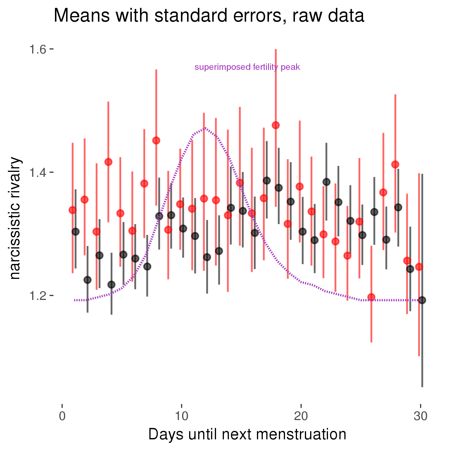
Robustness checks
M_r1: Random slopes for conception risk and menstruation
tryCatch({
# refit model with random effects for fertile and menstruation dummies
with_ind_diff = update(model, formula = . ~ . - (1| person) + (1 + fertile + menstruation | person))
# pull the random effects, format as tibble
rand = coef(with_ind_diff)$person %>%
tibble::rownames_to_column("person") %>%
mutate(person = as.numeric(person))
# pull the fixed effects
fixd = data.frame(fixef(with_ind_diff)) %>%
tibble::rownames_to_column("effect")
names(fixd) = c("effect", "pop_effect_size")
# pull apart the coefficients so that we can account for the fact that the random effect variation implicitly includes HC explaining the mean population-level effect of fertile/menstruation dummies among HC users
fixd = fixd %>%
separate(effect, c("included", "effect"), sep = ":", fill = "left") %>%
mutate(included = if_else(is.na(included), "cycling", str_replace(included, "included", "")))
fixd[2,c("included", "effect")] = c("horm_contra", "(Intercept)")
rand = rand %>%
# merge diary data on the random effects, so that we know who is a HC users and who isn't
inner_join(diary %>% select(person, included) %>% unique(), by = 'person') %>%
# gather into long format, to have the dataset by predictor
gather(effect, value, -person, -included) %>%
inner_join(fixd, by = c('effect', 'included')) %>%
# pull the fixed effects
mutate(
# only for those who are HC users, add the moderated population effect size for this effect (the random effects have the reference category mean)
value = if_else(included == "horm_contra", value + pop_effect_size, value),
effect = recode(effect, "includedhorm_contra" = "HC user",
"includedhorm_contra:fertile" = "HC user x fertile",
"includedhorm_contra:menstruationpre" = "HC user x premens.",
"includedhorm_contra:menstruationyes" = "HC user x mens.",
"menstruationyes" = "mens.",
"menstruationpre" = "premens.")) %>%
group_by(included, effect) %>%
# filter out predictors that aren't modelled as varying/random
filter(sd(value) > 0)
# plot dot plot of random effects
print(
ggplot(rand, aes(x = included, y = value, color = included, fill = included)) +
facet_wrap( ~ effect, scales = "free") +
# geom_violin(alpha = 0.4, size = 0) +
geom_dotplot(binaxis='y', dotsize = 0.1, method = "histodot") +
# geom_jitter(alpha = 0.05) +
coord_flip() +
geom_pointrange(stat = 'summary', fun.data = 'mean_sdl', color = 'darkred', size = 1.2) +
scale_color_manual("Contraception status", values = c("horm_contra"="black","cycling"= "red"), labels = c("horm_contra"="hormonally\ncontracepting","cycling"="cycling"), guide = F) +
scale_fill_manual("Contraception status", values = c("horm_contra"="black","cycling"= "red"), labels = c("horm_contra"="hormonally\ncontracepting","1"="cycling"), guide = F) +
ggtitle("M_r1: allowing participant-varying slopes", subtitle = "for the conception risk measure and the menstruation dummies") +
scale_x_discrete("Hormonal contraception", breaks = c("horm_contra", "cycling"), labels = c("yes", "no")) +
scale_y_continuous("Random effect size distribution"))
print_summary(with_ind_diff)
cat(pander(anova(model, with_ind_diff)))
}, error = function(e){
with_ind_diff = model
cat_message(e, "danger")
})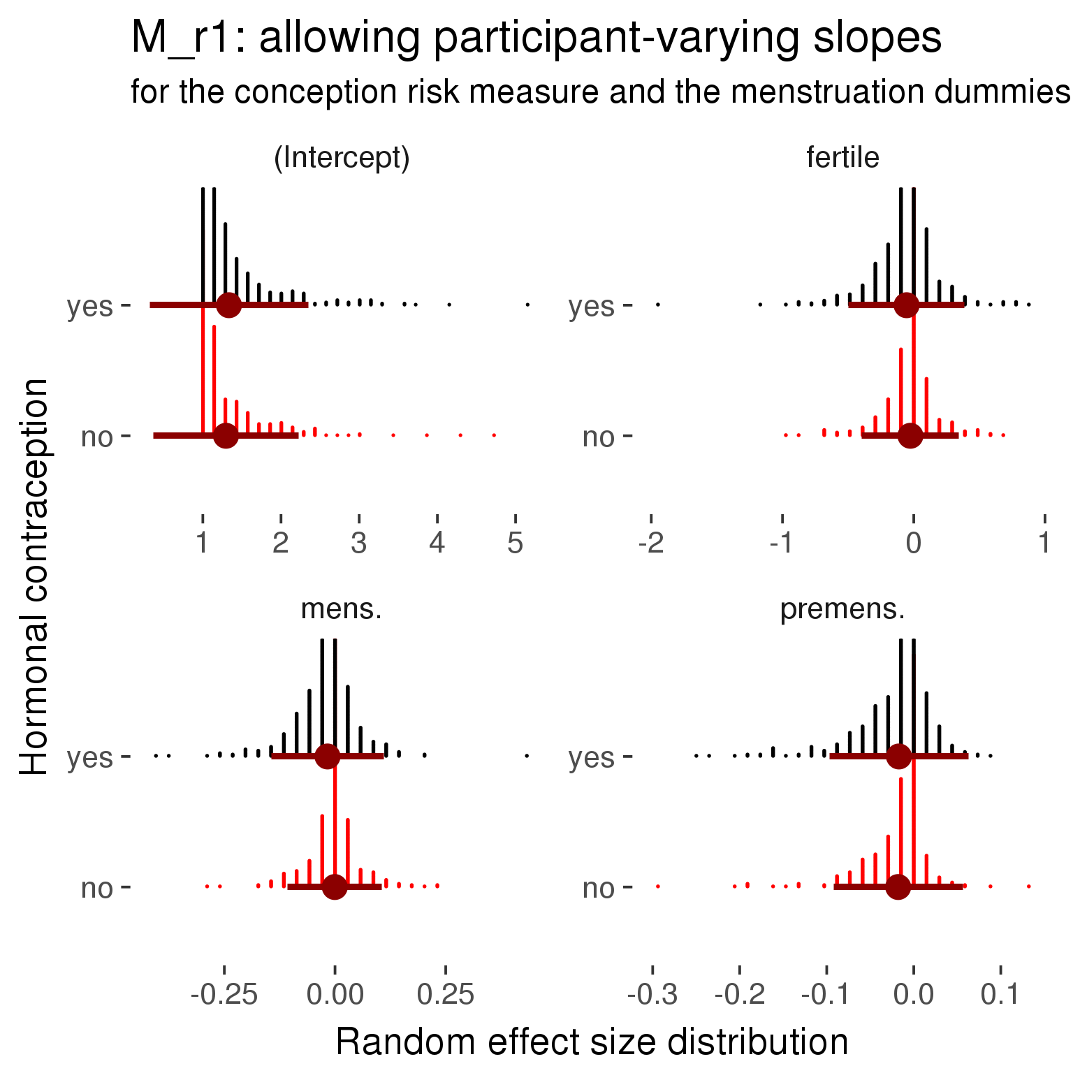
Linear mixed model fit by REML ['lmerMod']
Formula: NARQ_rivalry ~ included + menstruation + fertile + fertile_mean +
(1 + fertile + menstruation | person) + included:menstruation + included:fertile
Data: diary
REML criterion at convergence: 41710
Scaled residuals:
Min 1Q Median 3Q Max
-5.110 -0.321 -0.084 -0.016 9.708
Random effects:
Groups Name Variance Std.Dev. Corr
person (Intercept) 0.26766 0.5174
fertile 0.13340 0.3652 -0.31
menstruationpre 0.00686 0.0829 -0.34 -0.22
menstruationyes 0.01891 0.1375 -0.25 0.37 0.31
Residual 0.24160 0.4915
Number of obs: 26681, groups: person, 1054
Fixed effects:
Estimate Std. Error t value
(Intercept) 1.295998 0.042179 30.73
includedhorm_contra 0.038347 0.035579 1.08
menstruationpre -0.017898 0.015930 -1.12
menstruationyes -0.000585 0.016309 -0.04
fertile -0.025493 0.036921 -0.69
fertile_mean 0.080794 0.189150 0.43
includedhorm_contra:menstruationpre 0.000882 0.020449 0.04
includedhorm_contra:menstruationyes -0.016394 0.021281 -0.77
includedhorm_contra:fertile -0.029095 0.046873 -0.62
Correlation of Fixed Effects:
(Intr) incld_ mnstrtnp mnstrtny fertil frtl_m inclddhrm_cntr:mnstrtnp
inclddhrm_c -0.489
menstrutnpr -0.192 0.224
menstrutnys -0.189 0.227 0.374
fertile -0.197 0.298 0.334 0.376
fertile_men -0.757 -0.024 0.004 -0.004 -0.071
inclddhrm_cntr:mnstrtnp 0.153 -0.284 -0.779 -0.292 -0.260 -0.007
inclddhrm_cntr:mnstrtny 0.150 -0.283 -0.287 -0.766 -0.288 -0.004 0.363
inclddhrm_cntr:f 0.189 -0.380 -0.263 -0.296 -0.784 0.010 0.333
inclddhrm_cntr:mnstrtny
inclddhrm_c
menstrutnpr
menstrutnys
fertile
fertile_men
inclddhrm_cntr:mnstrtnp
inclddhrm_cntr:mnstrtny
inclddhrm_cntr:f 0.372
refitting model(s) with ML (instead of REML)
| Df | AIC | BIC | logLik | deviance | Chisq | Chi Df | Pr(>Chisq) | |
|---|---|---|---|---|---|---|---|---|
| object | 11 | 41836 | 41926 | -20907 | 41814 | NA | NA | NA |
| ..1 | 20 | 41700 | 41864 | -20830 | 41660 | 154.6 | 9 | 9.821e-29 |
robustness_check_ovu_shift(model, diary)M_e: Exclusion criteria
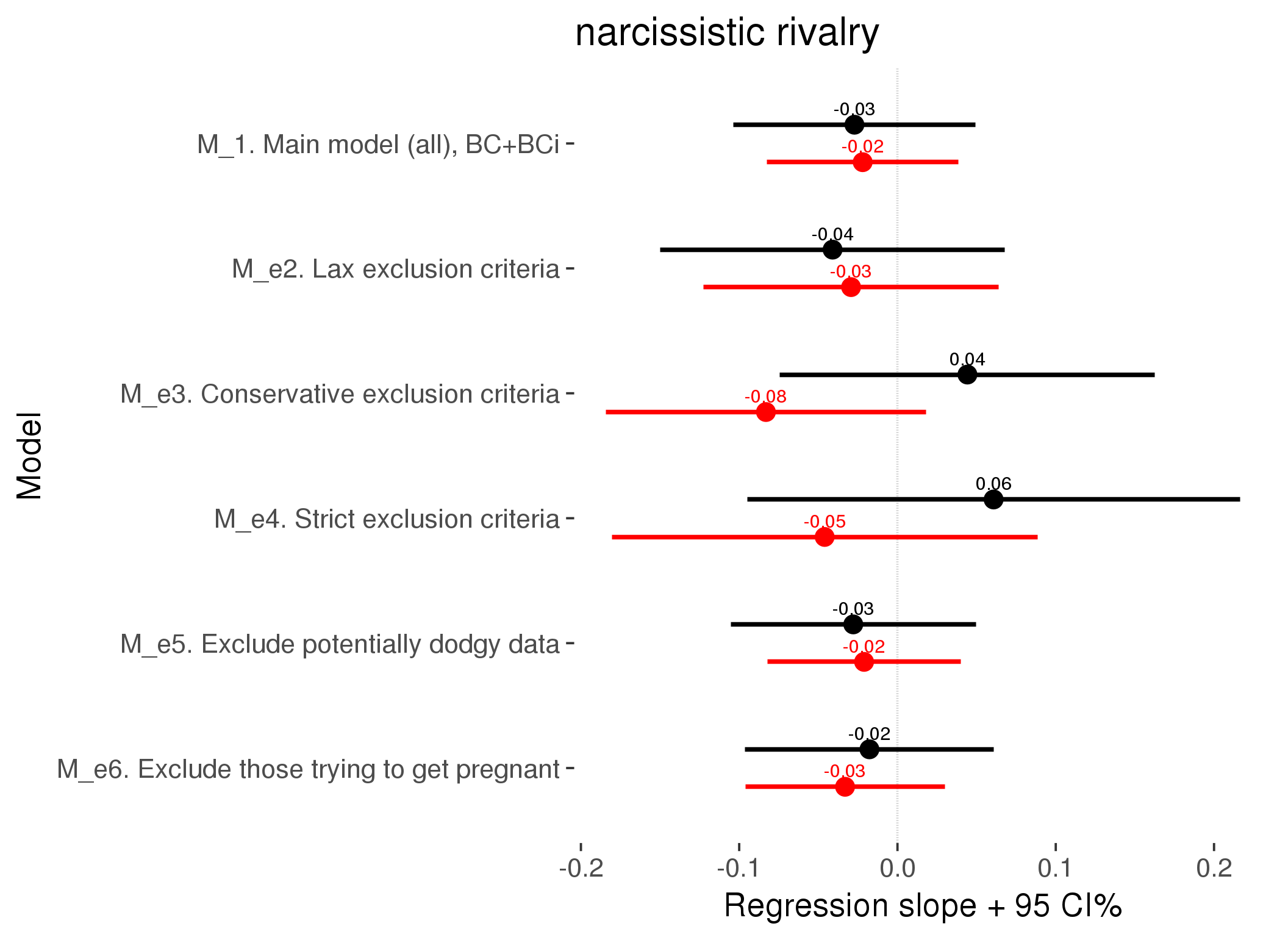
M_p: Predictors

M_c: Covariates, controls, autocorrelation
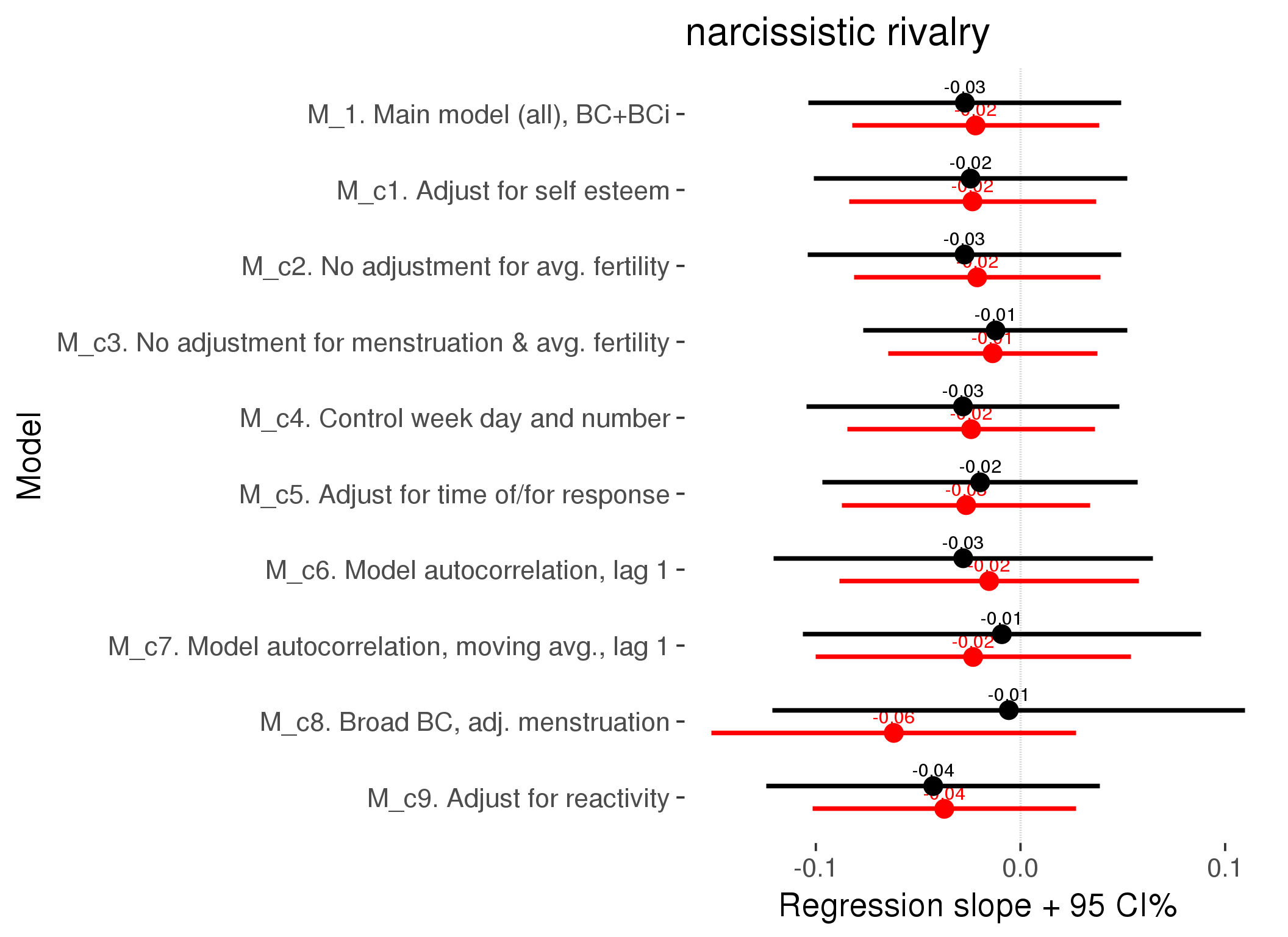
Linear mixed model fit by REML ['lmerMod']
REML criterion at convergence: 38399
Scaled residuals:
Min 1Q Median 3Q Max
-4.982 -0.330 -0.099 0.005 9.689
Random effects:
Groups Name Variance Std.Dev.
person (Intercept) 0.23909 0.4890
Xr.2 s(days_filled_out):includedhorm_contra 0.06267 0.2503
Xr.1 s(days_filled_out):includedcycling 0.03122 0.1767
Xr.0 s(day_number):includedhorm_contra 0.00742 0.0861
Xr s(day_number):includedcycling 0.00000 0.0000
Residual 0.24865 0.4987
Number of obs: 24379, groups: person, 1054; Xr.2, 8; Xr.1, 8; Xr.0, 8; Xr, 8
Fixed effects:
Estimate Std. Error t value
X(Intercept) 1.282059 0.041447 30.93
Xincludedhorm_contra 0.046480 0.034268 1.36
Xmenstruationpre -0.020452 0.015939 -1.28
Xmenstruationyes -0.005607 0.015310 -0.37
Xfertile -0.037242 0.032819 -1.13
Xfertile_mean 0.111776 0.188155 0.59
Xincludedhorm_contra:menstruationpre -0.000676 0.020446 -0.03
Xincludedhorm_contra:menstruationyes -0.012575 0.020039 -0.63
Xincludedhorm_contra:fertile -0.042641 0.041577 -1.03
Xs(day_number):includedcyclingFx1 0.066268 0.026515 2.50
Xs(day_number):includedhorm_contraFx1 0.026940 0.042184 0.64
Xs(days_filled_out):includedcyclingFx1 -0.149026 0.051341 -2.90
Xs(days_filled_out):includedhorm_contraFx1 -0.136404 0.061205 -2.23
Family: gaussian
Link function: identity
Formula:
NARQ_rivalry ~ included + menstruation + fertile + fertile_mean +
s(day_number, by = included) + s(days_filled_out, by = included) +
included:menstruation + included:fertile
Parametric coefficients:
Estimate Std. Error t value Pr(>|t|)
(Intercept) 1.282059 0.041447 30.93 <2e-16 ***
includedhorm_contra 0.046480 0.034268 1.36 0.17
menstruationpre -0.020452 0.015939 -1.28 0.20
menstruationyes -0.005607 0.015310 -0.37 0.71
fertile -0.037242 0.032819 -1.13 0.26
fertile_mean 0.111776 0.188155 0.59 0.55
includedhorm_contra:menstruationpre -0.000676 0.020446 -0.03 0.97
includedhorm_contra:menstruationyes -0.012575 0.020039 -0.63 0.53
includedhorm_contra:fertile -0.042641 0.041577 -1.03 0.31
---
Signif. codes: 0 '***' 0.001 '**' 0.01 '*' 0.05 '.' 0.1 ' ' 1
Approximate significance of smooth terms:
edf Ref.df F p-value
s(day_number):includedcycling 1.00 1.00 6.25 0.0125 *
s(day_number):includedhorm_contra 2.52 2.52 1.56 0.1860
s(days_filled_out):includedcycling 4.32 4.32 2.99 0.0097 **
s(days_filled_out):includedhorm_contra 5.40 5.40 3.06 0.0056 **
---
Signif. codes: 0 '***' 0.001 '**' 0.01 '*' 0.05 '.' 0.1 ' ' 1
R-sq.(adj) = 0.00267
lmer.REML = 38399 Scale est. = 0.24865 n = 24379
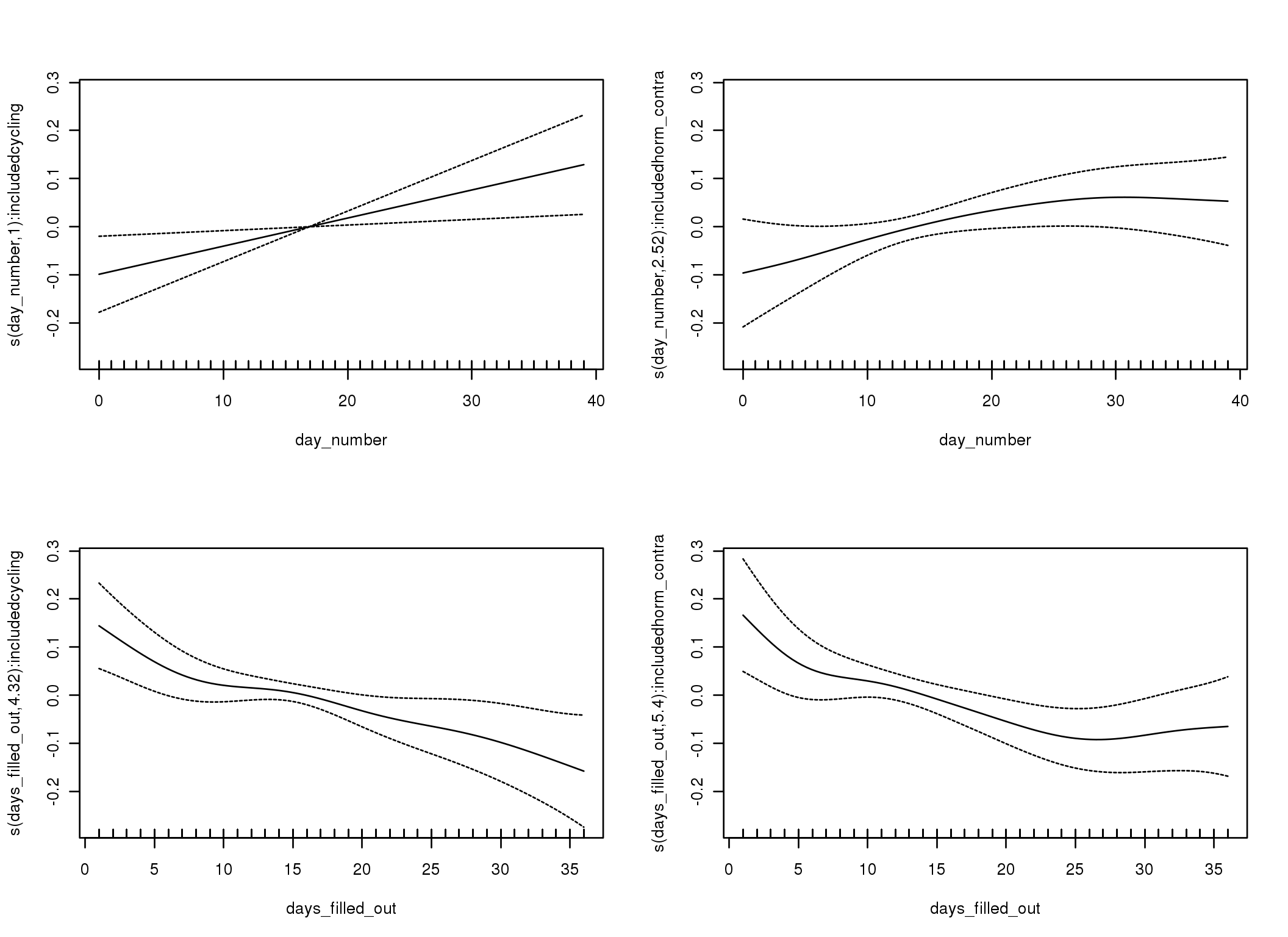
Linear mixed-effects model fit by REML
Data: diary
AIC BIC logLik
40486 40584 -20231
Random effects:
Formula: ~1 | person
(Intercept) Residual
StdDev: 0.4848 0.5068
Correlation Structure: ARMA(1,0)
Formula: ~day_number | person
Parameter estimate(s):
Phi1
0.2817
Fixed effects: NARQ_rivalry ~ included * (menstruation + fertile) + fertile_mean
Value Std.Error DF t-value p-value
(Intercept) 1.2935 0.04197 25621 30.821 0.0000
includedhorm_contra 0.0372 0.03459 1051 1.076 0.2820
menstruationpre -0.0140 0.01762 25621 -0.793 0.4276
menstruationyes -0.0001 0.01646 25621 -0.009 0.9931
fertile -0.0153 0.03732 25621 -0.411 0.6811
fertile_mean 0.0881 0.19153 1051 0.460 0.6457
includedhorm_contra:menstruationpre 0.0017 0.02263 25621 0.076 0.9391
includedhorm_contra:menstruationyes -0.0064 0.02146 25621 -0.299 0.7648
includedhorm_contra:fertile -0.0280 0.04723 25621 -0.593 0.5534
Correlation:
(Intr) incld_ mnstrtnp mnstrtny fertil frtl_m inclddhrm_cntr:mnstrtnp
includedhorm_contra -0.477
menstruationpre -0.159 0.200
menstruationyes -0.156 0.195 0.403
fertile -0.153 0.254 0.430 0.362
fertile_mean -0.769 -0.024 -0.008 -0.006 -0.072
includedhorm_contra:menstruationpre 0.131 -0.250 -0.779 -0.313 -0.334 -0.003
includedhorm_contra:menstruationyes 0.125 -0.238 -0.309 -0.767 -0.278 -0.003 0.388
includedhorm_contra:fertile 0.155 -0.321 -0.339 -0.286 -0.787 0.013 0.429
inclddhrm_cntr:mnstrtny
includedhorm_contra
menstruationpre
menstruationyes
fertile
fertile_mean
includedhorm_contra:menstruationpre
includedhorm_contra:menstruationyes
includedhorm_contra:fertile 0.357
Standardized Within-Group Residuals:
Min Q1 Med Q3 Max
-4.79292 -0.33854 -0.10200 -0.02584 9.50011
Number of Observations: 26681
Number of Groups: 1054
Linear mixed-effects model fit by REML
Data: diary
AIC BIC logLik
39998 40105 -19986
Random effects:
Formula: ~1 | person
(Intercept) Residual
StdDev: 0.4666 0.52
Correlation Structure: ARMA(1,1)
Formula: ~day_number | person
Parameter estimate(s):
Phi1 Theta1
0.8123 -0.5906
Fixed effects: NARQ_rivalry ~ included * (menstruation + fertile) + fertile_mean
Value Std.Error DF t-value p-value
(Intercept) 1.3009 0.04192 25621 31.035 0.0000
includedhorm_contra 0.0311 0.03445 1051 0.902 0.3674
menstruationpre -0.0189 0.01745 25621 -1.081 0.2795
menstruationyes -0.0041 0.01675 25621 -0.244 0.8073
fertile -0.0232 0.03928 25621 -0.589 0.5555
fertile_mean 0.0676 0.19210 1051 0.352 0.7252
includedhorm_contra:menstruationpre 0.0048 0.02244 25621 0.214 0.8304
includedhorm_contra:menstruationyes 0.0009 0.02174 25621 0.041 0.9672
includedhorm_contra:fertile -0.0091 0.04960 25621 -0.184 0.8544
Correlation:
(Intr) incld_ mnstrtnp mnstrtny fertil frtl_m inclddhrm_cntr:mnstrtnp
includedhorm_contra -0.474
menstruationpre -0.154 0.190
menstruationyes -0.159 0.198 0.442
fertile -0.148 0.255 0.343 0.337
fertile_mean -0.770 -0.027 -0.002 -0.004 -0.078
includedhorm_contra:menstruationpre 0.124 -0.236 -0.778 -0.344 -0.266 -0.003
includedhorm_contra:menstruationyes 0.127 -0.242 -0.340 -0.770 -0.259 -0.002 0.431
includedhorm_contra:fertile 0.153 -0.322 -0.271 -0.267 -0.788 0.014 0.341
inclddhrm_cntr:mnstrtny
includedhorm_contra
menstruationpre
menstruationyes
fertile
fertile_mean
includedhorm_contra:menstruationpre
includedhorm_contra:menstruationyes
includedhorm_contra:fertile 0.332
Standardized Within-Group Residuals:
Min Q1 Med Q3 Max
-4.3593 -0.3466 -0.1278 -0.0553 9.2983
Number of Observations: 26681
Number of Groups: 1054
M_d: Other designs
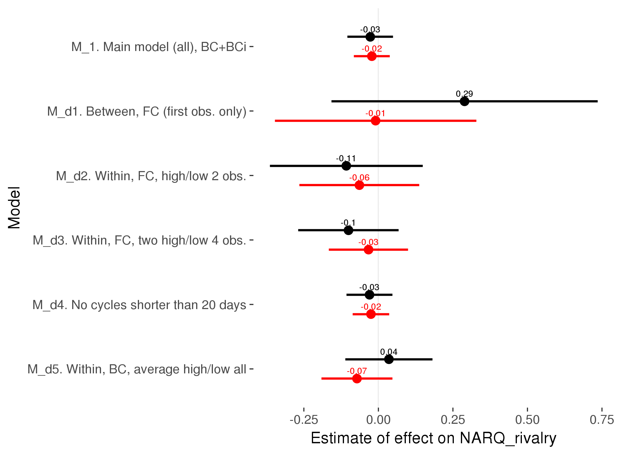
M_m1: Moderation by contraceptive method
Based on the sample with lax exclusion criteria. Users who used any hormonal contraception are classified as hormonal, users who use any awareness-based methods (counting, temperature-based) are classified as ‘fertility-awareness’, women who don’t fall into the before groups and use condoms, pessars, coitus interruptus etc. are classified as ‘barrie or abstinence’. Women who don’t use contraception or use other methods such as sterilisation are excluded from this analysis.
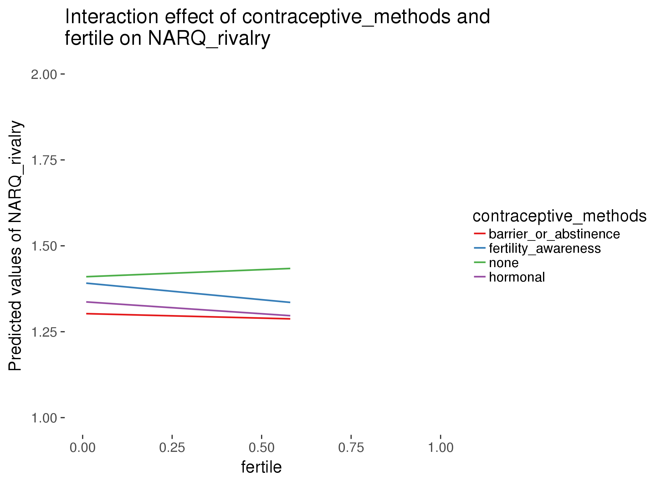
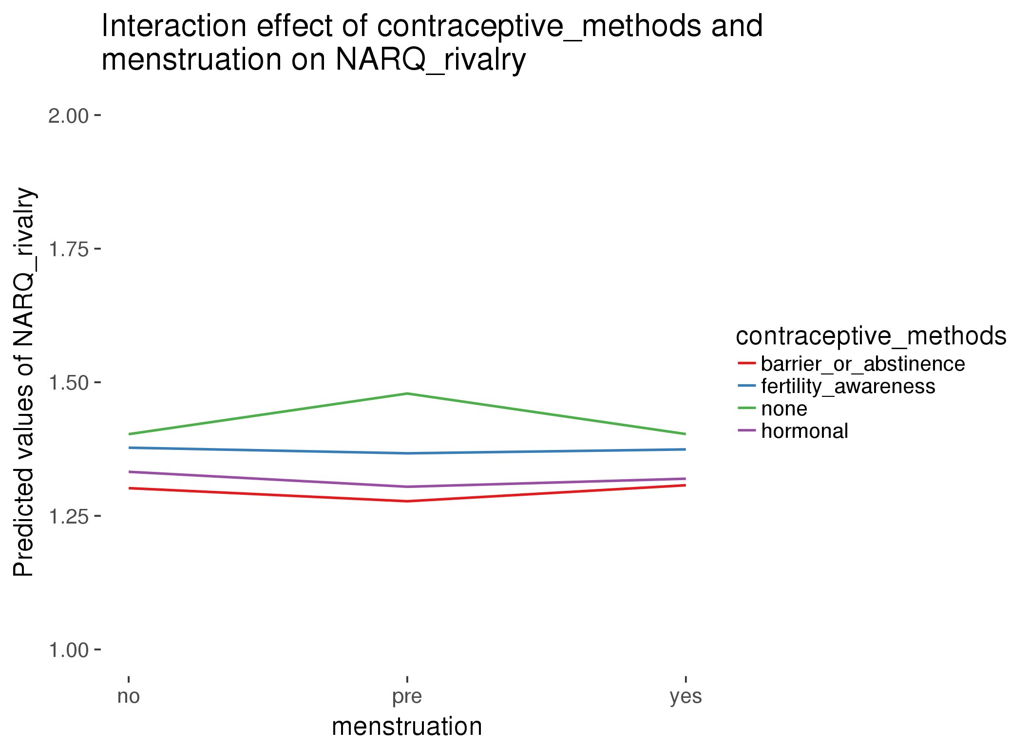
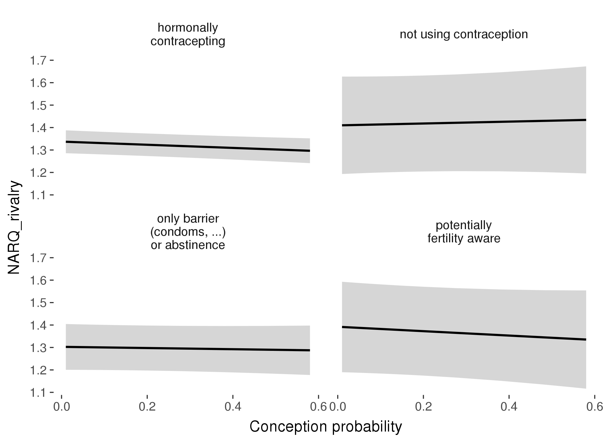
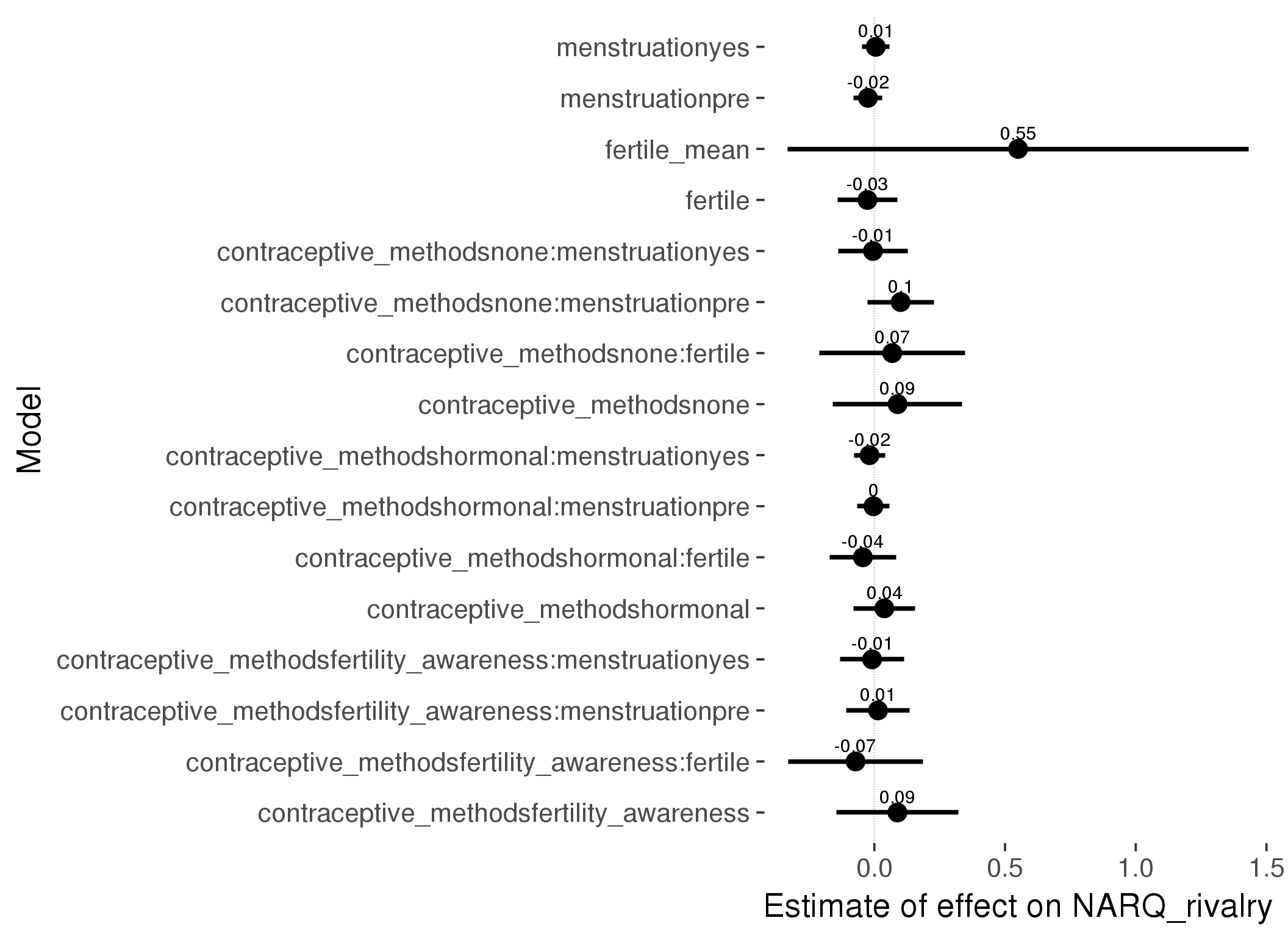
Linear mixed model fit by REML ['lmerMod']
Formula: NARQ_rivalry ~ fertile_mean + (1 | person) + contraceptive_methods +
fertile + menstruation + fertile:contraceptive_methods + menstruation:contraceptive_methods
Data: diary
Subset: !is.na(included_lax) & contraceptive_method != "other"
REML criterion at convergence: 27783
Scaled residuals:
Min 1Q Median 3Q Max
-4.774 -0.336 -0.094 -0.003 9.307
Random effects:
Groups Name Variance Std.Dev.
person (Intercept) 0.236 0.486
Residual 0.270 0.519
Number of obs: 17027, groups: person, 513
Fixed effects:
Estimate Std. Error t value
(Intercept) 1.21001 0.09234 13.10
fertile_mean 0.55005 0.45010 1.22
contraceptive_methodsfertility_awareness 0.08830 0.11900 0.74
contraceptive_methodsnone 0.08904 0.12608 0.71
contraceptive_methodshormonal 0.03830 0.06004 0.64
fertile -0.02645 0.05794 -0.46
menstruationpre -0.02450 0.02798 -0.88
menstruationyes 0.00544 0.02674 0.20
contraceptive_methodsfertility_awareness:fertile -0.07178 0.13157 -0.55
contraceptive_methodsnone:fertile 0.06845 0.14243 0.48
contraceptive_methodshormonal:fertile -0.04386 0.06473 -0.68
contraceptive_methodsfertility_awareness:menstruationpre 0.01400 0.06197 0.23
contraceptive_methodsnone:menstruationpre 0.10055 0.06480 1.55
contraceptive_methodshormonal:menstruationpre -0.00346 0.03152 -0.11
contraceptive_methodsfertility_awareness:menstruationyes -0.00862 0.06229 -0.14
contraceptive_methodsnone:menstruationyes -0.00526 0.06776 -0.08
contraceptive_methodshormonal:menstruationyes -0.01836 0.03050 -0.60
refitting model(s) with ML (instead of REML)
| Df | AIC | BIC | logLik | deviance | Chisq | Chi Df | Pr(>Chisq) | |
|---|---|---|---|---|---|---|---|---|
| add_main | 13 | 27742 | 27843 | -13858 | 27716 | NA | NA | NA |
| by_method | 19 | 27751 | 27898 | -13856 | 27713 | 3.534 | 6 | 0.7395 |
M_m2: Moderation by participant age
model %>%
test_moderator("age_group", diary, xlevels = 5)refitting model(s) with ML (instead of REML)
| Df | AIC | BIC | logLik | deviance | Chisq | Chi Df | Pr(>Chisq) | |
|---|---|---|---|---|---|---|---|---|
| with_main | 19 | 41840 | 41996 | -20901 | 41802 | NA | NA | NA |
| with_mod | 27 | 41849 | 42071 | -20898 | 41795 | 6.927 | 8 | 0.5446 |
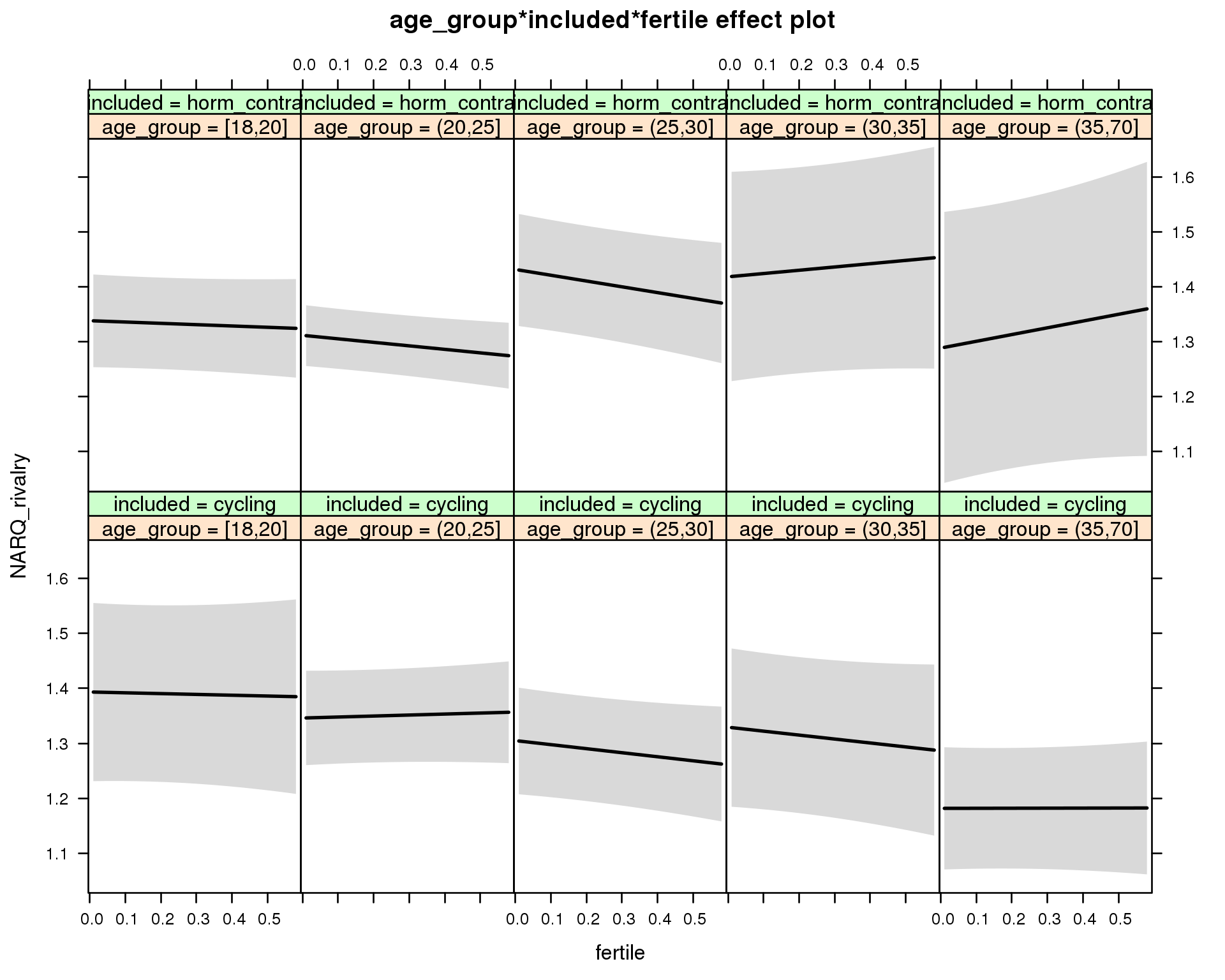
Linear mixed model fit by REML ['lmerMod']
Formula: NARQ_rivalry ~ menstruation + fertile_mean + (1 | person) + age_group +
included + fertile + menstruation:included + age_group:included +
age_group:fertile + included:fertile + age_group:included:fertile
Data: diary
REML criterion at convergence: 41900
Scaled residuals:
Min 1Q Median 3Q Max
-4.983 -0.328 -0.090 -0.011 9.681
Random effects:
Groups Name Variance Std.Dev.
person (Intercept) 0.239 0.489
Residual 0.249 0.499
Number of obs: 26681, groups: person, 1054
Fixed effects:
Estimate Std. Error t value
(Intercept) 1.385376 0.087231 15.88
menstruationpre -0.018279 0.015266 -1.20
menstruationyes 0.003676 0.014399 0.26
fertile_mean 0.061702 0.188708 0.33
age_group(20,25] -0.047347 0.093691 -0.51
age_group(25,30] -0.088430 0.096422 -0.92
age_group(30,35] -0.064092 0.110664 -0.58
age_group(35,70] -0.211692 0.100226 -2.11
includedhorm_contra -0.052043 0.093782 -0.55
fertile -0.014671 0.088079 -0.17
menstruationpre:includedhorm_contra 0.000528 0.019600 0.03
menstruationyes:includedhorm_contra -0.019642 0.018872 -1.04
age_group(20,25]:includedhorm_contra 0.020751 0.106935 0.19
age_group(25,30]:includedhorm_contra 0.181669 0.117704 1.54
age_group(30,35]:includedhorm_contra 0.143940 0.153431 0.94
age_group(35,70]:includedhorm_contra 0.161951 0.166716 0.97
age_group(20,25]:fertile 0.032709 0.097584 0.34
age_group(25,30]:fertile -0.058768 0.100579 -0.58
age_group(30,35]:fertile -0.057039 0.116511 -0.49
age_group(35,70]:fertile 0.015839 0.105122 0.15
includedhorm_contra:fertile -0.009305 0.097688 -0.10
age_group(20,25]:includedhorm_contra:fertile -0.072553 0.109307 -0.66
age_group(25,30]:includedhorm_contra:fertile -0.022567 0.121134 -0.19
age_group(30,35]:includedhorm_contra:fertile 0.140706 0.156361 0.90
age_group(35,70]:includedhorm_contra:fertile 0.130934 0.177596 0.74
M_m3: Moderation by weekend
model %>%
test_moderator("weekend", diary, xlevels = 2) refitting model(s) with ML (instead of REML)
| Df | AIC | BIC | logLik | deviance | Chisq | Chi Df | Pr(>Chisq) | |
|---|---|---|---|---|---|---|---|---|
| with_main | 13 | 41839 | 41946 | -20907 | 41813 | NA | NA | NA |
| with_mod | 15 | 41843 | 41966 | -20907 | 41813 | 0.3126 | 2 | 0.8553 |
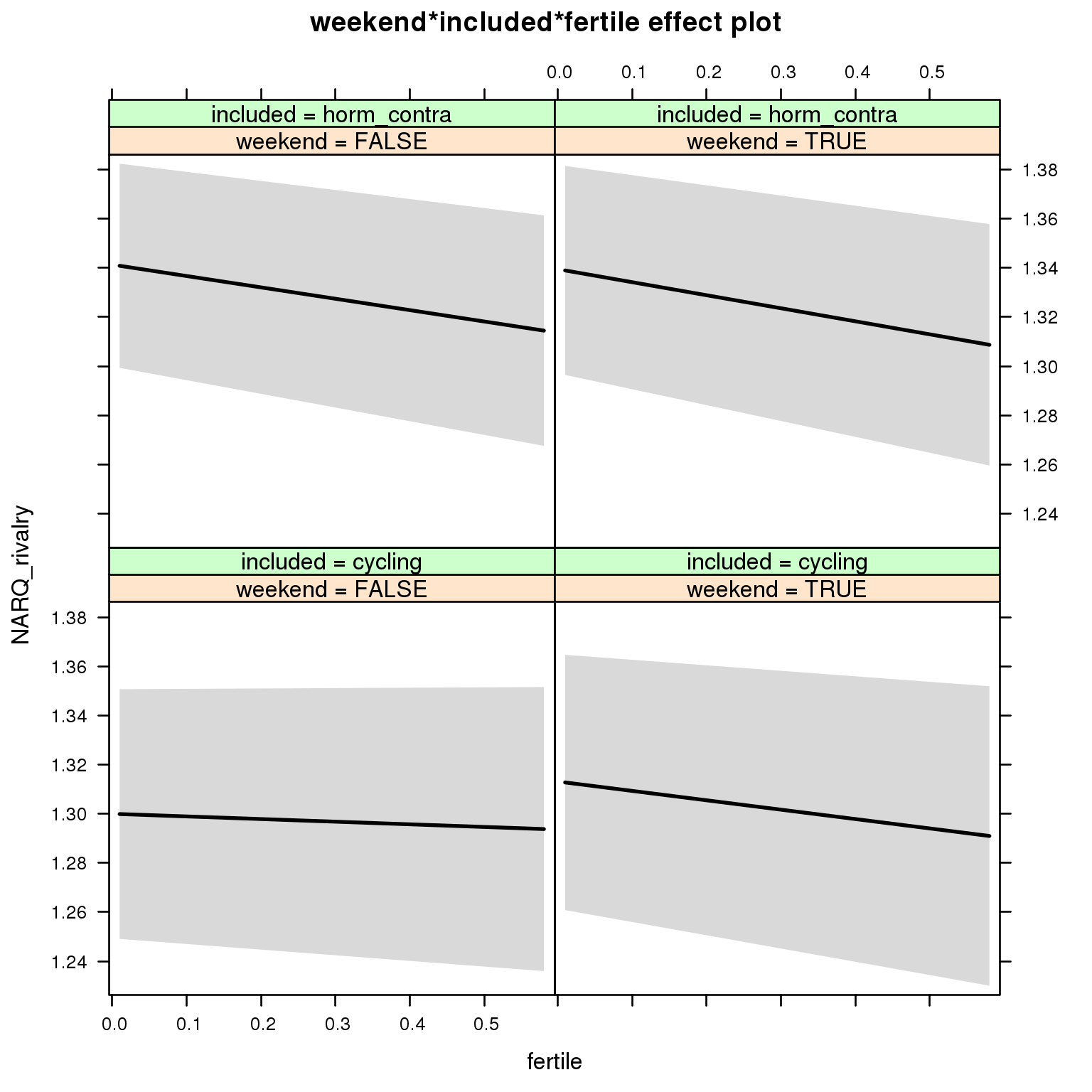
Linear mixed model fit by REML ['lmerMod']
Formula: NARQ_rivalry ~ menstruation + fertile_mean + (1 | person) + weekend +
included + fertile + menstruation:included + weekend:included +
weekend:fertile + included:fertile + weekend:included:fertile
Data: diary
REML criterion at convergence: 41889
Scaled residuals:
Min 1Q Median 3Q Max
-4.961 -0.327 -0.090 -0.011 9.682
Random effects:
Groups Name Variance Std.Dev.
person (Intercept) 0.240 0.490
Residual 0.249 0.499
Number of obs: 26681, groups: person, 1054
Fixed effects:
Estimate Std. Error t value
(Intercept) 1.288146 0.041640 30.94
menstruationpre -0.017910 0.015263 -1.17
menstruationyes 0.004019 0.014390 0.28
fertile_mean 0.082595 0.188209 0.44
weekendTRUE 0.013130 0.013294 0.99
includedhorm_contra 0.044653 0.034602 1.29
fertile -0.010713 0.037461 -0.29
menstruationpre:includedhorm_contra 0.000363 0.019595 0.02
menstruationyes:includedhorm_contra -0.019676 0.018862 -1.04
weekendTRUE:includedhorm_contra -0.014957 0.017111 -0.87
weekendTRUE:fertile -0.027490 0.051559 -0.53
includedhorm_contra:fertile -0.035562 0.047611 -0.75
weekendTRUE:includedhorm_contra:fertile 0.020692 0.065574 0.32
M_m4: Moderation by weekday
model %>%
test_moderator("weekday", diary, xlevels = 7)refitting model(s) with ML (instead of REML)
| Df | AIC | BIC | logLik | deviance | Chisq | Chi Df | Pr(>Chisq) | |
|---|---|---|---|---|---|---|---|---|
| with_main | 23 | 41843 | 42032 | -20899 | 41797 | NA | NA | NA |
| with_mod | 35 | 41857 | 42144 | -20893 | 41787 | 10.38 | 12 | 0.5828 |
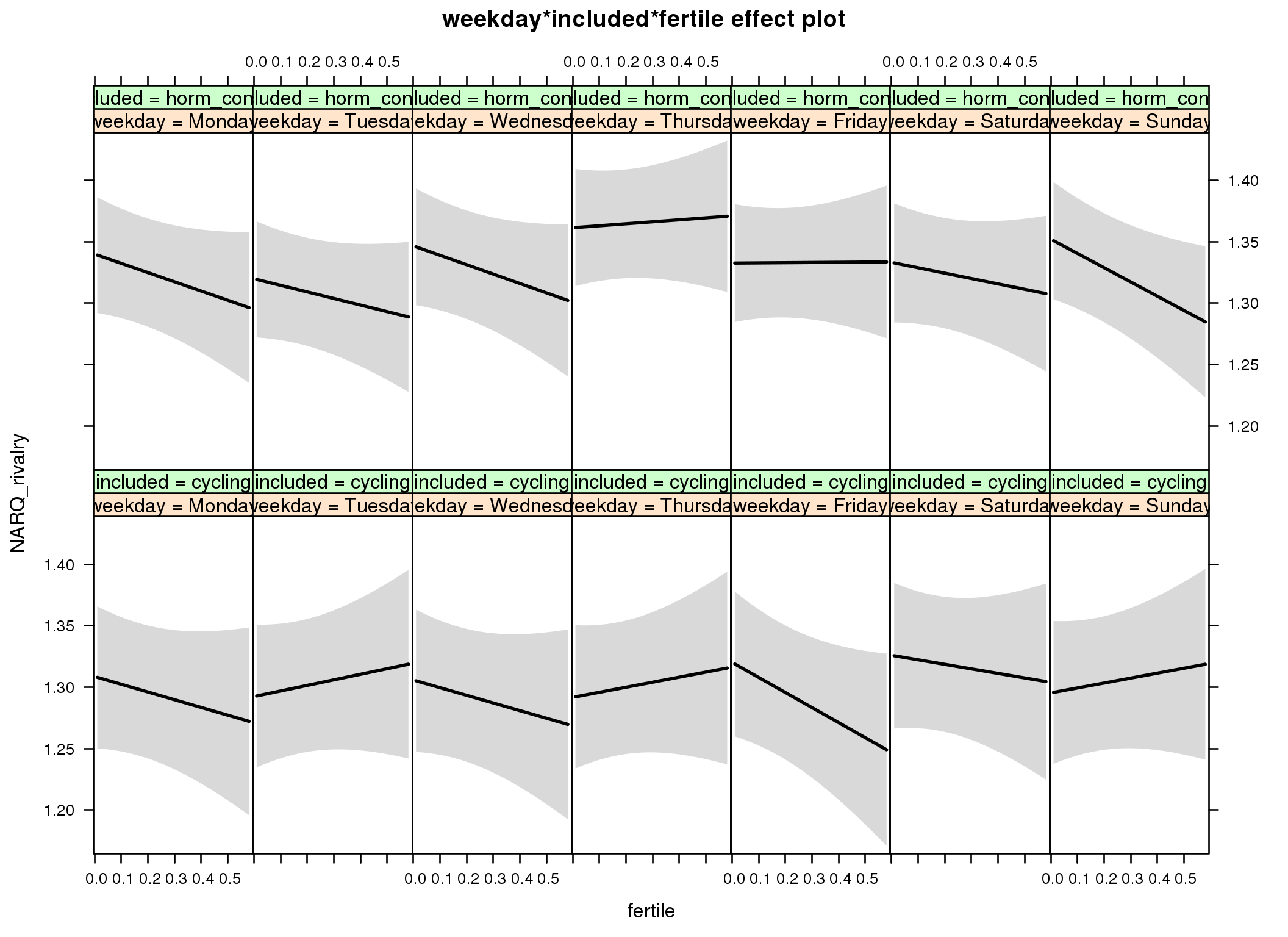
Linear mixed model fit by REML ['lmerMod']
Formula: NARQ_rivalry ~ menstruation + fertile_mean + (1 | person) + weekday +
included + fertile + menstruation:included + weekday:included +
weekday:fertile + included:fertile + weekday:included:fertile
Data: diary
REML criterion at convergence: 41961
Scaled residuals:
Min 1Q Median 3Q Max
-5.002 -0.327 -0.096 0.000 9.692
Random effects:
Groups Name Variance Std.Dev.
person (Intercept) 0.240 0.490
Residual 0.249 0.499
Number of obs: 26681, groups: person, 1054
Fixed effects:
Estimate Std. Error t value
(Intercept) 1.2965264 0.0440958 29.40
menstruationpre -0.0180061 0.0152640 -1.18
menstruationyes 0.0040177 0.0143896 0.28
fertile_mean 0.0842344 0.1882063 0.45
weekdayTuesday -0.0162531 0.0237818 -0.68
weekdayWednesday -0.0028287 0.0237432 -0.12
weekdayThursday -0.0169188 0.0240135 -0.70
weekdayFriday 0.0114869 0.0244195 0.47
weekdaySaturday 0.0173214 0.0246741 0.70
weekdaySunday -0.0132745 0.0238332 -0.56
includedhorm_contra 0.0346904 0.0392554 0.88
fertile -0.0628561 0.0669917 -0.94
menstruationpre:includedhorm_contra 0.0000536 0.0195958 0.00
menstruationyes:includedhorm_contra -0.0201228 0.0188625 -1.07
weekdayTuesday:includedhorm_contra -0.0038011 0.0305520 -0.12
weekdayWednesday:includedhorm_contra 0.0095375 0.0306524 0.31
weekdayThursday:includedhorm_contra 0.0384147 0.0309450 1.24
weekdayFriday:includedhorm_contra -0.0187864 0.0313711 -0.60
weekdaySaturday:includedhorm_contra -0.0240286 0.0317428 -0.76
weekdaySunday:includedhorm_contra 0.0254212 0.0307622 0.83
weekdayTuesday:fertile 0.1082040 0.0922183 1.17
weekdayWednesday:fertile 0.0006004 0.0926438 0.01
weekdayThursday:fertile 0.1039889 0.0939725 1.11
weekdayFriday:fertile -0.0596343 0.0941275 -0.63
weekdaySaturday:fertile 0.0260036 0.0953931 0.27
weekdaySunday:fertile 0.1029867 0.0926970 1.11
includedhorm_contra:fertile -0.0122118 0.0856991 -0.14
weekdayTuesday:includedhorm_contra:fertile -0.0866164 0.1176962 -0.74
weekdayWednesday:includedhorm_contra:fertile -0.0020464 0.1186211 -0.02
weekdayThursday:includedhorm_contra:fertile -0.0127724 0.1195750 -0.11
weekdayFriday:includedhorm_contra:fertile 0.1363753 0.1199441 1.14
weekdaySaturday:includedhorm_contra:fertile 0.0052706 0.1216820 0.04
weekdaySunday:includedhorm_contra:fertile -0.1439171 0.1184018 -1.22
M_m5: Moderation by exclusion threshold
model %>%
test_moderator("included_levels", diary, xlevels = 4)refitting model(s) with ML (instead of REML)
| Df | AIC | BIC | logLik | deviance | Chisq | Chi Df | Pr(>Chisq) | |
|---|---|---|---|---|---|---|---|---|
| with_main | 17 | 41847 | 41986 | -20906 | 41813 | NA | NA | NA |
| with_mod | 23 | 41847 | 42035 | -20900 | 41801 | 12.29 | 6 | 0.05587 |
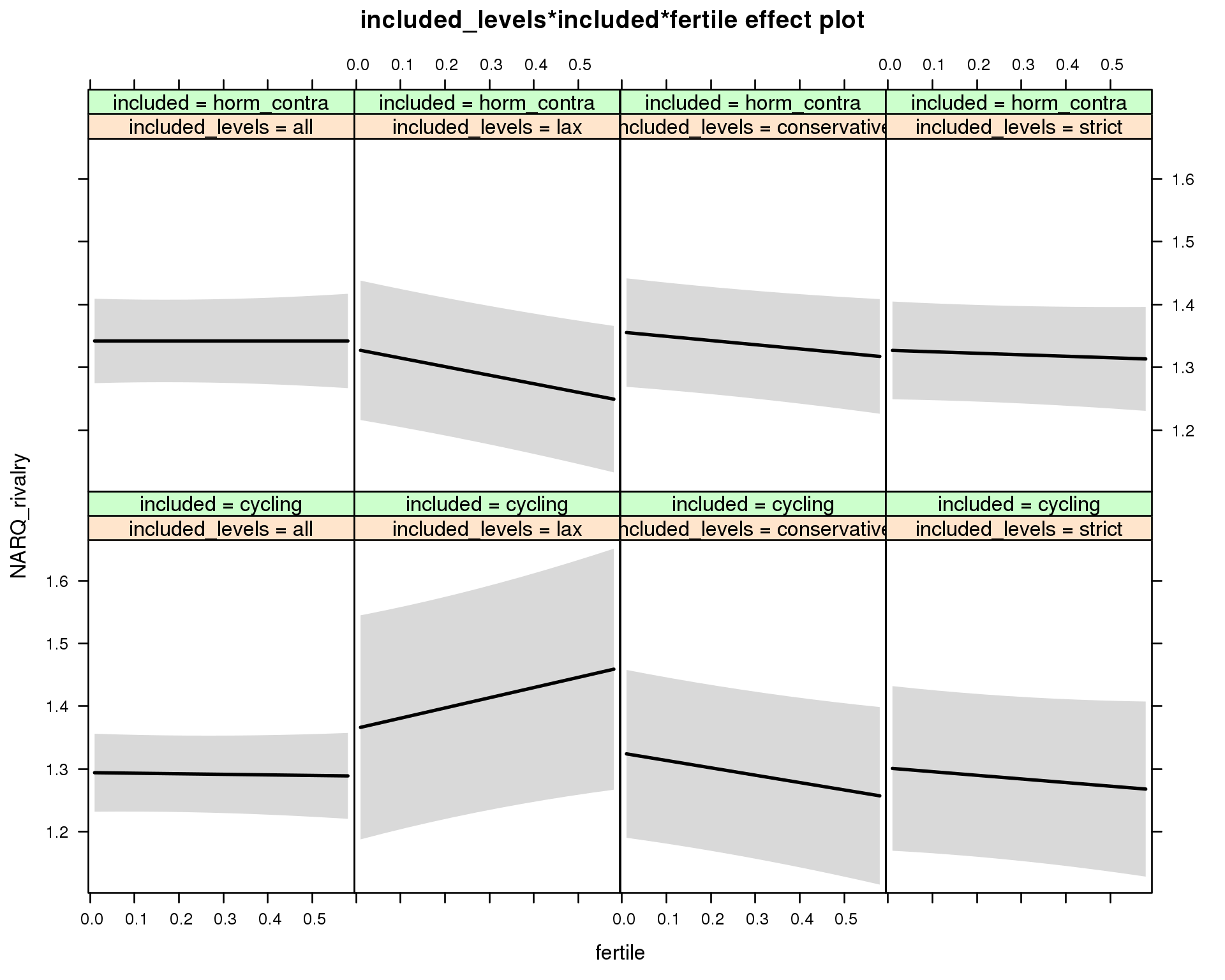
Linear mixed model fit by REML ['lmerMod']
Formula: NARQ_rivalry ~ menstruation + fertile_mean + (1 | person) + included_levels +
included + fertile + menstruation:included + included_levels:included +
included_levels:fertile + included:fertile + included_levels:included:fertile
Data: diary
REML criterion at convergence: 41896
Scaled residuals:
Min 1Q Median 3Q Max
-4.970 -0.328 -0.092 -0.009 9.660
Random effects:
Groups Name Variance Std.Dev.
person (Intercept) 0.242 0.491
Residual 0.249 0.499
Number of obs: 26681, groups: person, 1054
Fixed effects:
Estimate Std. Error t value
(Intercept) 1.284835 0.045943 27.97
menstruationpre -0.018531 0.015275 -1.21
menstruationyes 0.003119 0.014394 0.22
fertile_mean 0.069886 0.189989 0.37
included_levelslax 0.070523 0.096432 0.73
included_levelsconservative 0.031085 0.075195 0.41
included_levelsstrict 0.007298 0.074016 0.10
includedhorm_contra 0.051034 0.047454 1.08
fertile -0.008917 0.038946 -0.23
menstruationpre:includedhorm_contra 0.000584 0.019615 0.03
menstruationyes:includedhorm_contra -0.019551 0.018883 -1.04
included_levelslax:includedhorm_contra -0.084132 0.117185 -0.72
included_levelsconservative:includedhorm_contra -0.017097 0.093729 -0.18
included_levelsstrict:includedhorm_contra -0.022125 0.090761 -0.24
included_levelslax:fertile 0.171363 0.095042 1.80
included_levelsconservative:fertile -0.108314 0.070989 -1.53
included_levelsstrict:fertile -0.048736 0.071034 -0.69
includedhorm_contra:fertile 0.008849 0.059580 0.15
included_levelslax:includedhorm_contra:fertile -0.307670 0.116010 -2.65
included_levelsconservative:includedhorm_contra:fertile 0.041771 0.092363 0.45
included_levelsstrict:includedhorm_contra:fertile 0.025006 0.090939 0.27
M_m6: Moderation by cycle length
model %>%
test_moderator("cycle_length_groups", diary, xlevels = 4)refitting model(s) with ML (instead of REML)
| Df | AIC | BIC | logLik | deviance | Chisq | Chi Df | Pr(>Chisq) | |
|---|---|---|---|---|---|---|---|---|
| with_main | 17 | 41836 | 41975 | -20901 | 41802 | NA | NA | NA |
| with_mod | 23 | 41845 | 42033 | -20899 | 41799 | 3.471 | 6 | 0.7478 |
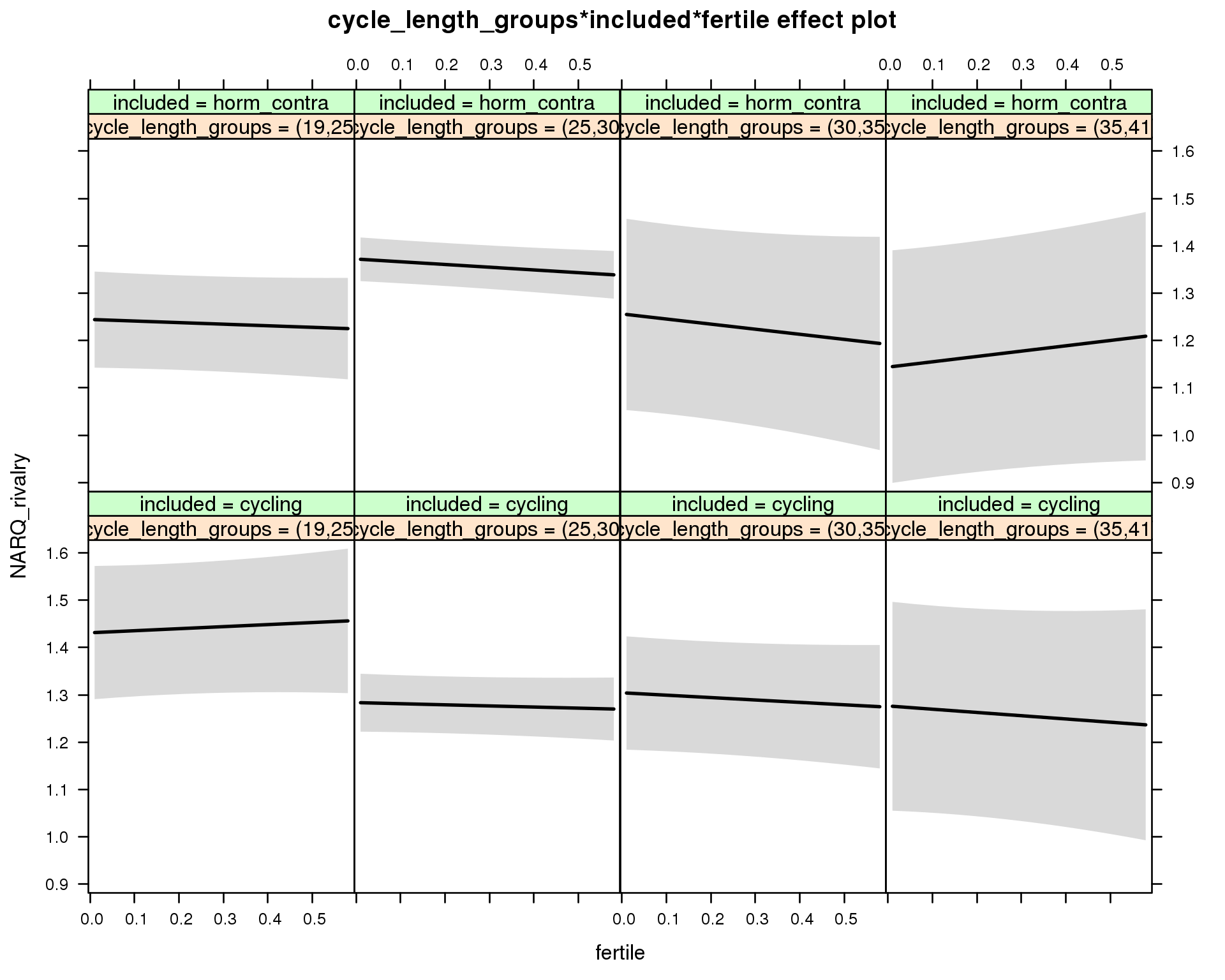
Linear mixed model fit by REML ['lmerMod']
Formula: NARQ_rivalry ~ menstruation + fertile_mean + (1 | person) + cycle_length_groups +
included + fertile + menstruation:included + cycle_length_groups:included +
cycle_length_groups:fertile + included:fertile + cycle_length_groups:included:fertile
Data: diary
REML criterion at convergence: 41886
Scaled residuals:
Min 1Q Median 3Q Max
-4.965 -0.329 -0.091 -0.010 9.693
Random effects:
Groups Name Variance Std.Dev.
person (Intercept) 0.239 0.489
Residual 0.249 0.499
Number of obs: 26681, groups: person, 1054
Fixed effects:
Estimate Std. Error t value
(Intercept) 1.421635 0.079537 17.87
menstruationpre -0.018324 0.015285 -1.20
menstruationyes 0.002494 0.014497 0.17
fertile_mean 0.071479 0.190151 0.38
cycle_length_groups(25,30] -0.147488 0.078345 -1.88
cycle_length_groups(30,35] -0.126745 0.094387 -1.34
cycle_length_groups(35,41] -0.154579 0.133679 -1.16
includedhorm_contra -0.183585 0.089002 -2.06
fertile 0.043191 0.081333 0.53
menstruationpre:includedhorm_contra 0.000592 0.019615 0.03
menstruationyes:includedhorm_contra -0.018715 0.018975 -0.99
cycle_length_groups(25,30]:includedhorm_contra 0.275120 0.096841 2.84
cycle_length_groups(30,35]:includedhorm_contra 0.138355 0.148961 0.93
cycle_length_groups(35,41]:includedhorm_contra 0.053900 0.190204 0.28
cycle_length_groups(25,30]:fertile -0.066611 0.087265 -0.76
cycle_length_groups(30,35]:fertile -0.093908 0.103307 -0.91
cycle_length_groups(35,41]:fertile -0.111873 0.145909 -0.77
includedhorm_contra:fertile -0.076485 0.096006 -0.80
cycle_length_groups(25,30]:includedhorm_contra:fertile 0.042351 0.103369 0.41
cycle_length_groups(30,35]:includedhorm_contra:fertile 0.019781 0.162618 0.12
cycle_length_groups(35,41]:includedhorm_contra:fertile 0.257706 0.192108 1.34
M_m7: Moderation by certainty about menstruation parameters
model %>%
test_moderator("certainty_menstruation", diary)refitting model(s) with ML (instead of REML)
| Df | AIC | BIC | logLik | deviance | Chisq | Chi Df | Pr(>Chisq) | |
|---|---|---|---|---|---|---|---|---|
| with_main | 13 | 41833 | 41939 | -20903 | 41807 | NA | NA | NA |
| with_mod | 15 | 41832 | 41955 | -20901 | 41802 | 4.925 | 2 | 0.08524 |
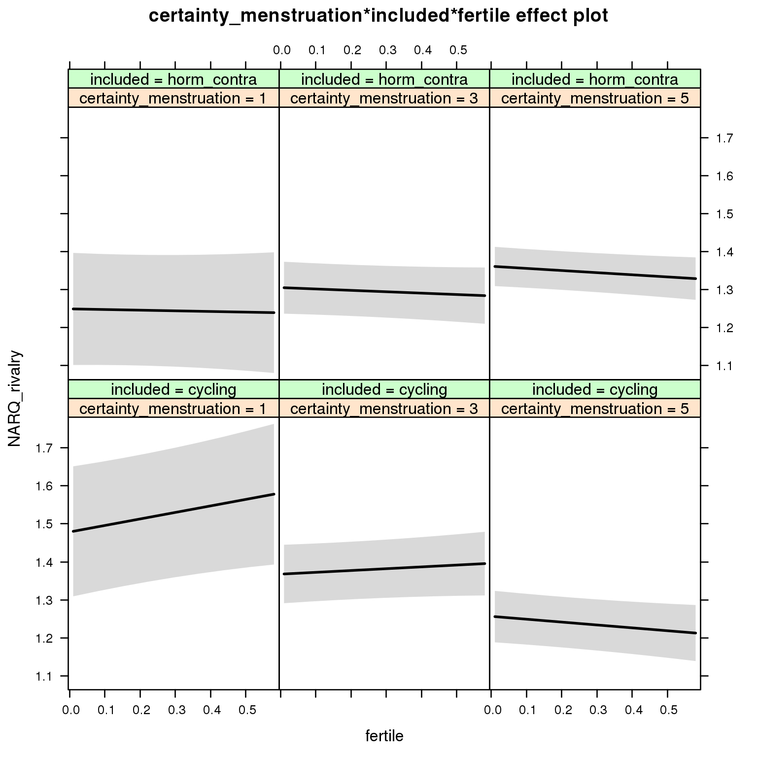
Linear mixed model fit by REML ['lmerMod']
Formula: NARQ_rivalry ~ menstruation + fertile_mean + (1 | person) + certainty_menstruation +
included + fertile + menstruation:included + certainty_menstruation:included +
certainty_menstruation:fertile + included:fertile + certainty_menstruation:included:fertile
Data: diary
REML criterion at convergence: 41876
Scaled residuals:
Min 1Q Median 3Q Max
-4.965 -0.328 -0.091 -0.009 9.686
Random effects:
Groups Name Variance Std.Dev.
person (Intercept) 0.239 0.489
Residual 0.249 0.499
Number of obs: 26681, groups: person, 1054
Fixed effects:
Estimate Std. Error t value
(Intercept) 1.52478 0.11760 12.97
menstruationpre -0.01908 0.01527 -1.25
menstruationyes 0.00237 0.01441 0.16
fertile_mean 0.07147 0.18815 0.38
certainty_menstruation -0.05553 0.02682 -2.07
includedhorm_contra -0.31035 0.14935 -2.08
fertile 0.23349 0.12125 1.93
menstruationpre:includedhorm_contra 0.00155 0.01960 0.08
menstruationyes:includedhorm_contra -0.01814 0.01888 -0.96
certainty_menstruation:includedhorm_contra 0.08358 0.03481 2.40
certainty_menstruation:fertile -0.06187 0.02841 -2.18
includedhorm_contra:fertile -0.24084 0.15761 -1.53
certainty_menstruation:includedhorm_contra:fertile 0.05212 0.03643 1.43
M_m8: Moderation by cycle regularity
model %>%
test_moderator("cycle_regularity", diary)refitting model(s) with ML (instead of REML)
| Df | AIC | BIC | logLik | deviance | Chisq | Chi Df | Pr(>Chisq) | |
|---|---|---|---|---|---|---|---|---|
| with_main | 15 | 41840 | 41963 | -20905 | 41810 | NA | NA | NA |
| with_mod | 19 | 41848 | 42003 | -20905 | 41810 | 0.668 | 4 | 0.9552 |
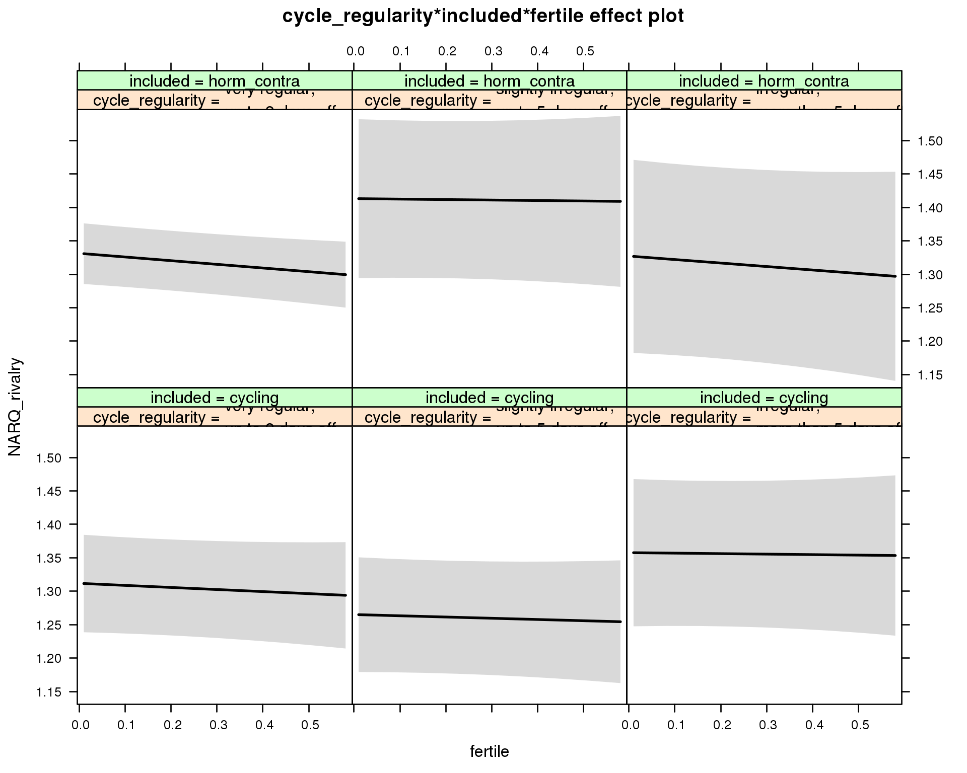
Linear mixed model fit by REML ['lmerMod']
Formula: NARQ_rivalry ~ menstruation + fertile_mean + (1 | person) + cycle_regularity +
included + fertile + menstruation:included + cycle_regularity:included +
cycle_regularity:fertile + included:fertile + cycle_regularity:included:fertile
Data: diary
REML criterion at convergence: 41890
Scaled residuals:
Min 1Q Median 3Q Max
-4.964 -0.327 -0.090 -0.011 9.683
Random effects:
Groups Name Variance Std.Dev.
person (Intercept) 0.24 0.49
Residual 0.25 0.50
Number of obs: 26681, groups: person, 1054
Fixed effects:
Estimate Std. Error
(Intercept) 1.295018 0.048865
menstruationpre -0.018019 0.015275
menstruationyes 0.003995 0.014397
fertile_mean 0.111200 0.189183
cycle_regularityslightly irregular,\nup to 5 days off -0.046703 0.057450
cycle_regularityirregular,\nmore than 5 days off 0.045909 0.067341
includedhorm_contra 0.022991 0.044716
fertile -0.030923 0.042656
menstruationpre:includedhorm_contra 0.000466 0.019606
menstruationyes:includedhorm_contra -0.019686 0.018873
cycle_regularityslightly irregular,\nup to 5 days off:includedhorm_contra 0.128537 0.086868
cycle_regularityirregular,\nmore than 5 days off:includedhorm_contra -0.050023 0.102552
cycle_regularityslightly irregular,\nup to 5 days off:fertile 0.012425 0.058855
cycle_regularityirregular,\nmore than 5 days off:fertile 0.023551 0.072397
includedhorm_contra:fertile -0.024067 0.049986
cycle_regularityslightly irregular,\nup to 5 days off:includedhorm_contra:fertile 0.035485 0.087365
cycle_regularityirregular,\nmore than 5 days off:includedhorm_contra:fertile -0.020778 0.107967
t value
(Intercept) 26.50
menstruationpre -1.18
menstruationyes 0.28
fertile_mean 0.59
cycle_regularityslightly irregular,\nup to 5 days off -0.81
cycle_regularityirregular,\nmore than 5 days off 0.68
includedhorm_contra 0.51
fertile -0.72
menstruationpre:includedhorm_contra 0.02
menstruationyes:includedhorm_contra -1.04
cycle_regularityslightly irregular,\nup to 5 days off:includedhorm_contra 1.48
cycle_regularityirregular,\nmore than 5 days off:includedhorm_contra -0.49
cycle_regularityslightly irregular,\nup to 5 days off:fertile 0.21
cycle_regularityirregular,\nmore than 5 days off:fertile 0.33
includedhorm_contra:fertile -0.48
cycle_regularityslightly irregular,\nup to 5 days off:includedhorm_contra:fertile 0.41
cycle_regularityirregular,\nmore than 5 days off:includedhorm_contra:fertile -0.19
M_m9: Moderation by cohabitation status
model %>%
test_moderator("cohabitation", diary)refitting model(s) with ML (instead of REML)
| Df | AIC | BIC | logLik | deviance | Chisq | Chi Df | Pr(>Chisq) | |
|---|---|---|---|---|---|---|---|---|
| with_main | 15 | 41839 | 41962 | -20905 | 41809 | NA | NA | NA |
| with_mod | 19 | 41838 | 41994 | -20900 | 41800 | 9.086 | 4 | 0.05898 |
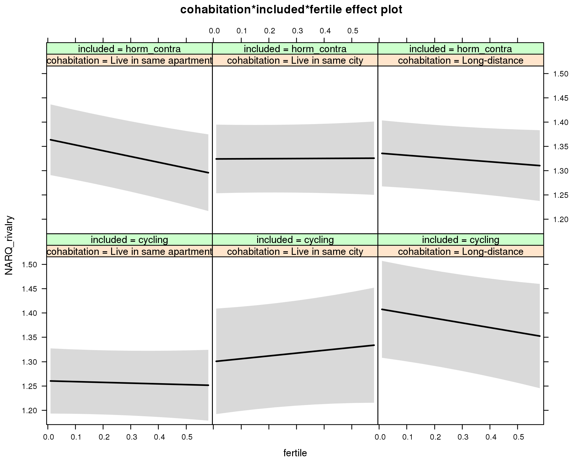
Linear mixed model fit by REML ['lmerMod']
Formula: NARQ_rivalry ~ menstruation + fertile_mean + (1 | person) + cohabitation +
included + fertile + menstruation:included + cohabitation:included +
cohabitation:fertile + included:fertile + cohabitation:included:fertile
Data: diary
REML criterion at convergence: 41884
Scaled residuals:
Min 1Q Median 3Q Max
-4.983 -0.326 -0.093 -0.010 9.687
Random effects:
Groups Name Variance Std.Dev.
person (Intercept) 0.240 0.490
Residual 0.249 0.499
Number of obs: 26681, groups: person, 1054
Fixed effects:
Estimate Std. Error t value
(Intercept) 1.248721 0.047339 26.38
menstruationpre -0.017865 0.015261 -1.17
menstruationyes 0.004497 0.014391 0.31
fertile_mean 0.081027 0.188493 0.43
cohabitationLive in same city 0.039715 0.065102 0.61
cohabitationLong-distance 0.148206 0.061303 2.42
includedhorm_contra 0.107664 0.051209 2.10
fertile -0.015390 0.038505 -0.40
menstruationpre:includedhorm_contra 0.000708 0.019594 0.04
menstruationyes:includedhorm_contra -0.020032 0.018861 -1.06
cohabitationLive in same city:includedhorm_contra -0.080388 0.083213 -0.97
cohabitationLong-distance:includedhorm_contra -0.176989 0.079622 -2.22
cohabitationLive in same city:fertile 0.073576 0.070399 1.05
cohabitationLong-distance:fertile -0.081066 0.063396 -1.28
includedhorm_contra:fertile -0.103547 0.056276 -1.84
cohabitationLive in same city:includedhorm_contra:fertile 0.048042 0.088008 0.55
cohabitationLong-distance:includedhorm_contra:fertile 0.155874 0.081644 1.91
M_m10: Moderation by relationship status
model %>%
test_moderator("relationship_status_clean", diary)refitting model(s) with ML (instead of REML)
| Df | AIC | BIC | logLik | deviance | Chisq | Chi Df | Pr(>Chisq) | |
|---|---|---|---|---|---|---|---|---|
| with_main | 15 | 41841 | 41964 | -20906 | 41811 | NA | NA | NA |
| with_mod | 19 | 41843 | 41998 | -20902 | 41805 | 6.936 | 4 | 0.1393 |
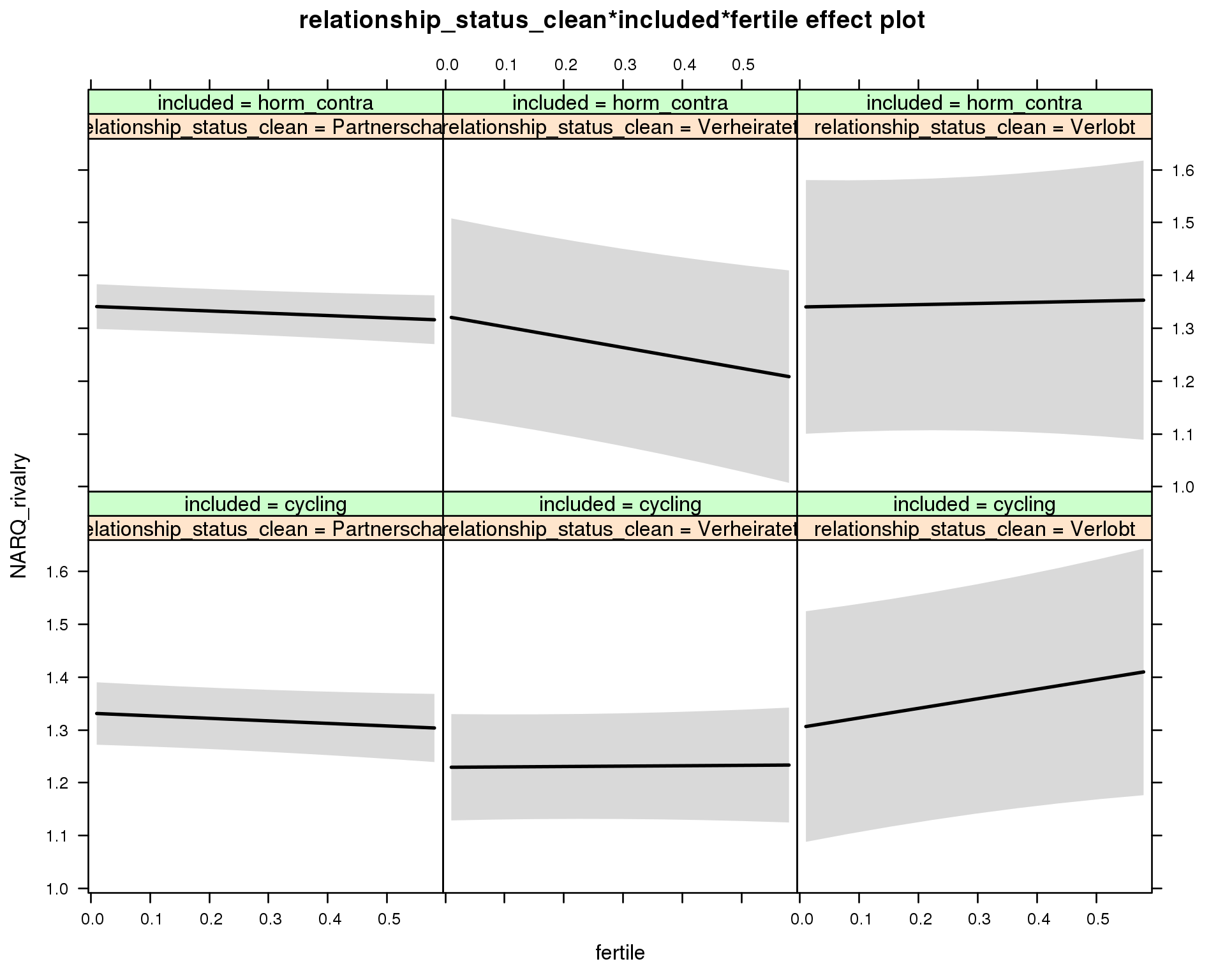
Linear mixed model fit by REML ['lmerMod']
Formula: NARQ_rivalry ~ menstruation + fertile_mean + (1 | person) + relationship_status_clean +
included + fertile + menstruation:included + relationship_status_clean:included +
relationship_status_clean:fertile + included:fertile + relationship_status_clean:included:fertile
Data: diary
REML criterion at convergence: 41879
Scaled residuals:
Min 1Q Median 3Q Max
-5.008 -0.328 -0.090 -0.009 9.686
Random effects:
Groups Name Variance Std.Dev.
person (Intercept) 0.241 0.491
Residual 0.249 0.499
Number of obs: 26681, groups: person, 1054
Fixed effects:
Estimate Std. Error t value
(Intercept) 1.319200 0.044360 29.74
menstruationpre -0.017834 0.015262 -1.17
menstruationyes 0.004018 0.014389 0.28
fertile_mean 0.086289 0.188566 0.46
relationship_status_cleanVerheiratet -0.102327 0.059533 -1.72
relationship_status_cleanVerlobt -0.026927 0.115531 -0.23
includedhorm_contra 0.013131 0.038113 0.34
fertile -0.048056 0.035272 -1.36
menstruationpre:includedhorm_contra 0.000371 0.019594 0.02
menstruationyes:includedhorm_contra -0.019565 0.018860 -1.04
relationship_status_cleanVerheiratet:includedhorm_contra 0.083295 0.114870 0.73
relationship_status_cleanVerlobt:includedhorm_contra 0.025694 0.169960 0.15
relationship_status_cleanVerheiratet:fertile 0.055386 0.062100 0.89
relationship_status_cleanVerlobt:fertile 0.229362 0.116480 1.97
includedhorm_contra:fertile 0.004417 0.043012 0.10
relationship_status_cleanVerheiratet:includedhorm_contra:fertile -0.208355 0.116937 -1.78
relationship_status_cleanVerlobt:includedhorm_contra:fertile -0.163386 0.180858 -0.90
Self esteem
model_summaries$self_esteem_1Model summary
Model summary
model %>%
print_summary()Linear mixed model fit by REML
t-tests use Satterthwaite approximations to degrees of freedom ['lmerMod']
Formula: self_esteem_1 ~ included * (menstruation + fertile) + fertile_mean + (1 | person)
Data: diary
REML criterion at convergence: 72472
Scaled residuals:
Min 1Q Median 3Q Max
-5.258 -0.497 0.093 0.632 4.414
Random effects:
Groups Name Variance Std.Dev.
person (Intercept) 0.583 0.764
Residual 0.793 0.891
Number of obs: 26685, groups: person, 1054
Fixed effects:
Estimate Std. Error df t value Pr(>|t|)
(Intercept) 4.3384 0.0660 1388.0000 65.71 < 2e-16 ***
includedhorm_contra -0.0603 0.0541 1343.0000 -1.11 0.26513
menstruationpre -0.0527 0.0272 25977.0000 -1.94 0.05253 .
menstruationyes -0.1201 0.0256 26080.0000 -4.69 0.0000028 ***
fertile -0.0779 0.0549 25964.0000 -1.42 0.15555
fertile_mean -0.2053 0.3023 1507.0000 -0.68 0.49715
includedhorm_contra:menstruationpre 0.0546 0.0349 25973.0000 1.57 0.11755
includedhorm_contra:menstruationyes 0.1219 0.0336 26059.0000 3.63 0.00029 ***
includedhorm_contra:fertile 0.1449 0.0695 26083.0000 2.08 0.03711 *
---
Signif. codes: 0 '***' 0.001 '**' 0.01 '*' 0.05 '.' 0.1 ' ' 1
Correlation of Fixed Effects:
(Intr) incld_ mnstrtnp mnstrtny fertil frtl_m inclddhrm_cntr:mnstrtnp
inclddhrm_c -0.473
menstrutnpr -0.158 0.201
menstrutnys -0.154 0.193 0.397
fertile -0.152 0.248 0.467 0.385
fertile_men -0.772 -0.025 -0.008 -0.005 -0.065
inclddhrm_cntr:mnstrtnp 0.131 -0.251 -0.779 -0.309 -0.363 -0.003
inclddhrm_cntr:mnstrtny 0.123 -0.238 -0.303 -0.763 -0.293 -0.003 0.383
inclddhrm_cntr:f 0.152 -0.314 -0.368 -0.303 -0.787 0.010 0.466
inclddhrm_cntr:mnstrtny
inclddhrm_c
menstrutnpr
menstrutnys
fertile
fertile_men
inclddhrm_cntr:mnstrtnp
inclddhrm_cntr:mnstrtny
inclddhrm_cntr:f 0.381
Effect size standardised by residual variance (\(\frac{b}{ SD_{residual} }\)): -0.09 [-0.21;0.03].
Marginal effect plots
model %>%
plot_all_effects()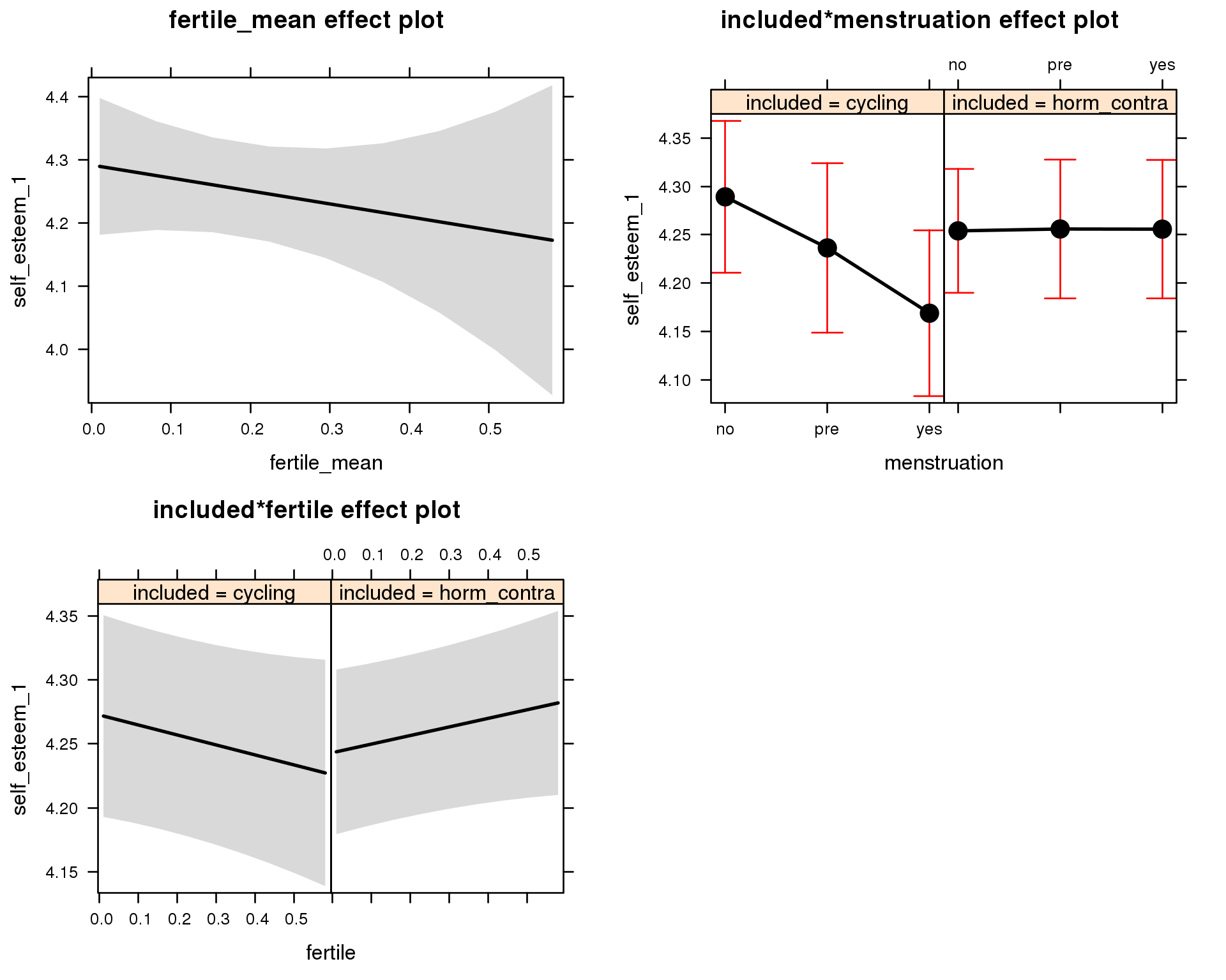
Outcome distribution
model %>%
plot_outcome(diary) + xlab(outcome_label)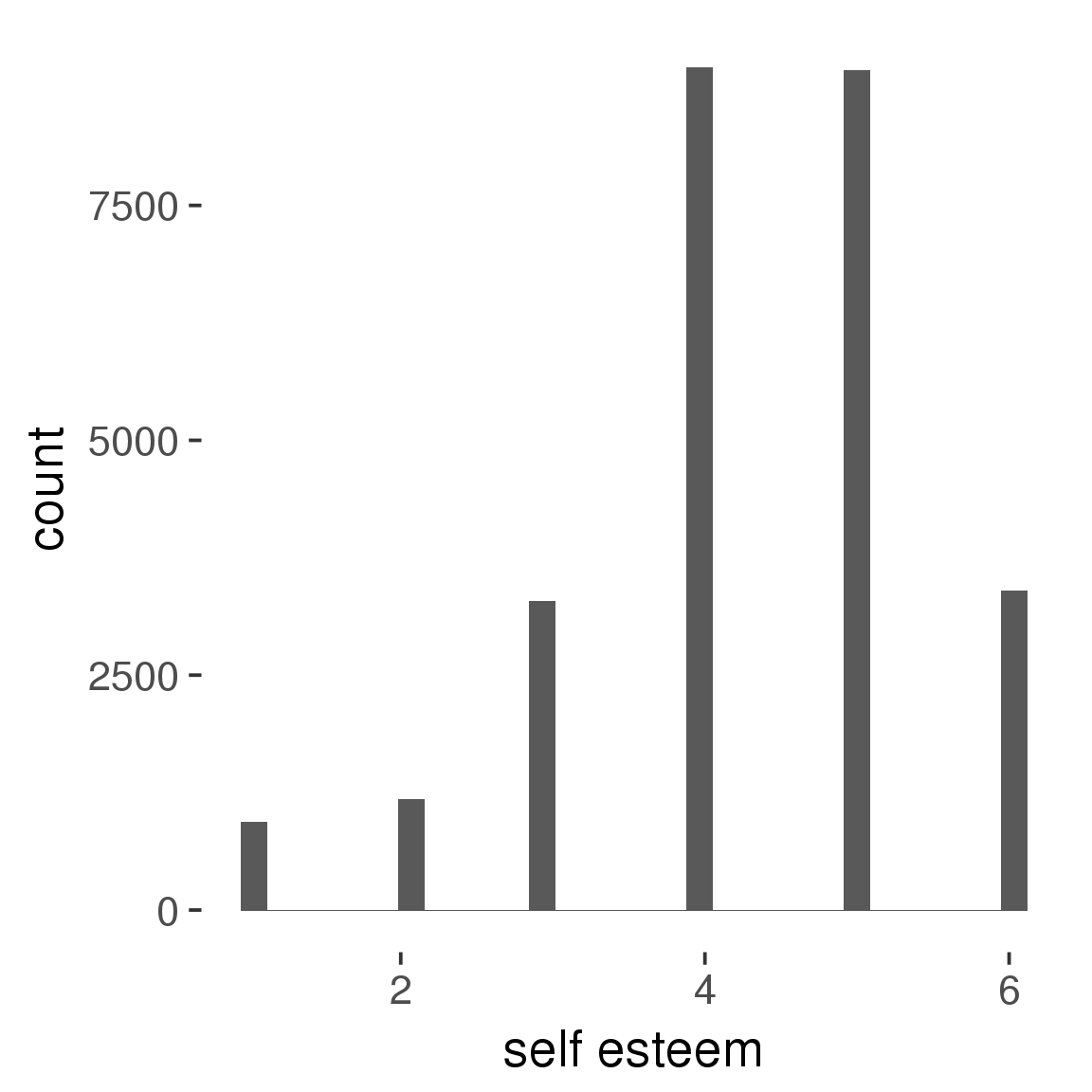
Diagnostics
model %>%
print_diagnostics()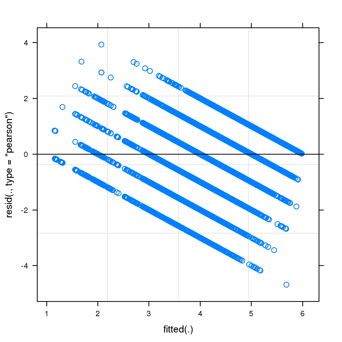
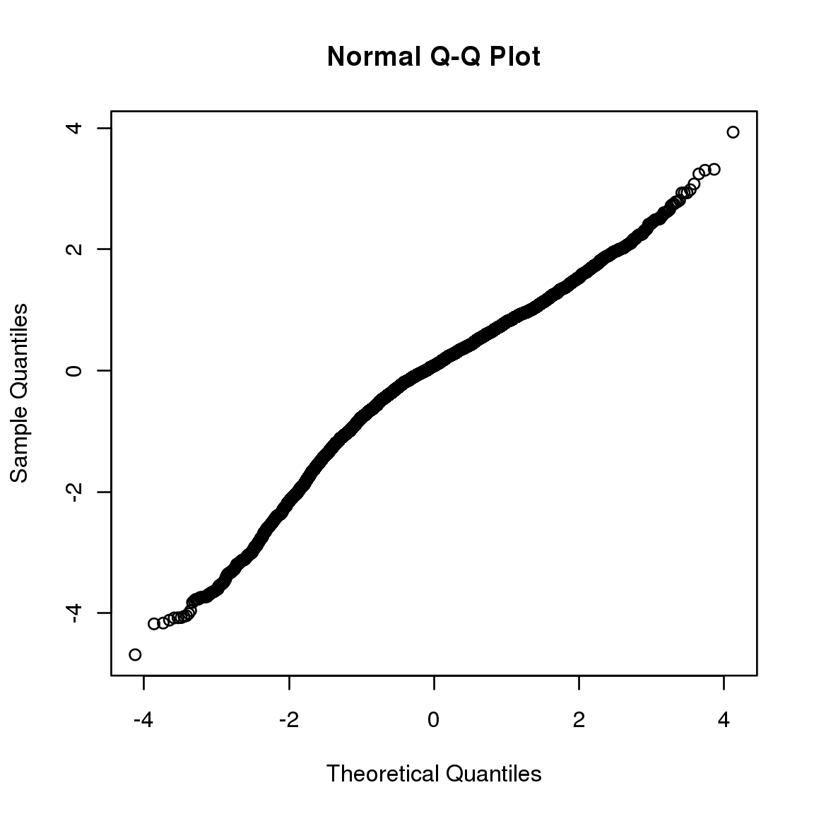

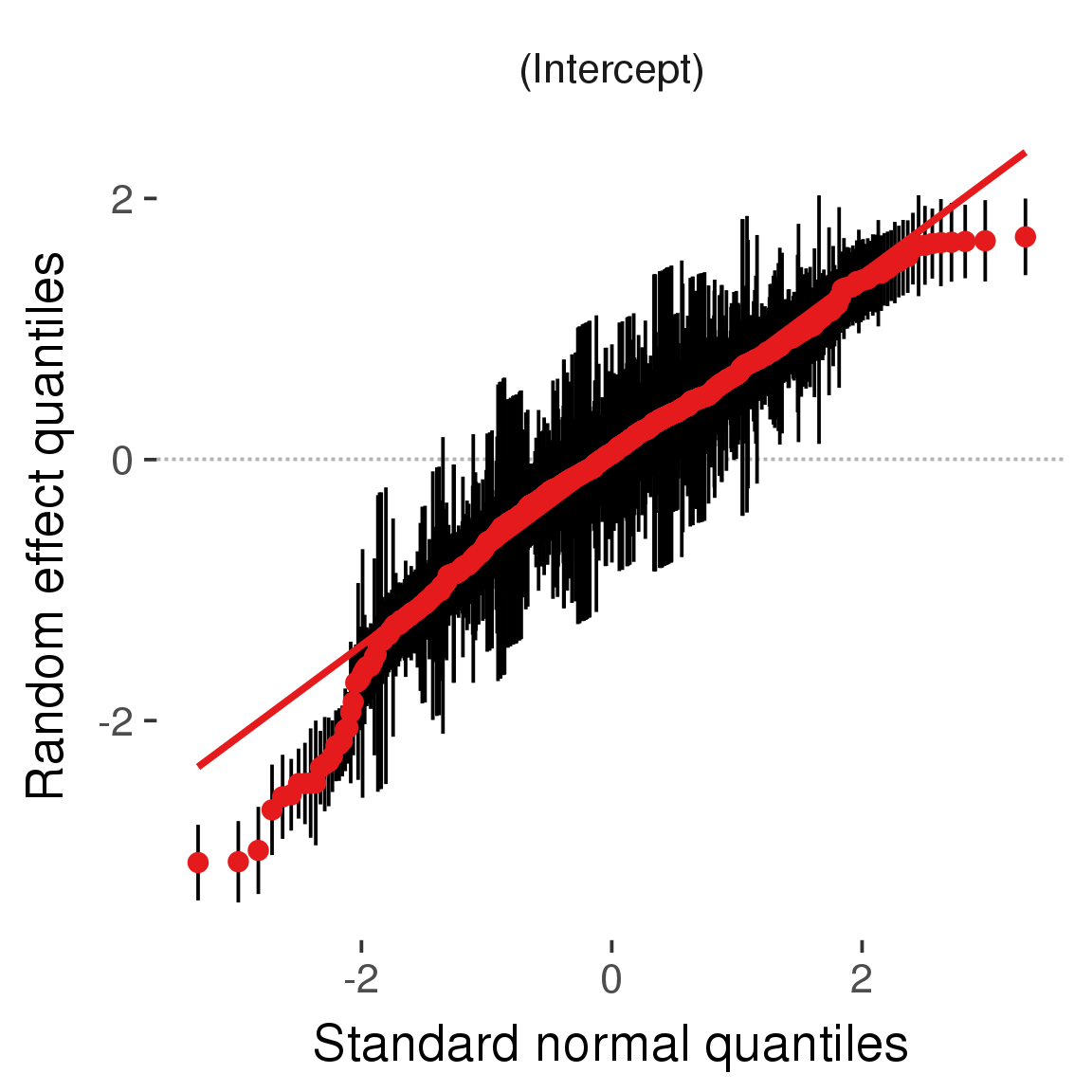
Curves
Here, we continuously plot the outcome over the course of the cycle. Because cycle lengths vary, we subset the data to cycles in a certain range. If the red curve traces the pink curve, our predictor accurately maps the relationship between fertile window probability and the outcome.
Cycle lengths from 21 to 36
Backward-counted
model %>%
plot_curve(diary %>% filter(minimum_cycle_length_diary <= 36, minimum_cycle_length_diary > 20) %>% mutate(fertile=prc_stirn_b))outcome = names(model@frame)[1]
outcome_label = recode(str_replace_all(str_replace_all(str_replace_all(outcome, "_", " "), " pair", "-pair"), " 1", ""),
"desirability 1" = "self-perceived desirability",
"NARQ admiration" = "narcissistic admiration",
"NARQ rivalry" = "narcissistic rivalry",
"extra-pair" = "extra-pair desire & behaviour",
"had sexual intercourse" = "sexual intercourse")
library(ggplot2)
# form a subset and run the model without the hormonal contraception and the fertility predictors
tmp = diary %>%
filter(!is.na(fertile), !is.na(included),
RCD > -1 * minimum_cycle_length_diary, RCD > -40)
new_form = update.formula(formula(model), new = . ~ . - fertile * included)
tmp$residuals = residuals(update(model, new_form, data = tmp , na.action = na.exclude))
tmp = tmp %>%
filter(!is.na(RCD), !is.na(residuals))
rcd_min = min(tmp$RCD)
tmp$real = FALSE
tmp_before = tmp
tmp_before$RCD = tmp_before$RCD + min(tmp$RCD) - 1
tmp_after = tmp
tmp_after$RCD = tmp_after$RCD - min(tmp$RCD) + 1
tmp$real = TRUE
tmp = bind_rows(tmp_before %>% filter(RCD > rcd_min - 11), tmp, tmp_after %>% filter(RCD < 11))GAM smooth on residuals
Here, we partialled out menstruation and individual random effects, then superimposed estimated probability of being in the fertile window scaled to the range of the estimated means. To address the periodicity of the cycle, we prepended and appended ten days of the timeseries to the end and the beginning of the timeseries. We then estimated the GAM and cut off the appended subsets before plotting.
tryCatch({
trend_plot = ggplot(tmp,aes(x = RCD, y = residuals, colour = included)) +
stat_smooth(geom = 'smooth',size = 0.8, fill = "#9ECAE1", method = 'gam', formula = y ~ s(x))
}, error = function(e){cat_message(e, "danger")})
tryCatch({
trend_data = ggplot_build(trend_plot)$data[[1]]
}, error = function(e){cat_message(e, "danger")})
trend_data$RCD = round(trend_data$x)
trend_data = left_join(trend_data, tmp %>% select(real, RCD,fertile) %>% unique(), by = "RCD")
trend_data %>%
filter(real == TRUE) %>%
mutate(superimposed = ( ( (fertile - 0.01)/0.58) * (max(y)-min(y) ) ) + min(y) ) ->
trend_data
ggplot(trend_data) +
geom_ribbon(aes(x = x, ymin = ymin, ymax = ymax, fill = factor(group)), alpha = 0.2) +
geom_line(aes(x = x, y = y, colour = factor(group)), size = 0.8, stat = "identity") +
scale_x_continuous(caption_x) +
geom_line(aes(x = x, y = superimposed), color = "#a83fbf", size = 1, linetype = 'dashed') +
annotate("text",x = mean(trend_data$x), y = max(trend_data$superimposed,na.rm=T) + 0.1, label = 'superimposed fertility peak', color = "#a83fbf") +
scale_y_continuous(outcome_label) +
ggtitle("GAM smooth, residuals") +
scale_color_manual("Contraception status",values = c("2"="black","1"= "red"), labels = c("2"="hormonally\ncontracepting","1"="cycling"), guide = F) +
scale_fill_manual("Contraception status",values = c("2"="black","1"= "red"), labels = c("2"="hormonally\ncontracepting","1"="cycling"), guide = F)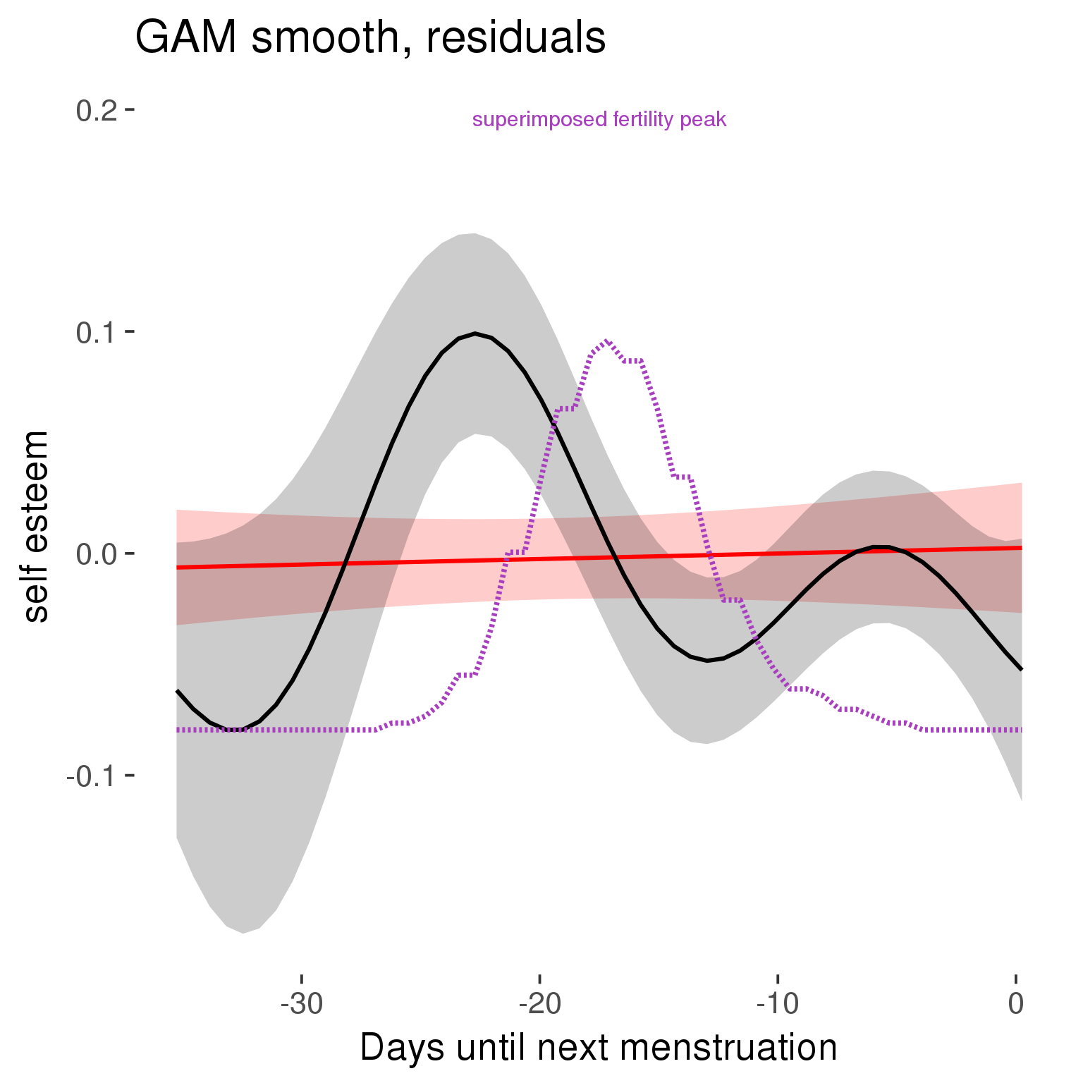
GAM smooth on raw data
As before, but without partialling anything out.
tryCatch({
trend_plot = ggplot(tmp,aes_string(x = "RCD", y = outcome, colour = "included")) +
stat_smooth(geom = 'smooth',size = 0.8, fill = "#9ECAE1", method = 'gam', formula = y ~ s(x))
}, error = function(e){cat_message(e, "danger")})
tryCatch({
trend_data = ggplot_build(trend_plot)$data[[1]]
}, error = function(e){cat_message(e, "danger")})
trend_data$RCD = round(trend_data$x)
trend_data = left_join(trend_data, tmp %>% select(real, RCD,fertile) %>% unique(), by = "RCD")
trend_data %>%
filter(real == TRUE) %>%
mutate(superimposed = ( ( (fertile - 0.01)/0.58) * (max(y)-min(y) ) ) + min(y) ) ->
trend_data
plot1b = ggplot(trend_data) +
geom_ribbon(aes(x = x, ymin = ymin, ymax = ymax, fill = factor(group)), alpha = 0.2) +
geom_line(aes(x = x, y = y, colour = factor(group)), size = 0.8, stat = "identity") +
scale_x_continuous(caption_x) +
geom_line(aes(x = x, y = superimposed), color = "#a83fbf", size = 1, linetype = 'dashed') +
annotate("text",x = mean(trend_data$x), y = max(trend_data$superimposed,na.rm=T) + 0.1, label = 'superimposed fertility peak', color = "#a83fbf") +
scale_y_continuous(outcome_label) +
ggtitle("GAM smooth, raw data") +
scale_color_manual("Contraception status",values = c("2"="black","1"= "red"), labels = c("2"="hormonally\ncontracepting","1"="cycling"), guide = F) +
scale_fill_manual("Contraception status",values = c("2"="black","1"= "red"), labels = c("2"="hormonally\ncontracepting","1"="cycling"), guide = F)
suppressWarnings(print(plot1b))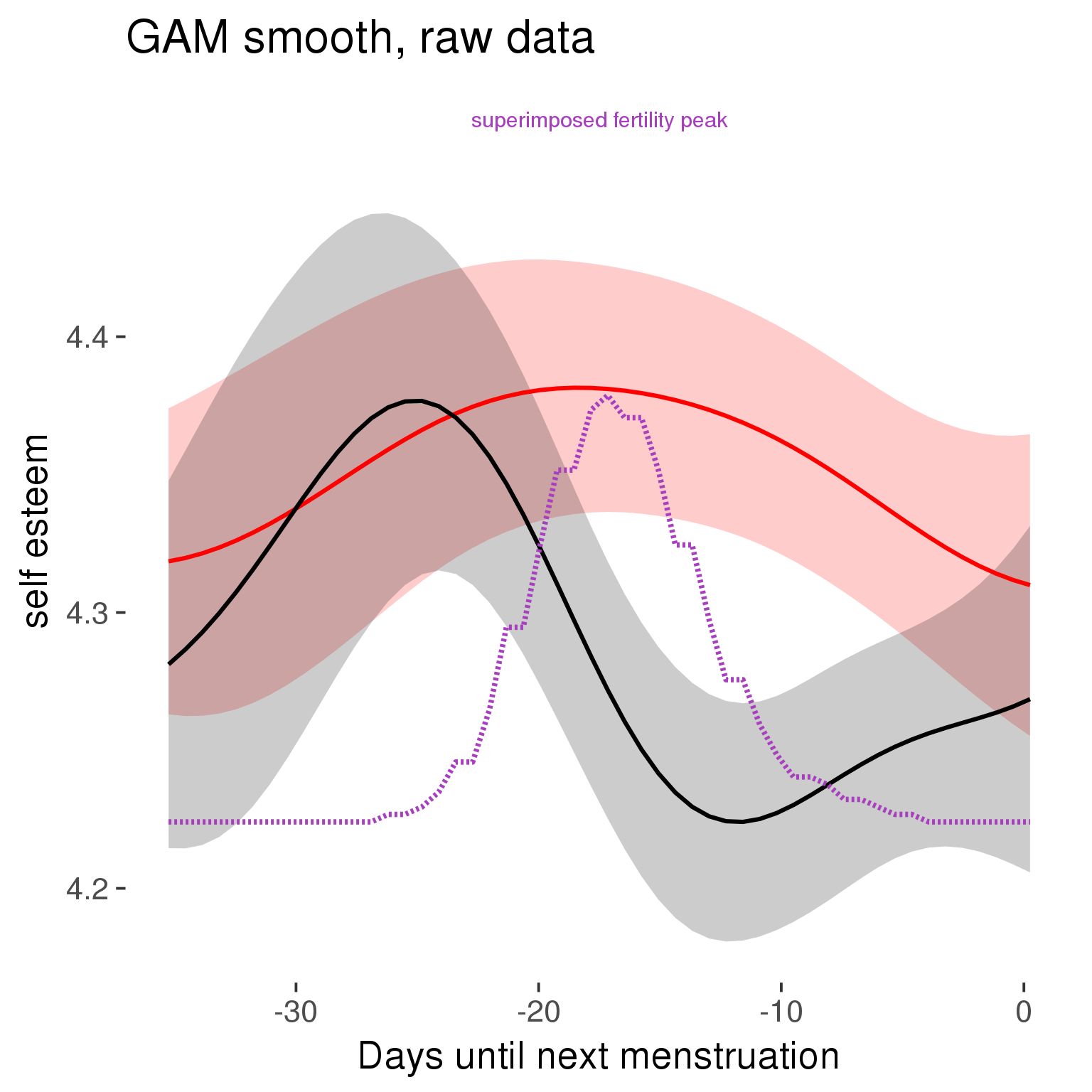
Means and standard errors over raw data
Nothing partialled out, just straight means with bootstrapped confidence intervals.
tryCatch({
trend_plot = ggplot(tmp,aes_string(x = "RCD", y = outcome, colour = "included")) +
geom_pointrange(size = 0.8, stat = 'summary', fun.data = "mean_cl_boot")
}, error = function(e){cat_message(e, "danger")})
tryCatch({
trend_data = ggplot_build(trend_plot)$data[[1]]
}, error = function(e){cat_message(e, "danger")})
trend_data$RCD = round(trend_data$x)
trend_data = left_join(trend_data, tmp %>% select(real, RCD,fertile) %>% unique(), by = "RCD")
trend_data %>%
filter(real == TRUE) %>%
mutate(superimposed = ( ( (fertile - 0.01)/0.58) * (max(y)-min(y) ) ) + min(y) ) ->
trend_data
plot3 = ggplot(trend_data) +
geom_pointrange(aes(x = x, y = y, ymin = ymin,ymax = ymax, colour = factor(group)), size = 0.8, stat = "identity", alpha = 0.6, position = position_dodge(width = .5)) +
scale_x_continuous("Days until next menstruation") +
geom_line(aes(x= x, y = superimposed), color = "#a83fbf", size = 1, linetype = 'dashed') +
annotate("text",x = mean(trend_data$x), y = max(trend_data$superimposed,na.rm=T) + 0.1, label = 'superimposed fertility peak', color = "#a83fbf") +
scale_y_continuous(outcome_label) +
ggtitle("Means with standard errors, raw data") +
scale_color_manual("Contraception status",values = c("2"="black","1"= "red"), labels = c("2"="hormonally\ncontracepting","1"="cycling"), guide = F) +
scale_fill_manual("Contraception status",values = c("2"="black","1"= "red"), labels = c("2"="hormonally\ncontracepting","1"="cycling"), guide = F)
suppressWarnings(print(plot3))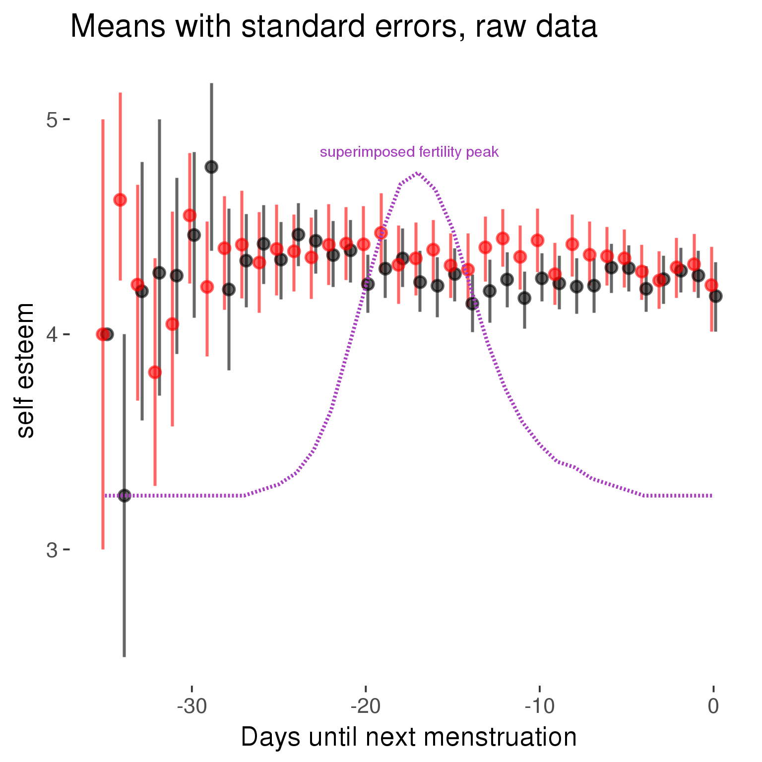
Forward-counted
model %>%
plot_curve(diary %>% filter(minimum_cycle_length_diary <= 36, minimum_cycle_length_diary > 20) %>% mutate(RCD = FCD, fertile = prc_stirn_b_forward_counted), caption_x = "Days since last menstruation")outcome = names(model@frame)[1]
outcome_label = recode(str_replace_all(str_replace_all(str_replace_all(outcome, "_", " "), " pair", "-pair"), " 1", ""),
"desirability 1" = "self-perceived desirability",
"NARQ admiration" = "narcissistic admiration",
"NARQ rivalry" = "narcissistic rivalry",
"extra-pair" = "extra-pair desire & behaviour",
"had sexual intercourse" = "sexual intercourse")
library(ggplot2)
# form a subset and run the model without the hormonal contraception and the fertility predictors
tmp = diary %>%
filter(!is.na(fertile), !is.na(included),
RCD > -1 * minimum_cycle_length_diary, RCD > -40)
new_form = update.formula(formula(model), new = . ~ . - fertile * included)
tmp$residuals = residuals(update(model, new_form, data = tmp , na.action = na.exclude))
tmp = tmp %>%
filter(!is.na(RCD), !is.na(residuals))
rcd_min = min(tmp$RCD)
tmp$real = FALSE
tmp_before = tmp
tmp_before$RCD = tmp_before$RCD + min(tmp$RCD) - 1
tmp_after = tmp
tmp_after$RCD = tmp_after$RCD - min(tmp$RCD) + 1
tmp$real = TRUE
tmp = bind_rows(tmp_before %>% filter(RCD > rcd_min - 11), tmp, tmp_after %>% filter(RCD < 11))GAM smooth on residuals
Here, we partialled out menstruation and individual random effects, then superimposed estimated probability of being in the fertile window scaled to the range of the estimated means. To address the periodicity of the cycle, we prepended and appended ten days of the timeseries to the end and the beginning of the timeseries. We then estimated the GAM and cut off the appended subsets before plotting.
tryCatch({
trend_plot = ggplot(tmp,aes(x = RCD, y = residuals, colour = included)) +
stat_smooth(geom = 'smooth',size = 0.8, fill = "#9ECAE1", method = 'gam', formula = y ~ s(x))
}, error = function(e){cat_message(e, "danger")})
tryCatch({
trend_data = ggplot_build(trend_plot)$data[[1]]
}, error = function(e){cat_message(e, "danger")})
trend_data$RCD = round(trend_data$x)
trend_data = left_join(trend_data, tmp %>% select(real, RCD,fertile) %>% unique(), by = "RCD")
trend_data %>%
filter(real == TRUE) %>%
mutate(superimposed = ( ( (fertile - 0.01)/0.58) * (max(y)-min(y) ) ) + min(y) ) ->
trend_data
ggplot(trend_data) +
geom_ribbon(aes(x = x, ymin = ymin, ymax = ymax, fill = factor(group)), alpha = 0.2) +
geom_line(aes(x = x, y = y, colour = factor(group)), size = 0.8, stat = "identity") +
scale_x_continuous(caption_x) +
geom_line(aes(x = x, y = superimposed), color = "#a83fbf", size = 1, linetype = 'dashed') +
annotate("text",x = mean(trend_data$x), y = max(trend_data$superimposed,na.rm=T) + 0.1, label = 'superimposed fertility peak', color = "#a83fbf") +
scale_y_continuous(outcome_label) +
ggtitle("GAM smooth, residuals") +
scale_color_manual("Contraception status",values = c("2"="black","1"= "red"), labels = c("2"="hormonally\ncontracepting","1"="cycling"), guide = F) +
scale_fill_manual("Contraception status",values = c("2"="black","1"= "red"), labels = c("2"="hormonally\ncontracepting","1"="cycling"), guide = F)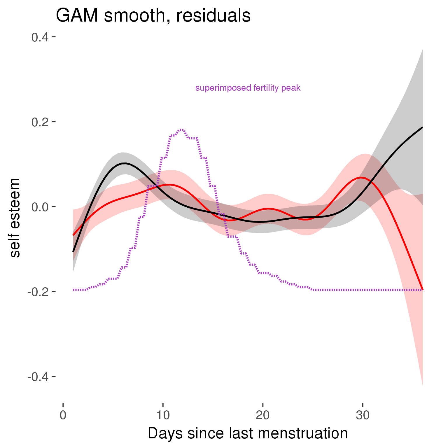
GAM smooth on raw data
As before, but without partialling anything out.
tryCatch({
trend_plot = ggplot(tmp,aes_string(x = "RCD", y = outcome, colour = "included")) +
stat_smooth(geom = 'smooth',size = 0.8, fill = "#9ECAE1", method = 'gam', formula = y ~ s(x))
}, error = function(e){cat_message(e, "danger")})
tryCatch({
trend_data = ggplot_build(trend_plot)$data[[1]]
}, error = function(e){cat_message(e, "danger")})
trend_data$RCD = round(trend_data$x)
trend_data = left_join(trend_data, tmp %>% select(real, RCD,fertile) %>% unique(), by = "RCD")
trend_data %>%
filter(real == TRUE) %>%
mutate(superimposed = ( ( (fertile - 0.01)/0.58) * (max(y)-min(y) ) ) + min(y) ) ->
trend_data
plot1b = ggplot(trend_data) +
geom_ribbon(aes(x = x, ymin = ymin, ymax = ymax, fill = factor(group)), alpha = 0.2) +
geom_line(aes(x = x, y = y, colour = factor(group)), size = 0.8, stat = "identity") +
scale_x_continuous(caption_x) +
geom_line(aes(x = x, y = superimposed), color = "#a83fbf", size = 1, linetype = 'dashed') +
annotate("text",x = mean(trend_data$x), y = max(trend_data$superimposed,na.rm=T) + 0.1, label = 'superimposed fertility peak', color = "#a83fbf") +
scale_y_continuous(outcome_label) +
ggtitle("GAM smooth, raw data") +
scale_color_manual("Contraception status",values = c("2"="black","1"= "red"), labels = c("2"="hormonally\ncontracepting","1"="cycling"), guide = F) +
scale_fill_manual("Contraception status",values = c("2"="black","1"= "red"), labels = c("2"="hormonally\ncontracepting","1"="cycling"), guide = F)
suppressWarnings(print(plot1b))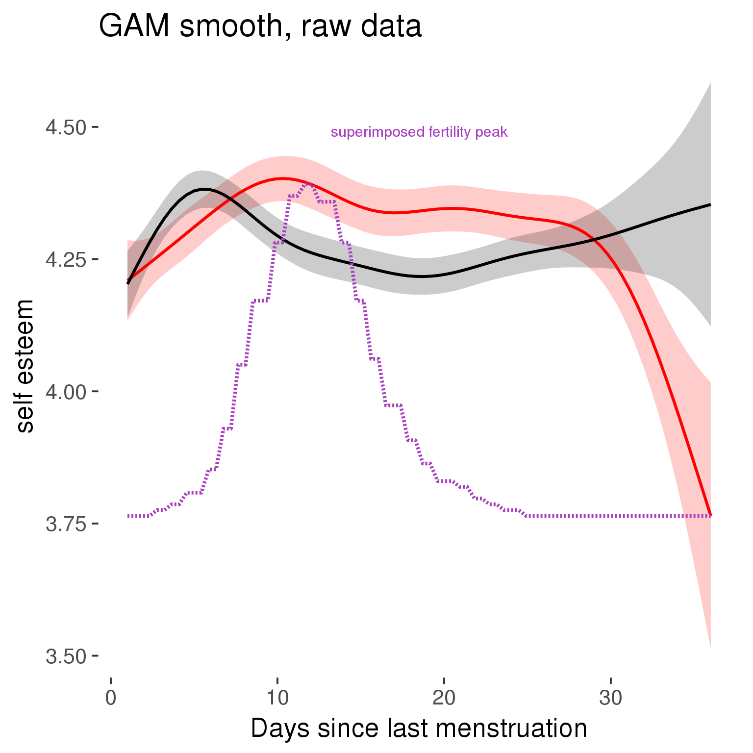
Means and standard errors over raw data
Nothing partialled out, just straight means with bootstrapped confidence intervals.
tryCatch({
trend_plot = ggplot(tmp,aes_string(x = "RCD", y = outcome, colour = "included")) +
geom_pointrange(size = 0.8, stat = 'summary', fun.data = "mean_cl_boot")
}, error = function(e){cat_message(e, "danger")})
tryCatch({
trend_data = ggplot_build(trend_plot)$data[[1]]
}, error = function(e){cat_message(e, "danger")})
trend_data$RCD = round(trend_data$x)
trend_data = left_join(trend_data, tmp %>% select(real, RCD,fertile) %>% unique(), by = "RCD")
trend_data %>%
filter(real == TRUE) %>%
mutate(superimposed = ( ( (fertile - 0.01)/0.58) * (max(y)-min(y) ) ) + min(y) ) ->
trend_data
plot3 = ggplot(trend_data) +
geom_pointrange(aes(x = x, y = y, ymin = ymin,ymax = ymax, colour = factor(group)), size = 0.8, stat = "identity", alpha = 0.6, position = position_dodge(width = .5)) +
scale_x_continuous("Days until next menstruation") +
geom_line(aes(x= x, y = superimposed), color = "#a83fbf", size = 1, linetype = 'dashed') +
annotate("text",x = mean(trend_data$x), y = max(trend_data$superimposed,na.rm=T) + 0.1, label = 'superimposed fertility peak', color = "#a83fbf") +
scale_y_continuous(outcome_label) +
ggtitle("Means with standard errors, raw data") +
scale_color_manual("Contraception status",values = c("2"="black","1"= "red"), labels = c("2"="hormonally\ncontracepting","1"="cycling"), guide = F) +
scale_fill_manual("Contraception status",values = c("2"="black","1"= "red"), labels = c("2"="hormonally\ncontracepting","1"="cycling"), guide = F)
suppressWarnings(print(plot3))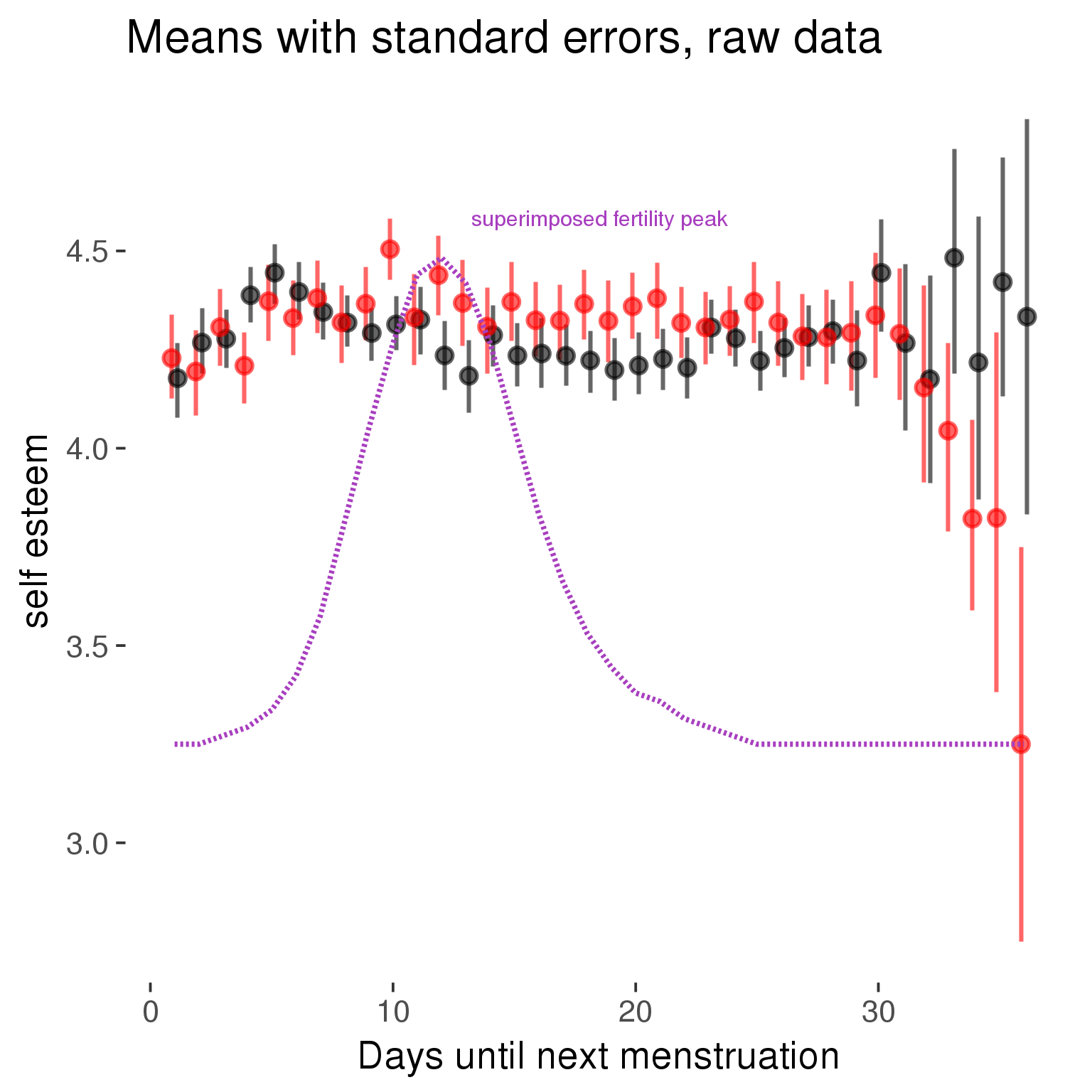
Cycle lengths from 27 to 30
Backward-counted
model %>%
plot_curve(diary %>% filter(minimum_cycle_length_diary <= 30, minimum_cycle_length_diary >= 27) %>% mutate(fertile=prc_stirn_b))outcome = names(model@frame)[1]
outcome_label = recode(str_replace_all(str_replace_all(str_replace_all(outcome, "_", " "), " pair", "-pair"), " 1", ""),
"desirability 1" = "self-perceived desirability",
"NARQ admiration" = "narcissistic admiration",
"NARQ rivalry" = "narcissistic rivalry",
"extra-pair" = "extra-pair desire & behaviour",
"had sexual intercourse" = "sexual intercourse")
library(ggplot2)
# form a subset and run the model without the hormonal contraception and the fertility predictors
tmp = diary %>%
filter(!is.na(fertile), !is.na(included),
RCD > -1 * minimum_cycle_length_diary, RCD > -40)
new_form = update.formula(formula(model), new = . ~ . - fertile * included)
tmp$residuals = residuals(update(model, new_form, data = tmp , na.action = na.exclude))
tmp = tmp %>%
filter(!is.na(RCD), !is.na(residuals))
rcd_min = min(tmp$RCD)
tmp$real = FALSE
tmp_before = tmp
tmp_before$RCD = tmp_before$RCD + min(tmp$RCD) - 1
tmp_after = tmp
tmp_after$RCD = tmp_after$RCD - min(tmp$RCD) + 1
tmp$real = TRUE
tmp = bind_rows(tmp_before %>% filter(RCD > rcd_min - 11), tmp, tmp_after %>% filter(RCD < 11))GAM smooth on residuals
Here, we partialled out menstruation and individual random effects, then superimposed estimated probability of being in the fertile window scaled to the range of the estimated means. To address the periodicity of the cycle, we prepended and appended ten days of the timeseries to the end and the beginning of the timeseries. We then estimated the GAM and cut off the appended subsets before plotting.
tryCatch({
trend_plot = ggplot(tmp,aes(x = RCD, y = residuals, colour = included)) +
stat_smooth(geom = 'smooth',size = 0.8, fill = "#9ECAE1", method = 'gam', formula = y ~ s(x))
}, error = function(e){cat_message(e, "danger")})
tryCatch({
trend_data = ggplot_build(trend_plot)$data[[1]]
}, error = function(e){cat_message(e, "danger")})
trend_data$RCD = round(trend_data$x)
trend_data = left_join(trend_data, tmp %>% select(real, RCD,fertile) %>% unique(), by = "RCD")
trend_data %>%
filter(real == TRUE) %>%
mutate(superimposed = ( ( (fertile - 0.01)/0.58) * (max(y)-min(y) ) ) + min(y) ) ->
trend_data
ggplot(trend_data) +
geom_ribbon(aes(x = x, ymin = ymin, ymax = ymax, fill = factor(group)), alpha = 0.2) +
geom_line(aes(x = x, y = y, colour = factor(group)), size = 0.8, stat = "identity") +
scale_x_continuous(caption_x) +
geom_line(aes(x = x, y = superimposed), color = "#a83fbf", size = 1, linetype = 'dashed') +
annotate("text",x = mean(trend_data$x), y = max(trend_data$superimposed,na.rm=T) + 0.1, label = 'superimposed fertility peak', color = "#a83fbf") +
scale_y_continuous(outcome_label) +
ggtitle("GAM smooth, residuals") +
scale_color_manual("Contraception status",values = c("2"="black","1"= "red"), labels = c("2"="hormonally\ncontracepting","1"="cycling"), guide = F) +
scale_fill_manual("Contraception status",values = c("2"="black","1"= "red"), labels = c("2"="hormonally\ncontracepting","1"="cycling"), guide = F)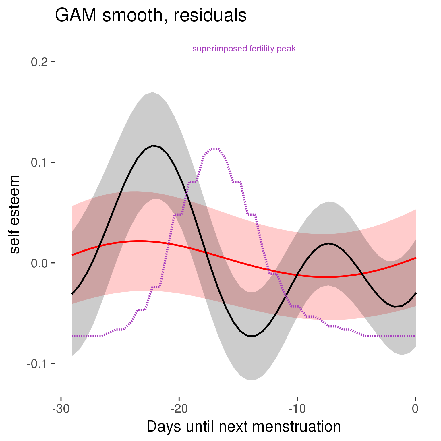
GAM smooth on raw data
As before, but without partialling anything out.
tryCatch({
trend_plot = ggplot(tmp,aes_string(x = "RCD", y = outcome, colour = "included")) +
stat_smooth(geom = 'smooth',size = 0.8, fill = "#9ECAE1", method = 'gam', formula = y ~ s(x))
}, error = function(e){cat_message(e, "danger")})
tryCatch({
trend_data = ggplot_build(trend_plot)$data[[1]]
}, error = function(e){cat_message(e, "danger")})
trend_data$RCD = round(trend_data$x)
trend_data = left_join(trend_data, tmp %>% select(real, RCD,fertile) %>% unique(), by = "RCD")
trend_data %>%
filter(real == TRUE) %>%
mutate(superimposed = ( ( (fertile - 0.01)/0.58) * (max(y)-min(y) ) ) + min(y) ) ->
trend_data
plot1b = ggplot(trend_data) +
geom_ribbon(aes(x = x, ymin = ymin, ymax = ymax, fill = factor(group)), alpha = 0.2) +
geom_line(aes(x = x, y = y, colour = factor(group)), size = 0.8, stat = "identity") +
scale_x_continuous(caption_x) +
geom_line(aes(x = x, y = superimposed), color = "#a83fbf", size = 1, linetype = 'dashed') +
annotate("text",x = mean(trend_data$x), y = max(trend_data$superimposed,na.rm=T) + 0.1, label = 'superimposed fertility peak', color = "#a83fbf") +
scale_y_continuous(outcome_label) +
ggtitle("GAM smooth, raw data") +
scale_color_manual("Contraception status",values = c("2"="black","1"= "red"), labels = c("2"="hormonally\ncontracepting","1"="cycling"), guide = F) +
scale_fill_manual("Contraception status",values = c("2"="black","1"= "red"), labels = c("2"="hormonally\ncontracepting","1"="cycling"), guide = F)
suppressWarnings(print(plot1b))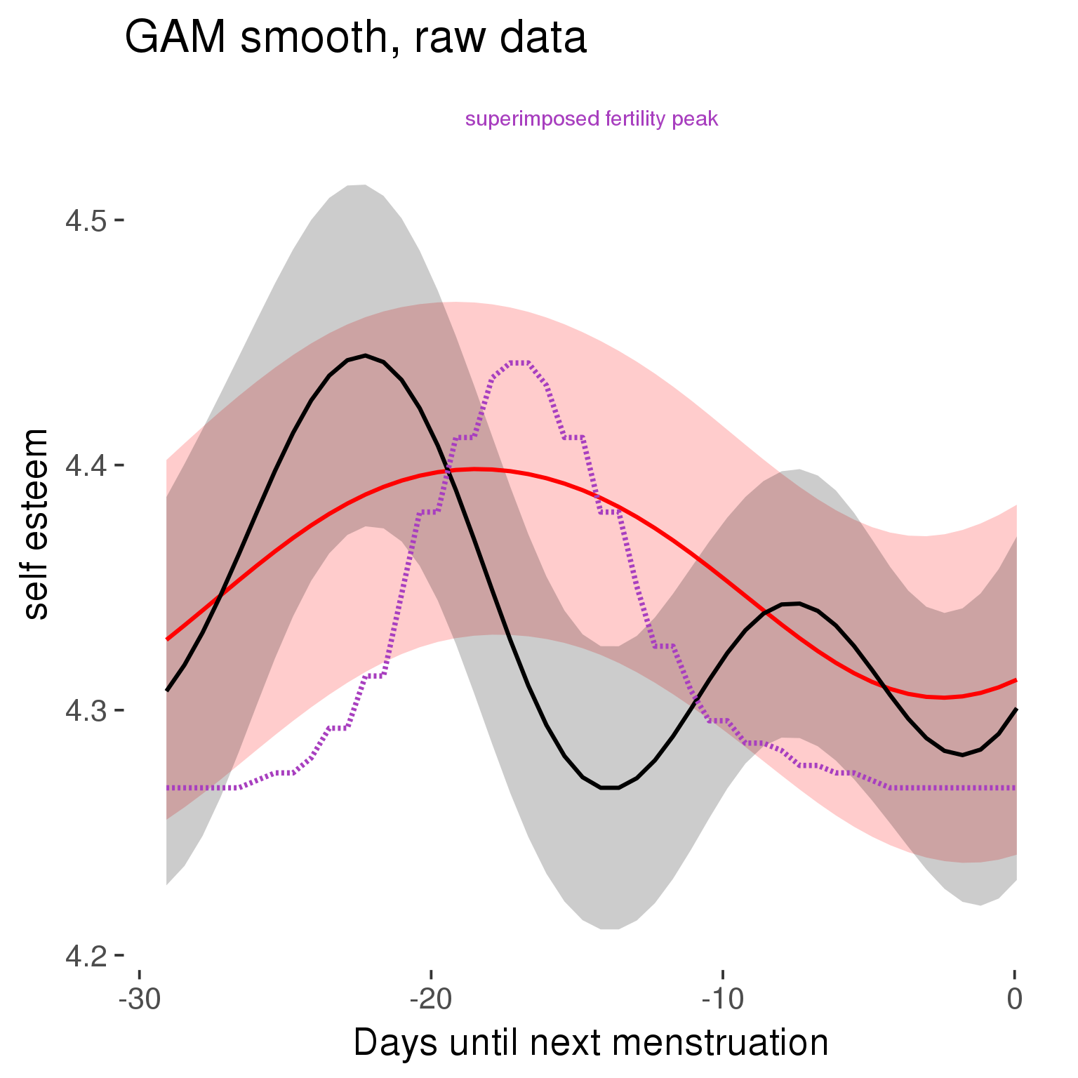
Means and standard errors over raw data
Nothing partialled out, just straight means with bootstrapped confidence intervals.
tryCatch({
trend_plot = ggplot(tmp,aes_string(x = "RCD", y = outcome, colour = "included")) +
geom_pointrange(size = 0.8, stat = 'summary', fun.data = "mean_cl_boot")
}, error = function(e){cat_message(e, "danger")})
tryCatch({
trend_data = ggplot_build(trend_plot)$data[[1]]
}, error = function(e){cat_message(e, "danger")})
trend_data$RCD = round(trend_data$x)
trend_data = left_join(trend_data, tmp %>% select(real, RCD,fertile) %>% unique(), by = "RCD")
trend_data %>%
filter(real == TRUE) %>%
mutate(superimposed = ( ( (fertile - 0.01)/0.58) * (max(y)-min(y) ) ) + min(y) ) ->
trend_data
plot3 = ggplot(trend_data) +
geom_pointrange(aes(x = x, y = y, ymin = ymin,ymax = ymax, colour = factor(group)), size = 0.8, stat = "identity", alpha = 0.6, position = position_dodge(width = .5)) +
scale_x_continuous("Days until next menstruation") +
geom_line(aes(x= x, y = superimposed), color = "#a83fbf", size = 1, linetype = 'dashed') +
annotate("text",x = mean(trend_data$x), y = max(trend_data$superimposed,na.rm=T) + 0.1, label = 'superimposed fertility peak', color = "#a83fbf") +
scale_y_continuous(outcome_label) +
ggtitle("Means with standard errors, raw data") +
scale_color_manual("Contraception status",values = c("2"="black","1"= "red"), labels = c("2"="hormonally\ncontracepting","1"="cycling"), guide = F) +
scale_fill_manual("Contraception status",values = c("2"="black","1"= "red"), labels = c("2"="hormonally\ncontracepting","1"="cycling"), guide = F)
suppressWarnings(print(plot3))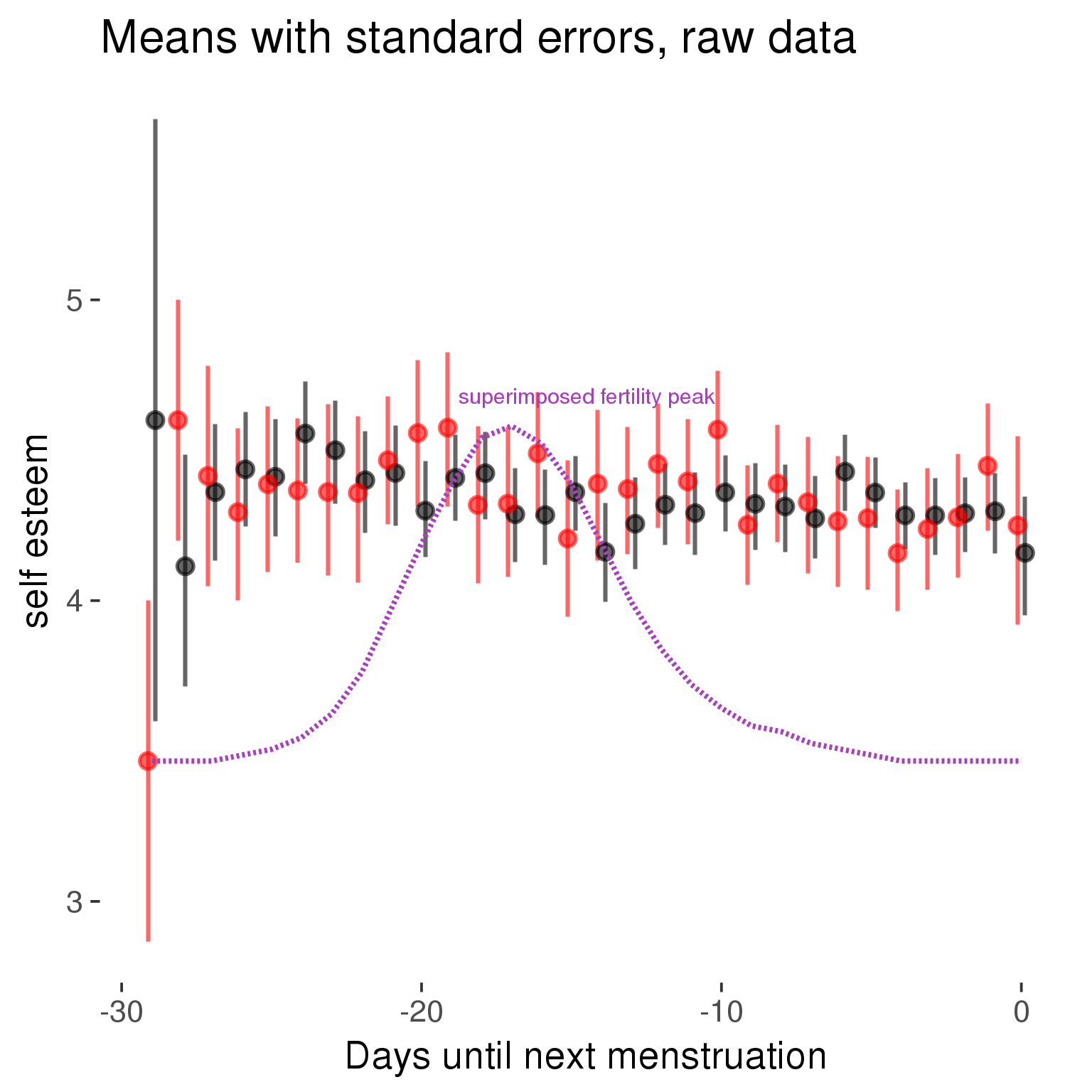
Forward-counted
model %>%
plot_curve(diary %>% filter(minimum_cycle_length_diary <= 30, minimum_cycle_length_diary >= 27) %>% mutate(RCD = FCD, fertile = prc_stirn_b_forward_counted), caption_x = "Days since last menstruation")outcome = names(model@frame)[1]
outcome_label = recode(str_replace_all(str_replace_all(str_replace_all(outcome, "_", " "), " pair", "-pair"), " 1", ""),
"desirability 1" = "self-perceived desirability",
"NARQ admiration" = "narcissistic admiration",
"NARQ rivalry" = "narcissistic rivalry",
"extra-pair" = "extra-pair desire & behaviour",
"had sexual intercourse" = "sexual intercourse")
library(ggplot2)
# form a subset and run the model without the hormonal contraception and the fertility predictors
tmp = diary %>%
filter(!is.na(fertile), !is.na(included),
RCD > -1 * minimum_cycle_length_diary, RCD > -40)
new_form = update.formula(formula(model), new = . ~ . - fertile * included)
tmp$residuals = residuals(update(model, new_form, data = tmp , na.action = na.exclude))
tmp = tmp %>%
filter(!is.na(RCD), !is.na(residuals))
rcd_min = min(tmp$RCD)
tmp$real = FALSE
tmp_before = tmp
tmp_before$RCD = tmp_before$RCD + min(tmp$RCD) - 1
tmp_after = tmp
tmp_after$RCD = tmp_after$RCD - min(tmp$RCD) + 1
tmp$real = TRUE
tmp = bind_rows(tmp_before %>% filter(RCD > rcd_min - 11), tmp, tmp_after %>% filter(RCD < 11))GAM smooth on residuals
Here, we partialled out menstruation and individual random effects, then superimposed estimated probability of being in the fertile window scaled to the range of the estimated means. To address the periodicity of the cycle, we prepended and appended ten days of the timeseries to the end and the beginning of the timeseries. We then estimated the GAM and cut off the appended subsets before plotting.
tryCatch({
trend_plot = ggplot(tmp,aes(x = RCD, y = residuals, colour = included)) +
stat_smooth(geom = 'smooth',size = 0.8, fill = "#9ECAE1", method = 'gam', formula = y ~ s(x))
}, error = function(e){cat_message(e, "danger")})
tryCatch({
trend_data = ggplot_build(trend_plot)$data[[1]]
}, error = function(e){cat_message(e, "danger")})
trend_data$RCD = round(trend_data$x)
trend_data = left_join(trend_data, tmp %>% select(real, RCD,fertile) %>% unique(), by = "RCD")
trend_data %>%
filter(real == TRUE) %>%
mutate(superimposed = ( ( (fertile - 0.01)/0.58) * (max(y)-min(y) ) ) + min(y) ) ->
trend_data
ggplot(trend_data) +
geom_ribbon(aes(x = x, ymin = ymin, ymax = ymax, fill = factor(group)), alpha = 0.2) +
geom_line(aes(x = x, y = y, colour = factor(group)), size = 0.8, stat = "identity") +
scale_x_continuous(caption_x) +
geom_line(aes(x = x, y = superimposed), color = "#a83fbf", size = 1, linetype = 'dashed') +
annotate("text",x = mean(trend_data$x), y = max(trend_data$superimposed,na.rm=T) + 0.1, label = 'superimposed fertility peak', color = "#a83fbf") +
scale_y_continuous(outcome_label) +
ggtitle("GAM smooth, residuals") +
scale_color_manual("Contraception status",values = c("2"="black","1"= "red"), labels = c("2"="hormonally\ncontracepting","1"="cycling"), guide = F) +
scale_fill_manual("Contraception status",values = c("2"="black","1"= "red"), labels = c("2"="hormonally\ncontracepting","1"="cycling"), guide = F)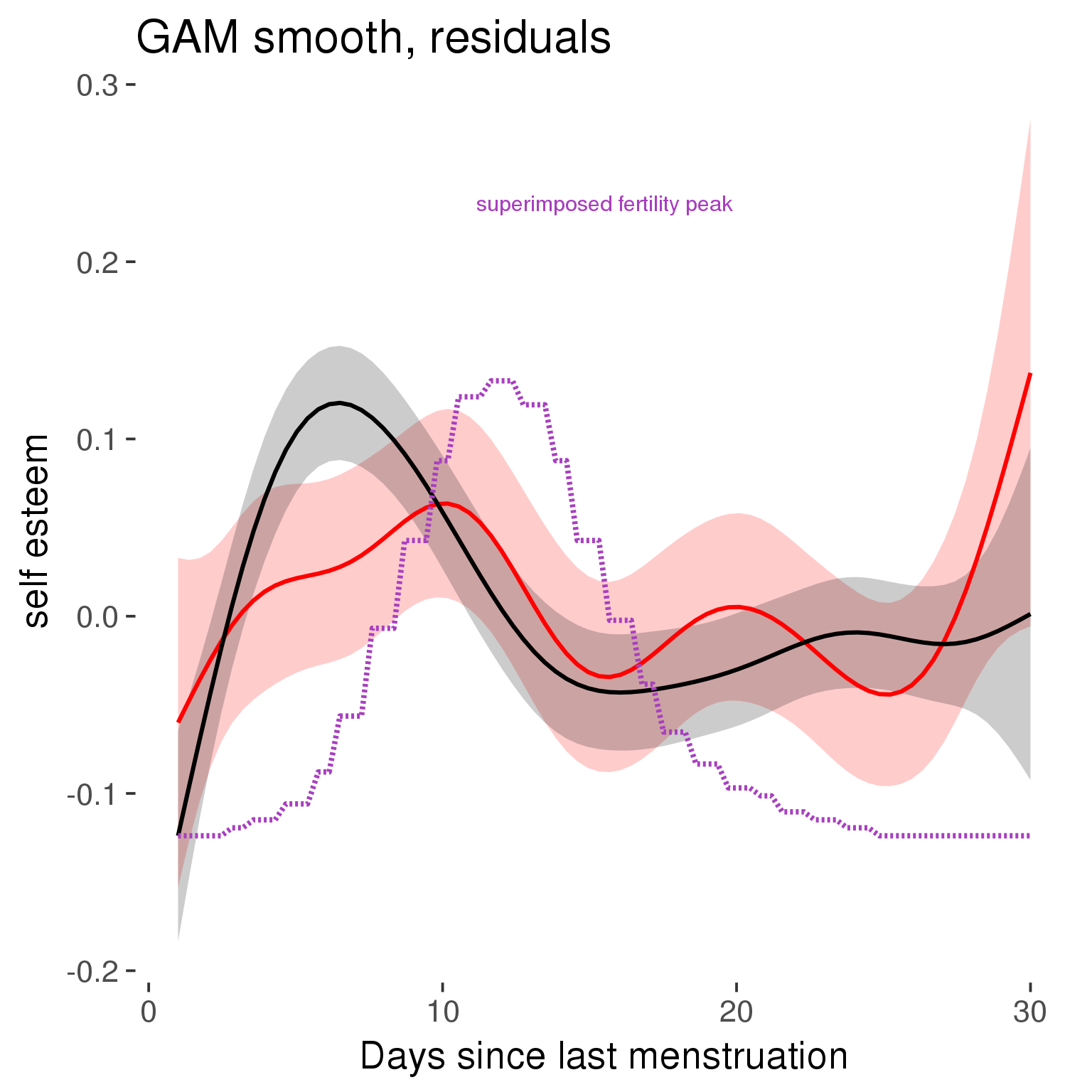
GAM smooth on raw data
As before, but without partialling anything out.
tryCatch({
trend_plot = ggplot(tmp,aes_string(x = "RCD", y = outcome, colour = "included")) +
stat_smooth(geom = 'smooth',size = 0.8, fill = "#9ECAE1", method = 'gam', formula = y ~ s(x))
}, error = function(e){cat_message(e, "danger")})
tryCatch({
trend_data = ggplot_build(trend_plot)$data[[1]]
}, error = function(e){cat_message(e, "danger")})
trend_data$RCD = round(trend_data$x)
trend_data = left_join(trend_data, tmp %>% select(real, RCD,fertile) %>% unique(), by = "RCD")
trend_data %>%
filter(real == TRUE) %>%
mutate(superimposed = ( ( (fertile - 0.01)/0.58) * (max(y)-min(y) ) ) + min(y) ) ->
trend_data
plot1b = ggplot(trend_data) +
geom_ribbon(aes(x = x, ymin = ymin, ymax = ymax, fill = factor(group)), alpha = 0.2) +
geom_line(aes(x = x, y = y, colour = factor(group)), size = 0.8, stat = "identity") +
scale_x_continuous(caption_x) +
geom_line(aes(x = x, y = superimposed), color = "#a83fbf", size = 1, linetype = 'dashed') +
annotate("text",x = mean(trend_data$x), y = max(trend_data$superimposed,na.rm=T) + 0.1, label = 'superimposed fertility peak', color = "#a83fbf") +
scale_y_continuous(outcome_label) +
ggtitle("GAM smooth, raw data") +
scale_color_manual("Contraception status",values = c("2"="black","1"= "red"), labels = c("2"="hormonally\ncontracepting","1"="cycling"), guide = F) +
scale_fill_manual("Contraception status",values = c("2"="black","1"= "red"), labels = c("2"="hormonally\ncontracepting","1"="cycling"), guide = F)
suppressWarnings(print(plot1b))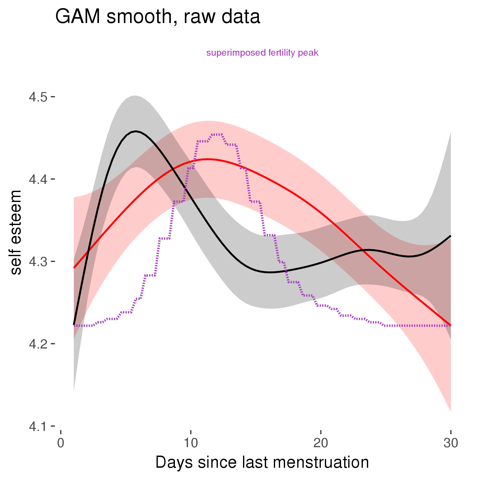
Means and standard errors over raw data
Nothing partialled out, just straight means with bootstrapped confidence intervals.
tryCatch({
trend_plot = ggplot(tmp,aes_string(x = "RCD", y = outcome, colour = "included")) +
geom_pointrange(size = 0.8, stat = 'summary', fun.data = "mean_cl_boot")
}, error = function(e){cat_message(e, "danger")})
tryCatch({
trend_data = ggplot_build(trend_plot)$data[[1]]
}, error = function(e){cat_message(e, "danger")})
trend_data$RCD = round(trend_data$x)
trend_data = left_join(trend_data, tmp %>% select(real, RCD,fertile) %>% unique(), by = "RCD")
trend_data %>%
filter(real == TRUE) %>%
mutate(superimposed = ( ( (fertile - 0.01)/0.58) * (max(y)-min(y) ) ) + min(y) ) ->
trend_data
plot3 = ggplot(trend_data) +
geom_pointrange(aes(x = x, y = y, ymin = ymin,ymax = ymax, colour = factor(group)), size = 0.8, stat = "identity", alpha = 0.6, position = position_dodge(width = .5)) +
scale_x_continuous("Days until next menstruation") +
geom_line(aes(x= x, y = superimposed), color = "#a83fbf", size = 1, linetype = 'dashed') +
annotate("text",x = mean(trend_data$x), y = max(trend_data$superimposed,na.rm=T) + 0.1, label = 'superimposed fertility peak', color = "#a83fbf") +
scale_y_continuous(outcome_label) +
ggtitle("Means with standard errors, raw data") +
scale_color_manual("Contraception status",values = c("2"="black","1"= "red"), labels = c("2"="hormonally\ncontracepting","1"="cycling"), guide = F) +
scale_fill_manual("Contraception status",values = c("2"="black","1"= "red"), labels = c("2"="hormonally\ncontracepting","1"="cycling"), guide = F)
suppressWarnings(print(plot3))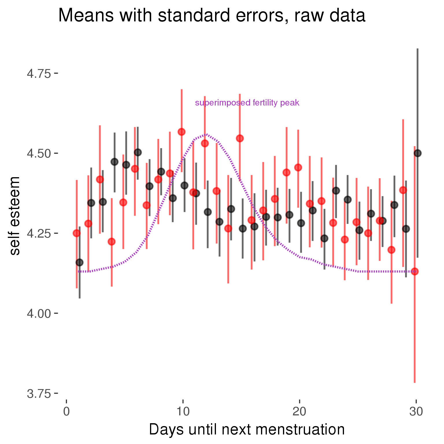
Robustness checks
M_r1: Random slopes for conception risk and menstruation
tryCatch({
# refit model with random effects for fertile and menstruation dummies
with_ind_diff = update(model, formula = . ~ . - (1| person) + (1 + fertile + menstruation | person))
# pull the random effects, format as tibble
rand = coef(with_ind_diff)$person %>%
tibble::rownames_to_column("person") %>%
mutate(person = as.numeric(person))
# pull the fixed effects
fixd = data.frame(fixef(with_ind_diff)) %>%
tibble::rownames_to_column("effect")
names(fixd) = c("effect", "pop_effect_size")
# pull apart the coefficients so that we can account for the fact that the random effect variation implicitly includes HC explaining the mean population-level effect of fertile/menstruation dummies among HC users
fixd = fixd %>%
separate(effect, c("included", "effect"), sep = ":", fill = "left") %>%
mutate(included = if_else(is.na(included), "cycling", str_replace(included, "included", "")))
fixd[2,c("included", "effect")] = c("horm_contra", "(Intercept)")
rand = rand %>%
# merge diary data on the random effects, so that we know who is a HC users and who isn't
inner_join(diary %>% select(person, included) %>% unique(), by = 'person') %>%
# gather into long format, to have the dataset by predictor
gather(effect, value, -person, -included) %>%
inner_join(fixd, by = c('effect', 'included')) %>%
# pull the fixed effects
mutate(
# only for those who are HC users, add the moderated population effect size for this effect (the random effects have the reference category mean)
value = if_else(included == "horm_contra", value + pop_effect_size, value),
effect = recode(effect, "includedhorm_contra" = "HC user",
"includedhorm_contra:fertile" = "HC user x fertile",
"includedhorm_contra:menstruationpre" = "HC user x premens.",
"includedhorm_contra:menstruationyes" = "HC user x mens.",
"menstruationyes" = "mens.",
"menstruationpre" = "premens.")) %>%
group_by(included, effect) %>%
# filter out predictors that aren't modelled as varying/random
filter(sd(value) > 0)
# plot dot plot of random effects
print(
ggplot(rand, aes(x = included, y = value, color = included, fill = included)) +
facet_wrap( ~ effect, scales = "free") +
# geom_violin(alpha = 0.4, size = 0) +
geom_dotplot(binaxis='y', dotsize = 0.1, method = "histodot") +
# geom_jitter(alpha = 0.05) +
coord_flip() +
geom_pointrange(stat = 'summary', fun.data = 'mean_sdl', color = 'darkred', size = 1.2) +
scale_color_manual("Contraception status", values = c("horm_contra"="black","cycling"= "red"), labels = c("horm_contra"="hormonally\ncontracepting","cycling"="cycling"), guide = F) +
scale_fill_manual("Contraception status", values = c("horm_contra"="black","cycling"= "red"), labels = c("horm_contra"="hormonally\ncontracepting","1"="cycling"), guide = F) +
ggtitle("M_r1: allowing participant-varying slopes", subtitle = "for the conception risk measure and the menstruation dummies") +
scale_x_discrete("Hormonal contraception", breaks = c("horm_contra", "cycling"), labels = c("yes", "no")) +
scale_y_continuous("Random effect size distribution"))
print_summary(with_ind_diff)
cat(pander(anova(model, with_ind_diff)))
}, error = function(e){
with_ind_diff = model
cat_message(e, "danger")
})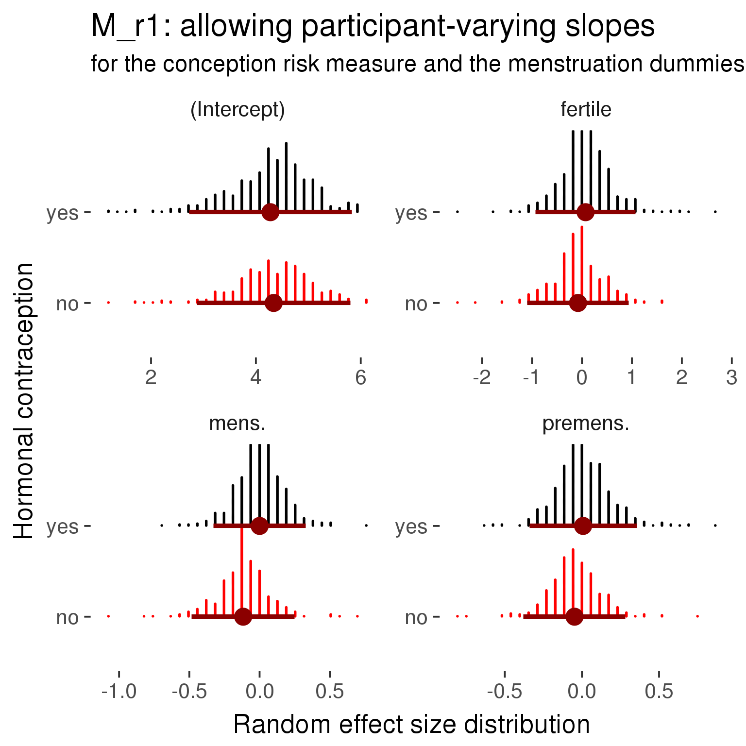
Linear mixed model fit by REML ['lmerMod']
Formula: self_esteem_1 ~ included + menstruation + fertile + fertile_mean +
(1 + fertile + menstruation | person) + included:menstruation + included:fertile
Data: diary
REML criterion at convergence: 72146
Scaled residuals:
Min 1Q Median 3Q Max
-5.244 -0.490 0.098 0.615 3.819
Random effects:
Groups Name Variance Std.Dev. Corr
person (Intercept) 0.670 0.819
fertile 0.720 0.849 -0.33
menstruationpre 0.108 0.328 -0.33 0.46
menstruationyes 0.111 0.333 -0.21 0.30 0.63
Residual 0.751 0.866
Number of obs: 26685, groups: person, 1054
Fixed effects:
Estimate Std. Error t value
(Intercept) 4.3392 0.0680 63.8
includedhorm_contra -0.0617 0.0576 -1.1
menstruationpre -0.0481 0.0326 -1.5
menstruationyes -0.1167 0.0316 -3.7
fertile -0.0783 0.0721 -1.1
fertile_mean -0.2162 0.3063 -0.7
includedhorm_contra:menstruationpre 0.0556 0.0419 1.3
includedhorm_contra:menstruationyes 0.1171 0.0411 2.8
includedhorm_contra:fertile 0.1513 0.0916 1.7
Correlation of Fixed Effects:
(Intr) incld_ mnstrtnp mnstrtny fertil frtl_m inclddhrm_cntr:mnstrtnp
inclddhrm_c -0.491
menstrutnpr -0.238 0.284
menstrutnys -0.197 0.236 0.470
fertile -0.221 0.332 0.451 0.348
fertile_men -0.754 -0.025 -0.004 -0.003 -0.078
inclddhrm_cntr:mnstrtnp 0.193 -0.361 -0.779 -0.366 -0.350 -0.007
inclddhrm_cntr:mnstrtny 0.157 -0.294 -0.361 -0.768 -0.266 -0.005 0.460
inclddhrm_cntr:f 0.212 -0.423 -0.355 -0.274 -0.783 0.011 0.451
inclddhrm_cntr:mnstrtny
inclddhrm_c
menstrutnpr
menstrutnys
fertile
fertile_men
inclddhrm_cntr:mnstrtnp
inclddhrm_cntr:mnstrtny
inclddhrm_cntr:f 0.344
refitting model(s) with ML (instead of REML)
| Df | AIC | BIC | logLik | deviance | Chisq | Chi Df | Pr(>Chisq) | |
|---|---|---|---|---|---|---|---|---|
| object | 11 | 72452 | 72542 | -36215 | 72430 | NA | NA | NA |
| ..1 | 20 | 72147 | 72311 | -36054 | 72107 | 322.8 | 9 | 3.704e-64 |
robustness_check_ovu_shift(model, diary)M_e: Exclusion criteria
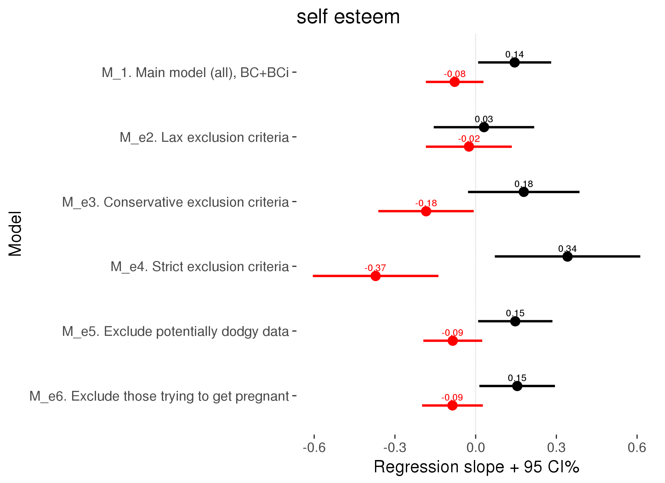
M_p: Predictors
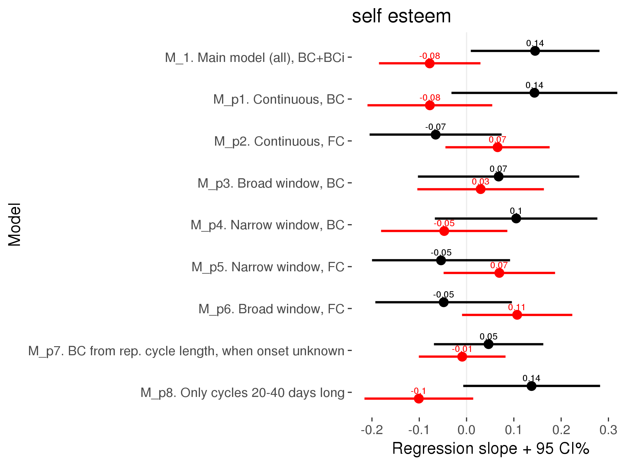
M_c: Covariates, controls, autocorrelation
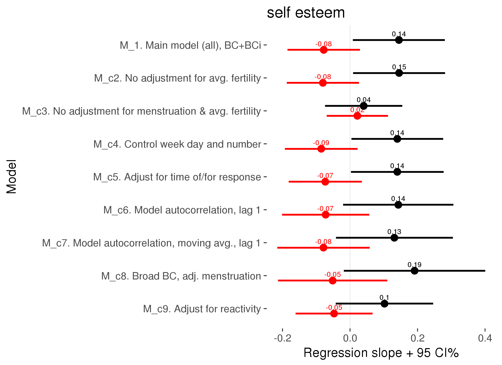
Linear mixed model fit by REML ['lmerMod']
REML criterion at convergence: 66093
Scaled residuals:
Min 1Q Median 3Q Max
-5.306 -0.498 0.096 0.630 4.250
Random effects:
Groups Name Variance Std.Dev.
person (Intercept) 5.86e-01 0.7656010473
Xr.2 s(days_filled_out):includedhorm_contra 8.39e-04 0.0289688959
Xr.1 s(days_filled_out):includedcycling 5.10e-03 0.0714176477
Xr.0 s(day_number):includedhorm_contra 0.00e+00 0.0000000000
Xr s(day_number):includedcycling 3.20e-15 0.0000000566
Residual 7.83e-01 0.8847480492
Number of obs: 24382, groups: person, 1054; Xr.2, 8; Xr.1, 8; Xr.0, 8; Xr, 8
Fixed effects:
Estimate Std. Error t value
X(Intercept) 4.3282 0.0666 65.0
Xincludedhorm_contra -0.0589 0.0549 -1.1
Xmenstruationpre -0.0553 0.0282 -2.0
Xmenstruationyes -0.1088 0.0271 -4.0
Xfertile -0.0473 0.0581 -0.8
Xfertile_mean -0.1692 0.3032 -0.6
Xincludedhorm_contra:menstruationpre 0.0539 0.0362 1.5
Xincludedhorm_contra:menstruationyes 0.1086 0.0355 3.1
Xincludedhorm_contra:fertile 0.1021 0.0736 1.4
Xs(day_number):includedcyclingFx1 -0.0752 0.0462 -1.6
Xs(day_number):includedhorm_contraFx1 0.0169 0.0391 0.4
Xs(days_filled_out):includedcyclingFx1 0.0638 0.0543 1.2
Xs(days_filled_out):includedhorm_contraFx1 -0.0579 0.0415 -1.4
Family: gaussian
Link function: identity
Formula:
self_esteem_1 ~ included + menstruation + fertile + fertile_mean +
s(day_number, by = included) + s(days_filled_out, by = included) +
included:menstruation + included:fertile
Parametric coefficients:
Estimate Std. Error t value Pr(>|t|)
(Intercept) 4.3282 0.0666 65.04 < 2e-16 ***
includedhorm_contra -0.0589 0.0549 -1.07 0.2842
menstruationpre -0.0553 0.0282 -1.96 0.0502 .
menstruationyes -0.1088 0.0271 -4.01 0.00006 ***
fertile -0.0473 0.0581 -0.81 0.4156
fertile_mean -0.1692 0.3032 -0.56 0.5767
includedhorm_contra:menstruationpre 0.0539 0.0362 1.49 0.1366
includedhorm_contra:menstruationyes 0.1086 0.0355 3.06 0.0022 **
includedhorm_contra:fertile 0.1021 0.0736 1.39 0.1651
---
Signif. codes: 0 '***' 0.001 '**' 0.01 '*' 0.05 '.' 0.1 ' ' 1
Approximate significance of smooth terms:
edf Ref.df F p-value
s(day_number):includedcycling 1.00 1.00 2.65 0.103
s(day_number):includedhorm_contra 1.00 1.00 0.19 0.666
s(days_filled_out):includedcycling 2.08 2.08 3.05 0.049 *
s(days_filled_out):includedhorm_contra 1.49 1.49 1.26 0.195
---
Signif. codes: 0 '***' 0.001 '**' 0.01 '*' 0.05 '.' 0.1 ' ' 1
R-sq.(adj) = 0.00134
lmer.REML = 66093 Scale est. = 0.78278 n = 24382
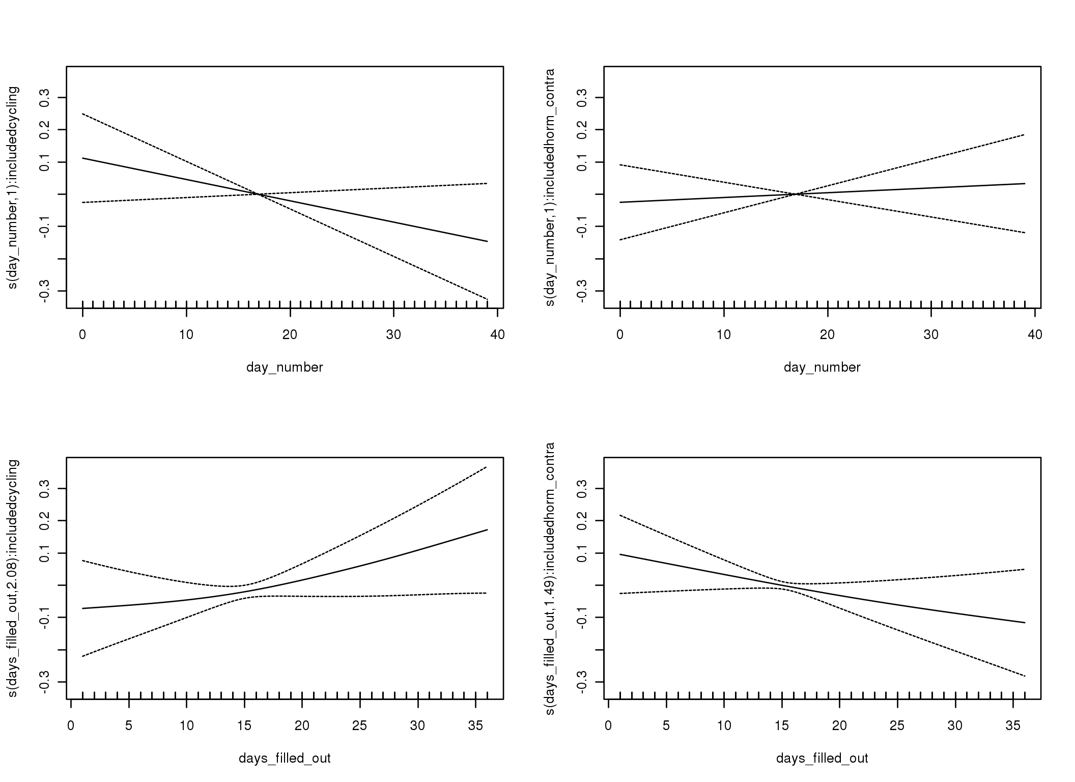
Linear mixed-effects model fit by REML
Data: diary
AIC BIC logLik
71084 71183 -35530
Random effects:
Formula: ~1 | person
(Intercept) Residual
StdDev: 0.7503 0.9014
Correlation Structure: ARMA(1,0)
Formula: ~day_number | person
Parameter estimate(s):
Phi1
0.2723
Fixed effects: self_esteem_1 ~ included * (menstruation + fertile) + fertile_mean
Value Std.Error DF t-value p-value
(Intercept) 4.339 0.06708 25625 64.68 0.0000
includedhorm_contra -0.057 0.05524 1051 -1.03 0.3017
menstruationpre -0.039 0.03120 25625 -1.26 0.2068
menstruationyes -0.117 0.02915 25625 -4.02 0.0001
fertile -0.072 0.06593 25625 -1.10 0.2728
fertile_mean -0.235 0.30749 1051 -0.76 0.4451
includedhorm_contra:menstruationpre 0.050 0.04008 25625 1.26 0.2083
includedhorm_contra:menstruationyes 0.123 0.03802 25625 3.24 0.0012
includedhorm_contra:fertile 0.143 0.08342 25625 1.72 0.0863
Correlation:
(Intr) incld_ mnstrtnp mnstrtny fertil frtl_m inclddhrm_cntr:mnstrtnp
includedhorm_contra -0.477
menstruationpre -0.177 0.222
menstruationyes -0.174 0.216 0.402
fertile -0.170 0.282 0.432 0.363
fertile_mean -0.769 -0.026 -0.008 -0.006 -0.078
includedhorm_contra:menstruationpre 0.146 -0.278 -0.779 -0.313 -0.335 -0.004
includedhorm_contra:menstruationyes 0.139 -0.265 -0.308 -0.767 -0.278 -0.003 0.387
includedhorm_contra:fertile 0.172 -0.356 -0.341 -0.287 -0.787 0.013 0.431
inclddhrm_cntr:mnstrtny
includedhorm_contra
menstruationpre
menstruationyes
fertile
fertile_mean
includedhorm_contra:menstruationpre
includedhorm_contra:menstruationyes
includedhorm_contra:fertile 0.358
Standardized Within-Group Residuals:
Min Q1 Med Q3 Max
-5.1656 -0.4884 0.1018 0.6267 4.2865
Number of Observations: 26685
Number of Groups: 1054
Linear mixed-effects model fit by REML
Data: diary
AIC BIC logLik
70826 70932 -35400
Random effects:
Formula: ~1 | person
(Intercept) Residual
StdDev: 0.7326 0.914
Correlation Structure: ARMA(1,1)
Formula: ~day_number | person
Parameter estimate(s):
Phi1 Theta1
0.7092 -0.4768
Fixed effects: self_esteem_1 ~ included * (menstruation + fertile) + fertile_mean
Value Std.Error DF t-value p-value
(Intercept) 4.336 0.06730 25625 64.43 0.0000
includedhorm_contra -0.053 0.05539 1051 -0.96 0.3362
menstruationpre -0.032 0.03159 25625 -1.00 0.3152
menstruationyes -0.116 0.02999 25625 -3.87 0.0001
fertile -0.079 0.06993 25625 -1.12 0.2607
fertile_mean -0.211 0.30931 1051 -0.68 0.4955
includedhorm_contra:menstruationpre 0.043 0.04061 25625 1.06 0.2873
includedhorm_contra:menstruationyes 0.116 0.03895 25625 2.97 0.0030
includedhorm_contra:fertile 0.131 0.08835 25625 1.49 0.1372
Correlation:
(Intr) incld_ mnstrtnp mnstrtny fertil frtl_m inclddhrm_cntr:mnstrtnp
includedhorm_contra -0.475
menstruationpre -0.177 0.218
menstruationyes -0.179 0.222 0.428
fertile -0.169 0.287 0.371 0.345
fertile_mean -0.769 -0.028 -0.004 -0.005 -0.084
includedhorm_contra:menstruationpre 0.143 -0.272 -0.778 -0.333 -0.288 -0.004
includedhorm_contra:menstruationyes 0.142 -0.271 -0.329 -0.770 -0.265 -0.003 0.416
includedhorm_contra:fertile 0.174 -0.362 -0.294 -0.273 -0.787 0.015 0.370
inclddhrm_cntr:mnstrtny
includedhorm_contra
menstruationpre
menstruationyes
fertile
fertile_mean
includedhorm_contra:menstruationpre
includedhorm_contra:menstruationyes
includedhorm_contra:fertile 0.338
Standardized Within-Group Residuals:
Min Q1 Med Q3 Max
-5.0576 -0.4842 0.1097 0.6206 4.1140
Number of Observations: 26685
Number of Groups: 1054
M_d: Other designs
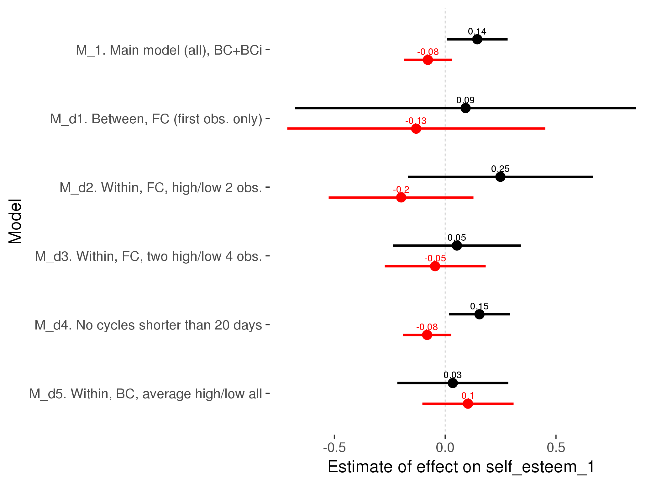
M_m1: Moderation by contraceptive method
Based on the sample with lax exclusion criteria. Users who used any hormonal contraception are classified as hormonal, users who use any awareness-based methods (counting, temperature-based) are classified as ‘fertility-awareness’, women who don’t fall into the before groups and use condoms, pessars, coitus interruptus etc. are classified as ‘barrie or abstinence’. Women who don’t use contraception or use other methods such as sterilisation are excluded from this analysis.
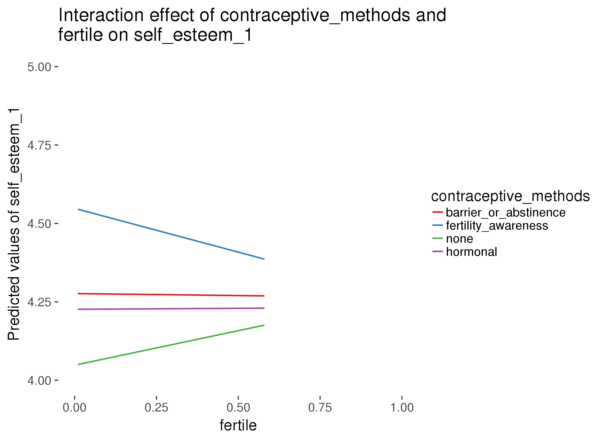
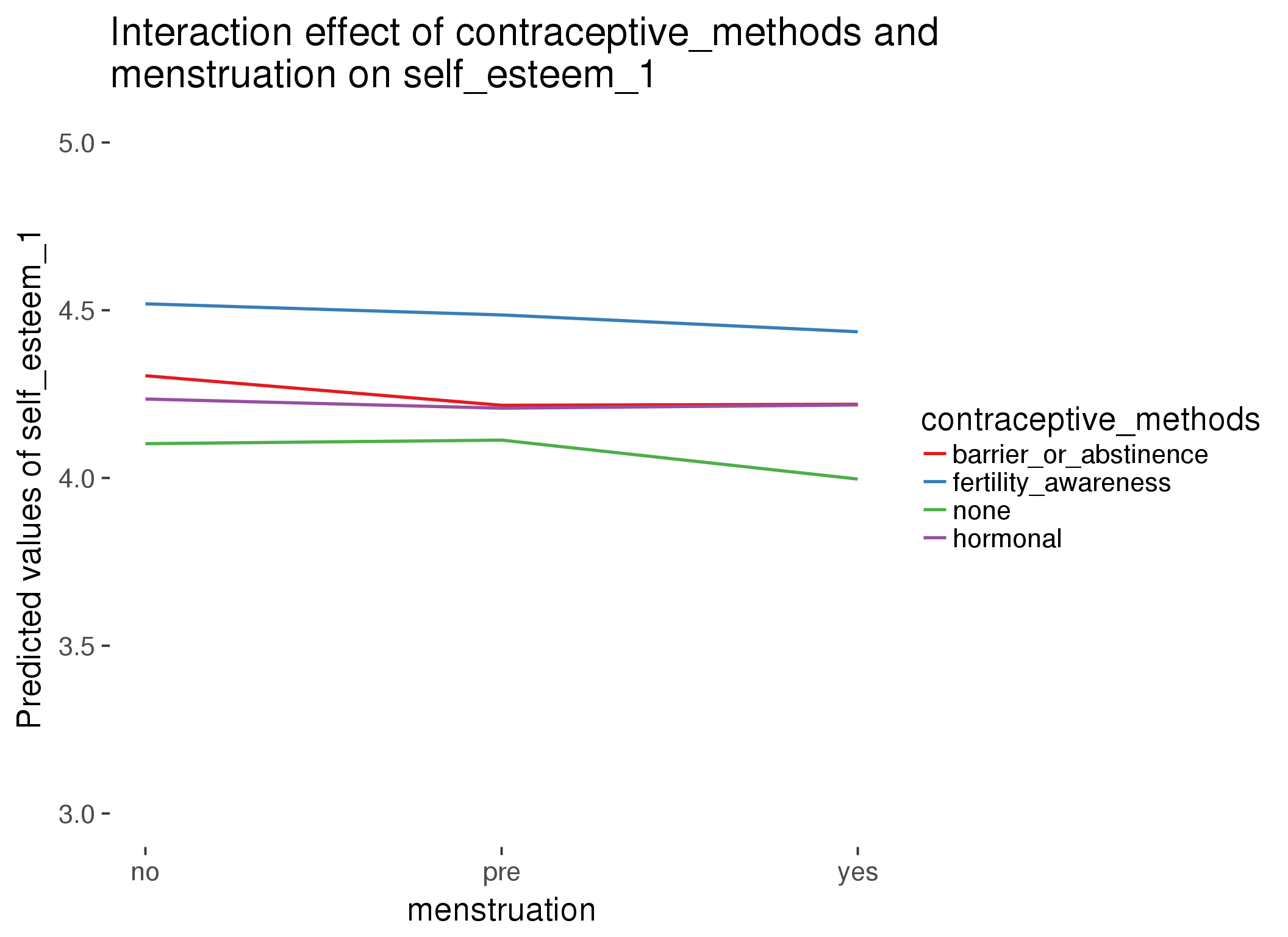
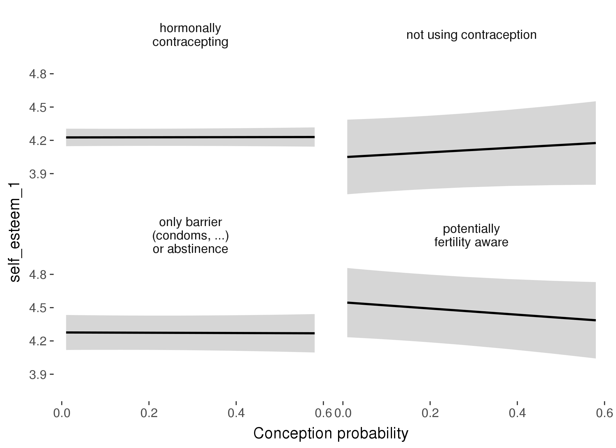
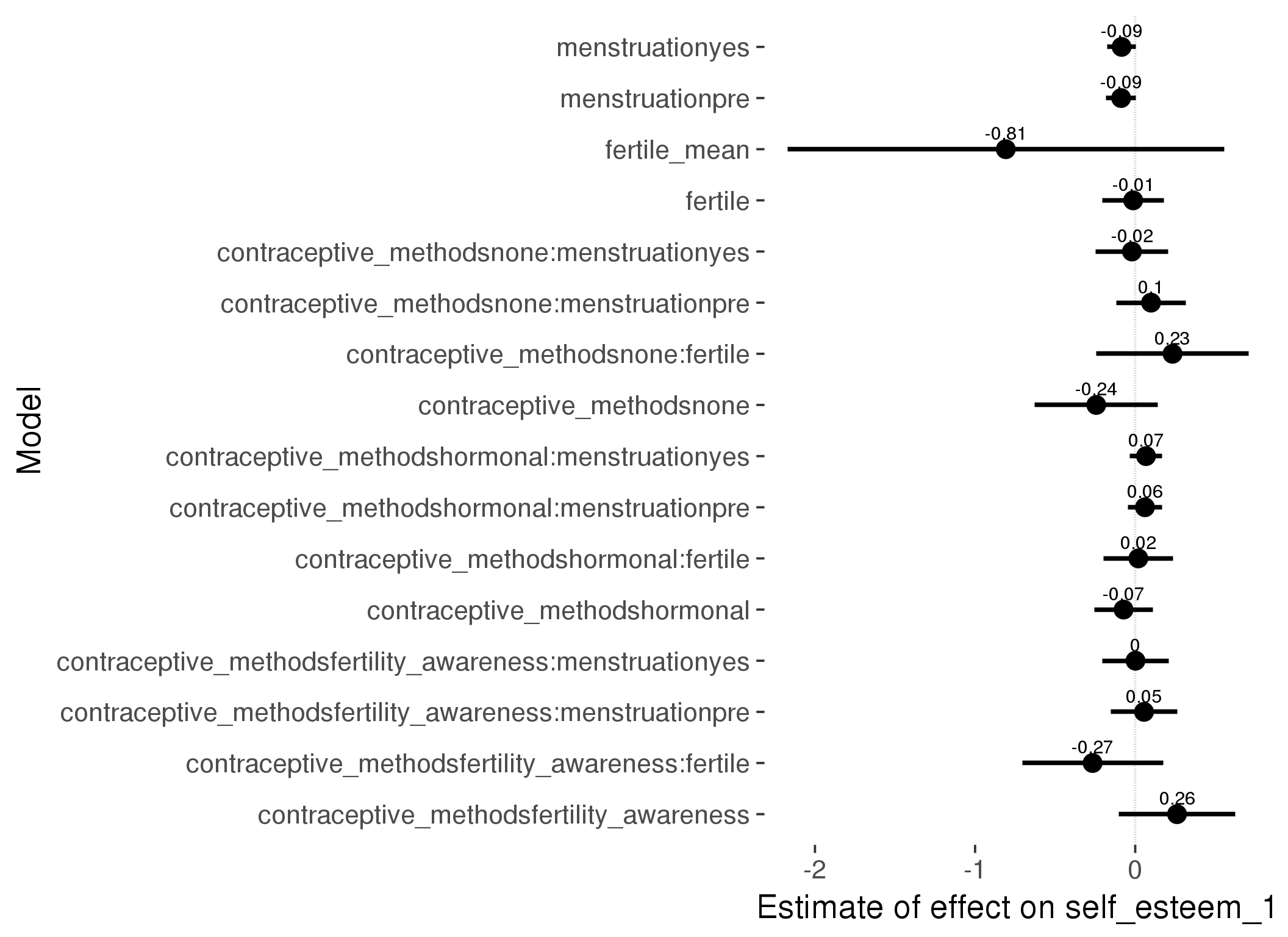
Linear mixed model fit by REML ['lmerMod']
Formula: self_esteem_1 ~ fertile_mean + (1 | person) + contraceptive_methods +
fertile + menstruation + fertile:contraceptive_methods + menstruation:contraceptive_methods
Data: diary
Subset: !is.na(included_lax) & contraceptive_method != "other"
REML criterion at convergence: 45836
Scaled residuals:
Min 1Q Median 3Q Max
-5.276 -0.501 0.097 0.634 3.745
Random effects:
Groups Name Variance Std.Dev.
person (Intercept) 0.557 0.746
Residual 0.783 0.885
Number of obs: 17029, groups: person, 513
Fixed effects:
Estimate Std. Error t value
(Intercept) 4.44870 0.14296 31.12
fertile_mean -0.80827 0.69549 -1.16
contraceptive_methodsfertility_awareness 0.26107 0.18544 1.41
contraceptive_methodsnone -0.24335 0.19654 -1.24
contraceptive_methodshormonal -0.07282 0.09351 -0.78
fertile -0.01294 0.09875 -0.13
menstruationpre -0.08810 0.04769 -1.85
menstruationyes -0.08502 0.04556 -1.87
contraceptive_methodsfertility_awareness:fertile -0.26618 0.22427 -1.19
contraceptive_methodsnone:fertile 0.23302 0.24278 0.96
contraceptive_methodshormonal:fertile 0.01934 0.11032 0.18
contraceptive_methodsfertility_awareness:menstruationpre 0.05496 0.10564 0.52
contraceptive_methodsnone:menstruationpre 0.09870 0.11046 0.89
contraceptive_methodshormonal:menstruationpre 0.06074 0.05372 1.13
contraceptive_methodsfertility_awareness:menstruationyes 0.00171 0.10617 0.02
contraceptive_methodsnone:menstruationyes -0.02049 0.11550 -0.18
contraceptive_methodshormonal:menstruationyes 0.06749 0.05196 1.30
refitting model(s) with ML (instead of REML)
| Df | AIC | BIC | logLik | deviance | Chisq | Chi Df | Pr(>Chisq) | |
|---|---|---|---|---|---|---|---|---|
| add_main | 13 | 45815 | 45915 | -22894 | 45789 | NA | NA | NA |
| by_method | 19 | 45821 | 45968 | -22892 | 45783 | 5.404 | 6 | 0.4931 |
M_m2: Moderation by participant age
model %>%
test_moderator("age_group", diary, xlevels = 5)refitting model(s) with ML (instead of REML)
| Df | AIC | BIC | logLik | deviance | Chisq | Chi Df | Pr(>Chisq) | |
|---|---|---|---|---|---|---|---|---|
| with_main | 19 | 72455 | 72611 | -36209 | 72417 | NA | NA | NA |
| with_mod | 27 | 72456 | 72677 | -36201 | 72402 | 15.36 | 8 | 0.05249 |
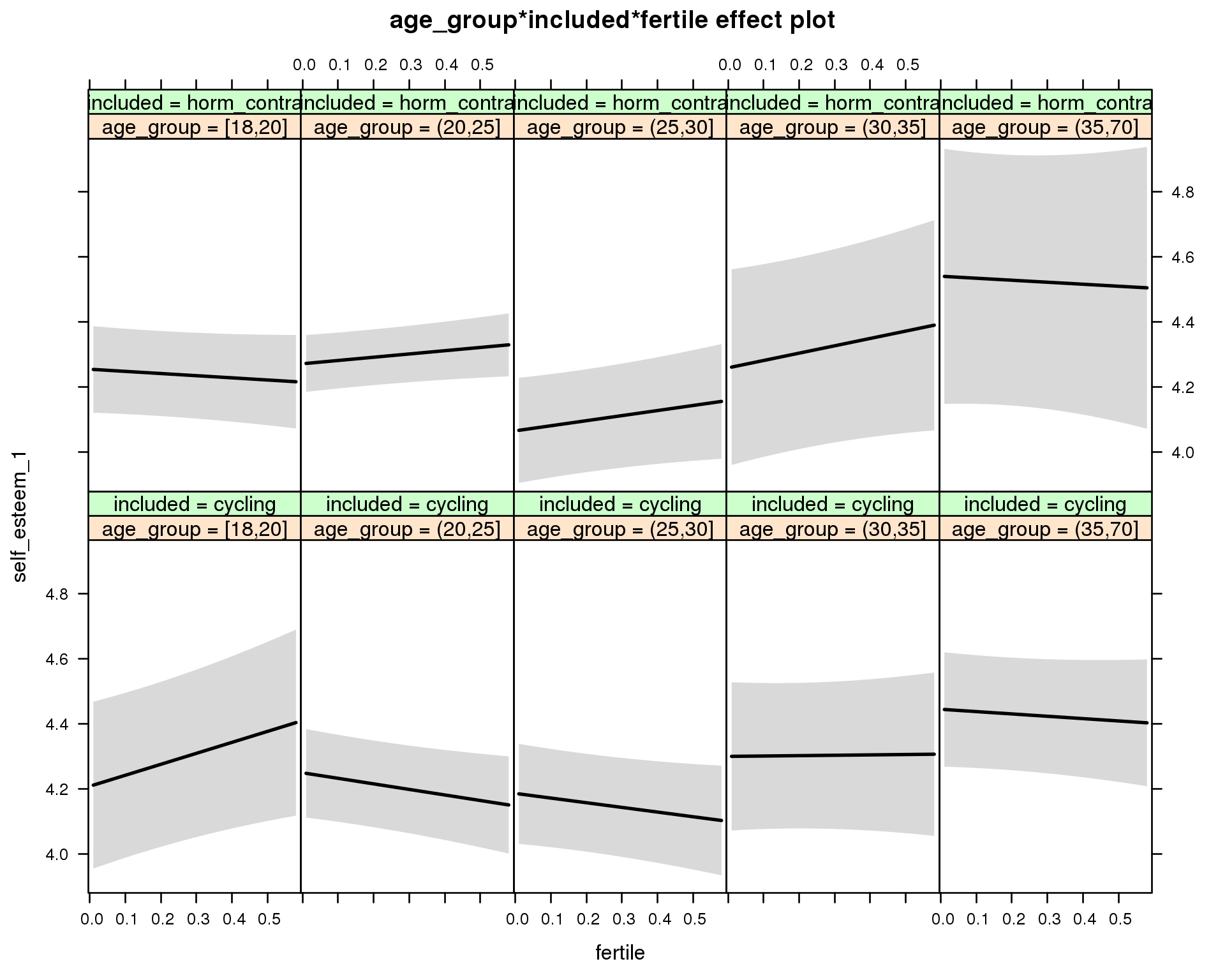
Linear mixed model fit by REML ['lmerMod']
Formula: self_esteem_1 ~ menstruation + fertile_mean + (1 | person) +
age_group + included + fertile + menstruation:included +
age_group:included + age_group:fertile + included:fertile + age_group:included:fertile
Data: diary
REML criterion at convergence: 72480
Scaled residuals:
Min 1Q Median 3Q Max
-5.225 -0.496 0.097 0.630 4.401
Random effects:
Groups Name Variance Std.Dev.
person (Intercept) 0.581 0.762
Residual 0.793 0.890
Number of obs: 26685, groups: person, 1054
Fixed effects:
Estimate Std. Error t value
(Intercept) 4.2655 0.1384 30.82
menstruationpre -0.0514 0.0272 -1.89
menstruationyes -0.1195 0.0256 -4.66
fertile_mean -0.1576 0.3032 -0.52
age_group(20,25] 0.0413 0.1482 0.28
age_group(25,30] -0.0221 0.1526 -0.14
age_group(30,35] 0.0916 0.1751 0.52
age_group(35,70] 0.2364 0.1586 1.49
includedhorm_contra 0.0164 0.1485 0.11
fertile 0.3369 0.1569 2.15
menstruationpre:includedhorm_contra 0.0531 0.0349 1.52
menstruationyes:includedhorm_contra 0.1212 0.0336 3.61
age_group(20,25]:includedhorm_contra -0.0244 0.1691 -0.14
age_group(25,30]:includedhorm_contra -0.1672 0.1862 -0.90
age_group(30,35]:includedhorm_contra -0.0874 0.2425 -0.36
age_group(35,70]:includedhorm_contra 0.0493 0.2644 0.19
age_group(20,25]:fertile -0.5072 0.1738 -2.92
age_group(25,30]:fertile -0.4803 0.1792 -2.68
age_group(30,35]:fertile -0.3254 0.2075 -1.57
age_group(35,70]:fertile -0.4087 0.1872 -2.18
includedhorm_contra:fertile -0.4031 0.1740 -2.32
age_group(20,25]:includedhorm_contra:fertile 0.6735 0.1947 3.46
age_group(25,30]:includedhorm_contra:fertile 0.7023 0.2158 3.25
age_group(30,35]:includedhorm_contra:fertile 0.6176 0.2785 2.22
age_group(35,70]:includedhorm_contra:fertile 0.4135 0.3164 1.31
M_m3: Moderation by weekend
model %>%
test_moderator("weekend", diary, xlevels = 2) refitting model(s) with ML (instead of REML)
| Df | AIC | BIC | logLik | deviance | Chisq | Chi Df | Pr(>Chisq) | |
|---|---|---|---|---|---|---|---|---|
| with_main | 13 | 72394 | 72501 | -36184 | 72368 | NA | NA | NA |
| with_mod | 15 | 72397 | 72519 | -36183 | 72367 | 1.737 | 2 | 0.4197 |
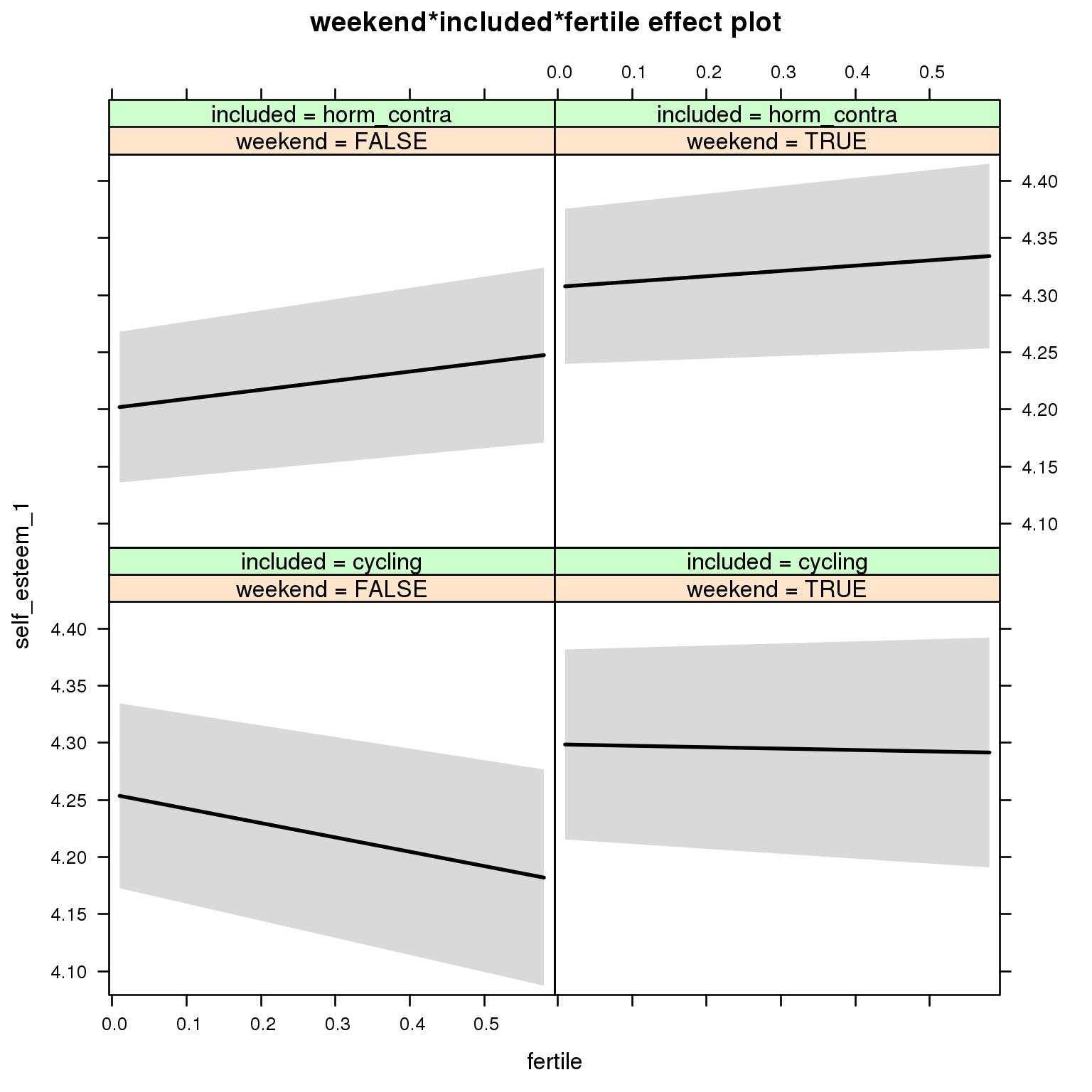
Linear mixed model fit by REML ['lmerMod']
Formula: self_esteem_1 ~ menstruation + fertile_mean + (1 | person) +
weekend + included + fertile + menstruation:included + weekend:included +
weekend:fertile + included:fertile + weekend:included:fertile
Data: diary
REML criterion at convergence: 72428
Scaled residuals:
Min 1Q Median 3Q Max
-5.323 -0.493 0.090 0.634 4.366
Random effects:
Groups Name Variance Std.Dev.
person (Intercept) 0.583 0.764
Residual 0.791 0.890
Number of obs: 26685, groups: person, 1054
Fixed effects:
Estimate Std. Error t value
(Intercept) 4.3204 0.0667 64.8
menstruationpre -0.0528 0.0272 -1.9
menstruationyes -0.1204 0.0256 -4.7
fertile_mean -0.2026 0.3023 -0.7
weekendTRUE 0.0438 0.0237 1.8
includedhorm_contra -0.0847 0.0555 -1.5
fertile -0.1255 0.0667 -1.9
menstruationpre:includedhorm_contra 0.0540 0.0349 1.5
menstruationyes:includedhorm_contra 0.1236 0.0336 3.7
weekendTRUE:includedhorm_contra 0.0622 0.0305 2.0
weekendTRUE:fertile 0.1132 0.0918 1.2
includedhorm_contra:fertile 0.2053 0.0847 2.4
weekendTRUE:includedhorm_contra:fertile -0.1466 0.1167 -1.3
M_m4: Moderation by weekday
model %>%
test_moderator("weekday", diary, xlevels = 7)refitting model(s) with ML (instead of REML)
| Df | AIC | BIC | logLik | deviance | Chisq | Chi Df | Pr(>Chisq) | |
|---|---|---|---|---|---|---|---|---|
| with_main | 23 | 72408 | 72596 | -36181 | 72362 | NA | NA | NA |
| with_mod | 35 | 72419 | 72706 | -36174 | 72349 | 12.87 | 12 | 0.3786 |
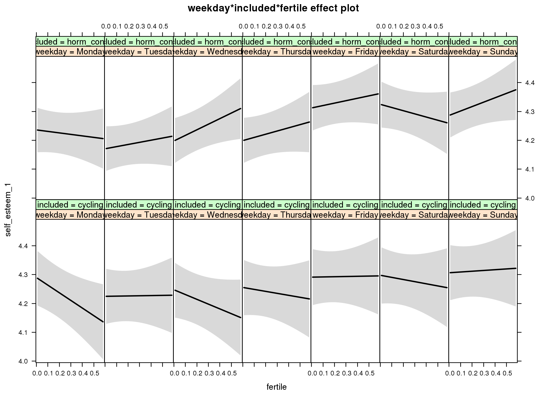
Linear mixed model fit by REML ['lmerMod']
Formula: self_esteem_1 ~ menstruation + fertile_mean + (1 | person) +
weekday + included + fertile + menstruation:included + weekday:included +
weekday:fertile + included:fertile + weekday:included:fertile
Data: diary
REML criterion at convergence: 72486
Scaled residuals:
Min 1Q Median 3Q Max
-5.257 -0.493 0.091 0.632 4.337
Random effects:
Groups Name Variance Std.Dev.
person (Intercept) 0.583 0.764
Residual 0.791 0.890
Number of obs: 26685, groups: person, 1054
Fixed effects:
Estimate Std. Error t value
(Intercept) 4.356578 0.071556 60.9
menstruationpre -0.052599 0.027168 -1.9
menstruationyes -0.120450 0.025600 -4.7
fertile_mean -0.208725 0.302303 -0.7
weekdayTuesday -0.065259 0.042354 -1.5
weekdayWednesday -0.042540 0.042284 -1.0
weekdayThursday -0.034369 0.042766 -0.8
weekdayFriday 0.001214 0.043488 0.0
weekdaySaturday 0.007781 0.043923 0.2
weekdaySunday 0.016403 0.042445 0.4
includedhorm_contra -0.084991 0.064575 -1.3
fertile -0.264502 0.119294 -2.2
menstruationpre:includedhorm_contra 0.053901 0.034876 1.5
menstruationyes:includedhorm_contra 0.123714 0.033561 3.7
weekdayTuesday:includedhorm_contra -0.000121 0.054409 0.0
weekdayWednesday:includedhorm_contra 0.004215 0.054590 0.1
weekdayThursday:includedhorm_contra -0.002812 0.055110 -0.1
weekdayFriday:includedhorm_contra 0.074754 0.055865 1.3
weekdaySaturday:includedhorm_contra 0.080816 0.056518 1.4
weekdaySunday:includedhorm_contra 0.033713 0.054783 0.6
weekdayTuesday:fertile 0.271076 0.164215 1.7
weekdayWednesday:fertile 0.098693 0.164980 0.6
weekdayThursday:fertile 0.195834 0.167341 1.2
weekdayFriday:fertile 0.271893 0.167629 1.6
weekdaySaturday:fertile 0.190525 0.169858 1.1
weekdaySunday:fertile 0.291090 0.165074 1.8
includedhorm_contra:fertile 0.212573 0.152593 1.4
weekdayTuesday:includedhorm_contra:fertile -0.144807 0.209590 -0.7
weekdayWednesday:includedhorm_contra:fertile 0.146791 0.211240 0.7
weekdayThursday:includedhorm_contra:fertile -0.032842 0.212937 -0.2
weekdayFriday:includedhorm_contra:fertile -0.135900 0.213599 -0.6
weekdaySaturday:includedhorm_contra:fertile -0.248804 0.216683 -1.1
weekdaySunday:includedhorm_contra:fertile -0.086130 0.210854 -0.4
M_m5: Moderation by exclusion threshold
model %>%
test_moderator("included_levels", diary, xlevels = 4)refitting model(s) with ML (instead of REML)
| Df | AIC | BIC | logLik | deviance | Chisq | Chi Df | Pr(>Chisq) | |
|---|---|---|---|---|---|---|---|---|
| with_main | 17 | 72457 | 72597 | -36212 | 72423 | NA | NA | NA |
| with_mod | 23 | 72453 | 72642 | -36204 | 72407 | 15.9 | 6 | 0.01428 |
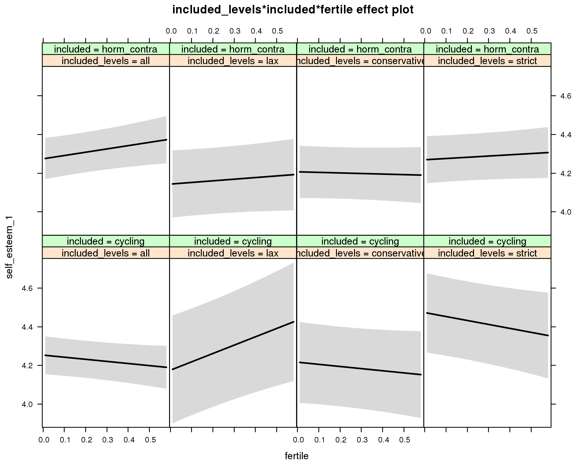
Linear mixed model fit by REML ['lmerMod']
Formula: self_esteem_1 ~ menstruation + fertile_mean + (1 | person) +
included_levels + included + fertile + menstruation:included +
included_levels:included + included_levels:fertile + included:fertile +
included_levels:included:fertile
Data: diary
REML criterion at convergence: 72481
Scaled residuals:
Min 1Q Median 3Q Max
-5.233 -0.492 0.096 0.632 4.377
Random effects:
Groups Name Variance Std.Dev.
person (Intercept) 0.582 0.763
Residual 0.793 0.890
Number of obs: 26685, groups: person, 1054
Fixed effects:
Estimate Std. Error t value
(Intercept) 4.31806 0.07327 58.9
menstruationpre -0.05260 0.02722 -1.9
menstruationyes -0.12150 0.02563 -4.7
fertile_mean -0.19757 0.30476 -0.6
included_levelslax -0.07814 0.15129 -0.5
included_levelsconservative -0.03683 0.11804 -0.3
included_levelsstrict 0.22012 0.11615 1.9
includedhorm_contra -0.00955 0.07565 -0.1
fertile -0.10887 0.06937 -1.6
menstruationpre:includedhorm_contra 0.05304 0.03494 1.5
menstruationyes:includedhorm_contra 0.12079 0.03363 3.6
included_levelslax:includedhorm_contra -0.05269 0.18406 -0.3
included_levelsconservative:includedhorm_contra -0.03050 0.14735 -0.2
included_levelsstrict:includedhorm_contra -0.22502 0.14266 -1.6
included_levelslax:fertile 0.54079 0.16936 3.2
included_levelsconservative:fertile -0.00180 0.12650 0.0
included_levelsstrict:fertile -0.09570 0.12658 -0.8
includedhorm_contra:fertile 0.27925 0.10598 2.6
included_levelslax:includedhorm_contra:fertile -0.62690 0.20665 -3.0
included_levelsconservative:includedhorm_contra:fertile -0.19775 0.16450 -1.2
included_levelsstrict:includedhorm_contra:fertile -0.01068 0.16196 -0.1
M_m6: Moderation by cycle length
model %>%
test_moderator("cycle_length_groups", diary, xlevels = 4)refitting model(s) with ML (instead of REML)
| Df | AIC | BIC | logLik | deviance | Chisq | Chi Df | Pr(>Chisq) | |
|---|---|---|---|---|---|---|---|---|
| with_main | 17 | 72454 | 72594 | -36210 | 72420 | NA | NA | NA |
| with_mod | 23 | 72452 | 72641 | -36203 | 72406 | 14.2 | 6 | 0.02746 |
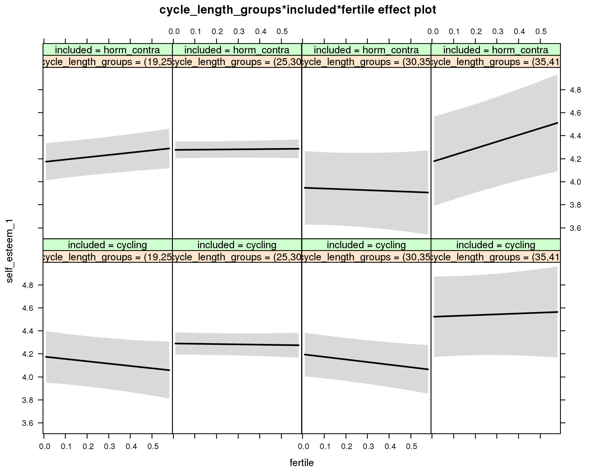
Linear mixed model fit by REML ['lmerMod']
Formula: self_esteem_1 ~ menstruation + fertile_mean + (1 | person) +
cycle_length_groups + included + fertile + menstruation:included +
cycle_length_groups:included + cycle_length_groups:fertile +
included:fertile + cycle_length_groups:included:fertile
Data: diary
REML criterion at convergence: 72472
Scaled residuals:
Min 1Q Median 3Q Max
-5.248 -0.499 0.091 0.632 4.238
Random effects:
Groups Name Variance Std.Dev.
person (Intercept) 0.582 0.763
Residual 0.793 0.890
Number of obs: 26685, groups: person, 1054
Fixed effects:
Estimate Std. Error t value
(Intercept) 4.2459 0.1265 33.6
menstruationpre -0.0511 0.0272 -1.9
menstruationyes -0.1171 0.0258 -4.5
fertile_mean -0.2313 0.3060 -0.8
cycle_length_groups(25,30] 0.1143 0.1244 0.9
cycle_length_groups(30,35] 0.0203 0.1497 0.1
cycle_length_groups(35,41] 0.3458 0.2121 1.6
includedhorm_contra -0.0326 0.1413 -0.2
fertile -0.2028 0.1448 -1.4
menstruationpre:includedhorm_contra 0.0515 0.0349 1.5
menstruationyes:includedhorm_contra 0.1146 0.0338 3.4
cycle_length_groups(25,30]:includedhorm_contra -0.0102 0.1536 -0.1
cycle_length_groups(30,35]:includedhorm_contra -0.2447 0.2359 -1.0
cycle_length_groups(35,41]:includedhorm_contra -0.3452 0.3012 -1.1
cycle_length_groups(25,30]:fertile 0.1762 0.1554 1.1
cycle_length_groups(30,35]:fertile -0.0225 0.1840 -0.1
cycle_length_groups(35,41]:fertile 0.2744 0.2599 1.1
includedhorm_contra:fertile 0.4035 0.1710 2.4
cycle_length_groups(25,30]:includedhorm_contra:fertile -0.3601 0.1841 -2.0
cycle_length_groups(30,35]:includedhorm_contra:fertile -0.2496 0.2897 -0.9
cycle_length_groups(35,41]:includedhorm_contra:fertile 0.1078 0.3421 0.3
M_m7: Moderation by certainty about menstruation parameters
model %>%
test_moderator("certainty_menstruation", diary)refitting model(s) with ML (instead of REML)
| Df | AIC | BIC | logLik | deviance | Chisq | Chi Df | Pr(>Chisq) | |
|---|---|---|---|---|---|---|---|---|
| with_main | 13 | 72446 | 72553 | -36210 | 72420 | NA | NA | NA |
| with_mod | 15 | 72446 | 72569 | -36208 | 72416 | 4.141 | 2 | 0.1261 |
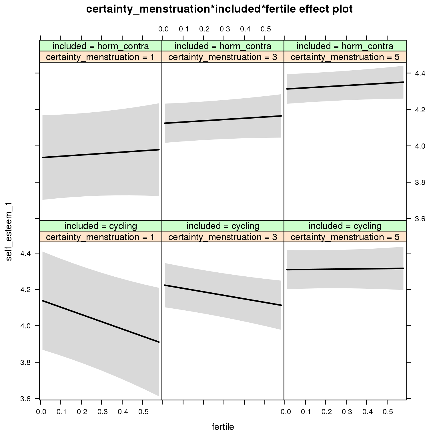
Linear mixed model fit by REML ['lmerMod']
Formula: self_esteem_1 ~ menstruation + fertile_mean + (1 | person) +
certainty_menstruation + included + fertile + menstruation:included +
certainty_menstruation:included + certainty_menstruation:fertile +
included:fertile + certainty_menstruation:included:fertile
Data: diary
REML criterion at convergence: 72476
Scaled residuals:
Min 1Q Median 3Q Max
-5.260 -0.497 0.093 0.632 4.417
Random effects:
Groups Name Variance Std.Dev.
person (Intercept) 0.579 0.761
Residual 0.793 0.891
Number of obs: 26685, groups: person, 1054
Fixed effects:
Estimate Std. Error t value
(Intercept) 4.1742 0.1857 22.47
menstruationpre -0.0508 0.0272 -1.87
menstruationyes -0.1172 0.0257 -4.57
fertile_mean -0.2544 0.3020 -0.84
certainty_menstruation 0.0416 0.0423 0.98
includedhorm_contra -0.2902 0.2358 -1.23
fertile -0.5022 0.2160 -2.33
menstruationpre:includedhorm_contra 0.0530 0.0349 1.52
menstruationyes:includedhorm_contra 0.1191 0.0336 3.54
certainty_menstruation:includedhorm_contra 0.0528 0.0549 0.96
certainty_menstruation:fertile 0.1029 0.0506 2.03
includedhorm_contra:fertile 0.5807 0.2808 2.07
certainty_menstruation:includedhorm_contra:fertile -0.1056 0.0649 -1.63
M_m8: Moderation by cycle regularity
model %>%
test_moderator("cycle_regularity", diary)refitting model(s) with ML (instead of REML)
| Df | AIC | BIC | logLik | deviance | Chisq | Chi Df | Pr(>Chisq) | |
|---|---|---|---|---|---|---|---|---|
| with_main | 15 | 72439 | 72562 | -36205 | 72409 | NA | NA | NA |
| with_mod | 19 | 72433 | 72589 | -36198 | 72395 | 13.79 | 4 | 0.007984 |
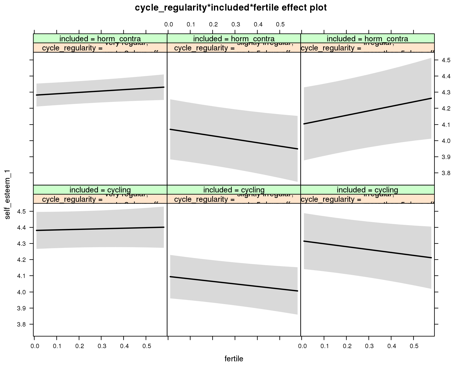
Linear mixed model fit by REML ['lmerMod']
Formula: self_esteem_1 ~ menstruation + fertile_mean + (1 | person) +
cycle_regularity + included + fertile + menstruation:included +
cycle_regularity:included + cycle_regularity:fertile + included:fertile +
cycle_regularity:included:fertile
Data: diary
REML criterion at convergence: 72458
Scaled residuals:
Min 1Q Median 3Q Max
-5.265 -0.498 0.094 0.630 4.405
Random effects:
Groups Name Variance Std.Dev.
person (Intercept) 0.573 0.757
Residual 0.793 0.890
Number of obs: 26685, groups: person, 1054
Fixed effects:
Estimate Std. Error t value
(Intercept) 4.4436 0.0774 57.4
menstruationpre -0.0509 0.0272 -1.9
menstruationyes -0.1188 0.0256 -4.6
fertile_mean -0.1919 0.3018 -0.6
cycle_regularityslightly irregular,\nup to 5 days off -0.2846 0.0901 -3.2
cycle_regularityirregular,\nmore than 5 days off -0.0643 0.1059 -0.6
includedhorm_contra -0.1290 0.0706 -1.8
fertile 0.0346 0.0760 0.5
menstruationpre:includedhorm_contra 0.0519 0.0349 1.5
menstruationyes:includedhorm_contra 0.1194 0.0336 3.6
cycle_regularityslightly irregular,\nup to 5 days off:includedhorm_contra 0.0752 0.1361 0.6
cycle_regularityirregular,\nmore than 5 days off:includedhorm_contra -0.1161 0.1609 -0.7
cycle_regularityslightly irregular,\nup to 5 days off:fertile -0.1898 0.1048 -1.8
cycle_regularityirregular,\nmore than 5 days off:fertile -0.2149 0.1289 -1.7
includedhorm_contra:fertile 0.0509 0.0890 0.6
cycle_regularityslightly irregular,\nup to 5 days off:includedhorm_contra:fertile -0.1080 0.1556 -0.7
cycle_regularityirregular,\nmore than 5 days off:includedhorm_contra:fertile 0.4075 0.1922 2.1
M_m9: Moderation by cohabitation status
model %>%
test_moderator("cohabitation", diary)refitting model(s) with ML (instead of REML)
| Df | AIC | BIC | logLik | deviance | Chisq | Chi Df | Pr(>Chisq) | |
|---|---|---|---|---|---|---|---|---|
| with_main | 15 | 72457 | 72580 | -36214 | 72427 | NA | NA | NA |
| with_mod | 19 | 72445 | 72601 | -36204 | 72407 | 20.25 | 4 | 0.0004456 |
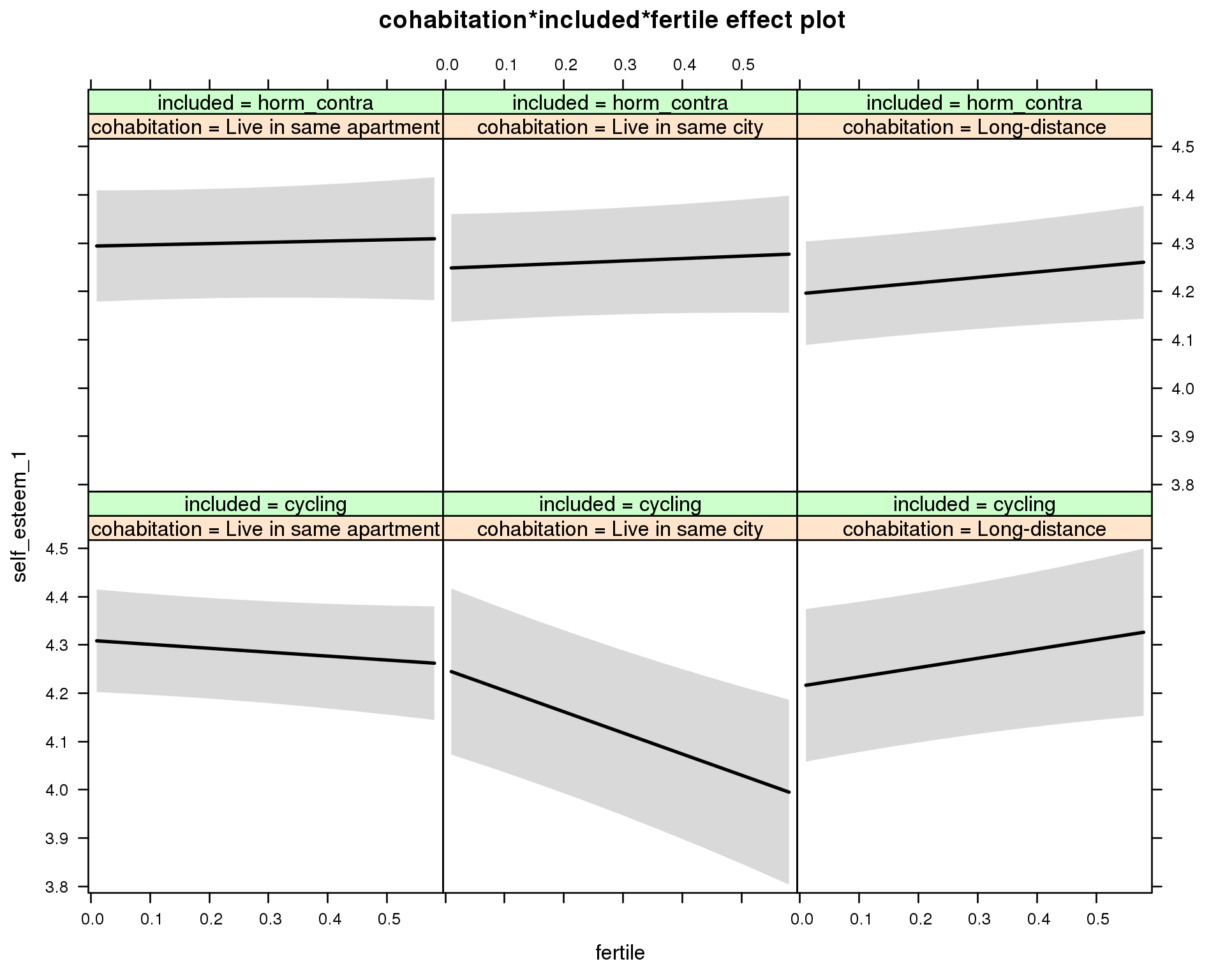
Linear mixed model fit by REML ['lmerMod']
Formula: self_esteem_1 ~ menstruation + fertile_mean + (1 | person) +
cohabitation + included + fertile + menstruation:included +
cohabitation:included + cohabitation:fertile + included:fertile + cohabitation:included:fertile
Data: diary
REML criterion at convergence: 72473
Scaled residuals:
Min 1Q Median 3Q Max
-5.270 -0.497 0.092 0.633 4.421
Random effects:
Groups Name Variance Std.Dev.
person (Intercept) 0.584 0.764
Residual 0.793 0.890
Number of obs: 26685, groups: person, 1054
Fixed effects:
Estimate Std. Error t value
(Intercept) 4.37593 0.07564 57.9
menstruationpre -0.05346 0.02719 -2.0
menstruationyes -0.12211 0.02562 -4.8
fertile_mean -0.20637 0.30313 -0.7
cohabitationLive in same city -0.06017 0.10314 -0.6
cohabitationLong-distance -0.09476 0.09716 -1.0
includedhorm_contra -0.04687 0.08144 -0.6
fertile -0.08124 0.06859 -1.2
menstruationpre:includedhorm_contra 0.05602 0.03490 1.6
menstruationyes:includedhorm_contra 0.12404 0.03359 3.7
cohabitationLive in same city:includedhorm_contra 0.01441 0.13180 0.1
cohabitationLong-distance:includedhorm_contra -0.00384 0.12611 0.0
cohabitationLive in same city:fertile -0.35682 0.12535 -2.8
cohabitationLong-distance:fertile 0.27380 0.11289 2.4
includedhorm_contra:fertile 0.10744 0.10022 1.1
cohabitationLive in same city:includedhorm_contra:fertile 0.38063 0.15671 2.4
cohabitationLong-distance:includedhorm_contra:fertile -0.18760 0.14540 -1.3
M_m10: Moderation by relationship status
model %>%
test_moderator("relationship_status_clean", diary)refitting model(s) with ML (instead of REML)
| Df | AIC | BIC | logLik | deviance | Chisq | Chi Df | Pr(>Chisq) | |
|---|---|---|---|---|---|---|---|---|
| with_main | 15 | 72457 | 72580 | -36213 | 72427 | NA | NA | NA |
| with_mod | 19 | 72461 | 72617 | -36212 | 72423 | 3.735 | 4 | 0.4431 |
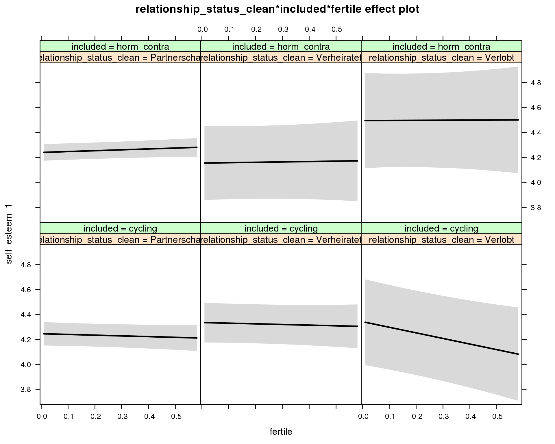
Linear mixed model fit by REML ['lmerMod']
Formula: self_esteem_1 ~ menstruation + fertile_mean + (1 | person) +
relationship_status_clean + included + fertile + menstruation:included +
relationship_status_clean:included + relationship_status_clean:fertile +
included:fertile + relationship_status_clean:included:fertile
Data: diary
REML criterion at convergence: 72480
Scaled residuals:
Min 1Q Median 3Q Max
-5.259 -0.497 0.092 0.632 4.413
Random effects:
Groups Name Variance Std.Dev.
person (Intercept) 0.584 0.764
Residual 0.793 0.891
Number of obs: 26685, groups: person, 1054
Fixed effects:
Estimate Std. Error t value
(Intercept) 4.30982 0.07078 60.9
menstruationpre -0.05308 0.02719 -2.0
menstruationyes -0.12003 0.02563 -4.7
fertile_mean -0.19490 0.30284 -0.6
relationship_status_cleanVerheiratet 0.08966 0.09419 1.0
relationship_status_cleanVerlobt 0.09643 0.18208 0.5
includedhorm_contra -0.03678 0.06072 -0.6
fertile -0.05815 0.06284 -0.9
menstruationpre:includedhorm_contra 0.05490 0.03491 1.6
menstruationyes:includedhorm_contra 0.12154 0.03359 3.6
relationship_status_cleanVerheiratet:includedhorm_contra -0.17490 0.18165 -1.0
relationship_status_cleanVerlobt:includedhorm_contra 0.15916 0.26841 0.6
relationship_status_cleanVerheiratet:fertile 0.00569 0.11064 0.1
relationship_status_cleanVerlobt:fertile -0.38993 0.20750 -1.9
includedhorm_contra:fertile 0.12826 0.07661 1.7
relationship_status_cleanVerheiratet:includedhorm_contra:fertile -0.04481 0.20834 -0.2
relationship_status_cleanVerlobt:includedhorm_contra:fertile 0.32833 0.32224 1.0
Female jealousy
model_summaries$female_jealousyModel summary
Model summary
model %>%
print_summary()Linear mixed model fit by REML
t-tests use Satterthwaite approximations to degrees of freedom ['lmerMod']
Formula: female_jealousy ~ included * (menstruation + fertile) + fertile_mean + (1 | person)
Data: diary
REML criterion at convergence: 54550
Scaled residuals:
Min 1Q Median 3Q Max
-3.613 -0.543 -0.133 0.442 7.291
Random effects:
Groups Name Variance Std.Dev.
person (Intercept) 0.289 0.537
Residual 0.406 0.637
Number of obs: 26682, groups: person, 1054
Fixed effects:
Estimate Std. Error df t value Pr(>|t|)
(Intercept) 1.65631 0.04662 1395.00000 35.53 <2e-16 ***
includedhorm_contra 0.03774 0.03819 1352.00000 0.99 0.32
menstruationpre 0.00781 0.01945 25981.00000 0.40 0.69
menstruationyes 0.01002 0.01832 26086.00000 0.55 0.58
fertile 0.02847 0.03924 25968.00000 0.73 0.47
fertile_mean -0.11271 0.21360 1515.00000 -0.53 0.60
includedhorm_contra:menstruationpre 0.01424 0.02496 25978.00000 0.57 0.57
includedhorm_contra:menstruationyes 0.01087 0.02402 26064.00000 0.45 0.65
includedhorm_contra:fertile -0.00812 0.04972 26089.00000 -0.16 0.87
---
Signif. codes: 0 '***' 0.001 '**' 0.01 '*' 0.05 '.' 0.1 ' ' 1
Correlation of Fixed Effects:
(Intr) incld_ mnstrtnp mnstrtny fertil frtl_m inclddhrm_cntr:mnstrtnp
inclddhrm_c -0.473
menstrutnpr -0.160 0.203
menstrutnys -0.156 0.196 0.397
fertile -0.154 0.252 0.467 0.384
fertile_men -0.772 -0.025 -0.008 -0.005 -0.066
inclddhrm_cntr:mnstrtnp 0.132 -0.255 -0.779 -0.309 -0.363 -0.004
inclddhrm_cntr:mnstrtny 0.125 -0.241 -0.303 -0.763 -0.293 -0.004 0.383
inclddhrm_cntr:f 0.154 -0.318 -0.368 -0.303 -0.787 0.010 0.466
inclddhrm_cntr:mnstrtny
inclddhrm_c
menstrutnpr
menstrutnys
fertile
fertile_men
inclddhrm_cntr:mnstrtnp
inclddhrm_cntr:mnstrtny
inclddhrm_cntr:f 0.381
Effect size standardised by residual variance (\(\frac{b}{ SD_{residual} }\)): 0.04 [-0.08;0.17].
Marginal effect plots
model %>%
plot_all_effects()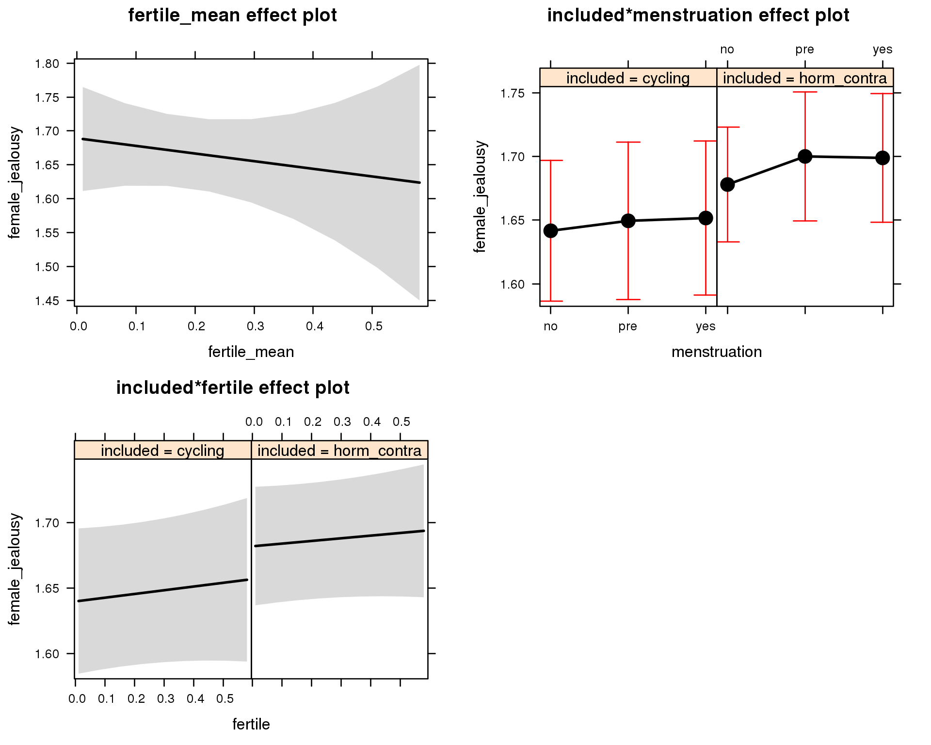
Outcome distribution
model %>%
plot_outcome(diary) + xlab(outcome_label)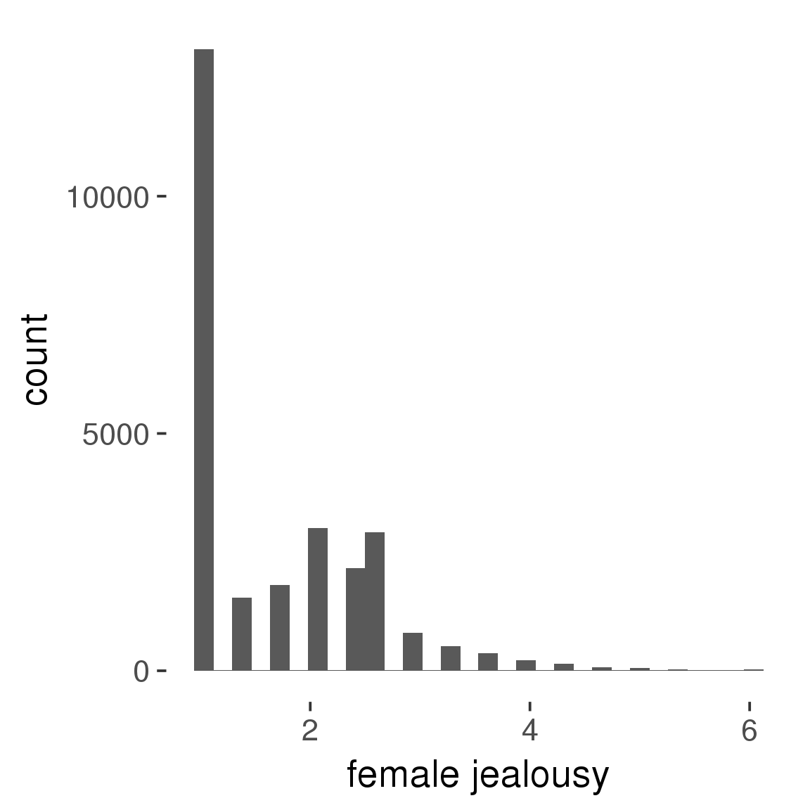
Diagnostics
model %>%
print_diagnostics()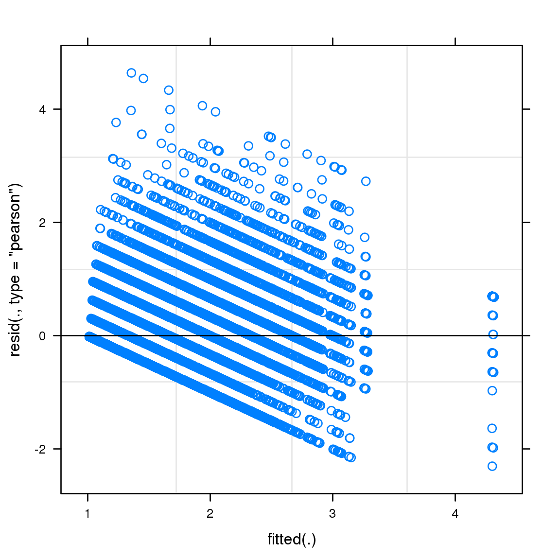
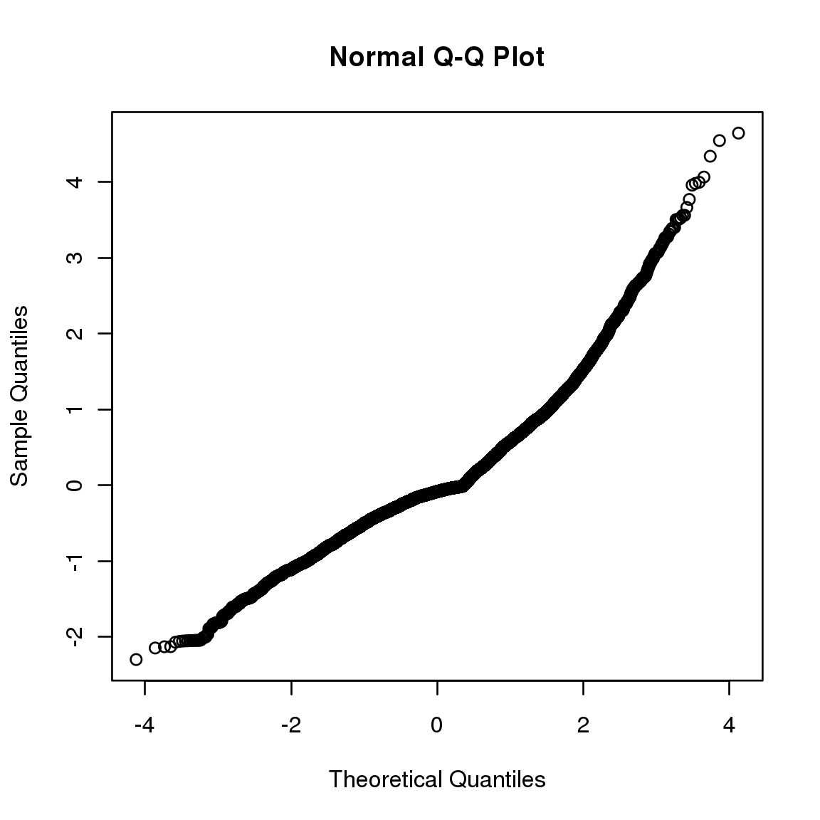

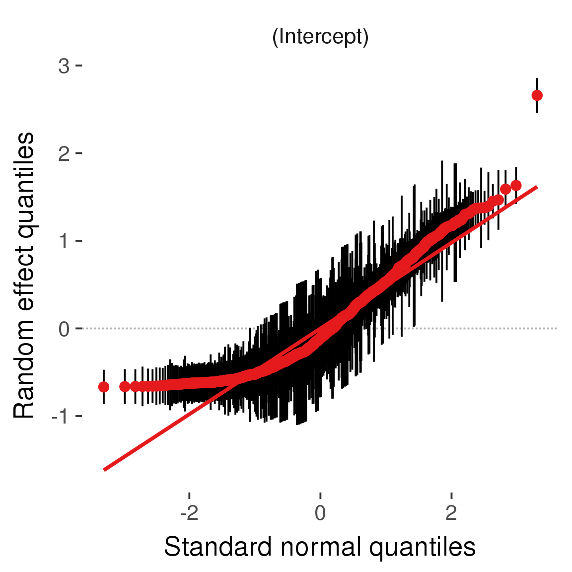
Curves
Here, we continuously plot the outcome over the course of the cycle. Because cycle lengths vary, we subset the data to cycles in a certain range. If the red curve traces the pink curve, our predictor accurately maps the relationship between fertile window probability and the outcome.
Cycle lengths from 21 to 36
Backward-counted
model %>%
plot_curve(diary %>% filter(minimum_cycle_length_diary <= 36, minimum_cycle_length_diary > 20) %>% mutate(fertile=prc_stirn_b))outcome = names(model@frame)[1]
outcome_label = recode(str_replace_all(str_replace_all(str_replace_all(outcome, "_", " "), " pair", "-pair"), " 1", ""),
"desirability 1" = "self-perceived desirability",
"NARQ admiration" = "narcissistic admiration",
"NARQ rivalry" = "narcissistic rivalry",
"extra-pair" = "extra-pair desire & behaviour",
"had sexual intercourse" = "sexual intercourse")
library(ggplot2)
# form a subset and run the model without the hormonal contraception and the fertility predictors
tmp = diary %>%
filter(!is.na(fertile), !is.na(included),
RCD > -1 * minimum_cycle_length_diary, RCD > -40)
new_form = update.formula(formula(model), new = . ~ . - fertile * included)
tmp$residuals = residuals(update(model, new_form, data = tmp , na.action = na.exclude))
tmp = tmp %>%
filter(!is.na(RCD), !is.na(residuals))
rcd_min = min(tmp$RCD)
tmp$real = FALSE
tmp_before = tmp
tmp_before$RCD = tmp_before$RCD + min(tmp$RCD) - 1
tmp_after = tmp
tmp_after$RCD = tmp_after$RCD - min(tmp$RCD) + 1
tmp$real = TRUE
tmp = bind_rows(tmp_before %>% filter(RCD > rcd_min - 11), tmp, tmp_after %>% filter(RCD < 11))GAM smooth on residuals
Here, we partialled out menstruation and individual random effects, then superimposed estimated probability of being in the fertile window scaled to the range of the estimated means. To address the periodicity of the cycle, we prepended and appended ten days of the timeseries to the end and the beginning of the timeseries. We then estimated the GAM and cut off the appended subsets before plotting.
tryCatch({
trend_plot = ggplot(tmp,aes(x = RCD, y = residuals, colour = included)) +
stat_smooth(geom = 'smooth',size = 0.8, fill = "#9ECAE1", method = 'gam', formula = y ~ s(x))
}, error = function(e){cat_message(e, "danger")})
tryCatch({
trend_data = ggplot_build(trend_plot)$data[[1]]
}, error = function(e){cat_message(e, "danger")})
trend_data$RCD = round(trend_data$x)
trend_data = left_join(trend_data, tmp %>% select(real, RCD,fertile) %>% unique(), by = "RCD")
trend_data %>%
filter(real == TRUE) %>%
mutate(superimposed = ( ( (fertile - 0.01)/0.58) * (max(y)-min(y) ) ) + min(y) ) ->
trend_data
ggplot(trend_data) +
geom_ribbon(aes(x = x, ymin = ymin, ymax = ymax, fill = factor(group)), alpha = 0.2) +
geom_line(aes(x = x, y = y, colour = factor(group)), size = 0.8, stat = "identity") +
scale_x_continuous(caption_x) +
geom_line(aes(x = x, y = superimposed), color = "#a83fbf", size = 1, linetype = 'dashed') +
annotate("text",x = mean(trend_data$x), y = max(trend_data$superimposed,na.rm=T) + 0.1, label = 'superimposed fertility peak', color = "#a83fbf") +
scale_y_continuous(outcome_label) +
ggtitle("GAM smooth, residuals") +
scale_color_manual("Contraception status",values = c("2"="black","1"= "red"), labels = c("2"="hormonally\ncontracepting","1"="cycling"), guide = F) +
scale_fill_manual("Contraception status",values = c("2"="black","1"= "red"), labels = c("2"="hormonally\ncontracepting","1"="cycling"), guide = F)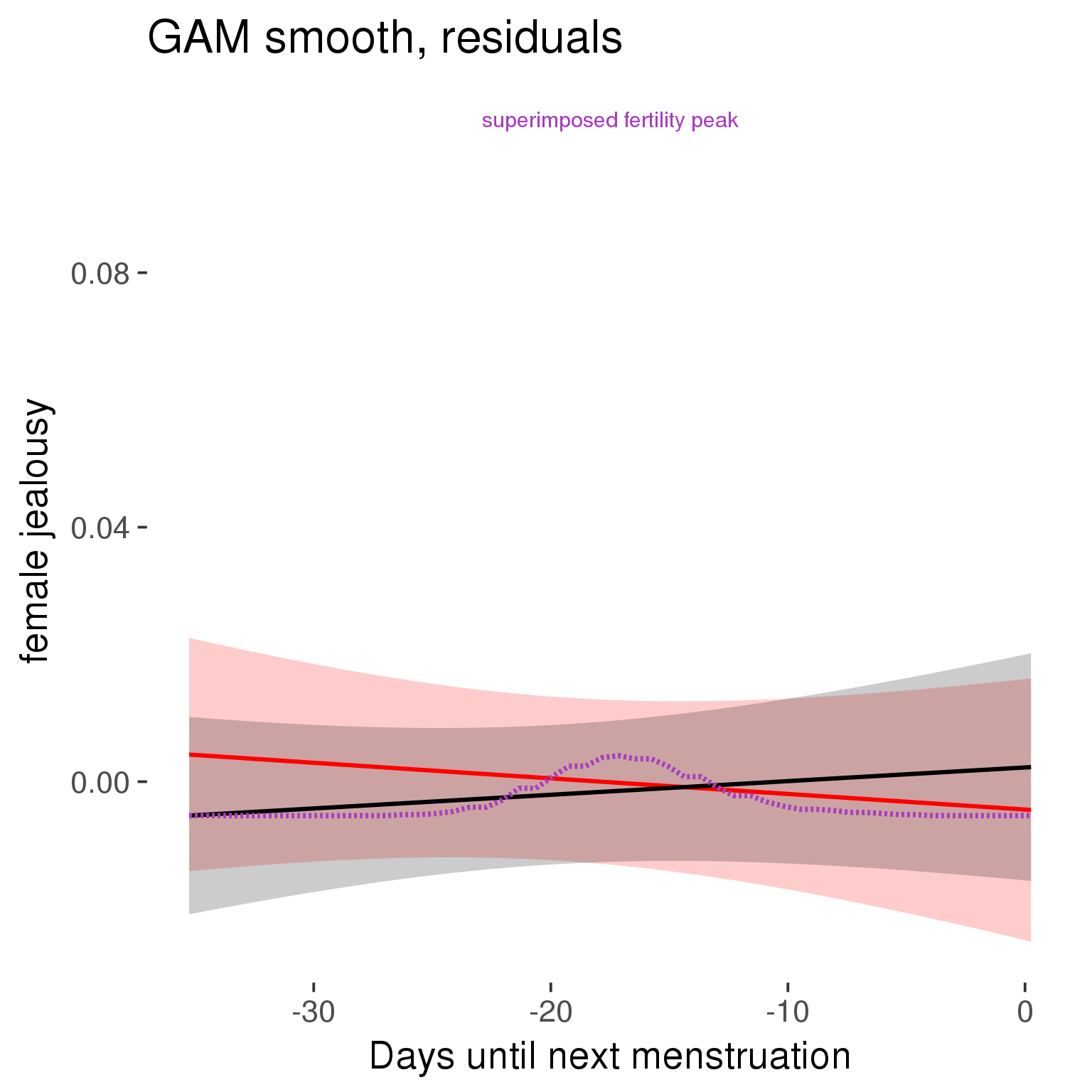
GAM smooth on raw data
As before, but without partialling anything out.
tryCatch({
trend_plot = ggplot(tmp,aes_string(x = "RCD", y = outcome, colour = "included")) +
stat_smooth(geom = 'smooth',size = 0.8, fill = "#9ECAE1", method = 'gam', formula = y ~ s(x))
}, error = function(e){cat_message(e, "danger")})
tryCatch({
trend_data = ggplot_build(trend_plot)$data[[1]]
}, error = function(e){cat_message(e, "danger")})
trend_data$RCD = round(trend_data$x)
trend_data = left_join(trend_data, tmp %>% select(real, RCD,fertile) %>% unique(), by = "RCD")
trend_data %>%
filter(real == TRUE) %>%
mutate(superimposed = ( ( (fertile - 0.01)/0.58) * (max(y)-min(y) ) ) + min(y) ) ->
trend_data
plot1b = ggplot(trend_data) +
geom_ribbon(aes(x = x, ymin = ymin, ymax = ymax, fill = factor(group)), alpha = 0.2) +
geom_line(aes(x = x, y = y, colour = factor(group)), size = 0.8, stat = "identity") +
scale_x_continuous(caption_x) +
geom_line(aes(x = x, y = superimposed), color = "#a83fbf", size = 1, linetype = 'dashed') +
annotate("text",x = mean(trend_data$x), y = max(trend_data$superimposed,na.rm=T) + 0.1, label = 'superimposed fertility peak', color = "#a83fbf") +
scale_y_continuous(outcome_label) +
ggtitle("GAM smooth, raw data") +
scale_color_manual("Contraception status",values = c("2"="black","1"= "red"), labels = c("2"="hormonally\ncontracepting","1"="cycling"), guide = F) +
scale_fill_manual("Contraception status",values = c("2"="black","1"= "red"), labels = c("2"="hormonally\ncontracepting","1"="cycling"), guide = F)
suppressWarnings(print(plot1b))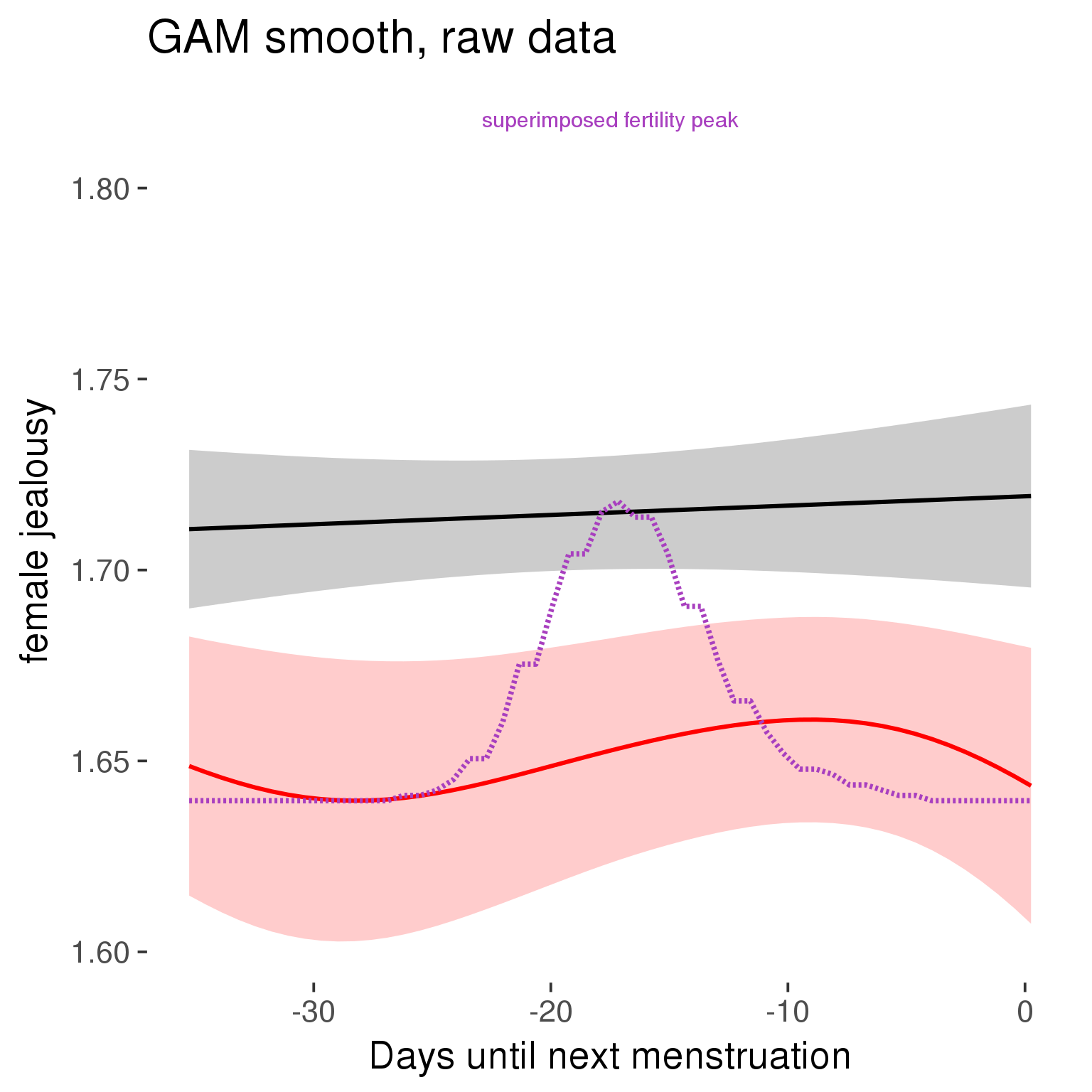
Means and standard errors over raw data
Nothing partialled out, just straight means with bootstrapped confidence intervals.
tryCatch({
trend_plot = ggplot(tmp,aes_string(x = "RCD", y = outcome, colour = "included")) +
geom_pointrange(size = 0.8, stat = 'summary', fun.data = "mean_cl_boot")
}, error = function(e){cat_message(e, "danger")})
tryCatch({
trend_data = ggplot_build(trend_plot)$data[[1]]
}, error = function(e){cat_message(e, "danger")})
trend_data$RCD = round(trend_data$x)
trend_data = left_join(trend_data, tmp %>% select(real, RCD,fertile) %>% unique(), by = "RCD")
trend_data %>%
filter(real == TRUE) %>%
mutate(superimposed = ( ( (fertile - 0.01)/0.58) * (max(y)-min(y) ) ) + min(y) ) ->
trend_data
plot3 = ggplot(trend_data) +
geom_pointrange(aes(x = x, y = y, ymin = ymin,ymax = ymax, colour = factor(group)), size = 0.8, stat = "identity", alpha = 0.6, position = position_dodge(width = .5)) +
scale_x_continuous("Days until next menstruation") +
geom_line(aes(x= x, y = superimposed), color = "#a83fbf", size = 1, linetype = 'dashed') +
annotate("text",x = mean(trend_data$x), y = max(trend_data$superimposed,na.rm=T) + 0.1, label = 'superimposed fertility peak', color = "#a83fbf") +
scale_y_continuous(outcome_label) +
ggtitle("Means with standard errors, raw data") +
scale_color_manual("Contraception status",values = c("2"="black","1"= "red"), labels = c("2"="hormonally\ncontracepting","1"="cycling"), guide = F) +
scale_fill_manual("Contraception status",values = c("2"="black","1"= "red"), labels = c("2"="hormonally\ncontracepting","1"="cycling"), guide = F)
suppressWarnings(print(plot3))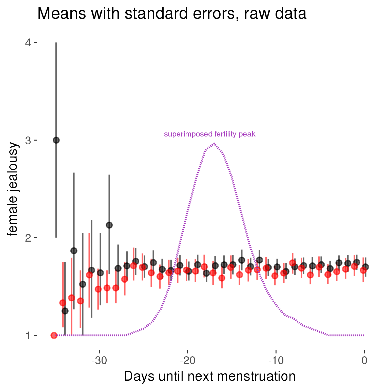
Forward-counted
model %>%
plot_curve(diary %>% filter(minimum_cycle_length_diary <= 36, minimum_cycle_length_diary > 20) %>% mutate(RCD = FCD, fertile = prc_stirn_b_forward_counted), caption_x = "Days since last menstruation")outcome = names(model@frame)[1]
outcome_label = recode(str_replace_all(str_replace_all(str_replace_all(outcome, "_", " "), " pair", "-pair"), " 1", ""),
"desirability 1" = "self-perceived desirability",
"NARQ admiration" = "narcissistic admiration",
"NARQ rivalry" = "narcissistic rivalry",
"extra-pair" = "extra-pair desire & behaviour",
"had sexual intercourse" = "sexual intercourse")
library(ggplot2)
# form a subset and run the model without the hormonal contraception and the fertility predictors
tmp = diary %>%
filter(!is.na(fertile), !is.na(included),
RCD > -1 * minimum_cycle_length_diary, RCD > -40)
new_form = update.formula(formula(model), new = . ~ . - fertile * included)
tmp$residuals = residuals(update(model, new_form, data = tmp , na.action = na.exclude))
tmp = tmp %>%
filter(!is.na(RCD), !is.na(residuals))
rcd_min = min(tmp$RCD)
tmp$real = FALSE
tmp_before = tmp
tmp_before$RCD = tmp_before$RCD + min(tmp$RCD) - 1
tmp_after = tmp
tmp_after$RCD = tmp_after$RCD - min(tmp$RCD) + 1
tmp$real = TRUE
tmp = bind_rows(tmp_before %>% filter(RCD > rcd_min - 11), tmp, tmp_after %>% filter(RCD < 11))GAM smooth on residuals
Here, we partialled out menstruation and individual random effects, then superimposed estimated probability of being in the fertile window scaled to the range of the estimated means. To address the periodicity of the cycle, we prepended and appended ten days of the timeseries to the end and the beginning of the timeseries. We then estimated the GAM and cut off the appended subsets before plotting.
tryCatch({
trend_plot = ggplot(tmp,aes(x = RCD, y = residuals, colour = included)) +
stat_smooth(geom = 'smooth',size = 0.8, fill = "#9ECAE1", method = 'gam', formula = y ~ s(x))
}, error = function(e){cat_message(e, "danger")})
tryCatch({
trend_data = ggplot_build(trend_plot)$data[[1]]
}, error = function(e){cat_message(e, "danger")})
trend_data$RCD = round(trend_data$x)
trend_data = left_join(trend_data, tmp %>% select(real, RCD,fertile) %>% unique(), by = "RCD")
trend_data %>%
filter(real == TRUE) %>%
mutate(superimposed = ( ( (fertile - 0.01)/0.58) * (max(y)-min(y) ) ) + min(y) ) ->
trend_data
ggplot(trend_data) +
geom_ribbon(aes(x = x, ymin = ymin, ymax = ymax, fill = factor(group)), alpha = 0.2) +
geom_line(aes(x = x, y = y, colour = factor(group)), size = 0.8, stat = "identity") +
scale_x_continuous(caption_x) +
geom_line(aes(x = x, y = superimposed), color = "#a83fbf", size = 1, linetype = 'dashed') +
annotate("text",x = mean(trend_data$x), y = max(trend_data$superimposed,na.rm=T) + 0.1, label = 'superimposed fertility peak', color = "#a83fbf") +
scale_y_continuous(outcome_label) +
ggtitle("GAM smooth, residuals") +
scale_color_manual("Contraception status",values = c("2"="black","1"= "red"), labels = c("2"="hormonally\ncontracepting","1"="cycling"), guide = F) +
scale_fill_manual("Contraception status",values = c("2"="black","1"= "red"), labels = c("2"="hormonally\ncontracepting","1"="cycling"), guide = F)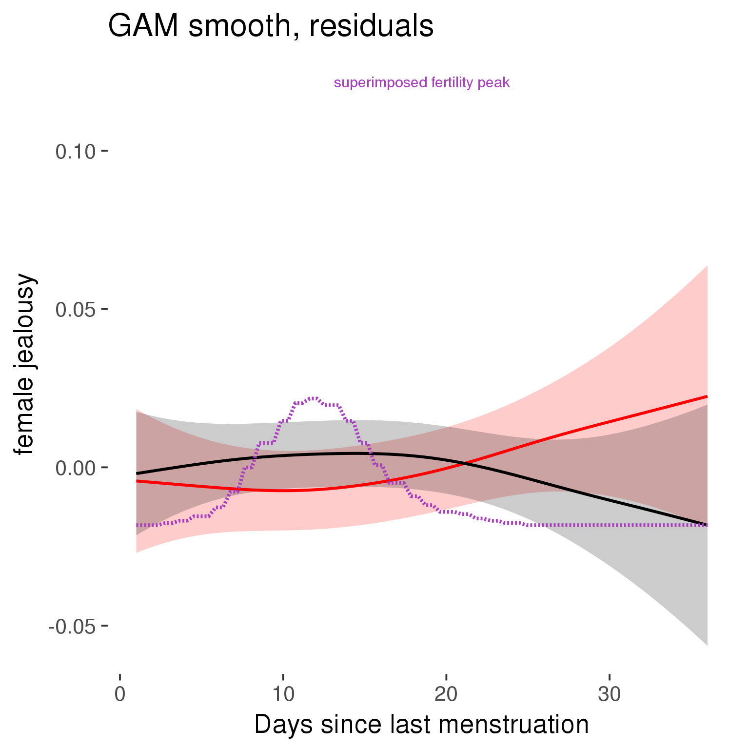
GAM smooth on raw data
As before, but without partialling anything out.
tryCatch({
trend_plot = ggplot(tmp,aes_string(x = "RCD", y = outcome, colour = "included")) +
stat_smooth(geom = 'smooth',size = 0.8, fill = "#9ECAE1", method = 'gam', formula = y ~ s(x))
}, error = function(e){cat_message(e, "danger")})
tryCatch({
trend_data = ggplot_build(trend_plot)$data[[1]]
}, error = function(e){cat_message(e, "danger")})
trend_data$RCD = round(trend_data$x)
trend_data = left_join(trend_data, tmp %>% select(real, RCD,fertile) %>% unique(), by = "RCD")
trend_data %>%
filter(real == TRUE) %>%
mutate(superimposed = ( ( (fertile - 0.01)/0.58) * (max(y)-min(y) ) ) + min(y) ) ->
trend_data
plot1b = ggplot(trend_data) +
geom_ribbon(aes(x = x, ymin = ymin, ymax = ymax, fill = factor(group)), alpha = 0.2) +
geom_line(aes(x = x, y = y, colour = factor(group)), size = 0.8, stat = "identity") +
scale_x_continuous(caption_x) +
geom_line(aes(x = x, y = superimposed), color = "#a83fbf", size = 1, linetype = 'dashed') +
annotate("text",x = mean(trend_data$x), y = max(trend_data$superimposed,na.rm=T) + 0.1, label = 'superimposed fertility peak', color = "#a83fbf") +
scale_y_continuous(outcome_label) +
ggtitle("GAM smooth, raw data") +
scale_color_manual("Contraception status",values = c("2"="black","1"= "red"), labels = c("2"="hormonally\ncontracepting","1"="cycling"), guide = F) +
scale_fill_manual("Contraception status",values = c("2"="black","1"= "red"), labels = c("2"="hormonally\ncontracepting","1"="cycling"), guide = F)
suppressWarnings(print(plot1b))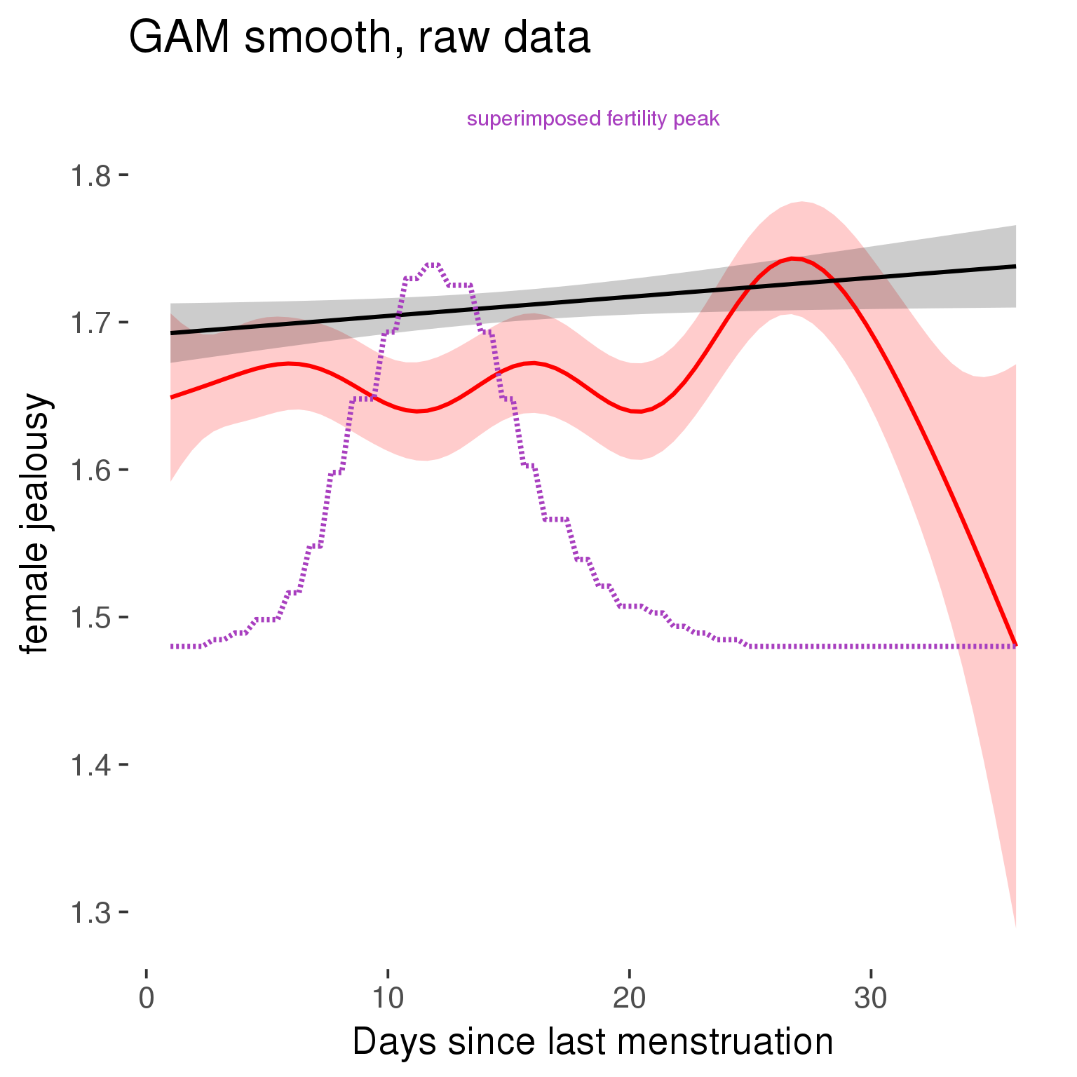
Means and standard errors over raw data
Nothing partialled out, just straight means with bootstrapped confidence intervals.
tryCatch({
trend_plot = ggplot(tmp,aes_string(x = "RCD", y = outcome, colour = "included")) +
geom_pointrange(size = 0.8, stat = 'summary', fun.data = "mean_cl_boot")
}, error = function(e){cat_message(e, "danger")})
tryCatch({
trend_data = ggplot_build(trend_plot)$data[[1]]
}, error = function(e){cat_message(e, "danger")})
trend_data$RCD = round(trend_data$x)
trend_data = left_join(trend_data, tmp %>% select(real, RCD,fertile) %>% unique(), by = "RCD")
trend_data %>%
filter(real == TRUE) %>%
mutate(superimposed = ( ( (fertile - 0.01)/0.58) * (max(y)-min(y) ) ) + min(y) ) ->
trend_data
plot3 = ggplot(trend_data) +
geom_pointrange(aes(x = x, y = y, ymin = ymin,ymax = ymax, colour = factor(group)), size = 0.8, stat = "identity", alpha = 0.6, position = position_dodge(width = .5)) +
scale_x_continuous("Days until next menstruation") +
geom_line(aes(x= x, y = superimposed), color = "#a83fbf", size = 1, linetype = 'dashed') +
annotate("text",x = mean(trend_data$x), y = max(trend_data$superimposed,na.rm=T) + 0.1, label = 'superimposed fertility peak', color = "#a83fbf") +
scale_y_continuous(outcome_label) +
ggtitle("Means with standard errors, raw data") +
scale_color_manual("Contraception status",values = c("2"="black","1"= "red"), labels = c("2"="hormonally\ncontracepting","1"="cycling"), guide = F) +
scale_fill_manual("Contraception status",values = c("2"="black","1"= "red"), labels = c("2"="hormonally\ncontracepting","1"="cycling"), guide = F)
suppressWarnings(print(plot3))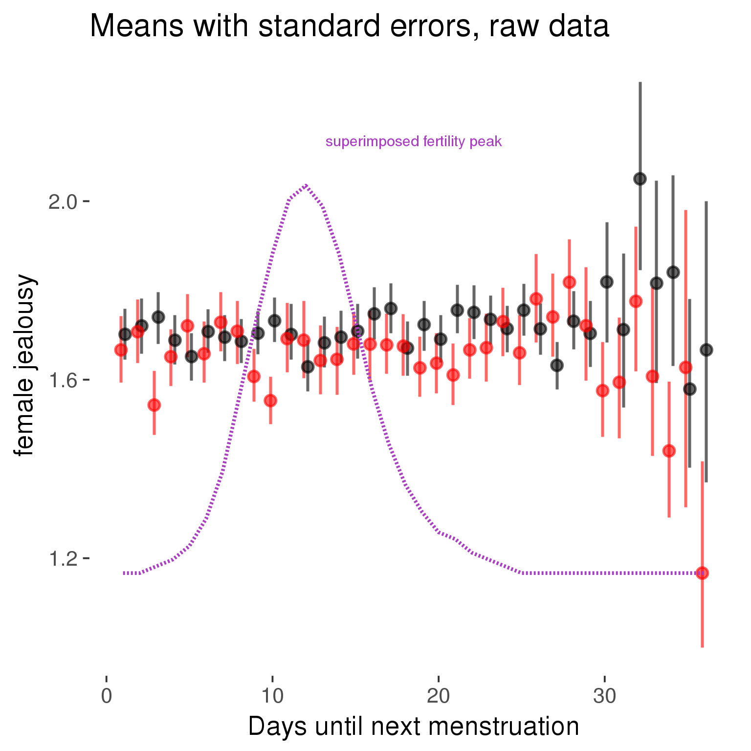
Cycle lengths from 27 to 30
Backward-counted
model %>%
plot_curve(diary %>% filter(minimum_cycle_length_diary <= 30, minimum_cycle_length_diary >= 27) %>% mutate(fertile=prc_stirn_b))outcome = names(model@frame)[1]
outcome_label = recode(str_replace_all(str_replace_all(str_replace_all(outcome, "_", " "), " pair", "-pair"), " 1", ""),
"desirability 1" = "self-perceived desirability",
"NARQ admiration" = "narcissistic admiration",
"NARQ rivalry" = "narcissistic rivalry",
"extra-pair" = "extra-pair desire & behaviour",
"had sexual intercourse" = "sexual intercourse")
library(ggplot2)
# form a subset and run the model without the hormonal contraception and the fertility predictors
tmp = diary %>%
filter(!is.na(fertile), !is.na(included),
RCD > -1 * minimum_cycle_length_diary, RCD > -40)
new_form = update.formula(formula(model), new = . ~ . - fertile * included)
tmp$residuals = residuals(update(model, new_form, data = tmp , na.action = na.exclude))
tmp = tmp %>%
filter(!is.na(RCD), !is.na(residuals))
rcd_min = min(tmp$RCD)
tmp$real = FALSE
tmp_before = tmp
tmp_before$RCD = tmp_before$RCD + min(tmp$RCD) - 1
tmp_after = tmp
tmp_after$RCD = tmp_after$RCD - min(tmp$RCD) + 1
tmp$real = TRUE
tmp = bind_rows(tmp_before %>% filter(RCD > rcd_min - 11), tmp, tmp_after %>% filter(RCD < 11))GAM smooth on residuals
Here, we partialled out menstruation and individual random effects, then superimposed estimated probability of being in the fertile window scaled to the range of the estimated means. To address the periodicity of the cycle, we prepended and appended ten days of the timeseries to the end and the beginning of the timeseries. We then estimated the GAM and cut off the appended subsets before plotting.
tryCatch({
trend_plot = ggplot(tmp,aes(x = RCD, y = residuals, colour = included)) +
stat_smooth(geom = 'smooth',size = 0.8, fill = "#9ECAE1", method = 'gam', formula = y ~ s(x))
}, error = function(e){cat_message(e, "danger")})
tryCatch({
trend_data = ggplot_build(trend_plot)$data[[1]]
}, error = function(e){cat_message(e, "danger")})
trend_data$RCD = round(trend_data$x)
trend_data = left_join(trend_data, tmp %>% select(real, RCD,fertile) %>% unique(), by = "RCD")
trend_data %>%
filter(real == TRUE) %>%
mutate(superimposed = ( ( (fertile - 0.01)/0.58) * (max(y)-min(y) ) ) + min(y) ) ->
trend_data
ggplot(trend_data) +
geom_ribbon(aes(x = x, ymin = ymin, ymax = ymax, fill = factor(group)), alpha = 0.2) +
geom_line(aes(x = x, y = y, colour = factor(group)), size = 0.8, stat = "identity") +
scale_x_continuous(caption_x) +
geom_line(aes(x = x, y = superimposed), color = "#a83fbf", size = 1, linetype = 'dashed') +
annotate("text",x = mean(trend_data$x), y = max(trend_data$superimposed,na.rm=T) + 0.1, label = 'superimposed fertility peak', color = "#a83fbf") +
scale_y_continuous(outcome_label) +
ggtitle("GAM smooth, residuals") +
scale_color_manual("Contraception status",values = c("2"="black","1"= "red"), labels = c("2"="hormonally\ncontracepting","1"="cycling"), guide = F) +
scale_fill_manual("Contraception status",values = c("2"="black","1"= "red"), labels = c("2"="hormonally\ncontracepting","1"="cycling"), guide = F)
GAM smooth on raw data
As before, but without partialling anything out.
tryCatch({
trend_plot = ggplot(tmp,aes_string(x = "RCD", y = outcome, colour = "included")) +
stat_smooth(geom = 'smooth',size = 0.8, fill = "#9ECAE1", method = 'gam', formula = y ~ s(x))
}, error = function(e){cat_message(e, "danger")})
tryCatch({
trend_data = ggplot_build(trend_plot)$data[[1]]
}, error = function(e){cat_message(e, "danger")})
trend_data$RCD = round(trend_data$x)
trend_data = left_join(trend_data, tmp %>% select(real, RCD,fertile) %>% unique(), by = "RCD")
trend_data %>%
filter(real == TRUE) %>%
mutate(superimposed = ( ( (fertile - 0.01)/0.58) * (max(y)-min(y) ) ) + min(y) ) ->
trend_data
plot1b = ggplot(trend_data) +
geom_ribbon(aes(x = x, ymin = ymin, ymax = ymax, fill = factor(group)), alpha = 0.2) +
geom_line(aes(x = x, y = y, colour = factor(group)), size = 0.8, stat = "identity") +
scale_x_continuous(caption_x) +
geom_line(aes(x = x, y = superimposed), color = "#a83fbf", size = 1, linetype = 'dashed') +
annotate("text",x = mean(trend_data$x), y = max(trend_data$superimposed,na.rm=T) + 0.1, label = 'superimposed fertility peak', color = "#a83fbf") +
scale_y_continuous(outcome_label) +
ggtitle("GAM smooth, raw data") +
scale_color_manual("Contraception status",values = c("2"="black","1"= "red"), labels = c("2"="hormonally\ncontracepting","1"="cycling"), guide = F) +
scale_fill_manual("Contraception status",values = c("2"="black","1"= "red"), labels = c("2"="hormonally\ncontracepting","1"="cycling"), guide = F)
suppressWarnings(print(plot1b))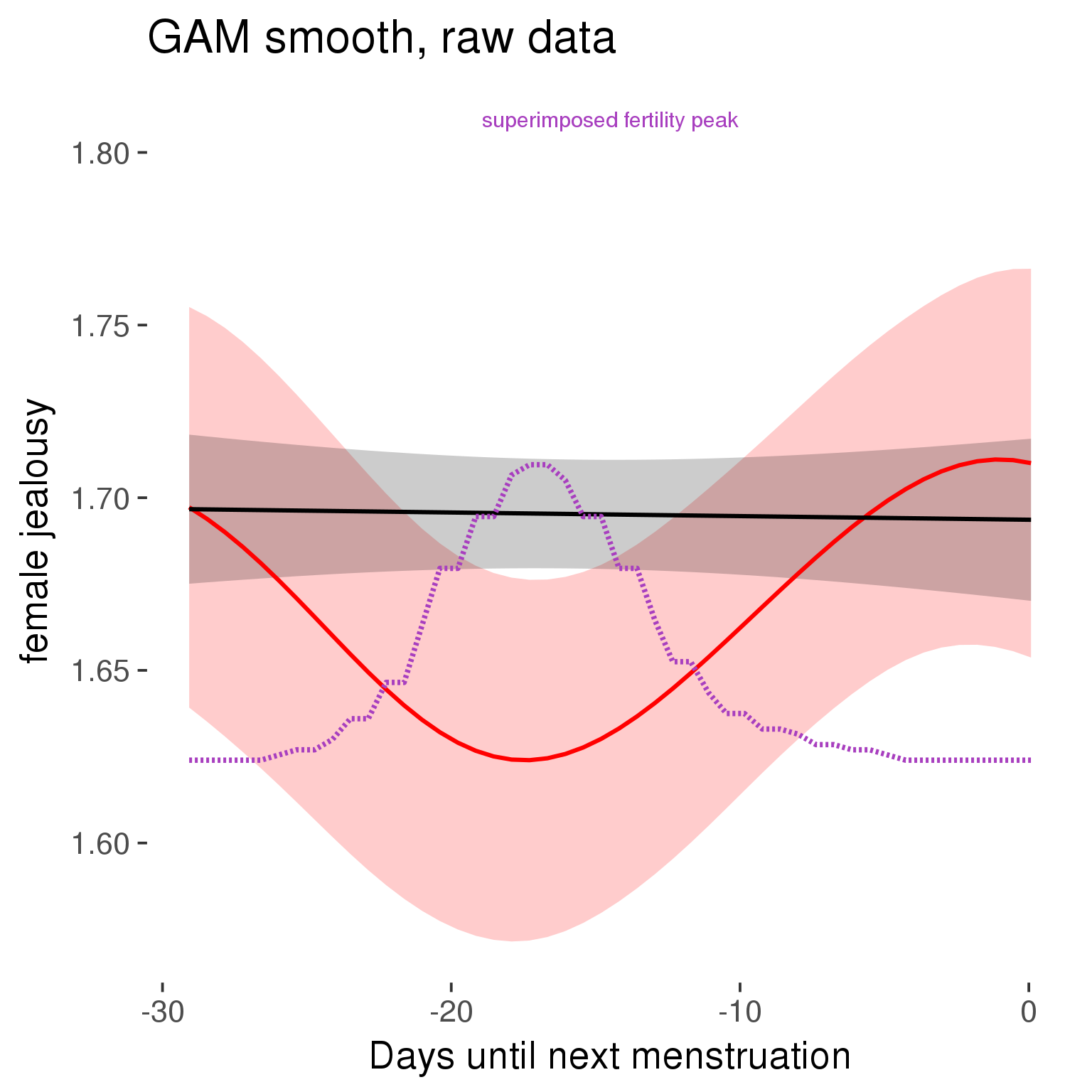
Means and standard errors over raw data
Nothing partialled out, just straight means with bootstrapped confidence intervals.
tryCatch({
trend_plot = ggplot(tmp,aes_string(x = "RCD", y = outcome, colour = "included")) +
geom_pointrange(size = 0.8, stat = 'summary', fun.data = "mean_cl_boot")
}, error = function(e){cat_message(e, "danger")})
tryCatch({
trend_data = ggplot_build(trend_plot)$data[[1]]
}, error = function(e){cat_message(e, "danger")})
trend_data$RCD = round(trend_data$x)
trend_data = left_join(trend_data, tmp %>% select(real, RCD,fertile) %>% unique(), by = "RCD")
trend_data %>%
filter(real == TRUE) %>%
mutate(superimposed = ( ( (fertile - 0.01)/0.58) * (max(y)-min(y) ) ) + min(y) ) ->
trend_data
plot3 = ggplot(trend_data) +
geom_pointrange(aes(x = x, y = y, ymin = ymin,ymax = ymax, colour = factor(group)), size = 0.8, stat = "identity", alpha = 0.6, position = position_dodge(width = .5)) +
scale_x_continuous("Days until next menstruation") +
geom_line(aes(x= x, y = superimposed), color = "#a83fbf", size = 1, linetype = 'dashed') +
annotate("text",x = mean(trend_data$x), y = max(trend_data$superimposed,na.rm=T) + 0.1, label = 'superimposed fertility peak', color = "#a83fbf") +
scale_y_continuous(outcome_label) +
ggtitle("Means with standard errors, raw data") +
scale_color_manual("Contraception status",values = c("2"="black","1"= "red"), labels = c("2"="hormonally\ncontracepting","1"="cycling"), guide = F) +
scale_fill_manual("Contraception status",values = c("2"="black","1"= "red"), labels = c("2"="hormonally\ncontracepting","1"="cycling"), guide = F)
suppressWarnings(print(plot3))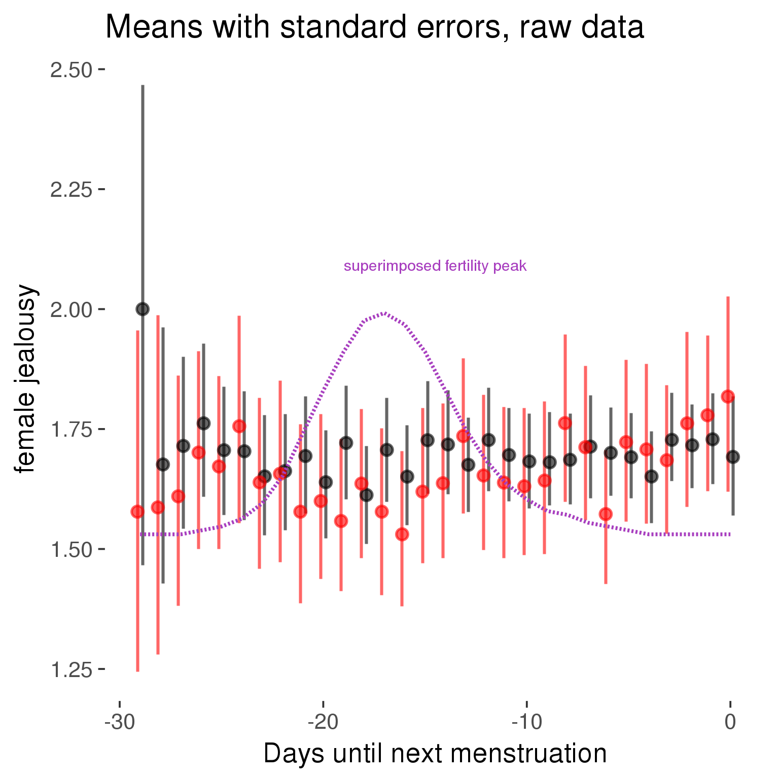
Forward-counted
model %>%
plot_curve(diary %>% filter(minimum_cycle_length_diary <= 30, minimum_cycle_length_diary >= 27) %>% mutate(RCD = FCD, fertile = prc_stirn_b_forward_counted), caption_x = "Days since last menstruation")outcome = names(model@frame)[1]
outcome_label = recode(str_replace_all(str_replace_all(str_replace_all(outcome, "_", " "), " pair", "-pair"), " 1", ""),
"desirability 1" = "self-perceived desirability",
"NARQ admiration" = "narcissistic admiration",
"NARQ rivalry" = "narcissistic rivalry",
"extra-pair" = "extra-pair desire & behaviour",
"had sexual intercourse" = "sexual intercourse")
library(ggplot2)
# form a subset and run the model without the hormonal contraception and the fertility predictors
tmp = diary %>%
filter(!is.na(fertile), !is.na(included),
RCD > -1 * minimum_cycle_length_diary, RCD > -40)
new_form = update.formula(formula(model), new = . ~ . - fertile * included)
tmp$residuals = residuals(update(model, new_form, data = tmp , na.action = na.exclude))
tmp = tmp %>%
filter(!is.na(RCD), !is.na(residuals))
rcd_min = min(tmp$RCD)
tmp$real = FALSE
tmp_before = tmp
tmp_before$RCD = tmp_before$RCD + min(tmp$RCD) - 1
tmp_after = tmp
tmp_after$RCD = tmp_after$RCD - min(tmp$RCD) + 1
tmp$real = TRUE
tmp = bind_rows(tmp_before %>% filter(RCD > rcd_min - 11), tmp, tmp_after %>% filter(RCD < 11))GAM smooth on residuals
Here, we partialled out menstruation and individual random effects, then superimposed estimated probability of being in the fertile window scaled to the range of the estimated means. To address the periodicity of the cycle, we prepended and appended ten days of the timeseries to the end and the beginning of the timeseries. We then estimated the GAM and cut off the appended subsets before plotting.
tryCatch({
trend_plot = ggplot(tmp,aes(x = RCD, y = residuals, colour = included)) +
stat_smooth(geom = 'smooth',size = 0.8, fill = "#9ECAE1", method = 'gam', formula = y ~ s(x))
}, error = function(e){cat_message(e, "danger")})
tryCatch({
trend_data = ggplot_build(trend_plot)$data[[1]]
}, error = function(e){cat_message(e, "danger")})
trend_data$RCD = round(trend_data$x)
trend_data = left_join(trend_data, tmp %>% select(real, RCD,fertile) %>% unique(), by = "RCD")
trend_data %>%
filter(real == TRUE) %>%
mutate(superimposed = ( ( (fertile - 0.01)/0.58) * (max(y)-min(y) ) ) + min(y) ) ->
trend_data
ggplot(trend_data) +
geom_ribbon(aes(x = x, ymin = ymin, ymax = ymax, fill = factor(group)), alpha = 0.2) +
geom_line(aes(x = x, y = y, colour = factor(group)), size = 0.8, stat = "identity") +
scale_x_continuous(caption_x) +
geom_line(aes(x = x, y = superimposed), color = "#a83fbf", size = 1, linetype = 'dashed') +
annotate("text",x = mean(trend_data$x), y = max(trend_data$superimposed,na.rm=T) + 0.1, label = 'superimposed fertility peak', color = "#a83fbf") +
scale_y_continuous(outcome_label) +
ggtitle("GAM smooth, residuals") +
scale_color_manual("Contraception status",values = c("2"="black","1"= "red"), labels = c("2"="hormonally\ncontracepting","1"="cycling"), guide = F) +
scale_fill_manual("Contraception status",values = c("2"="black","1"= "red"), labels = c("2"="hormonally\ncontracepting","1"="cycling"), guide = F)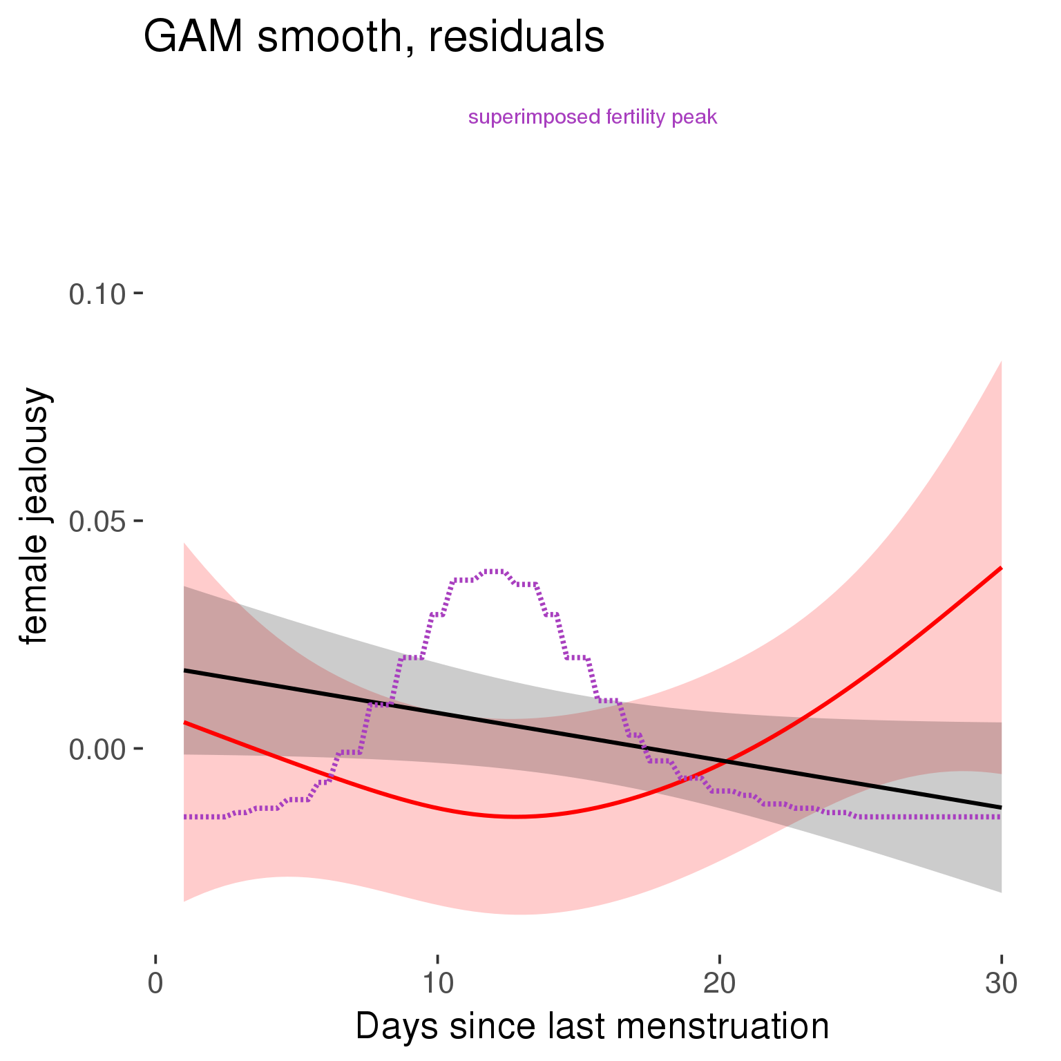
GAM smooth on raw data
As before, but without partialling anything out.
tryCatch({
trend_plot = ggplot(tmp,aes_string(x = "RCD", y = outcome, colour = "included")) +
stat_smooth(geom = 'smooth',size = 0.8, fill = "#9ECAE1", method = 'gam', formula = y ~ s(x))
}, error = function(e){cat_message(e, "danger")})
tryCatch({
trend_data = ggplot_build(trend_plot)$data[[1]]
}, error = function(e){cat_message(e, "danger")})
trend_data$RCD = round(trend_data$x)
trend_data = left_join(trend_data, tmp %>% select(real, RCD,fertile) %>% unique(), by = "RCD")
trend_data %>%
filter(real == TRUE) %>%
mutate(superimposed = ( ( (fertile - 0.01)/0.58) * (max(y)-min(y) ) ) + min(y) ) ->
trend_data
plot1b = ggplot(trend_data) +
geom_ribbon(aes(x = x, ymin = ymin, ymax = ymax, fill = factor(group)), alpha = 0.2) +
geom_line(aes(x = x, y = y, colour = factor(group)), size = 0.8, stat = "identity") +
scale_x_continuous(caption_x) +
geom_line(aes(x = x, y = superimposed), color = "#a83fbf", size = 1, linetype = 'dashed') +
annotate("text",x = mean(trend_data$x), y = max(trend_data$superimposed,na.rm=T) + 0.1, label = 'superimposed fertility peak', color = "#a83fbf") +
scale_y_continuous(outcome_label) +
ggtitle("GAM smooth, raw data") +
scale_color_manual("Contraception status",values = c("2"="black","1"= "red"), labels = c("2"="hormonally\ncontracepting","1"="cycling"), guide = F) +
scale_fill_manual("Contraception status",values = c("2"="black","1"= "red"), labels = c("2"="hormonally\ncontracepting","1"="cycling"), guide = F)
suppressWarnings(print(plot1b))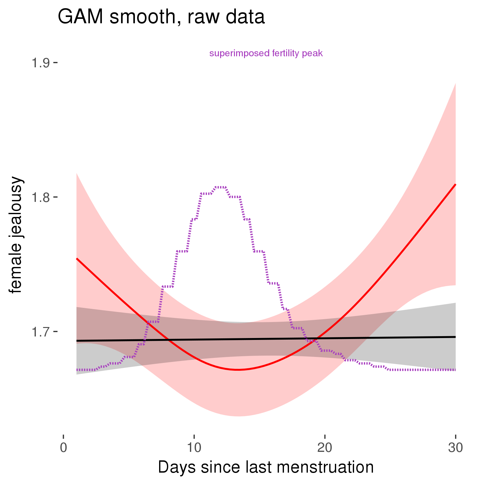
Means and standard errors over raw data
Nothing partialled out, just straight means with bootstrapped confidence intervals.
tryCatch({
trend_plot = ggplot(tmp,aes_string(x = "RCD", y = outcome, colour = "included")) +
geom_pointrange(size = 0.8, stat = 'summary', fun.data = "mean_cl_boot")
}, error = function(e){cat_message(e, "danger")})
tryCatch({
trend_data = ggplot_build(trend_plot)$data[[1]]
}, error = function(e){cat_message(e, "danger")})
trend_data$RCD = round(trend_data$x)
trend_data = left_join(trend_data, tmp %>% select(real, RCD,fertile) %>% unique(), by = "RCD")
trend_data %>%
filter(real == TRUE) %>%
mutate(superimposed = ( ( (fertile - 0.01)/0.58) * (max(y)-min(y) ) ) + min(y) ) ->
trend_data
plot3 = ggplot(trend_data) +
geom_pointrange(aes(x = x, y = y, ymin = ymin,ymax = ymax, colour = factor(group)), size = 0.8, stat = "identity", alpha = 0.6, position = position_dodge(width = .5)) +
scale_x_continuous("Days until next menstruation") +
geom_line(aes(x= x, y = superimposed), color = "#a83fbf", size = 1, linetype = 'dashed') +
annotate("text",x = mean(trend_data$x), y = max(trend_data$superimposed,na.rm=T) + 0.1, label = 'superimposed fertility peak', color = "#a83fbf") +
scale_y_continuous(outcome_label) +
ggtitle("Means with standard errors, raw data") +
scale_color_manual("Contraception status",values = c("2"="black","1"= "red"), labels = c("2"="hormonally\ncontracepting","1"="cycling"), guide = F) +
scale_fill_manual("Contraception status",values = c("2"="black","1"= "red"), labels = c("2"="hormonally\ncontracepting","1"="cycling"), guide = F)
suppressWarnings(print(plot3))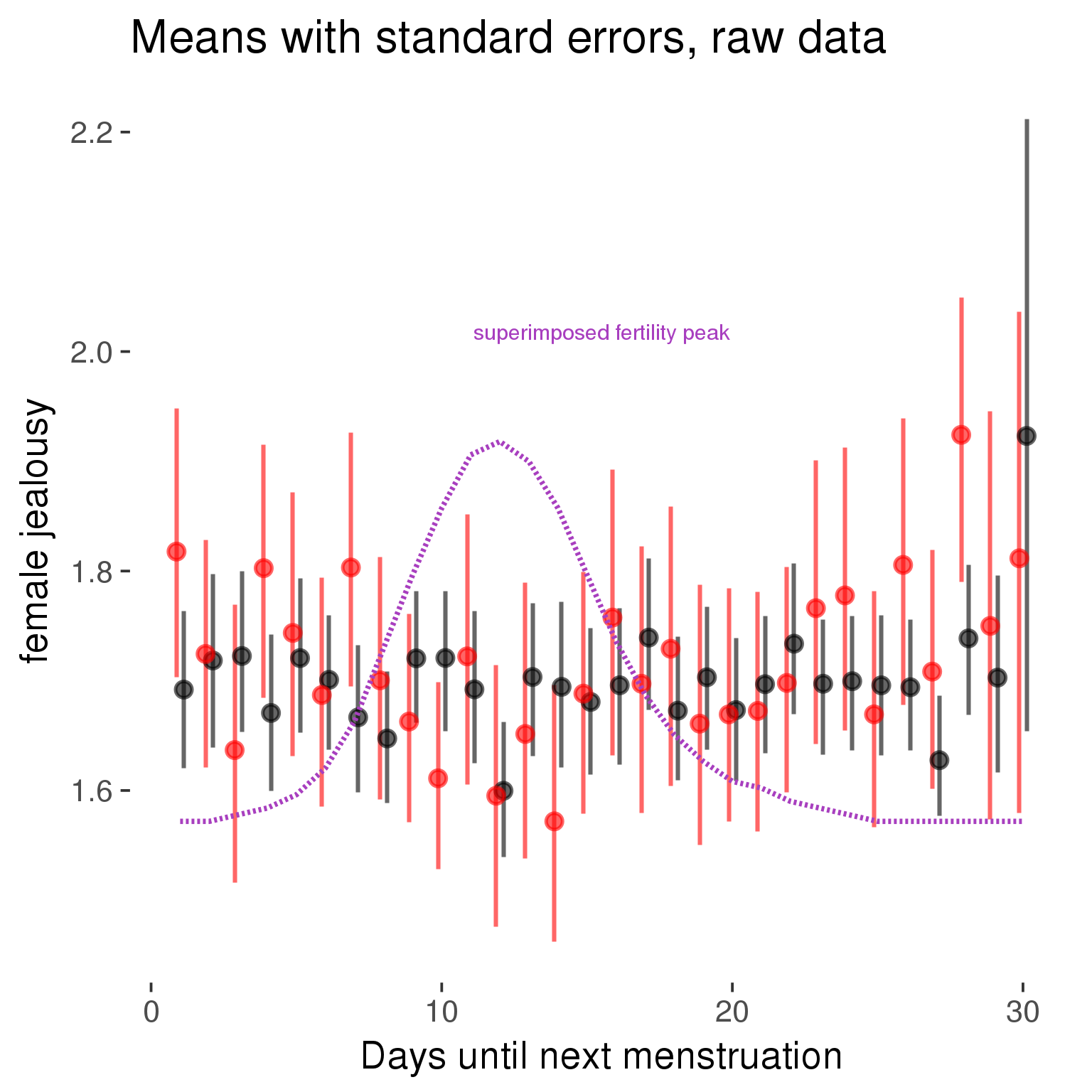
Robustness checks
M_r1: Random slopes for conception risk and menstruation
tryCatch({
# refit model with random effects for fertile and menstruation dummies
with_ind_diff = update(model, formula = . ~ . - (1| person) + (1 + fertile + menstruation | person))
# pull the random effects, format as tibble
rand = coef(with_ind_diff)$person %>%
tibble::rownames_to_column("person") %>%
mutate(person = as.numeric(person))
# pull the fixed effects
fixd = data.frame(fixef(with_ind_diff)) %>%
tibble::rownames_to_column("effect")
names(fixd) = c("effect", "pop_effect_size")
# pull apart the coefficients so that we can account for the fact that the random effect variation implicitly includes HC explaining the mean population-level effect of fertile/menstruation dummies among HC users
fixd = fixd %>%
separate(effect, c("included", "effect"), sep = ":", fill = "left") %>%
mutate(included = if_else(is.na(included), "cycling", str_replace(included, "included", "")))
fixd[2,c("included", "effect")] = c("horm_contra", "(Intercept)")
rand = rand %>%
# merge diary data on the random effects, so that we know who is a HC users and who isn't
inner_join(diary %>% select(person, included) %>% unique(), by = 'person') %>%
# gather into long format, to have the dataset by predictor
gather(effect, value, -person, -included) %>%
inner_join(fixd, by = c('effect', 'included')) %>%
# pull the fixed effects
mutate(
# only for those who are HC users, add the moderated population effect size for this effect (the random effects have the reference category mean)
value = if_else(included == "horm_contra", value + pop_effect_size, value),
effect = recode(effect, "includedhorm_contra" = "HC user",
"includedhorm_contra:fertile" = "HC user x fertile",
"includedhorm_contra:menstruationpre" = "HC user x premens.",
"includedhorm_contra:menstruationyes" = "HC user x mens.",
"menstruationyes" = "mens.",
"menstruationpre" = "premens.")) %>%
group_by(included, effect) %>%
# filter out predictors that aren't modelled as varying/random
filter(sd(value) > 0)
# plot dot plot of random effects
print(
ggplot(rand, aes(x = included, y = value, color = included, fill = included)) +
facet_wrap( ~ effect, scales = "free") +
# geom_violin(alpha = 0.4, size = 0) +
geom_dotplot(binaxis='y', dotsize = 0.1, method = "histodot") +
# geom_jitter(alpha = 0.05) +
coord_flip() +
geom_pointrange(stat = 'summary', fun.data = 'mean_sdl', color = 'darkred', size = 1.2) +
scale_color_manual("Contraception status", values = c("horm_contra"="black","cycling"= "red"), labels = c("horm_contra"="hormonally\ncontracepting","cycling"="cycling"), guide = F) +
scale_fill_manual("Contraception status", values = c("horm_contra"="black","cycling"= "red"), labels = c("horm_contra"="hormonally\ncontracepting","1"="cycling"), guide = F) +
ggtitle("M_r1: allowing participant-varying slopes", subtitle = "for the conception risk measure and the menstruation dummies") +
scale_x_discrete("Hormonal contraception", breaks = c("horm_contra", "cycling"), labels = c("yes", "no")) +
scale_y_continuous("Random effect size distribution"))
print_summary(with_ind_diff)
cat(pander(anova(model, with_ind_diff)))
}, error = function(e){
with_ind_diff = model
cat_message(e, "danger")
})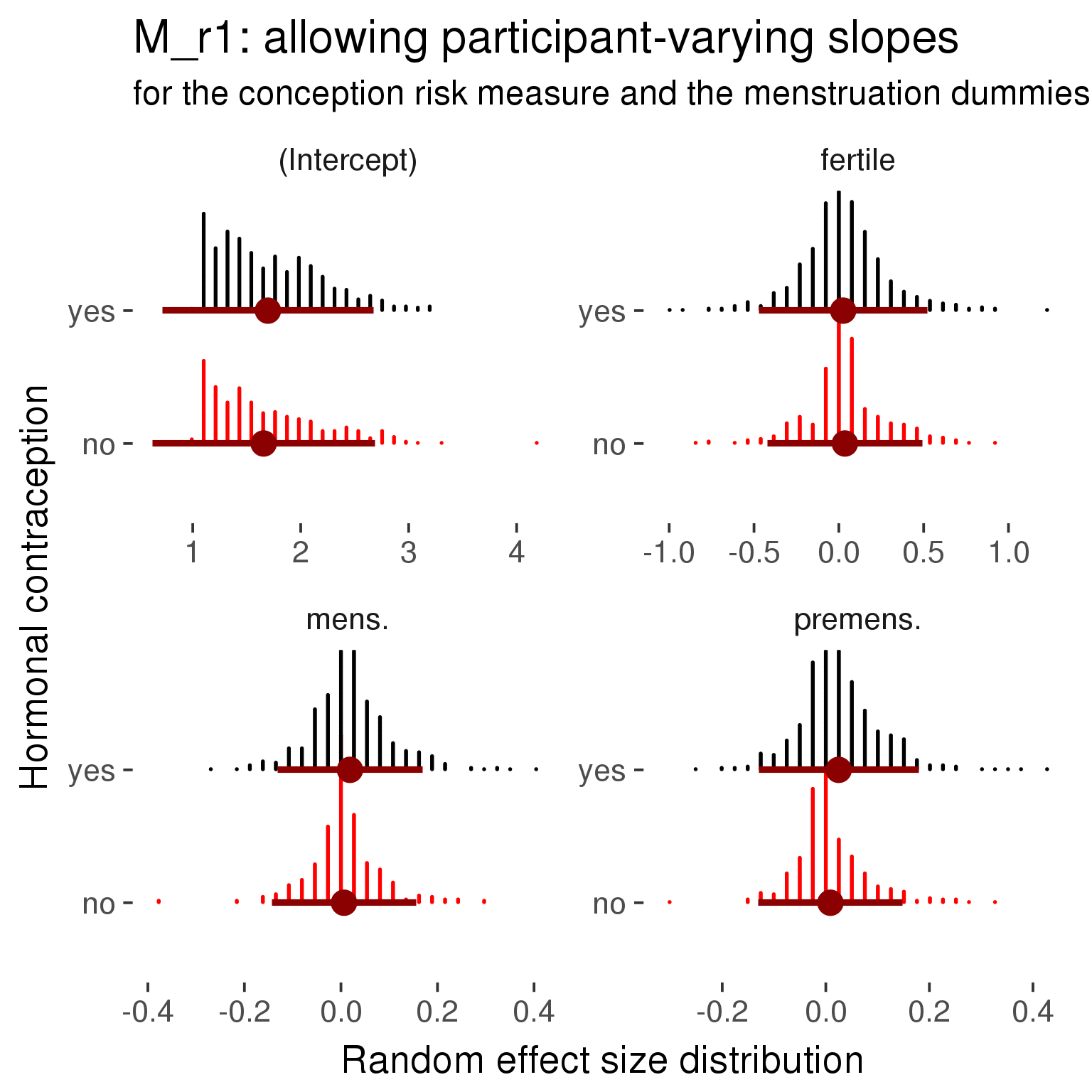
Linear mixed model fit by REML ['lmerMod']
Formula: female_jealousy ~ included + menstruation + fertile + fertile_mean +
(1 + fertile + menstruation | person) + included:menstruation + included:fertile
Data: diary
REML criterion at convergence: 54386
Scaled residuals:
Min 1Q Median 3Q Max
-3.612 -0.533 -0.127 0.441 7.308
Random effects:
Groups Name Variance Std.Dev. Corr
person (Intercept) 0.2885 0.537
fertile 0.2193 0.468 -0.12
menstruationpre 0.0311 0.176 0.07 0.21
menstruationyes 0.0324 0.180 -0.08 0.21 0.25
Residual 0.3910 0.625
Number of obs: 26682, groups: person, 1054
Fixed effects:
Estimate Std. Error t value
(Intercept) 1.65692 0.04673 35.5
includedhorm_contra 0.03925 0.03825 1.0
menstruationpre 0.00885 0.02188 0.4
menstruationyes 0.00633 0.02092 0.3
fertile 0.03584 0.04713 0.8
fertile_mean -0.12064 0.21533 -0.6
includedhorm_contra:menstruationpre 0.01599 0.02808 0.6
includedhorm_contra:menstruationyes 0.01229 0.02730 0.5
includedhorm_contra:fertile -0.01033 0.05983 -0.2
Correlation of Fixed Effects:
(Intr) incld_ mnstrtnp mnstrtny fertil frtl_m inclddhrm_cntr:mnstrtnp
inclddhrm_c -0.473
menstrutnpr -0.123 0.162
menstrutnys -0.160 0.199 0.361
fertile -0.155 0.263 0.392 0.335
fertile_men -0.772 -0.027 -0.012 -0.004 -0.075
inclddhrm_cntr:mnstrtnp 0.105 -0.201 -0.779 -0.281 -0.305 -0.002
inclddhrm_cntr:mnstrtny 0.128 -0.246 -0.276 -0.766 -0.256 -0.004 0.350
inclddhrm_cntr:f 0.158 -0.331 -0.308 -0.264 -0.784 0.012 0.391
inclddhrm_cntr:mnstrtny
inclddhrm_c
menstrutnpr
menstrutnys
fertile
fertile_men
inclddhrm_cntr:mnstrtnp
inclddhrm_cntr:mnstrtny
inclddhrm_cntr:f 0.331
refitting model(s) with ML (instead of REML)
| Df | AIC | BIC | logLik | deviance | Chisq | Chi Df | Pr(>Chisq) | |
|---|---|---|---|---|---|---|---|---|
| object | 11 | 54523 | 54613 | -27251 | 54501 | NA | NA | NA |
| ..1 | 20 | 54380 | 54544 | -27170 | 54340 | 161.3 | 9 | 3.94e-30 |
robustness_check_ovu_shift(model, diary)M_e: Exclusion criteria
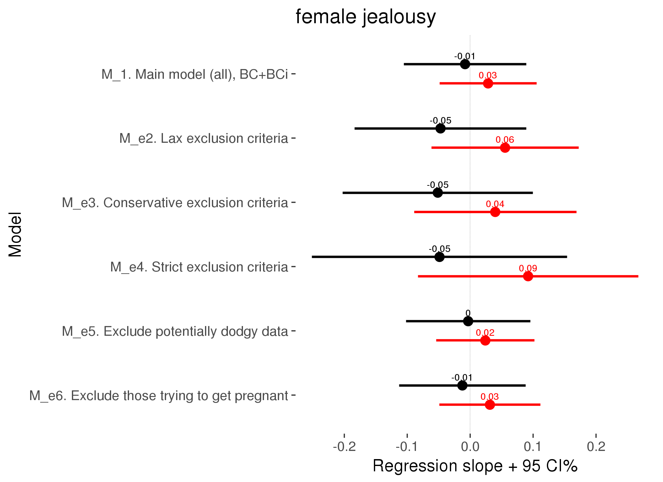
M_p: Predictors
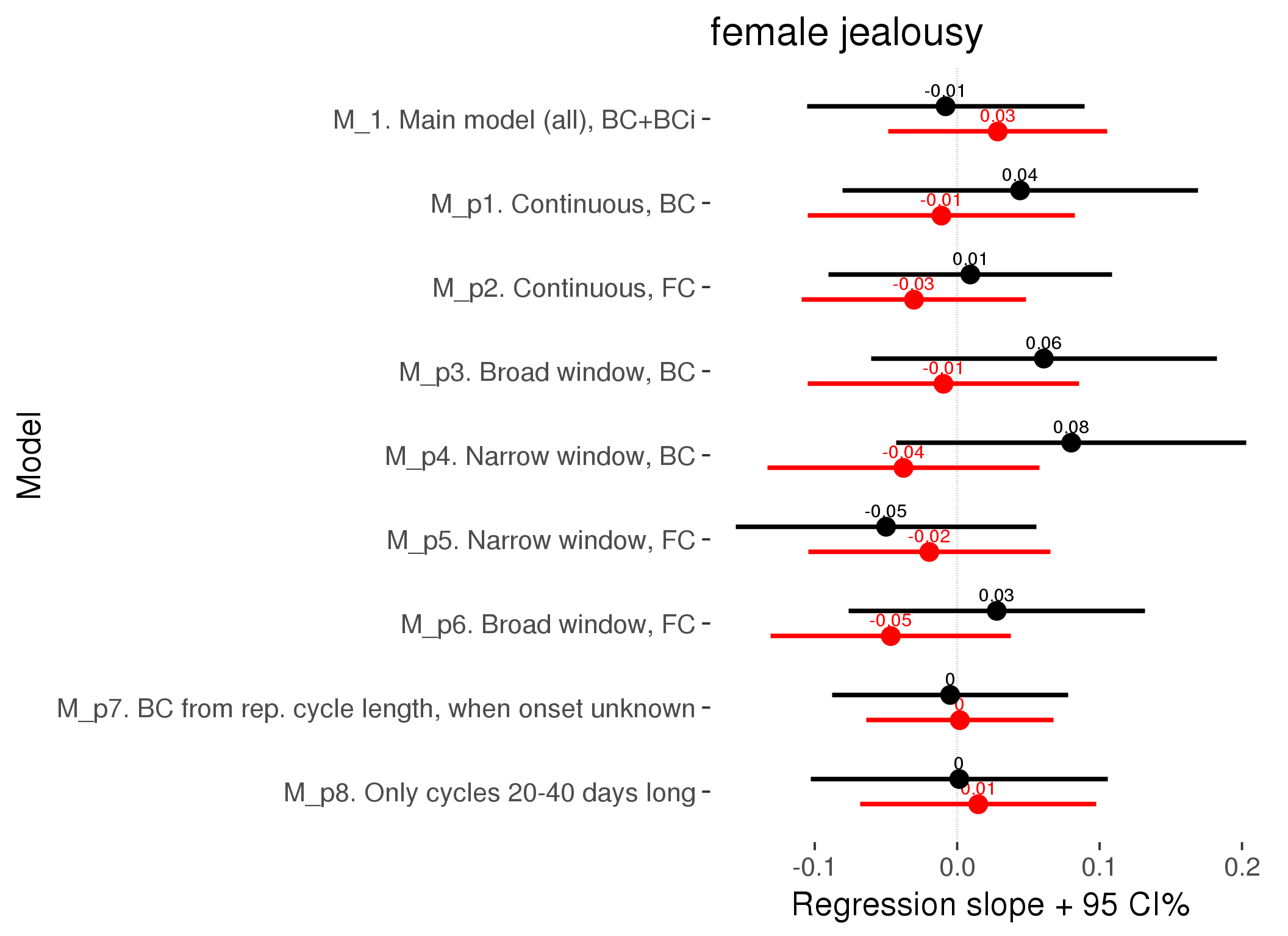
M_c: Covariates, controls, autocorrelation
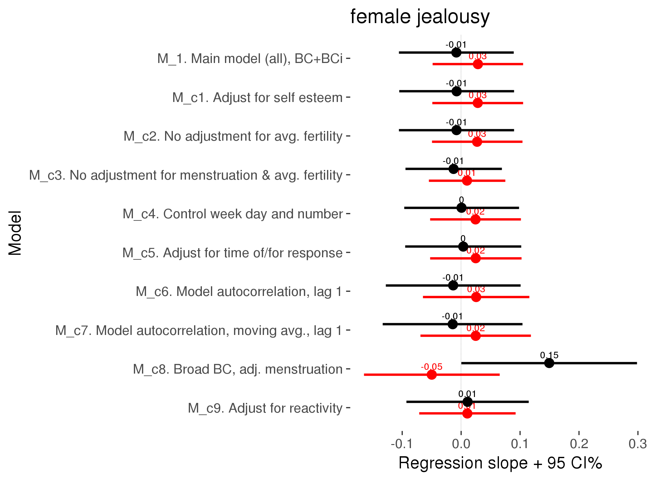
Linear mixed model fit by REML ['lmerMod']
REML criterion at convergence: 49896
Scaled residuals:
Min 1Q Median 3Q Max
-3.588 -0.538 -0.136 0.445 7.369
Random effects:
Groups Name Variance Std.Dev.
person (Intercept) 0.2892 0.538
Xr.2 s(days_filled_out):includedhorm_contra 0.0215 0.147
Xr.1 s(days_filled_out):includedcycling 0.0000 0.000
Xr.0 s(day_number):includedhorm_contra 0.0000 0.000
Xr s(day_number):includedcycling 0.0120 0.109
Residual 0.4033 0.635
Number of obs: 24379, groups: person, 1054; Xr.2, 8; Xr.1, 8; Xr.0, 8; Xr, 8
Fixed effects:
Estimate Std. Error t value
X(Intercept) 1.65275 0.04697 35.2
Xincludedhorm_contra 0.03319 0.03878 0.9
Xmenstruationpre 0.01427 0.02027 0.7
Xmenstruationyes 0.02221 0.01947 1.1
Xfertile 0.01052 0.04173 0.3
Xfertile_mean -0.07992 0.21412 -0.4
Xincludedhorm_contra:menstruationpre 0.01162 0.02600 0.4
Xincludedhorm_contra:menstruationyes -0.00151 0.02548 -0.1
Xincludedhorm_contra:fertile 0.01094 0.05284 0.2
Xs(day_number):includedcyclingFx1 0.05512 0.04666 1.2
Xs(day_number):includedhorm_contraFx1 0.06007 0.02846 2.1
Xs(days_filled_out):includedcyclingFx1 -0.03726 0.03373 -1.1
Xs(days_filled_out):includedhorm_contraFx1 0.00572 0.04817 0.1
Family: gaussian
Link function: identity
Formula:
female_jealousy ~ included + menstruation + fertile + fertile_mean +
s(day_number, by = included) + s(days_filled_out, by = included) +
included:menstruation + included:fertile
Parametric coefficients:
Estimate Std. Error t value Pr(>|t|)
(Intercept) 1.65275 0.04697 35.19 <2e-16 ***
includedhorm_contra 0.03319 0.03878 0.86 0.39
menstruationpre 0.01427 0.02027 0.70 0.48
menstruationyes 0.02221 0.01947 1.14 0.25
fertile 0.01052 0.04173 0.25 0.80
fertile_mean -0.07992 0.21412 -0.37 0.71
includedhorm_contra:menstruationpre 0.01162 0.02600 0.45 0.65
includedhorm_contra:menstruationyes -0.00151 0.02548 -0.06 0.95
includedhorm_contra:fertile 0.01094 0.05284 0.21 0.84
---
Signif. codes: 0 '***' 0.001 '**' 0.01 '*' 0.05 '.' 0.1 ' ' 1
Approximate significance of smooth terms:
edf Ref.df F p-value
s(day_number):includedcycling 3.05 3.05 7.80 0.000031 ***
s(day_number):includedhorm_contra 1.00 1.00 4.45 0.035 *
s(days_filled_out):includedcycling 1.00 1.00 1.22 0.269
s(days_filled_out):includedhorm_contra 3.94 3.94 6.84 0.000034 ***
---
Signif. codes: 0 '***' 0.001 '**' 0.01 '*' 0.05 '.' 0.1 ' ' 1
R-sq.(adj) = 0.00147
lmer.REML = 49895 Scale est. = 0.40333 n = 24379
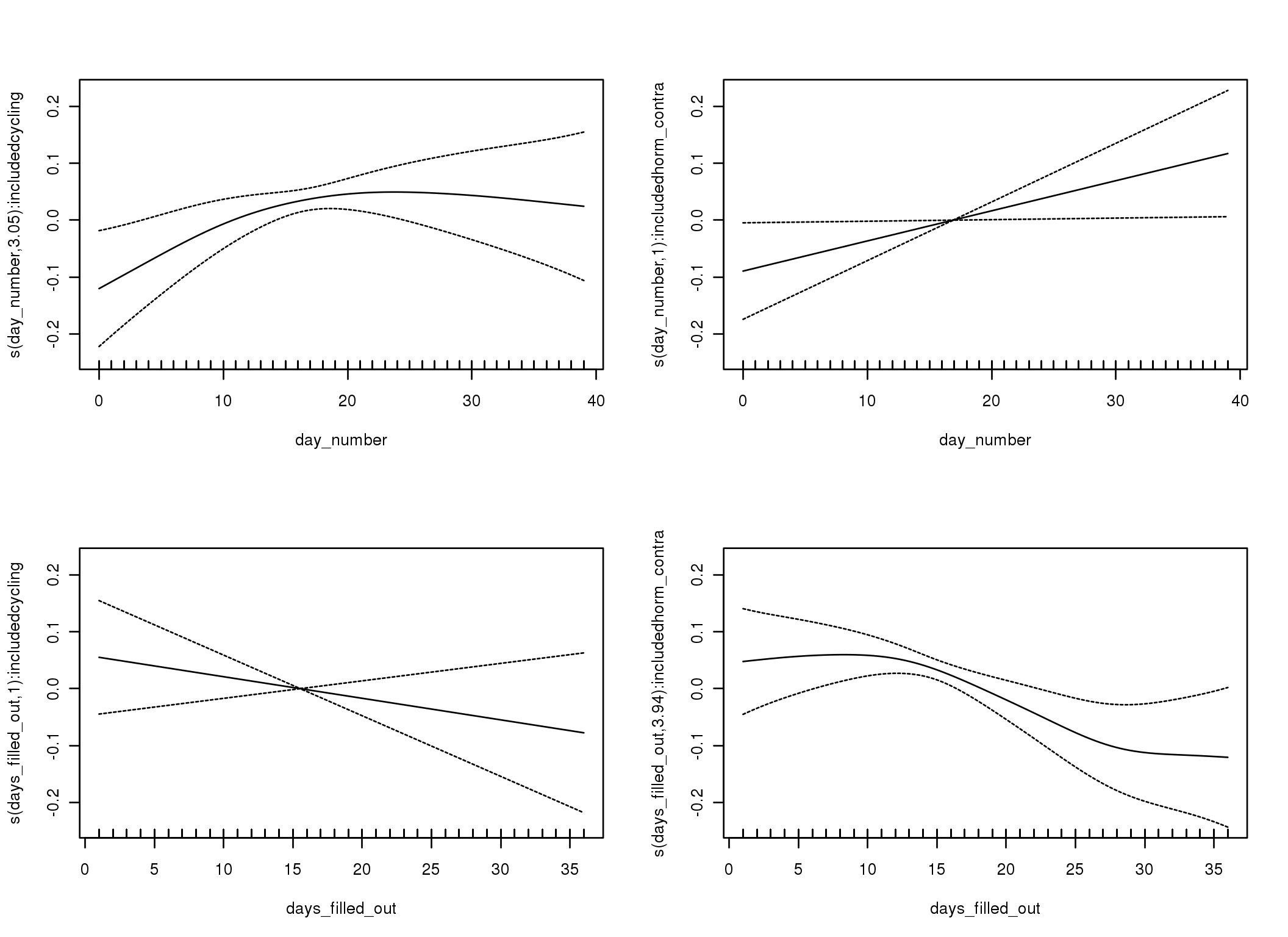
Linear mixed-effects model fit by REML
Data: diary
AIC BIC logLik
53538 53637 -26757
Random effects:
Formula: ~1 | person
(Intercept) Residual
StdDev: 0.5316 0.6433
Correlation Structure: ARMA(1,0)
Formula: ~day_number | person
Parameter estimate(s):
Phi1
0.2357
Fixed effects: female_jealousy ~ included * (menstruation + fertile) + fertile_mean
Value Std.Error DF t-value p-value
(Intercept) 1.6581 0.04744 25622 34.95 0.0000
includedhorm_contra 0.0384 0.03904 1051 0.98 0.3251
menstruationpre 0.0073 0.02198 25622 0.33 0.7385
menstruationyes 0.0087 0.02056 25622 0.42 0.6737
fertile 0.0255 0.04604 25622 0.55 0.5794
fertile_mean -0.0947 0.21745 1051 -0.44 0.6632
includedhorm_contra:menstruationpre 0.0147 0.02823 25622 0.52 0.6029
includedhorm_contra:menstruationyes 0.0131 0.02684 25622 0.49 0.6265
includedhorm_contra:fertile -0.0135 0.05826 25622 -0.23 0.8167
Correlation:
(Intr) incld_ mnstrtnp mnstrtny fertil frtl_m inclddhrm_cntr:mnstrtnp
includedhorm_contra -0.476
menstruationpre -0.177 0.222
menstruationyes -0.173 0.216 0.401
fertile -0.170 0.280 0.438 0.367
fertile_mean -0.769 -0.026 -0.008 -0.006 -0.077
includedhorm_contra:menstruationpre 0.145 -0.278 -0.779 -0.312 -0.340 -0.004
includedhorm_contra:menstruationyes 0.139 -0.264 -0.307 -0.766 -0.281 -0.003 0.386
includedhorm_contra:fertile 0.171 -0.354 -0.346 -0.290 -0.787 0.013 0.437
inclddhrm_cntr:mnstrtny
includedhorm_contra
menstruationpre
menstruationyes
fertile
fertile_mean
includedhorm_contra:menstruationpre
includedhorm_contra:menstruationyes
includedhorm_contra:fertile 0.362
Standardized Within-Group Residuals:
Min Q1 Med Q3 Max
-3.4563 -0.5396 -0.1478 0.4433 7.2050
Number of Observations: 26682
Number of Groups: 1054
Linear mixed-effects model fit by REML
Data: diary
AIC BIC logLik
53461 53568 -26718
Random effects:
Formula: ~1 | person
(Intercept) Residual
StdDev: 0.5262 0.6463
Correlation Structure: ARMA(1,1)
Formula: ~day_number | person
Parameter estimate(s):
Phi1 Theta1
0.5269 -0.3083
Fixed effects: female_jealousy ~ included * (menstruation + fertile) + fertile_mean
Value Std.Error DF t-value p-value
(Intercept) 1.6596 0.04748 25622 34.95 0.0000
includedhorm_contra 0.0379 0.03911 1051 0.97 0.3333
menstruationpre 0.0035 0.02238 25622 0.16 0.8747
menstruationyes 0.0061 0.02103 25622 0.29 0.7716
fertile 0.0247 0.04787 25622 0.52 0.6053
fertile_mean -0.1005 0.21784 1051 -0.46 0.6448
includedhorm_contra:menstruationpre 0.0200 0.02875 25622 0.70 0.4863
includedhorm_contra:menstruationyes 0.0144 0.02740 25622 0.53 0.5993
includedhorm_contra:fertile -0.0143 0.06054 25622 -0.24 0.8132
Correlation:
(Intr) incld_ mnstrtnp mnstrtny fertil frtl_m inclddhrm_cntr:mnstrtnp
includedhorm_contra -0.477
menstruationpre -0.179 0.223
menstruationyes -0.177 0.220 0.410
fertile -0.172 0.286 0.414 0.359
fertile_mean -0.768 -0.027 -0.006 -0.005 -0.081
includedhorm_contra:menstruationpre 0.146 -0.279 -0.778 -0.319 -0.321 -0.004
includedhorm_contra:menstruationyes 0.142 -0.270 -0.315 -0.768 -0.275 -0.003 0.397
includedhorm_contra:fertile 0.174 -0.361 -0.327 -0.284 -0.787 0.014 0.413
inclddhrm_cntr:mnstrtny
includedhorm_contra
menstruationpre
menstruationyes
fertile
fertile_mean
includedhorm_contra:menstruationpre
includedhorm_contra:menstruationyes
includedhorm_contra:fertile 0.353
Standardized Within-Group Residuals:
Min Q1 Med Q3 Max
-3.3673 -0.5420 -0.1551 0.4509 7.1285
Number of Observations: 26682
Number of Groups: 1054
M_d: Other designs
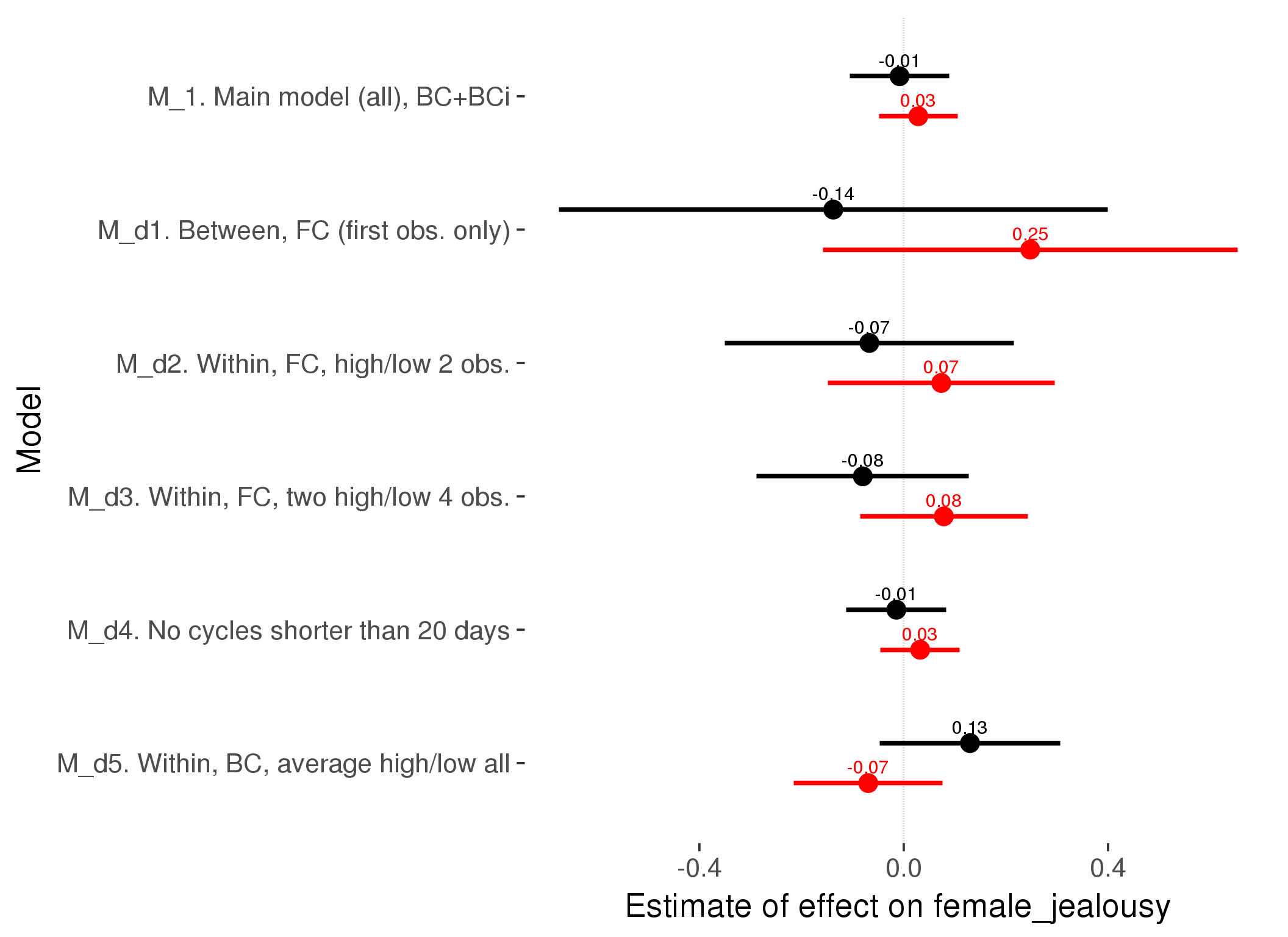
M_m1: Moderation by contraceptive method
Based on the sample with lax exclusion criteria. Users who used any hormonal contraception are classified as hormonal, users who use any awareness-based methods (counting, temperature-based) are classified as ‘fertility-awareness’, women who don’t fall into the before groups and use condoms, pessars, coitus interruptus etc. are classified as ‘barrie or abstinence’. Women who don’t use contraception or use other methods such as sterilisation are excluded from this analysis.
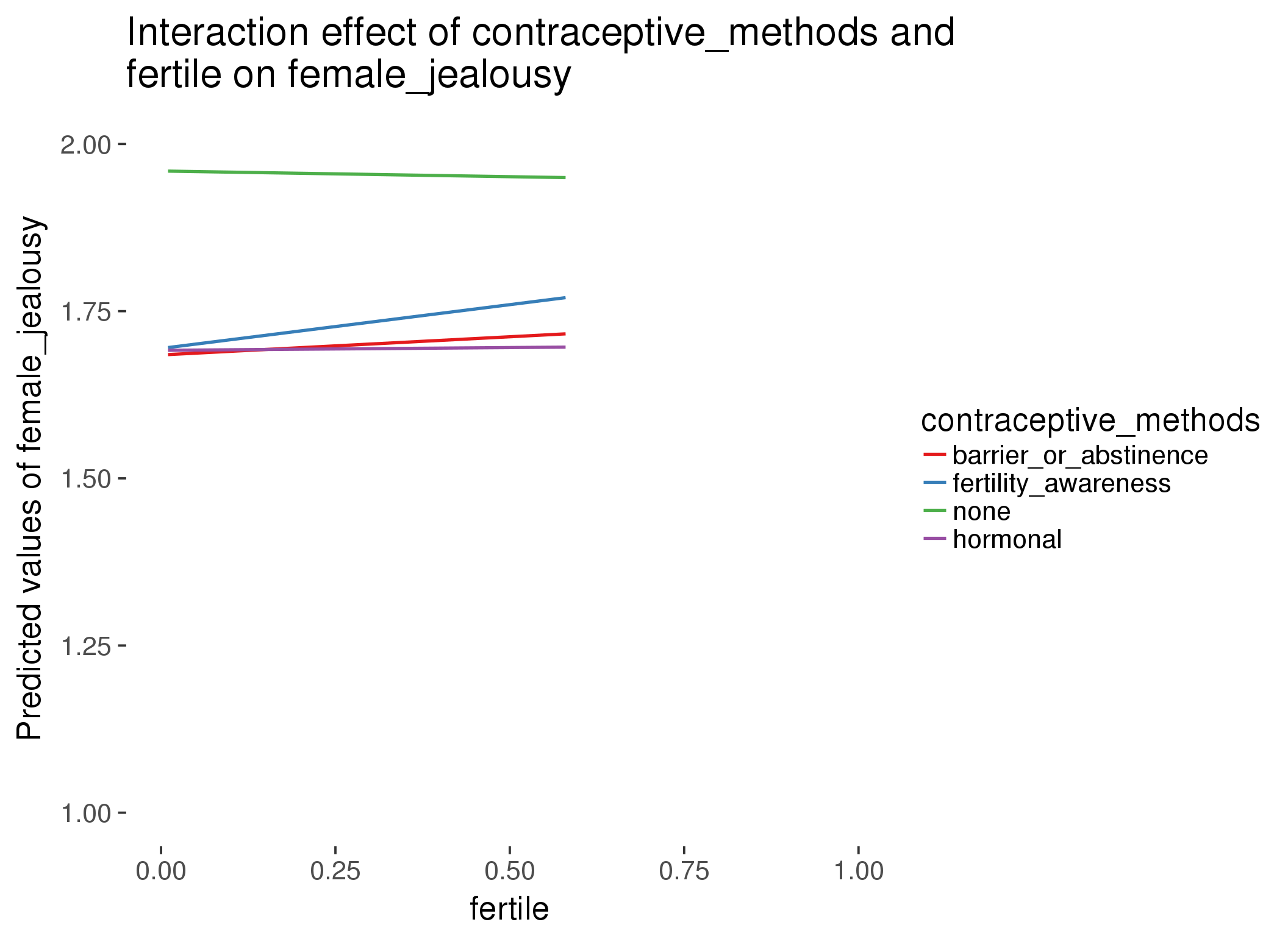
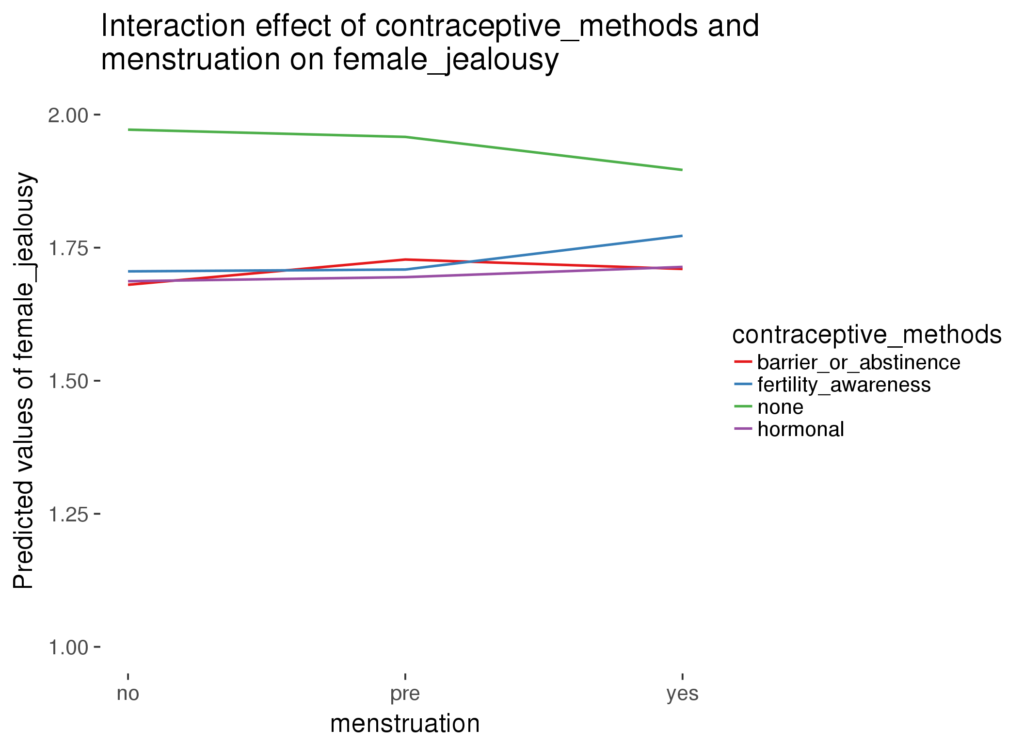
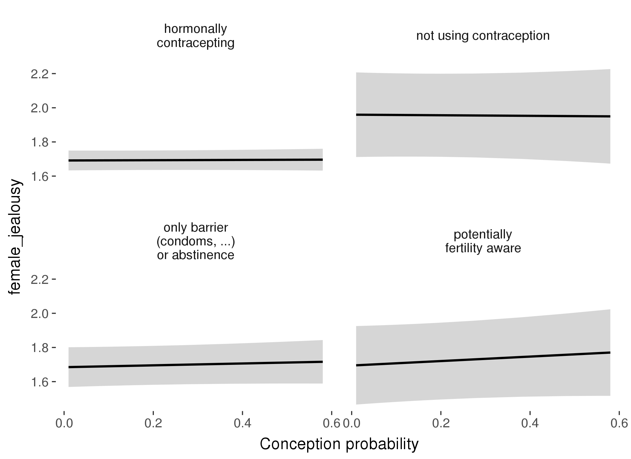
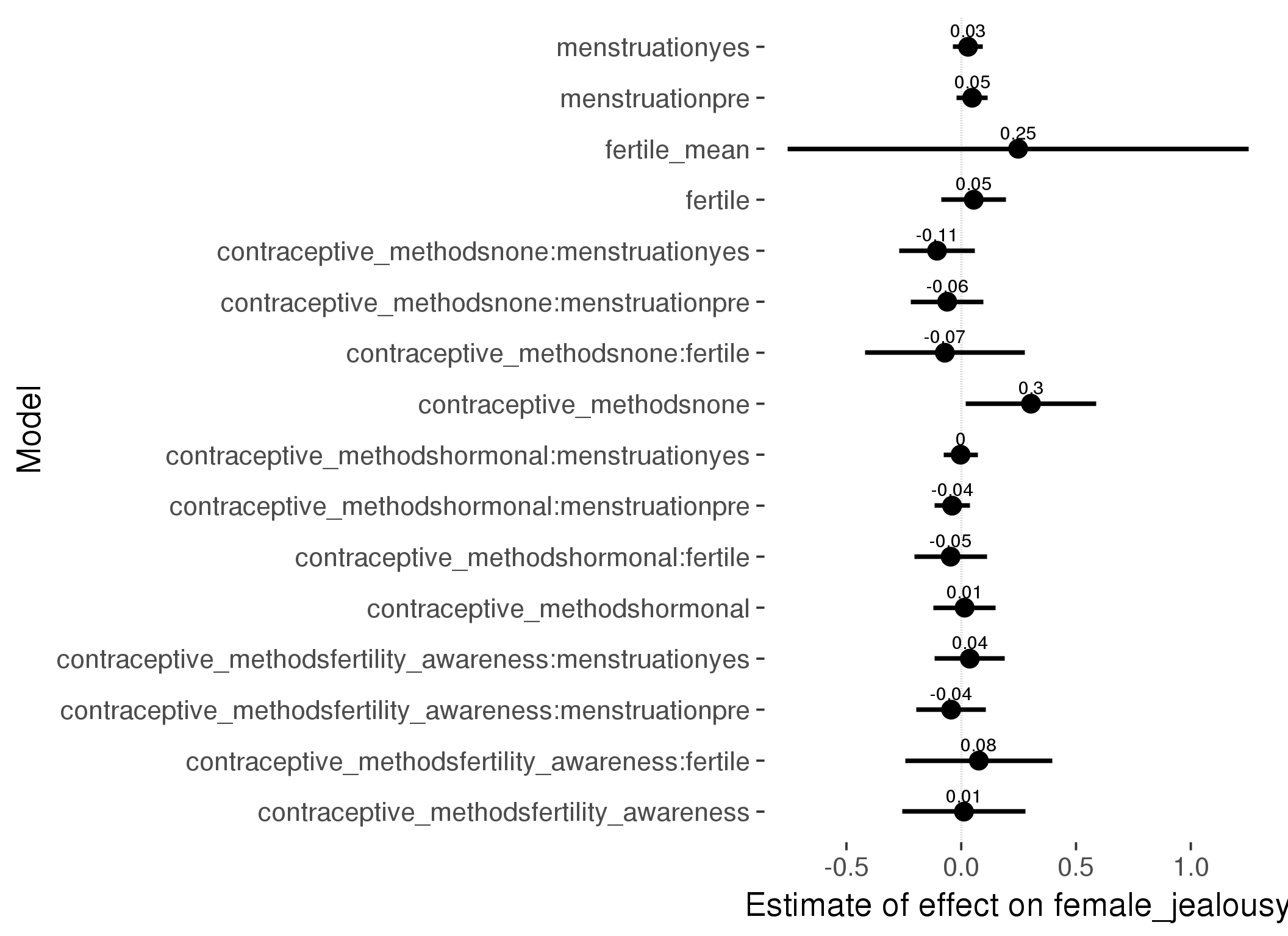
Linear mixed model fit by REML ['lmerMod']
Formula: female_jealousy ~ fertile_mean + (1 | person) + contraceptive_methods +
fertile + menstruation + fertile:contraceptive_methods + menstruation:contraceptive_methods
Data: diary
Subset: !is.na(included_lax) & contraceptive_method != "other"
REML criterion at convergence: 35174
Scaled residuals:
Min 1Q Median 3Q Max
-3.600 -0.546 -0.129 0.460 7.178
Random effects:
Groups Name Variance Std.Dev.
person (Intercept) 0.303 0.550
Residual 0.418 0.647
Number of obs: 17028, groups: person, 513
Fixed effects:
Estimate Std. Error t value
(Intercept) 1.62726 0.10533 15.45
fertile_mean 0.24785 0.51252 0.48
contraceptive_methodsfertility_awareness 0.01177 0.13655 0.09
contraceptive_methodsnone 0.30398 0.14472 2.10
contraceptive_methodshormonal 0.01479 0.06886 0.21
fertile 0.05442 0.07218 0.75
menstruationpre 0.04745 0.03486 1.36
menstruationyes 0.02974 0.03330 0.89
contraceptive_methodsfertility_awareness:fertile 0.07655 0.16391 0.47
contraceptive_methodsnone:fertile -0.07141 0.17744 -0.40
contraceptive_methodshormonal:fertile -0.04614 0.08063 -0.57
contraceptive_methodsfertility_awareness:menstruationpre -0.04400 0.07721 -0.57
contraceptive_methodsnone:menstruationpre -0.06108 0.08073 -0.76
contraceptive_methodshormonal:menstruationpre -0.03980 0.03926 -1.01
contraceptive_methodsfertility_awareness:menstruationyes 0.03712 0.07760 0.48
contraceptive_methodsnone:menstruationyes -0.10542 0.08441 -1.25
contraceptive_methodshormonal:menstruationyes -0.00285 0.03797 -0.08
refitting model(s) with ML (instead of REML)
| Df | AIC | BIC | logLik | deviance | Chisq | Chi Df | Pr(>Chisq) | |
|---|---|---|---|---|---|---|---|---|
| add_main | 13 | 35140 | 35241 | -17557 | 35114 | NA | NA | NA |
| by_method | 19 | 35149 | 35296 | -17555 | 35111 | 3.228 | 6 | 0.7798 |
M_m2: Moderation by participant age
model %>%
test_moderator("age_group", diary, xlevels = 5)refitting model(s) with ML (instead of REML)
| Df | AIC | BIC | logLik | deviance | Chisq | Chi Df | Pr(>Chisq) | |
|---|---|---|---|---|---|---|---|---|
| with_main | 19 | 54499 | 54654 | -27230 | 54461 | NA | NA | NA |
| with_mod | 27 | 54500 | 54721 | -27223 | 54446 | 14.53 | 8 | 0.06901 |
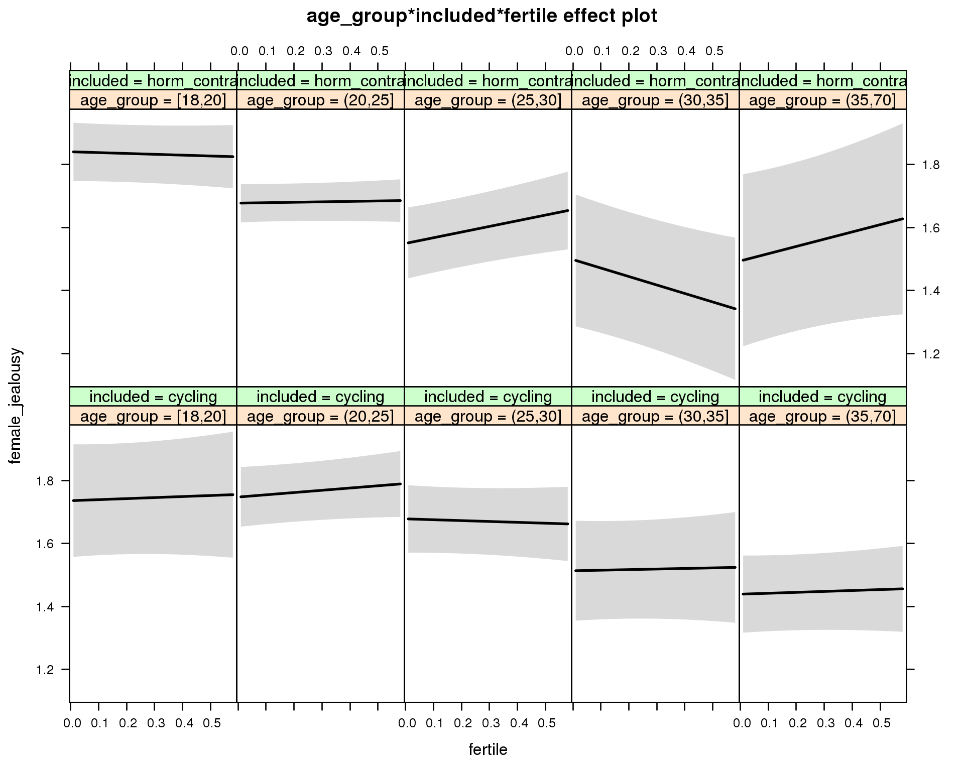
Linear mixed model fit by REML ['lmerMod']
Formula: female_jealousy ~ menstruation + fertile_mean + (1 | person) +
age_group + included + fertile + menstruation:included +
age_group:included + age_group:fertile + included:fertile + age_group:included:fertile
Data: diary
REML criterion at convergence: 54542
Scaled residuals:
Min 1Q Median 3Q Max
-3.610 -0.540 -0.136 0.445 7.269
Random effects:
Groups Name Variance Std.Dev.
person (Intercept) 0.280 0.529
Residual 0.406 0.637
Number of obs: 26682, groups: person, 1054
Fixed effects:
Estimate Std. Error t value
(Intercept) 1.75554 0.09643 18.21
menstruationpre 0.00766 0.01945 0.39
menstruationyes 0.00985 0.01833 0.54
fertile_mean -0.13125 0.21190 -0.62
age_group(20,25] 0.01153 0.10322 0.11
age_group(25,30] -0.05766 0.10624 -0.54
age_group(30,35] -0.22240 0.12190 -1.82
age_group(35,70] -0.29669 0.11040 -2.69
includedhorm_contra 0.10030 0.10340 0.97
fertile 0.03290 0.11219 0.29
menstruationpre:includedhorm_contra 0.01306 0.02497 0.52
menstruationyes:includedhorm_contra 0.00984 0.02403 0.41
age_group(20,25]:includedhorm_contra -0.17459 0.11771 -1.48
age_group(25,30]:includedhorm_contra -0.23317 0.12965 -1.80
age_group(30,35]:includedhorm_contra -0.11973 0.16882 -0.71
age_group(35,70]:includedhorm_contra -0.04976 0.18424 -0.27
age_group(20,25]:fertile 0.03867 0.12428 0.31
age_group(25,30]:fertile -0.06046 0.12810 -0.47
age_group(30,35]:fertile -0.01456 0.14837 -0.10
age_group(35,70]:fertile -0.00368 0.13389 -0.03
includedhorm_contra:fertile -0.05975 0.12443 -0.48
age_group(20,25]:includedhorm_contra:fertile 0.00204 0.13921 0.01
age_group(25,30]:includedhorm_contra:fertile 0.26695 0.15427 1.73
age_group(30,35]:includedhorm_contra:fertile -0.22785 0.19912 -1.14
age_group(35,70]:includedhorm_contra:fertile 0.26079 0.22622 1.15
M_m3: Moderation by weekend
model %>%
test_moderator("weekend", diary, xlevels = 2) refitting model(s) with ML (instead of REML)
| Df | AIC | BIC | logLik | deviance | Chisq | Chi Df | Pr(>Chisq) | |
|---|---|---|---|---|---|---|---|---|
| with_main | 13 | 54523 | 54629 | -27248 | 54497 | NA | NA | NA |
| with_mod | 15 | 54527 | 54650 | -27248 | 54497 | 0.0393 | 2 | 0.9805 |
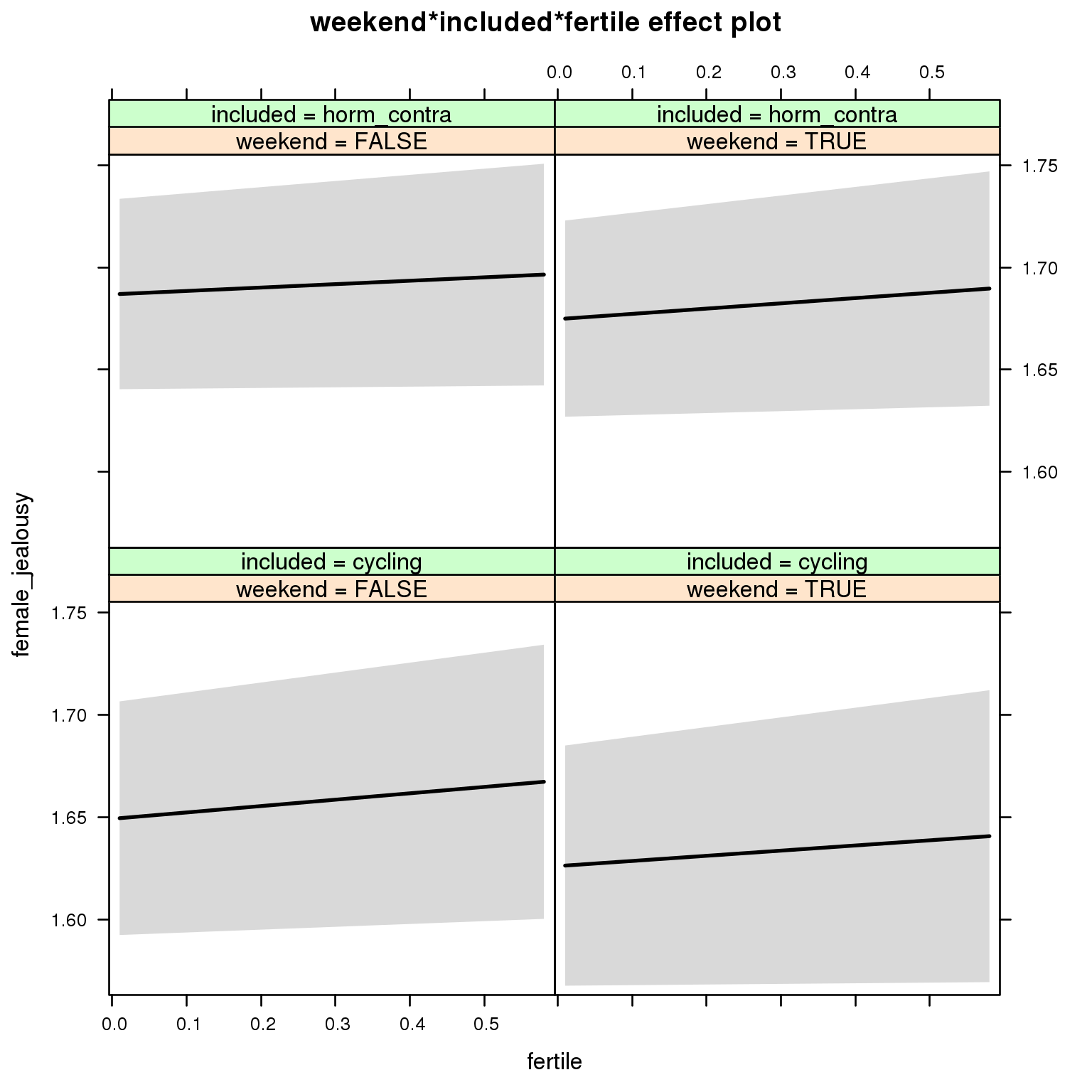
Linear mixed model fit by REML ['lmerMod']
Formula: female_jealousy ~ menstruation + fertile_mean + (1 | person) +
weekend + included + fertile + menstruation:included + weekend:included +
weekend:fertile + included:fertile + weekend:included:fertile
Data: diary
REML criterion at convergence: 54567
Scaled residuals:
Min 1Q Median 3Q Max
-3.626 -0.541 -0.134 0.444 7.300
Random effects:
Groups Name Variance Std.Dev.
person (Intercept) 0.289 0.537
Residual 0.406 0.637
Number of obs: 26682, groups: person, 1054
Fixed effects:
Estimate Std. Error t value
(Intercept) 1.66577 0.04714 35.3
menstruationpre 0.00779 0.01945 0.4
menstruationyes 0.01018 0.01832 0.6
fertile_mean -0.11333 0.21362 -0.5
weekendTRUE -0.02313 0.01694 -1.4
includedhorm_contra 0.03319 0.03922 0.8
fertile 0.03123 0.04773 0.7
menstruationpre:includedhorm_contra 0.01433 0.02496 0.6
menstruationyes:includedhorm_contra 0.01055 0.02402 0.4
weekendTRUE:includedhorm_contra 0.01101 0.02181 0.5
weekendTRUE:fertile -0.00597 0.06572 -0.1
includedhorm_contra:fertile -0.01456 0.06065 -0.2
weekendTRUE:includedhorm_contra:fertile 0.01508 0.08359 0.2
M_m4: Moderation by weekday
model %>%
test_moderator("weekday", diary, xlevels = 7)refitting model(s) with ML (instead of REML)
| Df | AIC | BIC | logLik | deviance | Chisq | Chi Df | Pr(>Chisq) | |
|---|---|---|---|---|---|---|---|---|
| with_main | 23 | 54497 | 54685 | -27225 | 54451 | NA | NA | NA |
| with_mod | 35 | 54517 | 54804 | -27223 | 54447 | 3.76 | 12 | 0.9874 |
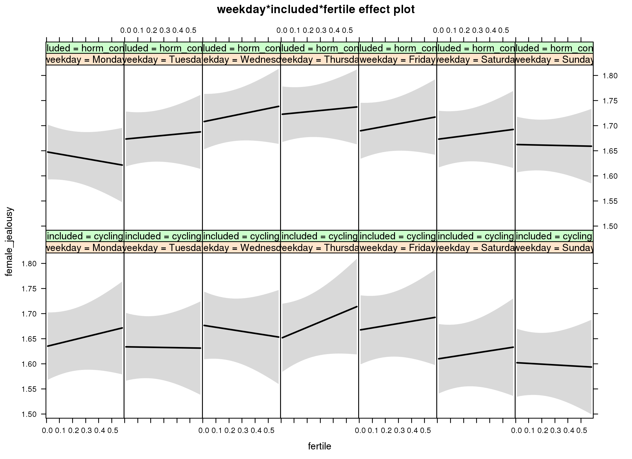
Linear mixed model fit by REML ['lmerMod']
Formula: female_jealousy ~ menstruation + fertile_mean + (1 | person) +
weekday + included + fertile + menstruation:included + weekday:included +
weekday:fertile + included:fertile + weekday:included:fertile
Data: diary
REML criterion at convergence: 54606
Scaled residuals:
Min 1Q Median 3Q Max
-3.611 -0.540 -0.135 0.444 7.274
Random effects:
Groups Name Variance Std.Dev.
person (Intercept) 0.289 0.538
Residual 0.405 0.637
Number of obs: 26682, groups: person, 1054
Fixed effects:
Estimate Std. Error t value
(Intercept) 1.649957 0.050649 32.6
menstruationpre 0.007628 0.019437 0.4
menstruationyes 0.010089 0.018315 0.6
fertile_mean -0.105144 0.213688 -0.5
weekdayTuesday -0.000734 0.030304 0.0
weekdayWednesday 0.042232 0.030254 1.4
weekdayThursday 0.016254 0.030599 0.5
weekdayFriday 0.032597 0.031116 1.0
weekdaySaturday -0.024948 0.031427 -0.8
weekdaySunday -0.032302 0.030370 -1.1
includedhorm_contra 0.008723 0.045788 0.2
fertile 0.063501 0.085354 0.7
menstruationpre:includedhorm_contra 0.013710 0.024954 0.5
menstruationyes:includedhorm_contra 0.009882 0.024011 0.4
weekdayTuesday:includedhorm_contra 0.026016 0.038931 0.7
weekdayWednesday:includedhorm_contra 0.017495 0.039059 0.4
weekdayThursday:includedhorm_contra 0.058341 0.039431 1.5
weekdayFriday:includedhorm_contra 0.008831 0.039975 0.2
weekdaySaturday:includedhorm_contra 0.049929 0.040439 1.2
weekdaySunday:includedhorm_contra 0.046812 0.039200 1.2
weekdayTuesday:fertile -0.067991 0.117494 -0.6
weekdayWednesday:fertile -0.104063 0.118042 -0.9
weekdayThursday:fertile 0.045166 0.119731 0.4
weekdayFriday:fertile -0.019936 0.119938 -0.2
weekdaySaturday:fertile -0.023075 0.121534 -0.2
weekdaySunday:fertile -0.078521 0.118110 -0.7
includedhorm_contra:fertile -0.108971 0.109179 -1.0
weekdayTuesday:includedhorm_contra:fertile 0.138220 0.149961 0.9
weekdayWednesday:includedhorm_contra:fertile 0.202596 0.151141 1.3
weekdayThursday:includedhorm_contra:fertile 0.025708 0.152355 0.2
weekdayFriday:includedhorm_contra:fertile 0.113214 0.152836 0.7
weekdaySaturday:includedhorm_contra:fertile 0.102230 0.155037 0.7
weekdaySunday:includedhorm_contra:fertile 0.118228 0.150870 0.8
M_m5: Moderation by exclusion threshold
model %>%
test_moderator("included_levels", diary, xlevels = 4)refitting model(s) with ML (instead of REML)
| Df | AIC | BIC | logLik | deviance | Chisq | Chi Df | Pr(>Chisq) | |
|---|---|---|---|---|---|---|---|---|
| with_main | 17 | 54525 | 54664 | -27245 | 54491 | NA | NA | NA |
| with_mod | 23 | 54534 | 54722 | -27244 | 54488 | 2.458 | 6 | 0.8731 |
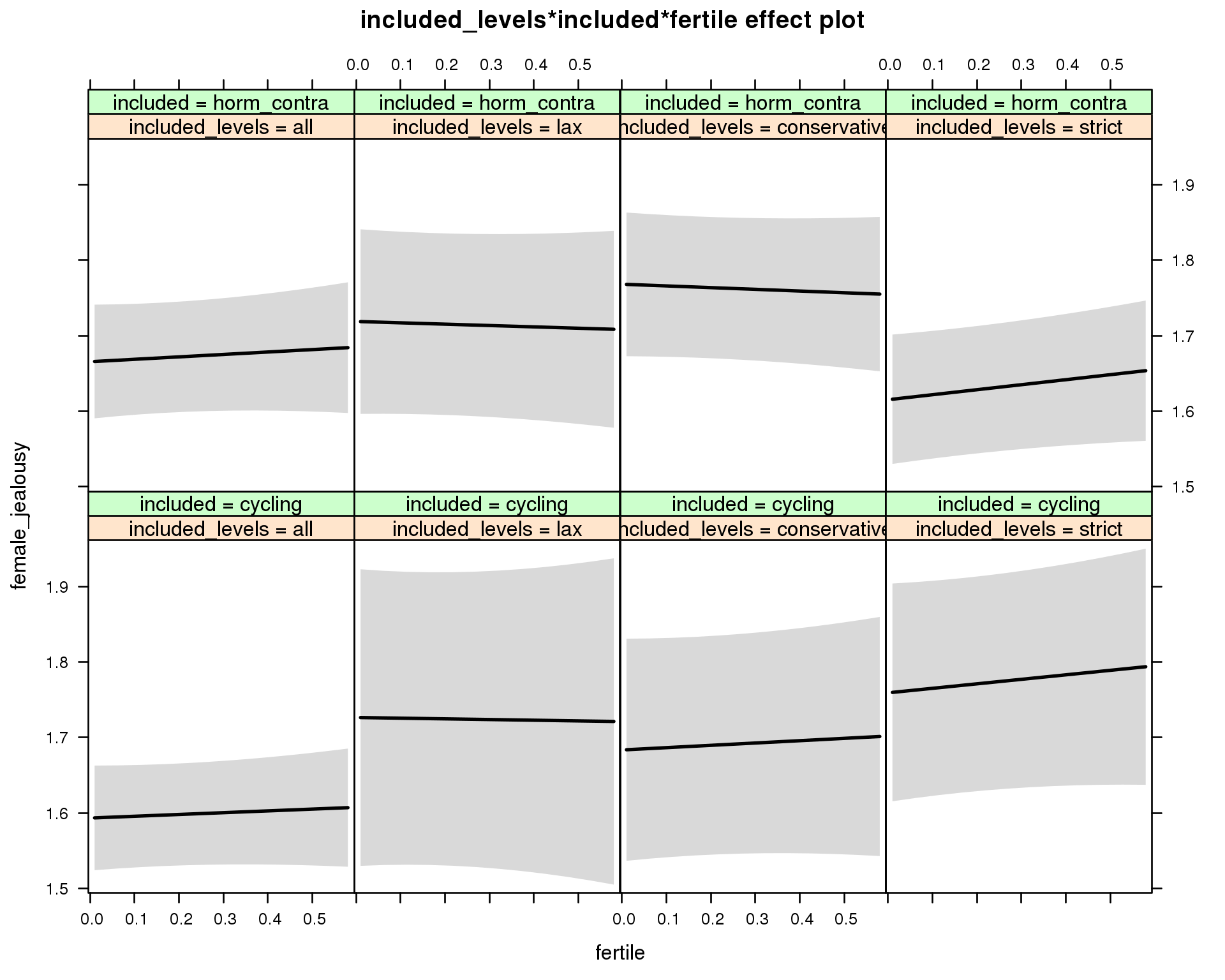
Linear mixed model fit by REML ['lmerMod']
Formula: female_jealousy ~ menstruation + fertile_mean + (1 | person) +
included_levels + included + fertile + menstruation:included +
included_levels:included + included_levels:fertile + included:fertile +
included_levels:included:fertile
Data: diary
REML criterion at convergence: 54576
Scaled residuals:
Min 1Q Median 3Q Max
-3.615 -0.541 -0.131 0.443 7.292
Random effects:
Groups Name Variance Std.Dev.
person (Intercept) 0.287 0.536
Residual 0.406 0.637
Number of obs: 26682, groups: person, 1054
Fixed effects:
Estimate Std. Error t value
(Intercept) 1.61134 0.05166 31.19
menstruationpre 0.00733 0.01947 0.38
menstruationyes 0.01020 0.01833 0.56
fertile_mean -0.12252 0.21504 -0.57
included_levelslax 0.13329 0.10641 1.25
included_levelsconservative 0.09024 0.08303 1.09
included_levelsstrict 0.16597 0.08170 2.03
includedhorm_contra 0.06794 0.05333 1.27
fertile 0.02375 0.04961 0.48
menstruationpre:includedhorm_contra 0.01466 0.02500 0.59
menstruationyes:includedhorm_contra 0.01048 0.02405 0.44
included_levelslax:includedhorm_contra -0.07993 0.12949 -0.62
included_levelsconservative:includedhorm_contra 0.01249 0.10367 0.12
included_levelsstrict:includedhorm_contra -0.21634 0.10037 -2.16
included_levelslax:fertile -0.03279 0.12114 -0.27
included_levelsconservative:fertile 0.00704 0.09048 0.08
included_levelsstrict:fertile 0.03589 0.09054 0.40
includedhorm_contra:fertile 0.00843 0.07580 0.11
included_levelslax:includedhorm_contra:fertile -0.01731 0.14782 -0.12
included_levelsconservative:includedhorm_contra:fertile -0.06182 0.11766 -0.53
included_levelsstrict:includedhorm_contra:fertile -0.00170 0.11585 -0.01
M_m6: Moderation by cycle length
model %>%
test_moderator("cycle_length_groups", diary, xlevels = 4)refitting model(s) with ML (instead of REML)
| Df | AIC | BIC | logLik | deviance | Chisq | Chi Df | Pr(>Chisq) | |
|---|---|---|---|---|---|---|---|---|
| with_main | 17 | 54527 | 54666 | -27247 | 54493 | NA | NA | NA |
| with_mod | 23 | 54529 | 54717 | -27241 | 54483 | 10.3 | 6 | 0.1125 |
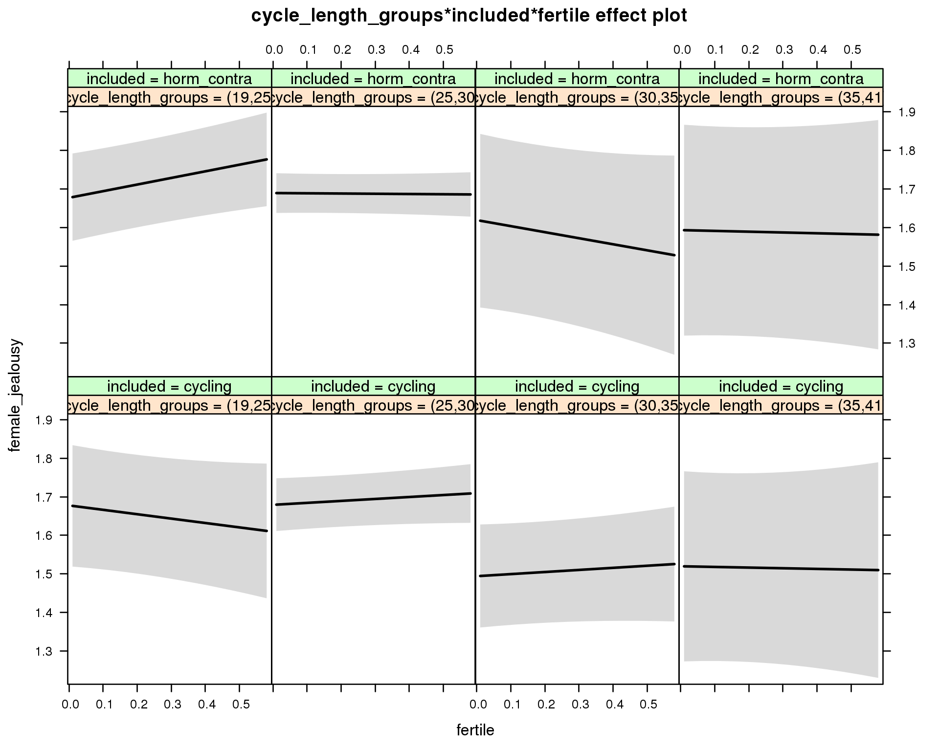
Linear mixed model fit by REML ['lmerMod']
Formula: female_jealousy ~ menstruation + fertile_mean + (1 | person) +
cycle_length_groups + included + fertile + menstruation:included +
cycle_length_groups:included + cycle_length_groups:fertile +
included:fertile + cycle_length_groups:included:fertile
Data: diary
REML criterion at convergence: 54563
Scaled residuals:
Min 1Q Median 3Q Max
-3.612 -0.542 -0.135 0.441 7.295
Random effects:
Groups Name Variance Std.Dev.
person (Intercept) 0.288 0.537
Residual 0.406 0.637
Number of obs: 26682, groups: person, 1054
Fixed effects:
Estimate Std. Error t value
(Intercept) 1.70659 0.08924 19.12
menstruationpre 0.00891 0.01947 0.46
menstruationyes 0.01312 0.01846 0.71
fertile_mean -0.18910 0.21613 -0.87
cycle_length_groups(25,30] 0.00160 0.08770 0.02
cycle_length_groups(30,35] -0.18341 0.10552 -1.74
cycle_length_groups(35,41] -0.15772 0.14952 -1.05
includedhorm_contra -0.00353 0.09967 -0.04
fertile -0.11386 0.10357 -1.10
menstruationpre:includedhorm_contra 0.01266 0.02499 0.51
menstruationyes:includedhorm_contra 0.00463 0.02416 0.19
cycle_length_groups(25,30]:includedhorm_contra 0.01066 0.10829 0.10
cycle_length_groups(30,35]:includedhorm_contra 0.12549 0.16625 0.75
cycle_length_groups(35,41]:includedhorm_contra 0.07389 0.21230 0.35
cycle_length_groups(25,30]:fertile 0.16460 0.11112 1.48
cycle_length_groups(30,35]:fertile 0.16796 0.13157 1.28
cycle_length_groups(35,41]:fertile 0.09683 0.18584 0.52
includedhorm_contra:fertile 0.28539 0.12227 2.33
cycle_length_groups(25,30]:includedhorm_contra:fertile -0.34236 0.13165 -2.60
cycle_length_groups(30,35]:includedhorm_contra:fertile -0.49617 0.20716 -2.40
cycle_length_groups(35,41]:includedhorm_contra:fertile -0.28885 0.24472 -1.18
M_m7: Moderation by certainty about menstruation parameters
model %>%
test_moderator("certainty_menstruation", diary)refitting model(s) with ML (instead of REML)
| Df | AIC | BIC | logLik | deviance | Chisq | Chi Df | Pr(>Chisq) | |
|---|---|---|---|---|---|---|---|---|
| with_main | 13 | 54526 | 54633 | -27250 | 54500 | NA | NA | NA |
| with_mod | 15 | 54527 | 54650 | -27248 | 54497 | 3.445 | 2 | 0.1787 |
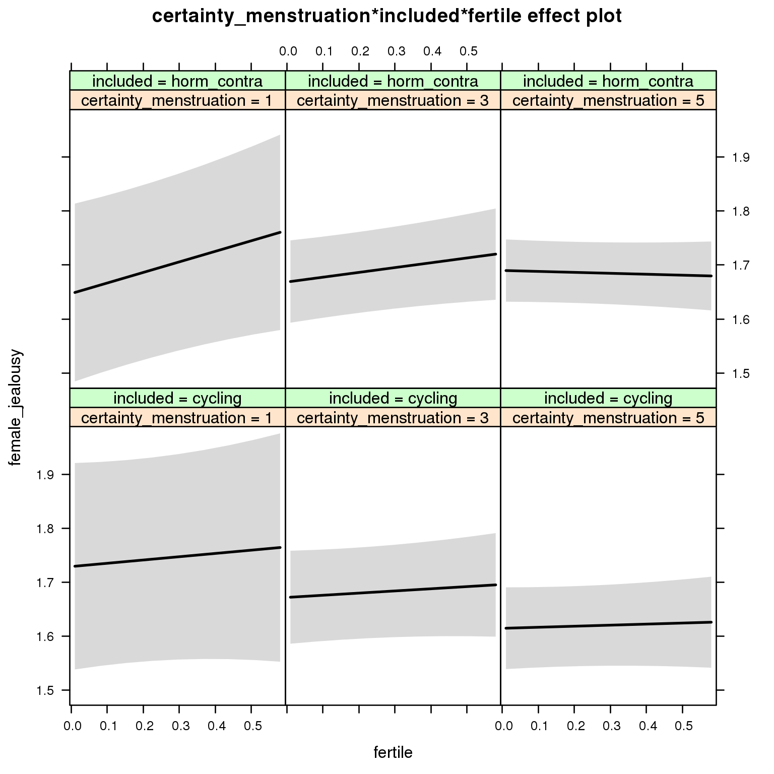
Linear mixed model fit by REML ['lmerMod']
Formula: female_jealousy ~ menstruation + fertile_mean + (1 | person) +
certainty_menstruation + included + fertile + menstruation:included +
certainty_menstruation:included + certainty_menstruation:fertile +
included:fertile + certainty_menstruation:included:fertile
Data: diary
REML criterion at convergence: 54566
Scaled residuals:
Min 1Q Median 3Q Max
-3.613 -0.542 -0.132 0.442 7.298
Random effects:
Groups Name Variance Std.Dev.
person (Intercept) 0.289 0.538
Residual 0.406 0.637
Number of obs: 26682, groups: person, 1054
Fixed effects:
Estimate Std. Error t value
(Intercept) 1.77446 0.13149 13.50
menstruationpre 0.00759 0.01946 0.39
menstruationyes 0.00971 0.01835 0.53
fertile_mean -0.11326 0.21407 -0.53
certainty_menstruation -0.02861 0.02997 -0.95
includedhorm_contra -0.12567 0.16694 -0.75
fertile 0.07112 0.15447 0.46
menstruationpre:includedhorm_contra 0.01434 0.02497 0.57
menstruationyes:includedhorm_contra 0.01029 0.02405 0.43
certainty_menstruation:includedhorm_contra 0.03930 0.03889 1.01
certainty_menstruation:fertile -0.01032 0.03619 -0.29
includedhorm_contra:fertile 0.17772 0.20078 0.89
certainty_menstruation:includedhorm_contra:fertile -0.04293 0.04641 -0.93
M_m8: Moderation by cycle regularity
model %>%
test_moderator("cycle_regularity", diary)refitting model(s) with ML (instead of REML)
| Df | AIC | BIC | logLik | deviance | Chisq | Chi Df | Pr(>Chisq) | |
|---|---|---|---|---|---|---|---|---|
| with_main | 15 | 54526 | 54649 | -27248 | 54496 | NA | NA | NA |
| with_mod | 19 | 54528 | 54684 | -27245 | 54490 | 6.288 | 4 | 0.1787 |
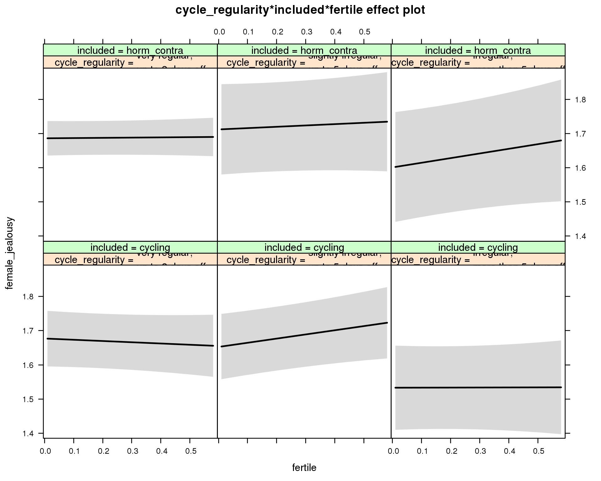
Linear mixed model fit by REML ['lmerMod']
Formula: female_jealousy ~ menstruation + fertile_mean + (1 | person) +
cycle_regularity + included + fertile + menstruation:included +
cycle_regularity:included + cycle_regularity:fertile + included:fertile +
cycle_regularity:included:fertile
Data: diary
REML criterion at convergence: 54564
Scaled residuals:
Min 1Q Median 3Q Max
-3.604 -0.542 -0.133 0.444 7.293
Random effects:
Groups Name Variance Std.Dev.
person (Intercept) 0.288 0.537
Residual 0.406 0.637
Number of obs: 26682, groups: person, 1054
Fixed effects:
Estimate Std. Error t value
(Intercept) 1.69717 0.05503 30.84
menstruationpre 0.00734 0.01946 0.38
menstruationyes 0.00995 0.01833 0.54
fertile_mean -0.13347 0.21452 -0.62
cycle_regularityslightly irregular,\nup to 5 days off -0.02464 0.06399 -0.38
cycle_regularityirregular,\nmore than 5 days off -0.14396 0.07522 -1.91
includedhorm_contra 0.00456 0.05015 0.09
fertile -0.03650 0.05434 -0.67
menstruationpre:includedhorm_contra 0.01434 0.02498 0.57
menstruationyes:includedhorm_contra 0.01017 0.02403 0.42
cycle_regularityslightly irregular,\nup to 5 days off:includedhorm_contra 0.05054 0.09667 0.52
cycle_regularityirregular,\nmore than 5 days off:includedhorm_contra 0.05883 0.11428 0.51
cycle_regularityslightly irregular,\nup to 5 days off:fertile 0.15847 0.07496 2.11
cycle_regularityirregular,\nmore than 5 days off:fertile 0.03847 0.09219 0.42
includedhorm_contra:fertile 0.04327 0.06367 0.68
cycle_regularityslightly irregular,\nup to 5 days off:includedhorm_contra:fertile -0.12624 0.11130 -1.13
cycle_regularityirregular,\nmore than 5 days off:includedhorm_contra:fertile 0.09068 0.13749 0.66
M_m9: Moderation by cohabitation status
model %>%
test_moderator("cohabitation", diary)refitting model(s) with ML (instead of REML)
| Df | AIC | BIC | logLik | deviance | Chisq | Chi Df | Pr(>Chisq) | |
|---|---|---|---|---|---|---|---|---|
| with_main | 15 | 54503 | 54626 | -27236 | 54473 | NA | NA | NA |
| with_mod | 19 | 54503 | 54658 | -27232 | 54465 | 8.082 | 4 | 0.08863 |
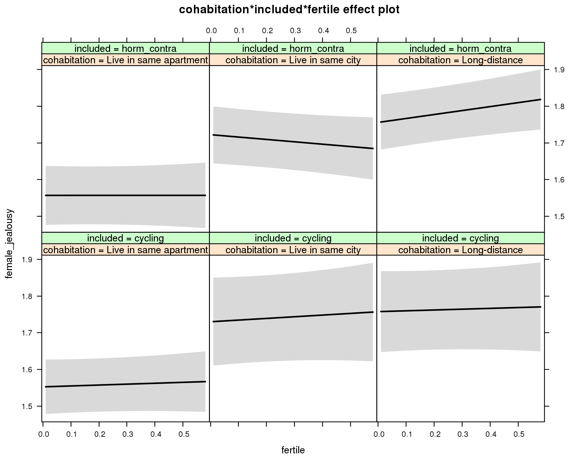
Linear mixed model fit by REML ['lmerMod']
Formula: female_jealousy ~ menstruation + fertile_mean + (1 | person) +
cohabitation + included + fertile + menstruation:included +
cohabitation:included + cohabitation:fertile + included:fertile + cohabitation:included:fertile
Data: diary
REML criterion at convergence: 54542
Scaled residuals:
Min 1Q Median 3Q Max
-3.605 -0.541 -0.132 0.443 7.303
Random effects:
Groups Name Variance Std.Dev.
person (Intercept) 0.282 0.531
Residual 0.406 0.637
Number of obs: 26682, groups: person, 1054
Fixed effects:
Estimate Std. Error t value
(Intercept) 1.566001 0.052838 29.64
menstruationpre 0.007529 0.019443 0.39
menstruationyes 0.009730 0.018324 0.53
fertile_mean -0.095123 0.212057 -0.45
cohabitationLive in same city 0.177354 0.071896 2.47
cohabitationLong-distance 0.204962 0.067738 3.03
includedhorm_contra 0.000319 0.056822 0.01
fertile 0.024593 0.049054 0.50
menstruationpre:includedhorm_contra 0.014044 0.024964 0.56
menstruationyes:includedhorm_contra 0.010067 0.024020 0.42
cohabitationLive in same city:includedhorm_contra -0.011968 0.091869 -0.13
cohabitationLong-distance:includedhorm_contra -0.006211 0.087906 -0.07
cohabitationLive in same city:fertile 0.020878 0.089636 0.23
cohabitationLong-distance:fertile -0.002404 0.080727 -0.03
includedhorm_contra:fertile -0.024483 0.071670 -0.34
cohabitationLive in same city:includedhorm_contra:fertile -0.085842 0.112070 -0.77
cohabitationLong-distance:includedhorm_contra:fertile 0.110062 0.103983 1.06
M_m10: Moderation by relationship status
model %>%
test_moderator("relationship_status_clean", diary)refitting model(s) with ML (instead of REML)
| Df | AIC | BIC | logLik | deviance | Chisq | Chi Df | Pr(>Chisq) | |
|---|---|---|---|---|---|---|---|---|
| with_main | 15 | 54494 | 54617 | -27232 | 54464 | NA | NA | NA |
| with_mod | 19 | 54499 | 54655 | -27231 | 54461 | 3.115 | 4 | 0.5388 |
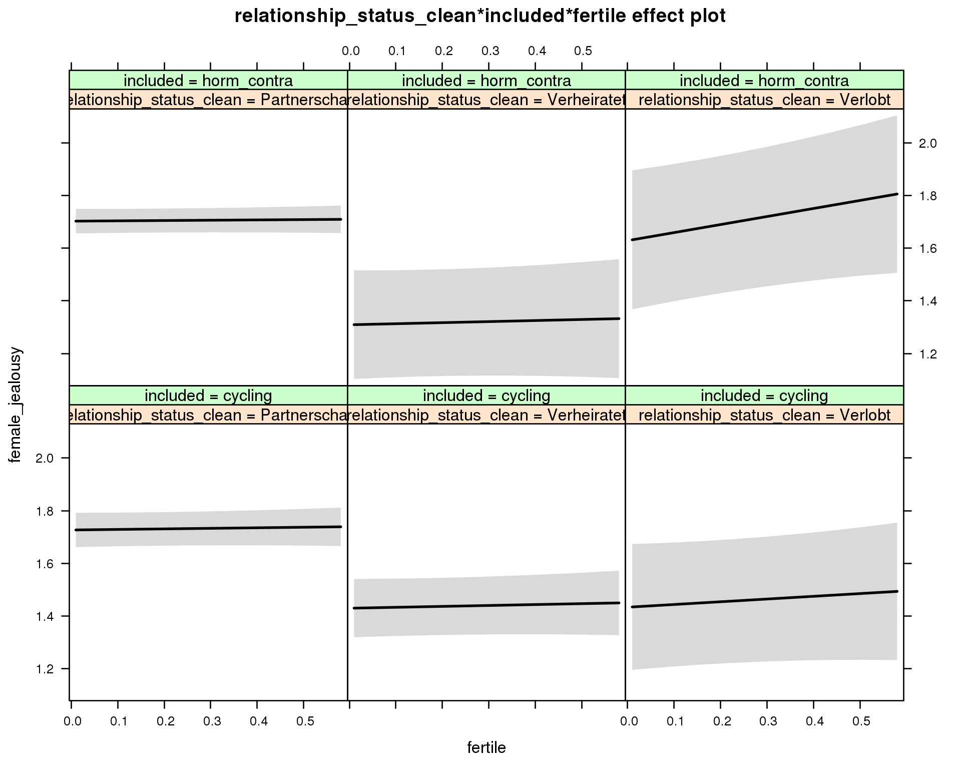
Linear mixed model fit by REML ['lmerMod']
Formula: female_jealousy ~ menstruation + fertile_mean + (1 | person) +
relationship_status_clean + included + fertile + menstruation:included +
relationship_status_clean:included + relationship_status_clean:fertile +
included:fertile + relationship_status_clean:included:fertile
Data: diary
REML criterion at convergence: 54530
Scaled residuals:
Min 1Q Median 3Q Max
-3.614 -0.542 -0.131 0.444 7.290
Random effects:
Groups Name Variance Std.Dev.
person (Intercept) 0.280 0.529
Residual 0.406 0.637
Number of obs: 26682, groups: person, 1054
Fixed effects:
Estimate Std. Error t value
(Intercept) 1.74419 0.04929 35.4
menstruationpre 0.00785 0.01944 0.4
menstruationyes 0.01008 0.01832 0.5
fertile_mean -0.11772 0.21125 -0.6
relationship_status_cleanVerheiratet -0.29690 0.06545 -4.5
relationship_status_cleanVerlobt -0.29314 0.12639 -2.3
includedhorm_contra -0.02860 0.04227 -0.7
fertile 0.02085 0.04493 0.5
menstruationpre:includedhorm_contra 0.01377 0.02496 0.6
menstruationyes:includedhorm_contra 0.01067 0.02402 0.4
relationship_status_cleanVerheiratet:includedhorm_contra -0.09637 0.12620 -0.8
relationship_status_cleanVerlobt:includedhorm_contra 0.21925 0.18642 1.2
relationship_status_cleanVerheiratet:fertile 0.01384 0.07910 0.2
relationship_status_cleanVerlobt:fertile 0.08274 0.14835 0.6
includedhorm_contra:fertile -0.00906 0.05477 -0.2
relationship_status_cleanVerheiratet:includedhorm_contra:fertile 0.01455 0.14896 0.1
relationship_status_cleanVerlobt:includedhorm_contra:fertile 0.21043 0.23039 0.9
Relationship satisfaction
model_summaries$relationship_satisfaction_1Model summary
Model summary
model %>%
print_summary()Linear mixed model fit by REML
t-tests use Satterthwaite approximations to degrees of freedom ['lmerMod']
Formula: relationship_satisfaction_1 ~ included * (menstruation + fertile) + fertile_mean + (1 | person)
Data: diary
REML criterion at convergence: 75048
Scaled residuals:
Min 1Q Median 3Q Max
-4.873 -0.496 0.152 0.648 3.836
Random effects:
Groups Name Variance Std.Dev.
person (Intercept) 0.635 0.797
Residual 0.872 0.934
Number of obs: 26704, groups: person, 1054
Fixed effects:
Estimate Std. Error df t value Pr(>|t|)
(Intercept) 4.7704 0.0690 1328.0000 69.16 <2e-16 ***
includedhorm_contra 0.1788 0.0565 1285.0000 3.16 0.0016 **
menstruationpre 0.0219 0.0285 25963.0000 0.77 0.4434
menstruationyes 0.0240 0.0269 26073.0000 0.89 0.3713
fertile 0.0324 0.0575 25950.0000 0.56 0.5729
fertile_mean -0.4674 0.3159 1442.0000 -1.48 0.1392
includedhorm_contra:menstruationpre -0.0372 0.0366 25960.0000 -1.02 0.3087
includedhorm_contra:menstruationyes -0.0048 0.0352 26050.0000 -0.14 0.8915
includedhorm_contra:fertile -0.1231 0.0729 26076.0000 -1.69 0.0913 .
---
Signif. codes: 0 '***' 0.001 '**' 0.01 '*' 0.05 '.' 0.1 ' ' 1
Correlation of Fixed Effects:
(Intr) incld_ mnstrtnp mnstrtny fertil frtl_m inclddhrm_cntr:mnstrtnp
inclddhrm_c -0.473
menstrutnpr -0.159 0.201
menstrutnys -0.155 0.194 0.397
fertile -0.152 0.249 0.467 0.385
fertile_men -0.772 -0.025 -0.008 -0.005 -0.065
inclddhrm_cntr:mnstrtnp 0.131 -0.252 -0.779 -0.309 -0.363 -0.004
inclddhrm_cntr:mnstrtny 0.124 -0.239 -0.303 -0.763 -0.293 -0.004 0.383
inclddhrm_cntr:f 0.152 -0.315 -0.368 -0.303 -0.787 0.010 0.467
inclddhrm_cntr:mnstrtny
inclddhrm_c
menstrutnpr
menstrutnys
fertile
fertile_men
inclddhrm_cntr:mnstrtnp
inclddhrm_cntr:mnstrtny
inclddhrm_cntr:f 0.381
Effect size standardised by residual variance (\(\frac{b}{ SD_{residual} }\)): 0.03 [-0.09;0.16].
Marginal effect plots
model %>%
plot_all_effects()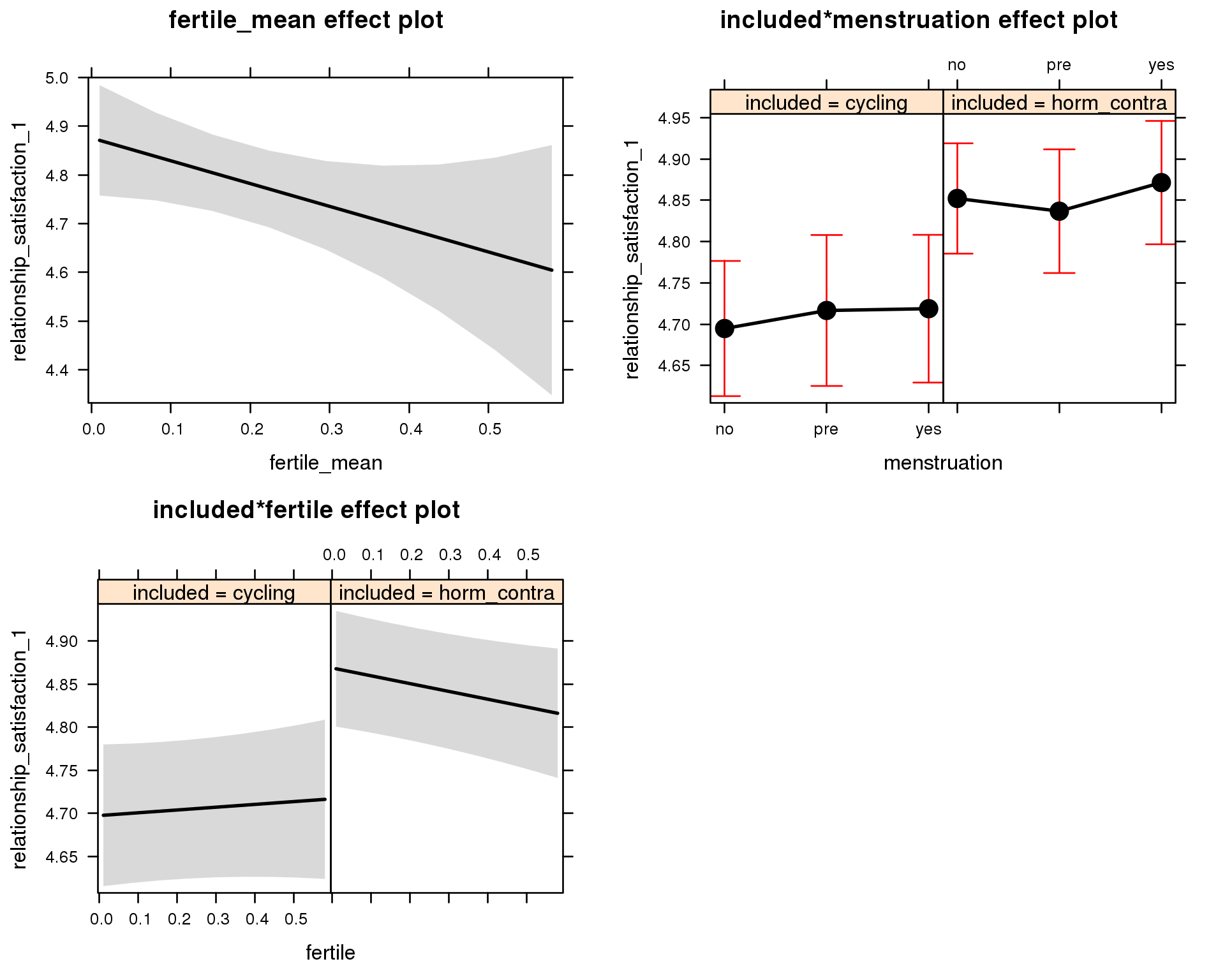
Outcome distribution
model %>%
plot_outcome(diary) + xlab(outcome_label)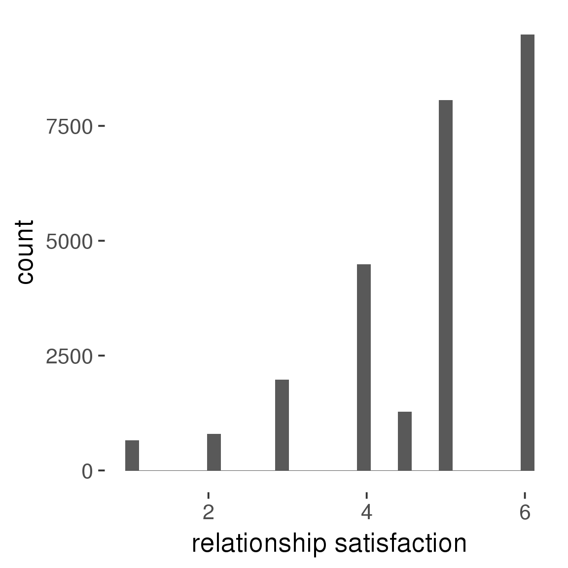
Diagnostics
model %>%
print_diagnostics()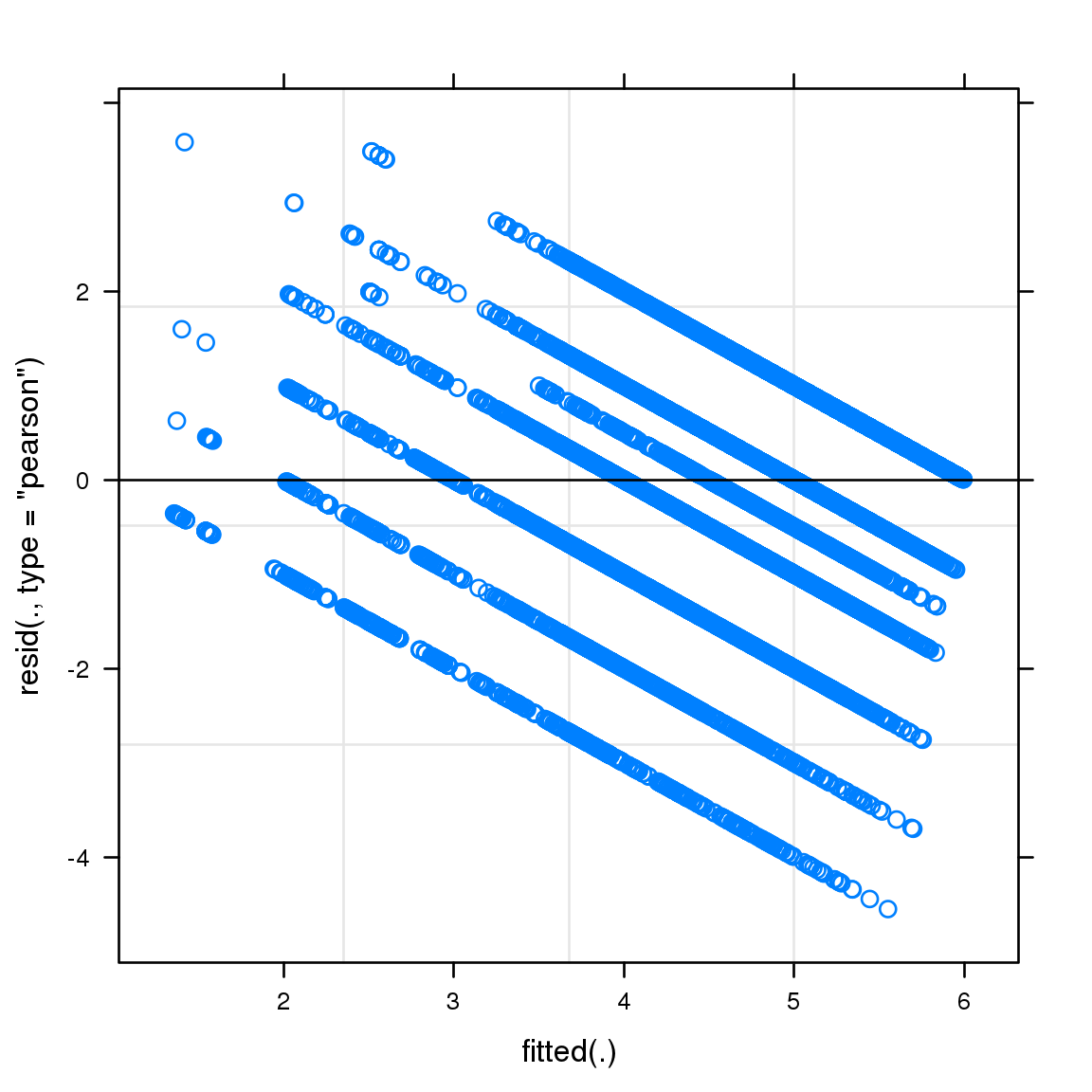
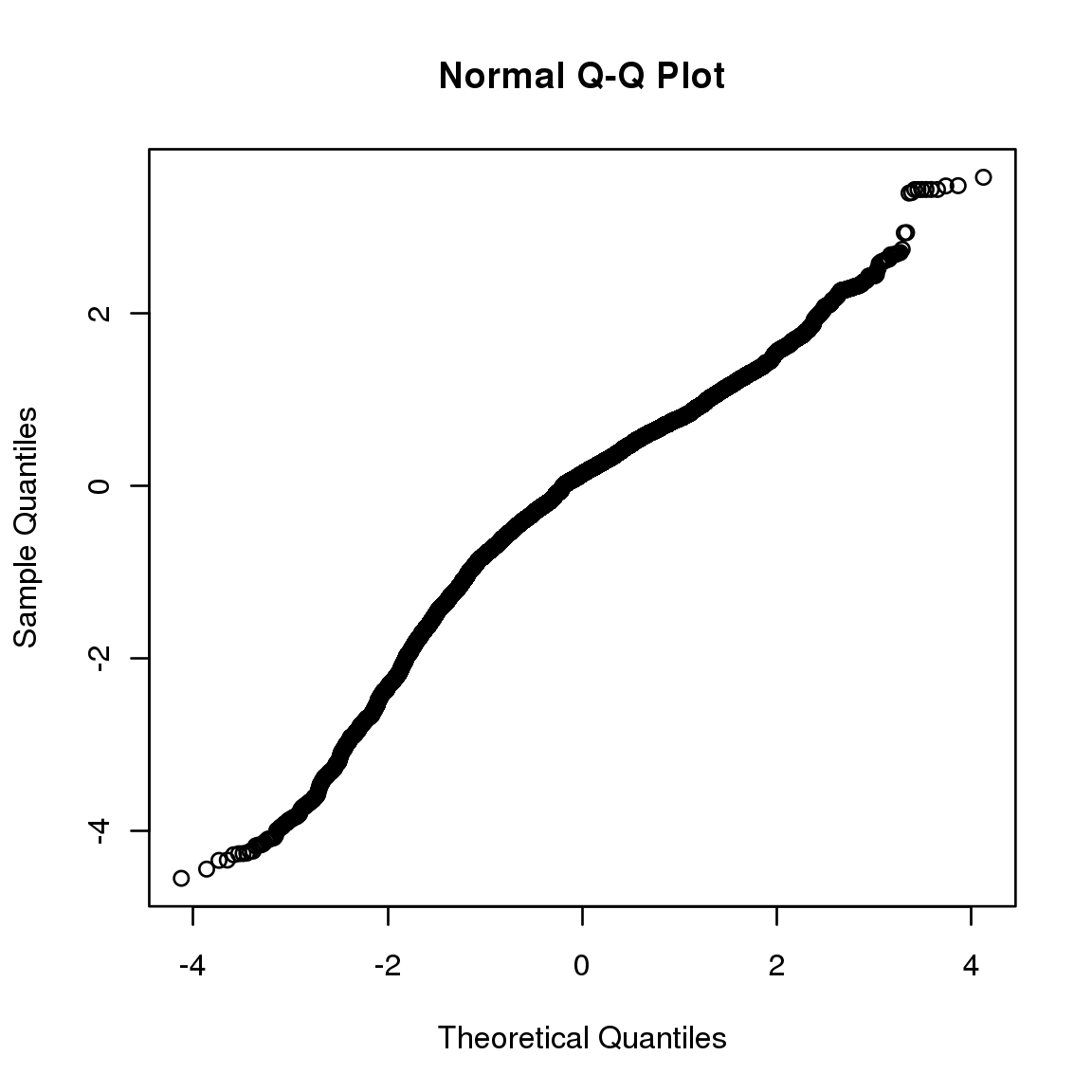

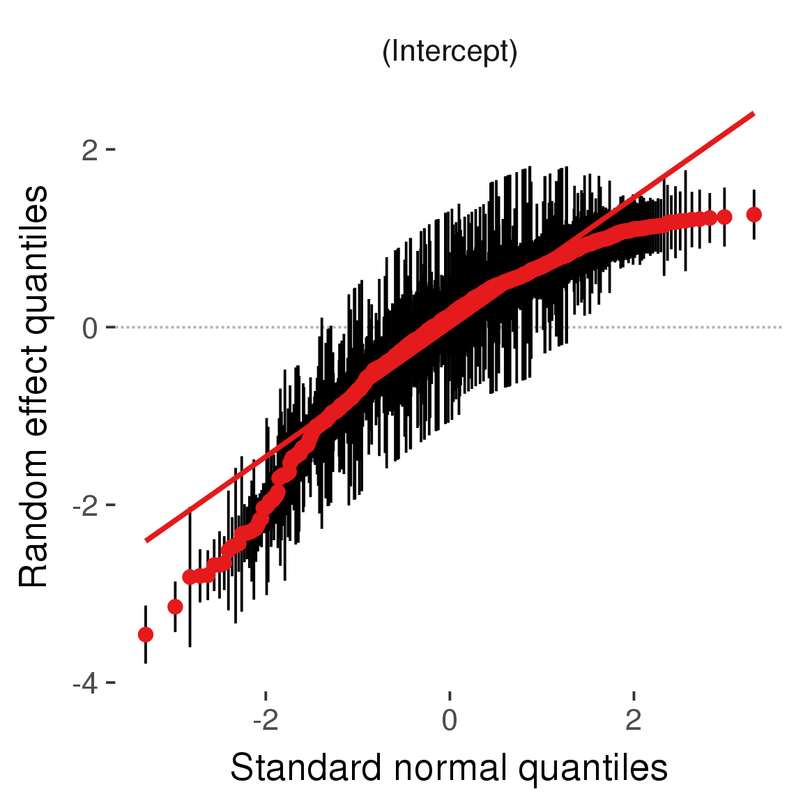
Curves
Here, we continuously plot the outcome over the course of the cycle. Because cycle lengths vary, we subset the data to cycles in a certain range. If the red curve traces the pink curve, our predictor accurately maps the relationship between fertile window probability and the outcome.
Cycle lengths from 21 to 36
Backward-counted
model %>%
plot_curve(diary %>% filter(minimum_cycle_length_diary <= 36, minimum_cycle_length_diary > 20) %>% mutate(fertile=prc_stirn_b))outcome = names(model@frame)[1]
outcome_label = recode(str_replace_all(str_replace_all(str_replace_all(outcome, "_", " "), " pair", "-pair"), " 1", ""),
"desirability 1" = "self-perceived desirability",
"NARQ admiration" = "narcissistic admiration",
"NARQ rivalry" = "narcissistic rivalry",
"extra-pair" = "extra-pair desire & behaviour",
"had sexual intercourse" = "sexual intercourse")
library(ggplot2)
# form a subset and run the model without the hormonal contraception and the fertility predictors
tmp = diary %>%
filter(!is.na(fertile), !is.na(included),
RCD > -1 * minimum_cycle_length_diary, RCD > -40)
new_form = update.formula(formula(model), new = . ~ . - fertile * included)
tmp$residuals = residuals(update(model, new_form, data = tmp , na.action = na.exclude))
tmp = tmp %>%
filter(!is.na(RCD), !is.na(residuals))
rcd_min = min(tmp$RCD)
tmp$real = FALSE
tmp_before = tmp
tmp_before$RCD = tmp_before$RCD + min(tmp$RCD) - 1
tmp_after = tmp
tmp_after$RCD = tmp_after$RCD - min(tmp$RCD) + 1
tmp$real = TRUE
tmp = bind_rows(tmp_before %>% filter(RCD > rcd_min - 11), tmp, tmp_after %>% filter(RCD < 11))GAM smooth on residuals
Here, we partialled out menstruation and individual random effects, then superimposed estimated probability of being in the fertile window scaled to the range of the estimated means. To address the periodicity of the cycle, we prepended and appended ten days of the timeseries to the end and the beginning of the timeseries. We then estimated the GAM and cut off the appended subsets before plotting.
tryCatch({
trend_plot = ggplot(tmp,aes(x = RCD, y = residuals, colour = included)) +
stat_smooth(geom = 'smooth',size = 0.8, fill = "#9ECAE1", method = 'gam', formula = y ~ s(x))
}, error = function(e){cat_message(e, "danger")})
tryCatch({
trend_data = ggplot_build(trend_plot)$data[[1]]
}, error = function(e){cat_message(e, "danger")})
trend_data$RCD = round(trend_data$x)
trend_data = left_join(trend_data, tmp %>% select(real, RCD,fertile) %>% unique(), by = "RCD")
trend_data %>%
filter(real == TRUE) %>%
mutate(superimposed = ( ( (fertile - 0.01)/0.58) * (max(y)-min(y) ) ) + min(y) ) ->
trend_data
ggplot(trend_data) +
geom_ribbon(aes(x = x, ymin = ymin, ymax = ymax, fill = factor(group)), alpha = 0.2) +
geom_line(aes(x = x, y = y, colour = factor(group)), size = 0.8, stat = "identity") +
scale_x_continuous(caption_x) +
geom_line(aes(x = x, y = superimposed), color = "#a83fbf", size = 1, linetype = 'dashed') +
annotate("text",x = mean(trend_data$x), y = max(trend_data$superimposed,na.rm=T) + 0.1, label = 'superimposed fertility peak', color = "#a83fbf") +
scale_y_continuous(outcome_label) +
ggtitle("GAM smooth, residuals") +
scale_color_manual("Contraception status",values = c("2"="black","1"= "red"), labels = c("2"="hormonally\ncontracepting","1"="cycling"), guide = F) +
scale_fill_manual("Contraception status",values = c("2"="black","1"= "red"), labels = c("2"="hormonally\ncontracepting","1"="cycling"), guide = F)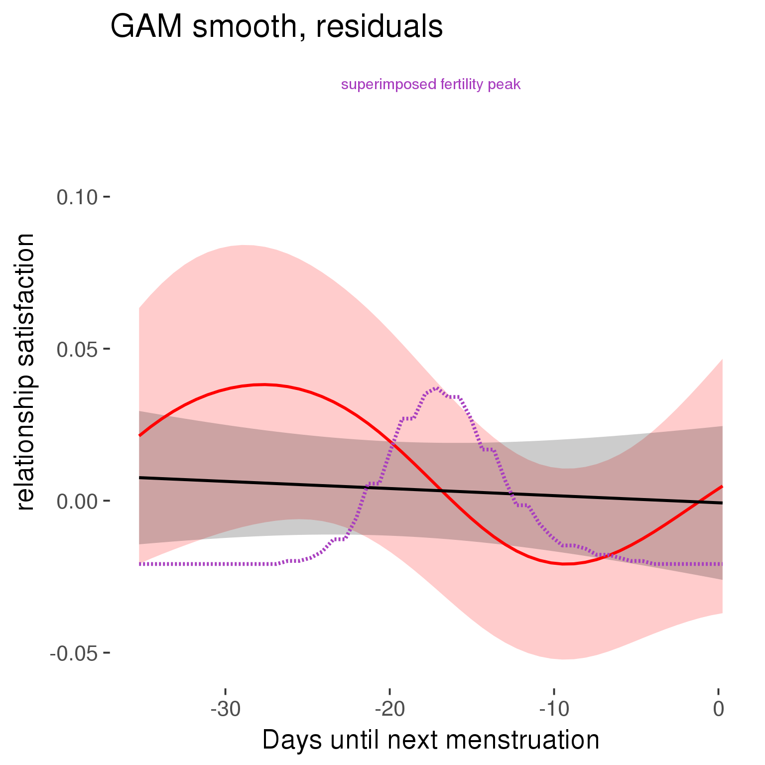
GAM smooth on raw data
As before, but without partialling anything out.
tryCatch({
trend_plot = ggplot(tmp,aes_string(x = "RCD", y = outcome, colour = "included")) +
stat_smooth(geom = 'smooth',size = 0.8, fill = "#9ECAE1", method = 'gam', formula = y ~ s(x))
}, error = function(e){cat_message(e, "danger")})
tryCatch({
trend_data = ggplot_build(trend_plot)$data[[1]]
}, error = function(e){cat_message(e, "danger")})
trend_data$RCD = round(trend_data$x)
trend_data = left_join(trend_data, tmp %>% select(real, RCD,fertile) %>% unique(), by = "RCD")
trend_data %>%
filter(real == TRUE) %>%
mutate(superimposed = ( ( (fertile - 0.01)/0.58) * (max(y)-min(y) ) ) + min(y) ) ->
trend_data
plot1b = ggplot(trend_data) +
geom_ribbon(aes(x = x, ymin = ymin, ymax = ymax, fill = factor(group)), alpha = 0.2) +
geom_line(aes(x = x, y = y, colour = factor(group)), size = 0.8, stat = "identity") +
scale_x_continuous(caption_x) +
geom_line(aes(x = x, y = superimposed), color = "#a83fbf", size = 1, linetype = 'dashed') +
annotate("text",x = mean(trend_data$x), y = max(trend_data$superimposed,na.rm=T) + 0.1, label = 'superimposed fertility peak', color = "#a83fbf") +
scale_y_continuous(outcome_label) +
ggtitle("GAM smooth, raw data") +
scale_color_manual("Contraception status",values = c("2"="black","1"= "red"), labels = c("2"="hormonally\ncontracepting","1"="cycling"), guide = F) +
scale_fill_manual("Contraception status",values = c("2"="black","1"= "red"), labels = c("2"="hormonally\ncontracepting","1"="cycling"), guide = F)
suppressWarnings(print(plot1b))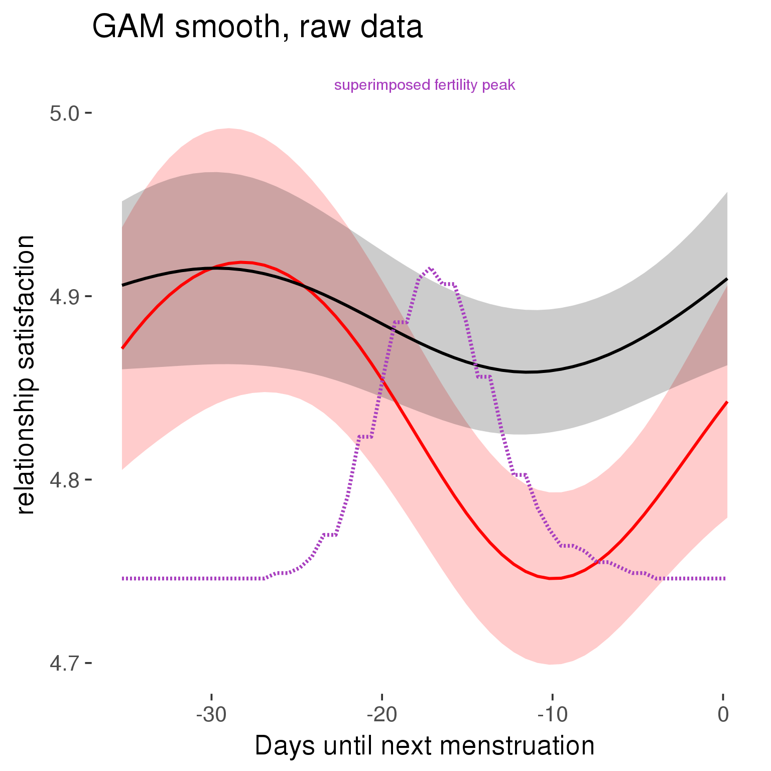
Means and standard errors over raw data
Nothing partialled out, just straight means with bootstrapped confidence intervals.
tryCatch({
trend_plot = ggplot(tmp,aes_string(x = "RCD", y = outcome, colour = "included")) +
geom_pointrange(size = 0.8, stat = 'summary', fun.data = "mean_cl_boot")
}, error = function(e){cat_message(e, "danger")})
tryCatch({
trend_data = ggplot_build(trend_plot)$data[[1]]
}, error = function(e){cat_message(e, "danger")})
trend_data$RCD = round(trend_data$x)
trend_data = left_join(trend_data, tmp %>% select(real, RCD,fertile) %>% unique(), by = "RCD")
trend_data %>%
filter(real == TRUE) %>%
mutate(superimposed = ( ( (fertile - 0.01)/0.58) * (max(y)-min(y) ) ) + min(y) ) ->
trend_data
plot3 = ggplot(trend_data) +
geom_pointrange(aes(x = x, y = y, ymin = ymin,ymax = ymax, colour = factor(group)), size = 0.8, stat = "identity", alpha = 0.6, position = position_dodge(width = .5)) +
scale_x_continuous("Days until next menstruation") +
geom_line(aes(x= x, y = superimposed), color = "#a83fbf", size = 1, linetype = 'dashed') +
annotate("text",x = mean(trend_data$x), y = max(trend_data$superimposed,na.rm=T) + 0.1, label = 'superimposed fertility peak', color = "#a83fbf") +
scale_y_continuous(outcome_label) +
ggtitle("Means with standard errors, raw data") +
scale_color_manual("Contraception status",values = c("2"="black","1"= "red"), labels = c("2"="hormonally\ncontracepting","1"="cycling"), guide = F) +
scale_fill_manual("Contraception status",values = c("2"="black","1"= "red"), labels = c("2"="hormonally\ncontracepting","1"="cycling"), guide = F)
suppressWarnings(print(plot3))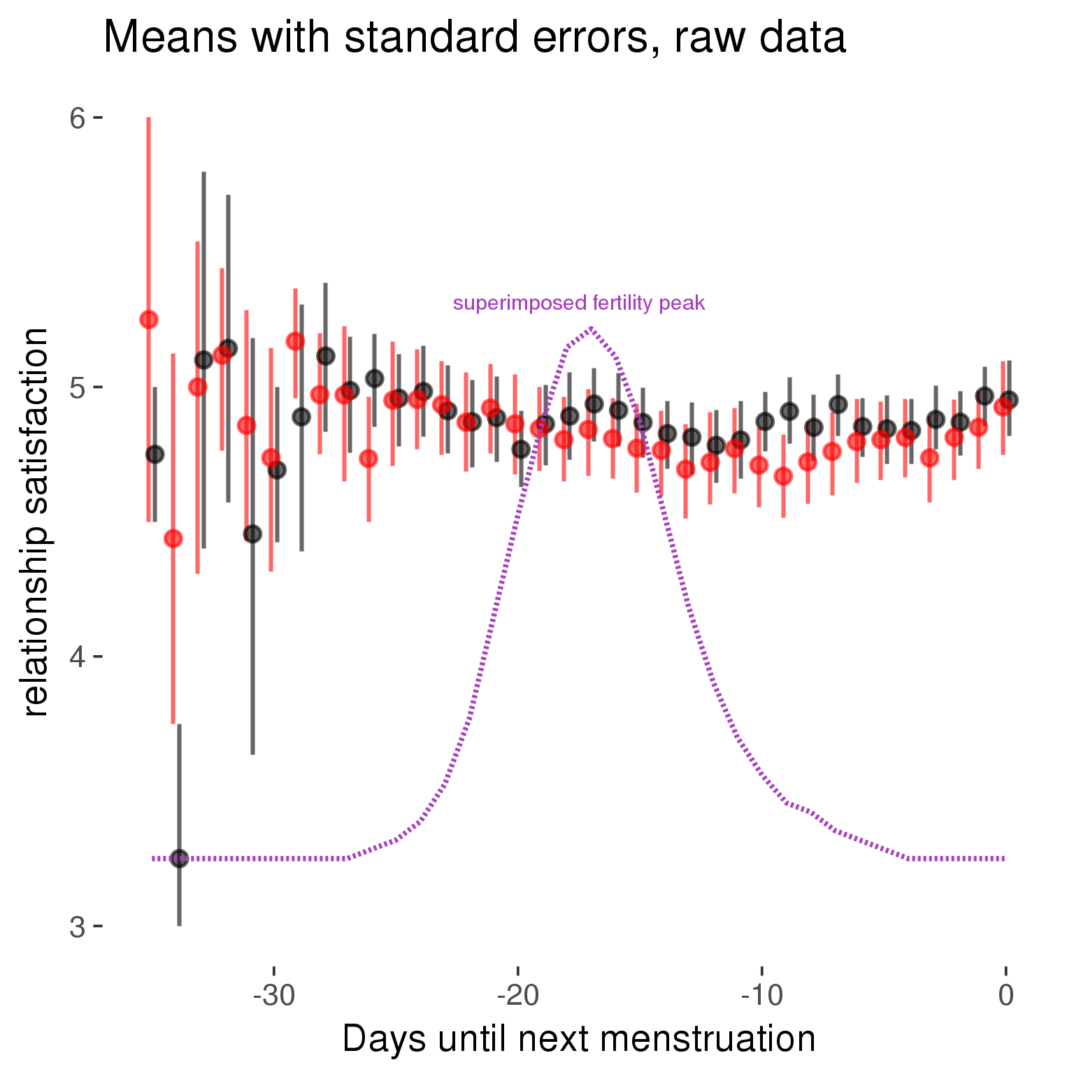
Forward-counted
model %>%
plot_curve(diary %>% filter(minimum_cycle_length_diary <= 36, minimum_cycle_length_diary > 20) %>% mutate(RCD = FCD, fertile = prc_stirn_b_forward_counted), caption_x = "Days since last menstruation")outcome = names(model@frame)[1]
outcome_label = recode(str_replace_all(str_replace_all(str_replace_all(outcome, "_", " "), " pair", "-pair"), " 1", ""),
"desirability 1" = "self-perceived desirability",
"NARQ admiration" = "narcissistic admiration",
"NARQ rivalry" = "narcissistic rivalry",
"extra-pair" = "extra-pair desire & behaviour",
"had sexual intercourse" = "sexual intercourse")
library(ggplot2)
# form a subset and run the model without the hormonal contraception and the fertility predictors
tmp = diary %>%
filter(!is.na(fertile), !is.na(included),
RCD > -1 * minimum_cycle_length_diary, RCD > -40)
new_form = update.formula(formula(model), new = . ~ . - fertile * included)
tmp$residuals = residuals(update(model, new_form, data = tmp , na.action = na.exclude))
tmp = tmp %>%
filter(!is.na(RCD), !is.na(residuals))
rcd_min = min(tmp$RCD)
tmp$real = FALSE
tmp_before = tmp
tmp_before$RCD = tmp_before$RCD + min(tmp$RCD) - 1
tmp_after = tmp
tmp_after$RCD = tmp_after$RCD - min(tmp$RCD) + 1
tmp$real = TRUE
tmp = bind_rows(tmp_before %>% filter(RCD > rcd_min - 11), tmp, tmp_after %>% filter(RCD < 11))GAM smooth on residuals
Here, we partialled out menstruation and individual random effects, then superimposed estimated probability of being in the fertile window scaled to the range of the estimated means. To address the periodicity of the cycle, we prepended and appended ten days of the timeseries to the end and the beginning of the timeseries. We then estimated the GAM and cut off the appended subsets before plotting.
tryCatch({
trend_plot = ggplot(tmp,aes(x = RCD, y = residuals, colour = included)) +
stat_smooth(geom = 'smooth',size = 0.8, fill = "#9ECAE1", method = 'gam', formula = y ~ s(x))
}, error = function(e){cat_message(e, "danger")})
tryCatch({
trend_data = ggplot_build(trend_plot)$data[[1]]
}, error = function(e){cat_message(e, "danger")})
trend_data$RCD = round(trend_data$x)
trend_data = left_join(trend_data, tmp %>% select(real, RCD,fertile) %>% unique(), by = "RCD")
trend_data %>%
filter(real == TRUE) %>%
mutate(superimposed = ( ( (fertile - 0.01)/0.58) * (max(y)-min(y) ) ) + min(y) ) ->
trend_data
ggplot(trend_data) +
geom_ribbon(aes(x = x, ymin = ymin, ymax = ymax, fill = factor(group)), alpha = 0.2) +
geom_line(aes(x = x, y = y, colour = factor(group)), size = 0.8, stat = "identity") +
scale_x_continuous(caption_x) +
geom_line(aes(x = x, y = superimposed), color = "#a83fbf", size = 1, linetype = 'dashed') +
annotate("text",x = mean(trend_data$x), y = max(trend_data$superimposed,na.rm=T) + 0.1, label = 'superimposed fertility peak', color = "#a83fbf") +
scale_y_continuous(outcome_label) +
ggtitle("GAM smooth, residuals") +
scale_color_manual("Contraception status",values = c("2"="black","1"= "red"), labels = c("2"="hormonally\ncontracepting","1"="cycling"), guide = F) +
scale_fill_manual("Contraception status",values = c("2"="black","1"= "red"), labels = c("2"="hormonally\ncontracepting","1"="cycling"), guide = F)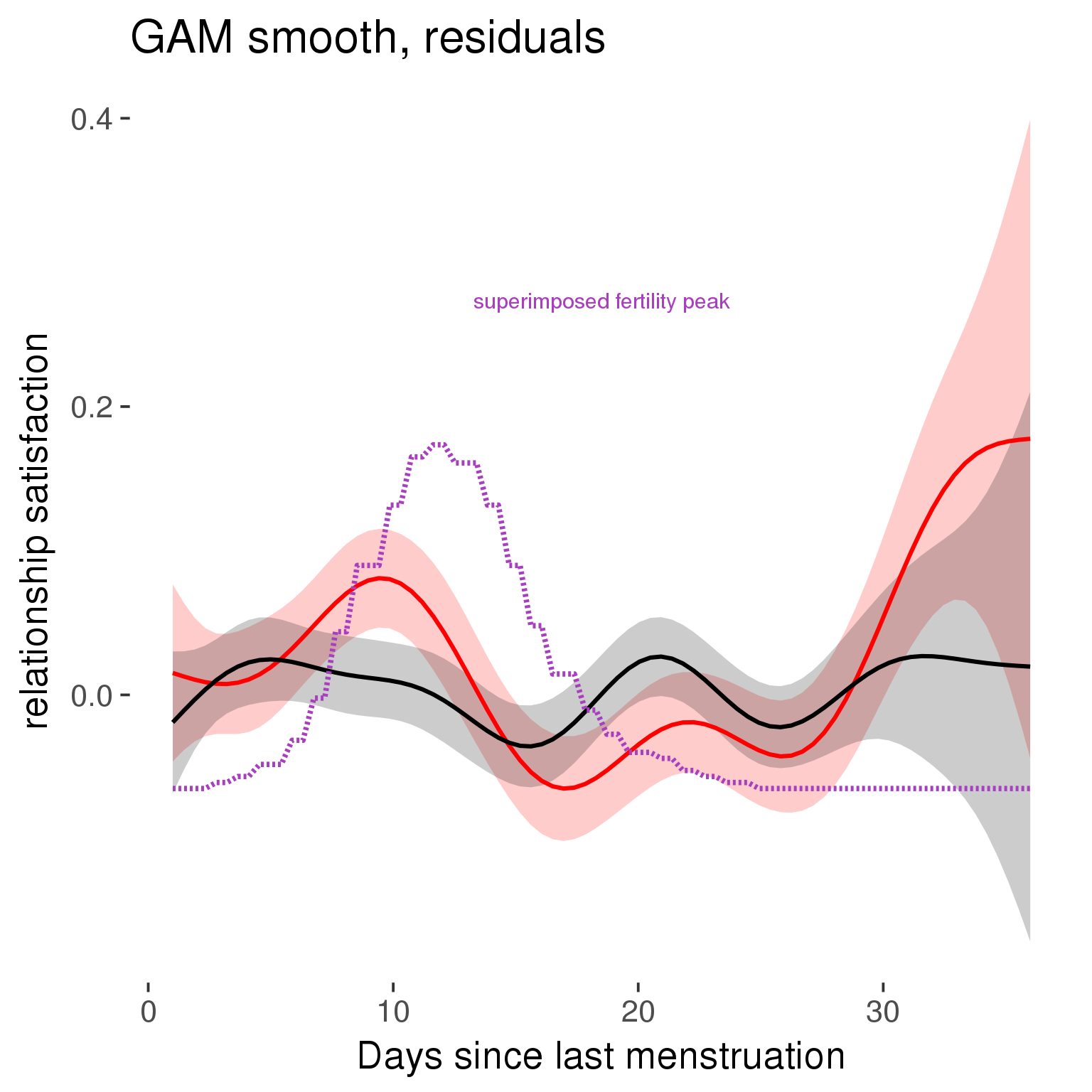
GAM smooth on raw data
As before, but without partialling anything out.
tryCatch({
trend_plot = ggplot(tmp,aes_string(x = "RCD", y = outcome, colour = "included")) +
stat_smooth(geom = 'smooth',size = 0.8, fill = "#9ECAE1", method = 'gam', formula = y ~ s(x))
}, error = function(e){cat_message(e, "danger")})
tryCatch({
trend_data = ggplot_build(trend_plot)$data[[1]]
}, error = function(e){cat_message(e, "danger")})
trend_data$RCD = round(trend_data$x)
trend_data = left_join(trend_data, tmp %>% select(real, RCD,fertile) %>% unique(), by = "RCD")
trend_data %>%
filter(real == TRUE) %>%
mutate(superimposed = ( ( (fertile - 0.01)/0.58) * (max(y)-min(y) ) ) + min(y) ) ->
trend_data
plot1b = ggplot(trend_data) +
geom_ribbon(aes(x = x, ymin = ymin, ymax = ymax, fill = factor(group)), alpha = 0.2) +
geom_line(aes(x = x, y = y, colour = factor(group)), size = 0.8, stat = "identity") +
scale_x_continuous(caption_x) +
geom_line(aes(x = x, y = superimposed), color = "#a83fbf", size = 1, linetype = 'dashed') +
annotate("text",x = mean(trend_data$x), y = max(trend_data$superimposed,na.rm=T) + 0.1, label = 'superimposed fertility peak', color = "#a83fbf") +
scale_y_continuous(outcome_label) +
ggtitle("GAM smooth, raw data") +
scale_color_manual("Contraception status",values = c("2"="black","1"= "red"), labels = c("2"="hormonally\ncontracepting","1"="cycling"), guide = F) +
scale_fill_manual("Contraception status",values = c("2"="black","1"= "red"), labels = c("2"="hormonally\ncontracepting","1"="cycling"), guide = F)
suppressWarnings(print(plot1b))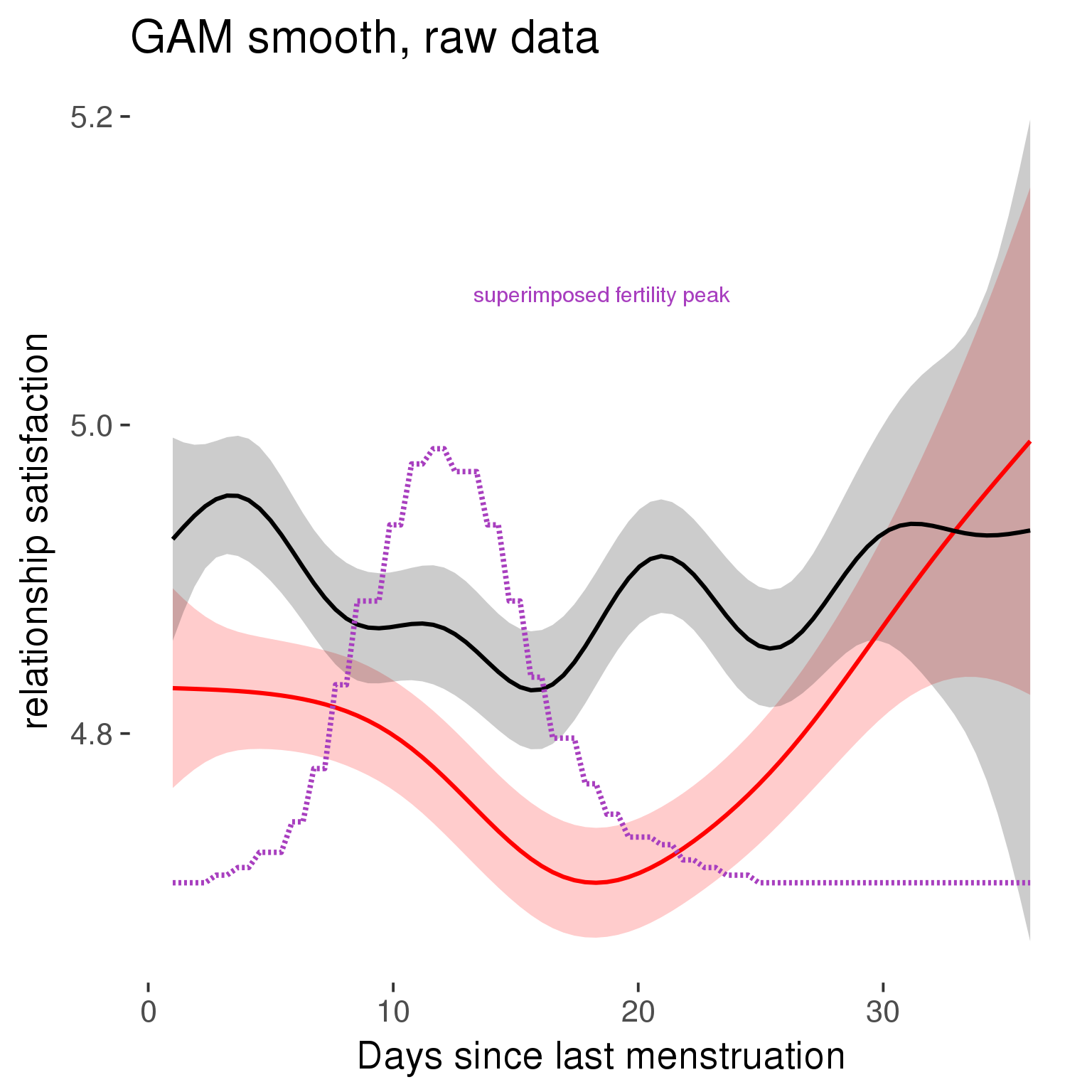
Means and standard errors over raw data
Nothing partialled out, just straight means with bootstrapped confidence intervals.
tryCatch({
trend_plot = ggplot(tmp,aes_string(x = "RCD", y = outcome, colour = "included")) +
geom_pointrange(size = 0.8, stat = 'summary', fun.data = "mean_cl_boot")
}, error = function(e){cat_message(e, "danger")})
tryCatch({
trend_data = ggplot_build(trend_plot)$data[[1]]
}, error = function(e){cat_message(e, "danger")})
trend_data$RCD = round(trend_data$x)
trend_data = left_join(trend_data, tmp %>% select(real, RCD,fertile) %>% unique(), by = "RCD")
trend_data %>%
filter(real == TRUE) %>%
mutate(superimposed = ( ( (fertile - 0.01)/0.58) * (max(y)-min(y) ) ) + min(y) ) ->
trend_data
plot3 = ggplot(trend_data) +
geom_pointrange(aes(x = x, y = y, ymin = ymin,ymax = ymax, colour = factor(group)), size = 0.8, stat = "identity", alpha = 0.6, position = position_dodge(width = .5)) +
scale_x_continuous("Days until next menstruation") +
geom_line(aes(x= x, y = superimposed), color = "#a83fbf", size = 1, linetype = 'dashed') +
annotate("text",x = mean(trend_data$x), y = max(trend_data$superimposed,na.rm=T) + 0.1, label = 'superimposed fertility peak', color = "#a83fbf") +
scale_y_continuous(outcome_label) +
ggtitle("Means with standard errors, raw data") +
scale_color_manual("Contraception status",values = c("2"="black","1"= "red"), labels = c("2"="hormonally\ncontracepting","1"="cycling"), guide = F) +
scale_fill_manual("Contraception status",values = c("2"="black","1"= "red"), labels = c("2"="hormonally\ncontracepting","1"="cycling"), guide = F)
suppressWarnings(print(plot3))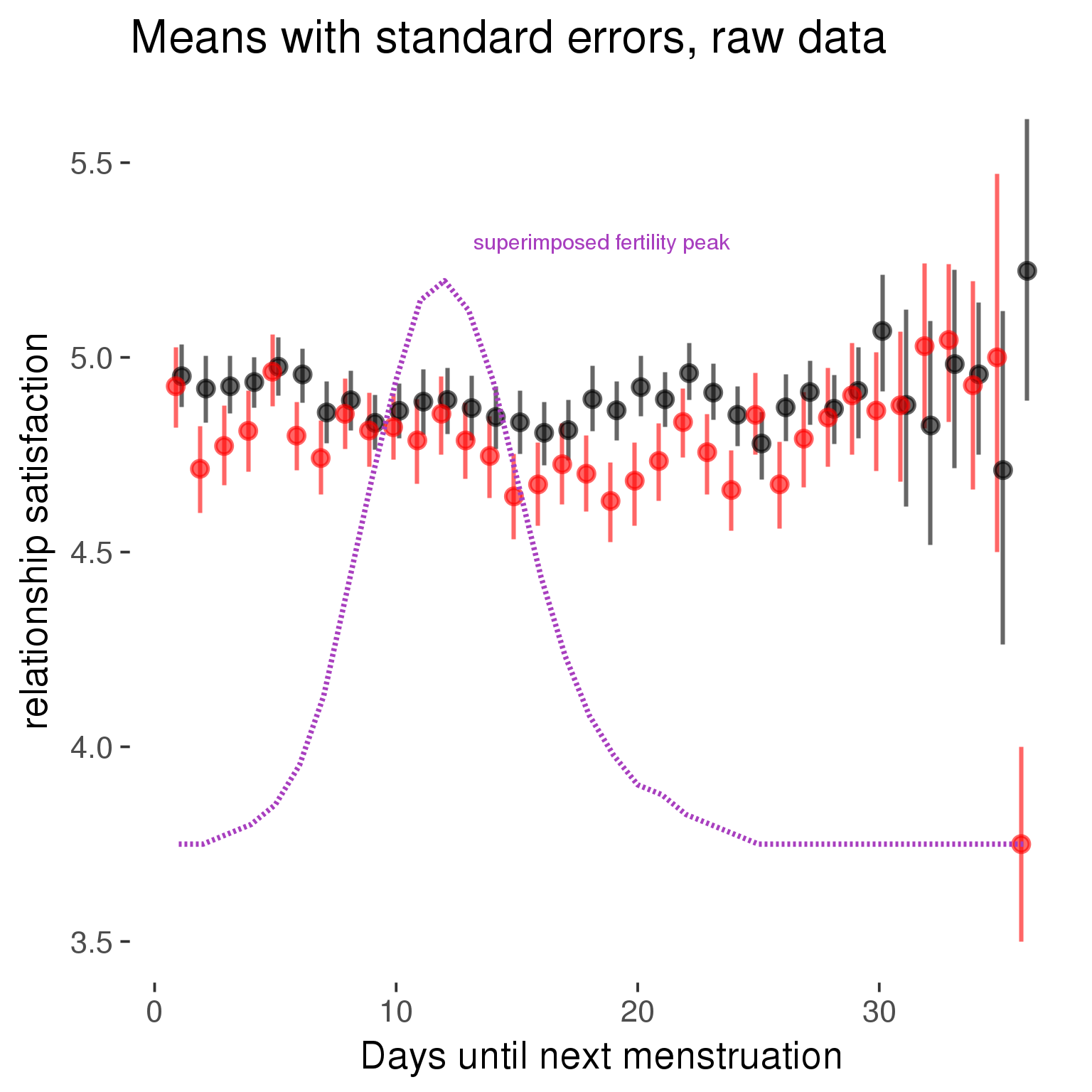
Cycle lengths from 27 to 30
Backward-counted
model %>%
plot_curve(diary %>% filter(minimum_cycle_length_diary <= 30, minimum_cycle_length_diary >= 27) %>% mutate(fertile=prc_stirn_b))outcome = names(model@frame)[1]
outcome_label = recode(str_replace_all(str_replace_all(str_replace_all(outcome, "_", " "), " pair", "-pair"), " 1", ""),
"desirability 1" = "self-perceived desirability",
"NARQ admiration" = "narcissistic admiration",
"NARQ rivalry" = "narcissistic rivalry",
"extra-pair" = "extra-pair desire & behaviour",
"had sexual intercourse" = "sexual intercourse")
library(ggplot2)
# form a subset and run the model without the hormonal contraception and the fertility predictors
tmp = diary %>%
filter(!is.na(fertile), !is.na(included),
RCD > -1 * minimum_cycle_length_diary, RCD > -40)
new_form = update.formula(formula(model), new = . ~ . - fertile * included)
tmp$residuals = residuals(update(model, new_form, data = tmp , na.action = na.exclude))
tmp = tmp %>%
filter(!is.na(RCD), !is.na(residuals))
rcd_min = min(tmp$RCD)
tmp$real = FALSE
tmp_before = tmp
tmp_before$RCD = tmp_before$RCD + min(tmp$RCD) - 1
tmp_after = tmp
tmp_after$RCD = tmp_after$RCD - min(tmp$RCD) + 1
tmp$real = TRUE
tmp = bind_rows(tmp_before %>% filter(RCD > rcd_min - 11), tmp, tmp_after %>% filter(RCD < 11))GAM smooth on residuals
Here, we partialled out menstruation and individual random effects, then superimposed estimated probability of being in the fertile window scaled to the range of the estimated means. To address the periodicity of the cycle, we prepended and appended ten days of the timeseries to the end and the beginning of the timeseries. We then estimated the GAM and cut off the appended subsets before plotting.
tryCatch({
trend_plot = ggplot(tmp,aes(x = RCD, y = residuals, colour = included)) +
stat_smooth(geom = 'smooth',size = 0.8, fill = "#9ECAE1", method = 'gam', formula = y ~ s(x))
}, error = function(e){cat_message(e, "danger")})
tryCatch({
trend_data = ggplot_build(trend_plot)$data[[1]]
}, error = function(e){cat_message(e, "danger")})
trend_data$RCD = round(trend_data$x)
trend_data = left_join(trend_data, tmp %>% select(real, RCD,fertile) %>% unique(), by = "RCD")
trend_data %>%
filter(real == TRUE) %>%
mutate(superimposed = ( ( (fertile - 0.01)/0.58) * (max(y)-min(y) ) ) + min(y) ) ->
trend_data
ggplot(trend_data) +
geom_ribbon(aes(x = x, ymin = ymin, ymax = ymax, fill = factor(group)), alpha = 0.2) +
geom_line(aes(x = x, y = y, colour = factor(group)), size = 0.8, stat = "identity") +
scale_x_continuous(caption_x) +
geom_line(aes(x = x, y = superimposed), color = "#a83fbf", size = 1, linetype = 'dashed') +
annotate("text",x = mean(trend_data$x), y = max(trend_data$superimposed,na.rm=T) + 0.1, label = 'superimposed fertility peak', color = "#a83fbf") +
scale_y_continuous(outcome_label) +
ggtitle("GAM smooth, residuals") +
scale_color_manual("Contraception status",values = c("2"="black","1"= "red"), labels = c("2"="hormonally\ncontracepting","1"="cycling"), guide = F) +
scale_fill_manual("Contraception status",values = c("2"="black","1"= "red"), labels = c("2"="hormonally\ncontracepting","1"="cycling"), guide = F)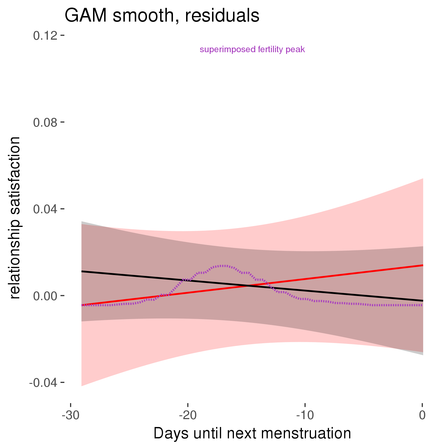
GAM smooth on raw data
As before, but without partialling anything out.
tryCatch({
trend_plot = ggplot(tmp,aes_string(x = "RCD", y = outcome, colour = "included")) +
stat_smooth(geom = 'smooth',size = 0.8, fill = "#9ECAE1", method = 'gam', formula = y ~ s(x))
}, error = function(e){cat_message(e, "danger")})
tryCatch({
trend_data = ggplot_build(trend_plot)$data[[1]]
}, error = function(e){cat_message(e, "danger")})
trend_data$RCD = round(trend_data$x)
trend_data = left_join(trend_data, tmp %>% select(real, RCD,fertile) %>% unique(), by = "RCD")
trend_data %>%
filter(real == TRUE) %>%
mutate(superimposed = ( ( (fertile - 0.01)/0.58) * (max(y)-min(y) ) ) + min(y) ) ->
trend_data
plot1b = ggplot(trend_data) +
geom_ribbon(aes(x = x, ymin = ymin, ymax = ymax, fill = factor(group)), alpha = 0.2) +
geom_line(aes(x = x, y = y, colour = factor(group)), size = 0.8, stat = "identity") +
scale_x_continuous(caption_x) +
geom_line(aes(x = x, y = superimposed), color = "#a83fbf", size = 1, linetype = 'dashed') +
annotate("text",x = mean(trend_data$x), y = max(trend_data$superimposed,na.rm=T) + 0.1, label = 'superimposed fertility peak', color = "#a83fbf") +
scale_y_continuous(outcome_label) +
ggtitle("GAM smooth, raw data") +
scale_color_manual("Contraception status",values = c("2"="black","1"= "red"), labels = c("2"="hormonally\ncontracepting","1"="cycling"), guide = F) +
scale_fill_manual("Contraception status",values = c("2"="black","1"= "red"), labels = c("2"="hormonally\ncontracepting","1"="cycling"), guide = F)
suppressWarnings(print(plot1b))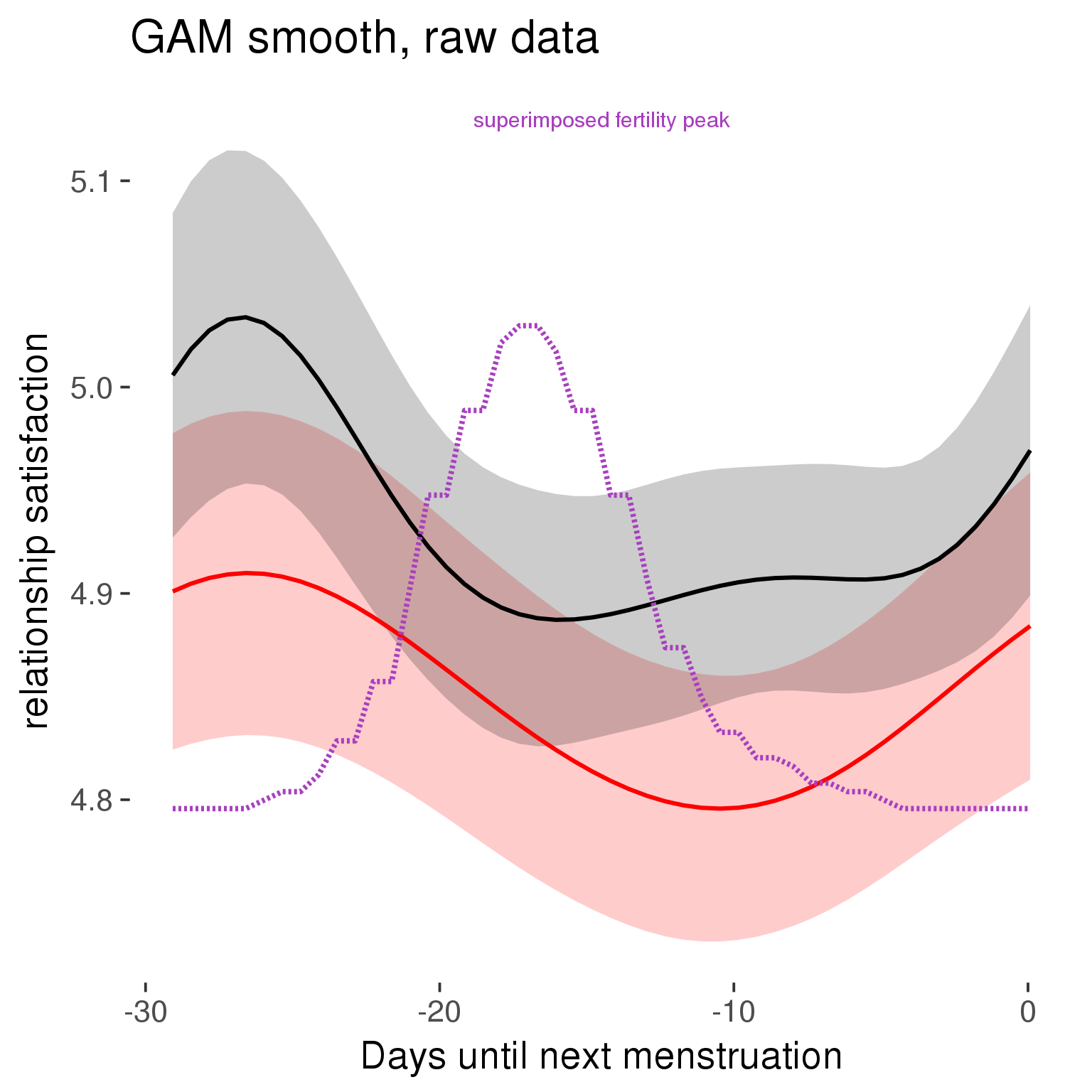
Means and standard errors over raw data
Nothing partialled out, just straight means with bootstrapped confidence intervals.
tryCatch({
trend_plot = ggplot(tmp,aes_string(x = "RCD", y = outcome, colour = "included")) +
geom_pointrange(size = 0.8, stat = 'summary', fun.data = "mean_cl_boot")
}, error = function(e){cat_message(e, "danger")})
tryCatch({
trend_data = ggplot_build(trend_plot)$data[[1]]
}, error = function(e){cat_message(e, "danger")})
trend_data$RCD = round(trend_data$x)
trend_data = left_join(trend_data, tmp %>% select(real, RCD,fertile) %>% unique(), by = "RCD")
trend_data %>%
filter(real == TRUE) %>%
mutate(superimposed = ( ( (fertile - 0.01)/0.58) * (max(y)-min(y) ) ) + min(y) ) ->
trend_data
plot3 = ggplot(trend_data) +
geom_pointrange(aes(x = x, y = y, ymin = ymin,ymax = ymax, colour = factor(group)), size = 0.8, stat = "identity", alpha = 0.6, position = position_dodge(width = .5)) +
scale_x_continuous("Days until next menstruation") +
geom_line(aes(x= x, y = superimposed), color = "#a83fbf", size = 1, linetype = 'dashed') +
annotate("text",x = mean(trend_data$x), y = max(trend_data$superimposed,na.rm=T) + 0.1, label = 'superimposed fertility peak', color = "#a83fbf") +
scale_y_continuous(outcome_label) +
ggtitle("Means with standard errors, raw data") +
scale_color_manual("Contraception status",values = c("2"="black","1"= "red"), labels = c("2"="hormonally\ncontracepting","1"="cycling"), guide = F) +
scale_fill_manual("Contraception status",values = c("2"="black","1"= "red"), labels = c("2"="hormonally\ncontracepting","1"="cycling"), guide = F)
suppressWarnings(print(plot3))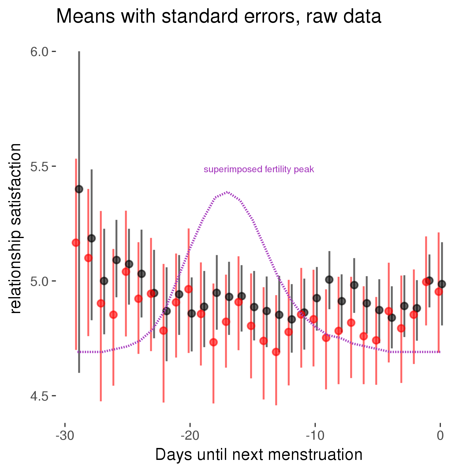
Forward-counted
model %>%
plot_curve(diary %>% filter(minimum_cycle_length_diary <= 30, minimum_cycle_length_diary >= 27) %>% mutate(RCD = FCD, fertile = prc_stirn_b_forward_counted), caption_x = "Days since last menstruation")outcome = names(model@frame)[1]
outcome_label = recode(str_replace_all(str_replace_all(str_replace_all(outcome, "_", " "), " pair", "-pair"), " 1", ""),
"desirability 1" = "self-perceived desirability",
"NARQ admiration" = "narcissistic admiration",
"NARQ rivalry" = "narcissistic rivalry",
"extra-pair" = "extra-pair desire & behaviour",
"had sexual intercourse" = "sexual intercourse")
library(ggplot2)
# form a subset and run the model without the hormonal contraception and the fertility predictors
tmp = diary %>%
filter(!is.na(fertile), !is.na(included),
RCD > -1 * minimum_cycle_length_diary, RCD > -40)
new_form = update.formula(formula(model), new = . ~ . - fertile * included)
tmp$residuals = residuals(update(model, new_form, data = tmp , na.action = na.exclude))
tmp = tmp %>%
filter(!is.na(RCD), !is.na(residuals))
rcd_min = min(tmp$RCD)
tmp$real = FALSE
tmp_before = tmp
tmp_before$RCD = tmp_before$RCD + min(tmp$RCD) - 1
tmp_after = tmp
tmp_after$RCD = tmp_after$RCD - min(tmp$RCD) + 1
tmp$real = TRUE
tmp = bind_rows(tmp_before %>% filter(RCD > rcd_min - 11), tmp, tmp_after %>% filter(RCD < 11))GAM smooth on residuals
Here, we partialled out menstruation and individual random effects, then superimposed estimated probability of being in the fertile window scaled to the range of the estimated means. To address the periodicity of the cycle, we prepended and appended ten days of the timeseries to the end and the beginning of the timeseries. We then estimated the GAM and cut off the appended subsets before plotting.
tryCatch({
trend_plot = ggplot(tmp,aes(x = RCD, y = residuals, colour = included)) +
stat_smooth(geom = 'smooth',size = 0.8, fill = "#9ECAE1", method = 'gam', formula = y ~ s(x))
}, error = function(e){cat_message(e, "danger")})
tryCatch({
trend_data = ggplot_build(trend_plot)$data[[1]]
}, error = function(e){cat_message(e, "danger")})
trend_data$RCD = round(trend_data$x)
trend_data = left_join(trend_data, tmp %>% select(real, RCD,fertile) %>% unique(), by = "RCD")
trend_data %>%
filter(real == TRUE) %>%
mutate(superimposed = ( ( (fertile - 0.01)/0.58) * (max(y)-min(y) ) ) + min(y) ) ->
trend_data
ggplot(trend_data) +
geom_ribbon(aes(x = x, ymin = ymin, ymax = ymax, fill = factor(group)), alpha = 0.2) +
geom_line(aes(x = x, y = y, colour = factor(group)), size = 0.8, stat = "identity") +
scale_x_continuous(caption_x) +
geom_line(aes(x = x, y = superimposed), color = "#a83fbf", size = 1, linetype = 'dashed') +
annotate("text",x = mean(trend_data$x), y = max(trend_data$superimposed,na.rm=T) + 0.1, label = 'superimposed fertility peak', color = "#a83fbf") +
scale_y_continuous(outcome_label) +
ggtitle("GAM smooth, residuals") +
scale_color_manual("Contraception status",values = c("2"="black","1"= "red"), labels = c("2"="hormonally\ncontracepting","1"="cycling"), guide = F) +
scale_fill_manual("Contraception status",values = c("2"="black","1"= "red"), labels = c("2"="hormonally\ncontracepting","1"="cycling"), guide = F)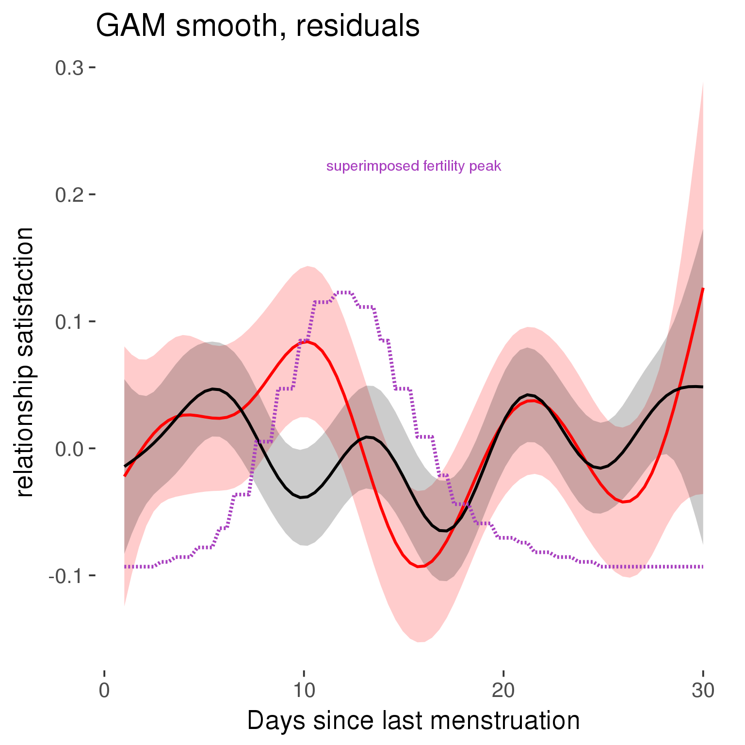
GAM smooth on raw data
As before, but without partialling anything out.
tryCatch({
trend_plot = ggplot(tmp,aes_string(x = "RCD", y = outcome, colour = "included")) +
stat_smooth(geom = 'smooth',size = 0.8, fill = "#9ECAE1", method = 'gam', formula = y ~ s(x))
}, error = function(e){cat_message(e, "danger")})
tryCatch({
trend_data = ggplot_build(trend_plot)$data[[1]]
}, error = function(e){cat_message(e, "danger")})
trend_data$RCD = round(trend_data$x)
trend_data = left_join(trend_data, tmp %>% select(real, RCD,fertile) %>% unique(), by = "RCD")
trend_data %>%
filter(real == TRUE) %>%
mutate(superimposed = ( ( (fertile - 0.01)/0.58) * (max(y)-min(y) ) ) + min(y) ) ->
trend_data
plot1b = ggplot(trend_data) +
geom_ribbon(aes(x = x, ymin = ymin, ymax = ymax, fill = factor(group)), alpha = 0.2) +
geom_line(aes(x = x, y = y, colour = factor(group)), size = 0.8, stat = "identity") +
scale_x_continuous(caption_x) +
geom_line(aes(x = x, y = superimposed), color = "#a83fbf", size = 1, linetype = 'dashed') +
annotate("text",x = mean(trend_data$x), y = max(trend_data$superimposed,na.rm=T) + 0.1, label = 'superimposed fertility peak', color = "#a83fbf") +
scale_y_continuous(outcome_label) +
ggtitle("GAM smooth, raw data") +
scale_color_manual("Contraception status",values = c("2"="black","1"= "red"), labels = c("2"="hormonally\ncontracepting","1"="cycling"), guide = F) +
scale_fill_manual("Contraception status",values = c("2"="black","1"= "red"), labels = c("2"="hormonally\ncontracepting","1"="cycling"), guide = F)
suppressWarnings(print(plot1b))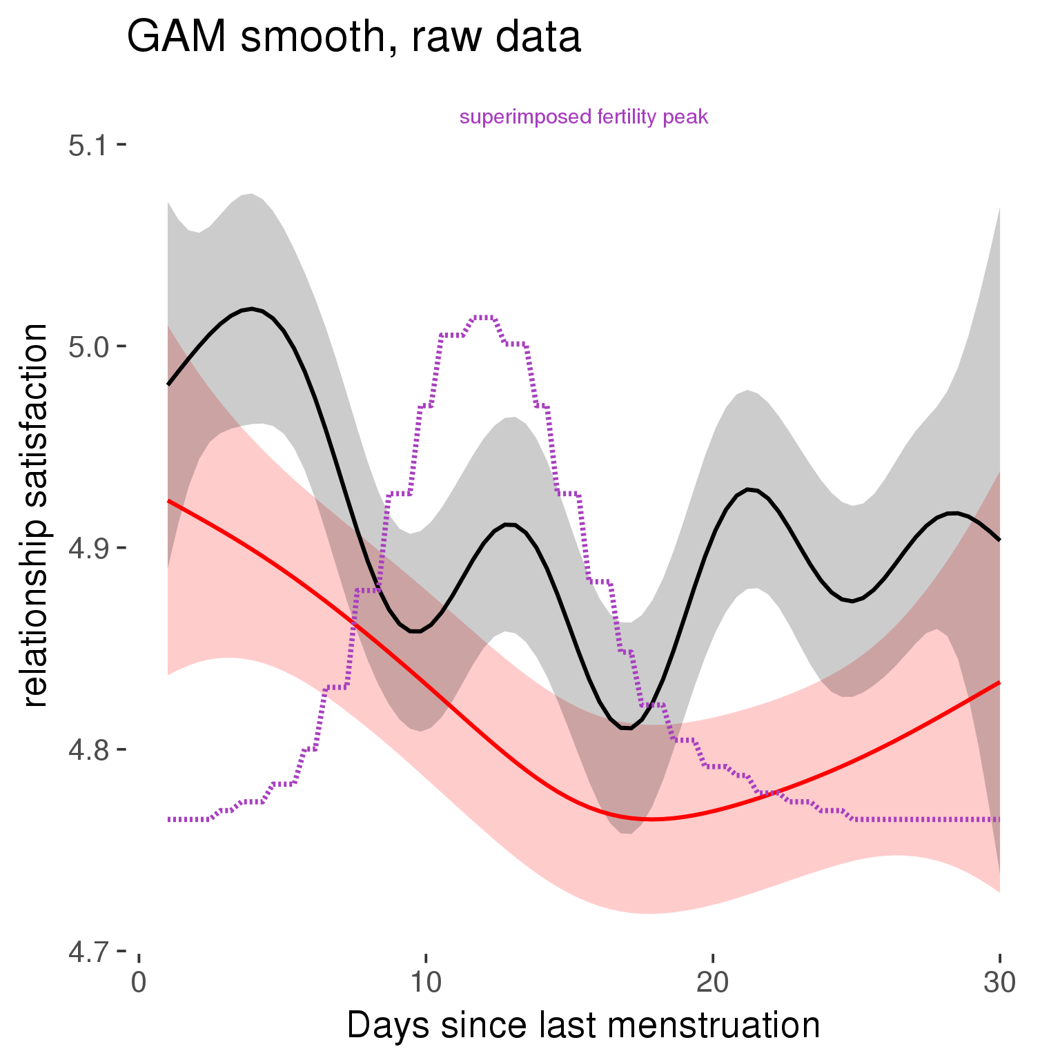
Means and standard errors over raw data
Nothing partialled out, just straight means with bootstrapped confidence intervals.
tryCatch({
trend_plot = ggplot(tmp,aes_string(x = "RCD", y = outcome, colour = "included")) +
geom_pointrange(size = 0.8, stat = 'summary', fun.data = "mean_cl_boot")
}, error = function(e){cat_message(e, "danger")})
tryCatch({
trend_data = ggplot_build(trend_plot)$data[[1]]
}, error = function(e){cat_message(e, "danger")})
trend_data$RCD = round(trend_data$x)
trend_data = left_join(trend_data, tmp %>% select(real, RCD,fertile) %>% unique(), by = "RCD")
trend_data %>%
filter(real == TRUE) %>%
mutate(superimposed = ( ( (fertile - 0.01)/0.58) * (max(y)-min(y) ) ) + min(y) ) ->
trend_data
plot3 = ggplot(trend_data) +
geom_pointrange(aes(x = x, y = y, ymin = ymin,ymax = ymax, colour = factor(group)), size = 0.8, stat = "identity", alpha = 0.6, position = position_dodge(width = .5)) +
scale_x_continuous("Days until next menstruation") +
geom_line(aes(x= x, y = superimposed), color = "#a83fbf", size = 1, linetype = 'dashed') +
annotate("text",x = mean(trend_data$x), y = max(trend_data$superimposed,na.rm=T) + 0.1, label = 'superimposed fertility peak', color = "#a83fbf") +
scale_y_continuous(outcome_label) +
ggtitle("Means with standard errors, raw data") +
scale_color_manual("Contraception status",values = c("2"="black","1"= "red"), labels = c("2"="hormonally\ncontracepting","1"="cycling"), guide = F) +
scale_fill_manual("Contraception status",values = c("2"="black","1"= "red"), labels = c("2"="hormonally\ncontracepting","1"="cycling"), guide = F)
suppressWarnings(print(plot3))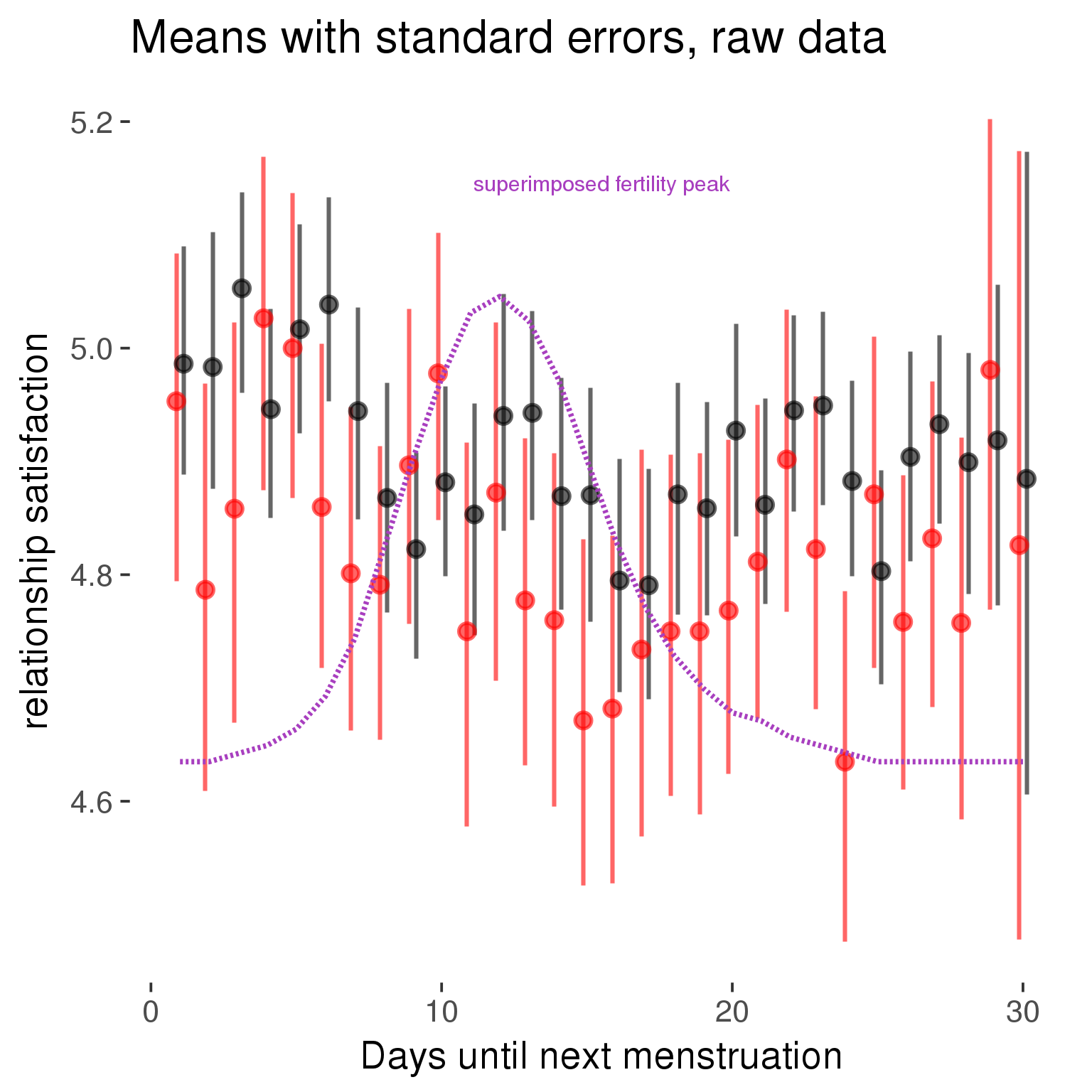
Robustness checks
M_r1: Random slopes for conception risk and menstruation
tryCatch({
# refit model with random effects for fertile and menstruation dummies
with_ind_diff = update(model, formula = . ~ . - (1| person) + (1 + fertile + menstruation | person))
# pull the random effects, format as tibble
rand = coef(with_ind_diff)$person %>%
tibble::rownames_to_column("person") %>%
mutate(person = as.numeric(person))
# pull the fixed effects
fixd = data.frame(fixef(with_ind_diff)) %>%
tibble::rownames_to_column("effect")
names(fixd) = c("effect", "pop_effect_size")
# pull apart the coefficients so that we can account for the fact that the random effect variation implicitly includes HC explaining the mean population-level effect of fertile/menstruation dummies among HC users
fixd = fixd %>%
separate(effect, c("included", "effect"), sep = ":", fill = "left") %>%
mutate(included = if_else(is.na(included), "cycling", str_replace(included, "included", "")))
fixd[2,c("included", "effect")] = c("horm_contra", "(Intercept)")
rand = rand %>%
# merge diary data on the random effects, so that we know who is a HC users and who isn't
inner_join(diary %>% select(person, included) %>% unique(), by = 'person') %>%
# gather into long format, to have the dataset by predictor
gather(effect, value, -person, -included) %>%
inner_join(fixd, by = c('effect', 'included')) %>%
# pull the fixed effects
mutate(
# only for those who are HC users, add the moderated population effect size for this effect (the random effects have the reference category mean)
value = if_else(included == "horm_contra", value + pop_effect_size, value),
effect = recode(effect, "includedhorm_contra" = "HC user",
"includedhorm_contra:fertile" = "HC user x fertile",
"includedhorm_contra:menstruationpre" = "HC user x premens.",
"includedhorm_contra:menstruationyes" = "HC user x mens.",
"menstruationyes" = "mens.",
"menstruationpre" = "premens.")) %>%
group_by(included, effect) %>%
# filter out predictors that aren't modelled as varying/random
filter(sd(value) > 0)
# plot dot plot of random effects
print(
ggplot(rand, aes(x = included, y = value, color = included, fill = included)) +
facet_wrap( ~ effect, scales = "free") +
# geom_violin(alpha = 0.4, size = 0) +
geom_dotplot(binaxis='y', dotsize = 0.1, method = "histodot") +
# geom_jitter(alpha = 0.05) +
coord_flip() +
geom_pointrange(stat = 'summary', fun.data = 'mean_sdl', color = 'darkred', size = 1.2) +
scale_color_manual("Contraception status", values = c("horm_contra"="black","cycling"= "red"), labels = c("horm_contra"="hormonally\ncontracepting","cycling"="cycling"), guide = F) +
scale_fill_manual("Contraception status", values = c("horm_contra"="black","cycling"= "red"), labels = c("horm_contra"="hormonally\ncontracepting","1"="cycling"), guide = F) +
ggtitle("M_r1: allowing participant-varying slopes", subtitle = "for the conception risk measure and the menstruation dummies") +
scale_x_discrete("Hormonal contraception", breaks = c("horm_contra", "cycling"), labels = c("yes", "no")) +
scale_y_continuous("Random effect size distribution"))
print_summary(with_ind_diff)
cat(pander(anova(model, with_ind_diff)))
}, error = function(e){
with_ind_diff = model
cat_message(e, "danger")
})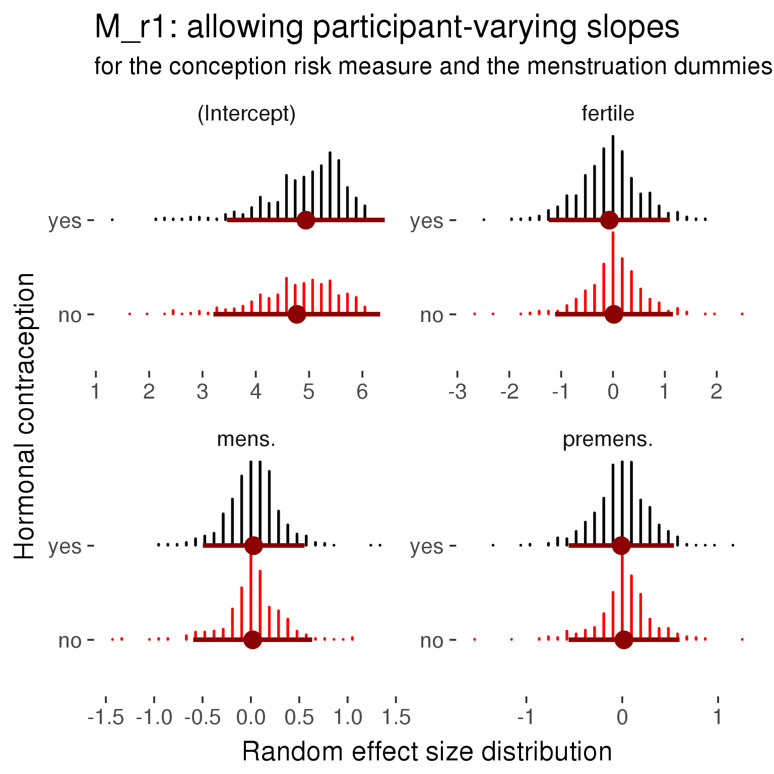
Linear mixed model fit by REML ['lmerMod']
Formula: relationship_satisfaction_1 ~ included + menstruation + fertile +
fertile_mean + (1 + fertile + menstruation | person) + included:menstruation + included:fertile
Data: diary
REML criterion at convergence: 74495
Scaled residuals:
Min 1Q Median 3Q Max
-4.885 -0.500 0.131 0.618 3.704
Random effects:
Groups Name Variance Std.Dev. Corr
person (Intercept) 0.678 0.823
fertile 0.897 0.947 -0.24
menstruationpre 0.219 0.468 -0.15 0.47
menstruationyes 0.215 0.464 -0.20 0.38 0.49
Residual 0.804 0.897
Number of obs: 26704, groups: person, 1054
Fixed effects:
Estimate Std. Error t value
(Intercept) 4.77138 0.07022 67.9
includedhorm_contra 0.16941 0.05829 2.9
menstruationpre 0.01780 0.03855 0.5
menstruationyes 0.01881 0.03694 0.5
fertile 0.01628 0.07735 0.2
fertile_mean -0.45663 0.32101 -1.4
includedhorm_contra:menstruationpre -0.02775 0.04949 -0.6
includedhorm_contra:menstruationyes 0.00992 0.04802 0.2
includedhorm_contra:fertile -0.08619 0.09835 -0.9
Correlation of Fixed Effects:
(Intr) incld_ mnstrtnp mnstrtny fertil frtl_m inclddhrm_cntr:mnstrtnp
inclddhrm_c -0.480
menstrutnpr -0.171 0.218
menstrutnys -0.194 0.238 0.433
fertile -0.188 0.299 0.456 0.376
fertile_men -0.765 -0.026 -0.013 -0.004 -0.076
inclddhrm_cntr:mnstrtnp 0.144 -0.274 -0.779 -0.337 -0.354 -0.003
inclddhrm_cntr:mnstrtny 0.155 -0.296 -0.333 -0.769 -0.289 -0.004 0.425
inclddhrm_cntr:f 0.184 -0.378 -0.358 -0.295 -0.783 0.012 0.456
inclddhrm_cntr:mnstrtny
inclddhrm_c
menstrutnpr
menstrutnys
fertile
fertile_men
inclddhrm_cntr:mnstrtnp
inclddhrm_cntr:mnstrtny
inclddhrm_cntr:f 0.372
refitting model(s) with ML (instead of REML)
| Df | AIC | BIC | logLik | deviance | Chisq | Chi Df | Pr(>Chisq) | |
|---|---|---|---|---|---|---|---|---|
| object | 11 | 75029 | 75119 | -37503 | 75007 | NA | NA | NA |
| ..1 | 20 | 74498 | 74662 | -37229 | 74458 | 549 | 9 | 1.869e-112 |
robustness_check_ovu_shift(model, diary)M_e: Exclusion criteria
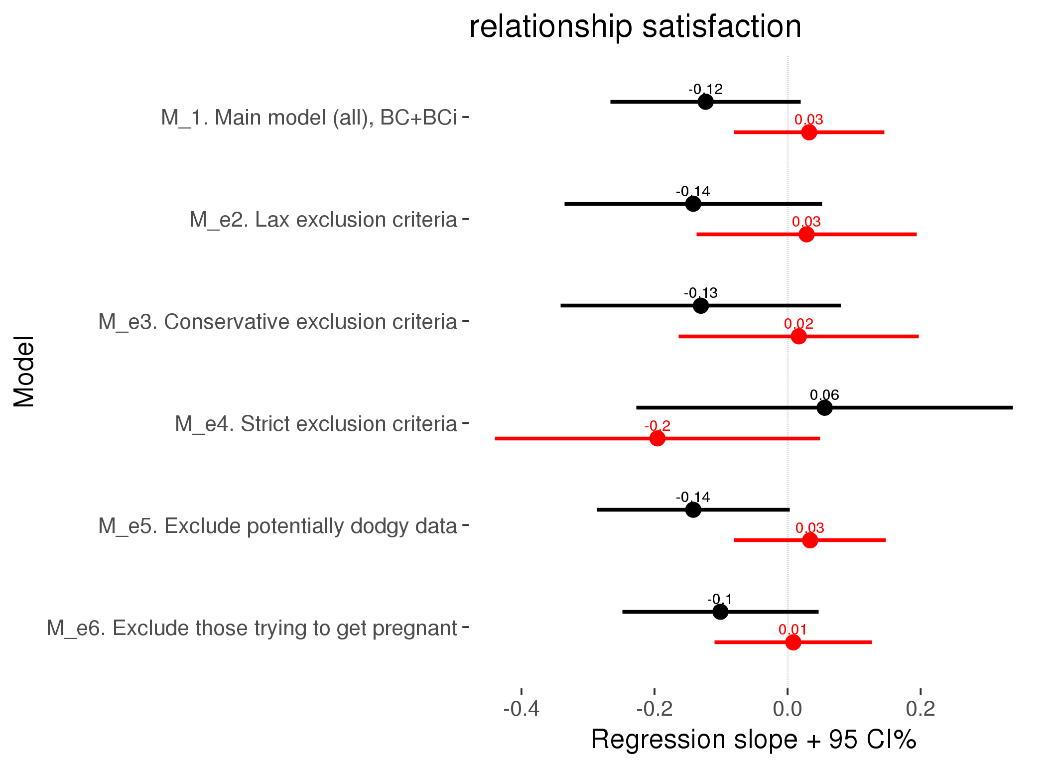
M_p: Predictors
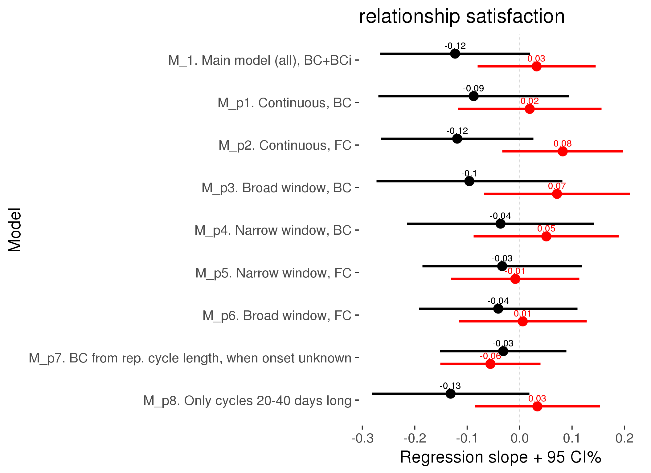
M_c: Covariates, controls, autocorrelation
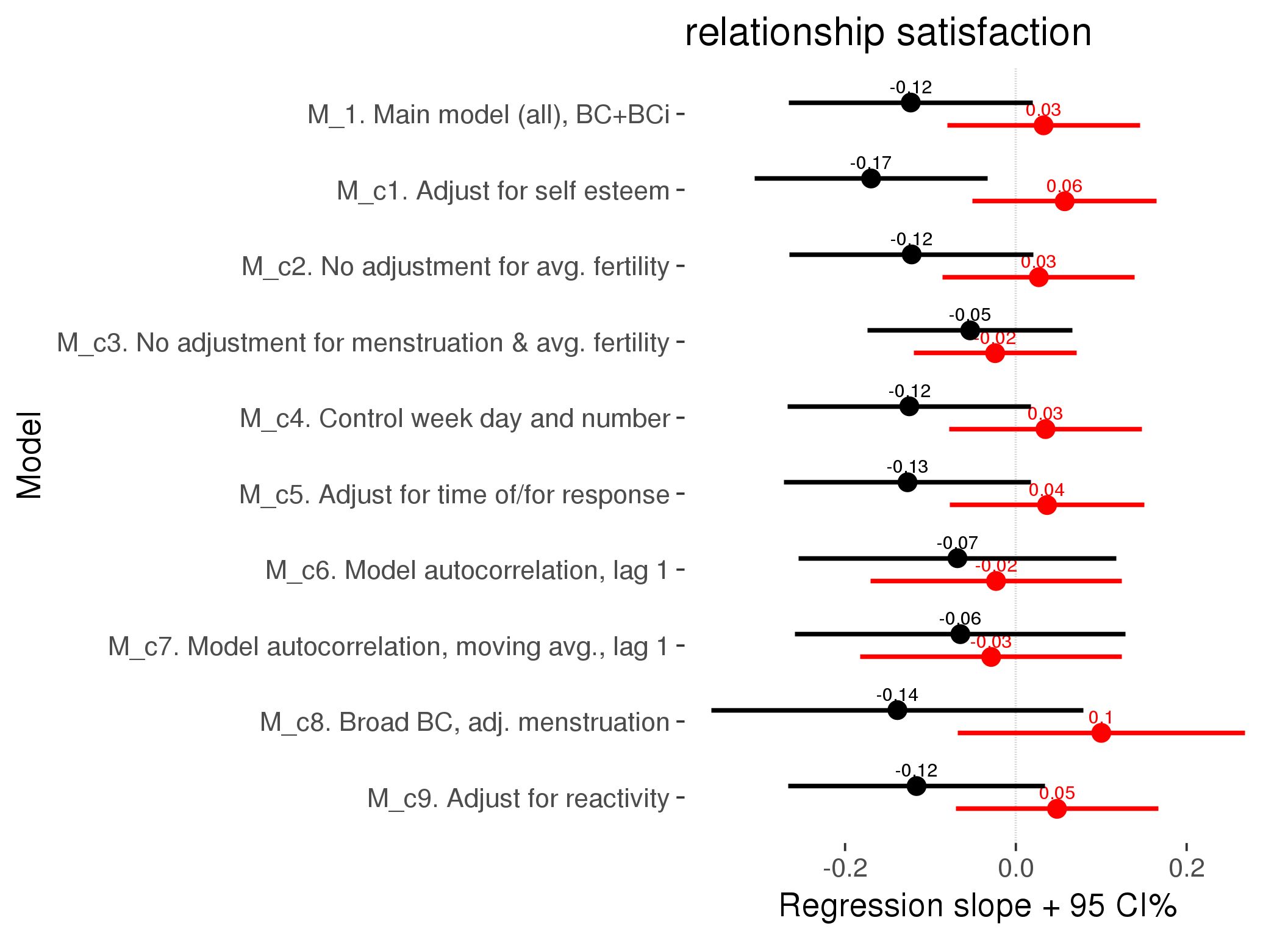
Linear mixed model fit by REML ['lmerMod']
REML criterion at convergence: 68128
Scaled residuals:
Min 1Q Median 3Q Max
-4.869 -0.513 0.151 0.642 3.931
Random effects:
Groups Name Variance Std.Dev.
person (Intercept) 0.65556 0.8097
Xr.2 s(days_filled_out):includedhorm_contra 0.00000 0.0000
Xr.1 s(days_filled_out):includedcycling 0.00532 0.0729
Xr.0 s(day_number):includedhorm_contra 0.00000 0.0000
Xr s(day_number):includedcycling 0.00000 0.0000
Residual 0.84841 0.9211
Number of obs: 24398, groups: person, 1054; Xr.2, 8; Xr.1, 8; Xr.0, 8; Xr, 8
Fixed effects:
Estimate Std. Error t value
X(Intercept) 4.74653 0.07014 67.7
Xincludedhorm_contra 0.17715 0.05791 3.1
Xmenstruationpre 0.02050 0.02940 0.7
Xmenstruationyes 0.04006 0.02823 1.4
Xfertile 0.04821 0.06049 0.8
Xfertile_mean -0.40980 0.31940 -1.3
Xincludedhorm_contra:menstruationpre -0.02291 0.03768 -0.6
Xincludedhorm_contra:menstruationyes -0.00947 0.03692 -0.3
Xincludedhorm_contra:fertile -0.11629 0.07660 -1.5
Xs(day_number):includedcyclingFx1 -0.02205 0.04809 -0.5
Xs(day_number):includedhorm_contraFx1 0.04350 0.04034 1.1
Xs(days_filled_out):includedcyclingFx1 0.02220 0.05635 0.4
Xs(days_filled_out):includedhorm_contraFx1 -0.05586 0.04137 -1.4
Family: gaussian
Link function: identity
Formula:
relationship_satisfaction_1 ~ included + menstruation + fertile +
fertile_mean + s(day_number, by = included) + s(days_filled_out,
by = included) + included:menstruation + included:fertile
Parametric coefficients:
Estimate Std. Error t value Pr(>|t|)
(Intercept) 4.74653 0.07014 67.68 <2e-16 ***
includedhorm_contra 0.17715 0.05791 3.06 0.0022 **
menstruationpre 0.02050 0.02940 0.70 0.4855
menstruationyes 0.04006 0.02823 1.42 0.1559
fertile 0.04821 0.06049 0.80 0.4255
fertile_mean -0.40980 0.31940 -1.28 0.1995
includedhorm_contra:menstruationpre -0.02291 0.03768 -0.61 0.5432
includedhorm_contra:menstruationyes -0.00947 0.03692 -0.26 0.7977
includedhorm_contra:fertile -0.11629 0.07660 -1.52 0.1290
---
Signif. codes: 0 '***' 0.001 '**' 0.01 '*' 0.05 '.' 0.1 ' ' 1
Approximate significance of smooth terms:
edf Ref.df F p-value
s(day_number):includedcycling 1.00 1.00 0.21 0.65
s(day_number):includedhorm_contra 1.00 1.00 1.16 0.28
s(days_filled_out):includedcycling 2.06 2.06 1.17 0.28
s(days_filled_out):includedhorm_contra 1.00 1.00 1.82 0.18
R-sq.(adj) = 0.00169
lmer.REML = 68127 Scale est. = 0.84841 n = 24398
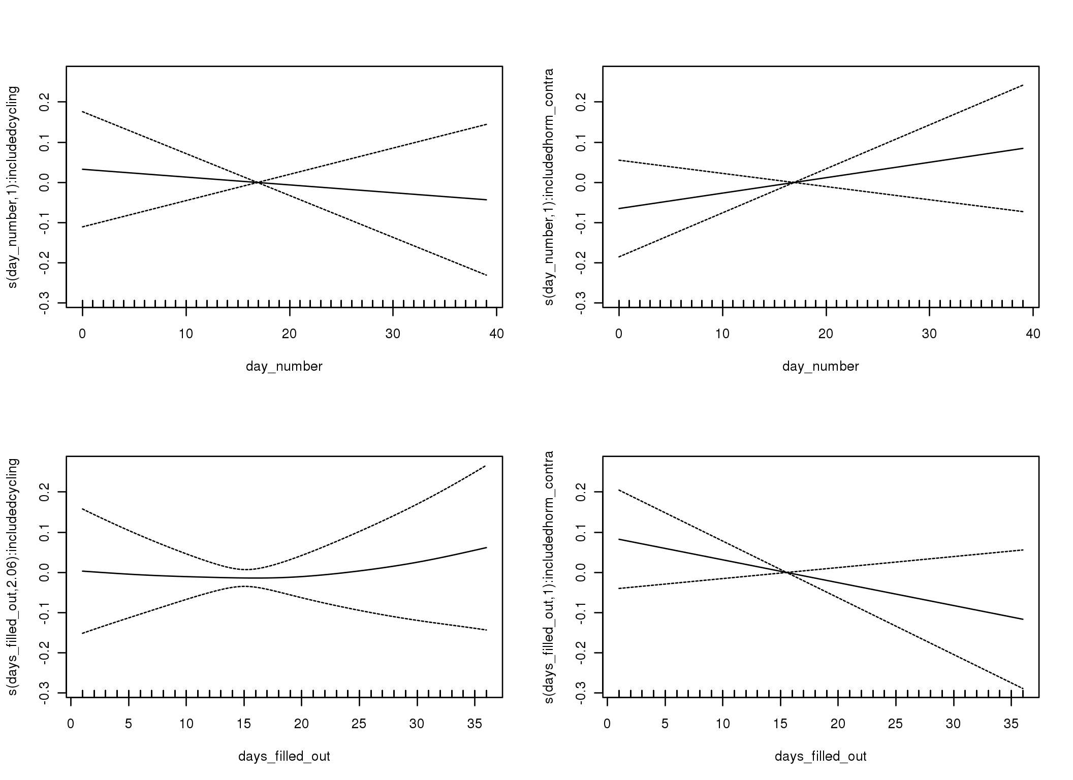
Linear mixed-effects model fit by REML
Data: diary
AIC BIC logLik
71967 72065 -35972
Random effects:
Formula: ~1 | person
(Intercept) Residual
StdDev: 0.7635 0.9562
Correlation Structure: ARMA(1,0)
Formula: ~day_number | person
Parameter estimate(s):
Phi1
0.3982
Fixed effects: relationship_satisfaction_1 ~ included * (menstruation + fertile) + fertile_mean
Value Std.Error DF t-value p-value
(Intercept) 4.782 0.0701 25644 68.25 0.0000
includedhorm_contra 0.160 0.0577 1051 2.77 0.0056
menstruationpre -0.004 0.0341 25644 -0.12 0.9046
menstruationyes -0.005 0.0317 25644 -0.16 0.8739
fertile -0.023 0.0751 25644 -0.31 0.7574
fertile_mean -0.391 0.3220 1051 -1.21 0.2250
includedhorm_contra:menstruationpre -0.013 0.0438 25644 -0.29 0.7730
includedhorm_contra:menstruationyes 0.025 0.0412 25644 0.60 0.5498
includedhorm_contra:fertile -0.068 0.0949 25644 -0.72 0.4714
Correlation:
(Intr) incld_ mnstrtnp mnstrtny fertil frtl_m inclddhrm_cntr:mnstrtnp
includedhorm_contra -0.477
menstruationpre -0.184 0.230
menstruationyes -0.182 0.226 0.406
fertile -0.178 0.298 0.402 0.345
fertile_mean -0.768 -0.027 -0.007 -0.005 -0.086
includedhorm_contra:menstruationpre 0.151 -0.287 -0.778 -0.316 -0.312 -0.004
includedhorm_contra:menstruationyes 0.145 -0.275 -0.312 -0.770 -0.265 -0.003 0.391
includedhorm_contra:fertile 0.181 -0.377 -0.317 -0.273 -0.786 0.015 0.400
inclddhrm_cntr:mnstrtny
includedhorm_contra
menstruationpre
menstruationyes
fertile
fertile_mean
includedhorm_contra:menstruationpre
includedhorm_contra:menstruationyes
includedhorm_contra:fertile 0.338
Standardized Within-Group Residuals:
Min Q1 Med Q3 Max
-4.7551 -0.4926 0.1623 0.6415 3.6946
Number of Observations: 26704
Number of Groups: 1054
Linear mixed-effects model fit by REML
Data: diary
AIC BIC logLik
71785 71892 -35880
Random effects:
Formula: ~1 | person
(Intercept) Residual
StdDev: 0.7486 0.9652
Correlation Structure: ARMA(1,1)
Formula: ~day_number | person
Parameter estimate(s):
Phi1 Theta1
0.6182 -0.2594
Fixed effects: relationship_satisfaction_1 ~ included * (menstruation + fertile) + fertile_mean
Value Std.Error DF t-value p-value
(Intercept) 4.782 0.0701 25644 68.17 0.0000
includedhorm_contra 0.159 0.0578 1051 2.75 0.0061
menstruationpre -0.001 0.0344 25644 -0.04 0.9698
menstruationyes -0.010 0.0322 25644 -0.31 0.7564
fertile -0.029 0.0782 25644 -0.37 0.7114
fertile_mean -0.371 0.3230 1051 -1.15 0.2505
includedhorm_contra:menstruationpre -0.017 0.0442 25644 -0.39 0.6932
includedhorm_contra:menstruationyes 0.028 0.0418 25644 0.67 0.5028
includedhorm_contra:fertile -0.065 0.0988 25644 -0.66 0.5107
Correlation:
(Intr) incld_ mnstrtnp mnstrtny fertil frtl_m inclddhrm_cntr:mnstrtnp
includedhorm_contra -0.476
menstruationpre -0.184 0.227
menstruationyes -0.185 0.229 0.421
fertile -0.178 0.303 0.365 0.332
fertile_mean -0.768 -0.029 -0.004 -0.005 -0.090
includedhorm_contra:menstruationpre 0.149 -0.283 -0.778 -0.327 -0.283 -0.004
includedhorm_contra:menstruationyes 0.147 -0.278 -0.325 -0.772 -0.256 -0.003 0.408
includedhorm_contra:fertile 0.183 -0.382 -0.288 -0.263 -0.786 0.016 0.363
inclddhrm_cntr:mnstrtny
includedhorm_contra
menstruationpre
menstruationyes
fertile
fertile_mean
includedhorm_contra:menstruationpre
includedhorm_contra:menstruationyes
includedhorm_contra:fertile 0.325
Standardized Within-Group Residuals:
Min Q1 Med Q3 Max
-4.7014 -0.4824 0.1662 0.6383 3.5874
Number of Observations: 26704
Number of Groups: 1054
M_d: Other designs
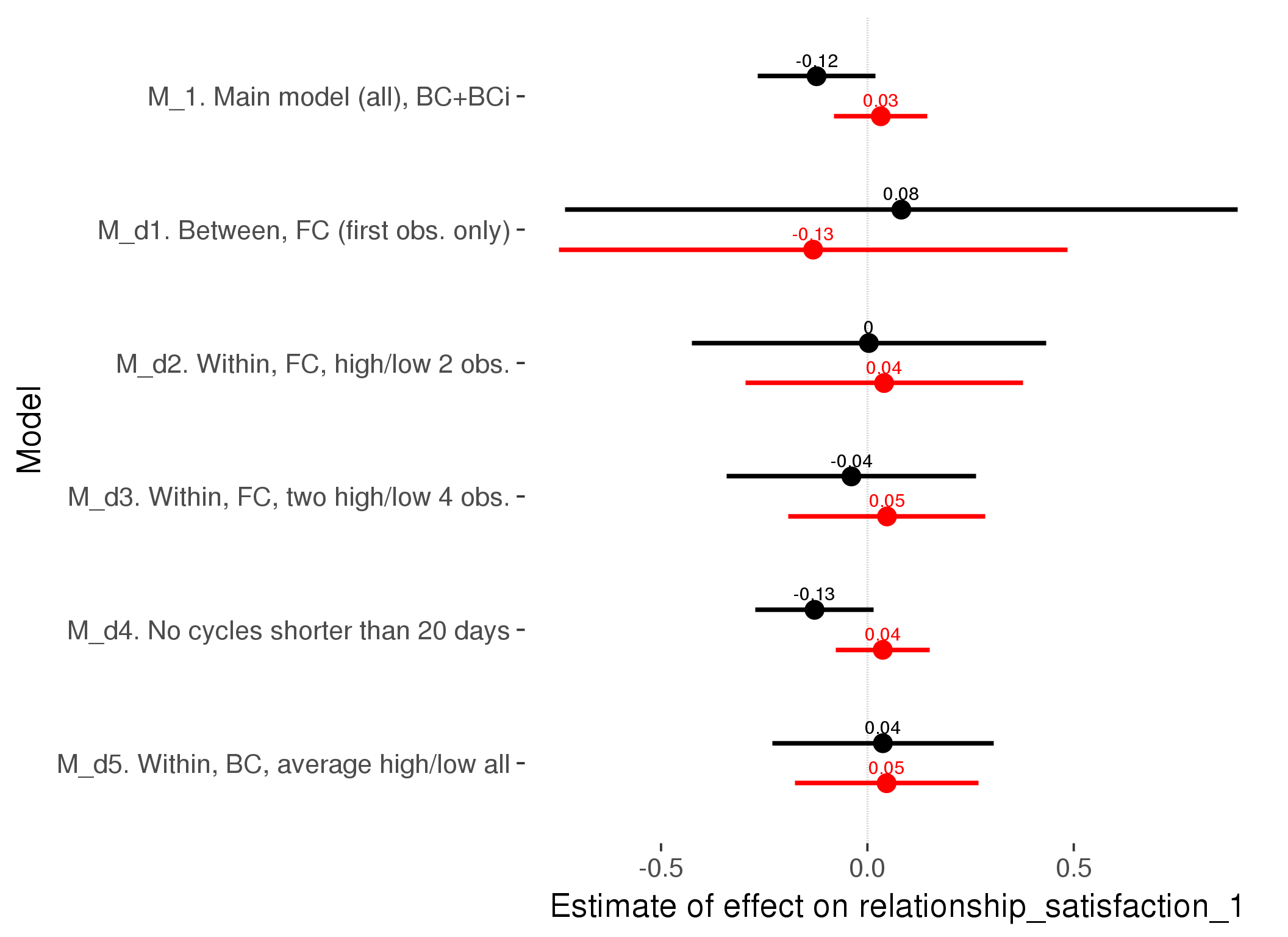
M_m1: Moderation by contraceptive method
Based on the sample with lax exclusion criteria. Users who used any hormonal contraception are classified as hormonal, users who use any awareness-based methods (counting, temperature-based) are classified as ‘fertility-awareness’, women who don’t fall into the before groups and use condoms, pessars, coitus interruptus etc. are classified as ‘barrie or abstinence’. Women who don’t use contraception or use other methods such as sterilisation are excluded from this analysis.
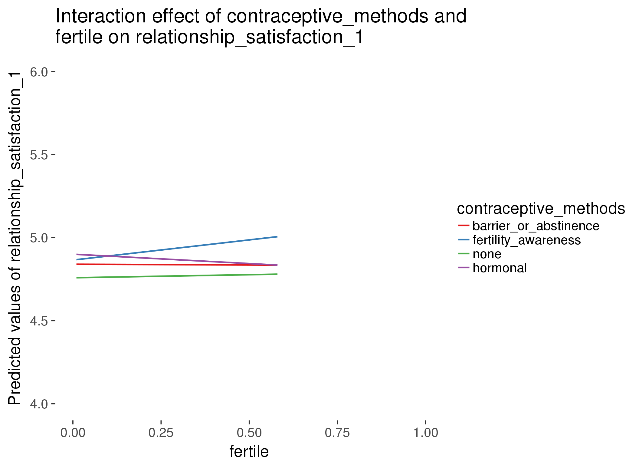

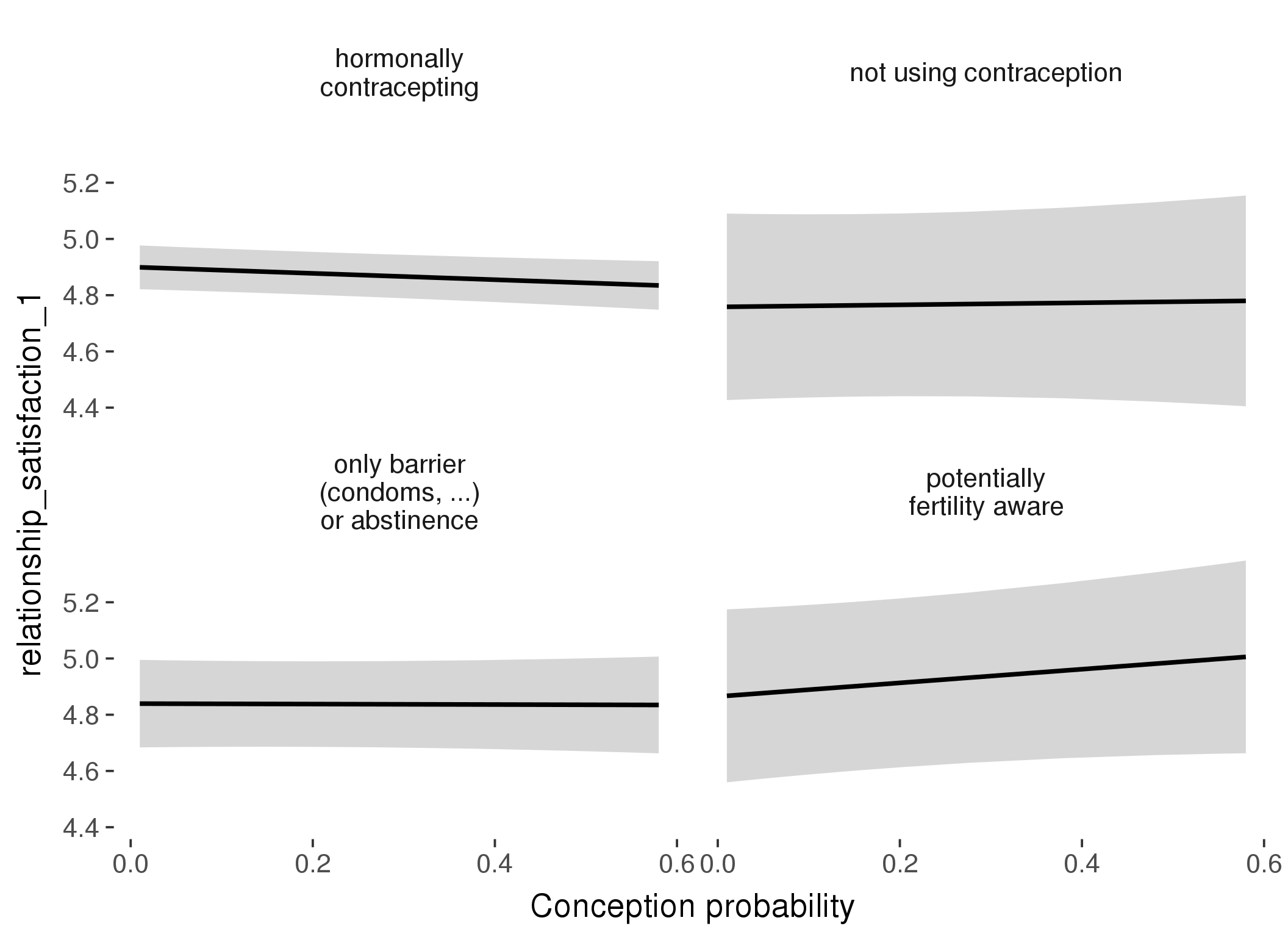
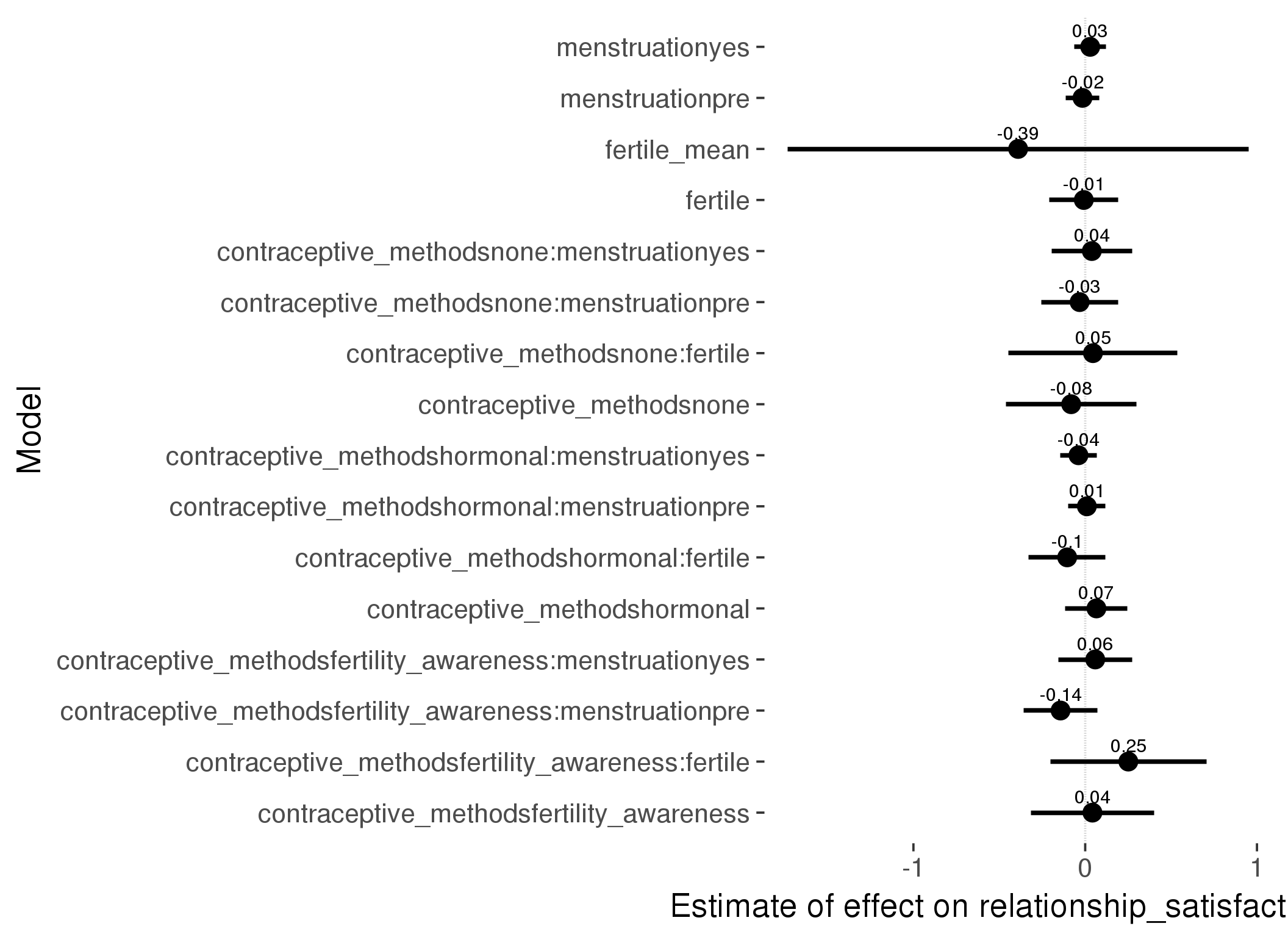
Linear mixed model fit by REML ['lmerMod']
Formula: relationship_satisfaction_1 ~ fertile_mean + (1 | person) + contraceptive_methods +
fertile + menstruation + fertile:contraceptive_methods + menstruation:contraceptive_methods
Data: diary
Subset: !is.na(included_lax) & contraceptive_method != "other"
REML criterion at convergence: 46954
Scaled residuals:
Min 1Q Median 3Q Max
-4.946 -0.507 0.136 0.662 3.917
Random effects:
Groups Name Variance Std.Dev.
person (Intercept) 0.536 0.732
Residual 0.837 0.915
Number of obs: 17044, groups: person, 513
Fixed effects:
Estimate Std. Error t value
(Intercept) 4.90611 0.14095 34.8
fertile_mean -0.39045 0.68497 -0.6
contraceptive_methodsfertility_awareness 0.04214 0.18352 0.2
contraceptive_methodsnone -0.08171 0.19453 -0.4
contraceptive_methodshormonal 0.06537 0.09251 0.7
fertile -0.00823 0.10207 -0.1
menstruationpre -0.01576 0.04926 -0.3
menstruationyes 0.02907 0.04706 0.6
contraceptive_methodsfertility_awareness:fertile 0.25109 0.23180 1.1
contraceptive_methodsnone:fertile 0.04515 0.25094 0.2
contraceptive_methodshormonal:fertile -0.10485 0.11401 -0.9
contraceptive_methodsfertility_awareness:menstruationpre -0.14348 0.10918 -1.3
contraceptive_methodsnone:menstruationpre -0.03247 0.11415 -0.3
contraceptive_methodshormonal:menstruationpre 0.00961 0.05549 0.2
contraceptive_methodsfertility_awareness:menstruationyes 0.05853 0.10973 0.5
contraceptive_methodsnone:menstruationyes 0.03853 0.11937 0.3
contraceptive_methodshormonal:menstruationyes -0.03916 0.05366 -0.7
refitting model(s) with ML (instead of REML)
| Df | AIC | BIC | logLik | deviance | Chisq | Chi Df | Pr(>Chisq) | |
|---|---|---|---|---|---|---|---|---|
| add_main | 13 | 46934 | 47035 | -23454 | 46908 | NA | NA | NA |
| by_method | 19 | 46940 | 47087 | -23451 | 46902 | 6.321 | 6 | 0.3882 |
M_m2: Moderation by participant age
model %>%
test_moderator("age_group", diary, xlevels = 5)refitting model(s) with ML (instead of REML)
| Df | AIC | BIC | logLik | deviance | Chisq | Chi Df | Pr(>Chisq) | |
|---|---|---|---|---|---|---|---|---|
| with_main | 19 | 75039 | 75194 | -37500 | 75001 | NA | NA | NA |
| with_mod | 27 | 75038 | 75259 | -37492 | 74984 | 16.93 | 8 | 0.03088 |
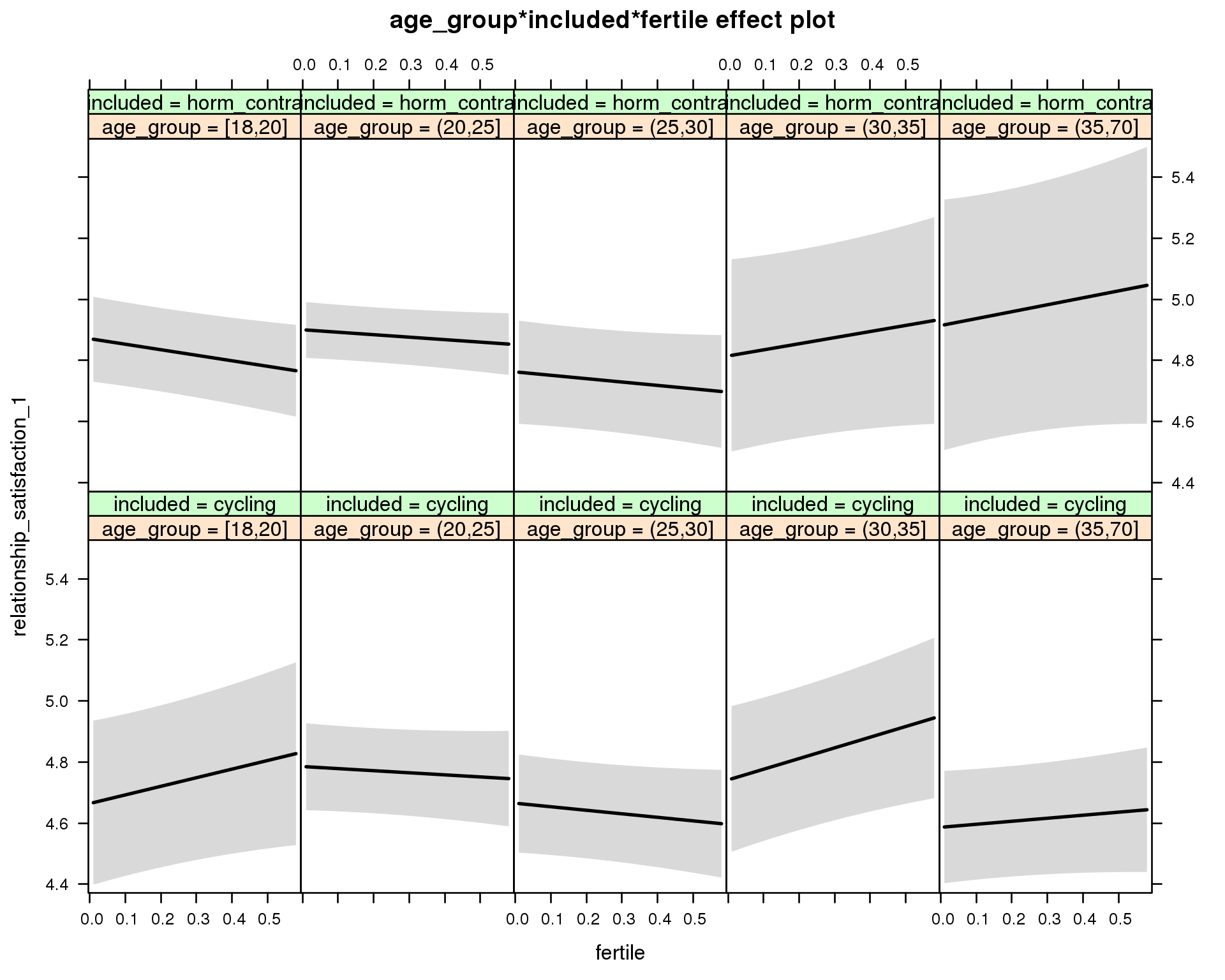
Linear mixed model fit by REML ['lmerMod']
Formula: relationship_satisfaction_1 ~ menstruation + fertile_mean + (1 |
person) + age_group + included + fertile + menstruation:included +
age_group:included + age_group:fertile + included:fertile + age_group:included:fertile
Data: diary
REML criterion at convergence: 75060
Scaled residuals:
Min 1Q Median 3Q Max
-4.872 -0.496 0.150 0.646 3.830
Random effects:
Groups Name Variance Std.Dev.
person (Intercept) 0.637 0.798
Residual 0.872 0.934
Number of obs: 26704, groups: person, 1054
Fixed effects:
Estimate Std. Error t value
(Intercept) 4.736720 0.144939 32.7
menstruationpre 0.022396 0.028509 0.8
menstruationyes 0.022796 0.026876 0.8
fertile_mean -0.463372 0.317574 -1.5
age_group(20,25] 0.121108 0.155244 0.8
age_group(25,30] 0.000916 0.159792 0.0
age_group(30,35] 0.077271 0.183357 0.4
age_group(35,70] -0.077947 0.166045 -0.5
includedhorm_contra 0.214326 0.155496 1.4
fertile 0.281634 0.164519 1.7
menstruationpre:includedhorm_contra -0.038694 0.036601 -1.1
menstruationyes:includedhorm_contra -0.004773 0.035217 -0.1
age_group(20,25]:includedhorm_contra -0.091735 0.177072 -0.5
age_group(25,30]:includedhorm_contra -0.109667 0.195009 -0.6
age_group(30,35]:includedhorm_contra -0.133834 0.253969 -0.5
age_group(35,70]:includedhorm_contra 0.121074 0.276947 0.4
age_group(20,25]:fertile -0.349835 0.182241 -1.9
age_group(25,30]:fertile -0.397189 0.187855 -2.1
age_group(30,35]:fertile 0.068435 0.217597 0.3
age_group(35,70]:fertile -0.182565 0.196345 -0.9
includedhorm_contra:fertile -0.462400 0.182452 -2.5
age_group(20,25]:includedhorm_contra:fertile 0.449493 0.204125 2.2
age_group(25,30]:includedhorm_contra:fertile 0.467346 0.226218 2.1
age_group(30,35]:includedhorm_contra:fertile 0.312544 0.292003 1.1
age_group(35,70]:includedhorm_contra:fertile 0.590339 0.331740 1.8
M_m3: Moderation by weekend
model %>%
test_moderator("weekend", diary, xlevels = 2) refitting model(s) with ML (instead of REML)
| Df | AIC | BIC | logLik | deviance | Chisq | Chi Df | Pr(>Chisq) | |
|---|---|---|---|---|---|---|---|---|
| with_main | 13 | 75011 | 75118 | -37493 | 74985 | NA | NA | NA |
| with_mod | 15 | 75013 | 75136 | -37492 | 74983 | 2.026 | 2 | 0.3631 |
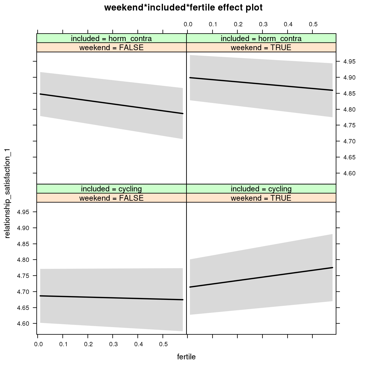
Linear mixed model fit by REML ['lmerMod']
Formula: relationship_satisfaction_1 ~ menstruation + fertile_mean + (1 |
person) + weekend + included + fertile + menstruation:included +
weekend:included + weekend:fertile + included:fertile + weekend:included:fertile
Data: diary
REML criterion at convergence: 75043
Scaled residuals:
Min 1Q Median 3Q Max
-4.850 -0.493 0.151 0.647 3.861
Random effects:
Groups Name Variance Std.Dev.
person (Intercept) 0.635 0.797
Residual 0.872 0.934
Number of obs: 26704, groups: person, 1054
Fixed effects:
Estimate Std. Error t value
(Intercept) 4.75920 0.06971 68.3
menstruationpre 0.02182 0.02850 0.8
menstruationyes 0.02383 0.02685 0.9
fertile_mean -0.46301 0.31586 -1.5
weekendTRUE 0.02637 0.02483 1.1
includedhorm_contra 0.16932 0.05799 2.9
fertile -0.02118 0.06997 -0.3
menstruationpre:includedhorm_contra -0.03765 0.03658 -1.0
menstruationyes:includedhorm_contra -0.00397 0.03519 -0.1
weekendTRUE:includedhorm_contra 0.02459 0.03195 0.8
weekendTRUE:fertile 0.12824 0.09632 1.3
includedhorm_contra:fertile -0.08609 0.08890 -1.0
weekendTRUE:includedhorm_contra:fertile -0.09023 0.12249 -0.7
M_m4: Moderation by weekday
model %>%
test_moderator("weekday", diary, xlevels = 7)refitting model(s) with ML (instead of REML)
| Df | AIC | BIC | logLik | deviance | Chisq | Chi Df | Pr(>Chisq) | |
|---|---|---|---|---|---|---|---|---|
| with_main | 23 | 74967 | 75155 | -37460 | 74921 | NA | NA | NA |
| with_mod | 35 | 74981 | 75268 | -37456 | 74911 | 9.595 | 12 | 0.6514 |
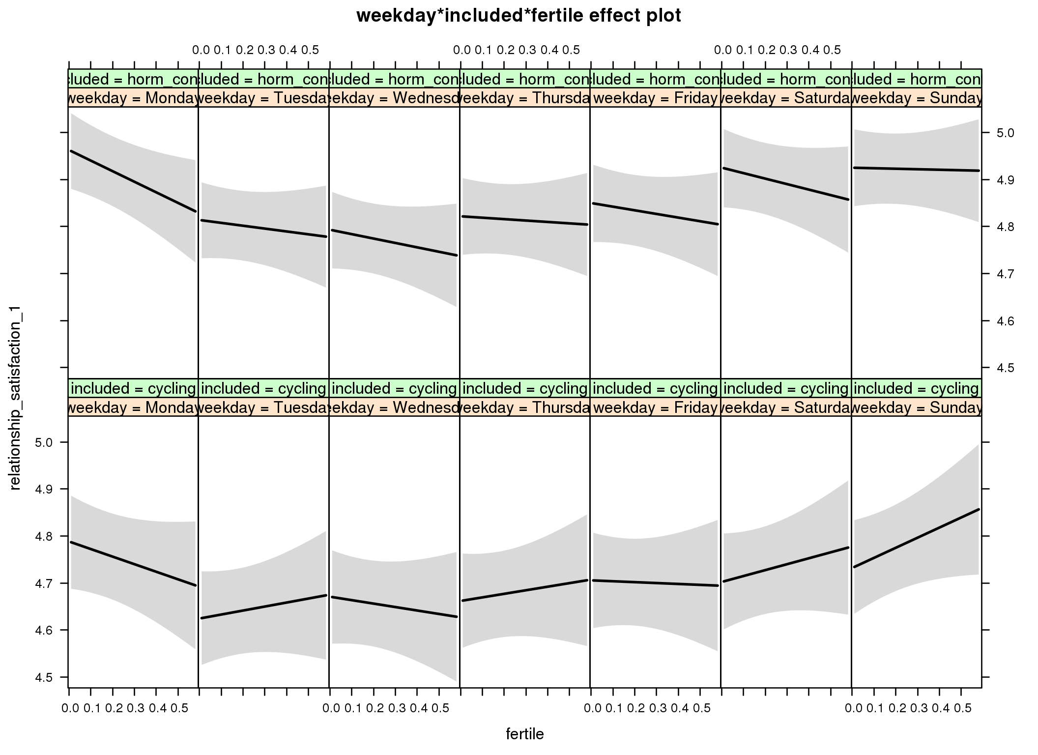
Linear mixed model fit by REML ['lmerMod']
Formula: relationship_satisfaction_1 ~ menstruation + fertile_mean + (1 |
person) + weekday + included + fertile + menstruation:included +
weekday:included + weekday:fertile + included:fertile + weekday:included:fertile
Data: diary
REML criterion at convergence: 75045
Scaled residuals:
Min 1Q Median 3Q Max
-4.828 -0.495 0.151 0.643 3.770
Random effects:
Groups Name Variance Std.Dev.
person (Intercept) 0.635 0.797
Residual 0.870 0.933
Number of obs: 26704, groups: person, 1054
Fixed effects:
Estimate Std. Error t value
(Intercept) 4.86322 0.07477 65.0
menstruationpre 0.02117 0.02847 0.7
menstruationyes 0.02315 0.02683 0.9
fertile_mean -0.47555 0.31578 -1.5
weekdayTuesday -0.16381 0.04437 -3.7
weekdayWednesday -0.11743 0.04433 -2.6
weekdayThursday -0.12646 0.04483 -2.8
weekdayFriday -0.08263 0.04558 -1.8
weekdaySaturday -0.08609 0.04605 -1.9
weekdaySunday -0.05631 0.04450 -1.3
includedhorm_contra 0.18089 0.06751 2.7
fertile -0.16091 0.12505 -1.3
menstruationpre:includedhorm_contra -0.03559 0.03655 -1.0
menstruationyes:includedhorm_contra -0.00182 0.03516 -0.1
weekdayTuesday:includedhorm_contra 0.01501 0.05701 0.3
weekdayWednesday:includedhorm_contra -0.05209 0.05722 -0.9
weekdayThursday:includedhorm_contra -0.01443 0.05777 -0.2
weekdayFriday:includedhorm_contra -0.03005 0.05854 -0.5
weekdaySaturday:includedhorm_contra 0.04863 0.05923 0.8
weekdaySunday:includedhorm_contra 0.01866 0.05742 0.3
weekdayTuesday:fertile 0.24598 0.17211 1.4
weekdayWednesday:fertile 0.08751 0.17295 0.5
weekdayThursday:fertile 0.23684 0.17543 1.4
weekdayFriday:fertile 0.14169 0.17571 0.8
weekdaySaturday:fertile 0.28696 0.17807 1.6
weekdaySunday:fertile 0.37558 0.17305 2.2
includedhorm_contra:fertile -0.06390 0.15996 -0.4
weekdayTuesday:includedhorm_contra:fertile -0.08208 0.21968 -0.4
weekdayWednesday:includedhorm_contra:fertile 0.04361 0.22143 0.2
weekdayThursday:includedhorm_contra:fertile -0.04216 0.22322 -0.2
weekdayFriday:includedhorm_contra:fertile 0.00559 0.22385 0.0
weekdaySaturday:includedhorm_contra:fertile -0.17903 0.22712 -0.8
weekdaySunday:includedhorm_contra:fertile -0.16154 0.22103 -0.7
M_m5: Moderation by exclusion threshold
model %>%
test_moderator("included_levels", diary, xlevels = 4)refitting model(s) with ML (instead of REML)
| Df | AIC | BIC | logLik | deviance | Chisq | Chi Df | Pr(>Chisq) | |
|---|---|---|---|---|---|---|---|---|
| with_main | 17 | 75023 | 75162 | -37494 | 74989 | NA | NA | NA |
| with_mod | 23 | 75028 | 75216 | -37491 | 74982 | 6.84 | 6 | 0.3359 |
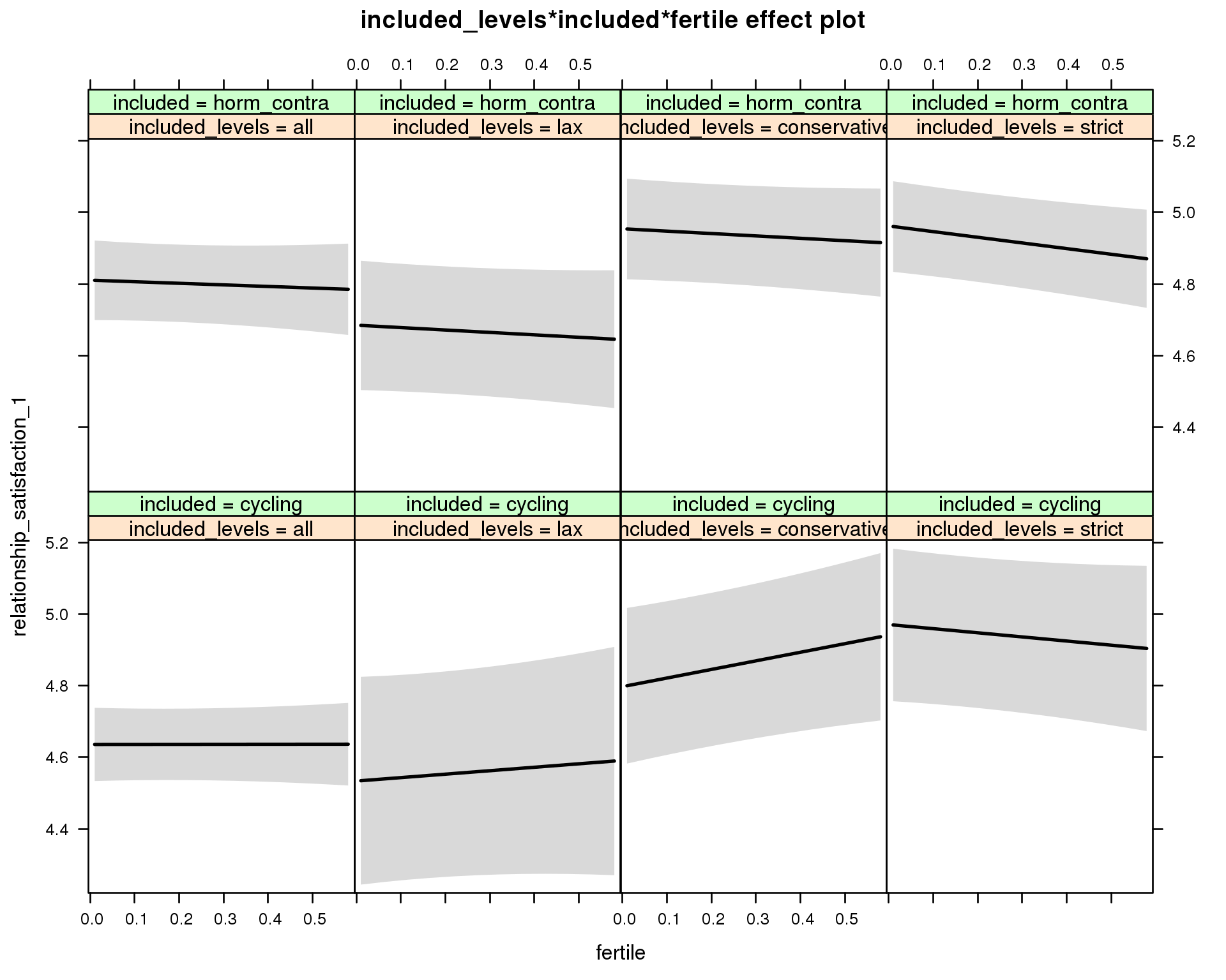
Linear mixed model fit by REML ['lmerMod']
Formula: relationship_satisfaction_1 ~ menstruation + fertile_mean + (1 |
person) + included_levels + included + fertile + menstruation:included +
included_levels:included + included_levels:fertile + included:fertile +
included_levels:included:fertile
Data: diary
REML criterion at convergence: 75054
Scaled residuals:
Min 1Q Median 3Q Max
-4.860 -0.494 0.152 0.651 3.846
Random effects:
Groups Name Variance Std.Dev.
person (Intercept) 0.627 0.792
Residual 0.872 0.934
Number of obs: 26704, groups: person, 1054
Fixed effects:
Estimate Std. Error t value
(Intercept) 4.70797 0.07620 61.8
menstruationpre 0.02159 0.02853 0.8
menstruationyes 0.02440 0.02687 0.9
fertile_mean -0.46168 0.31709 -1.5
included_levelslax -0.10233 0.15713 -0.7
included_levelsconservative 0.16157 0.12260 1.3
included_levelsstrict 0.33496 0.12063 2.8
includedhorm_contra 0.18280 0.07867 2.3
fertile 0.00110 0.07274 0.0
menstruationpre:includedhorm_contra -0.03868 0.03664 -1.1
menstruationyes:includedhorm_contra -0.00665 0.03524 -0.2
included_levelslax:includedhorm_contra -0.02343 0.19118 -0.1
included_levelsconservative:includedhorm_contra -0.01796 0.15306 -0.1
included_levelsstrict:includedhorm_contra -0.18358 0.14819 -1.2
included_levelslax:fertile 0.09536 0.17761 0.5
included_levelsconservative:fertile 0.23890 0.13265 1.8
included_levelsstrict:fertile -0.11628 0.13272 -0.9
includedhorm_contra:fertile -0.04509 0.11112 -0.4
included_levelslax:includedhorm_contra:fertile -0.11892 0.21669 -0.5
included_levelsconservative:includedhorm_contra:fertile -0.26158 0.17249 -1.5
included_levelsstrict:includedhorm_contra:fertile 0.00228 0.16982 0.0
M_m6: Moderation by cycle length
model %>%
test_moderator("cycle_length_groups", diary, xlevels = 4)refitting model(s) with ML (instead of REML)
| Df | AIC | BIC | logLik | deviance | Chisq | Chi Df | Pr(>Chisq) | |
|---|---|---|---|---|---|---|---|---|
| with_main | 17 | 75018 | 75157 | -37492 | 74984 | NA | NA | NA |
| with_mod | 23 | 75026 | 75215 | -37490 | 74980 | 3.662 | 6 | 0.7224 |
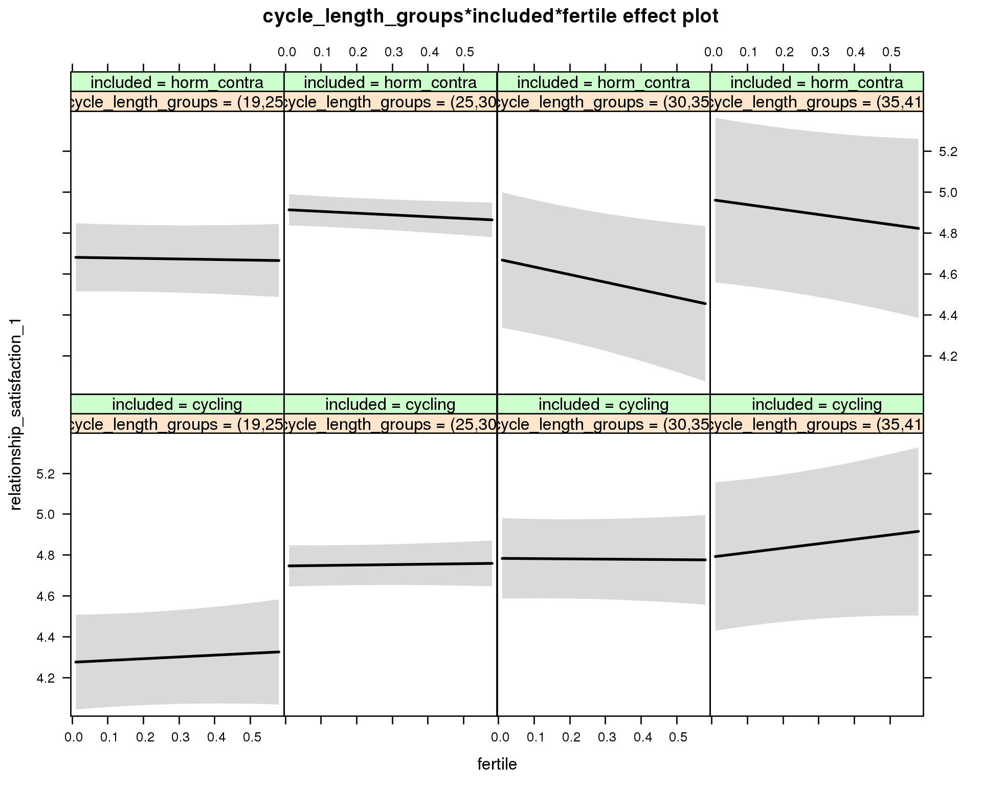
Linear mixed model fit by REML ['lmerMod']
Formula: relationship_satisfaction_1 ~ menstruation + fertile_mean + (1 |
person) + cycle_length_groups + included + fertile + menstruation:included +
cycle_length_groups:included + cycle_length_groups:fertile +
included:fertile + cycle_length_groups:included:fertile
Data: diary
REML criterion at convergence: 75044
Scaled residuals:
Min 1Q Median 3Q Max
-4.873 -0.496 0.150 0.646 3.819
Random effects:
Groups Name Variance Std.Dev.
person (Intercept) 0.626 0.791
Residual 0.872 0.934
Number of obs: 26704, groups: person, 1054
Fixed effects:
Estimate Std. Error t value
(Intercept) 4.34296 0.13142 33.0
menstruationpre 0.02137 0.02855 0.7
menstruationyes 0.02321 0.02706 0.9
fertile_mean -0.42919 0.31813 -1.3
cycle_length_groups(25,30] 0.47102 0.12917 3.6
cycle_length_groups(30,35] 0.50806 0.15543 3.3
cycle_length_groups(35,41] 0.51485 0.22023 2.3
includedhorm_contra 0.41173 0.14679 2.8
fertile 0.08695 0.15188 0.6
menstruationpre:includedhorm_contra -0.03589 0.03663 -1.0
menstruationyes:includedhorm_contra -0.00405 0.03541 -0.1
cycle_length_groups(25,30]:includedhorm_contra -0.23801 0.15949 -1.5
cycle_length_groups(30,35]:includedhorm_contra -0.51796 0.24489 -2.1
cycle_length_groups(35,41]:includedhorm_contra -0.23322 0.31271 -0.7
cycle_length_groups(25,30]:fertile -0.06549 0.16295 -0.4
cycle_length_groups(30,35]:fertile -0.09967 0.19292 -0.5
cycle_length_groups(35,41]:fertile 0.12899 0.27253 0.5
includedhorm_contra:fertile -0.11422 0.17929 -0.6
cycle_length_groups(25,30]:includedhorm_contra:fertile 0.00681 0.19304 0.0
cycle_length_groups(30,35]:includedhorm_contra:fertile -0.24656 0.30377 -0.8
cycle_length_groups(35,41]:includedhorm_contra:fertile -0.34360 0.35880 -1.0
M_m7: Moderation by certainty about menstruation parameters
model %>%
test_moderator("certainty_menstruation", diary)refitting model(s) with ML (instead of REML)
| Df | AIC | BIC | logLik | deviance | Chisq | Chi Df | Pr(>Chisq) | |
|---|---|---|---|---|---|---|---|---|
| with_main | 13 | 75031 | 75137 | -37502 | 75005 | NA | NA | NA |
| with_mod | 15 | 75031 | 75154 | -37501 | 75001 | 3.617 | 2 | 0.1639 |
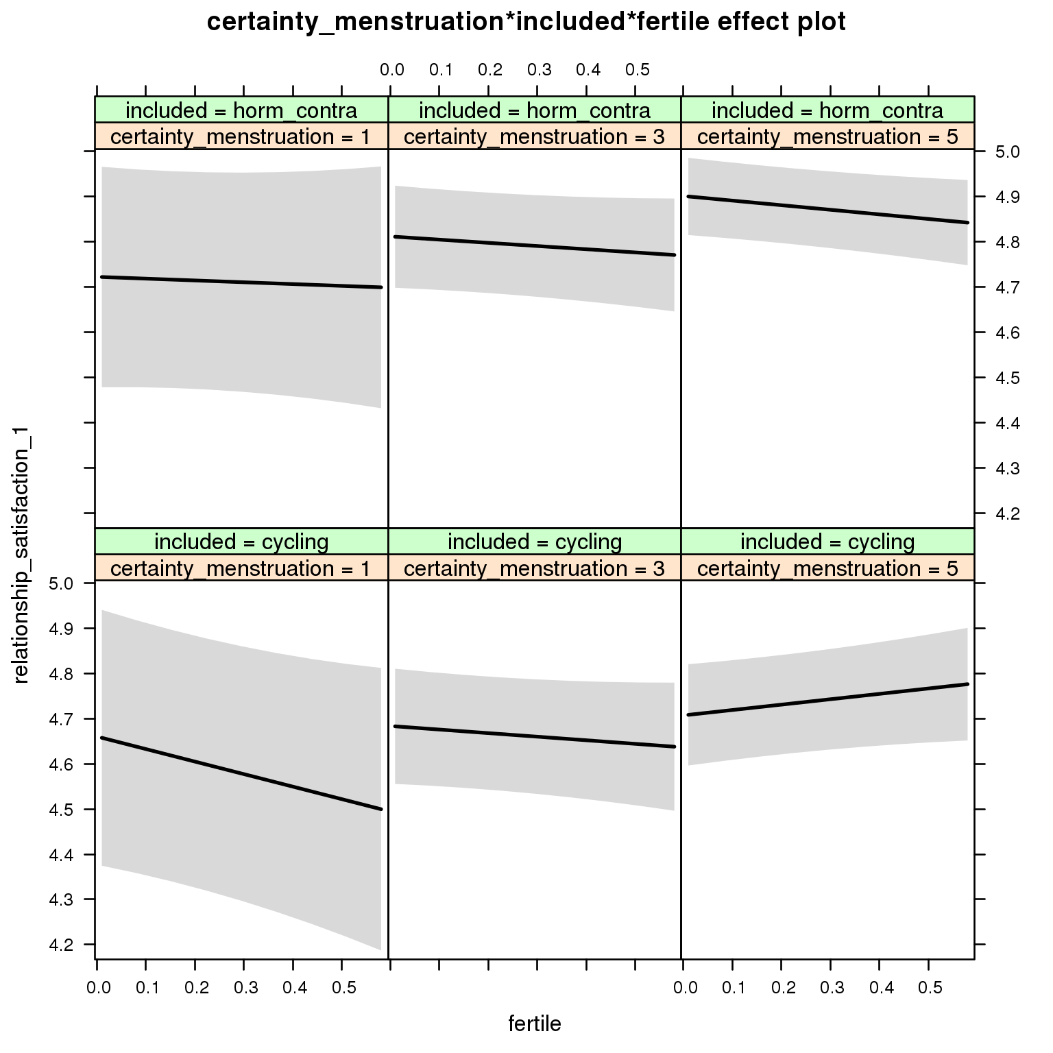
Linear mixed model fit by REML ['lmerMod']
Formula: relationship_satisfaction_1 ~ menstruation + fertile_mean + (1 |
person) + certainty_menstruation + included + fertile + menstruation:included +
certainty_menstruation:included + certainty_menstruation:fertile +
included:fertile + certainty_menstruation:included:fertile
Data: diary
REML criterion at convergence: 75060
Scaled residuals:
Min 1Q Median 3Q Max
-4.876 -0.497 0.152 0.646 3.834
Random effects:
Groups Name Variance Std.Dev.
person (Intercept) 0.636 0.797
Residual 0.872 0.934
Number of obs: 26704, groups: person, 1054
Fixed effects:
Estimate Std. Error t value
(Intercept) 4.72462 0.19467 24.27
menstruationpre 0.02363 0.02852 0.83
menstruationyes 0.02677 0.02690 1.00
fertile_mean -0.48796 0.31650 -1.54
certainty_menstruation 0.01172 0.04438 0.26
includedhorm_contra 0.03744 0.24715 0.15
fertile -0.37640 0.22650 -1.66
menstruationpre:includedhorm_contra -0.03894 0.03661 -1.06
menstruationyes:includedhorm_contra -0.00775 0.03524 -0.22
certainty_menstruation:includedhorm_contra 0.03300 0.05757 0.57
certainty_menstruation:fertile 0.09911 0.05307 1.87
includedhorm_contra:fertile 0.35171 0.29435 1.19
certainty_menstruation:includedhorm_contra:fertile -0.11449 0.06803 -1.68
M_m8: Moderation by cycle regularity
model %>%
test_moderator("cycle_regularity", diary)refitting model(s) with ML (instead of REML)
| Df | AIC | BIC | logLik | deviance | Chisq | Chi Df | Pr(>Chisq) | |
|---|---|---|---|---|---|---|---|---|
| with_main | 15 | 75034 | 75157 | -37502 | 75004 | NA | NA | NA |
| with_mod | 19 | 75034 | 75190 | -37498 | 74996 | 8.208 | 4 | 0.08426 |
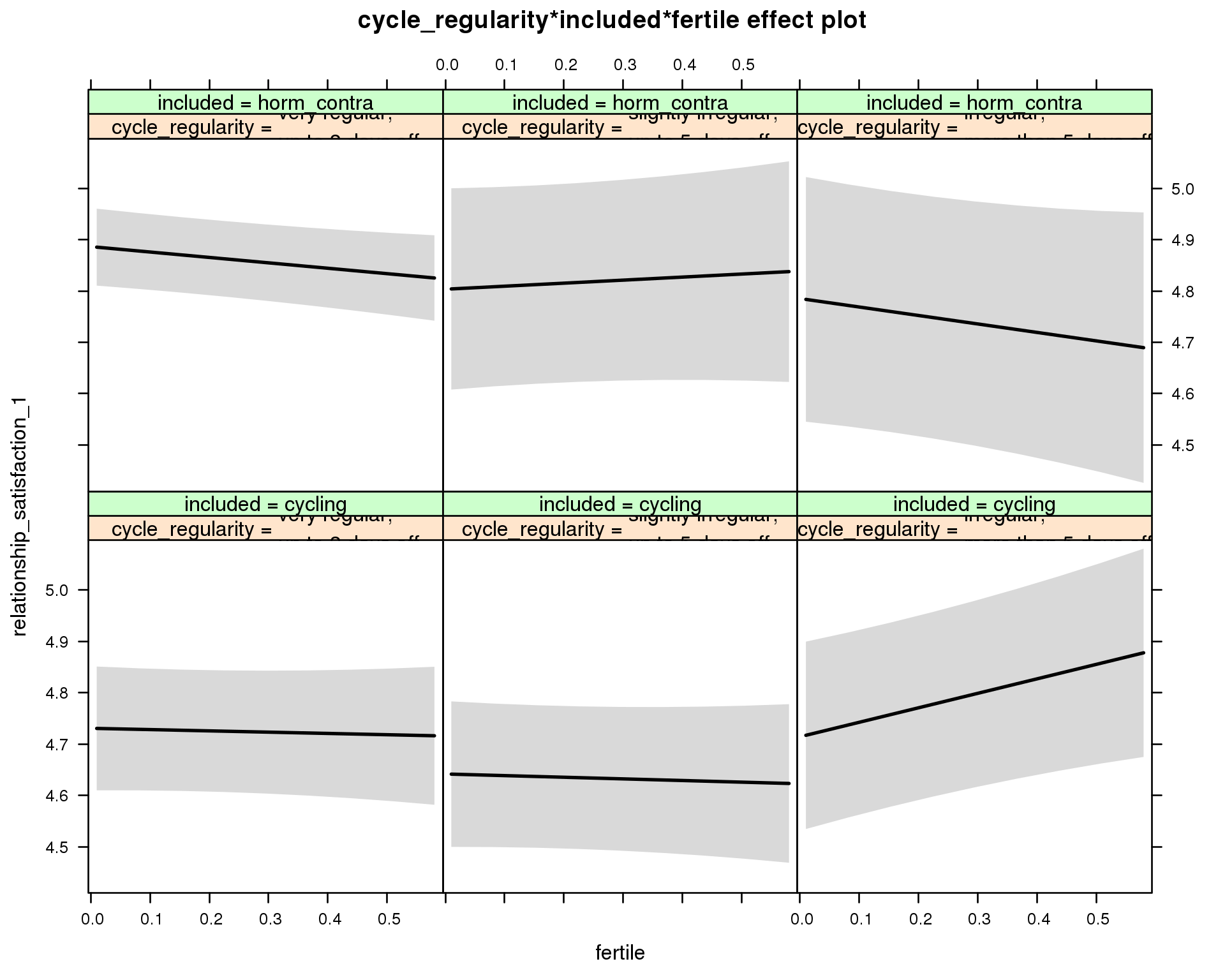
Linear mixed model fit by REML ['lmerMod']
Formula: relationship_satisfaction_1 ~ menstruation + fertile_mean + (1 |
person) + cycle_regularity + included + fertile + menstruation:included +
cycle_regularity:included + cycle_regularity:fertile + included:fertile +
cycle_regularity:included:fertile
Data: diary
REML criterion at convergence: 75057
Scaled residuals:
Min 1Q Median 3Q Max
-4.877 -0.496 0.149 0.647 3.835
Random effects:
Groups Name Variance Std.Dev.
person (Intercept) 0.637 0.798
Residual 0.872 0.934
Number of obs: 26704, groups: person, 1054
Fixed effects:
Estimate Std. Error t value
(Intercept) 4.80460 0.08157 58.9
menstruationpre 0.01941 0.02853 0.7
menstruationyes 0.02209 0.02687 0.8
fertile_mean -0.46770 0.31779 -1.5
cycle_regularityslightly irregular,\nup to 5 days off -0.08899 0.09495 -0.9
cycle_regularityirregular,\nmore than 5 days off -0.01644 0.11158 -0.1
includedhorm_contra 0.16233 0.07436 2.2
fertile -0.02499 0.07967 -0.3
menstruationpre:includedhorm_contra -0.03447 0.03661 -0.9
menstruationyes:includedhorm_contra -0.00247 0.03522 -0.1
cycle_regularityslightly irregular,\nup to 5 days off:includedhorm_contra 0.00597 0.14346 0.0
cycle_regularityirregular,\nmore than 5 days off:includedhorm_contra -0.08474 0.16956 -0.5
cycle_regularityslightly irregular,\nup to 5 days off:fertile -0.00682 0.10990 -0.1
cycle_regularityirregular,\nmore than 5 days off:fertile 0.30695 0.13516 2.3
includedhorm_contra:fertile -0.08037 0.09334 -0.9
cycle_regularityslightly irregular,\nup to 5 days off:includedhorm_contra:fertile 0.17135 0.16315 1.1
cycle_regularityirregular,\nmore than 5 days off:includedhorm_contra:fertile -0.36656 0.20157 -1.8
M_m9: Moderation by cohabitation status
model %>%
test_moderator("cohabitation", diary)refitting model(s) with ML (instead of REML)
| Df | AIC | BIC | logLik | deviance | Chisq | Chi Df | Pr(>Chisq) | |
|---|---|---|---|---|---|---|---|---|
| with_main | 15 | 75026 | 75149 | -37498 | 74996 | NA | NA | NA |
| with_mod | 19 | 75025 | 75181 | -37494 | 74987 | 9.168 | 4 | 0.05702 |
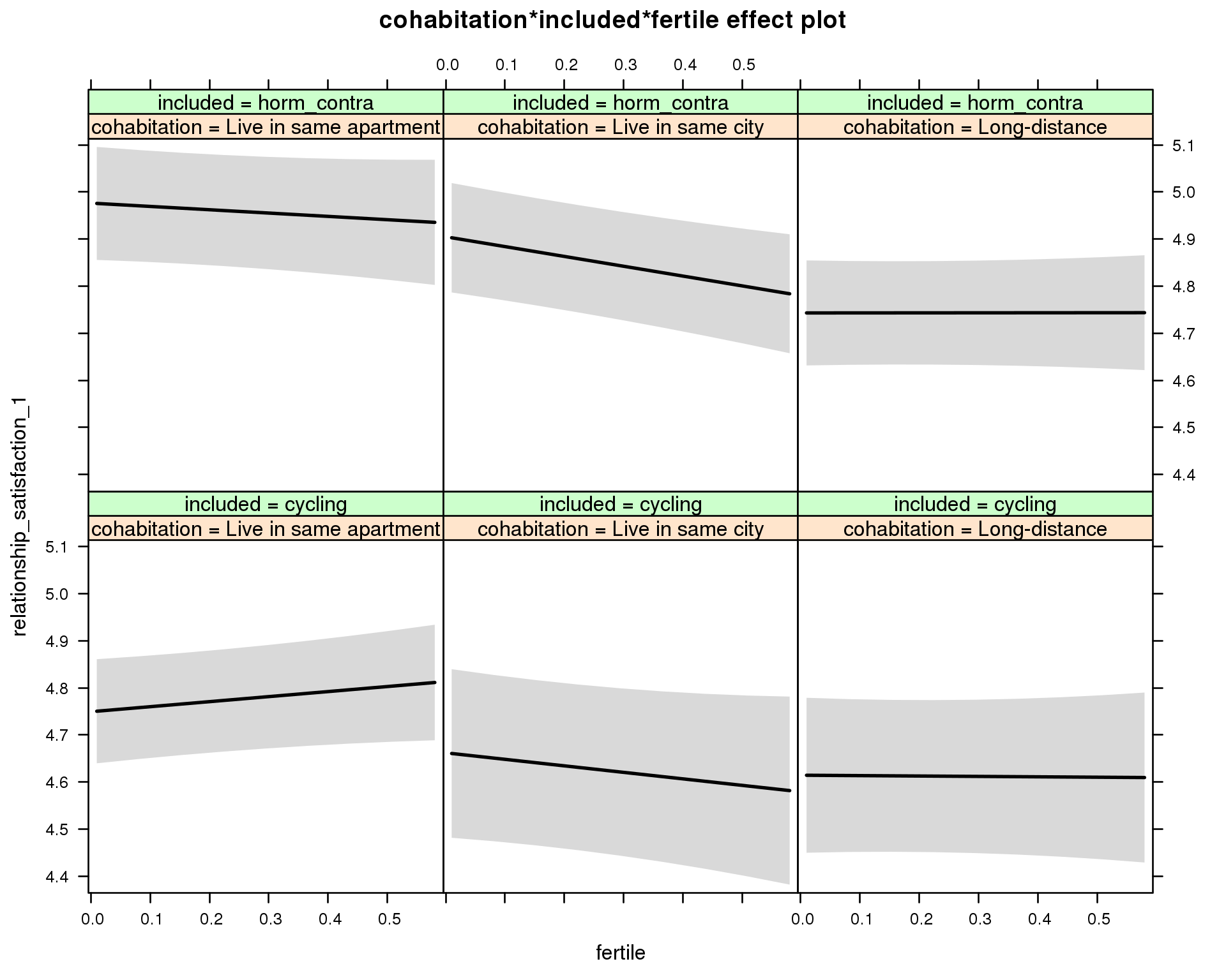
Linear mixed model fit by REML ['lmerMod']
Formula: relationship_satisfaction_1 ~ menstruation + fertile_mean + (1 |
person) + cohabitation + included + fertile + menstruation:included +
cohabitation:included + cohabitation:fertile + included:fertile + cohabitation:included:fertile
Data: diary
REML criterion at convergence: 75051
Scaled residuals:
Min 1Q Median 3Q Max
-4.851 -0.496 0.154 0.647 3.823
Random effects:
Groups Name Variance Std.Dev.
person (Intercept) 0.631 0.794
Residual 0.872 0.934
Number of obs: 26704, groups: person, 1054
Fixed effects:
Estimate Std. Error t value
(Intercept) 4.82301 0.07875 61.2
menstruationpre 0.02189 0.02850 0.8
menstruationyes 0.02397 0.02686 0.9
fertile_mean -0.47032 0.31576 -1.5
cohabitationLive in same city -0.08729 0.10731 -0.8
cohabitationLong-distance -0.13481 0.10111 -1.3
includedhorm_contra 0.23417 0.08476 2.8
fertile 0.10700 0.07193 1.5
menstruationpre:includedhorm_contra -0.03632 0.03660 -1.0
menstruationyes:includedhorm_contra -0.00429 0.03520 -0.1
cohabitationLive in same city:includedhorm_contra 0.01578 0.13713 0.1
cohabitationLong-distance:includedhorm_contra -0.09837 0.13122 -0.7
cohabitationLive in same city:fertile -0.24520 0.13142 -1.9
cohabitationLong-distance:fertile -0.11545 0.11839 -1.0
includedhorm_contra:fertile -0.17746 0.10509 -1.7
cohabitationLive in same city:includedhorm_contra:fertile 0.10705 0.16431 0.7
cohabitationLong-distance:includedhorm_contra:fertile 0.18681 0.15247 1.2
M_m10: Moderation by relationship status
model %>%
test_moderator("relationship_status_clean", diary)refitting model(s) with ML (instead of REML)
| Df | AIC | BIC | logLik | deviance | Chisq | Chi Df | Pr(>Chisq) | |
|---|---|---|---|---|---|---|---|---|
| with_main | 15 | 75033 | 75156 | -37502 | 75003 | NA | NA | NA |
| with_mod | 19 | 75040 | 75195 | -37501 | 75002 | 1.421 | 4 | 0.8405 |
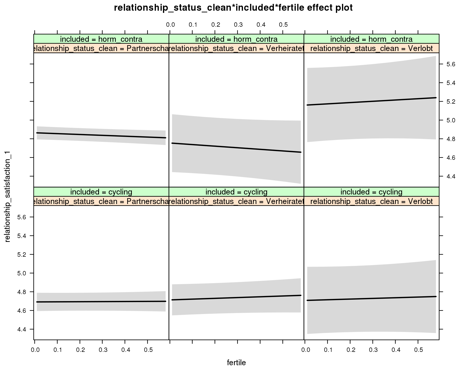
Linear mixed model fit by REML ['lmerMod']
Formula: relationship_satisfaction_1 ~ menstruation + fertile_mean + (1 |
person) + relationship_status_clean + included + fertile +
menstruation:included + relationship_status_clean:included +
relationship_status_clean:fertile + included:fertile + relationship_status_clean:included:fertile
Data: diary
REML criterion at convergence: 75057
Scaled residuals:
Min 1Q Median 3Q Max
-4.873 -0.496 0.151 0.648 3.836
Random effects:
Groups Name Variance Std.Dev.
person (Intercept) 0.635 0.797
Residual 0.872 0.934
Number of obs: 26704, groups: person, 1054
Fixed effects:
Estimate Std. Error t value
(Intercept) 4.76091 0.07390 64.4
menstruationpre 0.02181 0.02851 0.8
menstruationyes 0.02393 0.02686 0.9
fertile_mean -0.44661 0.31625 -1.4
relationship_status_cleanVerheiratet 0.02142 0.09829 0.2
relationship_status_cleanVerlobt 0.01606 0.18999 0.1
includedhorm_contra 0.18130 0.06339 2.9
fertile 0.01120 0.06590 0.2
menstruationpre:includedhorm_contra -0.03731 0.03660 -1.0
menstruationyes:includedhorm_contra -0.00469 0.03520 -0.1
relationship_status_cleanVerheiratet:includedhorm_contra -0.13083 0.18956 -0.7
relationship_status_cleanVerlobt:includedhorm_contra 0.27917 0.28010 1.0
relationship_status_cleanVerheiratet:fertile 0.07276 0.11601 0.6
relationship_status_cleanVerlobt:fertile 0.06052 0.21759 0.3
includedhorm_contra:fertile -0.10350 0.08033 -1.3
relationship_status_cleanVerheiratet:includedhorm_contra:fertile -0.14995 0.21847 -0.7
relationship_status_cleanVerlobt:includedhorm_contra:fertile 0.16912 0.33791 0.5
Communicaton with partner
model_summaries$communication_partner_1Model summary
Model summary
model %>%
print_summary()Linear mixed model fit by REML
t-tests use Satterthwaite approximations to degrees of freedom ['lmerMod']
Formula: communication_partner_1 ~ included * (menstruation + fertile) + fertile_mean + (1 | person)
Data: diary
REML criterion at convergence: 40847
Scaled residuals:
Min 1Q Median 3Q Max
-3.736 -0.849 0.248 0.786 2.917
Random effects:
Groups Name Variance Std.Dev.
person (Intercept) 0.0667 0.258
Residual 0.2505 0.501
Number of obs: 26704, groups: person, 1054
Fixed effects:
Estimate Std. Error df t value Pr(>|t|)
(Intercept) 2.54706 0.02571 1640.00000 99.09 <2e-16 ***
includedhorm_contra 0.04013 0.02108 1759.00000 1.90 0.057 .
menstruationpre 0.01814 0.01521 26265.00000 1.19 0.233
menstruationyes 0.00679 0.01431 26407.00000 0.47 0.635
fertile -0.02078 0.03072 26215.00000 -0.68 0.499
fertile_mean -0.10568 0.11924 1714.00000 -0.89 0.376
includedhorm_contra:menstruationpre -0.04980 0.01953 26267.00000 -2.55 0.011 *
includedhorm_contra:menstruationyes -0.02767 0.01876 26375.00000 -1.47 0.140
includedhorm_contra:fertile -0.04134 0.03884 26386.00000 -1.06 0.287
---
Signif. codes: 0 '***' 0.001 '**' 0.01 '*' 0.05 '.' 0.1 ' ' 1
Correlation of Fixed Effects:
(Intr) incld_ mnstrtnp mnstrtny fertil frtl_m inclddhrm_cntr:mnstrtnp
inclddhrm_c -0.476
menstrutnpr -0.233 0.291
menstrutnys -0.225 0.278 0.394
fertile -0.221 0.356 0.466 0.383
fertile_men -0.769 -0.030 -0.006 -0.004 -0.089
inclddhrm_cntr:mnstrtnp 0.191 -0.364 -0.779 -0.307 -0.362 -0.007
inclddhrm_cntr:mnstrtny 0.179 -0.341 -0.301 -0.763 -0.291 -0.007 0.380
inclddhrm_cntr:f 0.221 -0.451 -0.368 -0.303 -0.785 0.011 0.466
inclddhrm_cntr:mnstrtny
inclddhrm_c
menstrutnpr
menstrutnys
fertile
fertile_men
inclddhrm_cntr:mnstrtnp
inclddhrm_cntr:mnstrtny
inclddhrm_cntr:f 0.380
Effect size standardised by residual variance (\(\frac{b}{ SD_{residual} }\)): -0.04 [-0.16;0.08].
Marginal effect plots
model %>%
plot_all_effects()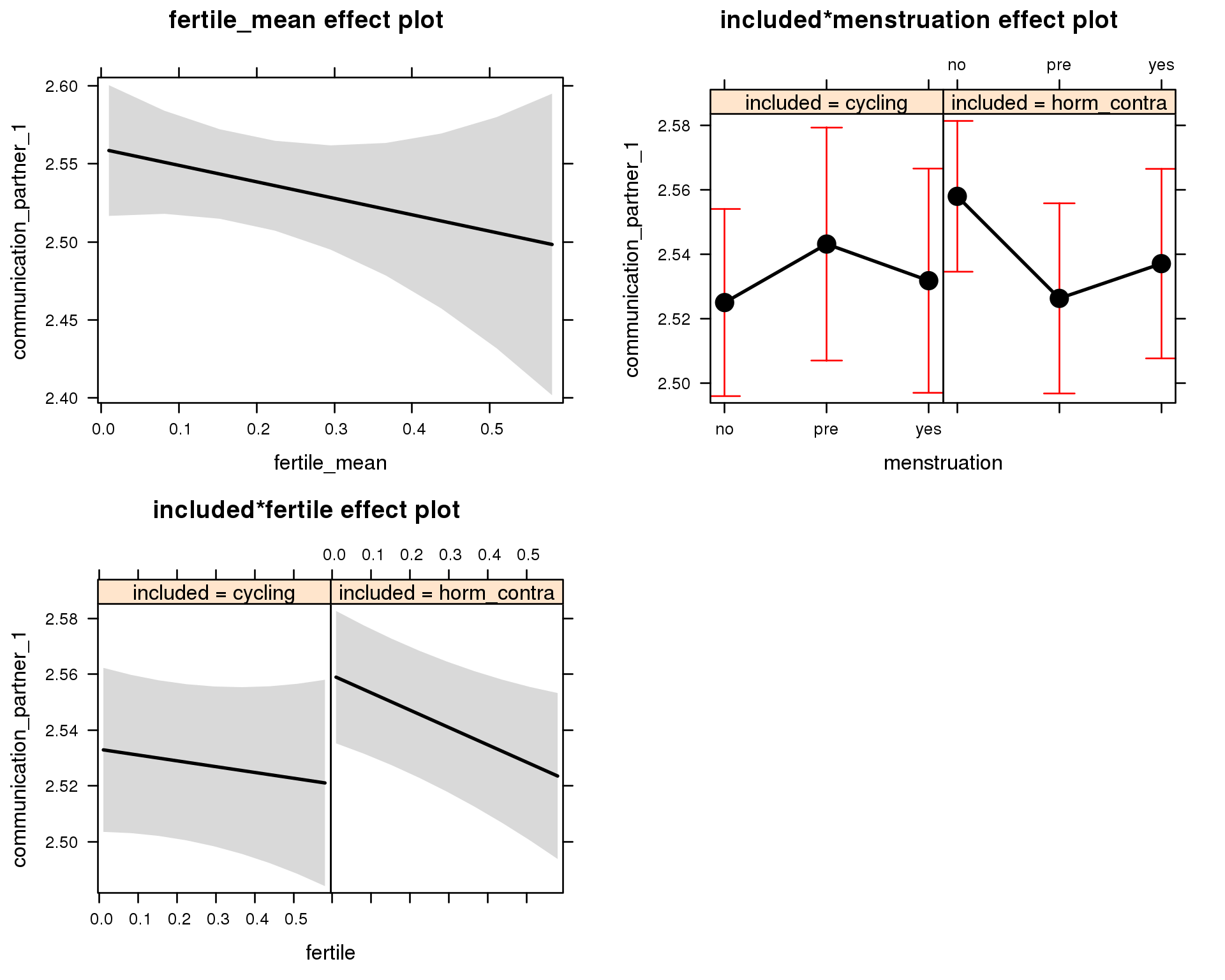
Outcome distribution
model %>%
plot_outcome(diary) + xlab(outcome_label)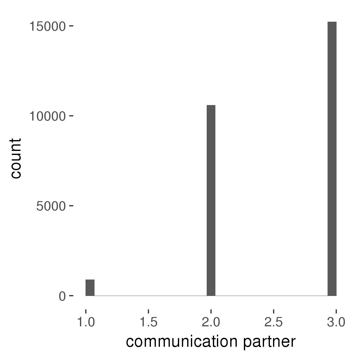
Diagnostics
model %>%
print_diagnostics()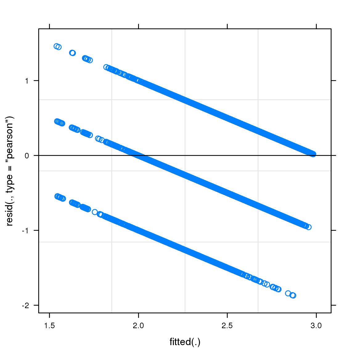
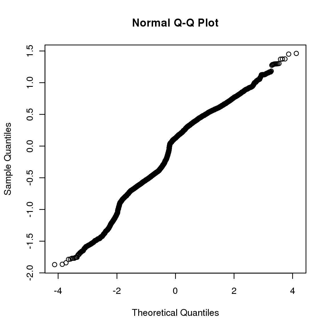
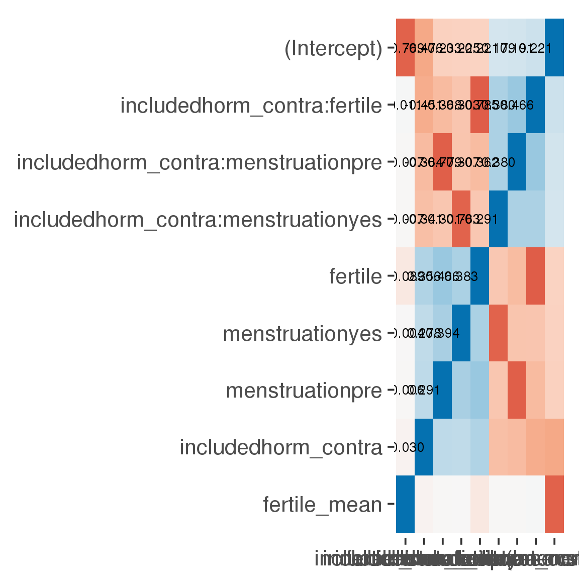
Curves
Here, we continuously plot the outcome over the course of the cycle. Because cycle lengths vary, we subset the data to cycles in a certain range. If the red curve traces the pink curve, our predictor accurately maps the relationship between fertile window probability and the outcome.
Cycle lengths from 21 to 36
Backward-counted
model %>%
plot_curve(diary %>% filter(minimum_cycle_length_diary <= 36, minimum_cycle_length_diary > 20) %>% mutate(fertile=prc_stirn_b))outcome = names(model@frame)[1]
outcome_label = recode(str_replace_all(str_replace_all(str_replace_all(outcome, "_", " "), " pair", "-pair"), " 1", ""),
"desirability 1" = "self-perceived desirability",
"NARQ admiration" = "narcissistic admiration",
"NARQ rivalry" = "narcissistic rivalry",
"extra-pair" = "extra-pair desire & behaviour",
"had sexual intercourse" = "sexual intercourse")
library(ggplot2)
# form a subset and run the model without the hormonal contraception and the fertility predictors
tmp = diary %>%
filter(!is.na(fertile), !is.na(included),
RCD > -1 * minimum_cycle_length_diary, RCD > -40)
new_form = update.formula(formula(model), new = . ~ . - fertile * included)
tmp$residuals = residuals(update(model, new_form, data = tmp , na.action = na.exclude))
tmp = tmp %>%
filter(!is.na(RCD), !is.na(residuals))
rcd_min = min(tmp$RCD)
tmp$real = FALSE
tmp_before = tmp
tmp_before$RCD = tmp_before$RCD + min(tmp$RCD) - 1
tmp_after = tmp
tmp_after$RCD = tmp_after$RCD - min(tmp$RCD) + 1
tmp$real = TRUE
tmp = bind_rows(tmp_before %>% filter(RCD > rcd_min - 11), tmp, tmp_after %>% filter(RCD < 11))GAM smooth on residuals
Here, we partialled out menstruation and individual random effects, then superimposed estimated probability of being in the fertile window scaled to the range of the estimated means. To address the periodicity of the cycle, we prepended and appended ten days of the timeseries to the end and the beginning of the timeseries. We then estimated the GAM and cut off the appended subsets before plotting.
tryCatch({
trend_plot = ggplot(tmp,aes(x = RCD, y = residuals, colour = included)) +
stat_smooth(geom = 'smooth',size = 0.8, fill = "#9ECAE1", method = 'gam', formula = y ~ s(x))
}, error = function(e){cat_message(e, "danger")})
tryCatch({
trend_data = ggplot_build(trend_plot)$data[[1]]
}, error = function(e){cat_message(e, "danger")})
trend_data$RCD = round(trend_data$x)
trend_data = left_join(trend_data, tmp %>% select(real, RCD,fertile) %>% unique(), by = "RCD")
trend_data %>%
filter(real == TRUE) %>%
mutate(superimposed = ( ( (fertile - 0.01)/0.58) * (max(y)-min(y) ) ) + min(y) ) ->
trend_data
ggplot(trend_data) +
geom_ribbon(aes(x = x, ymin = ymin, ymax = ymax, fill = factor(group)), alpha = 0.2) +
geom_line(aes(x = x, y = y, colour = factor(group)), size = 0.8, stat = "identity") +
scale_x_continuous(caption_x) +
geom_line(aes(x = x, y = superimposed), color = "#a83fbf", size = 1, linetype = 'dashed') +
annotate("text",x = mean(trend_data$x), y = max(trend_data$superimposed,na.rm=T) + 0.1, label = 'superimposed fertility peak', color = "#a83fbf") +
scale_y_continuous(outcome_label) +
ggtitle("GAM smooth, residuals") +
scale_color_manual("Contraception status",values = c("2"="black","1"= "red"), labels = c("2"="hormonally\ncontracepting","1"="cycling"), guide = F) +
scale_fill_manual("Contraception status",values = c("2"="black","1"= "red"), labels = c("2"="hormonally\ncontracepting","1"="cycling"), guide = F)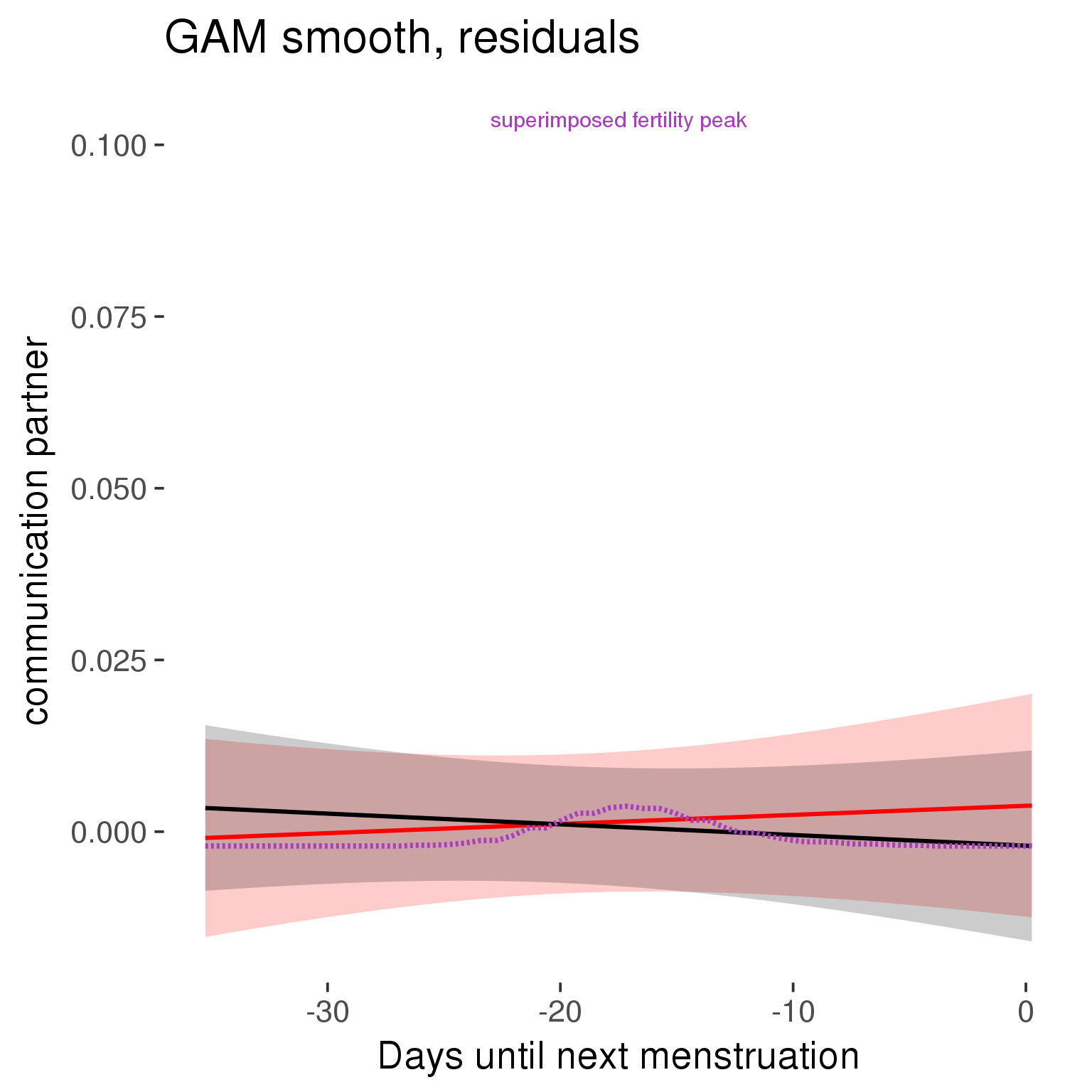
GAM smooth on raw data
As before, but without partialling anything out.
tryCatch({
trend_plot = ggplot(tmp,aes_string(x = "RCD", y = outcome, colour = "included")) +
stat_smooth(geom = 'smooth',size = 0.8, fill = "#9ECAE1", method = 'gam', formula = y ~ s(x))
}, error = function(e){cat_message(e, "danger")})
tryCatch({
trend_data = ggplot_build(trend_plot)$data[[1]]
}, error = function(e){cat_message(e, "danger")})
trend_data$RCD = round(trend_data$x)
trend_data = left_join(trend_data, tmp %>% select(real, RCD,fertile) %>% unique(), by = "RCD")
trend_data %>%
filter(real == TRUE) %>%
mutate(superimposed = ( ( (fertile - 0.01)/0.58) * (max(y)-min(y) ) ) + min(y) ) ->
trend_data
plot1b = ggplot(trend_data) +
geom_ribbon(aes(x = x, ymin = ymin, ymax = ymax, fill = factor(group)), alpha = 0.2) +
geom_line(aes(x = x, y = y, colour = factor(group)), size = 0.8, stat = "identity") +
scale_x_continuous(caption_x) +
geom_line(aes(x = x, y = superimposed), color = "#a83fbf", size = 1, linetype = 'dashed') +
annotate("text",x = mean(trend_data$x), y = max(trend_data$superimposed,na.rm=T) + 0.1, label = 'superimposed fertility peak', color = "#a83fbf") +
scale_y_continuous(outcome_label) +
ggtitle("GAM smooth, raw data") +
scale_color_manual("Contraception status",values = c("2"="black","1"= "red"), labels = c("2"="hormonally\ncontracepting","1"="cycling"), guide = F) +
scale_fill_manual("Contraception status",values = c("2"="black","1"= "red"), labels = c("2"="hormonally\ncontracepting","1"="cycling"), guide = F)
suppressWarnings(print(plot1b))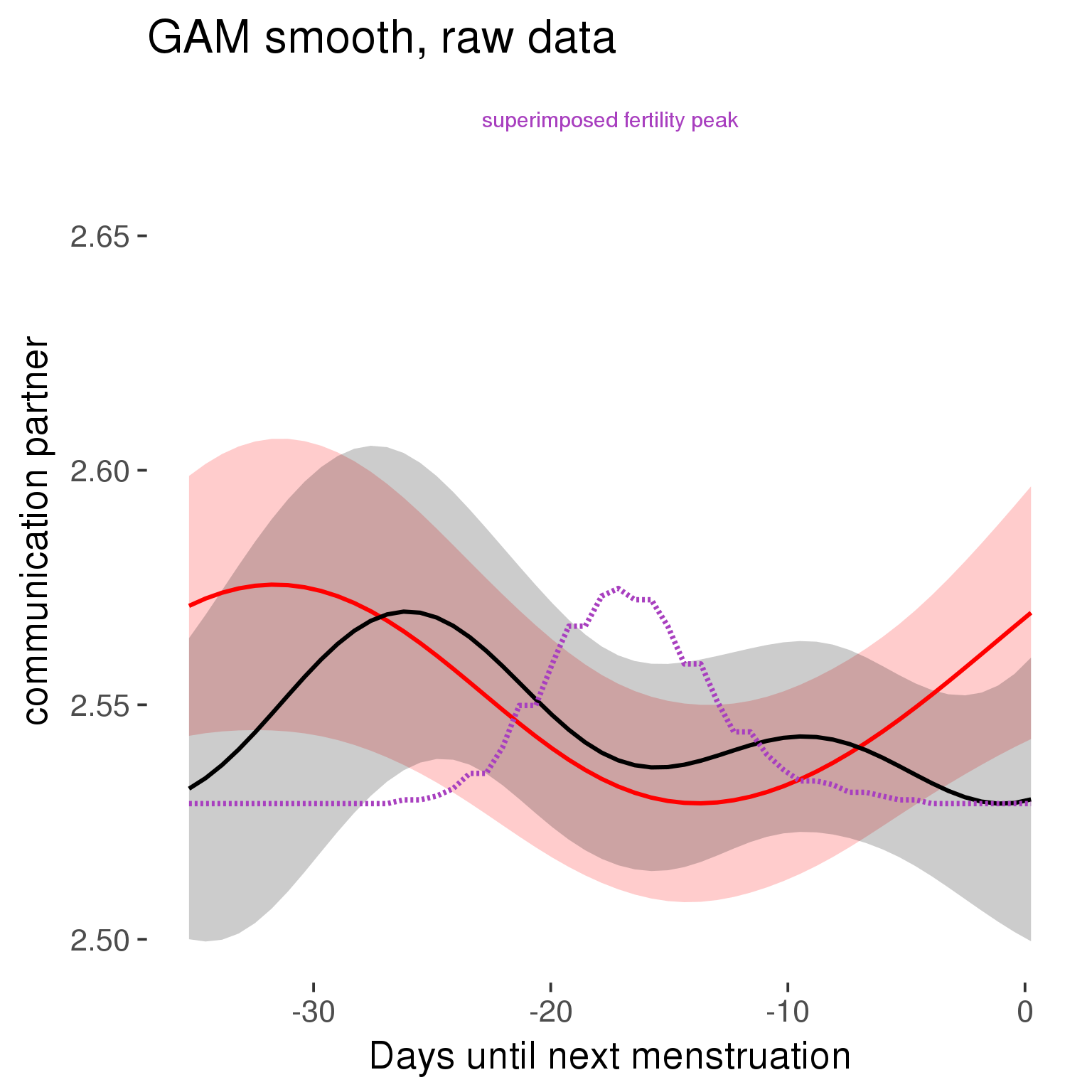
Means and standard errors over raw data
Nothing partialled out, just straight means with bootstrapped confidence intervals.
tryCatch({
trend_plot = ggplot(tmp,aes_string(x = "RCD", y = outcome, colour = "included")) +
geom_pointrange(size = 0.8, stat = 'summary', fun.data = "mean_cl_boot")
}, error = function(e){cat_message(e, "danger")})
tryCatch({
trend_data = ggplot_build(trend_plot)$data[[1]]
}, error = function(e){cat_message(e, "danger")})
trend_data$RCD = round(trend_data$x)
trend_data = left_join(trend_data, tmp %>% select(real, RCD,fertile) %>% unique(), by = "RCD")
trend_data %>%
filter(real == TRUE) %>%
mutate(superimposed = ( ( (fertile - 0.01)/0.58) * (max(y)-min(y) ) ) + min(y) ) ->
trend_data
plot3 = ggplot(trend_data) +
geom_pointrange(aes(x = x, y = y, ymin = ymin,ymax = ymax, colour = factor(group)), size = 0.8, stat = "identity", alpha = 0.6, position = position_dodge(width = .5)) +
scale_x_continuous("Days until next menstruation") +
geom_line(aes(x= x, y = superimposed), color = "#a83fbf", size = 1, linetype = 'dashed') +
annotate("text",x = mean(trend_data$x), y = max(trend_data$superimposed,na.rm=T) + 0.1, label = 'superimposed fertility peak', color = "#a83fbf") +
scale_y_continuous(outcome_label) +
ggtitle("Means with standard errors, raw data") +
scale_color_manual("Contraception status",values = c("2"="black","1"= "red"), labels = c("2"="hormonally\ncontracepting","1"="cycling"), guide = F) +
scale_fill_manual("Contraception status",values = c("2"="black","1"= "red"), labels = c("2"="hormonally\ncontracepting","1"="cycling"), guide = F)
suppressWarnings(print(plot3))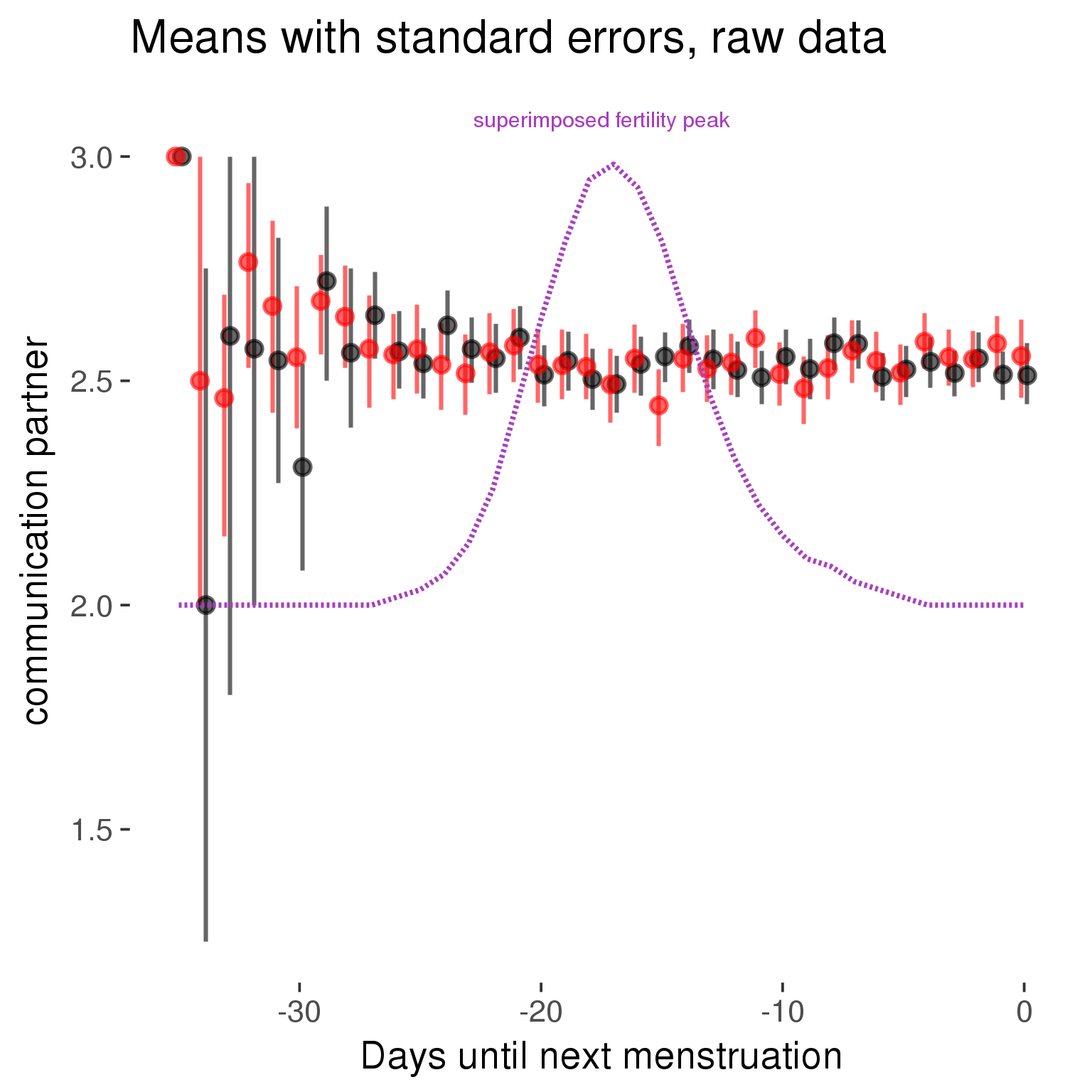
Forward-counted
model %>%
plot_curve(diary %>% filter(minimum_cycle_length_diary <= 36, minimum_cycle_length_diary > 20) %>% mutate(RCD = FCD, fertile = prc_stirn_b_forward_counted), caption_x = "Days since last menstruation")outcome = names(model@frame)[1]
outcome_label = recode(str_replace_all(str_replace_all(str_replace_all(outcome, "_", " "), " pair", "-pair"), " 1", ""),
"desirability 1" = "self-perceived desirability",
"NARQ admiration" = "narcissistic admiration",
"NARQ rivalry" = "narcissistic rivalry",
"extra-pair" = "extra-pair desire & behaviour",
"had sexual intercourse" = "sexual intercourse")
library(ggplot2)
# form a subset and run the model without the hormonal contraception and the fertility predictors
tmp = diary %>%
filter(!is.na(fertile), !is.na(included),
RCD > -1 * minimum_cycle_length_diary, RCD > -40)
new_form = update.formula(formula(model), new = . ~ . - fertile * included)
tmp$residuals = residuals(update(model, new_form, data = tmp , na.action = na.exclude))
tmp = tmp %>%
filter(!is.na(RCD), !is.na(residuals))
rcd_min = min(tmp$RCD)
tmp$real = FALSE
tmp_before = tmp
tmp_before$RCD = tmp_before$RCD + min(tmp$RCD) - 1
tmp_after = tmp
tmp_after$RCD = tmp_after$RCD - min(tmp$RCD) + 1
tmp$real = TRUE
tmp = bind_rows(tmp_before %>% filter(RCD > rcd_min - 11), tmp, tmp_after %>% filter(RCD < 11))GAM smooth on residuals
Here, we partialled out menstruation and individual random effects, then superimposed estimated probability of being in the fertile window scaled to the range of the estimated means. To address the periodicity of the cycle, we prepended and appended ten days of the timeseries to the end and the beginning of the timeseries. We then estimated the GAM and cut off the appended subsets before plotting.
tryCatch({
trend_plot = ggplot(tmp,aes(x = RCD, y = residuals, colour = included)) +
stat_smooth(geom = 'smooth',size = 0.8, fill = "#9ECAE1", method = 'gam', formula = y ~ s(x))
}, error = function(e){cat_message(e, "danger")})
tryCatch({
trend_data = ggplot_build(trend_plot)$data[[1]]
}, error = function(e){cat_message(e, "danger")})
trend_data$RCD = round(trend_data$x)
trend_data = left_join(trend_data, tmp %>% select(real, RCD,fertile) %>% unique(), by = "RCD")
trend_data %>%
filter(real == TRUE) %>%
mutate(superimposed = ( ( (fertile - 0.01)/0.58) * (max(y)-min(y) ) ) + min(y) ) ->
trend_data
ggplot(trend_data) +
geom_ribbon(aes(x = x, ymin = ymin, ymax = ymax, fill = factor(group)), alpha = 0.2) +
geom_line(aes(x = x, y = y, colour = factor(group)), size = 0.8, stat = "identity") +
scale_x_continuous(caption_x) +
geom_line(aes(x = x, y = superimposed), color = "#a83fbf", size = 1, linetype = 'dashed') +
annotate("text",x = mean(trend_data$x), y = max(trend_data$superimposed,na.rm=T) + 0.1, label = 'superimposed fertility peak', color = "#a83fbf") +
scale_y_continuous(outcome_label) +
ggtitle("GAM smooth, residuals") +
scale_color_manual("Contraception status",values = c("2"="black","1"= "red"), labels = c("2"="hormonally\ncontracepting","1"="cycling"), guide = F) +
scale_fill_manual("Contraception status",values = c("2"="black","1"= "red"), labels = c("2"="hormonally\ncontracepting","1"="cycling"), guide = F)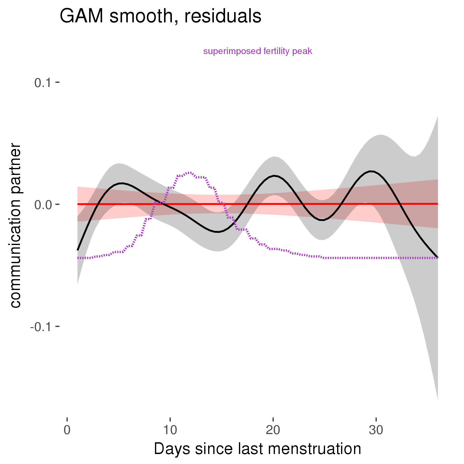
GAM smooth on raw data
As before, but without partialling anything out.
tryCatch({
trend_plot = ggplot(tmp,aes_string(x = "RCD", y = outcome, colour = "included")) +
stat_smooth(geom = 'smooth',size = 0.8, fill = "#9ECAE1", method = 'gam', formula = y ~ s(x))
}, error = function(e){cat_message(e, "danger")})
tryCatch({
trend_data = ggplot_build(trend_plot)$data[[1]]
}, error = function(e){cat_message(e, "danger")})
trend_data$RCD = round(trend_data$x)
trend_data = left_join(trend_data, tmp %>% select(real, RCD,fertile) %>% unique(), by = "RCD")
trend_data %>%
filter(real == TRUE) %>%
mutate(superimposed = ( ( (fertile - 0.01)/0.58) * (max(y)-min(y) ) ) + min(y) ) ->
trend_data
plot1b = ggplot(trend_data) +
geom_ribbon(aes(x = x, ymin = ymin, ymax = ymax, fill = factor(group)), alpha = 0.2) +
geom_line(aes(x = x, y = y, colour = factor(group)), size = 0.8, stat = "identity") +
scale_x_continuous(caption_x) +
geom_line(aes(x = x, y = superimposed), color = "#a83fbf", size = 1, linetype = 'dashed') +
annotate("text",x = mean(trend_data$x), y = max(trend_data$superimposed,na.rm=T) + 0.1, label = 'superimposed fertility peak', color = "#a83fbf") +
scale_y_continuous(outcome_label) +
ggtitle("GAM smooth, raw data") +
scale_color_manual("Contraception status",values = c("2"="black","1"= "red"), labels = c("2"="hormonally\ncontracepting","1"="cycling"), guide = F) +
scale_fill_manual("Contraception status",values = c("2"="black","1"= "red"), labels = c("2"="hormonally\ncontracepting","1"="cycling"), guide = F)
suppressWarnings(print(plot1b))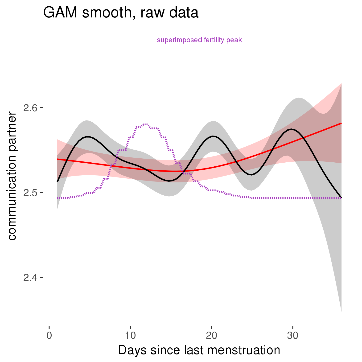
Means and standard errors over raw data
Nothing partialled out, just straight means with bootstrapped confidence intervals.
tryCatch({
trend_plot = ggplot(tmp,aes_string(x = "RCD", y = outcome, colour = "included")) +
geom_pointrange(size = 0.8, stat = 'summary', fun.data = "mean_cl_boot")
}, error = function(e){cat_message(e, "danger")})
tryCatch({
trend_data = ggplot_build(trend_plot)$data[[1]]
}, error = function(e){cat_message(e, "danger")})
trend_data$RCD = round(trend_data$x)
trend_data = left_join(trend_data, tmp %>% select(real, RCD,fertile) %>% unique(), by = "RCD")
trend_data %>%
filter(real == TRUE) %>%
mutate(superimposed = ( ( (fertile - 0.01)/0.58) * (max(y)-min(y) ) ) + min(y) ) ->
trend_data
plot3 = ggplot(trend_data) +
geom_pointrange(aes(x = x, y = y, ymin = ymin,ymax = ymax, colour = factor(group)), size = 0.8, stat = "identity", alpha = 0.6, position = position_dodge(width = .5)) +
scale_x_continuous("Days until next menstruation") +
geom_line(aes(x= x, y = superimposed), color = "#a83fbf", size = 1, linetype = 'dashed') +
annotate("text",x = mean(trend_data$x), y = max(trend_data$superimposed,na.rm=T) + 0.1, label = 'superimposed fertility peak', color = "#a83fbf") +
scale_y_continuous(outcome_label) +
ggtitle("Means with standard errors, raw data") +
scale_color_manual("Contraception status",values = c("2"="black","1"= "red"), labels = c("2"="hormonally\ncontracepting","1"="cycling"), guide = F) +
scale_fill_manual("Contraception status",values = c("2"="black","1"= "red"), labels = c("2"="hormonally\ncontracepting","1"="cycling"), guide = F)
suppressWarnings(print(plot3))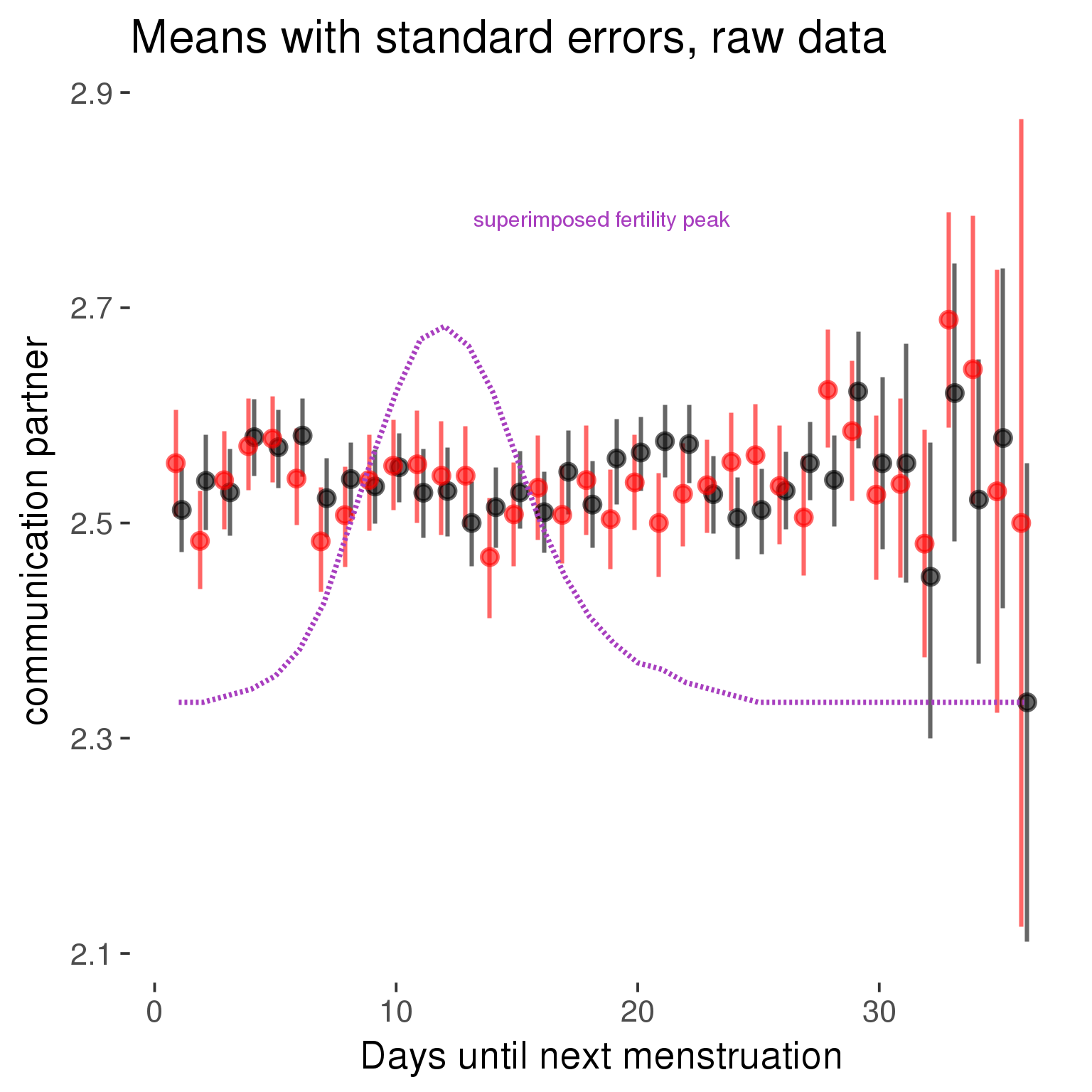
Cycle lengths from 27 to 30
Backward-counted
model %>%
plot_curve(diary %>% filter(minimum_cycle_length_diary <= 30, minimum_cycle_length_diary >= 27) %>% mutate(fertile=prc_stirn_b))outcome = names(model@frame)[1]
outcome_label = recode(str_replace_all(str_replace_all(str_replace_all(outcome, "_", " "), " pair", "-pair"), " 1", ""),
"desirability 1" = "self-perceived desirability",
"NARQ admiration" = "narcissistic admiration",
"NARQ rivalry" = "narcissistic rivalry",
"extra-pair" = "extra-pair desire & behaviour",
"had sexual intercourse" = "sexual intercourse")
library(ggplot2)
# form a subset and run the model without the hormonal contraception and the fertility predictors
tmp = diary %>%
filter(!is.na(fertile), !is.na(included),
RCD > -1 * minimum_cycle_length_diary, RCD > -40)
new_form = update.formula(formula(model), new = . ~ . - fertile * included)
tmp$residuals = residuals(update(model, new_form, data = tmp , na.action = na.exclude))
tmp = tmp %>%
filter(!is.na(RCD), !is.na(residuals))
rcd_min = min(tmp$RCD)
tmp$real = FALSE
tmp_before = tmp
tmp_before$RCD = tmp_before$RCD + min(tmp$RCD) - 1
tmp_after = tmp
tmp_after$RCD = tmp_after$RCD - min(tmp$RCD) + 1
tmp$real = TRUE
tmp = bind_rows(tmp_before %>% filter(RCD > rcd_min - 11), tmp, tmp_after %>% filter(RCD < 11))GAM smooth on residuals
Here, we partialled out menstruation and individual random effects, then superimposed estimated probability of being in the fertile window scaled to the range of the estimated means. To address the periodicity of the cycle, we prepended and appended ten days of the timeseries to the end and the beginning of the timeseries. We then estimated the GAM and cut off the appended subsets before plotting.
tryCatch({
trend_plot = ggplot(tmp,aes(x = RCD, y = residuals, colour = included)) +
stat_smooth(geom = 'smooth',size = 0.8, fill = "#9ECAE1", method = 'gam', formula = y ~ s(x))
}, error = function(e){cat_message(e, "danger")})
tryCatch({
trend_data = ggplot_build(trend_plot)$data[[1]]
}, error = function(e){cat_message(e, "danger")})
trend_data$RCD = round(trend_data$x)
trend_data = left_join(trend_data, tmp %>% select(real, RCD,fertile) %>% unique(), by = "RCD")
trend_data %>%
filter(real == TRUE) %>%
mutate(superimposed = ( ( (fertile - 0.01)/0.58) * (max(y)-min(y) ) ) + min(y) ) ->
trend_data
ggplot(trend_data) +
geom_ribbon(aes(x = x, ymin = ymin, ymax = ymax, fill = factor(group)), alpha = 0.2) +
geom_line(aes(x = x, y = y, colour = factor(group)), size = 0.8, stat = "identity") +
scale_x_continuous(caption_x) +
geom_line(aes(x = x, y = superimposed), color = "#a83fbf", size = 1, linetype = 'dashed') +
annotate("text",x = mean(trend_data$x), y = max(trend_data$superimposed,na.rm=T) + 0.1, label = 'superimposed fertility peak', color = "#a83fbf") +
scale_y_continuous(outcome_label) +
ggtitle("GAM smooth, residuals") +
scale_color_manual("Contraception status",values = c("2"="black","1"= "red"), labels = c("2"="hormonally\ncontracepting","1"="cycling"), guide = F) +
scale_fill_manual("Contraception status",values = c("2"="black","1"= "red"), labels = c("2"="hormonally\ncontracepting","1"="cycling"), guide = F)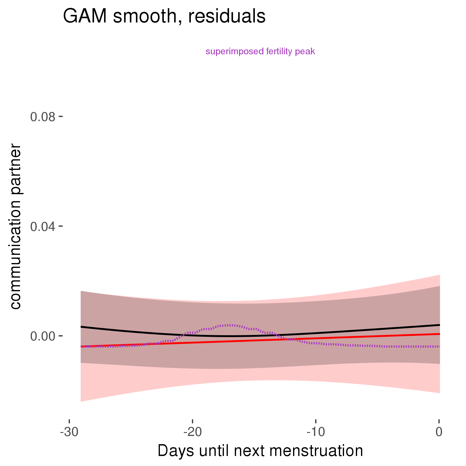
GAM smooth on raw data
As before, but without partialling anything out.
tryCatch({
trend_plot = ggplot(tmp,aes_string(x = "RCD", y = outcome, colour = "included")) +
stat_smooth(geom = 'smooth',size = 0.8, fill = "#9ECAE1", method = 'gam', formula = y ~ s(x))
}, error = function(e){cat_message(e, "danger")})
tryCatch({
trend_data = ggplot_build(trend_plot)$data[[1]]
}, error = function(e){cat_message(e, "danger")})
trend_data$RCD = round(trend_data$x)
trend_data = left_join(trend_data, tmp %>% select(real, RCD,fertile) %>% unique(), by = "RCD")
trend_data %>%
filter(real == TRUE) %>%
mutate(superimposed = ( ( (fertile - 0.01)/0.58) * (max(y)-min(y) ) ) + min(y) ) ->
trend_data
plot1b = ggplot(trend_data) +
geom_ribbon(aes(x = x, ymin = ymin, ymax = ymax, fill = factor(group)), alpha = 0.2) +
geom_line(aes(x = x, y = y, colour = factor(group)), size = 0.8, stat = "identity") +
scale_x_continuous(caption_x) +
geom_line(aes(x = x, y = superimposed), color = "#a83fbf", size = 1, linetype = 'dashed') +
annotate("text",x = mean(trend_data$x), y = max(trend_data$superimposed,na.rm=T) + 0.1, label = 'superimposed fertility peak', color = "#a83fbf") +
scale_y_continuous(outcome_label) +
ggtitle("GAM smooth, raw data") +
scale_color_manual("Contraception status",values = c("2"="black","1"= "red"), labels = c("2"="hormonally\ncontracepting","1"="cycling"), guide = F) +
scale_fill_manual("Contraception status",values = c("2"="black","1"= "red"), labels = c("2"="hormonally\ncontracepting","1"="cycling"), guide = F)
suppressWarnings(print(plot1b))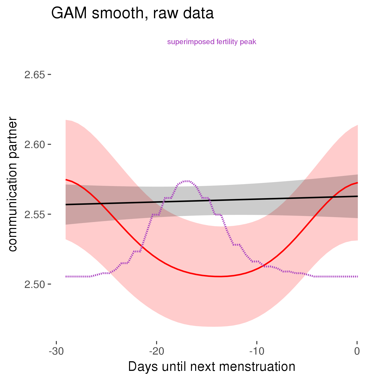
Means and standard errors over raw data
Nothing partialled out, just straight means with bootstrapped confidence intervals.
tryCatch({
trend_plot = ggplot(tmp,aes_string(x = "RCD", y = outcome, colour = "included")) +
geom_pointrange(size = 0.8, stat = 'summary', fun.data = "mean_cl_boot")
}, error = function(e){cat_message(e, "danger")})
tryCatch({
trend_data = ggplot_build(trend_plot)$data[[1]]
}, error = function(e){cat_message(e, "danger")})
trend_data$RCD = round(trend_data$x)
trend_data = left_join(trend_data, tmp %>% select(real, RCD,fertile) %>% unique(), by = "RCD")
trend_data %>%
filter(real == TRUE) %>%
mutate(superimposed = ( ( (fertile - 0.01)/0.58) * (max(y)-min(y) ) ) + min(y) ) ->
trend_data
plot3 = ggplot(trend_data) +
geom_pointrange(aes(x = x, y = y, ymin = ymin,ymax = ymax, colour = factor(group)), size = 0.8, stat = "identity", alpha = 0.6, position = position_dodge(width = .5)) +
scale_x_continuous("Days until next menstruation") +
geom_line(aes(x= x, y = superimposed), color = "#a83fbf", size = 1, linetype = 'dashed') +
annotate("text",x = mean(trend_data$x), y = max(trend_data$superimposed,na.rm=T) + 0.1, label = 'superimposed fertility peak', color = "#a83fbf") +
scale_y_continuous(outcome_label) +
ggtitle("Means with standard errors, raw data") +
scale_color_manual("Contraception status",values = c("2"="black","1"= "red"), labels = c("2"="hormonally\ncontracepting","1"="cycling"), guide = F) +
scale_fill_manual("Contraception status",values = c("2"="black","1"= "red"), labels = c("2"="hormonally\ncontracepting","1"="cycling"), guide = F)
suppressWarnings(print(plot3))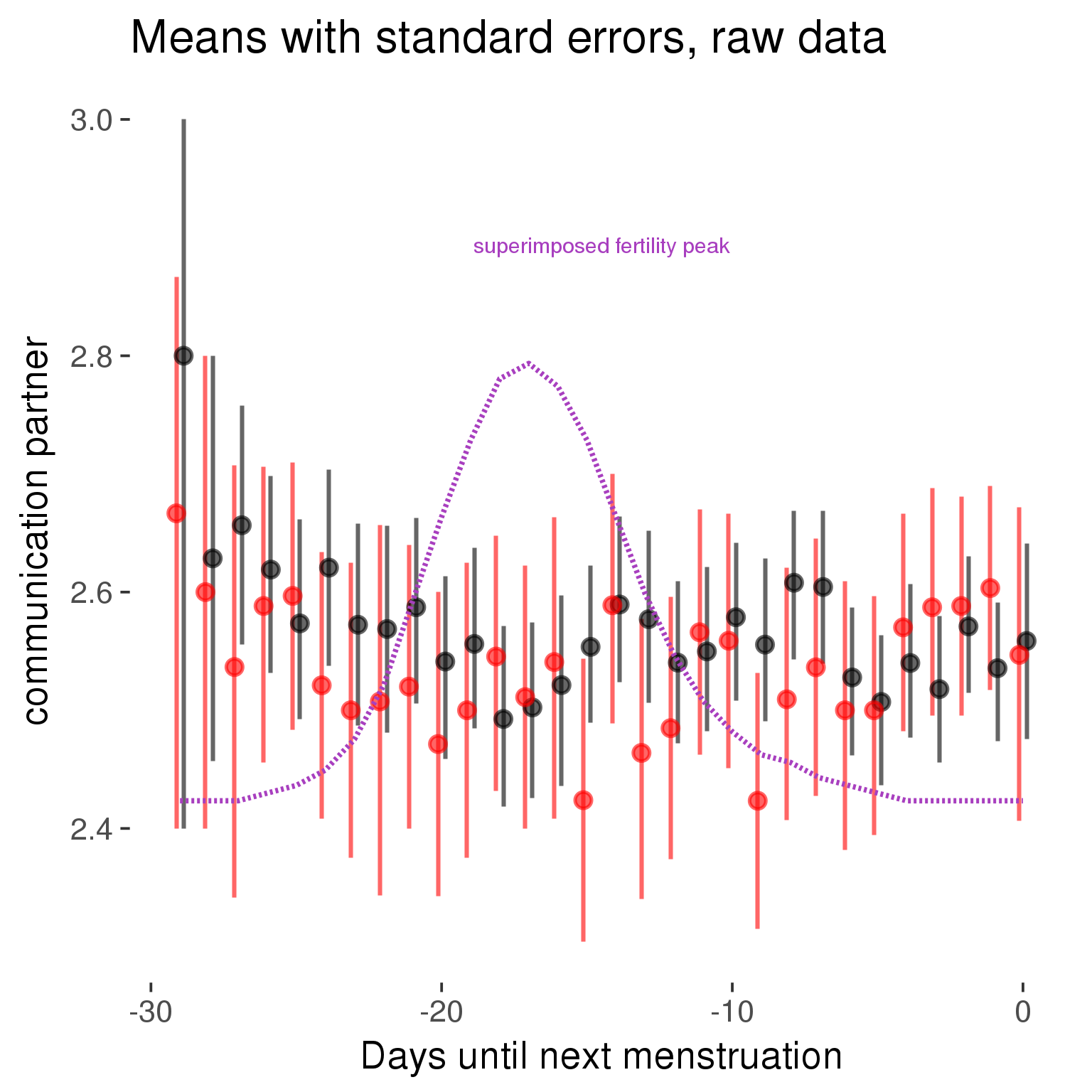
Forward-counted
model %>%
plot_curve(diary %>% filter(minimum_cycle_length_diary <= 30, minimum_cycle_length_diary >= 27) %>% mutate(RCD = FCD, fertile = prc_stirn_b_forward_counted), caption_x = "Days since last menstruation")outcome = names(model@frame)[1]
outcome_label = recode(str_replace_all(str_replace_all(str_replace_all(outcome, "_", " "), " pair", "-pair"), " 1", ""),
"desirability 1" = "self-perceived desirability",
"NARQ admiration" = "narcissistic admiration",
"NARQ rivalry" = "narcissistic rivalry",
"extra-pair" = "extra-pair desire & behaviour",
"had sexual intercourse" = "sexual intercourse")
library(ggplot2)
# form a subset and run the model without the hormonal contraception and the fertility predictors
tmp = diary %>%
filter(!is.na(fertile), !is.na(included),
RCD > -1 * minimum_cycle_length_diary, RCD > -40)
new_form = update.formula(formula(model), new = . ~ . - fertile * included)
tmp$residuals = residuals(update(model, new_form, data = tmp , na.action = na.exclude))
tmp = tmp %>%
filter(!is.na(RCD), !is.na(residuals))
rcd_min = min(tmp$RCD)
tmp$real = FALSE
tmp_before = tmp
tmp_before$RCD = tmp_before$RCD + min(tmp$RCD) - 1
tmp_after = tmp
tmp_after$RCD = tmp_after$RCD - min(tmp$RCD) + 1
tmp$real = TRUE
tmp = bind_rows(tmp_before %>% filter(RCD > rcd_min - 11), tmp, tmp_after %>% filter(RCD < 11))GAM smooth on residuals
Here, we partialled out menstruation and individual random effects, then superimposed estimated probability of being in the fertile window scaled to the range of the estimated means. To address the periodicity of the cycle, we prepended and appended ten days of the timeseries to the end and the beginning of the timeseries. We then estimated the GAM and cut off the appended subsets before plotting.
tryCatch({
trend_plot = ggplot(tmp,aes(x = RCD, y = residuals, colour = included)) +
stat_smooth(geom = 'smooth',size = 0.8, fill = "#9ECAE1", method = 'gam', formula = y ~ s(x))
}, error = function(e){cat_message(e, "danger")})
tryCatch({
trend_data = ggplot_build(trend_plot)$data[[1]]
}, error = function(e){cat_message(e, "danger")})
trend_data$RCD = round(trend_data$x)
trend_data = left_join(trend_data, tmp %>% select(real, RCD,fertile) %>% unique(), by = "RCD")
trend_data %>%
filter(real == TRUE) %>%
mutate(superimposed = ( ( (fertile - 0.01)/0.58) * (max(y)-min(y) ) ) + min(y) ) ->
trend_data
ggplot(trend_data) +
geom_ribbon(aes(x = x, ymin = ymin, ymax = ymax, fill = factor(group)), alpha = 0.2) +
geom_line(aes(x = x, y = y, colour = factor(group)), size = 0.8, stat = "identity") +
scale_x_continuous(caption_x) +
geom_line(aes(x = x, y = superimposed), color = "#a83fbf", size = 1, linetype = 'dashed') +
annotate("text",x = mean(trend_data$x), y = max(trend_data$superimposed,na.rm=T) + 0.1, label = 'superimposed fertility peak', color = "#a83fbf") +
scale_y_continuous(outcome_label) +
ggtitle("GAM smooth, residuals") +
scale_color_manual("Contraception status",values = c("2"="black","1"= "red"), labels = c("2"="hormonally\ncontracepting","1"="cycling"), guide = F) +
scale_fill_manual("Contraception status",values = c("2"="black","1"= "red"), labels = c("2"="hormonally\ncontracepting","1"="cycling"), guide = F)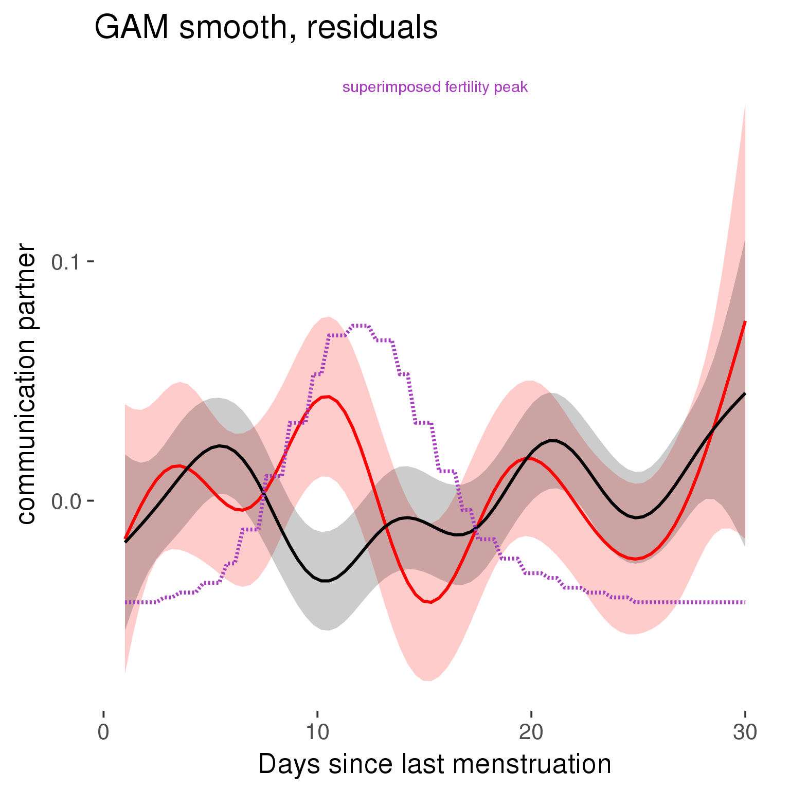
GAM smooth on raw data
As before, but without partialling anything out.
tryCatch({
trend_plot = ggplot(tmp,aes_string(x = "RCD", y = outcome, colour = "included")) +
stat_smooth(geom = 'smooth',size = 0.8, fill = "#9ECAE1", method = 'gam', formula = y ~ s(x))
}, error = function(e){cat_message(e, "danger")})
tryCatch({
trend_data = ggplot_build(trend_plot)$data[[1]]
}, error = function(e){cat_message(e, "danger")})
trend_data$RCD = round(trend_data$x)
trend_data = left_join(trend_data, tmp %>% select(real, RCD,fertile) %>% unique(), by = "RCD")
trend_data %>%
filter(real == TRUE) %>%
mutate(superimposed = ( ( (fertile - 0.01)/0.58) * (max(y)-min(y) ) ) + min(y) ) ->
trend_data
plot1b = ggplot(trend_data) +
geom_ribbon(aes(x = x, ymin = ymin, ymax = ymax, fill = factor(group)), alpha = 0.2) +
geom_line(aes(x = x, y = y, colour = factor(group)), size = 0.8, stat = "identity") +
scale_x_continuous(caption_x) +
geom_line(aes(x = x, y = superimposed), color = "#a83fbf", size = 1, linetype = 'dashed') +
annotate("text",x = mean(trend_data$x), y = max(trend_data$superimposed,na.rm=T) + 0.1, label = 'superimposed fertility peak', color = "#a83fbf") +
scale_y_continuous(outcome_label) +
ggtitle("GAM smooth, raw data") +
scale_color_manual("Contraception status",values = c("2"="black","1"= "red"), labels = c("2"="hormonally\ncontracepting","1"="cycling"), guide = F) +
scale_fill_manual("Contraception status",values = c("2"="black","1"= "red"), labels = c("2"="hormonally\ncontracepting","1"="cycling"), guide = F)
suppressWarnings(print(plot1b))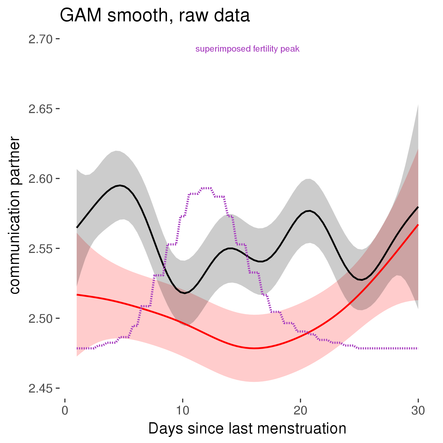
Means and standard errors over raw data
Nothing partialled out, just straight means with bootstrapped confidence intervals.
tryCatch({
trend_plot = ggplot(tmp,aes_string(x = "RCD", y = outcome, colour = "included")) +
geom_pointrange(size = 0.8, stat = 'summary', fun.data = "mean_cl_boot")
}, error = function(e){cat_message(e, "danger")})
tryCatch({
trend_data = ggplot_build(trend_plot)$data[[1]]
}, error = function(e){cat_message(e, "danger")})
trend_data$RCD = round(trend_data$x)
trend_data = left_join(trend_data, tmp %>% select(real, RCD,fertile) %>% unique(), by = "RCD")
trend_data %>%
filter(real == TRUE) %>%
mutate(superimposed = ( ( (fertile - 0.01)/0.58) * (max(y)-min(y) ) ) + min(y) ) ->
trend_data
plot3 = ggplot(trend_data) +
geom_pointrange(aes(x = x, y = y, ymin = ymin,ymax = ymax, colour = factor(group)), size = 0.8, stat = "identity", alpha = 0.6, position = position_dodge(width = .5)) +
scale_x_continuous("Days until next menstruation") +
geom_line(aes(x= x, y = superimposed), color = "#a83fbf", size = 1, linetype = 'dashed') +
annotate("text",x = mean(trend_data$x), y = max(trend_data$superimposed,na.rm=T) + 0.1, label = 'superimposed fertility peak', color = "#a83fbf") +
scale_y_continuous(outcome_label) +
ggtitle("Means with standard errors, raw data") +
scale_color_manual("Contraception status",values = c("2"="black","1"= "red"), labels = c("2"="hormonally\ncontracepting","1"="cycling"), guide = F) +
scale_fill_manual("Contraception status",values = c("2"="black","1"= "red"), labels = c("2"="hormonally\ncontracepting","1"="cycling"), guide = F)
suppressWarnings(print(plot3))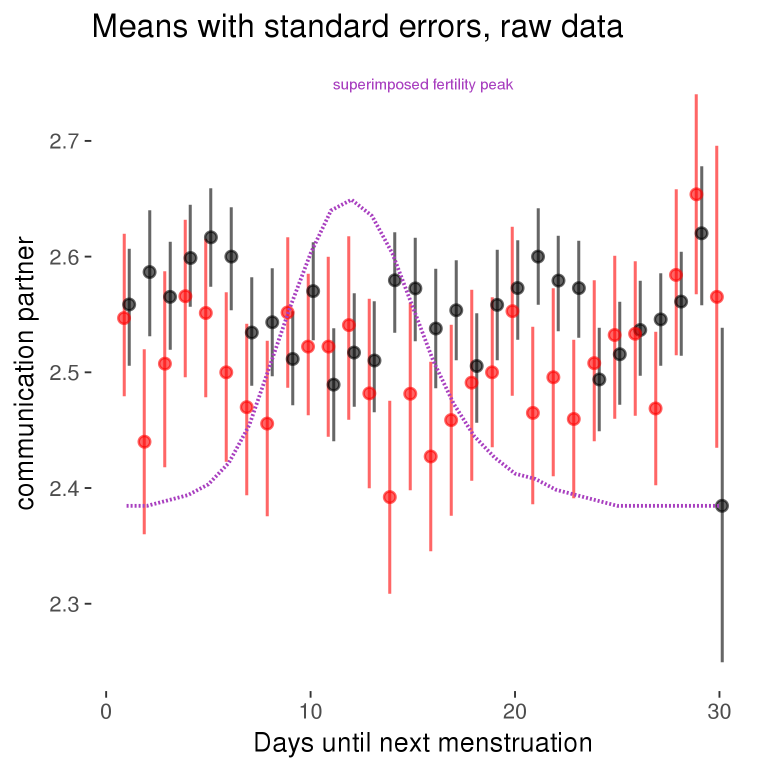
Robustness checks
M_r1: Random slopes for conception risk and menstruation
tryCatch({
# refit model with random effects for fertile and menstruation dummies
with_ind_diff = update(model, formula = . ~ . - (1| person) + (1 + fertile + menstruation | person))
# pull the random effects, format as tibble
rand = coef(with_ind_diff)$person %>%
tibble::rownames_to_column("person") %>%
mutate(person = as.numeric(person))
# pull the fixed effects
fixd = data.frame(fixef(with_ind_diff)) %>%
tibble::rownames_to_column("effect")
names(fixd) = c("effect", "pop_effect_size")
# pull apart the coefficients so that we can account for the fact that the random effect variation implicitly includes HC explaining the mean population-level effect of fertile/menstruation dummies among HC users
fixd = fixd %>%
separate(effect, c("included", "effect"), sep = ":", fill = "left") %>%
mutate(included = if_else(is.na(included), "cycling", str_replace(included, "included", "")))
fixd[2,c("included", "effect")] = c("horm_contra", "(Intercept)")
rand = rand %>%
# merge diary data on the random effects, so that we know who is a HC users and who isn't
inner_join(diary %>% select(person, included) %>% unique(), by = 'person') %>%
# gather into long format, to have the dataset by predictor
gather(effect, value, -person, -included) %>%
inner_join(fixd, by = c('effect', 'included')) %>%
# pull the fixed effects
mutate(
# only for those who are HC users, add the moderated population effect size for this effect (the random effects have the reference category mean)
value = if_else(included == "horm_contra", value + pop_effect_size, value),
effect = recode(effect, "includedhorm_contra" = "HC user",
"includedhorm_contra:fertile" = "HC user x fertile",
"includedhorm_contra:menstruationpre" = "HC user x premens.",
"includedhorm_contra:menstruationyes" = "HC user x mens.",
"menstruationyes" = "mens.",
"menstruationpre" = "premens.")) %>%
group_by(included, effect) %>%
# filter out predictors that aren't modelled as varying/random
filter(sd(value) > 0)
# plot dot plot of random effects
print(
ggplot(rand, aes(x = included, y = value, color = included, fill = included)) +
facet_wrap( ~ effect, scales = "free") +
# geom_violin(alpha = 0.4, size = 0) +
geom_dotplot(binaxis='y', dotsize = 0.1, method = "histodot") +
# geom_jitter(alpha = 0.05) +
coord_flip() +
geom_pointrange(stat = 'summary', fun.data = 'mean_sdl', color = 'darkred', size = 1.2) +
scale_color_manual("Contraception status", values = c("horm_contra"="black","cycling"= "red"), labels = c("horm_contra"="hormonally\ncontracepting","cycling"="cycling"), guide = F) +
scale_fill_manual("Contraception status", values = c("horm_contra"="black","cycling"= "red"), labels = c("horm_contra"="hormonally\ncontracepting","1"="cycling"), guide = F) +
ggtitle("M_r1: allowing participant-varying slopes", subtitle = "for the conception risk measure and the menstruation dummies") +
scale_x_discrete("Hormonal contraception", breaks = c("horm_contra", "cycling"), labels = c("yes", "no")) +
scale_y_continuous("Random effect size distribution"))
print_summary(with_ind_diff)
cat(pander(anova(model, with_ind_diff)))
}, error = function(e){
with_ind_diff = model
cat_message(e, "danger")
})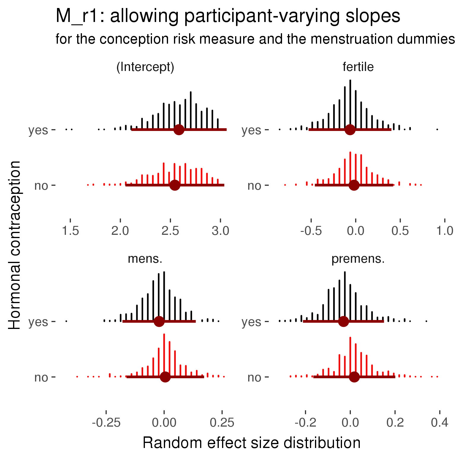
Linear mixed model fit by REML ['lmerMod']
Formula: communication_partner_1 ~ included + menstruation + fertile +
fertile_mean + (1 + fertile + menstruation | person) + included:menstruation + included:fertile
Data: diary
REML criterion at convergence: 40648
Scaled residuals:
Min 1Q Median 3Q Max
-3.723 -0.832 0.238 0.768 2.875
Random effects:
Groups Name Variance Std.Dev. Corr
person (Intercept) 0.0811 0.285
fertile 0.1734 0.416 -0.40
menstruationpre 0.0331 0.182 -0.38 0.48
menstruationyes 0.0274 0.165 -0.26 0.60 0.55
Residual 0.2402 0.490
Number of obs: 26704, groups: person, 1054
Fixed effects:
Estimate Std. Error t value
(Intercept) 2.54455 0.02662 95.6
includedhorm_contra 0.04081 0.02262 1.8
menstruationpre 0.01808 0.01824 1.0
menstruationyes 0.00497 0.01700 0.3
fertile -0.01883 0.03833 -0.5
fertile_mean -0.09586 0.12128 -0.8
includedhorm_contra:menstruationpre -0.04809 0.02342 -2.1
includedhorm_contra:menstruationyes -0.02632 0.02214 -1.2
includedhorm_contra:fertile -0.04424 0.04859 -0.9
Correlation of Fixed Effects:
(Intr) incld_ mnstrtnp mnstrtny fertil frtl_m inclddhrm_cntr:mnstrtnp
inclddhrm_c -0.495
menstrutnpr -0.303 0.359
menstrutnys -0.256 0.312 0.435
fertile -0.286 0.423 0.462 0.449
fertile_men -0.749 -0.030 -0.002 -0.012 -0.096
inclddhrm_cntr:mnstrtnp 0.246 -0.452 -0.779 -0.339 -0.358 -0.011
inclddhrm_cntr:mnstrtny 0.208 -0.386 -0.334 -0.767 -0.343 -0.005 0.424
inclddhrm_cntr:f 0.273 -0.537 -0.364 -0.353 -0.783 0.012 0.462
inclddhrm_cntr:mnstrtny
inclddhrm_c
menstrutnpr
menstrutnys
fertile
fertile_men
inclddhrm_cntr:mnstrtnp
inclddhrm_cntr:mnstrtny
inclddhrm_cntr:f 0.445
refitting model(s) with ML (instead of REML)
| Df | AIC | BIC | logLik | deviance | Chisq | Chi Df | Pr(>Chisq) | |
|---|---|---|---|---|---|---|---|---|
| object | 11 | 40814 | 40904 | -20396 | 40792 | NA | NA | NA |
| ..1 | 20 | 40635 | 40799 | -20298 | 40595 | 197.1 | 9 | 1.315e-37 |
robustness_check_ovu_shift(model, diary)M_e: Exclusion criteria
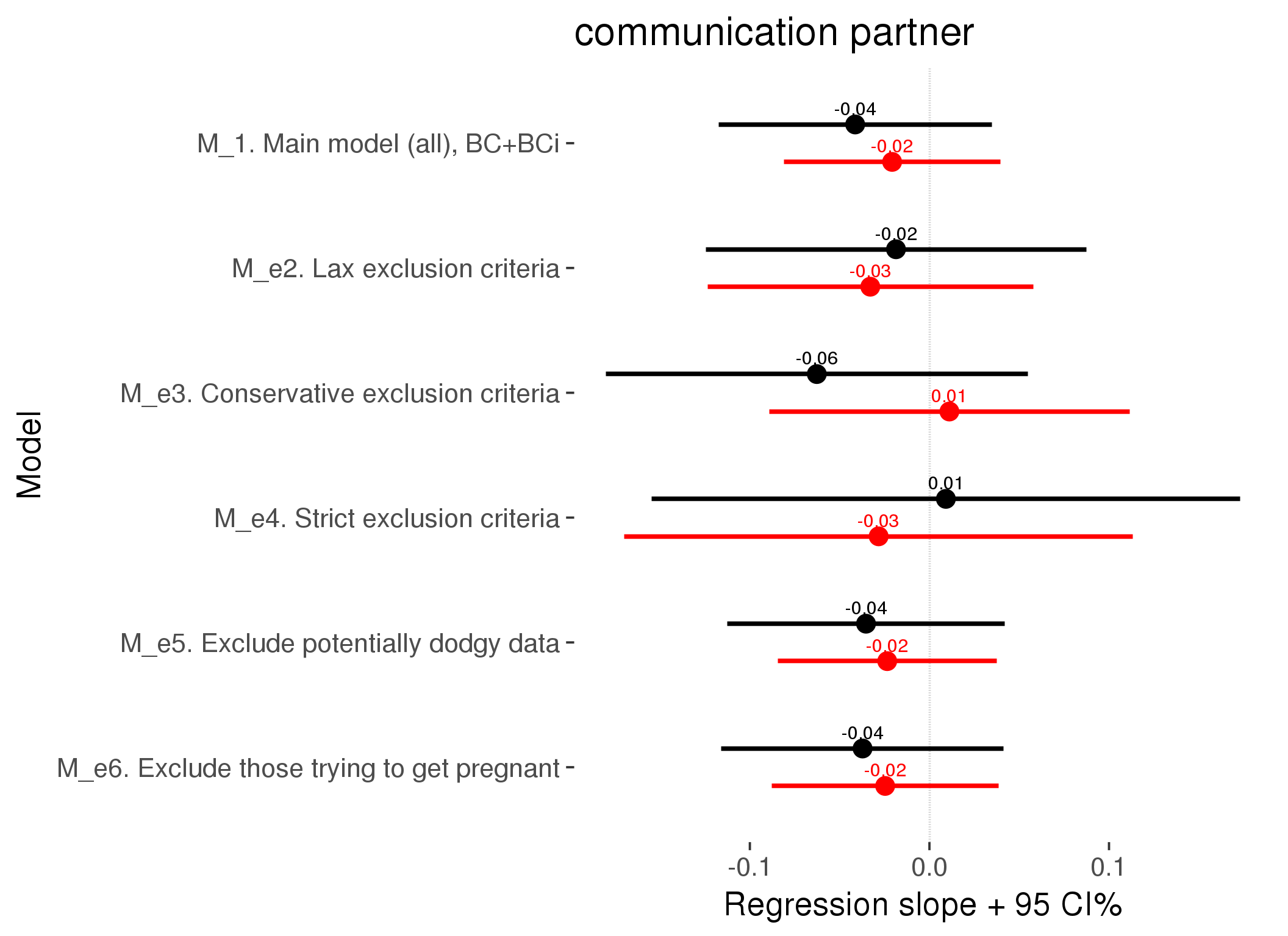
M_p: Predictors
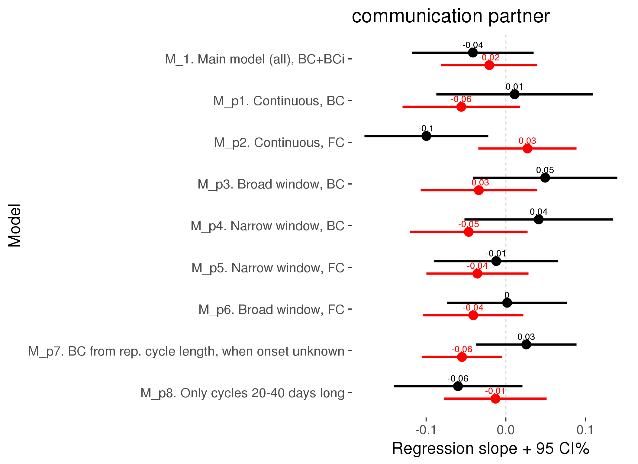
M_c: Covariates, controls, autocorrelation
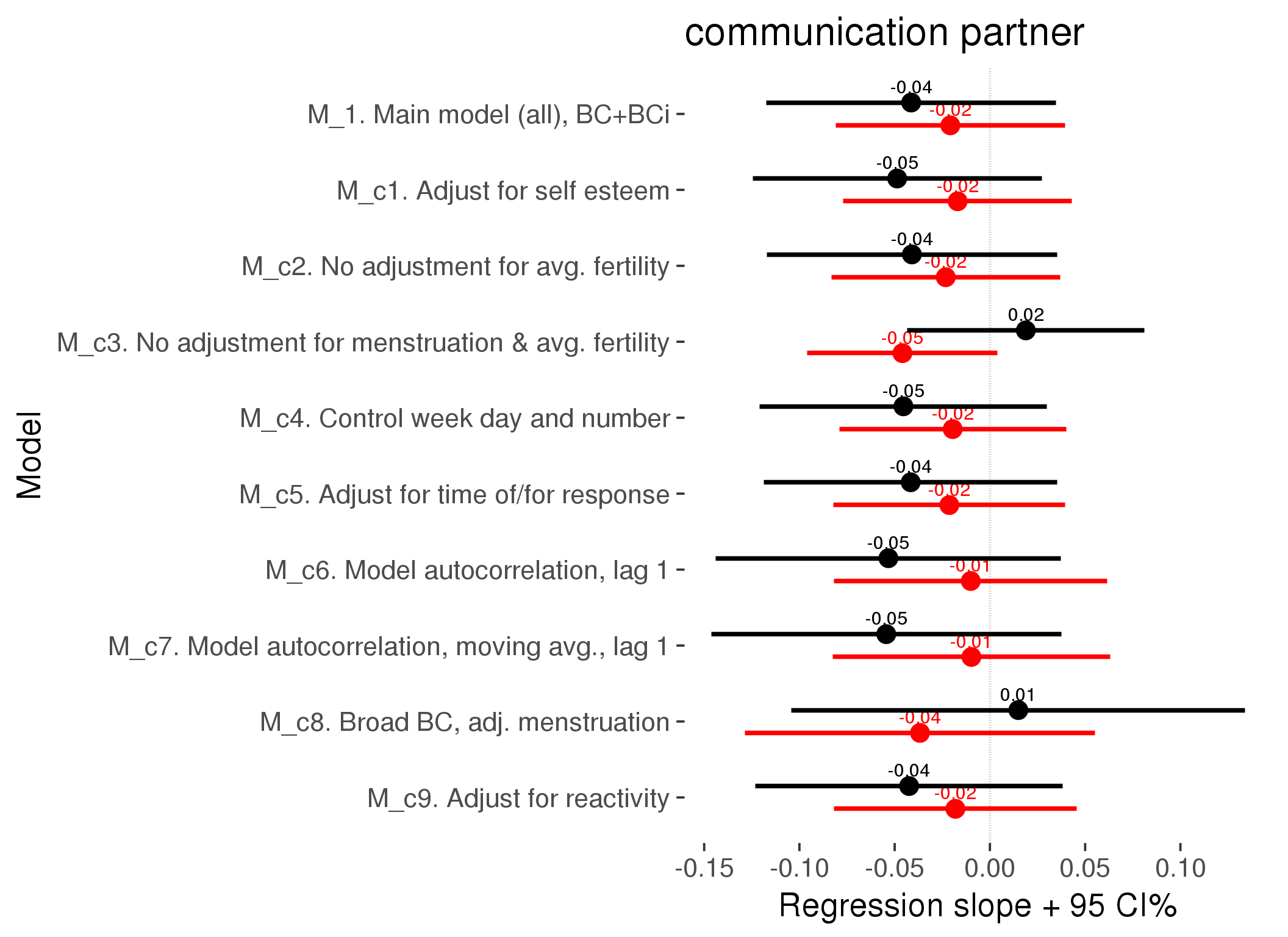
Linear mixed model fit by REML ['lmerMod']
REML criterion at convergence: 37241
Scaled residuals:
Min 1Q Median 3Q Max
-3.704 -0.842 0.252 0.785 2.821
Random effects:
Groups Name Variance Std.Dev.
person (Intercept) 0.06777 0.2603
Xr.2 s(days_filled_out):includedhorm_contra 0.00126 0.0355
Xr.1 s(days_filled_out):includedcycling 0.00445 0.0667
Xr.0 s(day_number):includedhorm_contra 0.00000 0.0000
Xr s(day_number):includedcycling 0.00000 0.0000
Residual 0.24829 0.4983
Number of obs: 24398, groups: person, 1054; Xr.2, 8; Xr.1, 8; Xr.0, 8; Xr, 8
Fixed effects:
Estimate Std. Error t value
X(Intercept) 2.54213 0.02618 97.1
Xincludedhorm_contra 0.03760 0.02175 1.7
Xmenstruationpre 0.02516 0.01582 1.6
Xmenstruationyes 0.00982 0.01516 0.6
Xfertile -0.01811 0.03256 -0.6
Xfertile_mean -0.12040 0.12037 -1.0
Xincludedhorm_contra:menstruationpre -0.05375 0.02028 -2.7
Xincludedhorm_contra:menstruationyes -0.02918 0.01984 -1.5
Xincludedhorm_contra:fertile -0.04241 0.04114 -1.0
Xs(day_number):includedcyclingFx1 0.02132 0.02457 0.9
Xs(day_number):includedhorm_contraFx1 0.07788 0.02100 3.7
Xs(days_filled_out):includedcyclingFx1 -0.00272 0.03362 -0.1
Xs(days_filled_out):includedhorm_contraFx1 -0.09892 0.02485 -4.0
Family: gaussian
Link function: identity
Formula:
communication_partner_1 ~ included + menstruation + fertile +
fertile_mean + s(day_number, by = included) + s(days_filled_out,
by = included) + included:menstruation + included:fertile
Parametric coefficients:
Estimate Std. Error t value Pr(>|t|)
(Intercept) 2.54213 0.02618 97.10 <2e-16 ***
includedhorm_contra 0.03760 0.02175 1.73 0.084 .
menstruationpre 0.02516 0.01582 1.59 0.112
menstruationyes 0.00982 0.01516 0.65 0.517
fertile -0.01811 0.03256 -0.56 0.578
fertile_mean -0.12040 0.12037 -1.00 0.317
includedhorm_contra:menstruationpre -0.05375 0.02028 -2.65 0.008 **
includedhorm_contra:menstruationyes -0.02918 0.01984 -1.47 0.141
includedhorm_contra:fertile -0.04241 0.04114 -1.03 0.303
---
Signif. codes: 0 '***' 0.001 '**' 0.01 '*' 0.05 '.' 0.1 ' ' 1
Approximate significance of smooth terms:
edf Ref.df F p-value
s(day_number):includedcycling 1.00 1.00 0.75 0.38548
s(day_number):includedhorm_contra 1.00 1.00 13.75 0.00021 ***
s(days_filled_out):includedcycling 2.69 2.69 1.88 0.08881 .
s(days_filled_out):includedhorm_contra 2.20 2.20 10.67 0.000015 ***
---
Signif. codes: 0 '***' 0.001 '**' 0.01 '*' 0.05 '.' 0.1 ' ' 1
R-sq.(adj) = 0.00133
lmer.REML = 37241 Scale est. = 0.24829 n = 24398
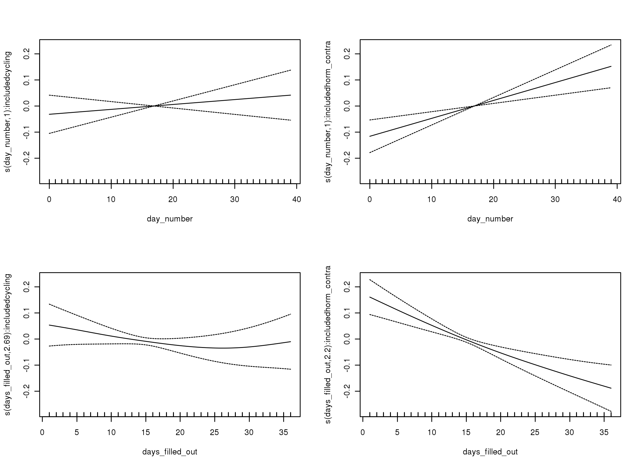
Linear mixed-effects model fit by REML
Data: diary
AIC BIC logLik
39515 39614 -19746
Random effects:
Formula: ~1 | person
(Intercept) Residual
StdDev: 0.2464 0.5058
Correlation Structure: ARMA(1,0)
Formula: ~day_number | person
Parameter estimate(s):
Phi1
0.2624
Fixed effects: communication_partner_1 ~ included * (menstruation + fertile) + fertile_mean
Value Std.Error DF t-value p-value
(Intercept) 2.5469 0.02639 25644 96.51 0.0000
includedhorm_contra 0.0411 0.02190 1051 1.88 0.0607
menstruationpre 0.0155 0.01736 25644 0.89 0.3718
menstruationyes 0.0052 0.01619 25644 0.32 0.7487
fertile -0.0101 0.03660 25644 -0.27 0.7834
fertile_mean -0.0940 0.12238 1051 -0.77 0.4426
includedhorm_contra:menstruationpre -0.0490 0.02229 25644 -2.20 0.0279
includedhorm_contra:menstruationyes -0.0193 0.02112 25644 -0.91 0.3609
includedhorm_contra:fertile -0.0533 0.04620 25644 -1.15 0.2488
Correlation:
(Intr) incld_ mnstrtnp mnstrtny fertil frtl_m inclddhrm_cntr:mnstrtnp
includedhorm_contra -0.482
menstruationpre -0.258 0.316
menstruationyes -0.249 0.304 0.397
fertile -0.244 0.394 0.432 0.363
fertile_mean -0.761 -0.032 -0.005 -0.004 -0.105
includedhorm_contra:menstruationpre 0.210 -0.394 -0.779 -0.309 -0.335 -0.008
includedhorm_contra:menstruationyes 0.198 -0.371 -0.304 -0.766 -0.277 -0.007 0.382
includedhorm_contra:fertile 0.246 -0.499 -0.342 -0.287 -0.785 0.015 0.432
inclddhrm_cntr:mnstrtny
includedhorm_contra
menstruationpre
menstruationyes
fertile
fertile_mean
includedhorm_contra:menstruationpre
includedhorm_contra:menstruationyes
includedhorm_contra:fertile 0.357
Standardized Within-Group Residuals:
Min Q1 Med Q3 Max
-3.6667 -0.8653 0.2896 0.7830 2.7738
Number of Observations: 26704
Number of Groups: 1054
Linear mixed-effects model fit by REML
Data: diary
AIC BIC logLik
39499 39605 -19736
Random effects:
Formula: ~1 | person
(Intercept) Residual
StdDev: 0.2449 0.5064
Correlation Structure: ARMA(1,1)
Formula: ~day_number | person
Parameter estimate(s):
Phi1 Theta1
0.3697 -0.1149
Fixed effects: communication_partner_1 ~ included * (menstruation + fertile) + fertile_mean
Value Std.Error DF t-value p-value
(Intercept) 2.5468 0.02645 25644 96.28 0.0000
includedhorm_contra 0.0412 0.02197 1051 1.88 0.0610
menstruationpre 0.0150 0.01749 25644 0.86 0.3905
menstruationyes 0.0046 0.01633 25644 0.28 0.7792
fertile -0.0097 0.03713 25644 -0.26 0.7936
fertile_mean -0.0933 0.12270 1051 -0.76 0.4473
includedhorm_contra:menstruationpre -0.0487 0.02247 25644 -2.17 0.0303
includedhorm_contra:menstruationyes -0.0188 0.02129 25644 -0.88 0.3782
includedhorm_contra:fertile -0.0544 0.04686 25644 -1.16 0.2455
Correlation:
(Intr) incld_ mnstrtnp mnstrtny fertil frtl_m inclddhrm_cntr:mnstrtnp
includedhorm_contra -0.482
menstruationpre -0.259 0.316
menstruationyes -0.251 0.305 0.400
fertile -0.245 0.397 0.425 0.360
fertile_mean -0.761 -0.033 -0.005 -0.004 -0.107
includedhorm_contra:menstruationpre 0.210 -0.394 -0.778 -0.311 -0.330 -0.008
includedhorm_contra:menstruationyes 0.200 -0.373 -0.307 -0.767 -0.275 -0.007 0.385
includedhorm_contra:fertile 0.247 -0.502 -0.336 -0.285 -0.785 0.015 0.424
inclddhrm_cntr:mnstrtny
includedhorm_contra
menstruationpre
menstruationyes
fertile
fertile_mean
includedhorm_contra:menstruationpre
includedhorm_contra:menstruationyes
includedhorm_contra:fertile 0.354
Standardized Within-Group Residuals:
Min Q1 Med Q3 Max
-3.6564 -0.8666 0.2971 0.7836 2.7491
Number of Observations: 26704
Number of Groups: 1054
M_d: Other designs
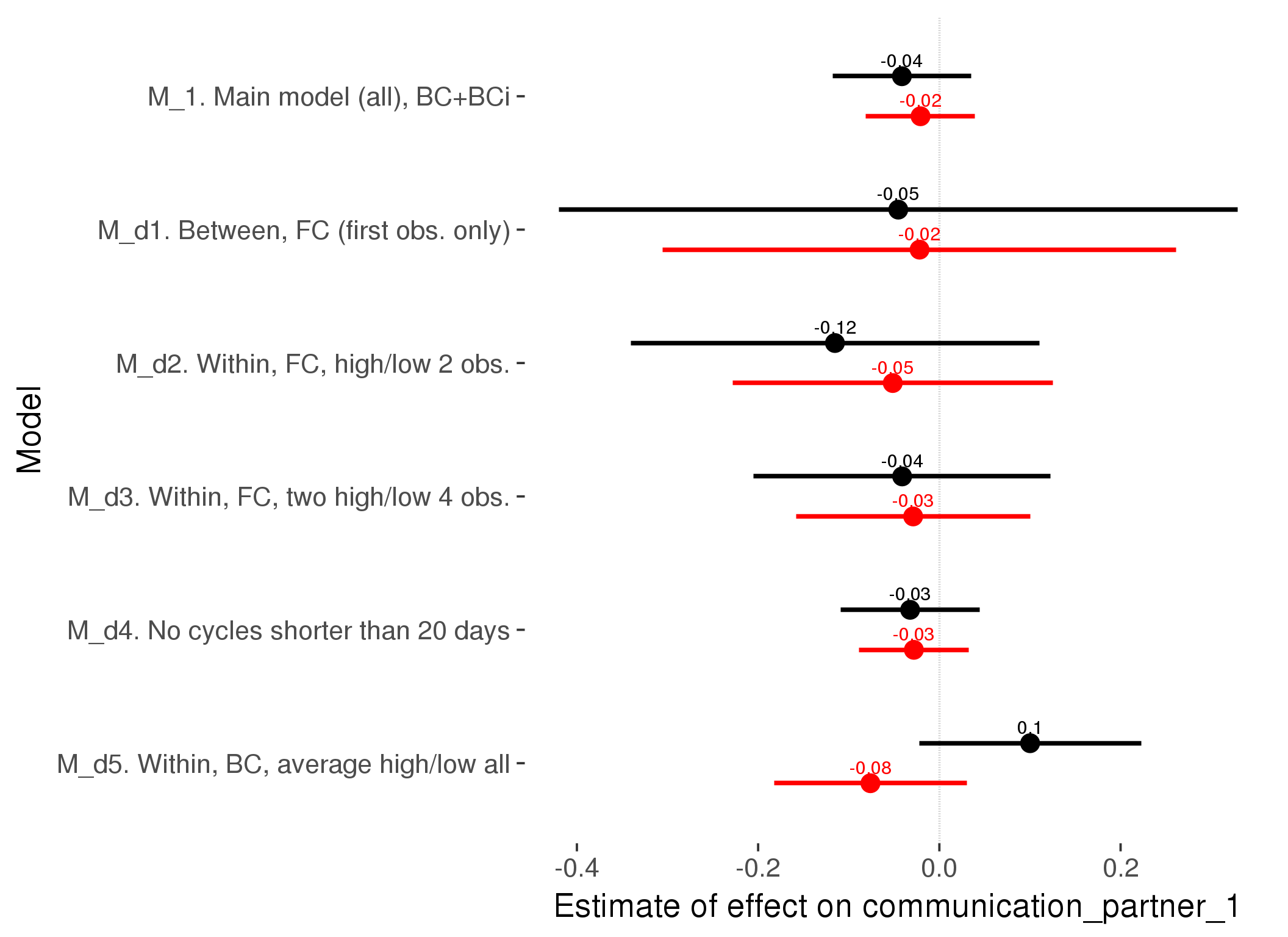
M_m1: Moderation by contraceptive method
Based on the sample with lax exclusion criteria. Users who used any hormonal contraception are classified as hormonal, users who use any awareness-based methods (counting, temperature-based) are classified as ‘fertility-awareness’, women who don’t fall into the before groups and use condoms, pessars, coitus interruptus etc. are classified as ‘barrie or abstinence’. Women who don’t use contraception or use other methods such as sterilisation are excluded from this analysis.
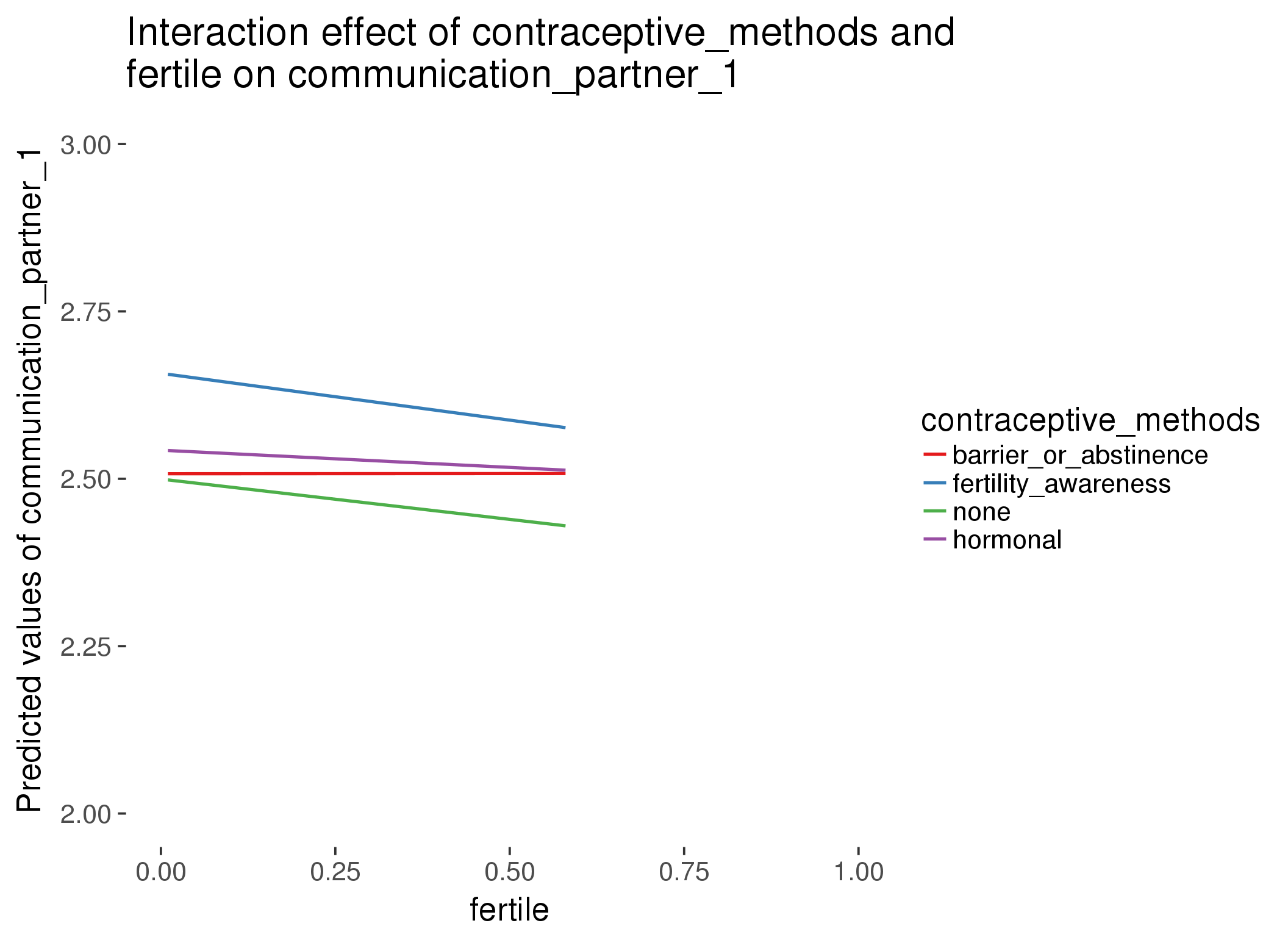
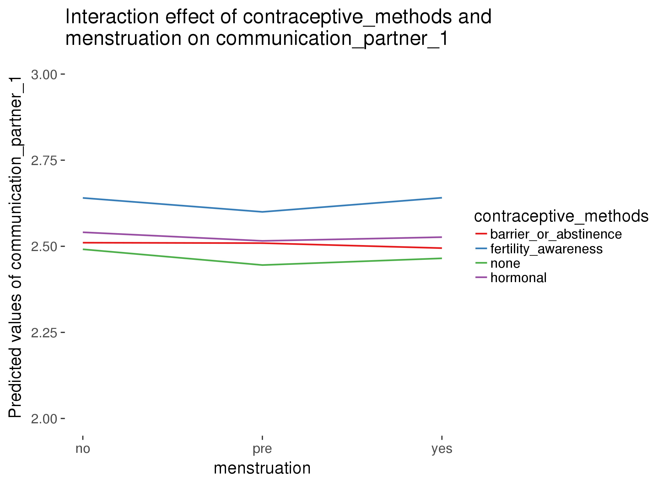
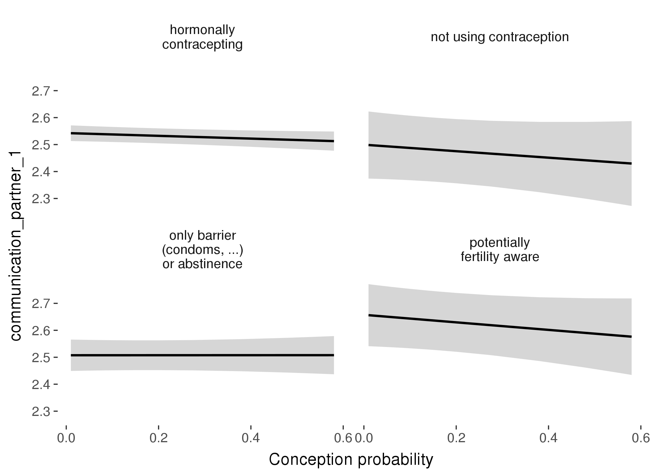
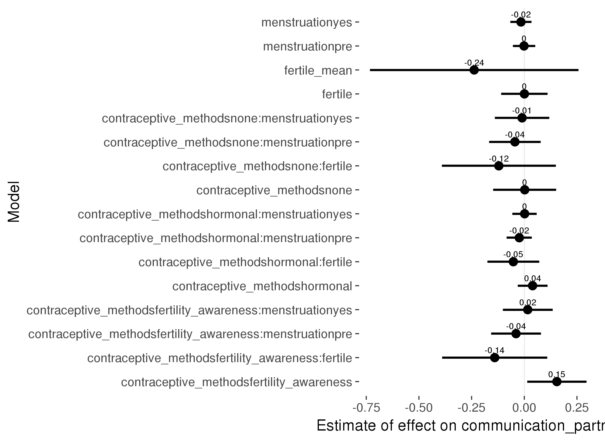
Linear mixed model fit by REML ['lmerMod']
Formula: communication_partner_1 ~ fertile_mean + (1 | person) + contraceptive_methods +
fertile + menstruation + fertile:contraceptive_methods + menstruation:contraceptive_methods
Data: diary
Subset: !is.na(included_lax) & contraceptive_method != "other"
REML criterion at convergence: 26215
Scaled residuals:
Min 1Q Median 3Q Max
-3.701 -0.843 0.243 0.783 2.886
Random effects:
Groups Name Variance Std.Dev.
person (Intercept) 0.0663 0.257
Residual 0.2538 0.504
Number of obs: 17044, groups: person, 513
Fixed effects:
Estimate Std. Error t value
(Intercept) 2.552029 0.052748 48.4
fertile_mean -0.237851 0.252436 -0.9
contraceptive_methodsfertility_awareness 0.154581 0.071903 2.1
contraceptive_methodsnone 0.002050 0.076230 0.0
contraceptive_methodshormonal 0.039372 0.036111 1.1
fertile 0.000541 0.056093 0.0
menstruationpre -0.001261 0.027092 0.0
menstruationyes -0.015761 0.025855 -0.6
contraceptive_methodsfertility_awareness:fertile -0.140399 0.127420 -1.1
contraceptive_methodsnone:fertile -0.120908 0.138004 -0.9
contraceptive_methodshormonal:fertile -0.052020 0.062634 -0.8
contraceptive_methodsfertility_awareness:menstruationpre -0.039217 0.060068 -0.7
contraceptive_methodsnone:menstruationpre -0.044501 0.062747 -0.7
contraceptive_methodshormonal:menstruationpre -0.023694 0.030515 -0.8
contraceptive_methodsfertility_awareness:menstruationyes 0.016308 0.060343 0.3
contraceptive_methodsnone:menstruationyes -0.010447 0.065642 -0.2
contraceptive_methodshormonal:menstruationyes 0.001625 0.029482 0.1
refitting model(s) with ML (instead of REML)
| Df | AIC | BIC | logLik | deviance | Chisq | Chi Df | Pr(>Chisq) | |
|---|---|---|---|---|---|---|---|---|
| add_main | 13 | 26167 | 26268 | -13071 | 26141 | NA | NA | NA |
| by_method | 19 | 26177 | 26324 | -13069 | 26139 | 2.618 | 6 | 0.8551 |
M_m2: Moderation by participant age
model %>%
test_moderator("age_group", diary, xlevels = 5)refitting model(s) with ML (instead of REML)
| Df | AIC | BIC | logLik | deviance | Chisq | Chi Df | Pr(>Chisq) | |
|---|---|---|---|---|---|---|---|---|
| with_main | 19 | 40825 | 40981 | -20393 | 40787 | NA | NA | NA |
| with_mod | 27 | 40832 | 41053 | -20389 | 40778 | 9.377 | 8 | 0.3115 |
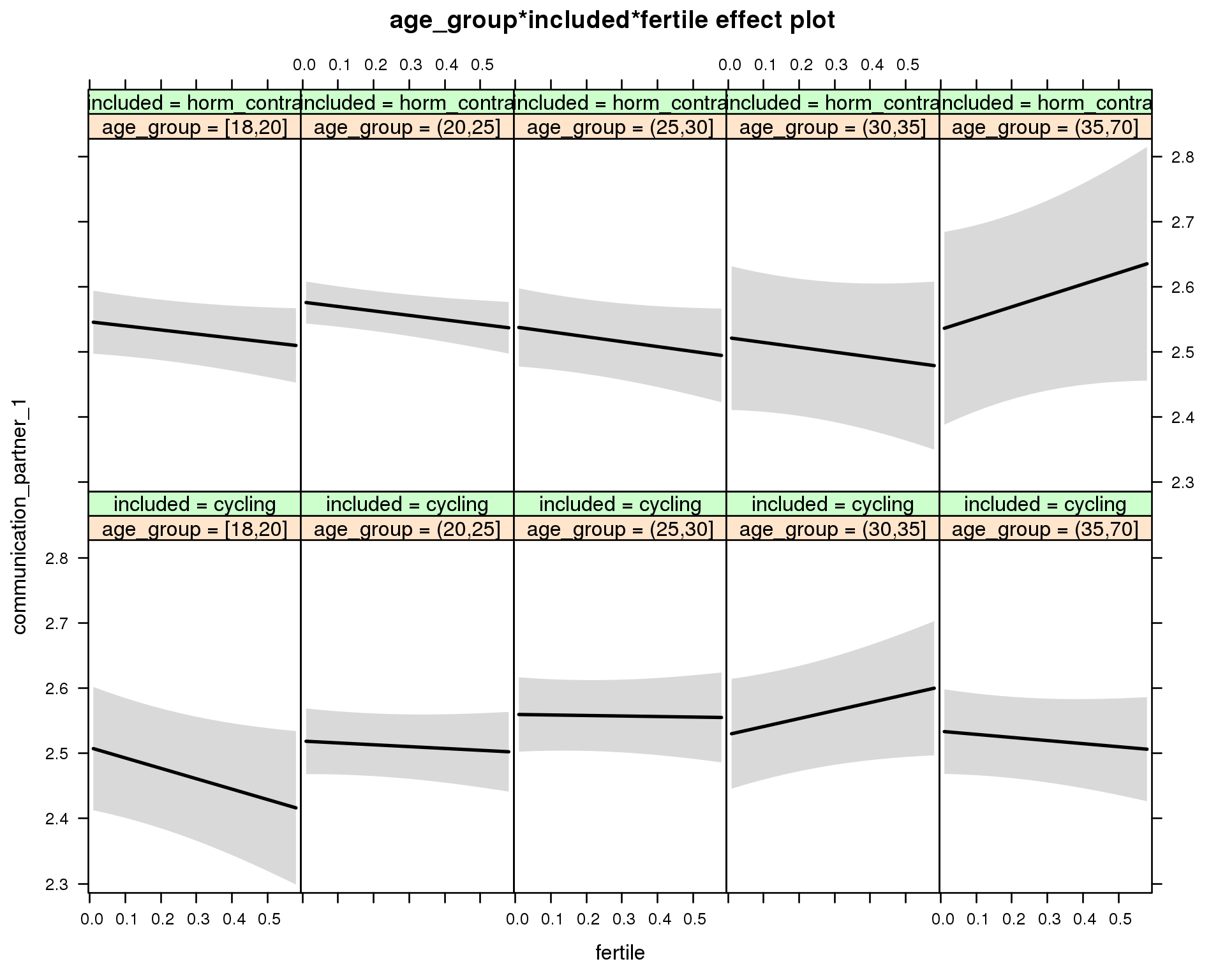
Linear mixed model fit by REML ['lmerMod']
Formula: communication_partner_1 ~ menstruation + fertile_mean + (1 |
person) + age_group + included + fertile + menstruation:included +
age_group:included + age_group:fertile + included:fertile + age_group:included:fertile
Data: diary
REML criterion at convergence: 40894
Scaled residuals:
Min 1Q Median 3Q Max
-3.741 -0.848 0.246 0.785 2.921
Random effects:
Groups Name Variance Std.Dev.
person (Intercept) 0.0669 0.259
Residual 0.2505 0.501
Number of obs: 26704, groups: person, 1054
Fixed effects:
Estimate Std. Error t value
(Intercept) 2.52337 0.05195 48.6
menstruationpre 0.01776 0.01522 1.2
menstruationyes 0.00628 0.01432 0.4
fertile_mean -0.10702 0.11979 -0.9
age_group(20,25] 0.00996 0.05485 0.2
age_group(25,30] 0.05088 0.05651 0.9
age_group(30,35] 0.02005 0.06484 0.3
age_group(35,70] 0.02501 0.05867 0.4
includedhorm_contra 0.05062 0.05523 0.9
fertile -0.15964 0.08789 -1.8
menstruationpre:includedhorm_contra -0.04985 0.01954 -2.6
menstruationyes:includedhorm_contra -0.02778 0.01878 -1.5
age_group(20,25]:includedhorm_contra 0.02032 0.06240 0.3
age_group(25,30]:includedhorm_contra -0.05876 0.06892 -0.9
age_group(30,35]:includedhorm_contra -0.04439 0.08949 -0.5
age_group(35,70]:includedhorm_contra -0.03668 0.09914 -0.4
age_group(20,25]:fertile 0.13137 0.09729 1.4
age_group(25,30]:fertile 0.15168 0.10030 1.5
age_group(30,35]:fertile 0.28232 0.11611 2.4
age_group(35,70]:fertile 0.11220 0.10483 1.1
includedhorm_contra:fertile 0.09706 0.09746 1.0
age_group(20,25]:includedhorm_contra:fertile -0.13674 0.10898 -1.3
age_group(25,30]:includedhorm_contra:fertile -0.16448 0.12074 -1.4
age_group(30,35]:includedhorm_contra:fertile -0.29372 0.15574 -1.9
age_group(35,70]:includedhorm_contra:fertile 0.12415 0.17715 0.7
M_m3: Moderation by weekend
model %>%
test_moderator("weekend", diary, xlevels = 2) refitting model(s) with ML (instead of REML)
| Df | AIC | BIC | logLik | deviance | Chisq | Chi Df | Pr(>Chisq) | |
|---|---|---|---|---|---|---|---|---|
| with_main | 13 | 40457 | 40564 | -20216 | 40431 | NA | NA | NA |
| with_mod | 15 | 40459 | 40582 | -20215 | 40429 | 1.542 | 2 | 0.4626 |
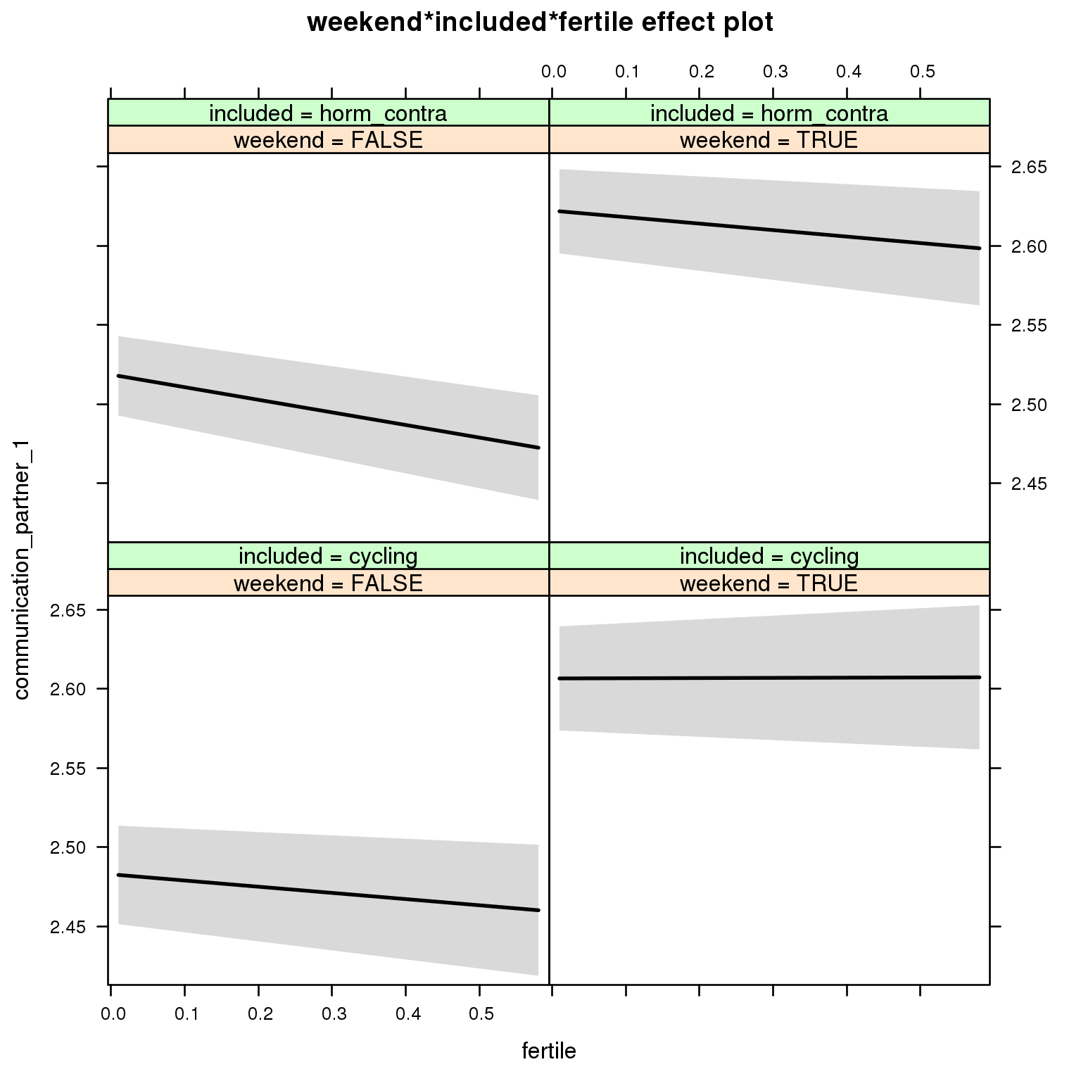
Linear mixed model fit by REML ['lmerMod']
Formula: communication_partner_1 ~ menstruation + fertile_mean + (1 |
person) + weekend + included + fertile + menstruation:included +
weekend:included + weekend:fertile + included:fertile + weekend:included:fertile
Data: diary
REML criterion at convergence: 40508
Scaled residuals:
Min 1Q Median 3Q Max
-3.903 -0.827 0.248 0.781 3.031
Random effects:
Groups Name Variance Std.Dev.
person (Intercept) 0.0668 0.258
Residual 0.2471 0.497
Number of obs: 26704, groups: person, 1054
Fixed effects:
Estimate Std. Error t value
(Intercept) 2.49630 0.02622 95.2
menstruationpre 0.01828 0.01511 1.2
menstruationyes 0.00585 0.01422 0.4
fertile_mean -0.10173 0.11901 -0.9
weekendTRUE 0.12373 0.01320 9.4
includedhorm_contra 0.04920 0.02215 2.2
fertile -0.03911 0.03714 -1.1
menstruationpre:includedhorm_contra -0.05074 0.01939 -2.6
menstruationyes:includedhorm_contra -0.02543 0.01863 -1.4
weekendTRUE:includedhorm_contra -0.02017 0.01699 -1.2
weekendTRUE:fertile 0.04033 0.05121 0.8
includedhorm_contra:fertile -0.04048 0.04713 -0.9
weekendTRUE:includedhorm_contra:fertile -0.00172 0.06513 0.0
M_m4: Moderation by weekday
model %>%
test_moderator("weekday", diary, xlevels = 7)refitting model(s) with ML (instead of REML)
| Df | AIC | BIC | logLik | deviance | Chisq | Chi Df | Pr(>Chisq) | |
|---|---|---|---|---|---|---|---|---|
| with_main | 23 | 40255 | 40443 | -20104 | 40209 | NA | NA | NA |
| with_mod | 35 | 40269 | 40556 | -20099 | 40199 | 9.569 | 12 | 0.6537 |
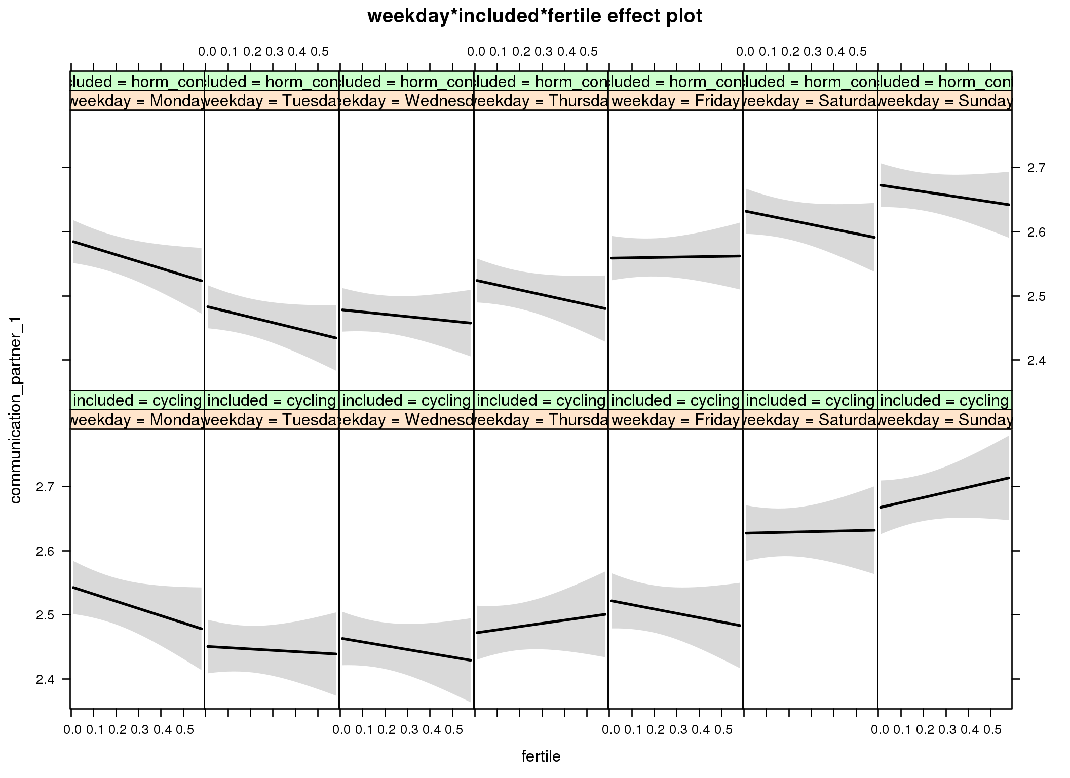
Linear mixed model fit by REML ['lmerMod']
Formula: communication_partner_1 ~ menstruation + fertile_mean + (1 |
person) + weekday + included + fertile + menstruation:included +
weekday:included + weekday:fertile + included:fertile + weekday:included:fertile
Data: diary
REML criterion at convergence: 40377
Scaled residuals:
Min 1Q Median 3Q Max
-3.903 -0.819 0.244 0.777 3.116
Random effects:
Groups Name Variance Std.Dev.
person (Intercept) 0.0671 0.259
Residual 0.2450 0.495
Number of obs: 26704, groups: person, 1054
Fixed effects:
Estimate Std. Error t value
(Intercept) 2.55921 0.02988 85.7
menstruationpre 0.01853 0.01505 1.2
menstruationyes 0.00579 0.01416 0.4
fertile_mean -0.11362 0.11898 -1.0
weekdayTuesday -0.09293 0.02353 -3.9
weekdayWednesday -0.08006 0.02350 -3.4
weekdayThursday -0.07204 0.02377 -3.0
weekdayFriday -0.02123 0.02417 -0.9
weekdaySaturday 0.08350 0.02441 3.4
weekdaySunday 0.12306 0.02360 5.2
includedhorm_contra 0.05508 0.02874 1.9
fertile -0.11282 0.06628 -1.7
menstruationpre:includedhorm_contra -0.05005 0.01932 -2.6
menstruationyes:includedhorm_contra -0.02431 0.01856 -1.3
weekdayTuesday:includedhorm_contra -0.00883 0.03023 -0.3
weekdayWednesday:includedhorm_contra -0.02700 0.03034 -0.9
weekdayThursday:includedhorm_contra 0.01115 0.03063 0.4
weekdayFriday:includedhorm_contra -0.00557 0.03105 -0.2
weekdaySaturday:includedhorm_contra -0.03658 0.03140 -1.2
weekdaySunday:includedhorm_contra -0.03556 0.03045 -1.2
weekdayTuesday:fertile 0.09236 0.09124 1.0
weekdayWednesday:fertile 0.05339 0.09169 0.6
weekdayThursday:fertile 0.16295 0.09300 1.8
weekdayFriday:fertile 0.04549 0.09316 0.5
weekdaySaturday:fertile 0.12088 0.09442 1.3
weekdaySunday:fertile 0.19338 0.09175 2.1
includedhorm_contra:fertile 0.00581 0.08474 0.1
weekdayTuesday:includedhorm_contra:fertile -0.07075 0.11647 -0.6
weekdayWednesday:includedhorm_contra:fertile 0.01748 0.11740 0.1
weekdayThursday:includedhorm_contra:fertile -0.13270 0.11834 -1.1
weekdayFriday:includedhorm_contra:fertile 0.06723 0.11869 0.6
weekdaySaturday:includedhorm_contra:fertile -0.08509 0.12043 -0.7
weekdaySunday:includedhorm_contra:fertile -0.13981 0.11721 -1.2
M_m5: Moderation by exclusion threshold
model %>%
test_moderator("included_levels", diary, xlevels = 4)refitting model(s) with ML (instead of REML)
| Df | AIC | BIC | logLik | deviance | Chisq | Chi Df | Pr(>Chisq) | |
|---|---|---|---|---|---|---|---|---|
| with_main | 17 | 40809 | 40948 | -20387 | 40775 | NA | NA | NA |
| with_mod | 23 | 40815 | 41004 | -20385 | 40769 | 5.518 | 6 | 0.4793 |
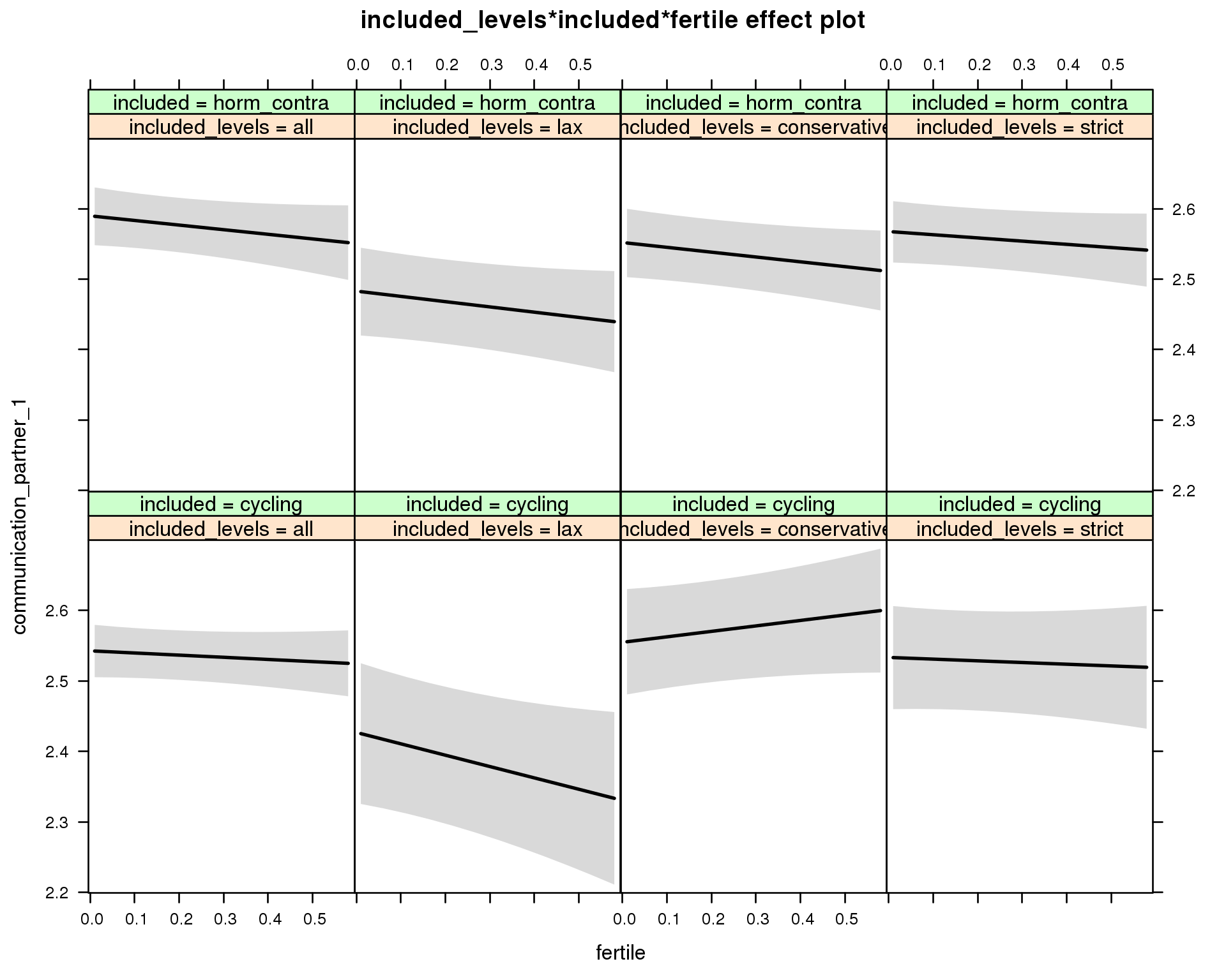
Linear mixed model fit by REML ['lmerMod']
Formula: communication_partner_1 ~ menstruation + fertile_mean + (1 |
person) + included_levels + included + fertile + menstruation:included +
included_levels:included + included_levels:fertile + included:fertile +
included_levels:included:fertile
Data: diary
REML criterion at convergence: 40875
Scaled residuals:
Min 1Q Median 3Q Max
-3.737 -0.847 0.247 0.786 2.934
Random effects:
Groups Name Variance Std.Dev.
person (Intercept) 0.066 0.257
Residual 0.251 0.501
Number of obs: 26704, groups: person, 1054
Fixed effects:
Estimate Std. Error t value
(Intercept) 2.55438 0.02841 89.9
menstruationpre 0.01860 0.01523 1.2
menstruationyes 0.00748 0.01432 0.5
fertile_mean -0.09445 0.12045 -0.8
included_levelslax -0.11586 0.05442 -2.1
included_levelsconservative 0.01213 0.04259 0.3
included_levelsstrict -0.00936 0.04184 -0.2
includedhorm_contra 0.06095 0.02943 2.1
fertile -0.03058 0.03876 -0.8
menstruationpre:includedhorm_contra -0.04981 0.01955 -2.5
menstruationyes:includedhorm_contra -0.02824 0.01878 -1.5
included_levelslax:includedhorm_contra 0.00908 0.06663 0.1
included_levelsconservative:includedhorm_contra -0.04995 0.05359 -0.9
included_levelsstrict:includedhorm_contra -0.01286 0.05183 -0.2
included_levelslax:fertile -0.13051 0.09495 -1.4
included_levelsconservative:fertile 0.10808 0.07083 1.5
included_levelsstrict:fertile 0.00651 0.07087 0.1
includedhorm_contra:fertile -0.03488 0.05889 -0.6
included_levelslax:includedhorm_contra:fertile 0.12129 0.11565 1.0
included_levelsconservative:includedhorm_contra:fertile -0.11110 0.09192 -1.2
included_levelsstrict:includedhorm_contra:fertile 0.01347 0.09049 0.1
M_m6: Moderation by cycle length
model %>%
test_moderator("cycle_length_groups", diary, xlevels = 4)refitting model(s) with ML (instead of REML)
| Df | AIC | BIC | logLik | deviance | Chisq | Chi Df | Pr(>Chisq) | |
|---|---|---|---|---|---|---|---|---|
| with_main | 17 | 40819 | 40958 | -20392 | 40785 | NA | NA | NA |
| with_mod | 23 | 40826 | 41014 | -20390 | 40780 | 4.732 | 6 | 0.5786 |
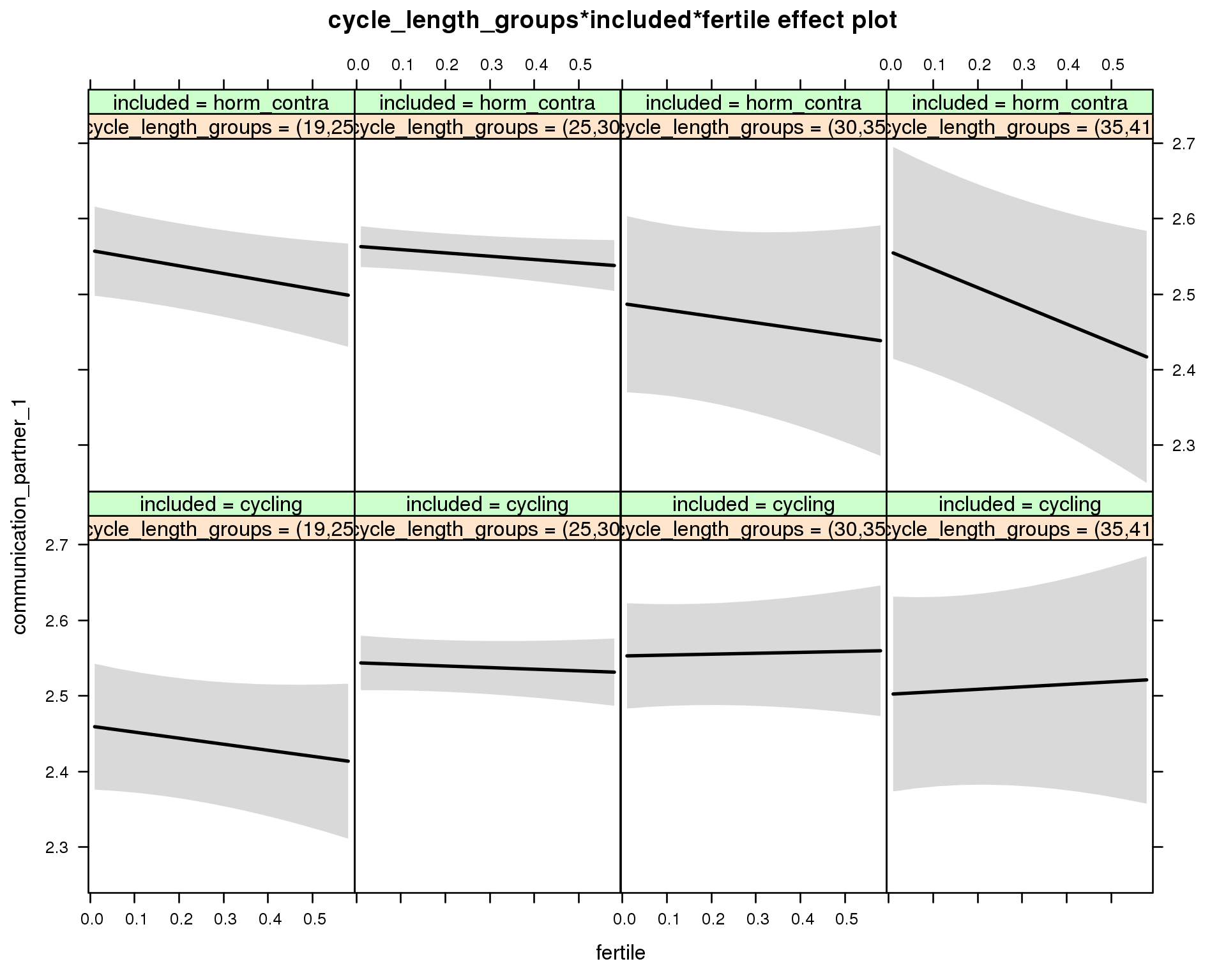
Linear mixed model fit by REML ['lmerMod']
Formula: communication_partner_1 ~ menstruation + fertile_mean + (1 |
person) + cycle_length_groups + included + fertile + menstruation:included +
cycle_length_groups:included + cycle_length_groups:fertile +
included:fertile + cycle_length_groups:included:fertile
Data: diary
REML criterion at convergence: 40878
Scaled residuals:
Min 1Q Median 3Q Max
-3.742 -0.848 0.247 0.784 2.936
Random effects:
Groups Name Variance Std.Dev.
person (Intercept) 0.0667 0.258
Residual 0.2505 0.501
Number of obs: 26704, groups: person, 1054
Fixed effects:
Estimate Std. Error t value
(Intercept) 2.475794 0.047749 51.9
menstruationpre 0.018490 0.015234 1.2
menstruationyes 0.008381 0.014422 0.6
fertile_mean -0.118326 0.120627 -1.0
cycle_length_groups(25,30] 0.083803 0.046460 1.8
cycle_length_groups(30,35] 0.092805 0.055581 1.7
cycle_length_groups(35,41] 0.042118 0.078603 0.5
includedhorm_contra 0.111578 0.052963 2.1
fertile -0.079923 0.080947 -1.0
menstruationpre:includedhorm_contra -0.049674 0.019550 -2.5
menstruationyes:includedhorm_contra -0.027966 0.018878 -1.5
cycle_length_groups(25,30]:includedhorm_contra -0.078366 0.057093 -1.4
cycle_length_groups(30,35]:includedhorm_contra -0.163154 0.086903 -1.9
cycle_length_groups(35,41]:includedhorm_contra -0.043052 0.110531 -0.4
cycle_length_groups(25,30]:fertile 0.058584 0.086830 0.7
cycle_length_groups(30,35]:fertile 0.091799 0.102865 0.9
cycle_length_groups(35,41]:fertile 0.112744 0.145291 0.8
includedhorm_contra:fertile -0.022163 0.095586 -0.2
cycle_length_groups(25,30]:includedhorm_contra:fertile -0.000271 0.102925 0.0
cycle_length_groups(30,35]:includedhorm_contra:fertile -0.074249 0.162082 -0.5
cycle_length_groups(35,41]:includedhorm_contra:fertile -0.251876 0.191399 -1.3
M_m7: Moderation by certainty about menstruation parameters
model %>%
test_moderator("certainty_menstruation", diary)refitting model(s) with ML (instead of REML)
| Df | AIC | BIC | logLik | deviance | Chisq | Chi Df | Pr(>Chisq) | |
|---|---|---|---|---|---|---|---|---|
| with_main | 13 | 40800 | 40906 | -20387 | 40774 | NA | NA | NA |
| with_mod | 15 | 40802 | 40925 | -20386 | 40772 | 1.381 | 2 | 0.5014 |
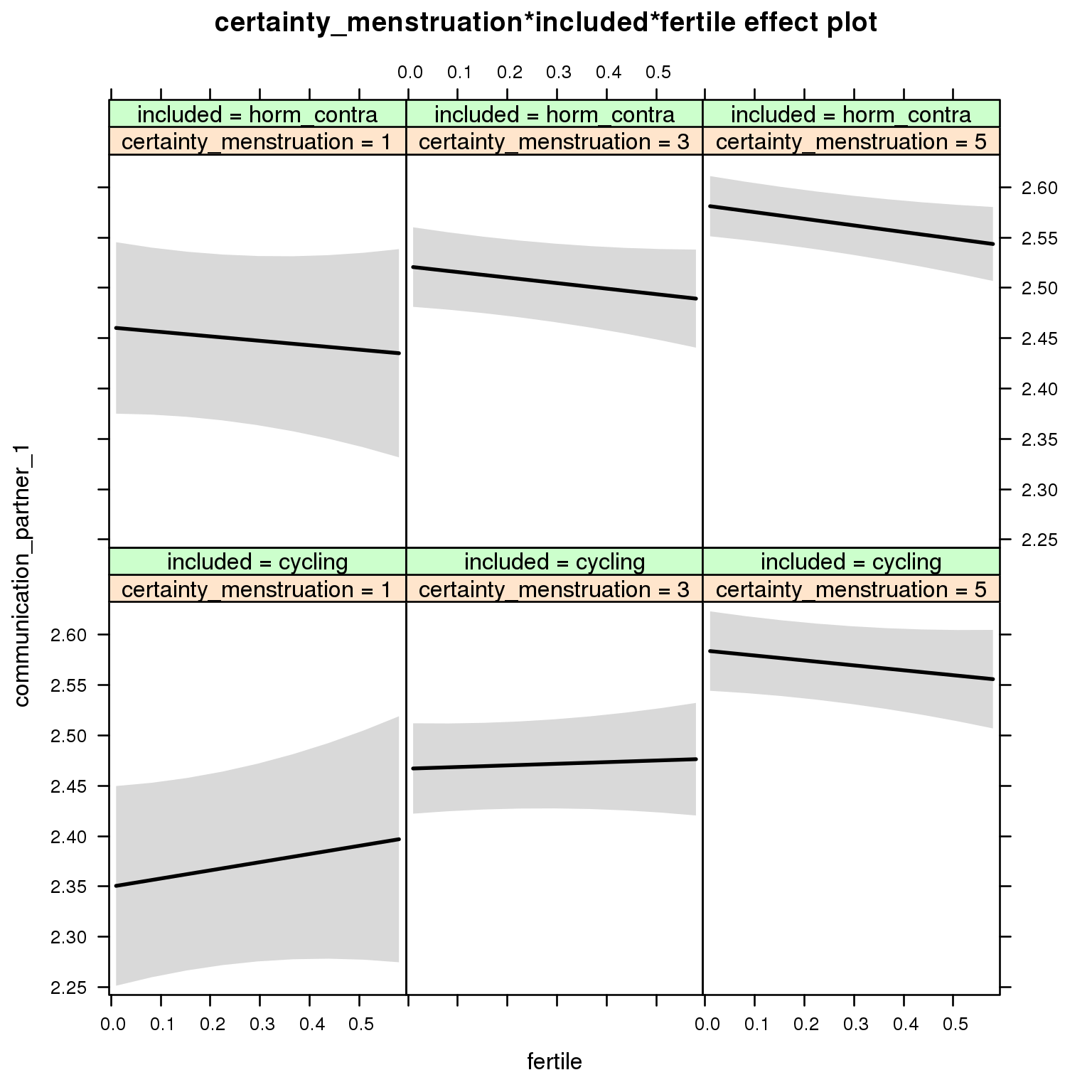
Linear mixed model fit by REML ['lmerMod']
Formula: communication_partner_1 ~ menstruation + fertile_mean + (1 |
person) + certainty_menstruation + included + fertile + menstruation:included +
certainty_menstruation:included + certainty_menstruation:fertile +
included:fertile + certainty_menstruation:included:fertile
Data: diary
REML criterion at convergence: 40852
Scaled residuals:
Min 1Q Median 3Q Max
-3.734 -0.848 0.250 0.785 2.909
Random effects:
Groups Name Variance Std.Dev.
person (Intercept) 0.0655 0.256
Residual 0.2505 0.501
Number of obs: 26704, groups: person, 1054
Fixed effects:
Estimate Std. Error t value
(Intercept) 2.31048 0.06847 33.7
menstruationpre 0.01768 0.01522 1.2
menstruationyes 0.00605 0.01433 0.4
fertile_mean -0.13556 0.11885 -1.1
certainty_menstruation 0.05863 0.01556 3.8
includedhorm_contra 0.15259 0.08681 1.8
fertile 0.11377 0.12079 0.9
menstruationpre:includedhorm_contra -0.04919 0.01953 -2.5
menstruationyes:includedhorm_contra -0.02694 0.01878 -1.4
certainty_menstruation:includedhorm_contra -0.02834 0.02016 -1.4
certainty_menstruation:fertile -0.03253 0.02830 -1.1
includedhorm_contra:fertile -0.15238 0.15689 -1.0
certainty_menstruation:includedhorm_contra:fertile 0.02709 0.03627 0.7
M_m8: Moderation by cycle regularity
model %>%
test_moderator("cycle_regularity", diary)refitting model(s) with ML (instead of REML)
| Df | AIC | BIC | logLik | deviance | Chisq | Chi Df | Pr(>Chisq) | |
|---|---|---|---|---|---|---|---|---|
| with_main | 15 | 40818 | 40941 | -20394 | 40788 | NA | NA | NA |
| with_mod | 19 | 40820 | 40975 | -20391 | 40782 | 6.731 | 4 | 0.1508 |
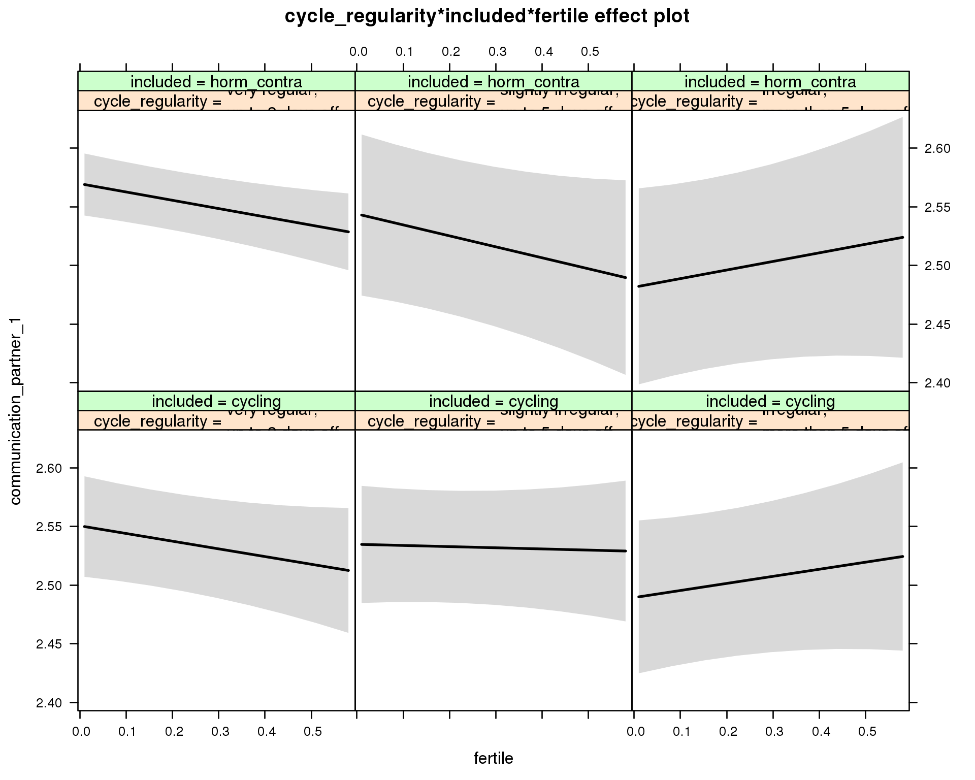
Linear mixed model fit by REML ['lmerMod']
Formula: communication_partner_1 ~ menstruation + fertile_mean + (1 |
person) + cycle_regularity + included + fertile + menstruation:included +
cycle_regularity:included + cycle_regularity:fertile + included:fertile +
cycle_regularity:included:fertile
Data: diary
REML criterion at convergence: 40870
Scaled residuals:
Min 1Q Median 3Q Max
-3.722 -0.849 0.248 0.788 2.918
Random effects:
Groups Name Variance Std.Dev.
person (Intercept) 0.0668 0.258
Residual 0.2505 0.501
Number of obs: 26704, groups: person, 1054
Fixed effects:
Estimate Std. Error t value
(Intercept) 2.56847 0.03011 85.3
menstruationpre 0.01697 0.01522 1.1
menstruationyes 0.00603 0.01432 0.4
fertile_mean -0.12628 0.11971 -1.1
cycle_regularityslightly irregular,\nup to 5 days off -0.01575 0.03347 -0.5
cycle_regularityirregular,\nmore than 5 days off -0.06114 0.03976 -1.5
includedhorm_contra 0.03262 0.02717 1.2
fertile -0.06558 0.04252 -1.5
menstruationpre:includedhorm_contra -0.04912 0.01954 -2.5
menstruationyes:includedhorm_contra -0.02775 0.01877 -1.5
cycle_regularityslightly irregular,\nup to 5 days off:includedhorm_contra -0.01003 0.05039 -0.2
cycle_regularityirregular,\nmore than 5 days off:includedhorm_contra -0.02704 0.05993 -0.5
cycle_regularityslightly irregular,\nup to 5 days off:fertile 0.05570 0.05858 1.0
cycle_regularityirregular,\nmore than 5 days off:fertile 0.12592 0.07197 1.7
includedhorm_contra:fertile -0.00513 0.04977 -0.1
cycle_regularityslightly irregular,\nup to 5 days off:includedhorm_contra:fertile -0.07845 0.08706 -0.9
cycle_regularityirregular,\nmore than 5 days off:includedhorm_contra:fertile 0.01800 0.10735 0.2
M_m9: Moderation by cohabitation status
model %>%
test_moderator("cohabitation", diary)refitting model(s) with ML (instead of REML)
| Df | AIC | BIC | logLik | deviance | Chisq | Chi Df | Pr(>Chisq) | |
|---|---|---|---|---|---|---|---|---|
| with_main | 15 | 40757 | 40880 | -20364 | 40727 | NA | NA | NA |
| with_mod | 19 | 40756 | 40912 | -20359 | 40718 | 8.67 | 4 | 0.06991 |
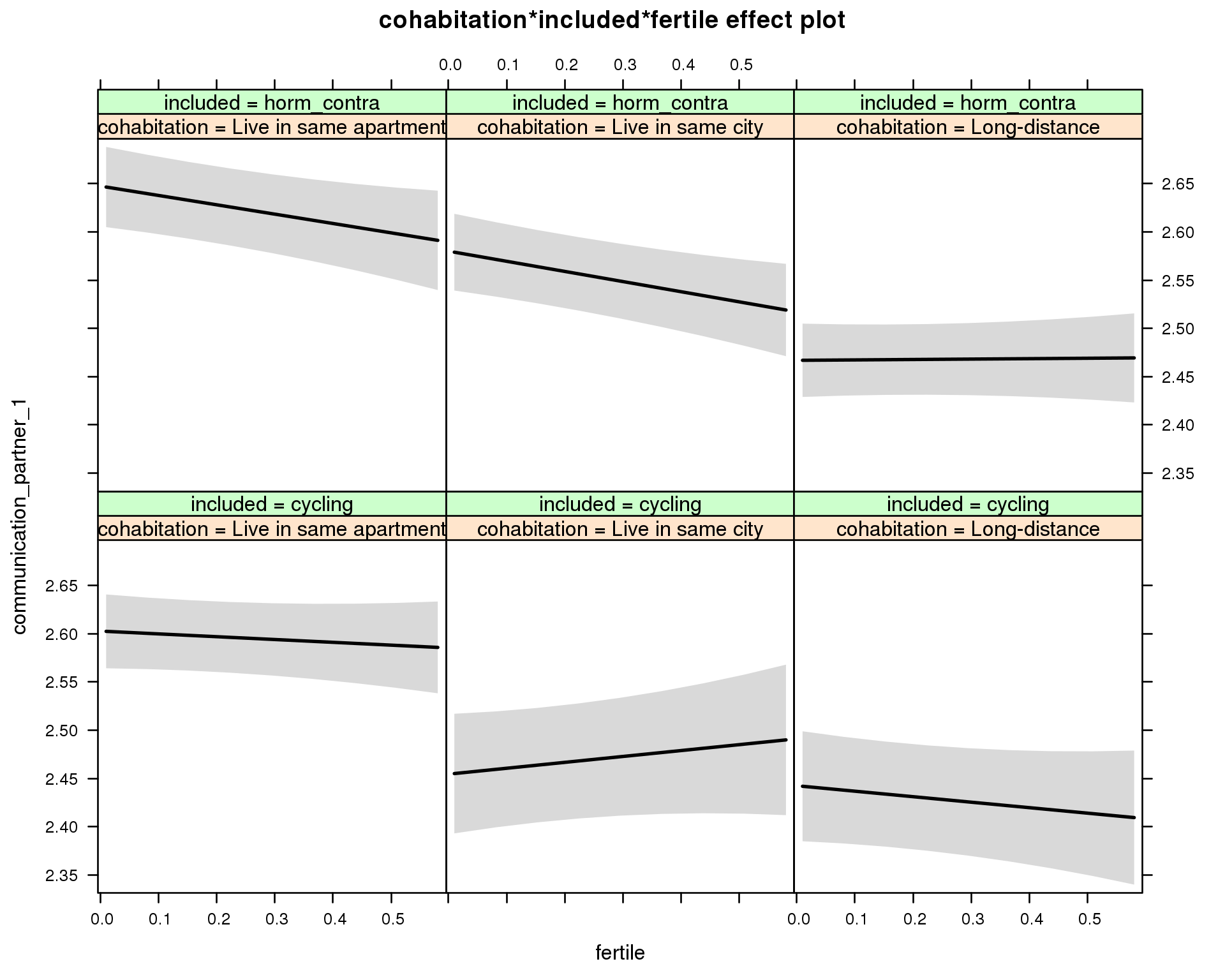
Linear mixed model fit by REML ['lmerMod']
Formula: communication_partner_1 ~ menstruation + fertile_mean + (1 |
person) + cohabitation + included + fertile + menstruation:included +
cohabitation:included + cohabitation:fertile + included:fertile + cohabitation:included:fertile
Data: diary
REML criterion at convergence: 40810
Scaled residuals:
Min 1Q Median 3Q Max
-3.714 -0.846 0.253 0.788 2.905
Random effects:
Groups Name Variance Std.Dev.
person (Intercept) 0.0621 0.249
Residual 0.2505 0.500
Number of obs: 26704, groups: person, 1054
Fixed effects:
Estimate Std. Error t value
(Intercept) 2.61813 0.02847 92.0
menstruationpre 0.01902 0.01520 1.3
menstruationyes 0.00794 0.01431 0.6
fertile_mean -0.11618 0.11681 -1.0
cohabitationLive in same city -0.14831 0.03714 -4.0
cohabitationLong-distance -0.16031 0.03500 -4.6
includedhorm_contra 0.05843 0.03008 1.9
fertile -0.02917 0.03837 -0.8
menstruationpre:includedhorm_contra -0.04917 0.01952 -2.5
menstruationyes:includedhorm_contra -0.02787 0.01875 -1.5
cohabitationLive in same city:includedhorm_contra 0.08086 0.04742 1.7
cohabitationLong-distance:includedhorm_contra -0.02029 0.04532 -0.4
cohabitationLive in same city:fertile 0.09039 0.06992 1.3
cohabitationLong-distance:fertile -0.02775 0.06303 -0.4
includedhorm_contra:fertile -0.06778 0.05597 -1.2
cohabitationLive in same city:includedhorm_contra:fertile -0.09860 0.08747 -1.1
cohabitationLong-distance:includedhorm_contra:fertile 0.12902 0.08124 1.6
M_m10: Moderation by relationship status
model %>%
test_moderator("relationship_status_clean", diary)refitting model(s) with ML (instead of REML)
| Df | AIC | BIC | logLik | deviance | Chisq | Chi Df | Pr(>Chisq) | |
|---|---|---|---|---|---|---|---|---|
| with_main | 15 | 40807 | 40930 | -20388 | 40777 | NA | NA | NA |
| with_mod | 19 | 40813 | 40969 | -20388 | 40775 | 1.967 | 4 | 0.7418 |
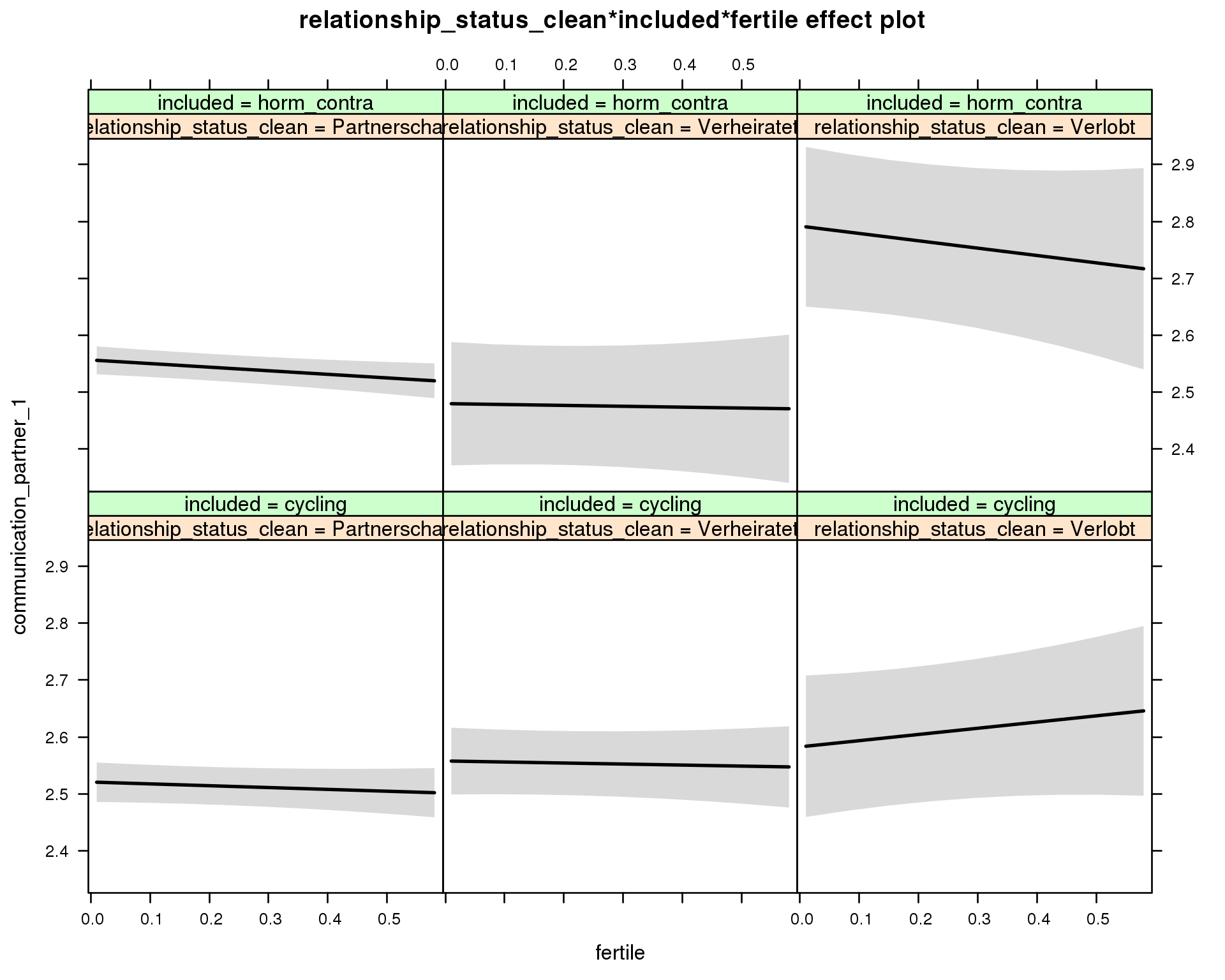
Linear mixed model fit by REML ['lmerMod']
Formula: communication_partner_1 ~ menstruation + fertile_mean + (1 |
person) + relationship_status_clean + included + fertile +
menstruation:included + relationship_status_clean:included +
relationship_status_clean:fertile + included:fertile + relationship_status_clean:included:fertile
Data: diary
REML criterion at convergence: 40857
Scaled residuals:
Min 1Q Median 3Q Max
-3.733 -0.847 0.248 0.786 2.915
Random effects:
Groups Name Variance Std.Dev.
person (Intercept) 0.0658 0.257
Residual 0.2506 0.501
Number of obs: 26704, groups: person, 1054
Fixed effects:
Estimate Std. Error t value
(Intercept) 2.53328 0.02718 93.2
menstruationpre 0.01826 0.01521 1.2
menstruationyes 0.00676 0.01431 0.5
fertile_mean -0.09658 0.11889 -0.8
relationship_status_cleanVerheiratet 0.03700 0.03472 1.1
relationship_status_cleanVerlobt 0.06181 0.06602 0.9
includedhorm_contra 0.04955 0.02332 2.1
fertile -0.03225 0.03515 -0.9
menstruationpre:includedhorm_contra -0.05022 0.01953 -2.6
menstruationyes:includedhorm_contra -0.02812 0.01876 -1.5
relationship_status_cleanVerheiratet:includedhorm_contra -0.11367 0.06666 -1.7
relationship_status_cleanVerlobt:includedhorm_contra 0.17339 0.09847 1.8
relationship_status_cleanVerheiratet:fertile 0.01429 0.06186 0.2
relationship_status_cleanVerlobt:fertile 0.14121 0.11588 1.2
includedhorm_contra:fertile -0.03076 0.04279 -0.7
relationship_status_cleanVerheiratet:includedhorm_contra:fertile 0.03320 0.11651 0.3
relationship_status_cleanVerlobt:includedhorm_contra:fertile -0.20728 0.18018 -1.2
Response time
Time of response
This model simply tests whether there was a main effect on time of response. Potentially, if participants delayed their responses more on (in)fertile days, they would have more behaviour to report on or could be more tired/hungry etc.
m_time_of_response = lmer(time_of_response ~ included * (menstruation + fertile) + fertile_mean + ( 1 | person), data = diary)
summary(m_time_of_response)## Linear mixed model fit by REML
## t-tests use Satterthwaite approximations to degrees of freedom ['lmerMod']
## Formula: time_of_response ~ included * (menstruation + fertile) + fertile_mean + (1 | person)
## Data: diary
##
## REML criterion at convergence: 115883
##
## Scaled residuals:
## Min 1Q Median 3Q Max
## -2.859 -0.778 -0.152 0.737 3.440
##
## Random effects:
## Groups Name Variance Std.Dev.
## person (Intercept) 0.81 0.90
## Residual 3.78 1.94
## Number of obs: 27357, groups: person, 1054
##
## Fixed effects:
## Estimate Std. Error df t value Pr(>|t|)
## (Intercept) 19.88910 0.09145 1759.00000 217.50 <2e-16 ***
## includedhorm_contra -0.10129 0.07581 1957.00000 -1.34 0.182
## menstruationpre 0.00608 0.05816 26984.00000 0.10 0.917
## menstruationyes -0.01549 0.05503 27109.00000 -0.28 0.778
## fertile 0.05937 0.11715 26934.00000 0.51 0.612
## fertile_mean 0.52583 0.42183 1823.00000 1.25 0.213
## includedhorm_contra:menstruationpre -0.03567 0.07470 26989.00000 -0.48 0.633
## includedhorm_contra:menstruationyes 0.00170 0.07222 27080.00000 0.02 0.981
## includedhorm_contra:fertile -0.34257 0.14822 27115.00000 -2.31 0.021 *
## ---
## Signif. codes: 0 '***' 0.001 '**' 0.01 '*' 0.05 '.' 0.1 ' ' 1
##
## Correlation of Fixed Effects:
## (Intr) incld_ mnstrtnp mnstrtny fertil frtl_m inclddhrm_cntr:mnstrtnp
## inclddhrm_c -0.483
## menstrutnpr -0.247 0.304
## menstrutnys -0.235 0.287 0.385
## fertile -0.235 0.375 0.461 0.376
## fertile_men -0.763 -0.029 -0.007 -0.005 -0.096
## inclddhrm_cntr:mnstrtnp 0.202 -0.381 -0.779 -0.300 -0.358 -0.007
## inclddhrm_cntr:mnstrtny 0.187 -0.354 -0.294 -0.762 -0.285 -0.007 0.372
## inclddhrm_cntr:f 0.235 -0.475 -0.364 -0.297 -0.784 0.012 0.461
## inclddhrm_cntr:mnstrtny
## inclddhrm_c
## menstrutnpr
## menstrutnys
## fertile
## fertile_men
## inclddhrm_cntr:mnstrtnp
## inclddhrm_cntr:mnstrtny
## inclddhrm_cntr:f 0.373Time taken for response
Here, we test if participants took longer to respond on fertile days. This is not necessarily a confound, as participants may take longer to fill out the survey because they are reporting more behaviours.
m_time_for_response = lmer(log10(time_for_response+1) ~ included * (menstruation + fertile) + fertile_mean + ( 1 | person), data = diary)
summary(m_time_for_response)## Linear mixed model fit by REML
## t-tests use Satterthwaite approximations to degrees of freedom ['lmerMod']
## Formula: log10(time_for_response + 1) ~ included * (menstruation + fertile) +
## fertile_mean + (1 | person)
## Data: diary
##
## REML criterion at convergence: -2050
##
## Scaled residuals:
## Min 1Q Median 3Q Max
## -3.472 -0.560 -0.217 0.263 6.727
##
## Random effects:
## Groups Name Variance Std.Dev.
## person (Intercept) 0.0113 0.106
## Residual 0.0503 0.224
## Number of obs: 26020, groups: person, 1053
##
## Fixed effects:
## Estimate Std. Error df t value Pr(>|t|)
## (Intercept) 0.73091 0.01098 1696.00000 66.55 <2e-16 ***
## includedhorm_contra -0.01183 0.00903 1888.00000 -1.31 0.1902
## menstruationpre 0.00319 0.00689 25624.00000 0.46 0.6436
## menstruationyes 0.01850 0.00650 25776.00000 2.85 0.0044 **
## fertile 0.01769 0.01391 25572.00000 1.27 0.2034
## fertile_mean 0.02387 0.05097 1746.00000 0.47 0.6396
## includedhorm_contra:menstruationpre -0.00787 0.00886 25628.00000 -0.89 0.3745
## includedhorm_contra:menstruationyes -0.00564 0.00852 25745.00000 -0.66 0.5079
## includedhorm_contra:fertile -0.02827 0.01760 25748.00000 -1.61 0.1083
## ---
## Signif. codes: 0 '***' 0.001 '**' 0.01 '*' 0.05 '.' 0.1 ' ' 1
##
## Correlation of Fixed Effects:
## (Intr) incld_ mnstrtnp mnstrtny fertil frtl_m inclddhrm_cntr:mnstrtnp
## inclddhrm_c -0.478
## menstrutnpr -0.249 0.309
## menstrutnys -0.239 0.294 0.392
## fertile -0.237 0.377 0.466 0.382
## fertile_men -0.767 -0.030 -0.005 -0.004 -0.093
## inclddhrm_cntr:mnstrtnp 0.203 -0.386 -0.778 -0.305 -0.362 -0.008
## inclddhrm_cntr:mnstrtny 0.190 -0.361 -0.299 -0.763 -0.291 -0.008 0.378
## inclddhrm_cntr:f 0.236 -0.478 -0.368 -0.302 -0.784 0.010 0.465
## inclddhrm_cntr:mnstrtny
## inclddhrm_c
## menstrutnpr
## menstrutnys
## fertile
## fertile_men
## inclddhrm_cntr:mnstrtnp
## inclddhrm_cntr:mnstrtny
## inclddhrm_cntr:f 0.379Time since last response
We asked participants to report on the last 24h or the time since their last diary entry. If women waited longer between entries on (in)fertile days, these could pose a problem. This does not appear to be the case.
m_time_since_last_response = lmer(time_since_last_response ~ included * (menstruation + fertile) + fertile_mean + ( 1 | person), data = diary)
summary(m_time_since_last_response)## Linear mixed model fit by REML
## t-tests use Satterthwaite approximations to degrees of freedom ['lmerMod']
## Formula: time_since_last_response ~ included * (menstruation + fertile) + fertile_mean + (1 | person)
## Data: diary
##
## REML criterion at convergence: 99556
##
## Scaled residuals:
## Min 1Q Median 3Q Max
## -2.6889 -0.5958 0.0078 0.5929 2.7214
##
## Random effects:
## Groups Name Variance Std.Dev.
## person (Intercept) 0.00 0.00
## Residual 6.69 2.59
## Number of obs: 21008, groups: person, 999
##
## Fixed effects:
## Estimate Std. Error df t value Pr(>|t|)
## (Intercept) 23.84674 0.07633 20999.00000 312.43 <2e-16 ***
## includedhorm_contra -0.00419 0.07076 20999.00000 -0.06 0.95
## menstruationpre 0.03782 0.08587 20999.00000 0.44 0.66
## menstruationyes 0.01446 0.08127 20999.00000 0.18 0.86
## fertile 0.11515 0.17504 20999.00000 0.66 0.51
## fertile_mean 0.29526 0.33812 20999.00000 0.87 0.38
## includedhorm_contra:menstruationpre -0.01826 0.11000 20999.00000 -0.17 0.87
## includedhorm_contra:menstruationyes -0.02246 0.10691 20999.00000 -0.21 0.83
## includedhorm_contra:fertile -0.10361 0.21868 20999.00000 -0.47 0.64
## ---
## Signif. codes: 0 '***' 0.001 '**' 0.01 '*' 0.05 '.' 0.1 ' ' 1
##
## Correlation of Fixed Effects:
## (Intr) incld_ mnstrtnp mnstrtny fertil frtl_m inclddhrm_cntr:mnstrtnp
## inclddhrm_c -0.549
## menstrutnpr -0.468 0.498
## menstrutnys -0.428 0.454 0.365
## fertile -0.424 0.597 0.462 0.368
## fertile_men -0.682 -0.041 0.009 0.011 -0.180
## inclddhrm_cntr:mnstrtnp 0.368 -0.624 -0.781 -0.285 -0.360 -0.011
## inclddhrm_cntr:mnstrtny 0.333 -0.559 -0.278 -0.760 -0.278 -0.019 0.352
## inclddhrm_cntr:f 0.427 -0.763 -0.371 -0.296 -0.777 0.015 0.467
## inclddhrm_cntr:mnstrtny
## inclddhrm_c
## menstrutnpr
## menstrutnys
## fertile
## fertile_men
## inclddhrm_cntr:mnstrtnp
## inclddhrm_cntr:mnstrtny
## inclddhrm_cntr:f 0.372Coefficient plot
library(broom)
coefs = models %>% lapply(FUN = tidy, conf.int = TRUE) %>%
bind_rows(.id = "outcome") %>%
select(-p.value) %>%
left_join(
models %>% lapply(FUN = get_p_val) %>%
bind_rows(.id = "outcome"),
by = c("outcome", "term")) %>%
mutate(outcome = factor(outcome),
term = factor(term),
group = factor(group),
p.value = pvalues(p.value))
coefs %>% filter(term %in% c("includedhorm_contra:fertile", "fertile")) %>%
ggplot(., aes(x = outcome, y = estimate, ymax = conf.high, ymin = conf.low, colour = term)) +
geom_hline(yintercept = 0, linetype = "dotted", color = "gray70") +
geom_text(aes(label = format(estimate, digits = 1, nsmall=2), y = estimate), vjust = -0.7,position = position_dodge(width = 0.6)) +
geom_pointrange( position = position_dodge(width = 0.6), size = 1) +
scale_color_manual("Contraception status", values = c("includedhorm_contra:fertile"="black","fertile" = "red"), labels = c("includedhorm_contra:fertile"="hormonally\ncontracepting","fertile" = "fertile"), guide = F) +
coord_flip()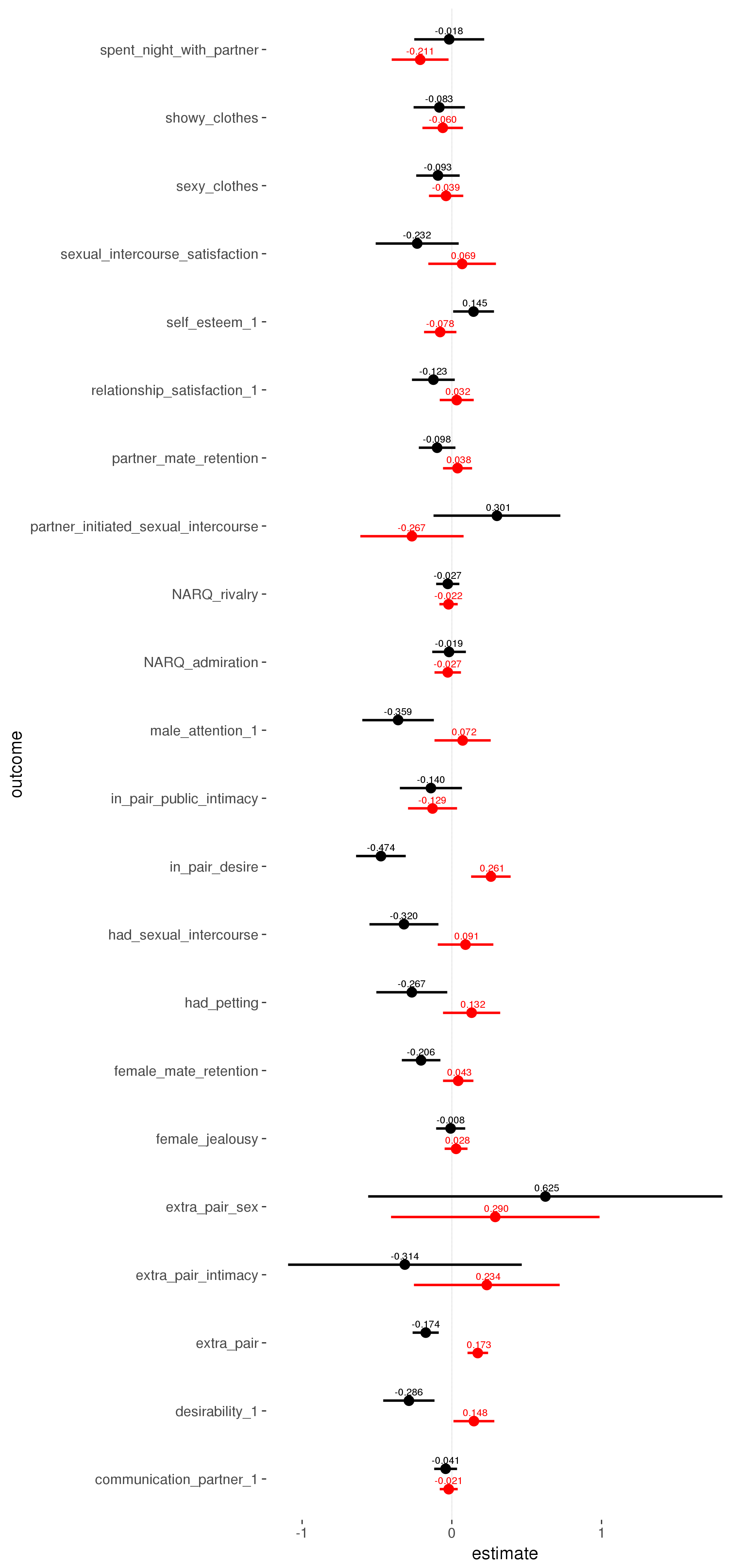
Table
library(DT)
coefs %>%
datatable(rownames = FALSE, filter = "top", extensions = 'Buttons', options = list(
dom = 'Bfrtip',
buttons = c('copy', 'csv', 'excel', 'pdf', 'print'),
pagelength = 20
)) %>%
formatRound(c("estimate", "std.error", "statistic", "conf.low", "conf.high"), 2)Wrap-up
saveRDS(models, file = "robustness_models.rds")