Compare effect sizes of ovulatory shifts in in- vs extra-pair desire
Cycling women (not on hormonal birth control)
Women on hormonal birth control
Theoretical background
Quoting from section 5.3. of our manuscript > More recent theoretical work emphasises that predictions of adaptive extra-pair sex, which Pillsworth and Haselton (2006a) call dual mating, should be divorced from predictions of ovulatory changes in mate preferences that do not necessarily precipitate extra-pair sex, but still function to bias sire choice (Gangestad, Thornhill, & Garver-Apgar, 2015). We cannot test all aspects of these recent theoretical developments in our study. An alternative, simpler explanation (Roney & Simmons, 2013) is based on life history theory. It suggests the observed increase in sexual desire during the fertile phase reflects a motivational priority change towards reproduction. The purported function would be to accept higher costs of sex (such as energetic and opportunity costs, or sexually transmitted infections), the more likely it is that sex leads to conception. This theory also predicts fertile phase drops in somatic investment, such as food intake (Fleischman & Fessler, 2007; Roney & Simmons, 2017). In this study, we did not assess any non-reproductive motivations, and we collected no data on single women. One theoretical perspective (Roney & Simmons, 2013) predicts a generalized increase in sex drive with fertility across the menstrual cycle, while others more specifically predict an increase in sexual interest for certain partners (e.g. Gangestad et al., 2015). These perspectives differ in predictions of whether the effect on extra-pair desire should be larger than that on in-pair desire.
Here, we document why we think it is not possible to discriminate between these two theoretical accounts in our data, nor is it wise to make conclusions about whether the effect on extra-pair desire is bigger than that on in-pair desire. The latter is unwise because we did not use parallel items to assess both desire, and did not assess single women. Effect sizes were descriptively similar and item-level comparisons hinted only that effects were larger on average for items that required no object of desire to be present and no action to be taken. Ultimately, as we show in a simple forward simulation here, without having measured general, target-unspecific, desire we cannot test whether general, target-unspecific sexual motivation drives the effects on in- and extra-pair desire we find (Roney, 2009).
The continuous backward-counted predictor recommended in (Gangestad et al., 2016) hedges for uncertainty in the estimation of the fertile window. Our effect sizes thus account for uncertainty and reflect the estimated change when certainly in the fertile window, although the predictor never gives a more confident prediction than 58%. In Likert points from 1 to 6, the fertile window effect was 0.26 [0.17;0.35] for extra-pair desire in the robustness check data. The in-pair desire effect had the same size: 0.26 [0.10;0.42]. We could now standardise the effects by the residual standard deviation in the multilevel model to obtain an effect size estimate similar to Cohen’s d. Since the residual standard deviation of extra-pair desire is much smaller (0.61) than that of in-pair desire (1.1), their standardised estimates then differ by a factor of two.
However, our items for in- and extra-pair desire were not comparable and upon inspecting item-level associations in Bayesian models that appropriately account for the ordinal nature of the Likert data, we believe comparisons between the two outcomes are futile. If we can conclude anything, effects were larger on average for items that required no object of desire to be present and no action to be taken. Future studies should attempt to settle the question of whether changes in extra- or in-pair desire are independent and different in size. Most importantly, they should test whether both can be simplified to an increase in sex drive that amplifies interest in all men without affecting their rank order, i.e. mate preferences. To do so, studies should construct parallel items to measure extra-pair, in-pair, and objectless sexual desire and behaviour, and test for fertile phase changes in the rank order of ratings of male stimuli.
Load data
# cd /usr/users/rarslan/relationship_dynamics/ && bsub -q mpi -W 48:00 -n 20 -R span[hosts=1] R -e "filebase = '3_fertility_robustness'; x = rmarkdown::render(paste0('3_fertility_robustness','.Rmd'), run_pandoc = FALSE, clean = FALSE); save(x, file = 'rob.rda'); cat(readLines(paste0(filebase,'.utf8.md')), sep = '\n')"
library(knitr)
opts_chunk$set(fig.width = 8, fig.height = 8, cache = T, warning = T, message = F, cache = F)
source("0_helpers.R")
load("full_data.rdata")
diary = diary %>%
mutate(
included = included_all,
fertile = prc_stirn_b_squished
) %>% group_by(person) %>%
mutate(
fertile_mean = mean(fertile, na.rm = T)
)
opts_chunk$set(warning = F)
library(Cairo)
opts_chunk$set(dev = "CairoPNG")
diary$age_group = cut(diary$age,c(18,20,25,30,35,70), include.lowest = T)models = list()
models$extra_pair_desire = lmer(extra_pair_desire ~ included * (menstruation + fertile) + fertile_mean + ( 1 | person), data = diary)
models$in_pair_desire = lmer(in_pair_desire ~ included * (menstruation + fertile) + fertile_mean + ( 1 | person), data = diary)
models$desirability_1 = lmer(desirability_1 ~ included * (menstruation + fertile) + fertile_mean + ( 1 | person), data = diary)Extra-pair desire
summary(models$extra_pair_desire)## Linear mixed model fit by REML
## t-tests use Satterthwaite approximations to degrees of freedom ['lmerMod']
## Formula: extra_pair_desire ~ included * (menstruation + fertile) + fertile_mean + (1 | person)
## Data: diary
##
## REML criterion at convergence: 34292
##
## Scaled residuals:
## Min 1Q Median 3Q Max
## -4.640 -0.486 -0.137 0.334 7.256
##
## Random effects:
## Groups Name Variance Std.Dev.
## person (Intercept) 0.379 0.616
## Residual 0.367 0.606
## Number of obs: 17321, groups: person, 819
##
## Fixed effects:
## Estimate Std. Error df t value Pr(>|t|)
## (Intercept) 1.8695 0.0599 969.0000 31.24 < 2e-16 ***
## includedhorm_contra -0.1980 0.0484 1031.0000 -4.09 0.0000461413 ***
## menstruationpre -0.1191 0.0201 16661.0000 -5.92 0.0000000034 ***
## menstruationyes -0.0821 0.0237 16636.0000 -3.46 0.00054 ***
## fertile 0.2570 0.0458 16592.0000 5.61 0.0000000209 ***
## fertile_mean -0.8057 0.3120 895.0000 -2.58 0.00997 **
## includedhorm_contra:menstruationpre 0.0900 0.0263 16670.0000 3.42 0.00063 ***
## includedhorm_contra:menstruationyes 0.0903 0.0332 16633.0000 2.72 0.00659 **
## includedhorm_contra:fertile -0.1887 0.0606 16628.0000 -3.11 0.00186 **
## ---
## Signif. codes: 0 '***' 0.001 '**' 0.01 '*' 0.05 '.' 0.1 ' ' 1
##
## Correlation of Fixed Effects:
## (Intr) incld_ mnstrtnp mnstrtny fertil frtl_m inclddhrm_cntr:mnstrtnp
## inclddhrm_c -0.478
## menstrutnpr -0.193 0.219
## menstrutnys -0.118 0.148 0.361
## fertile -0.156 0.225 0.513 0.322
## fertile_men -0.781 -0.006 0.020 -0.002 -0.033
## inclddhrm_cntr:mnstrtnp 0.135 -0.294 -0.765 -0.276 -0.393 0.002
## inclddhrm_cntr:mnstrtny 0.085 -0.188 -0.258 -0.714 -0.230 0.001 0.350
## inclddhrm_cntr:f 0.139 -0.300 -0.388 -0.244 -0.755 -0.002 0.525
## inclddhrm_cntr:mnstrtny
## inclddhrm_c
## menstrutnpr
## menstrutnys
## fertile
## fertile_men
## inclddhrm_cntr:mnstrtnp
## inclddhrm_cntr:mnstrtny
## inclddhrm_cntr:f 0.319In-pair desire
summary(models$in_pair_desire)## Linear mixed model fit by REML
## t-tests use Satterthwaite approximations to degrees of freedom ['lmerMod']
## Formula: in_pair_desire ~ included * (menstruation + fertile) + fertile_mean + (1 | person)
## Data: diary
##
## REML criterion at convergence: 54220
##
## Scaled residuals:
## Min 1Q Median 3Q Max
## -3.406 -0.683 -0.033 0.664 3.509
##
## Random effects:
## Groups Name Variance Std.Dev.
## person (Intercept) 0.717 0.847
## Residual 1.188 1.090
## Number of obs: 17321, groups: person, 819
##
## Fixed effects:
## Estimate Std. Error df t value Pr(>|t|)
## (Intercept) 3.4623 0.0862 1061.0000 40.15 < 2e-16 ***
## includedhorm_contra 0.2492 0.0704 1196.0000 3.54 0.00042 ***
## menstruationpre -0.0685 0.0362 16746.0000 -1.89 0.05820 .
## menstruationyes -0.1469 0.0426 16733.0000 -3.45 0.00057 ***
## fertile 0.2557 0.0824 16662.0000 3.10 0.00191 **
## fertile_mean 0.2957 0.4445 942.0000 0.67 0.50608
## includedhorm_contra:menstruationpre 0.0372 0.0473 16754.0000 0.79 0.43080
## includedhorm_contra:menstruationyes 0.0907 0.0597 16728.0000 1.52 0.12842
## includedhorm_contra:fertile -0.3562 0.1089 16718.0000 -3.27 0.00108 **
## ---
## Signif. codes: 0 '***' 0.001 '**' 0.01 '*' 0.05 '.' 0.1 ' ' 1
##
## Correlation of Fixed Effects:
## (Intr) incld_ mnstrtnp mnstrtny fertil frtl_m inclddhrm_cntr:mnstrtnp
## inclddhrm_c -0.480
## menstrutnpr -0.238 0.269
## menstrutnys -0.148 0.183 0.361
## fertile -0.194 0.278 0.514 0.322
## fertile_men -0.777 -0.006 0.023 -0.003 -0.043
## inclddhrm_cntr:mnstrtnp 0.167 -0.361 -0.765 -0.276 -0.394 0.002
## inclddhrm_cntr:mnstrtny 0.106 -0.232 -0.258 -0.714 -0.230 0.001 0.350
## inclddhrm_cntr:f 0.173 -0.371 -0.389 -0.243 -0.755 -0.002 0.526
## inclddhrm_cntr:mnstrtny
## inclddhrm_c
## menstrutnpr
## menstrutnys
## fertile
## fertile_men
## inclddhrm_cntr:mnstrtnp
## inclddhrm_cntr:mnstrtny
## inclddhrm_cntr:f 0.319Desirability
summary(models$desirability_1)## Linear mixed model fit by REML
## t-tests use Satterthwaite approximations to degrees of freedom ['lmerMod']
## Formula: desirability_1 ~ included * (menstruation + fertile) + fertile_mean + (1 | person)
## Data: diary
##
## REML criterion at convergence: 55270
##
## Scaled residuals:
## Min 1Q Median 3Q Max
## -4.035 -0.612 0.035 0.664 3.415
##
## Random effects:
## Groups Name Variance Std.Dev.
## person (Intercept) 0.688 0.83
## Residual 1.267 1.13
## Number of obs: 17325, groups: person, 819
##
## Fixed effects:
## Estimate Std. Error df t value Pr(>|t|)
## (Intercept) 3.7277 0.0854 1078.0000 43.62 < 2e-16 ***
## includedhorm_contra -0.0094 0.0699 1234.0000 -0.13 0.8931
## menstruationpre -0.1121 0.0373 16767.0000 -3.00 0.0027 **
## menstruationyes -0.2418 0.0440 16758.0000 -5.49 0.00000004 ***
## fertile 0.1402 0.0850 16680.0000 1.65 0.0992 .
## fertile_mean 0.0931 0.4393 949.0000 0.21 0.8323
## includedhorm_contra:menstruationpre 0.0535 0.0488 16774.0000 1.10 0.2725
## includedhorm_contra:menstruationyes 0.1079 0.0616 16752.0000 1.75 0.0799 .
## includedhorm_contra:fertile -0.1983 0.1124 16740.0000 -1.76 0.0777 .
## ---
## Signif. codes: 0 '***' 0.001 '**' 0.01 '*' 0.05 '.' 0.1 ' ' 1
##
## Correlation of Fixed Effects:
## (Intr) incld_ mnstrtnp mnstrtny fertil frtl_m inclddhrm_cntr:mnstrtnp
## inclddhrm_c -0.481
## menstrutnpr -0.248 0.280
## menstrutnys -0.154 0.191 0.361
## fertile -0.202 0.289 0.514 0.322
## fertile_men -0.776 -0.006 0.024 -0.003 -0.045
## inclddhrm_cntr:mnstrtnp 0.174 -0.374 -0.765 -0.276 -0.394 0.002
## inclddhrm_cntr:mnstrtny 0.111 -0.241 -0.258 -0.715 -0.230 0.001 0.350
## inclddhrm_cntr:f 0.181 -0.386 -0.389 -0.243 -0.755 -0.002 0.526
## inclddhrm_cntr:mnstrtny
## inclddhrm_c
## menstrutnpr
## menstrutnys
## fertile
## fertile_men
## inclddhrm_cntr:mnstrtnp
## inclddhrm_cntr:mnstrtny
## inclddhrm_cntr:f 0.319Comparison
Here, we compare both the standardised and unstandardised effect sizes of extra-pair and in-pair desire. As we did not predict a difference, we merely test whether the estimates fall into the 95% confidence intervals of one another. Standardisation is done by dividing by the residual standard deviation.
- Standardised, extra-pair desire: 0.42 [0.28;0.57].
- Unstandardised, extra-pair desire: 0.26 [0.17;0.35].
- Standardised, in-pair desire: 0.23 [0.09;0.38].
- Unstandardised, in-pair desire: 0.26 [0.09;0.42].
- Standardised, desirability: 0.12 [-0.02;0.27].
- Unstandardised, desirability: 0.14 [-0.03;0.31].
By item
items_engl = xlsx::read.xlsx("item_tables/Daily_items_bearbeitetAM.xlsx", 1)
library(brms)
c('extra_pair_7', 'extra_pair_10', 'extra_pair_11', 'extra_pair_12', 'extra_pair_13', 'sexual_intercourse_1', 'desirability_partner', 'attention_2') %>%
  lapply(FUN = function(x) {
    paste0("by_item/", x , ".rds") %>%
    readRDS() ->
      fit
    samples = fit %>% posterior_samples("^b_fertile$") %>%  mutate(item = x)
    newd = data.frame(person = NA, included = "cycling", fertile_mean = 0.1, menstruation = "no", fertile = c(0.01,0.51))
    predicted = fitted(fit, newdata = newd, summary = FALSE, re_formula = NA, allow_new_levels = F)
    predicted_sum = fitted(fit, newdata = newd, summary = T)
    #dims: 4000 samples, 2 rows, 6 levels
    multiply_by_level = rep(sort(unique(fit$data[,1])), each = dim(predicted)[1] * dim(predicted)[2]) # repeat each as many times as the first two dims
    dim(multiply_by_level) = dim(predicted)
    predicted = predicted * multiply_by_level
    response = apply(predicted, MARGIN = c(1:2), FUN = sum)
    effect = response[,2] - response[,1]
    samples$effect = effect
    samples
}) %>% bind_rows() -> post_samples

post_samples = post_samples %>%
  mutate(effect = if_else(item == "sexual_intercourse_1", effect/5*6, effect)) %>%
  mutate(in_pair = !item %contains% "extra") %>%
  group_by(in_pair) %>%
  left_join(items_engl %>% select(Item.name, Item), by = c("item" = "Item.name"))

post_samples %>%
  summarise_at(c("b_fertile", "effect"),
               funs(mean = mean(.), ci_lo = quantile(., probs = 0.025), ci_hi = quantile(., probs = 0.975))) %>%
pander()| in_pair | b_fertile_mean | effect_mean | b_fertile_ci_lo | effect_ci_lo | b_fertile_ci_hi | effect_ci_hi |
|---|---|---|---|---|---|---|
| FALSE | 0.511 | 0.08452 | 0.00772 | 0.0007318 | 1.027 | 0.2622 |
| TRUE | 0.4162 | 0.1446 | 0.07387 | 0.02708 | 0.7917 | 0.2664 |
post_samples %>%
  mutate(Item = str_wrap(Item, 35)) %>%
  ggplot(aes(x = effect, y = Item, fill = in_pair)) +
  ggjoy::geom_joy(panel_scaling = T, color = "white") +
  scale_fill_brewer()  + ggjoy::theme_joy()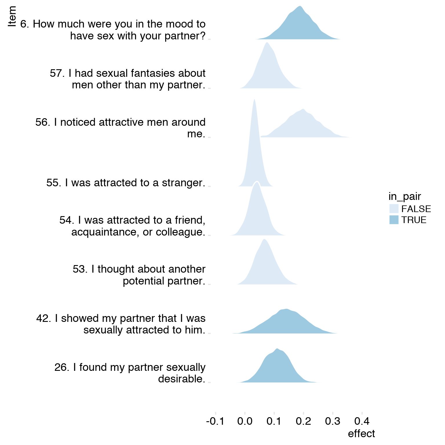
Forward-simulate generalized sexual desire
Because we had not collected information on undirected sexual desire, we found it difficult to determine whether the effects of the fertile window on extra- vs. in-pair desire were independent or manifestations of the same generalized desire applied to different objects. See also effect size comparison.
Forward-simulation, scenario 1, generalized desire
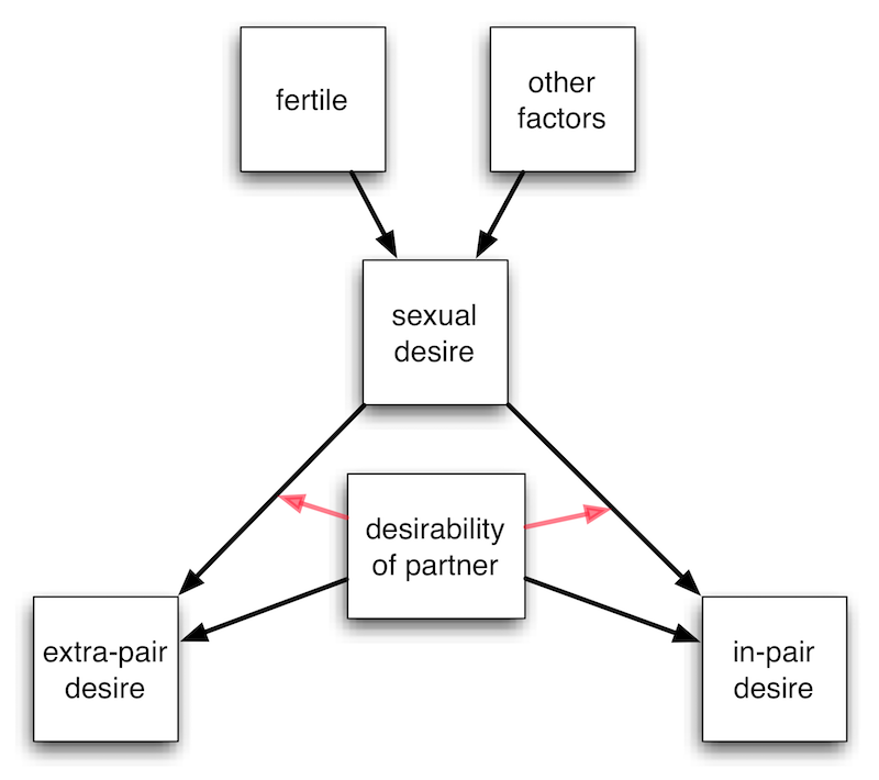
Here, we simulate 500 women, measured on 30 days each. The fertile window only has an effect on generalized desire (henceforth “sexual desire”). For women whose partners is suitable (crosses the threshold of 0) object of sexual fantasies, sexual desire translates into in-pair desire, for others into extra-pair desire. We graphed a potential causal model below (in red: moderator arrows on the arrows between sexual desire and EP/IP desire as commonly done in psychology). See also this directed acyclic graph in DAGitty.
set.seed(5564)
source('0_helpers.R')
library(effects)
library(lme4)

yn = c(0,1)
n_person = 500
days = 30
n = n_person * days
persons = data_frame(
  person = 1:n_person,
  basic_sexual_desire = rnorm(n_person),
  desirability_of_partner = rnorm(n_person),
  desirability_of_partner_m = rnorm(n_person) + rnorm(n_person) / 3
)
sim = data_frame(
  person = rep(1:500, each = days),
    fertile = sample(yn, size = n, replace = T, prob = c(0.7, 0.3))
) %>%
  full_join(persons, by = 'person') %>%
mutate(
    sexual_desire = basic_sexual_desire/2  + rnorm(n)/2 + 1 * fertile,
    ep_desire = rnorm(n) + sexual_desire * ifelse(desirability_of_partner < 0, 1, 0) + -1 * desirability_of_partner,
    ip_desire = rnorm(n) + sexual_desire * ifelse(desirability_of_partner > 0, 1, 0) + desirability_of_partner
)
Unobserved patterns
In our data, we cannot run this test, which shows that the effect of fertile on EP/IP desire is mediated completely by sexual desire
summary(lmer(sexual_desire ~ fertile + (1 | person), sim)) # not seen## Linear mixed model fit by REML
## t-tests use Satterthwaite approximations to degrees of freedom ['lmerMod']
## Formula: sexual_desire ~ fertile + (1 | person)
## Data: sim
##
## REML criterion at convergence: 23721
##
## Scaled residuals:
## Min 1Q Median 3Q Max
## -3.689 -0.662 -0.004 0.666 3.584
##
## Random effects:
## Groups Name Variance Std.Dev.
## person (Intercept) 0.231 0.481
## Residual 0.254 0.504
## Number of obs: 15000, groups: person, 500
##
## Fixed effects:
## Estimate Std. Error df t value Pr(>|t|)
## (Intercept) -0.0647 0.0221 515.0000 -2.93 0.0035 **
## fertile 1.0056 0.0091 14534.0000 110.48 <2e-16 ***
## ---
## Signif. codes: 0 '***' 0.001 '**' 0.01 '*' 0.05 '.' 0.1 ' ' 1
##
## Correlation of Fixed Effects:
## (Intr)
## fertile -0.125summary(lmer(ip_desire ~ sexual_desire + fertile + (1 | person), sim)) # not seen## Linear mixed model fit by REML
## t-tests use Satterthwaite approximations to degrees of freedom ['lmerMod']
## Formula: ip_desire ~ sexual_desire + fertile + (1 | person)
## Data: sim
##
## REML criterion at convergence: 46123
##
## Scaled residuals:
## Min 1Q Median 3Q Max
## -3.661 -0.657 0.004 0.662 3.873
##
## Random effects:
## Groups Name Variance Std.Dev.
## person (Intercept) 1.18 1.09
## Residual 1.13 1.06
## Number of obs: 15000, groups: person, 500
##
## Fixed effects:
## Estimate Std. Error df t value Pr(>|t|)
## (Intercept) 0.03350 0.04969 514.00000 0.67 0.50
## sexual_desire 0.49127 0.01723 14989.00000 28.52 <2e-16 ***
## fertile -0.00716 0.02583 14821.00000 -0.28 0.78
## ---
## Signif. codes: 0 '***' 0.001 '**' 0.01 '*' 0.05 '.' 0.1 ' ' 1
##
## Correlation of Fixed Effects:
## (Intr) sxl_ds
## sexual_desr 0.022
## fertile -0.102 -0.671summary(lmer(ep_desire ~ sexual_desire + fertile + (1 | person), sim)) # not seen## Linear mixed model fit by REML
## t-tests use Satterthwaite approximations to degrees of freedom ['lmerMod']
## Formula: ep_desire ~ sexual_desire + fertile + (1 | person)
## Data: sim
##
## REML criterion at convergence: 46298
##
## Scaled residuals:
## Min 1Q Median 3Q Max
## -3.791 -0.670 0.004 0.671 4.205
##
## Random effects:
## Groups Name Variance Std.Dev.
## person (Intercept) 1.19 1.09
## Residual 1.14 1.07
## Number of obs: 15000, groups: person, 500
##
## Fixed effects:
## Estimate Std. Error df t value Pr(>|t|)
## (Intercept) -0.01121 0.04994 514.00000 -0.22 0.82
## sexual_desire 0.48818 0.01733 14989.00000 28.17 <2e-16 ***
## fertile 0.00291 0.02598 14821.00000 0.11 0.91
## ---
## Signif. codes: 0 '***' 0.001 '**' 0.01 '*' 0.05 '.' 0.1 ' ' 1
##
## Correlation of Fixed Effects:
## (Intr) sxl_ds
## sexual_desr 0.022
## fertile -0.102 -0.671summary(lmer(ep_desire ~ fertile + sexual_desire * desirability_of_partner_m + (1 | person), sim)) # not seen## Linear mixed model fit by REML
## t-tests use Satterthwaite approximations to degrees of freedom ['lmerMod']
## Formula: ep_desire ~ fertile + sexual_desire * desirability_of_partner_m + (1 | person)
## Data: sim
##
## REML criterion at convergence: 46297
##
## Scaled residuals:
## Min 1Q Median 3Q Max
## -3.785 -0.671 0.005 0.673 4.205
##
## Random effects:
## Groups Name Variance Std.Dev.
## person (Intercept) 1.19 1.09
## Residual 1.14 1.07
## Number of obs: 15000, groups: person, 500
##
## Fixed effects:
## Estimate Std. Error df t value Pr(>|t|)
## (Intercept) -0.00817 0.04994 513.00000 -0.16 0.8700
## fertile 0.00363 0.02598 14821.00000 0.14 0.8889
## sexual_desire 0.48956 0.01733 14988.00000 28.25 <2e-16 ***
## desirability_of_partner_m 0.05979 0.04761 501.00000 1.26 0.2098
## sexual_desire:desirability_of_partner_m 0.04014 0.01242 14873.00000 3.23 0.0012 **
## ---
## Signif. codes: 0 '***' 0.001 '**' 0.01 '*' 0.05 '.' 0.1 ' ' 1
##
## Correlation of Fixed Effects:
## (Intr) fertil sxl_ds dsr___
## fertile -0.102
## sexual_desr 0.022 -0.670
## dsrblty_f__ 0.056 -0.001 -0.004
## sxl_dsr:___ -0.006 0.009 0.026 -0.057summary(lmer(ip_desire ~ fertile + sexual_desire * desirability_of_partner_m + (1 | person), sim)) # not seen## Linear mixed model fit by REML
## t-tests use Satterthwaite approximations to degrees of freedom ['lmerMod']
## Formula: ip_desire ~ fertile + sexual_desire * desirability_of_partner_m + (1 | person)
## Data: sim
##
## REML criterion at convergence: 46123
##
## Scaled residuals:
## Min 1Q Median 3Q Max
## -3.659 -0.659 0.007 0.663 3.912
##
## Random effects:
## Groups Name Variance Std.Dev.
## person (Intercept) 1.18 1.08
## Residual 1.13 1.06
## Number of obs: 15000, groups: person, 500
##
## Fixed effects:
## Estimate Std. Error df t value Pr(>|t|)
## (Intercept) 0.03022 0.04968 513.00000 0.61 0.5433
## fertile -0.00781 0.02583 14820.00000 -0.30 0.7625
## sexual_desire 0.49002 0.01723 14988.00000 28.45 <2e-16 ***
## desirability_of_partner_m -0.06335 0.04737 501.00000 -1.34 0.1817
## sexual_desire:desirability_of_partner_m -0.03635 0.01235 14873.00000 -2.94 0.0032 **
## ---
## Signif. codes: 0 '***' 0.001 '**' 0.01 '*' 0.05 '.' 0.1 ' ' 1
##
## Correlation of Fixed Effects:
## (Intr) fertil sxl_ds dsr___
## fertile -0.102
## sexual_desr 0.022 -0.670
## dsrblty_f__ 0.056 -0.001 -0.004
## sxl_dsr:___ -0.006 0.009 0.026 -0.057Observed patterns
We can observe the main effects of the fertile window.
summary(lmer(ep_desire ~ fertile + (1 | person), sim)) # seen## Linear mixed model fit by REML
## t-tests use Satterthwaite approximations to degrees of freedom ['lmerMod']
## Formula: ep_desire ~ fertile + (1 | person)
## Data: sim
##
## REML criterion at convergence: 47065
##
## Scaled residuals:
## Min 1Q Median 3Q Max
## -4.068 -0.669 0.003 0.656 4.496
##
## Random effects:
## Groups Name Variance Std.Dev.
## person (Intercept) 1.25 1.12
## Residual 1.20 1.10
## Number of obs: 15000, groups: person, 500
##
## Fixed effects:
## Estimate Std. Error df t value Pr(>|t|)
## (Intercept) -0.0428 0.0512 513.0000 -0.84 0.4
## fertile 0.4938 0.0198 14530.0000 24.97 <2e-16 ***
## ---
## Signif. codes: 0 '***' 0.001 '**' 0.01 '*' 0.05 '.' 0.1 ' ' 1
##
## Correlation of Fixed Effects:
## (Intr)
## fertile -0.118summary(lmer(ip_desire ~ fertile + (1 | person), sim)) # seen## Linear mixed model fit by REML
## t-tests use Satterthwaite approximations to degrees of freedom ['lmerMod']
## Formula: ip_desire ~ fertile + (1 | person)
## Data: sim
##
## REML criterion at convergence: 46909
##
## Scaled residuals:
## Min 1Q Median 3Q Max
## -3.836 -0.666 0.001 0.648 4.080
##
## Random effects:
## Groups Name Variance Std.Dev.
## person (Intercept) 1.23 1.11
## Residual 1.19 1.09
## Number of obs: 15000, groups: person, 500
##
## Fixed effects:
## Estimate Std. Error df t value Pr(>|t|)
## (Intercept) 0.00171 0.05074 513.00000 0.03 0.97
## fertile 0.48684 0.01968 14530.00000 24.74 <2e-16 ***
## ---
## Signif. codes: 0 '***' 0.001 '**' 0.01 '*' 0.05 '.' 0.1 ' ' 1
##
## Correlation of Fixed Effects:
## (Intr)
## fertile -0.118We ran the following analyses to test whether the effects were independent.
summary(lmer(ip_desire ~ ep_desire + fertile + (1 | person), sim)) # doable## Linear mixed model fit by REML
## t-tests use Satterthwaite approximations to degrees of freedom ['lmerMod']
## Formula: ip_desire ~ ep_desire + fertile + (1 | person)
## Data: sim
##
## REML criterion at convergence: 46836
##
## Scaled residuals:
## Min 1Q Median 3Q Max
## -3.751 -0.669 0.004 0.656 4.154
##
## Random effects:
## Groups Name Variance Std.Dev.
## person (Intercept) 1.07 1.03
## Residual 1.19 1.09
## Number of obs: 15000, groups: person, 500
##
## Fixed effects:
## Estimate Std. Error df t value Pr(>|t|)
## (Intercept) -0.00147 0.04745 486.00000 -0.03 0.98
## ep_desire -0.07485 0.00810 14985.00000 -9.24 <2e-16 ***
## fertile 0.52374 0.02007 14547.00000 26.09 <2e-16 ***
## ---
## Signif. codes: 0 '***' 0.001 '**' 0.01 '*' 0.05 '.' 0.1 ' ' 1
##
## Correlation of Fixed Effects:
## (Intr) ep_dsr
## ep_desire 0.007
## fertile -0.125 -0.199summary(lmer(ep_desire ~ ip_desire + fertile + (1 | person), sim)) # doable## Linear mixed model fit by REML
## t-tests use Satterthwaite approximations to degrees of freedom ['lmerMod']
## Formula: ep_desire ~ ip_desire + fertile + (1 | person)
## Data: sim
##
## REML criterion at convergence: 46993
##
## Scaled residuals:
## Min 1Q Median 3Q Max
## -4.031 -0.663 0.008 0.658 4.620
##
## Random effects:
## Groups Name Variance Std.Dev.
## person (Intercept) 1.09 1.04
## Residual 1.20 1.10
## Number of obs: 15000, groups: person, 500
##
## Fixed effects:
## Estimate Std. Error df t value Pr(>|t|)
## (Intercept) -0.04268 0.04790 486.00000 -0.89 0.37
## ip_desire -0.07536 0.00819 14988.00000 -9.21 <2e-16 ***
## fertile 0.53053 0.02017 14549.00000 26.31 <2e-16 ***
## ---
## Signif. codes: 0 '***' 0.001 '**' 0.01 '*' 0.05 '.' 0.1 ' ' 1
##
## Correlation of Fixed Effects:
## (Intr) ip_dsr
## ip_desire 0.000
## fertile -0.123 -0.198summary(lmer(ep_desire ~ fertile * ip_desire + (1 | person), sim)) # doable## Linear mixed model fit by REML
## t-tests use Satterthwaite approximations to degrees of freedom ['lmerMod']
## Formula: ep_desire ~ fertile * ip_desire + (1 | person)
## Data: sim
##
## REML criterion at convergence: 46737
##
## Scaled residuals:
## Min 1Q Median 3Q Max
## -4.069 -0.660 0.001 0.662 4.805
##
## Random effects:
## Groups Name Variance Std.Dev.
## person (Intercept) 1.10 1.05
## Residual 1.18 1.09
## Number of obs: 15000, groups: person, 500
##
## Fixed effects:
## Estimate Std. Error df t value Pr(>|t|)
## (Intercept) -0.04302 0.04802 486.00000 -0.90 0.37
## fertile 0.58615 0.02028 14544.00000 28.91 <2e-16 ***
## ip_desire 0.00323 0.00942 14985.00000 0.34 0.73
## fertile:ip_desire -0.19428 0.01193 14514.00000 -16.28 <2e-16 ***
## ---
## Signif. codes: 0 '***' 0.001 '**' 0.01 '*' 0.05 '.' 0.1 ' ' 1
##
## Correlation of Fixed Effects:
## (Intr) fertil ip_dsr
## fertile -0.120
## ip_desire 0.000 -0.082
## fertl:p_dsr 0.000 -0.170 -0.508summary(lmer(ip_desire ~ fertile * ep_desire + (1 | person), sim)) # doable## Linear mixed model fit by REML
## t-tests use Satterthwaite approximations to degrees of freedom ['lmerMod']
## Formula: ip_desire ~ fertile * ep_desire + (1 | person)
## Data: sim
##
## REML criterion at convergence: 46598
##
## Scaled residuals:
## Min 1Q Median 3Q Max
## -3.738 -0.669 0.004 0.646 4.235
##
## Random effects:
## Groups Name Variance Std.Dev.
## person (Intercept) 1.07 1.04
## Residual 1.17 1.08
## Number of obs: 15000, groups: person, 500
##
## Fixed effects:
## Estimate Std. Error df t value Pr(>|t|)
## (Intercept) 0.001696 0.047564 486.000000 0.04 0.97
## fertile 0.571269 0.020133 14543.000000 28.37 <2e-16 ***
## ep_desire 0.000716 0.009342 14988.000000 0.08 0.94
## fertile:ep_desire -0.185176 0.011784 14514.000000 -15.71 <2e-16 ***
## ---
## Signif. codes: 0 '***' 0.001 '**' 0.01 '*' 0.05 '.' 0.1 ' ' 1
##
## Correlation of Fixed Effects:
## (Intr) fertil ep_dsr
## fertile -0.122
## ep_desire 0.008 -0.092
## fertl:p_dsr -0.004 -0.151 -0.510# doable in theory, if we knew the moderator
summary(lmer(ep_desire ~ fertile + desirability_of_partner_m * ip_desire + (1 | person), sim))## Linear mixed model fit by REML
## t-tests use Satterthwaite approximations to degrees of freedom ['lmerMod']
## Formula: ep_desire ~ fertile + desirability_of_partner_m * ip_desire + (1 | person)
## Data: sim
##
## REML criterion at convergence: 47003
##
## Scaled residuals:
## Min 1Q Median 3Q Max
## -4.030 -0.664 0.007 0.657 4.606
##
## Random effects:
## Groups Name Variance Std.Dev.
## person (Intercept) 1.09 1.04
## Residual 1.20 1.10
## Number of obs: 15000, groups: person, 500
##
## Fixed effects:
## Estimate Std. Error df t value Pr(>|t|)
## (Intercept) -0.03848 0.04796 485.00000 -0.80 0.42
## fertile 0.53056 0.02017 14547.00000 26.31 <2e-16 ***
## desirability_of_partner_m 0.06575 0.04562 470.00000 1.44 0.15
## ip_desire -0.07483 0.00821 14984.00000 -9.12 <2e-16 ***
## desirability_of_partner_m:ip_desire 0.00534 0.00787 14995.00000 0.68 0.50
## ---
## Signif. codes: 0 '***' 0.001 '**' 0.01 '*' 0.05 '.' 0.1 ' ' 1
##
## Correlation of Fixed Effects:
## (Intr) fertil dsr___ ip_dsr
## fertile -0.123
## dsrblty_f__ 0.056 -0.005
## ip_desire 0.001 -0.196 0.011
## dsrblt___:_ 0.009 0.012 -0.013 0.075summary(lmer(ip_desire ~ fertile + desirability_of_partner_m * ep_desire + (1 | person), sim))## Linear mixed model fit by REML
## t-tests use Satterthwaite approximations to degrees of freedom ['lmerMod']
## Formula: ip_desire ~ fertile + desirability_of_partner_m * ep_desire + (1 | person)
## Data: sim
##
## REML criterion at convergence: 46846
##
## Scaled residuals:
## Min 1Q Median 3Q Max
## -3.751 -0.669 0.004 0.656 4.149
##
## Random effects:
## Groups Name Variance Std.Dev.
## person (Intercept) 1.07 1.03
## Residual 1.19 1.09
## Number of obs: 15000, groups: person, 500
##
## Fixed effects:
## Estimate Std. Error df t value Pr(>|t|)
## (Intercept) -0.0051999 0.0474866 485.0000000 -0.11 0.91
## fertile 0.5237700 0.0200755 14547.0000000 26.09 <2e-16 ***
## desirability_of_partner_m -0.0631964 0.0451750 470.0000000 -1.40 0.16
## ep_desire -0.0747598 0.0081081 14982.0000000 -9.22 <2e-16 ***
## desirability_of_partner_m:ep_desire -0.0000584 0.0077185 14993.0000000 -0.01 0.99
## ---
## Signif. codes: 0 '***' 0.001 '**' 0.01 '*' 0.05 '.' 0.1 ' ' 1
##
## Correlation of Fixed Effects:
## (Intr) fertil dsr___ ep_dsr
## fertile -0.125
## dsrblty_f__ 0.056 0.001
## ep_desire 0.006 -0.200 -0.014
## dsrblt___:_ -0.012 -0.020 -0.023 0.043Forward-simulation, scenario 2, target-specific desire
Here, we simulate 500 women, measured on 30 days each. Here, the fertile window only has independent effects on extra-pair and in-pair desire.
library(dplyr)
library(ggplot2)
library(effects)
library(lme4)
yn = c(0,1)
n_person = 500
days = 30
n = n_person * days
persons = data_frame(
person = 1:n_person,
basic_sexual_desire = rnorm(n_person),
desirability_of_partner = rnorm(n_person),
desirability_of_partner_m = rnorm(n_person) + rnorm(n_person) / 3
)
sim = data_frame(
person = rep(1:500, each = days),
fertile = sample(yn, size = n, replace = T, prob = c(0.7, 0.3))
) %>%
full_join(persons, by = 'person') %>%
mutate(
sexual_desire = basic_sexual_desire/2 + rnorm(n)/2,
ep_desire = basic_sexual_desire/2 + rnorm(n) + 1 * fertile + -1 * desirability_of_partner,
ip_desire = basic_sexual_desire/2 + rnorm(n) + 1 * fertile + desirability_of_partner
)Unobserved patterns
In our data, we cannot run this test, which shows that the effect of fertile on EP/IP desire is independent of sexual desire.
summary(lmer(sexual_desire ~ fertile + (1 | person), sim)) # not seen## Linear mixed model fit by REML
## t-tests use Satterthwaite approximations to degrees of freedom ['lmerMod']
## Formula: sexual_desire ~ fertile + (1 | person)
## Data: sim
##
## REML criterion at convergence: 23753
##
## Scaled residuals:
## Min 1Q Median 3Q Max
## -3.847 -0.664 0.001 0.653 3.888
##
## Random effects:
## Groups Name Variance Std.Dev.
## person (Intercept) 0.261 0.511
## Residual 0.254 0.504
## Number of obs: 15000, groups: person, 500
##
## Fixed effects:
## Estimate Std. Error df t value Pr(>|t|)
## (Intercept) -0.00035 0.02339 513.00000 -0.01 0.99
## fertile -0.01311 0.00913 14534.00000 -1.44 0.15
##
## Correlation of Fixed Effects:
## (Intr)
## fertile -0.118summary(lmer(ip_desire ~ sexual_desire + fertile + (1 | person), sim)) # not seen## Linear mixed model fit by REML
## t-tests use Satterthwaite approximations to degrees of freedom ['lmerMod']
## Formula: ip_desire ~ sexual_desire + fertile + (1 | person)
## Data: sim
##
## REML criterion at convergence: 44329
##
## Scaled residuals:
## Min 1Q Median 3Q Max
## -3.683 -0.675 -0.013 0.669 3.650
##
## Random effects:
## Groups Name Variance Std.Dev.
## person (Intercept) 1.273 1.128
## Residual 0.994 0.997
## Number of obs: 15000, groups: person, 500
##
## Fixed effects:
## Estimate Std. Error df t value Pr(>|t|)
## (Intercept) 0.0325 0.0514 506.0000 0.63 0.53
## sexual_desire 0.0241 0.0162 14979.0000 1.49 0.14
## fertile 0.9931 0.0181 14522.0000 55.00 <2e-16 ***
## ---
## Signif. codes: 0 '***' 0.001 '**' 0.01 '*' 0.05 '.' 0.1 ' ' 1
##
## Correlation of Fixed Effects:
## (Intr) sxl_ds
## sexual_desr 0.000
## fertile -0.106 0.012summary(lmer(ep_desire ~ sexual_desire + fertile + (1 | person), sim)) # not seen## Linear mixed model fit by REML
## t-tests use Satterthwaite approximations to degrees of freedom ['lmerMod']
## Formula: ep_desire ~ sexual_desire + fertile + (1 | person)
## Data: sim
##
## REML criterion at convergence: 44697
##
## Scaled residuals:
## Min 1Q Median 3Q Max
## -3.702 -0.667 0.008 0.662 3.915
##
## Random effects:
## Groups Name Variance Std.Dev.
## person (Intercept) 1.31 1.14
## Residual 1.02 1.01
## Number of obs: 15000, groups: person, 500
##
## Fixed effects:
## Estimate Std. Error df t value Pr(>|t|)
## (Intercept) -0.0181 0.0520 505.0000 -0.35 0.728
## sexual_desire 0.0419 0.0164 14979.0000 2.56 0.011 *
## fertile 1.0074 0.0183 14522.0000 55.10 <2e-16 ***
## ---
## Signif. codes: 0 '***' 0.001 '**' 0.01 '*' 0.05 '.' 0.1 ' ' 1
##
## Correlation of Fixed Effects:
## (Intr) sxl_ds
## sexual_desr 0.000
## fertile -0.106 0.012summary(lmer(ep_desire ~ fertile + sexual_desire * desirability_of_partner_m + (1 | person), sim)) # not seen## Linear mixed model fit by REML
## t-tests use Satterthwaite approximations to degrees of freedom ['lmerMod']
## Formula: ep_desire ~ fertile + sexual_desire * desirability_of_partner_m + (1 | person)
## Data: sim
##
## REML criterion at convergence: 44704
##
## Scaled residuals:
## Min 1Q Median 3Q Max
## -3.701 -0.667 0.006 0.661 3.915
##
## Random effects:
## Groups Name Variance Std.Dev.
## person (Intercept) 1.31 1.14
## Residual 1.02 1.01
## Number of obs: 15000, groups: person, 500
##
## Fixed effects:
## Estimate Std. Error df t value Pr(>|t|)
## (Intercept) -0.0162 0.0522 504.0000 -0.31 0.757
## fertile 1.0077 0.0183 14521.0000 55.12 <2e-16 ***
## sexual_desire 0.0393 0.0165 14976.0000 2.39 0.017 *
## desirability_of_partner_m 0.0295 0.0520 493.0000 0.57 0.570
## sexual_desire:desirability_of_partner_m -0.0311 0.0164 14967.0000 -1.89 0.058 .
## ---
## Signif. codes: 0 '***' 0.001 '**' 0.01 '*' 0.05 '.' 0.1 ' ' 1
##
## Correlation of Fixed Effects:
## (Intr) fertil sxl_ds dsr___
## fertile -0.106
## sexual_desr 0.000 0.011
## dsrblty_f__ 0.065 0.001 0.000
## sxl_dsr:___ 0.001 -0.009 0.083 0.012summary(lmer(ip_desire ~ fertile + sexual_desire * desirability_of_partner_m + (1 | person), sim)) # not seen## Linear mixed model fit by REML
## t-tests use Satterthwaite approximations to degrees of freedom ['lmerMod']
## Formula: ip_desire ~ fertile + sexual_desire * desirability_of_partner_m + (1 | person)
## Data: sim
##
## REML criterion at convergence: 44339
##
## Scaled residuals:
## Min 1Q Median 3Q Max
## -3.675 -0.674 -0.013 0.669 3.651
##
## Random effects:
## Groups Name Variance Std.Dev.
## person (Intercept) 1.276 1.129
## Residual 0.994 0.997
## Number of obs: 15000, groups: person, 500
##
## Fixed effects:
## Estimate Std. Error df t value Pr(>|t|)
## (Intercept) 0.032520 0.051565 505.000000 0.63 0.53
## fertile 0.993256 0.018059 14521.000000 55.00 <2e-16 ***
## sexual_desire 0.023010 0.016263 14976.000000 1.41 0.16
## desirability_of_partner_m 0.000398 0.051355 494.000000 0.01 0.99
## sexual_desire:desirability_of_partner_m -0.012715 0.016212 14967.000000 -0.78 0.43
## ---
## Signif. codes: 0 '***' 0.001 '**' 0.01 '*' 0.05 '.' 0.1 ' ' 1
##
## Correlation of Fixed Effects:
## (Intr) fertil sxl_ds dsr___
## fertile -0.106
## sexual_desr 0.000 0.011
## dsrblty_f__ 0.065 0.001 0.000
## sxl_dsr:___ 0.001 -0.009 0.083 0.012Observed patterns
We can observe the main effects of the fertile window.
summary(lmer(ep_desire ~ fertile + (1 | person), sim)) # seen## Linear mixed model fit by REML
## t-tests use Satterthwaite approximations to degrees of freedom ['lmerMod']
## Formula: ep_desire ~ fertile + (1 | person)
## Data: sim
##
## REML criterion at convergence: 44698
##
## Scaled residuals:
## Min 1Q Median 3Q Max
## -3.703 -0.667 0.007 0.663 3.924
##
## Random effects:
## Groups Name Variance Std.Dev.
## person (Intercept) 1.33 1.15
## Residual 1.02 1.01
## Number of obs: 15000, groups: person, 500
##
## Fixed effects:
## Estimate Std. Error df t value Pr(>|t|)
## (Intercept) -0.0181 0.0525 510.0000 -0.34 0.73
## fertile 1.0068 0.0183 14527.0000 55.08 <2e-16 ***
## ---
## Signif. codes: 0 '***' 0.001 '**' 0.01 '*' 0.05 '.' 0.1 ' ' 1
##
## Correlation of Fixed Effects:
## (Intr)
## fertile -0.105summary(lmer(ip_desire ~ fertile + (1 | person), sim)) # seen## Linear mixed model fit by REML
## t-tests use Satterthwaite approximations to degrees of freedom ['lmerMod']
## Formula: ip_desire ~ fertile + (1 | person)
## Data: sim
##
## REML criterion at convergence: 44325
##
## Scaled residuals:
## Min 1Q Median 3Q Max
## -3.700 -0.677 -0.015 0.667 3.633
##
## Random effects:
## Groups Name Variance Std.Dev.
## person (Intercept) 1.285 1.134
## Residual 0.994 0.997
## Number of obs: 15000, groups: person, 500
##
## Fixed effects:
## Estimate Std. Error df t value Pr(>|t|)
## (Intercept) 0.0325 0.0516 510.0000 0.63 0.53
## fertile 0.9928 0.0181 14527.0000 54.99 <2e-16 ***
## ---
## Signif. codes: 0 '***' 0.001 '**' 0.01 '*' 0.05 '.' 0.1 ' ' 1
##
## Correlation of Fixed Effects:
## (Intr)
## fertile -0.106We ran the following analyses on the real data to test whether the effects were independent.
summary(lmer(ip_desire ~ ep_desire + fertile + (1 | person), sim)) # doable## Linear mixed model fit by REML
## t-tests use Satterthwaite approximations to degrees of freedom ['lmerMod']
## Formula: ip_desire ~ ep_desire + fertile + (1 | person)
## Data: sim
##
## REML criterion at convergence: 44330
##
## Scaled residuals:
## Min 1Q Median 3Q Max
## -3.698 -0.677 -0.013 0.669 3.635
##
## Random effects:
## Groups Name Variance Std.Dev.
## person (Intercept) 1.264 1.124
## Residual 0.994 0.997
## Number of obs: 15000, groups: person, 500
##
## Fixed effects:
## Estimate Std. Error df t value Pr(>|t|)
## (Intercept) 0.03225 0.05123 499.00000 0.63 0.529
## ep_desire -0.01353 0.00806 14997.00000 -1.68 0.093 .
## fertile 1.00644 0.01980 14666.00000 50.83 <2e-16 ***
## ---
## Signif. codes: 0 '***' 0.001 '**' 0.01 '*' 0.05 '.' 0.1 ' ' 1
##
## Correlation of Fixed Effects:
## (Intr) ep_dsr
## ep_desire 0.003
## fertile -0.098 -0.410summary(lmer(ep_desire ~ ip_desire + fertile + (1 | person), sim)) # doable## Linear mixed model fit by REML
## t-tests use Satterthwaite approximations to degrees of freedom ['lmerMod']
## Formula: ep_desire ~ ip_desire + fertile + (1 | person)
## Data: sim
##
## REML criterion at convergence: 44703
##
## Scaled residuals:
## Min 1Q Median 3Q Max
## -3.686 -0.664 0.005 0.662 3.923
##
## Random effects:
## Groups Name Variance Std.Dev.
## person (Intercept) 1.31 1.14
## Residual 1.02 1.01
## Number of obs: 15000, groups: person, 500
##
## Fixed effects:
## Estimate Std. Error df t value Pr(>|t|)
## (Intercept) -0.01766 0.05209 500.00000 -0.34 0.735
## ip_desire -0.01371 0.00827 14997.00000 -1.66 0.097 .
## fertile 1.02041 0.02004 14664.00000 50.92 <2e-16 ***
## ---
## Signif. codes: 0 '***' 0.001 '**' 0.01 '*' 0.05 '.' 0.1 ' ' 1
##
## Correlation of Fixed Effects:
## (Intr) ip_dsr
## ip_desire -0.005
## fertile -0.095 -0.410summary(lmer(ep_desire ~ fertile * ip_desire + (1 | person), sim)) # doable## Linear mixed model fit by REML
## t-tests use Satterthwaite approximations to degrees of freedom ['lmerMod']
## Formula: ep_desire ~ fertile * ip_desire + (1 | person)
## Data: sim
##
## REML criterion at convergence: 44710
##
## Scaled residuals:
## Min 1Q Median 3Q Max
## -3.689 -0.664 0.005 0.661 3.925
##
## Random effects:
## Groups Name Variance Std.Dev.
## person (Intercept) 1.31 1.14
## Residual 1.02 1.01
## Number of obs: 15000, groups: person, 500
##
## Fixed effects:
## Estimate Std. Error df t value Pr(>|t|)
## (Intercept) -0.01770 0.05209 500.00000 -0.34 0.73
## fertile 1.02317 0.02180 14641.00000 46.92 <2e-16 ***
## ip_desire -0.01252 0.00906 14983.00000 -1.38 0.17
## fertile:ip_desire -0.00386 0.01201 14508.00000 -0.32 0.75
## ---
## Signif. codes: 0 '***' 0.001 '**' 0.01 '*' 0.05 '.' 0.1 ' ' 1
##
## Correlation of Fixed Effects:
## (Intr) fertil ip_dsr
## fertile -0.088
## ip_desire -0.006 -0.183
## fertl:p_dsr 0.003 -0.394 -0.408summary(lmer(ip_desire ~ fertile * ep_desire + (1 | person), sim)) # doable## Linear mixed model fit by REML
## t-tests use Satterthwaite approximations to degrees of freedom ['lmerMod']
## Formula: ip_desire ~ fertile * ep_desire + (1 | person)
## Data: sim
##
## REML criterion at convergence: 44337
##
## Scaled residuals:
## Min 1Q Median 3Q Max
## -3.697 -0.677 -0.013 0.668 3.636
##
## Random effects:
## Groups Name Variance Std.Dev.
## person (Intercept) 1.264 1.124
## Residual 0.994 0.997
## Number of obs: 15000, groups: person, 500
##
## Fixed effects:
## Estimate Std. Error df t value Pr(>|t|)
## (Intercept) 0.03226 0.05123 499.00000 0.63 0.53
## fertile 1.00752 0.02139 14643.00000 47.10 <2e-16 ***
## ep_desire -0.01306 0.00881 14987.00000 -1.48 0.14
## fertile:ep_desire -0.00157 0.01182 14512.00000 -0.13 0.89
## ---
## Signif. codes: 0 '***' 0.001 '**' 0.01 '*' 0.05 '.' 0.1 ' ' 1
##
## Correlation of Fixed Effects:
## (Intr) fertil ep_dsr
## fertile -0.091
## ep_desire 0.003 -0.195
## fertl:p_dsr -0.001 -0.379 -0.403These more informative analyses could only be run if we knew the moderator.
# doable in theory, if we knew the moderator
summary(lmer(ep_desire ~ fertile + desirability_of_partner_m * ip_desire + (1 | person), sim))
## Linear mixed model fit by REML
## t-tests use Satterthwaite approximations to degrees of freedom ['lmerMod']
## Formula: ep_desire ~ fertile + desirability_of_partner_m * ip_desire + (1 | person)
## Data: sim
##
## REML criterion at convergence: 44713
##
## Scaled residuals:
## Min 1Q Median 3Q Max
## -3.680 -0.663 0.007 0.662 3.923
##
## Random effects:
## Groups Name Variance Std.Dev.
## person (Intercept) 1.31 1.14
## Residual 1.02 1.01
## Number of obs: 15000, groups: person, 500
##
## Fixed effects:
## Estimate Std. Error df t value Pr(>|t|)
## (Intercept) -0.01574 0.05224 498.00000 -0.30 0.76
## fertile 1.02034 0.02004 14663.00000 50.92 <2e-16 ***
## desirability_of_partner_m 0.02823 0.05206 489.00000 0.54 0.59
## ip_desire -0.01310 0.00828 14995.00000 -1.58 0.11
## desirability_of_partner_m:ip_desire 0.00978 0.00758 14968.00000 1.29 0.20
## ---
## Signif. codes: 0 '***' 0.001 '**' 0.01 '*' 0.05 '.' 0.1 ' ' 1
##
## Correlation of Fixed Effects:
## (Intr) fertil dsr___ ip_dsr
## fertile -0.094
## dsrblty_f__ 0.065 0.001
## ip_desire -0.005 -0.409 -0.002
## dsrblt___:_ -0.001 -0.002 -0.038 0.054summary(lmer(ip_desire ~ fertile + desirability_of_partner_m * ep_desire + (1 | person), sim))## Linear mixed model fit by REML
## t-tests use Satterthwaite approximations to degrees of freedom ['lmerMod']
## Formula: ip_desire ~ fertile + desirability_of_partner_m * ep_desire + (1 | person)
## Data: sim
##
## REML criterion at convergence: 44339
##
## Scaled residuals:
## Min 1Q Median 3Q Max
## -3.690 -0.680 -0.013 0.666 3.629
##
## Random effects:
## Groups Name Variance Std.Dev.
## person (Intercept) 1.268 1.126
## Residual 0.994 0.997
## Number of obs: 15000, groups: person, 500
##
## Fixed effects:
## Estimate Std. Error df t value Pr(>|t|)
## (Intercept) 0.03182 0.05141 498.00000 0.62 0.54
## fertile 1.00652 0.01980 14664.00000 50.84 <2e-16 ***
## desirability_of_partner_m -0.00170 0.05123 489.00000 -0.03 0.97
## ep_desire -0.01285 0.00807 14995.00000 -1.59 0.11
## desirability_of_partner_m:ep_desire 0.01154 0.00735 14961.00000 1.57 0.12
## ---
## Signif. codes: 0 '***' 0.001 '**' 0.01 '*' 0.05 '.' 0.1 ' ' 1
##
## Correlation of Fixed Effects:
## (Intr) fertil dsr___ ep_dsr
## fertile -0.098
## dsrblty_f__ 0.066 0.003
## ep_desire 0.002 -0.409 -0.007
## dsrblt___:_ -0.006 0.004 -0.038 0.050