Reproduce correlation for reported backward
In paper: actual - FC: .11 actual - reported avg length BC: .35 actual - last length BC: .24 actual - last+avg length BC: .28 actual - avg all: .30
can only reproduce rank order, but they mentioned using some corrected correlation (because of groups)
cor.test(conc$FCpred, conc$FCCP)
Pearson’s product-moment correlation: conc$FCpred and conc$FCCP
| 3.95 |
1440 |
0.00008179 * * * |
two.sided |
cor.test(conc$BCPred, conc$BCRepCP)
Pearson’s product-moment correlation: conc$BCPred and conc$BCRepCP
| 10.96 |
1142 |
1.19e-26 * * * |
two.sided |
cor.test(conc$BCPred, conc$BCPriorCP)
Pearson’s product-moment correlation: conc$BCPred and conc$BCPriorCP
| 7.753 |
1006 |
2.196e-14 * * * |
two.sided |
cor.test(conc$BCPred, conc$BCPriorRepAVCP)
Pearson’s product-moment correlation: conc$BCPred and conc$BCPriorRepAVCP
| 7.817 |
1016 |
1.349e-14 * * * |
two.sided |
cor.test(conc$BCPred, conc$BCAllMonCP)
Pearson’s product-moment correlation: conc$BCPred and conc$BCAllMonCP
| 8.18 |
1016 |
8.414e-16 * * * |
two.sided |
lmer(FCCP ~ FCpred + (1|Subject), data = conc)
## Linear mixed model fit by REML ['merModLmerTest']
## Formula: FCCP ~ FCpred + (1 | Subject)
##    Data: conc
## REML criterion at convergence: -3330
## Random effects:
##  Groups   Name        Std.Dev.
##  Subject  (Intercept) 0.00202
##  Residual             0.07587
## Number of obs: 1442, groups:  Subject, 103
## Fixed Effects:
## (Intercept)       FCpred
##      0.0565       0.1046
lmer(BCPred ~ BCRepCP + (1|Subject), data = conc)
## Linear mixed model fit by REML ['merModLmerTest']
## Formula: BCPred ~ BCRepCP + (1 | Subject)
##    Data: conc
## REML criterion at convergence: -2736
## Random effects:
##  Groups   Name        Std.Dev.
##  Subject  (Intercept) 0.0000
##  Residual             0.0727
## Number of obs: 1144, groups:  Subject, 103
## Fixed Effects:
## (Intercept)      BCRepCP
##      0.0609       0.3128
Descriptives of BC/FC ovulation day
qplot(main$BCActual) + ggtitle("Which day was the surge day relative to next menstrual onset?")
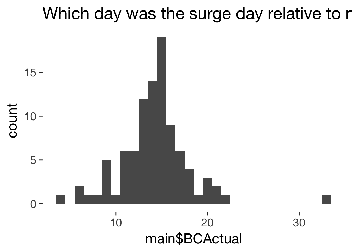
mean(main$BCActual, na.rm = T)
14.26
sd(main$BCActual, na.rm = T)
3.813
mean(main$BCActual, na.rm = T, trim = 0.1)
14.21
mad(main$BCActual, na.rm = T)
2.965
qplot(main$FCDay)
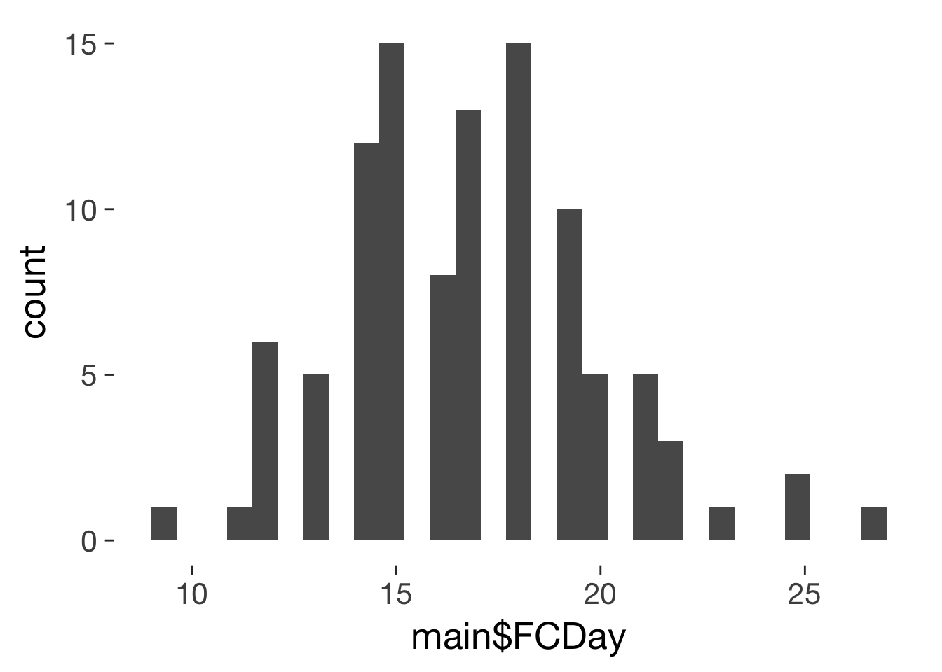
mean(main$FCDay, na.rm = T)
16.8
sd(main$FCDay, na.rm = T)
3.163
mad(main$FCDay, na.rm = T)
2.965
When does ovulation occur by cycle length?
main = main %>% filter(LengthTestingCycle<50)
xtabs(~ I(BCActual + FCDay - 1) == LengthTestingCycle, data = main)
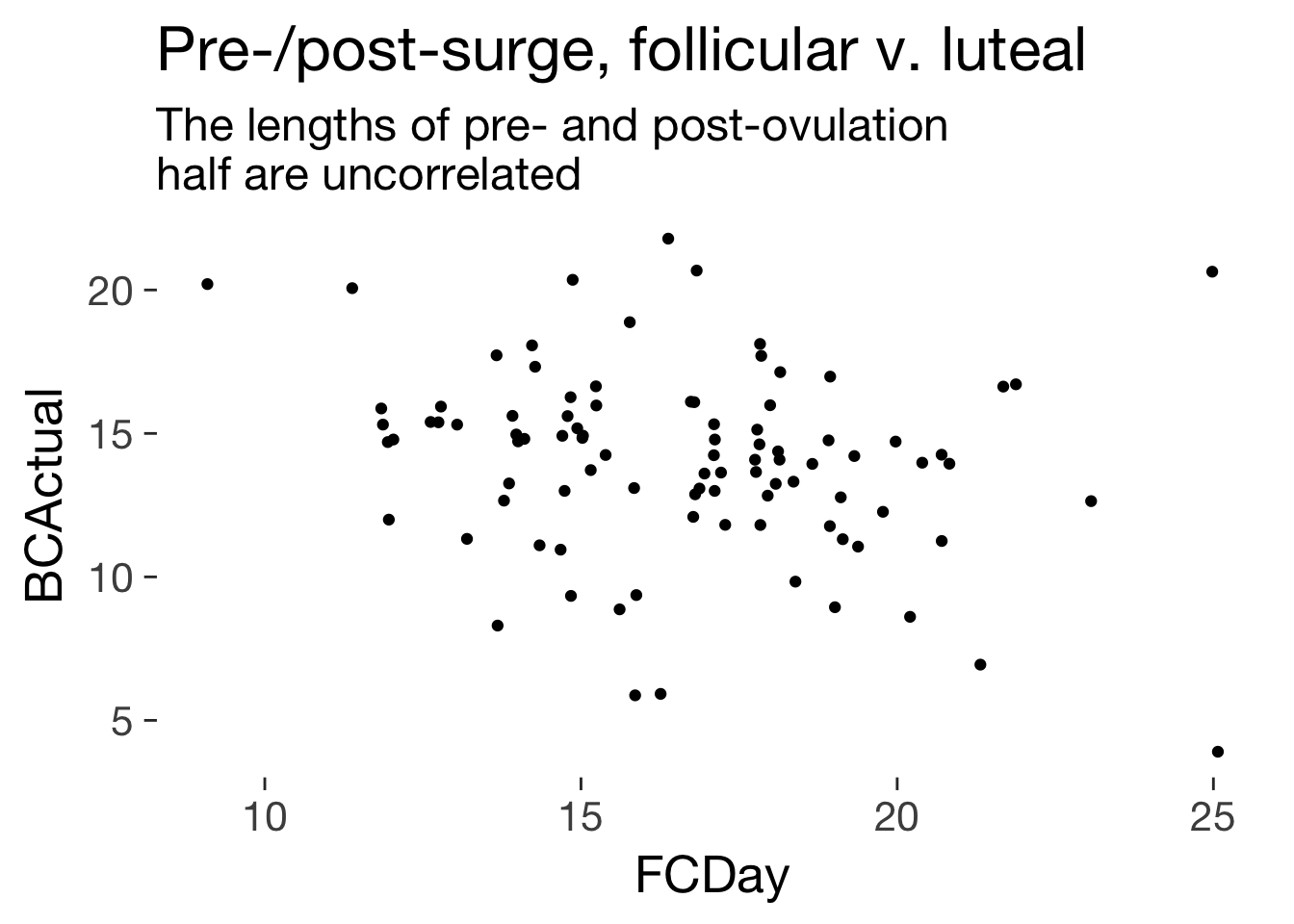
ggplot(main, aes(FCDay, BCActual)) + geom_jitter() + ggtitle("Pre-/post-surge, follicular v. luteal", subtitle = "The lengths of pre- and post-ovulation \nhalf are uncorrelated")
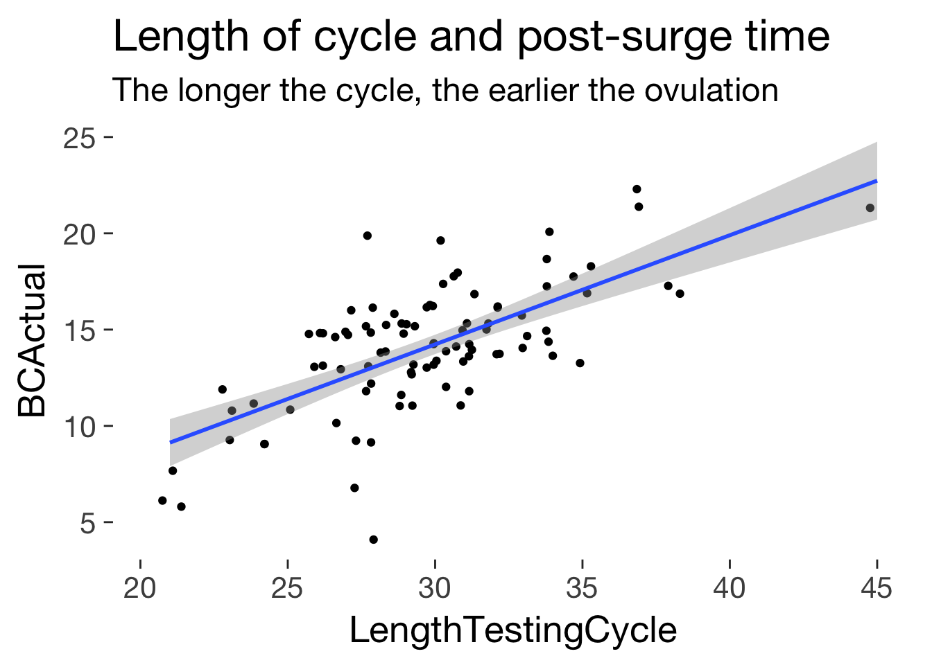
ggplot(main, aes(LengthTestingCycle, BCActual)) + geom_jitter()+ ggtitle("Length of cycle and post-surge time", subtitle = "The longer the cycle, the earlier the ovulation") + geom_smooth(method = 'lm')
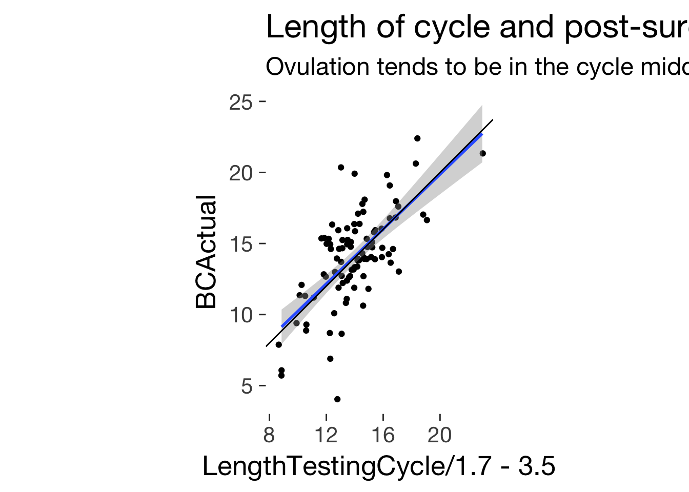
ggplot(main, aes(LengthTestingCycle/1.7 - 3.5, BCActual)) + geom_jitter()+ ggtitle("Length of cycle and post-surge time", subtitle = "Ovulation tends to be in the cycle middle") + geom_smooth(method = 'lm') + geom_abline(slope = 1) + coord_fixed()
lm(BCActual ~ LengthTestingCycle, data = main)
Fitting linear model: BCActual ~ LengthTestingCycle
| LengthTestingCycle |
0.5668 |
0.06455 |
8.781 |
8.356e-14 |
| (Intercept) |
-2.772 |
1.934 |
-1.434 |
0.155 |
cor.test(main$LengthTestingCycle, main$BCActual)
Pearson’s product-moment correlation: main$LengthTestingCycle and main$BCActual
| 8.781 |
92 |
8.356e-14 * * * |
two.sided |
cor.test(main$LengthTestingCycle, main$FCDay)
Pearson’s product-moment correlation: main$LengthTestingCycle and main$FCDay
| 6.711 |
92 |
0.000000001556 * * * |
two.sided |
lm(BCActual ~ I(LengthTestingCycle/2), data = main)
Fitting linear model: BCActual ~ I(LengthTestingCycle/2)
| I(LengthTestingCycle/2) |
1.134 |
0.1291 |
8.781 |
8.356e-14 |
| (Intercept) |
-2.772 |
1.934 |
-1.434 |
0.155 |
lm(BCActual ~ LengthTestingCycle, data = main %>% filter(LengthTestingCycle < 40))
Fitting linear model: BCActual ~ LengthTestingCycle
| LengthTestingCycle |
0.5892 |
0.07078 |
8.324 |
8.123e-13 |
| (Intercept) |
-3.415 |
2.106 |
-1.621 |
0.1084 |
lm(BCActual ~ I(LengthTestingCycle/2), data = main %>% filter(LengthTestingCycle < 40))
Fitting linear model: BCActual ~ I(LengthTestingCycle/2)
| I(LengthTestingCycle/2) |
1.178 |
0.1416 |
8.324 |
8.123e-13 |
| (Intercept) |
-3.415 |
2.106 |
-1.621 |
0.1084 |
lm(BCActual ~ I(LengthTestingCycle/2 - 3), data = main %>% filter(LengthTestingCycle < 40))
Fitting linear model: BCActual ~ I(LengthTestingCycle/2 - 3)
| I(LengthTestingCycle/2 - 3) |
1.178 |
0.1416 |
8.324 |
8.123e-13 |
| (Intercept) |
0.1205 |
1.685 |
0.07152 |
0.9431 |
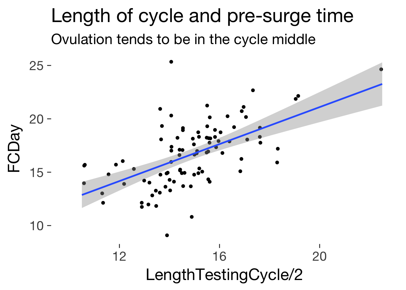
ggplot(main, aes(LengthTestingCycle/2, FCDay)) + geom_jitter()+ ggtitle("Length of cycle and pre-surge time", subtitle = "Ovulation tends to be in the cycle middle") + geom_smooth(method = 'lm')
lm(FCDay ~ I(LengthTestingCycle/2 + 5), data = main %>% filter(LengthTestingCycle < 40))
Fitting linear model: FCDay ~ I(LengthTestingCycle/2 + 5)
| I(LengthTestingCycle/2 + 5) |
0.8216 |
0.1416 |
5.804 |
0.00000009353 |
| (Intercept) |
0.3069 |
2.81 |
0.1092 |
0.9133 |
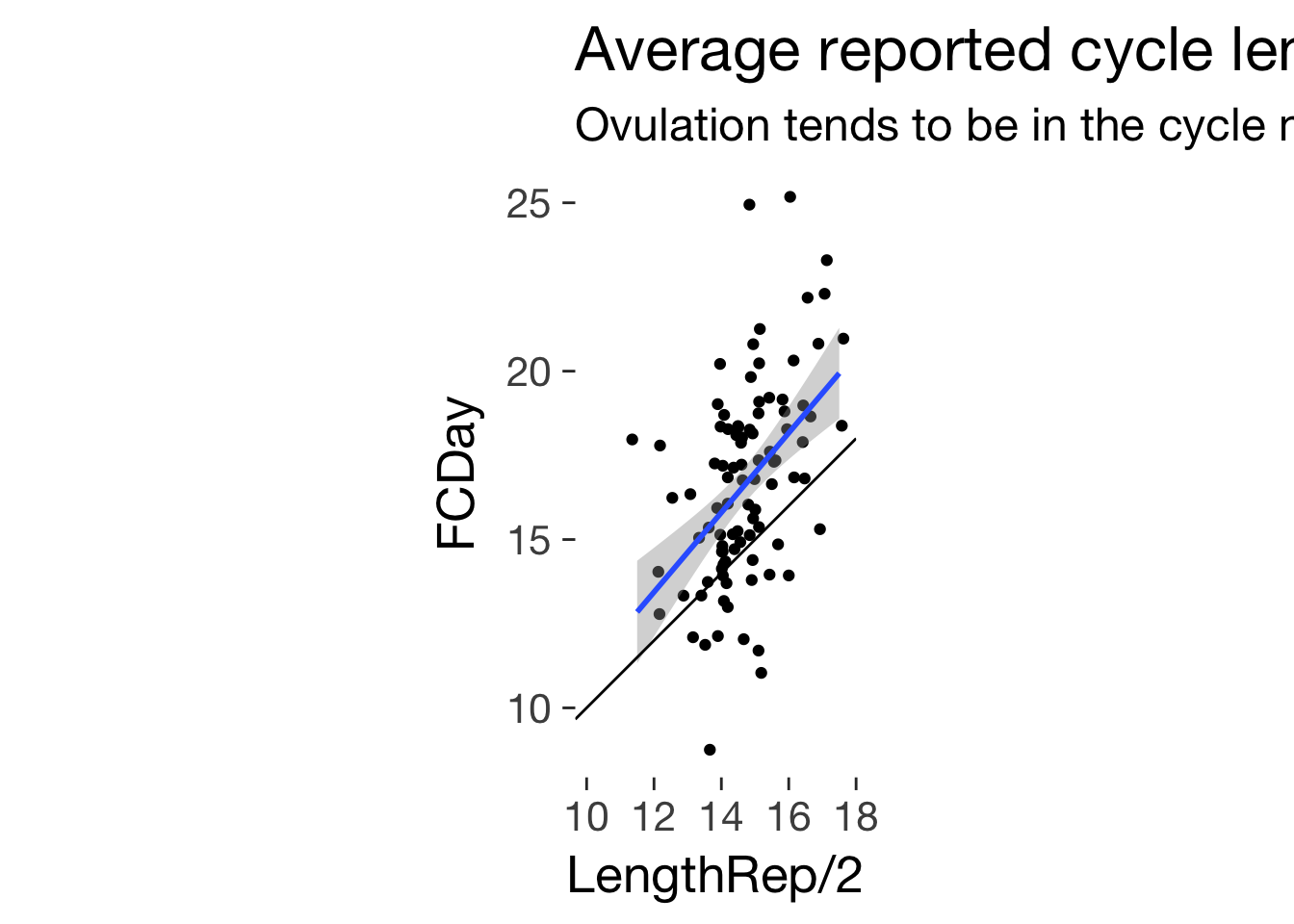
ggplot(main, aes(LengthRep/2, FCDay)) + geom_jitter()+ ggtitle("Average reported cycle length and pre-surge time", subtitle = "Ovulation tends to be in the cycle middle") + geom_smooth(method = 'lm') + geom_abline(slope = 1) + coord_fixed()
lm(FCDay ~ I(LengthRep/2), data = main %>% filter(LengthTestingCycle < 40))
Fitting linear model: FCDay ~ I(LengthRep/2)
| I(LengthRep/2) |
1.116 |
0.2175 |
5.13 |
0.000001624 |
| (Intercept) |
0.1557 |
3.206 |
0.04857 |
0.9614 |
cor.test(main$LengthRep, main$FCDay)
Pearson’s product-moment correlation: main$LengthRep and main$FCDay
| 5.285 |
92 |
0.0000008396 * * * |
two.sided |
summary(lm(BCActual ~ LengthTestingCycle + LengthRep, data = main))
| LengthTestingCycle |
0.664 |
0.07028 |
9.449 |
3.629e-15 |
| LengthRep |
-0.3349 |
0.1139 |
-2.941 |
0.004146 |
| (Intercept) |
4.192 |
3.01 |
1.393 |
0.1671 |
Fitting linear model: BCActual ~ LengthTestingCycle + LengthRep
| 94 |
2.35 |
0.5032 |
0.4923 |
Own approach
get conception risk and and arrange by FCD
To do this we subtract 9 (as the 14 days are 8 days preceding ovulation, the day of ovulation, and 5 days after) and add 14 (to obtain days relative to menstrual onset). We then add days with 0 fertility for the remaining 40-14 days of the cycle.
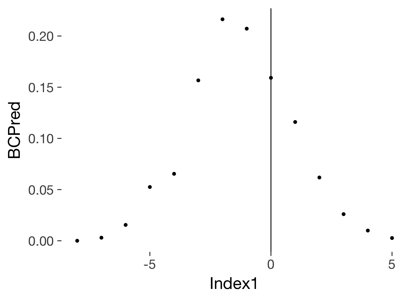
conc_risks_rel_to_ovu = conc %>%
  select(Index1, BCPred) %>% unique() %>%
  mutate(Index1 = Index1 - 9)
qplot(Index1, BCPred, data = conc_risks_rel_to_ovu) + geom_vline(xintercept = 0)
conc_risks_rel_to_ovu_interpolated = data.frame(Index1 = seq(-8, 5, 0.1)) %>%
left_join(conc_risks_rel_to_ovu)
library(mgcv)
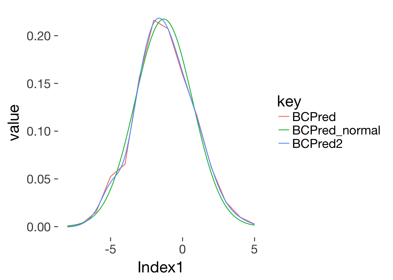
m = gam(BCPred ~ s(Index1, k = 14), data = conc_risks_rel_to_ovu)
# plot(m)
conc_risks_rel_to_ovu_interpolated$BCPred2 = as.numeric(predict(m, newdata = conc_risks_rel_to_ovu_interpolated))
cor.test(conc_risks_rel_to_ovu_interpolated$BCPred,conc_risks_rel_to_ovu_interpolated$BCPred2)
Pearson’s product-moment correlation: conc_risks_rel_to_ovu_interpolated$BCPred and conc_risks_rel_to_ovu_interpolated$BCPred2
| 84.72 |
12 |
4.882e-18 * * * |
two.sided |
normal_curve = function(x, sd, mean) {
  exp(- ( (x - mean)^2/(2 * sd^2) )) / sqrt( 2*sd^2 * pi )
}
conc_risks_rel_to_ovu_interpolated$BCPred_normal = 1.09*normal_curve(conc_risks_rel_to_ovu_interpolated$Index1, sd = 2, mean = -1.3)


conc_risks_rel_to_ovu_interpolated %>% gather(key,value,-Index1) %>%
  na.omit() %>%
ggplot(aes(Index1, value, color = key)) + geom_line()
fertile window probabilities from gangestad ea. 2006
days = data.frame(
    RCD_for_merge = c(29:1, 30:41),
    FCD = c(1:41),
    prc_stirn_b = c(.01, .01, .02, .03, .05, .09, .16, .27, .38, .48, .56, .58, .55, .48, .38, .28, .20, .14, .10, .07, .06, .04, .03, .02, .01, .01, .01, .01, .01, rep(.01, times = 12)),
#                   rep(.01, times = 70)), # gangestad uses .01 here, but I think such cases are better thrown than kept, since we might simply have missed a mens
    prc_wcx_b = c(.000, .000, .001, .002, .004, .009, .018, .032, .050, .069, .085, .094, .093, .085, .073, .059, .047, .036, .028, .021, .016, .013, .010, .008, .007, .006, .005, .005, .005, rep(.005, times = 12))
)
days$RCD = -1 * days$RCD_for_merge + 15

m = gam(prc_stirn_b ~ s(RCD, k = 14), data = days)
# plot(m)
days$prc_stirn_b2 = as.numeric(predict(m, newdata = days))
cor.test(days$prc_stirn_b,days$prc_stirn_b2)
Pearson’s product-moment correlation: days$prc_stirn_b and days$prc_stirn_b2
| 536.7 |
39 |
4.65e-77 * * * |
two.sided |
days$prc_stirn_b = days$prc_stirn_b2
expand the main dataset into long format
Essentially we’re trying to reproduce the conception risk dataset.
Best guesses as to what variables mean: - LengthTestingCycle: The length of the cycle in which women actually used the LH strips. - BCActual: The day the LH surge occurred, counted from the end of the cycle - FCDay: The day the LH surge occurred, counted from the beginning of the cycle - LengthRep: The average cycle length reported in the screening survey.
conc_risks_rel_to_ovu = conc_risks_rel_to_ovu_interpolated %>% select(Index1, BCPred2) %>% rename(BCPred = BCPred2)
long = main %>% select(Subject, Age, RelStat, LengthTestingCycle, FCDay, BCActual, LengthRep) %>%   filter(!is.na(LengthTestingCycle)) %>%  # can't use those without complete cycle
  group_by(Subject, Age, RelStat, LengthTestingCycle, FCDay, BCActual, LengthRep) %>%
  # group to retain after expanding
  expand(FCD = full_seq(1:LengthTestingCycle, period = 1)) %>%
  mutate(
         day_of_ovu_surge = FCDay + 1, # ovulation occurs one day after LH surge
         day_of_ovu_bc_est_m14 = LengthTestingCycle - 1 - 14, # counting 14 back from the next menstrual onset, minus 1 cause we're translating a length into days from 0
         day_of_ovu_fc_est_m14 = LengthRep - 1 - 14, # counting 14 back from the next menstrual onset, minus 1 cause we're translating a length into days from 0
         day_of_ovu_fc = 14,
         day_of_ovu_bc_est_half = (LengthTestingCycle - 1)/2 + 3, # three days after the middle of the cycle
         day_of_ovu_rep_half = (LengthRep - 1)/2 + 3, # three days after the middle of the cycle

         FCD0 = FCD - 1, # if we want to subtract the day of ovu, need to start counting from 0
         days_until_ovu_bc_half = FCD0 - day_of_ovu_bc_est_half ,
         days_until_ovu_rep_half = FCD0 - day_of_ovu_rep_half,
         days_until_ovu_bc_m14 = FCD0 - day_of_ovu_bc_est_m14,
         days_until_ovu_fc_m14 = FCD0 - day_of_ovu_fc_est_m14,
         days_until_ovu_fc = FCD0 - day_of_ovu_fc,
         days_until_ovu_surge = FCD0 - day_of_ovu_surge,
         days_until_ovu_bc_m14_squished = if_else(
          LengthTestingCycle - FCD < 14,
          29 - (LengthTestingCycle - FCD),
          round((FCD/ (LengthTestingCycle - 14) ) * 15)) - 15
         ) %>%
  left_join(conc_risks_rel_to_ovu %>% rename(conc_bc_m14 = BCPred), by = c("days_until_ovu_bc_m14" = "Index1")) %>%
  left_join(conc_risks_rel_to_ovu %>% rename(conc_bc_m14_sq = BCPred), by = c("days_until_ovu_bc_m14_squished" = "Index1")) %>%
  left_join(days %>% select(RCD, prc_stirn_b) %>% rename(fert_bc_m14_sq = prc_stirn_b), by = c("days_until_ovu_bc_m14_squished" = "RCD")) %>%
  left_join(days %>% select(RCD, prc_stirn_b) %>% rename(fert_bc_m14 = prc_stirn_b), by = c("days_until_ovu_bc_m14" = "RCD")) %>%
  left_join(conc_risks_rel_to_ovu %>% rename(conc_fc_m14 = BCPred), by = c("days_until_ovu_fc_m14" = "Index1")) %>%
  left_join(days %>% select(RCD, prc_stirn_b) %>% rename(fert_fc_m14 = prc_stirn_b), by = c("days_until_ovu_fc_m14" = "RCD")) %>%
  left_join(conc_risks_rel_to_ovu %>% rename(conc_ovu_fc = BCPred), by = c("days_until_ovu_fc" = "Index1")) %>%
  left_join(conc_risks_rel_to_ovu %>% rename(conc_ovu_surge = BCPred), by = c("days_until_ovu_surge" = "Index1")) %>%
  left_join(days %>% select(RCD, prc_stirn_b) %>% rename(fert_ovu_surge = prc_stirn_b), by = c("days_until_ovu_surge" = "RCD")) %>%
  mutate(
         conc_bc_m14 = if_else(is.na(conc_bc_m14), 0, conc_bc_m14),
         conc_fc_m14 = if_else(is.na(conc_fc_m14), 0, conc_fc_m14),
         conc_ovu_fc = if_else(is.na(conc_ovu_fc), 0, conc_ovu_fc),
         conc_ovu_surge = if_else(is.na(conc_ovu_surge), 0, conc_ovu_surge)
         ) %>%
  ungroup()

# View(long %>% select(Subject, FCD, RCD, ovu_day_fcd, ovu_day_rcd) %>% filter(ovu_day_rcd|ovu_day_fcd))
# ggplot(long %>% filter(Subject==2), aes(days_until_ovu_rep_half, conc_rep_half))+geom_point() + geom_vline(xintercept=0)
# ggplot(long %>% filter(Subject==2), aes(days_until_ovu_bc_m14, conc_bc_m14))+geom_point() + geom_vline(xintercept=0)
# ggplot(long %>% filter(Subject==2), aes(days_until_ovu_fc, conc_ovu_fc))+geom_point() + geom_vline(xintercept=0)
# ggplot(long %>% filter(Subject==2), aes(days_until_ovu_surge, conc_ovu_surge))+geom_point() + geom_vline(xintercept=0)

# ggplot(long %>% filter(Subject==2), aes(days_until_ovu_bc_half, days_until_ovu_surge))+geom_point() + geom_abline(slope = 1)
# ggplot(long %>% filter(Subject==2), aes(days_until_ovu_bc_m14, days_until_ovu_surge))+geom_point() + geom_abline(slope = 1)
conception risk correlations
long %>% select(starts_with("conc_")) %>% cor(use='pairwise.complete.obs') %>% round(2)# %>% .[,5]
| conc_bc_m14 |
1 |
0.94 |
0.54 |
0.49 |
0.36 |
| conc_bc_m14_sq |
0.94 |
1 |
0.4 |
0.36 |
0.24 |
| conc_fc_m14 |
0.54 |
0.4 |
1 |
0.66 |
0.34 |
| conc_ovu_fc |
0.49 |
0.36 |
0.66 |
1 |
0.29 |
| conc_ovu_surge |
0.36 |
0.24 |
0.34 |
0.29 |
1 |
fertile window probability correlations
The day of the next menstrual onset minus 14 (with “squishing” of fertile phase probabilities in the follicular phase) is the index we used in our manuscript fert_bc_m14_sq. fert_ovu_surge is the probability of being in the fertile window when using the day of ovulation estimated using the LH surge.
print(cor.test(long$fert_bc_m14_sq, long$fert_ovu_surge)) # does not properly treat the nested structure of the data
##
##  Pearson's product-moment correlation
##
## data:  long$fert_bc_m14_sq and long$fert_ovu_surge
## t = 37, df = 2800, p-value <2e-16
## alternative hypothesis: true correlation is not equal to 0
## 95 percent confidence interval:
##  0.5456 0.5959
## sample estimates:
##    cor
## 0.5713
long %>% group_by(Subject) %>%
  filter(!is.na(fert_bc_m14_sq), !is.na(fert_ovu_surge)) %>%
  summarise(corr = cor(fert_bc_m14_sq, fert_ovu_surge, use = 'pairwise.complete.obs')) %>%
  ungroup() %>%
  summarise(cor = mean(corr), cor_sd = sd(corr), n = n()) %>% # to get a sense of interindividual variation in the corr
  pander::pander()
long %>% select(starts_with("fert_")) %>% cor(use='pairwise.complete.obs') %>% round(2)# %>% .[,5]
| fert_bc_m14_sq |
1 |
0.94 |
0.72 |
0.57 |
| fert_bc_m14 |
0.94 |
1 |
0.66 |
0.56 |
| fert_fc_m14 |
0.72 |
0.66 |
1 |
0.53 |
| fert_ovu_surge |
0.57 |
0.56 |
0.53 |
1 |
subset to cycles 25-33
long %>% filter(LengthTestingCycle %in% 25:33) %>% select(starts_with("conc_")) %>% cor(use='na.or.complete') %>% round(2)
| conc_bc_m14 |
1 |
0.98 |
0.55 |
0.59 |
0.22 |
| conc_bc_m14_sq |
0.98 |
1 |
0.56 |
0.65 |
0.22 |
| conc_fc_m14 |
0.55 |
0.56 |
1 |
0.56 |
0.2 |
| conc_ovu_fc |
0.59 |
0.65 |
0.56 |
1 |
0.1 |
| conc_ovu_surge |
0.22 |
0.22 |
0.2 |
0.1 |
1 |
mean fertility on day of ovulation
long %>% filter(days_until_ovu_surge %in% -2:0) %>%
  ungroup() %>%
  select(starts_with("conc")) %>%
  summarise_each(funs(mean)) %>% pander()
| 0.07985 |
NA |
0.07522 |
0.07029 |
0.194 |
days until ovulation
long %>% select(starts_with("days_until_ovu")) %>% cor(use='na.or.complete') %>% round(2)
| days_until_ovu_bc_half |
1 |
0.98 |
0.98 |
0.97 |
0.98 |
0.96 |
0.98 |
| days_until_ovu_rep_half |
0.98 |
1 |
0.92 |
0.99 |
0.99 |
0.96 |
0.95 |
| days_until_ovu_bc_m14 |
0.98 |
0.92 |
1 |
0.92 |
0.9 |
0.94 |
0.98 |
| days_until_ovu_fc_m14 |
0.97 |
0.99 |
0.92 |
1 |
0.96 |
0.95 |
0.94 |
| days_until_ovu_fc |
0.98 |
0.99 |
0.9 |
0.96 |
1 |
0.95 |
0.93 |
| days_until_ovu_surge |
0.96 |
0.96 |
0.94 |
0.95 |
0.95 |
1 |
0.94 |
| days_until_ovu_bc_m14_squished |
0.98 |
0.95 |
0.98 |
0.94 |
0.93 |
0.94 |
1 |
long %>% filter(!duplicated(Subject)) %>% select(starts_with("day_of_ovu"))  %>% ungroup() %>%
  gather(key, value, -day_of_ovu_surge) %>%
  group_by(key) %>%
  do(cbind(mean_v =mean(.$value), describe(.$value - .$day_of_ovu_surge))) %>%
  select(key, mean_v, mean, sd, median, min, max) %>%
  rename(mean_diff = mean, mean = mean_v) %>%
  pander()
| day_of_ovu_bc_est_half |
17.24 |
-0.2872 |
2.447 |
-0.5 |
-9.5 |
6.5 |
| day_of_ovu_bc_est_m14 |
14.49 |
-2.936 |
3.298 |
-3 |
-13 |
5 |
| day_of_ovu_fc |
14 |
-3.638 |
2.969 |
-4 |
-12 |
4 |
| day_of_ovu_fc_est_m14 |
14.14 |
-3.223 |
2.783 |
-3 |
-11 |
3 |
| day_of_ovu_rep_half |
17.07 |
-0.4309 |
2.61 |
-0.5 |
-8.5 |
6 |
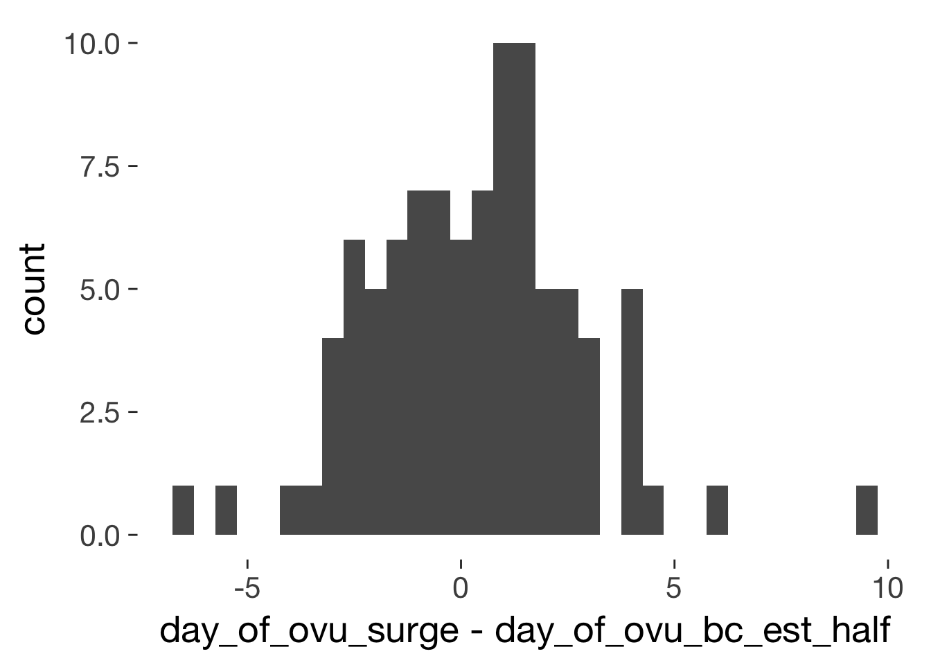
xsect = long %>% filter(!duplicated(Subject)) %>% ungroup()
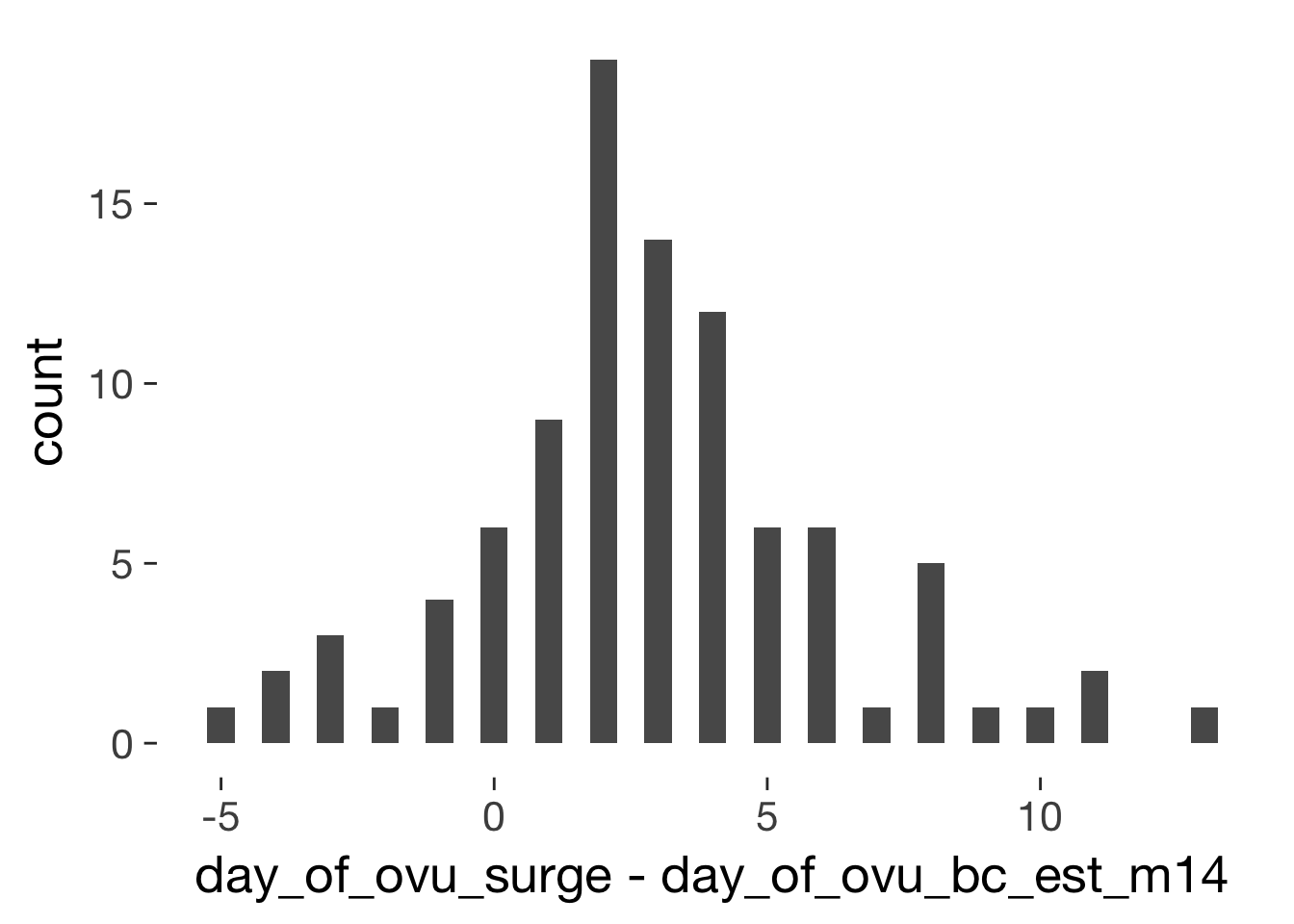
qplot(day_of_ovu_surge - day_of_ovu_bc_est_m14, data=xsect, binwidth = 0.5)
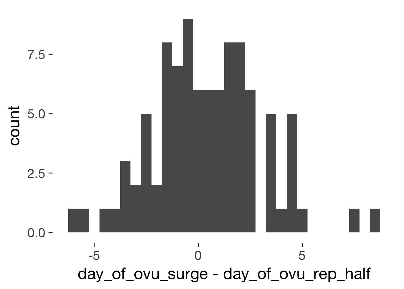
qplot(day_of_ovu_surge - day_of_ovu_rep_half, data=xsect, binwidth = 0.5)
qplot(day_of_ovu_surge - day_of_ovu_bc_est_half, data=xsect, binwidth = 0.5)