Item-level model for extra-pair items
Cycling women (not on hormonal birth control)
Women on hormonal birth control
Load data
library(knitr)
opts_chunk$set(fig.width = 12, fig.height = 12, cache = F, warning = F, message = F)
library(formr); library(data.table); library(stringr); library(ggplot2); library(plyr); library(dplyr);library(car); library(psych);
source("0_helpers.R")
library(brms)
load("full_data.rdata")
diary$included = diary$included_all
diary_long = diary %>% group_by(person) %>%
filter(!is.na(included_all), !is.na(fertile_fab)) %>%
mutate(included = included_all,
fertile = fertile_fab,
fertile_mean = mean(fertile_fab, na.rm = T)) %>%
select(person, menstruation, RCD_inferred, fertile_mean, fertile, fertile_fab, included, extra_pair_2, extra_pair_3, extra_pair_4, extra_pair_5, extra_pair_6, extra_pair_7, extra_pair_8, extra_pair_9, extra_pair_10, extra_pair_11, extra_pair_12, extra_pair_13) %>%
tidyr::gather(variable, value, -person, -menstruation, -fertile_mean,-fertile, -fertile_fab, -included, -RCD_inferred)
items = xlsx::read.xlsx("item_tables/Daily_items_bearbeitetAM.xlsx", 1)
diary_long = diary_long %>% left_join(items %>% select(Item.name, Item), by = c("variable" = "Item.name"))Splines BC, adjusted
Splines over backward-counted cycle days, adjusting for menstruation and average fertility, allowing the menstruation and hormonal contraception dummy effects to vary by item.
Model summary
long_rcd = readRDS("3_brms_extra_pair_long_rcd.rds")
summary(long_rcd)
## Family: cumulative(logit)
## Formula: value ~ included * menstruation + s(RCD_inferred, by = included) + fertile_mean + (1 | person) + (1 + included * menstruation | variable)
## disc = 1
## Data: diary_long (Number of observations: 169380)
## Samples: 9 chains, each with iter = 2000; warmup = 1000; thin = 1;
## total post-warmup samples = 9000
## ICs: LOO = 285281.18; WAIC = 285279.91
##
## Smooth Terms:
## Estimate Est.Error l-95% CI u-95% CI Eff.Sample Rhat
## sds(sRCD_inferredincludedcycling_1) 0.82 0.39 0.34 1.85 2758 1
## sds(sRCD_inferredincludedhorm_contra_1) 1.45 0.74 0.48 3.33 1916 1
##
## Group-Level Effects:
## ~person (Number of levels: 723)
## Estimate Est.Error l-95% CI u-95% CI Eff.Sample Rhat
## sd(Intercept) 1.28 0.04 1.21 1.36 379 1.03
##
## ~variable (Number of levels: 12)
## Estimate Est.Error l-95% CI
## sd(Intercept) 1.06 0.27 0.68
## sd(includedhorm_contra) 0.39 0.09 0.26
## sd(menstruationpre) 0.10 0.04 0.04
## sd(menstruationyes) 0.06 0.04 0.00
## sd(includedhorm_contra:menstruationpre) 0.06 0.04 0.00
## sd(includedhorm_contra:menstruationyes) 0.05 0.04 0.00
## cor(Intercept,includedhorm_contra) 0.14 0.24 -0.34
## cor(Intercept,menstruationpre) 0.17 0.27 -0.37
## cor(includedhorm_contra,menstruationpre) 0.41 0.26 -0.16
## cor(Intercept,menstruationyes) -0.14 0.33 -0.72
## cor(includedhorm_contra,menstruationyes) 0.33 0.32 -0.40
## cor(menstruationpre,menstruationyes) 0.11 0.34 -0.58
## cor(Intercept,includedhorm_contra:menstruationpre) -0.07 0.34 -0.70
## cor(includedhorm_contra,includedhorm_contra:menstruationpre) -0.38 0.34 -0.88
## cor(menstruationpre,includedhorm_contra:menstruationpre) -0.26 0.35 -0.83
## cor(menstruationyes,includedhorm_contra:menstruationpre) -0.19 0.36 -0.80
## cor(Intercept,includedhorm_contra:menstruationyes) 0.00 0.36 -0.67
## cor(includedhorm_contra,includedhorm_contra:menstruationyes) 0.20 0.37 -0.56
## cor(menstruationpre,includedhorm_contra:menstruationyes) 0.02 0.37 -0.68
## cor(menstruationyes,includedhorm_contra:menstruationyes) 0.02 0.38 -0.69
## cor(includedhorm_contra:menstruationpre,includedhorm_contra:menstruationyes) -0.08 0.37 -0.74
## u-95% CI Eff.Sample Rhat
## sd(Intercept) 1.70 1719 1.00
## sd(includedhorm_contra) 0.60 2374 1.00
## sd(menstruationpre) 0.19 2718 1.00
## sd(menstruationyes) 0.14 3226 1.00
## sd(includedhorm_contra:menstruationpre) 0.14 3323 1.00
## sd(includedhorm_contra:menstruationyes) 0.15 3908 1.00
## cor(Intercept,includedhorm_contra) 0.59 2010 1.01
## cor(Intercept,menstruationpre) 0.66 4942 1.00
## cor(includedhorm_contra,menstruationpre) 0.83 3670 1.00
## cor(Intercept,menstruationyes) 0.53 7701 1.00
## cor(includedhorm_contra,menstruationyes) 0.83 6156 1.00
## cor(menstruationpre,menstruationyes) 0.72 6871 1.00
## cor(Intercept,includedhorm_contra:menstruationpre) 0.60 9000 1.00
## cor(includedhorm_contra,includedhorm_contra:menstruationpre) 0.41 4495 1.00
## cor(menstruationpre,includedhorm_contra:menstruationpre) 0.49 5841 1.00
## cor(menstruationyes,includedhorm_contra:menstruationpre) 0.56 4930 1.00
## cor(Intercept,includedhorm_contra:menstruationyes) 0.68 9000 1.00
## cor(includedhorm_contra,includedhorm_contra:menstruationyes) 0.79 6421 1.00
## cor(menstruationpre,includedhorm_contra:menstruationyes) 0.71 9000 1.00
## cor(menstruationyes,includedhorm_contra:menstruationyes) 0.72 6973 1.00
## cor(includedhorm_contra:menstruationpre,includedhorm_contra:menstruationyes) 0.64 6408 1.00
##
## Population-Level Effects:
## Estimate Est.Error l-95% CI u-95% CI Eff.Sample Rhat
## Intercept[1] 1.33 0.34 0.66 2.00 865 1.01
## Intercept[2] 1.79 0.34 1.13 2.47 865 1.01
## Intercept[3] 2.27 0.34 1.60 2.95 865 1.01
## Intercept[4] 3.18 0.34 2.51 3.86 864 1.01
## Intercept[5] 4.03 0.34 3.35 4.71 864 1.01
## includedhorm_contra -0.20 0.16 -0.50 0.12 258 1.04
## menstruationpre -0.07 0.06 -0.18 0.05 3409 1.00
## menstruationyes -0.15 0.04 -0.24 -0.07 4173 1.00
## fertile_mean -0.21 0.75 -1.75 1.24 389 1.04
## includedhorm_contra:menstruationpre 0.09 0.07 -0.05 0.23 4126 1.00
## includedhorm_contra:menstruationyes 0.09 0.06 -0.03 0.21 5662 1.00
## sRCD_inferred:includedcycling_1 -0.04 0.17 -0.36 0.30 3264 1.00
## sRCD_inferred:includedhorm_contra_1 0.16 0.30 -0.31 0.88 2096 1.00
##
## Samples were drawn using sampling(NUTS). For each parameter, Eff.Sample
## is a crude measure of effective sample size, and Rhat is the potential
## scale reduction factor on split chains (at convergence, Rhat = 1).Marginal effect plots
# by_item = items %>% select(Item.name, Item) %>% unique()
# rownames(by_item) = by_item$Item
# marge = plot(marginal_effects(long_rcd, re_formula = ~ (1 + included * menstruation | variable), conditions = by_item), plot = F)
# marge$`RCD_inferred:included` = marge$`RCD_inferred:included` + scale_x_reverse(limits = c(30,0)) + facet_wrap(~ cond__, scales = "free_y")
# marge

smo = marginal_smooths(long_rcd)
smo2 = smo$`mu: s(RCD_inferred,by=included)` %>% mutate(included = as.character(included)) %>% bind_rows(
  diary %>% mutate(
    RCD_inferred = -1*RCD, included = 'conc',estimate__ = prc_stirn_b/1.2 - 0.25) %>%
    select(included, RCD_inferred, estimate__) %>%
    filter(RCD_inferred < 30 ) %>% unique())
ggplot(smo2, aes(RCD_inferred, estimate__, color = included, fill = included, linetype = included)) +
  geom_ribbon(aes(ymin = lower__, ymax = upper__), alpha = 0.2, color = NA) +
  geom_line(size = 0.8, stat = "identity") +
  scale_color_manual("", values = c("horm_contra" = "black", "cycling" = "red", "conc" = "#a83fbf"), labels = c("horm_contra"="hormonal contraception user","1"="naturally cycling", "conc" = "superimposed conception risk"))+
  scale_fill_manual("", values = c("horm_contra" = "black", "cycling" = "red", "conc" = "#a83fbf"), labels = c("horm_contra"="hormonal contraception user","1"="naturally cycling", "conc" = "superimposed conception risk")) +
  scale_linetype_manual(values = c("horm_contra" = "solid", "cycling" = "solid", "conc" = "dashed"), guide = F) +
  scale_x_reverse() +
  coord_cartesian(xlim = c(0,30), ylim = c(-0.25, 0.25))
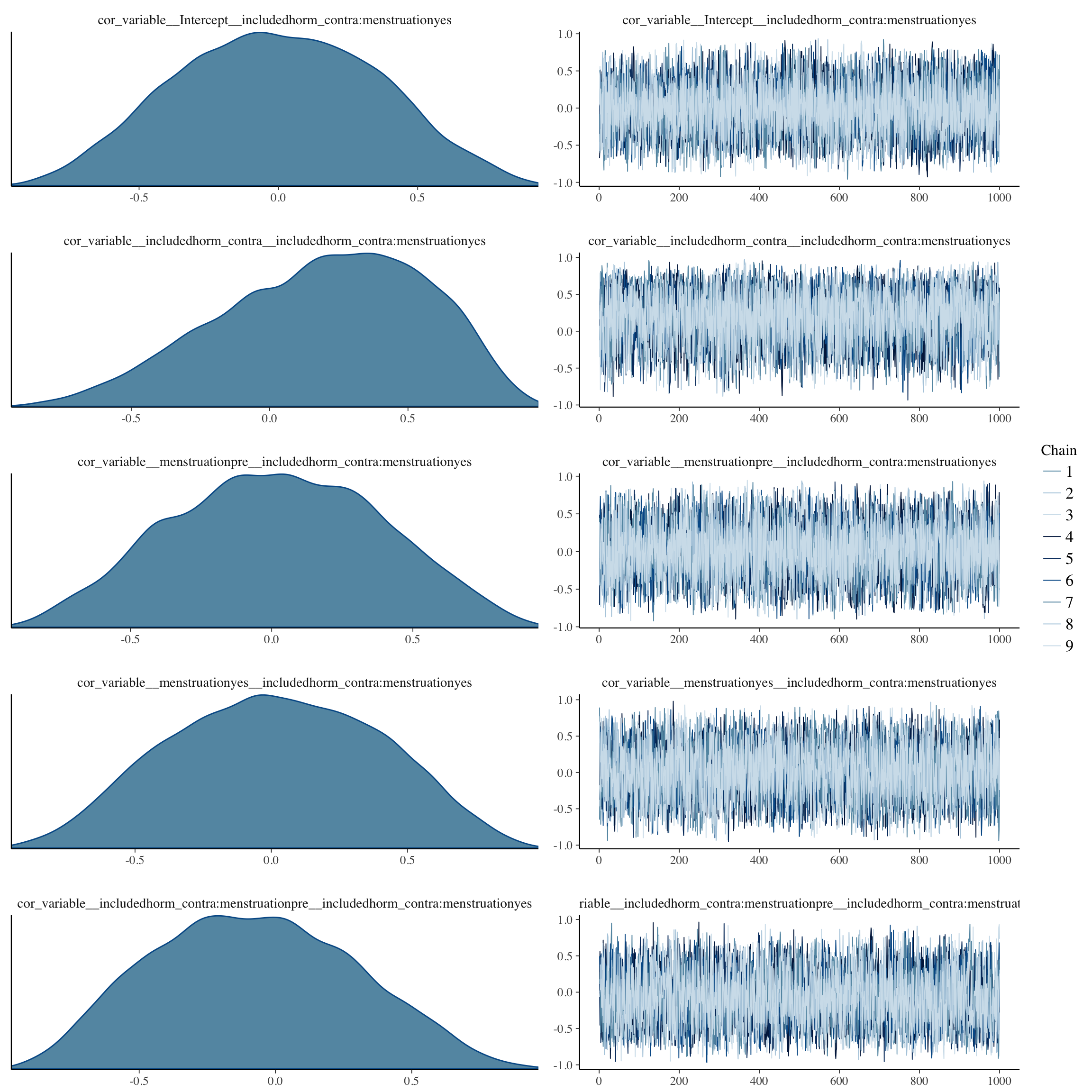
Coefficient plots
bayesplot::mcmc_areas(as.matrix(long_rcd$fit), regex_pars = "b_[^I]")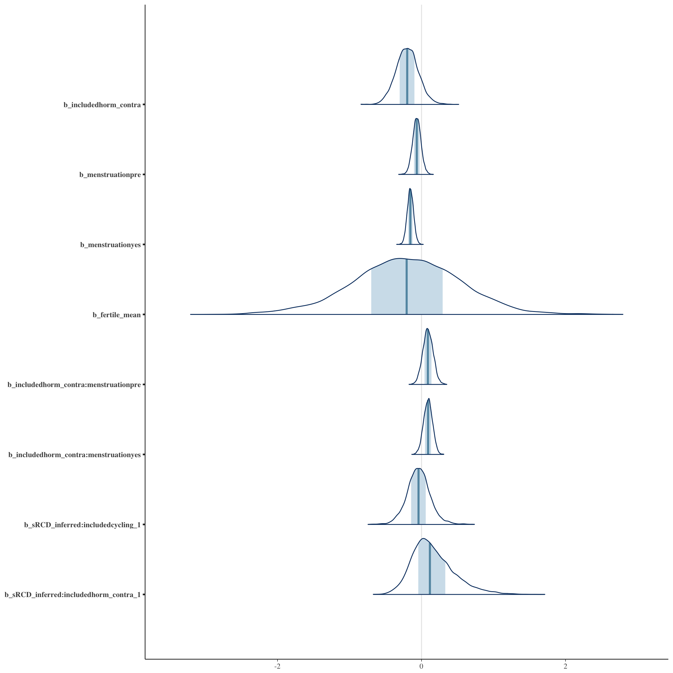
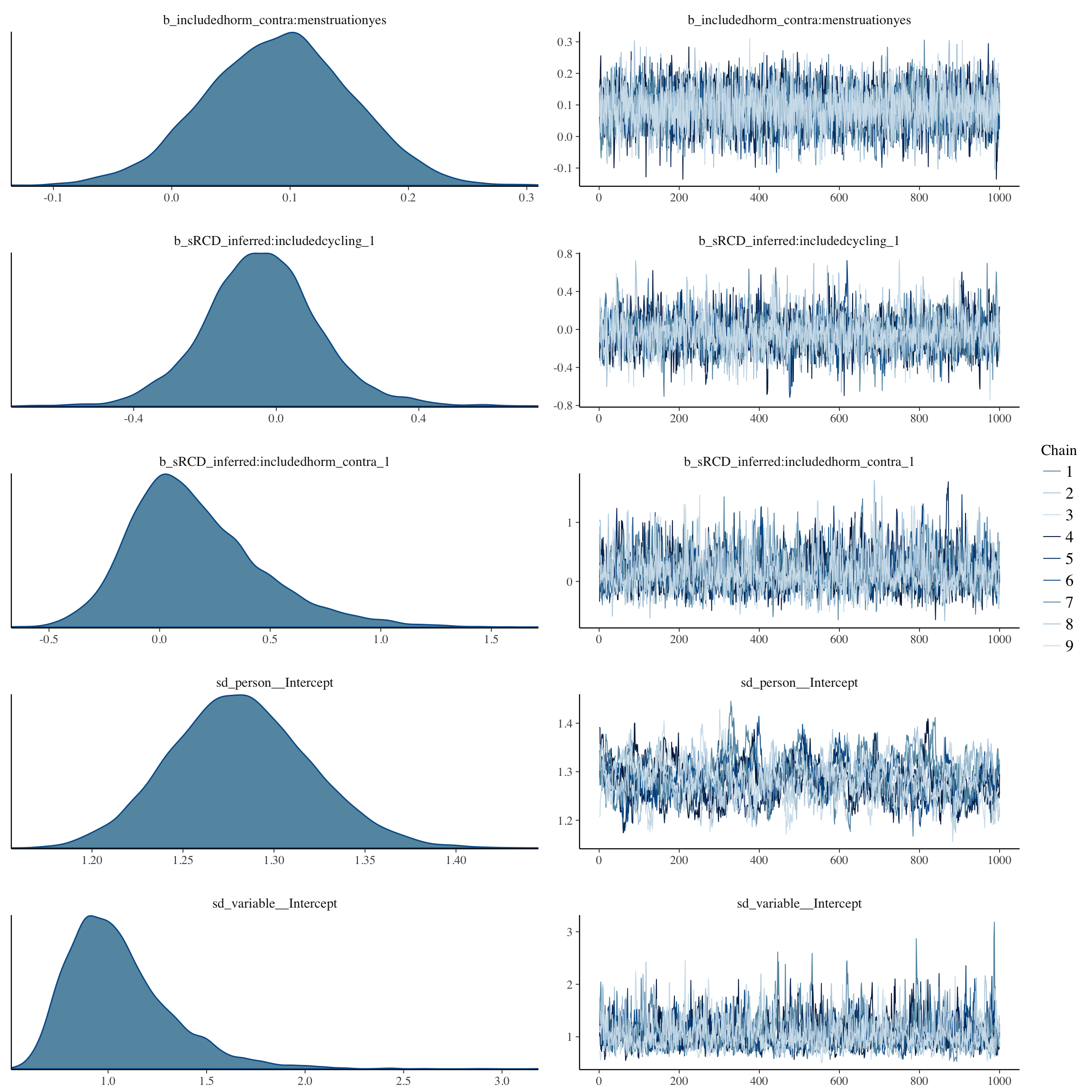
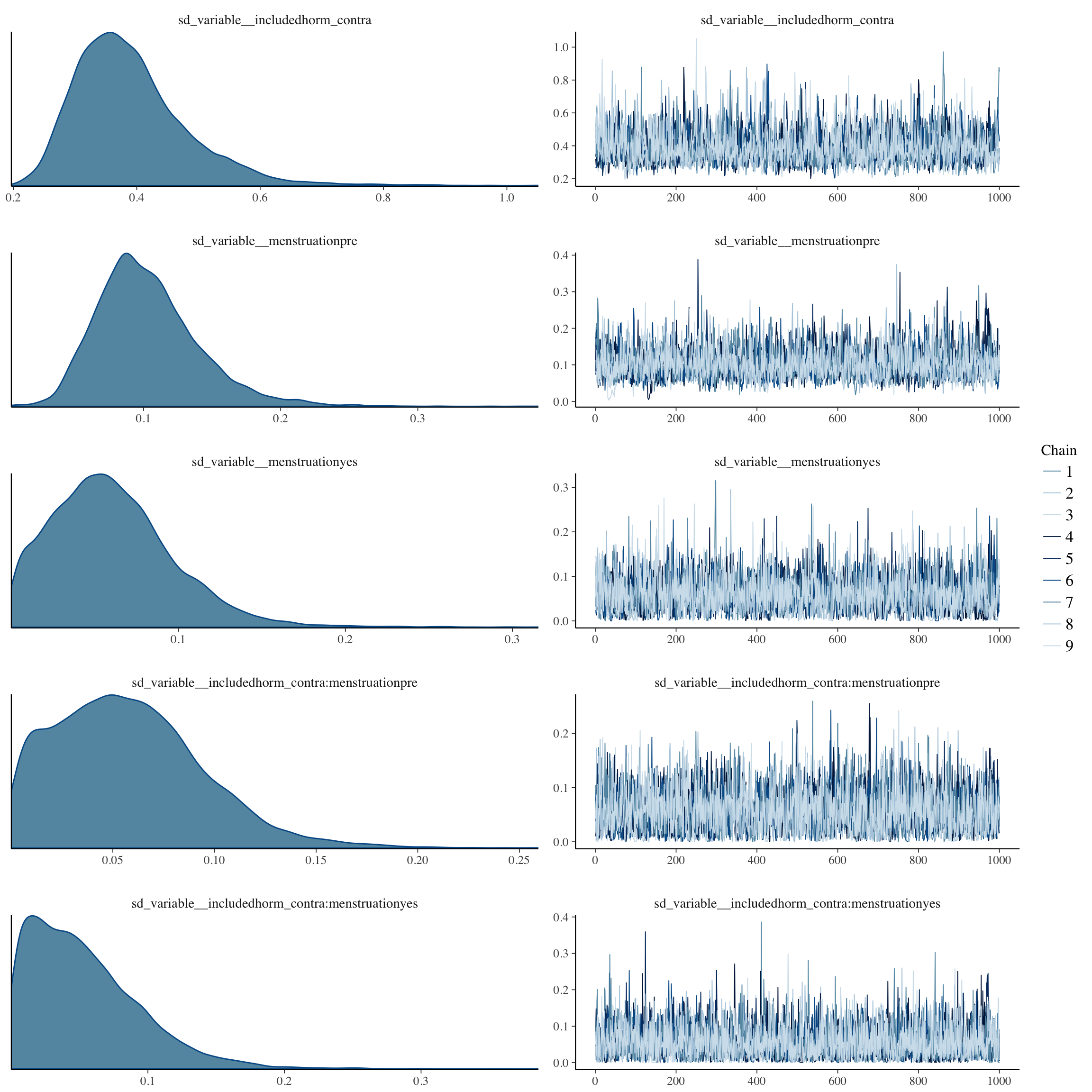
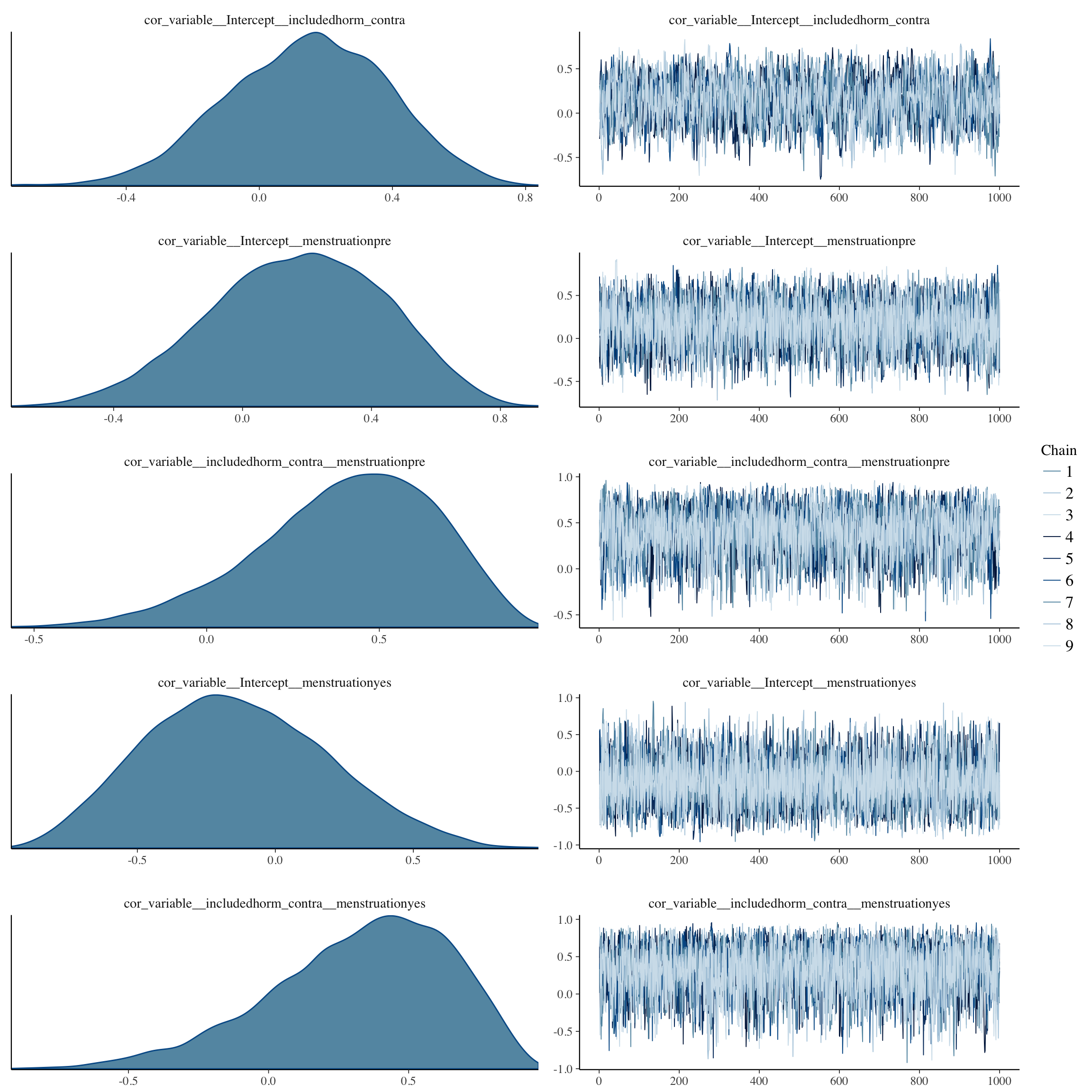
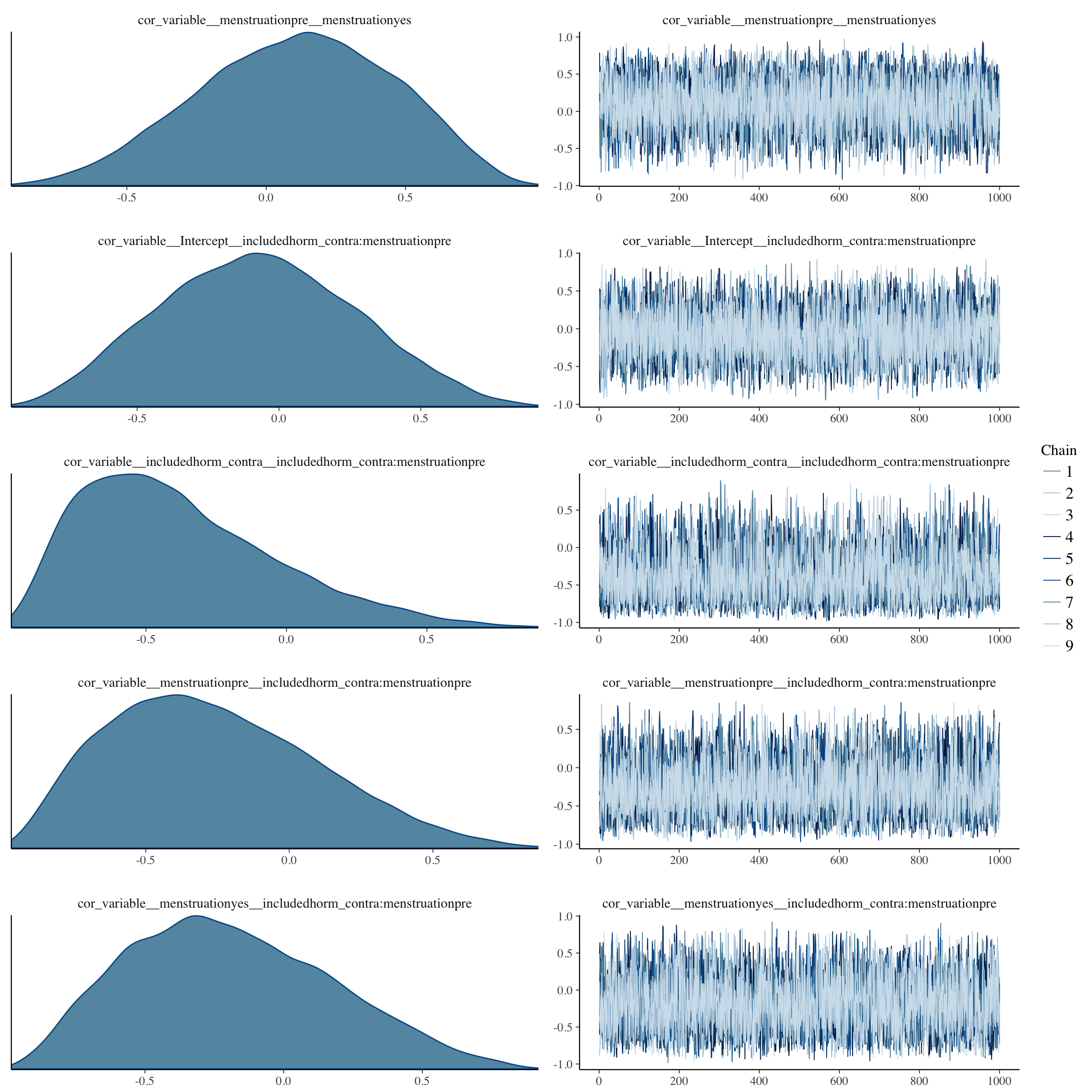
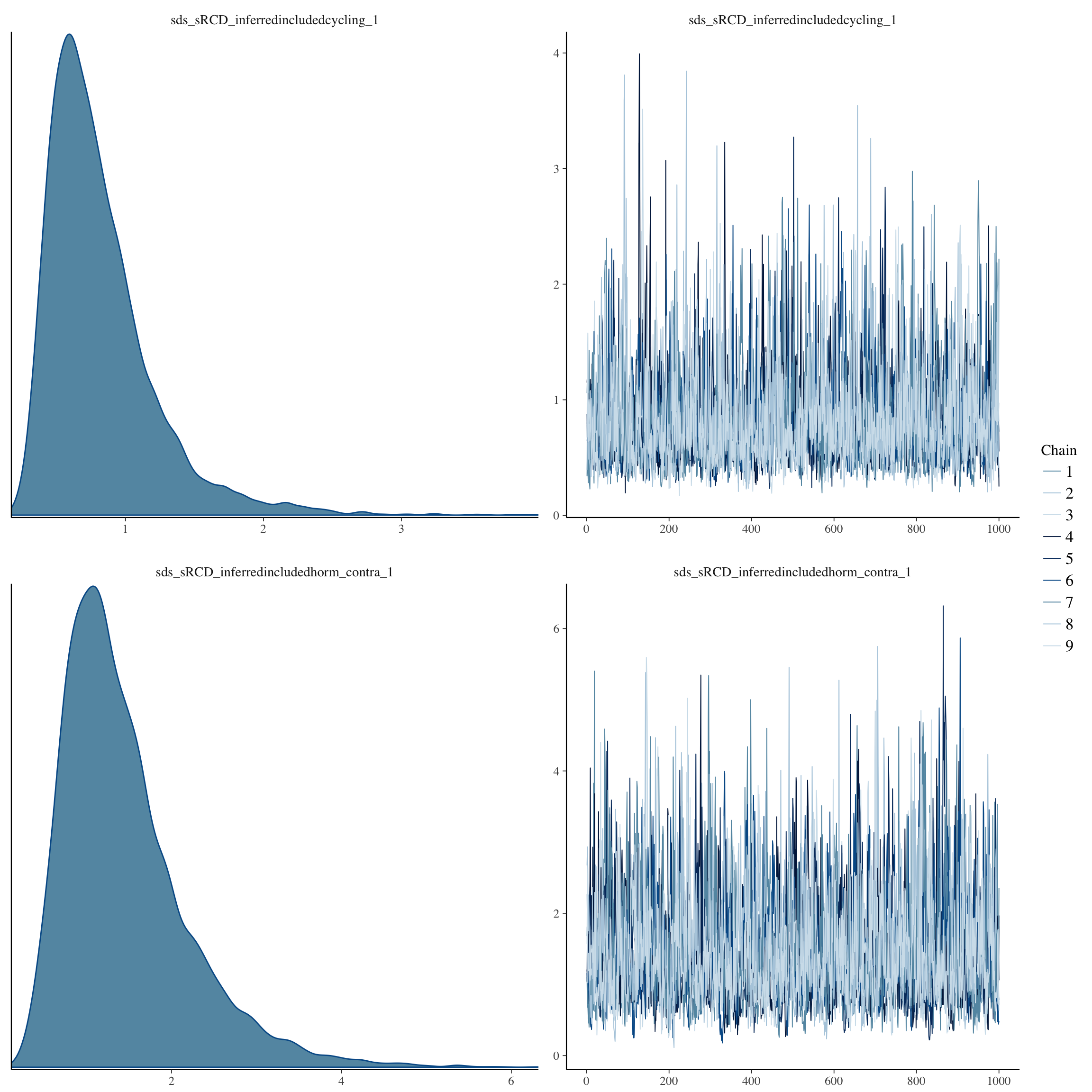
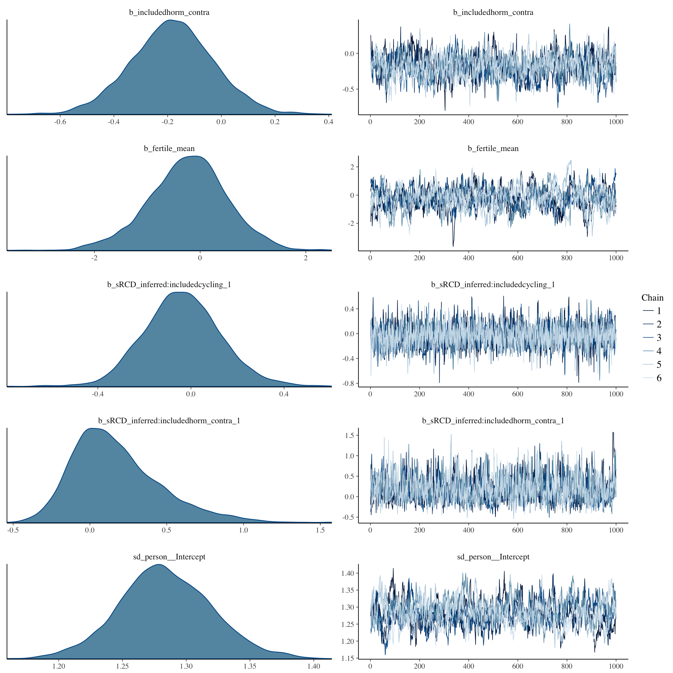
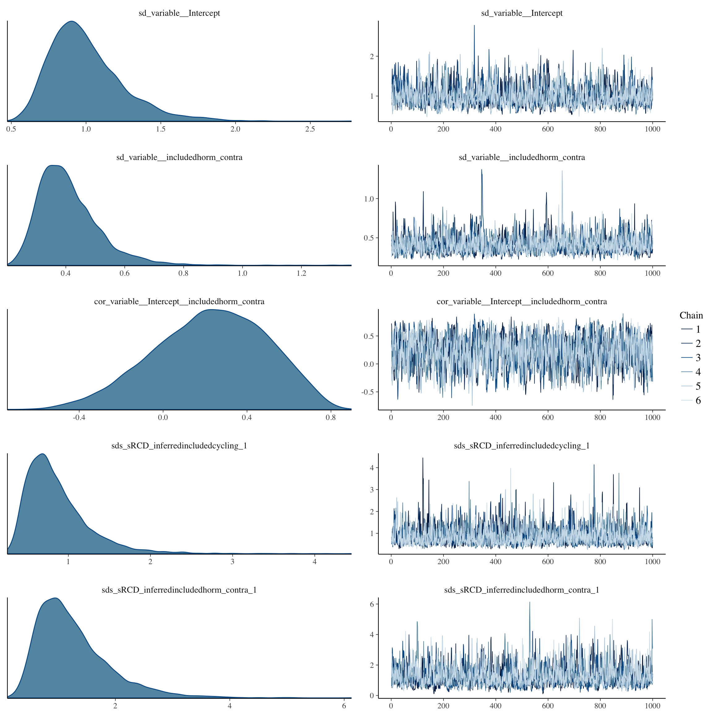
Diagnostic plots
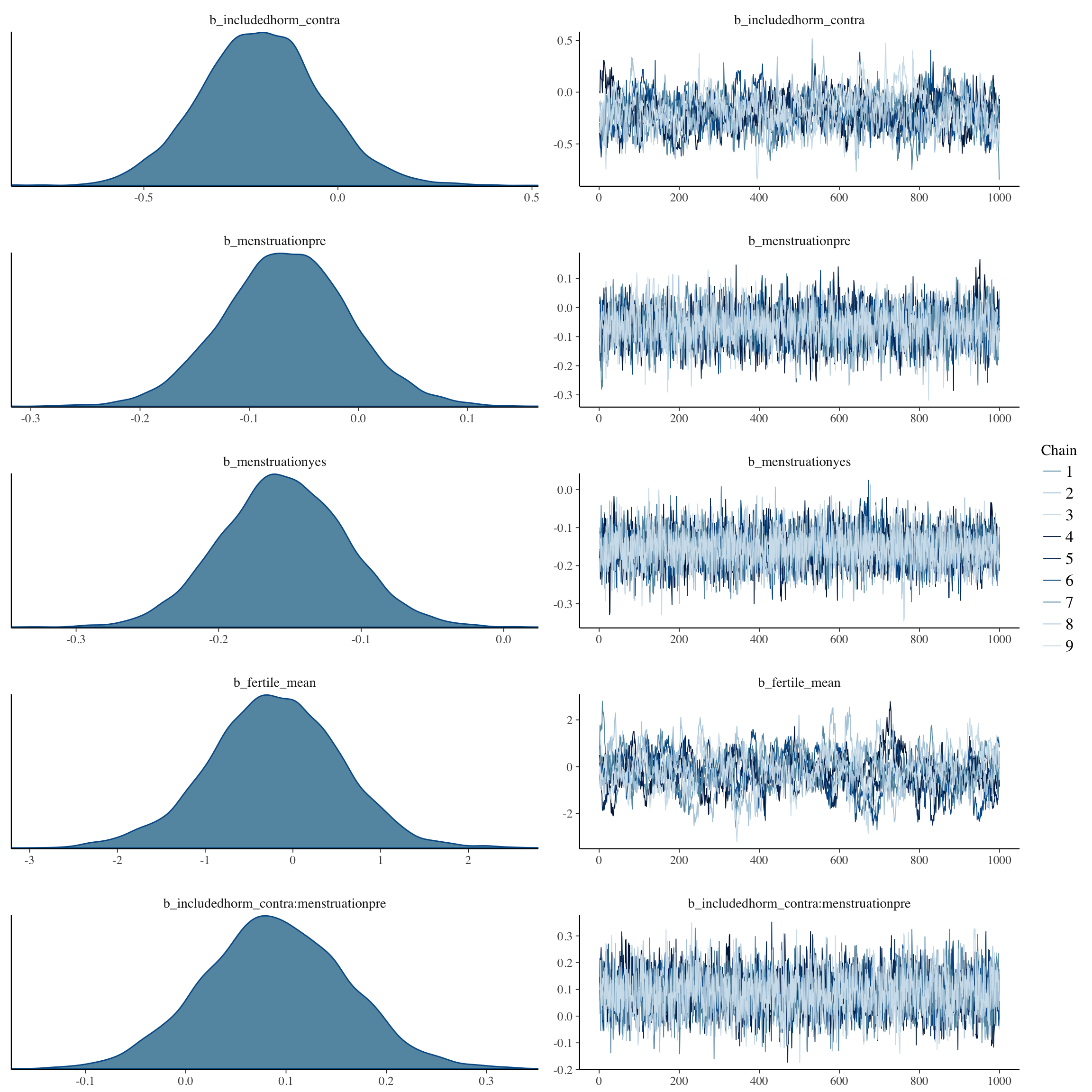
plot(long_rcd, type='coef')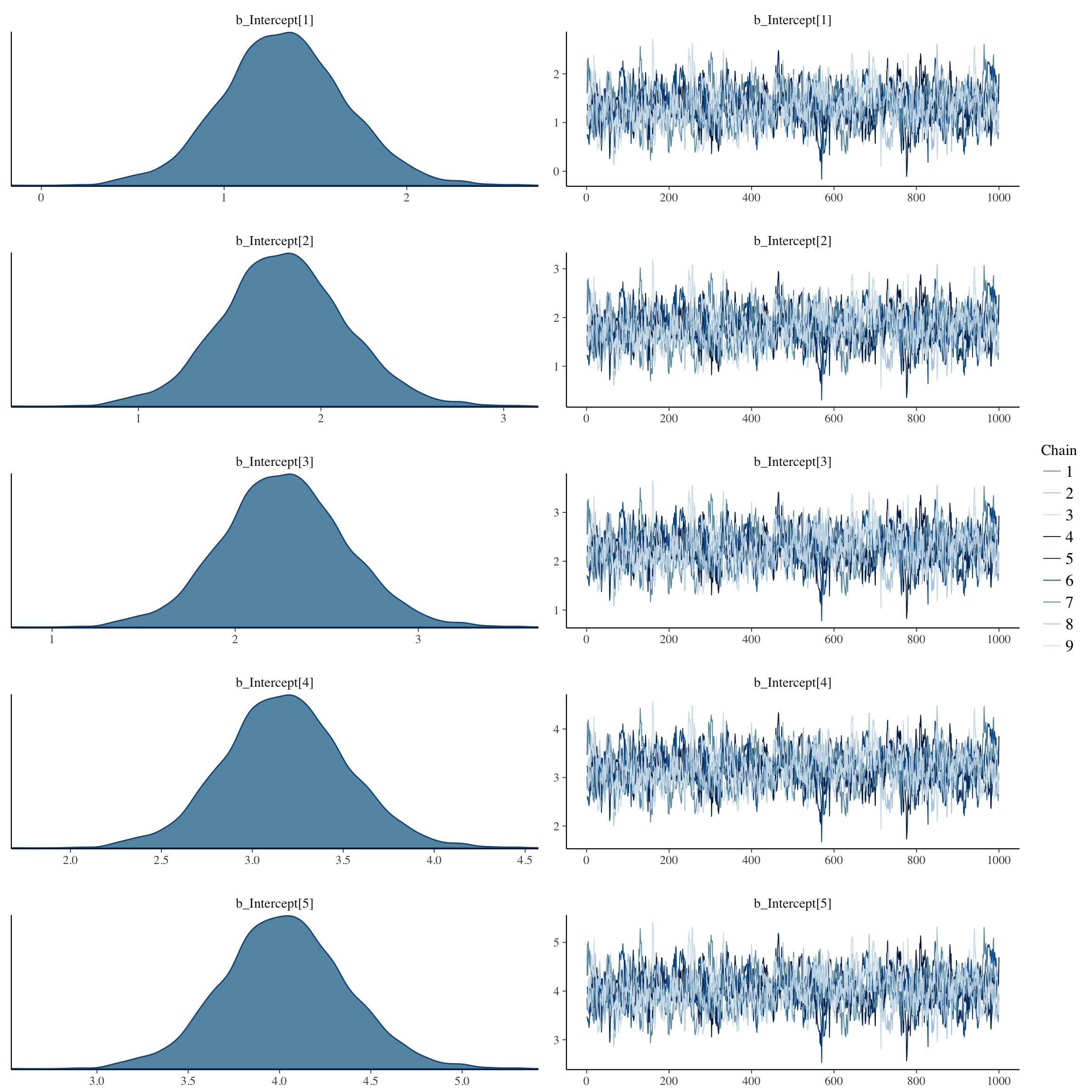
brms::pp_check(long_rcd, re_formula = NA, type = "dens_overlay")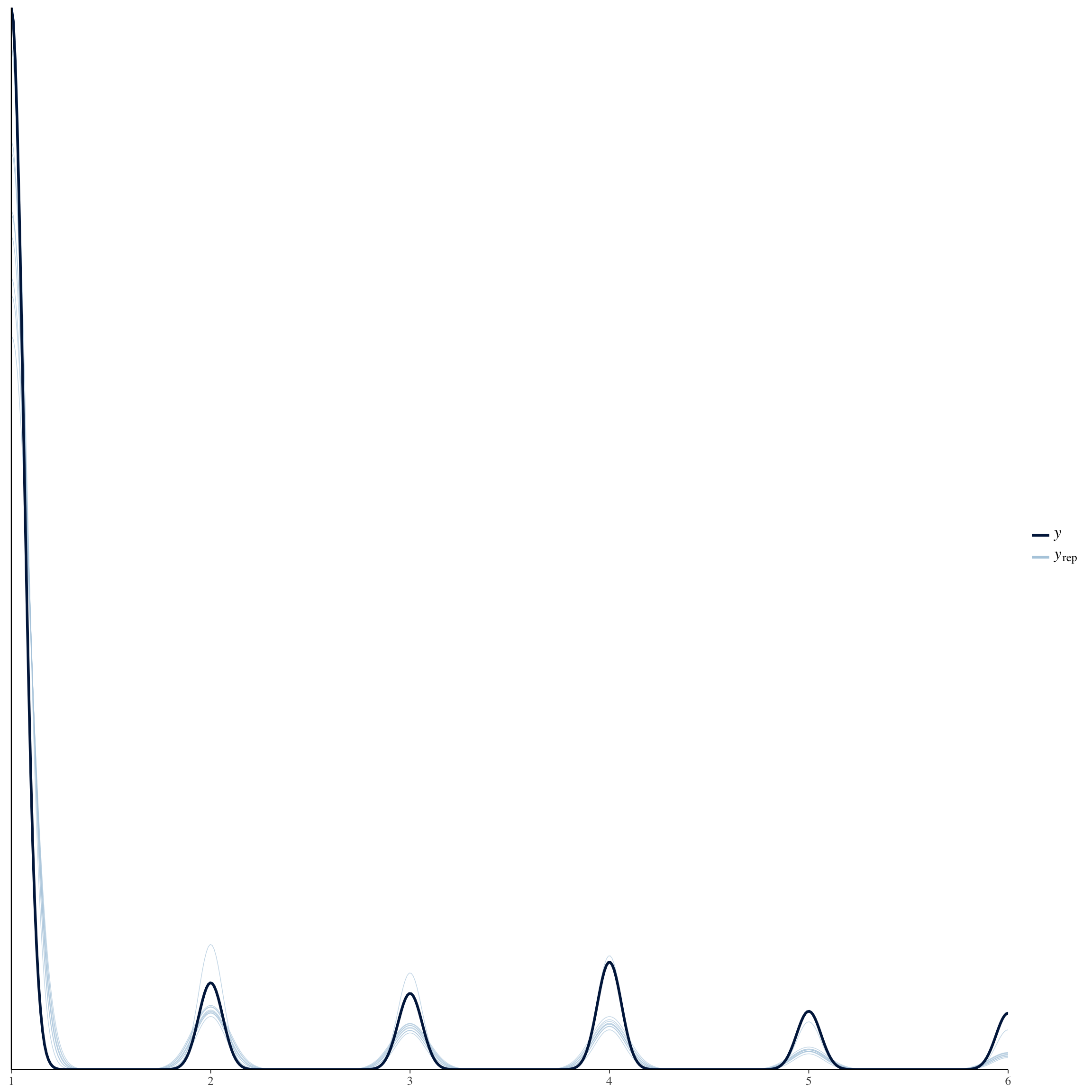
Splines BC, not adjusted
Splines over backward-counted cycle days, not adjusting for menstruation.
Model summary
no_mens = readRDS("3_brms_extra_pair_long_rcd_no_mens.rds")
summary(no_mens)
## Family: cumulative(logit)
## Formula: value ~ included + s(RCD_inferred, by = included) + fertile_mean + (1 | person) + (1 + included | variable)
## disc = 1
## Data: diary_long (Number of observations: 169380)
## Samples: 6 chains, each with iter = 1500; warmup = 500; thin = 1;
## total post-warmup samples = 6000
## ICs: LOO = 285311.81; WAIC = Not computed
##
## Smooth Terms:
## Estimate Est.Error l-95% CI u-95% CI Eff.Sample Rhat
## sds(sRCD_inferredincludedcycling_1) 0.86 0.39 0.39 1.86 1982 1.00
## sds(sRCD_inferredincludedhorm_contra_1) 1.26 0.64 0.44 2.85 1243 1.01
##
## Group-Level Effects:
## ~person (Number of levels: 723)
## Estimate Est.Error l-95% CI u-95% CI Eff.Sample Rhat
## sd(Intercept) 1.28 0.04 1.21 1.36 307 1.04
##
## ~variable (Number of levels: 12)
## Estimate Est.Error l-95% CI u-95% CI Eff.Sample Rhat
## sd(Intercept) 1.00 0.25 0.64 1.61 1198 1
## sd(includedhorm_contra) 0.41 0.11 0.26 0.66 1389 1
## cor(Intercept,includedhorm_contra) 0.23 0.27 -0.33 0.70 1247 1
##
## Population-Level Effects:
## Estimate Est.Error l-95% CI u-95% CI Eff.Sample Rhat
## Intercept[1] 1.32 0.32 0.68 1.98 443 1.01
## Intercept[2] 1.79 0.32 1.15 2.44 443 1.01
## Intercept[3] 2.26 0.32 1.62 2.92 443 1.01
## Intercept[4] 3.17 0.32 2.53 3.83 443 1.01
## Intercept[5] 4.02 0.32 3.38 4.68 443 1.01
## includedhorm_contra -0.18 0.15 -0.48 0.12 306 1.01
## fertile_mean -0.23 0.75 -1.78 1.22 343 1.01
## sRCD_inferred:includedcycling_1 -0.04 0.17 -0.35 0.30 2511 1.00
## sRCD_inferred:includedhorm_contra_1 0.17 0.29 -0.27 0.87 1252 1.00
##
## Samples were drawn using sampling(NUTS). For each parameter, Eff.Sample
## is a crude measure of effective sample size, and Rhat is the potential
## scale reduction factor on split chains (at convergence, Rhat = 1).Marginal effect plots
# by_item = items %>% select(Item.name, Item) %>% unique()
# rownames(by_item) = by_item$Item
# marge = plot(marginal_effects(no_mens, re_formula = ~ (1 + included * menstruation | variable), conditions = by_item), plot = F)
# marge$`RCD_inferred:included` = marge$`RCD_inferred:included` + scale_x_reverse(limits = c(30,0)) + facet_wrap(~ cond__, scales = "free_y")
# marge

smo = marginal_smooths(no_mens)
smo2 = smo$`mu: s(RCD_inferred,by=included)` %>% mutate(included = as.character(included)) %>% bind_rows(
  diary %>% mutate(
    RCD_inferred = -1*RCD, included = 'conc',estimate__ = prc_stirn_b/1.2 - 0.25) %>%
    select(included, RCD_inferred, estimate__) %>%
    filter(RCD_inferred < 30 ) %>% unique())
ggplot(smo2, aes(RCD_inferred, estimate__, color = included, fill = included, linetype = included)) +
  geom_ribbon(aes(ymin = lower__, ymax = upper__), alpha = 0.2, color = NA) +
  geom_line(size = 0.8, stat = "identity") +
  scale_color_manual("", values = c("horm_contra" = "black", "cycling" = "red", "conc" = "#a83fbf"), labels = c("horm_contra"="hormonal contraception user","1"="naturally cycling", "conc" = "superimposed conception risk"))+
  scale_fill_manual("", values = c("horm_contra" = "black", "cycling" = "red", "conc" = "#a83fbf"), labels = c("horm_contra"="hormonal contraception user","1"="naturally cycling", "conc" = "superimposed conception risk")) +
  scale_linetype_manual(values = c("horm_contra" = "solid", "cycling" = "solid", "conc" = "dashed"), guide = F) +
  scale_x_reverse() +
  coord_cartesian(xlim = c(0,30), ylim = c(-0.25, 0.25))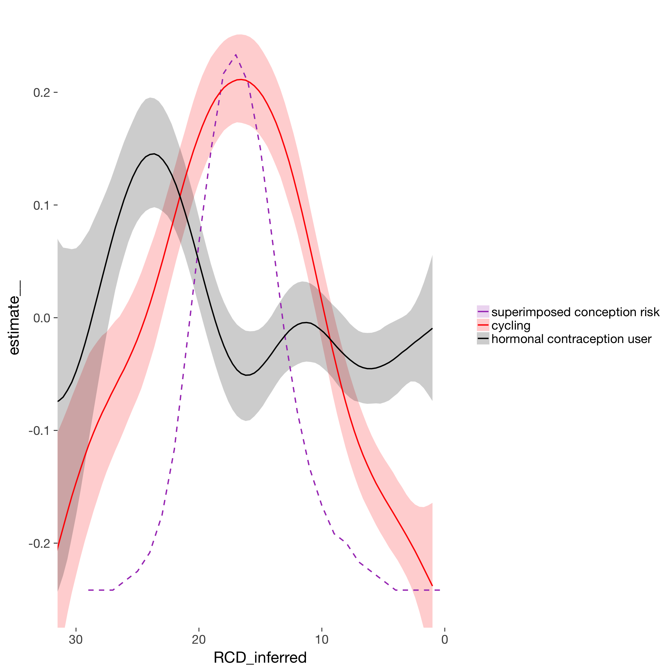
Coefficient plots
bayesplot::mcmc_areas(as.matrix(no_mens$fit), regex_pars = "b_[^I]")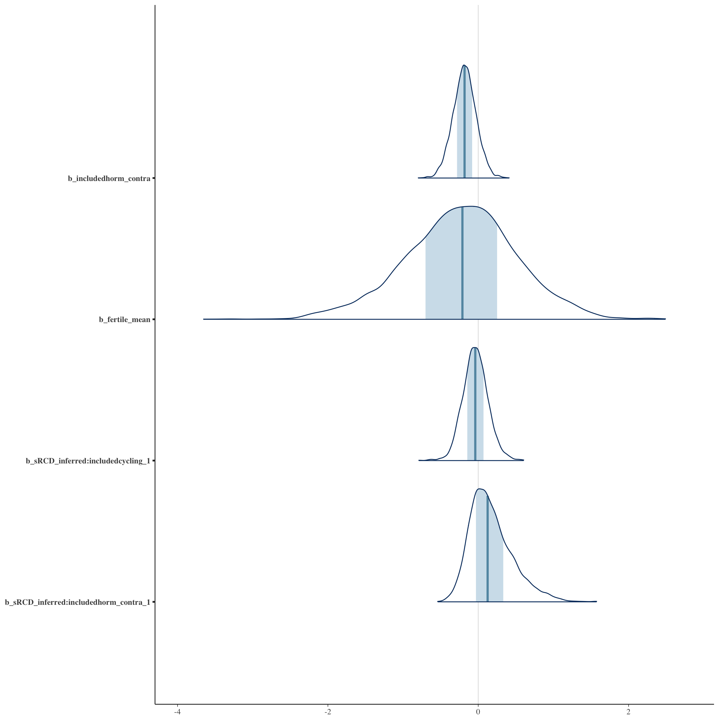
Diagnostic plots
plot(no_mens, type='coef')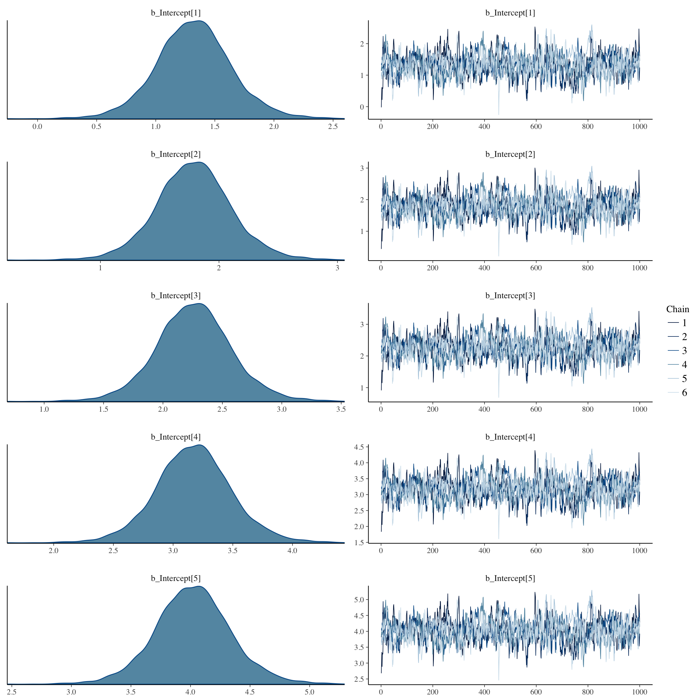
brms::pp_check(no_mens, re_formula = NA, type = "dens_overlay")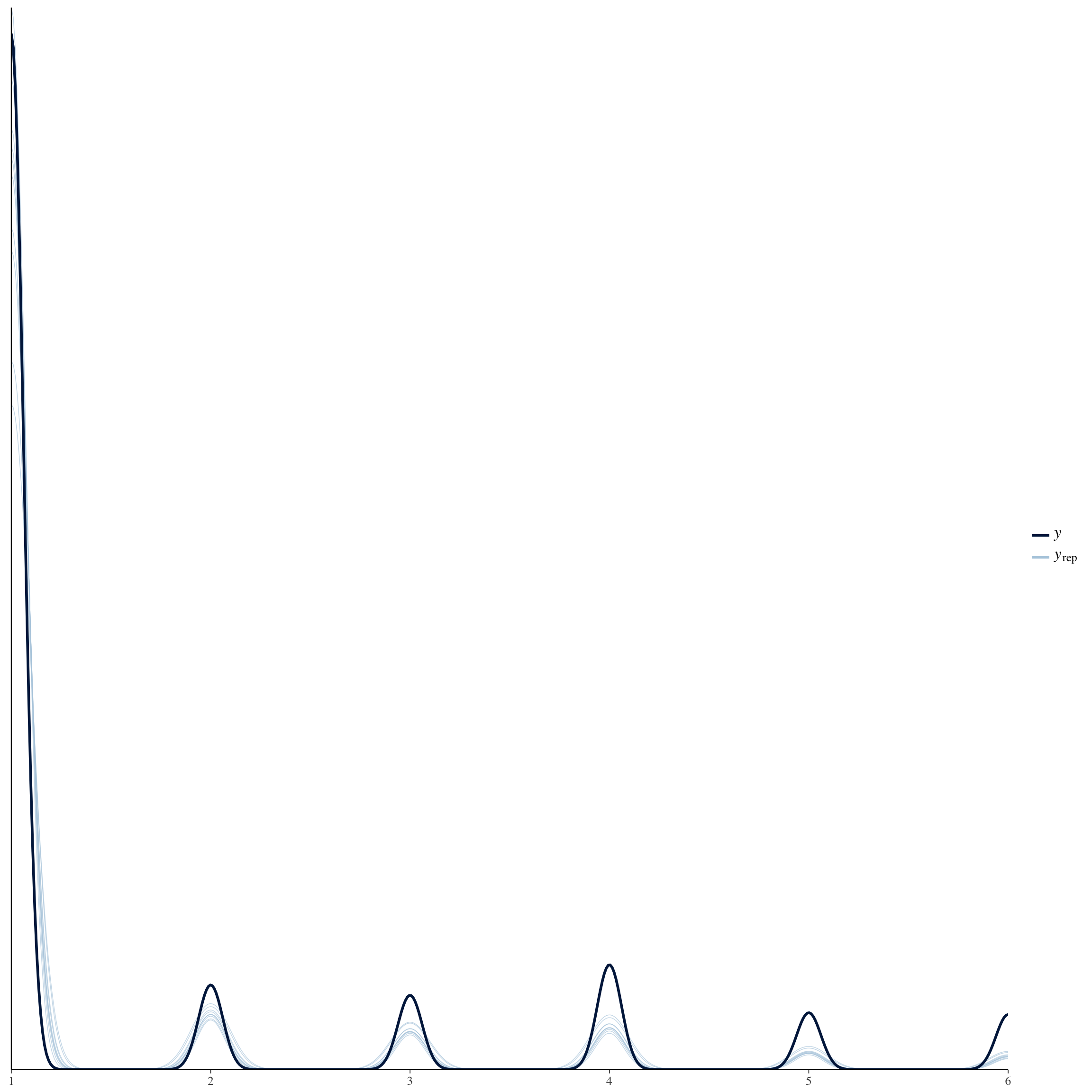
Model comparison
LOO(no_mens, long_rcd, compare = T)## LOOIC SE
## no_mens 285311.81 909.84
## long_rcd 285281.18 909.83
## no_mens - long_rcd 30.63 13.05Marginal effect plots by variable
long_by_i_p = readRDS("3_brms_extra_pair_long_fab_by_item_person.rds")
summary(long_by_i_p)
## Family: cumulative(logit)
## Formula: value ~ included * (menstruation + fertile) + fertile_mean + (1 + menstruation + fertile | person) + (1 + included * (menstruation + fertile) | variable)
## disc = 1
## Data: diary_long (Number of observations: 318528)
## Samples: 5 chains, each with iter = 1500; warmup = 1000; thin = 1;
## total post-warmup samples = 2500
## ICs: LOO = 527142.38; WAIC = Not computed
##
## Group-Level Effects:
## ~person (Number of levels: 1043)
## Estimate Est.Error l-95% CI u-95% CI Eff.Sample Rhat
## sd(Intercept) 1.33 0.03 1.27 1.39 407 1.00
## sd(menstruationpre) 0.66 0.03 0.61 0.71 1086 1.00
## sd(menstruationyes) 0.72 0.03 0.66 0.77 905 1.01
## sd(fertile) 1.49 0.06 1.38 1.60 632 1.01
## cor(Intercept,menstruationpre) -0.19 0.05 -0.29 -0.10 977 1.01
## cor(Intercept,menstruationyes) -0.19 0.05 -0.28 -0.10 728 1.01
## cor(menstruationpre,menstruationyes) 0.52 0.04 0.44 0.60 459 1.01
## cor(Intercept,fertile) -0.25 0.04 -0.34 -0.17 1034 1.00
## cor(menstruationpre,fertile) 0.43 0.04 0.34 0.52 445 1.01
## cor(menstruationyes,fertile) 0.46 0.04 0.37 0.54 296 1.03
##
## ~variable (Number of levels: 12)
## Estimate Est.Error l-95% CI
## sd(Intercept) 1.02 0.26 0.66
## sd(includedhorm_contra) 0.33 0.08 0.22
## sd(menstruationpre) 0.08 0.03 0.03
## sd(menstruationyes) 0.04 0.02 0.00
## sd(fertile) 0.14 0.05 0.05
## sd(includedhorm_contra:menstruationpre) 0.03 0.03 0.00
## sd(includedhorm_contra:menstruationyes) 0.09 0.04 0.02
## sd(includedhorm_contra:fertile) 0.07 0.05 0.00
## cor(Intercept,includedhorm_contra) 0.21 0.23 -0.26
## cor(Intercept,menstruationpre) 0.25 0.26 -0.29
## cor(includedhorm_contra,menstruationpre) 0.34 0.24 -0.17
## cor(Intercept,menstruationyes) 0.05 0.31 -0.57
## cor(includedhorm_contra,menstruationyes) 0.25 0.30 -0.40
## cor(menstruationpre,menstruationyes) 0.20 0.32 -0.47
## cor(Intercept,fertile) 0.18 0.26 -0.36
## cor(includedhorm_contra,fertile) -0.39 0.24 -0.79
## cor(menstruationpre,fertile) -0.20 0.28 -0.71
## cor(menstruationyes,fertile) -0.11 0.31 -0.67
## cor(Intercept,includedhorm_contra:menstruationpre) -0.07 0.34 -0.68
## cor(includedhorm_contra,includedhorm_contra:menstruationpre) -0.13 0.33 -0.71
## cor(menstruationpre,includedhorm_contra:menstruationpre) -0.14 0.34 -0.73
## cor(menstruationyes,includedhorm_contra:menstruationpre) -0.05 0.33 -0.65
## cor(fertile,includedhorm_contra:menstruationpre) 0.03 0.32 -0.60
## cor(Intercept,includedhorm_contra:menstruationyes) 0.06 0.28 -0.49
## cor(includedhorm_contra,includedhorm_contra:menstruationyes) 0.45 0.25 -0.16
## cor(menstruationpre,includedhorm_contra:menstruationyes) 0.08 0.29 -0.49
## cor(menstruationyes,includedhorm_contra:menstruationyes) 0.04 0.31 -0.56
## cor(fertile,includedhorm_contra:menstruationyes) -0.11 0.29 -0.63
## cor(includedhorm_contra:menstruationpre,includedhorm_contra:menstruationyes) -0.04 0.33 -0.67
## cor(Intercept,includedhorm_contra:fertile) 0.14 0.33 -0.54
## cor(includedhorm_contra,includedhorm_contra:fertile) 0.13 0.32 -0.53
## cor(menstruationpre,includedhorm_contra:fertile) 0.18 0.32 -0.49
## cor(menstruationyes,includedhorm_contra:fertile) 0.08 0.33 -0.58
## cor(fertile,includedhorm_contra:fertile) -0.20 0.33 -0.78
## cor(includedhorm_contra:menstruationpre,includedhorm_contra:fertile) 0.04 0.32 -0.59
## cor(includedhorm_contra:menstruationyes,includedhorm_contra:fertile) 0.11 0.33 -0.55
## u-95% CI Eff.Sample Rhat
## sd(Intercept) 1.70 656 1.01
## sd(includedhorm_contra) 0.52 1006 1.01
## sd(menstruationpre) 0.16 1293 1.00
## sd(menstruationyes) 0.09 1258 1.00
## sd(fertile) 0.26 1788 1.00
## sd(includedhorm_contra:menstruationpre) 0.10 2007 1.00
## sd(includedhorm_contra:menstruationyes) 0.17 1461 1.00
## sd(includedhorm_contra:fertile) 0.19 1529 1.00
## cor(Intercept,includedhorm_contra) 0.61 1051 1.00
## cor(Intercept,menstruationpre) 0.70 2500 1.00
## cor(includedhorm_contra,menstruationpre) 0.75 2047 1.00
## cor(Intercept,menstruationyes) 0.63 2500 1.00
## cor(includedhorm_contra,menstruationyes) 0.76 2500 1.00
## cor(menstruationpre,menstruationyes) 0.75 2500 1.00
## cor(Intercept,fertile) 0.64 2500 1.00
## cor(includedhorm_contra,fertile) 0.12 2500 1.00
## cor(menstruationpre,fertile) 0.37 2500 1.00
## cor(menstruationyes,fertile) 0.51 1770 1.00
## cor(Intercept,includedhorm_contra:menstruationpre) 0.59 2500 1.00
## cor(includedhorm_contra,includedhorm_contra:menstruationpre) 0.55 2500 1.00
## cor(menstruationpre,includedhorm_contra:menstruationpre) 0.53 2500 1.00
## cor(menstruationyes,includedhorm_contra:menstruationpre) 0.58 2500 1.00
## cor(fertile,includedhorm_contra:menstruationpre) 0.64 2500 1.00
## cor(Intercept,includedhorm_contra:menstruationyes) 0.58 2500 1.00
## cor(includedhorm_contra,includedhorm_contra:menstruationyes) 0.84 2500 1.00
## cor(menstruationpre,includedhorm_contra:menstruationyes) 0.63 2500 1.00
## cor(menstruationyes,includedhorm_contra:menstruationyes) 0.66 2500 1.00
## cor(fertile,includedhorm_contra:menstruationyes) 0.48 2500 1.00
## cor(includedhorm_contra:menstruationpre,includedhorm_contra:menstruationyes) 0.58 2030 1.00
## cor(Intercept,includedhorm_contra:fertile) 0.73 2500 1.00
## cor(includedhorm_contra,includedhorm_contra:fertile) 0.70 2500 1.00
## cor(menstruationpre,includedhorm_contra:fertile) 0.75 2500 1.00
## cor(menstruationyes,includedhorm_contra:fertile) 0.67 2500 1.00
## cor(fertile,includedhorm_contra:fertile) 0.49 2500 1.00
## cor(includedhorm_contra:menstruationpre,includedhorm_contra:fertile) 0.65 1587 1.00
## cor(includedhorm_contra:menstruationyes,includedhorm_contra:fertile) 0.70 2500 1.00
##
## Population-Level Effects:
## Estimate Est.Error l-95% CI u-95% CI Eff.Sample Rhat
## Intercept[1] 1.33 0.31 0.75 1.96 498 1.01
## Intercept[2] 1.78 0.31 1.20 2.41 498 1.01
## Intercept[3] 2.25 0.31 1.67 2.88 498 1.01
## Intercept[4] 3.17 0.31 2.60 3.81 497 1.01
## Intercept[5] 4.00 0.31 3.42 4.64 498 1.01
## includedhorm_contra -0.29 0.14 -0.56 -0.01 246 1.02
## menstruationpre -0.24 0.05 -0.35 -0.14 862 1.00
## menstruationyes -0.20 0.05 -0.29 -0.10 652 1.00
## fertile 0.25 0.11 0.05 0.46 953 1.00
## fertile_mean 0.03 0.43 -0.83 0.83 481 1.01
## includedhorm_contra:menstruationpre 0.15 0.06 0.04 0.27 903 1.00
## includedhorm_contra:menstruationyes 0.18 0.06 0.06 0.31 806 1.00
## includedhorm_contra:fertile -0.28 0.13 -0.54 -0.04 705 1.01
##
## Samples were drawn using sampling(NUTS). For each parameter, Eff.Sample
## is a crude measure of effective sample size, and Rhat is the potential
## scale reduction factor on split chains (at convergence, Rhat = 1).newd = diary_long %>% select(included, fertile, variable) %>% unique()
newd$fertile_mean = 0.1
newd$menstruation = diary$menstruation[3]
# newd$value = 1
# newd$person = 10
# newd$day_number = 1
predicted = fitted(long_by_i_p, newdata = newd, re_formula = ~ (1 + fertile | variable), summary = F)
multiply_by_level = rep(sort(unique(long_by_i_p$data$value)), each = dim(predicted)[1] * dim(predicted)[2])
dim(multiply_by_level) = dim(predicted)
predicted = predicted * multiply_by_level
response = apply(predicted, MARGIN = c(1:2), FUN = sum)
newd$Estimate = apply(response, MARGIN = 2, FUN = mean)
intervals = apply(response, MARGIN = 2, FUN = function(x) { quantile(x, probs = c(0.025,0.975)) })
newd$lower = unlist(intervals[1, ])
newd$upper = unlist(intervals[2, ])
vartolabel = "'extra_pair_2'='wichtig, dass mich andere Männer als attraktiv wahrnehmen.';
'extra_pair_3'='Komplimente von anderen Männern erhalten.';
'extra_pair_4'='via Medien mit Freunden, Bekannten oder Kollegen geflirtet.';
'extra_pair_5'='ohne meinen Partner ausgegangen.';
'extra_pair_6'='ohne meinen Partner an einen Ort gegangen, wo man Männer treffen kann.';
'extra_pair_7'='mir Gedanken über einen anderen potentiellen Partner gemacht.';
'extra_pair_8'='mit Männern geflirtet, die ich nicht kannte.';
'extra_pair_9'='mit Freunden, Kollegen oder Bekannten geflirtet.';
'extra_pair_10'='mich zu einem Freund, Bekannten oder Kollegen hingezogen gefühlt';
'extra_pair_11'='mich zu einem Mann hingezogen gefühlt, den ich nicht kannte.';
'extra_pair_12'='sind mir attraktive Männer in meiner Umgebung aufgefallen.';
'extra_pair_13'='sexuelle Fantasien mit anderen Männern als meinem Partner.';
'desirability_1'='habe ich mich sexuell begehrenswert gefühlt.';
'desirability_partner'='fand ich meinen Partner besonders sexuell anziehend.';
'sexual_intercourse_1'='Lust, mit Ihrem Partner Geschlechtsverkehr zu haben'"
vartolabel = "'extra_pair_2'='important that other men find me attractive';
'extra_pair_3'='received compliments from other men';
'extra_pair_4'='flirted with friends, acquaintances or colleagues via media';
'extra_pair_5'='went out without my partner';
'extra_pair_6'='went to a place where one can meet men without my partner';
'extra_pair_7'='thought about a different potential partner';
'extra_pair_8'='flirted with men I didn\\'t know';
'extra_pair_9'='flirted with friends, acquaintances or colleagues';
'extra_pair_10'='felt attracted to a friend, acquaintance or colleague';
'extra_pair_11'='felt attracted to a man I didn\\'t know';
'extra_pair_12'='noticed attractive men around me';
'extra_pair_13'='had sexual fantasies about men other than my partner';
'desirability_1'='felt sexually desirable';
'desirability_partner'='found my partner particularly sexually attractive';
'sexual_intercourse_1'='wanted to have sex with my partner'"
newd$label = car::Recode(newd$variable, vartolabel)
newd$label = stringr::str_wrap(newd$label, width = 40)Flexible y-axis
ggplot(newd, aes(x = fertile, y = Estimate, colour = included)) +
  geom_smooth(aes(ymin = lower, ymax = upper), stat = "identity",  show.legend = FALSE) +  scale_colour_manual("", values = c("cycling"="red","horm_contra"="black")) +
  facet_wrap(~ label, scales = "free_y", ncol = 3)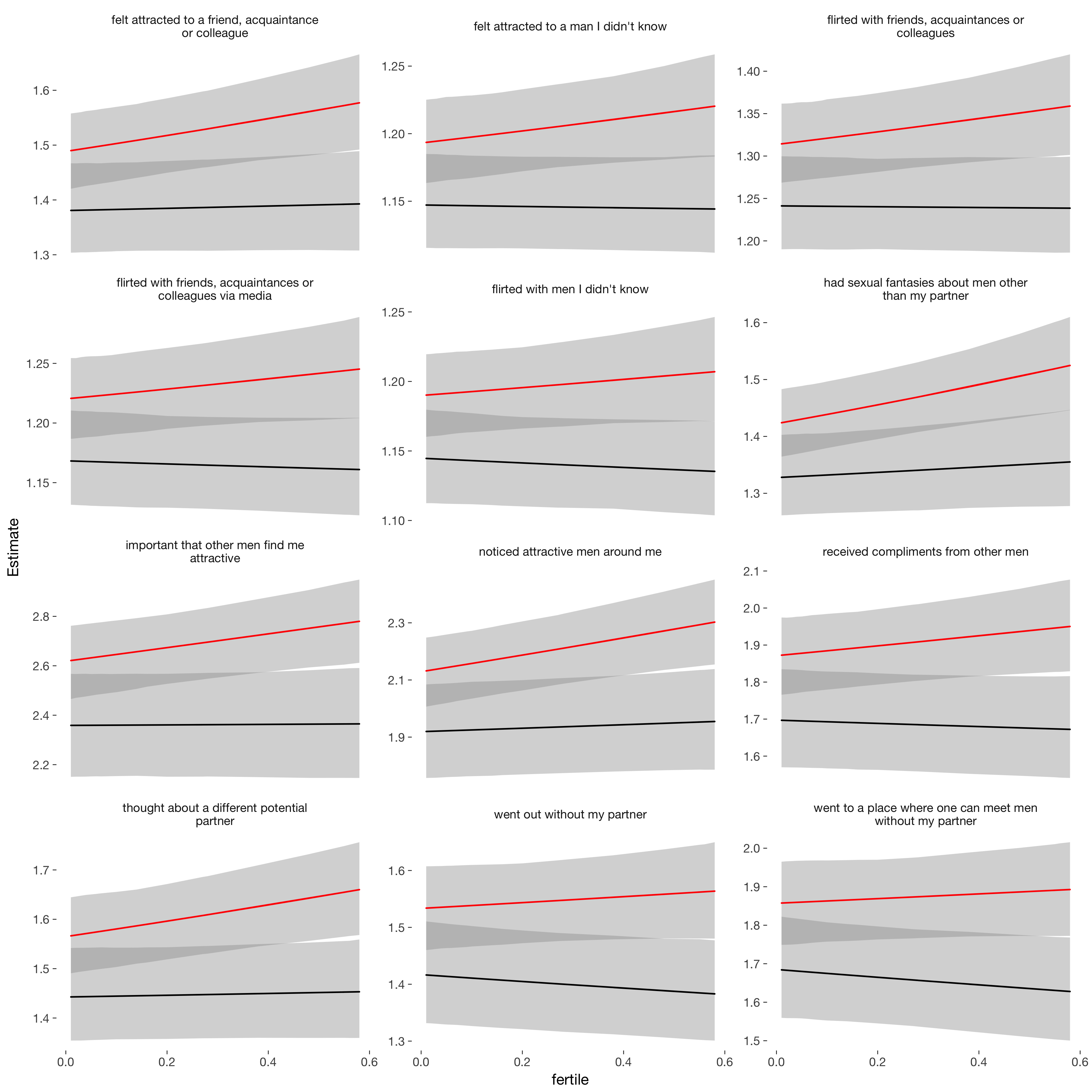
Fixed y-axis
ggplot(newd, aes(x = fertile, y = Estimate, colour = included)) +
  geom_smooth(aes(ymin = lower, ymax = upper), stat = "identity",  show.legend = FALSE) +  scale_colour_manual("", values = c("cycling"="red","horm_contra"="black")) +
  facet_wrap(~ label, ncol = 3)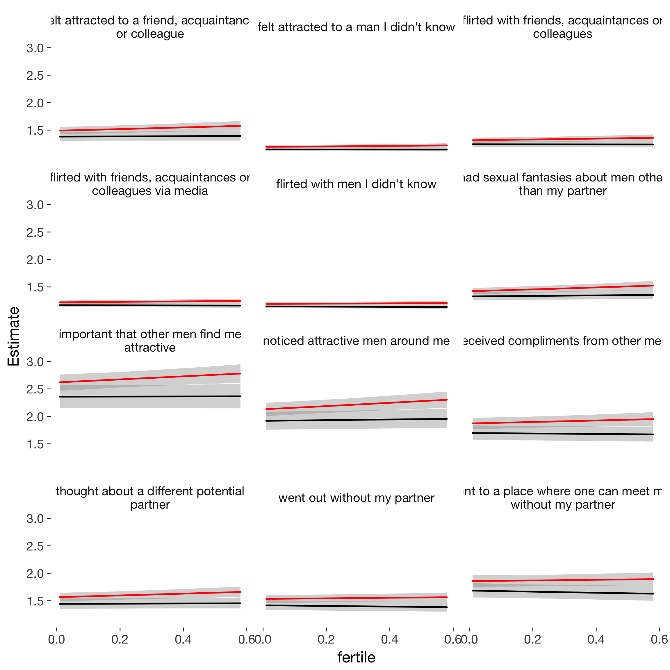
Table
fixefs = broom::tidy(long_by_i_p)
by_var = ranef(long_by_i_p)$variable
fertile_by_var = by_var[,,"fertile"] %>% data.frame(check.names = F) %>%  tibble::rownames_to_column("variable") %>%
  mutate(mean = fixefs %>% filter(term=='b_fertile') %>% .[["estimate"]])
hc_fertile_by_var = by_var[,,"includedhorm_contra:fertile"] %>% data.frame(check.names = F) %>%  tibble::rownames_to_column("variable") %>% mutate(mean = fixefs %>% filter(term=='b_includedhorm_contra:fertile') %>% .[["estimate"]])
fertile_by_var = bind_rows(cycling = fertile_by_var, `HC user` = hc_fertile_by_var, .id = "included")

fertile_by_var$label = stringr::str_wrap(car::Recode(fertile_by_var$variable, vartolabel), width = 40)
ggplot(fertile_by_var, aes(x = label, y = Estimate + mean, ymin = `2.5%ile` + mean, ymax = `97.5%ile` + mean, color = included)) +
  geom_pointrange(position = position_dodge(width = 0.5)) +
  coord_flip() +
  scale_color_manual(values = c("cycling" = "red", "HC user" = "black")) +
  geom_hline(aes(yintercept = mean, group = included, color = included), linetype = 'dashed')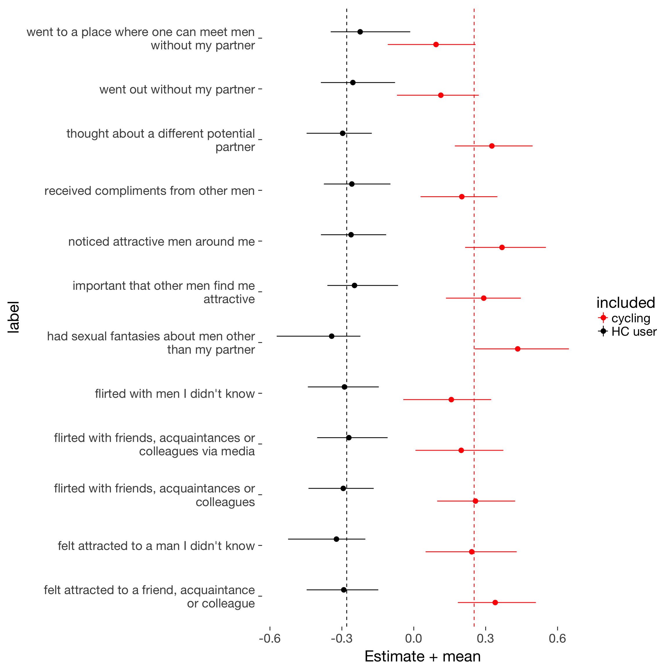
Marginal effects by person
rand500 = sample(unique(long_by_i_p$data$person), size = 200)
newd = unique(long_by_i_p$data[, c("included", "fertile", "person")]) %>% filter(person %in% rand500)
newd$fertile_mean = 0.1
newd$menstruation = diary$menstruation[3]
predicted = fitted(long_by_i_p, newdata = newd, re_formula = ~ (1 + fertile  | person), summary = F)

multiply_by_level = rep(1:dim(predicted)[3], each = dim(predicted)[1] * dim(predicted)[2])
dim(multiply_by_level) = dim(predicted)
predicted = predicted * multiply_by_level
response = apply(predicted, MARGIN = c(1:2), FUN = sum)
newd$Estimate = apply(response, MARGIN = 2, FUN = mean)
newd$Estimate = apply(response, MARGIN = 2, FUN = mean)
intervals = apply(response, MARGIN = 2, FUN = function(x) { quantile(x, probs = c(0.025,0.975)) })
newd$lower = unlist(intervals[1, ])
newd$upper = unlist(intervals[2, ])

newd %>% arrange(person, fertile) -> newd
newd$Estimate2 = newd$Estimate - ave(newd$Estimate, newd$person, FUN = function(x) { head(x,1) })

ggplot(newd, aes(x = fertile, y = Estimate2, colour = included)) +
  geom_line(aes(group = person), alpha = 0.05, stat = "identity",  show.legend = FALSE) +
  scale_colour_manual("", values = c("cycling"="red","horm_contra"="black")) +
  facet_wrap(~ included) +
  geom_line(stat = 'smooth', method = 'lm', size = 1, show.legend = FALSE) +
  ggtitle("Individual differences in ovulatory shifts") +
  ylab("Shift (across outcomes)")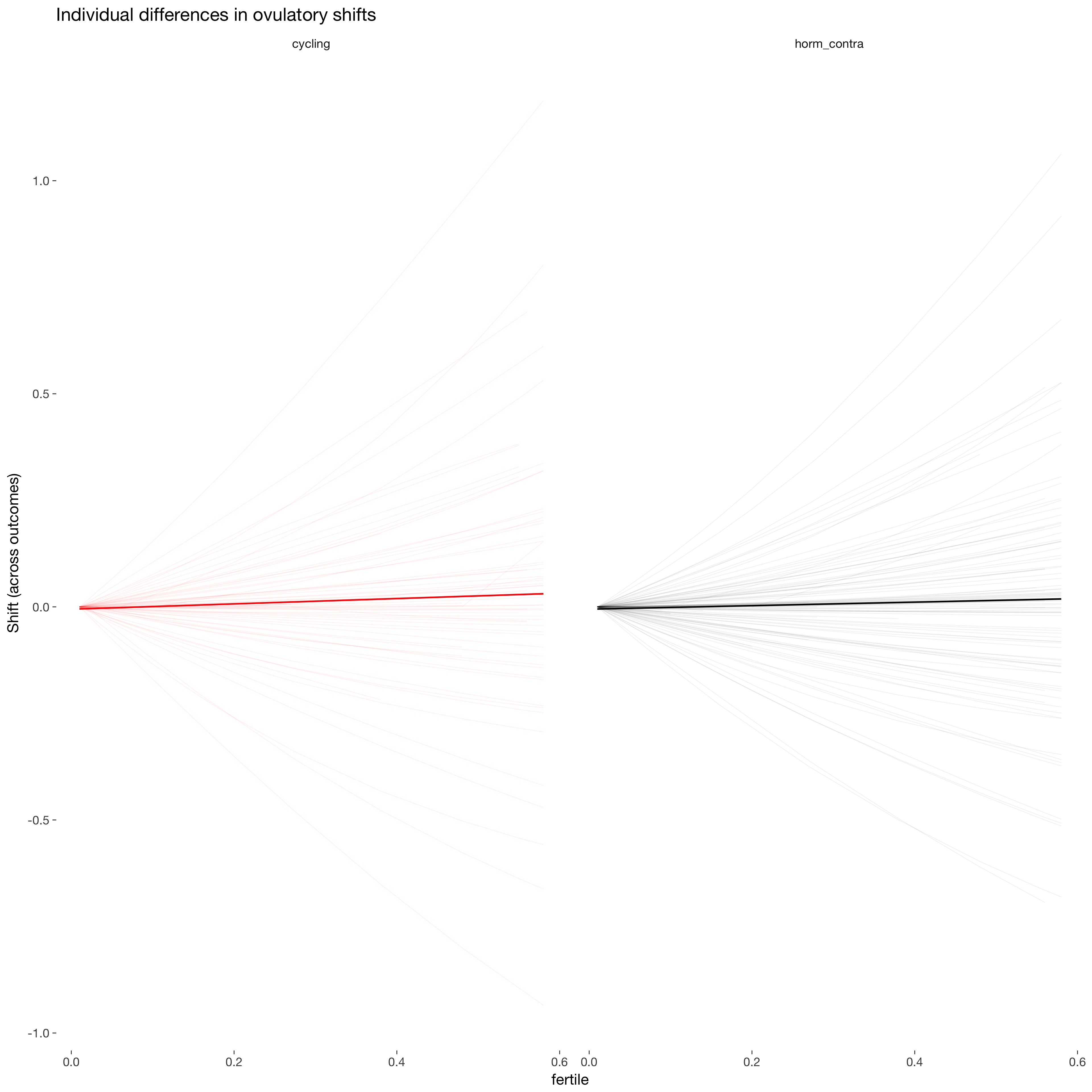
Item-level raw means over cycle days
theme_henrik <- function(grid=TRUE, legend.position=NA) {
th <- ggplot2::theme_minimal(base_size = 12)
th <- th + theme(text = element_text(color='#333333'))
th <- th + theme(legend.background = element_blank())
th <- th + theme(legend.key = element_blank())
# Straight out of hrbrthemes
if (inherits(grid, "character") | grid == TRUE) {
th <- th + theme(panel.grid=element_line(color="#cccccc", size=0.3))
th <- th + theme(panel.grid.major=element_line(color="#cccccc", size=0.3))
th <- th + theme(panel.grid.minor=element_line(color="#cccccc", size=0.15))
if (inherits(grid, "character")) {
if (regexpr("X", grid)[1] < 0) th <- th + theme(panel.grid.major.x=element_blank())
if (regexpr("Y", grid)[1] < 0) th <- th + theme(panel.grid.major.y=element_blank())
if (regexpr("x", grid)[1] < 0) th <- th + theme(panel.grid.minor.x=element_blank())
if (regexpr("y", grid)[1] < 0) th <- th + theme(panel.grid.minor.y=element_blank())
}
} else {
th <- th + theme(panel.grid=element_blank())
}
th <- th + theme(axis.text = element_text())
th <- th + theme(axis.ticks = element_blank())
th <- th + theme(axis.text.x=element_text(margin=margin(t=0.5)))
th <- th + theme(axis.text.y=element_text(margin=margin(r=0.5)))
th <- th + theme(plot.title = element_text(),
plot.subtitle = element_text(margin=margin(b=15)),
plot.caption = element_text(face='italic', size=10))
if (!is.na(legend.position)) th <- th + theme(legend.position = legend.position)
return (th)
}
diary %>% group_by(person) %>%
filter(!is.na(fertile_fab), !is.na(included_all),
RCD > -1 * minimum_cycle_length_diary, RCD > -29) %>%
filter(!is.na(included_all), !is.na(fertile_fab)) %>%
mutate(included = included_all,
fertile_mean = mean(fertile_fab, na.rm = T)) %>%
select(person, n_days, menstruation, RCD_inferred, fertile_mean, fertile_fab, included, extra_pair_2, extra_pair_3, extra_pair_4, extra_pair_5, extra_pair_6, extra_pair_7, extra_pair_8, extra_pair_9, extra_pair_10, extra_pair_11, extra_pair_12, extra_pair_13, desirability_partner, desirability_1, sexual_intercourse_1, attention_2
# ,extra_pair, in_pair_desire
) %>%
tidyr::gather(variable, value, -person, -menstruation, -fertile_mean, -fertile_fab, -included, -RCD_inferred, -n_days) %>%
left_join(items %>% select(Item.name, Item), by = c("variable" = "Item.name")) %>%
mutate(RCD_inferred = -1* RCD_inferred + 1, variable = factor(str_wrap(str_sub(Item,4),40))) %>%
filter(!is.na(value), RCD_inferred > -29) %>%
group_by(included, person, variable) %>%
mutate(value = value - min(value),
value = value / max(value)) %>%
group_by(included, Item, variable, RCD_inferred) %>%
summarise(value = mean(value, na.rm = T)) %>%
group_by(included, variable) %>%
arrange(RCD_inferred) %>%
mutate(
value_min = value - min(value),
p_peak = value_min / max(value_min), # Normalize as percentage of peak popularity
p_smooth = (
coalesce(lag(p_peak), p_peak[RCD_inferred==0]) + p_peak + coalesce(lead(p_peak), p_peak[RCD_inferred==-28])) / 3 # Moving average, accounting for cyclical nature
) %>% # When there's no lag or lead, we get NA. Use the pointwise data
group_by(included) %>%
mutate(variable = reorder(variable, p_smooth, FUN=which.max)) %>% # order by peak time
arrange(variable) %>%
mutate(variable.f = reorder(as.character(variable), desc(variable))) ->
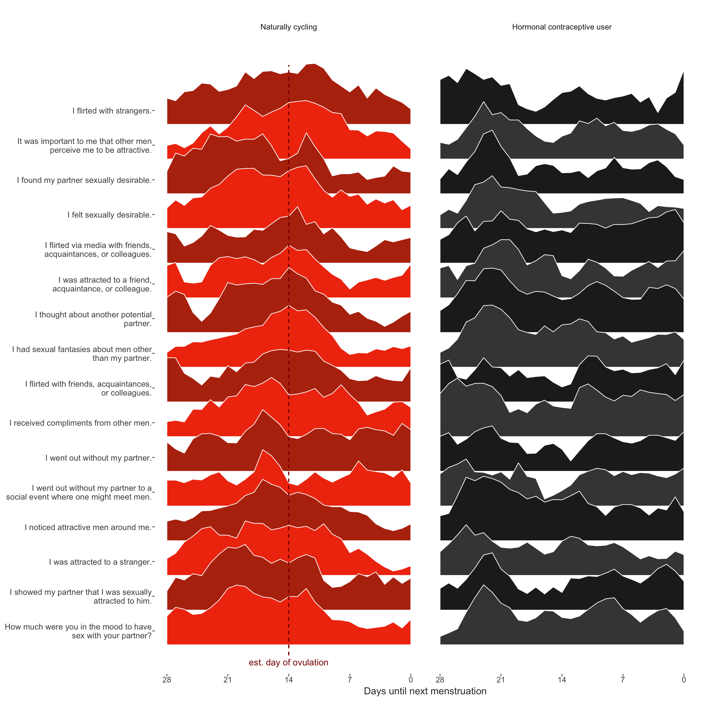
item_timeseriests_plot = item_timeseries %>%
filter(!is.na(included)) %>%
{
items <- levels(.$variable)
ggplot(., aes(x = RCD_inferred, group = variable.f, fill = factor(paste0(included,as.integer(variable.f) %% 2)))) +
geom_ribbon(aes(ymin = as.integer(variable), ymax = as.integer(variable) + 2 * (p_smooth)), color='white', size=0.4) +
scale_x_continuous("Days until next menstruation", breaks = c(-0,-7,-14,-21,-28), labels = c("0","7","14","21","28")) +
# "Re-add" activities by names as labels in the Y scale
scale_y_continuous(breaks = 1:length(items) + 0.4, labels = function(y) {items[y]})+
# Zebra color for readability; will change colors of labels in Inkscape later
scale_fill_manual(values = c('horm_contra0' = '#444444', 'horm_contra1' = '#222222', 'cycling0' = '#F13B0E', 'cycling1' = '#B7320E'))+
ggtitle("") +
theme_henrik(grid='', legend.position='none') +
theme(
axis.ticks.x = element_line(size=0.3),
axis.ticks.y = element_line(size=0.3),
axis.text.y = element_text(size = 10))+
facet_wrap(~ included, labeller = labeller(included = c(`cycling` = 'Naturally cycling', `horm_contra` = 'Hormonal contraceptive user'))) +
geom_segment(aes(x = if_else(included=="cycling",-14,NA_real_), xend = if_else(included=="cycling",-14,NA_real_)), color = 'darkred', linetype = 'dashed', y = 0.7, yend = 17.7)+
geom_text(data = data.frame(included = 'cycling', variable.f = 1, RCD_inferred = -14), label = 'est. day of ovulation', color = 'darkred', y = 0.5)
}
ggsave(ts_plot, file = "item_timeseries.pdf", width = 10, height = 10)
ts_plot