Curve plot

Cycling women (not on hormonal birth control)

Women on hormonal birth control

Load data

library(knitr)
opts_chunk$set(fig.width = 8, fig.height = 8, cache = T, warning = T, message = F, cache = F)

source("0_helpers.R")
load("full_data.rdata")
diary = diary %>% 
  mutate(
  included = included_all,
  fertile = if_else(is.na(prc_stirn_b_squished), prc_stirn_b_backward_inferred, prc_stirn_b_squished)
)  %>% group_by(person) %>% 
  mutate(
      fertile_mean = mean(fertile, na.rm = T)
  ) %>% filter(minimum_cycle_length_diary <= 36, minimum_cycle_length_diary > 20) %>% mutate(fertile=prc_stirn_b)

opts_chunk$set(warning = F)
library(Cairo)
opts_chunk$set(dev = "CairoPNG")

library(ggplot2)

# form a subset and run the model without the hormonal contraception and the fertility predictors
tmp = diary %>%
  filter(!is.na(fertile), !is.na(included),
         RCD > -1 * minimum_cycle_length_diary, RCD > -40) %>% 
  filter(!is.na(RCD))
rcd_min = min(tmp$RCD)

tmp$real = FALSE
tmp_before = tmp
tmp_before$RCD = tmp_before$RCD + min(tmp$RCD) - 1
tmp_after = tmp
tmp_after$RCD = tmp_after$RCD - min(tmp$RCD) + 1
tmp$real = TRUE
tmp = bind_rows(tmp_before %>% filter(RCD > rcd_min - 11), tmp, tmp_after %>% filter(RCD < 11))

GAM smooth on raw data

As before, but without partialling anything out.

extra_pair = ggplot(tmp,aes_string(x = "RCD", y = "extra_pair", colour = "included")) +
    stat_smooth(geom = 'smooth',size = 0.8, fill = "#9ECAE1", method = 'gam', formula = y ~ s(x))

in_pair_desire = ggplot(tmp,aes_string(x = "RCD", y = "in_pair_desire", colour = "included")) +
    stat_smooth(geom = 'smooth',size = 0.8, fill = "#9ECAE1", method = 'gam', formula = y ~ s(x))

desirability_1 = ggplot(tmp,aes_string(x = "RCD", y = "desirability_1", colour = "included")) +
    stat_smooth(geom = 'smooth',size = 0.8, fill = "#9ECAE1", method = 'gam', formula = y ~ s(x))

trend_data = bind_rows(
  extra_pair = ggplot_build(extra_pair)$data[[1]],
  in_pair_desire = ggplot_build(in_pair_desire)$data[[1]],
  desirability_1 = ggplot_build(desirability_1)$data[[1]],
  .id = "outcome"
)

trend_data$RCD = round(trend_data$x)
trend_data = left_join(trend_data, tmp %>% select(real, RCD,fertile) %>% unique(), by = "RCD")
trend_data = bind_rows(trend_data %>%
  filter(group == 1) %>%
  group_by(outcome) %>% 
  mutate(
    group = 3,
    ymin = NA,
    ymax = NA,
    y = ( ( (fertile - 0.01)/0.58) * (max(y)-min(y) ) ) + min(y) ), 
  trend_data) %>% 
  filter(real == TRUE)

trend_data$outcome_label = recode(str_replace_all(str_replace_all(str_replace_all(trend_data$outcome, "_", " "), " pair", "-pair"), " 1", ""), 
                       "desirability" = "self-perceived desirability",
                       "NARQ admiration" = "narcissistic admiration",
                       "NARQ rivalry" = "narcissistic rivalry",
                       "extra-pair" = "extra-pair desire & behaviour",
                       "had sexual intercourse" = "sexual intercourse")

theme_set(theme_tufte(base_size = 16, base_family='Helvetica'))

plot1b = ggplot(trend_data) +
  geom_ribbon(aes(x = x, ymin = ymin, ymax = ymax,  fill = factor(group)), alpha = 0.2) +
  geom_line(aes(x = x, y = y, colour = factor(group), linetype = factor(group)), size = 0.8, stat = "identity") +
  scale_x_continuous("Days until next menstruation") +
  ylab("Outcome (in Likert points)") +
  scale_linetype_manual(values = c("2" = "solid", "1" = "solid", "3" = "dashed"), guide = F) +
  scale_color_manual("", values = c("2" = "black", "1" = "red", "3" = "#a83fbf"), labels = c("2"="hormonal contraception user","1"="naturally cycling", "3" = "fertile window probability")) +
  scale_fill_manual("", values = c("2" = "black", "1" = "red", "3" = "#a83fbf"), labels = c("2"="hormonal contraception user","1"="naturally cycling", "3" = "fertile window probability")) +
  facet_wrap(~ outcome_label, scales = "free_y", ncol = 2) +
  theme(legend.position = c(1,0.1), legend.justification = c(1,0),
        axis.text = element_text(size = 12),
        axis.title = element_text(size = 14))

suppressWarnings(print(plot1b))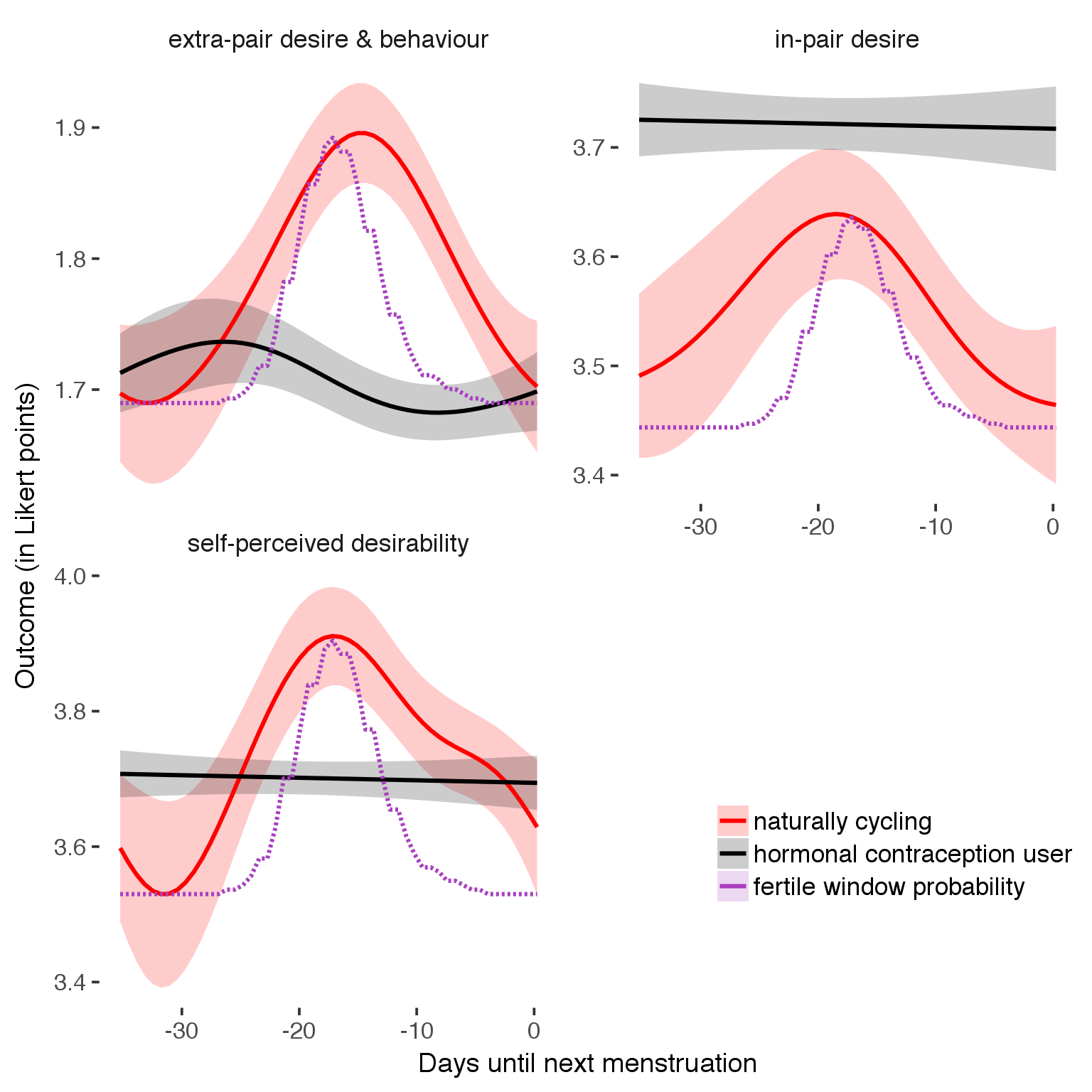

ggsave(plot1b, filename = "_site/library/curves_paper.png", width = 8, height = 7)
ggsave(plot1b, filename = "curves_paper.pdf", width = 8, height = 7)