Item-level analyses
Cycling women (not on hormonal birth control)
Women on hormonal birth control
Load data
library(knitr)
opts_chunk$set(fig.width = 8, fig.height = 8, cache = F, warning = F, message = F)library(xlsx); library(formr); library(data.table); library(stringr); library(ggplot2); library(plyr); library(car); library(psych); library(brms);
source("0_helpers.R")
load("full_data.rdata")
diary$extra_pair_intimacy_sex = diary$extra_pair_sex + diary$extra_pair_intimacy
twice = c("1" = 1, "2" = 2, "3" = 0)
diary$sexual_intercourse_2 = twice[diary$sexual_intercourse_2]
diary$sexual_intercourse_5 = twice[diary$sexual_intercourse_5]
diary$mate_retention_2 = twice[diary$mate_retention_2]
diary$relationship_satisfaction_1 = as.integer(diary$relationship_satisfaction_1)
diary$sexual_intercourse_satisfaction = as.integer(diary$sexual_intercourse_satisfaction)items = xlsx::read.xlsx("item_tables/Taeglicher_Fragebogen_1-v3.xls", 1)
items_engl = xlsx::read.xlsx("item_tables/Daily_items_bearbeitetAM.xlsx", 1)
outcomes = list.files("by_item",full.names = T)
fertile_eff_by_item = list()
for (i in 1:length(outcomes)) {
tryCatch({
fit = readRDS(outcomes[i])
outcome = all.vars(fit$formula$formula)[1]
label = items %>%
filter(name == outcome) %>%
select(label, starts_with("choice"))
label_eng = items_engl %>%
filter(Item.name == outcome) %>%
select(Item) %>% .[[1]]
cat("\n\n\n##", outcome, "\n\n\n")
cat(paste0("### Item text: \n\n__", label$label, "__\n\n\n"))
cat(paste0("### Item translation: \n\n__", label_eng, "__\n\n\n"))
cat("\n\n\n### Choices: {.accordion} \n\n\n")
freqs = diary %>%
select(one_of(outcome)) %>%
table(exclude = NULL) %>%
as.data.frame()
names(freqs) = c("choice", "frequency")
freqs$choice = as.character(freqs$choice)
label %>%
select(-label) %>%
gather(choice, value) %>%
mutate(choice = stringr::str_sub(choice, 7)) %>%
right_join(freqs, by = "choice") %>%
filter(!is.na(choice)) %>%
mutate(percent = round(frequency/sum(frequency),2)) %>%
pander() %>%
cat()
print(
ggplot(diary, aes_string(x = paste0("factor(",outcome,")"))) +
scale_x_discrete(outcome) +
geom_bar(na.rm = T)
)
coefs = fixef(fit, estimate = c("mean", "sd", "quantile"), probs = c(0.005, 0.025, 0.1, 0.2, 0.8, 0.9, 0.975, 0.995), old = T)
coefs = coefs %>% data.frame() %>% tibble::rownames_to_column("term") %>% filter(term %in% c("fertile", "includedhorm_contra:fertile"))
if (nrow(coefs) > 0) {
coefs$outcome = outcome
if (nrow(label) ) {
coefs$label = label$label
}
fertile_eff_by_item[[i]] = coefs
}
cat("\n\n\n### Model {.tab-content} \n\n\n")
cat("\n\n\n#### Model summary \n\n\n")
print_summary(fit)
tryCatch({
cat("\n\n\n#### Coefficient plot\n\n\n")
print(stanplot(fit, pars = "^b_[^I]") + geom_vline(xintercept = 0, linetype = 'dashed'))
}, error = function(e) warning(e))
tryCatch({
cat("\n\n\n#### Marginal effect plots\n\n\n")
marginal_effects_pass(fit)
}, error = function(e) warning(e))
tryCatch({
cat("\n\n\n#### Diagnostics\n\n\n")
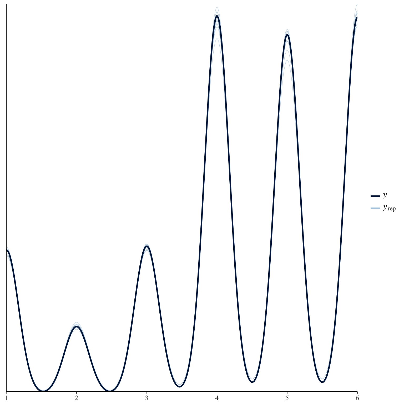
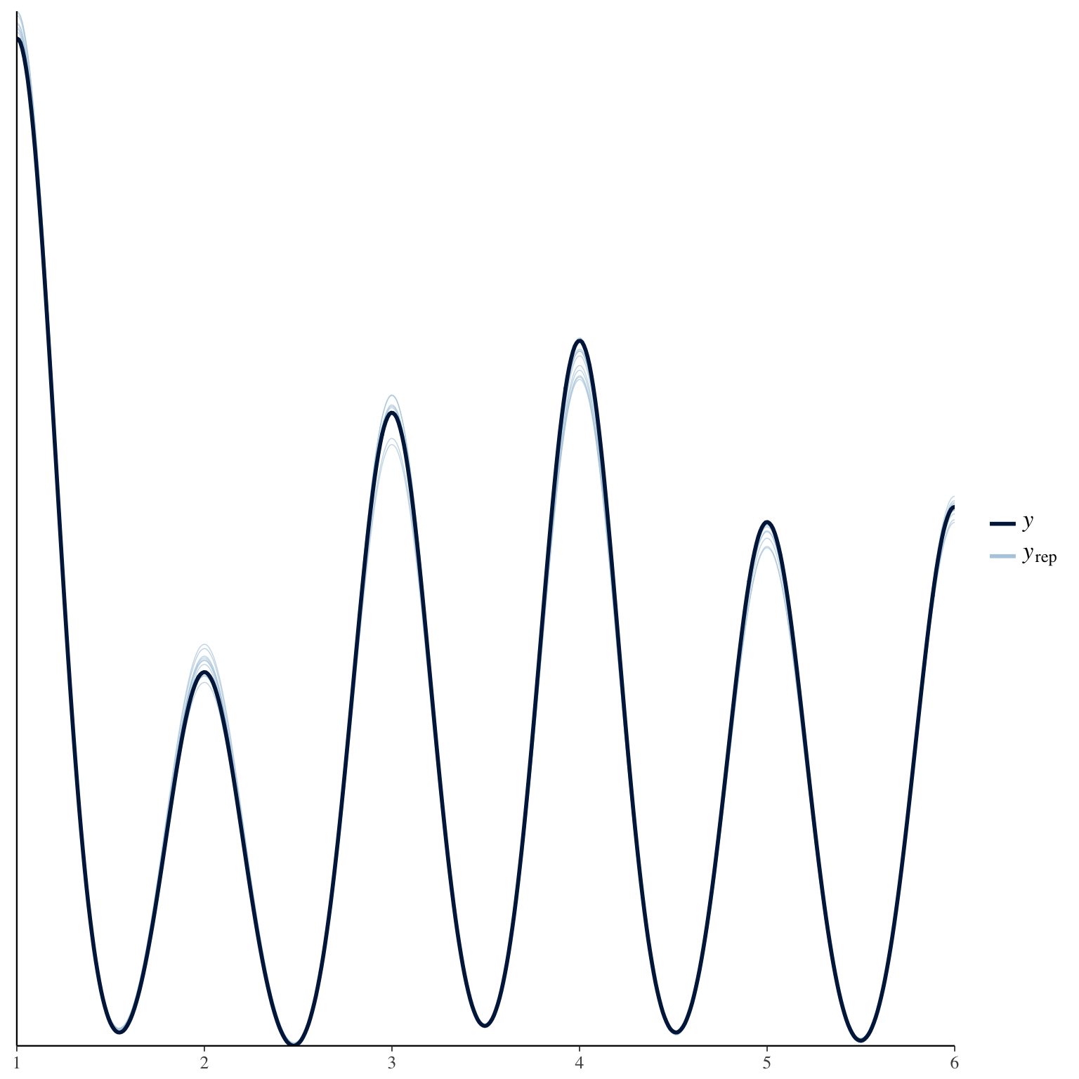
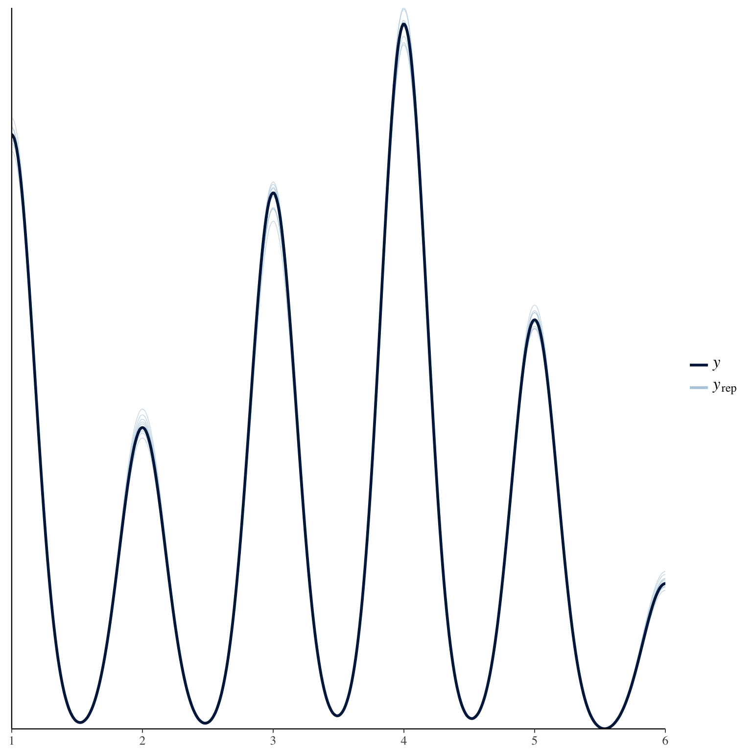
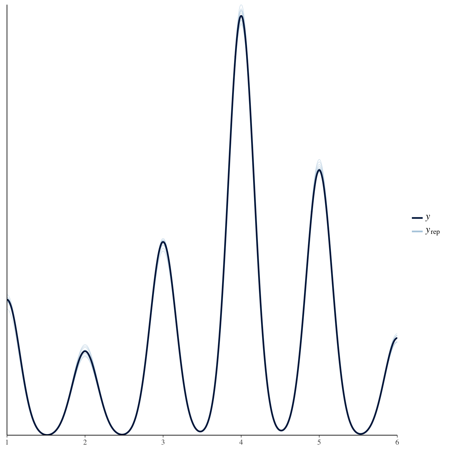
print(pp_check(fit))
}, error = function(e) warning(e))
}, error = function(e){cat_message(e, "danger")})
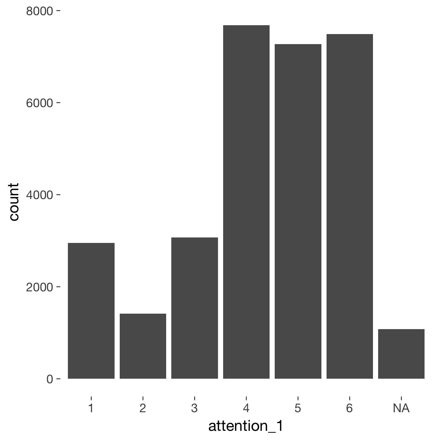
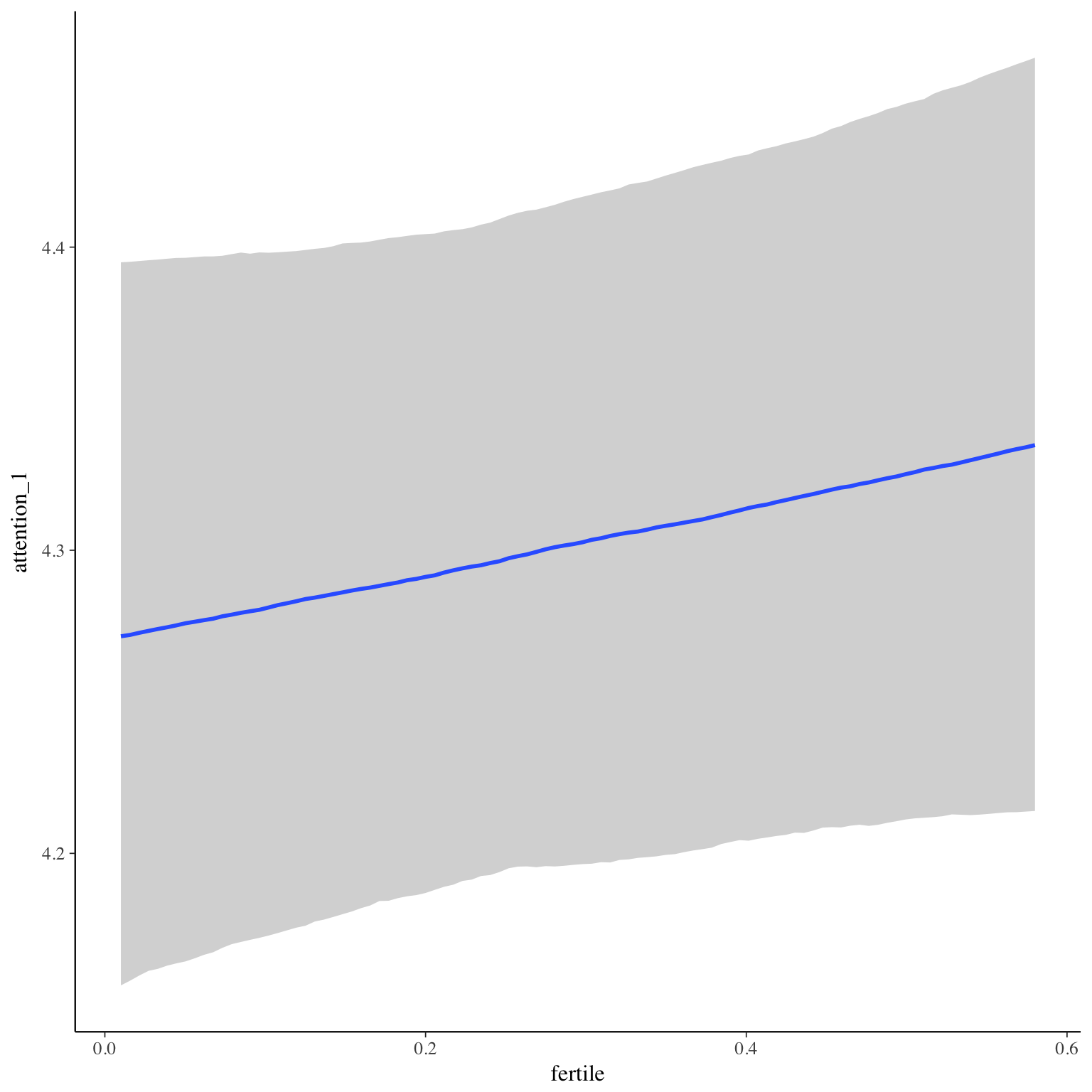
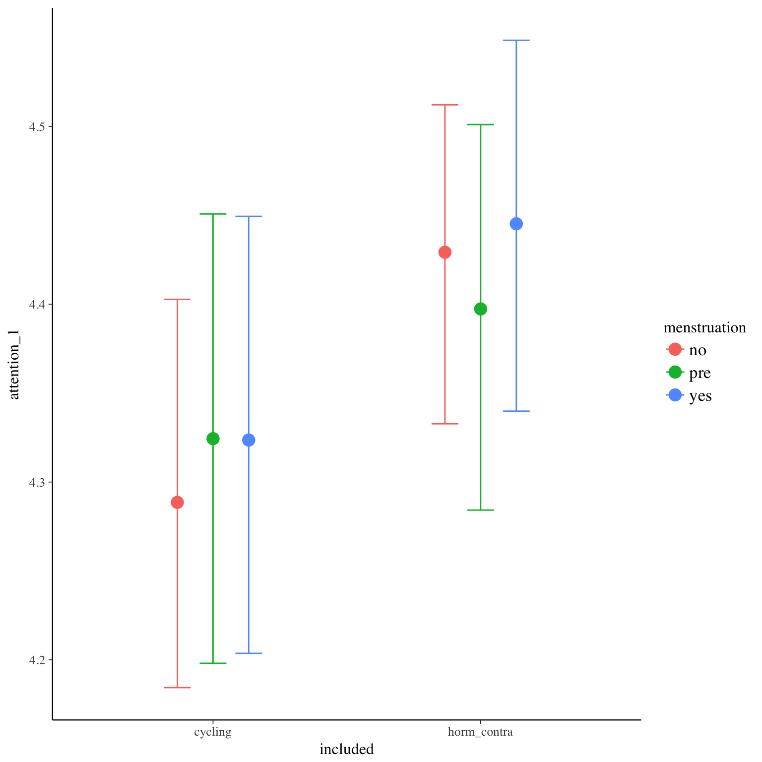
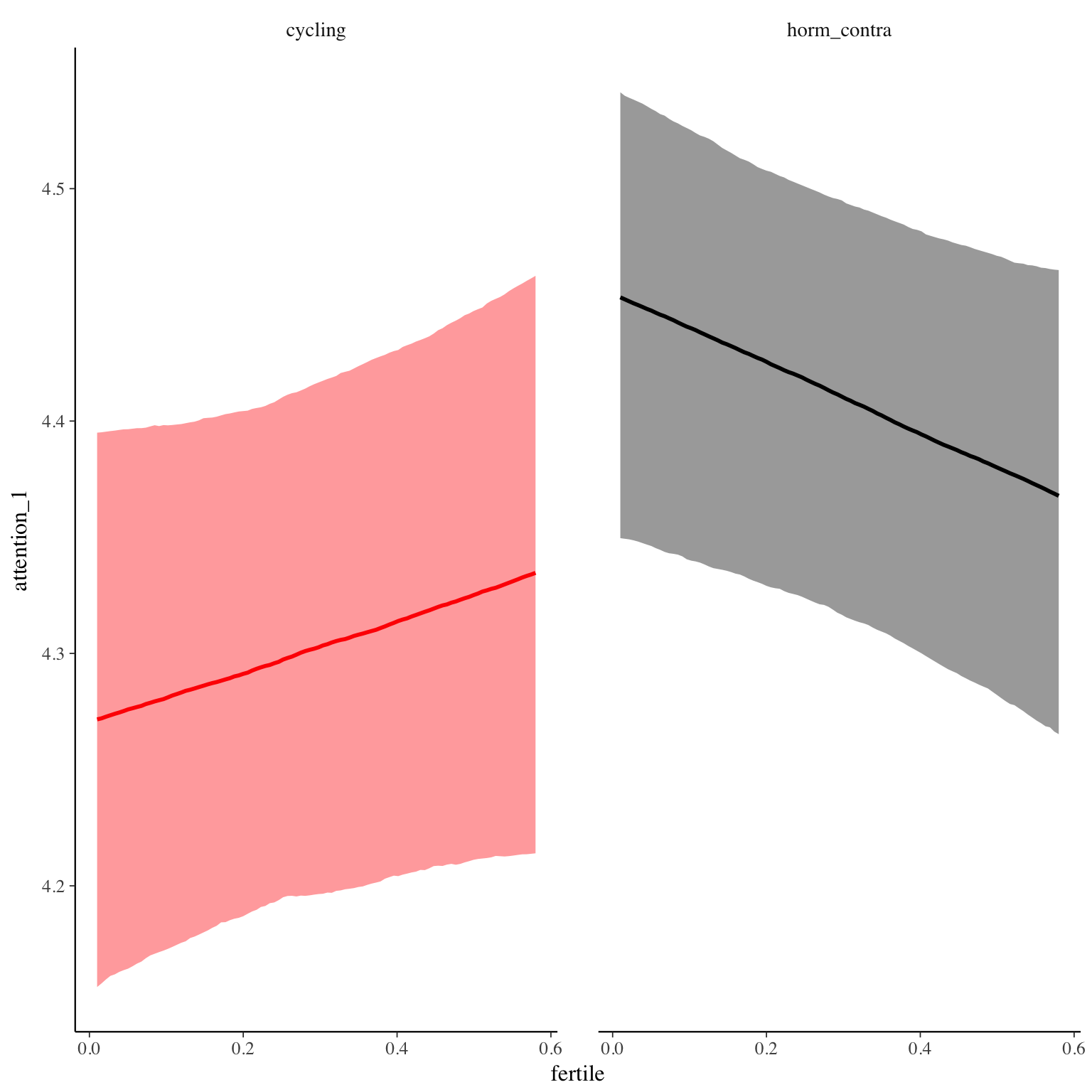
}attention_1
Item text:
… habe ich meinem Partner gezeigt, dass er mir wichtig ist.
Item translation:
41. I showed my partner that he is important to me.
Choices:
| choice | value | frequency | percent |
|---|---|---|---|
| 1 | Stimme nicht zu | 2950 | 0.1 |
| 2 | Stimme überwiegend nicht zu | 1413 | 0.05 |
| 3 | Stimme eher nicht zu | 3069 | 0.1 |
| 4 | Stimme eher zu | 7681 | 0.26 |
| 5 | Stimme überwiegend zu | 7269 | 0.24 |
| 6 | Stimme voll zu | 7492 | 0.25 |
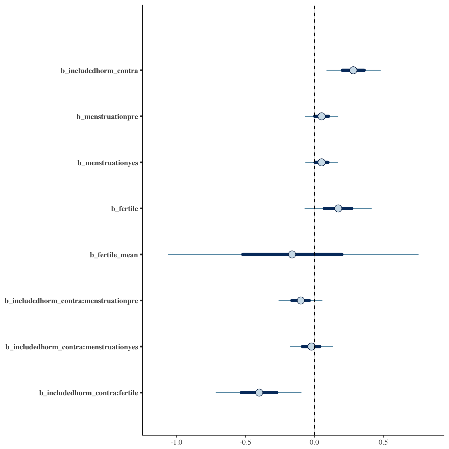
Model
Model summary
Family: cumulative(logit)
Formula: attention_1 ~ included * (menstruation + fertile) + fertile_mean + (1 + fertile + menstruation | person)
disc = 1
Data: diary (Number of observations: 26544)
Samples: 4 chains, each with iter = 2000; warmup = 1000; thin = 1;
total post-warmup samples = 4000
ICs: LOO = 74193.79; WAIC = Not computed
Group-Level Effects:
~person (Number of levels: 1043)
Estimate Est.Error l-95% CI u-95% CI Eff.Sample Rhat
sd(Intercept) 1.69 0.05 1.59 1.79 563 1.01
sd(fertile) 1.53 0.12 1.29 1.76 564 1.00
sd(menstruationpre) 0.71 0.06 0.59 0.83 614 1.00
sd(menstruationyes) 0.73 0.06 0.61 0.85 618 1.00
cor(Intercept,fertile) -0.24 0.07 -0.36 -0.10 1476 1.00
cor(Intercept,menstruationpre) -0.12 0.08 -0.26 0.04 1357 1.00
cor(fertile,menstruationpre) 0.34 0.10 0.13 0.52 443 1.00
cor(Intercept,menstruationyes) -0.17 0.07 -0.31 -0.03 1441 1.00
cor(fertile,menstruationyes) 0.39 0.09 0.19 0.56 550 1.00
cor(menstruationpre,menstruationyes) 0.54 0.09 0.35 0.70 518 1.01
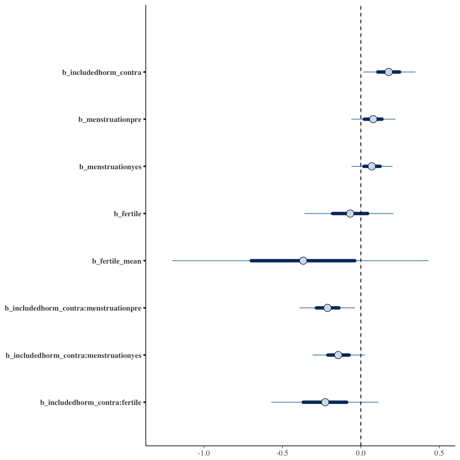
Population-Level Effects:
Estimate Est.Error l-95% CI u-95% CI Eff.Sample Rhat
Intercept[1] -2.93 0.13 -3.19 -2.67 624 1.01
Intercept[2] -2.35 0.13 -2.60 -2.10 622 1.01
Intercept[3] -1.46 0.13 -1.71 -1.21 621 1.01
Intercept[4] 0.15 0.13 -0.10 0.40 620 1.01
Intercept[5] 1.71 0.13 1.46 1.96 622 1.01
includedhorm_contra 0.28 0.12 0.04 0.51 420 1.01
menstruationpre 0.05 0.07 -0.09 0.19 1224 1.00
menstruationyes 0.05 0.07 -0.08 0.19 1190 1.00
fertile 0.17 0.15 -0.12 0.46 1293 1.00
fertile_mean -0.16 0.55 -1.24 0.90 1076 1.00
includedhorm_contra:menstruationpre -0.10 0.09 -0.28 0.08 1195 1.00
includedhorm_contra:menstruationyes -0.02 0.09 -0.20 0.16 1164 1.00
includedhorm_contra:fertile -0.40 0.19 -0.78 -0.03 1184 1.00
Samples were drawn using sampling(NUTS). For each parameter, Eff.Sample
is a crude measure of effective sample size, and Rhat is the potential
scale reduction factor on split chains (at convergence, Rhat = 1).
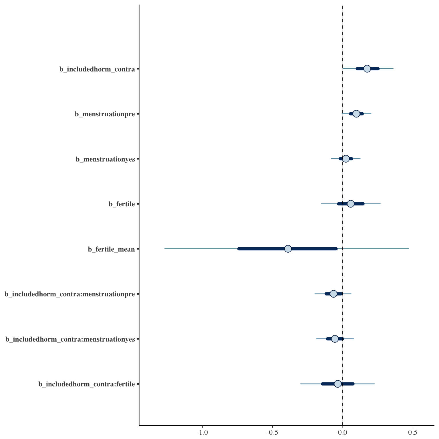
Coefficient plot
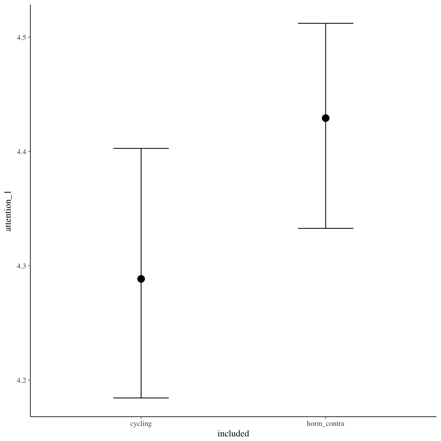
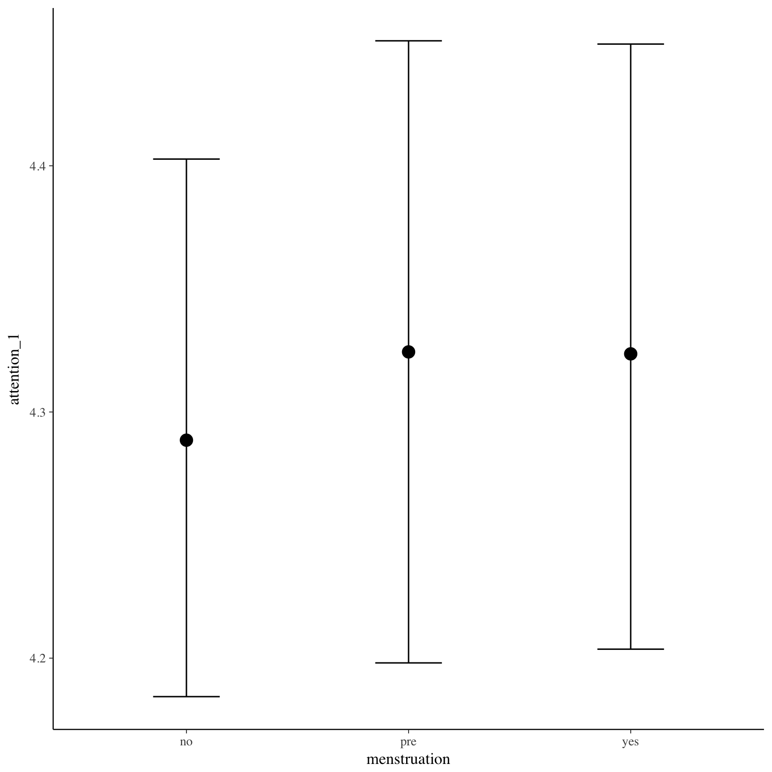
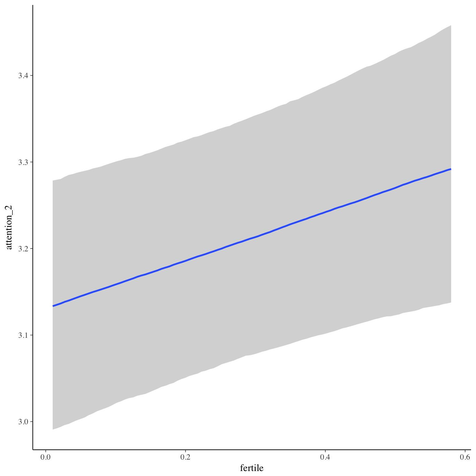
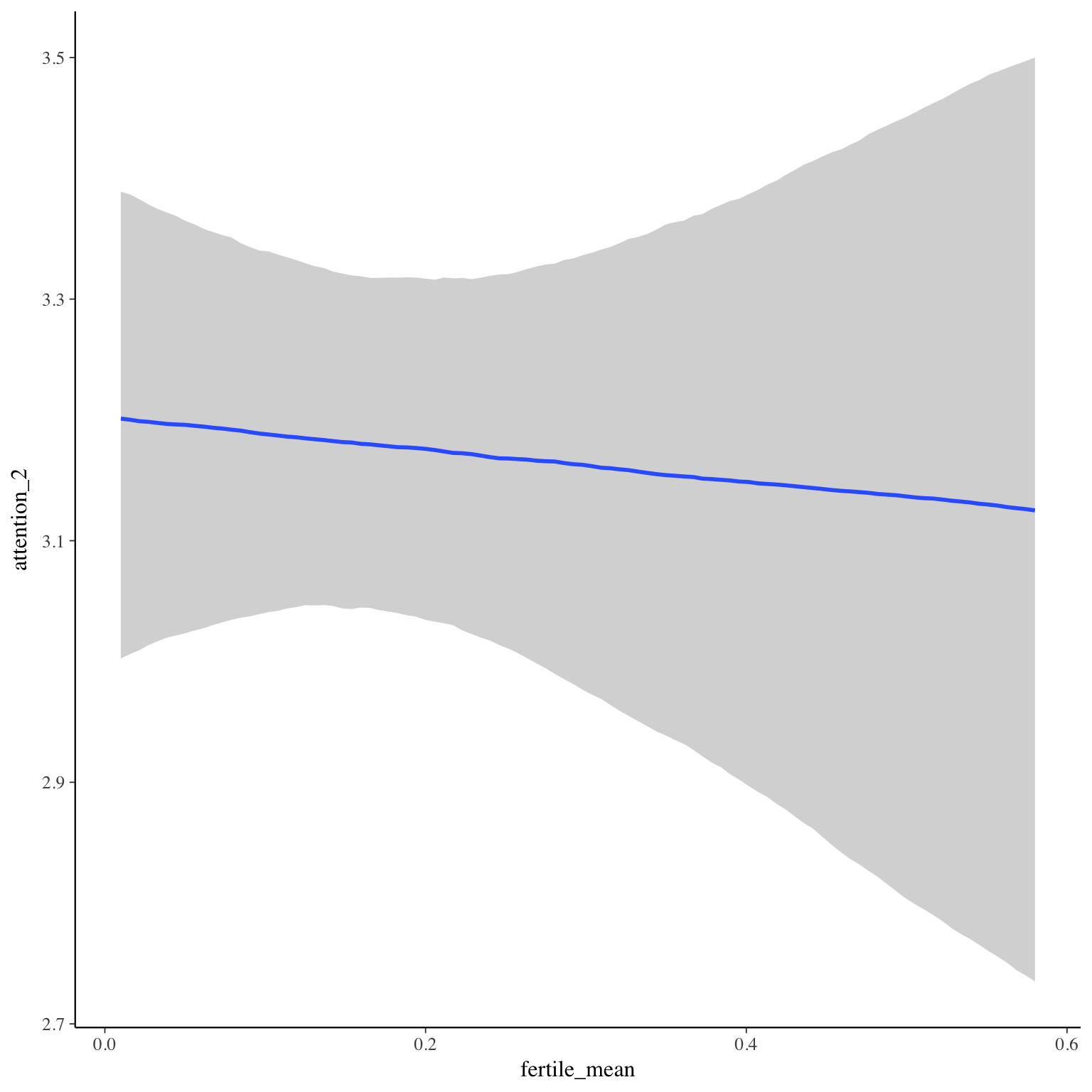
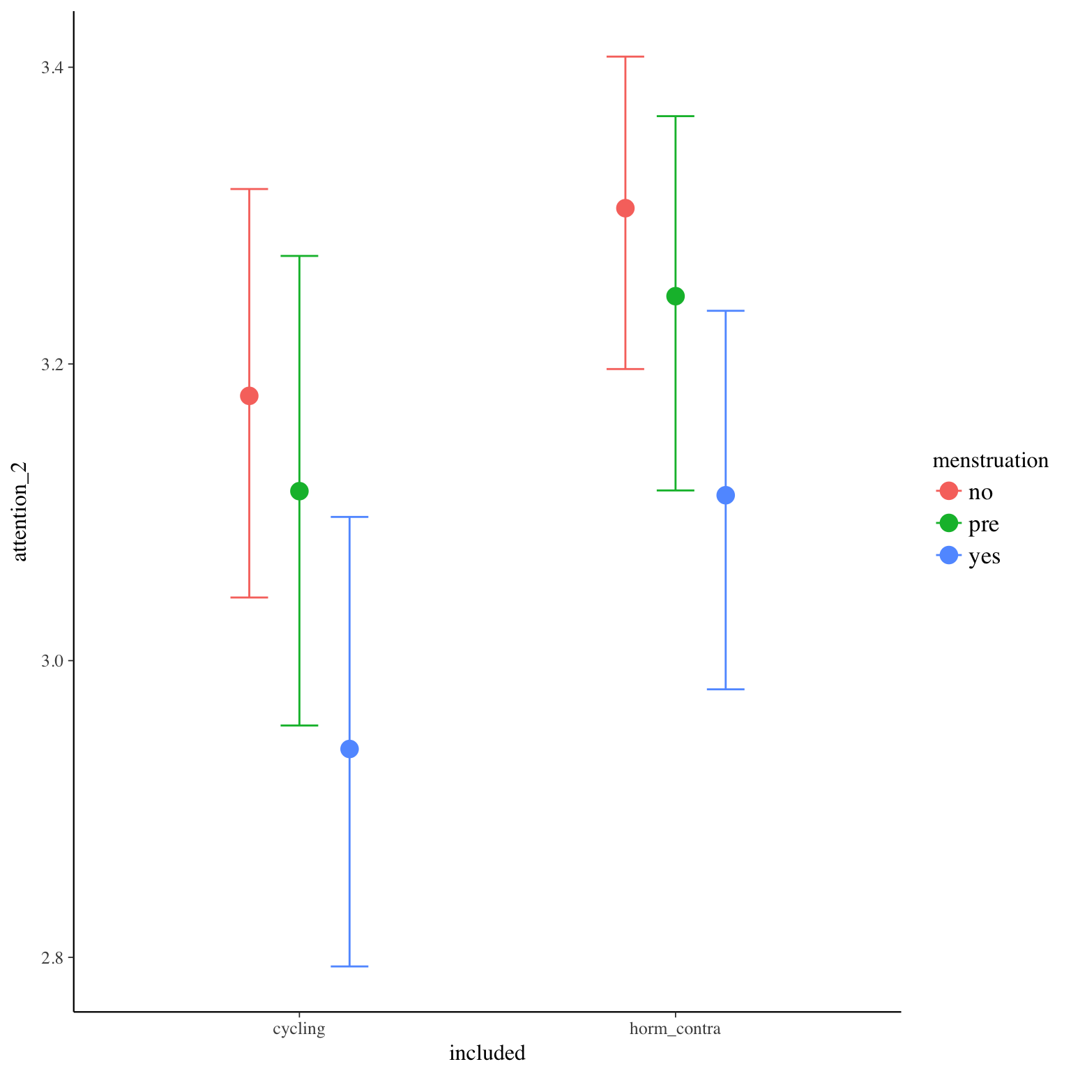
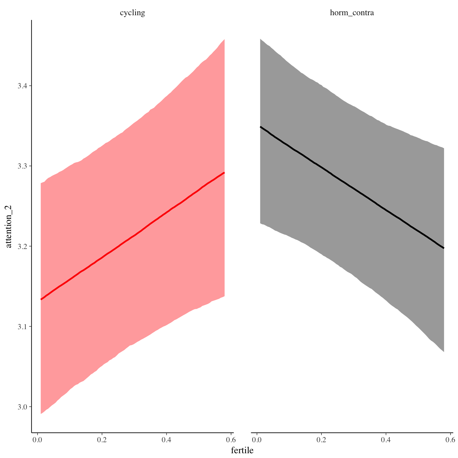
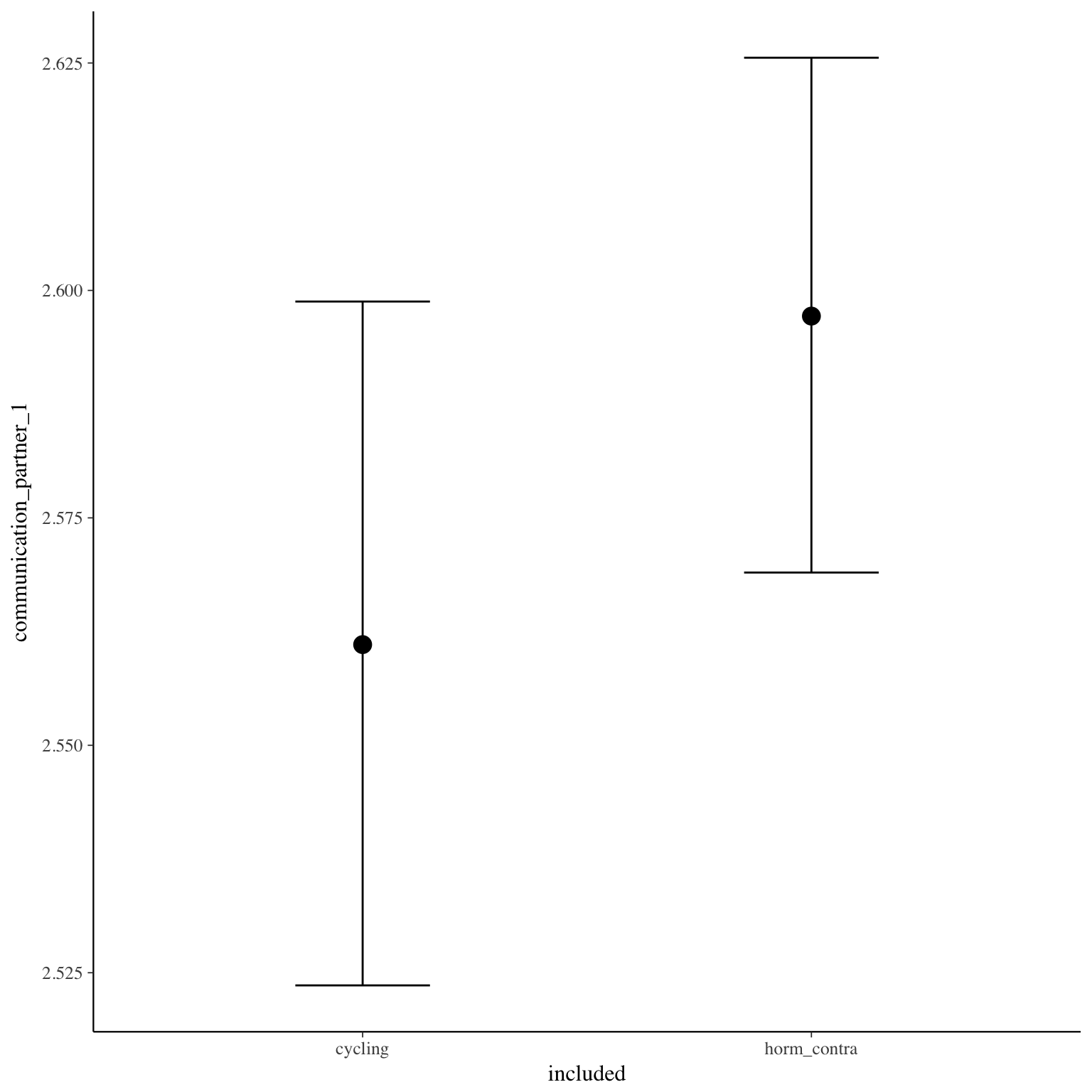
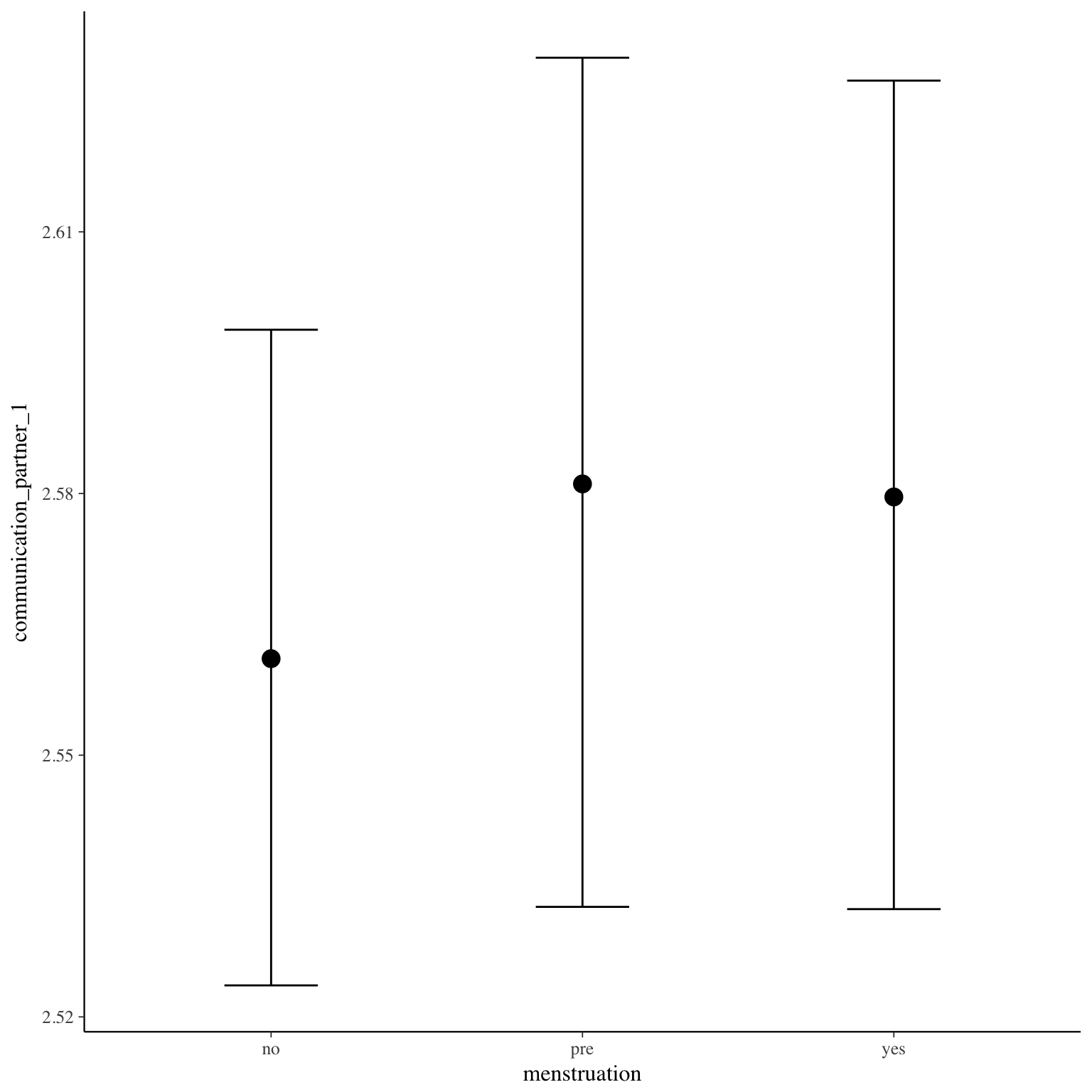
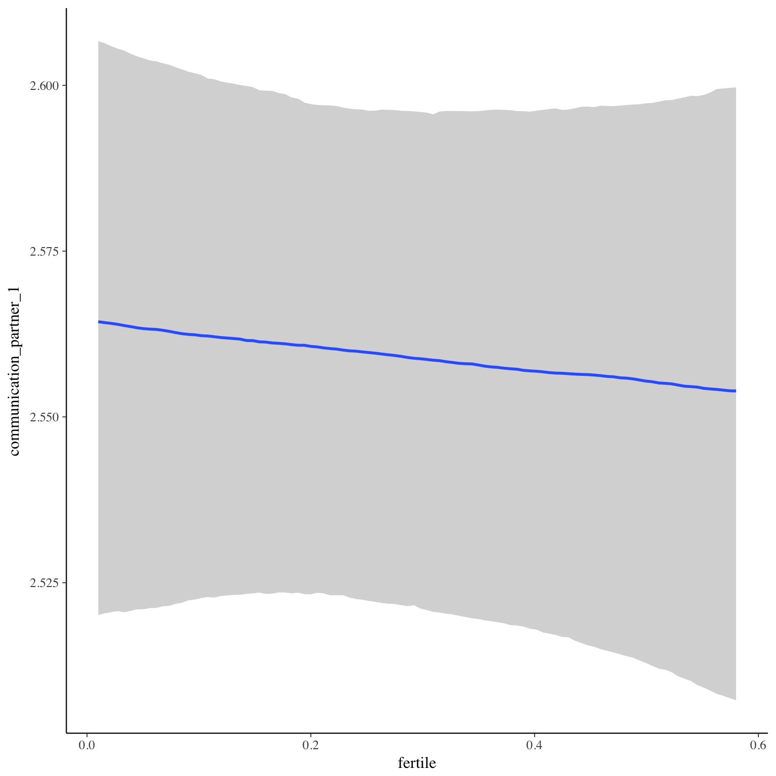
Marginal effect plots

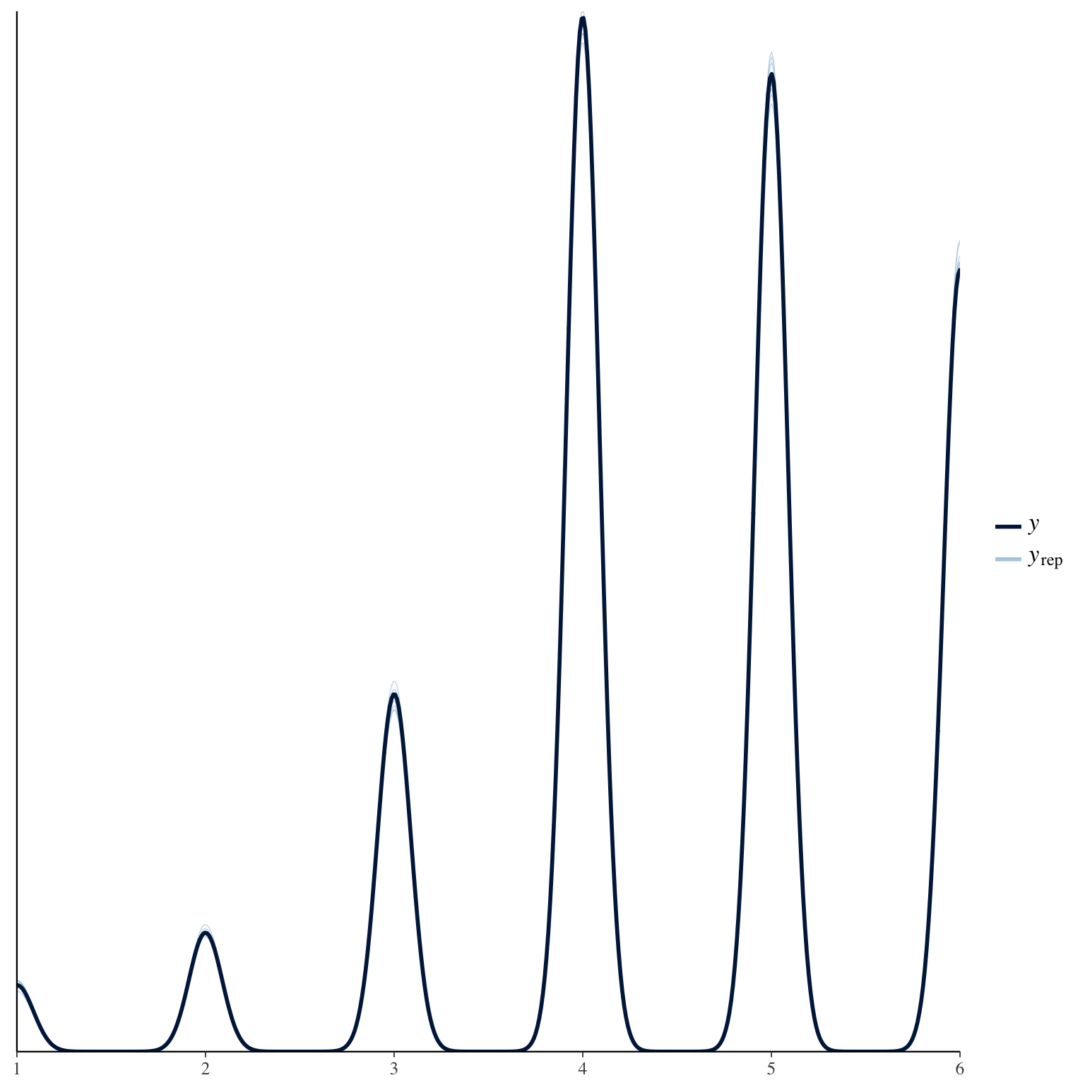
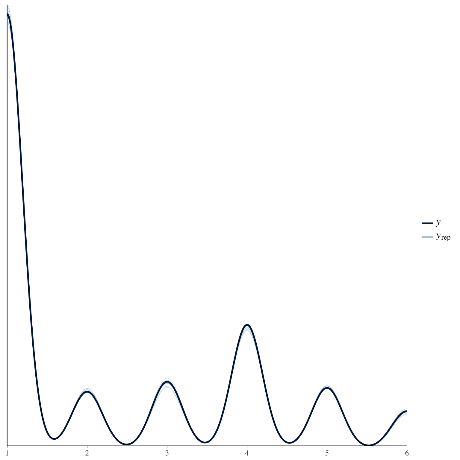
Diagnostics
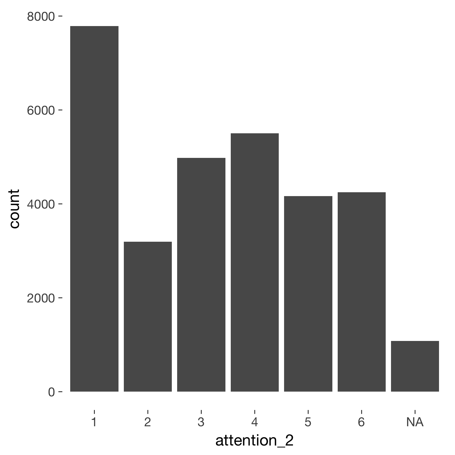
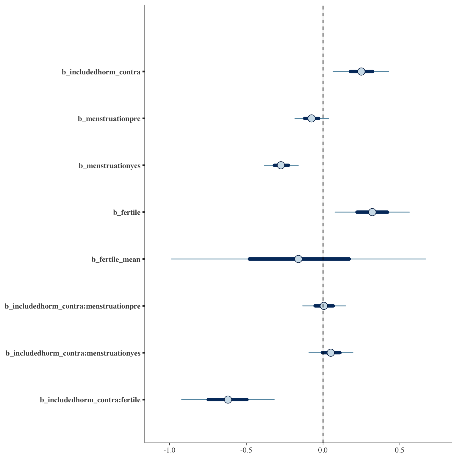
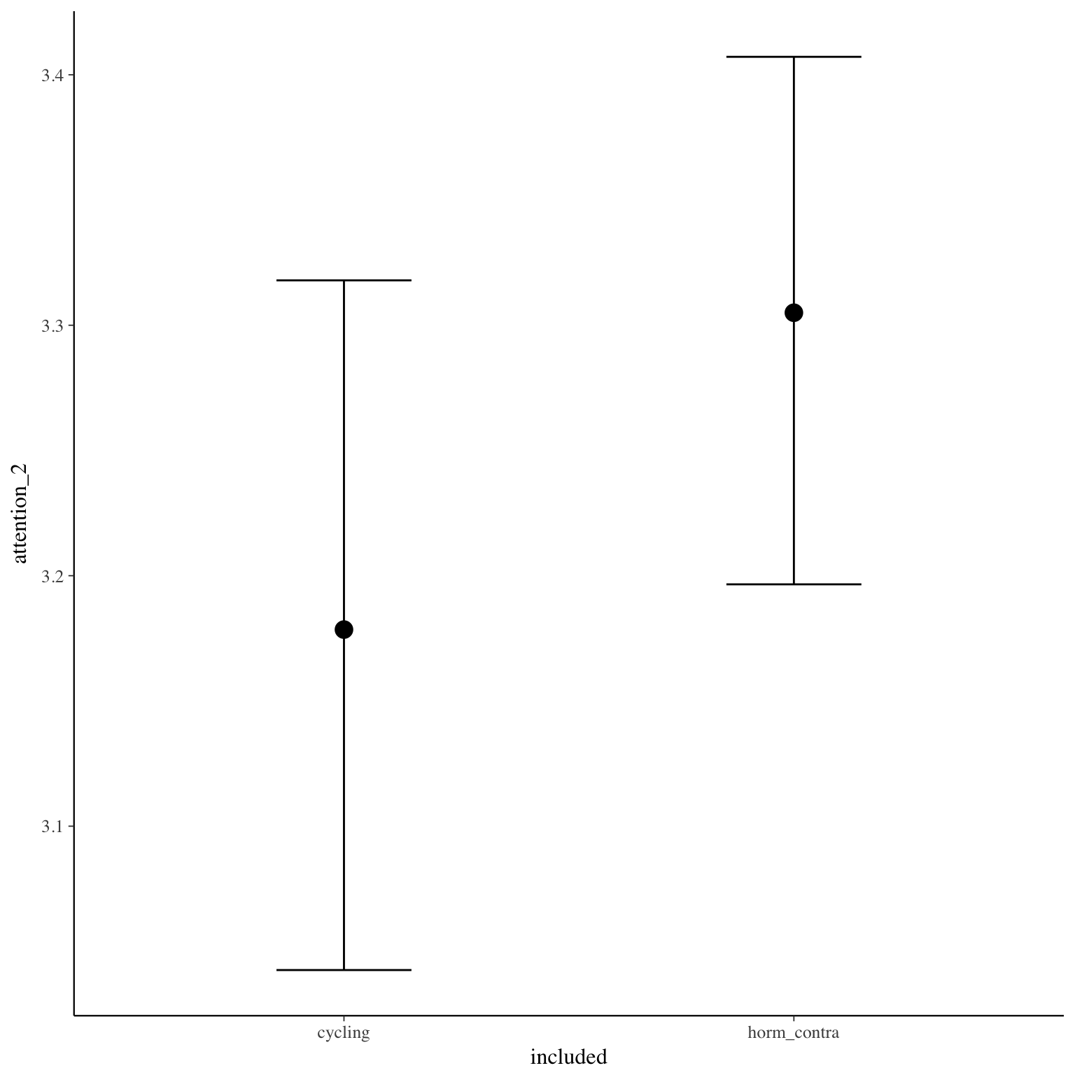
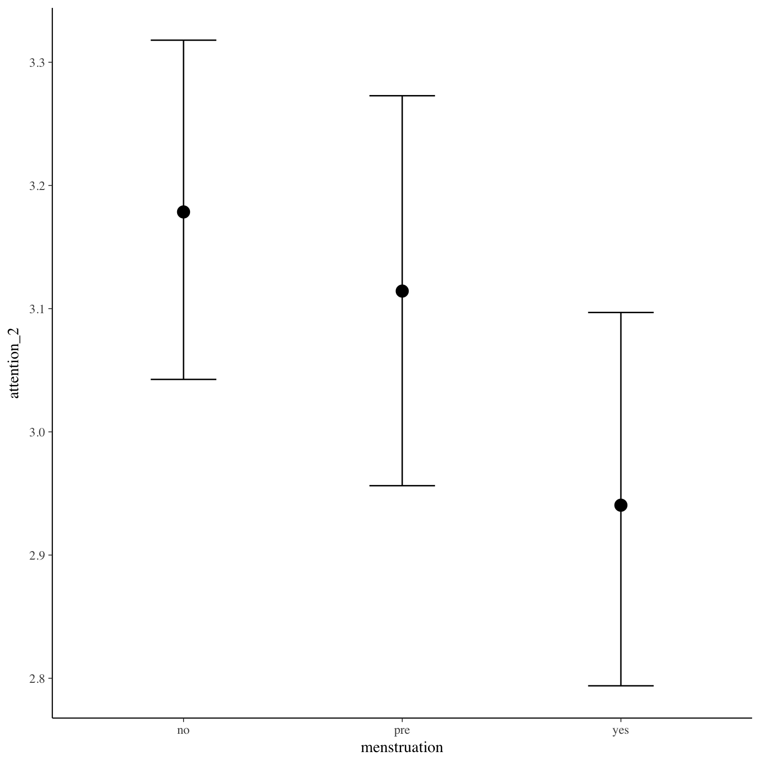
attention_2
Item text:
… habe ich meinem Partner gezeigt, dass ich mich von ihm sexuell angezogen fühle.
Item translation:
42. I showed my partner that I was sexually attracted to him.
Choices:
| choice | value | frequency | percent |
|---|---|---|---|
| 1 | Stimme nicht zu | 7785 | 0.26 |
| 2 | Stimme überwiegend nicht zu | 3194 | 0.11 |
| 3 | Stimme eher nicht zu | 4982 | 0.17 |
| 4 | Stimme eher zu | 5502 | 0.18 |
| 5 | Stimme überwiegend zu | 4166 | 0.14 |
| 6 | Stimme voll zu | 4245 | 0.14 |
Model
Model summary
 Family: cumulative(logit)
Formula: attention_2 ~ included * (menstruation + fertile) + fertile_mean + (1 + fertile + menstruation | person)
         disc = 1
   Data: diary (Number of observations: 26544)
Samples: 4 chains, each with iter = 2000; warmup = 1000; thin = 1;
         total post-warmup samples = 4000
    ICs: LOO = 83451.19; WAIC = Not computed

Group-Level Effects:
~person (Number of levels: 1043)
                                     Estimate Est.Error l-95% CI u-95% CI Eff.Sample Rhat
sd(Intercept)                            1.47      0.05     1.38     1.56       1188 1.00
sd(fertile)                              1.66      0.11     1.44     1.89        774 1.00
sd(menstruationpre)                      0.63      0.06     0.51     0.76        645 1.01
sd(menstruationyes)                      0.65      0.06     0.54     0.77        731 1.01
cor(Intercept,fertile)                  -0.27      0.06    -0.40    -0.14       1911 1.00
cor(Intercept,menstruationpre)          -0.21      0.08    -0.37    -0.05       2237 1.00
cor(fertile,menstruationpre)             0.37      0.10     0.17     0.55        718 1.01
cor(Intercept,menstruationyes)          -0.22      0.08    -0.37    -0.07       2266 1.00
cor(fertile,menstruationyes)             0.25      0.10     0.06     0.43        559 1.01
cor(menstruationpre,menstruationyes)     0.31      0.12     0.06     0.52        480 1.01

Population-Level Effects:
                                    Estimate Est.Error l-95% CI u-95% CI Eff.Sample Rhat
Intercept[1]                           -1.30      0.12    -1.53    -1.06        773 1.00
Intercept[2]                           -0.62      0.12    -0.85    -0.39        769 1.00
Intercept[3]                            0.29      0.12     0.07     0.53        773 1.00
Intercept[4]                            1.33      0.12     1.11     1.58        780 1.00
Intercept[5]                            2.41      0.12     2.18     2.66        788 1.00
includedhorm_contra                     0.25      0.11     0.03     0.46        604 1.01
menstruationpre                        -0.07      0.07    -0.21     0.06       2105 1.00
menstruationyes                        -0.27      0.07    -0.40    -0.14       1932 1.00
fertile                                 0.32      0.15     0.03     0.60       1667 1.00
fertile_mean                           -0.16      0.50    -1.18     0.84       1211 1.00
includedhorm_contra:menstruationpre     0.01      0.09    -0.15     0.17       2172 1.00
includedhorm_contra:menstruationyes     0.05      0.09    -0.12     0.22       2014 1.00
includedhorm_contra:fertile            -0.62      0.19    -0.98    -0.27       1486 1.00

Samples were drawn using sampling(NUTS). For each parameter, Eff.Sample
is a crude measure of effective sample size, and Rhat is the potential
scale reduction factor on split chains (at convergence, Rhat = 1).
Coefficient plot
Marginal effect plots
Diagnostics
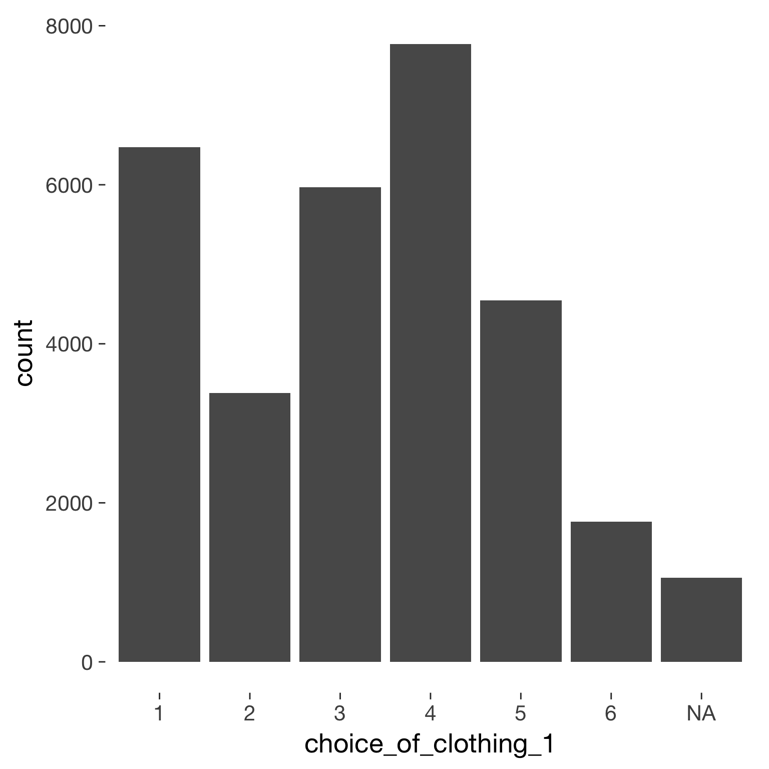
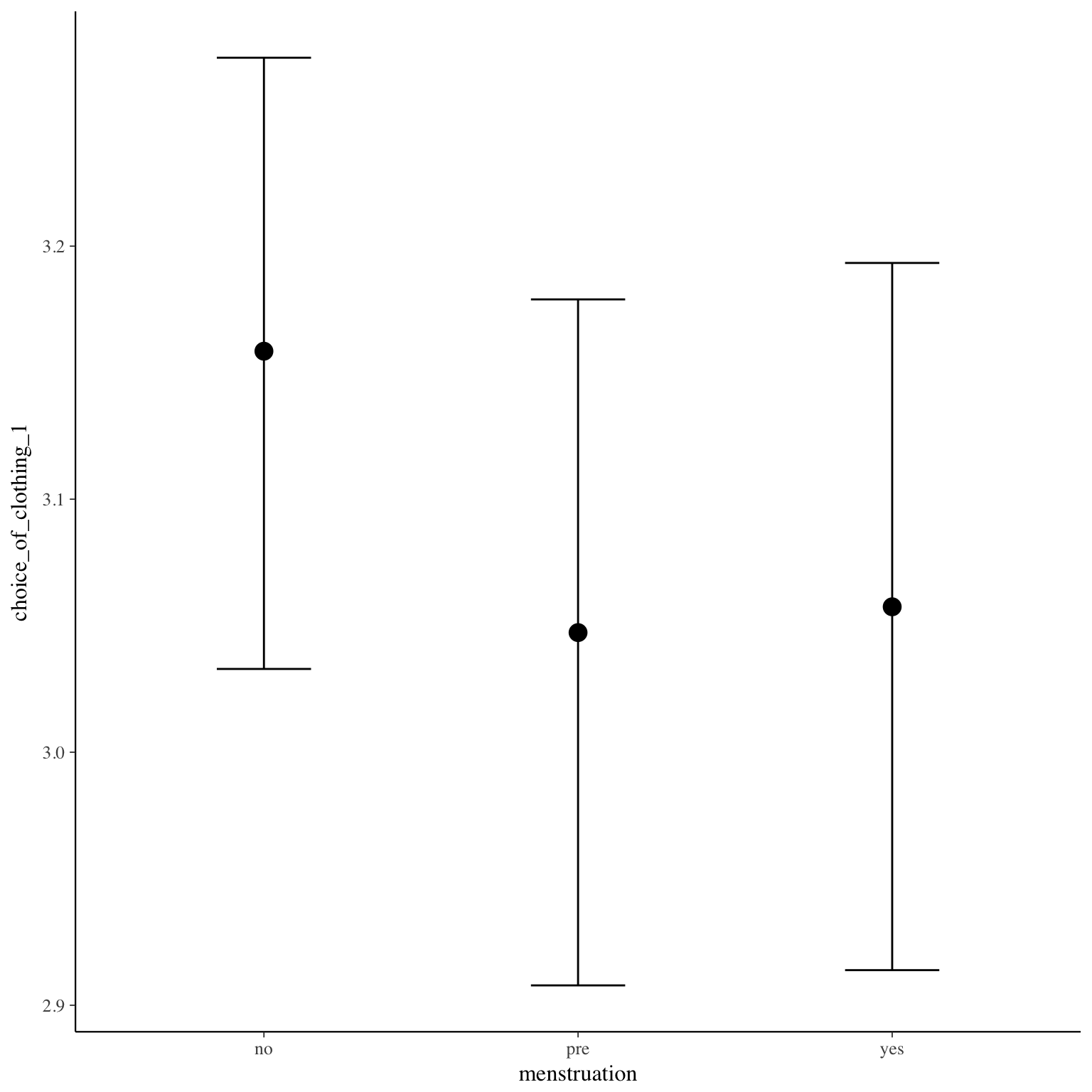
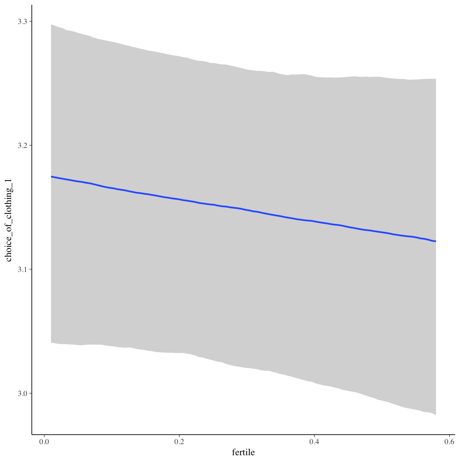
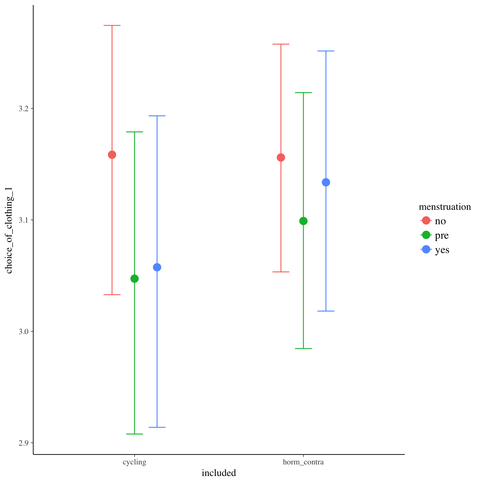
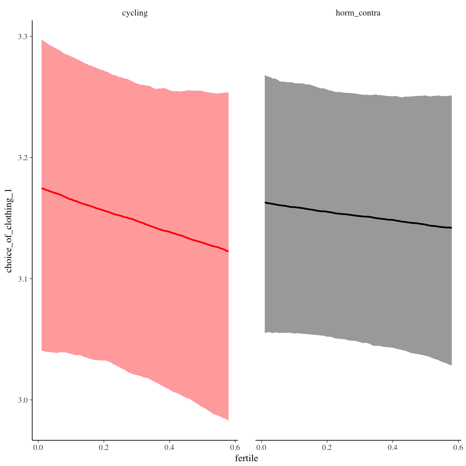
choice_of_clothing_1
Item text:
Seriös
Item translation:
16. respectable
Choices:
| choice | value | frequency | percent |
|---|---|---|---|
| 1 | Stimme nicht zu | 6472 | 0.22 |
| 2 | Stimme überwiegend nicht zu | 3381 | 0.11 |
| 3 | Stimme eher nicht zu | 5966 | 0.2 |
| 4 | Stimme eher zu | 7768 | 0.26 |
| 5 | Stimme überwiegend zu | 4545 | 0.15 |
| 6 | Stimme voll zu | 1764 | 0.06 |
Model
Model summary
Family: cumulative(logit)
Formula: choice_of_clothing_1 ~ included * (menstruation + fertile) + fertile_mean + (1 + fertile + menstruation | person)
disc = 1
Data: diary (Number of observations: 26562)
Samples: 4 chains, each with iter = 2000; warmup = 1000; thin = 1;
total post-warmup samples = 4000
ICs: LOO = 77486.23; WAIC = Not computed
Group-Level Effects:
~person (Number of levels: 1043)
Estimate Est.Error l-95% CI u-95% CI Eff.Sample Rhat
sd(Intercept) 1.67 0.05 1.57 1.77 362 1.00
sd(fertile) 1.10 0.12 0.86 1.35 278 1.01
sd(menstruationpre) 0.20 0.13 0.01 0.46 86 1.04
sd(menstruationyes) 0.51 0.07 0.37 0.63 341 1.00
cor(Intercept,fertile) -0.22 0.08 -0.38 -0.04 710 1.00
cor(Intercept,menstruationpre) -0.13 0.29 -0.72 0.58 1408 1.00
cor(fertile,menstruationpre) 0.10 0.36 -0.70 0.74 370 1.01
cor(Intercept,menstruationyes) -0.01 0.10 -0.19 0.19 1589 1.00
cor(fertile,menstruationyes) 0.20 0.16 -0.12 0.48 309 1.01
cor(menstruationpre,menstruationyes) 0.21 0.36 -0.68 0.81 62 1.06
Population-Level Effects:
Estimate Est.Error l-95% CI u-95% CI Eff.Sample Rhat
Intercept[1] -1.87 0.13 -2.14 -1.62 516 1.01
Intercept[2] -1.04 0.13 -1.31 -0.79 513 1.01
Intercept[3] 0.13 0.13 -0.13 0.38 515 1.01
Intercept[4] 1.78 0.13 1.52 2.03 515 1.01
Intercept[5] 3.66 0.13 3.39 3.92 533 1.01
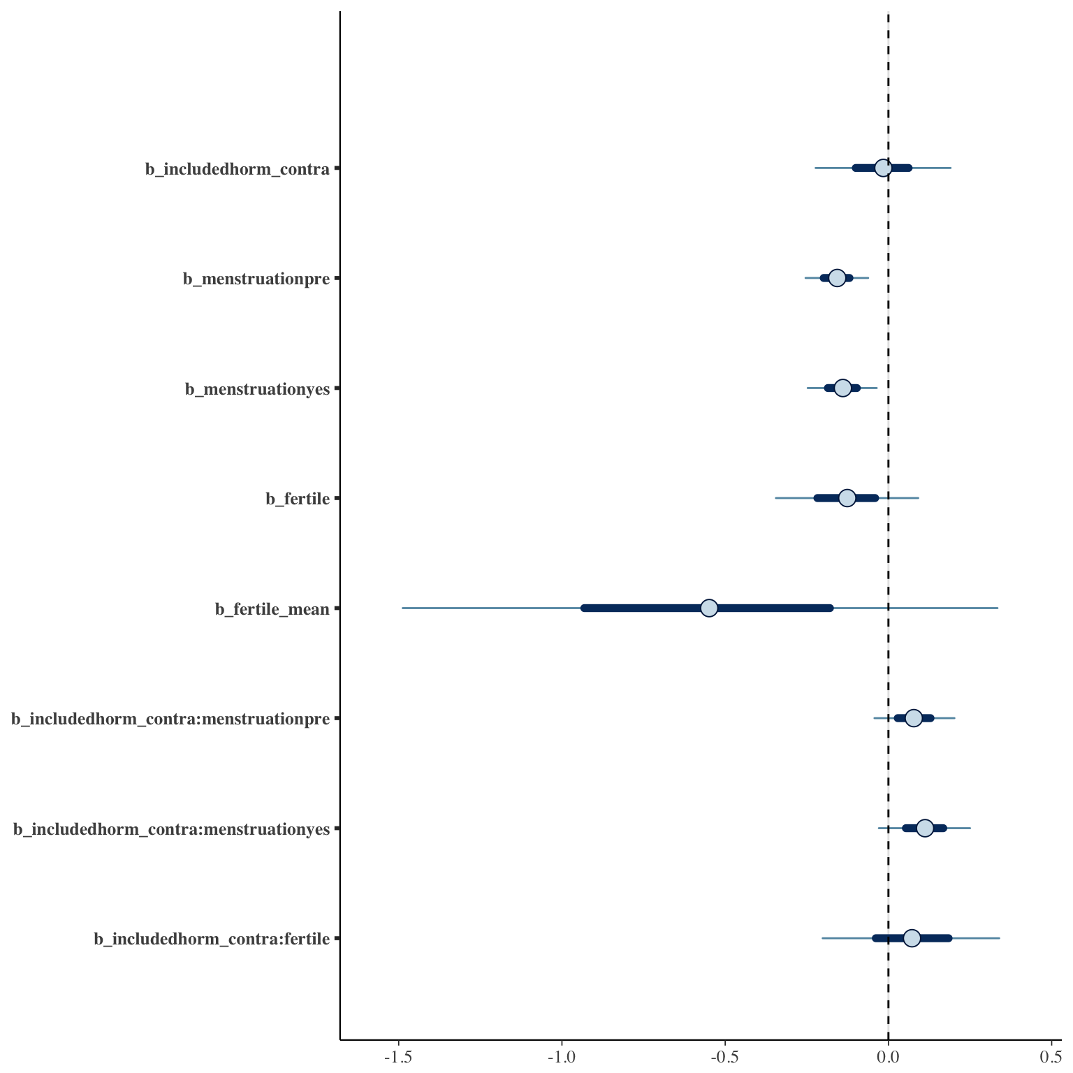
includedhorm_contra -0.02 0.12 -0.26 0.23 328 1.01
menstruationpre -0.16 0.06 -0.27 -0.05 1764 1.00
menstruationyes -0.14 0.06 -0.27 -0.02 1604 1.00
fertile -0.13 0.13 -0.38 0.14 1381 1.00
fertile_mean -0.56 0.56 -1.65 0.48 946 1.00
includedhorm_contra:menstruationpre 0.08 0.07 -0.07 0.23 1167 1.00
includedhorm_contra:menstruationyes 0.11 0.08 -0.05 0.27 809 1.00
includedhorm_contra:fertile 0.07 0.17 -0.26 0.41 1140 1.00
Samples were drawn using sampling(NUTS). For each parameter, Eff.Sample
is a crude measure of effective sample size, and Rhat is the potential
scale reduction factor on split chains (at convergence, Rhat = 1).
Coefficient plot
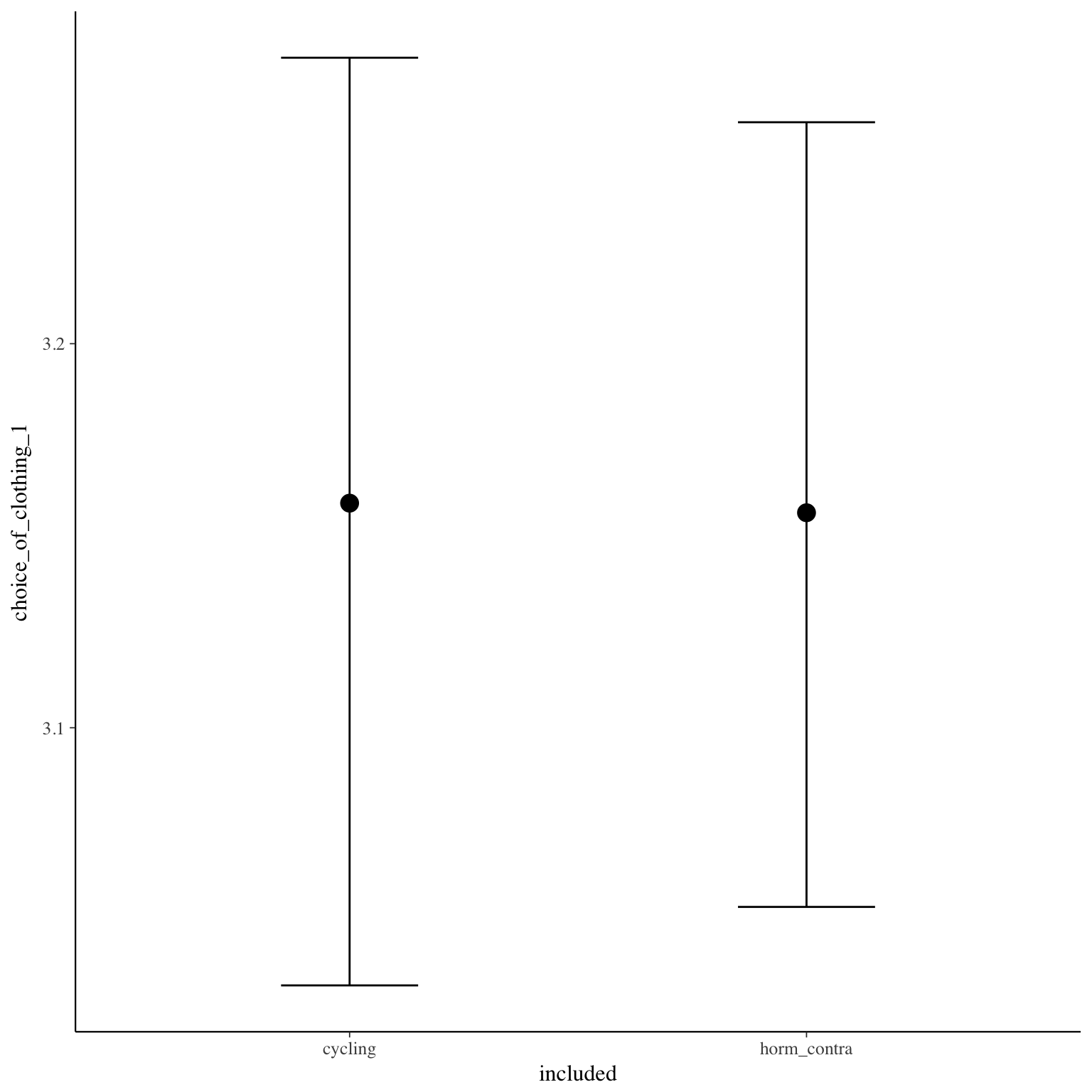
Marginal effect plots

Diagnostics
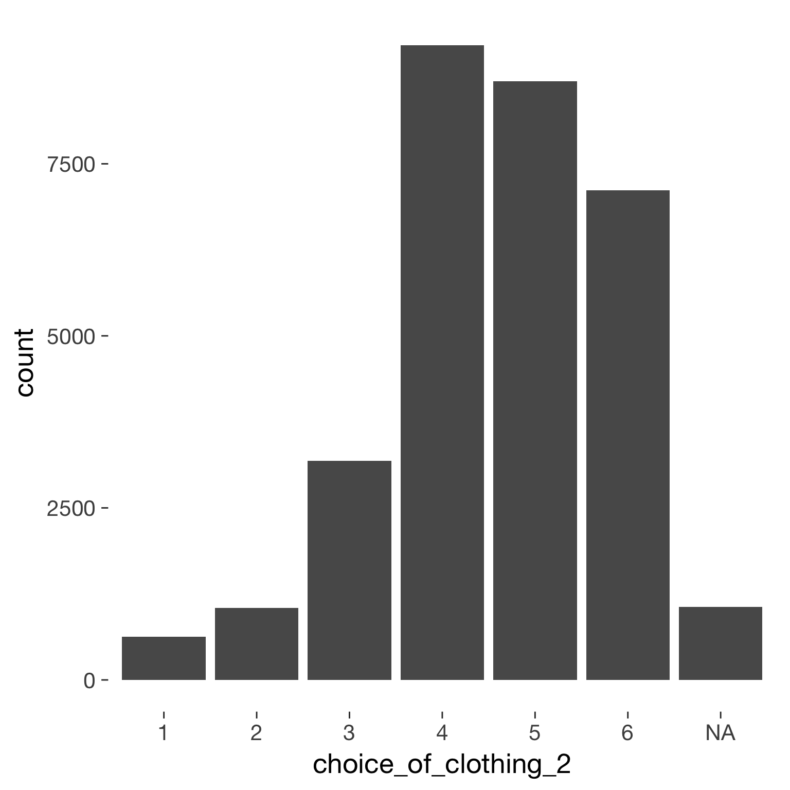
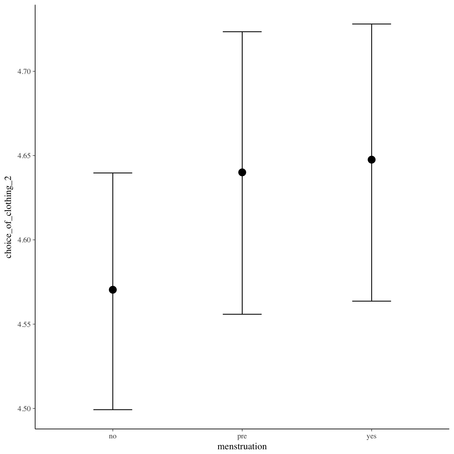
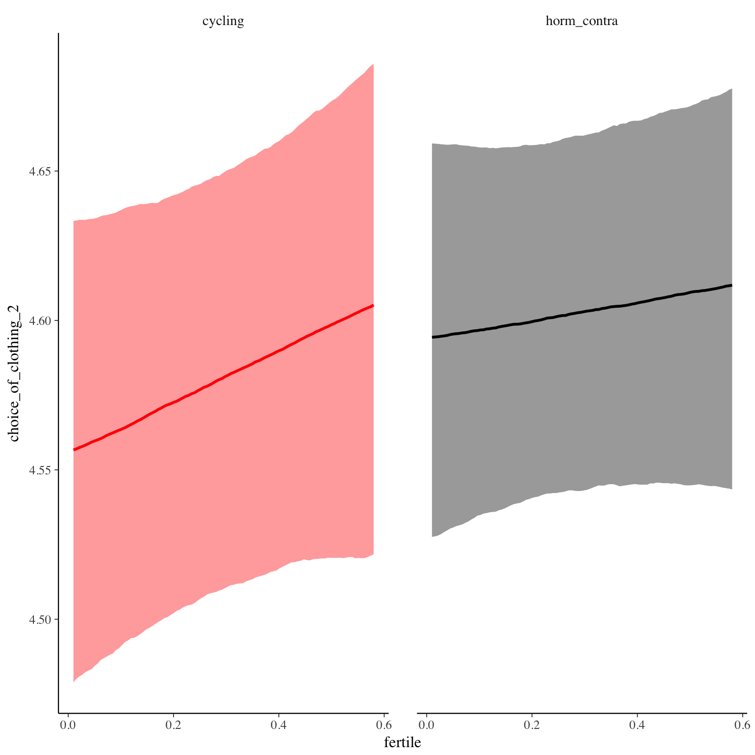
choice_of_clothing_2
Item text:
Praktisch
Item translation:
17. practical
Choices:
| choice | value | frequency | percent |
|---|---|---|---|
| 1 | Stimme nicht zu | 628 | 0.02 |
| 2 | Stimme überwiegend nicht zu | 1046 | 0.03 |
| 3 | Stimme eher nicht zu | 3185 | 0.11 |
| 4 | Stimme eher zu | 9221 | 0.31 |
| 5 | Stimme überwiegend zu | 8696 | 0.29 |
| 6 | Stimme voll zu | 7116 | 0.24 |
Model
Model summary
Family: cumulative(logit)
Formula: choice_of_clothing_2 ~ included * (menstruation + fertile) + fertile_mean + (1 + fertile + menstruation | person)
disc = 1
Data: diary (Number of observations: 26558)
Samples: 4 chains, each with iter = 2000; warmup = 1000; thin = 1;
total post-warmup samples = 4000
ICs: LOO = 72212.25; WAIC = Not computed
Group-Level Effects:
~person (Number of levels: 1043)
Estimate Est.Error l-95% CI u-95% CI Eff.Sample Rhat
sd(Intercept) 1.23 0.04 1.16 1.31 1105 1.00
sd(fertile) 1.14 0.14 0.85 1.40 390 1.01
sd(menstruationpre) 0.45 0.08 0.27 0.60 295 1.01
sd(menstruationyes) 0.28 0.11 0.03 0.46 217 1.01
cor(Intercept,fertile) -0.28 0.08 -0.43 -0.12 4000 1.00
cor(Intercept,menstruationpre) -0.17 0.10 -0.35 0.05 4000 1.00
cor(fertile,menstruationpre) 0.17 0.21 -0.30 0.48 236 1.01
cor(Intercept,menstruationyes) 0.02 0.21 -0.32 0.55 955 1.00
cor(fertile,menstruationyes) 0.36 0.28 -0.40 0.79 547 1.01
cor(menstruationpre,menstruationyes) 0.51 0.30 -0.30 0.90 391 1.01
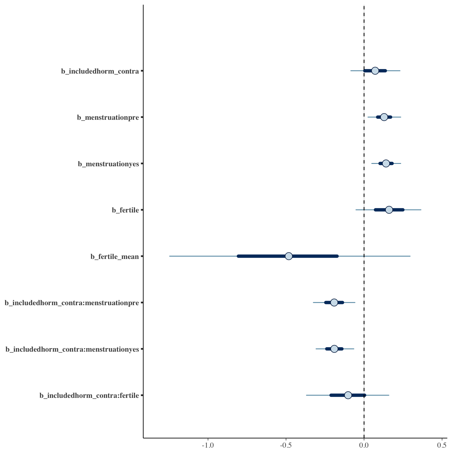
Population-Level Effects:
Estimate Est.Error l-95% CI u-95% CI Eff.Sample Rhat
Intercept[1] -4.61 0.12 -4.85 -4.39 1749 1
Intercept[2] -3.46 0.11 -3.67 -3.24 1589 1
Intercept[3] -2.09 0.11 -2.30 -1.88 1570 1
Intercept[4] -0.22 0.11 -0.43 -0.01 1577 1
Intercept[5] 1.41 0.11 1.20 1.62 1583 1
includedhorm_contra 0.07 0.10 -0.12 0.26 1100 1
menstruationpre 0.13 0.06 0.01 0.25 4000 1
menstruationyes 0.14 0.06 0.03 0.25 4000 1
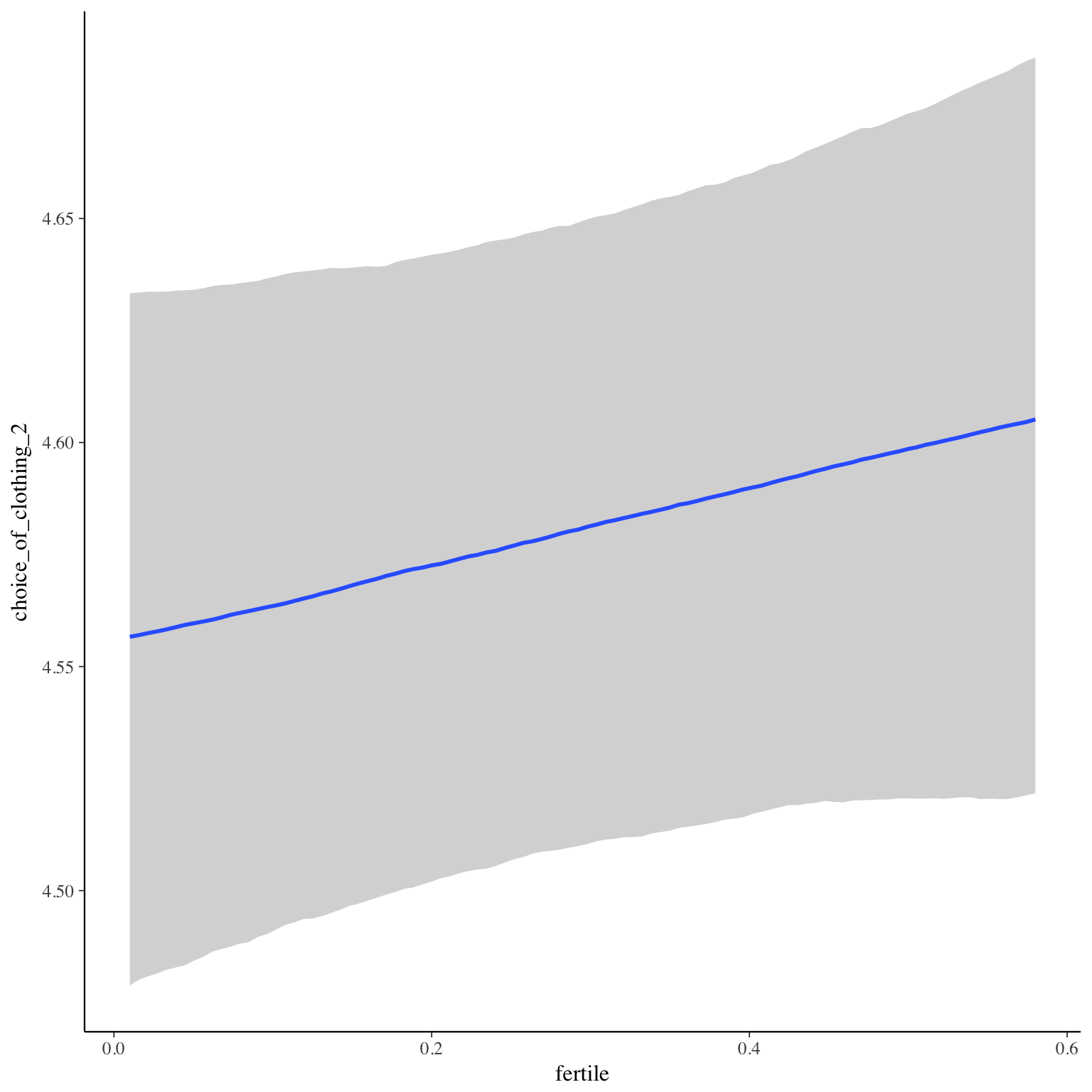
fertile 0.16 0.13 -0.09 0.41 4000 1
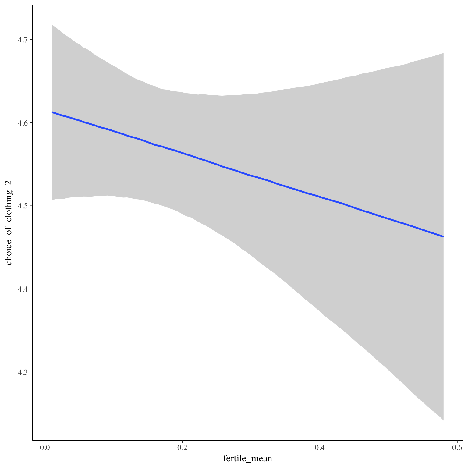
fertile_mean -0.48 0.47 -1.39 0.44 2384 1
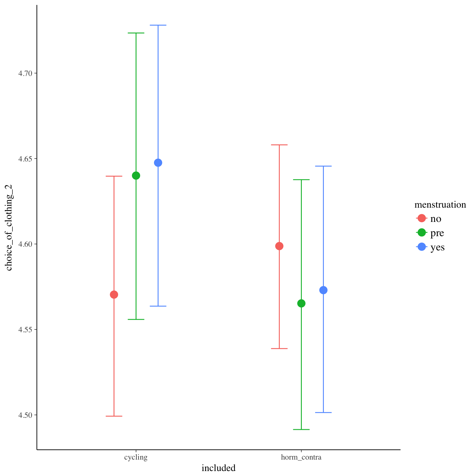
includedhorm_contra:menstruationpre -0.19 0.08 -0.35 -0.03 4000 1
includedhorm_contra:menstruationyes -0.19 0.07 -0.33 -0.04 4000 1
includedhorm_contra:fertile -0.10 0.16 -0.42 0.21 3177 1
Samples were drawn using sampling(NUTS). For each parameter, Eff.Sample
is a crude measure of effective sample size, and Rhat is the potential
scale reduction factor on split chains (at convergence, Rhat = 1).
Coefficient plot
Marginal effect plots
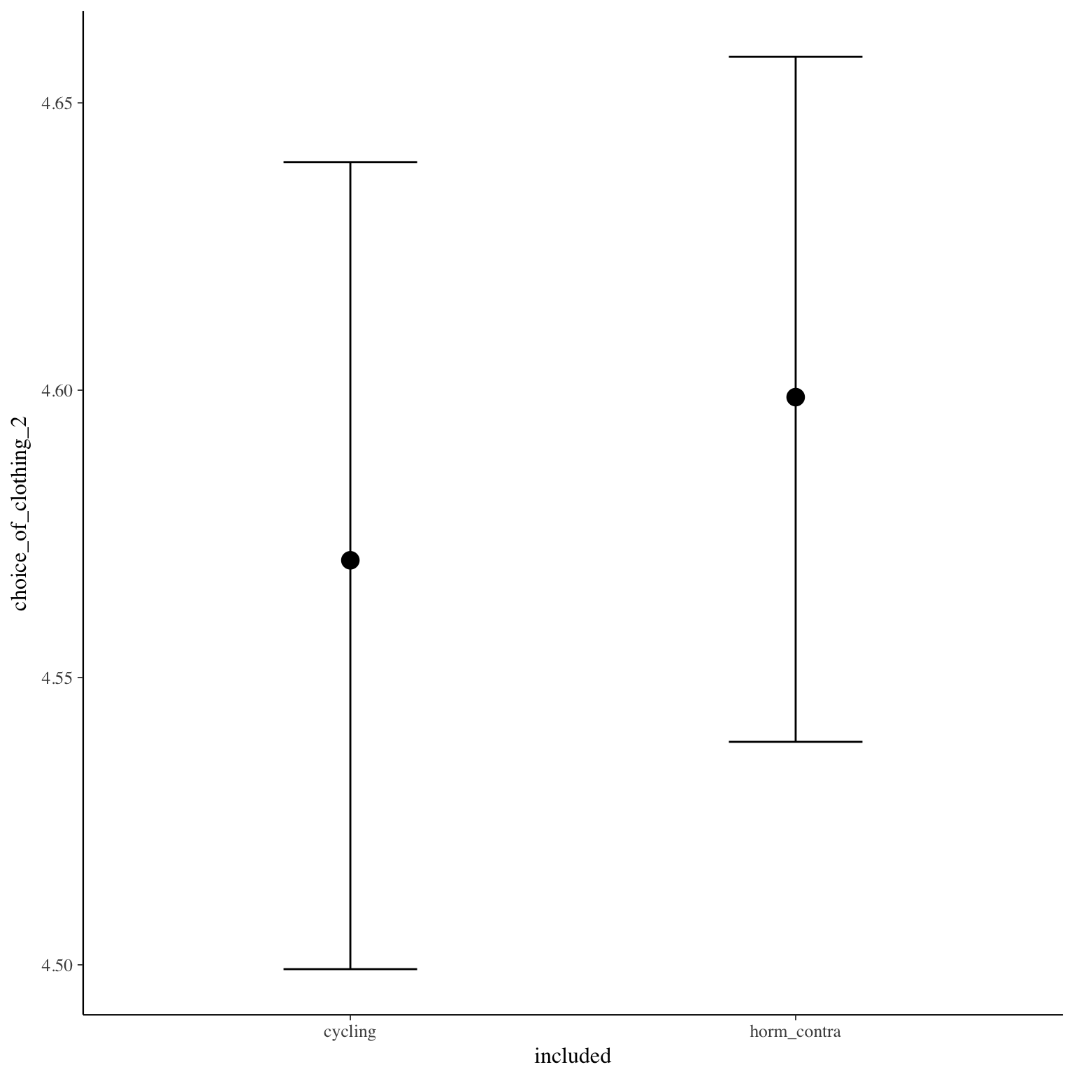
Diagnostics
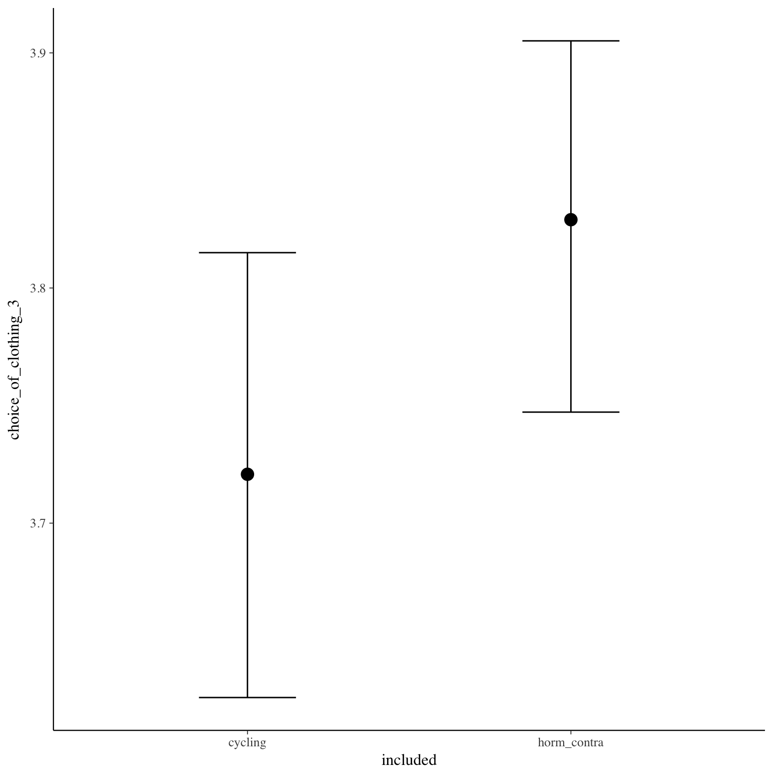
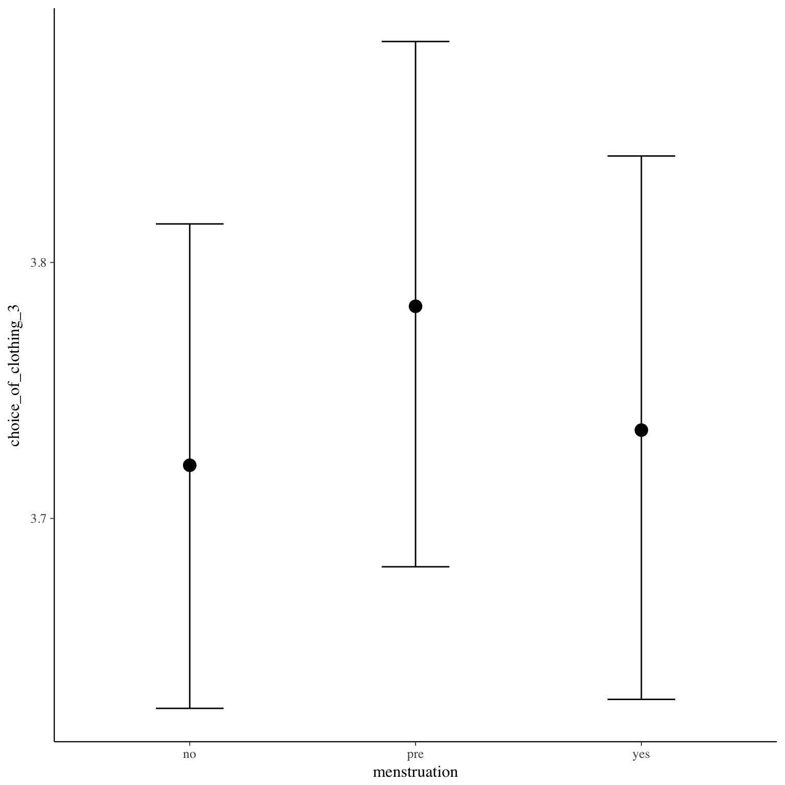
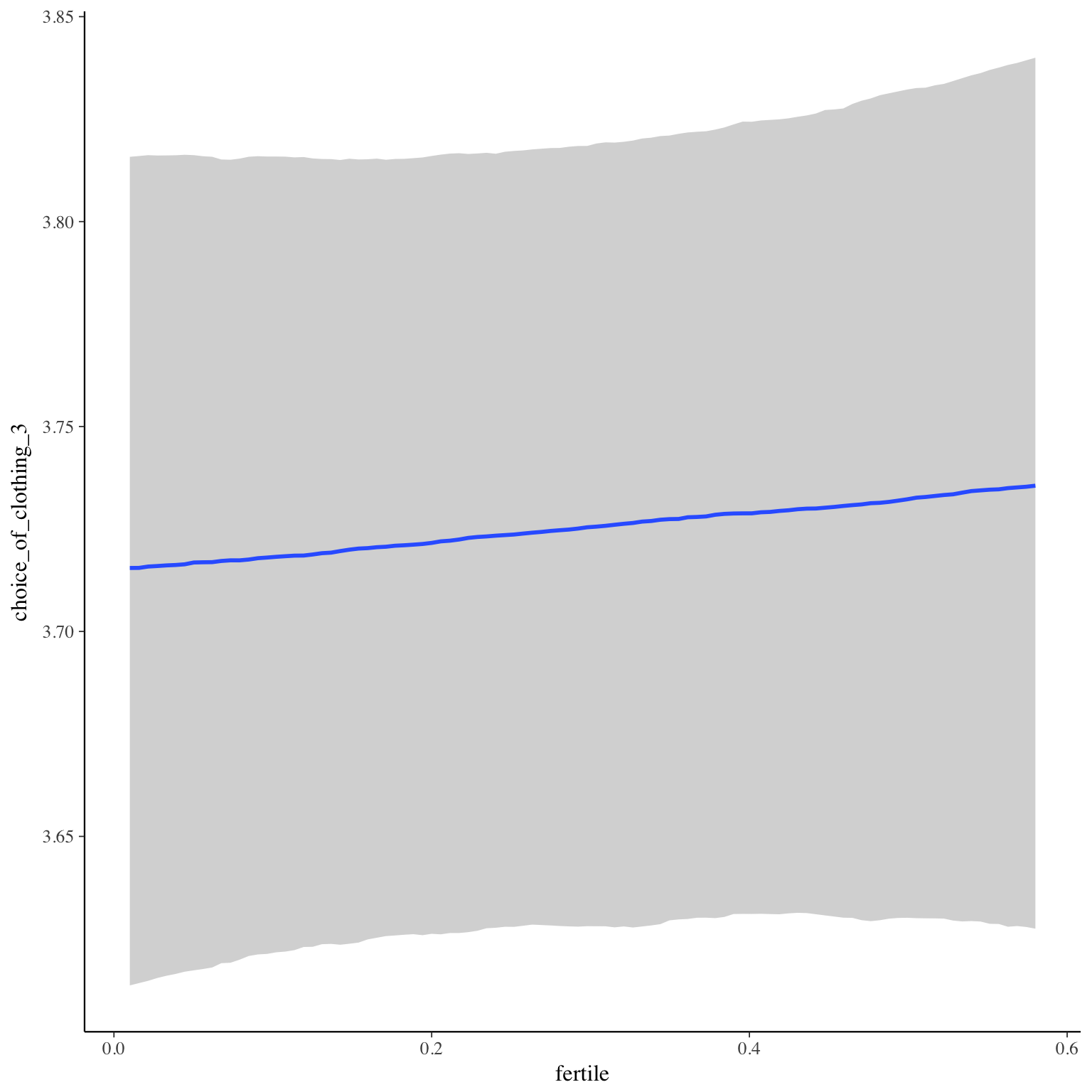
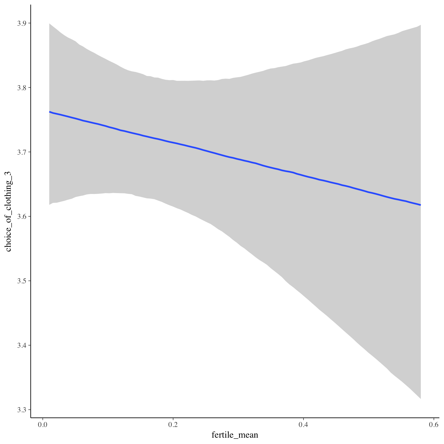
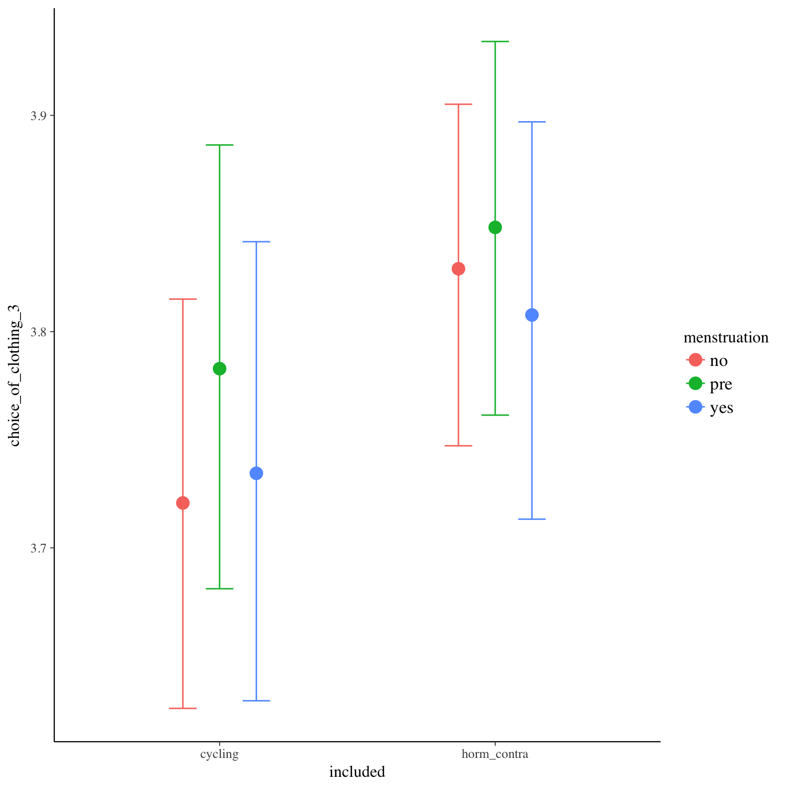
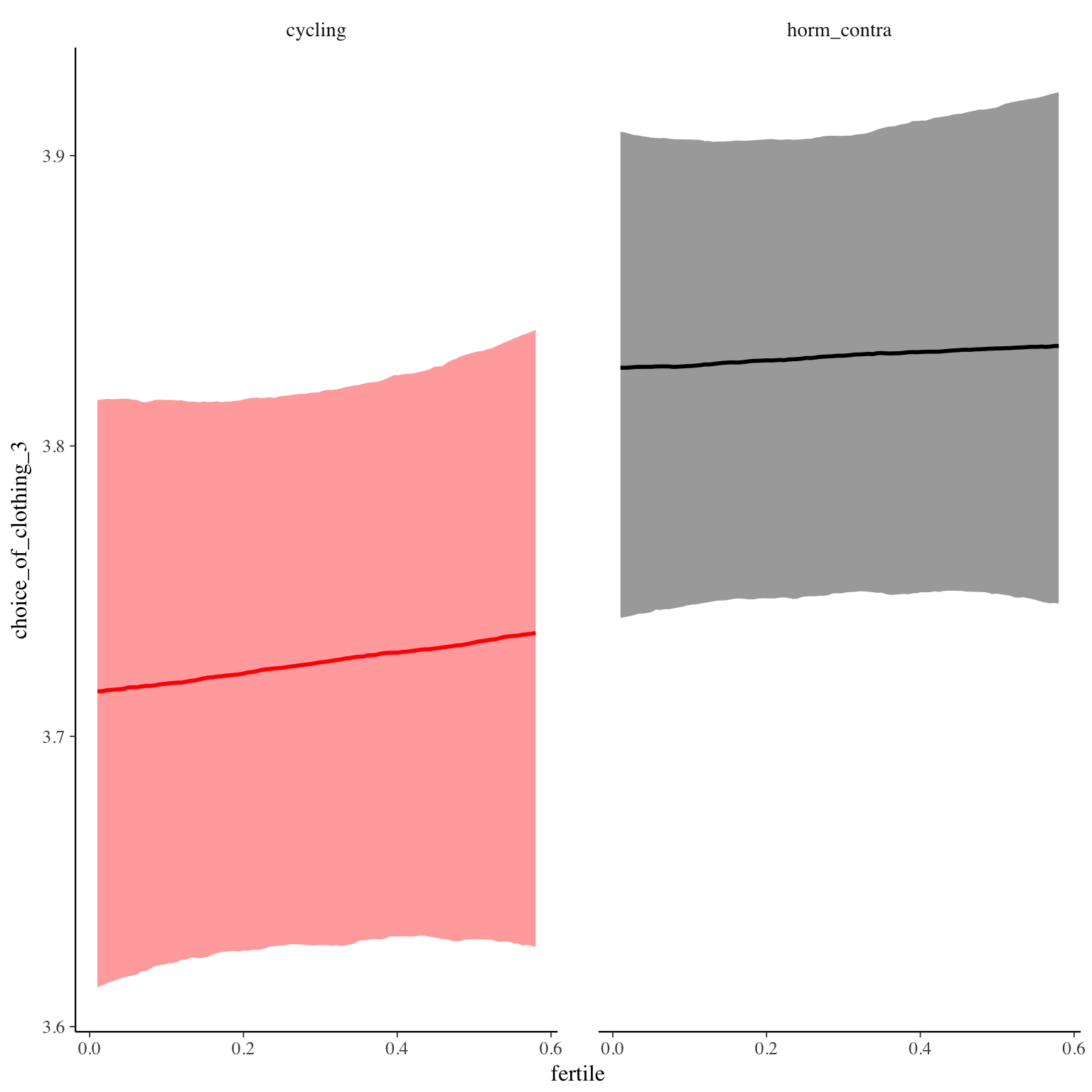
choice_of_clothing_3
Item text:
Sportlich
Item translation:
18. athletic
Choices:
| choice | value | frequency | percent |
|---|---|---|---|
| 1 | Stimme nicht zu | 2782 | 0.09 |
| 2 | Stimme überwiegend nicht zu | 2963 | 0.1 |
| 3 | Stimme eher nicht zu | 5880 | 0.2 |
| 4 | Stimme eher zu | 8896 | 0.3 |
| 5 | Stimme überwiegend zu | 6298 | 0.21 |
| 6 | Stimme voll zu | 3068 | 0.1 |

Model
Model summary
 Family: cumulative(logit)
Formula: choice_of_clothing_3 ~ included * (menstruation + fertile) + fertile_mean + (1 + fertile + menstruation | person)
         disc = 1
   Data: diary (Number of observations: 26554)
Samples: 4 chains, each with iter = 2000; warmup = 1000; thin = 1;
         total post-warmup samples = 4000
    ICs: LOO = 79384.6; WAIC = Not computed

Group-Level Effects:
~person (Number of levels: 1043)
                                     Estimate Est.Error l-95% CI u-95% CI Eff.Sample Rhat
sd(Intercept)                            1.49      0.04     1.41     1.58        885 1.00
sd(fertile)                              0.97      0.15     0.67     1.24        379 1.01
sd(menstruationpre)                      0.46      0.07     0.32     0.58        501 1.00
sd(menstruationyes)                      0.54      0.06     0.40     0.65        433 1.00
cor(Intercept,fertile)                  -0.22      0.09    -0.39    -0.03       4000 1.00
cor(Intercept,menstruationpre)          -0.36      0.09    -0.52    -0.18       4000 1.00
cor(fertile,menstruationpre)             0.24      0.19    -0.16     0.55        326 1.00
cor(Intercept,menstruationyes)          -0.20      0.08    -0.36    -0.04       2353 1.00
cor(fertile,menstruationyes)             0.31      0.16    -0.04     0.59        293 1.00
cor(menstruationpre,menstruationyes)     0.90      0.07     0.73     0.98        504 1.01

Population-Level Effects:
                                    Estimate Est.Error l-95% CI u-95% CI Eff.Sample Rhat
Intercept[1]                           -2.98      0.12    -3.21    -2.74       1008    1
Intercept[2]                           -1.86      0.12    -2.10    -1.63        997    1
Intercept[3]                           -0.55      0.12    -0.78    -0.31        994    1
Intercept[4]                            1.09      0.12     0.86     1.33        993    1
Intercept[5]                            2.83      0.12     2.59     3.07        990    1
includedhorm_contra                     0.18      0.11    -0.03     0.39        548    1
menstruationpre                         0.10      0.06    -0.02     0.22       2095    1
menstruationyes                         0.02      0.06    -0.10     0.14       2580    1
fertile                                 0.06      0.13    -0.19     0.30       2697    1
fertile_mean                           -0.40      0.52    -1.44     0.63        913    1
includedhorm_contra:menstruationpre    -0.07      0.08    -0.22     0.08       2266    1
includedhorm_contra:menstruationyes    -0.06      0.08    -0.22     0.10       2890    1
includedhorm_contra:fertile            -0.04      0.16    -0.34     0.27       2589    1

Samples were drawn using sampling(NUTS). For each parameter, Eff.Sample
is a crude measure of effective sample size, and Rhat is the potential
scale reduction factor on split chains (at convergence, Rhat = 1).
Coefficient plot
Marginal effect plots
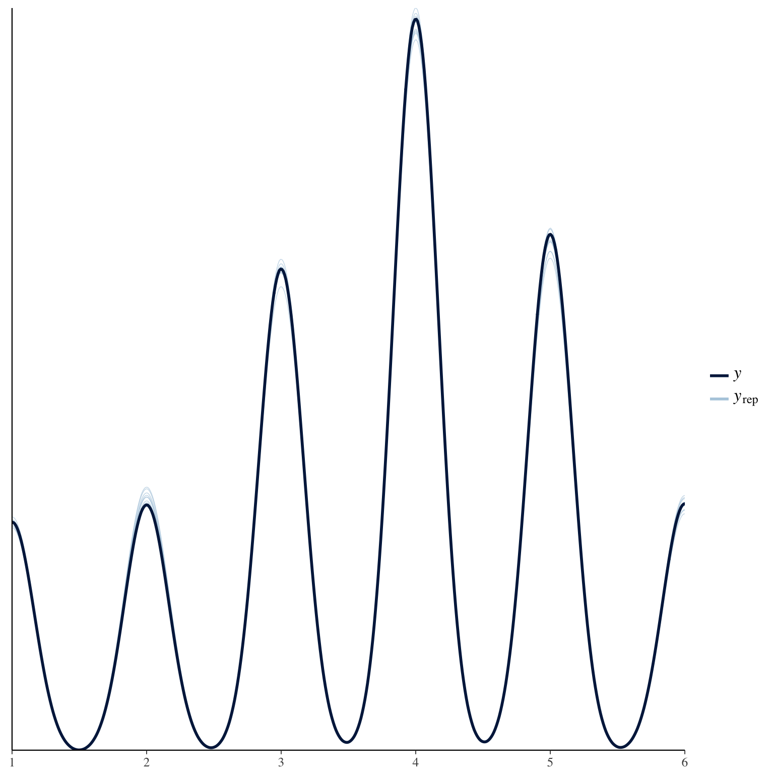
Diagnostics
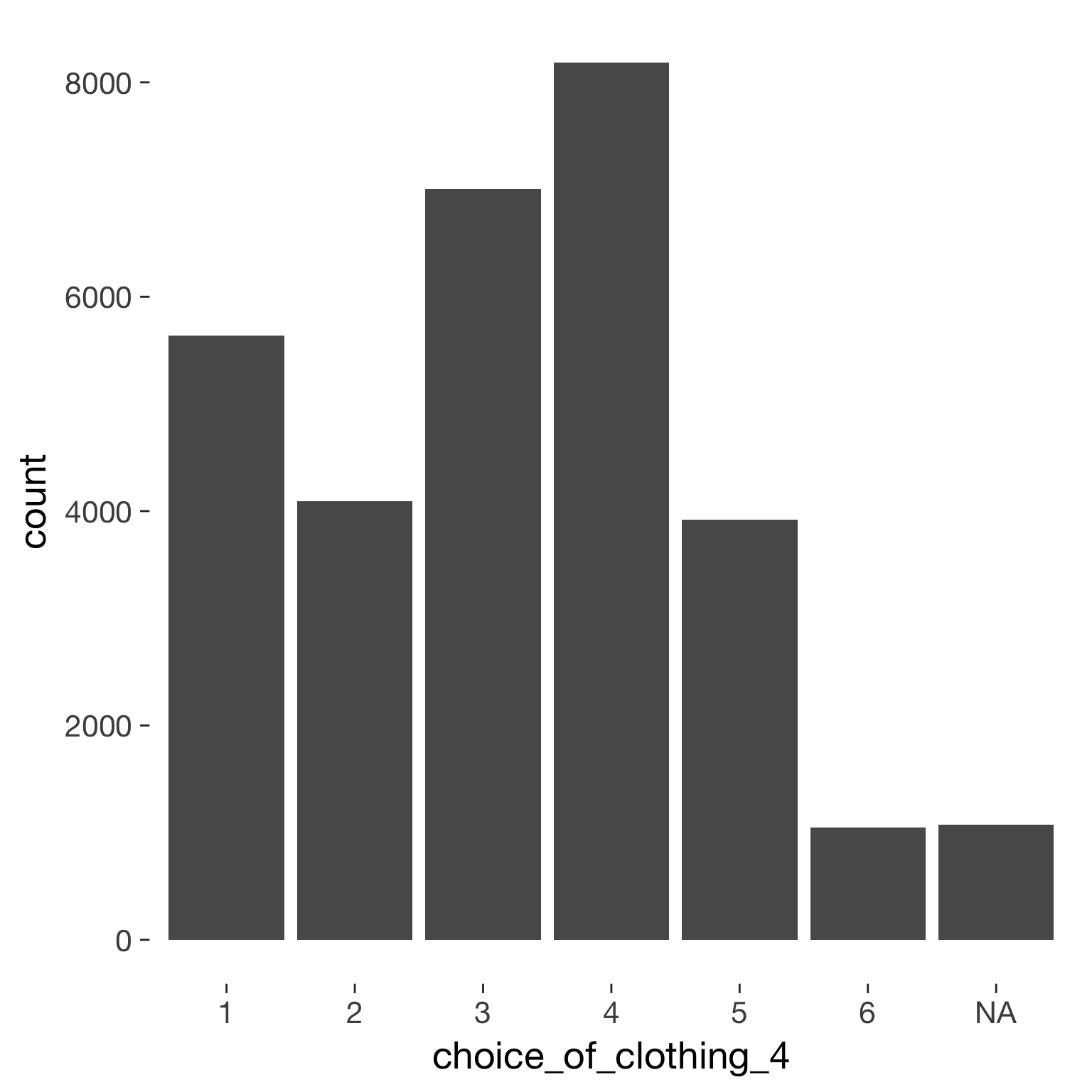
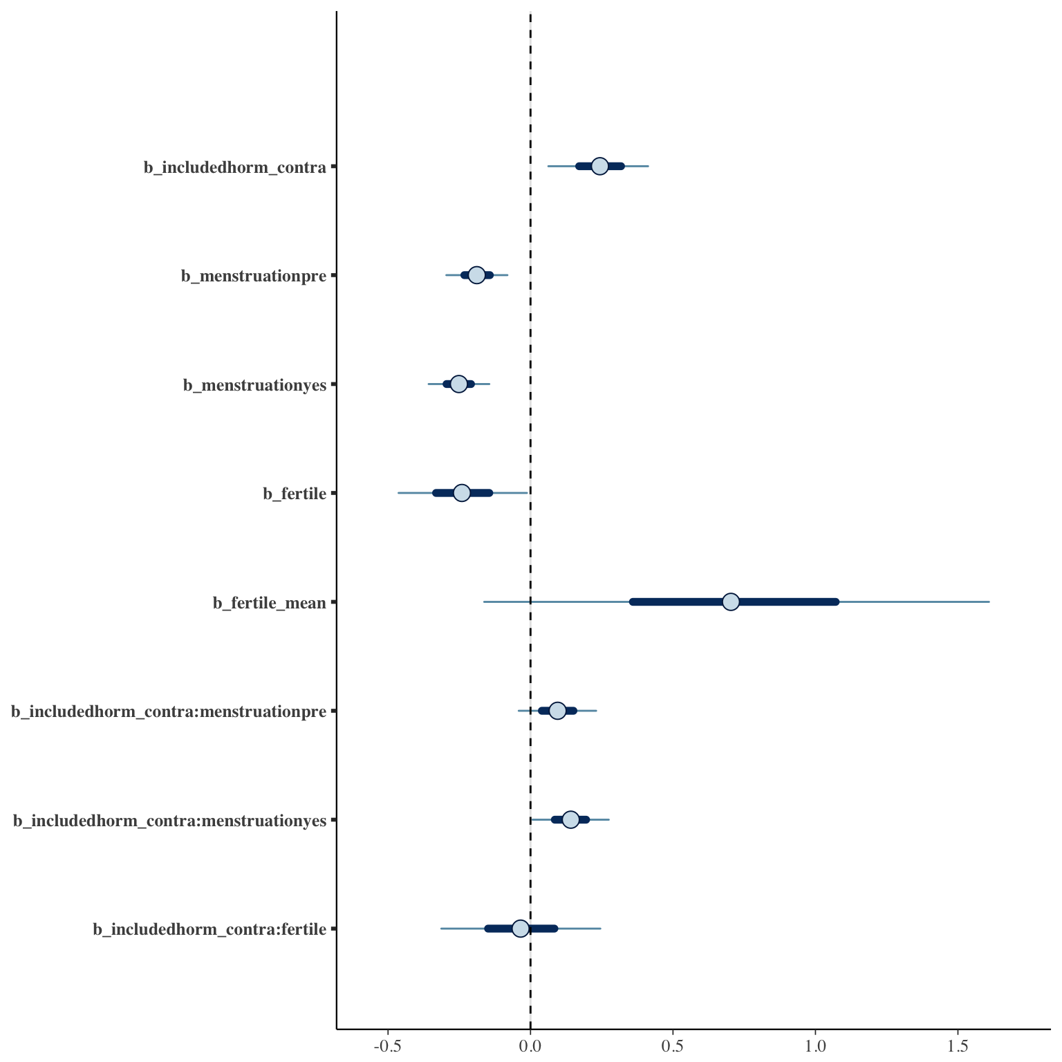
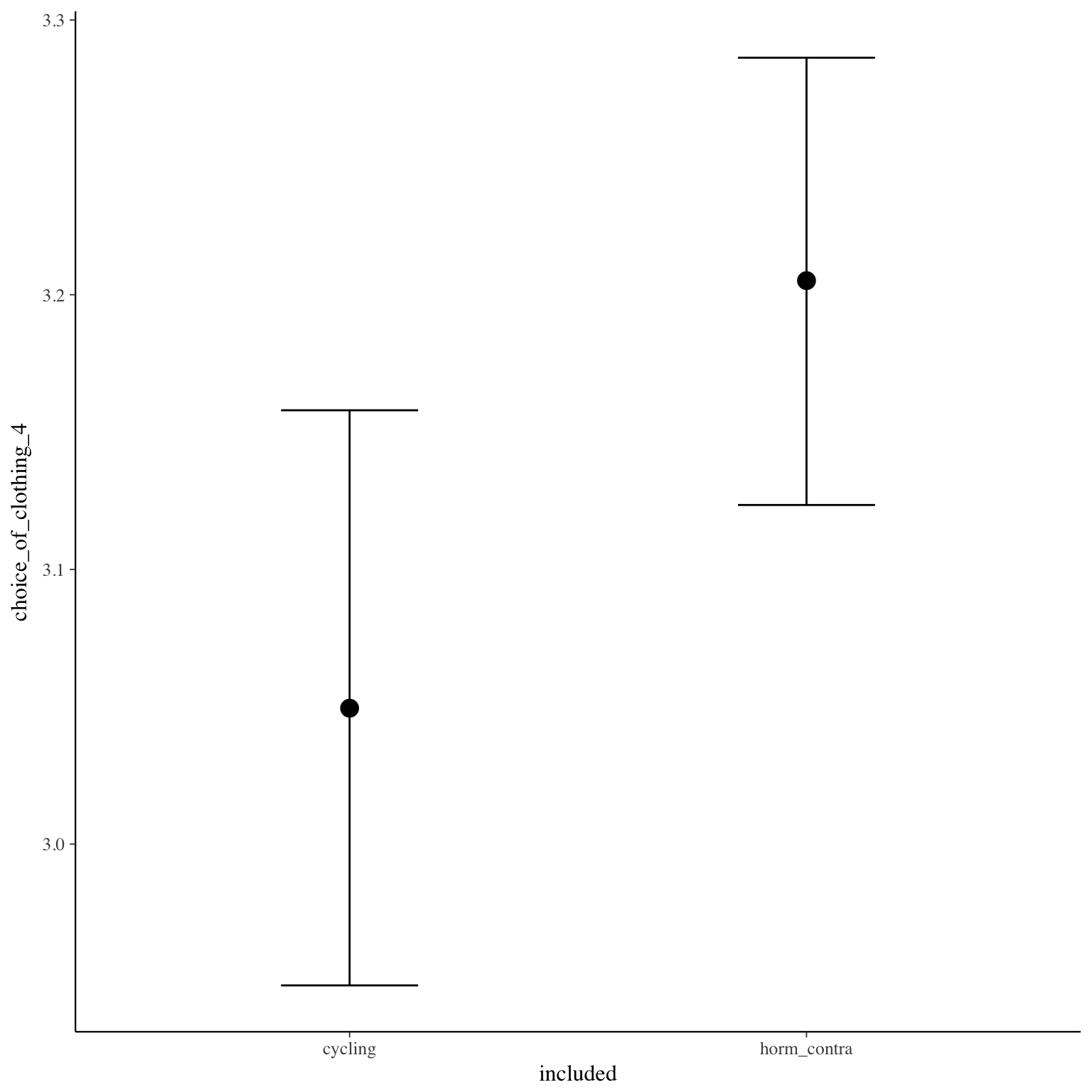
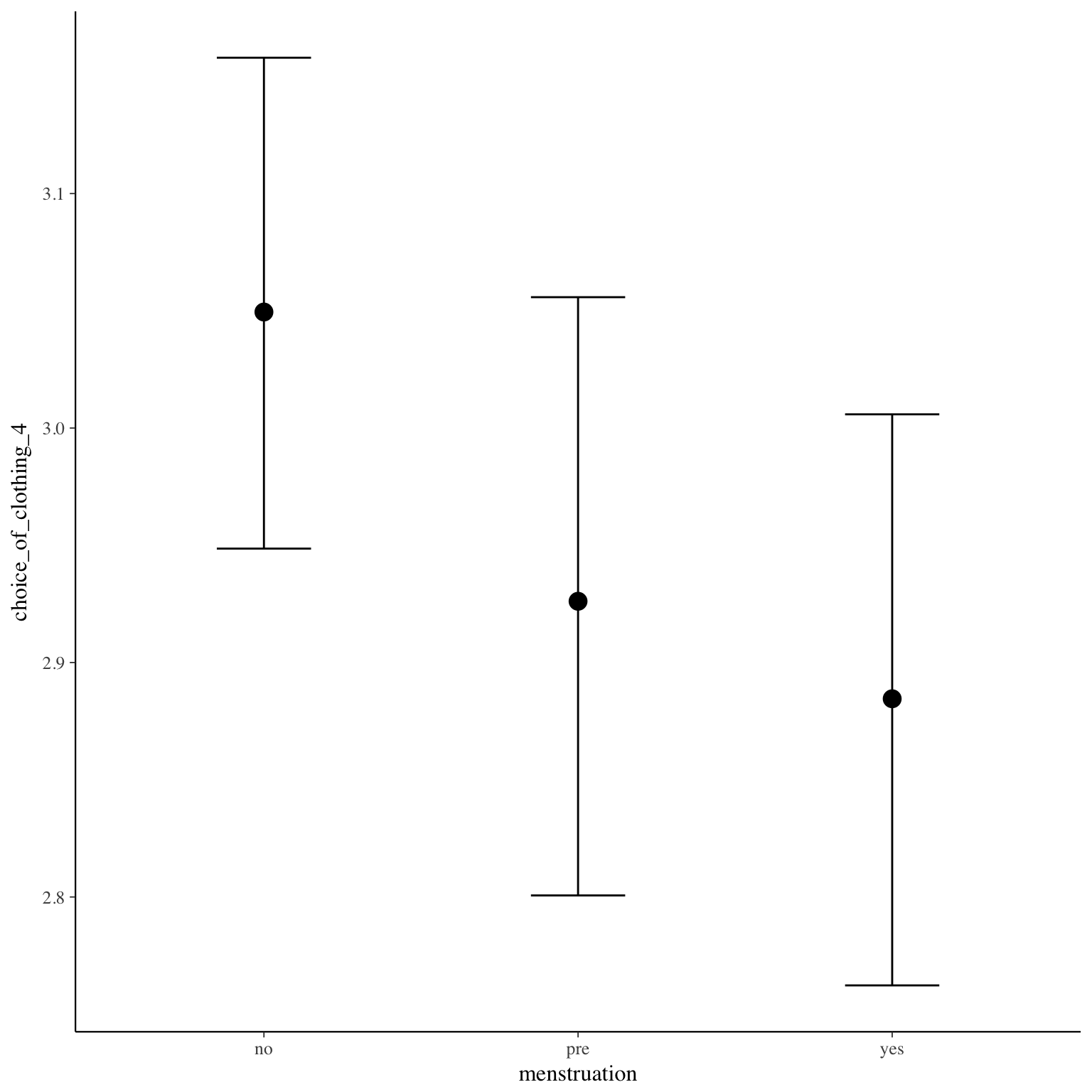
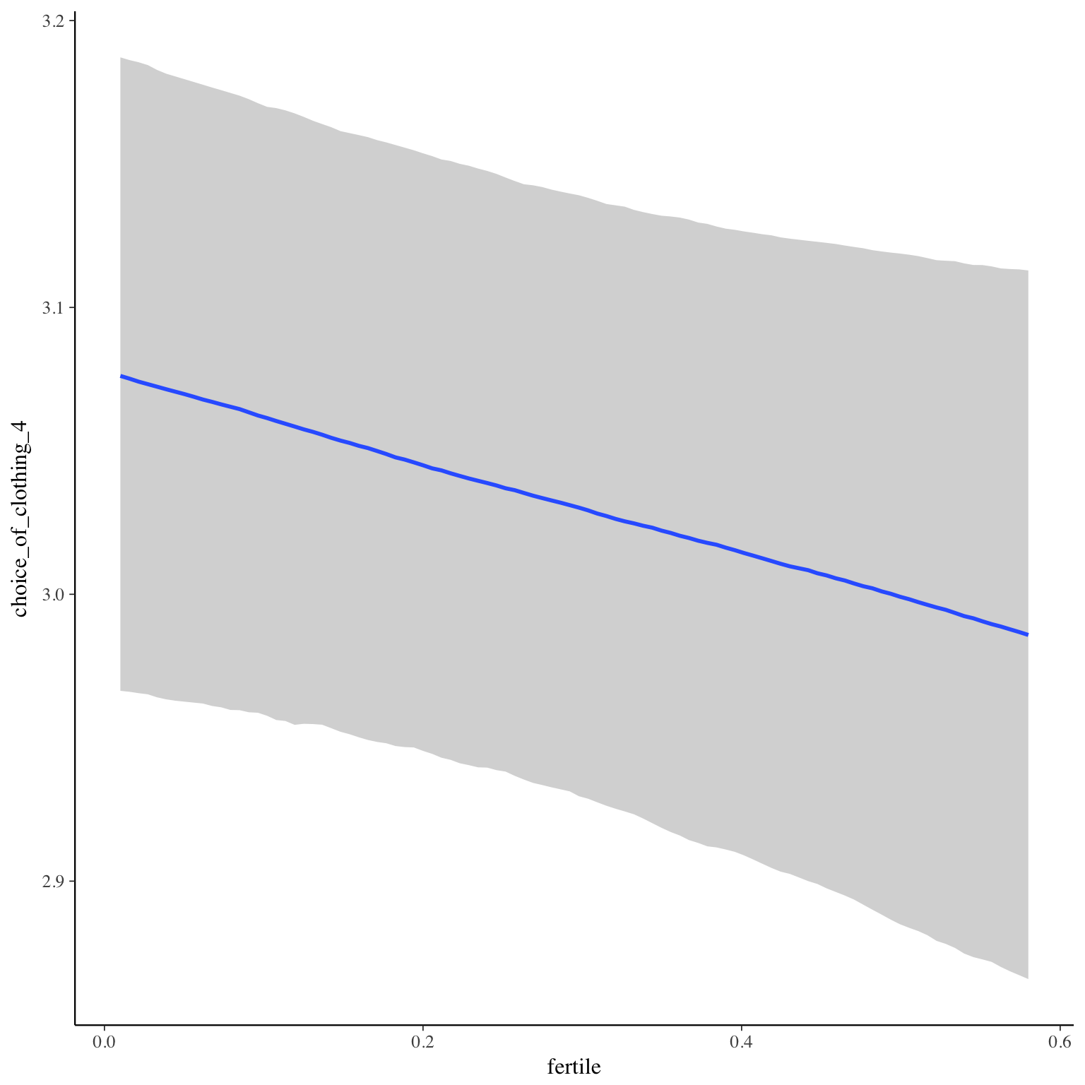
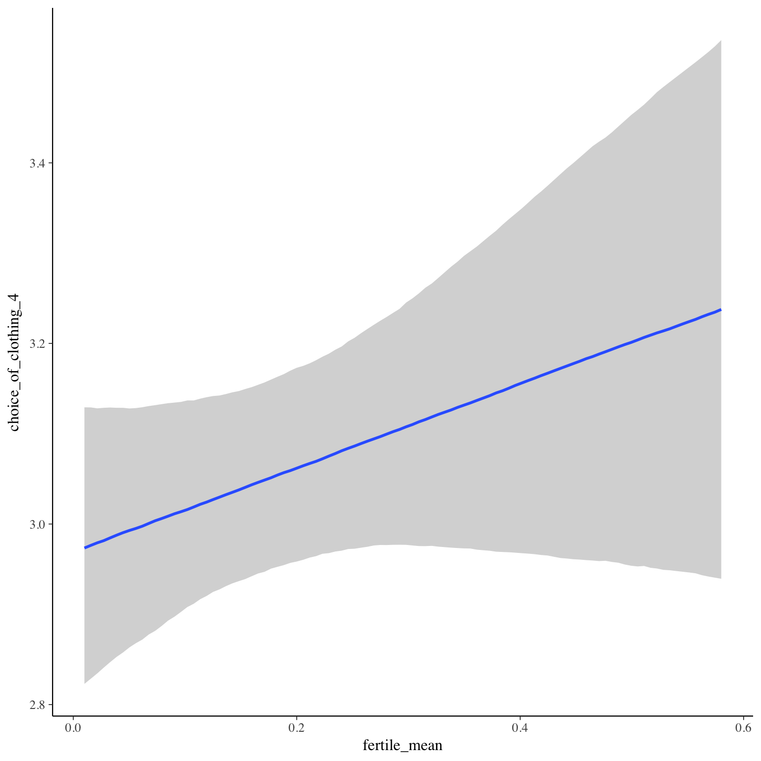
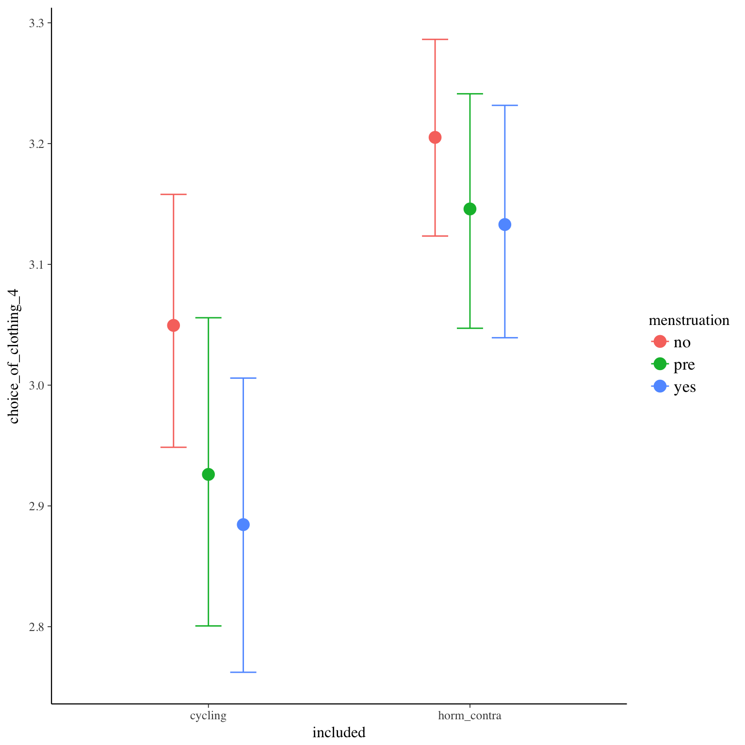
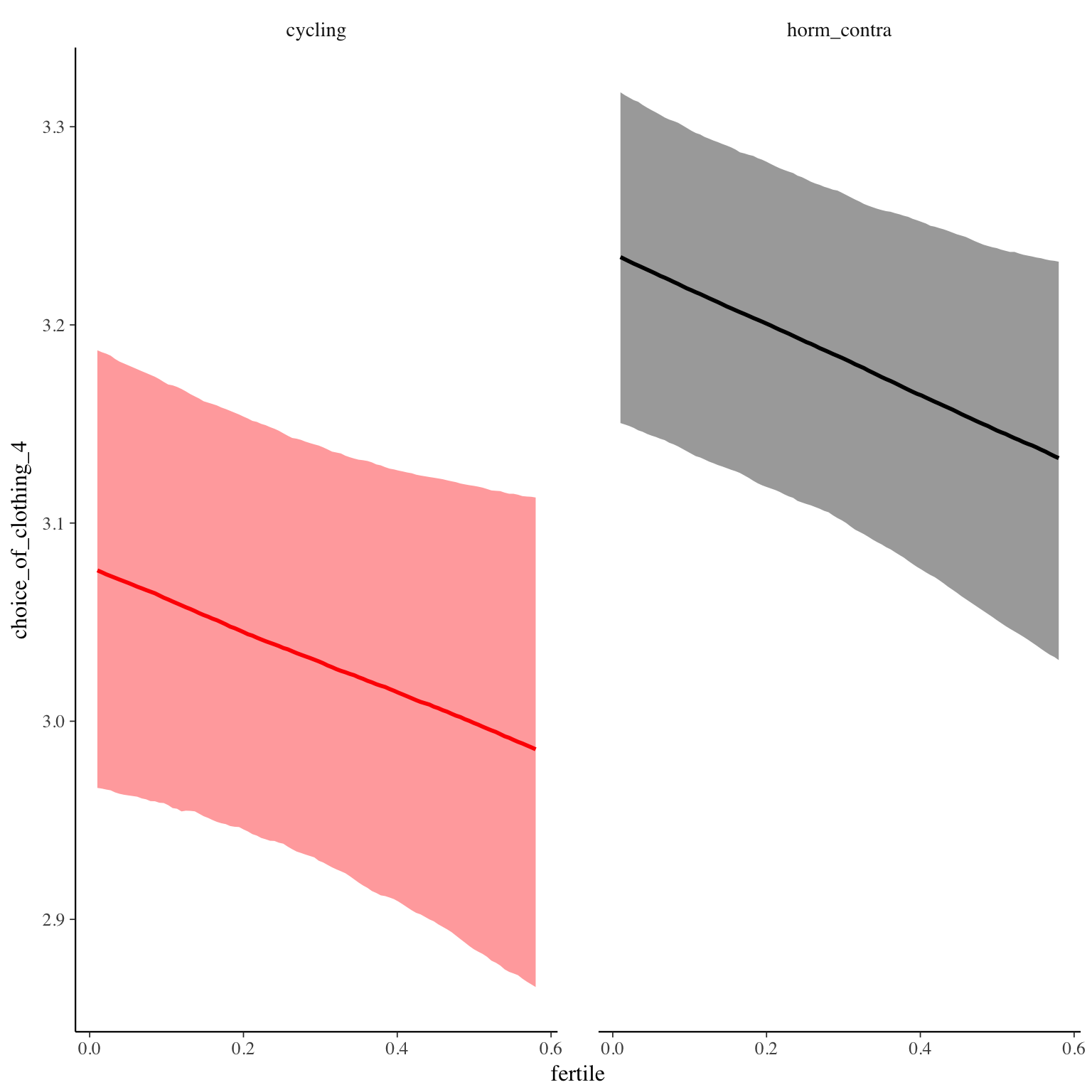
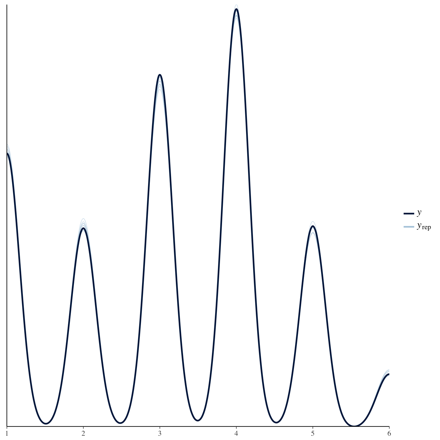
choice_of_clothing_4
Item text:
Sexy
Item translation:
19. sexy
Choices:
| choice | value | frequency | percent |
|---|---|---|---|
| 1 | Stimme nicht zu | 5639 | 0.19 |
| 2 | Stimme überwiegend nicht zu | 4092 | 0.14 |
| 3 | Stimme eher nicht zu | 7002 | 0.23 |
| 4 | Stimme eher zu | 8183 | 0.27 |
| 5 | Stimme überwiegend zu | 3918 | 0.13 |
| 6 | Stimme voll zu | 1050 | 0.04 |
Model
Model summary
 Family: cumulative(logit)
Formula: choice_of_clothing_4 ~ included * (menstruation + fertile) + fertile_mean + (1 + fertile + menstruation | person)
         disc = 1
   Data: diary (Number of observations: 26551)
Samples: 4 chains, each with iter = 2000; warmup = 1000; thin = 1;
         total post-warmup samples = 4000
    ICs: LOO = 77225.54; WAIC = Not computed

Group-Level Effects:
~person (Number of levels: 1043)
                                     Estimate Est.Error l-95% CI u-95% CI Eff.Sample Rhat
sd(Intercept)                            1.48      0.04     1.40     1.57       1019 1.00
sd(fertile)                              1.32      0.13     1.07     1.56        469 1.01
sd(menstruationpre)                      0.52      0.07     0.37     0.65        444 1.00
sd(menstruationyes)                      0.60      0.06     0.47     0.72        755 1.00
cor(Intercept,fertile)                  -0.12      0.08    -0.26     0.04       1413 1.00
cor(Intercept,menstruationpre)          -0.04      0.09    -0.21     0.15       1148 1.00
cor(fertile,menstruationpre)             0.48      0.13     0.19     0.70        490 1.00
cor(Intercept,menstruationyes)          -0.09      0.08    -0.25     0.07       1408 1.00
cor(fertile,menstruationyes)             0.37      0.12     0.10     0.58        457 1.01
cor(menstruationpre,menstruationyes)     0.63      0.12     0.38     0.84        382 1.01

Population-Level Effects:
                                    Estimate Est.Error l-95% CI u-95% CI Eff.Sample Rhat
Intercept[1]                           -1.79      0.12    -2.05    -1.55        675 1.01
Intercept[2]                           -0.77      0.12    -1.02    -0.53        677 1.01
Intercept[3]                            0.58      0.12     0.33     0.82        675 1.01
Intercept[4]                            2.37      0.13     2.11     2.61        683 1.01
Intercept[5]                            4.38      0.13     4.12     4.63        725 1.01
includedhorm_contra                     0.24      0.11     0.02     0.44        551 1.01
menstruationpre                        -0.19      0.07    -0.32    -0.06       2042 1.00
menstruationyes                        -0.25      0.06    -0.38    -0.13       2146 1.00
fertile                                -0.24      0.14    -0.50     0.03       1845 1.00
fertile_mean                            0.71      0.54    -0.33     1.77       1101 1.00
includedhorm_contra:menstruationpre     0.09      0.08    -0.07     0.26       1985 1.00
includedhorm_contra:menstruationyes     0.14      0.08    -0.03     0.30       2149 1.00
includedhorm_contra:fertile            -0.03      0.17    -0.38     0.30       1766 1.00

Samples were drawn using sampling(NUTS). For each parameter, Eff.Sample
is a crude measure of effective sample size, and Rhat is the potential
scale reduction factor on split chains (at convergence, Rhat = 1).
Coefficient plot
Marginal effect plots
Diagnostics
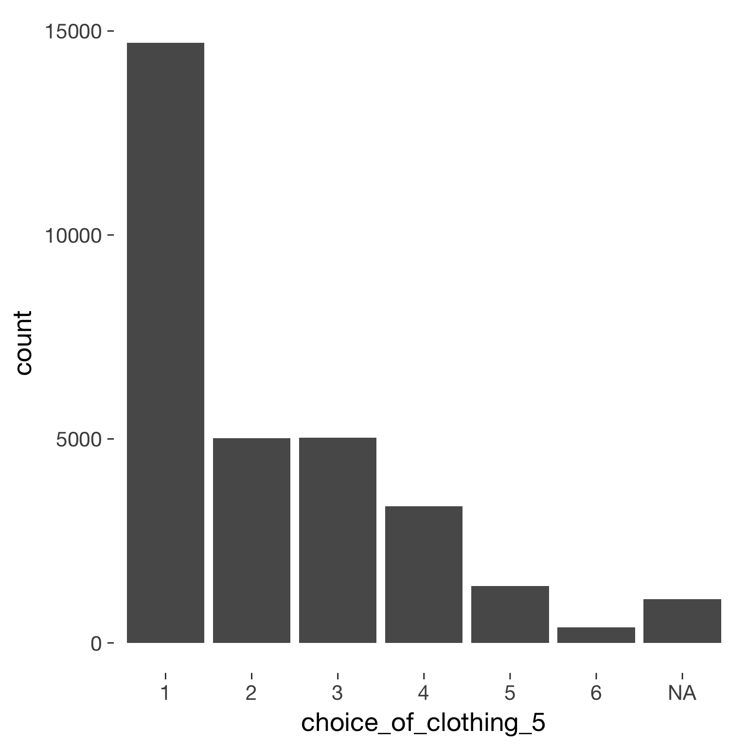
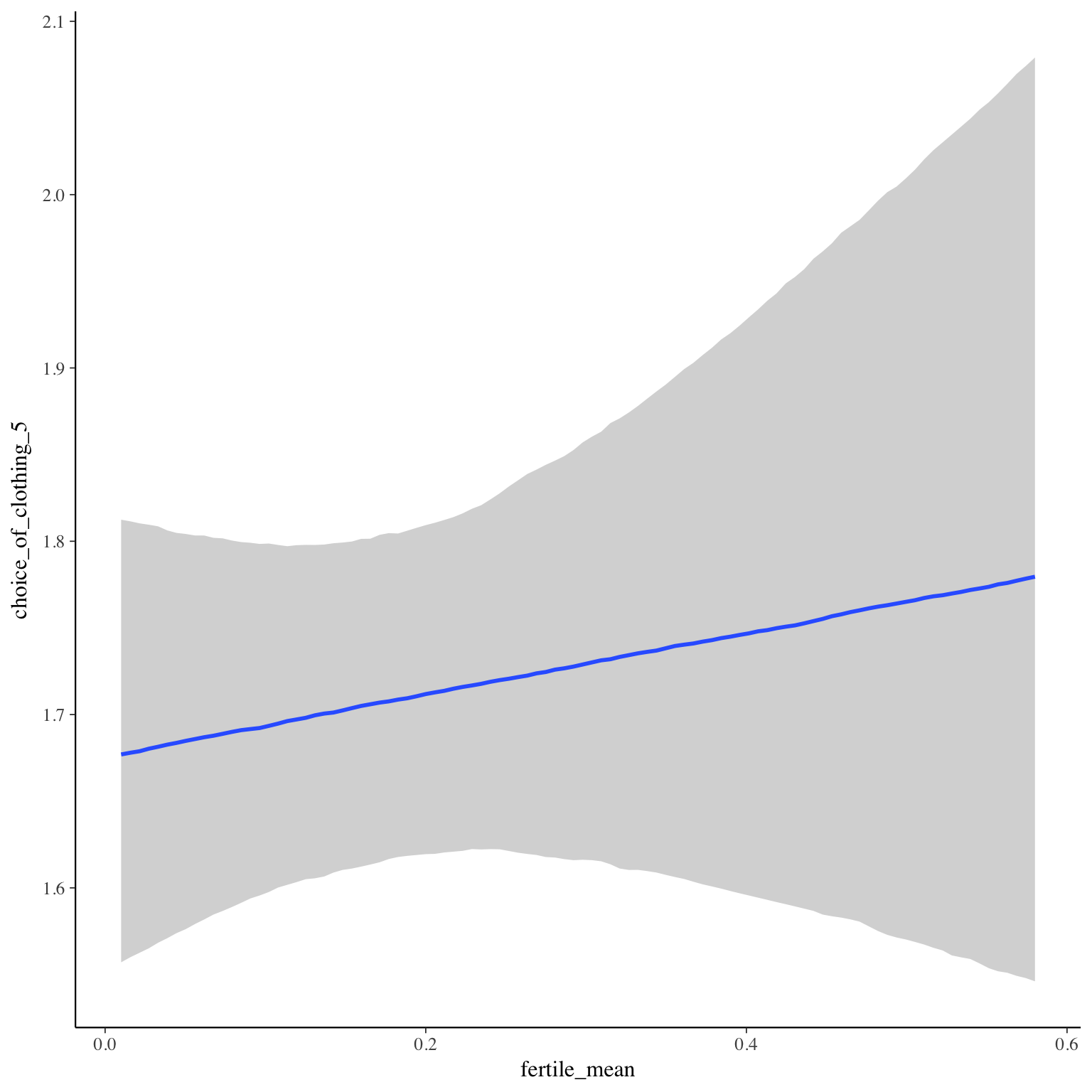
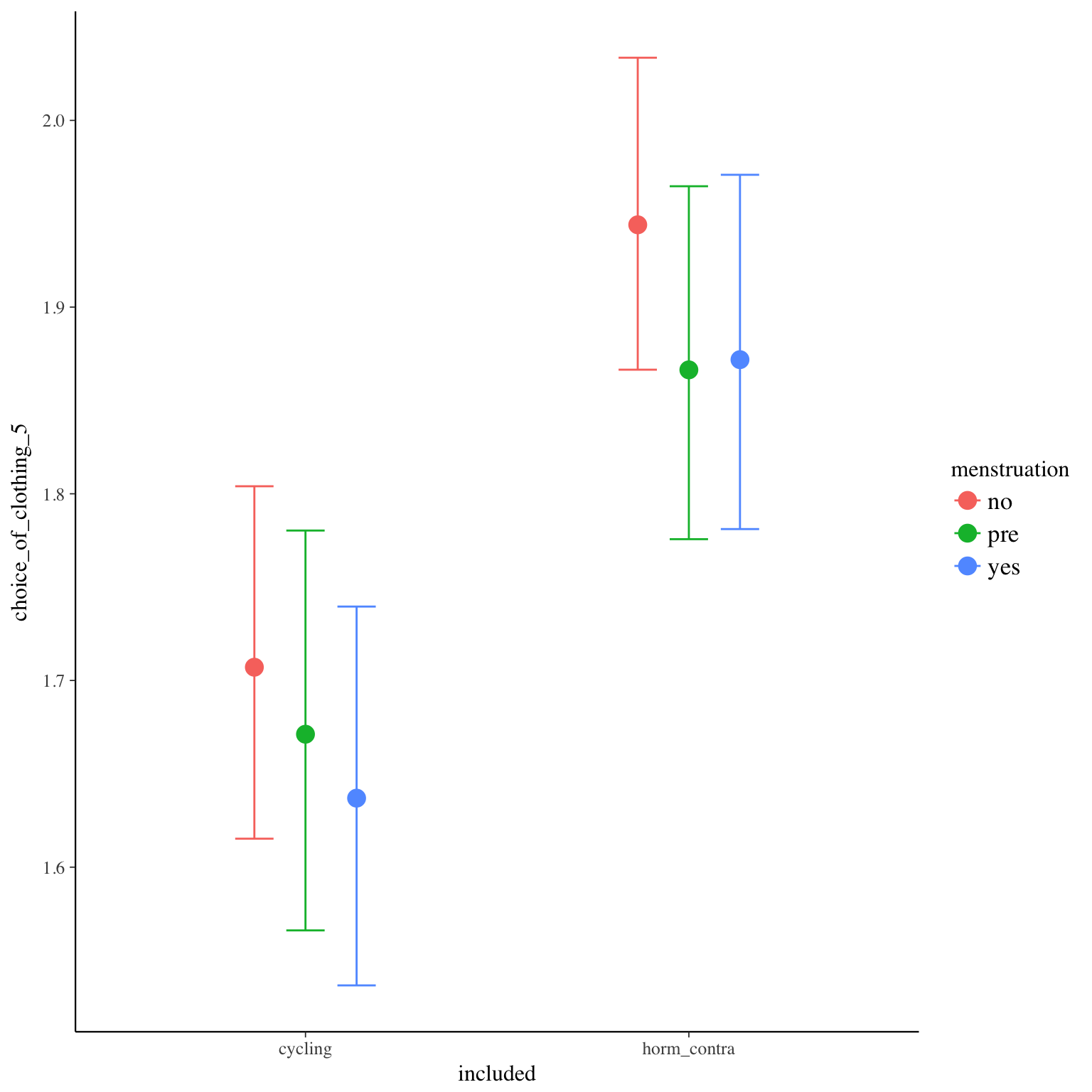
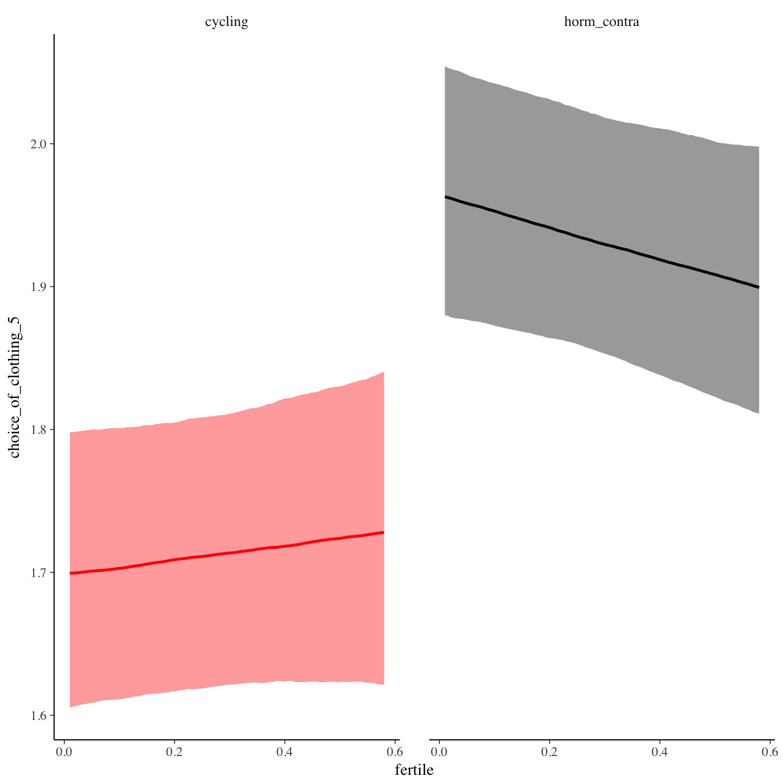
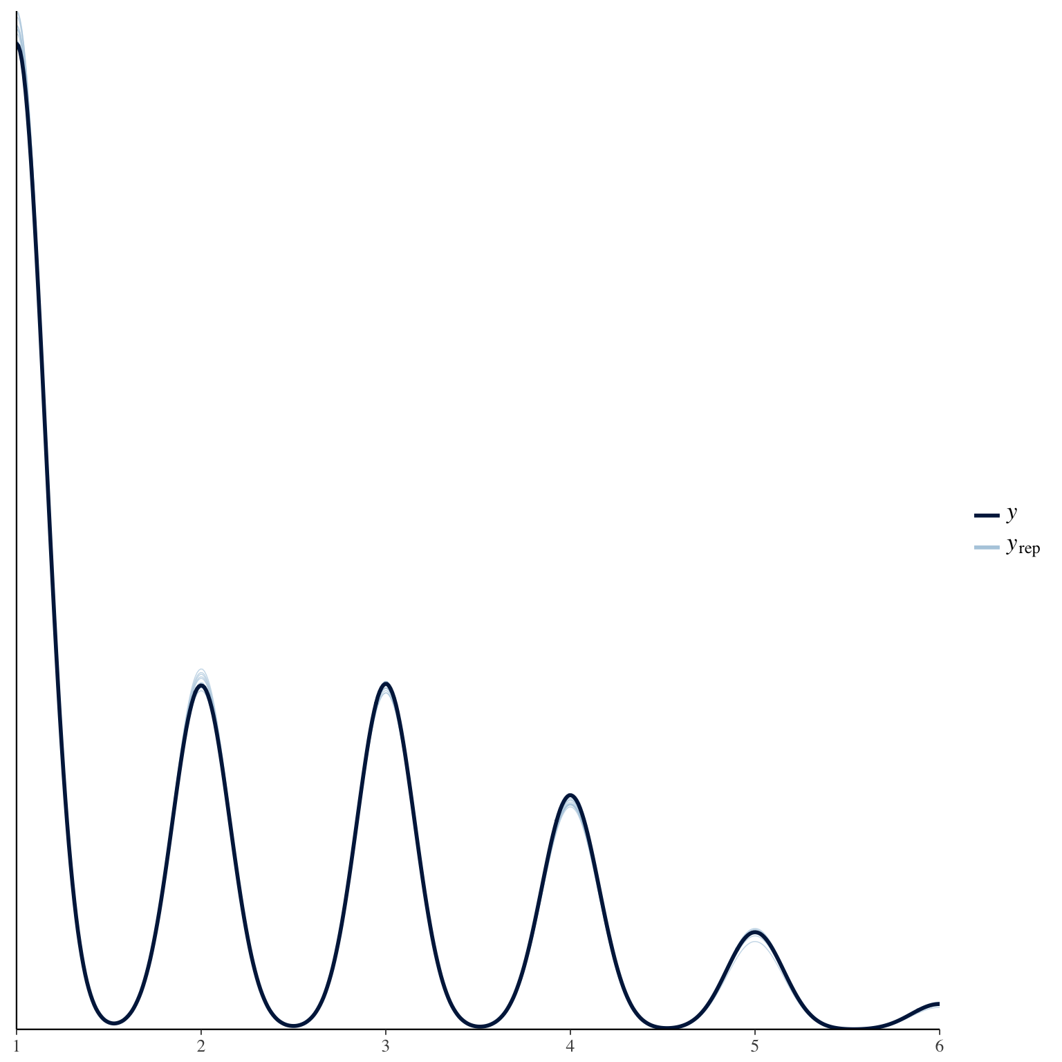
choice_of_clothing_5
Item text:
Glamourös
Item translation:
20. glamorous
Choices:
| choice | value | frequency | percent |
|---|---|---|---|
| 1 | Stimme nicht zu | 14708 | 0.49 |
| 2 | Stimme überwiegend nicht zu | 5023 | 0.17 |
| 3 | Stimme eher nicht zu | 5030 | 0.17 |
| 4 | Stimme eher zu | 3347 | 0.11 |
| 5 | Stimme überwiegend zu | 1400 | 0.05 |
| 6 | Stimme voll zu | 377 | 0.01 |
Model
Model summary
Family: cumulative(logit)
Formula: choice_of_clothing_5 ~ included * (menstruation + fertile) + fertile_mean + (1 + fertile + menstruation | person)
disc = 1
Data: diary (Number of observations: 26552)
Samples: 4 chains, each with iter = 2000; warmup = 1000; thin = 1;
total post-warmup samples = 4000
ICs: LOO = 61988.09; WAIC = Not computed
Group-Level Effects:
~person (Number of levels: 1043)
Estimate Est.Error l-95% CI u-95% CI Eff.Sample Rhat
sd(Intercept) 1.74 0.06 1.64 1.86 511 1.00
sd(fertile) 1.16 0.14 0.87 1.44 354 1.01
sd(menstruationpre) 0.25 0.10 0.04 0.44 215 1.01
sd(menstruationyes) 0.39 0.11 0.11 0.56 183 1.02
cor(Intercept,fertile) -0.02 0.10 -0.22 0.18 1448 1.00
cor(Intercept,menstruationpre) 0.34 0.23 -0.11 0.79 992 1.00
cor(fertile,menstruationpre) -0.08 0.32 -0.73 0.51 360 1.01
cor(Intercept,menstruationyes) 0.12 0.17 -0.18 0.52 469 1.01
cor(fertile,menstruationyes) 0.21 0.22 -0.30 0.59 277 1.01
cor(menstruationpre,menstruationyes) 0.30 0.35 -0.52 0.85 136 1.02
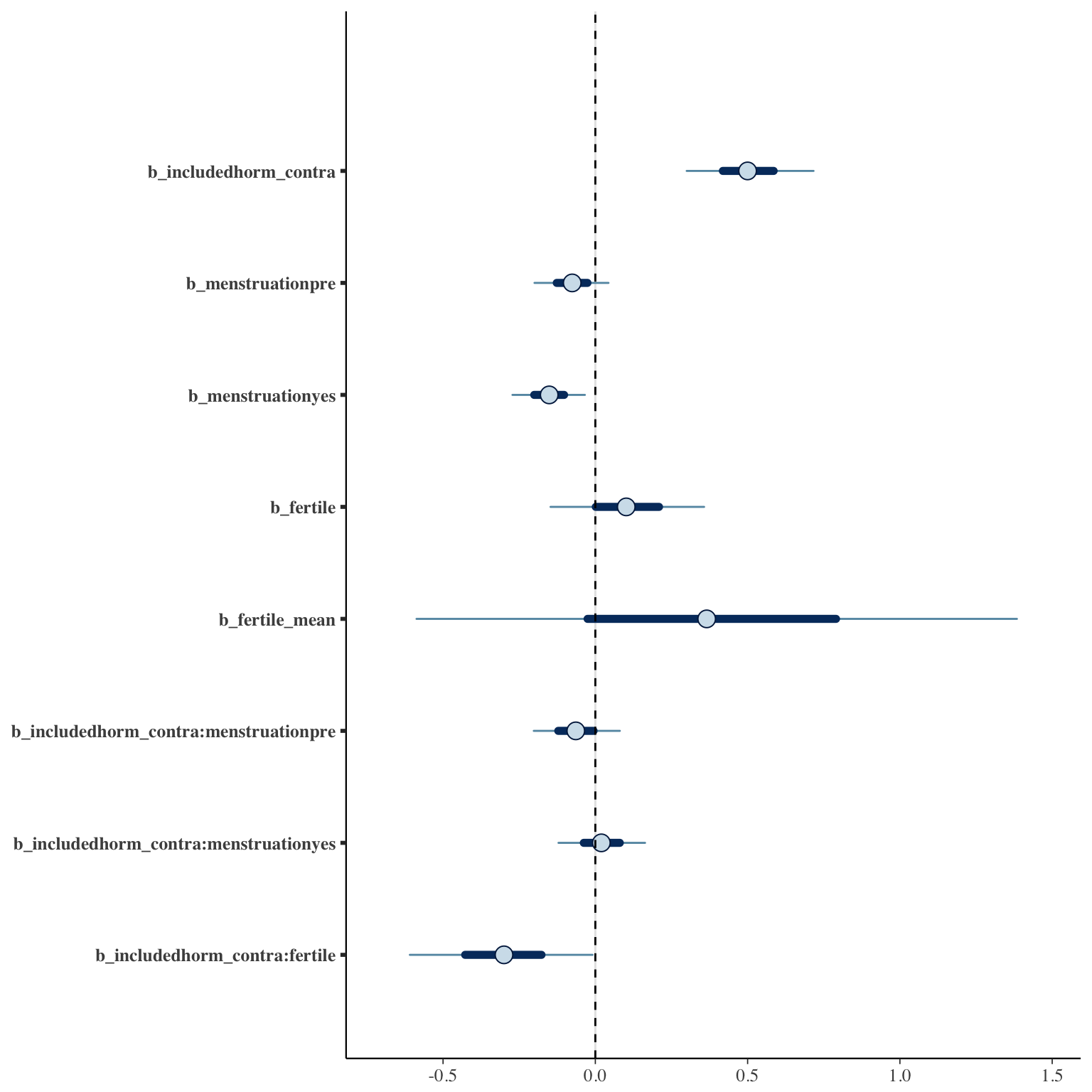
Population-Level Effects:
Estimate Est.Error l-95% CI u-95% CI Eff.Sample Rhat
Intercept[1] 0.40 0.14 0.12 0.68 500 1
Intercept[2] 1.48 0.14 1.19 1.76 504 1
Intercept[3] 2.72 0.14 2.44 3.01 515 1
Intercept[4] 4.18 0.15 3.89 4.47 528 1
Intercept[5] 5.98 0.16 5.67 6.28 681 1
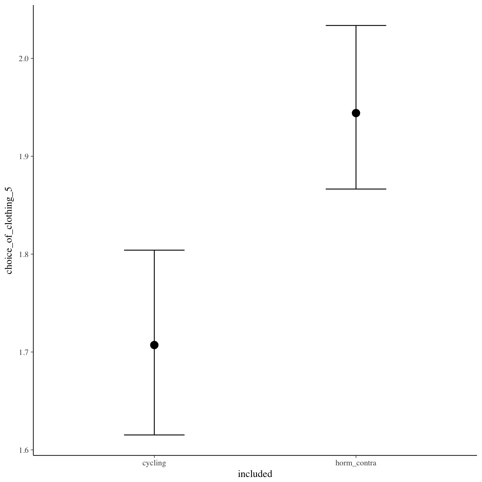
includedhorm_contra 0.50 0.13 0.26 0.76 404 1
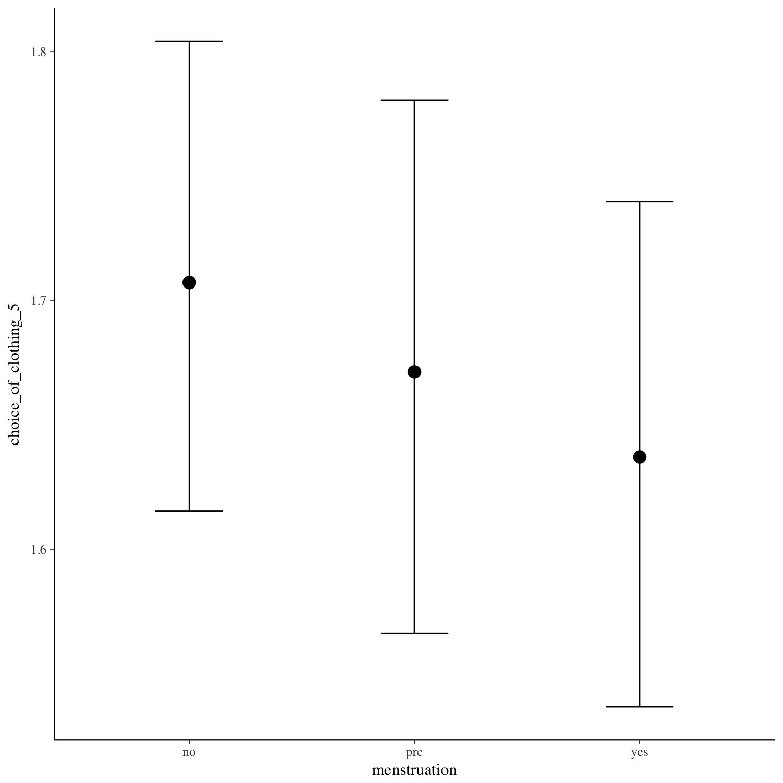
menstruationpre -0.08 0.07 -0.22 0.07 1760 1
menstruationyes -0.15 0.07 -0.29 -0.01 2355 1
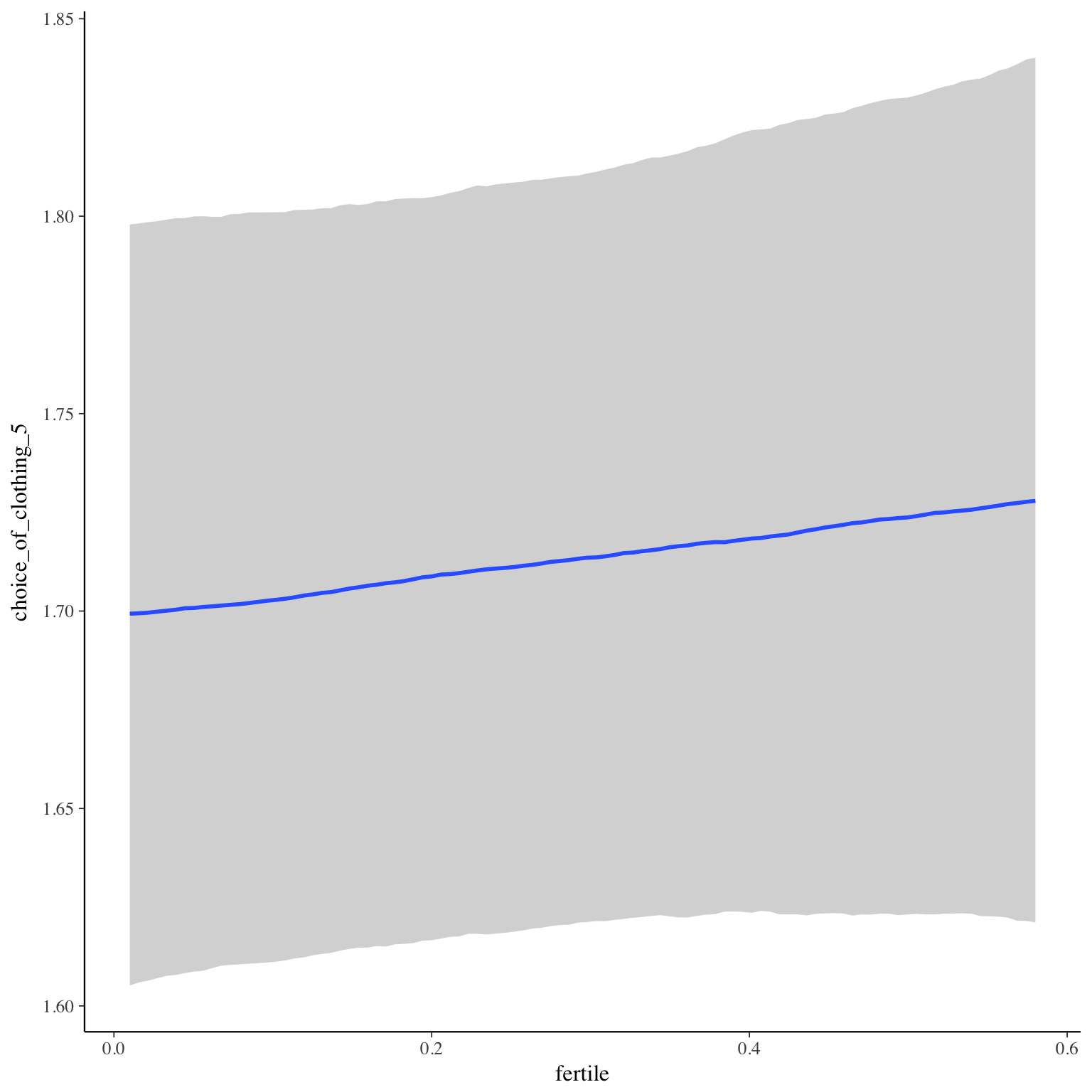
fertile 0.10 0.15 -0.20 0.40 1560 1
fertile_mean 0.38 0.60 -0.75 1.59 1064 1
includedhorm_contra:menstruationpre -0.06 0.09 -0.23 0.11 2070 1
includedhorm_contra:menstruationyes 0.02 0.09 -0.15 0.19 2370 1
includedhorm_contra:fertile -0.30 0.18 -0.66 0.05 1775 1
Samples were drawn using sampling(NUTS). For each parameter, Eff.Sample
is a crude measure of effective sample size, and Rhat is the potential
scale reduction factor on split chains (at convergence, Rhat = 1).
Coefficient plot
Marginal effect plots
Diagnostics
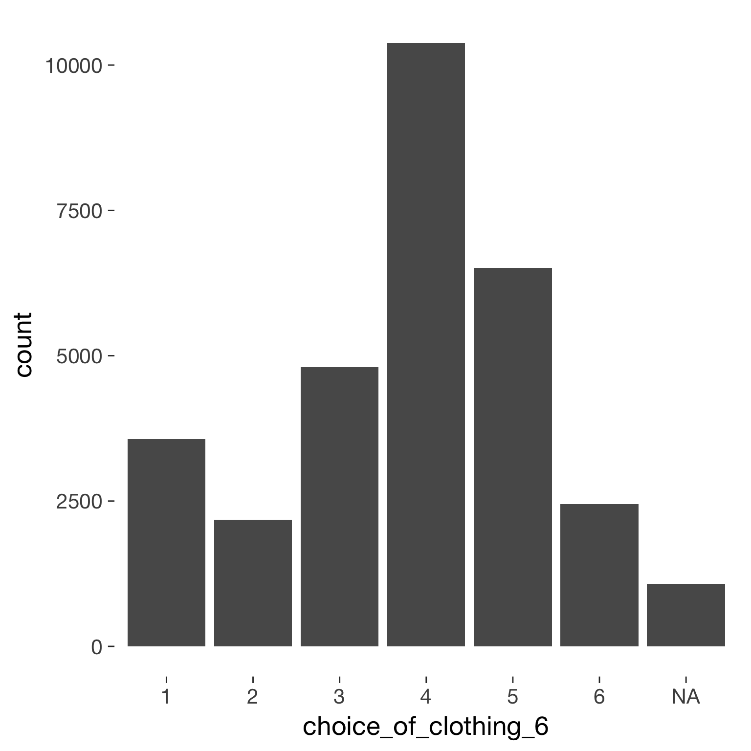
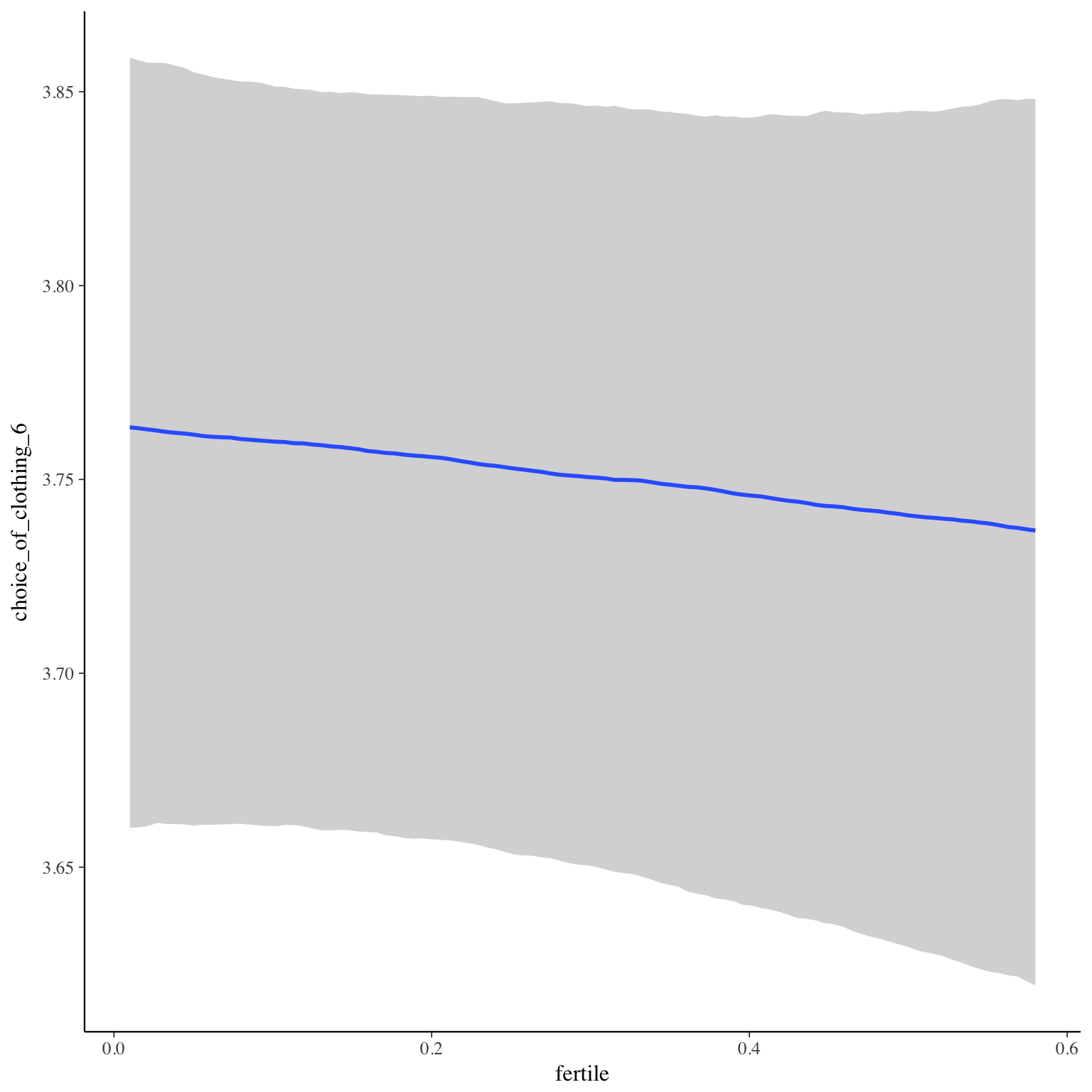
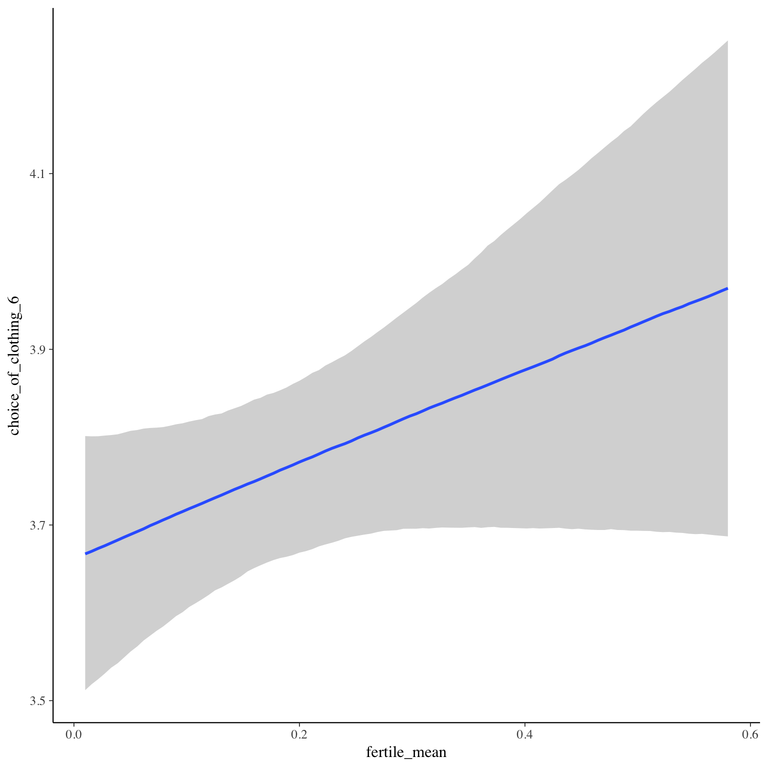
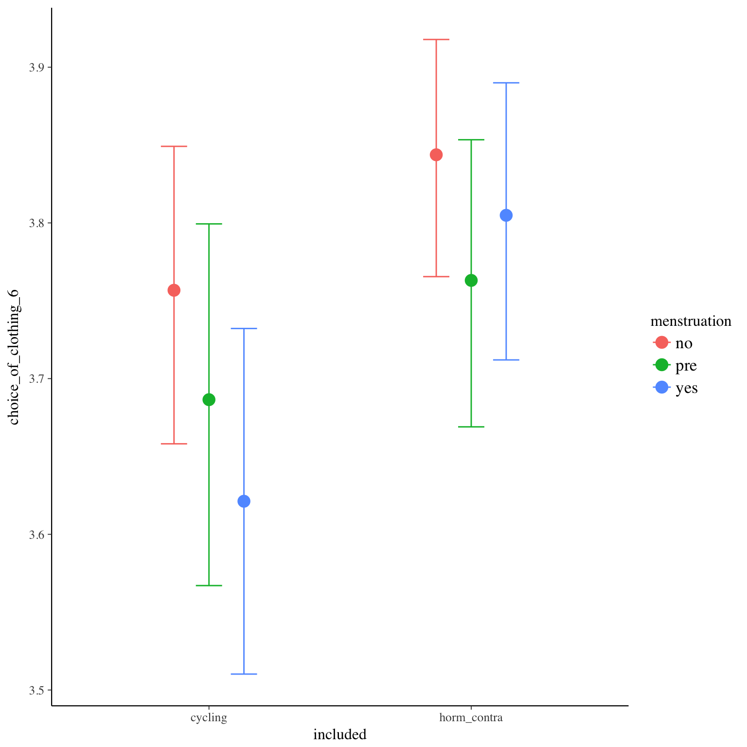
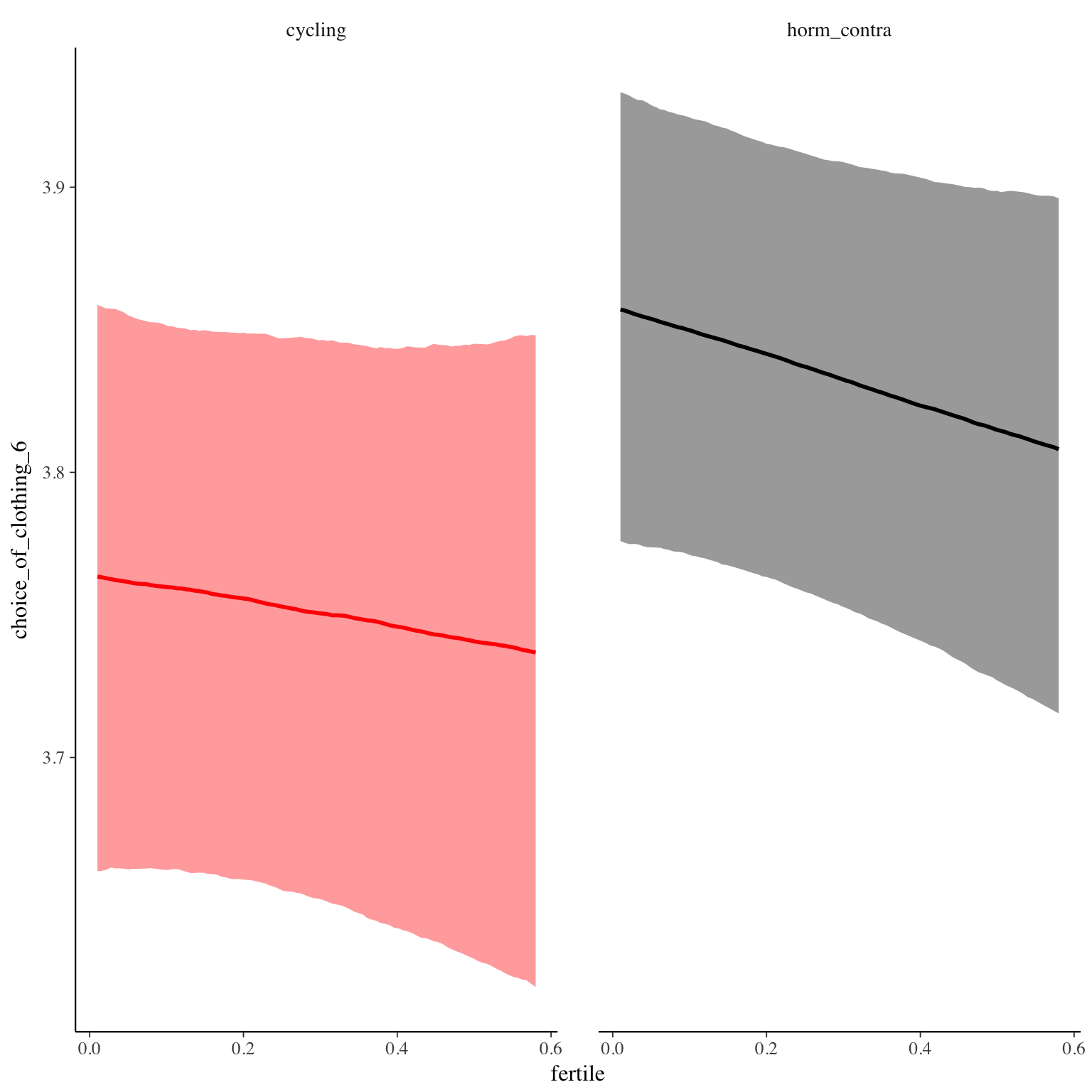
choice_of_clothing_6
Item text:
Figurbetont
Item translation:
21. figure – hugging
Choices:
| choice | value | frequency | percent |
|---|---|---|---|
| 1 | Stimme nicht zu | 3567 | 0.12 |
| 2 | Stimme überwiegend nicht zu | 2175 | 0.07 |
| 3 | Stimme eher nicht zu | 4804 | 0.16 |
| 4 | Stimme eher zu | 10377 | 0.35 |
| 5 | Stimme überwiegend zu | 6510 | 0.22 |
| 6 | Stimme voll zu | 2450 | 0.08 |
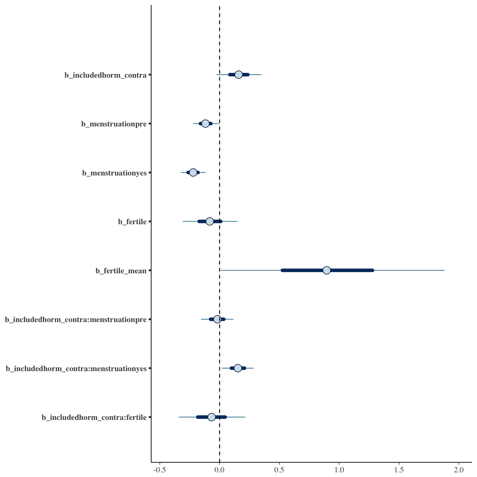
Model
Model summary
 Family: cumulative(logit)
Formula: choice_of_clothing_6 ~ included * (menstruation + fertile) + fertile_mean + (1 + fertile + menstruation | person)
         disc = 1
   Data: diary (Number of observations: 26550)
Samples: 4 chains, each with iter = 2000; warmup = 1000; thin = 1;
         total post-warmup samples = 4000
    ICs: LOO = 75356.62; WAIC = Not computed

Group-Level Effects:
~person (Number of levels: 1043)
                                     Estimate Est.Error l-95% CI u-95% CI Eff.Sample Rhat
sd(Intercept)                            1.56      0.05     1.47     1.67        840 1.00
sd(fertile)                              1.22      0.12     0.97     1.46        479 1.01
sd(menstruationpre)                      0.50      0.07     0.35     0.63        456 1.01
sd(menstruationyes)                      0.50      0.07     0.37     0.63        615 1.00
cor(Intercept,fertile)                  -0.08      0.08    -0.24     0.09       1502 1.00
cor(Intercept,menstruationpre)          -0.14      0.09    -0.31     0.06       1903 1.00
cor(fertile,menstruationpre)             0.43      0.14     0.13     0.66        474 1.00
cor(Intercept,menstruationyes)          -0.23      0.09    -0.39    -0.06       2583 1.00
cor(fertile,menstruationyes)             0.27      0.15    -0.05     0.53        316 1.01
cor(menstruationpre,menstruationyes)     0.71      0.13     0.43     0.95        269 1.01

Population-Level Effects:
                                    Estimate Est.Error l-95% CI u-95% CI Eff.Sample Rhat
Intercept[1]                           -2.54      0.13    -2.78    -2.28        536 1.02
Intercept[2]                           -1.78      0.13    -2.03    -1.52        633 1.02
Intercept[3]                           -0.63      0.13    -0.87    -0.37        630 1.02
Intercept[4]                            1.38      0.13     1.13     1.64        628 1.02
Intercept[5]                            3.43      0.13     3.19     3.70        643 1.01
includedhorm_contra                     0.16      0.11    -0.06     0.38        469 1.01
menstruationpre                        -0.12      0.06    -0.24     0.01       1972 1.00
menstruationyes                        -0.22      0.06    -0.34    -0.10       2008 1.00
fertile                                -0.08      0.14    -0.35     0.20       2118 1.00
fertile_mean                            0.91      0.57    -0.17     2.09        946 1.00
includedhorm_contra:menstruationpre    -0.02      0.08    -0.18     0.14       1840 1.00
includedhorm_contra:menstruationyes     0.15      0.08     0.00     0.31       1724 1.00
includedhorm_contra:fertile            -0.07      0.17    -0.39     0.27       1874 1.00

Samples were drawn using sampling(NUTS). For each parameter, Eff.Sample
is a crude measure of effective sample size, and Rhat is the potential
scale reduction factor on split chains (at convergence, Rhat = 1).
Coefficient plot
Marginal effect plots
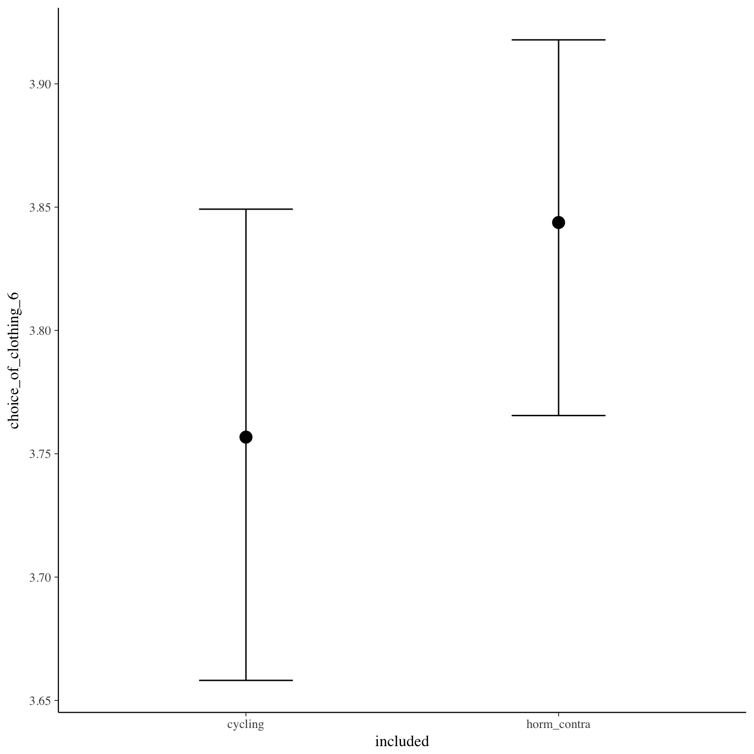
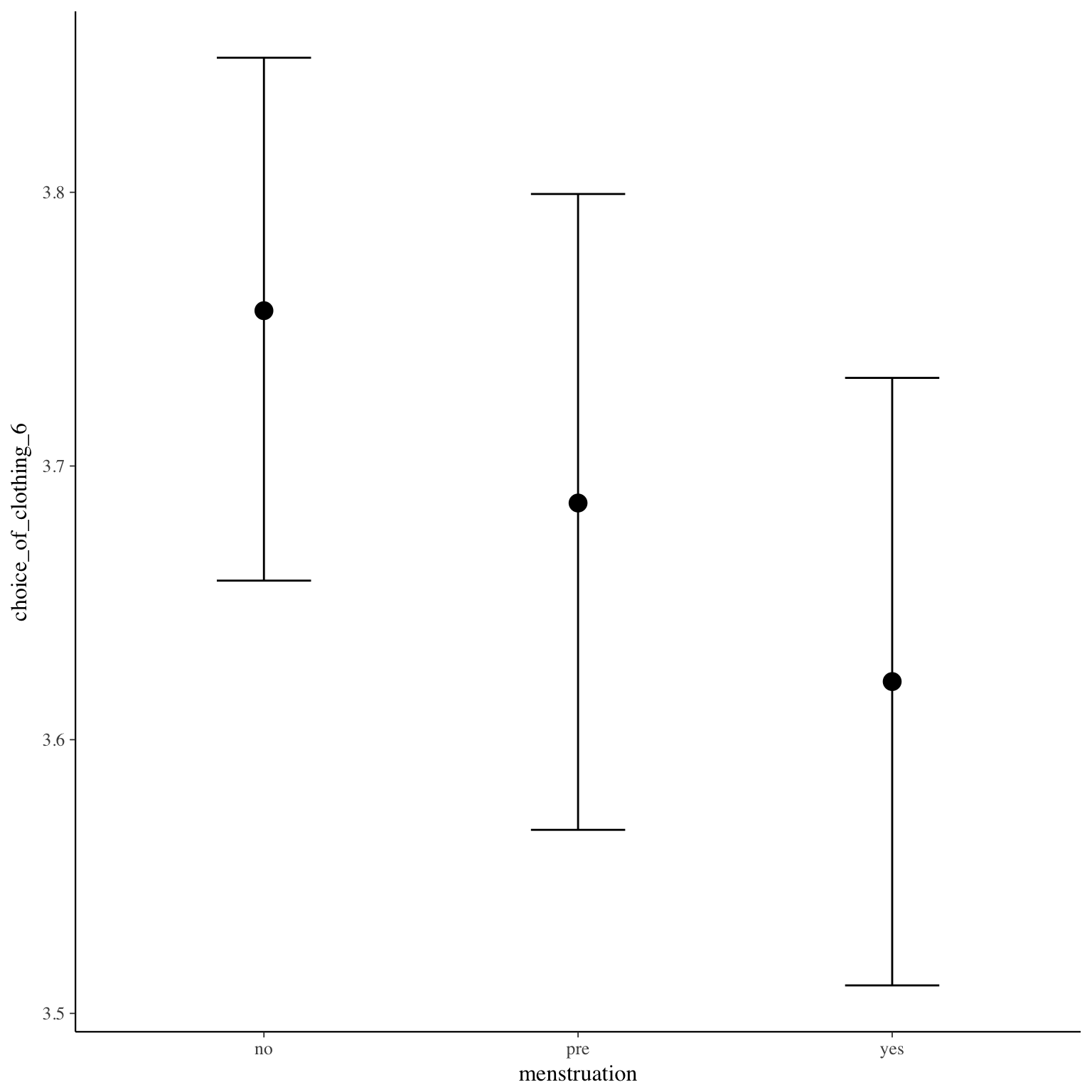
Diagnostics
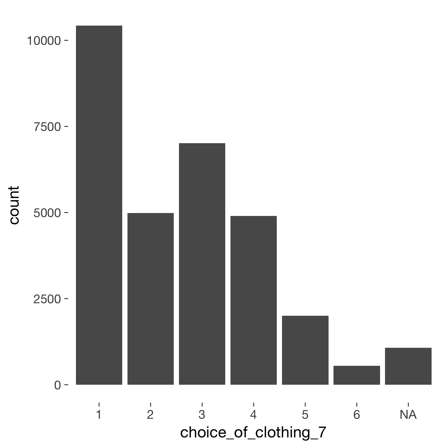
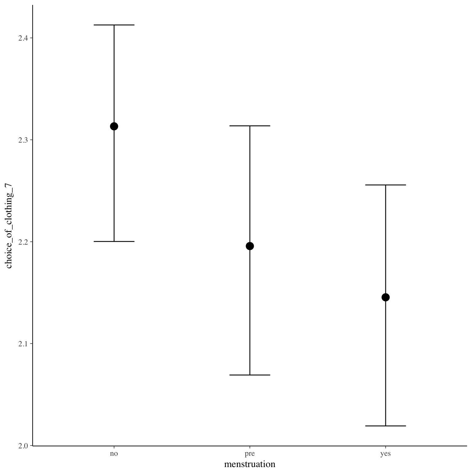
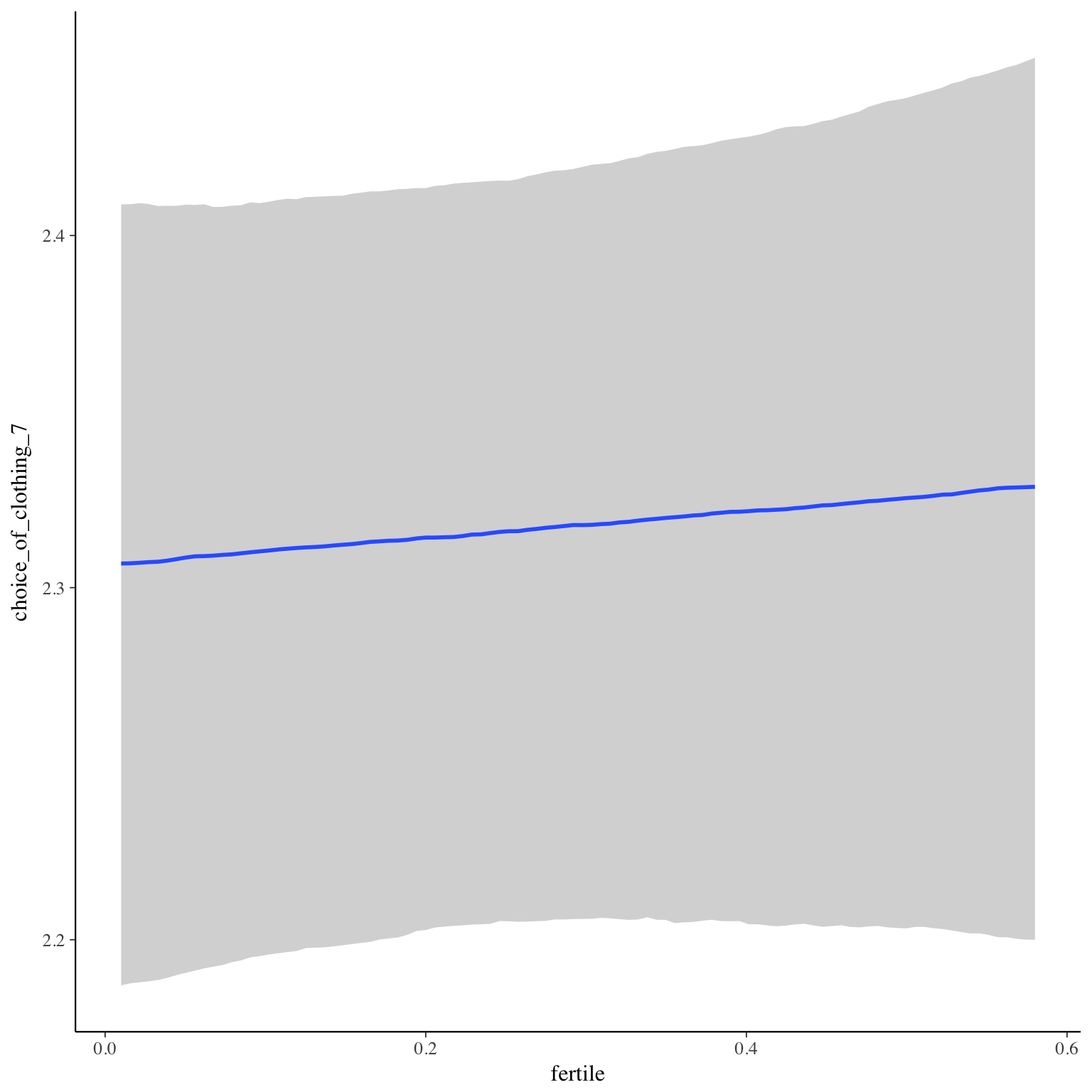
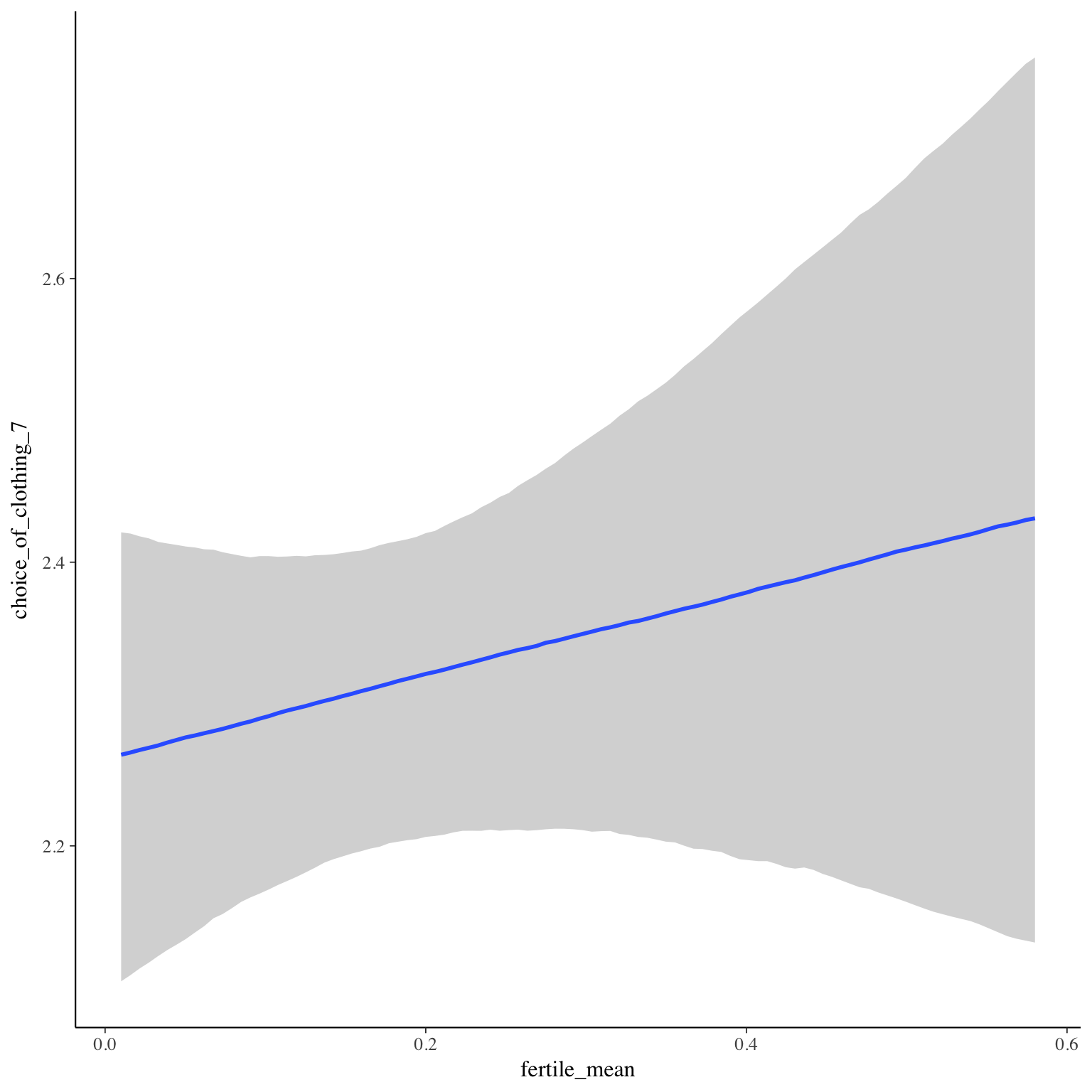
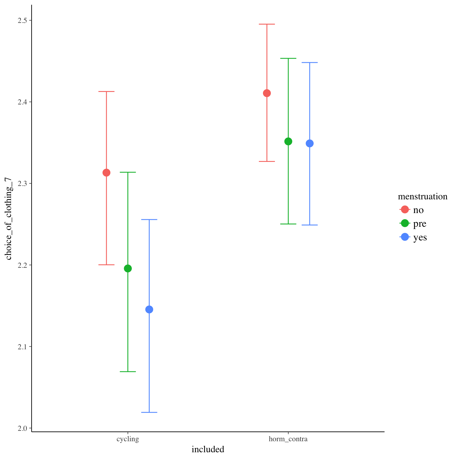
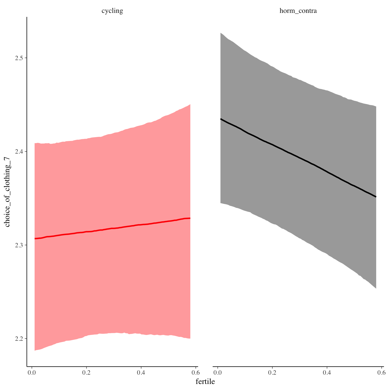
choice_of_clothing_7
Item text:
Verführerisch
Item translation:
22. seductive
Choices:
| choice | value | frequency | percent |
|---|---|---|---|
| 1 | Stimme nicht zu | 10425 | 0.35 |
| 2 | Stimme überwiegend nicht zu | 4983 | 0.17 |
| 3 | Stimme eher nicht zu | 7017 | 0.23 |
| 4 | Stimme eher zu | 4902 | 0.16 |
| 5 | Stimme überwiegend zu | 2004 | 0.07 |
| 6 | Stimme voll zu | 550 | 0.02 |
Model
Model summary
Family: cumulative(logit)
Formula: choice_of_clothing_7 ~ included * (menstruation + fertile) + fertile_mean + (1 + fertile + menstruation | person)
disc = 1
Data: diary (Number of observations: 26548)
Samples: 4 chains, each with iter = 2000; warmup = 1000; thin = 1;
total post-warmup samples = 4000
ICs: LOO = 70438.85; WAIC = Not computed
Group-Level Effects:
~person (Number of levels: 1043)
Estimate Est.Error l-95% CI u-95% CI Eff.Sample Rhat
sd(Intercept) 1.68 0.05 1.58 1.78 569 1.00
sd(fertile) 1.34 0.13 1.08 1.58 374 1.01
sd(menstruationpre) 0.25 0.13 0.02 0.47 71 1.05
sd(menstruationyes) 0.39 0.12 0.10 0.58 89 1.05
cor(Intercept,fertile) -0.18 0.08 -0.33 -0.02 1768 1.00
cor(Intercept,menstruationpre) 0.19 0.25 -0.29 0.73 398 1.00
cor(fertile,menstruationpre) -0.10 0.31 -0.78 0.45 207 1.02
cor(Intercept,menstruationyes) -0.05 0.15 -0.32 0.27 1139 1.00
cor(fertile,menstruationyes) 0.06 0.22 -0.48 0.40 225 1.04
cor(menstruationpre,menstruationyes) 0.29 0.42 -0.76 0.87 51 1.11
Population-Level Effects:
Estimate Est.Error l-95% CI u-95% CI Eff.Sample Rhat
Intercept[1] -0.68 0.13 -0.94 -0.41 424 1.01
Intercept[2] 0.36 0.13 0.10 0.64 429 1.01
Intercept[3] 1.81 0.13 1.55 2.08 440 1.01
Intercept[4] 3.38 0.14 3.13 3.66 453 1.01
Intercept[5] 5.21 0.14 4.94 5.50 484 1.01
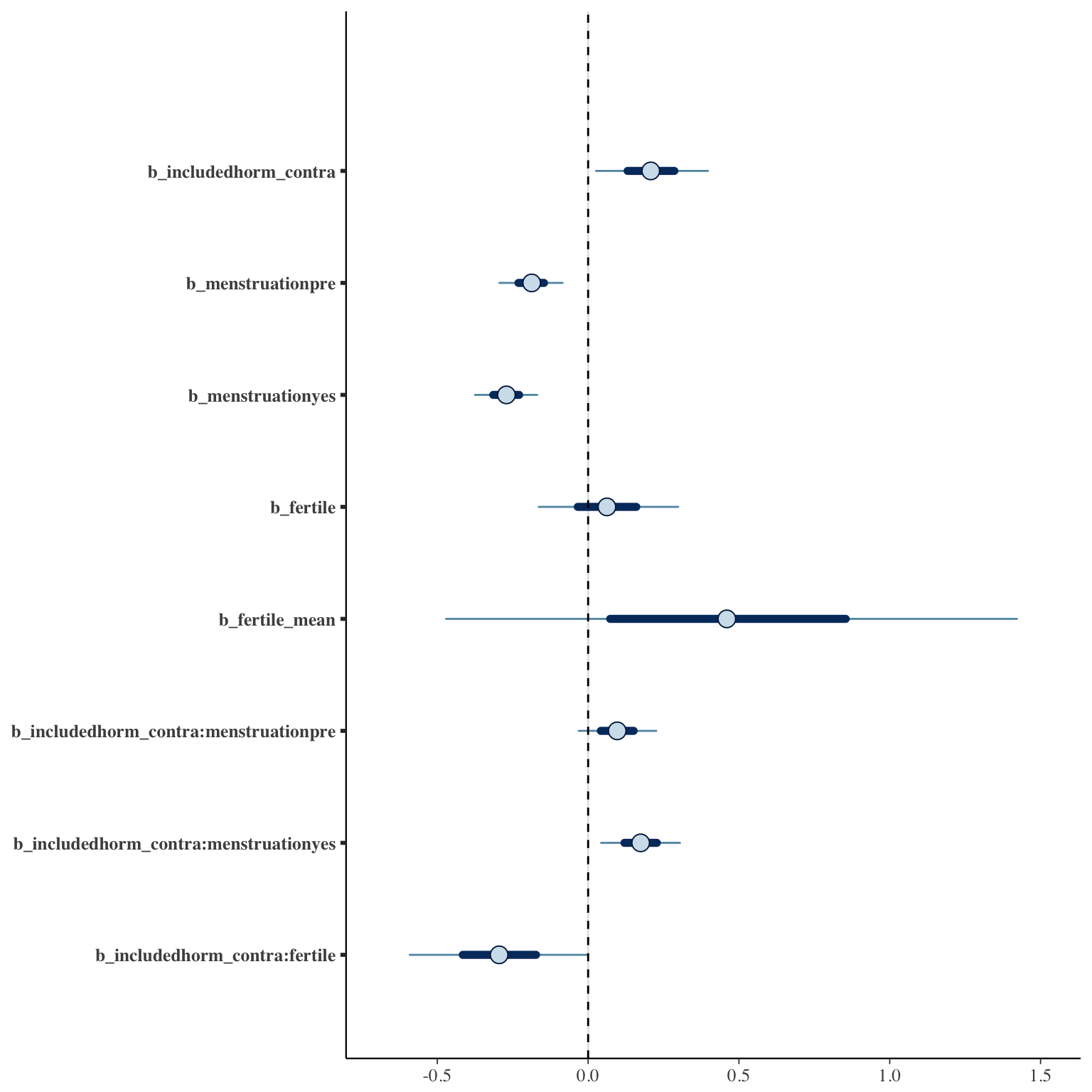
includedhorm_contra 0.21 0.11 -0.01 0.44 334 1.02
menstruationpre -0.19 0.06 -0.31 -0.07 1762 1.00
menstruationyes -0.27 0.06 -0.40 -0.15 1953 1.00
fertile 0.06 0.14 -0.20 0.35 1677 1.00
fertile_mean 0.47 0.57 -0.65 1.62 810 1.01
includedhorm_contra:menstruationpre 0.10 0.08 -0.06 0.25 1853 1.00
includedhorm_contra:menstruationyes 0.17 0.08 0.02 0.33 2039 1.00
includedhorm_contra:fertile -0.30 0.18 -0.64 0.05 1762 1.00
Samples were drawn using sampling(NUTS). For each parameter, Eff.Sample
is a crude measure of effective sample size, and Rhat is the potential
scale reduction factor on split chains (at convergence, Rhat = 1).
Coefficient plot
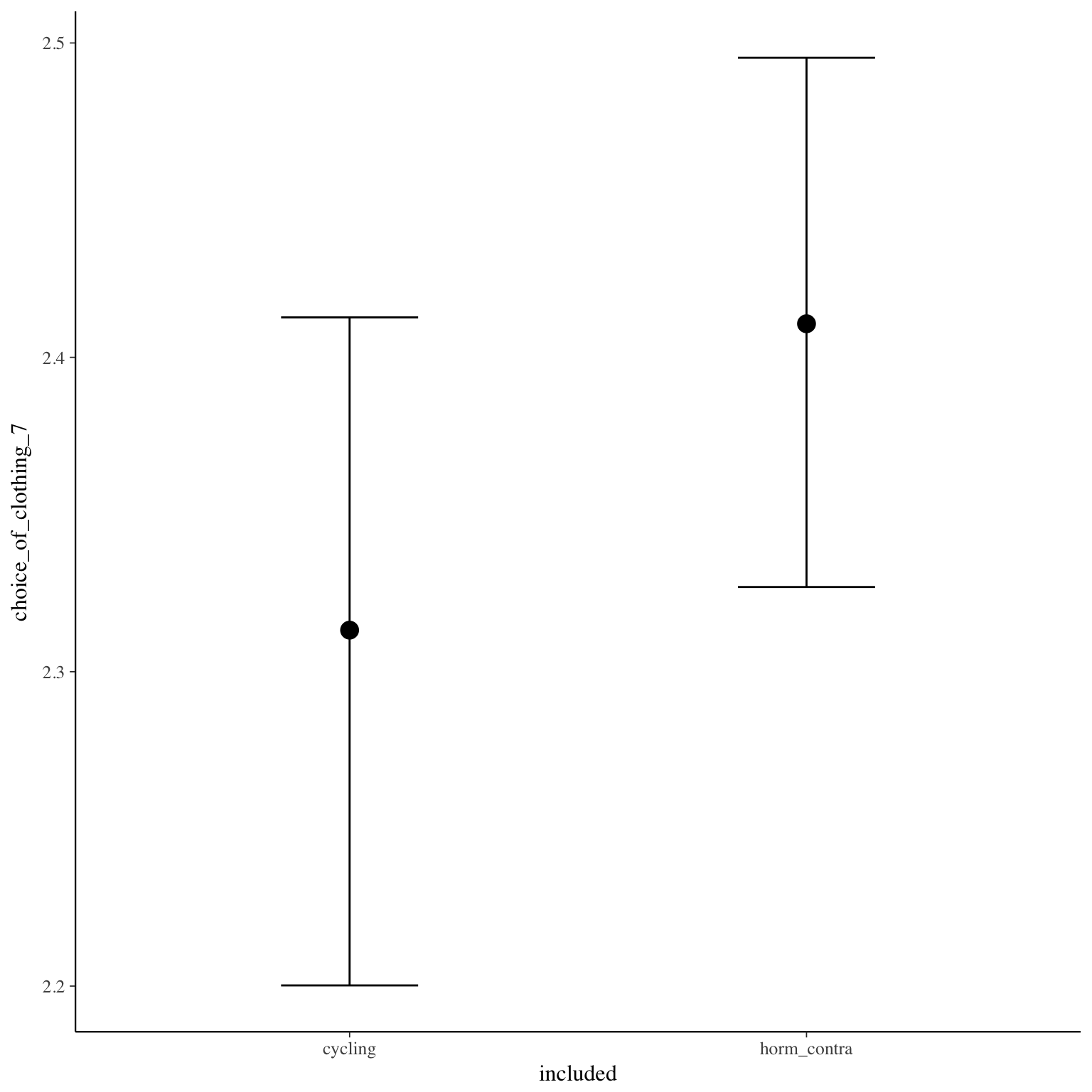
Marginal effect plots
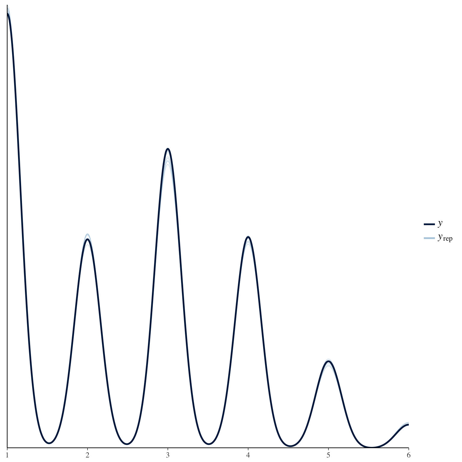
Diagnostics
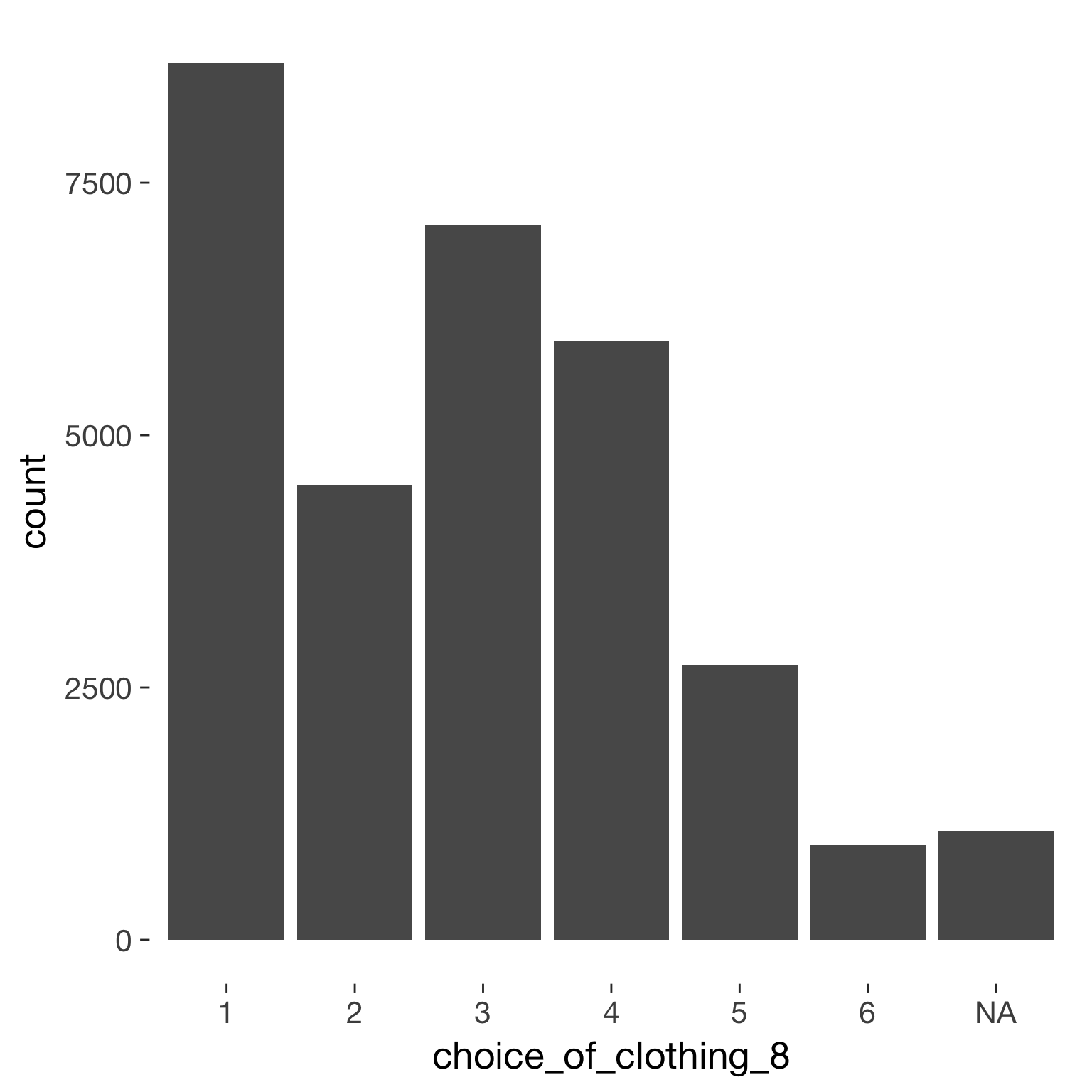
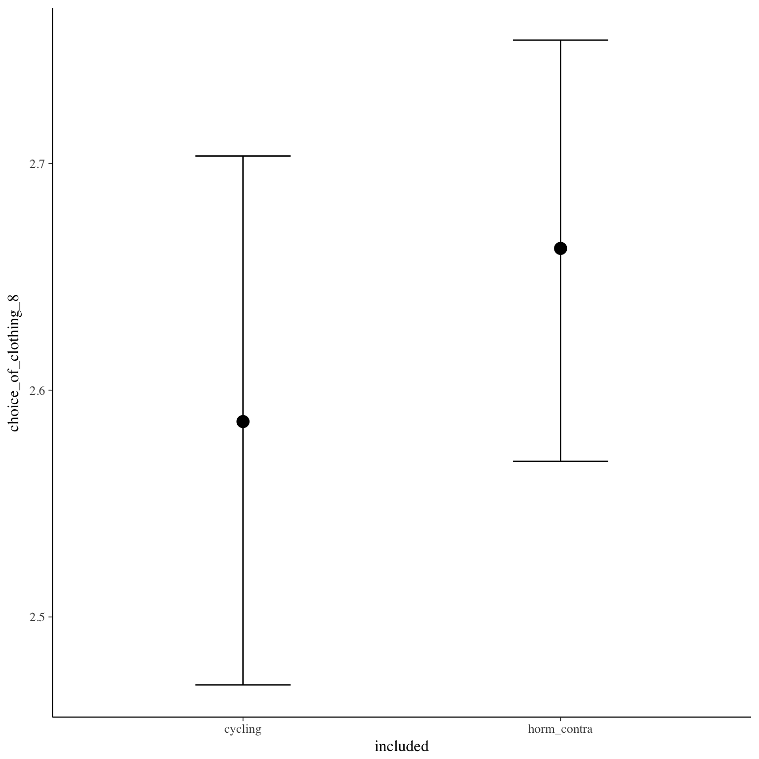
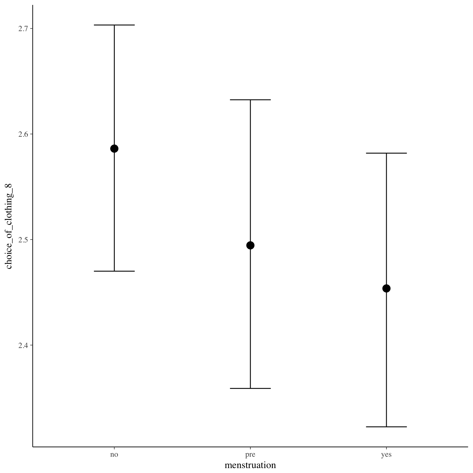
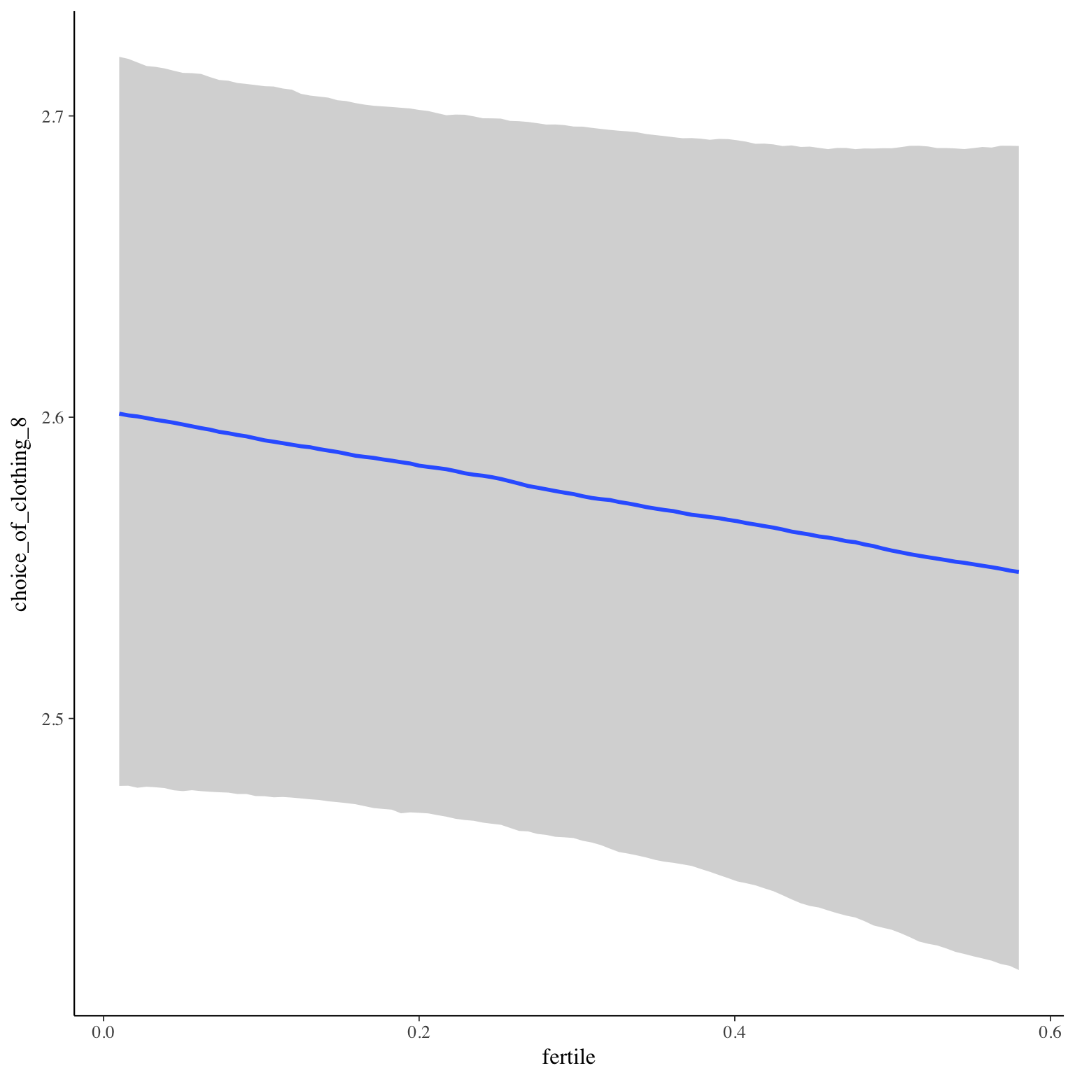
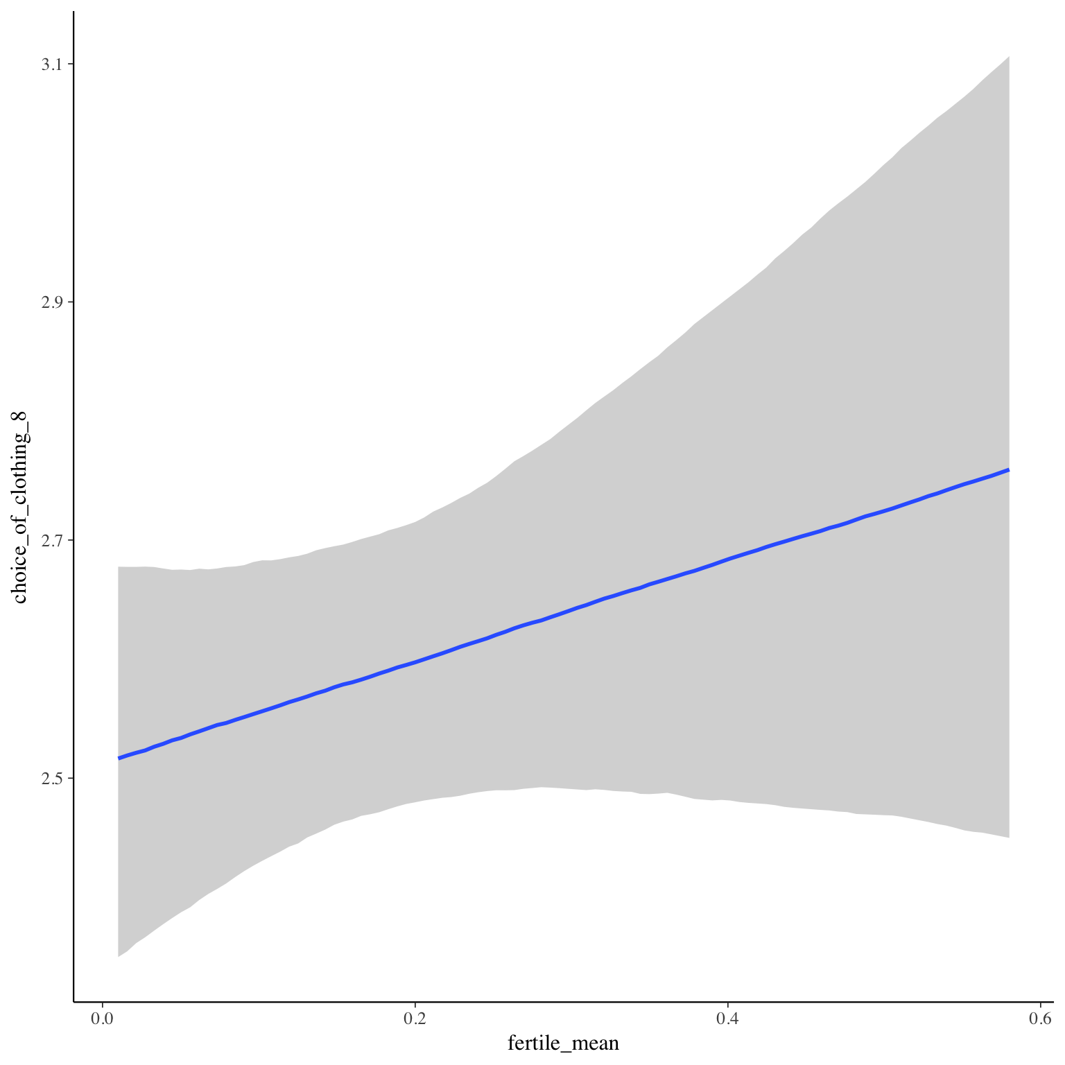
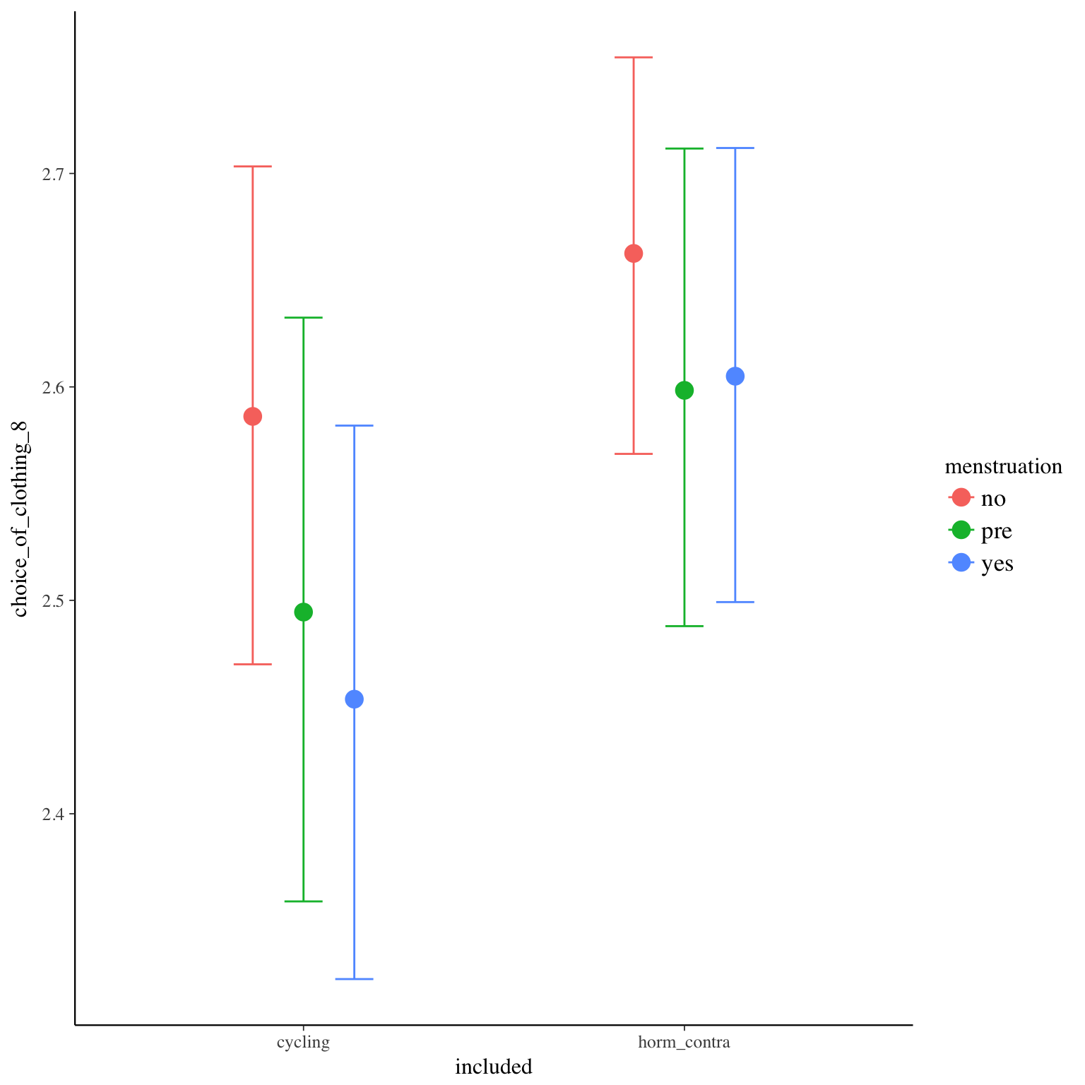
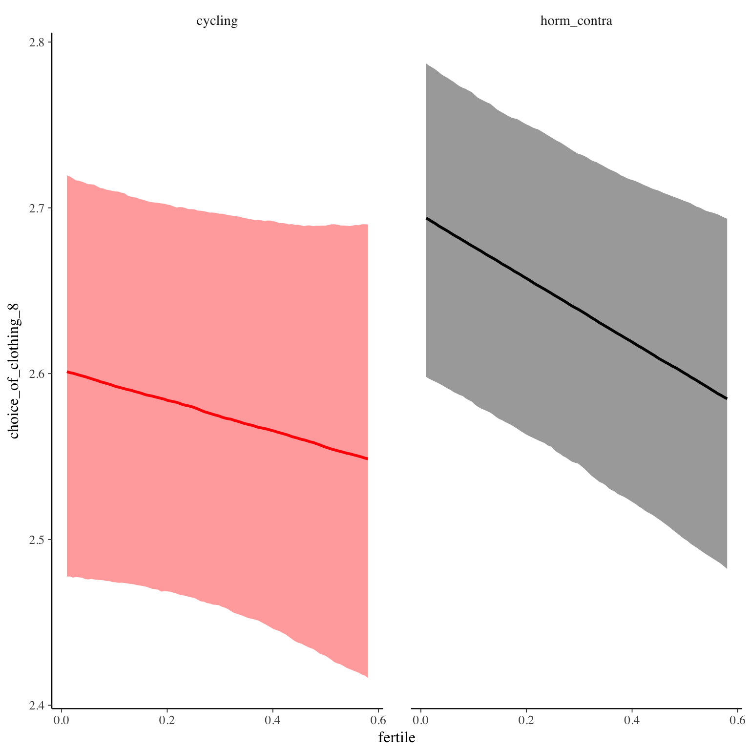
choice_of_clothing_8
Item text:
Auffällig
Item translation:
23. noticeable
Choices:
| choice | value | frequency | percent |
|---|---|---|---|
| 1 | Stimme nicht zu | 8689 | 0.29 |
| 2 | Stimme überwiegend nicht zu | 4507 | 0.15 |
| 3 | Stimme eher nicht zu | 7087 | 0.24 |
| 4 | Stimme eher zu | 5938 | 0.2 |
| 5 | Stimme überwiegend zu | 2720 | 0.09 |
| 6 | Stimme voll zu | 941 | 0.03 |
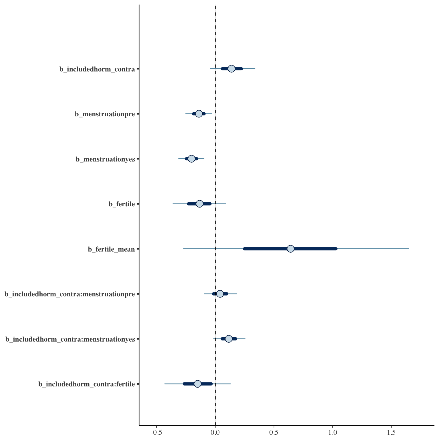
Model
Model summary
 Family: cumulative(logit)
Formula: choice_of_clothing_8 ~ included * (menstruation + fertile) + fertile_mean + (1 + fertile + menstruation | person)
         disc = 1
   Data: diary (Number of observations: 26549)
Samples: 4 chains, each with iter = 2000; warmup = 1000; thin = 1;
         total post-warmup samples = 4000
    ICs: LOO = 73271.26; WAIC = Not computed

Group-Level Effects:
~person (Number of levels: 1043)
                                     Estimate Est.Error l-95% CI u-95% CI Eff.Sample Rhat
sd(Intercept)                            1.68      0.05     1.58     1.77        805 1.00
sd(fertile)                              1.04      0.14     0.76     1.31        296 1.02
sd(menstruationpre)                      0.41      0.10     0.19     0.58         77 1.03
sd(menstruationyes)                      0.49      0.07     0.34     0.63        319 1.02
cor(Intercept,fertile)                   0.01      0.10    -0.18     0.22        894 1.00
cor(Intercept,menstruationpre)           0.21      0.15    -0.05     0.55        215 1.01
cor(fertile,menstruationpre)             0.05      0.26    -0.55     0.46        134 1.02
cor(Intercept,menstruationyes)          -0.07      0.10    -0.26     0.13       1768 1.00
cor(fertile,menstruationyes)             0.02      0.20    -0.40     0.37        234 1.02
cor(menstruationpre,menstruationyes)     0.07      0.23    -0.45     0.46        120 1.03

Population-Level Effects:
                                    Estimate Est.Error l-95% CI u-95% CI Eff.Sample Rhat
Intercept[1]                           -1.09      0.13    -1.35    -0.82        556 1.00
Intercept[2]                           -0.06      0.13    -0.32     0.21        565 1.00
Intercept[3]                            1.35      0.13     1.09     1.63        561 1.01
Intercept[4]                            2.96      0.14     2.69     3.23        574 1.01
Intercept[5]                            4.72      0.14     4.45     4.99        627 1.01
includedhorm_contra                     0.14      0.12    -0.08     0.38        339 1.01
menstruationpre                        -0.14      0.07    -0.27    -0.01       2265 1.00
menstruationyes                        -0.20      0.07    -0.33    -0.07       2303 1.00
fertile                                -0.14      0.14    -0.40     0.13       2201 1.00
fertile_mean                            0.65      0.58    -0.43     1.83        846 1.00
includedhorm_contra:menstruationpre     0.04      0.08    -0.12     0.22       2427 1.00
includedhorm_contra:menstruationyes     0.12      0.08    -0.04     0.28       2668 1.00
includedhorm_contra:fertile            -0.15      0.17    -0.47     0.18       2133 1.00

Samples were drawn using sampling(NUTS). For each parameter, Eff.Sample
is a crude measure of effective sample size, and Rhat is the potential
scale reduction factor on split chains (at convergence, Rhat = 1).
Coefficient plot
Marginal effect plots
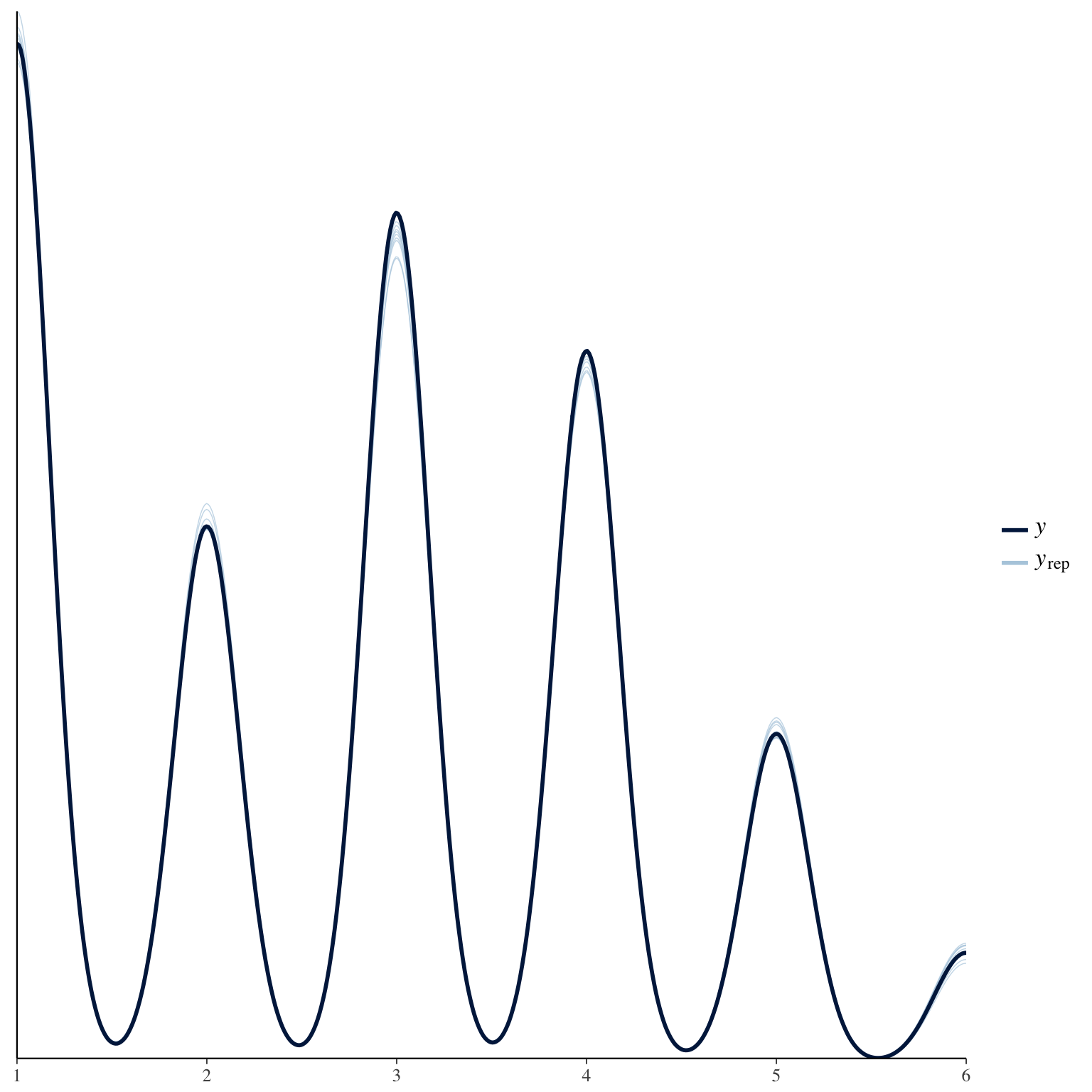
Diagnostics
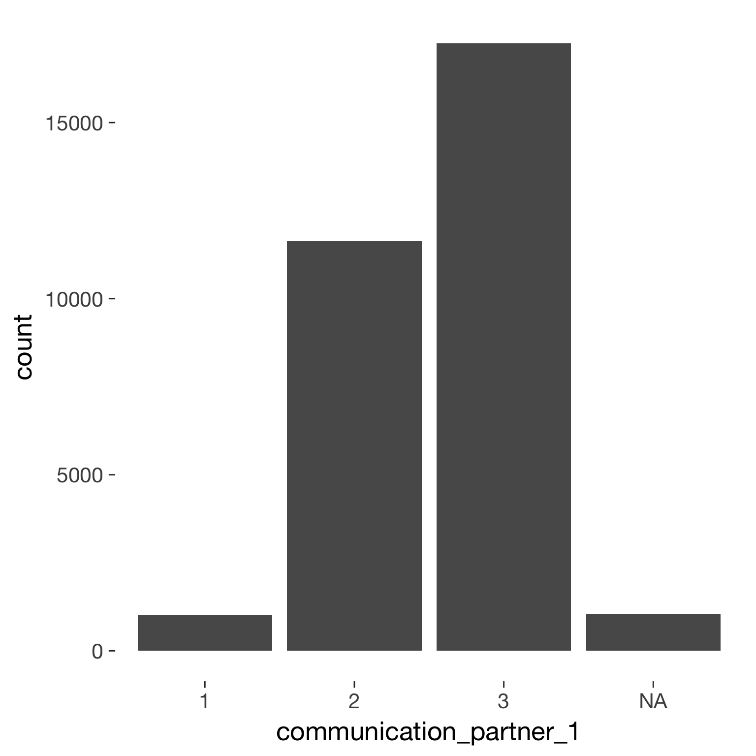
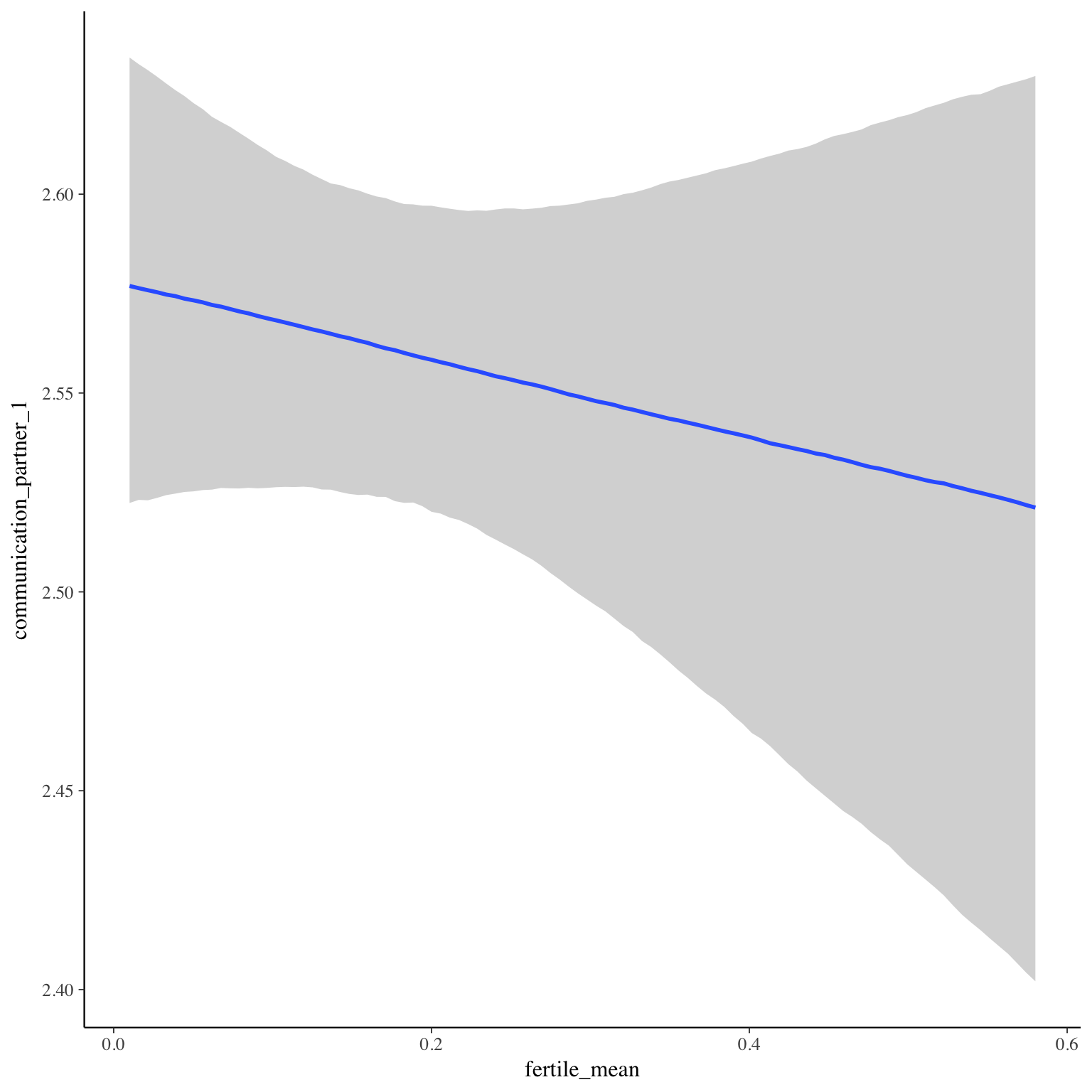
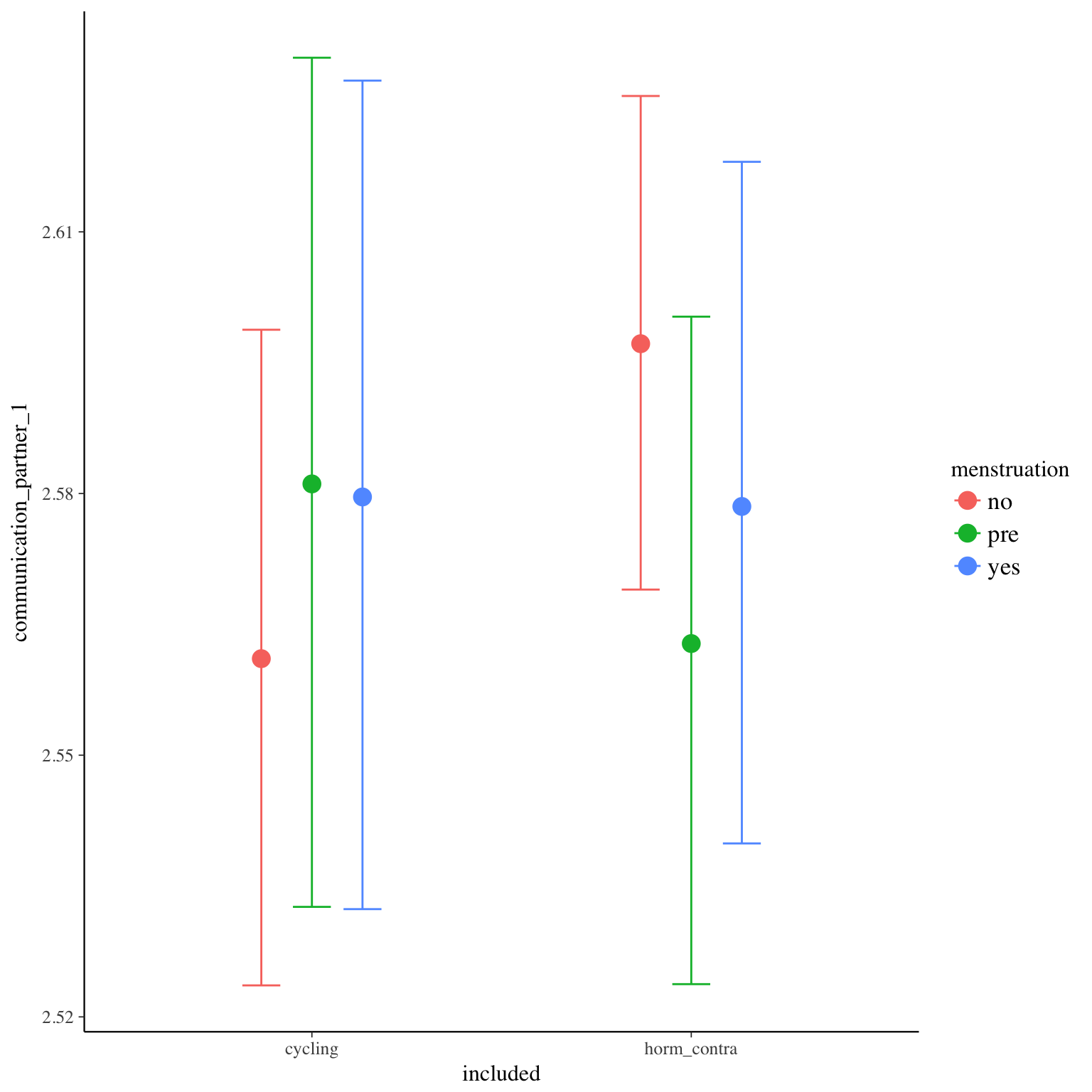
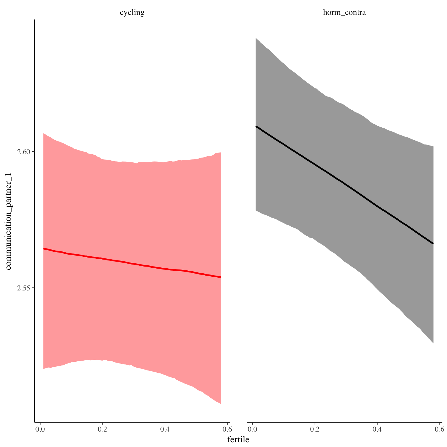
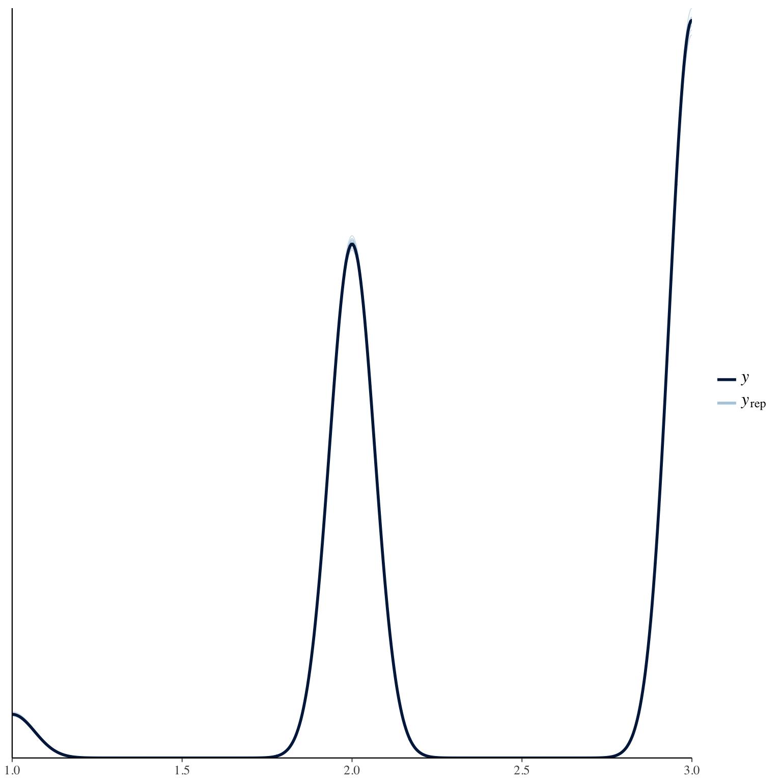
communication_partner_1
Item text:
Wie oft haben Sie seit Ihrem letzten Eintrag mit Ihrem Partner kommuniziert?
Item translation:
1. How often did you communicate with your partner?
Choices:
| choice | value | frequency | percent |
|---|---|---|---|
| 1 | Gar nicht | 1027 | 0.03 |
| 2 | Wenig | 11628 | 0.39 |
| 3 | Viel | 17247 | 0.58 |
Model
Model summary
 Family: cumulative(logit)
Formula: communication_partner_1 ~ included * (menstruation + fertile) + fertile_mean + (1 + fertile + menstruation | person)
         disc = 1
   Data: diary (Number of observations: 26568)
Samples: 4 chains, each with iter = 2000; warmup = 1000; thin = 1;
         total post-warmup samples = 4000
    ICs: LOO = 37037.95; WAIC = Not computed

Group-Level Effects:
~person (Number of levels: 1043)
                                     Estimate Est.Error l-95% CI u-95% CI Eff.Sample Rhat
sd(Intercept)                            1.32      0.05     1.22     1.42       1344 1.00
sd(fertile)                              1.81      0.13     1.54     2.08        556 1.01
sd(menstruationpre)                      0.82      0.07     0.69     0.96        852 1.00
sd(menstruationyes)                      0.75      0.07     0.60     0.89        989 1.00
cor(Intercept,fertile)                  -0.37      0.07    -0.49    -0.24       1702 1.00
cor(Intercept,menstruationpre)          -0.34      0.08    -0.48    -0.19       1822 1.00
cor(fertile,menstruationpre)             0.45      0.09     0.27     0.61        574 1.01
cor(Intercept,menstruationyes)          -0.17      0.09    -0.33     0.01       1787 1.00
cor(fertile,menstruationyes)             0.56      0.09     0.38     0.73        802 1.00
cor(menstruationpre,menstruationyes)     0.51      0.10     0.30     0.69        754 1.00

Population-Level Effects:
                                    Estimate Est.Error l-95% CI u-95% CI Eff.Sample Rhat
Intercept[1]                           -4.07      0.12    -4.32    -3.83       1364    1
Intercept[2]                           -0.40      0.12    -0.65    -0.17       1283    1
includedhorm_contra                     0.18      0.10    -0.02     0.38       1061    1
menstruationpre                         0.08      0.08    -0.09     0.24       2087    1
menstruationyes                         0.07      0.08    -0.08     0.22       2136    1
fertile                                -0.07      0.17    -0.41     0.26       1857    1
fertile_mean                           -0.37      0.50    -1.38     0.60       2277    1
includedhorm_contra:menstruationpre    -0.21      0.11    -0.43    -0.01       1869    1
includedhorm_contra:menstruationyes    -0.14      0.10    -0.34     0.05       2106    1
includedhorm_contra:fertile            -0.23      0.21    -0.62     0.17       1746    1

Samples were drawn using sampling(NUTS). For each parameter, Eff.Sample
is a crude measure of effective sample size, and Rhat is the potential
scale reduction factor on split chains (at convergence, Rhat = 1).
Coefficient plot
Marginal effect plots
Diagnostics
communication_partner_2
Item text:
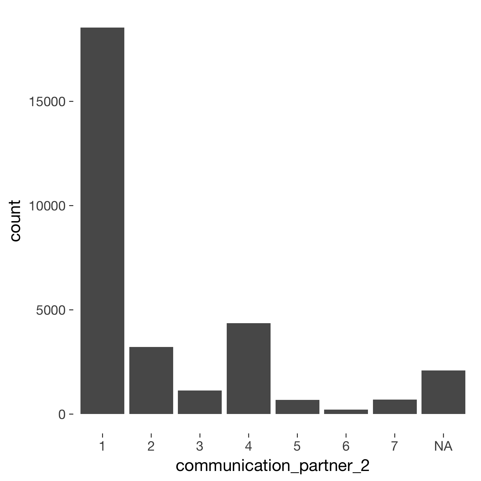
Auf welche Art haben Sie hauptsächlich mit Ihrem Partner kommuniziert?
Item translation:
2. How did you communicate mainly with your partner?
Choices:
| choice | value | frequency | percent |
|---|---|---|---|
| 1 | Direkter persönlicher Kontakt | 18537 | 0.64 |
| 2 | Telefon | 3226 | 0.11 |
| 3 | SMS | 1126 | 0.04 |
| 4 | mobile Nachrichtenapp (z.B. Whatsapp) | 4368 | 0.15 |
| 5 | Webcam (z.B. Skype) | 681 | 0.02 |
| 6 | 216 | 0.01 | |
| 7 | Chat (z.B. Facebook) | 703 | 0.02 |
Model
Model summary
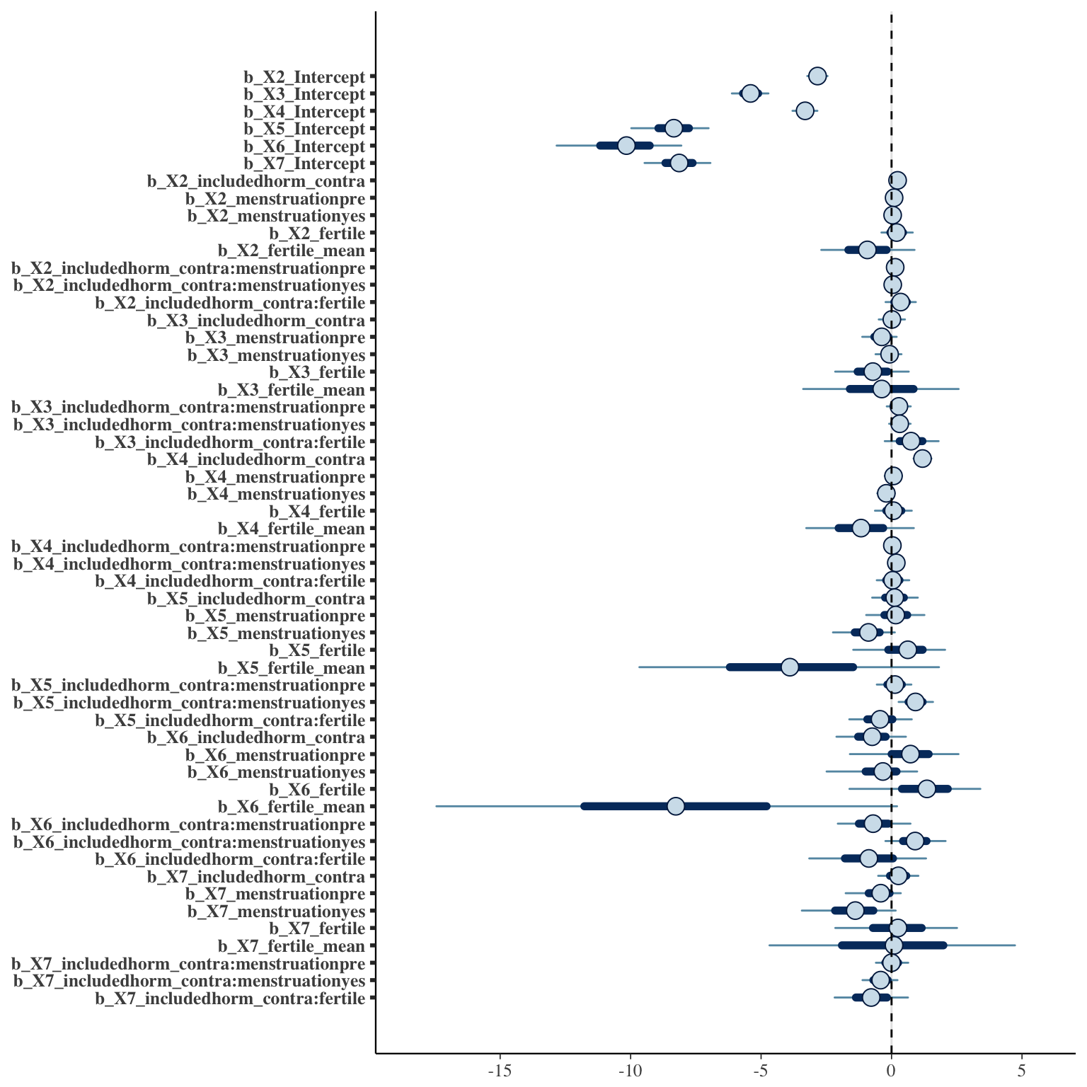
 Family: categorical(logit)
Formula: communication_partner_2 ~ included * (menstruation + fertile) + fertile_mean + (1 + fertile + menstruation | person)
   Data: diary (Number of observations: 25656)
Samples: 4 chains, each with iter = 2000; warmup = 1000; thin = 1;
         total post-warmup samples = 4000
    ICs: LOO = 38999.67; WAIC = Not computed

Group-Level Effects:
~person (Number of levels: 1039)
                                           Estimate Est.Error l-95% CI u-95% CI Eff.Sample Rhat
sd(X2_Intercept)                               2.06      0.10     1.87     2.28       1814 1.00
sd(X2_fertile)                                 1.95      0.25     1.45     2.45        552 1.00
sd(X2_menstruationpre)                         0.69      0.17     0.27     0.97        421 1.00
sd(X2_menstruationyes)                         0.52      0.22     0.05     0.92        268 1.02
sd(X3_Intercept)                               2.83      0.19     2.48     3.22       1374 1.00
sd(X3_fertile)                                 2.50      0.44     1.66     3.39        765 1.00
sd(X3_menstruationpre)                         0.78      0.31     0.12     1.37        409 1.01
sd(X3_menstruationyes)                         0.38      0.26     0.02     0.95        564 1.01
sd(X4_Intercept)                               2.46      0.12     2.23     2.69       1707 1.00
sd(X4_fertile)                                 1.86      0.25     1.36     2.34        739 1.01
sd(X4_menstruationpre)                         0.75      0.13     0.48     0.99        647 1.00
sd(X4_menstruationyes)                         0.84      0.14     0.56     1.12       1042 1.00
sd(X5_Intercept)                               4.86      0.41     4.11     5.74       1167 1.00
sd(X5_fertile)                                 1.00      0.66     0.04     2.43        722 1.00
sd(X5_menstruationpre)                         1.08      0.31     0.46     1.69        944 1.00
sd(X5_menstruationyes)                         0.93      0.37     0.16     1.67        987 1.00
sd(X6_Intercept)                               4.91      0.68     3.75     6.41       1039 1.00
sd(X6_fertile)                                 1.04      0.82     0.04     3.06       1371 1.00
sd(X6_menstruationpre)                         1.32      0.70     0.11     2.84        904 1.00
sd(X6_menstruationyes)                         0.81      0.57     0.05     2.16       1139 1.00
sd(X7_Intercept)                               3.97      0.36     3.33     4.75       1276 1.00
sd(X7_fertile)                                 3.00      0.56     1.93     4.14       1022 1.00
sd(X7_menstruationpre)                         0.56      0.36     0.03     1.35        648 1.00
sd(X7_menstruationyes)                         1.27      0.58     0.20     2.54       1426 1.00
cor(X2_Intercept,X2_fertile)                  -0.23      0.13    -0.47     0.04       2865 1.00
cor(X2_Intercept,X2_menstruationpre)          -0.18      0.18    -0.52     0.21       3209 1.00
cor(X2_fertile,X2_menstruationpre)             0.21      0.22    -0.33     0.57        509 1.00
cor(X2_Intercept,X2_menstruationyes)           0.05      0.25    -0.44     0.56       2384 1.00
cor(X2_fertile,X2_menstruationyes)             0.34      0.27    -0.31     0.79        858 1.00
cor(X2_menstruationpre,X2_menstruationyes)     0.23      0.33    -0.59     0.75        555 1.00
cor(X3_Intercept,X3_fertile)                  -0.01      0.19    -0.38     0.36       4000 1.00
cor(X3_Intercept,X3_menstruationpre)           0.16      0.28    -0.42     0.69       4000 1.00
cor(X3_fertile,X3_menstruationpre)             0.16      0.30    -0.54     0.68        939 1.00
cor(X3_Intercept,X3_menstruationyes)           0.05      0.39    -0.72     0.76       4000 1.00
cor(X3_fertile,X3_menstruationyes)             0.18      0.40    -0.68     0.82       1589 1.00
cor(X3_menstruationpre,X3_menstruationyes)     0.27      0.42    -0.67     0.90       1086 1.00
cor(X4_Intercept,X4_fertile)                  -0.01      0.15    -0.31     0.29       4000 1.00
cor(X4_Intercept,X4_menstruationpre)          -0.04      0.18    -0.39     0.32       4000 1.00
cor(X4_fertile,X4_menstruationpre)             0.37      0.17    -0.02     0.66        703 1.00
cor(X4_Intercept,X4_menstruationyes)           0.29      0.16    -0.04     0.59       2143 1.00
cor(X4_fertile,X4_menstruationyes)            -0.02      0.19    -0.42     0.31        592 1.01
cor(X4_menstruationpre,X4_menstruationyes)     0.43      0.17     0.07     0.75        764 1.00
cor(X5_Intercept,X5_fertile)                   0.16      0.42    -0.71     0.86       4000 1.00
cor(X5_Intercept,X5_menstruationpre)          -0.21      0.31    -0.76     0.41       4000 1.00
cor(X5_fertile,X5_menstruationpre)            -0.09      0.40    -0.81     0.69        488 1.00
cor(X5_Intercept,X5_menstruationyes)           0.21      0.33    -0.49     0.76       4000 1.00
cor(X5_fertile,X5_menstruationyes)             0.06      0.42    -0.76     0.80        600 1.01
cor(X5_menstruationpre,X5_menstruationyes)     0.35      0.32    -0.38     0.85       1679 1.00
cor(X6_Intercept,X6_fertile)                   0.07      0.44    -0.78     0.82       4000 1.00
cor(X6_Intercept,X6_menstruationpre)          -0.24      0.37    -0.84     0.53       4000 1.00
cor(X6_fertile,X6_menstruationpre)             0.07      0.44    -0.76     0.84       1155 1.00
cor(X6_Intercept,X6_menstruationyes)           0.05      0.42    -0.77     0.78       4000 1.00
cor(X6_fertile,X6_menstruationyes)             0.10      0.45    -0.78     0.85       2282 1.00
cor(X6_menstruationpre,X6_menstruationyes)     0.05      0.43    -0.76     0.80       3070 1.00
cor(X7_Intercept,X7_fertile)                  -0.04      0.24    -0.51     0.43       2886 1.00
cor(X7_Intercept,X7_menstruationpre)           0.25      0.41    -0.65     0.87       4000 1.00
cor(X7_fertile,X7_menstruationpre)            -0.20      0.37    -0.83     0.57       2658 1.00
cor(X7_Intercept,X7_menstruationyes)           0.68      0.25     0.00     0.95       1853 1.00
cor(X7_fertile,X7_menstruationyes)             0.17      0.27    -0.40     0.65       1972 1.00
cor(X7_menstruationpre,X7_menstruationyes)     0.15      0.41    -0.73     0.81       1704 1.00

Population-Level Effects:
                                       Estimate Est.Error l-95% CI u-95% CI Eff.Sample Rhat
X2_Intercept                              -2.84      0.24    -3.31    -2.38       1897    1
X3_Intercept                              -5.41      0.43    -6.25    -4.60       2297    1
X4_Intercept                              -3.31      0.28    -3.88    -2.77       1492    1
X5_Intercept                              -8.39      0.90   -10.26    -6.74       1317    1
X6_Intercept                             -10.27      1.43   -13.42    -7.72       1784    1
X7_Intercept                              -8.16      0.77    -9.74    -6.73       1873    1
X2_includedhorm_contra                     0.23      0.18    -0.14     0.57       1527    1
X2_menstruationpre                         0.10      0.17    -0.23     0.43       3175    1
X2_menstruationyes                         0.04      0.17    -0.29     0.34       1743    1
X2_fertile                                 0.20      0.36    -0.50     0.92       3066    1
X2_fertile_mean                           -0.92      1.08    -3.03     1.20       1827    1
X2_includedhorm_contra:menstruationpre     0.14      0.16    -0.19     0.47       4000    1
X2_includedhorm_contra:menstruationyes     0.05      0.16    -0.26     0.36       4000    1
X2_includedhorm_contra:fertile             0.35      0.35    -0.34     1.03       4000    1
X3_includedhorm_contra                     0.01      0.30    -0.59     0.61       1550    1
X3_menstruationpre                        -0.41      0.41    -1.27     0.30       2653    1
X3_menstruationyes                        -0.09      0.30    -0.73     0.48       4000    1
X3_fertile                                -0.74      0.86    -2.48     0.91       2808    1
X3_fertile_mean                           -0.39      1.82    -4.01     3.15       1965    1
X3_includedhorm_contra:menstruationpre     0.28      0.28    -0.28     0.81       4000    1
X3_includedhorm_contra:menstruationyes     0.31      0.25    -0.16     0.81       4000    1
X3_includedhorm_contra:fertile             0.75      0.63    -0.47     1.99       4000    1
X4_includedhorm_contra                     1.19      0.21     0.77     1.60       1116    1
X4_menstruationpre                         0.07      0.20    -0.32     0.46       2602    1
X4_menstruationyes                        -0.20      0.20    -0.61     0.19       3034    1
X4_fertile                                 0.08      0.42    -0.77     0.91       2698    1
X4_fertile_mean                           -1.18      1.26    -3.64     1.25       1534    1
X4_includedhorm_contra:menstruationpre     0.03      0.17    -0.32     0.37       4000    1
X4_includedhorm_contra:menstruationyes     0.18      0.18    -0.15     0.54       4000    1
X4_includedhorm_contra:fertile             0.05      0.37    -0.67     0.79       4000    1
X5_includedhorm_contra                     0.12      0.53    -0.91     1.13       1092    1
X5_menstruationpre                         0.16      0.68    -1.21     1.49       3310    1
X5_menstruationyes                        -0.96      0.73    -2.53     0.30       3148    1
X5_fertile                                 0.49      1.08    -2.03     2.39       2329    1
X5_fertile_mean                           -3.84      3.49   -10.76     3.01       1514    1
X5_includedhorm_contra:menstruationpre     0.12      0.41    -0.71     0.91       4000    1
X5_includedhorm_contra:menstruationyes     0.92      0.40     0.15     1.74       4000    1
X5_includedhorm_contra:fertile            -0.44      0.72    -1.87     0.97       4000    1
X6_includedhorm_contra                    -0.76      0.81    -2.40     0.80       1770    1
X6_menstruationpre                         0.66      1.26    -2.13     2.98       3225    1
X6_menstruationyes                        -0.48      1.09    -3.14     1.27       2166    1
X6_fertile                                 1.19      1.57    -2.49     3.81       2424    1
X6_fertile_mean                           -8.37      5.38   -19.34     1.82       2048    1
X6_includedhorm_contra:menstruationpre    -0.69      0.86    -2.37     0.98       4000    1
X6_includedhorm_contra:menstruationyes     0.91      0.70    -0.47     2.34       4000    1
X6_includedhorm_contra:fertile            -0.87      1.37    -3.60     1.77       4000    1
X7_includedhorm_contra                     0.26      0.47    -0.68     1.23       1417    1
X7_menstruationpre                        -0.53      0.65    -2.13     0.49       2032    1
X7_menstruationyes                        -1.48      1.10    -3.94     0.37       2086    1
X7_fertile                                 0.21      1.42    -2.73     2.92       2871    1
X7_fertile_mean                            0.05      2.89    -5.72     5.69       1757    1
X7_includedhorm_contra:menstruationpre     0.01      0.37    -0.72     0.79       4000    1
X7_includedhorm_contra:menstruationyes    -0.43      0.41    -1.25     0.34       4000    1
X7_includedhorm_contra:fertile            -0.77      0.87    -2.46     0.94       4000    1

Samples were drawn using sampling(NUTS). For each parameter, Eff.Sample
is a crude measure of effective sample size, and Rhat is the potential
scale reduction factor on split chains (at convergence, Rhat = 1).
Coefficient plot
Marginal effect plots
Error: Error: Marginal plots are not yet implemented for categorical models.
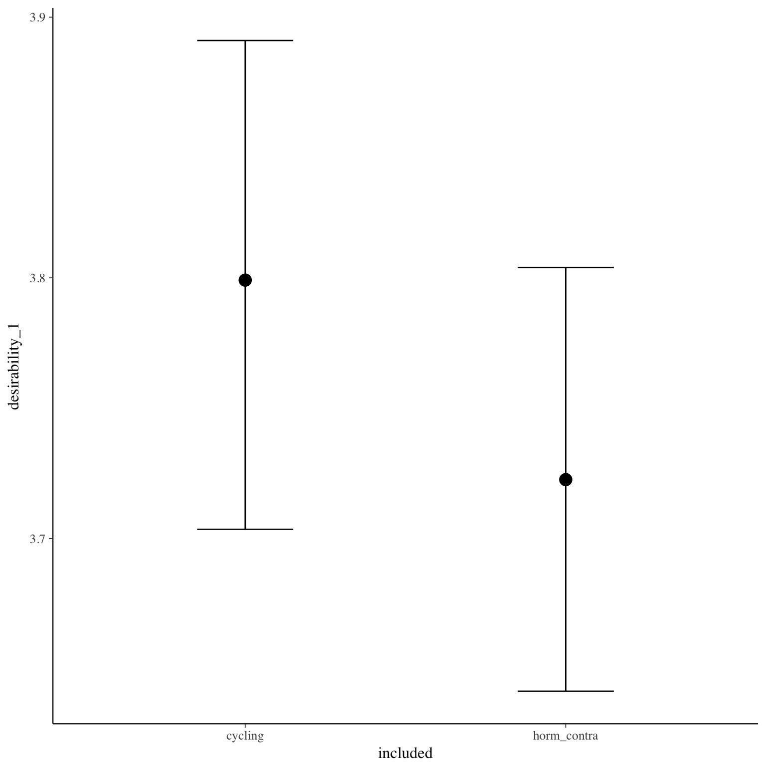
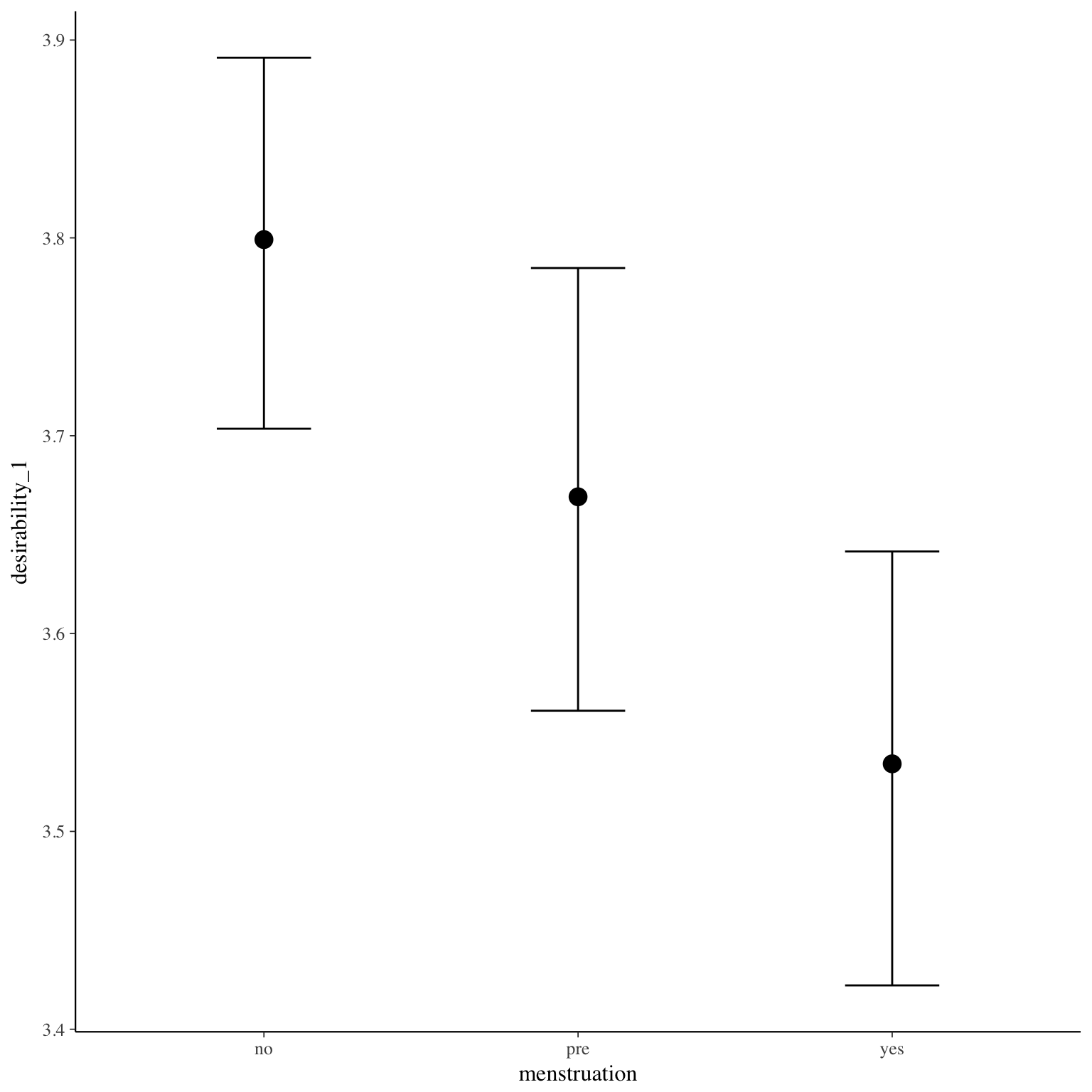
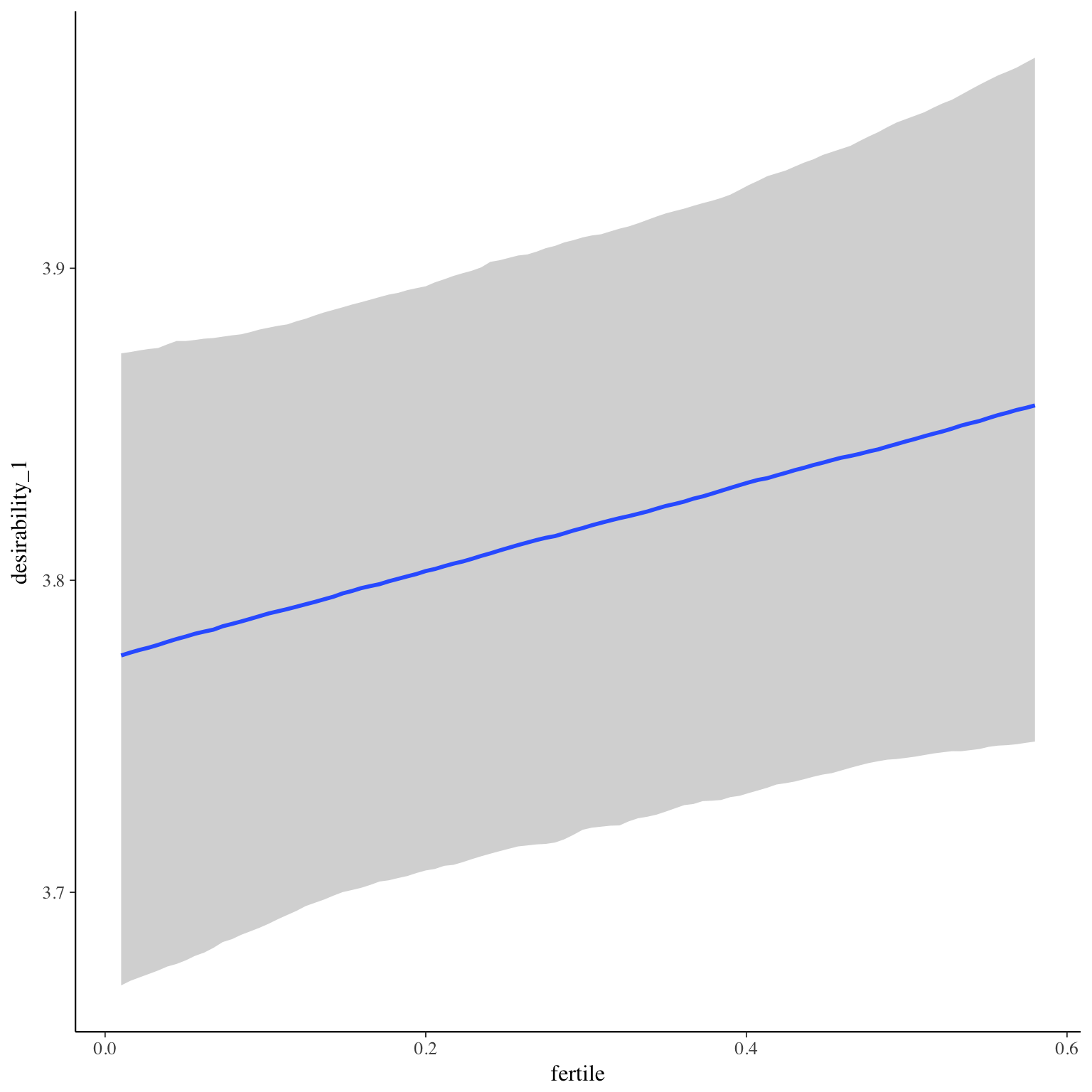
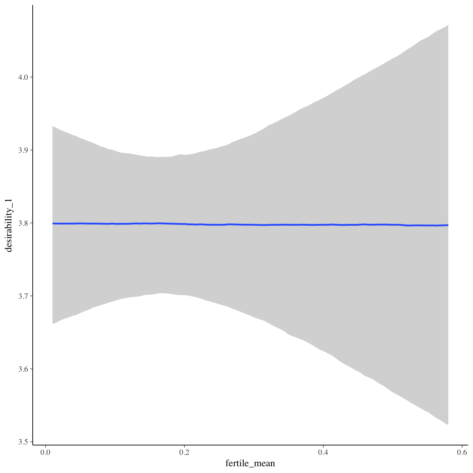
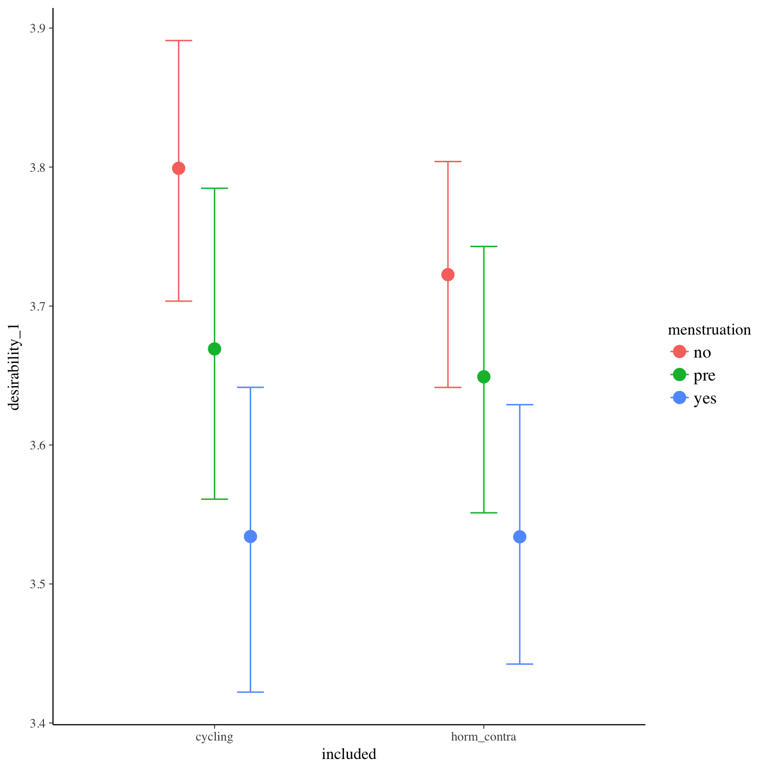
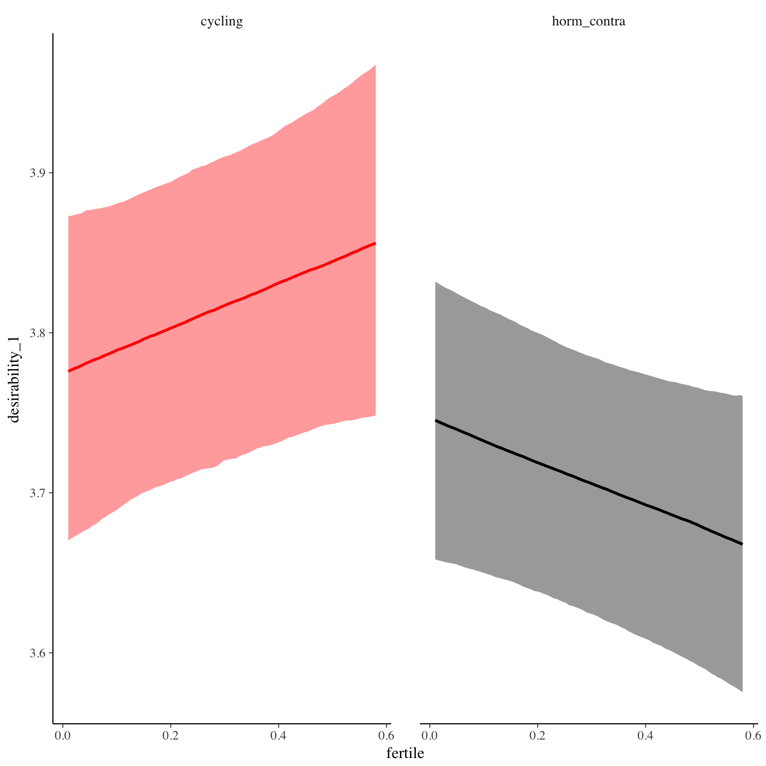
desirability_1
Item text:
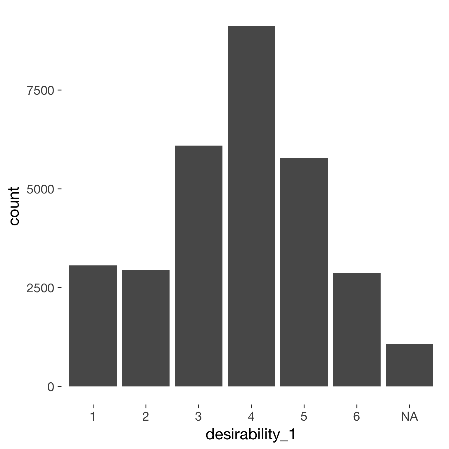
… habe ich mich sexuell begehrenswert gefühlt.
Item translation:
25. I felt sexually desirable.
Choices:
| choice | value | frequency | percent |
|---|---|---|---|
| 1 | Stimme nicht zu | 3063 | 0.1 |
| 2 | Stimme überwiegend nicht zu | 2944 | 0.1 |
| 3 | Stimme eher nicht zu | 6093 | 0.2 |
| 4 | Stimme eher zu | 9126 | 0.31 |
| 5 | Stimme überwiegend zu | 5787 | 0.19 |
| 6 | Stimme voll zu | 2868 | 0.1 |
Model
Model summary
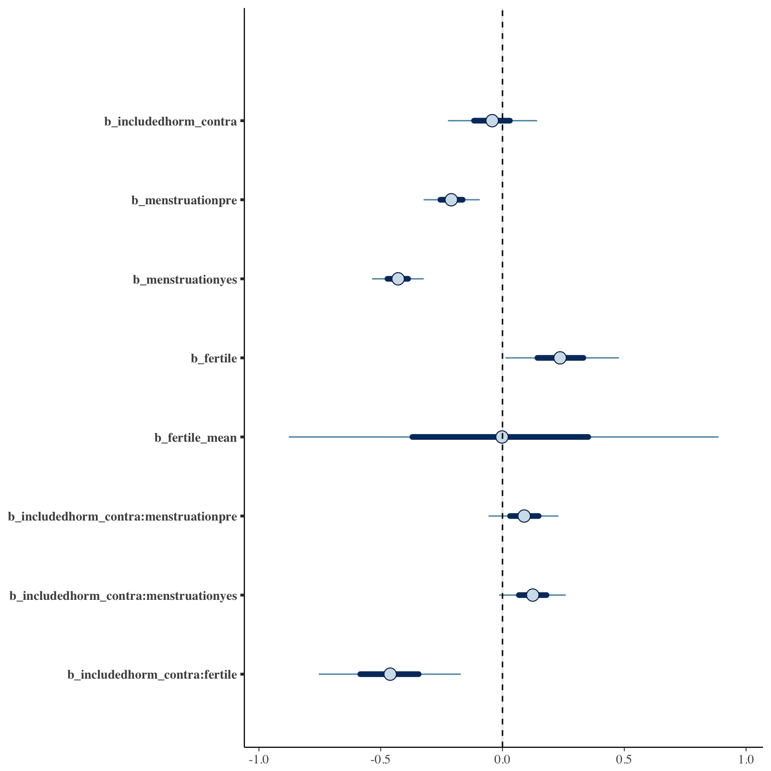
 Family: cumulative(logit)
Formula: desirability_1 ~ included * (menstruation + fertile) + fertile_mean + (1 + fertile + menstruation | person)
         disc = 1
   Data: diary (Number of observations: 26549)
Samples: 4 chains, each with iter = 2000; warmup = 1000; thin = 1;
         total post-warmup samples = 4000
    ICs: LOO = 77829.21; WAIC = Not computed

Group-Level Effects:
~person (Number of levels: 1043)
                                     Estimate Est.Error l-95% CI u-95% CI Eff.Sample Rhat
sd(Intercept)                            1.60      0.05     1.51     1.69        938 1.01
sd(fertile)                              1.52      0.12     1.29     1.74        704 1.00
sd(menstruationpre)                      0.65      0.06     0.54     0.77        730 1.01
sd(menstruationyes)                      0.66      0.06     0.54     0.77        728 1.01
cor(Intercept,fertile)                  -0.29      0.06    -0.41    -0.16       1909 1.00
cor(Intercept,menstruationpre)          -0.15      0.08    -0.29     0.01       1762 1.00
cor(fertile,menstruationpre)             0.34      0.10     0.12     0.51        708 1.00
cor(Intercept,menstruationyes)          -0.25      0.07    -0.38    -0.11       2404 1.00
cor(fertile,menstruationyes)             0.17      0.11    -0.06     0.37        650 1.00
cor(menstruationpre,menstruationyes)     0.37      0.10     0.15     0.56        548 1.02

Population-Level Effects:
                                    Estimate Est.Error l-95% CI u-95% CI Eff.Sample Rhat
Intercept[1]                           -3.07      0.13    -3.31    -2.83        904 1.01
Intercept[2]                           -1.99      0.12    -2.23    -1.75        886 1.01
Intercept[3]                           -0.60      0.12    -0.84    -0.36        871 1.01
Intercept[4]                            1.16      0.12     0.92     1.40        775 1.01
Intercept[5]                            2.89      0.13     2.66     3.14        784 1.01
includedhorm_contra                    -0.04      0.11    -0.26     0.17        645 1.00
menstruationpre                        -0.21      0.07    -0.34    -0.07       2230 1.00
menstruationyes                        -0.43      0.06    -0.55    -0.30       2054 1.00
fertile                                 0.24      0.14    -0.03     0.52       1971 1.00
fertile_mean                            0.00      0.53    -1.01     1.05       1254 1.00
includedhorm_contra:menstruationpre     0.09      0.09    -0.08     0.25       2164 1.00
includedhorm_contra:menstruationyes     0.12      0.08    -0.04     0.28       2045 1.00
includedhorm_contra:fertile            -0.46      0.18    -0.80    -0.11       1877 1.00

Samples were drawn using sampling(NUTS). For each parameter, Eff.Sample
is a crude measure of effective sample size, and Rhat is the potential
scale reduction factor on split chains (at convergence, Rhat = 1).
Coefficient plot
Marginal effect plots
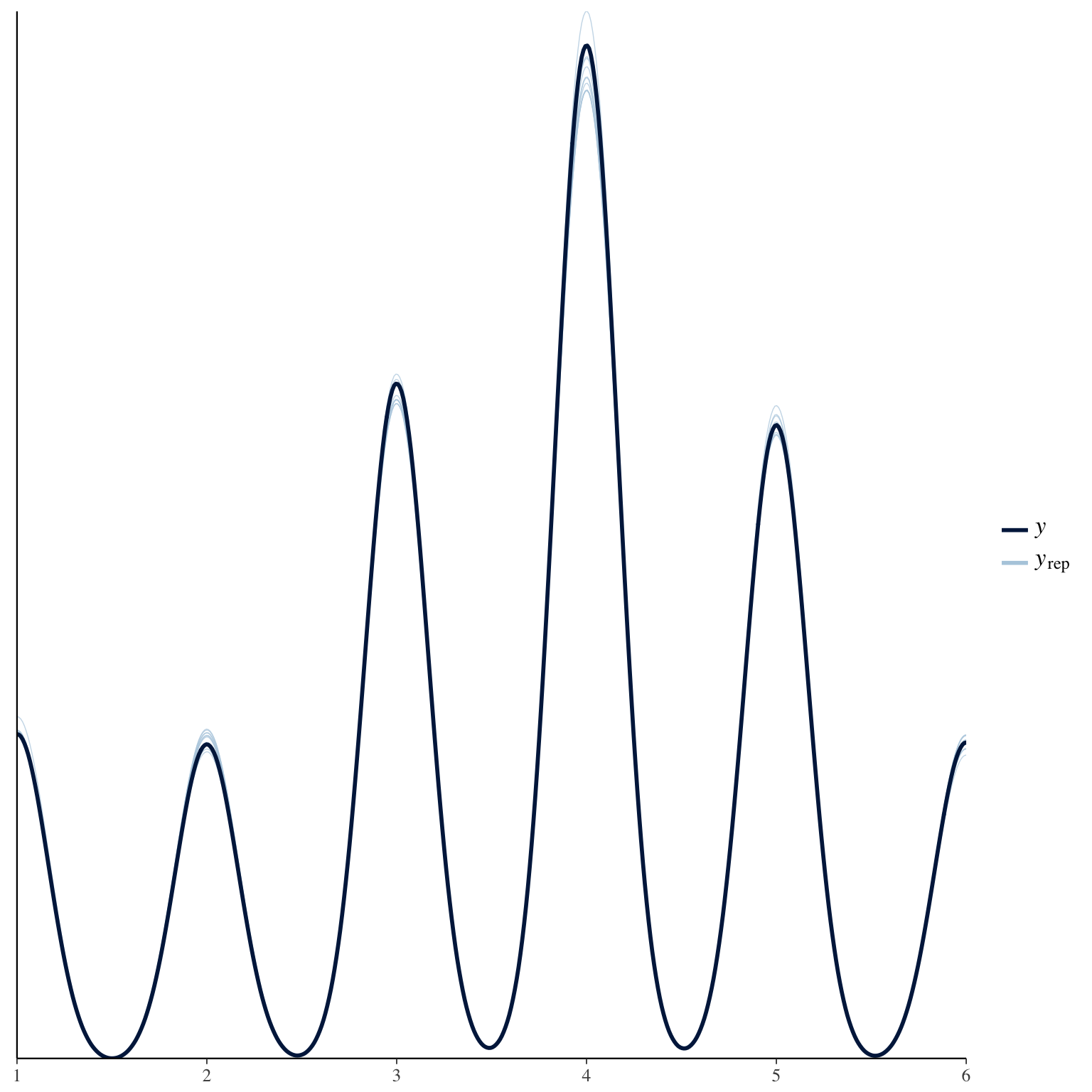
Diagnostics
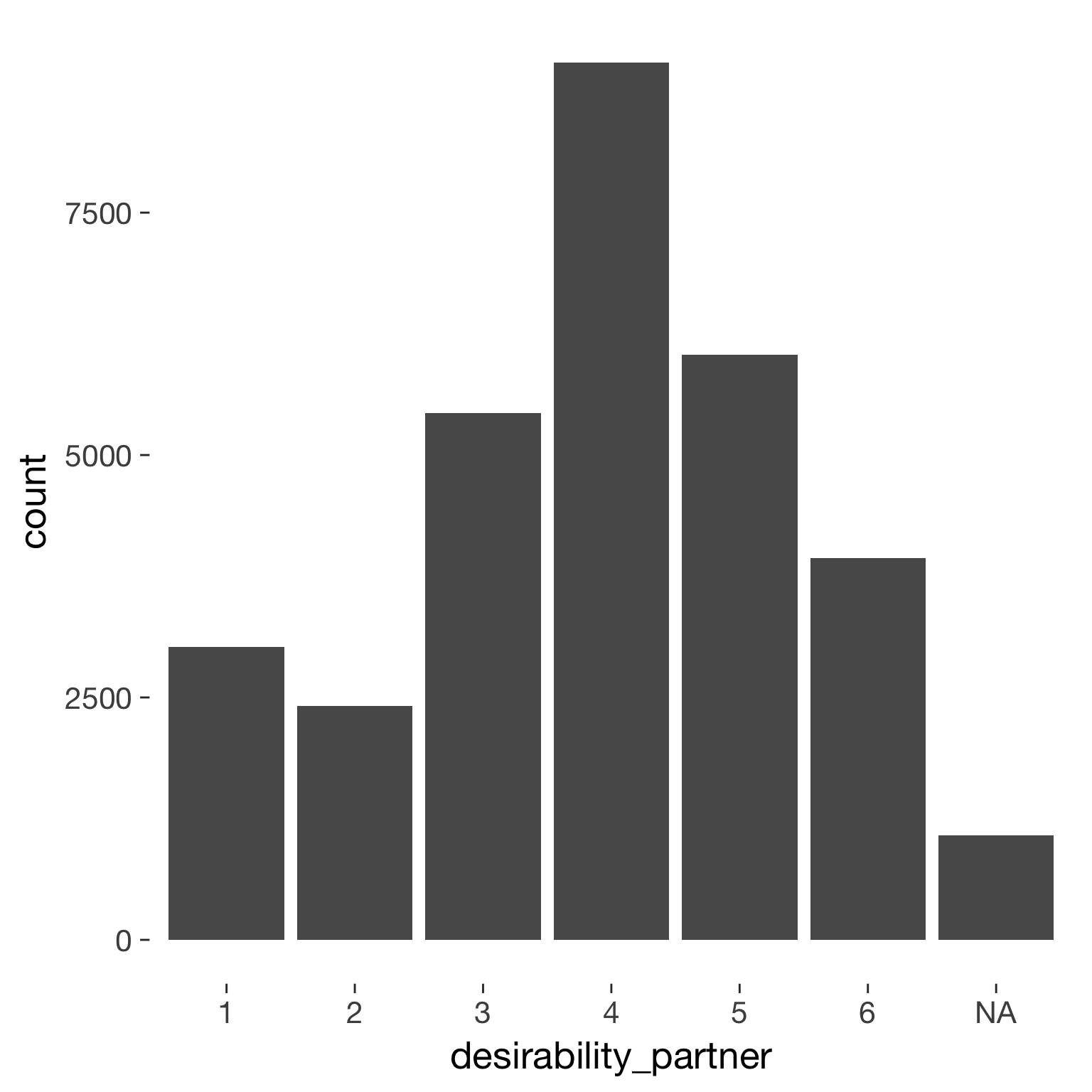
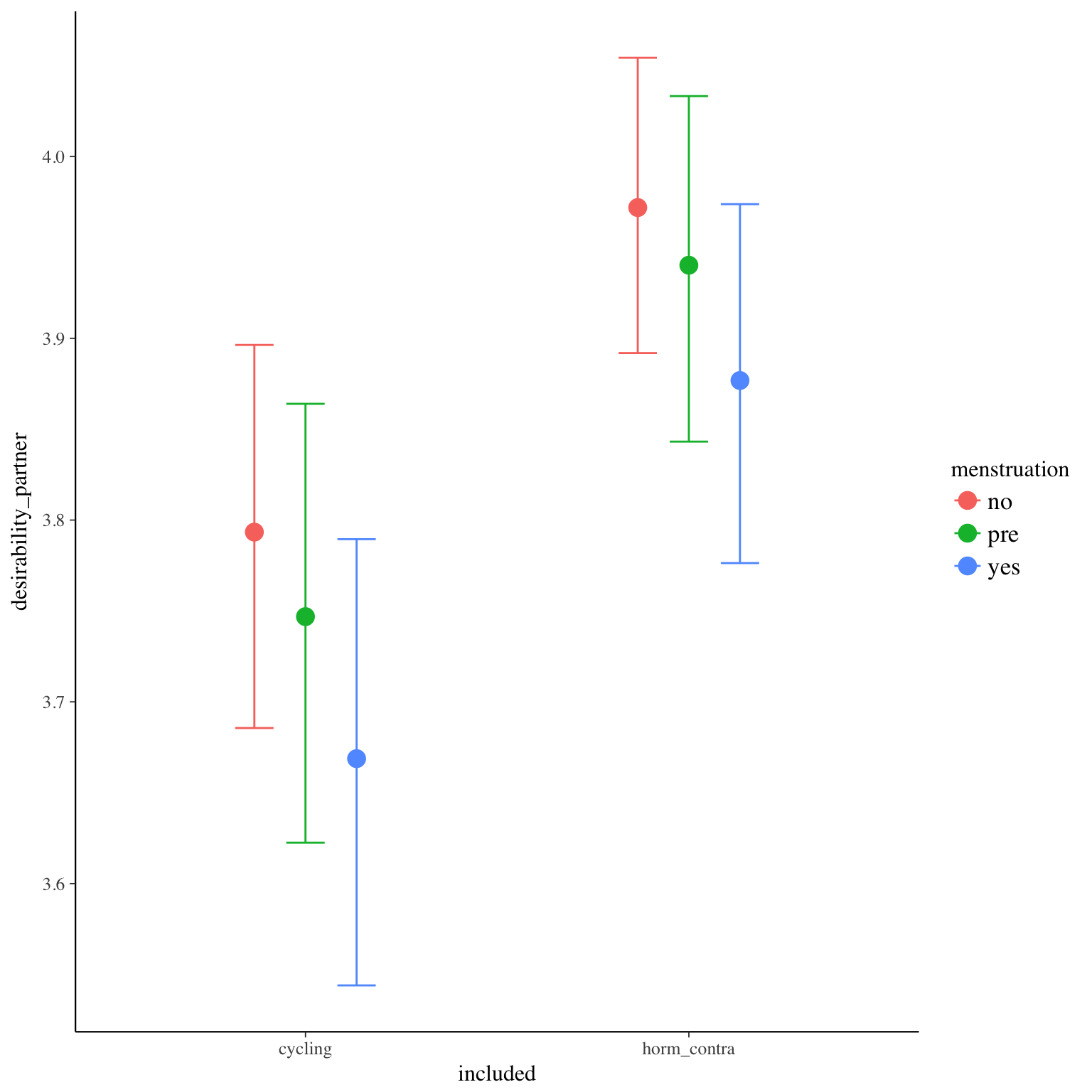
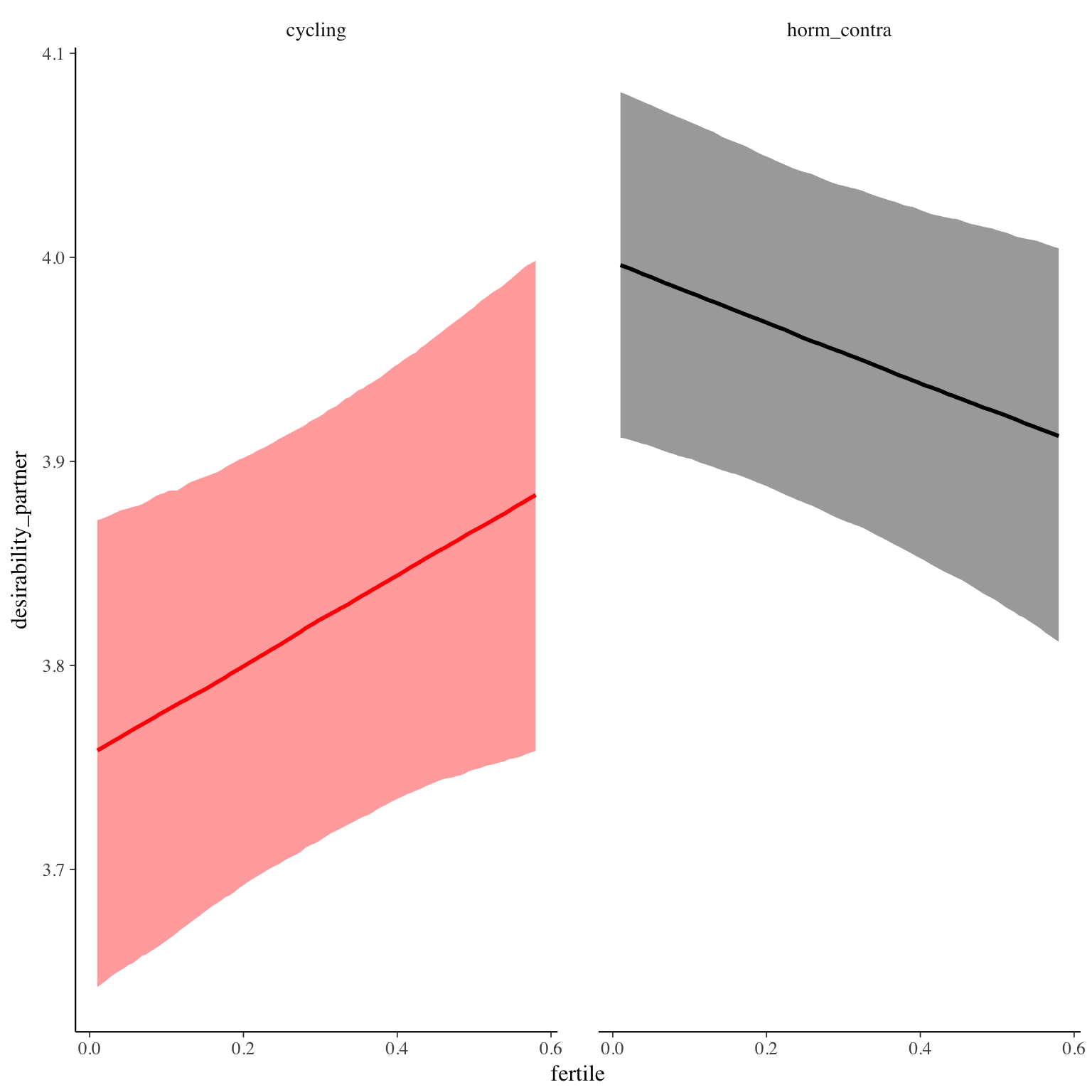
desirability_partner
Item text:
…fand ich meinen Partner besonders sexuell anziehend.
Item translation:
26. I found my partner sexually desirable.
Choices:
| choice | value | frequency | percent |
|---|---|---|---|
| 1 | Stimme nicht zu | 3019 | 0.1 |
| 2 | Stimme überwiegend nicht zu | 2413 | 0.08 |
| 3 | Stimme eher nicht zu | 5435 | 0.18 |
| 4 | Stimme eher zu | 9046 | 0.3 |
| 5 | Stimme überwiegend zu | 6032 | 0.2 |
| 6 | Stimme voll zu | 3934 | 0.13 |
Model
Model summary
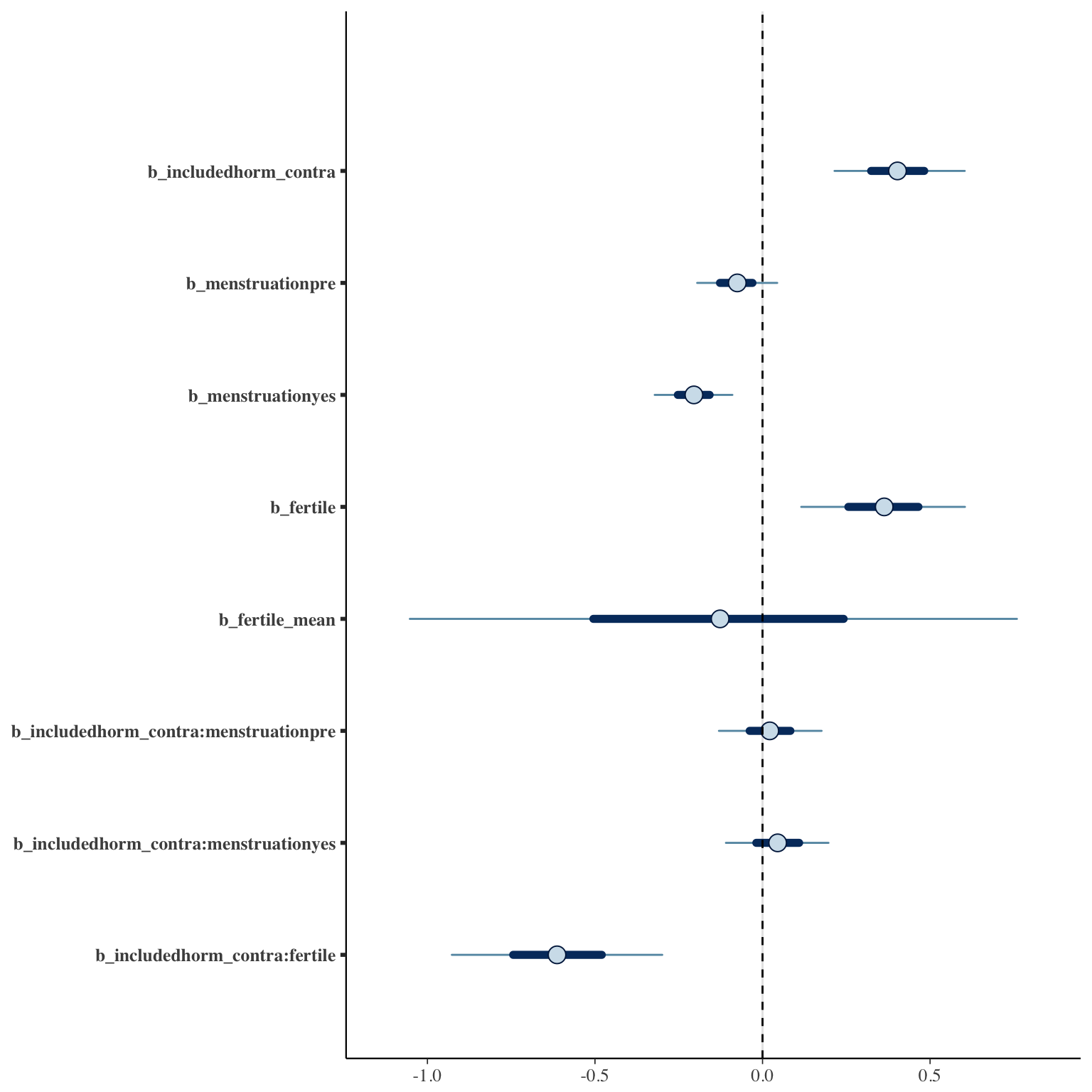
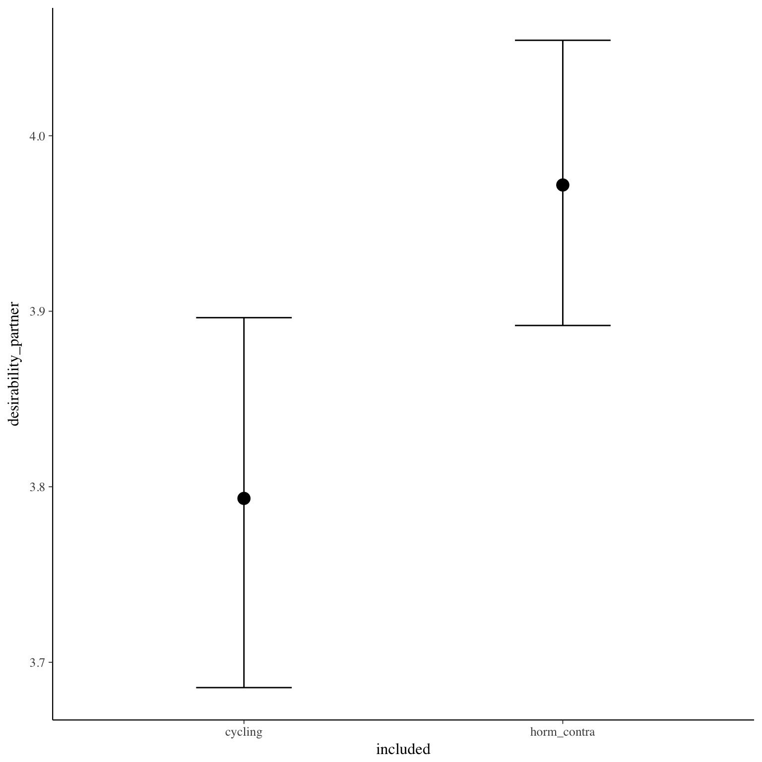
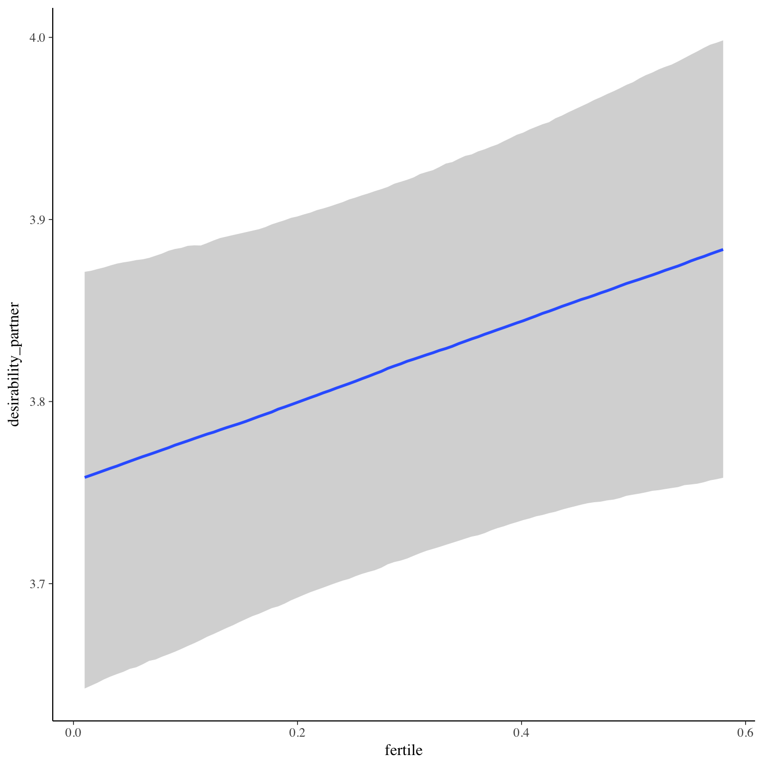
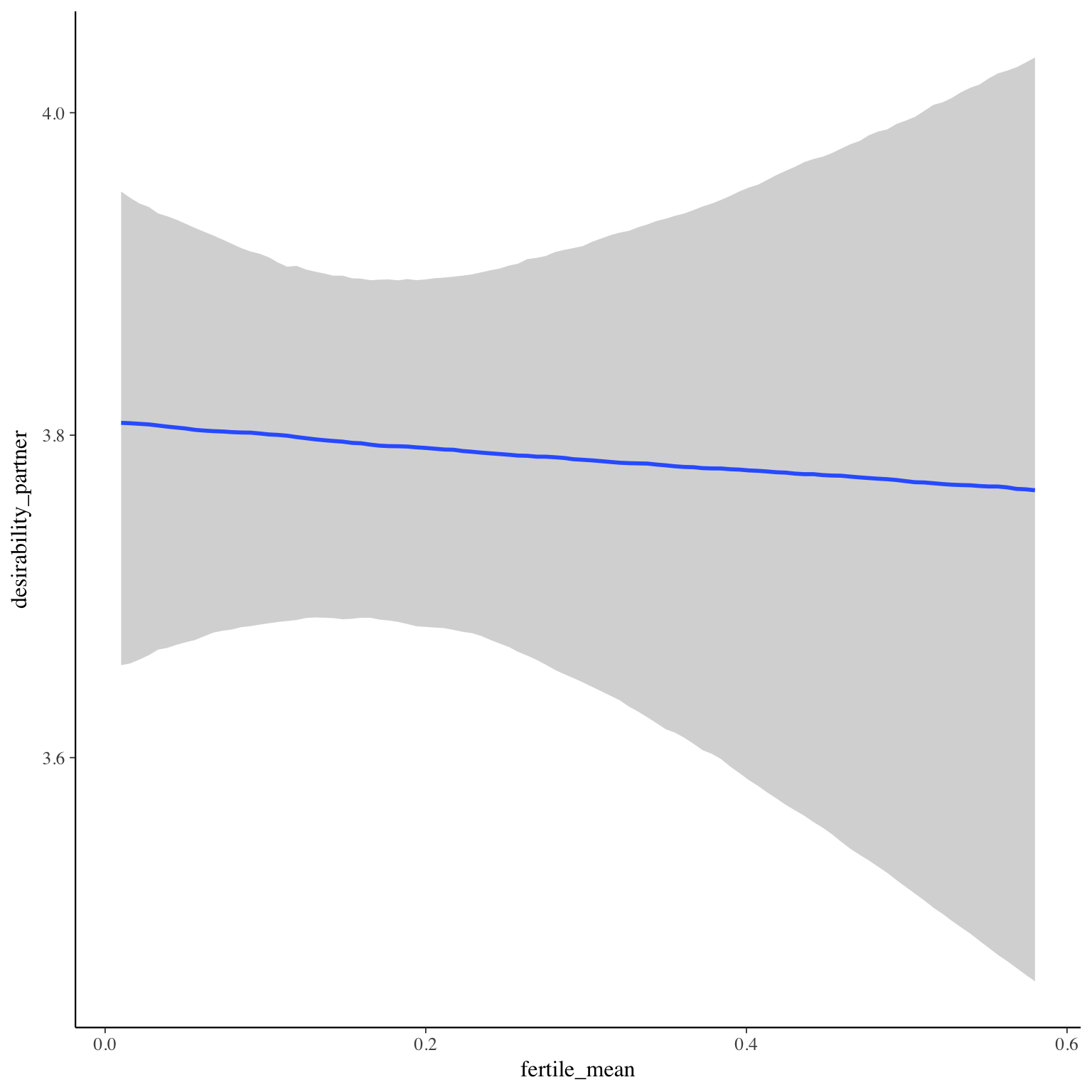
 Family: cumulative(logit)
Formula: desirability_partner ~ included * (menstruation + fertile) + fertile_mean + (1 + fertile + menstruation | person)
         disc = 1
   Data: diary (Number of observations: 26548)
Samples: 4 chains, each with iter = 2000; warmup = 1000; thin = 1;
         total post-warmup samples = 4000
    ICs: LOO = 76199.22; WAIC = Not computed

Group-Level Effects:
~person (Number of levels: 1043)
                                     Estimate Est.Error l-95% CI u-95% CI Eff.Sample Rhat
sd(Intercept)                            1.73      0.05     1.64     1.83        714 1.01
sd(fertile)                              1.70      0.12     1.47     1.93        696 1.01
sd(menstruationpre)                      0.76      0.06     0.65     0.87        700 1.00
sd(menstruationyes)                      0.84      0.06     0.72     0.94        690 1.00
cor(Intercept,fertile)                  -0.26      0.06    -0.36    -0.14       1569 1.00
cor(Intercept,menstruationpre)          -0.17      0.07    -0.30    -0.03       1839 1.00
cor(fertile,menstruationpre)             0.24      0.09     0.05     0.39        494 1.01
cor(Intercept,menstruationyes)          -0.16      0.06    -0.28    -0.04       1618 1.00
cor(fertile,menstruationyes)             0.24      0.09     0.07     0.41        513 1.01
cor(menstruationpre,menstruationyes)     0.30      0.09     0.12     0.46        548 1.00

Population-Level Effects:
                                    Estimate Est.Error l-95% CI u-95% CI Eff.Sample Rhat
Intercept[1]                           -2.95      0.13    -3.22    -2.69        551 1.00
Intercept[2]                           -2.00      0.13    -2.26    -1.74        549 1.00
Intercept[3]                           -0.63      0.13    -0.89    -0.37        543 1.00
Intercept[4]                            1.20      0.13     0.94     1.46        548 1.00
Intercept[5]                            2.86      0.13     2.59     3.12        556 1.00
includedhorm_contra                     0.40      0.12     0.18     0.64        359 1.01
menstruationpre                        -0.08      0.07    -0.22     0.07       1528 1.00
menstruationyes                        -0.21      0.07    -0.34    -0.07       1643 1.00
fertile                                 0.36      0.15     0.07     0.65       1333 1.00
fertile_mean                           -0.14      0.56    -1.27     0.93        931 1.00
includedhorm_contra:menstruationpre     0.02      0.09    -0.16     0.21       1610 1.00
includedhorm_contra:menstruationyes     0.05      0.09    -0.13     0.23       1790 1.00
includedhorm_contra:fertile            -0.61      0.19    -1.00    -0.24       1364 1.00

Samples were drawn using sampling(NUTS). For each parameter, Eff.Sample
is a crude measure of effective sample size, and Rhat is the potential
scale reduction factor on split chains (at convergence, Rhat = 1).
Coefficient plot
Marginal effect plots

Diagnostics
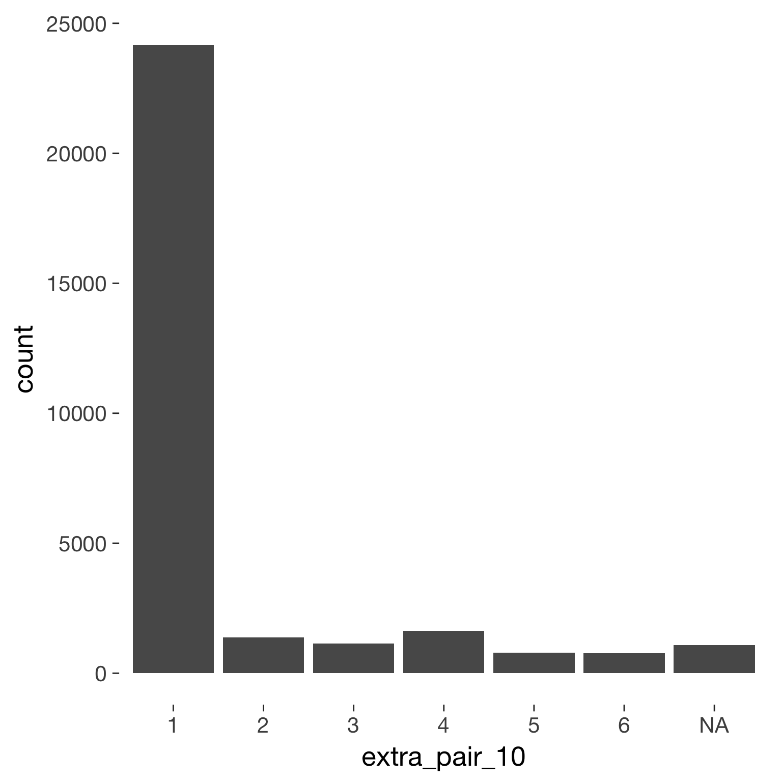
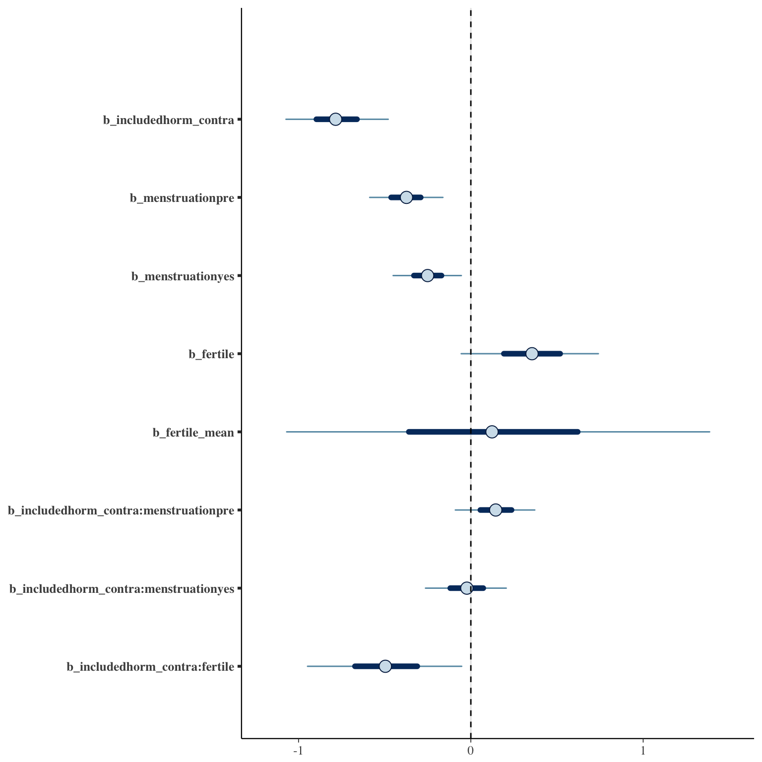
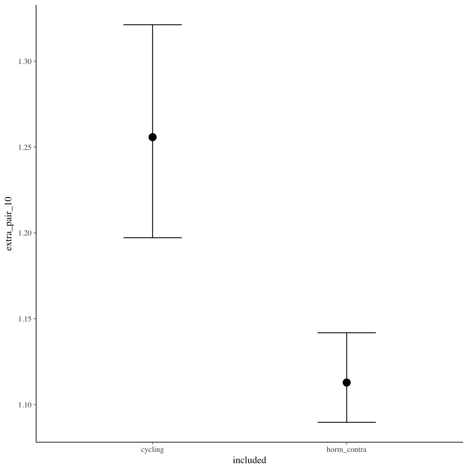
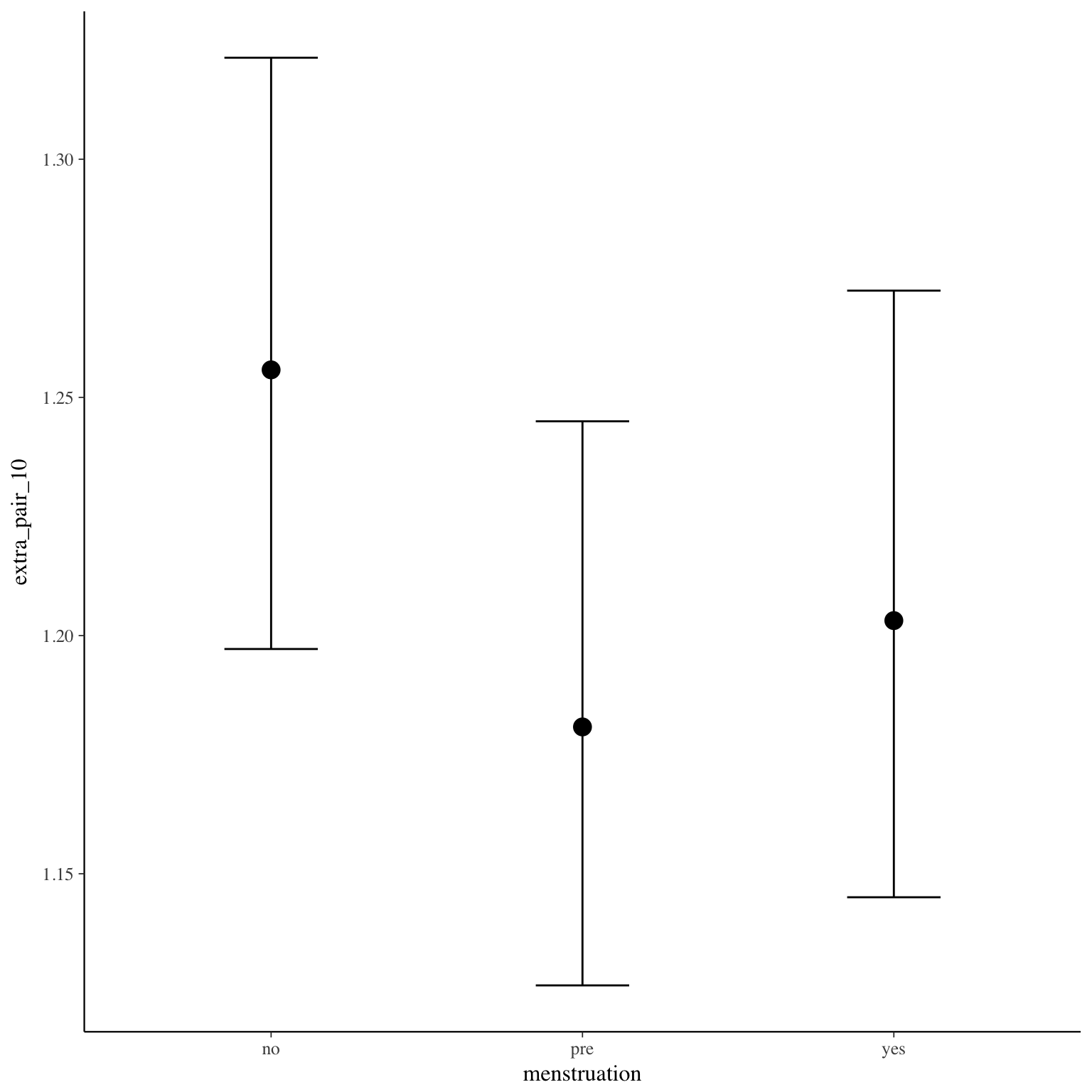
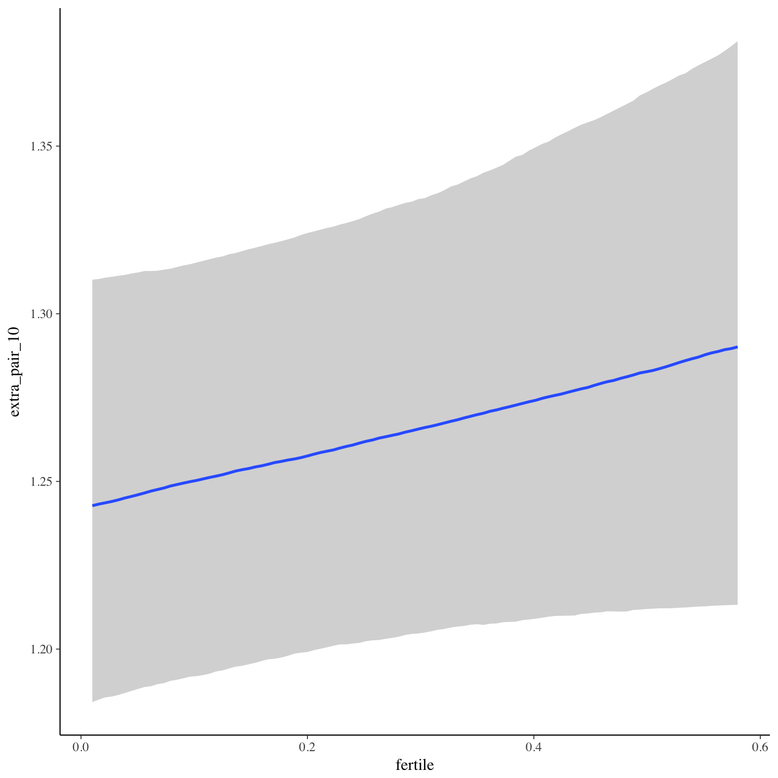
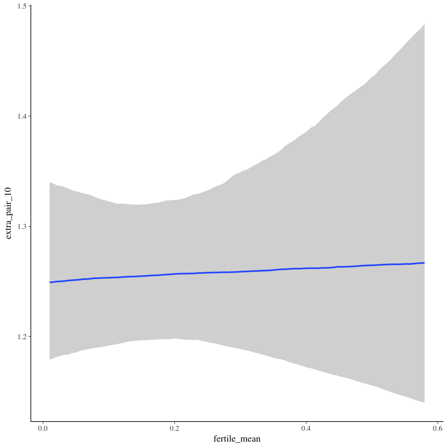
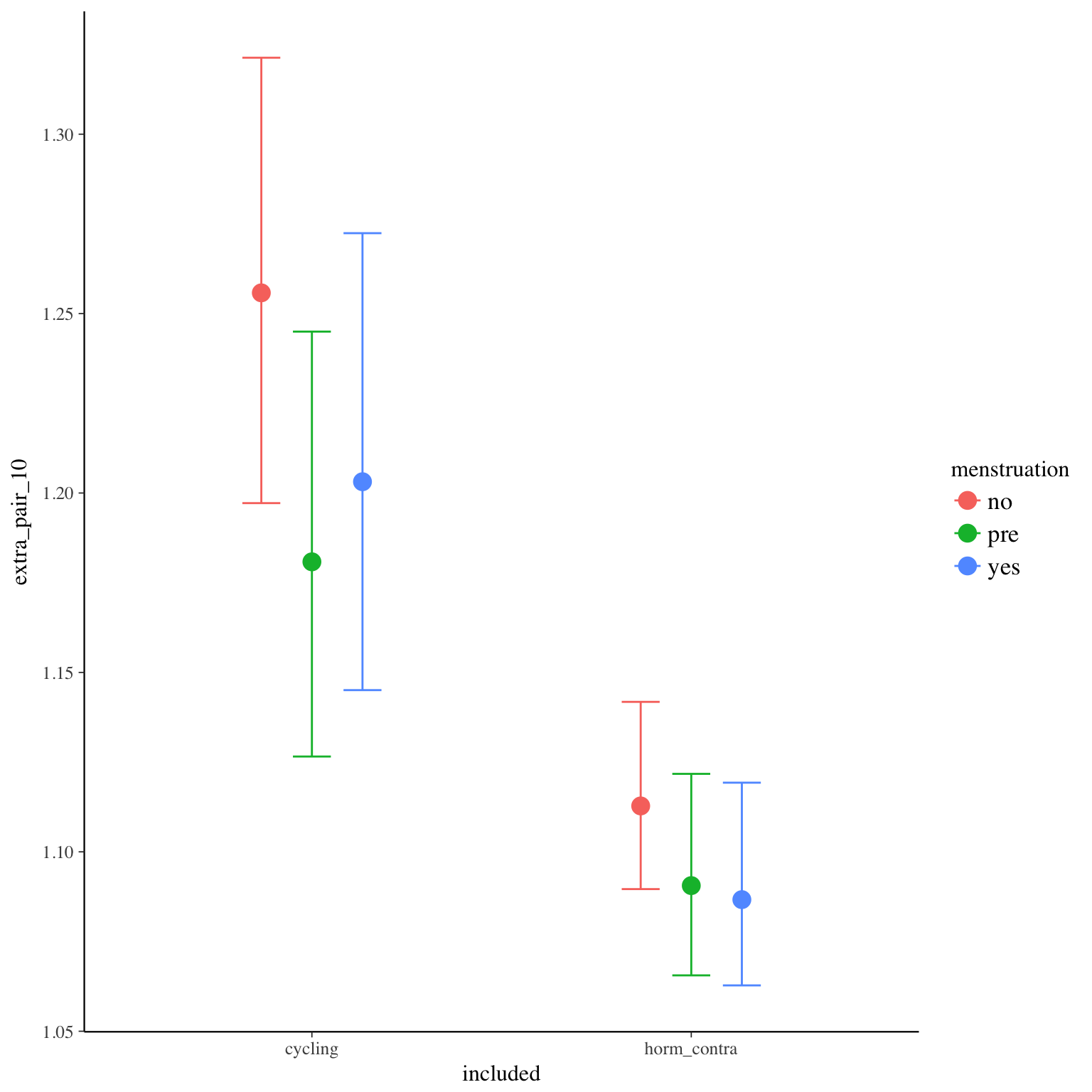
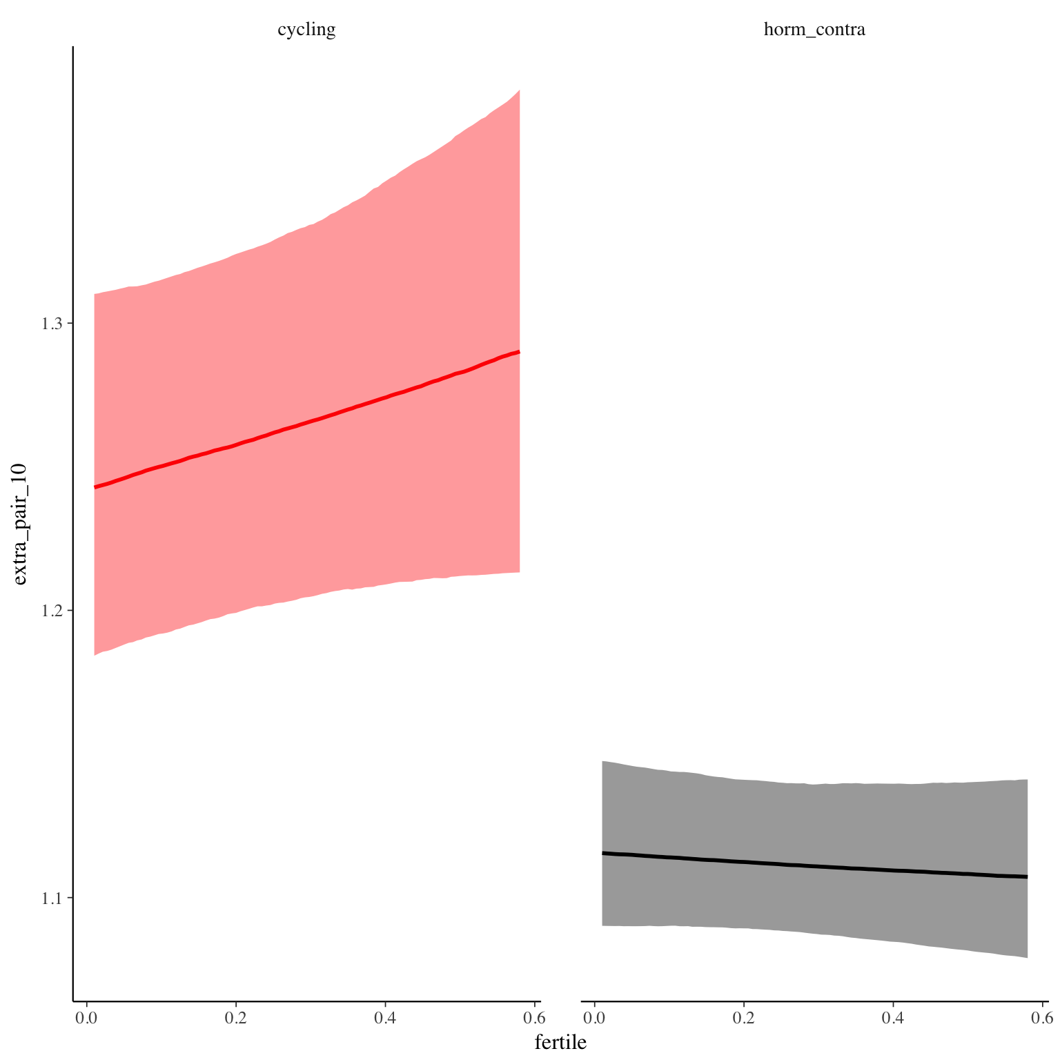
extra_pair_10
Item text:
… habe ich mich zu einem Freund, Bekannten oder Kollegen hingezogen gefühlt
Item translation:
54. I was attracted to a friend, acquaintance, or colleague.
Choices:
| choice | value | frequency | percent |
|---|---|---|---|
| 1 | Stimme nicht zu | 24168 | 0.81 |
| 2 | Stimme überwiegend nicht zu | 1382 | 0.05 |
| 3 | Stimme eher nicht zu | 1145 | 0.04 |
| 4 | Stimme eher zu | 1629 | 0.05 |
| 5 | Stimme überwiegend zu | 781 | 0.03 |
| 6 | Stimme voll zu | 768 | 0.03 |
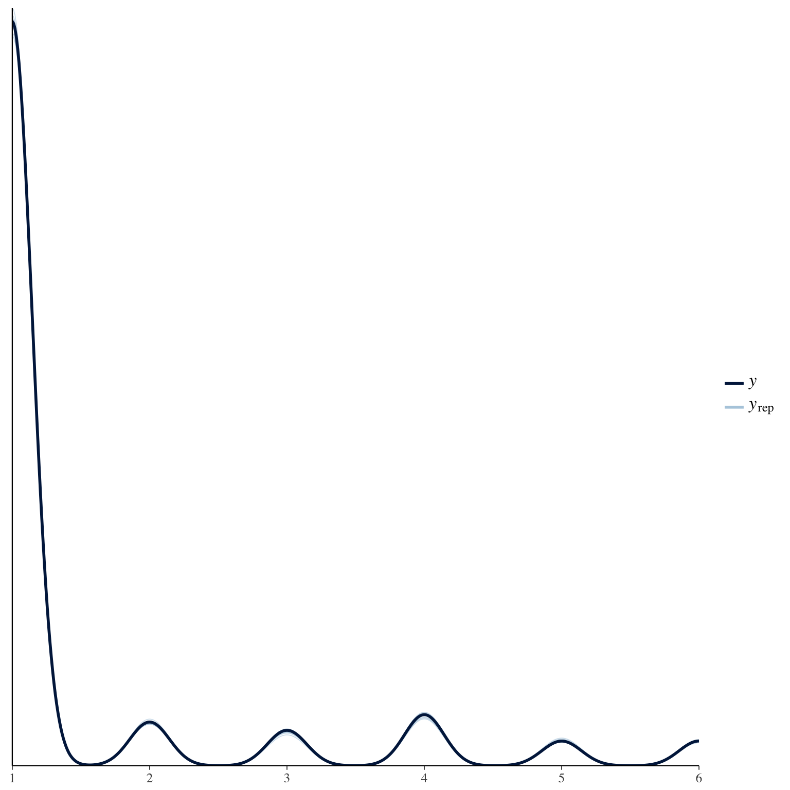
Model
Model summary
 Family: cumulative(logit)
Formula: extra_pair_10 ~ included * (menstruation + fertile) + fertile_mean + (1 + fertile + menstruation | person)
         disc = 1
   Data: diary (Number of observations: 26544)
Samples: 4 chains, each with iter = 2000; warmup = 1000; thin = 1;
         total post-warmup samples = 4000
    ICs: LOO = 31332.22; WAIC = Not computed

Group-Level Effects:
~person (Number of levels: 1043)
                                     Estimate Est.Error l-95% CI u-95% CI Eff.Sample Rhat
sd(Intercept)                            2.46      0.10     2.28     2.65        753 1.01
sd(fertile)                              1.85      0.21     1.45     2.25        324 1.02
sd(menstruationpre)                      0.74      0.11     0.52     0.96        497 1.01
sd(menstruationyes)                      0.95      0.10     0.74     1.16        860 1.01
cor(Intercept,fertile)                  -0.10      0.11    -0.30     0.12       1607 1.00
cor(Intercept,menstruationpre)           0.07      0.14    -0.21     0.34       1590 1.00
cor(fertile,menstruationpre)             0.06      0.17    -0.29     0.36        233 1.02
cor(Intercept,menstruationyes)           0.03      0.11    -0.19     0.24       1394 1.00
cor(fertile,menstruationyes)             0.40      0.11     0.17     0.61        396 1.01
cor(menstruationpre,menstruationyes)     0.65      0.12     0.39     0.86        439 1.01

Population-Level Effects:
                                    Estimate Est.Error l-95% CI u-95% CI Eff.Sample Rhat
Intercept[1]                            2.05      0.19     1.68     2.44        668 1.00
Intercept[2]                            2.63      0.19     2.26     3.01        675 1.00
Intercept[3]                            3.20      0.19     2.83     3.59        680 1.00
Intercept[4]                            4.44      0.19     4.06     4.83        685 1.00
Intercept[5]                            5.55      0.20     5.15     5.95        710 1.00
includedhorm_contra                    -0.78      0.18    -1.15    -0.42        354 1.01
menstruationpre                        -0.38      0.13    -0.64    -0.12       1805 1.00
menstruationyes                        -0.25      0.12    -0.50    -0.01       1965 1.00
fertile                                 0.35      0.24    -0.13     0.82       1901 1.00
fertile_mean                            0.14      0.75    -1.35     1.64       1166 1.00
includedhorm_contra:menstruationpre     0.14      0.14    -0.14     0.41       1680 1.00
includedhorm_contra:menstruationyes    -0.02      0.14    -0.31     0.25       1640 1.00
includedhorm_contra:fertile            -0.50      0.27    -1.04     0.02       1721 1.00

Samples were drawn using sampling(NUTS). For each parameter, Eff.Sample
is a crude measure of effective sample size, and Rhat is the potential
scale reduction factor on split chains (at convergence, Rhat = 1).
Coefficient plot
Marginal effect plots
Diagnostics
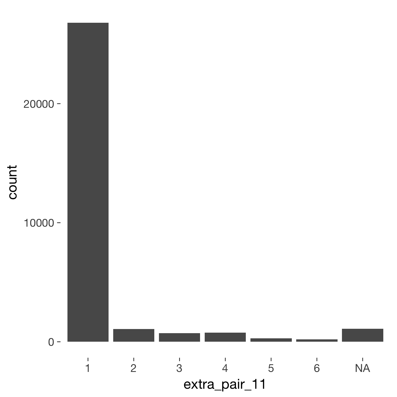
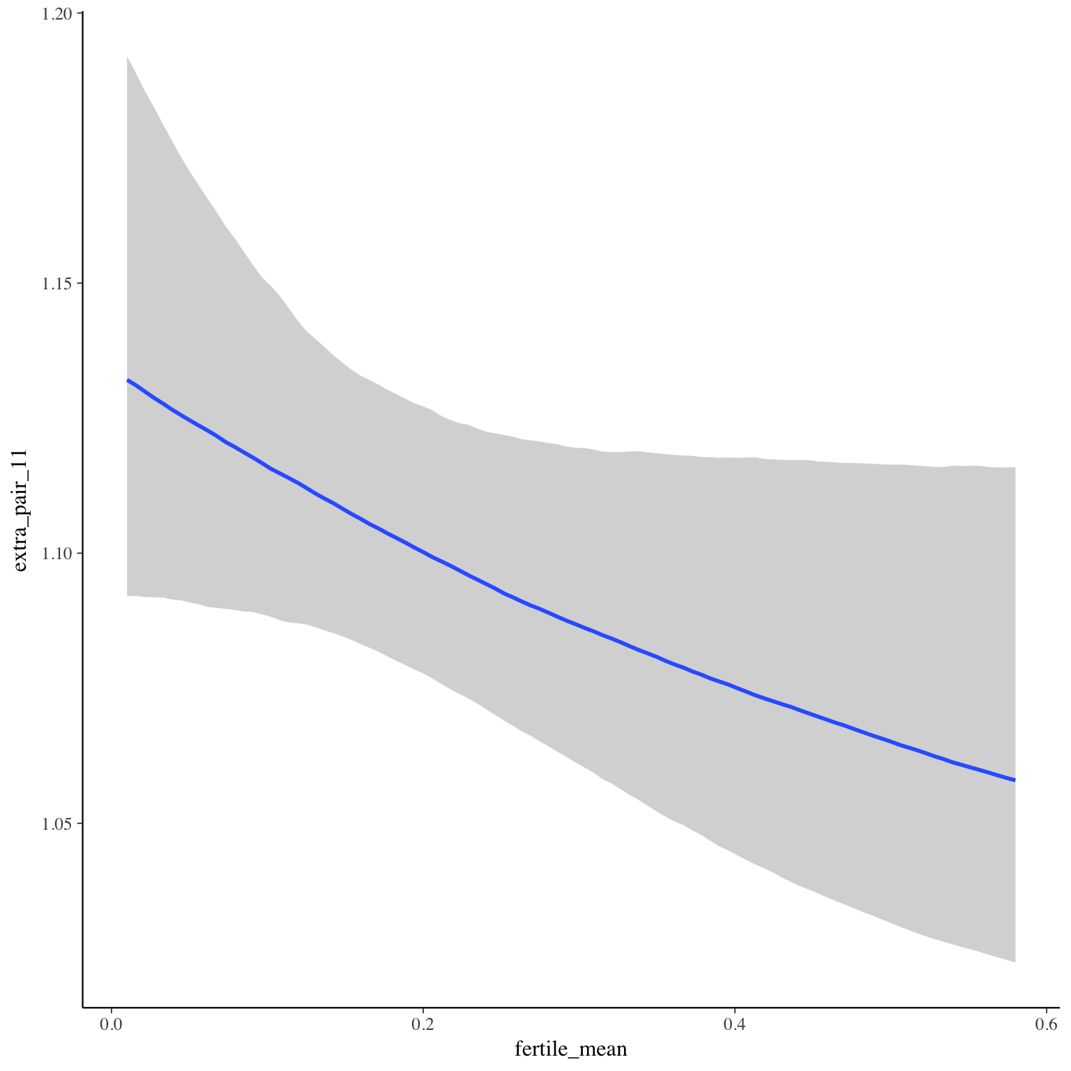
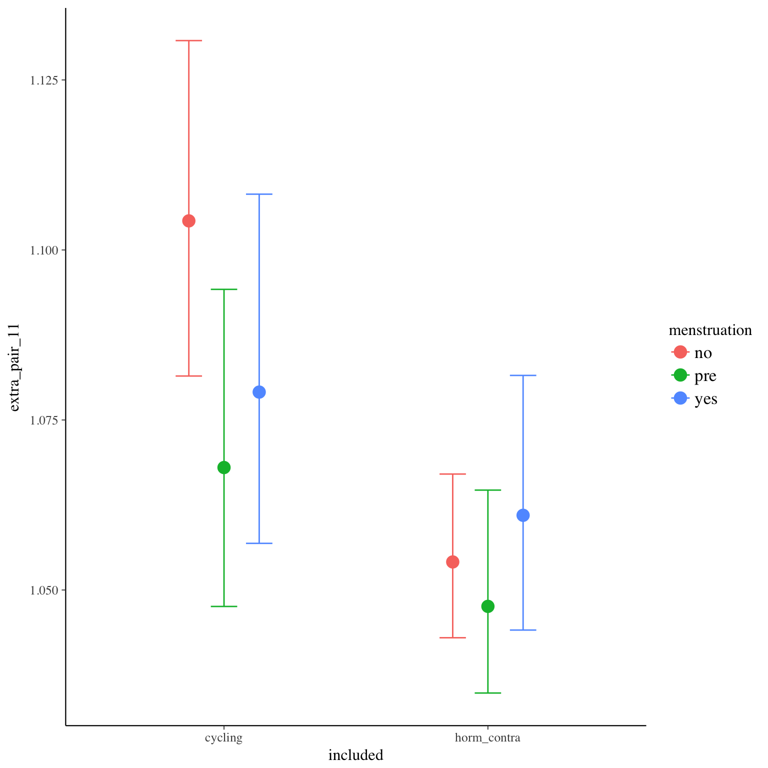
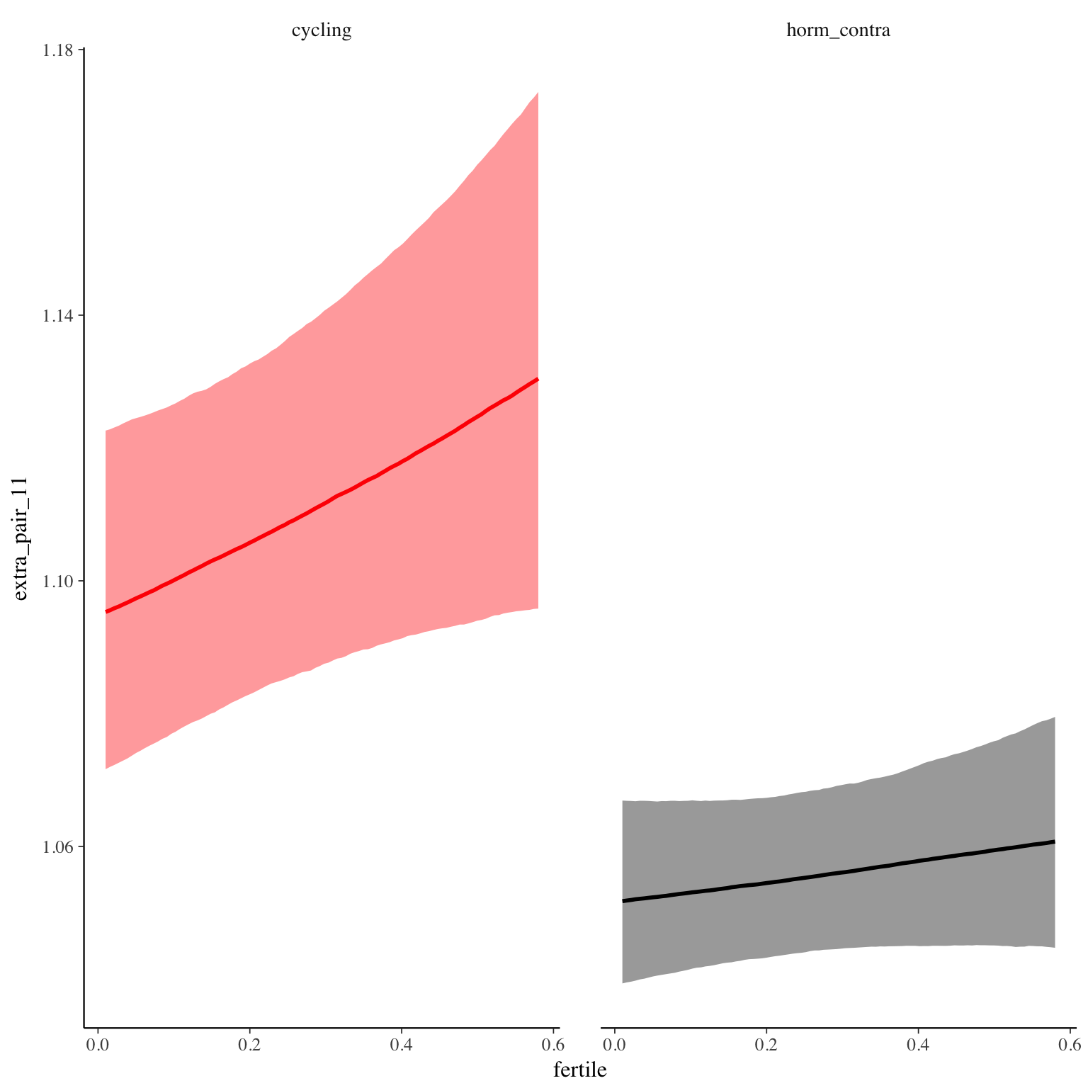
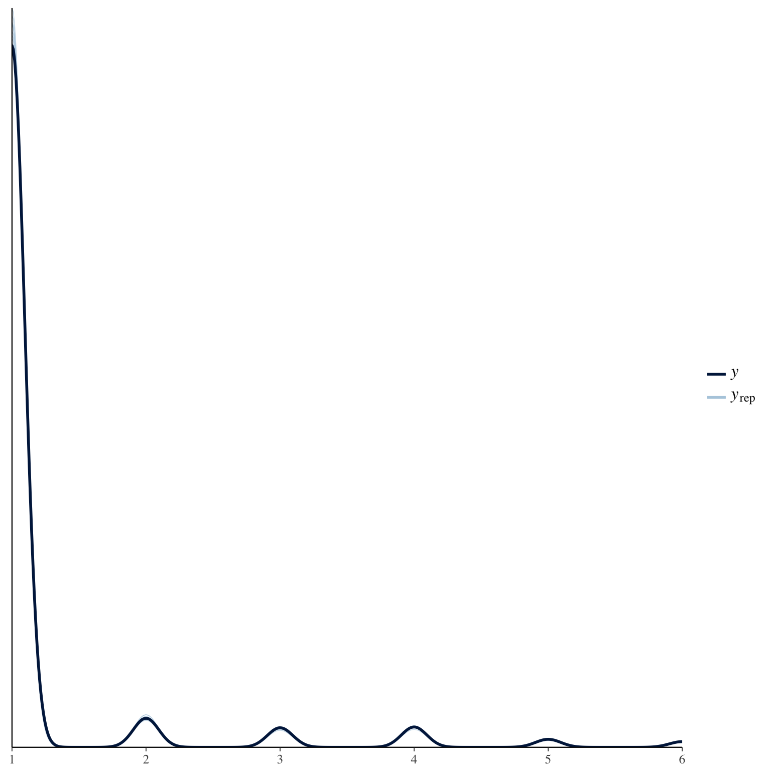
extra_pair_11
Item text:
… habe ich mich zu einem Mann hingezogen gefühlt, den ich nicht kannte.
Item translation:
55. I was attracted to a stranger.
Choices:
| choice | value | frequency | percent |
|---|---|---|---|
| 1 | Stimme nicht zu | 26789 | 0.9 |
| 2 | Stimme überwiegend nicht zu | 1080 | 0.04 |
| 3 | Stimme eher nicht zu | 728 | 0.02 |
| 4 | Stimme eher zu | 773 | 0.03 |
| 5 | Stimme überwiegend zu | 299 | 0.01 |
| 6 | Stimme voll zu | 204 | 0.01 |
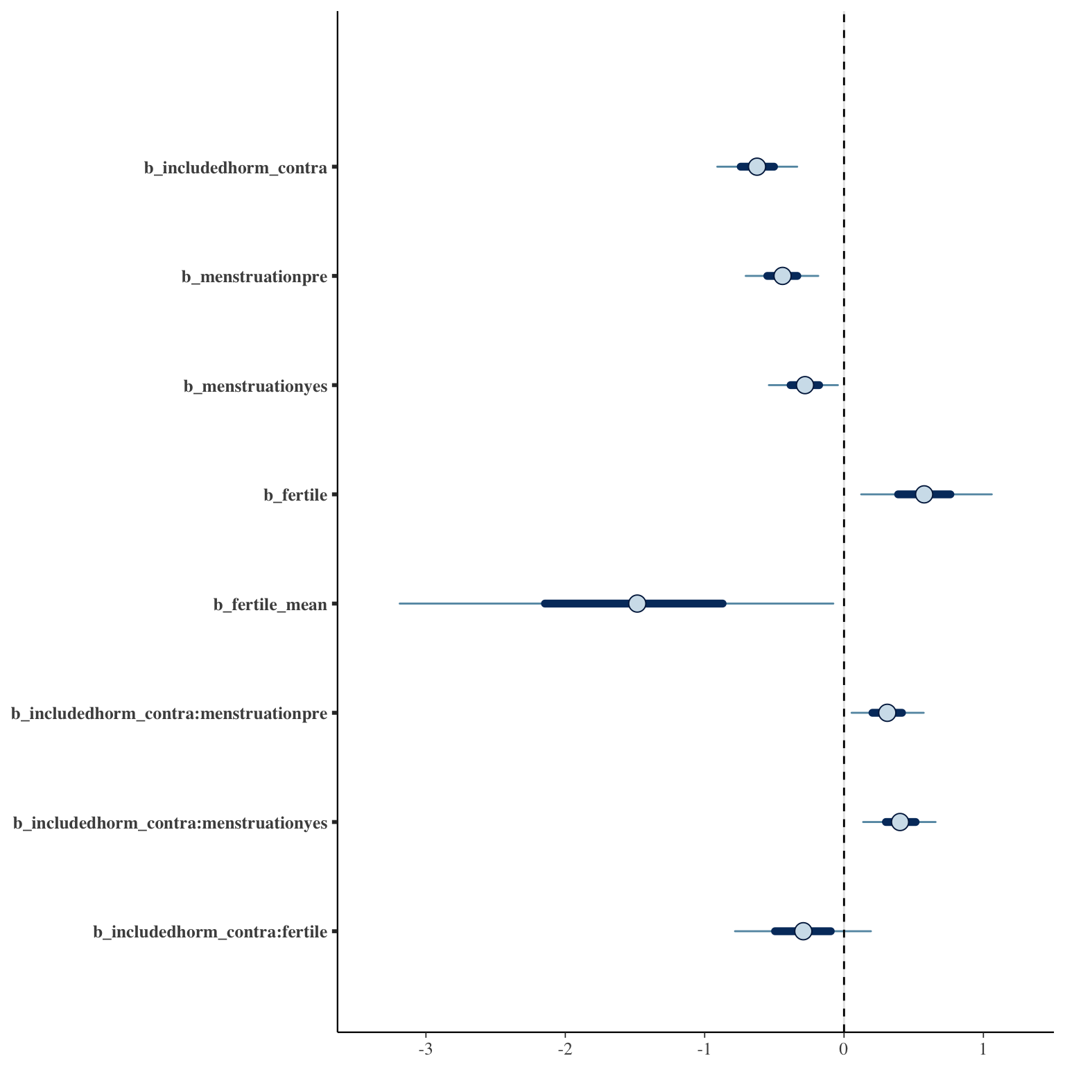
Model
Model summary
 Family: cumulative(logit)
Formula: extra_pair_11 ~ included * (menstruation + fertile) + fertile_mean + (1 + fertile + menstruation | person)
         disc = 1
   Data: diary (Number of observations: 26544)
Samples: 4 chains, each with iter = 2000; warmup = 1000; thin = 1;
         total post-warmup samples = 4000
    ICs: LOO = 20657.91; WAIC = Not computed

Group-Level Effects:
~person (Number of levels: 1043)
                                     Estimate Est.Error l-95% CI u-95% CI Eff.Sample Rhat
sd(Intercept)                            2.16      0.10     1.97     2.36        782 1.00
sd(fertile)                              1.55      0.29     0.96     2.09        355 1.01
sd(menstruationpre)                      0.61      0.15     0.31     0.89        448 1.00
sd(menstruationyes)                      0.78      0.13     0.53     1.03        564 1.01
cor(Intercept,fertile)                  -0.41      0.13    -0.64    -0.14       1847 1.00
cor(Intercept,menstruationpre)          -0.32      0.17    -0.63     0.05       2298 1.00
cor(fertile,menstruationpre)             0.41      0.24    -0.14     0.80        407 1.01
cor(Intercept,menstruationyes)          -0.30      0.14    -0.56    -0.01       1722 1.00
cor(fertile,menstruationyes)             0.33      0.21    -0.13     0.69        335 1.01
cor(menstruationpre,menstruationyes)     0.84      0.12     0.56     0.98        389 1.01

Population-Level Effects:
                                    Estimate Est.Error l-95% CI u-95% CI Eff.Sample Rhat
Intercept[1]                            2.70      0.21     2.27     3.10       1132 1.01
Intercept[2]                            3.37      0.21     2.94     3.78       1133 1.01
Intercept[3]                            3.99      0.21     3.56     4.40       1144 1.00
Intercept[4]                            5.14      0.22     4.71     5.56       1177 1.00
Intercept[5]                            6.20      0.23     5.75     6.63       1278 1.00
includedhorm_contra                    -0.62      0.17    -0.96    -0.28        900 1.00
menstruationpre                        -0.44      0.16    -0.76    -0.14       2402 1.00
menstruationyes                        -0.28      0.15    -0.60     0.00       2255 1.00
fertile                                 0.58      0.28     0.02     1.15       2033 1.00
fertile_mean                           -1.54      0.95    -3.59     0.14       1485 1.01
includedhorm_contra:menstruationpre     0.31      0.16     0.00     0.62       2753 1.00
includedhorm_contra:menstruationyes     0.40      0.16     0.09     0.71       2497 1.00
includedhorm_contra:fertile            -0.29      0.30    -0.87     0.28       2432 1.00

Samples were drawn using sampling(NUTS). For each parameter, Eff.Sample
is a crude measure of effective sample size, and Rhat is the potential
scale reduction factor on split chains (at convergence, Rhat = 1).
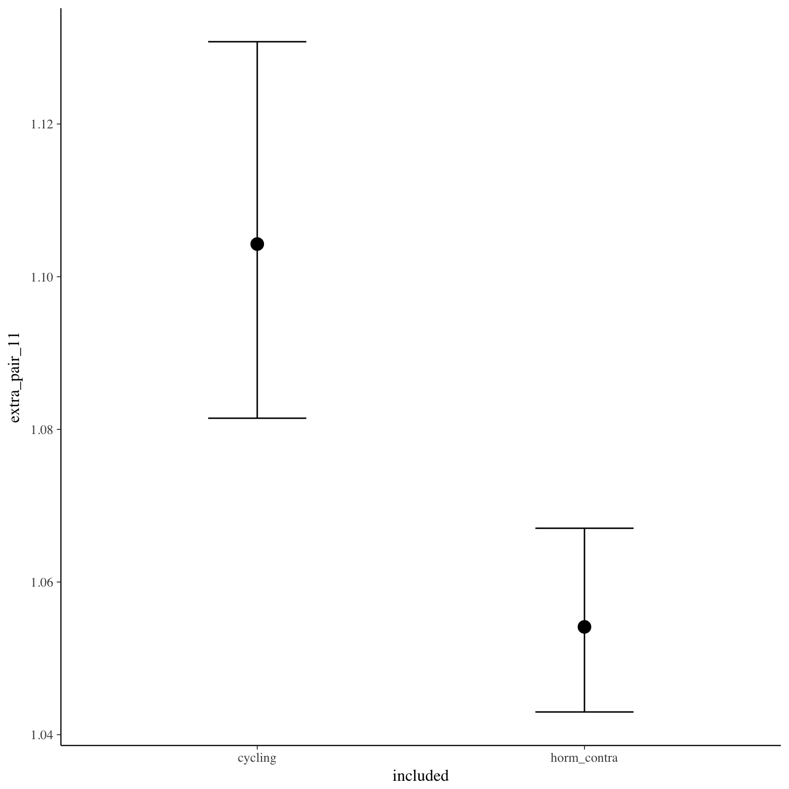
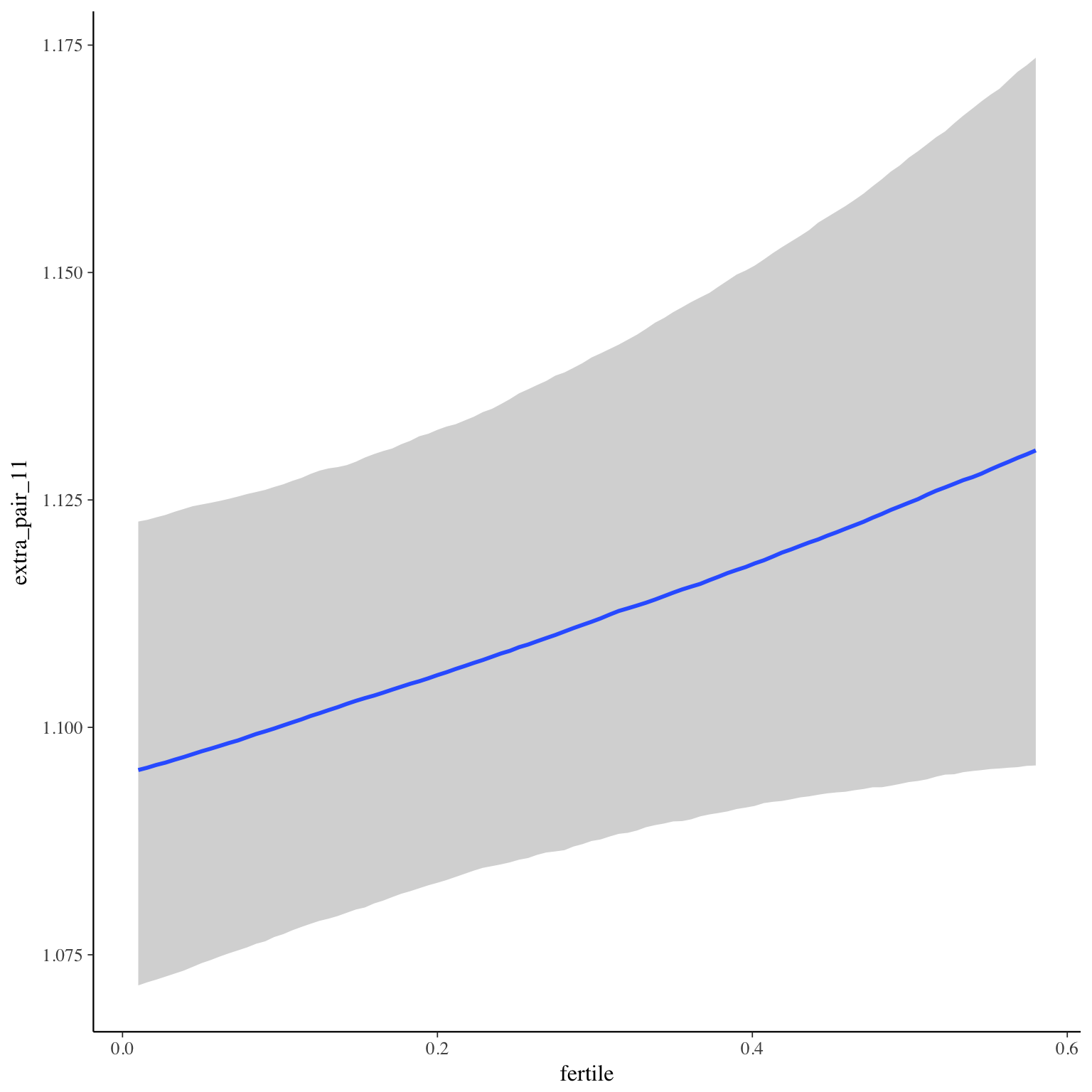
Coefficient plot
Marginal effect plots

Diagnostics
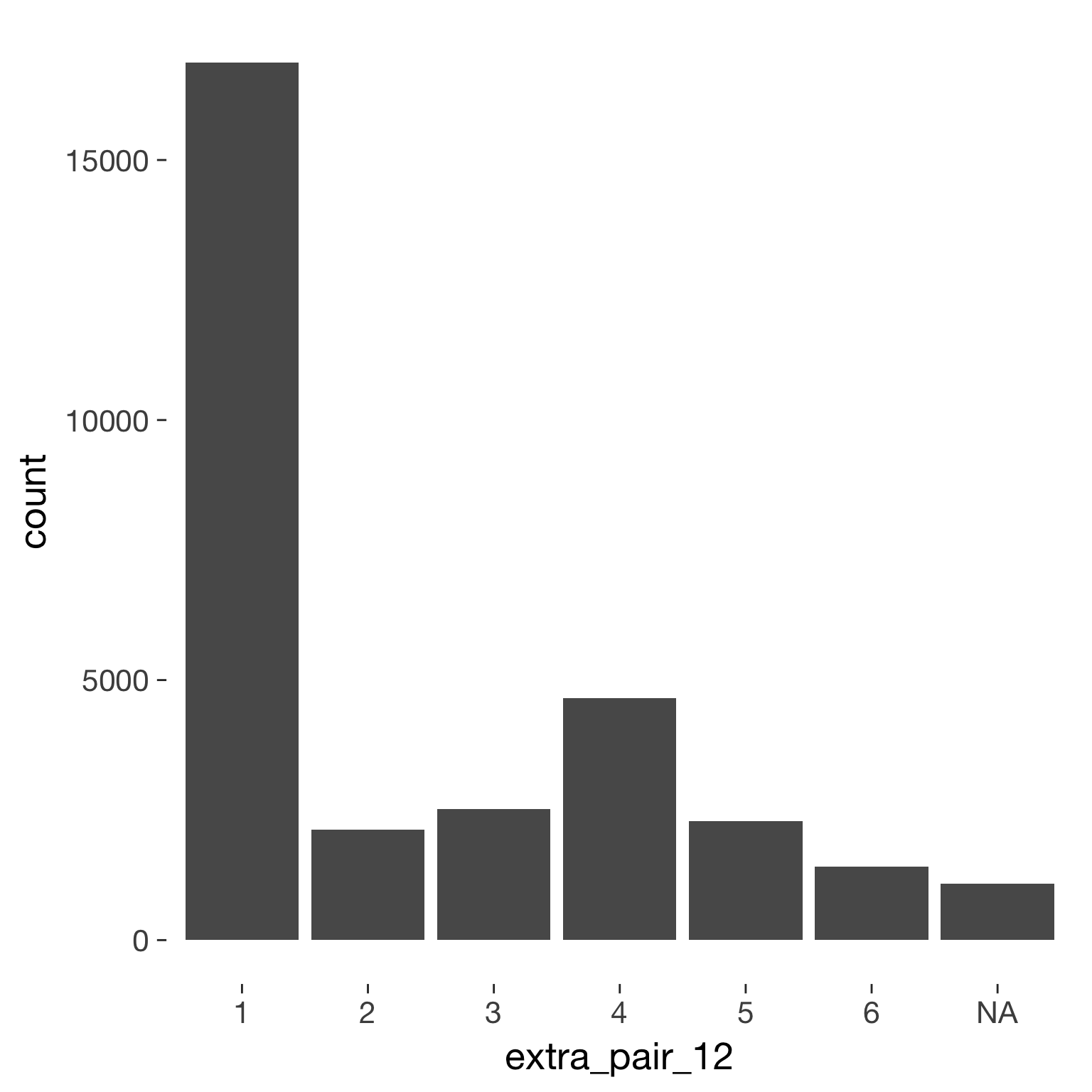
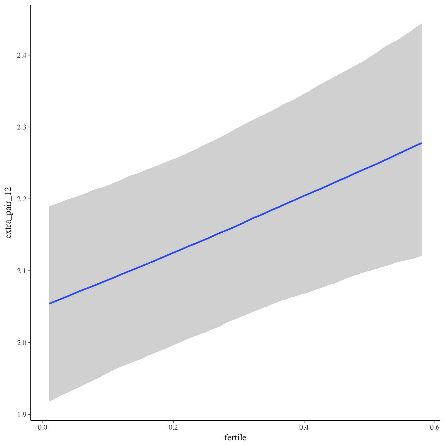
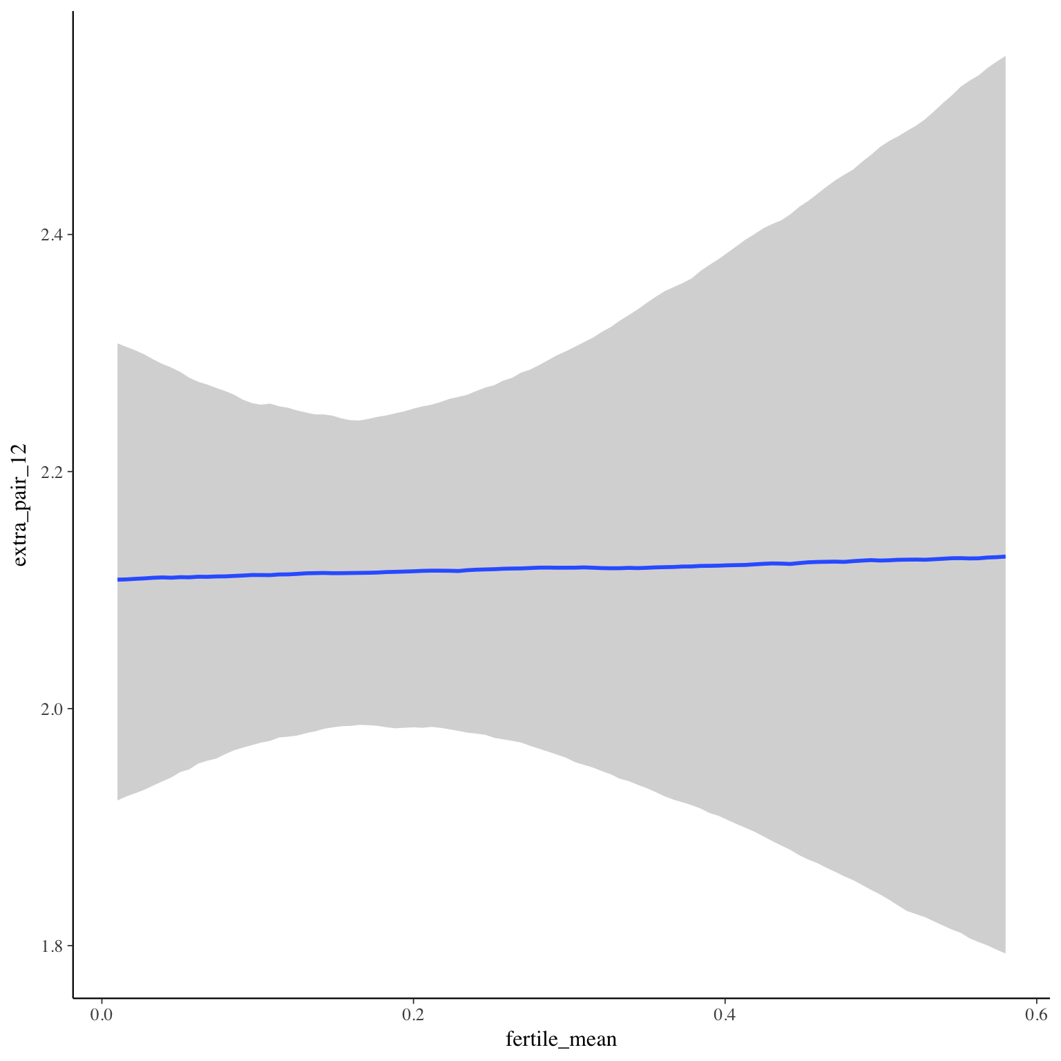
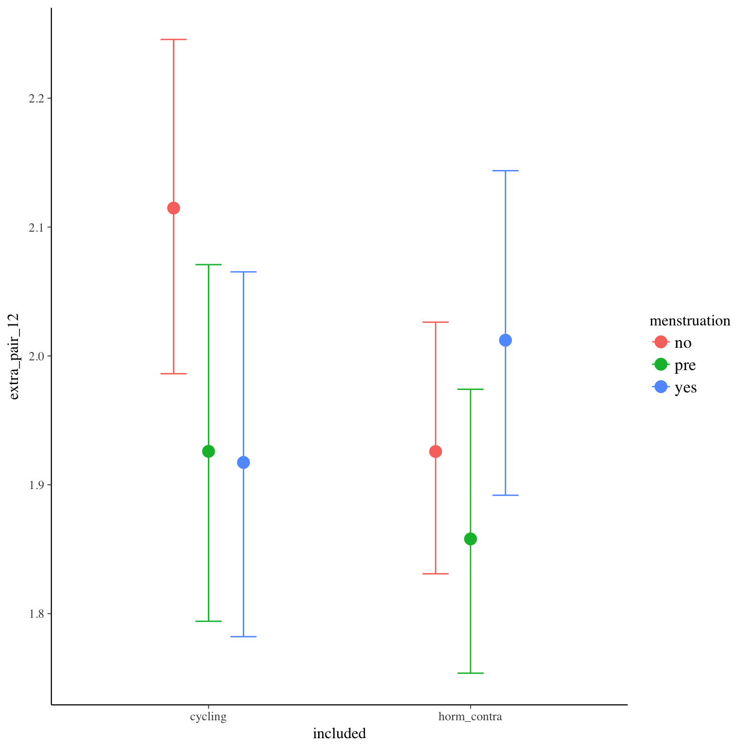
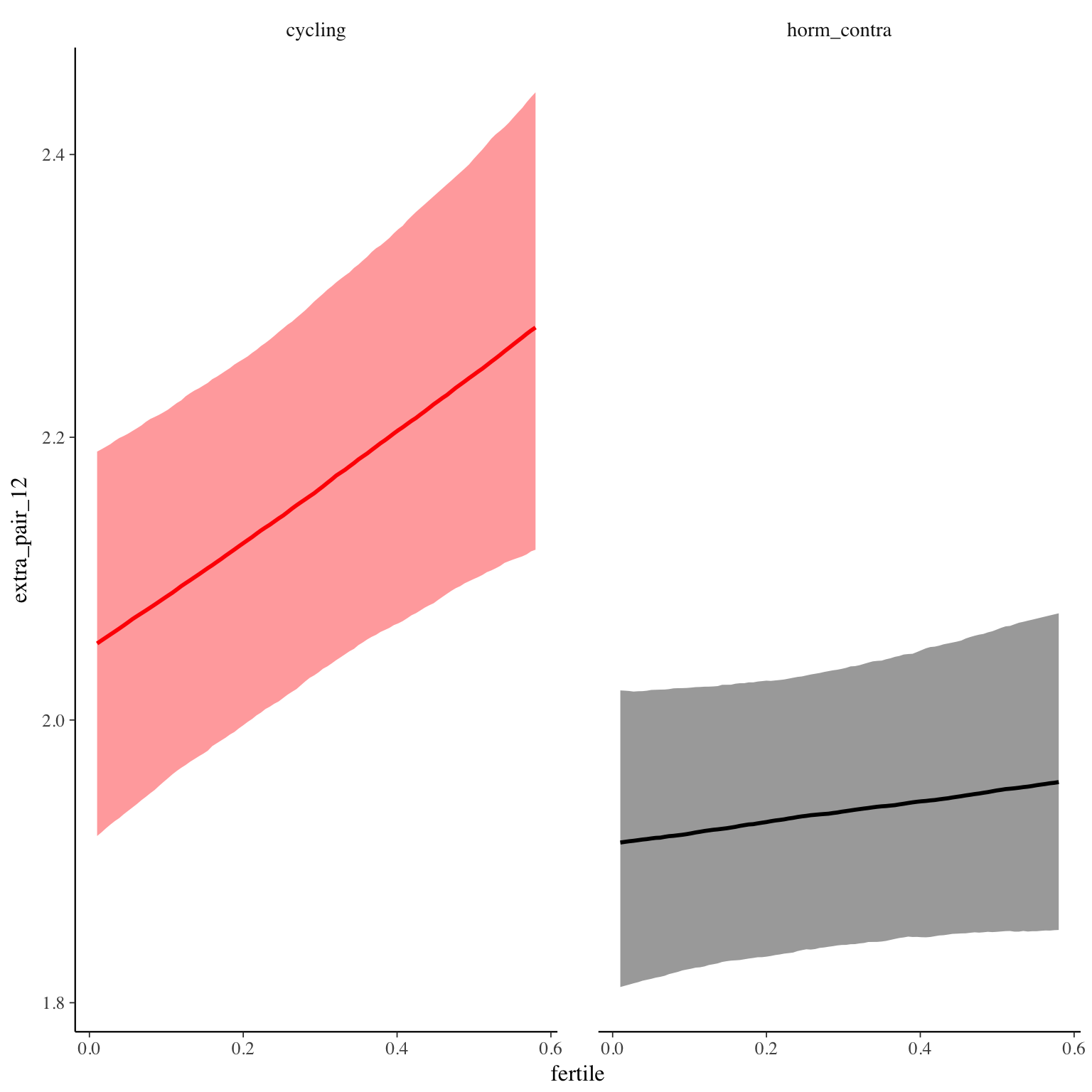
extra_pair_12
Item text:
… sind mir attraktive Männer in meiner Umgebung aufgefallen.
Item translation:
56. I noticed attractive men around me.
Choices:
| choice | value | frequency | percent |
|---|---|---|---|
| 1 | Stimme nicht zu | 16870 | 0.56 |
| 2 | Stimme überwiegend nicht zu | 2130 | 0.07 |
| 3 | Stimme eher nicht zu | 2522 | 0.08 |
| 4 | Stimme eher zu | 4655 | 0.16 |
| 5 | Stimme überwiegend zu | 2281 | 0.08 |
| 6 | Stimme voll zu | 1415 | 0.05 |
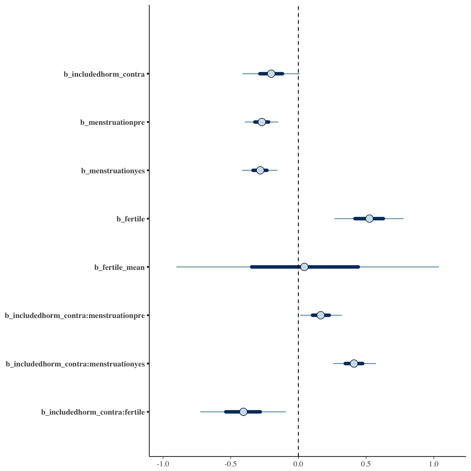
Model
Model summary
 Family: cumulative(logit)
Formula: extra_pair_12 ~ included * (menstruation + fertile) + fertile_mean + (1 + fertile + menstruation | person)
         disc = 1
   Data: diary (Number of observations: 26544)
Samples: 4 chains, each with iter = 2000; warmup = 1000; thin = 1;
         total post-warmup samples = 4000
    ICs: LOO = 61689.6; WAIC = Not computed

Group-Level Effects:
~person (Number of levels: 1043)
                                     Estimate Est.Error l-95% CI u-95% CI Eff.Sample Rhat
sd(Intercept)                            1.69      0.06     1.58     1.80        714 1.01
sd(fertile)                              1.40      0.15     1.08     1.69        325 1.01
sd(menstruationpre)                      0.48      0.09     0.28     0.64        296 1.02
sd(menstruationyes)                      0.65      0.07     0.50     0.79        559 1.01
cor(Intercept,fertile)                  -0.20      0.08    -0.35    -0.02       1521 1.00
cor(Intercept,menstruationpre)          -0.12      0.13    -0.36     0.15       1438 1.01
cor(fertile,menstruationpre)             0.45      0.16     0.08     0.71        307 1.01
cor(Intercept,menstruationyes)          -0.05      0.10    -0.24     0.15       1384 1.00
cor(fertile,menstruationyes)             0.49      0.12     0.23     0.70        405 1.01
cor(menstruationpre,menstruationyes)     0.76      0.13     0.47     0.96        175 1.01

Population-Level Effects:
                                    Estimate Est.Error l-95% CI u-95% CI Eff.Sample Rhat
Intercept[1]                            0.29      0.14     0.02     0.57        671 1.00
Intercept[2]                            0.75      0.14     0.47     1.03        675 1.00
Intercept[3]                            1.31      0.14     1.03     1.59        680 1.00
Intercept[4]                            2.68      0.14     2.40     2.96        691 1.00
Intercept[5]                            3.97      0.14     3.70     4.26        711 1.00
includedhorm_contra                    -0.20      0.13    -0.46     0.05        486 1.01
menstruationpre                        -0.27      0.07    -0.42    -0.13       1681 1.00
menstruationyes                        -0.28      0.08    -0.44    -0.13       1564 1.00
fertile                                 0.52      0.16     0.22     0.83       1610 1.00
fertile_mean                            0.05      0.59    -1.08     1.22       1034 1.00
includedhorm_contra:menstruationpre     0.17      0.09    -0.01     0.35       1849 1.00
includedhorm_contra:menstruationyes     0.41      0.09     0.23     0.60       1756 1.00
includedhorm_contra:fertile            -0.41      0.19    -0.79    -0.04       1663 1.00

Samples were drawn using sampling(NUTS). For each parameter, Eff.Sample
is a crude measure of effective sample size, and Rhat is the potential
scale reduction factor on split chains (at convergence, Rhat = 1).
Coefficient plot
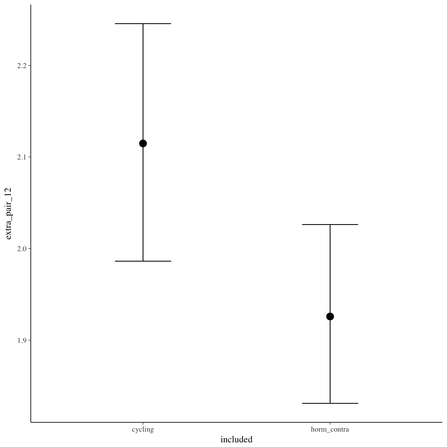
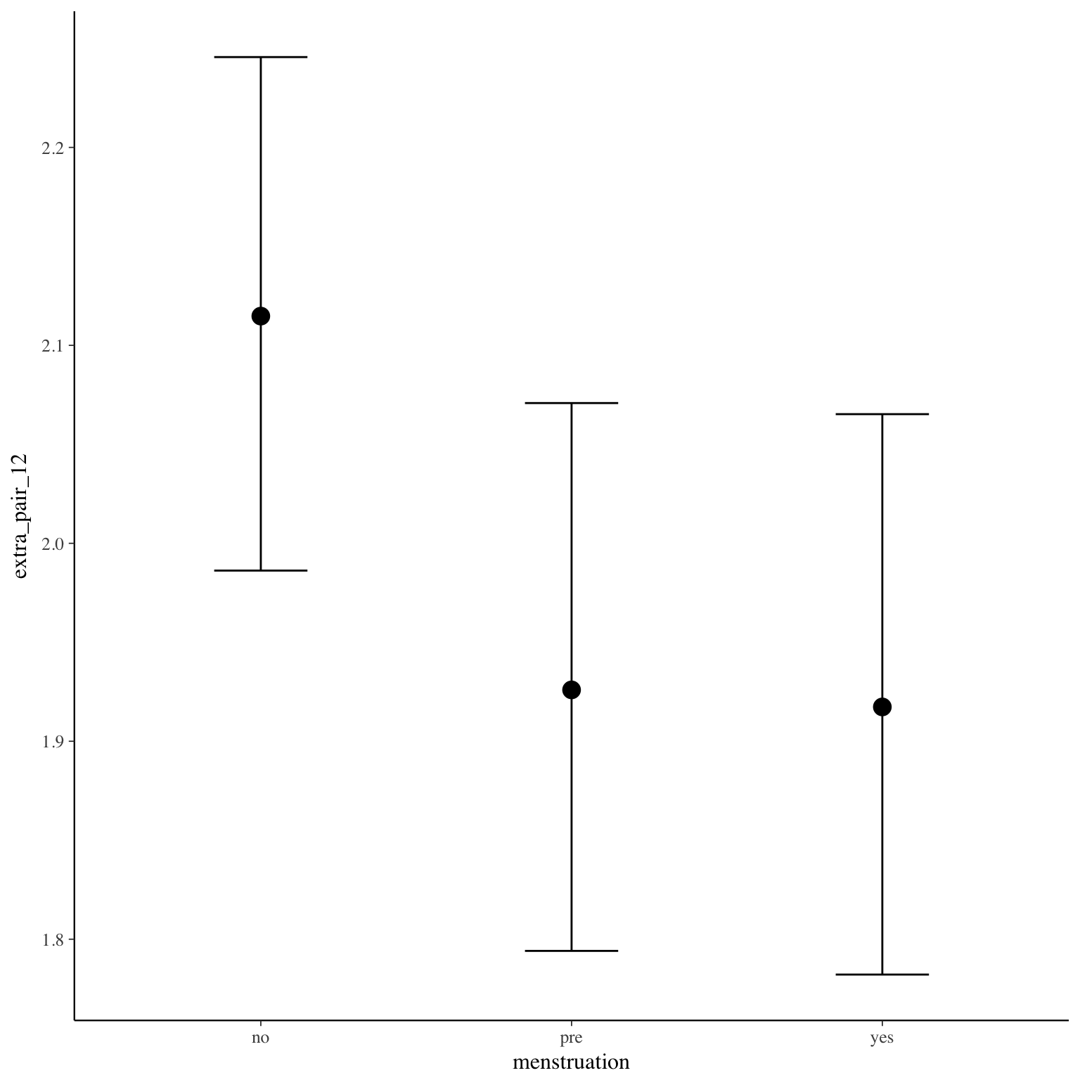
Marginal effect plots
Diagnostics
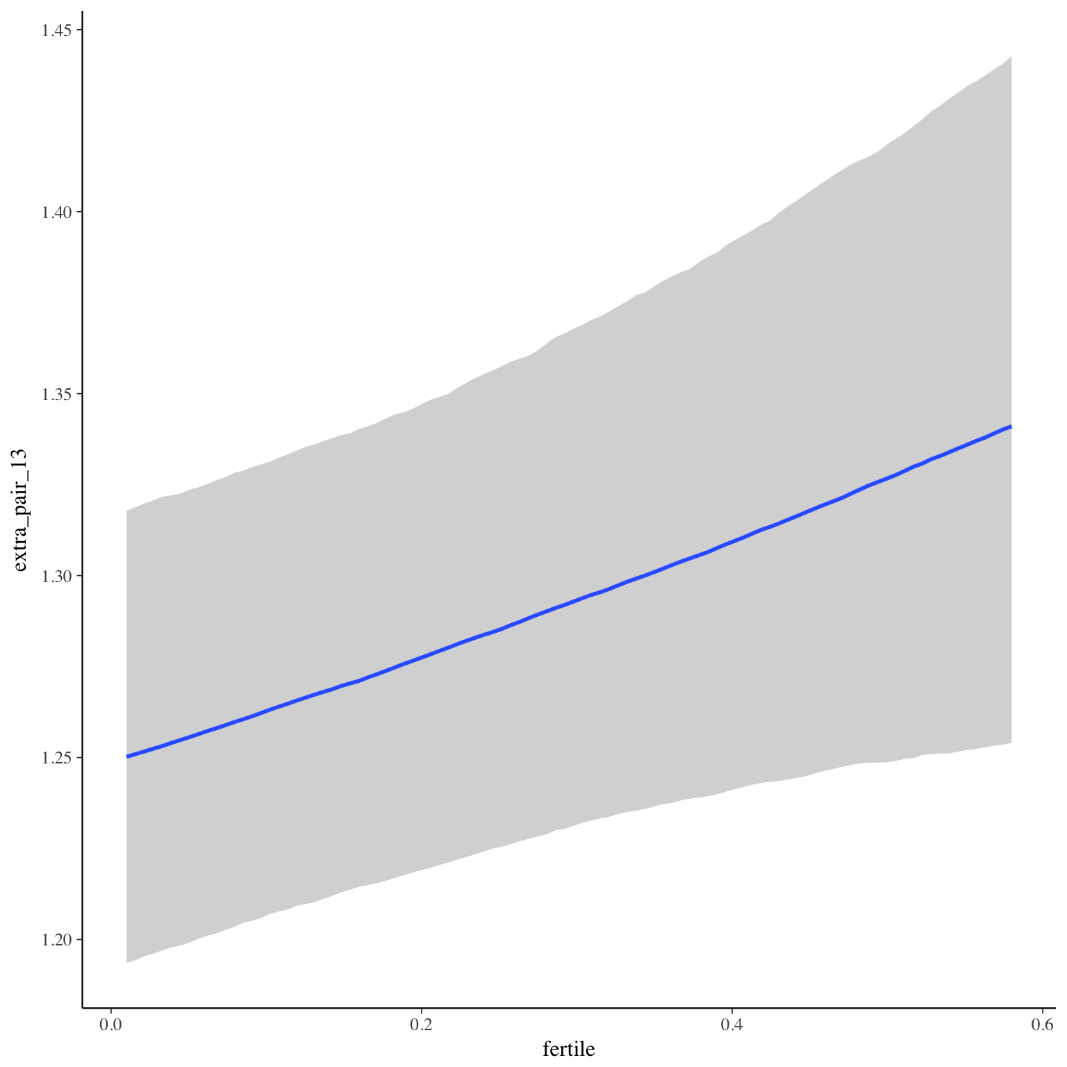
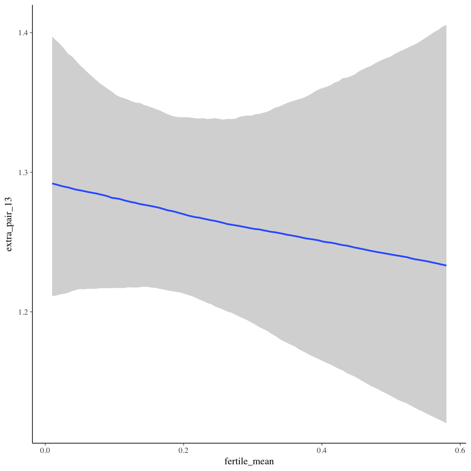
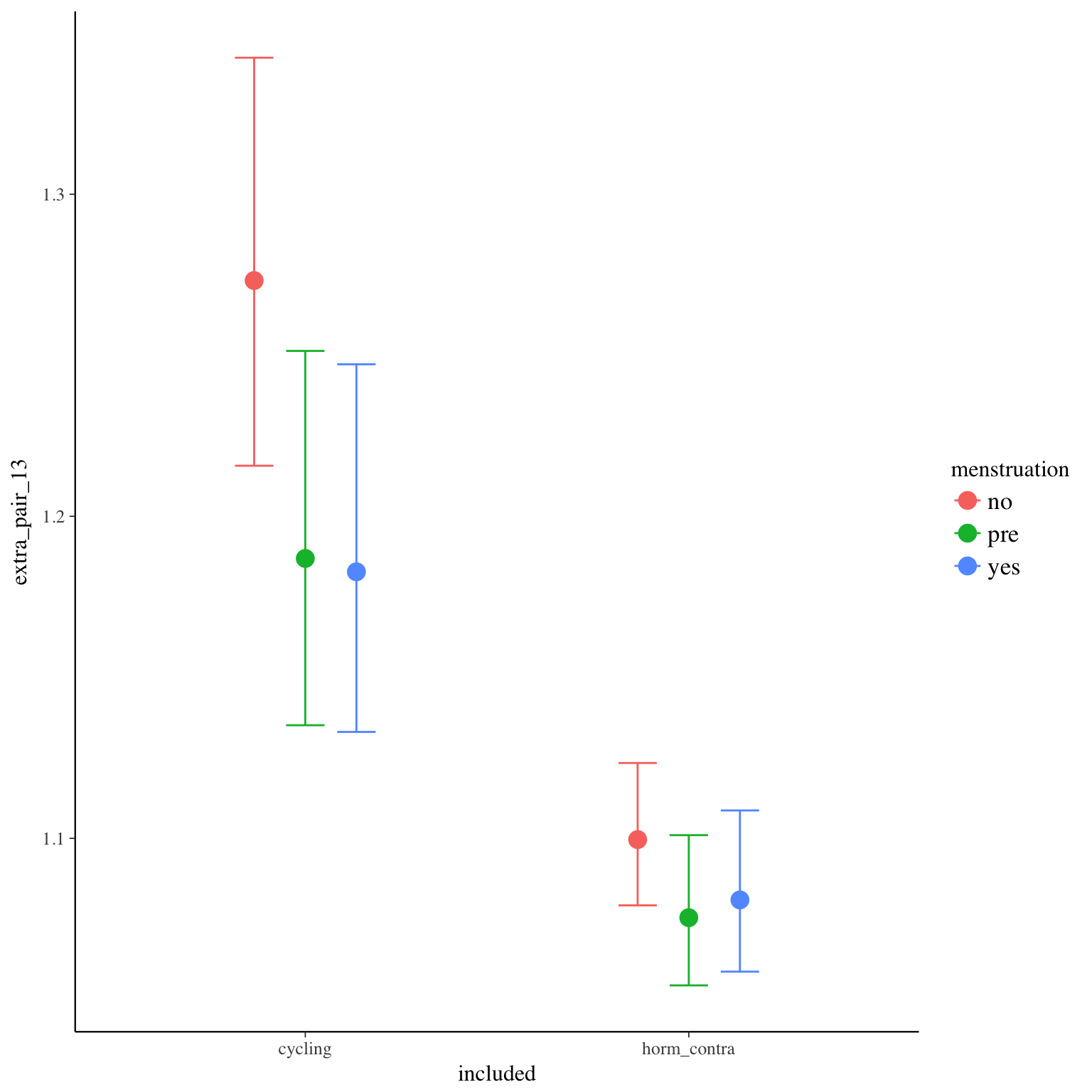
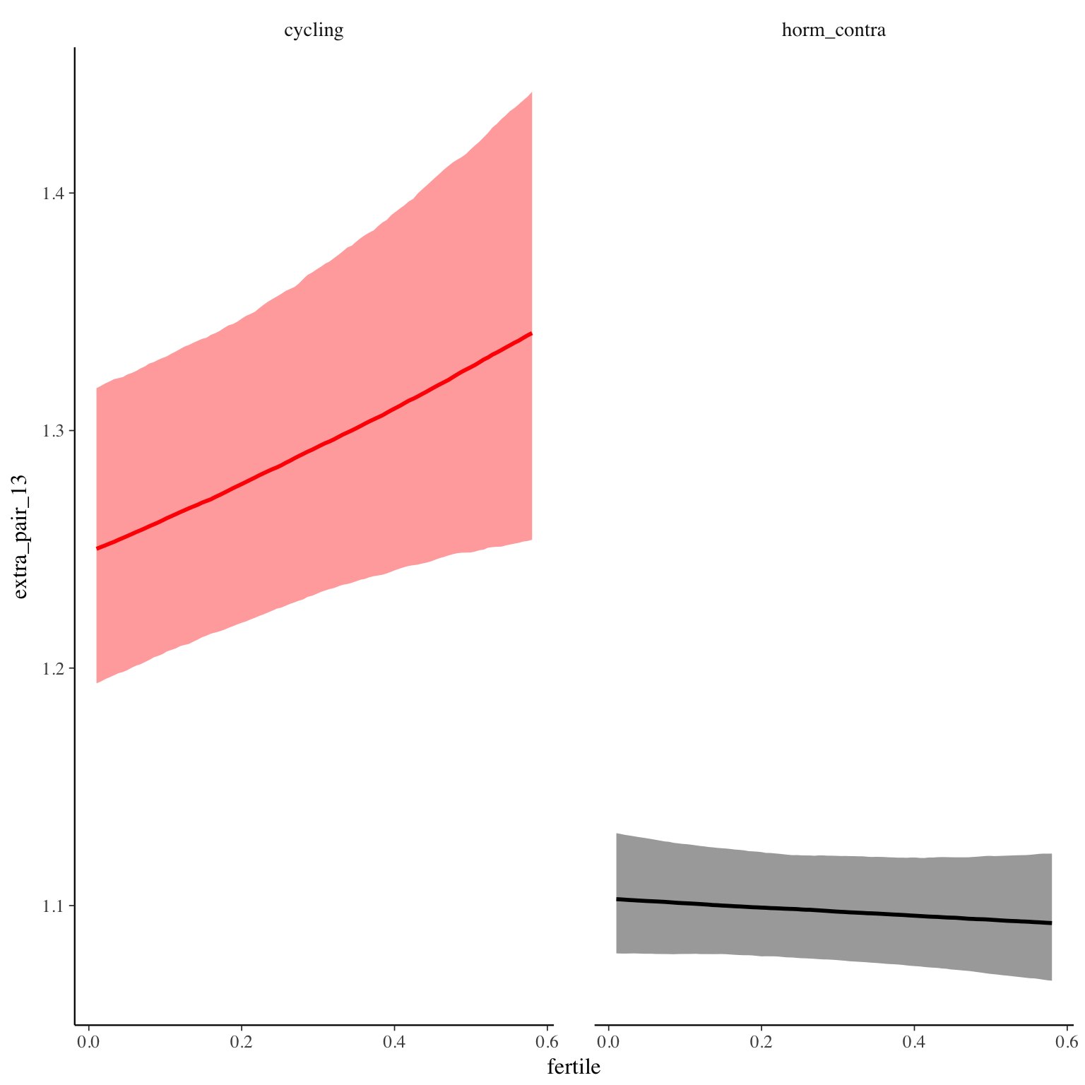
extra_pair_13
Item text:
… hatte ich sexuelle Fantasien mit anderen Männern als meinem Partner.
Item translation:
57. I had sexual fantasies about men other than my partner.
Choices:
| choice | value | frequency | percent |
|---|---|---|---|
| 1 | Stimme nicht zu | 24682 | 0.83 |
| 2 | Stimme überwiegend nicht zu | 1332 | 0.04 |
| 3 | Stimme eher nicht zu | 930 | 0.03 |
| 4 | Stimme eher zu | 1396 | 0.05 |
| 5 | Stimme überwiegend zu | 663 | 0.02 |
| 6 | Stimme voll zu | 870 | 0.03 |

Model
Model summary
Family: cumulative(logit)
Formula: extra_pair_13 ~ included * (menstruation + fertile) + fertile_mean + (1 + fertile + menstruation | person)
disc = 1
Data: diary (Number of observations: 26544)
Samples: 4 chains, each with iter = 2000; warmup = 1000; thin = 1;
total post-warmup samples = 4000
ICs: LOO = 29462.48; WAIC = Not computed
Group-Level Effects:
~person (Number of levels: 1043)
Estimate Est.Error l-95% CI u-95% CI Eff.Sample Rhat
sd(Intercept) 2.32 0.10 2.14 2.51 730 1.00
sd(fertile) 2.02 0.20 1.64 2.41 564 1.00
sd(menstruationpre) 0.88 0.12 0.65 1.11 505 1.01
sd(menstruationyes) 0.79 0.11 0.58 1.00 547 1.01
cor(Intercept,fertile) -0.08 0.11 -0.28 0.13 1861 1.00
cor(Intercept,menstruationpre) -0.12 0.12 -0.36 0.12 1950 1.00
cor(fertile,menstruationpre) 0.35 0.13 0.05 0.58 592 1.00
cor(Intercept,menstruationyes) 0.00 0.13 -0.26 0.25 2053 1.00
cor(fertile,menstruationyes) 0.42 0.13 0.14 0.66 705 1.01
cor(menstruationpre,menstruationyes) 0.79 0.10 0.57 0.96 545 1.00
Population-Level Effects:
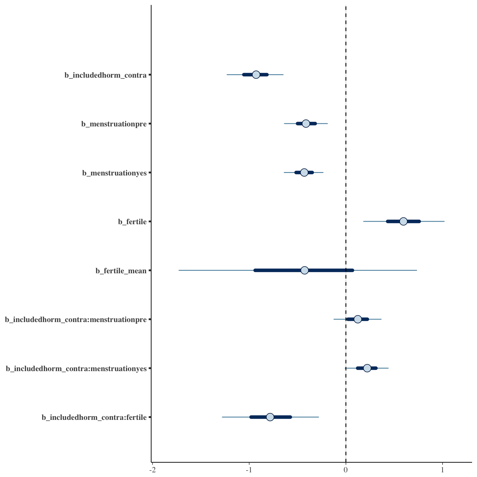
Estimate Est.Error l-95% CI u-95% CI Eff.Sample Rhat
Intercept[1] 1.97 0.19 1.61 2.34 952 1
Intercept[2] 2.54 0.19 2.18 2.92 960 1
Intercept[3] 3.02 0.19 2.65 3.39 913 1
Intercept[4] 4.04 0.19 3.67 4.41 918 1
Intercept[5] 4.86 0.19 4.49 5.24 937 1
includedhorm_contra -0.93 0.18 -1.28 -0.60 740 1
menstruationpre -0.41 0.13 -0.68 -0.15 2175 1
menstruationyes -0.43 0.12 -0.67 -0.20 2203 1
fertile 0.60 0.25 0.10 1.09 2223 1
fertile_mean -0.45 0.75 -2.00 0.94 1608 1
includedhorm_contra:menstruationpre 0.12 0.15 -0.17 0.41 2524 1
includedhorm_contra:menstruationyes 0.22 0.14 -0.06 0.48 2653 1
includedhorm_contra:fertile -0.78 0.30 -1.36 -0.21 2293 1
Samples were drawn using sampling(NUTS). For each parameter, Eff.Sample
is a crude measure of effective sample size, and Rhat is the potential
scale reduction factor on split chains (at convergence, Rhat = 1).
Coefficient plot
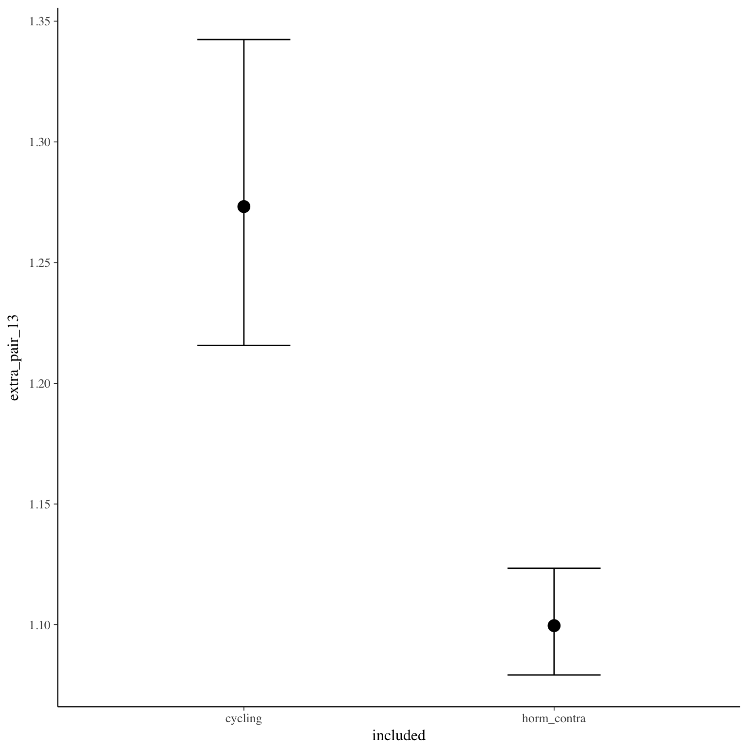
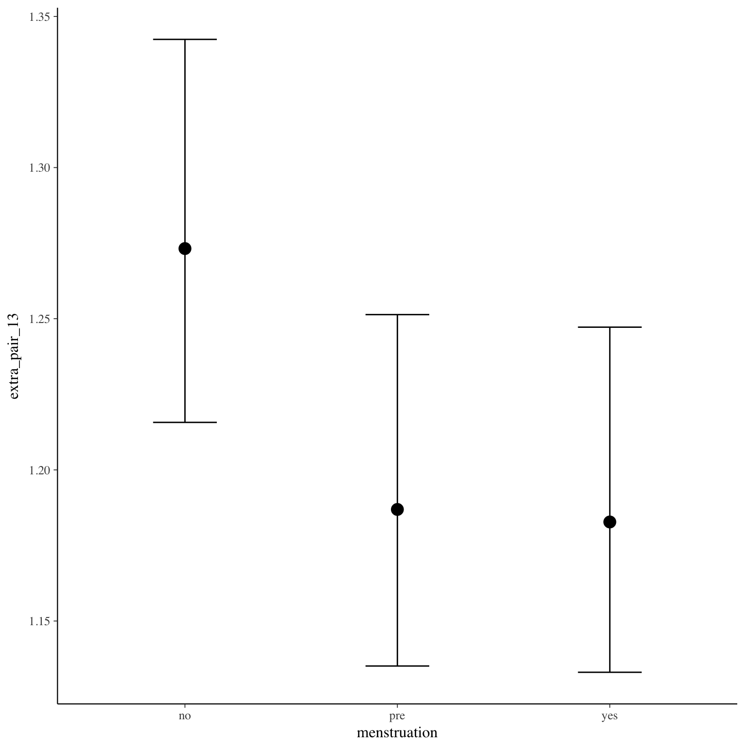
Marginal effect plots
Diagnostics

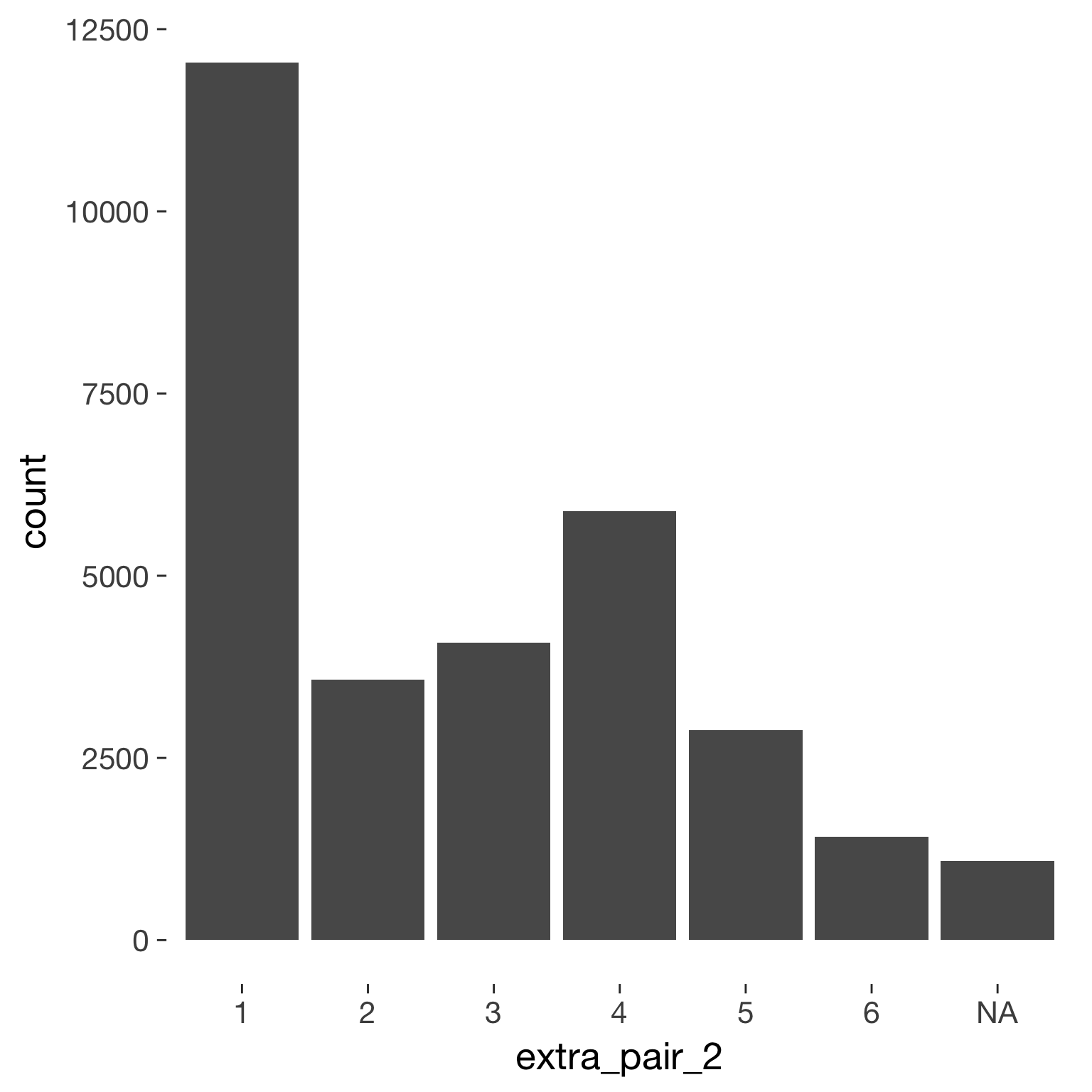
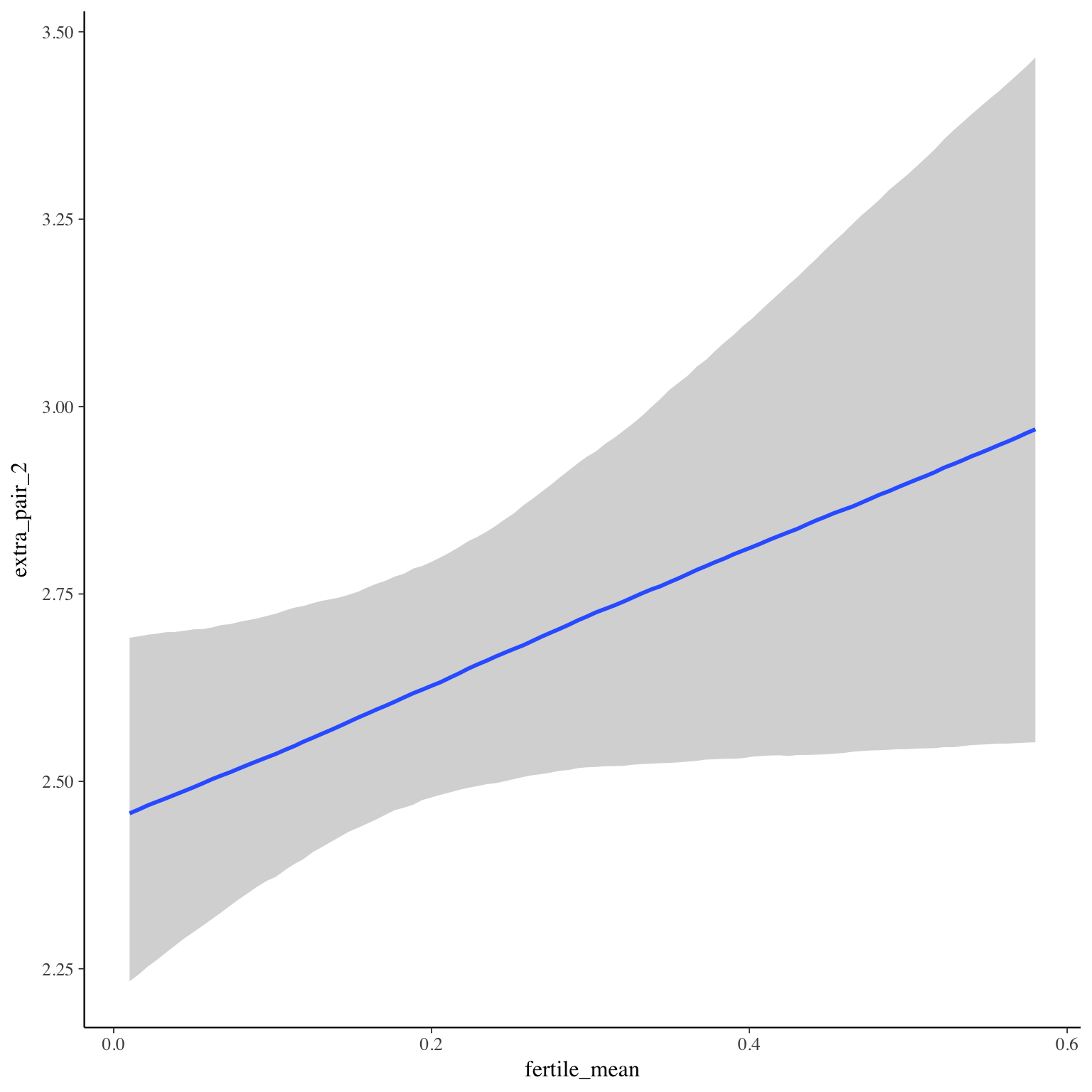
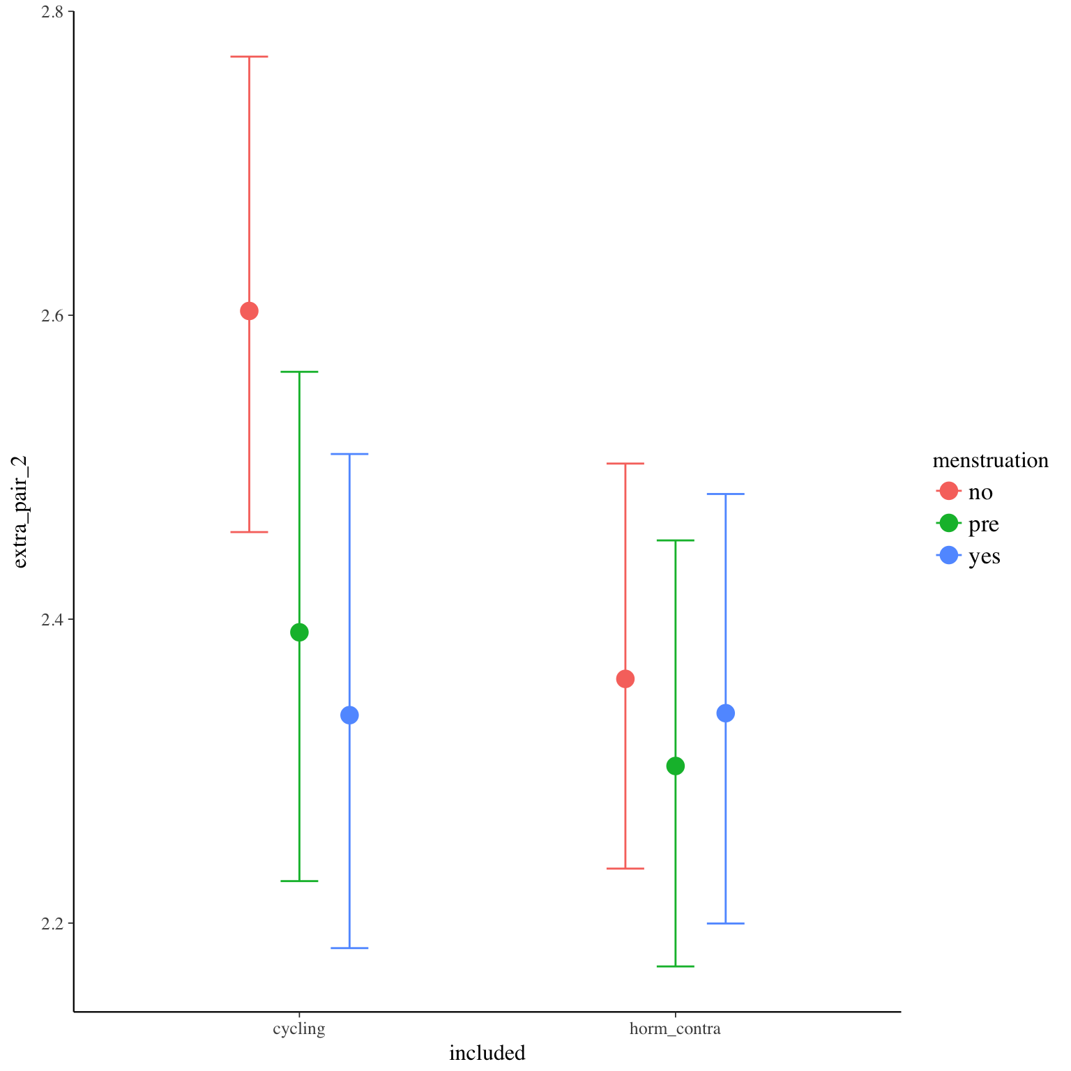
extra_pair_2
Item text:
…war es mir wichtig, dass mich andere Männer als attraktiv wahrnehmen.
Item translation:
46. It was important to me that other men perceive me to be attractive.
Choices:
| choice | value | frequency | percent |
|---|---|---|---|
| 1 | Stimme nicht zu | 12039 | 0.4 |
| 2 | Stimme überwiegend nicht zu | 3570 | 0.12 |
| 3 | Stimme eher nicht zu | 4078 | 0.14 |
| 4 | Stimme eher zu | 5888 | 0.2 |
| 5 | Stimme überwiegend zu | 2883 | 0.1 |
| 6 | Stimme voll zu | 1416 | 0.05 |
Model
Model summary
Family: cumulative(logit)
Formula: extra_pair_2 ~ included * (menstruation + fertile) + fertile_mean + (1 + fertile + menstruation | person)
disc = 1
Data: diary (Number of observations: 26544)
Samples: 4 chains, each with iter = 2000; warmup = 1000; thin = 1;
total post-warmup samples = 4000
ICs: LOO = 67203.83; WAIC = Not computed
Group-Level Effects:
~person (Number of levels: 1043)
Estimate Est.Error l-95% CI u-95% CI Eff.Sample Rhat
sd(Intercept) 2.18 0.06 2.06 2.32 716 1.01
sd(fertile) 1.64 0.13 1.38 1.89 529 1.01
sd(menstruationpre) 0.57 0.07 0.42 0.71 492 1.00
sd(menstruationyes) 0.77 0.06 0.65 0.90 867 1.00
cor(Intercept,fertile) -0.13 0.07 -0.28 0.01 2082 1.00
cor(Intercept,menstruationpre) -0.15 0.10 -0.34 0.06 2079 1.00
cor(fertile,menstruationpre) 0.44 0.11 0.21 0.63 593 1.00
cor(Intercept,menstruationyes) -0.26 0.08 -0.41 -0.11 2012 1.00
cor(fertile,menstruationyes) 0.48 0.09 0.29 0.65 581 1.01
cor(menstruationpre,menstruationyes) 0.79 0.09 0.59 0.95 192 1.04
Population-Level Effects:
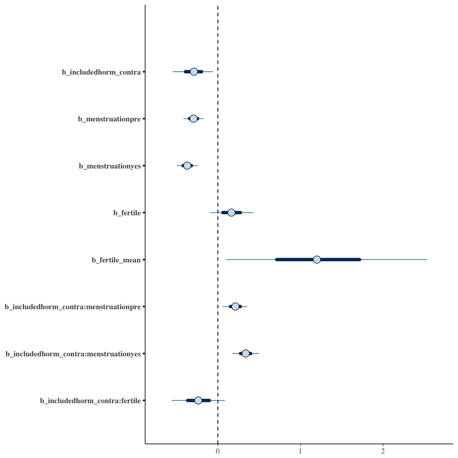
Estimate Est.Error l-95% CI u-95% CI Eff.Sample Rhat
Intercept[1] -0.67 0.17 -1.00 -0.34 448 1.00
Intercept[2] 0.17 0.17 -0.16 0.51 445 1.00
Intercept[3] 1.13 0.17 0.80 1.47 444 1.00
Intercept[4] 2.83 0.17 2.50 3.17 446 1.01
Intercept[5] 4.49 0.17 4.16 4.83 459 1.01
includedhorm_contra -0.29 0.15 -0.59 -0.01 291 1.01
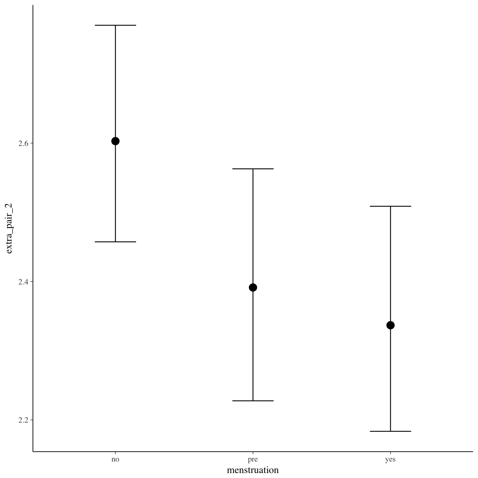
menstruationpre -0.29 0.07 -0.44 -0.15 1710 1.00
menstruationyes -0.37 0.07 -0.52 -0.23 1527 1.00
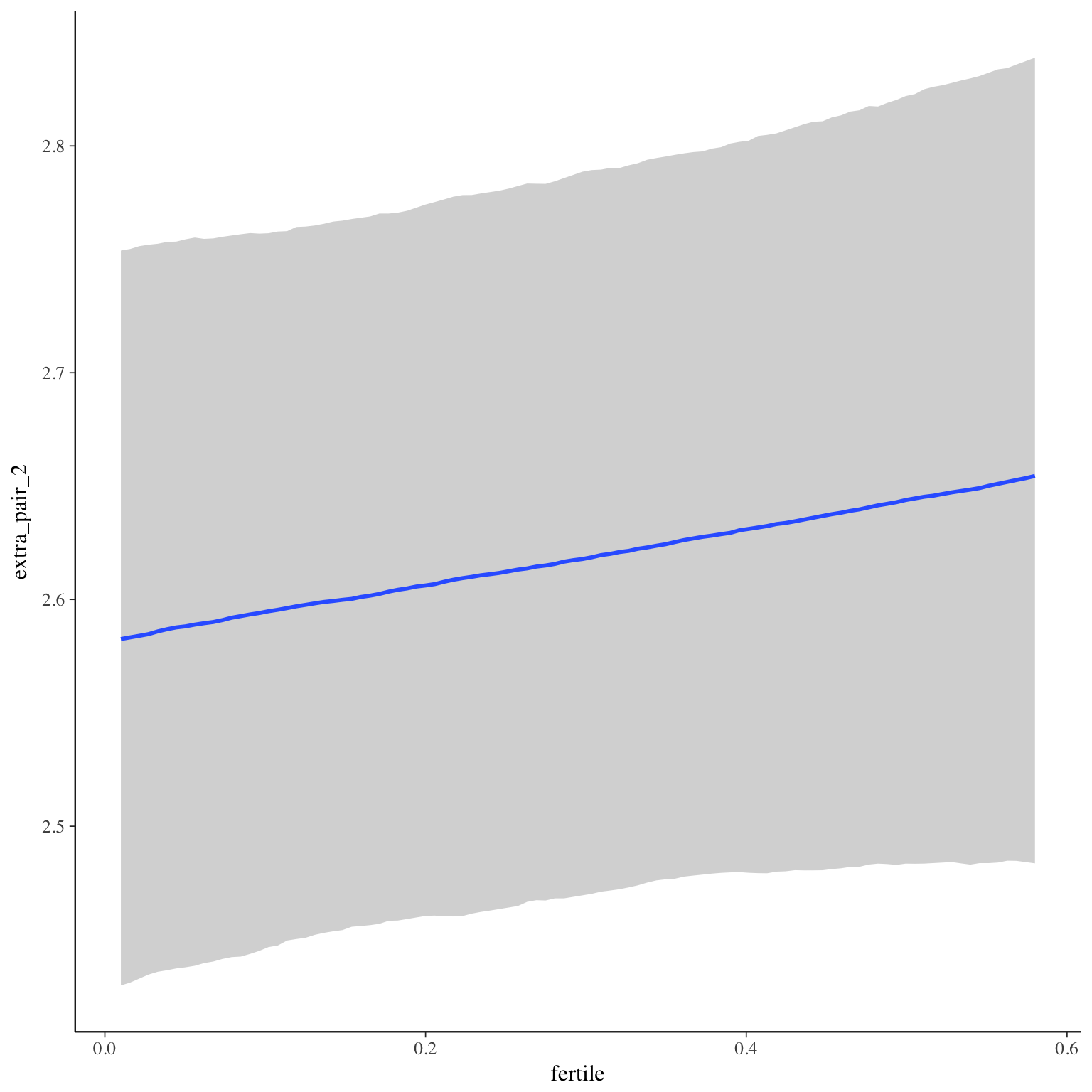
fertile 0.17 0.16 -0.14 0.47 1499 1.00
fertile_mean 1.23 0.74 -0.06 2.80 594 1.00
includedhorm_contra:menstruationpre 0.21 0.09 0.03 0.38 1733 1.00
includedhorm_contra:menstruationyes 0.34 0.09 0.16 0.53 1571 1.00
includedhorm_contra:fertile -0.24 0.20 -0.62 0.15 1518 1.00
Samples were drawn using sampling(NUTS). For each parameter, Eff.Sample
is a crude measure of effective sample size, and Rhat is the potential
scale reduction factor on split chains (at convergence, Rhat = 1).
Coefficient plot
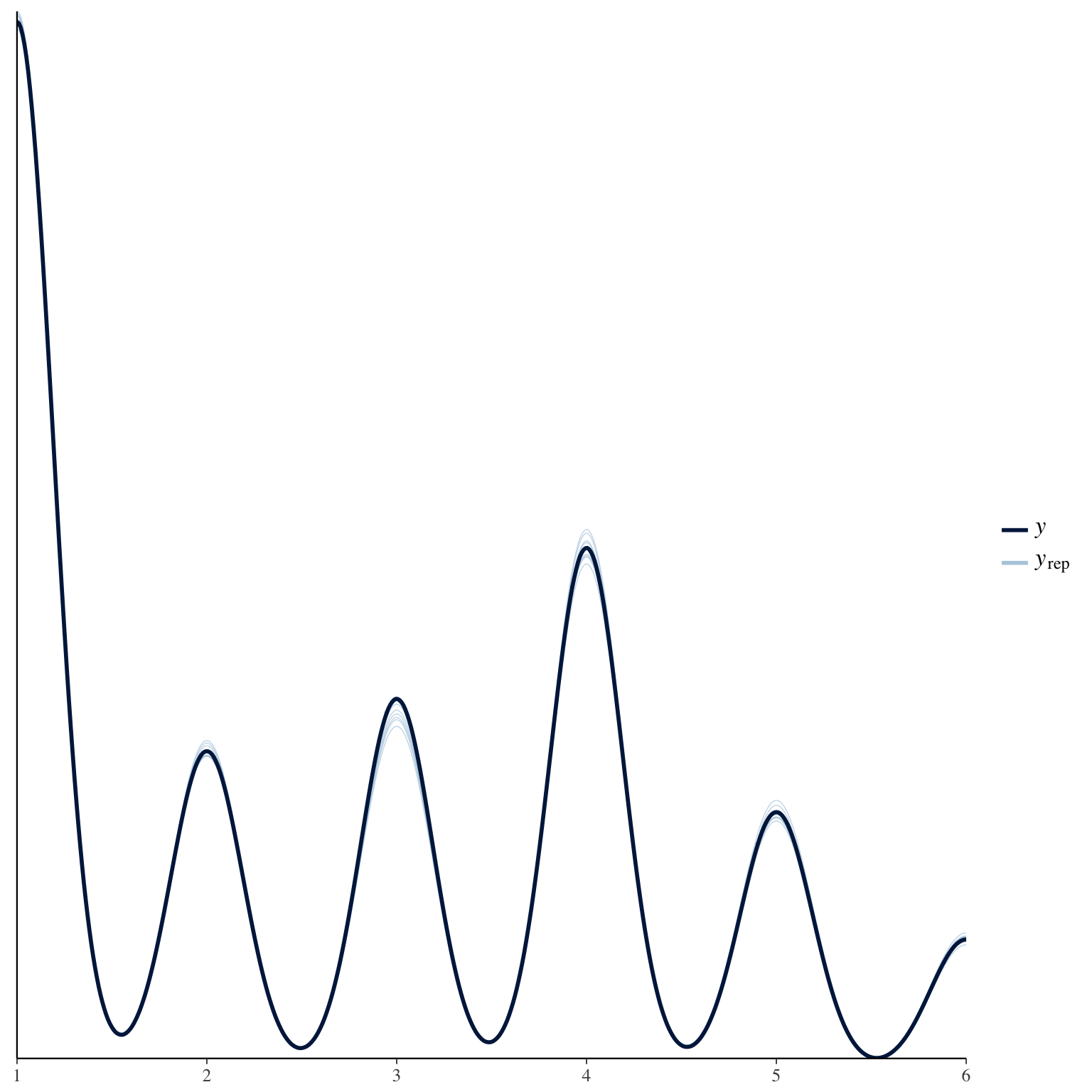
Marginal effect plots


Diagnostics
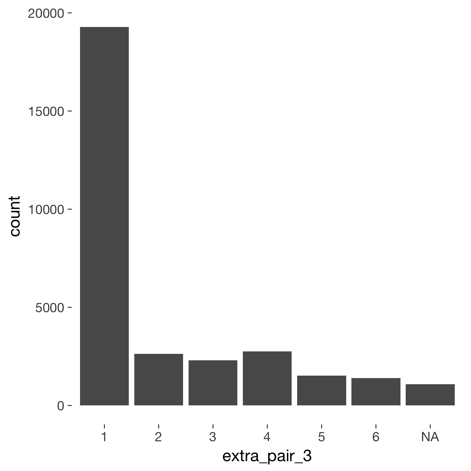
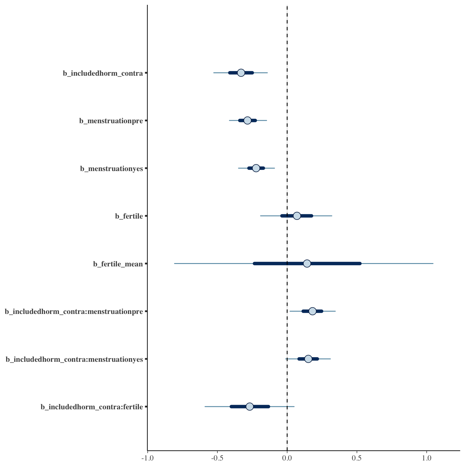
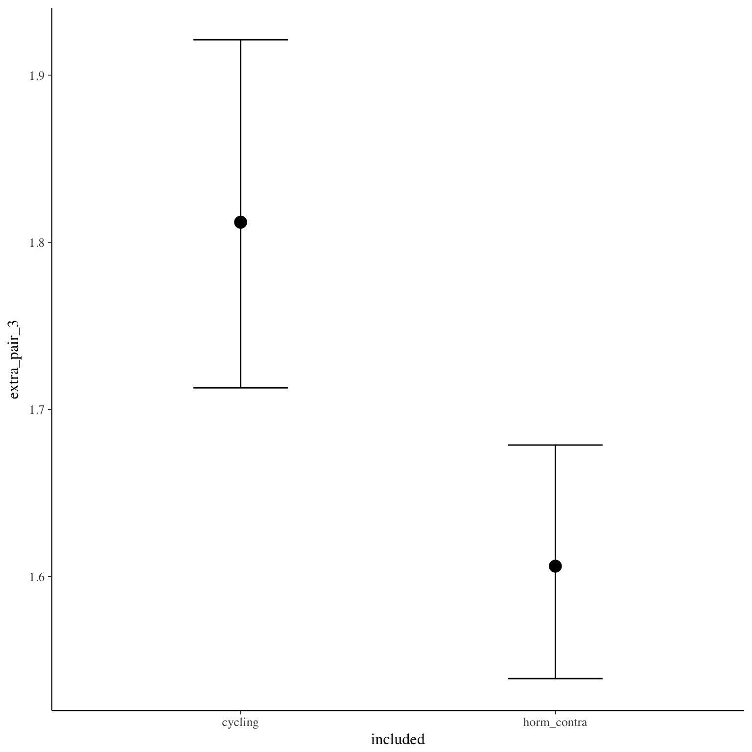
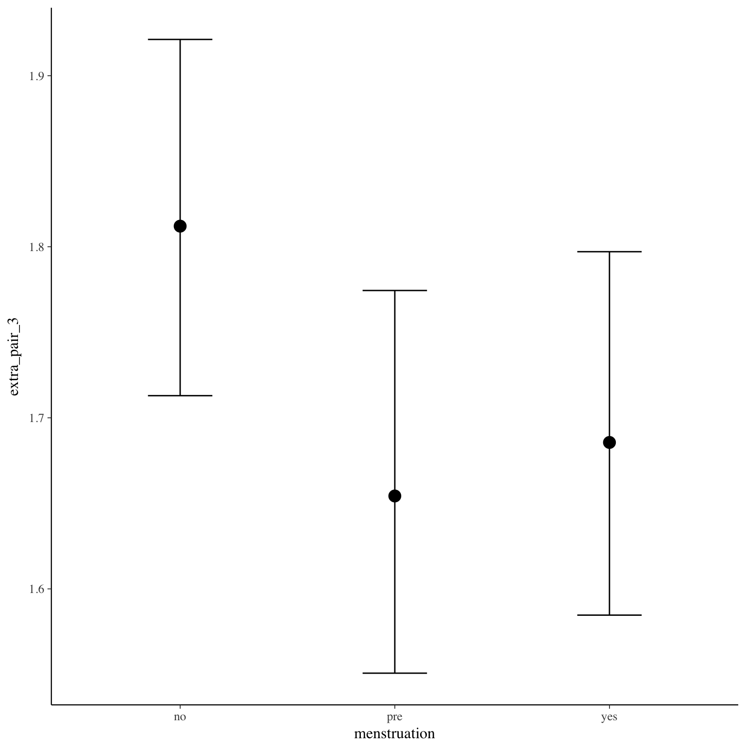
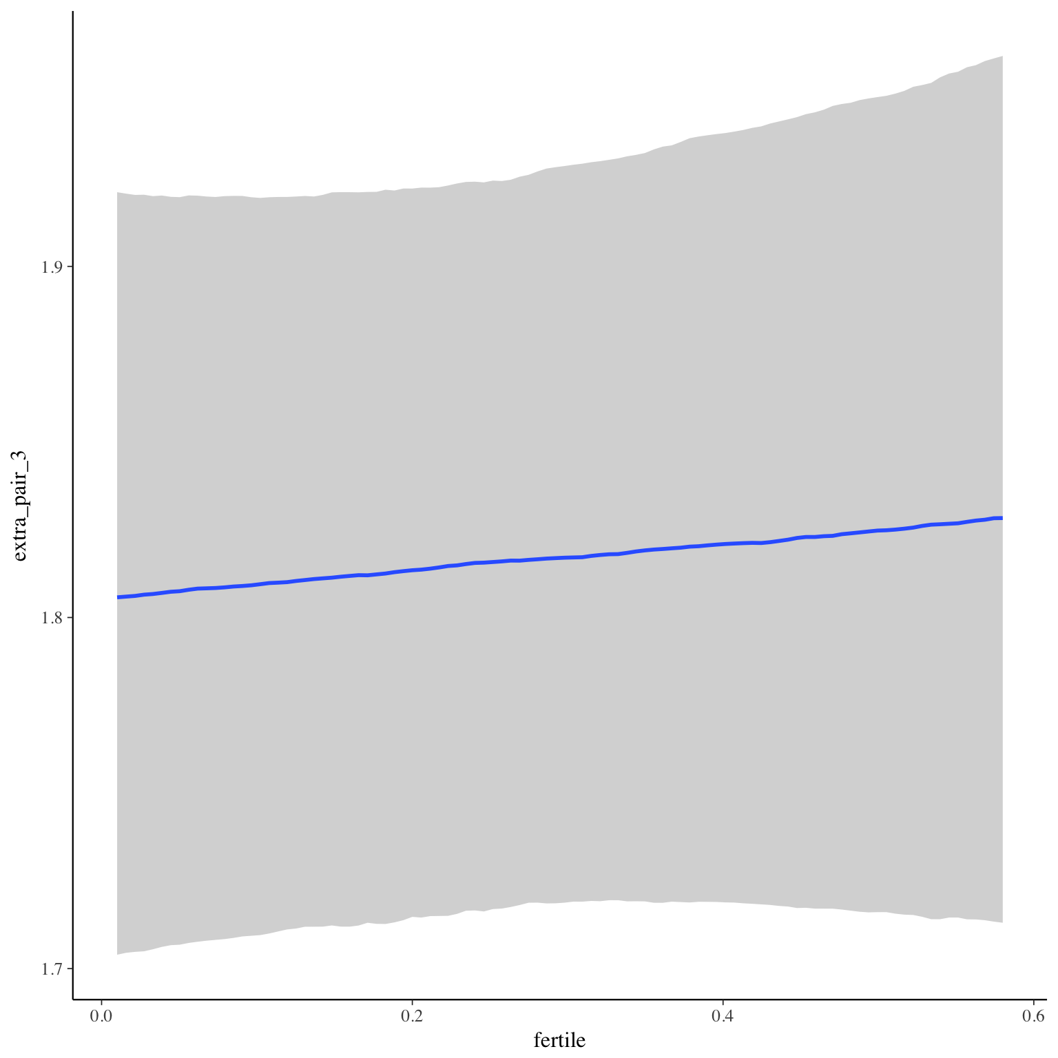
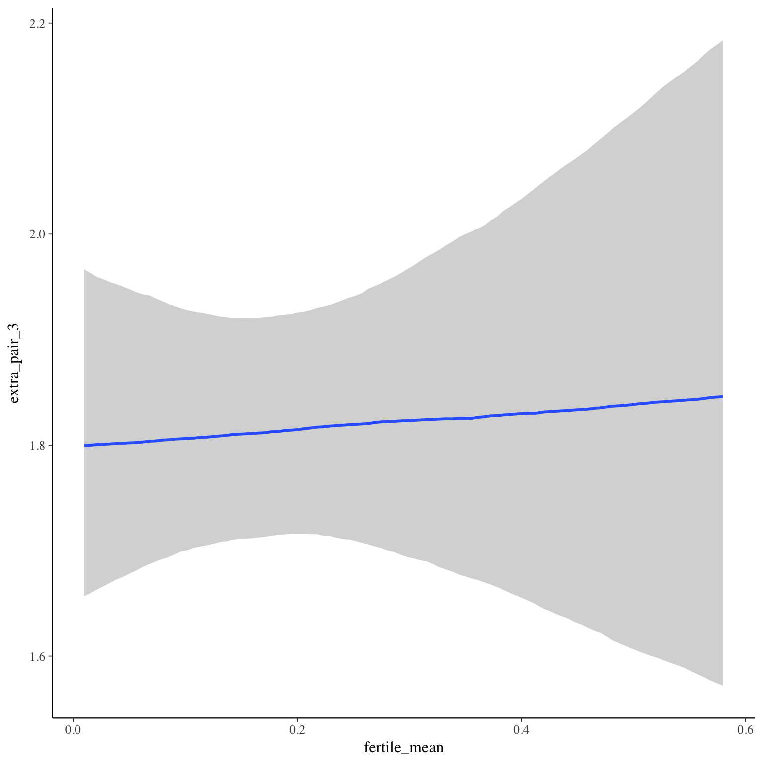
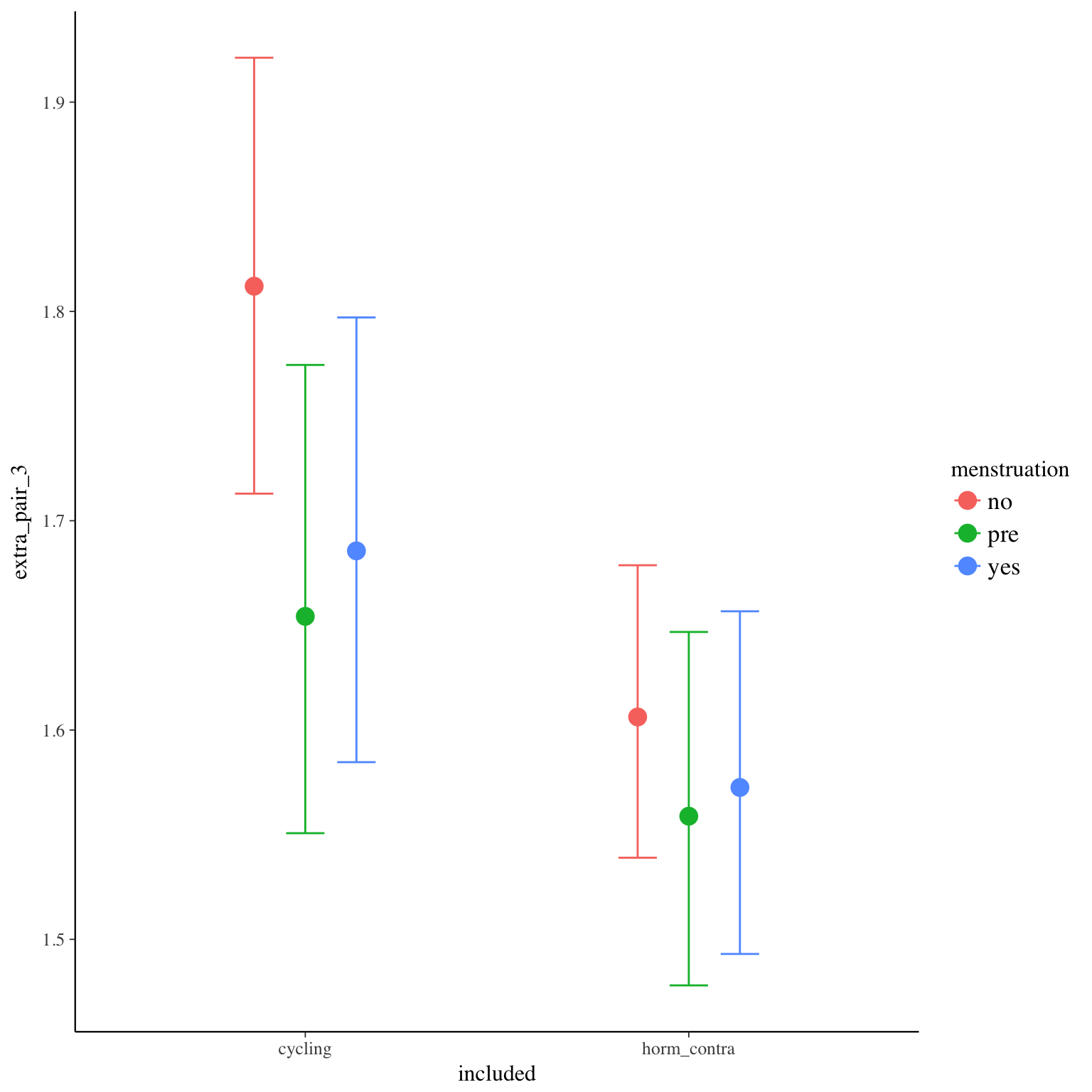
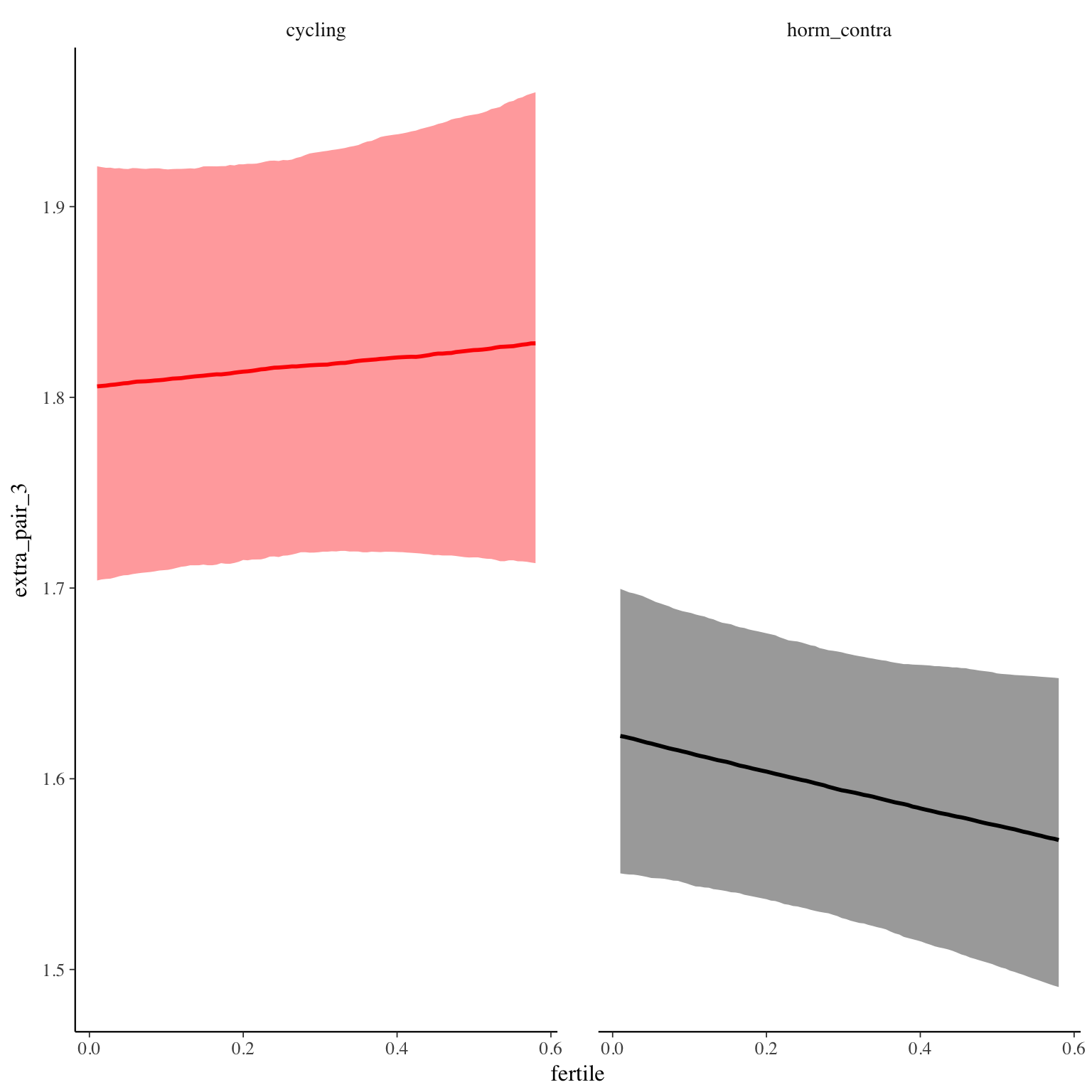
extra_pair_3
Item text:
… habe ich Komplimente von anderen Männern erhalten.
Item translation:
47. I received compliments from other men.
Choices:
| choice | value | frequency | percent |
|---|---|---|---|
| 1 | Stimme nicht zu | 19277 | 0.65 |
| 2 | Stimme überwiegend nicht zu | 2631 | 0.09 |
| 3 | Stimme eher nicht zu | 2303 | 0.08 |
| 4 | Stimme eher zu | 2754 | 0.09 |
| 5 | Stimme überwiegend zu | 1518 | 0.05 |
| 6 | Stimme voll zu | 1390 | 0.05 |
Model
Model summary
 Family: cumulative(logit)
Formula: extra_pair_3 ~ included * (menstruation + fertile) + fertile_mean + (1 + fertile + menstruation | person)
         disc = 1
   Data: diary (Number of observations: 26544)
Samples: 4 chains, each with iter = 2000; warmup = 1000; thin = 1;
         total post-warmup samples = 4000
    ICs: LOO = 55308.76; WAIC = Not computed

Group-Level Effects:
~person (Number of levels: 1043)
                                     Estimate Est.Error l-95% CI u-95% CI Eff.Sample Rhat
sd(Intercept)                            1.57      0.06     1.46     1.68       1022 1.00
sd(fertile)                              1.13      0.20     0.69     1.48        192 1.02
sd(menstruationpre)                      0.53      0.09     0.34     0.70        211 1.01
sd(menstruationyes)                      0.62      0.08     0.45     0.77        330 1.00
cor(Intercept,fertile)                   0.01      0.13    -0.22     0.29        372 1.01
cor(Intercept,menstruationpre)           0.09      0.14    -0.16     0.37        365 1.01
cor(fertile,menstruationpre)             0.36      0.22    -0.17     0.70        123 1.02
cor(Intercept,menstruationyes)          -0.13      0.11    -0.34     0.08       1161 1.00
cor(fertile,menstruationyes)             0.36      0.20    -0.10     0.66        151 1.01
cor(menstruationpre,menstruationyes)     0.82      0.11     0.56     0.97        230 1.01

Population-Level Effects:
                                    Estimate Est.Error l-95% CI u-95% CI Eff.Sample Rhat
Intercept[1]                            0.63      0.14     0.36     0.89        791 1.01
Intercept[2]                            1.24      0.14     0.97     1.50        791 1.01
Intercept[3]                            1.83      0.14     1.56     2.10        795 1.01
Intercept[4]                            2.80      0.14     2.53     3.07        803 1.01
Intercept[5]                            3.74      0.14     3.46     4.01        827 1.01
includedhorm_contra                    -0.33      0.12    -0.56    -0.11        642 1.01
menstruationpre                        -0.28      0.08    -0.44    -0.12       1851 1.00
menstruationyes                        -0.22      0.08    -0.37    -0.06       1758 1.00
fertile                                 0.07      0.16    -0.24     0.37       1805 1.00
fertile_mean                            0.13      0.57    -0.99     1.22       1270 1.00
includedhorm_contra:menstruationpre     0.18      0.10    -0.02     0.38       2080 1.00
includedhorm_contra:menstruationyes     0.15      0.10    -0.04     0.34       1817 1.00
includedhorm_contra:fertile            -0.27      0.19    -0.64     0.11       1935 1.00

Samples were drawn using sampling(NUTS). For each parameter, Eff.Sample
is a crude measure of effective sample size, and Rhat is the potential
scale reduction factor on split chains (at convergence, Rhat = 1).
Coefficient plot
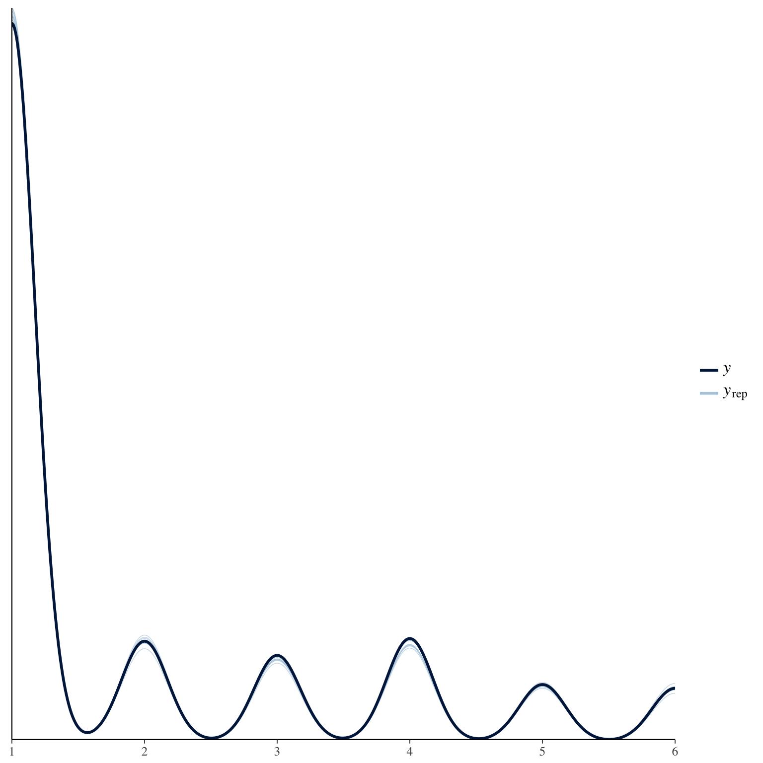
Marginal effect plots
Diagnostics
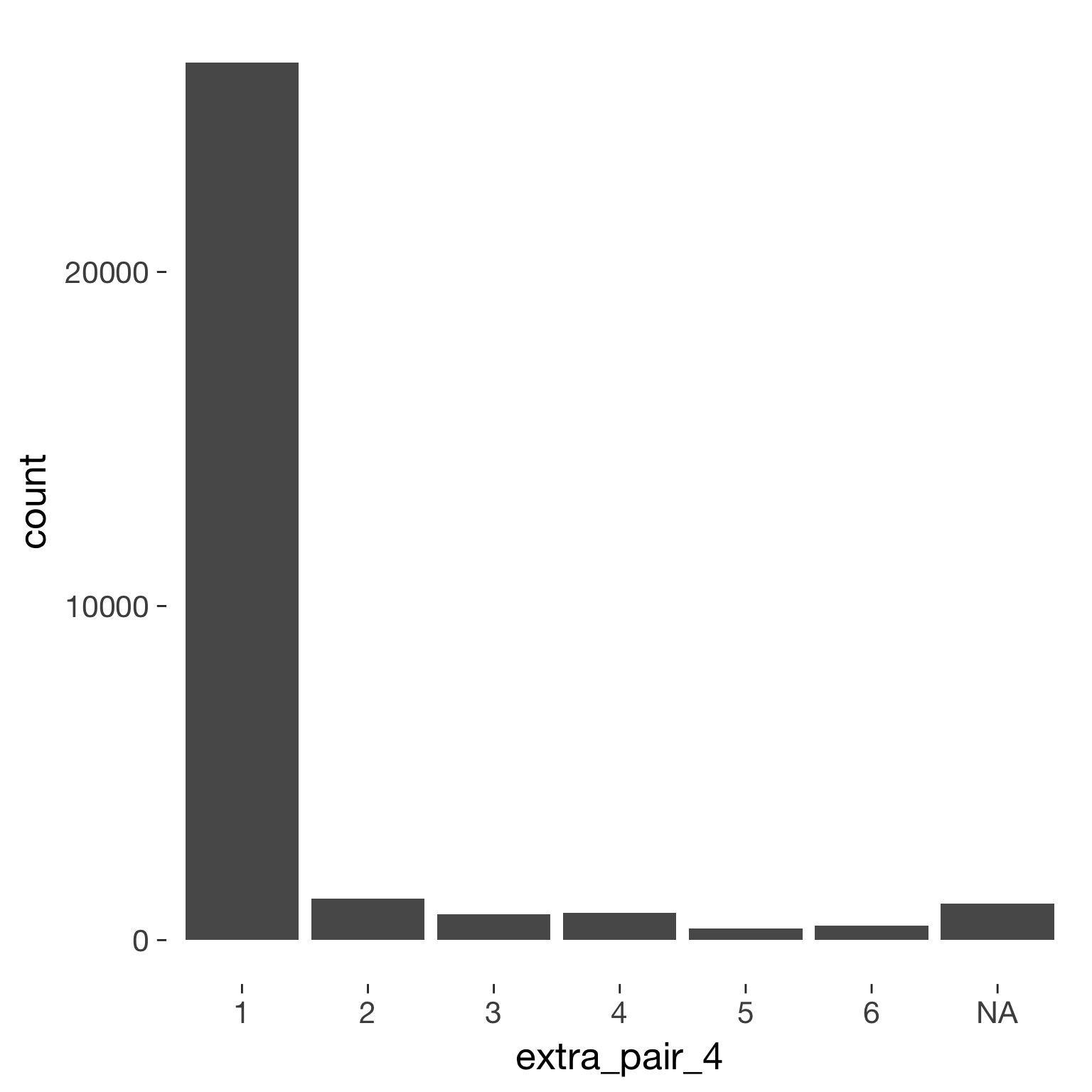
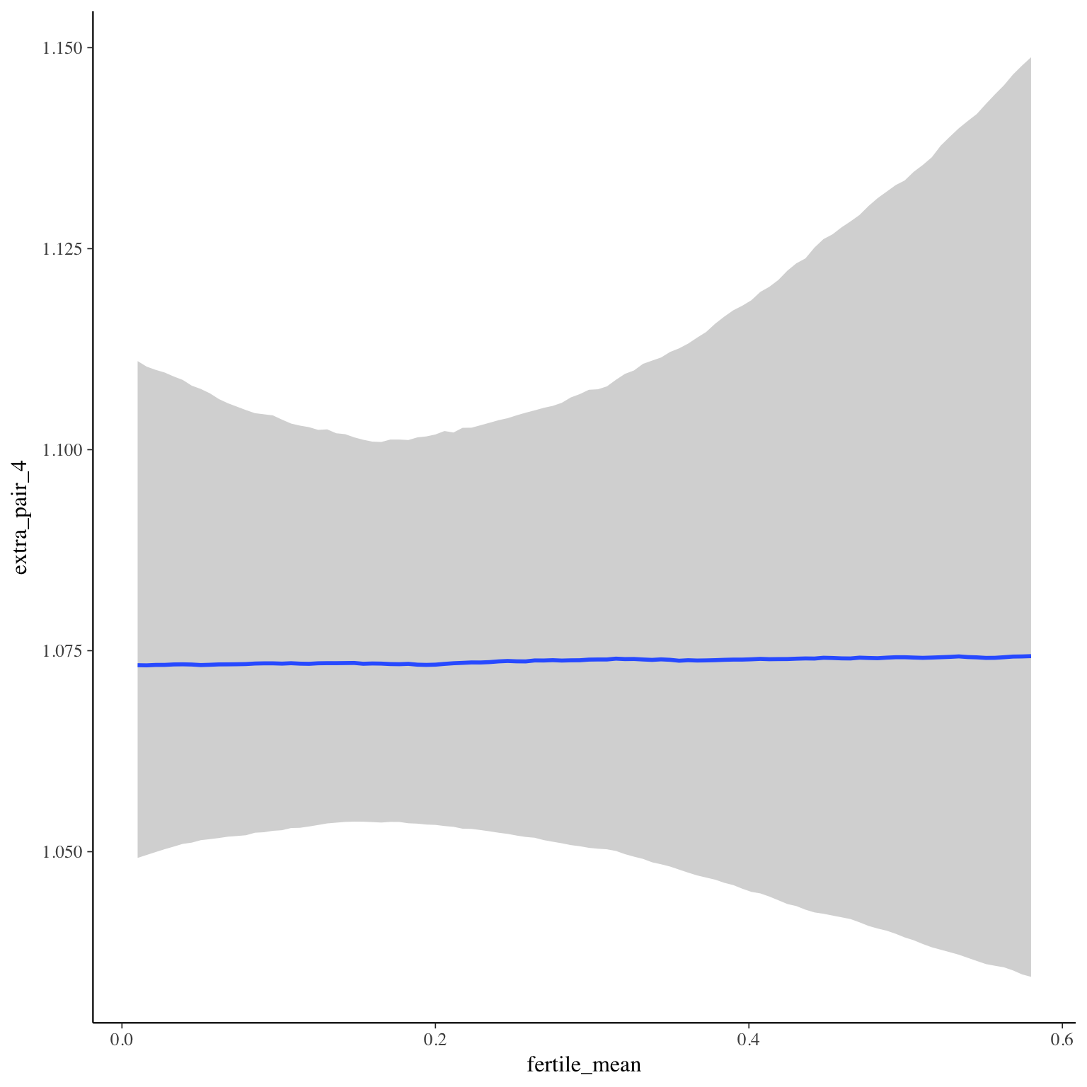
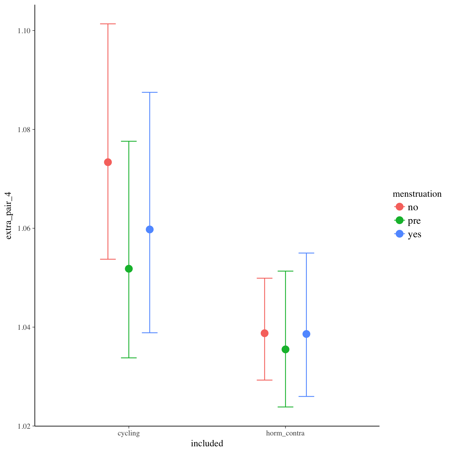
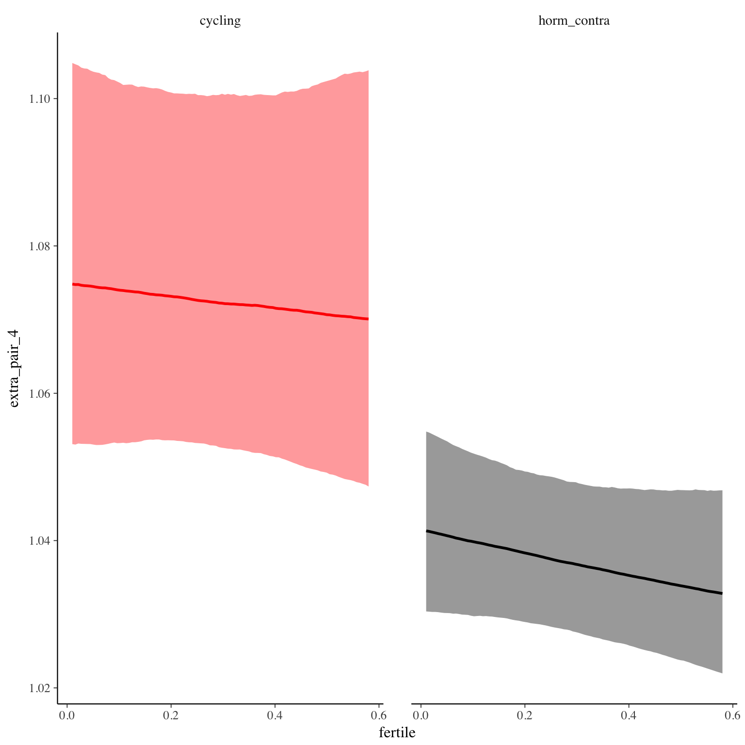
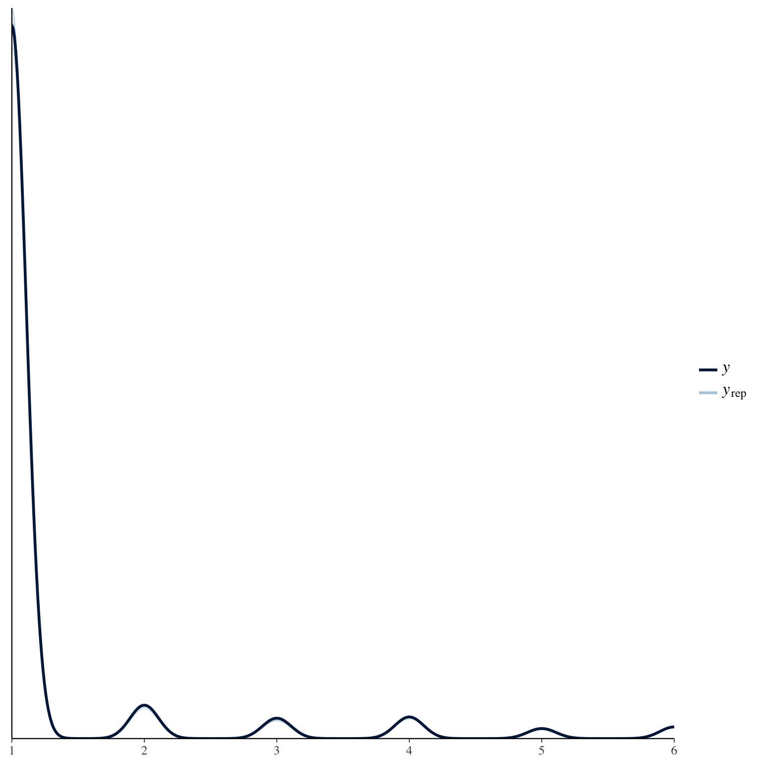
extra_pair_4
Item text:
… habe ich via Medien mit Freunden, Bekannten oder Kollegen geflirtet.
Item translation:
48. I flirted via media with friends, acquaintances, or colleagues.
Choices:
| choice | value | frequency | percent |
|---|---|---|---|
| 1 | Stimme nicht zu | 26262 | 0.88 |
| 2 | Stimme überwiegend nicht zu | 1237 | 0.04 |
| 3 | Stimme eher nicht zu | 763 | 0.03 |
| 4 | Stimme eher zu | 825 | 0.03 |
| 5 | Stimme überwiegend zu | 355 | 0.01 |
| 6 | Stimme voll zu | 431 | 0.01 |
Model
Model summary
Family: cumulative(logit)
Formula: extra_pair_4 ~ included * (menstruation + fertile) + fertile_mean + (1 + fertile + menstruation | person)
disc = 1
Data: diary (Number of observations: 26544)
Samples: 4 chains, each with iter = 2000; warmup = 1000; thin = 1;
total post-warmup samples = 4000
ICs: LOO = 21161.83; WAIC = Not computed
Group-Level Effects:
~person (Number of levels: 1043)
Estimate Est.Error l-95% CI u-95% CI Eff.Sample Rhat
sd(Intercept) 2.57 0.11 2.35 2.80 658 1.01
sd(fertile) 1.93 0.27 1.39 2.43 408 1.02
sd(menstruationpre) 0.82 0.13 0.55 1.08 501 1.01
sd(menstruationyes) 0.68 0.16 0.34 0.97 329 1.02
cor(Intercept,fertile) 0.00 0.14 -0.26 0.28 1331 1.01
cor(Intercept,menstruationpre) 0.03 0.15 -0.27 0.33 1174 1.00
cor(fertile,menstruationpre) 0.25 0.19 -0.16 0.57 333 1.02
cor(Intercept,menstruationyes) -0.04 0.18 -0.39 0.32 1475 1.00
cor(fertile,menstruationyes) 0.28 0.22 -0.24 0.63 255 1.02
cor(menstruationpre,menstruationyes) 0.72 0.16 0.36 0.96 590 1.00
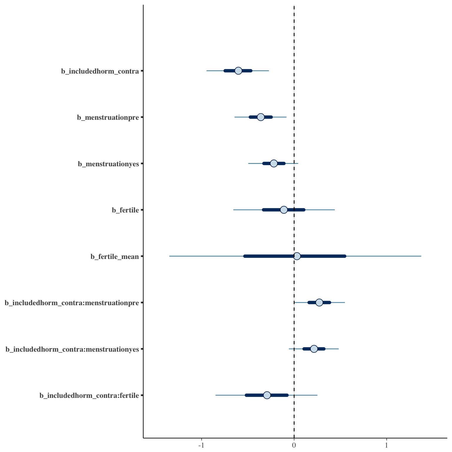
Population-Level Effects:
Estimate Est.Error l-95% CI u-95% CI Eff.Sample Rhat
Intercept[1] 3.18 0.23 2.73 3.63 590 1.01
Intercept[2] 3.94 0.23 3.48 4.39 598 1.01
Intercept[3] 4.55 0.23 4.09 5.01 614 1.01
Intercept[4] 5.56 0.24 5.10 6.02 617 1.01
Intercept[5] 6.44 0.24 5.96 6.91 635 1.01
includedhorm_contra -0.61 0.20 -1.01 -0.21 405 1.01
menstruationpre -0.36 0.17 -0.69 -0.04 1796 1.00
menstruationyes -0.22 0.16 -0.54 0.08 1333 1.01
fertile -0.11 0.33 -0.75 0.54 1707 1.00
fertile_mean 0.01 0.83 -1.69 1.64 1337 1.00
includedhorm_contra:menstruationpre 0.27 0.17 -0.06 0.60 2039 1.00
includedhorm_contra:menstruationyes 0.22 0.16 -0.10 0.53 2174 1.00
includedhorm_contra:fertile -0.30 0.33 -0.97 0.34 2136 1.00
Samples were drawn using sampling(NUTS). For each parameter, Eff.Sample
is a crude measure of effective sample size, and Rhat is the potential
scale reduction factor on split chains (at convergence, Rhat = 1).
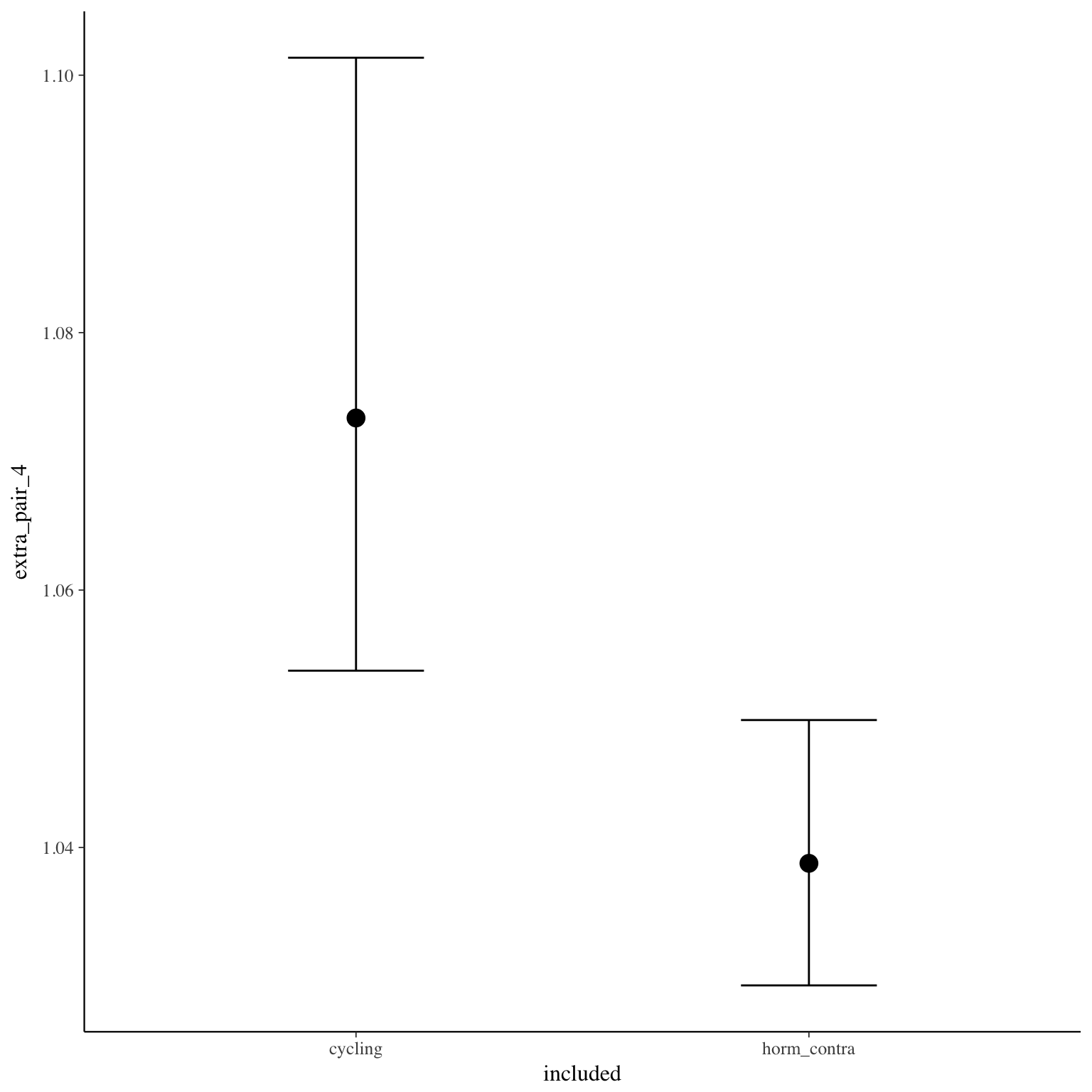
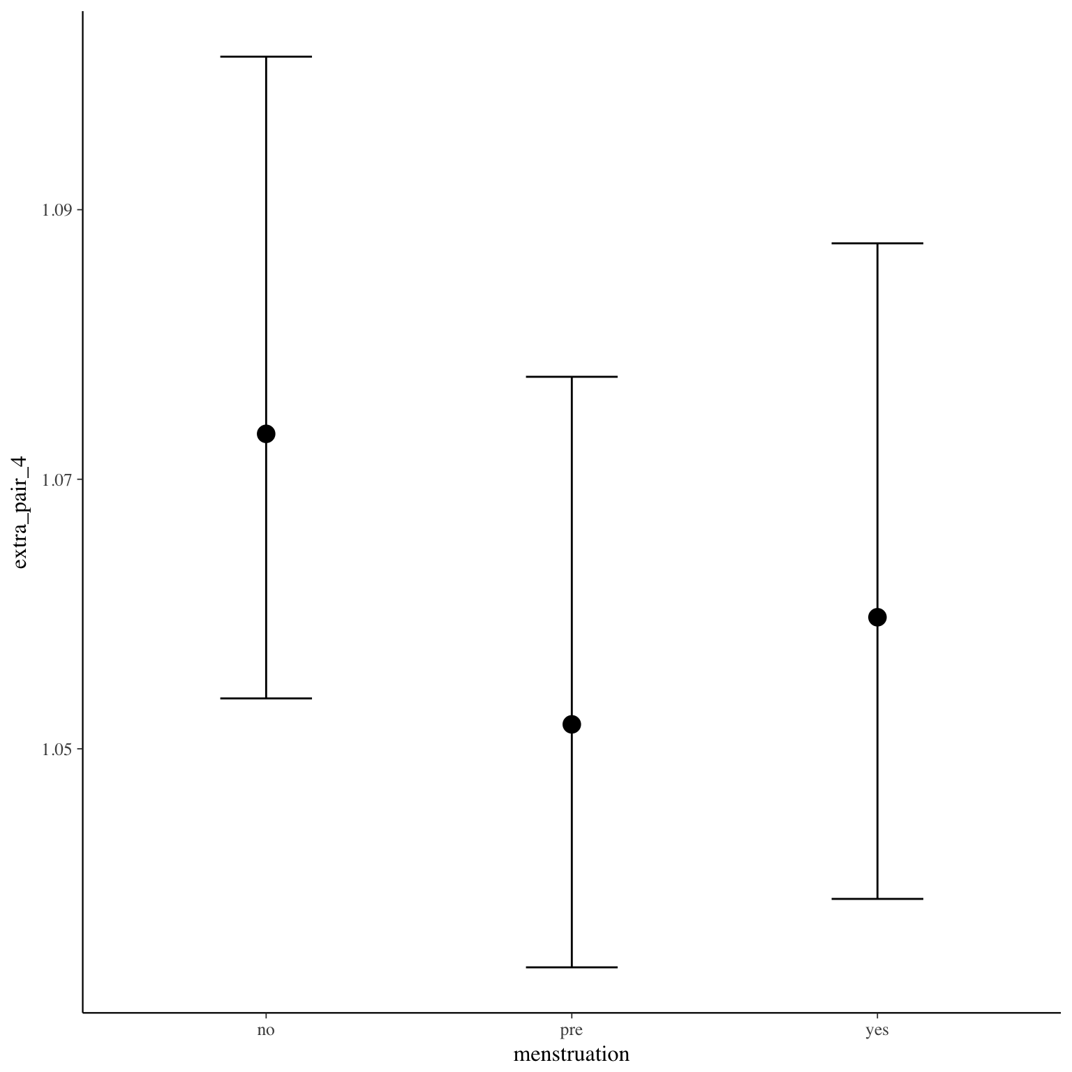
Coefficient plot
Marginal effect plots

Diagnostics
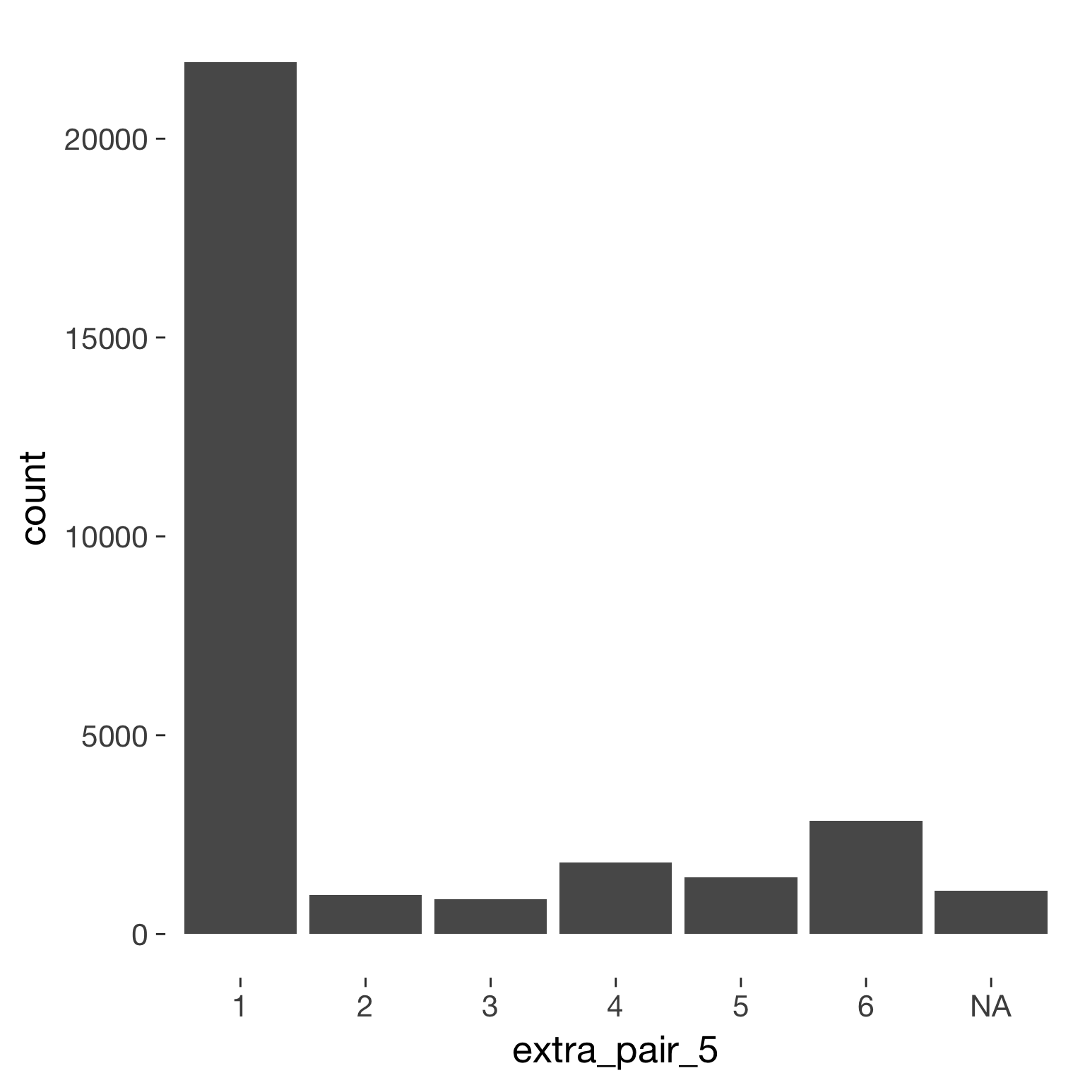
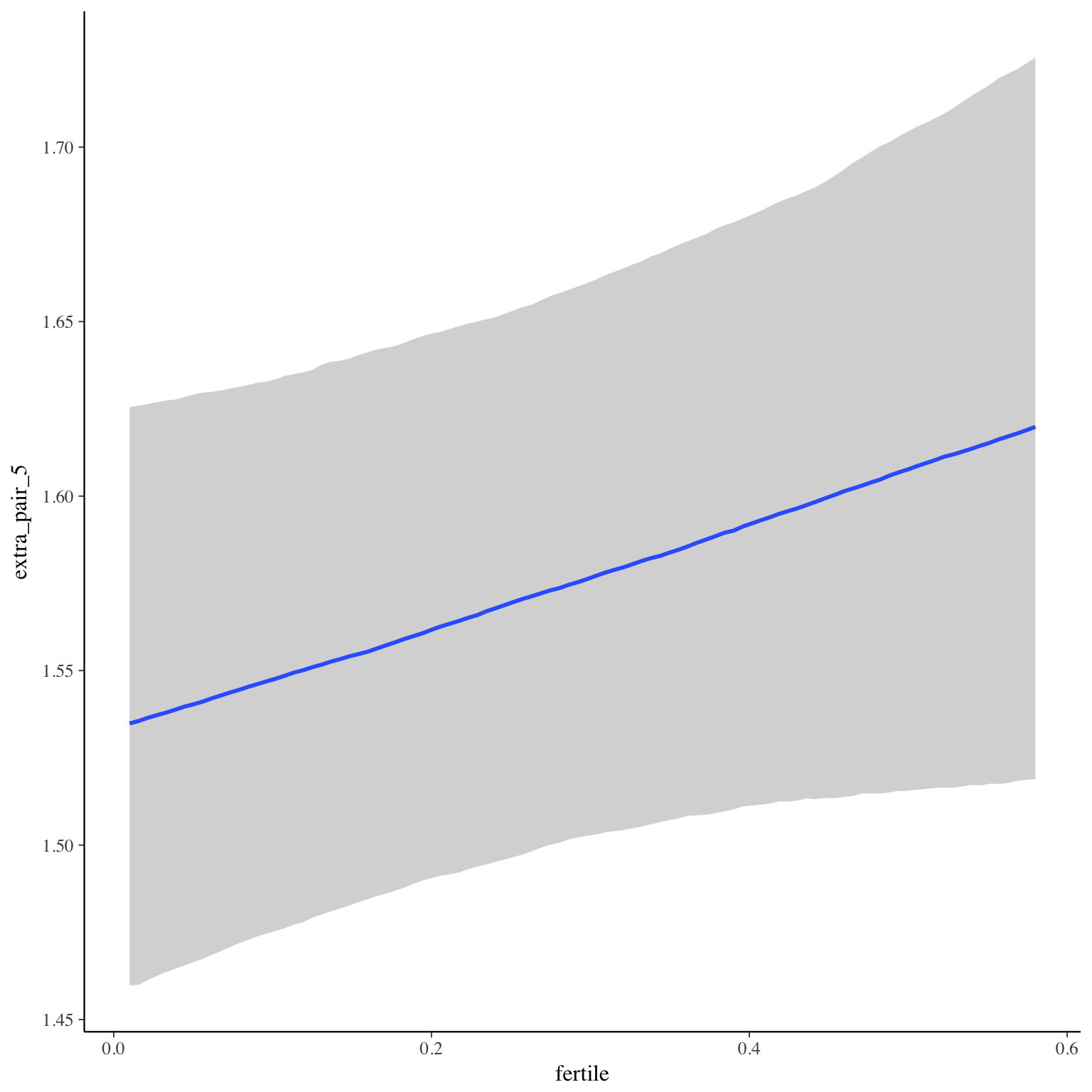
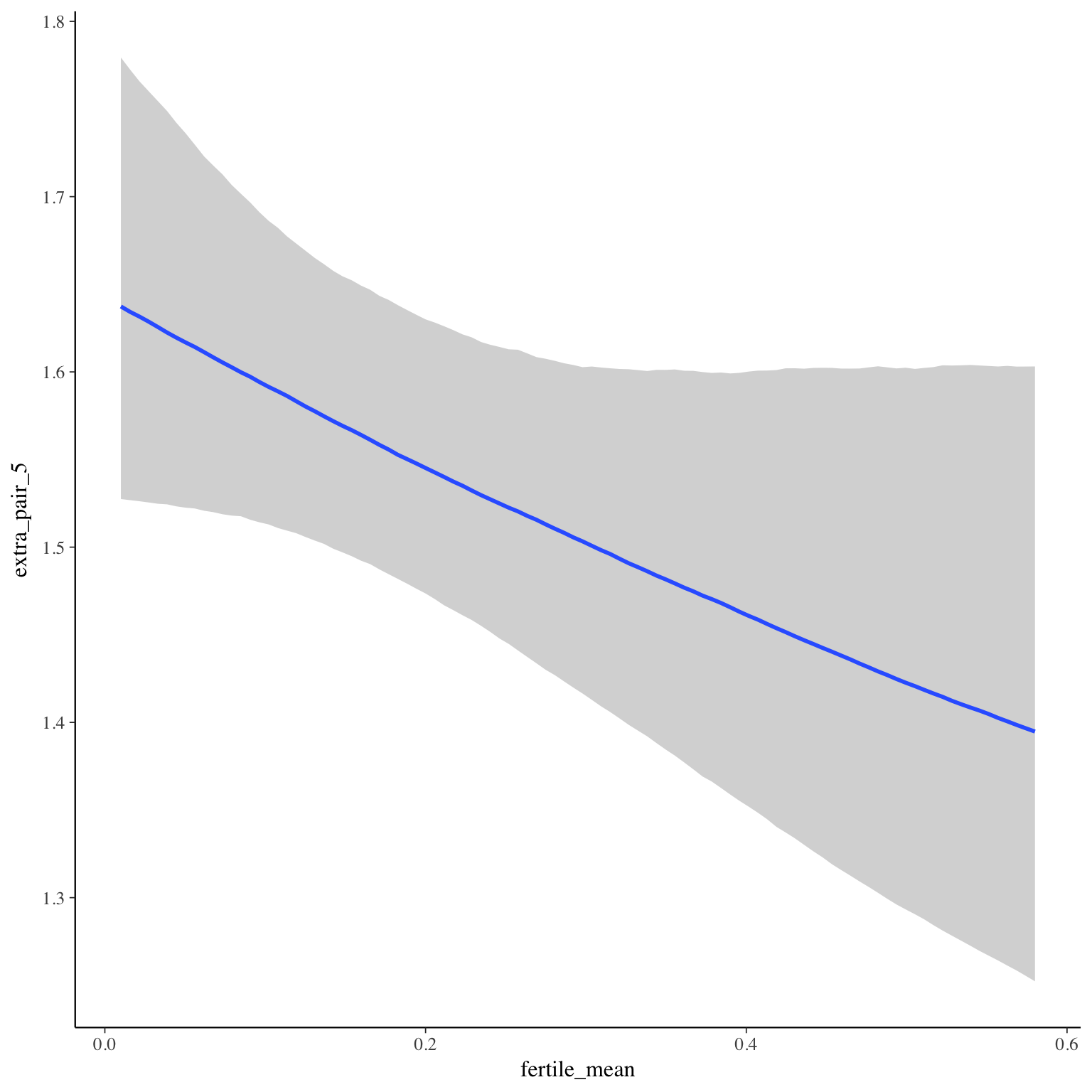
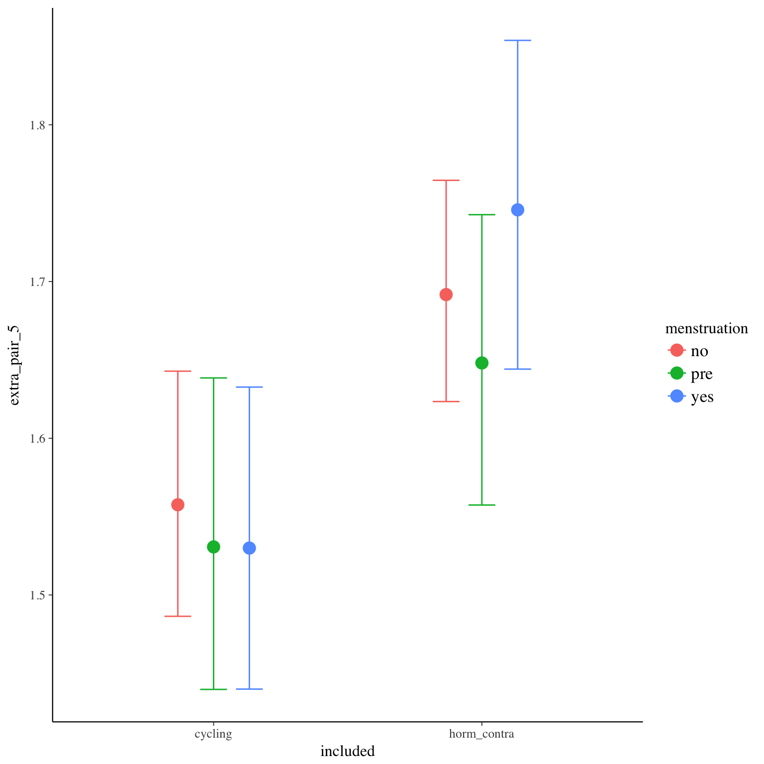
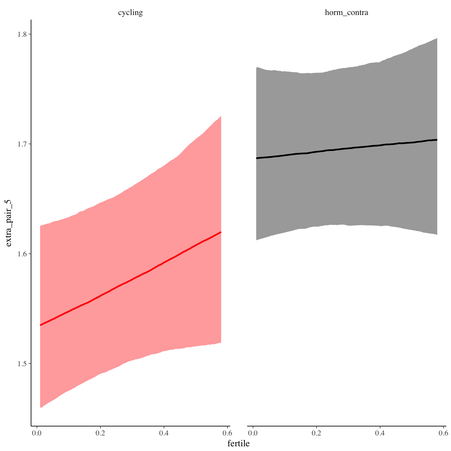
extra_pair_5
Item text:
… bin ich ohne meinen Partner ausgegangen.
Item translation:
51. I went out without my partner.
Choices:
| choice | value | frequency | percent |
|---|---|---|---|
| 1 | Stimme nicht zu | 21919 | 0.73 |
| 2 | Stimme überwiegend nicht zu | 991 | 0.03 |
| 3 | Stimme eher nicht zu | 877 | 0.03 |
| 4 | Stimme eher zu | 1804 | 0.06 |
| 5 | Stimme überwiegend zu | 1429 | 0.05 |
| 6 | Stimme voll zu | 2853 | 0.1 |
Model
Model summary
Family: cumulative(logit)
Formula: extra_pair_5 ~ included * (menstruation + fertile) + fertile_mean + (1 + fertile + menstruation | person)
disc = 1
Data: diary (Number of observations: 26544)
Samples: 4 chains, each with iter = 2000; warmup = 1000; thin = 1;
total post-warmup samples = 4000
ICs: LOO = 46661.05; WAIC = Not computed
Group-Level Effects:
~person (Number of levels: 1043)
Estimate Est.Error l-95% CI u-95% CI Eff.Sample Rhat
sd(Intercept) 1.33 0.05 1.23 1.44 832 1.01
sd(fertile) 1.16 0.20 0.74 1.54 250 1.02
sd(menstruationpre) 0.43 0.13 0.17 0.66 219 1.02
sd(menstruationyes) 0.67 0.09 0.49 0.84 420 1.02
cor(Intercept,fertile) -0.18 0.12 -0.40 0.08 802 1.01
cor(Intercept,menstruationpre) 0.10 0.19 -0.23 0.52 407 1.01
cor(fertile,menstruationpre) 0.17 0.29 -0.51 0.63 201 1.02
cor(Intercept,menstruationyes) -0.12 0.11 -0.33 0.11 643 1.01
cor(fertile,menstruationyes) 0.43 0.17 0.04 0.73 250 1.01
cor(menstruationpre,menstruationyes) 0.64 0.17 0.24 0.91 268 1.01
Population-Level Effects:
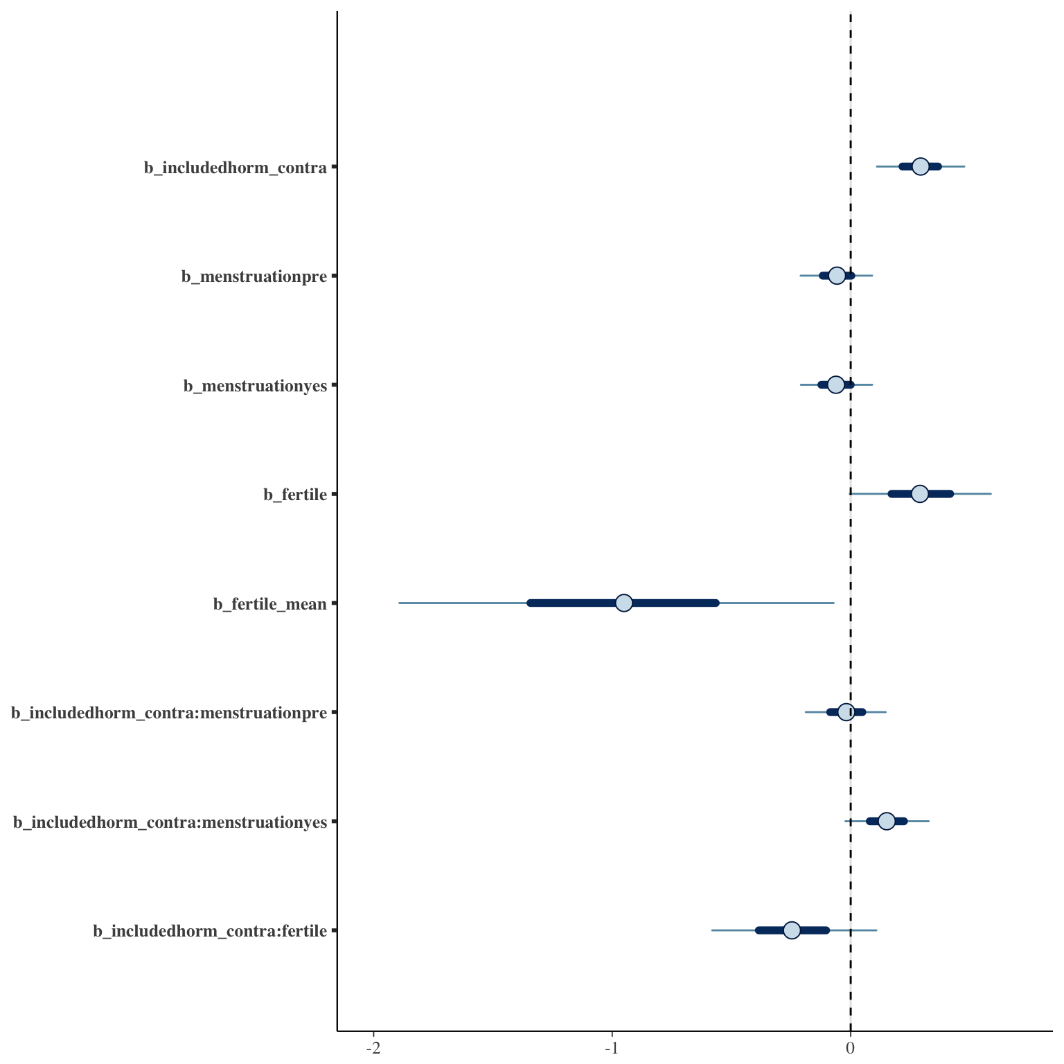
Estimate Est.Error l-95% CI u-95% CI Eff.Sample Rhat
Intercept[1] 1.43 0.13 1.17 1.67 1109 1.00
Intercept[2] 1.67 0.13 1.41 1.91 1111 1.00
Intercept[3] 1.89 0.13 1.63 2.13 979 1.00
Intercept[4] 2.40 0.13 2.15 2.65 988 1.00
Intercept[5] 2.93 0.13 2.67 3.17 1007 1.00
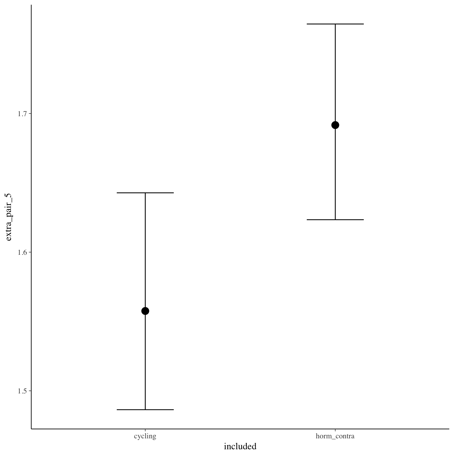
includedhorm_contra 0.29 0.11 0.08 0.51 769 1.01
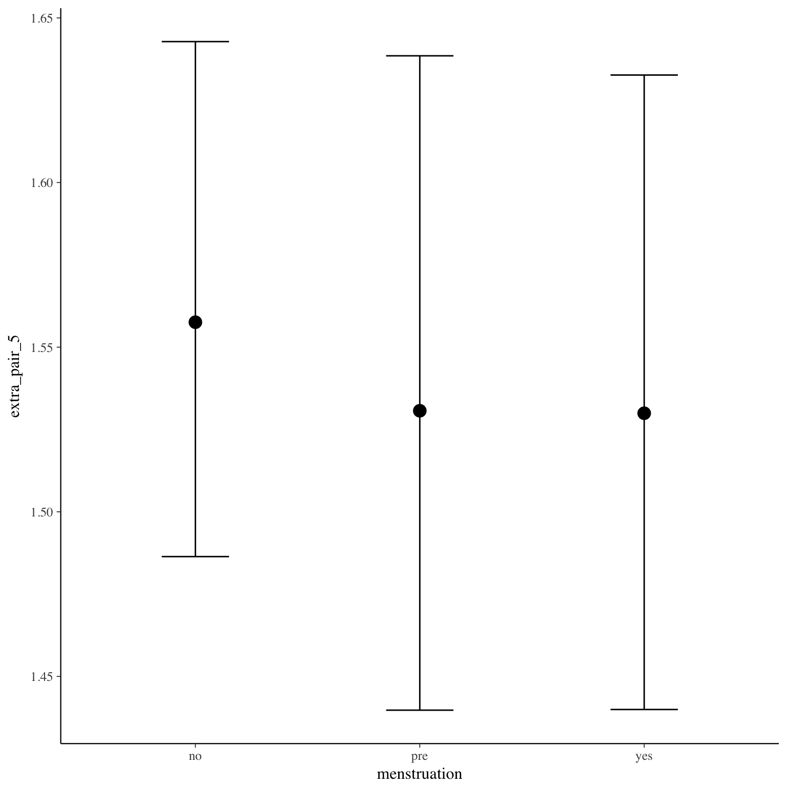
menstruationpre -0.06 0.09 -0.24 0.12 1695 1.00
menstruationyes -0.06 0.09 -0.23 0.12 1889 1.00
fertile 0.29 0.18 -0.07 0.65 1734 1.00
fertile_mean -0.96 0.56 -2.10 0.13 1510 1.00
includedhorm_contra:menstruationpre -0.02 0.10 -0.22 0.18 1933 1.00
includedhorm_contra:menstruationyes 0.15 0.11 -0.06 0.36 1859 1.00
includedhorm_contra:fertile -0.24 0.21 -0.66 0.18 1718 1.00
Samples were drawn using sampling(NUTS). For each parameter, Eff.Sample
is a crude measure of effective sample size, and Rhat is the potential
scale reduction factor on split chains (at convergence, Rhat = 1).
Coefficient plot
Marginal effect plots
Diagnostics
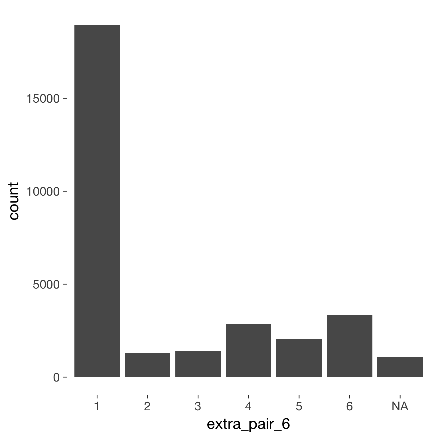
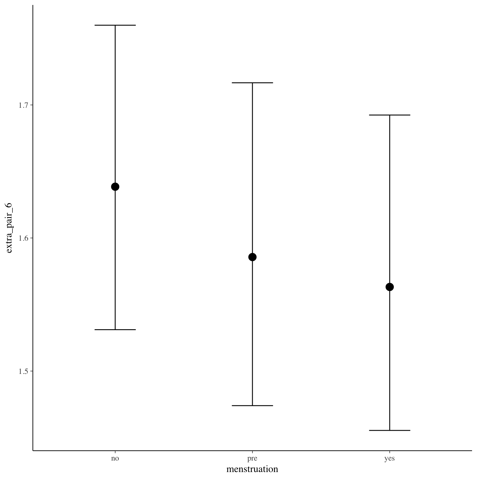
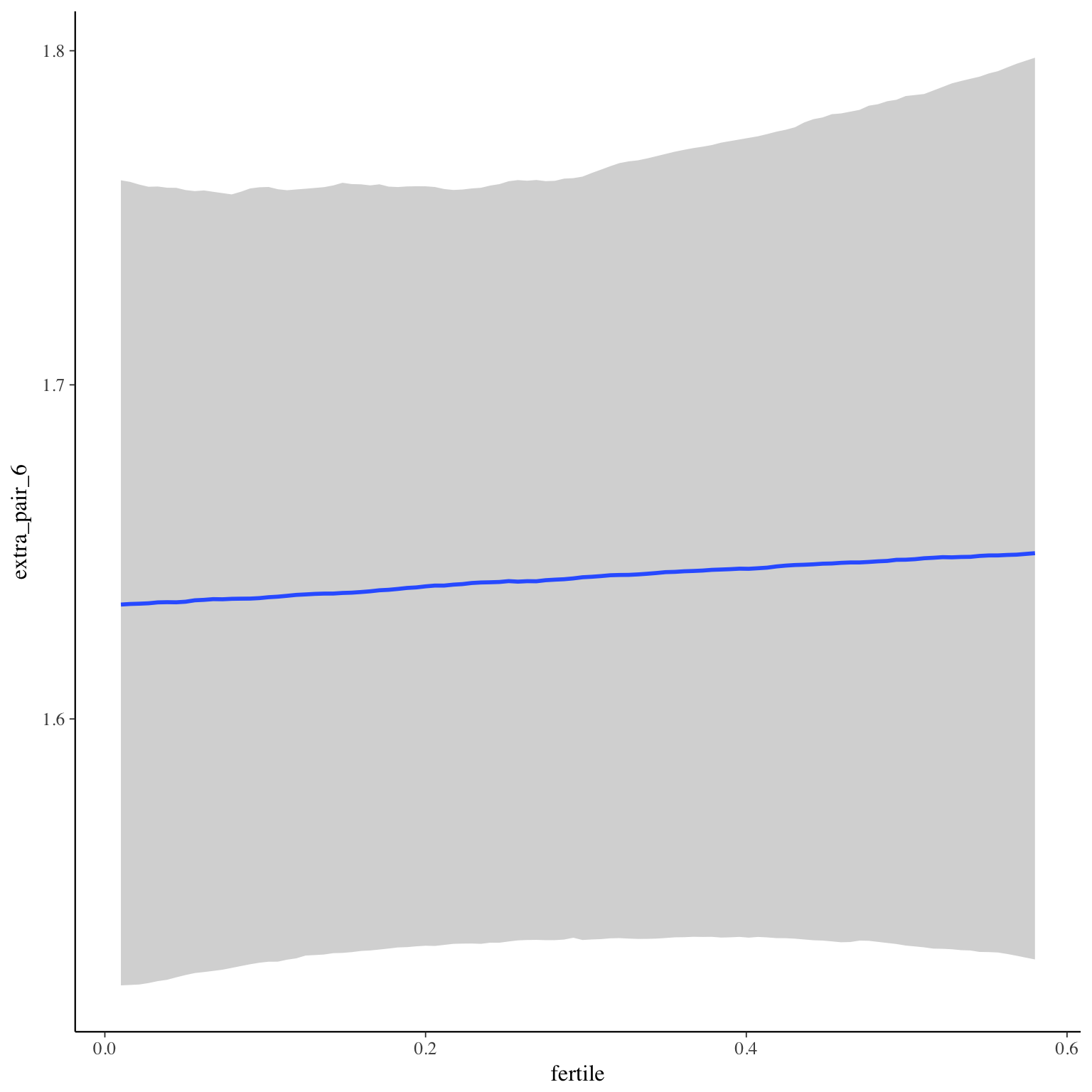
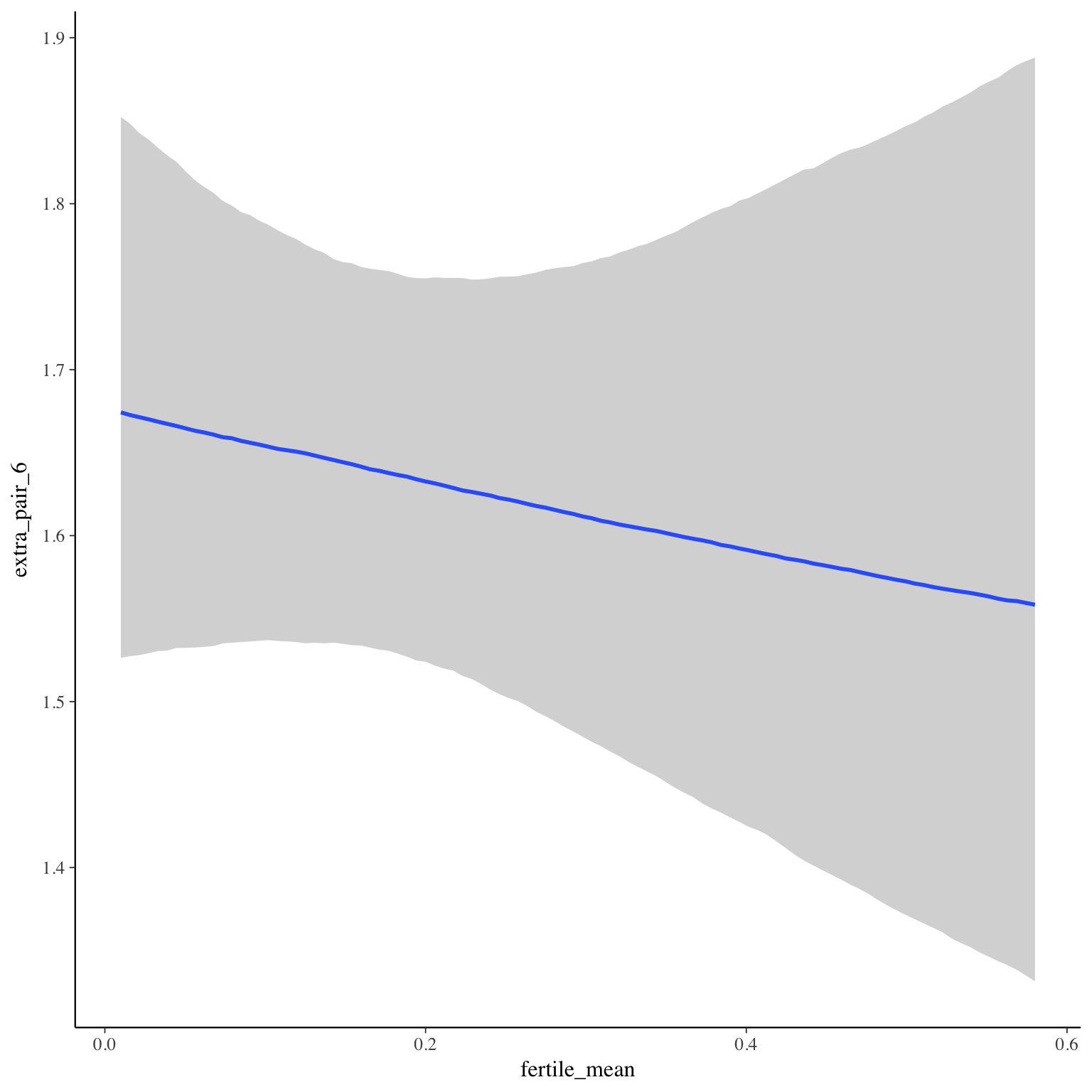
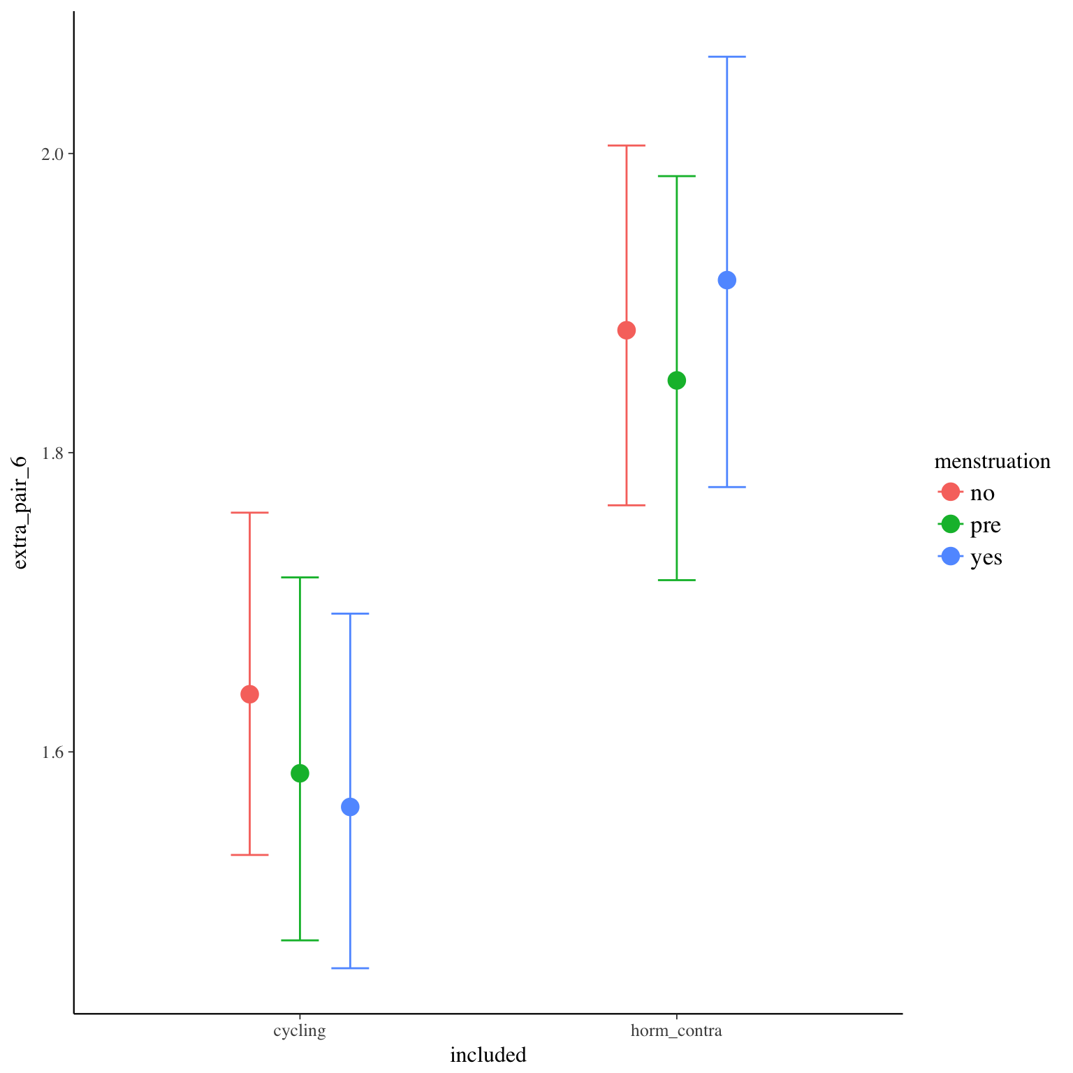
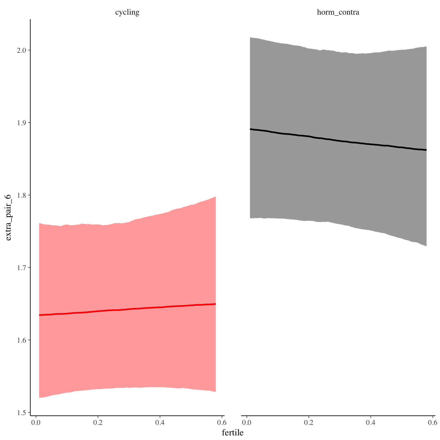
extra_pair_6
Item text:
… bin ich ohne meinen Partner an einen Ort gegangen, wo man Männer treffen kann.
Item translation:
52. I went out without my partner to a social event where one might meet men.
Choices:
| choice | value | frequency | percent |
|---|---|---|---|
| 1 | Stimme nicht zu | 18929 | 0.63 |
| 2 | Stimme überwiegend nicht zu | 1310 | 0.04 |
| 3 | Stimme eher nicht zu | 1403 | 0.05 |
| 4 | Stimme eher zu | 2853 | 0.1 |
| 5 | Stimme überwiegend zu | 2036 | 0.07 |
| 6 | Stimme voll zu | 3342 | 0.11 |
Model
Model summary
Family: cumulative(logit)
Formula: extra_pair_6 ~ included * (menstruation + fertile) + fertile_mean + (1 + fertile + menstruation | person)
disc = 1
Data: diary (Number of observations: 26544)
Samples: 4 chains, each with iter = 2000; warmup = 1000; thin = 1;
total post-warmup samples = 4000
ICs: LOO = 54212.02; WAIC = Not computed
Group-Level Effects:
~person (Number of levels: 1043)
Estimate Est.Error l-95% CI u-95% CI Eff.Sample Rhat
sd(Intercept) 1.97 0.07 1.84 2.11 909 1.00
sd(fertile) 1.58 0.15 1.28 1.87 440 1.01
sd(menstruationpre) 0.46 0.11 0.18 0.65 189 1.03
sd(menstruationyes) 0.62 0.09 0.43 0.77 358 1.01
cor(Intercept,fertile) -0.04 0.10 -0.24 0.15 1820 1.00
cor(Intercept,menstruationpre) -0.05 0.17 -0.37 0.32 1154 1.00
cor(fertile,menstruationpre) 0.28 0.19 -0.13 0.59 307 1.01
cor(Intercept,menstruationyes) -0.06 0.12 -0.28 0.19 1949 1.00
cor(fertile,menstruationyes) 0.23 0.14 -0.08 0.48 353 1.01
cor(menstruationpre,menstruationyes) 0.62 0.17 0.20 0.90 172 1.01
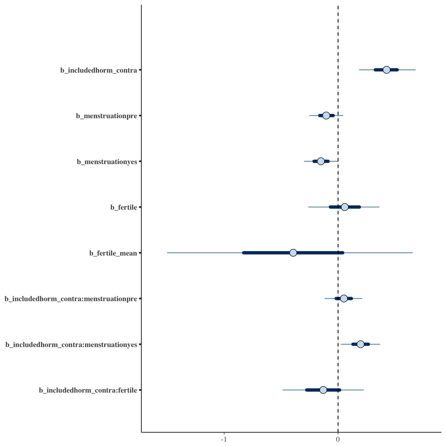
Population-Level Effects:
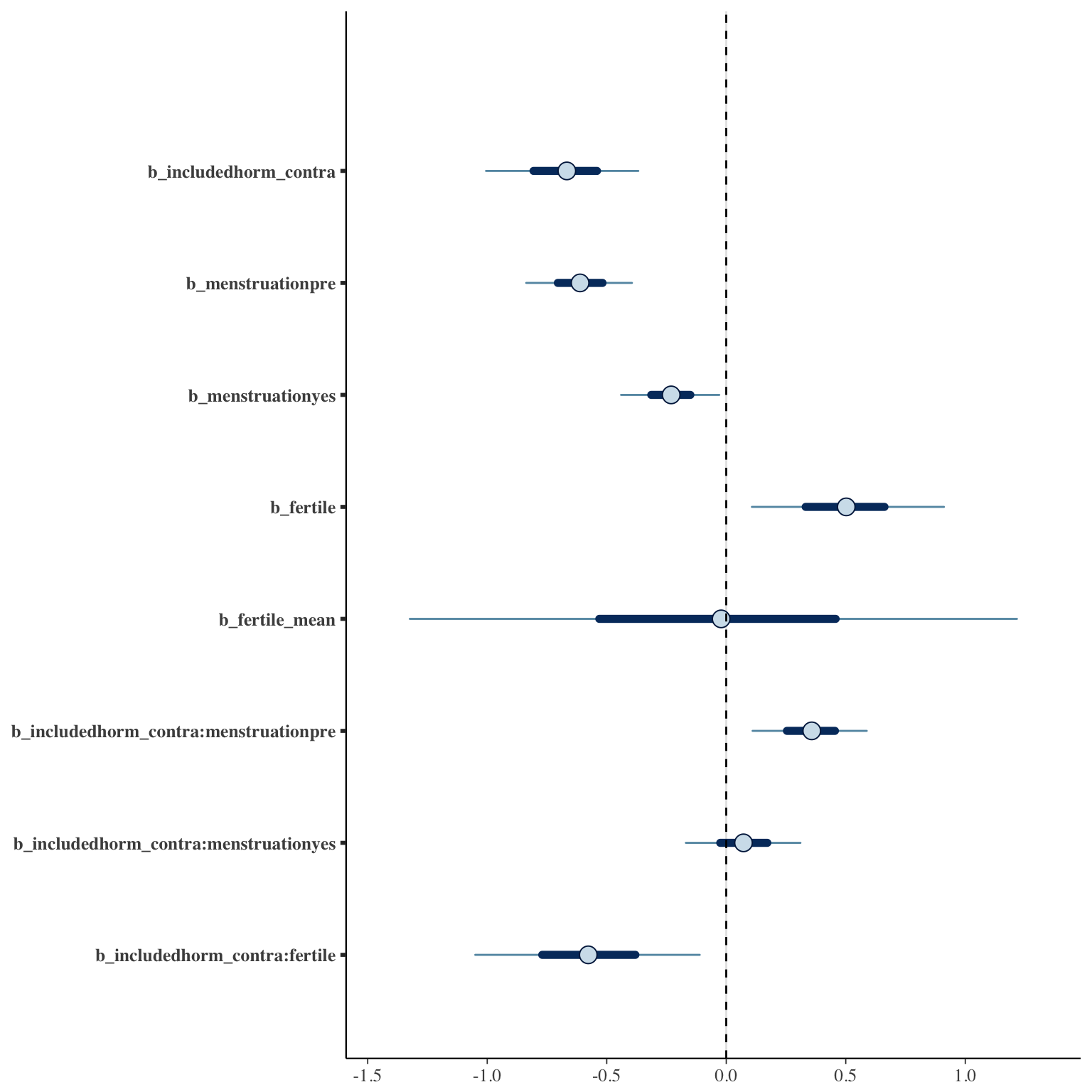
Estimate Est.Error l-95% CI u-95% CI Eff.Sample Rhat
Intercept[1] 1.16 0.16 0.85 1.47 543 1.01
Intercept[2] 1.46 0.16 1.15 1.78 547 1.01
Intercept[3] 1.81 0.16 1.50 2.12 548 1.01
Intercept[4] 2.60 0.16 2.29 2.92 552 1.01
Intercept[5] 3.36 0.16 3.05 3.68 557 1.01
includedhorm_contra 0.43 0.15 0.14 0.73 399 1.01
menstruationpre -0.10 0.09 -0.27 0.07 2003 1.00
menstruationyes -0.15 0.09 -0.32 0.02 1925 1.00
fertile 0.06 0.19 -0.32 0.43 1915 1.00
fertile_mean -0.41 0.66 -1.74 0.88 1153 1.00
includedhorm_contra:menstruationpre 0.05 0.10 -0.15 0.24 2191 1.00
includedhorm_contra:menstruationyes 0.20 0.10 0.00 0.40 2039 1.00
includedhorm_contra:fertile -0.13 0.22 -0.55 0.29 1885 1.00
Samples were drawn using sampling(NUTS). For each parameter, Eff.Sample
is a crude measure of effective sample size, and Rhat is the potential
scale reduction factor on split chains (at convergence, Rhat = 1).
Coefficient plot
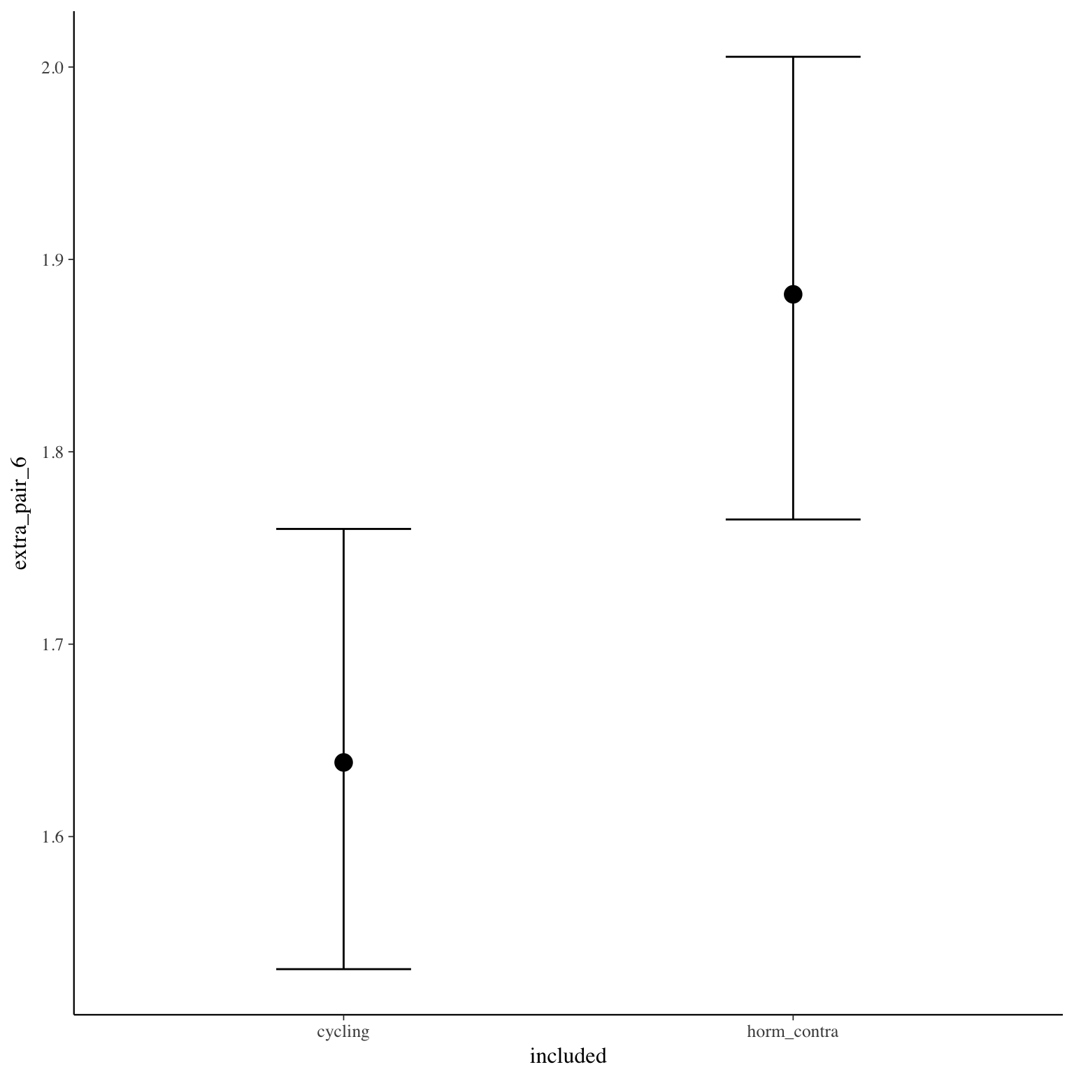
Marginal effect plots
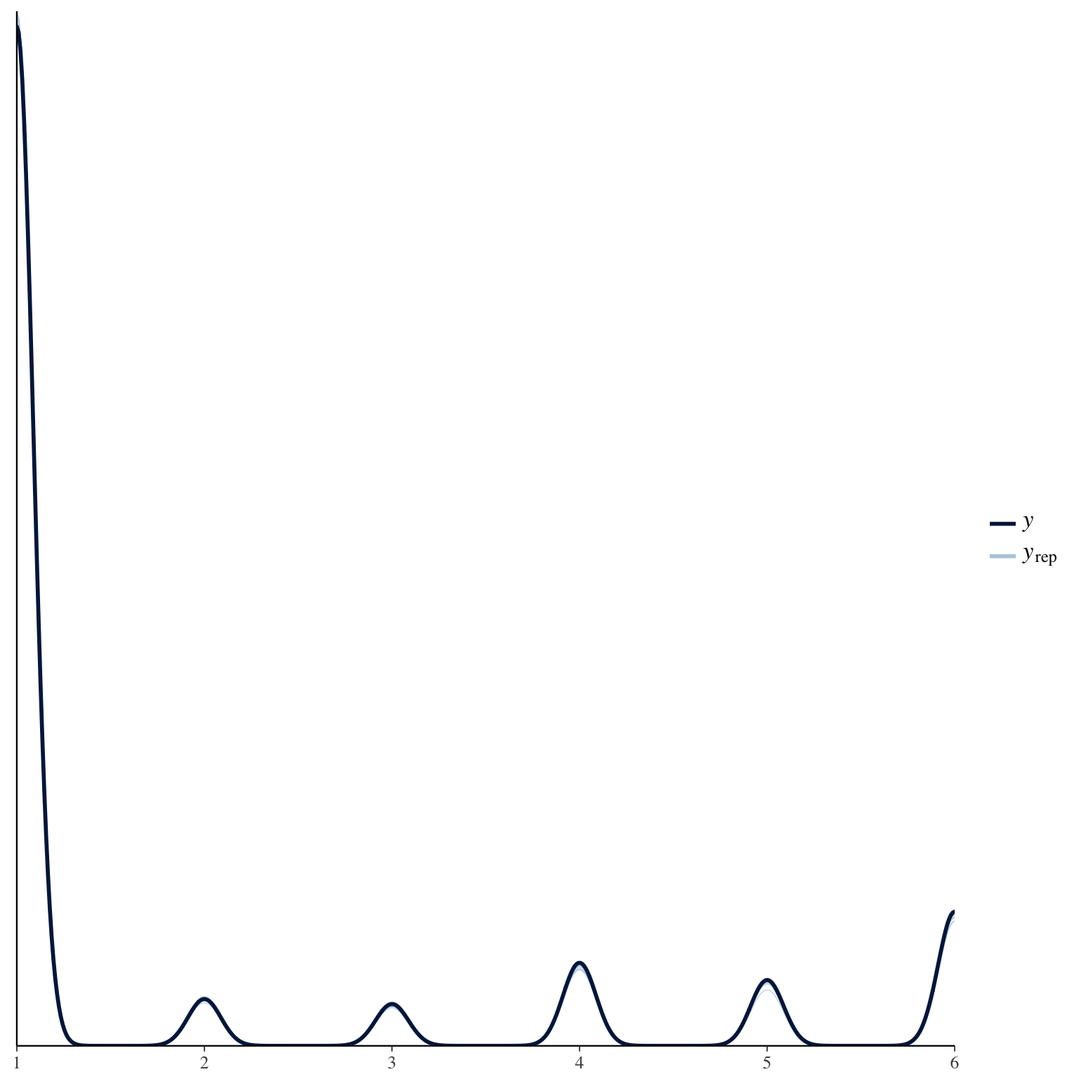
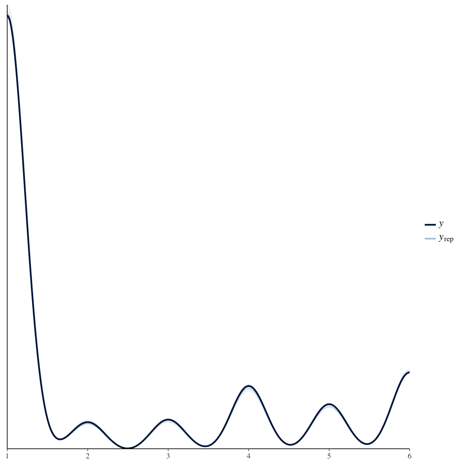
Diagnostics
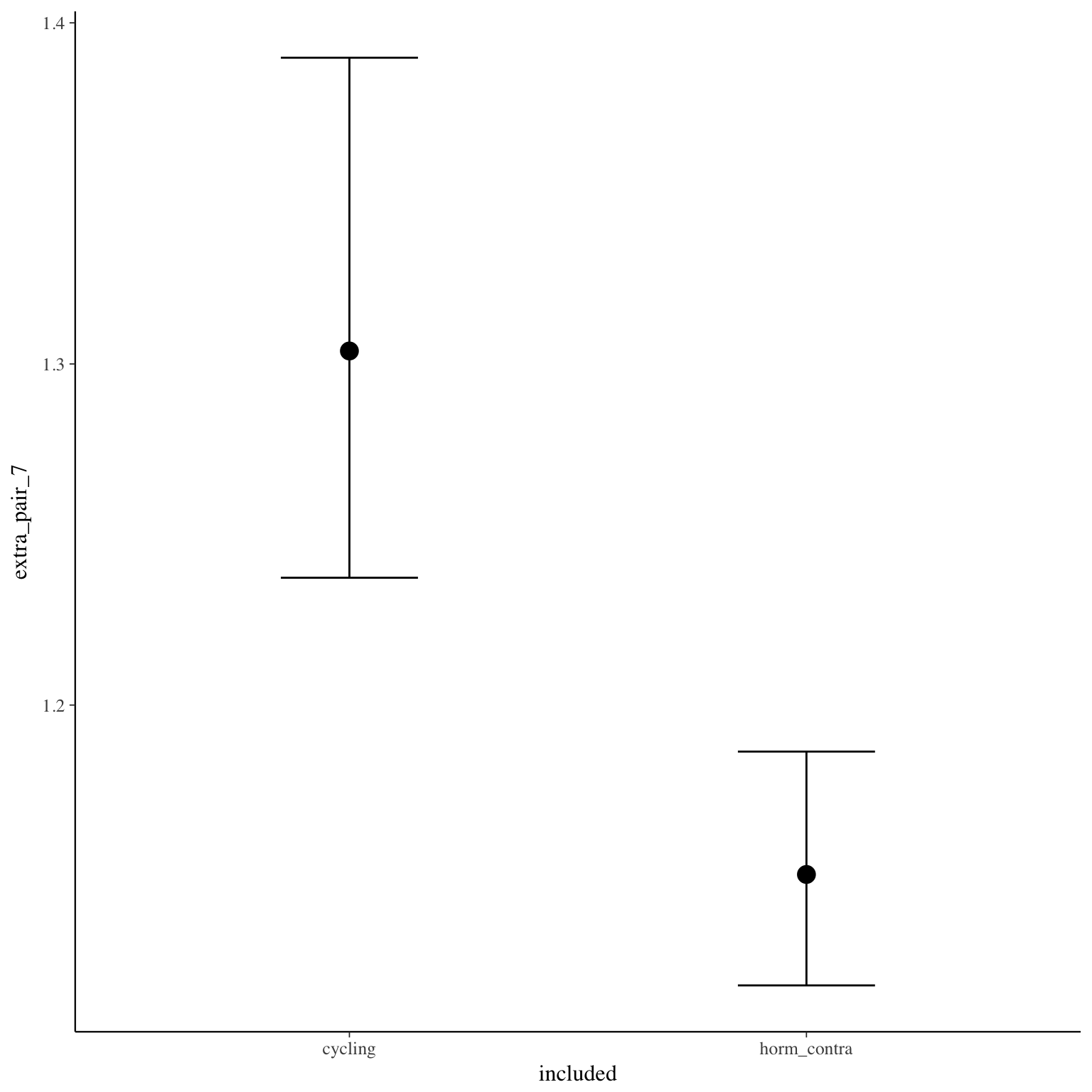
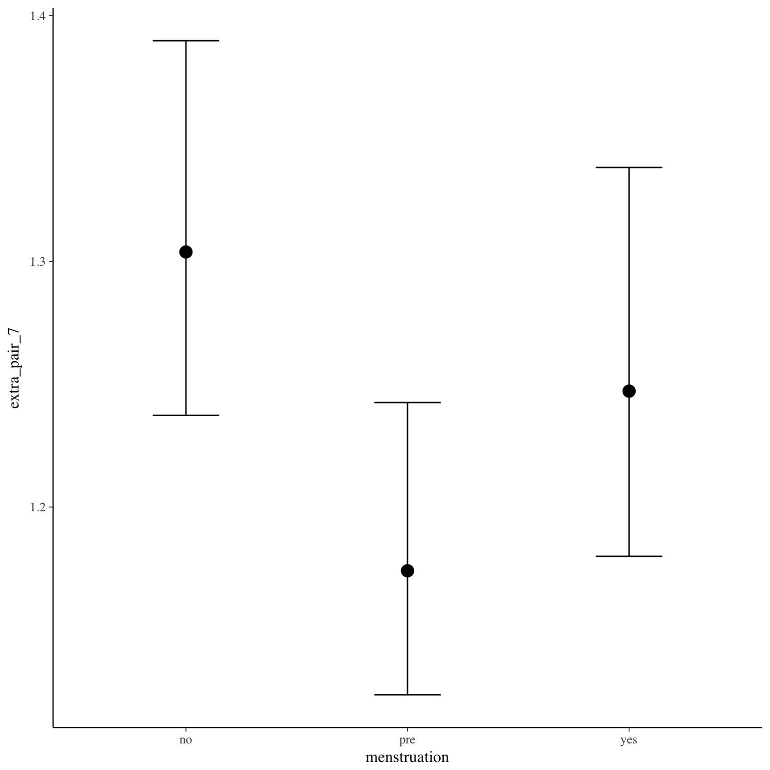
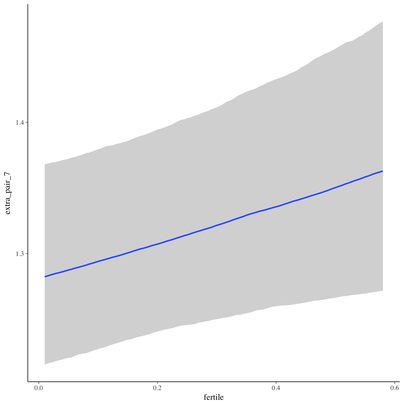
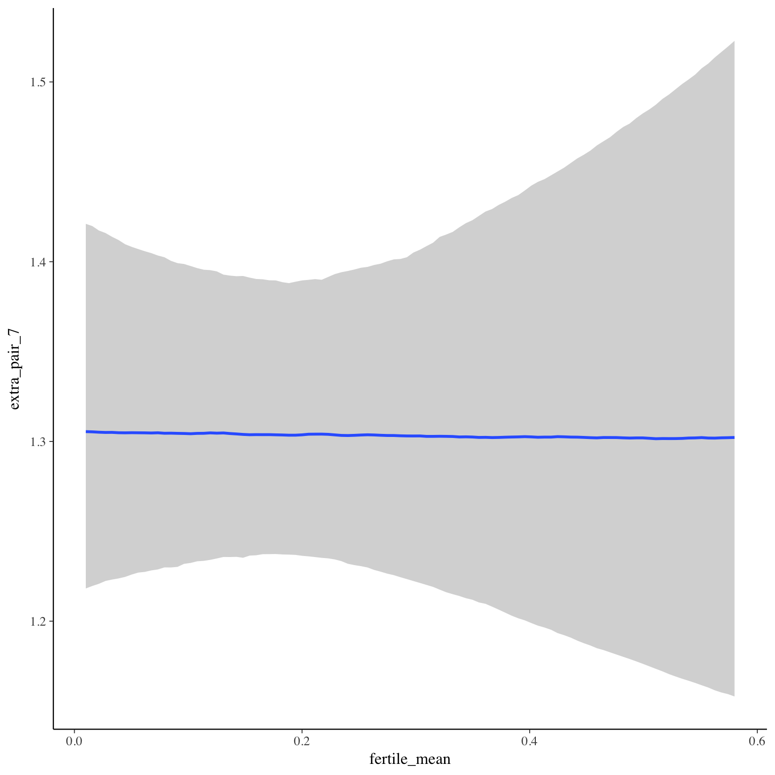
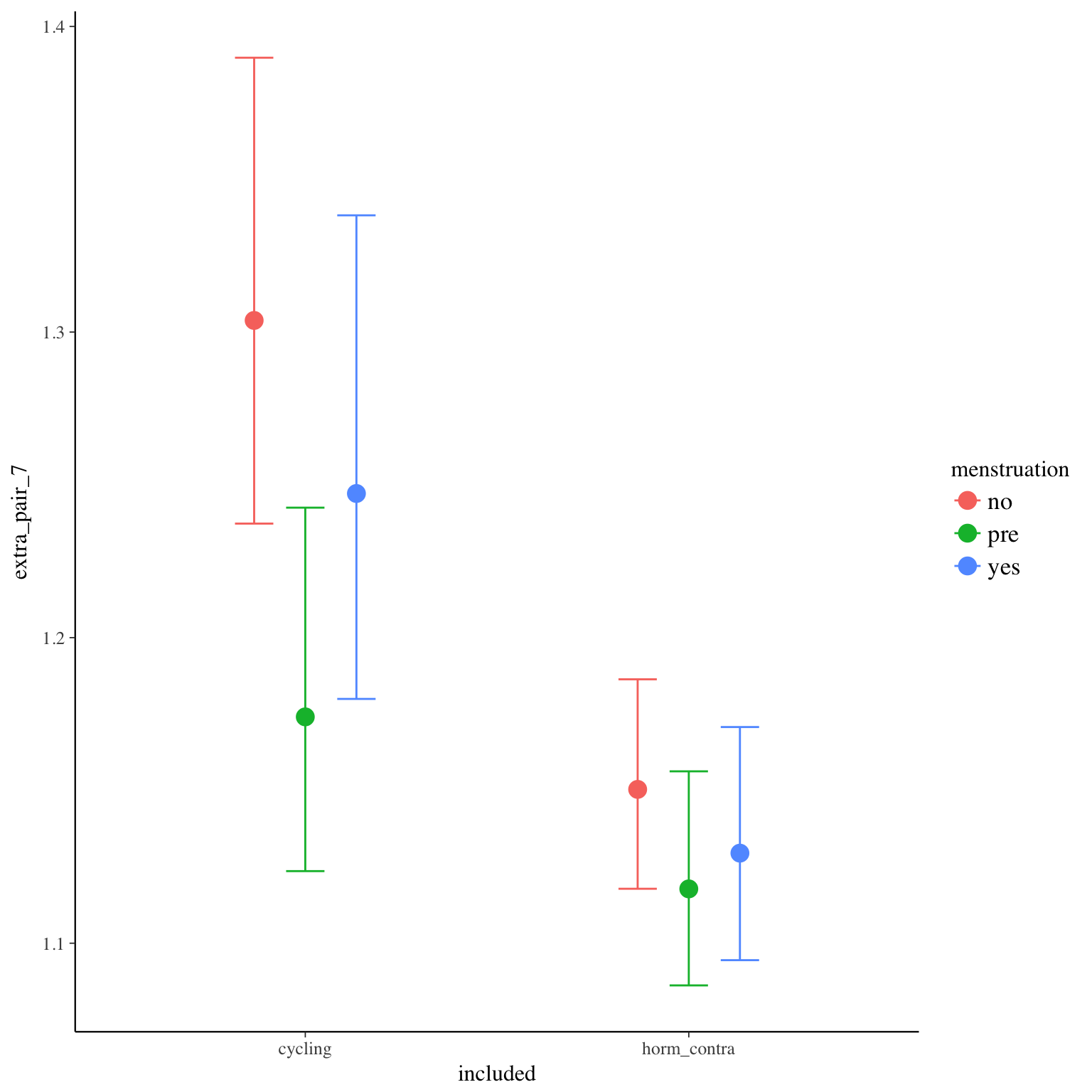
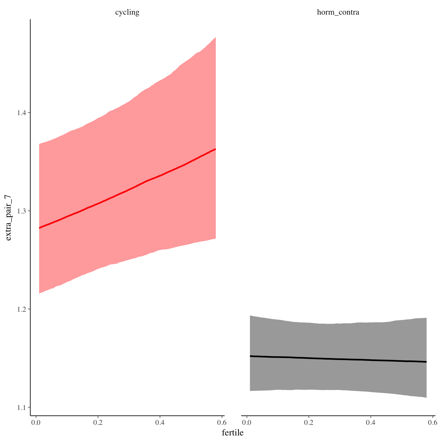
extra_pair_7
Item text:
… habe ich mir Gedanken über einen anderen potentiellen Partner gemacht.
Item translation:
53. I thought about another potential partner.
Choices:
| choice | value | frequency | percent |
|---|---|---|---|
| 1 | Stimme nicht zu | 22819 | 0.76 |
| 2 | Stimme überwiegend nicht zu | 2032 | 0.07 |
| 3 | Stimme eher nicht zu | 1579 | 0.05 |
| 4 | Stimme eher zu | 1865 | 0.06 |
| 5 | Stimme überwiegend zu | 875 | 0.03 |
| 6 | Stimme voll zu | 703 | 0.02 |

Model
Model summary
 Family: cumulative(logit)
Formula: extra_pair_7 ~ included * (menstruation + fertile) + fertile_mean + (1 + fertile + menstruation | person)
         disc = 1
   Data: diary (Number of observations: 26544)
Samples: 4 chains, each with iter = 2000; warmup = 1000; thin = 1;
         total post-warmup samples = 4000
    ICs: LOO = 34839.06; WAIC = Not computed

Group-Level Effects:
~person (Number of levels: 1043)
                                     Estimate Est.Error l-95% CI u-95% CI Eff.Sample Rhat
sd(Intercept)                            2.70      0.10     2.52     2.91        629 1.00
sd(fertile)                              2.41      0.19     2.05     2.79        625 1.01
sd(menstruationpre)                      1.03      0.10     0.84     1.23       1095 1.00
sd(menstruationyes)                      1.08      0.09     0.89     1.26        784 1.00
cor(Intercept,fertile)                  -0.21      0.08    -0.37    -0.04       1684 1.00
cor(Intercept,menstruationpre)           0.05      0.10    -0.16     0.25       1512 1.00
cor(fertile,menstruationpre)             0.24      0.10     0.02     0.44        756 1.00
cor(Intercept,menstruationyes)          -0.03      0.10    -0.21     0.16       1632 1.00
cor(fertile,menstruationyes)             0.53      0.09     0.35     0.69        749 1.01
cor(menstruationpre,menstruationyes)     0.60      0.09     0.41     0.75        774 1.00

Population-Level Effects:
                                    Estimate Est.Error l-95% CI u-95% CI Eff.Sample Rhat
Intercept[1]                            1.70      0.20     1.29     2.09        549    1
Intercept[2]                            2.46      0.20     2.07     2.86        556    1
Intercept[3]                            3.24      0.20     2.85     3.65        552    1
Intercept[4]                            4.66      0.21     4.26     5.06        516    1
Intercept[5]                            5.95      0.21     5.54     6.36        539    1
includedhorm_contra                    -0.67      0.19    -1.06    -0.31        493    1
menstruationpre                        -0.61      0.14    -0.88    -0.35       1838    1
menstruationyes                        -0.23      0.12    -0.48     0.01       1480    1
fertile                                 0.50      0.24     0.03     0.98       1304    1
fertile_mean                           -0.04      0.77    -1.65     1.43       1460    1
includedhorm_contra:menstruationpre     0.35      0.15     0.06     0.63       1868    1
includedhorm_contra:menstruationyes     0.07      0.14    -0.21     0.36       1954    1
includedhorm_contra:fertile            -0.58      0.28    -1.14    -0.01       1257    1

Samples were drawn using sampling(NUTS). For each parameter, Eff.Sample
is a crude measure of effective sample size, and Rhat is the potential
scale reduction factor on split chains (at convergence, Rhat = 1).
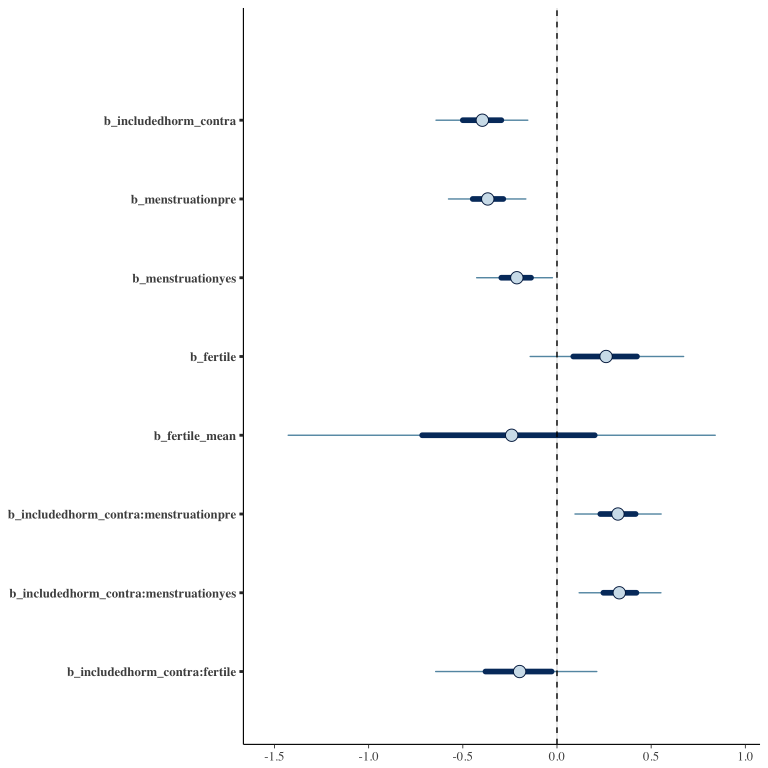
Coefficient plot
Marginal effect plots
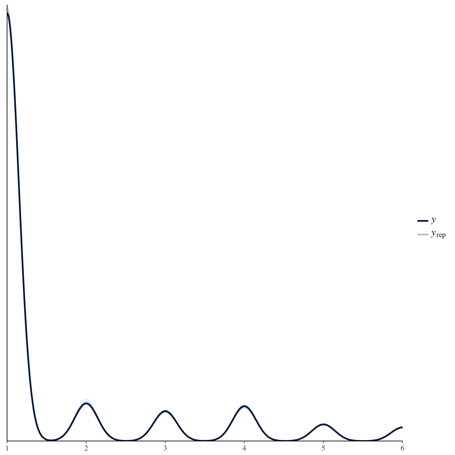
Diagnostics
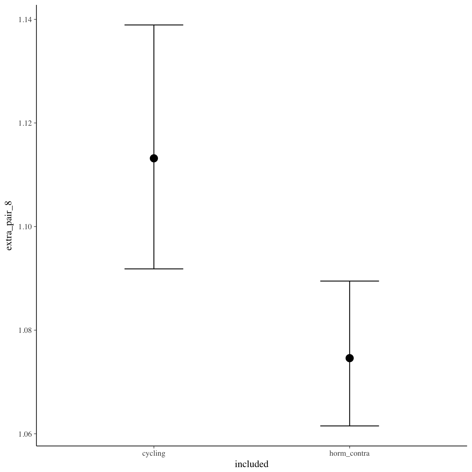
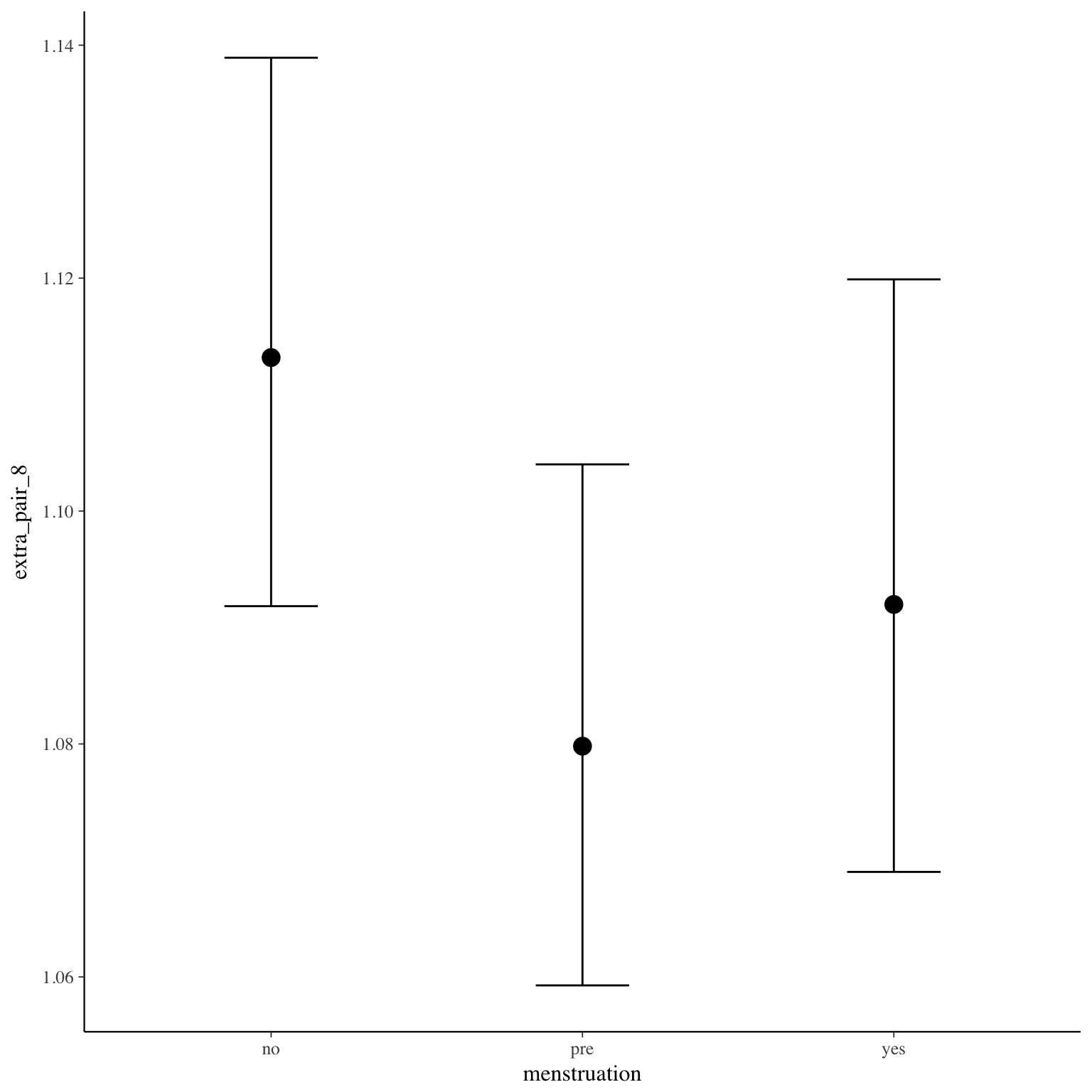
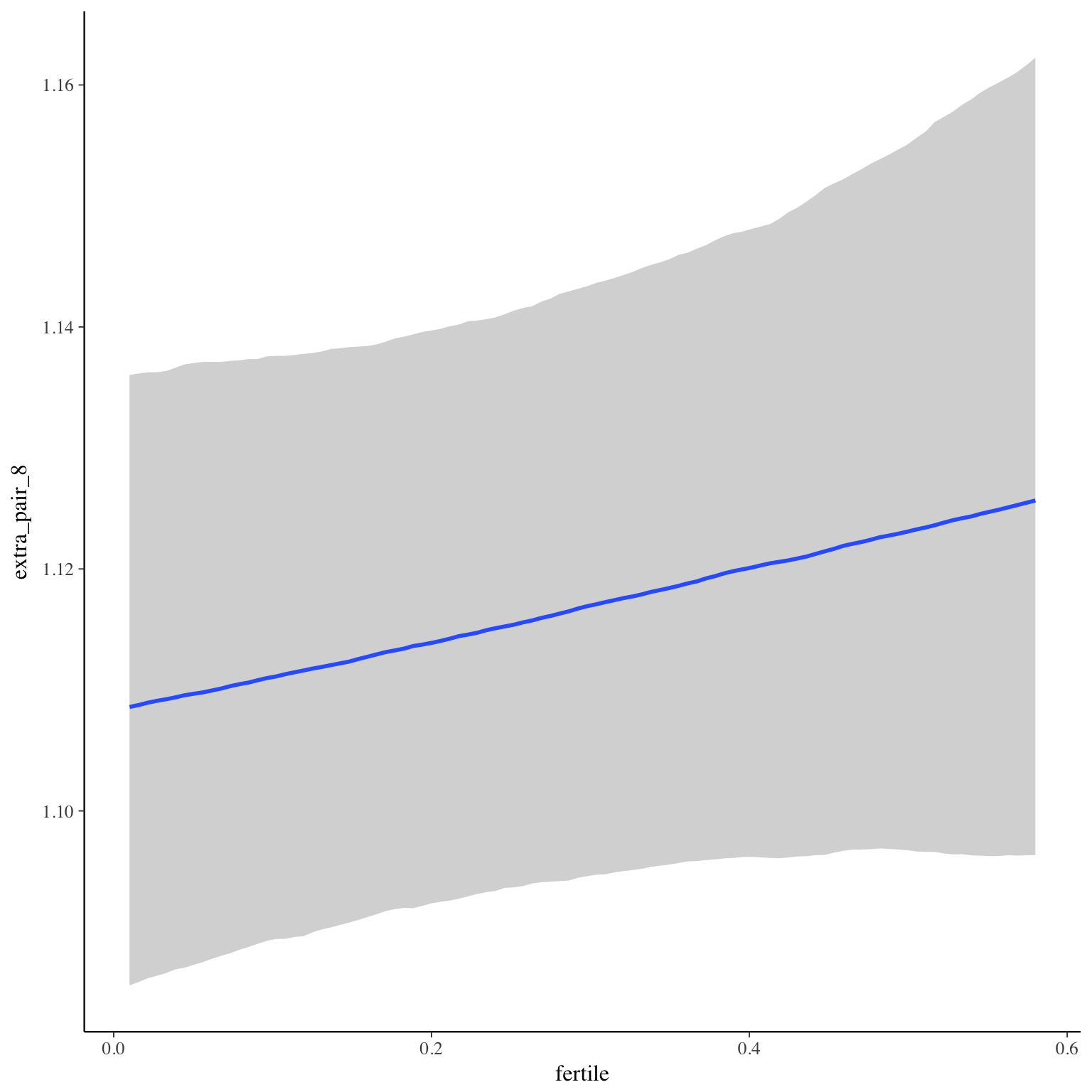
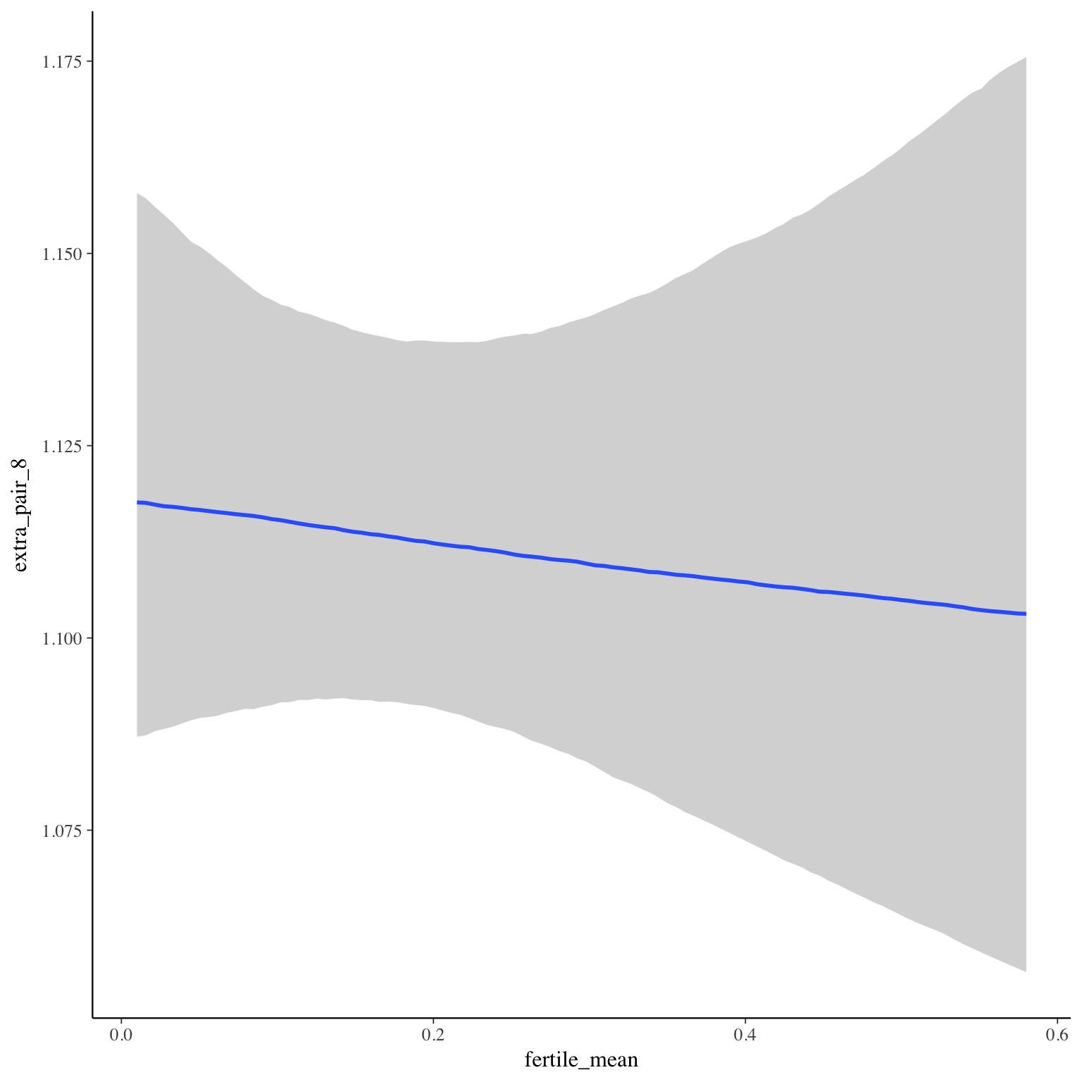
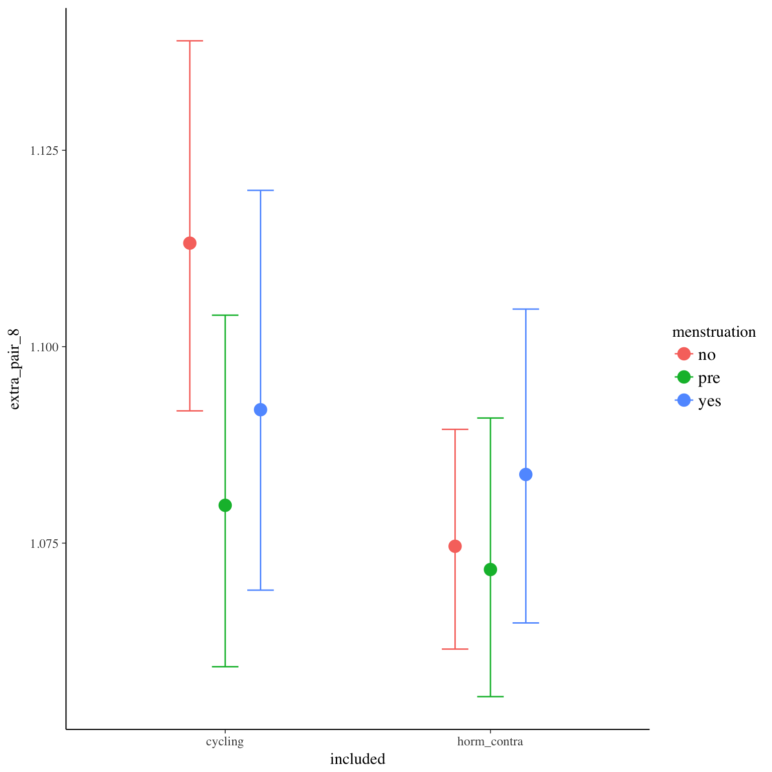
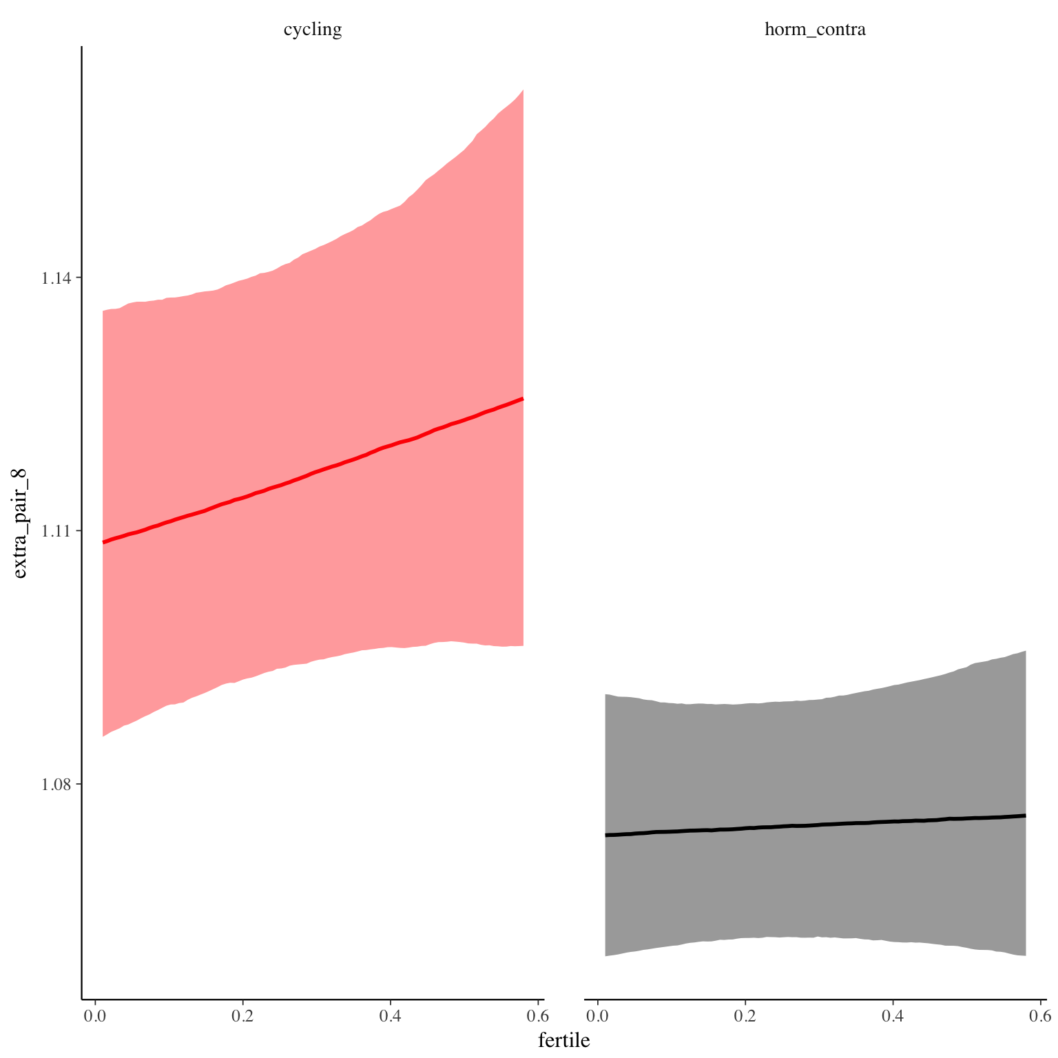
extra_pair_8
Item text:
… habe ich mit Männern geflirtet, die ich nicht kannte.
Item translation:
50. I flirted with strangers.
Choices:
| choice | value | frequency | percent |
|---|---|---|---|
| 1 | Stimme nicht zu | 26492 | 0.89 |
| 2 | Stimme überwiegend nicht zu | 1258 | 0.04 |
| 3 | Stimme eher nicht zu | 880 | 0.03 |
| 4 | Stimme eher zu | 766 | 0.03 |
| 5 | Stimme überwiegend zu | 277 | 0.01 |
| 6 | Stimme voll zu | 200 | 0.01 |

Model
Model summary
 Family: cumulative(logit)
Formula: extra_pair_8 ~ included * (menstruation + fertile) + fertile_mean + (1 + fertile + menstruation | person)
         disc = 1
   Data: diary (Number of observations: 26544)
Samples: 4 chains, each with iter = 2000; warmup = 1000; thin = 1;
         total post-warmup samples = 4000
    ICs: LOO = 22448.63; WAIC = Not computed

Group-Level Effects:
~person (Number of levels: 1043)
                                     Estimate Est.Error l-95% CI u-95% CI Eff.Sample Rhat
sd(Intercept)                            1.82      0.08     1.68     1.98        831 1.00
sd(fertile)                              0.69      0.32     0.07     1.28        157 1.01
sd(menstruationpre)                      0.19      0.14     0.01     0.50        337 1.01
sd(menstruationyes)                      0.28      0.17     0.01     0.62        341 1.01
cor(Intercept,fertile)                  -0.32      0.26    -0.77     0.29       1704 1.00
cor(Intercept,menstruationpre)          -0.02      0.37    -0.72     0.74       2803 1.00
cor(fertile,menstruationpre)             0.01      0.44    -0.81     0.81        831 1.00
cor(Intercept,menstruationyes)          -0.06      0.30    -0.65     0.58       2529 1.00
cor(fertile,menstruationyes)            -0.07      0.42    -0.84     0.70        591 1.01
cor(menstruationpre,menstruationyes)     0.25      0.44    -0.71     0.90        495 1.00

Population-Level Effects:
                                    Estimate Est.Error l-95% CI u-95% CI Eff.Sample Rhat
Intercept[1]                            2.75      0.17     2.43     3.09       1253    1
Intercept[2]                            3.46      0.17     3.13     3.80       1258    1
Intercept[3]                            4.15      0.17     3.82     4.49       1261    1
Intercept[4]                            5.23      0.18     4.90     5.58       1349    1
Intercept[5]                            6.20      0.19     5.83     6.57       1463    1
includedhorm_contra                    -0.40      0.15    -0.69    -0.10        842    1
menstruationpre                        -0.37      0.12    -0.62    -0.13       2019    1
menstruationyes                        -0.22      0.12    -0.47     0.01       2275    1
fertile                                 0.26      0.25    -0.22     0.75       2262    1
fertile_mean                           -0.26      0.69    -1.62     1.04       1597    1
includedhorm_contra:menstruationpre     0.32      0.14     0.05     0.60       2446    1
includedhorm_contra:menstruationyes     0.33      0.13     0.08     0.59       2924    1
includedhorm_contra:fertile            -0.21      0.26    -0.74     0.30       2198    1

Samples were drawn using sampling(NUTS). For each parameter, Eff.Sample
is a crude measure of effective sample size, and Rhat is the potential
scale reduction factor on split chains (at convergence, Rhat = 1).
Coefficient plot
Marginal effect plots
Diagnostics
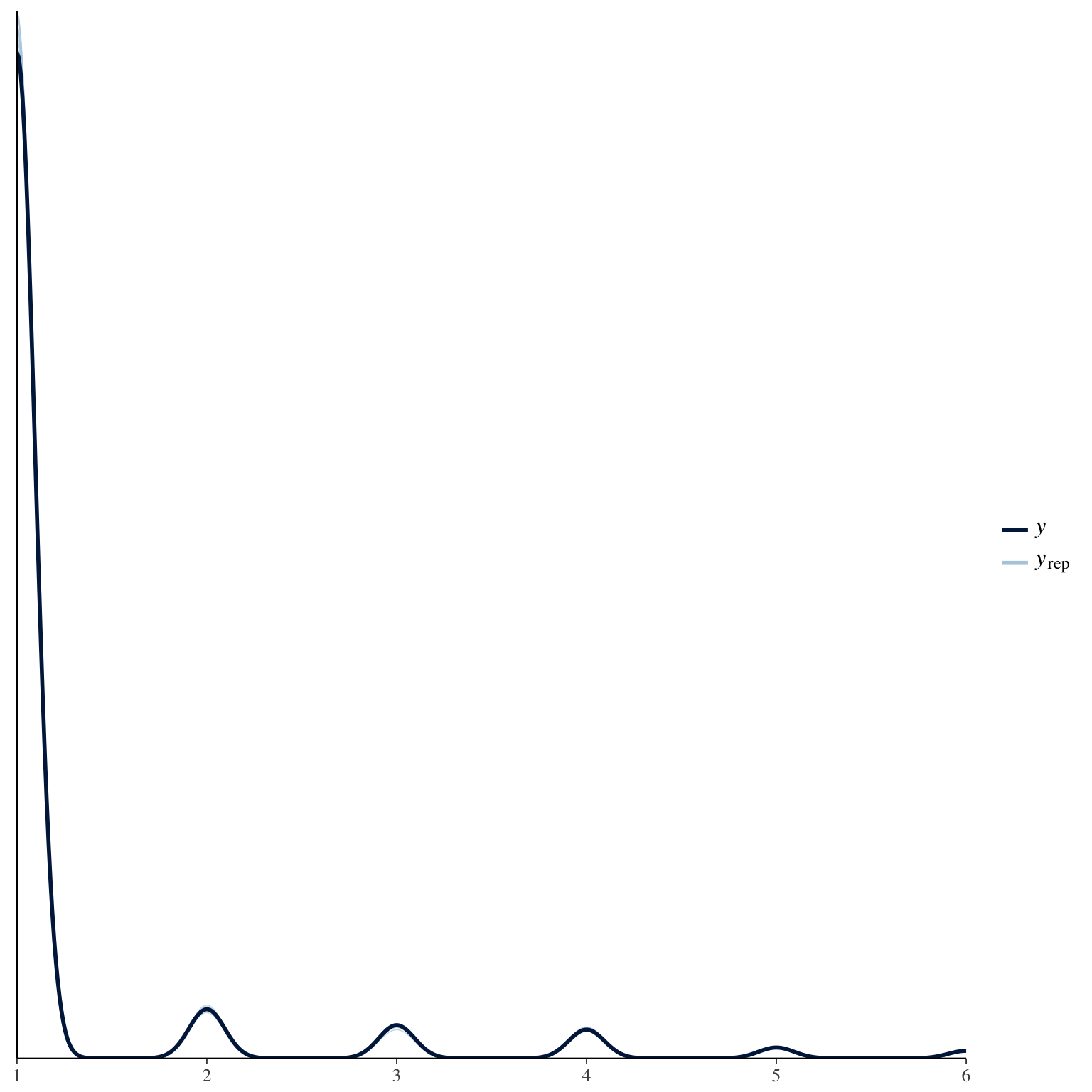
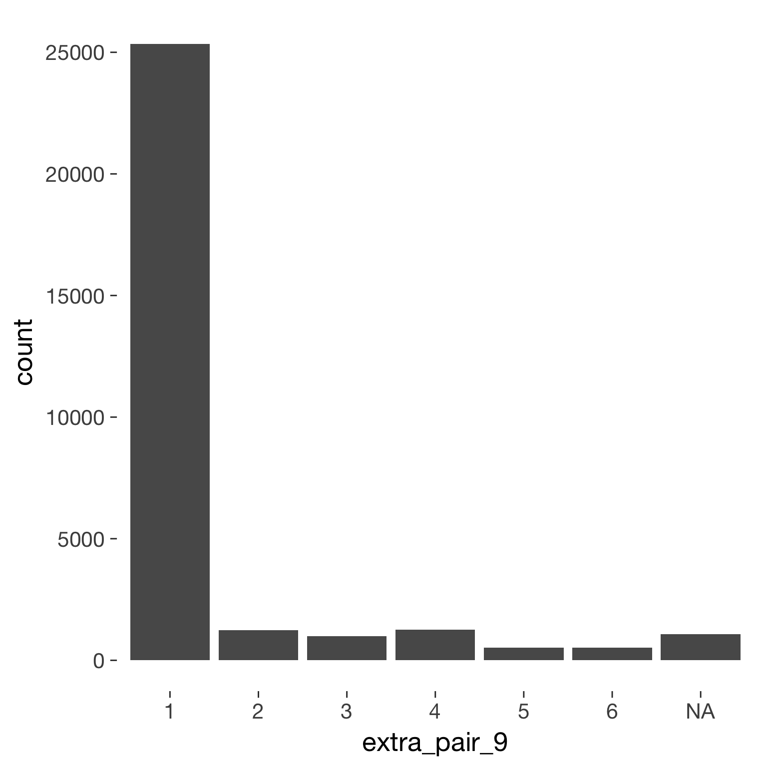
extra_pair_9
Item text:
… habe ich mit Freunden, Kollegen oder Bekannten geflirtet.
Item translation:
49. I flirted with friends, acquaintances, or colleagues.
Choices:
| choice | value | frequency | percent |
|---|---|---|---|
| 1 | Stimme nicht zu | 25338 | 0.85 |
| 2 | Stimme überwiegend nicht zu | 1245 | 0.04 |
| 3 | Stimme eher nicht zu | 995 | 0.03 |
| 4 | Stimme eher zu | 1262 | 0.04 |
| 5 | Stimme überwiegend zu | 522 | 0.02 |
| 6 | Stimme voll zu | 511 | 0.02 |
Model
Model summary
 Family: cumulative(logit)
Formula: extra_pair_9 ~ included * (menstruation + fertile) + fertile_mean + (1 + fertile + menstruation | person)
         disc = 1
   Data: diary (Number of observations: 26544)
Samples: 4 chains, each with iter = 2000; warmup = 1000; thin = 1;
         total post-warmup samples = 4000
    ICs: LOO = 28373.84; WAIC = Not computed

Group-Level Effects:
~person (Number of levels: 1043)
                                     Estimate Est.Error l-95% CI u-95% CI Eff.Sample Rhat
sd(Intercept)                            2.00      0.08     1.84     2.18        787 1.01
sd(fertile)                              1.41      0.21     1.00     1.82        422 1.01
sd(menstruationpre)                      0.53      0.14     0.25     0.79        330 1.01
sd(menstruationyes)                      0.62      0.14     0.30     0.88        272 1.02
cor(Intercept,fertile)                  -0.17      0.13    -0.41     0.09       2484 1.00
cor(Intercept,menstruationpre)           0.11      0.19    -0.26     0.47       1265 1.00
cor(fertile,menstruationpre)            -0.35      0.28    -0.86     0.17        295 1.02
cor(Intercept,menstruationyes)           0.06      0.17    -0.26     0.40        767 1.01
cor(fertile,menstruationyes)             0.33      0.22    -0.15     0.70        353 1.01
cor(menstruationpre,menstruationyes)     0.27      0.28    -0.36     0.72        269 1.01

Population-Level Effects:
                                    Estimate Est.Error l-95% CI u-95% CI Eff.Sample Rhat
Intercept[1]                            2.39      0.18     2.05     2.73        825    1
Intercept[2]                            2.93      0.18     2.58     3.27        827    1
Intercept[3]                            3.47      0.18     3.13     3.82        812    1
Intercept[4]                            4.53      0.18     4.19     4.88        850    1
Intercept[5]                            5.45      0.18     5.09     5.81        861    1
includedhorm_contra                    -0.51      0.16    -0.82    -0.20        506    1
menstruationpre                        -0.40      0.13    -0.65    -0.15       2240    1
menstruationyes                        -0.21      0.12    -0.44     0.02       2380    1
fertile                                 0.34      0.23    -0.11     0.78       2133    1
fertile_mean                            0.31      0.71    -1.02     1.72       1529    1
includedhorm_contra:menstruationpre     0.27      0.13     0.01     0.53       2933    1
includedhorm_contra:menstruationyes     0.01      0.13    -0.25     0.26       3015    1
includedhorm_contra:fertile            -0.45      0.26    -0.98     0.06       2528    1

Samples were drawn using sampling(NUTS). For each parameter, Eff.Sample
is a crude measure of effective sample size, and Rhat is the potential
scale reduction factor on split chains (at convergence, Rhat = 1).
Coefficient plot
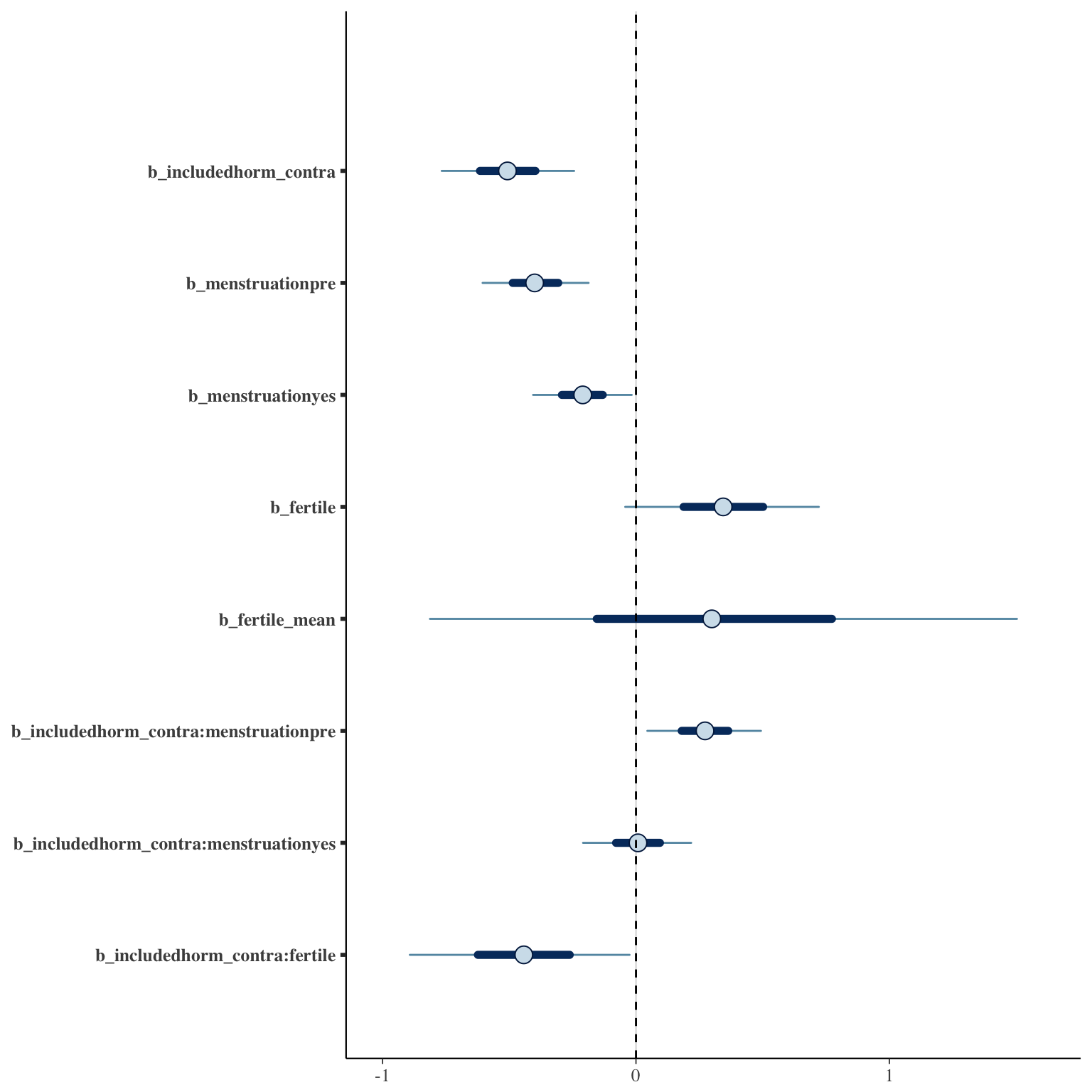
Marginal effect plots

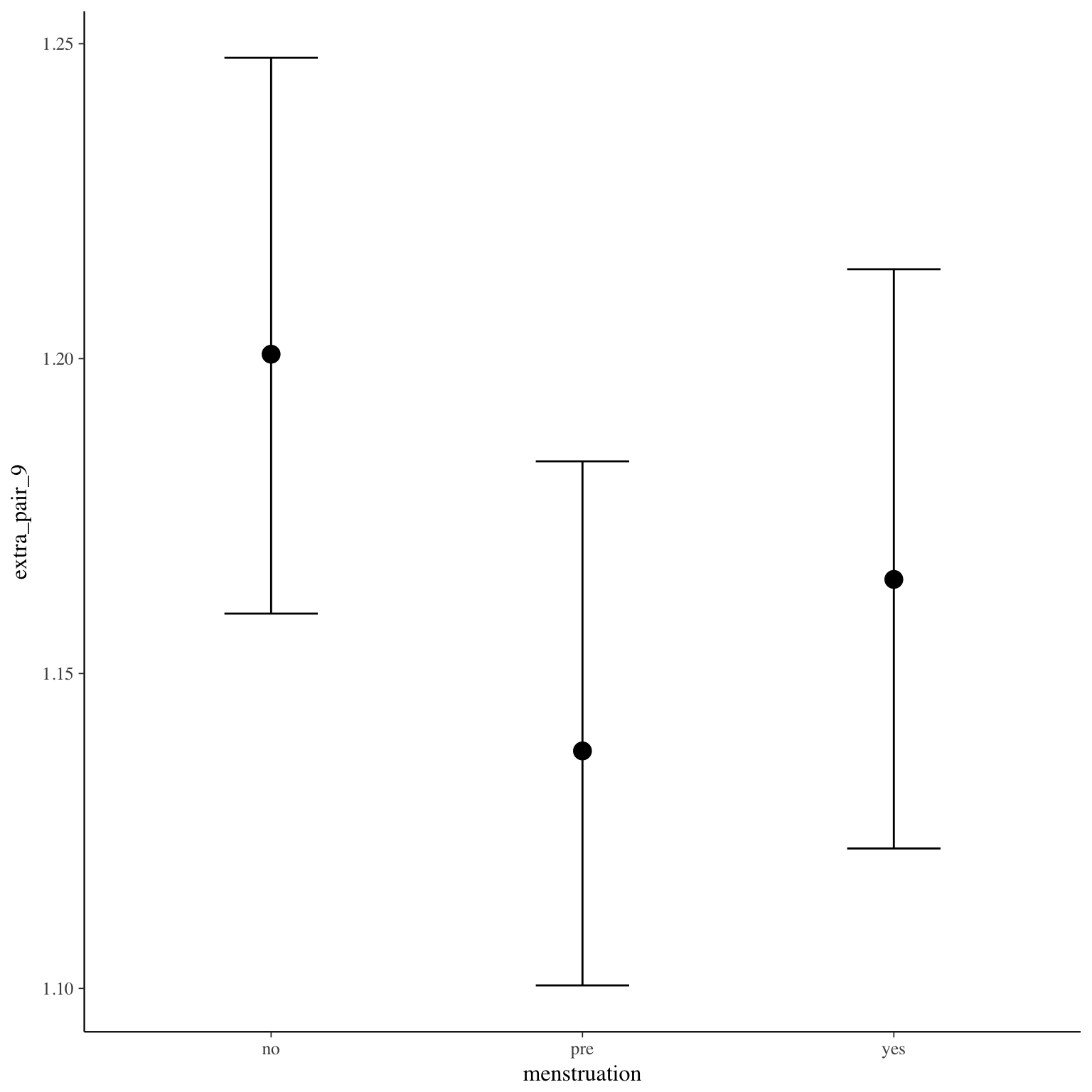
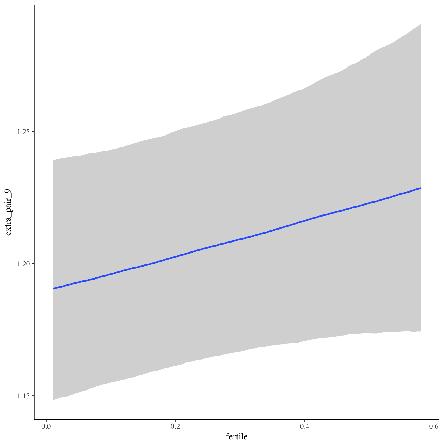
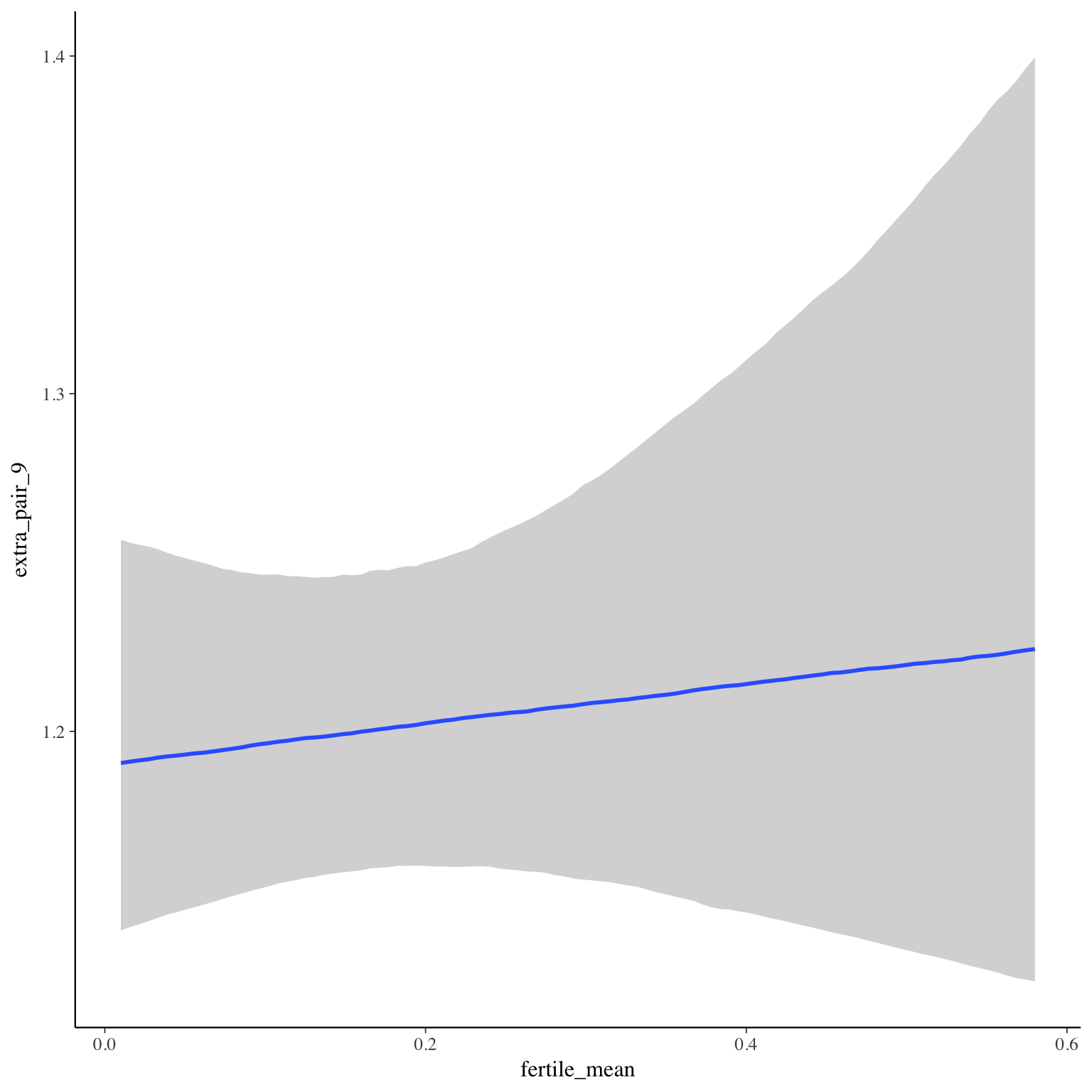
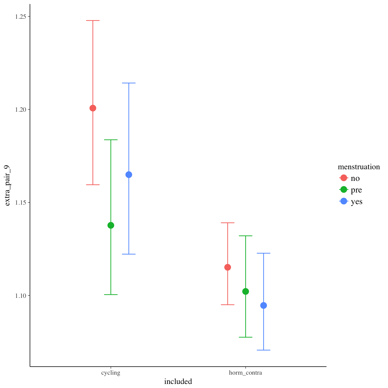
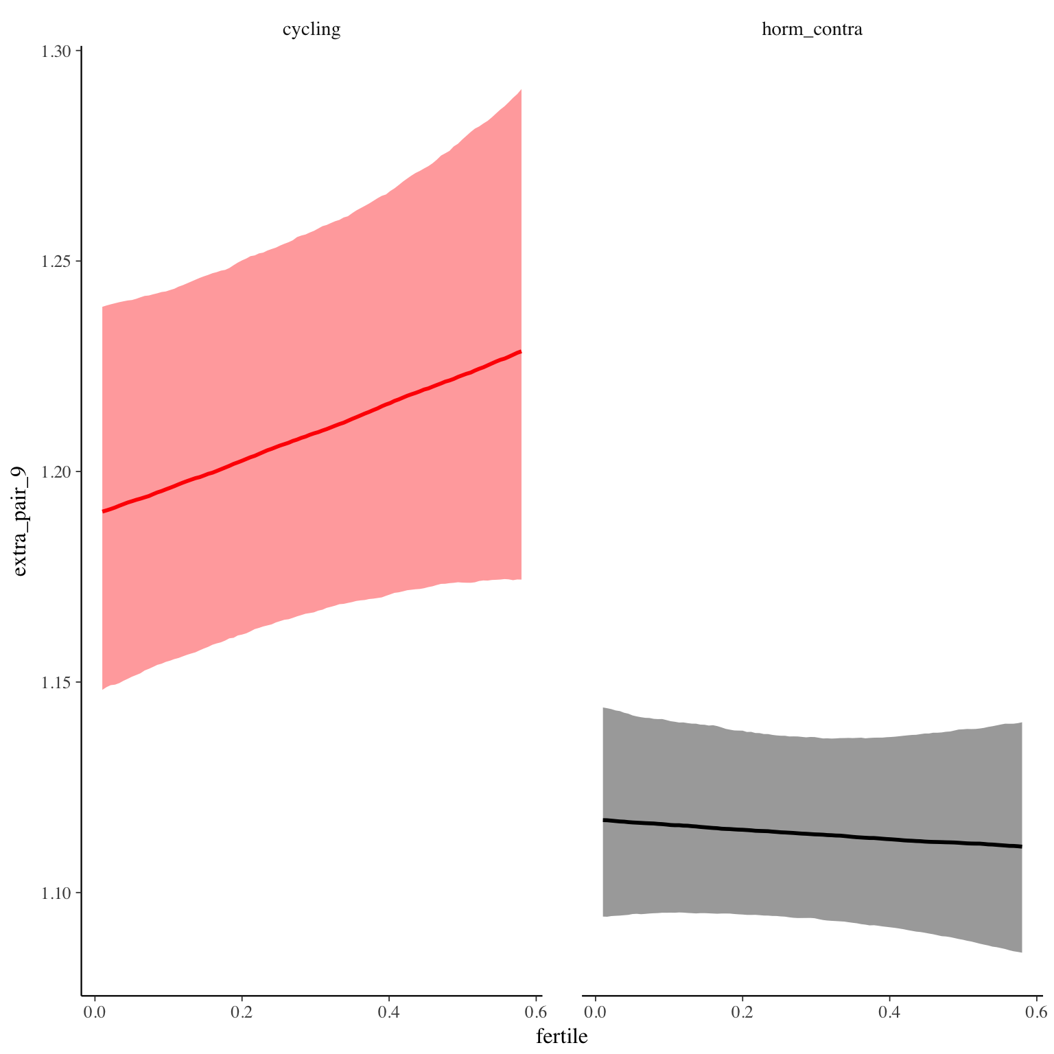
Diagnostics

extra_pair_intimacy_sex
Item text:
Item translation:
Choices:
| choice | value | frequency | percent |
|---|---|---|---|
| 0 | NA | 29467 | 0.99 |
| 1 | NA | 266 | 0.01 |
| 2 | NA | 134 | 0 |
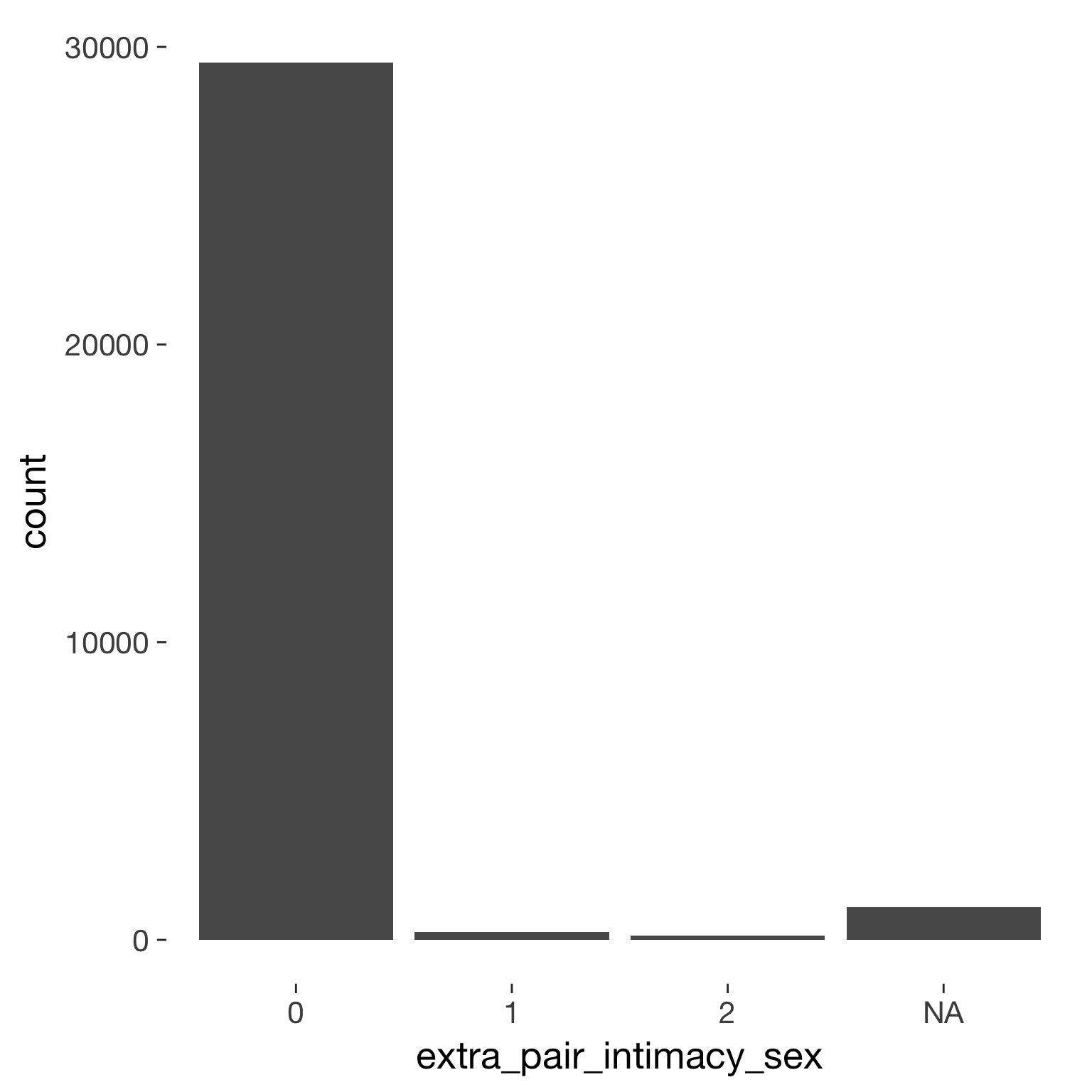
Model
Model summary
 Family: cumulative(logit)
Formula: extra_pair_intimacy_sex ~ included * (menstruation + fertile) + fertile_mean + (1 + fertile + menstruation | person)
         disc = 1
   Data: diary (Number of observations: 26567)
Samples: 4 chains, each with iter = 2000; warmup = 1000; thin = 1;
         total post-warmup samples = 4000
    ICs: LOO = 2813.33; WAIC = Not computed

Group-Level Effects:
~person (Number of levels: 1043)
                                     Estimate Est.Error l-95% CI u-95% CI Eff.Sample Rhat
sd(Intercept)                            2.93      0.28     2.42     3.52        857 1.00
sd(fertile)                              1.14      0.64     0.07     2.45        686 1.00
sd(menstruationpre)                      0.26      0.20     0.01     0.73       1972 1.00
sd(menstruationyes)                      0.57      0.35     0.03     1.31        598 1.01
cor(Intercept,fertile)                   0.21      0.33    -0.51     0.81       4000 1.00
cor(Intercept,menstruationpre)           0.05      0.44    -0.78     0.83       4000 1.00
cor(fertile,menstruationpre)             0.00      0.45    -0.80     0.81       4000 1.00
cor(Intercept,menstruationyes)           0.00      0.35    -0.71     0.67       4000 1.00
cor(fertile,menstruationyes)            -0.11      0.42    -0.84     0.71       1701 1.00
cor(menstruationpre,menstruationyes)     0.03      0.45    -0.80     0.83       1486 1.00

Population-Level Effects:
                                    Estimate Est.Error l-95% CI u-95% CI Eff.Sample Rhat
Intercept[1]                            6.85      0.49     5.91     7.86       1659    1
Intercept[2]                            8.28      0.50     7.33     9.31       1686    1
includedhorm_contra                    -1.28      0.38    -2.02    -0.55       1481    1
menstruationpre                        -0.09      0.32    -0.78     0.49       4000    1
menstruationyes                        -0.04      0.40    -0.90     0.70       3163    1
fertile                                -0.32      0.76    -2.04     0.95       1895    1
fertile_mean                           -0.82      1.33    -3.97     1.37       4000    1
includedhorm_contra:menstruationpre    -0.20      0.38    -0.97     0.54       4000    1
includedhorm_contra:menstruationyes    -0.07      0.37    -0.82     0.65       4000    1
includedhorm_contra:fertile            -0.24      0.65    -1.55     0.98       4000    1

Samples were drawn using sampling(NUTS). For each parameter, Eff.Sample
is a crude measure of effective sample size, and Rhat is the potential
scale reduction factor on split chains (at convergence, Rhat = 1).
Coefficient plot
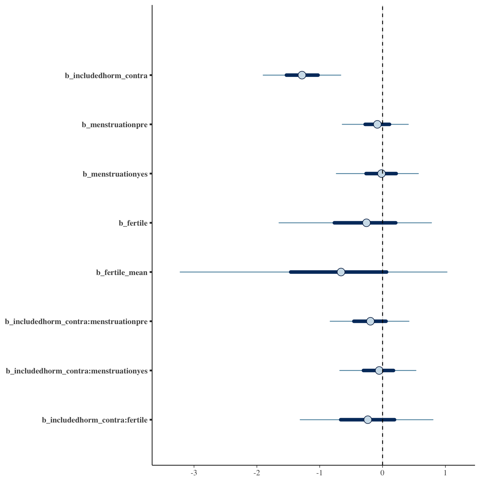
Marginal effect plots
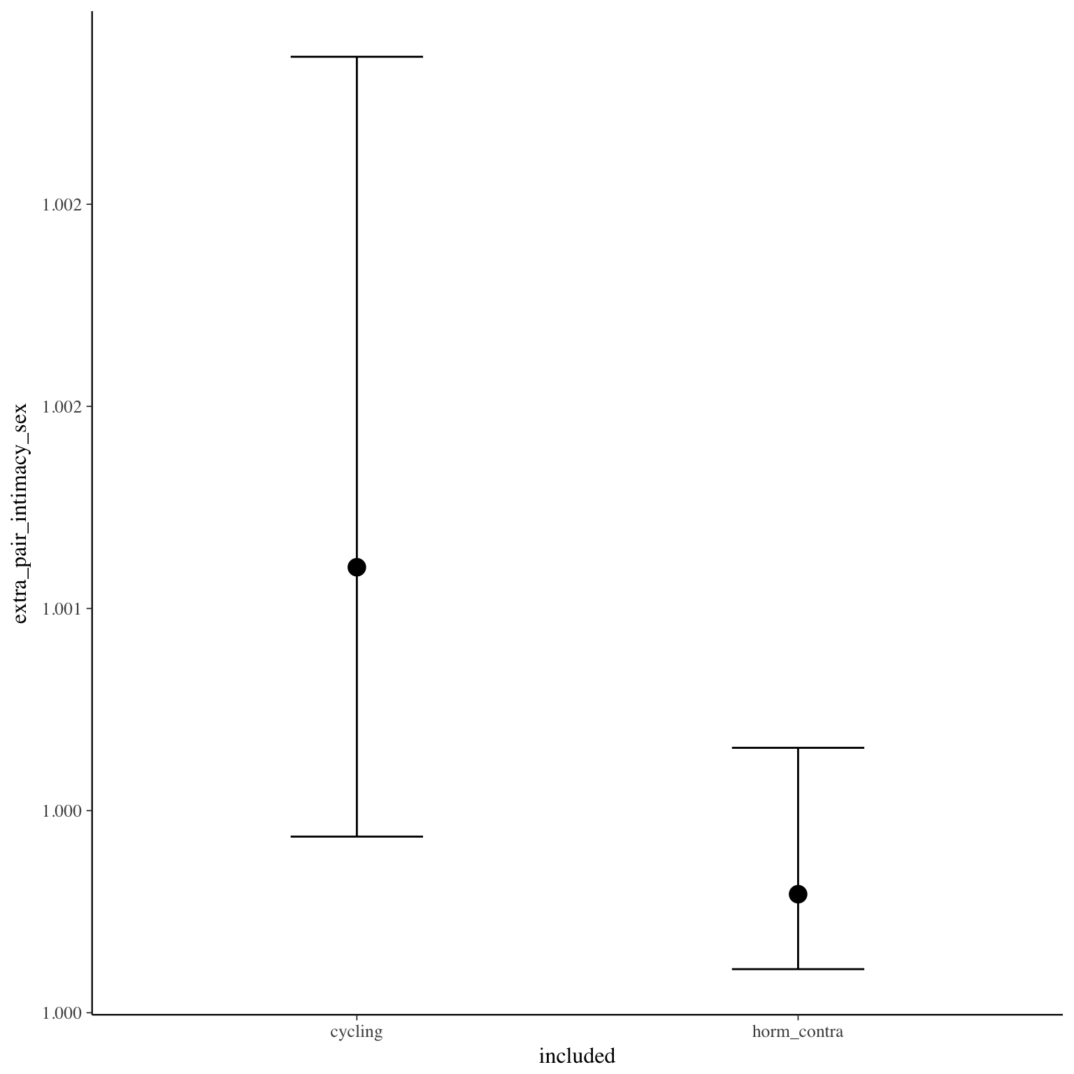
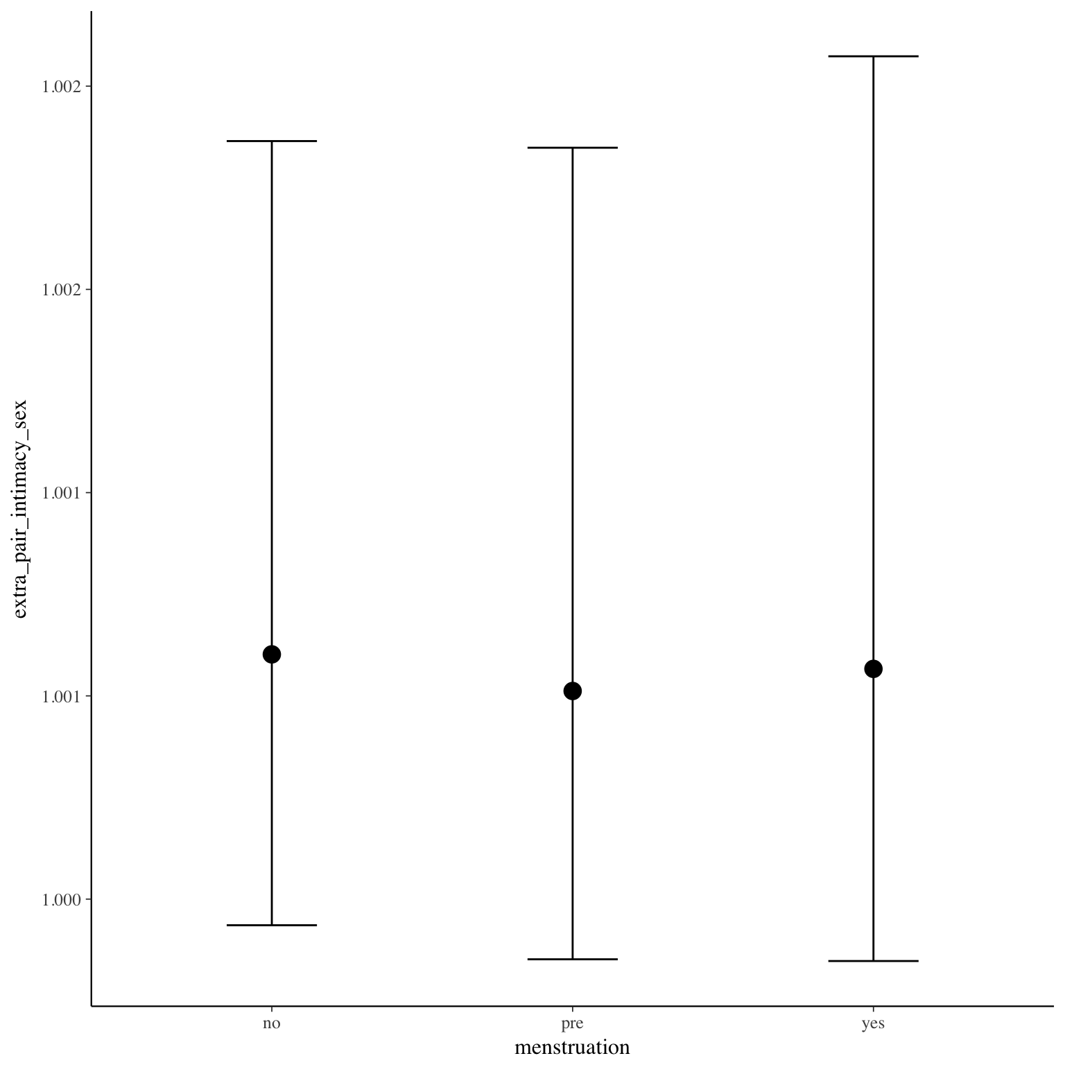
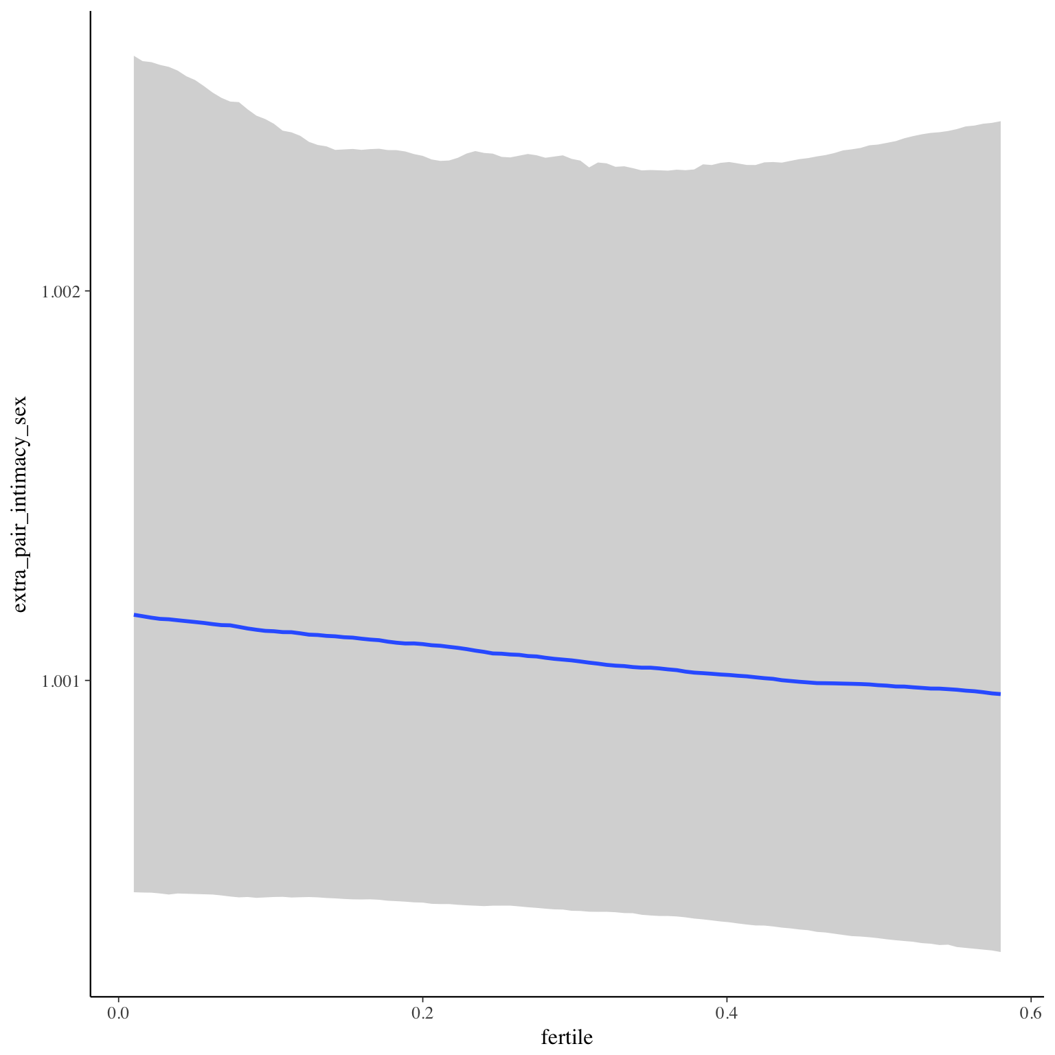
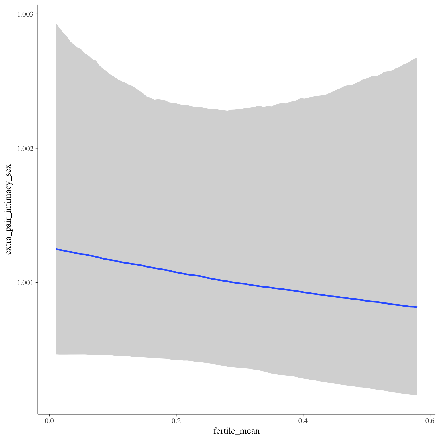
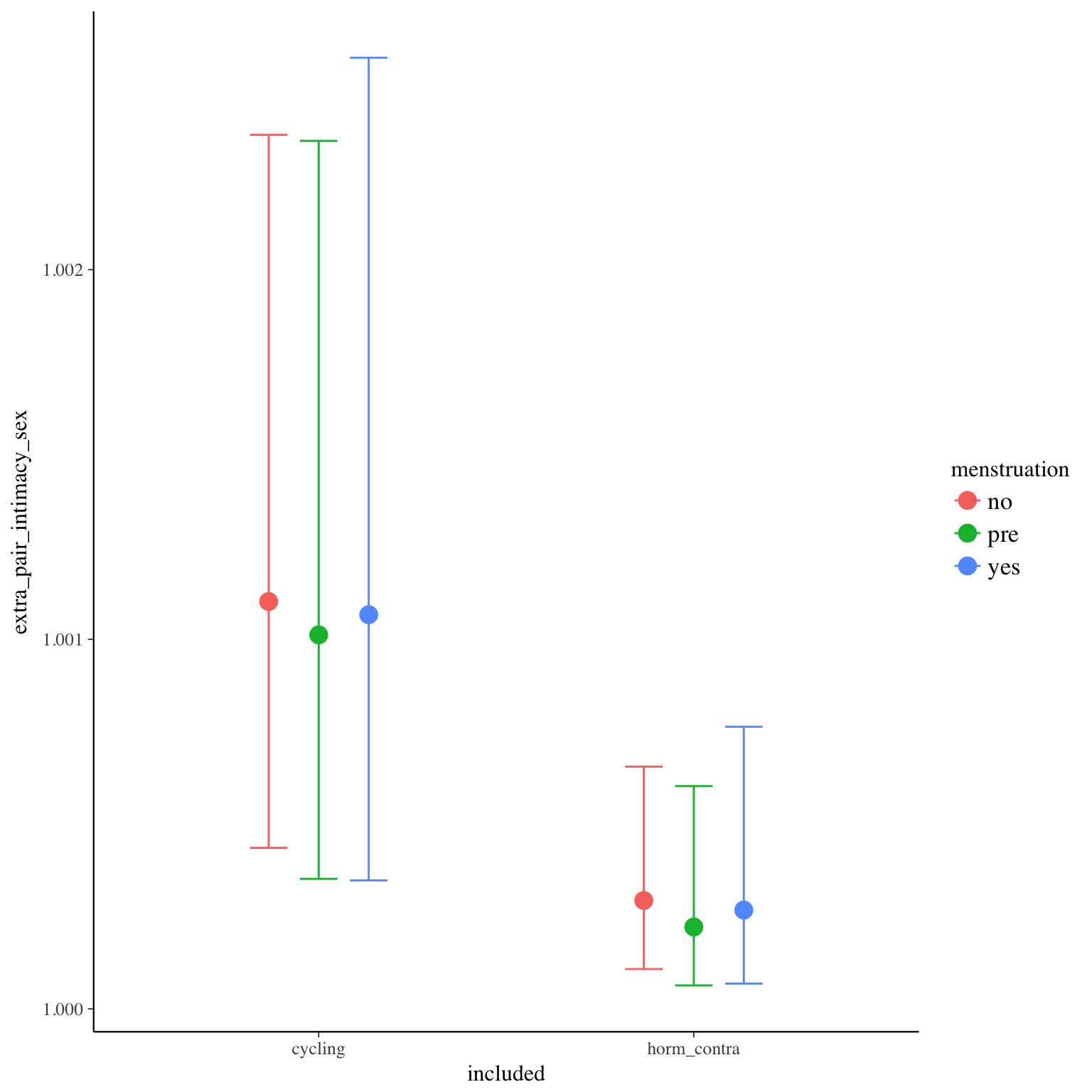
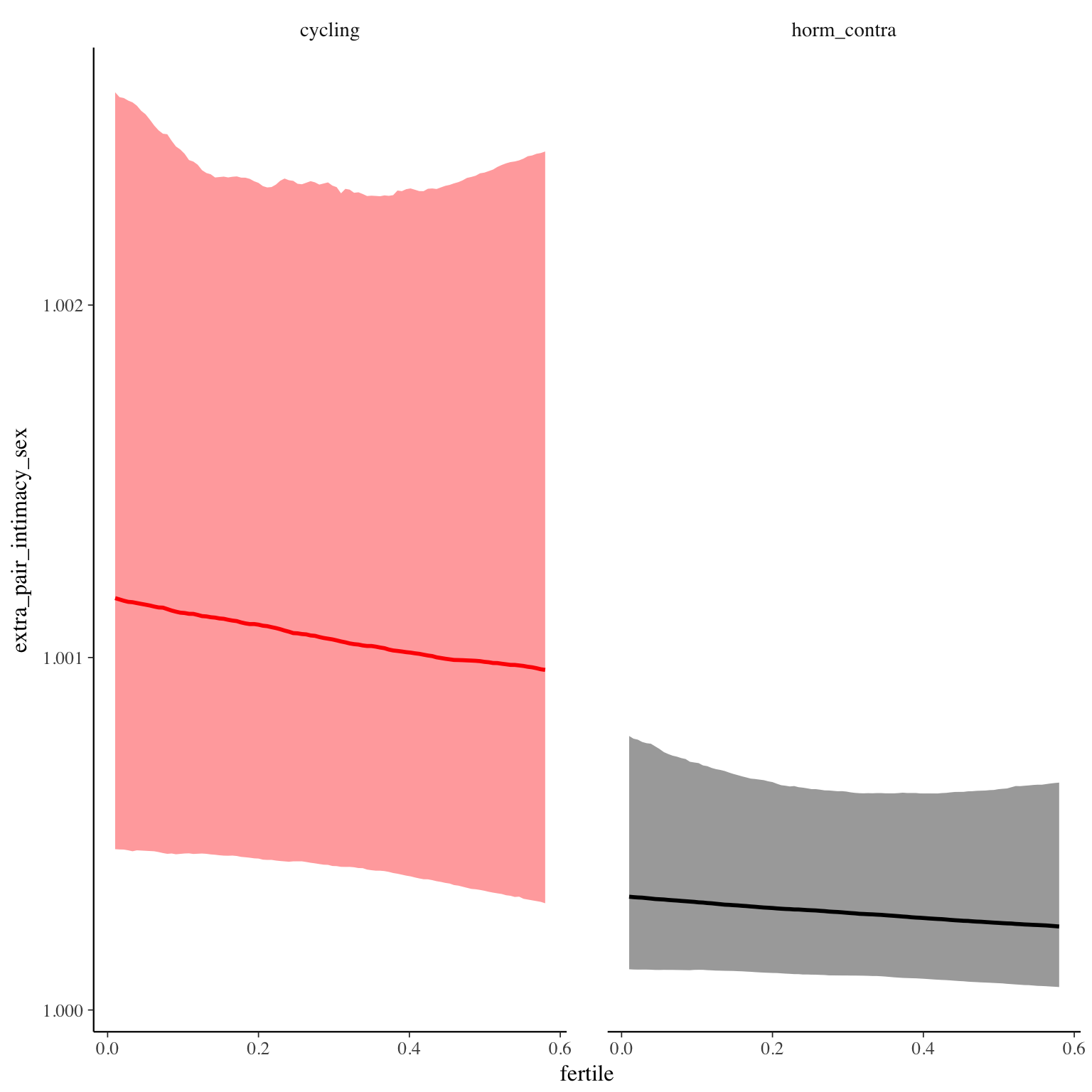
Diagnostics
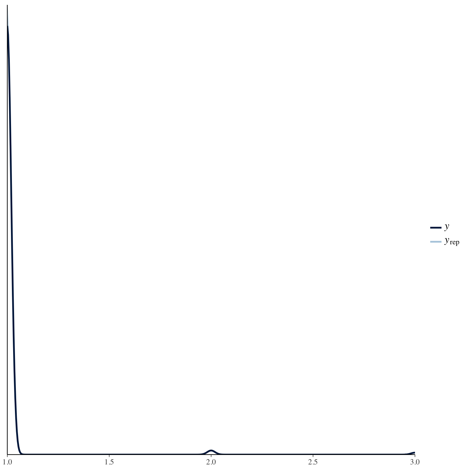
jealousy_1
Item text:
… habe ich meinen Partner gefragt, mit wem er den Tag verbracht hat.
Item translation:
33. I asked my partner with whom he spent the day.
Choices:
| choice | value | frequency | percent |
|---|---|---|---|
| 1 | Stimme nicht zu | 16788 | 0.56 |
| 2 | Stimme überwiegend nicht zu | 1826 | 0.06 |
| 3 | Stimme eher nicht zu | 2111 | 0.07 |
| 4 | Stimme eher zu | 3706 | 0.12 |
| 5 | Stimme überwiegend zu | 2333 | 0.08 |
| 6 | Stimme voll zu | 3113 | 0.1 |
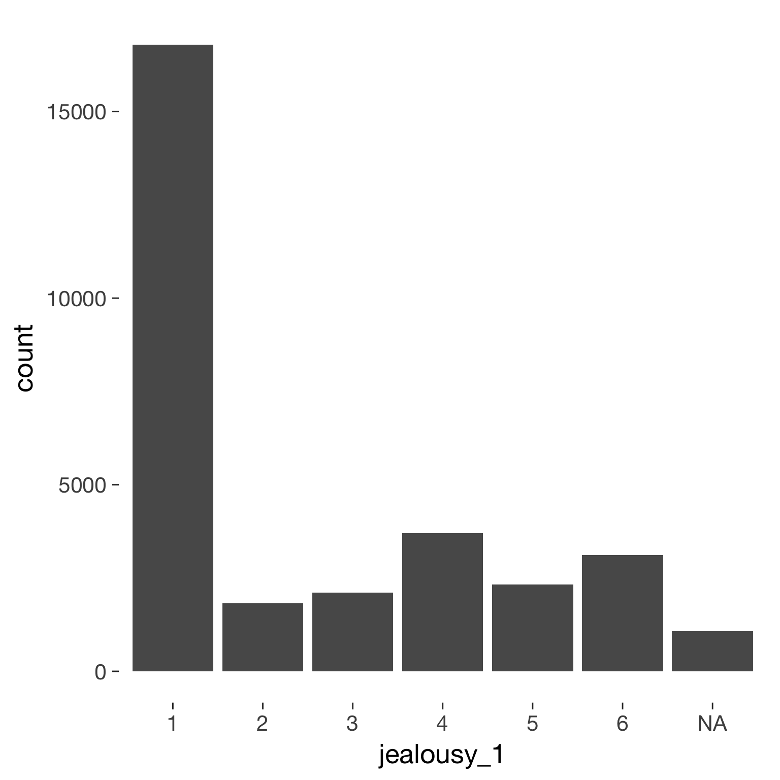
Model
Model summary
 Family: cumulative(logit)
Formula: jealousy_1 ~ included * (menstruation + fertile) + fertile_mean + (1 + fertile + menstruation | person)
         disc = 1
   Data: diary (Number of observations: 26546)
Samples: 4 chains, each with iter = 2000; warmup = 1000; thin = 1;
         total post-warmup samples = 4000
    ICs: LOO = 58931.67; WAIC = Not computed

Group-Level Effects:
~person (Number of levels: 1043)
                                     Estimate Est.Error l-95% CI u-95% CI Eff.Sample Rhat
sd(Intercept)                            2.10      0.07     1.97     2.23        593 1.00
sd(fertile)                              1.55      0.14     1.26     1.81        575 1.01
sd(menstruationpre)                      0.56      0.10     0.34     0.73        316 1.01
sd(menstruationyes)                      0.62      0.09     0.44     0.77        378 1.01
cor(Intercept,fertile)                  -0.03      0.09    -0.21     0.15       2098 1.00
cor(Intercept,menstruationpre)           0.20      0.13    -0.06     0.47        776 1.01
cor(fertile,menstruationpre)             0.14      0.17    -0.25     0.43        359 1.02
cor(Intercept,menstruationyes)           0.10      0.12    -0.13     0.34       1612 1.00
cor(fertile,menstruationyes)             0.32      0.13     0.04     0.56        542 1.01
cor(menstruationpre,menstruationyes)     0.43      0.17     0.05     0.73        271 1.02

Population-Level Effects:
                                    Estimate Est.Error l-95% CI u-95% CI Eff.Sample Rhat
Intercept[1]                            0.37      0.17     0.03     0.69        546 1.00
Intercept[2]                            0.80      0.17     0.46     1.12        544 1.00
Intercept[3]                            1.30      0.17     0.96     1.63        544 1.00
Intercept[4]                            2.37      0.17     2.03     2.69        548 1.00
Intercept[5]                            3.35      0.17     3.01     3.68        558 1.00
includedhorm_contra                     0.19      0.14    -0.08     0.46        360 1.01
menstruationpre                        -0.12      0.09    -0.29     0.04       1831 1.00
menstruationyes                        -0.10      0.08    -0.26     0.06       2033 1.00
fertile                                -0.03      0.18    -0.38     0.32       1915 1.00
fertile_mean                           -0.94      0.75    -2.50     0.41        789 1.00
includedhorm_contra:menstruationpre     0.08      0.10    -0.12     0.27       1961 1.00
includedhorm_contra:menstruationyes     0.08      0.10    -0.11     0.28       2193 1.00
includedhorm_contra:fertile             0.09      0.21    -0.32     0.50       2121 1.00

Samples were drawn using sampling(NUTS). For each parameter, Eff.Sample
is a crude measure of effective sample size, and Rhat is the potential
scale reduction factor on split chains (at convergence, Rhat = 1).
Coefficient plot
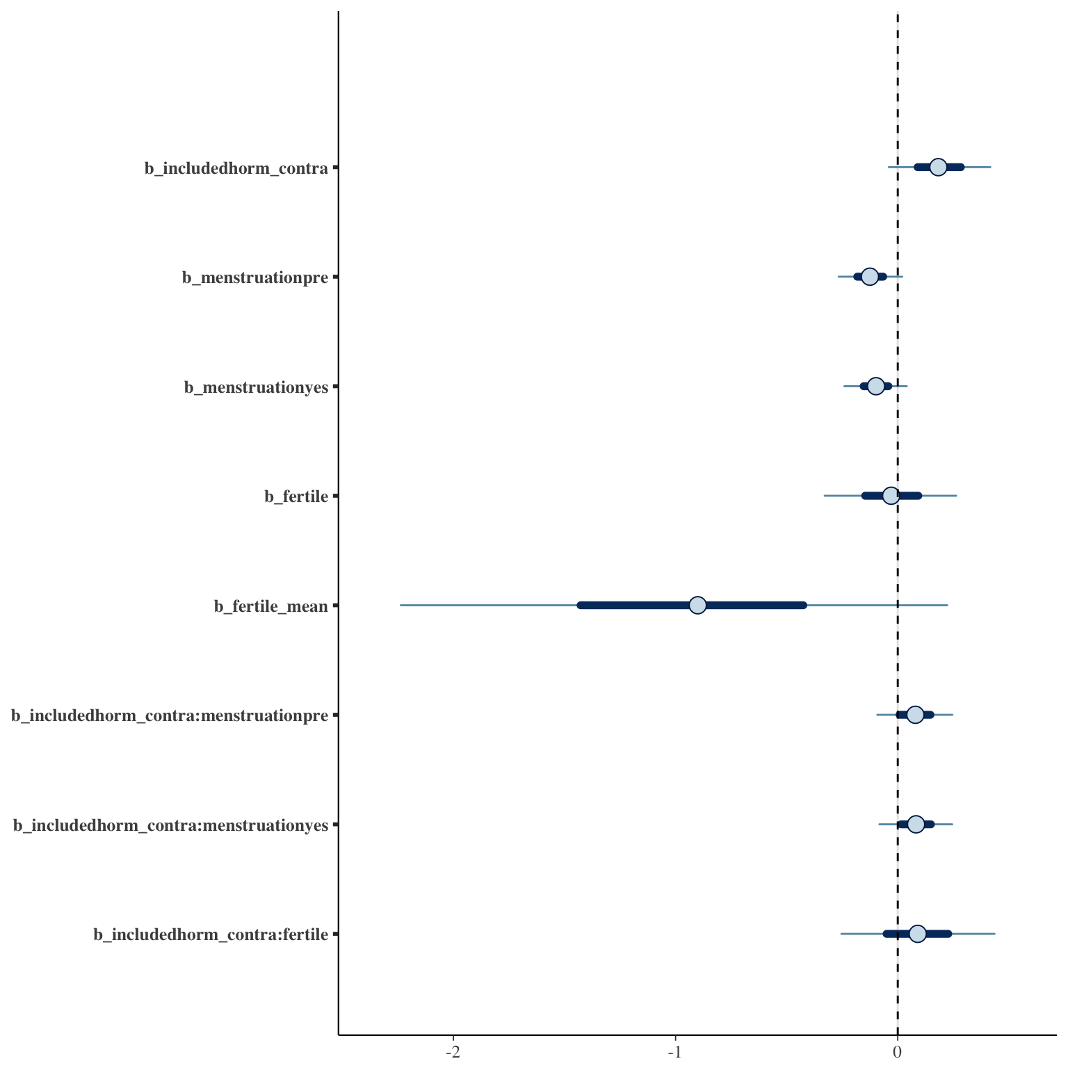
Marginal effect plots
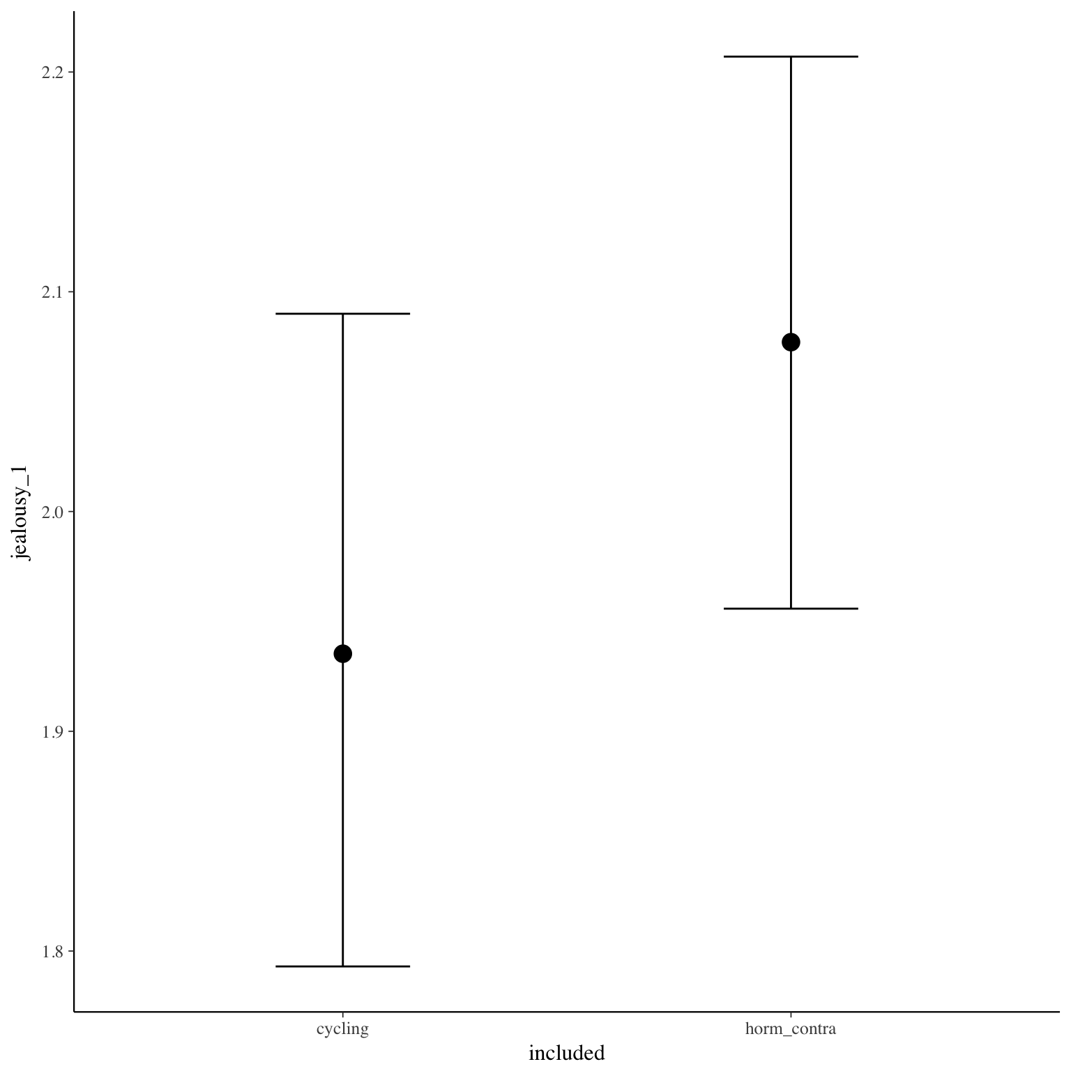
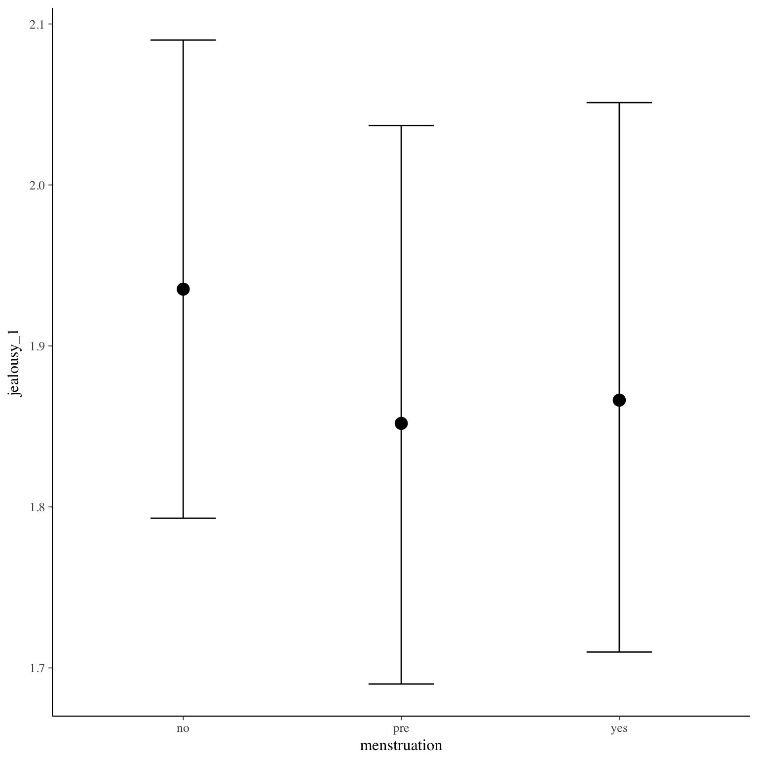
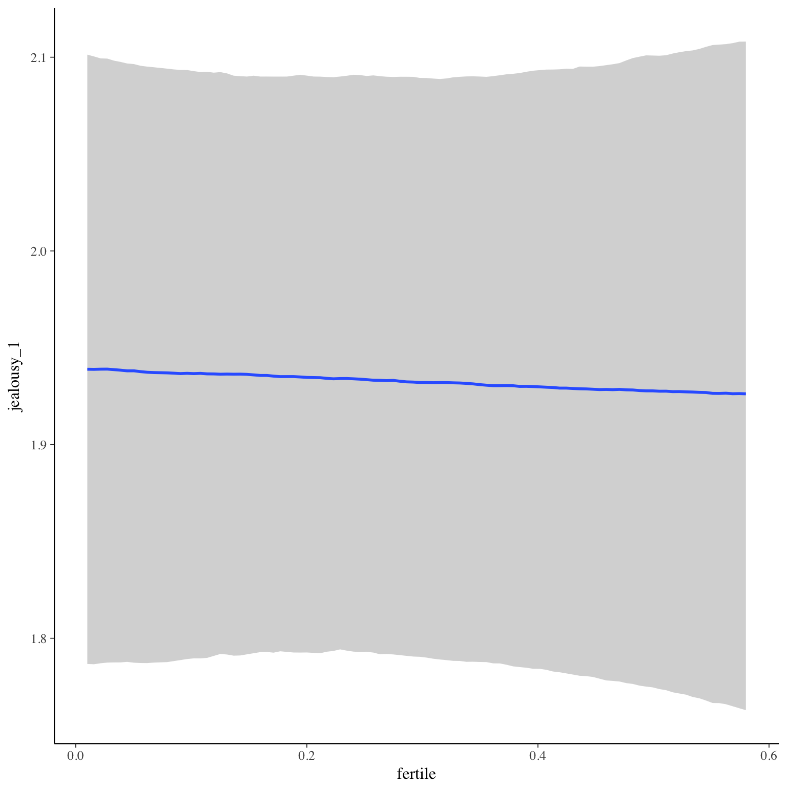
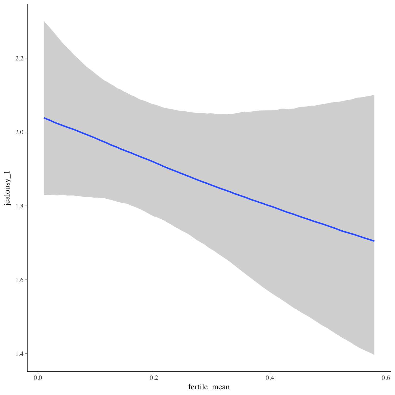
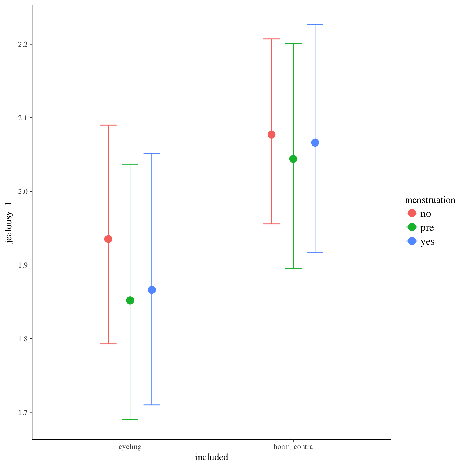
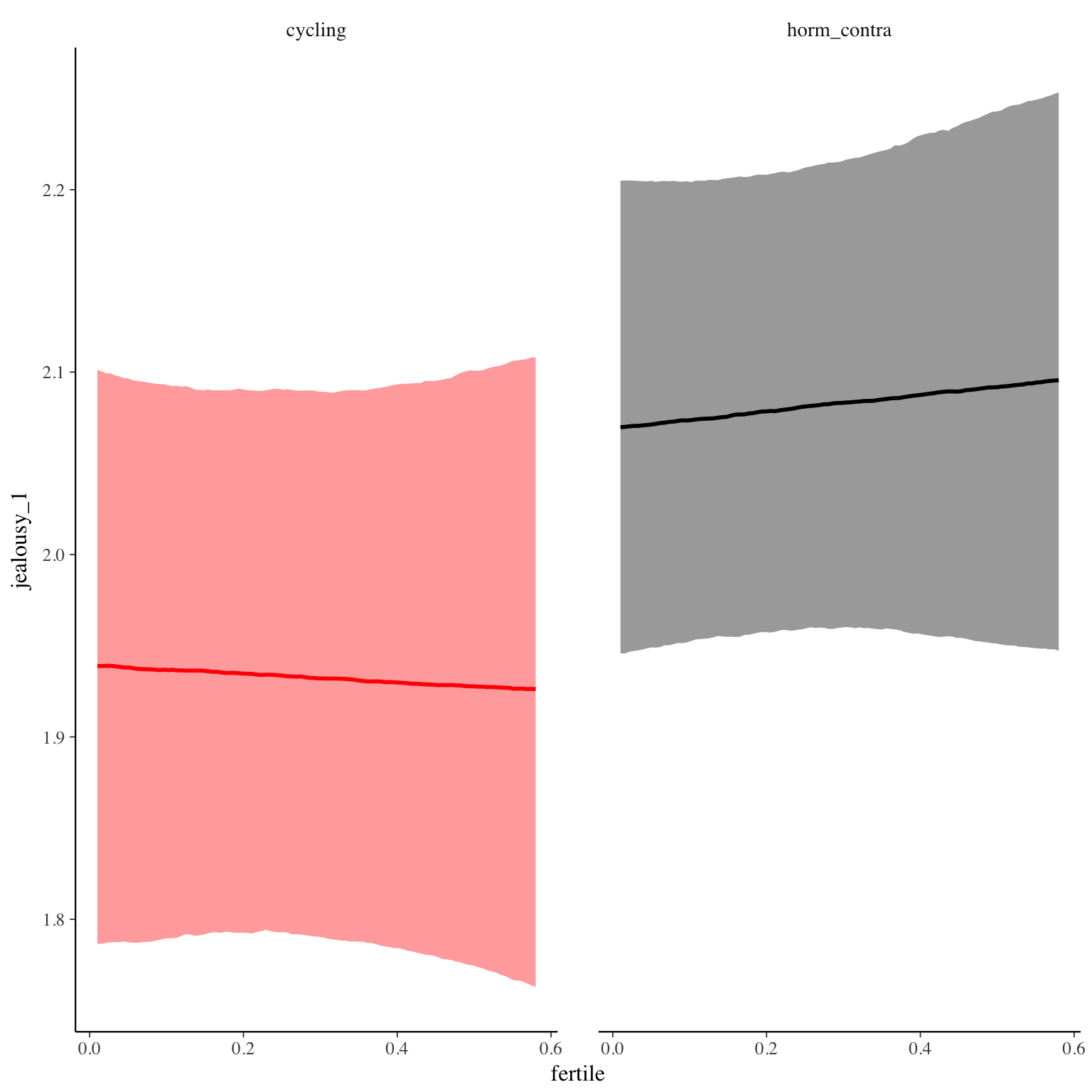
Diagnostics
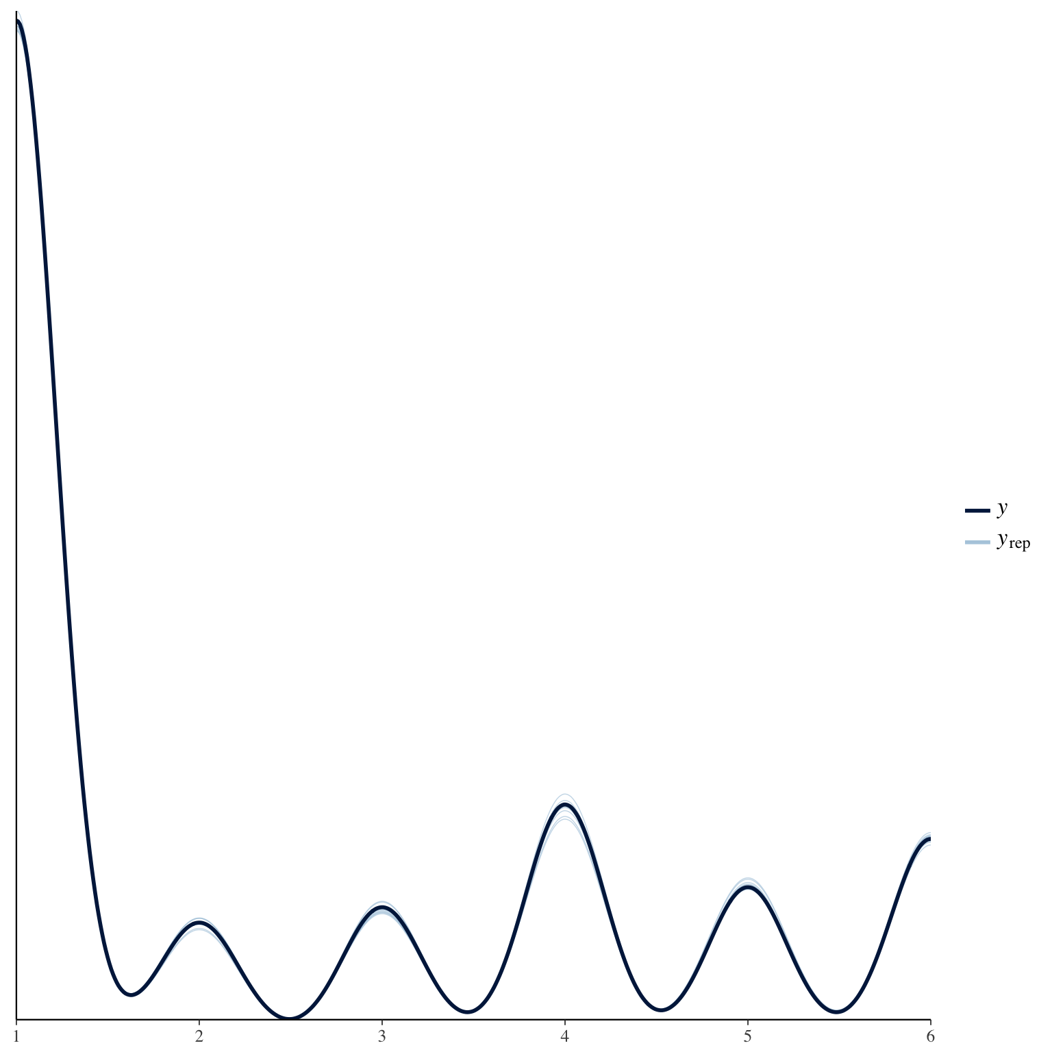
male_attention_1
Item text:
… hat mir mein Partner gezeigt, dass er sich von mir sexuell angezogen fühlt.
Item translation:
45. My partner showed me that he was sexually attracted to me.
Choices:
| choice | value | frequency | percent |
|---|---|---|---|
| 1 | Stimme nicht zu | 7147 | 0.24 |
| 2 | Stimme überwiegend nicht zu | 2601 | 0.09 |
| 3 | Stimme eher nicht zu | 3986 | 0.13 |
| 4 | Stimme eher zu | 5240 | 0.18 |
| 5 | Stimme überwiegend zu | 4890 | 0.16 |
| 6 | Stimme voll zu | 6010 | 0.2 |
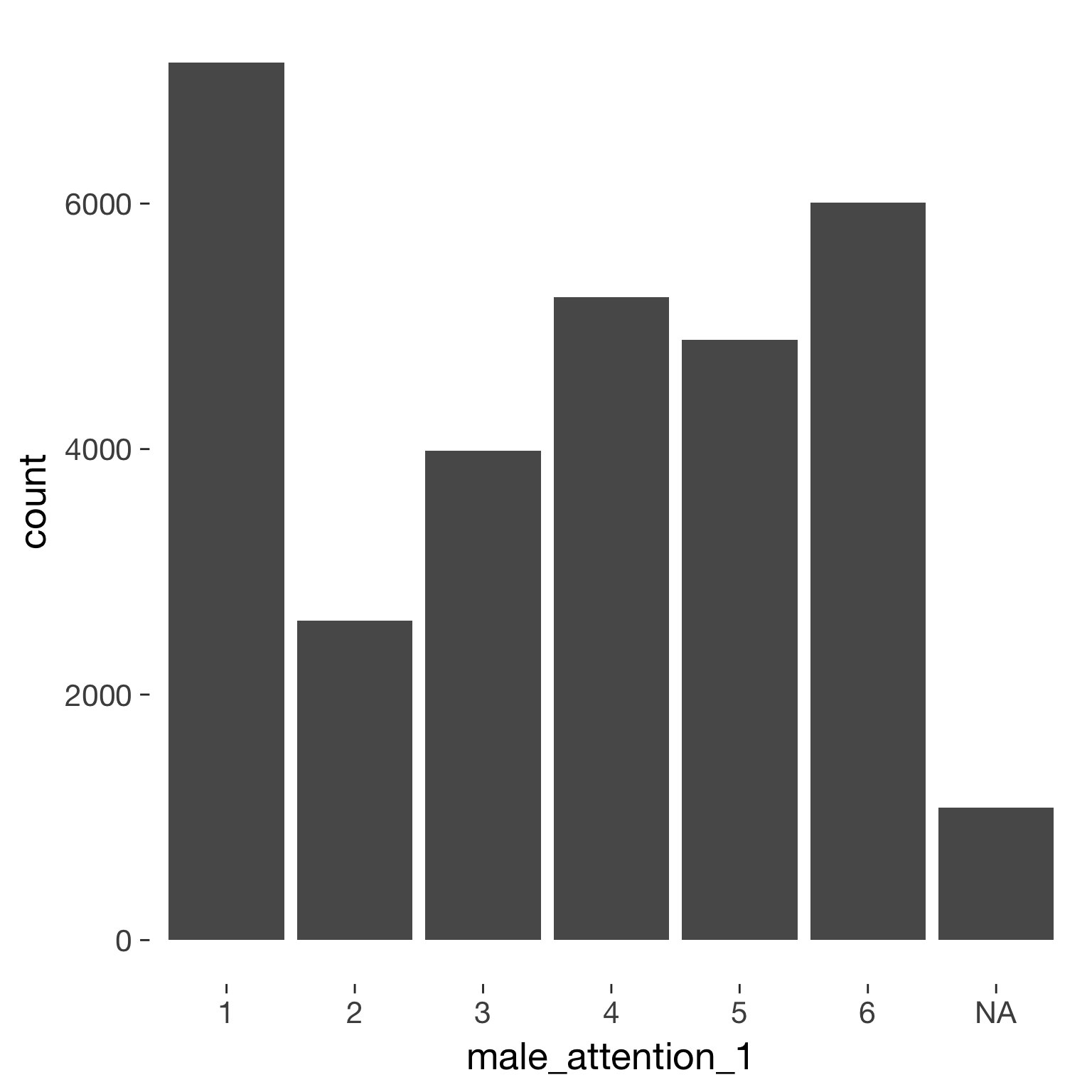
Model
Model summary
 Family: cumulative(logit)
Formula: male_attention_1 ~ included * (menstruation + fertile) + fertile_mean + (1 + fertile + menstruation | person)
         disc = 1
   Data: diary (Number of observations: 26544)
Samples: 4 chains, each with iter = 2000; warmup = 1000; thin = 1;
         total post-warmup samples = 4000
    ICs: LOO = 84166.42; WAIC = Not computed

Group-Level Effects:
~person (Number of levels: 1043)
                                     Estimate Est.Error l-95% CI u-95% CI Eff.Sample Rhat
sd(Intercept)                            1.38      0.04     1.30     1.47       1000 1.01
sd(fertile)                              1.65      0.11     1.43     1.87        824 1.01
sd(menstruationpre)                      0.73      0.06     0.61     0.85        711 1.01
sd(menstruationyes)                      0.71      0.06     0.60     0.82        818 1.00
cor(Intercept,fertile)                  -0.27      0.06    -0.39    -0.14       1741 1.01
cor(Intercept,menstruationpre)          -0.30      0.07    -0.43    -0.16       1782 1.01
cor(fertile,menstruationpre)             0.53      0.08     0.38     0.67        729 1.01
cor(Intercept,menstruationyes)          -0.32      0.07    -0.45    -0.19       1831 1.00
cor(fertile,menstruationyes)             0.40      0.09     0.22     0.56        655 1.00
cor(menstruationpre,menstruationyes)     0.51      0.09     0.33     0.67        693 1.00

Population-Level Effects:
                                    Estimate Est.Error l-95% CI u-95% CI Eff.Sample Rhat
Intercept[1]                           -1.43      0.12    -1.66    -1.20        839 1.01
Intercept[2]                           -0.85      0.12    -1.09    -0.63        842 1.01
Intercept[3]                           -0.10      0.12    -0.34     0.12        843 1.01
Intercept[4]                            0.81      0.12     0.58     1.04        851 1.00
Intercept[5]                            1.83      0.12     1.61     2.06        865 1.00
includedhorm_contra                     0.23      0.10     0.03     0.43        626 1.01
menstruationpre                        -0.05      0.07    -0.19     0.09       1539 1.00
menstruationyes                        -0.20      0.07    -0.33    -0.07       1487 1.00
fertile                                 0.15      0.15    -0.15     0.44       1573 1.00
fertile_mean                            0.09      0.50    -0.87     1.08       1613 1.00
includedhorm_contra:menstruationpre    -0.06      0.09    -0.25     0.11       1518 1.00
includedhorm_contra:menstruationyes    -0.03      0.09    -0.20     0.14       1594 1.00
includedhorm_contra:fertile            -0.48      0.19    -0.84    -0.12       1533 1.00

Samples were drawn using sampling(NUTS). For each parameter, Eff.Sample
is a crude measure of effective sample size, and Rhat is the potential
scale reduction factor on split chains (at convergence, Rhat = 1).
Coefficient plot
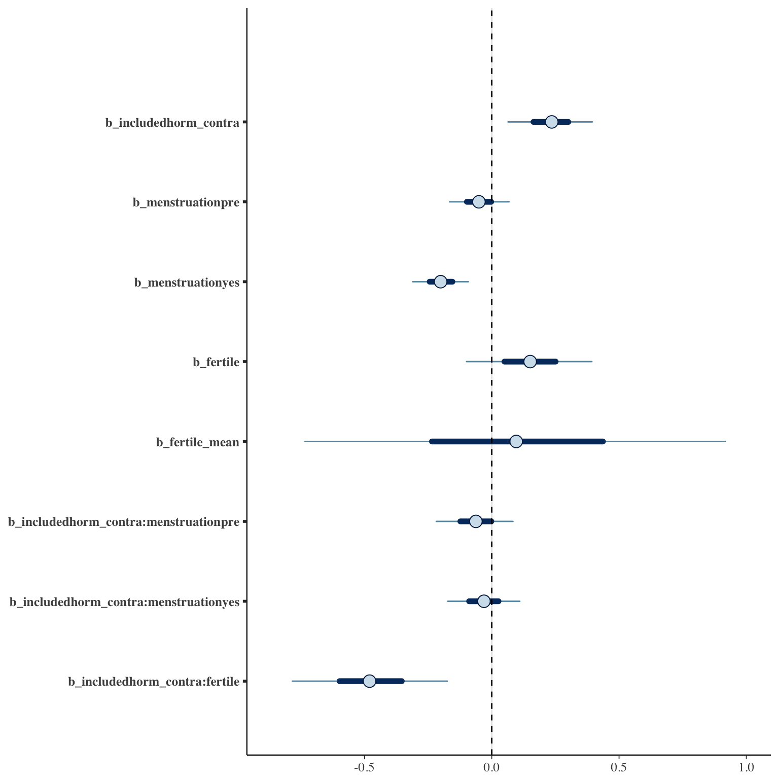
Marginal effect plots

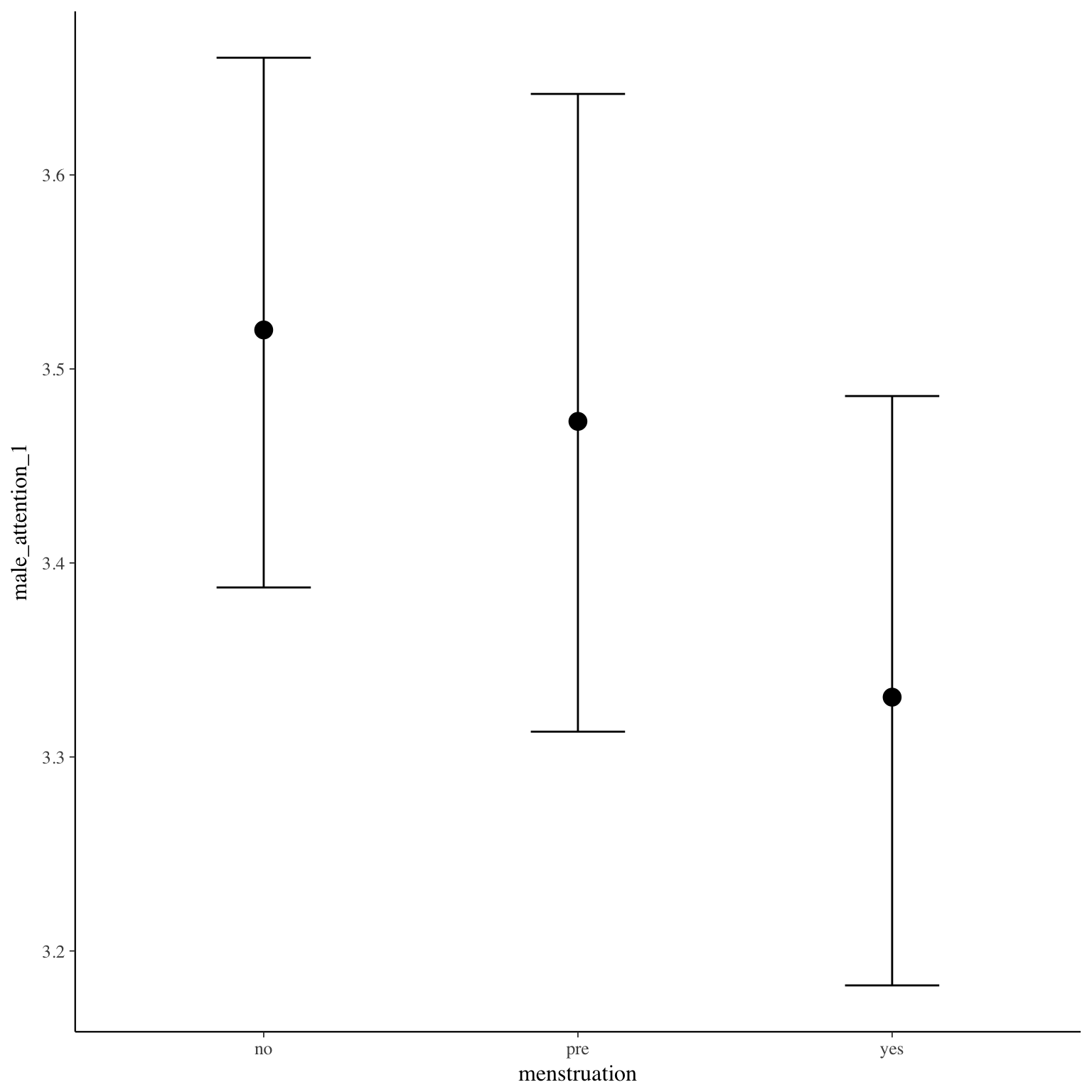
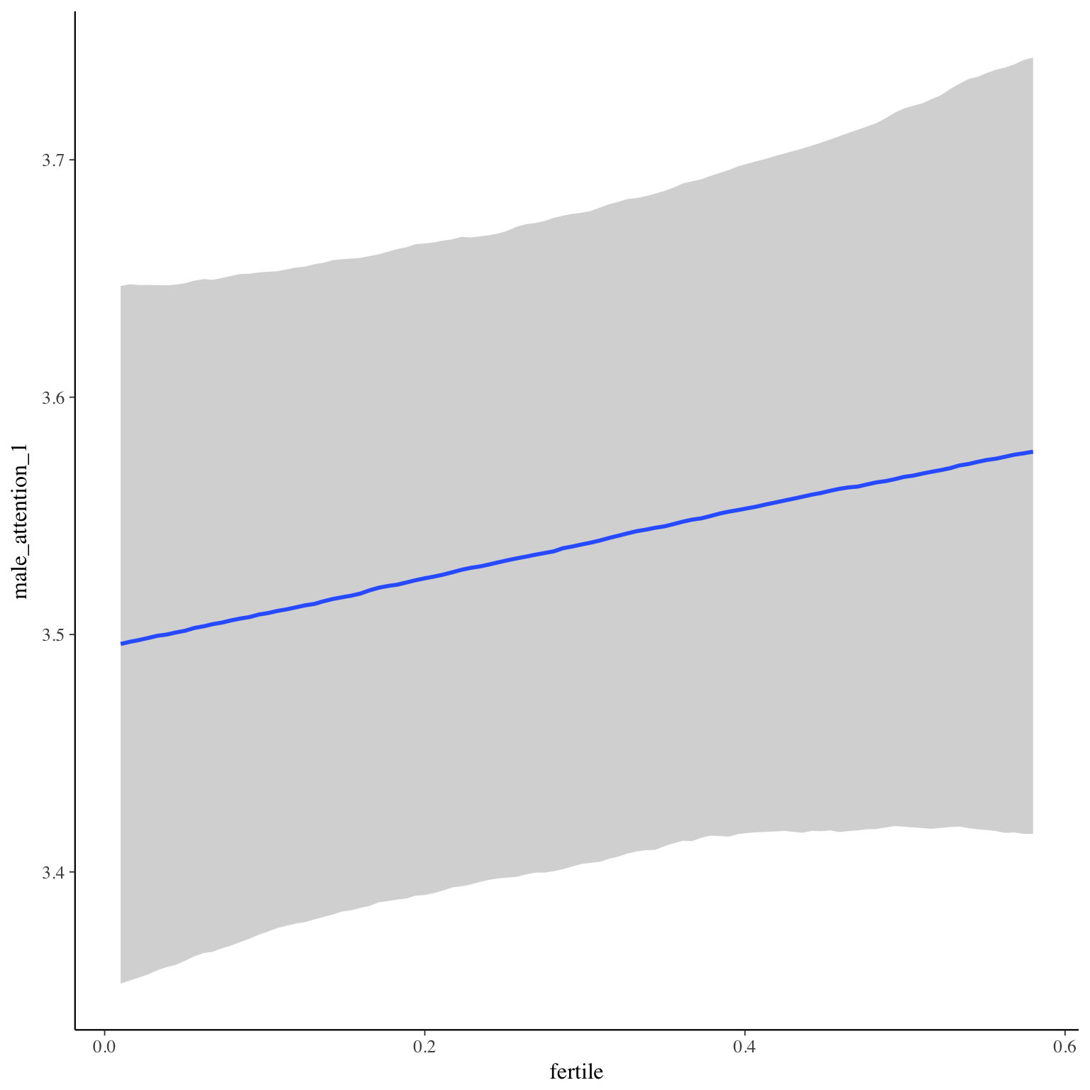
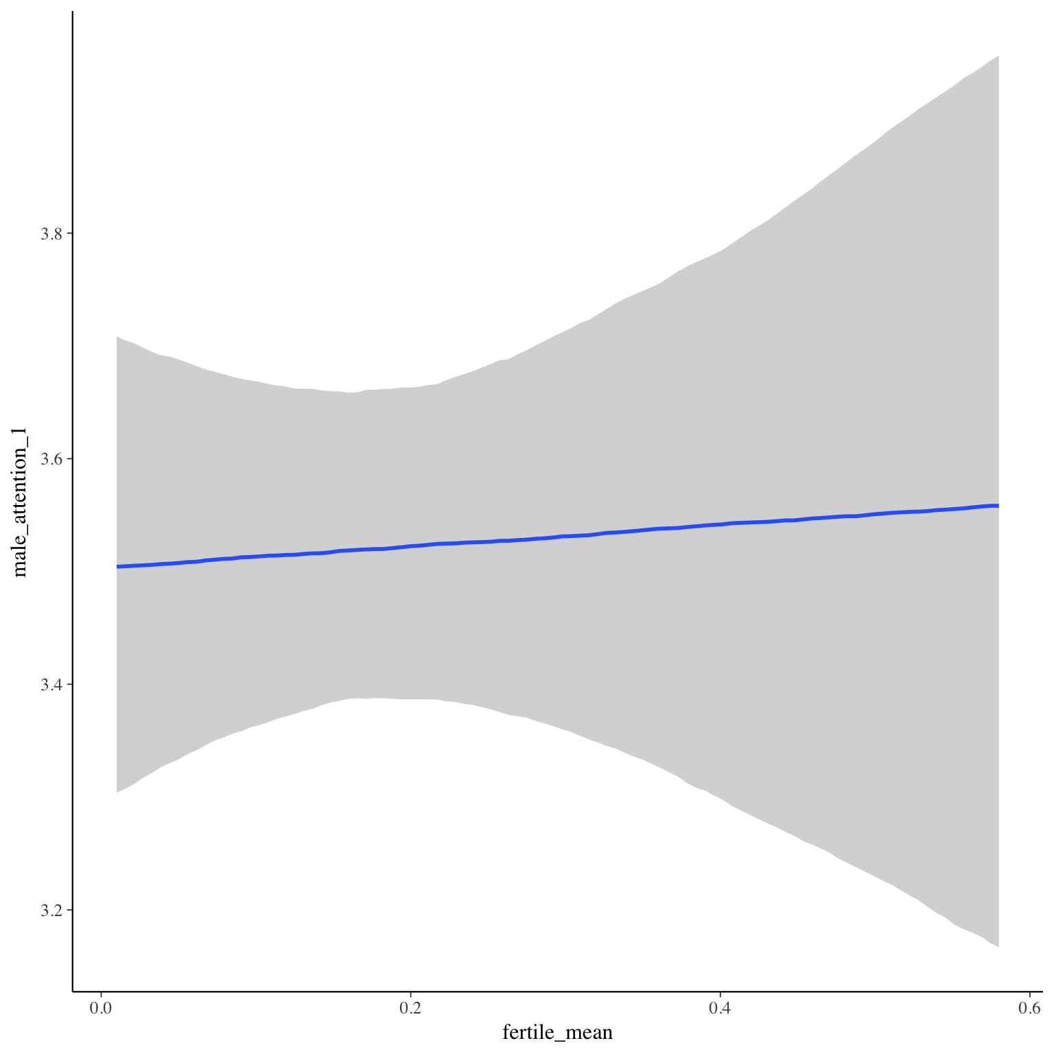
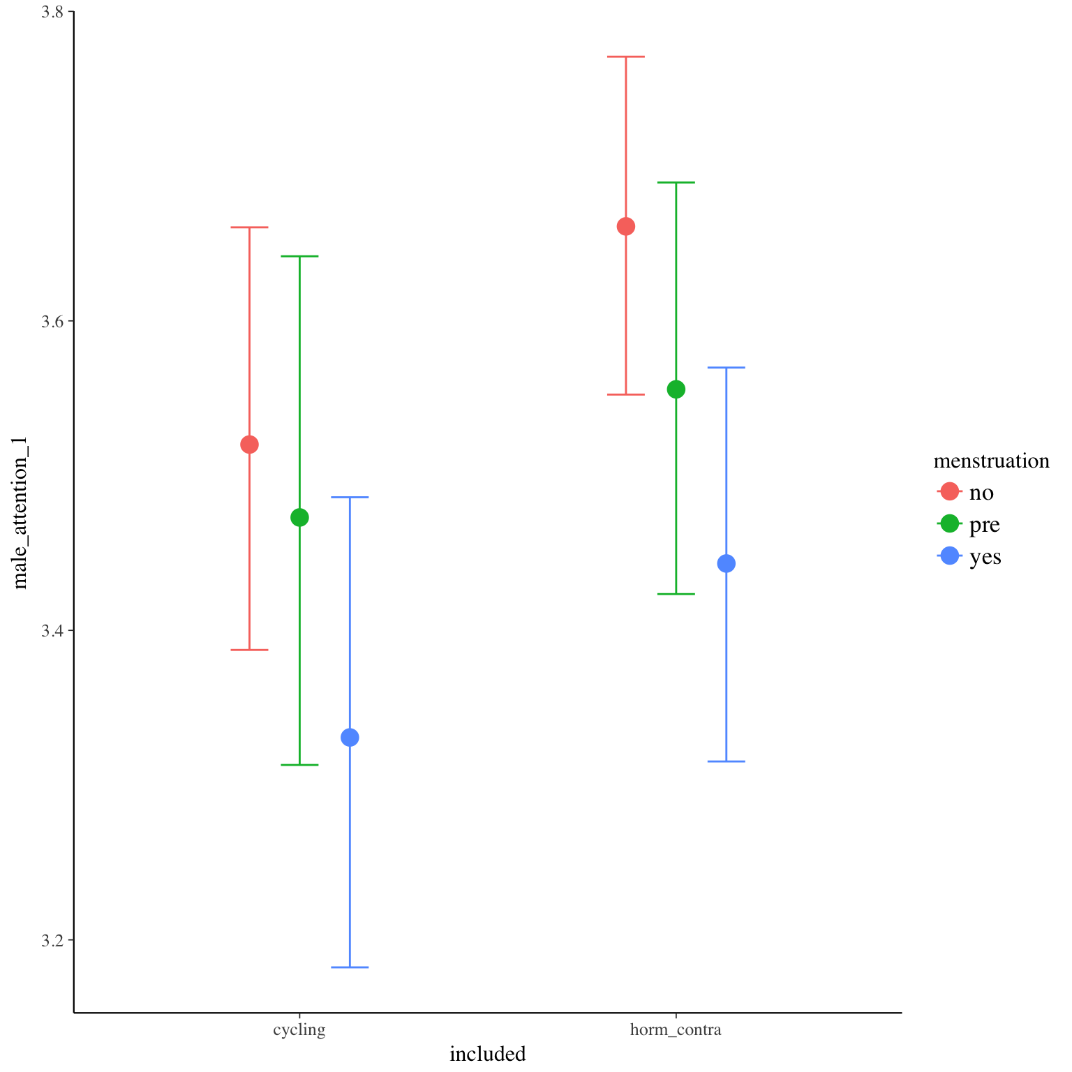
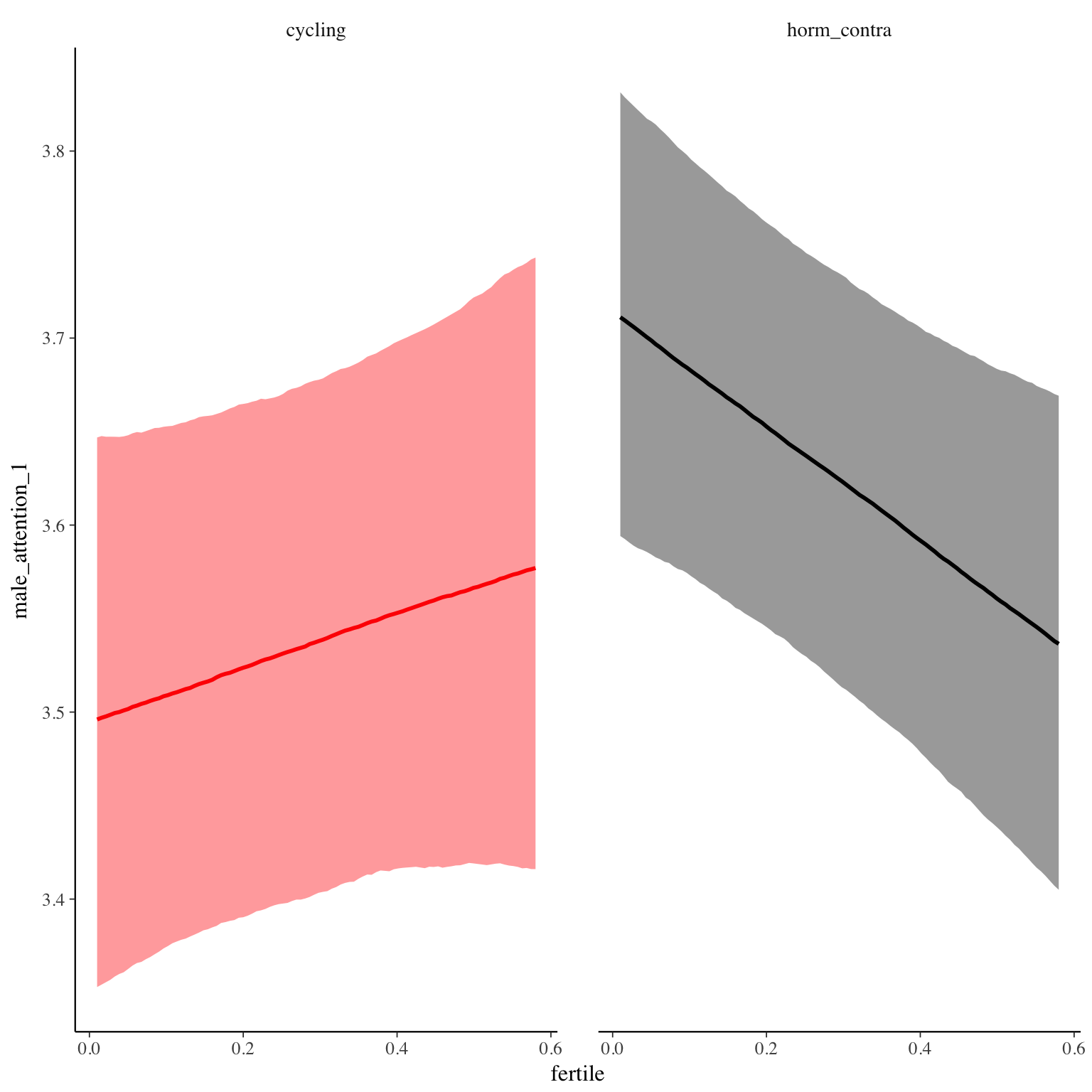
Diagnostics
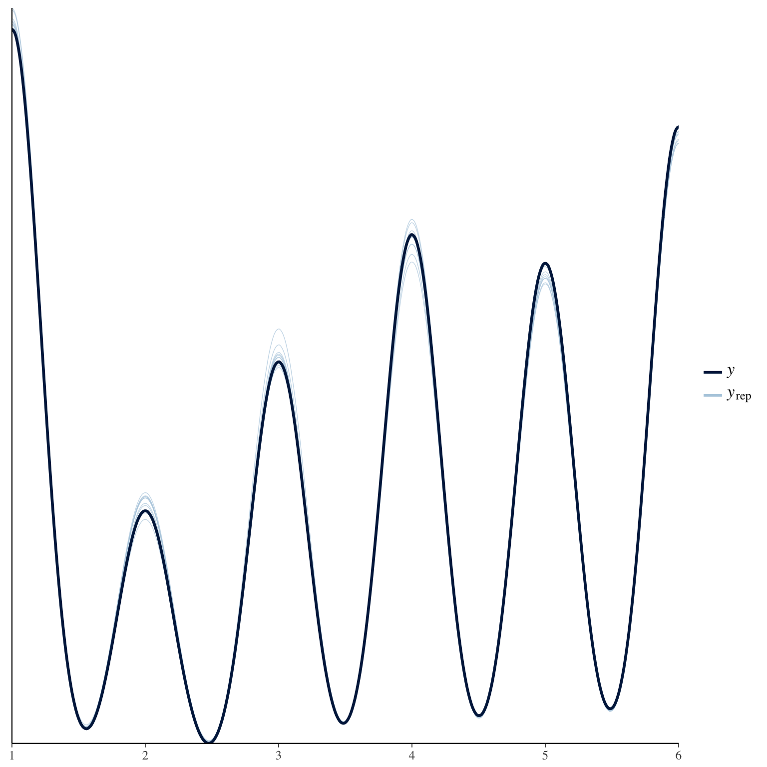
male_jealousy_1
Item text:
… hat mich mein Partner eifersüchtig gemacht.
Item translation:
34. My partner made me jealous.
Choices:
| choice | value | frequency | percent |
|---|---|---|---|
| 1 | Stimme nicht zu | 24376 | 0.82 |
| 2 | Stimme überwiegend nicht zu | 2162 | 0.07 |
| 3 | Stimme eher nicht zu | 1432 | 0.05 |
| 4 | Stimme eher zu | 1209 | 0.04 |
| 5 | Stimme überwiegend zu | 429 | 0.01 |
| 6 | Stimme voll zu | 268 | 0.01 |
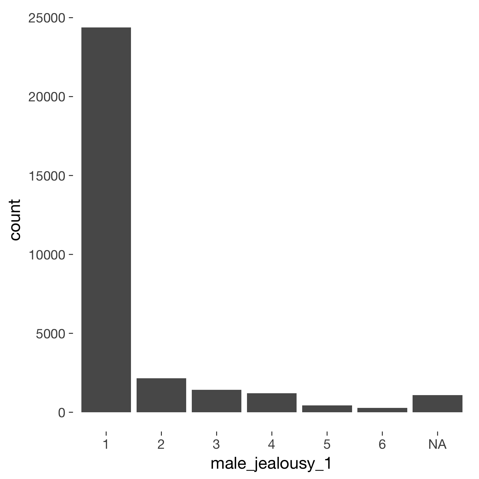
Model
Model summary
 Family: cumulative(logit)
Formula: male_jealousy_1 ~ included * (menstruation + fertile) + fertile_mean + (1 + fertile + menstruation | person)
         disc = 1
   Data: diary (Number of observations: 26545)
Samples: 4 chains, each with iter = 2000; warmup = 1000; thin = 1;
         total post-warmup samples = 4000
    ICs: LOO = 33123.36; WAIC = Not computed

Group-Level Effects:
~person (Number of levels: 1043)
                                     Estimate Est.Error l-95% CI u-95% CI Eff.Sample Rhat
sd(Intercept)                            1.81      0.07     1.67     1.96       1100 1.00
sd(fertile)                              1.61      0.19     1.24     1.98        484 1.01
sd(menstruationpre)                      0.54      0.16     0.19     0.81        255 1.02
sd(menstruationyes)                      0.39      0.18     0.03     0.70        213 1.03
cor(Intercept,fertile)                  -0.24      0.10    -0.43    -0.03       3127 1.00
cor(Intercept,menstruationpre)           0.07      0.17    -0.25     0.42       2451 1.00
cor(fertile,menstruationpre)            -0.05      0.26    -0.64     0.37        367 1.01
cor(Intercept,menstruationyes)          -0.07      0.24    -0.58     0.46       3276 1.00
cor(fertile,menstruationyes)             0.04      0.30    -0.66     0.55        603 1.01
cor(menstruationpre,menstruationyes)     0.26      0.34    -0.56     0.81        453 1.01

Population-Level Effects:
                                    Estimate Est.Error l-95% CI u-95% CI Eff.Sample Rhat
Intercept[1]                            2.62      0.16     2.32     2.94       1402    1
Intercept[2]                            3.42      0.16     3.11     3.74       1431    1
Intercept[3]                            4.17      0.16     3.87     4.50       1471    1
Intercept[4]                            5.36      0.17     5.04     5.70       1534    1
Intercept[5]                            6.41      0.17     6.07     6.76       1646    1
includedhorm_contra                     0.44      0.14     0.15     0.71        879    1
menstruationpre                        -0.09      0.13    -0.34     0.16       2315    1
menstruationyes                        -0.01      0.11    -0.23     0.20       2682    1
fertile                                 0.19      0.24    -0.29     0.66       3154    1
fertile_mean                            0.41      0.64    -0.84     1.73       2130    1
includedhorm_contra:menstruationpre     0.10      0.13    -0.15     0.35       4000    1
includedhorm_contra:menstruationyes     0.04      0.12    -0.18     0.27       4000    1
includedhorm_contra:fertile            -0.04      0.25    -0.52     0.47       4000    1

Samples were drawn using sampling(NUTS). For each parameter, Eff.Sample
is a crude measure of effective sample size, and Rhat is the potential
scale reduction factor on split chains (at convergence, Rhat = 1).
Coefficient plot
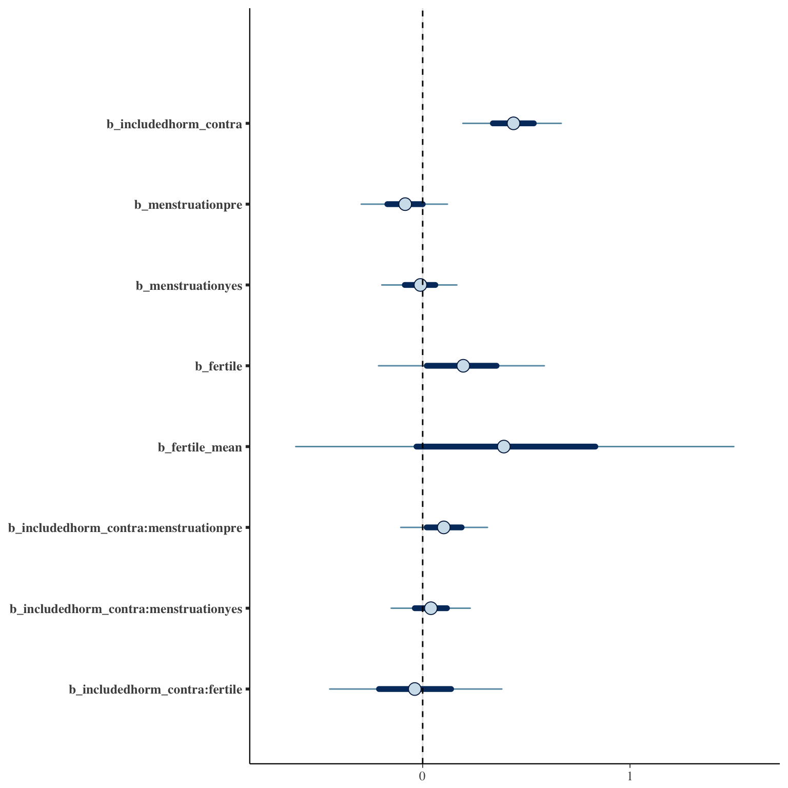
Marginal effect plots
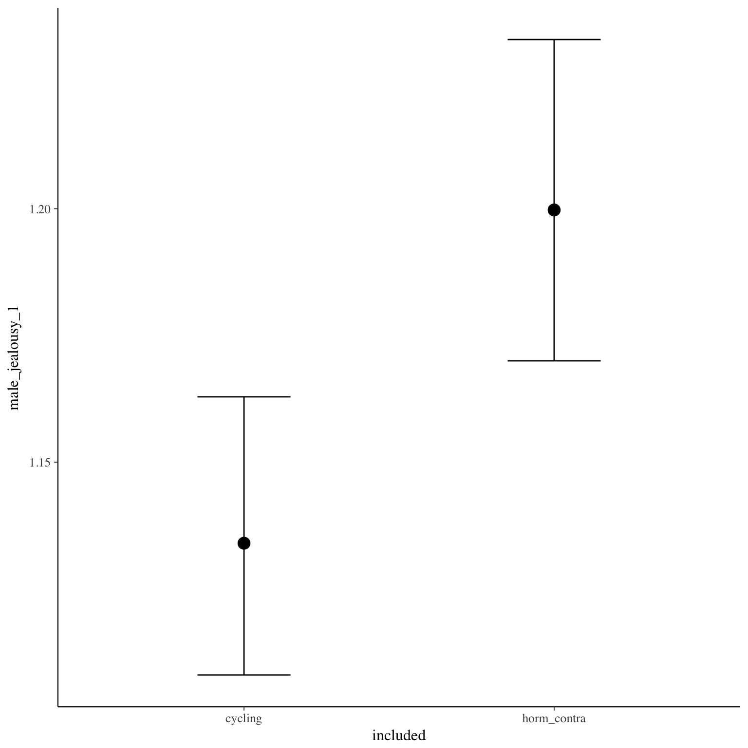
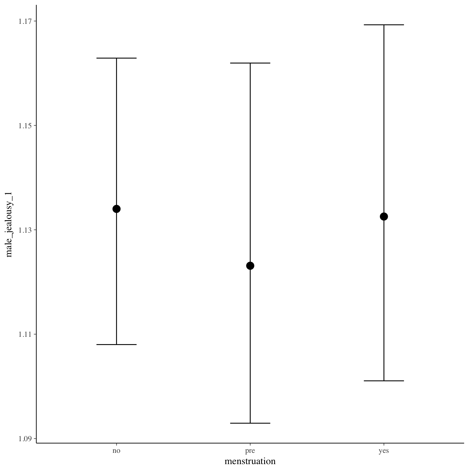
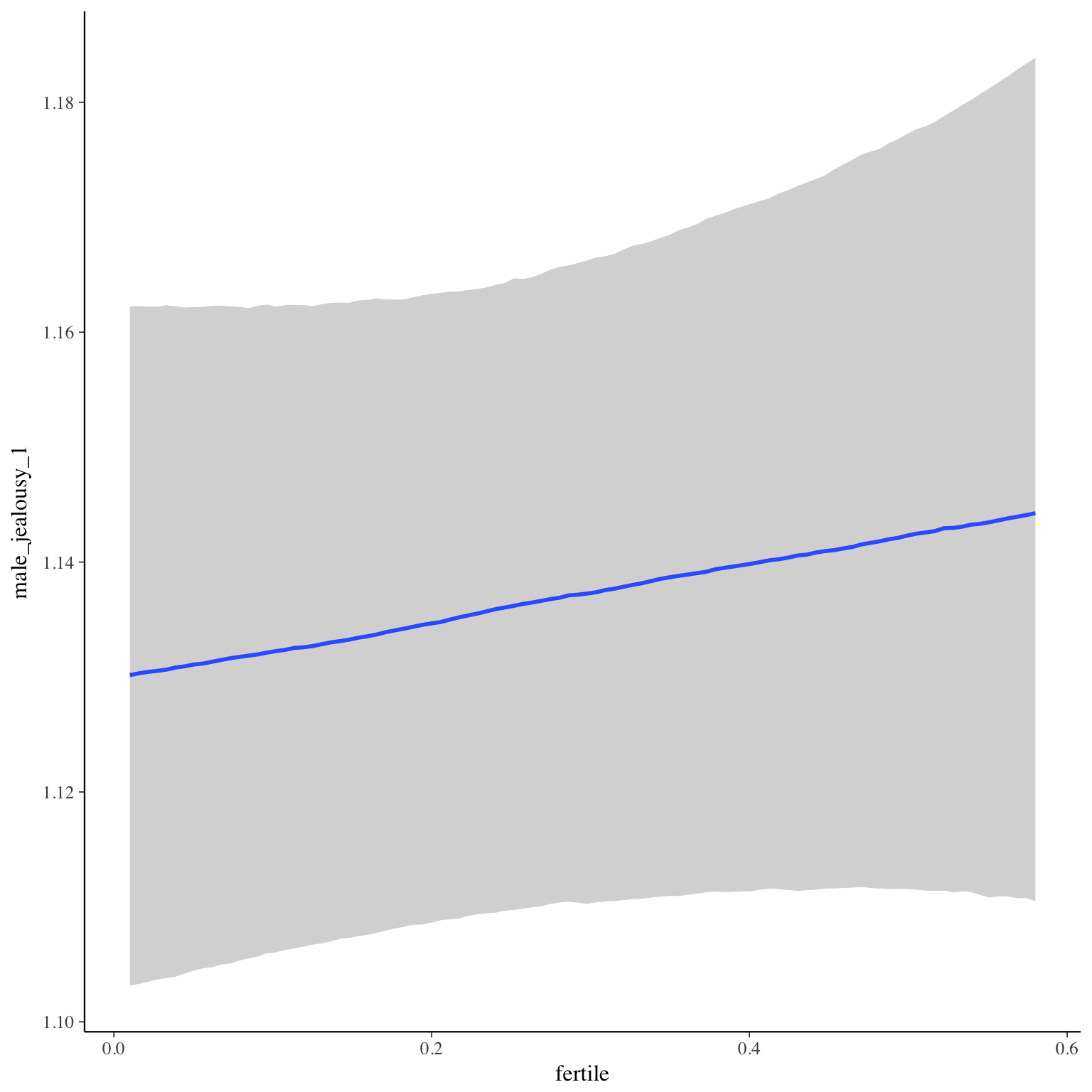
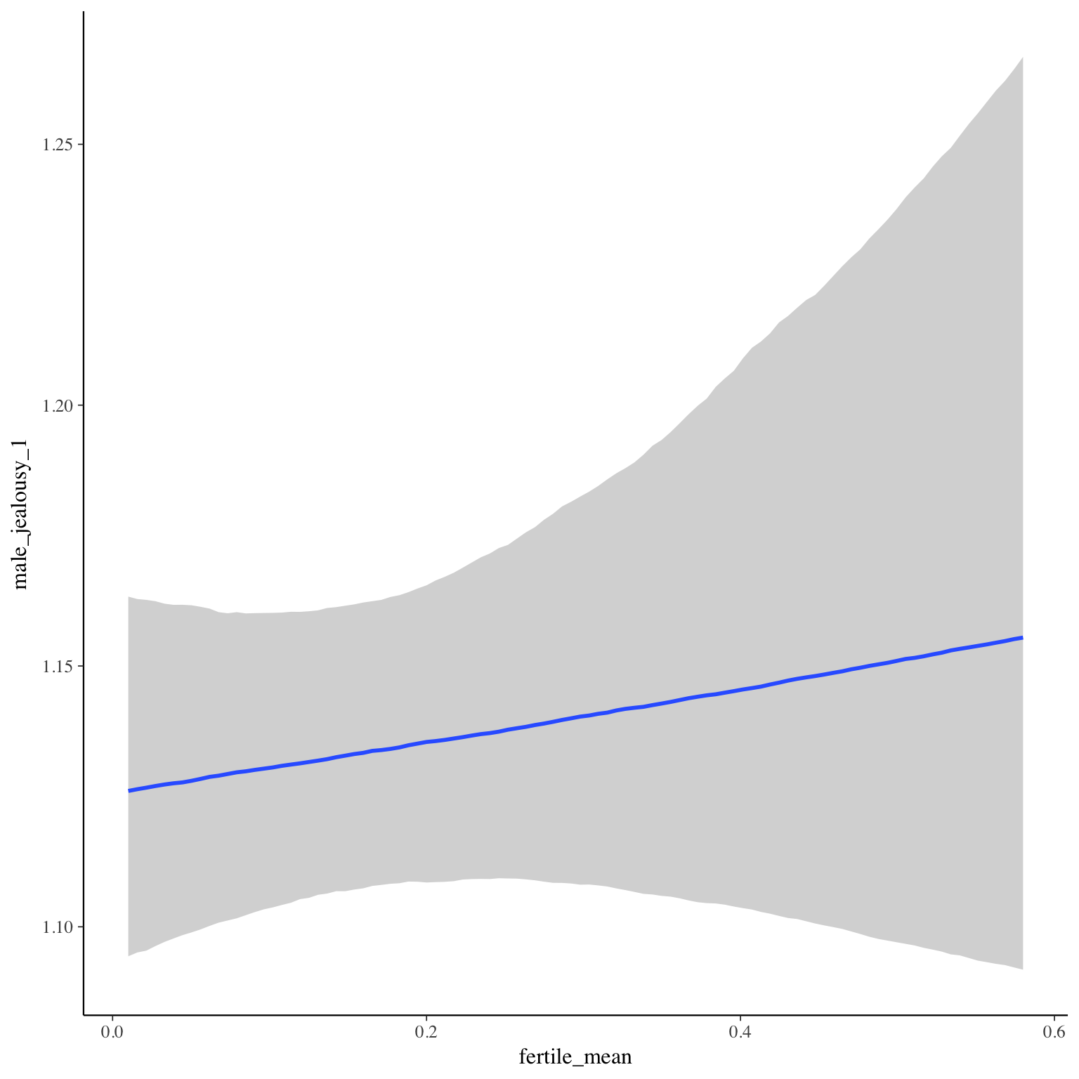
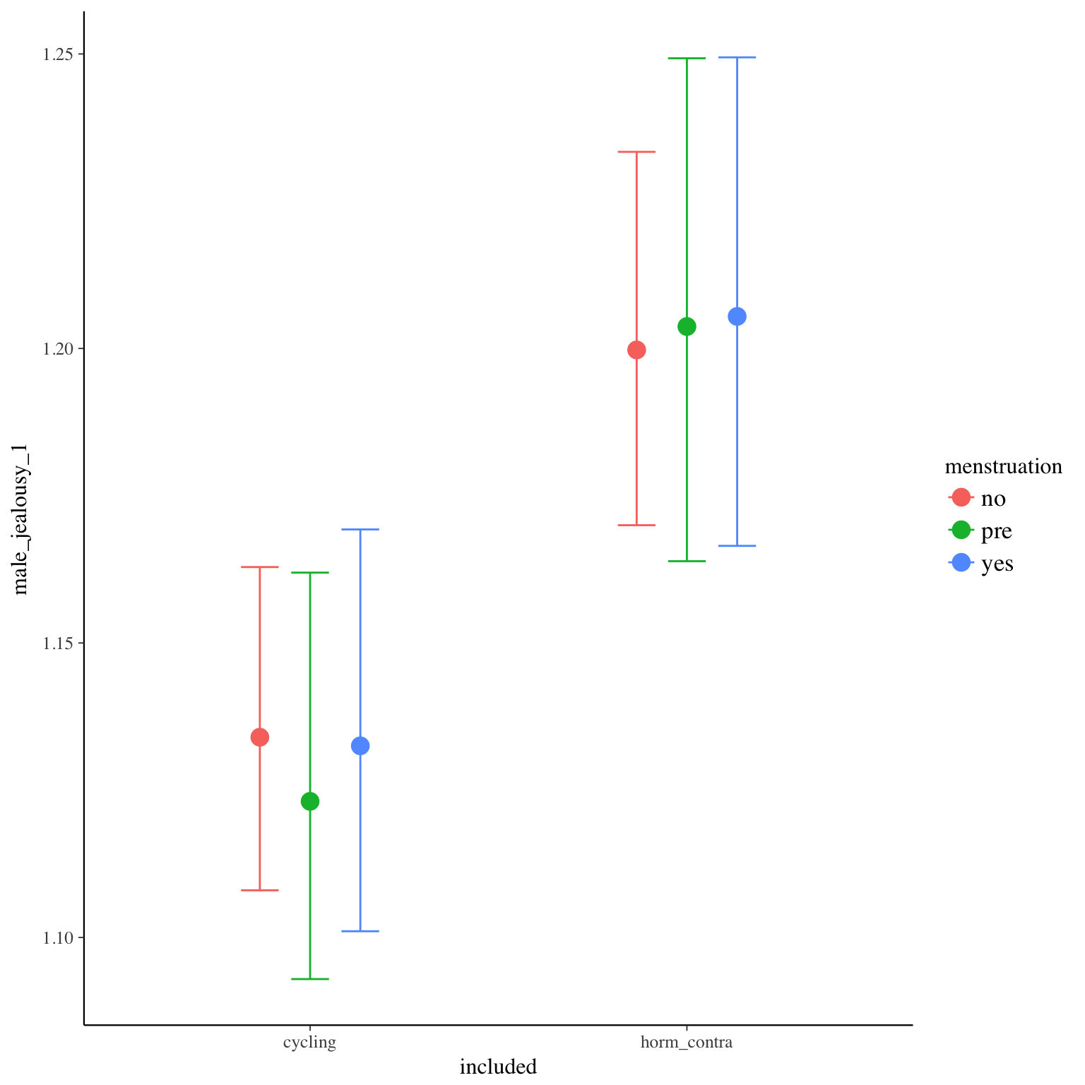
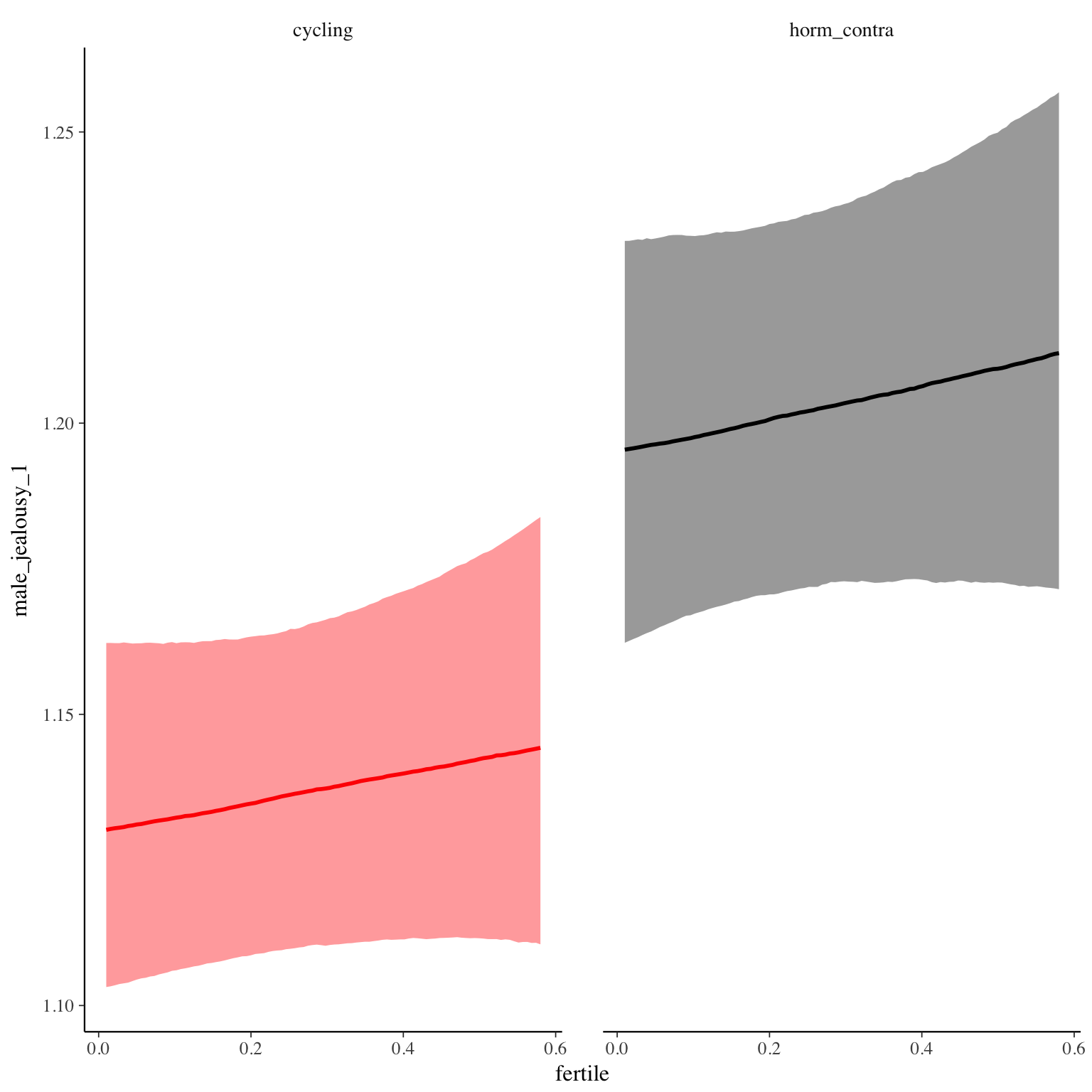
Diagnostics
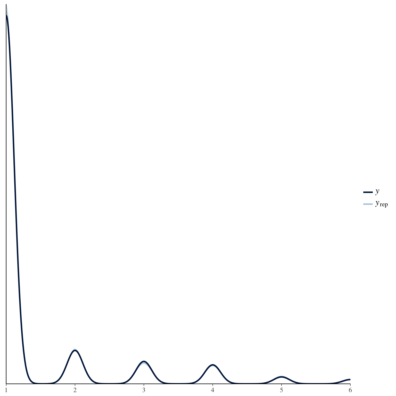
male_jealousy_2
Item text:
… hat mein Partner auf meinen Umgang mit anderen Männern eifersüchtig reagiert.
Item translation:
35. My partner was jealous of my contact with other men.
Choices:
| choice | value | frequency | percent |
|---|---|---|---|
| 1 | Stimme nicht zu | 24805 | 0.83 |
| 2 | Stimme überwiegend nicht zu | 1817 | 0.06 |
| 3 | Stimme eher nicht zu | 1312 | 0.04 |
| 4 | Stimme eher zu | 1176 | 0.04 |
| 5 | Stimme überwiegend zu | 433 | 0.01 |
| 6 | Stimme voll zu | 334 | 0.01 |
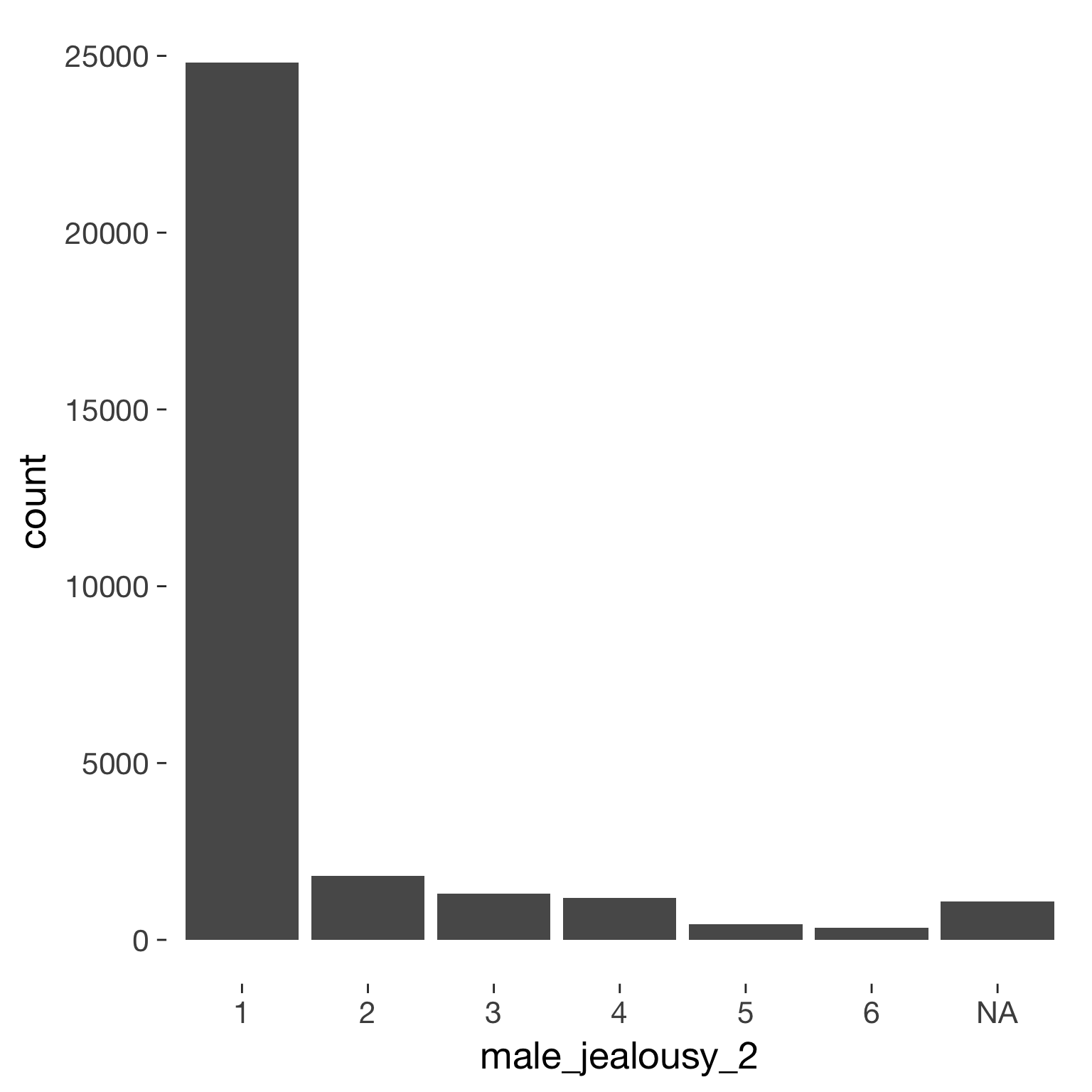
Model
Model summary
 Family: cumulative(logit)
Formula: male_jealousy_2 ~ included * (menstruation + fertile) + fertile_mean + (1 + fertile + menstruation | person)
         disc = 1
   Data: diary (Number of observations: 26546)
Samples: 4 chains, each with iter = 2000; warmup = 1000; thin = 1;
         total post-warmup samples = 4000
    ICs: LOO = 30431.82; WAIC = Not computed

Group-Level Effects:
~person (Number of levels: 1043)
                                     Estimate Est.Error l-95% CI u-95% CI Eff.Sample Rhat
sd(Intercept)                            1.99      0.08     1.84     2.17        738 1.00
sd(fertile)                              1.65      0.21     1.23     2.05        449 1.01
sd(menstruationpre)                      0.57      0.14     0.26     0.81        262 1.02
sd(menstruationyes)                      0.72      0.12     0.47     0.94        456 1.01
cor(Intercept,fertile)                  -0.17      0.11    -0.38     0.05       1551 1.00
cor(Intercept,menstruationpre)          -0.03      0.17    -0.34     0.32       1477 1.00
cor(fertile,menstruationpre)             0.28      0.21    -0.18     0.63        314 1.01
cor(Intercept,menstruationyes)           0.12      0.13    -0.15     0.39       1171 1.00
cor(fertile,menstruationyes)             0.46      0.15     0.11     0.72        439 1.01
cor(menstruationpre,menstruationyes)     0.77      0.14     0.46     0.96        451 1.00

Population-Level Effects:
                                    Estimate Est.Error l-95% CI u-95% CI Eff.Sample Rhat
Intercept[1]                            2.46      0.18     2.11     2.82        836    1
Intercept[2]                            3.21      0.19     2.85     3.57        840    1
Intercept[3]                            3.95      0.19     3.59     4.33        845    1
Intercept[4]                            5.12      0.19     4.75     5.50        855    1
Intercept[5]                            6.07      0.19     5.69     6.45        889    1
includedhorm_contra                    -0.08      0.16    -0.40     0.23        686    1
menstruationpre                        -0.24      0.12    -0.47     0.01       1593    1
menstruationyes                        -0.49      0.13    -0.74    -0.23       1748    1
fertile                                 0.11      0.25    -0.37     0.58       1979    1
fertile_mean                            0.65      0.72    -0.64     2.14       1613    1
includedhorm_contra:menstruationpre     0.20      0.13    -0.06     0.47       2124    1
includedhorm_contra:menstruationyes     0.34      0.14     0.07     0.61       2381    1
includedhorm_contra:fertile            -0.11      0.27    -0.65     0.41       2138    1

Samples were drawn using sampling(NUTS). For each parameter, Eff.Sample
is a crude measure of effective sample size, and Rhat is the potential
scale reduction factor on split chains (at convergence, Rhat = 1).
Coefficient plot
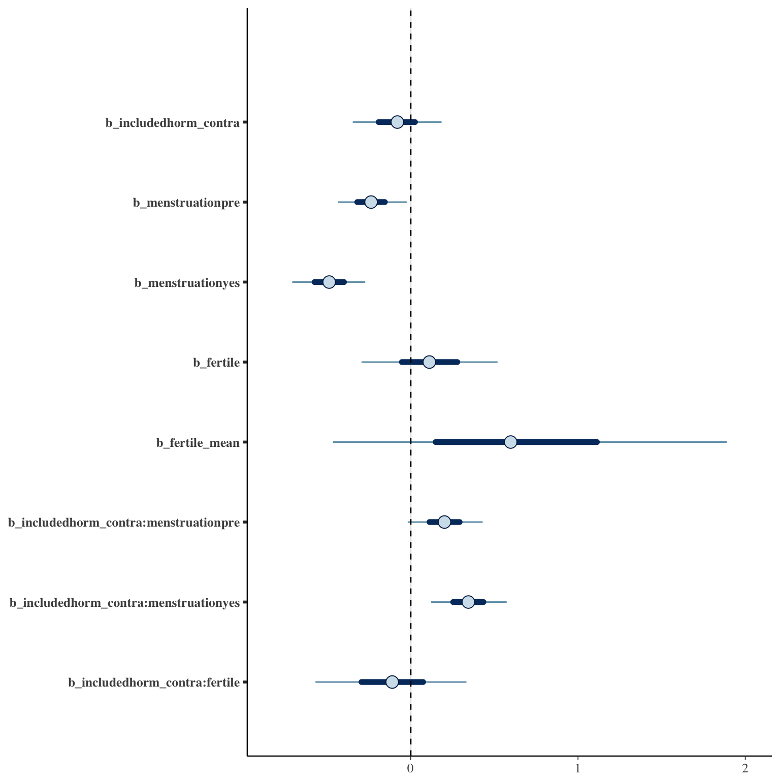
Marginal effect plots
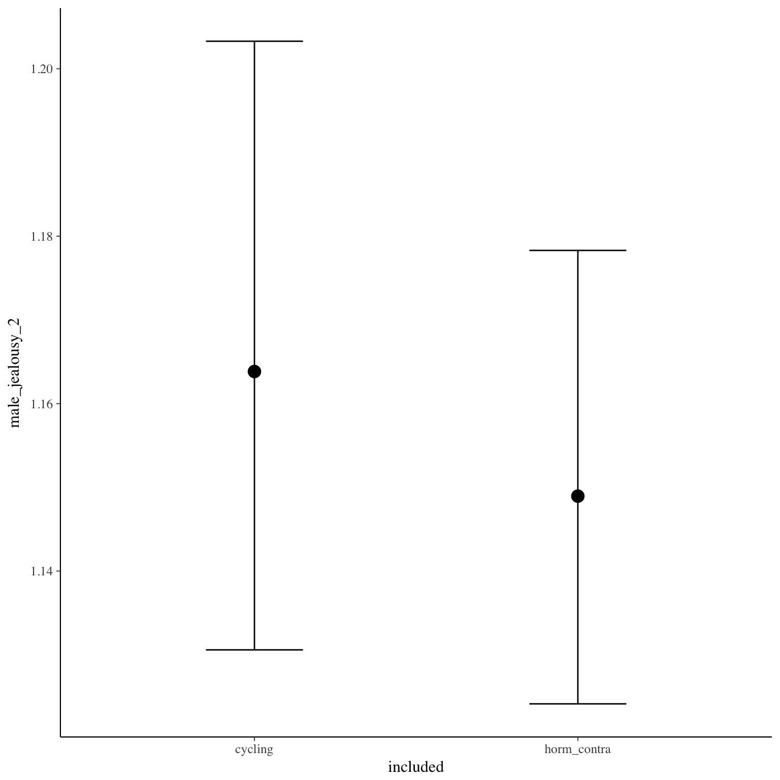
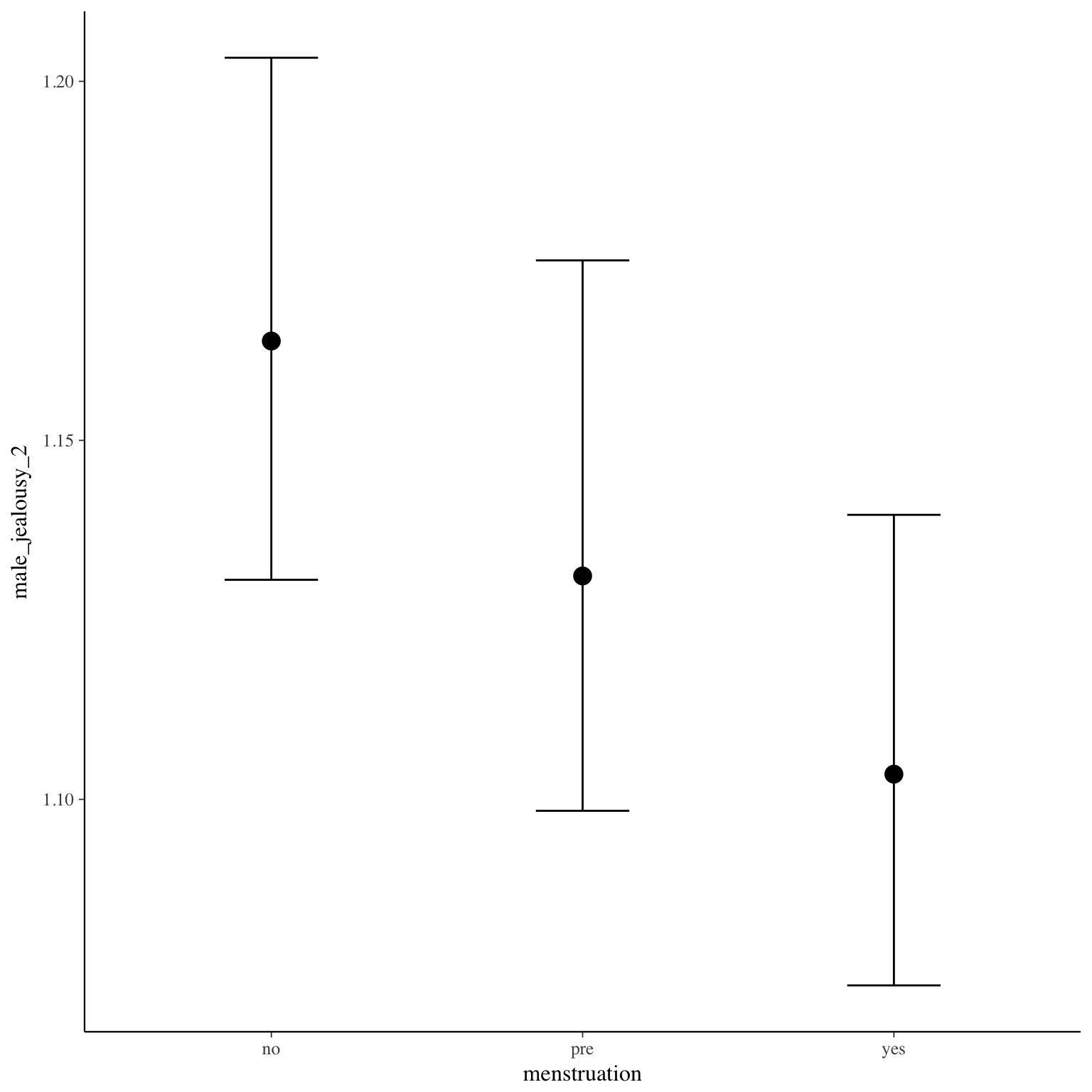
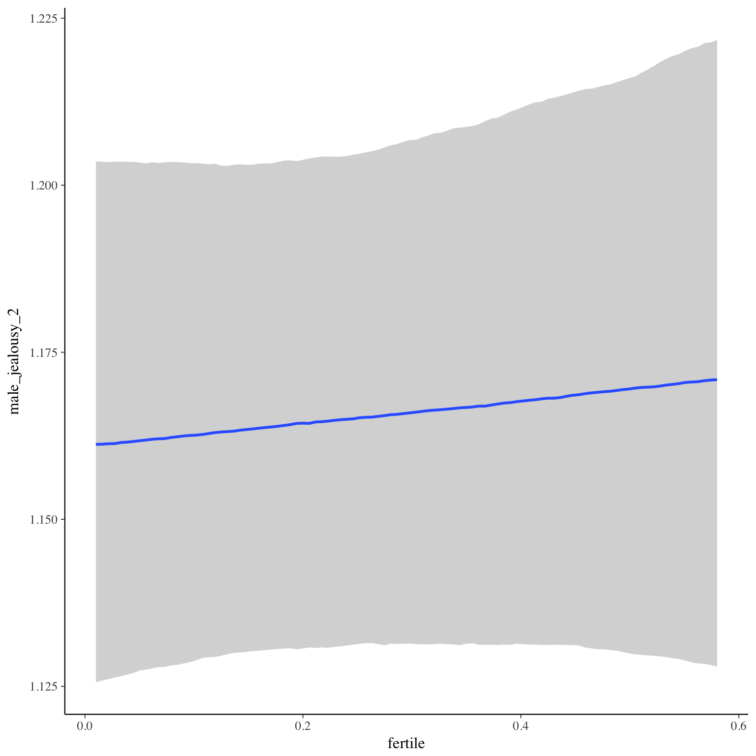
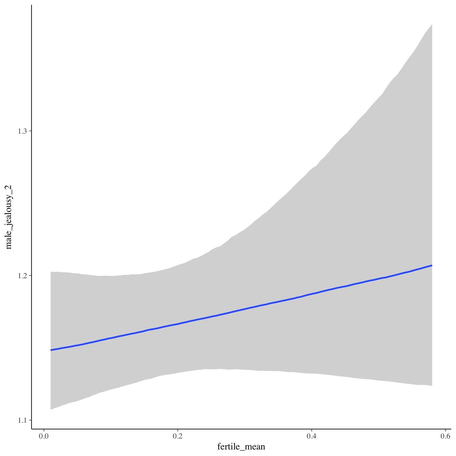
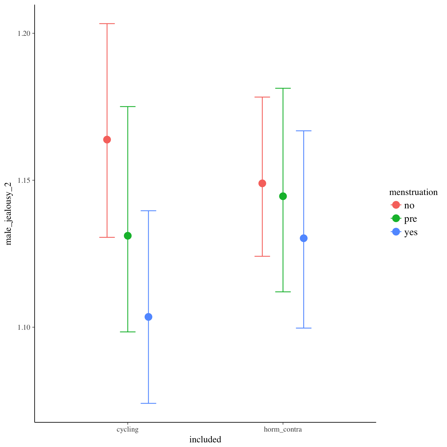
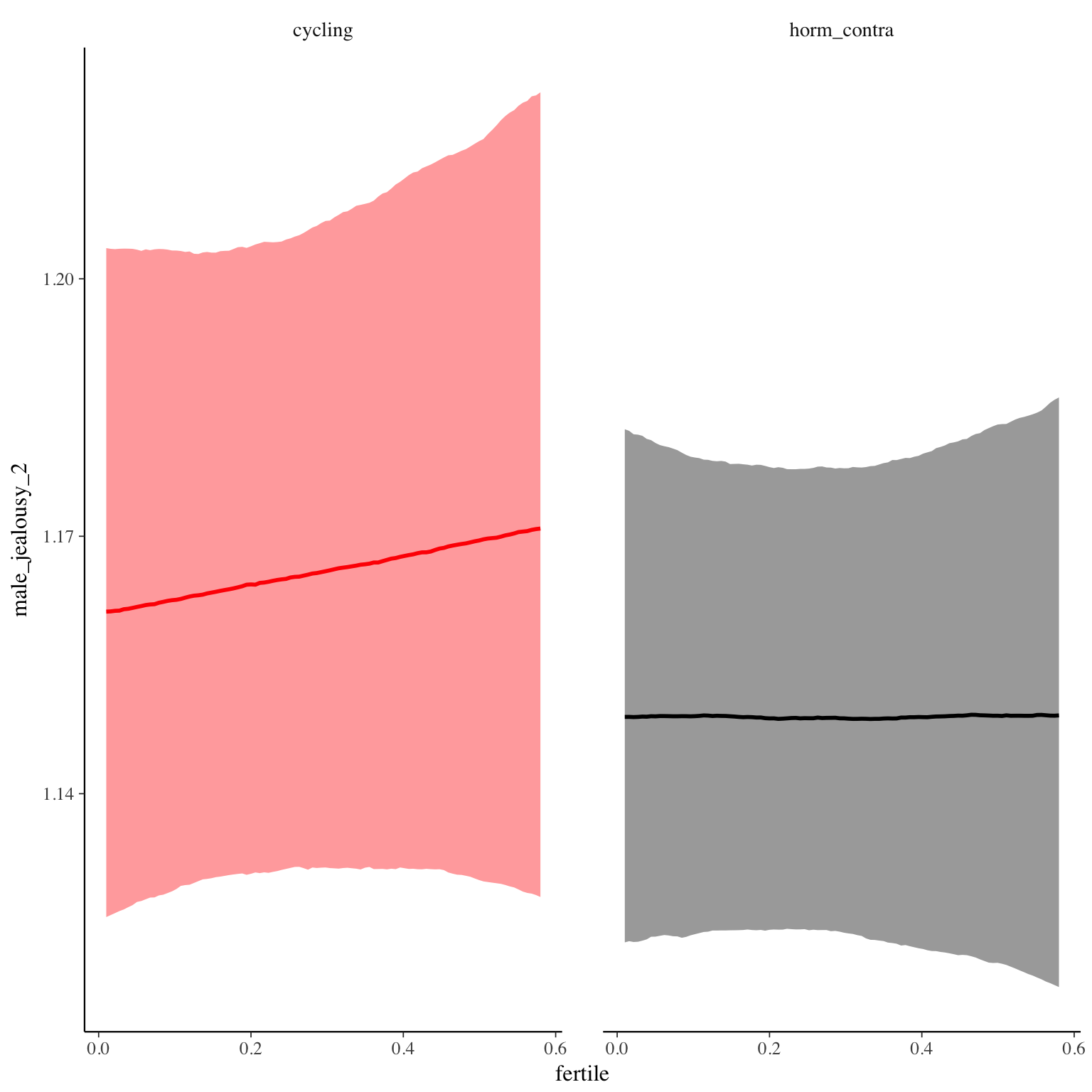
Diagnostics
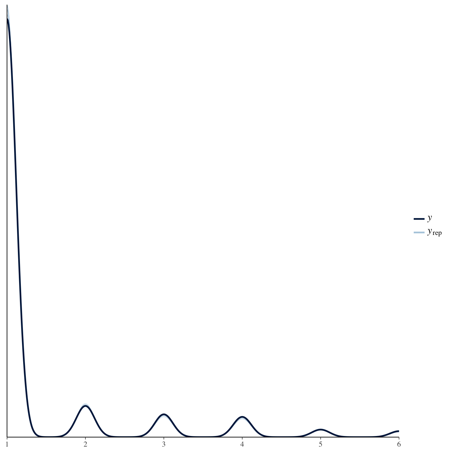
male_jealousy_3
Item text:
… hat mir mein Partner erzählt, er habe Komplimente von anderen Frauen erhalten.
Item translation:
36. My partner told me he had received compliments from other women.
Choices:
| choice | value | frequency | percent |
|---|---|---|---|
| 1 | Stimme nicht zu | 27378 | 0.92 |
| 2 | Stimme überwiegend nicht zu | 1128 | 0.04 |
| 3 | Stimme eher nicht zu | 600 | 0.02 |
| 4 | Stimme eher zu | 403 | 0.01 |
| 5 | Stimme überwiegend zu | 191 | 0.01 |
| 6 | Stimme voll zu | 176 | 0.01 |
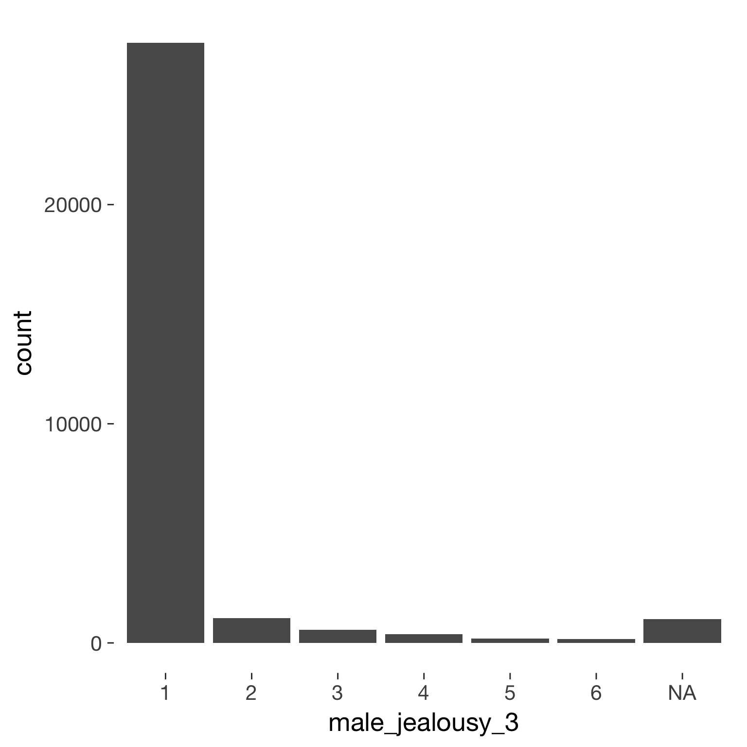
Model
Model summary
 Family: cumulative(logit)
Formula: male_jealousy_3 ~ included * (menstruation + fertile) + fertile_mean + (1 + fertile + menstruation | person)
         disc = 1
   Data: diary (Number of observations: 26545)
Samples: 4 chains, each with iter = 2000; warmup = 1000; thin = 1;
         total post-warmup samples = 4000
    ICs: LOO = 16673.68; WAIC = Not computed

Group-Level Effects:
~person (Number of levels: 1043)
                                     Estimate Est.Error l-95% CI u-95% CI Eff.Sample Rhat
sd(Intercept)                            2.05      0.09     1.87     2.22       1126 1.00
sd(fertile)                              0.63      0.34     0.05     1.31        302 1.02
sd(menstruationpre)                      0.41      0.22     0.03     0.84        465 1.01
sd(menstruationyes)                      0.16      0.12     0.01     0.44        824 1.00
cor(Intercept,fertile)                   0.28      0.29    -0.36     0.82       3245 1.00
cor(Intercept,menstruationpre)           0.11      0.28    -0.46     0.68       4000 1.00
cor(fertile,menstruationpre)             0.17      0.41    -0.68     0.82        435 1.01
cor(Intercept,menstruationyes)          -0.04      0.40    -0.78     0.73       4000 1.00
cor(fertile,menstruationyes)             0.00      0.45    -0.81     0.80       2353 1.00
cor(menstruationpre,menstruationyes)    -0.09      0.44    -0.85     0.75       2769 1.00

Population-Level Effects:
                                    Estimate Est.Error l-95% CI u-95% CI Eff.Sample Rhat
Intercept[1]                            3.66      0.21     3.24     4.07       1992    1
Intercept[2]                            4.55      0.21     4.13     4.97       1998    1
Intercept[3]                            5.28      0.21     4.86     5.69       2024    1
Intercept[4]                            6.12      0.21     5.69     6.54       1774    1
Intercept[5]                            6.92      0.22     6.47     7.35       1758    1
includedhorm_contra                    -0.05      0.18    -0.40     0.30       1613    1
menstruationpre                        -0.12      0.18    -0.50     0.22       2054    1
menstruationyes                        -0.02      0.14    -0.30     0.26       4000    1
fertile                                -0.32      0.33    -1.01     0.28       1821    1
fertile_mean                           -0.44      0.82    -2.19     1.07       2427    1
includedhorm_contra:menstruationpre     0.07      0.16    -0.25     0.38       4000    1
includedhorm_contra:menstruationyes     0.14      0.15    -0.16     0.43       4000    1
includedhorm_contra:fertile            -0.26      0.30    -0.86     0.32       4000    1

Samples were drawn using sampling(NUTS). For each parameter, Eff.Sample
is a crude measure of effective sample size, and Rhat is the potential
scale reduction factor on split chains (at convergence, Rhat = 1).
Coefficient plot
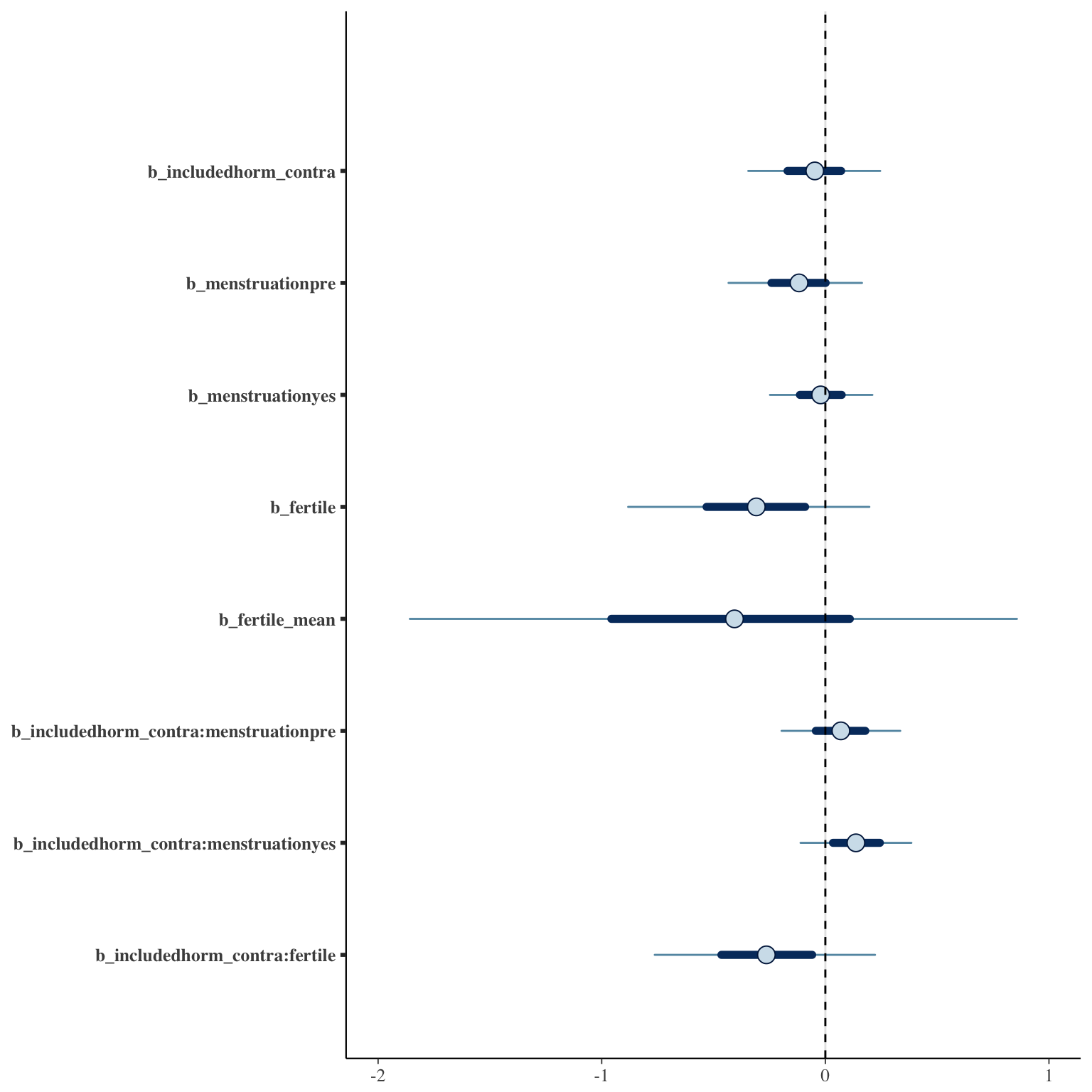
Marginal effect plots
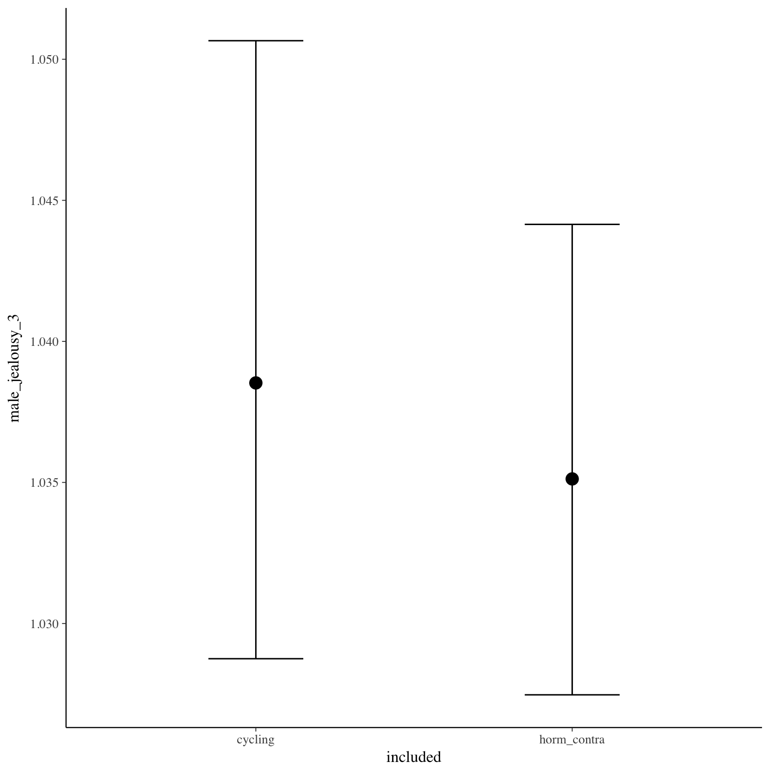
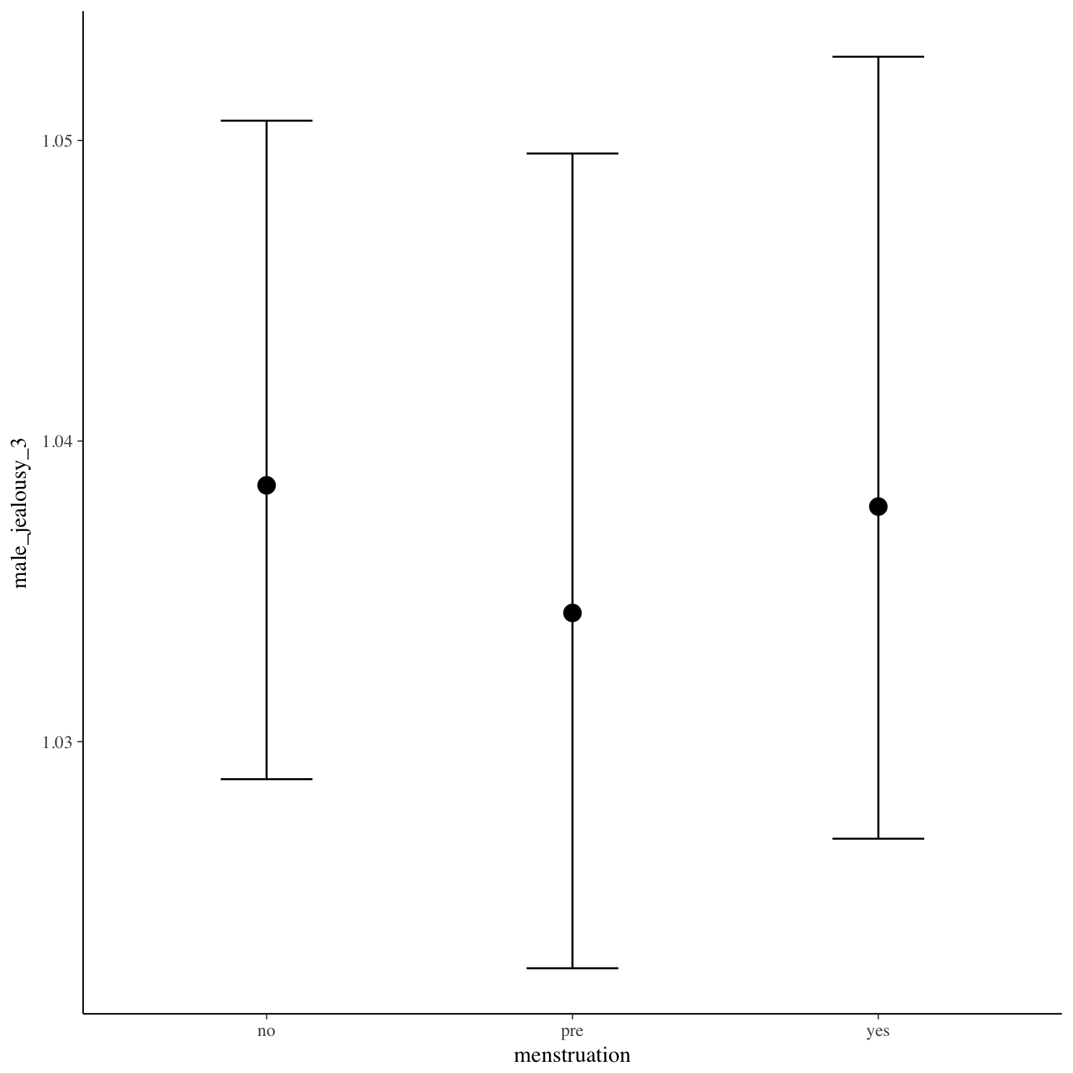
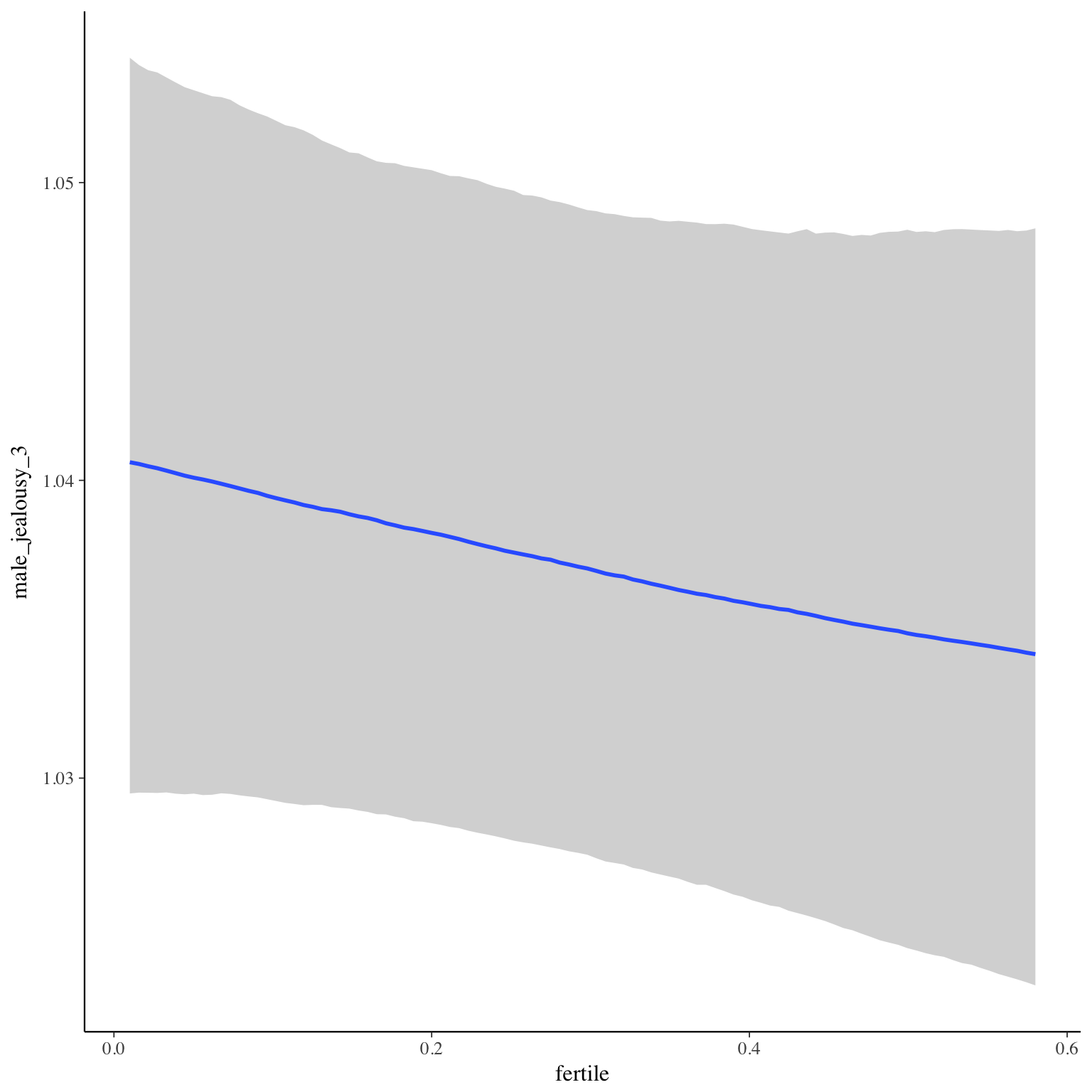
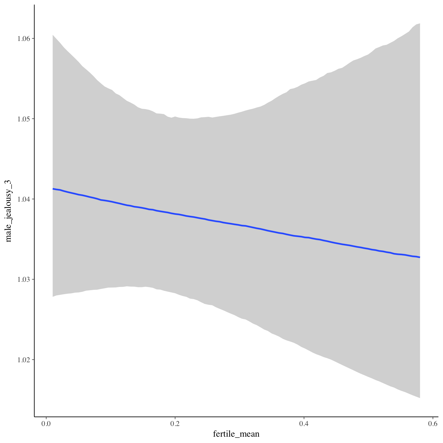
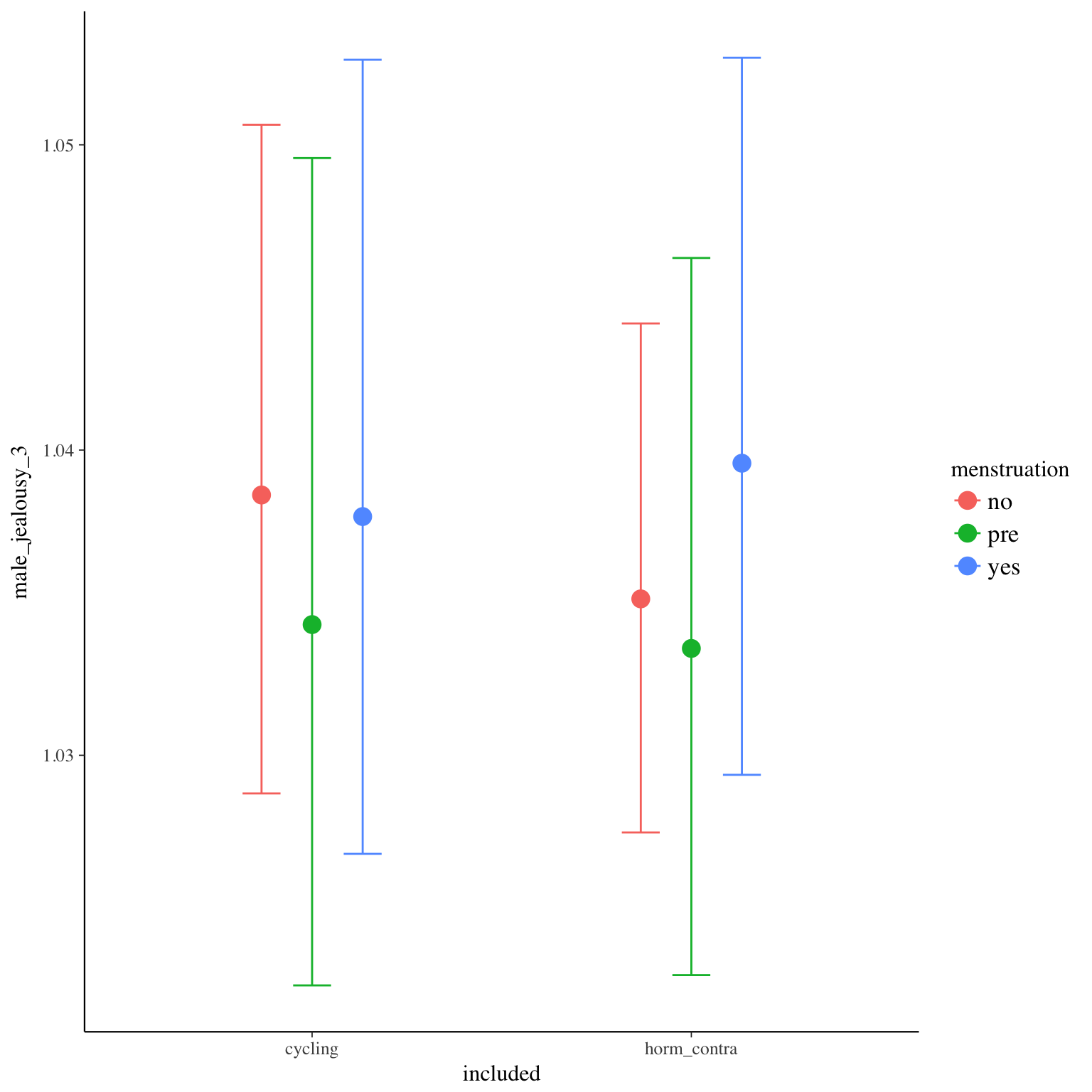
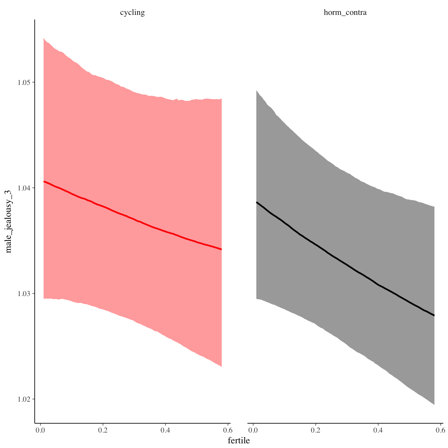
Diagnostics

male_mate_retention_1
Item text:
… hat mich mein Partner gefragt, mit wem ich den Tag verbracht habe.
Item translation:
43. My partner asked me with whom I spent the day.
Choices:
| choice | value | frequency | percent |
|---|---|---|---|
| 1 | Stimme nicht zu | 17532 | 0.59 |
| 2 | Stimme überwiegend nicht zu | 1787 | 0.06 |
| 3 | Stimme eher nicht zu | 2043 | 0.07 |
| 4 | Stimme eher zu | 3564 | 0.12 |
| 5 | Stimme überwiegend zu | 2062 | 0.07 |
| 6 | Stimme voll zu | 2888 | 0.1 |
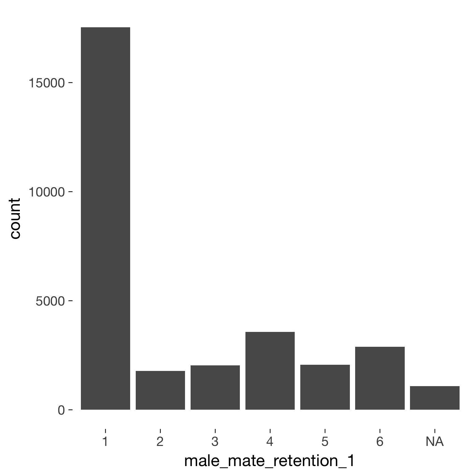
Model
Model summary
 Family: cumulative(logit)
Formula: male_mate_retention_1 ~ included * (menstruation + fertile) + fertile_mean + (1 + fertile + menstruation | person)
         disc = 1
   Data: diary (Number of observations: 26545)
Samples: 4 chains, each with iter = 2000; warmup = 1000; thin = 1;
         total post-warmup samples = 4000
    ICs: LOO = 56670.01; WAIC = Not computed

Group-Level Effects:
~person (Number of levels: 1043)
                                     Estimate Est.Error l-95% CI u-95% CI Eff.Sample Rhat
sd(Intercept)                            2.18      0.07     2.04     2.33        570 1.00
sd(fertile)                              1.68      0.15     1.36     1.97        635 1.00
sd(menstruationpre)                      0.66      0.08     0.48     0.82        343 1.01
sd(menstruationyes)                      0.71      0.08     0.55     0.85        680 1.00
cor(Intercept,fertile)                  -0.08      0.09    -0.25     0.10       2077 1.00
cor(Intercept,menstruationpre)           0.01      0.11    -0.20     0.24       1698 1.00
cor(fertile,menstruationpre)             0.16      0.15    -0.17     0.40        306 1.01
cor(Intercept,menstruationyes)          -0.15      0.10    -0.35     0.05       2010 1.00
cor(fertile,menstruationyes)             0.39      0.12     0.13     0.60        481 1.00
cor(menstruationpre,menstruationyes)     0.52      0.13     0.26     0.76        380 1.01

Population-Level Effects:
                                    Estimate Est.Error l-95% CI u-95% CI Eff.Sample Rhat
Intercept[1]                            0.58      0.17     0.24     0.91        489 1.01
Intercept[2]                            1.00      0.17     0.66     1.33        491 1.01
Intercept[3]                            1.52      0.17     1.18     1.84        493 1.01
Intercept[4]                            2.61      0.17     2.27     2.94        494 1.01
Intercept[5]                            3.54      0.17     3.19     3.87        503 1.01
includedhorm_contra                     0.08      0.15    -0.23     0.37        358 1.00
menstruationpre                        -0.12      0.09    -0.29     0.05       1813 1.00
menstruationyes                        -0.08      0.09    -0.25     0.08       1904 1.00
fertile                                -0.10      0.19    -0.47     0.26       1871 1.00
fertile_mean                           -0.32      0.69    -1.81     0.97        819 1.00
includedhorm_contra:menstruationpre     0.16      0.10    -0.05     0.36       2033 1.00
includedhorm_contra:menstruationyes     0.09      0.10    -0.11     0.30       1930 1.00
includedhorm_contra:fertile             0.20      0.22    -0.24     0.63       1780 1.00

Samples were drawn using sampling(NUTS). For each parameter, Eff.Sample
is a crude measure of effective sample size, and Rhat is the potential
scale reduction factor on split chains (at convergence, Rhat = 1).
Coefficient plot
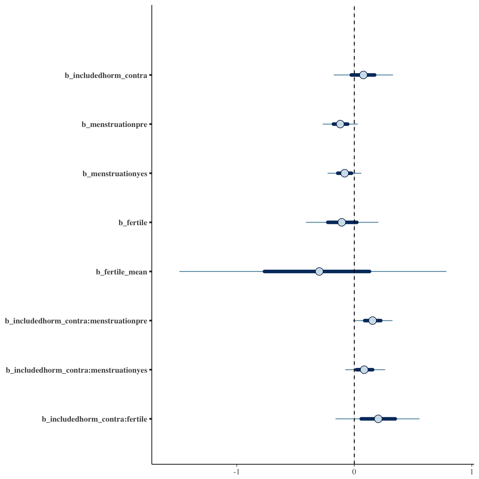
Marginal effect plots
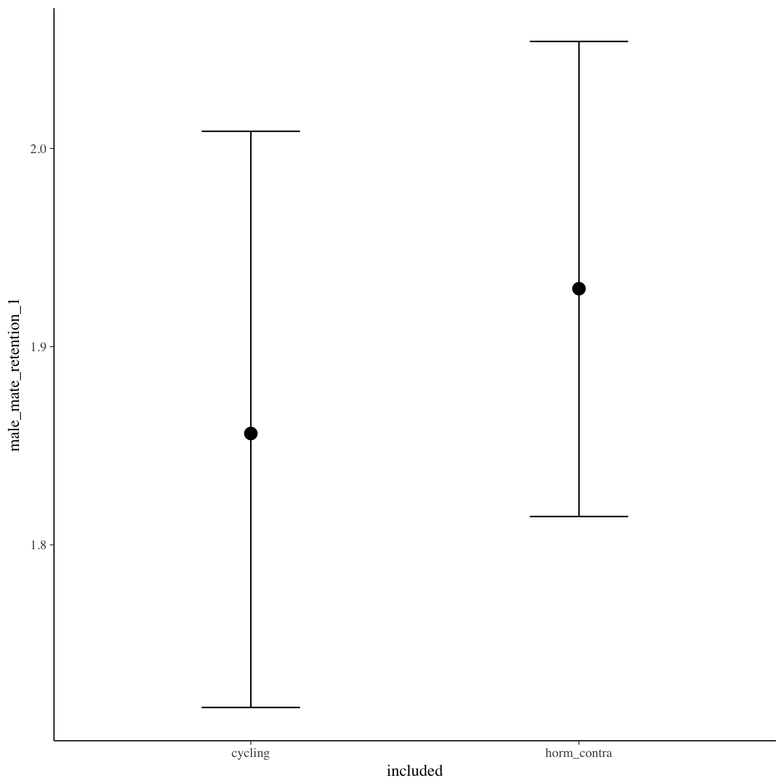
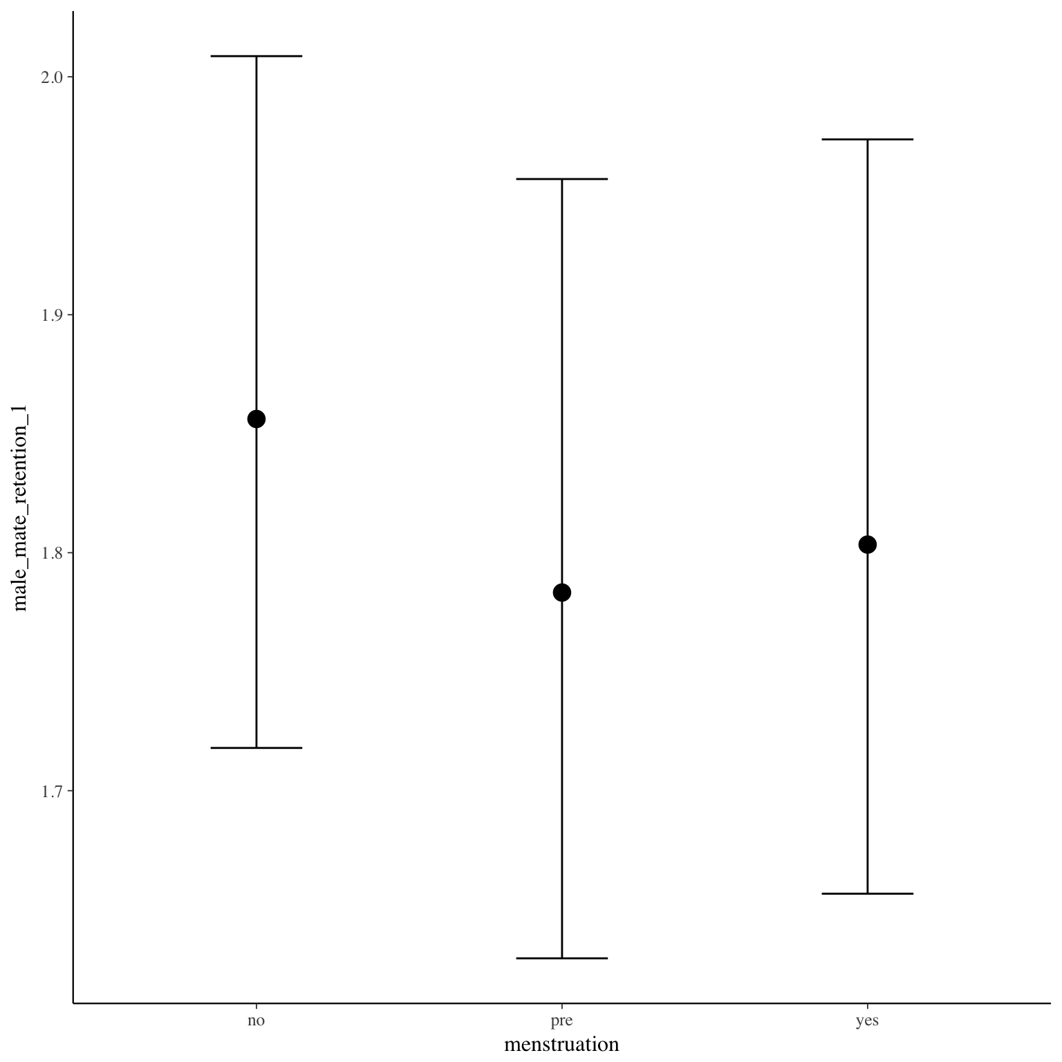
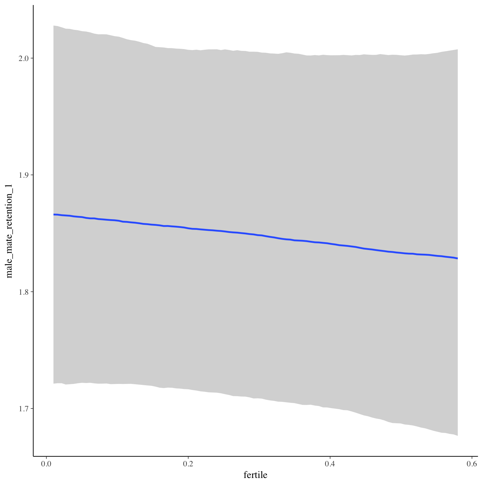
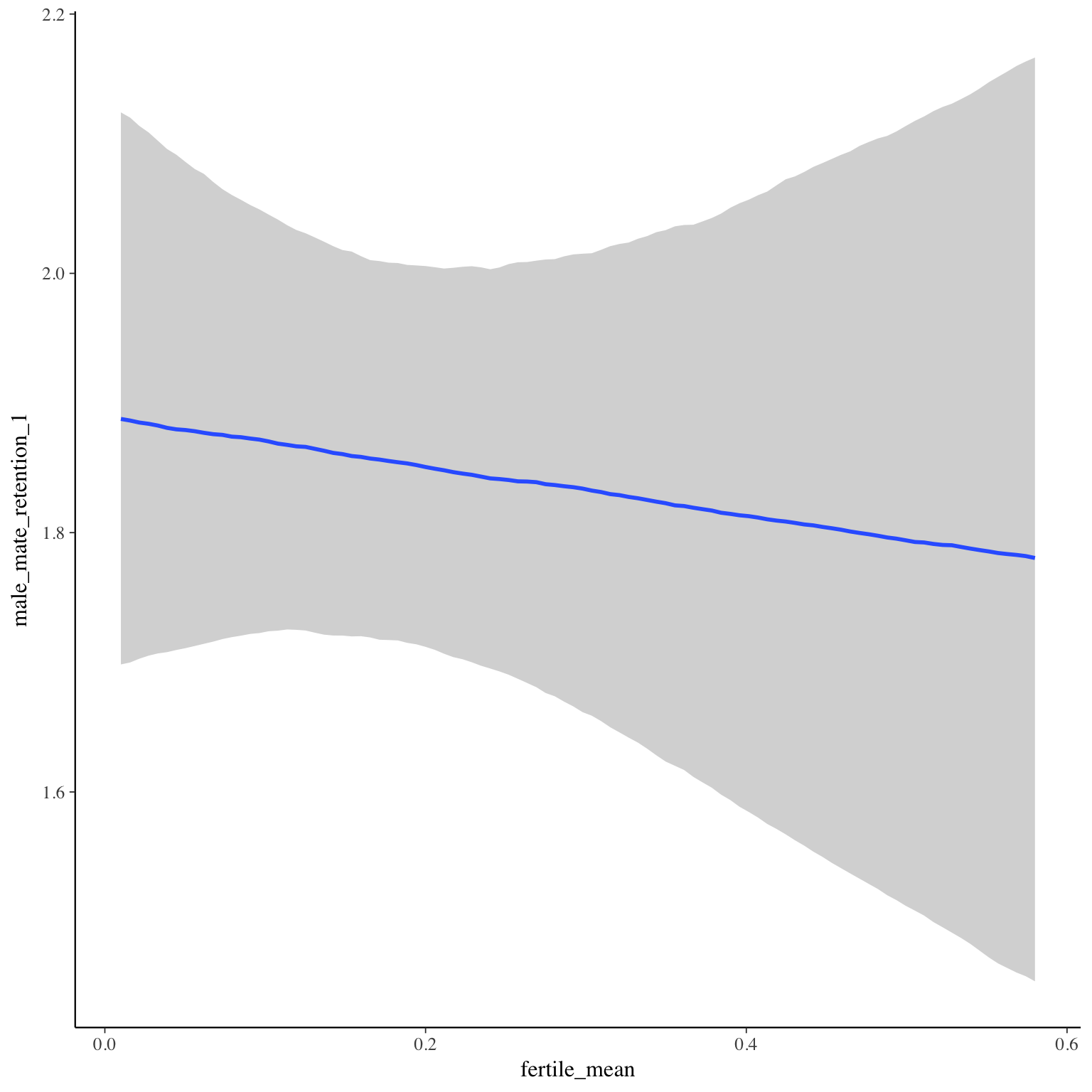
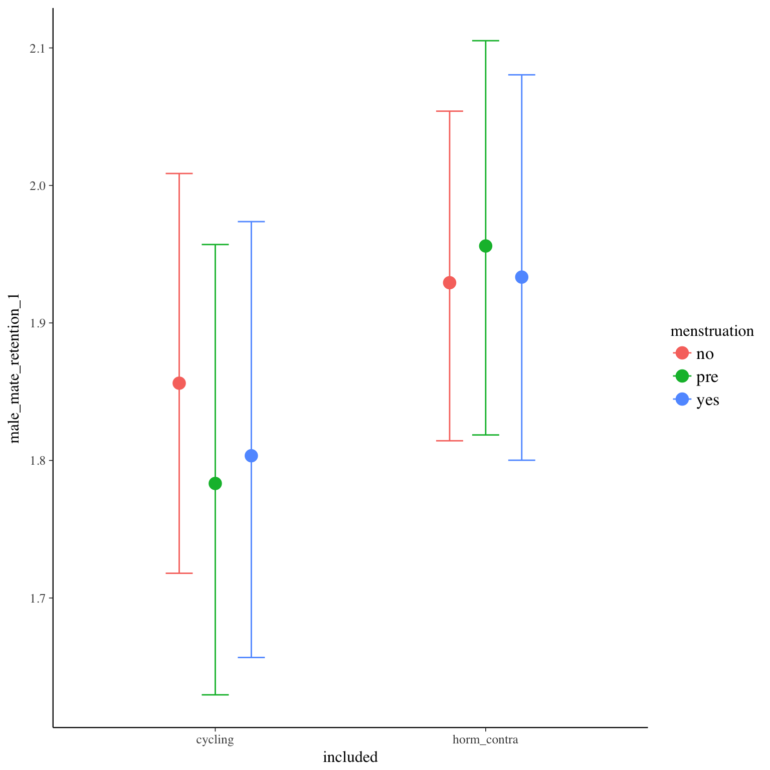
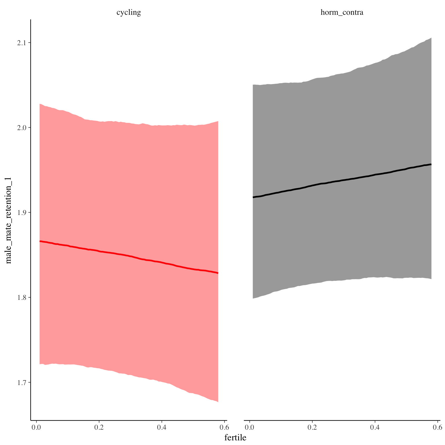
Diagnostics
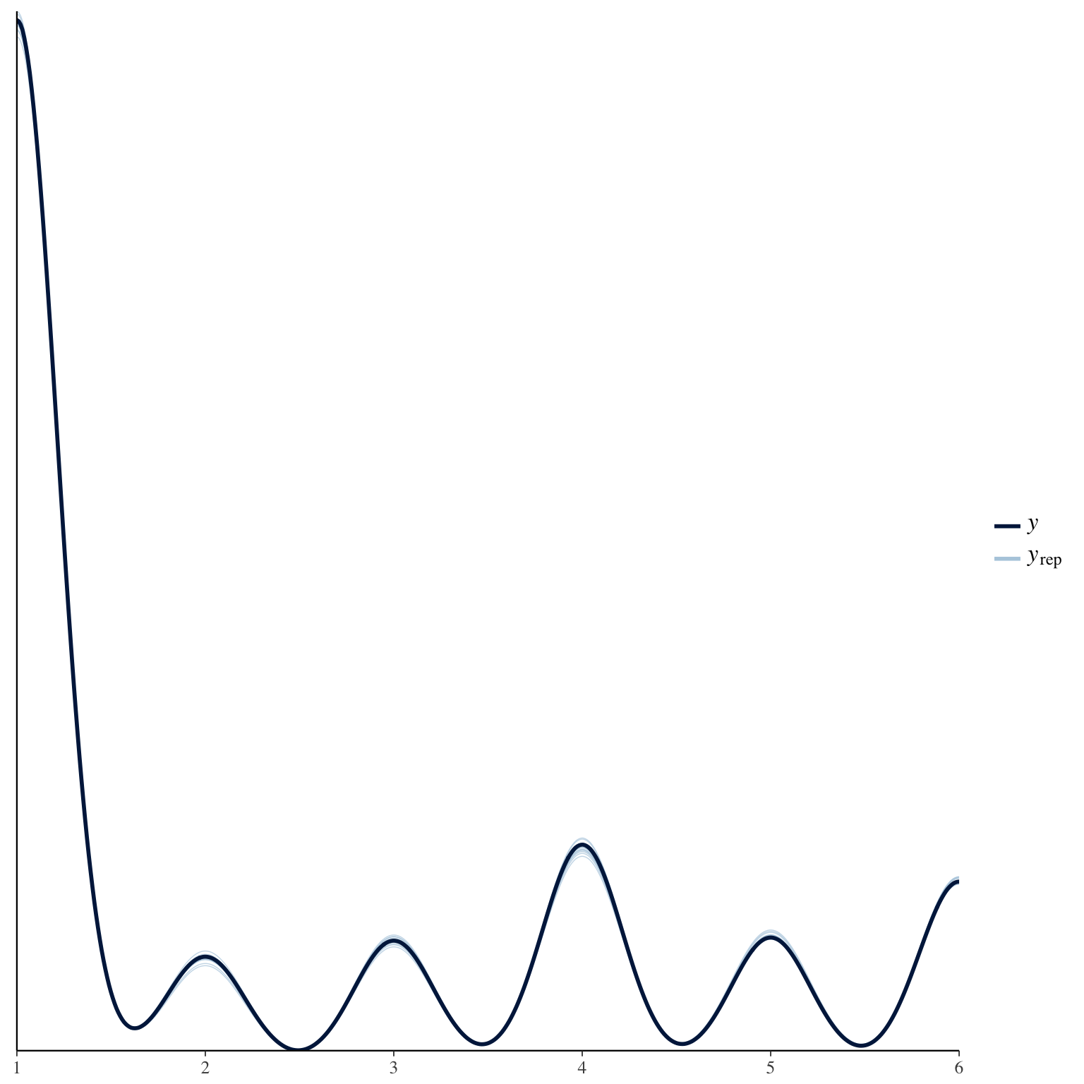
male_mate_retention_2
Item text:
… hat mir mein Partner gesagt, dass er mich liebt.
Item translation:
44. My partner told me he loved me.
Choices:
| choice | value | frequency | percent |
|---|---|---|---|
| 1 | Stimme nicht zu | 7590 | 0.25 |
| 2 | Stimme überwiegend nicht zu | 1225 | 0.04 |
| 3 | Stimme eher nicht zu | 2136 | 0.07 |
| 4 | Stimme eher zu | 3458 | 0.12 |
| 5 | Stimme überwiegend zu | 3508 | 0.12 |
| 6 | Stimme voll zu | 11959 | 0.4 |
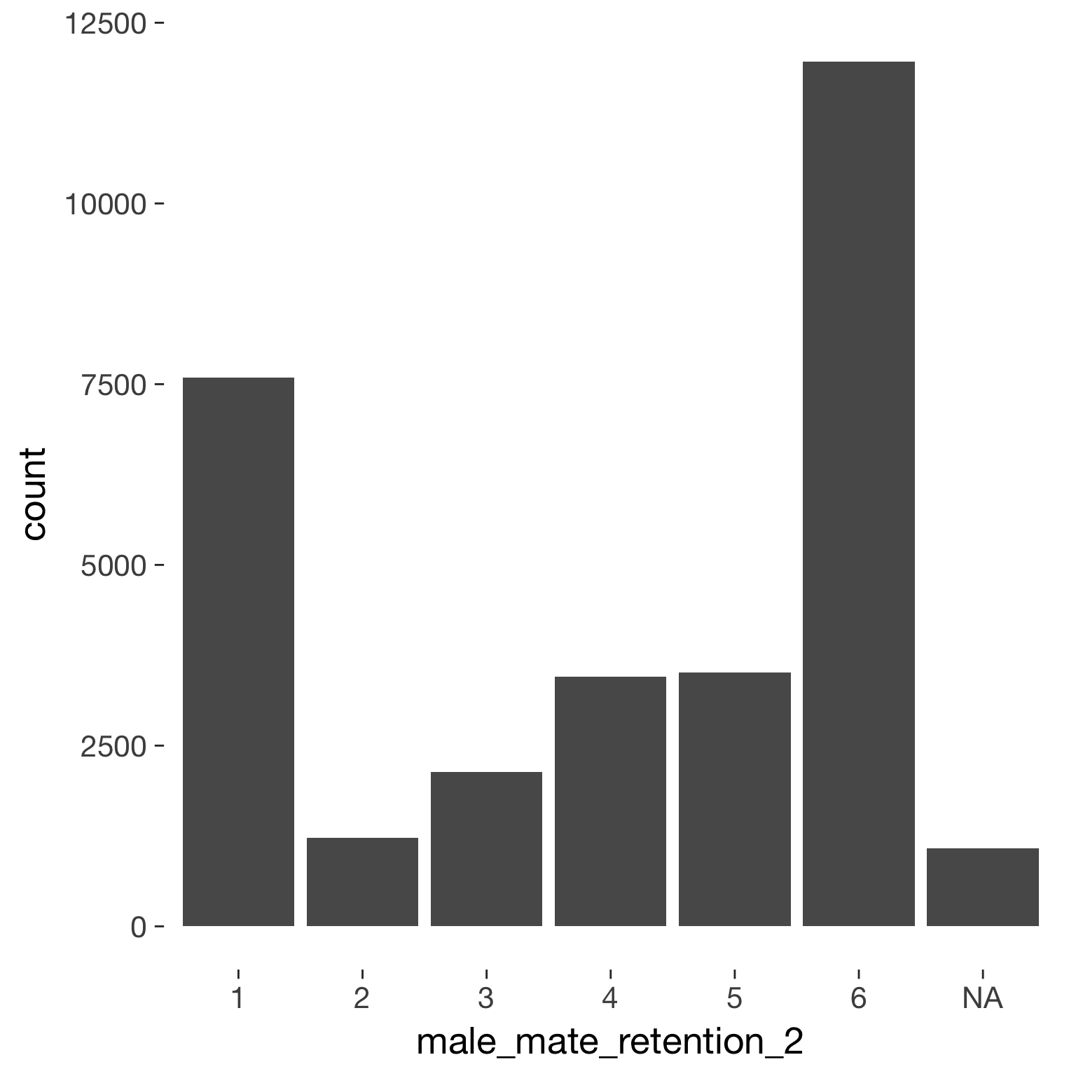
Model
Model summary
 Family: cumulative(logit)
Formula: male_mate_retention_2 ~ included * (menstruation + fertile) + fertile_mean + (1 + fertile + menstruation | person)
         disc = 1
   Data: diary (Number of observations: 26545)
Samples: 4 chains, each with iter = 2000; warmup = 1000; thin = 1;
         total post-warmup samples = 4000
    ICs: LOO = 61332.65; WAIC = Not computed

Group-Level Effects:
~person (Number of levels: 1043)
                                     Estimate Est.Error l-95% CI u-95% CI Eff.Sample Rhat
sd(Intercept)                            2.66      0.08     2.50     2.82        608 1.00
sd(fertile)                              1.21      0.16     0.90     1.52        301 1.01
sd(menstruationpre)                      0.57      0.09     0.37     0.73        347 1.01
sd(menstruationyes)                      0.61      0.08     0.45     0.75        425 1.01
cor(Intercept,fertile)                   0.02      0.13    -0.22     0.26       2014 1.00
cor(Intercept,menstruationpre)           0.27      0.14     0.00     0.54        993 1.00
cor(fertile,menstruationpre)            -0.11      0.21    -0.57     0.26        186 1.01
cor(Intercept,menstruationyes)          -0.05      0.13    -0.30     0.19       2363 1.00
cor(fertile,menstruationyes)             0.37      0.15     0.03     0.64        170 1.01
cor(menstruationpre,menstruationyes)     0.43      0.16     0.08     0.71        311 1.00

Population-Level Effects:
                                    Estimate Est.Error l-95% CI u-95% CI Eff.Sample Rhat
Intercept[1]                           -1.84      0.20    -2.24    -1.46        140 1.02
Intercept[2]                           -1.46      0.20    -1.86    -1.09        139 1.02
Intercept[3]                           -0.86      0.20    -1.26    -0.49        139 1.02
Intercept[4]                            0.01      0.20    -0.38     0.39        138 1.02
Intercept[5]                            0.91      0.20     0.51     1.29        139 1.02
includedhorm_contra                     0.39      0.17     0.05     0.72        124 1.04
menstruationpre                         0.03      0.07    -0.11     0.18       1451 1.00
menstruationyes                         0.04      0.07    -0.11     0.18       1563 1.00
fertile                                 0.15      0.15    -0.14     0.44       2065 1.00
fertile_mean                           -0.43      0.80    -2.11     1.13        571 1.01
includedhorm_contra:menstruationpre    -0.03      0.10    -0.22     0.16       1529 1.00
includedhorm_contra:menstruationyes    -0.14      0.09    -0.32     0.05       1681 1.00
includedhorm_contra:fertile            -0.32      0.19    -0.69     0.05       1916 1.00

Samples were drawn using sampling(NUTS). For each parameter, Eff.Sample
is a crude measure of effective sample size, and Rhat is the potential
scale reduction factor on split chains (at convergence, Rhat = 1).
Coefficient plot
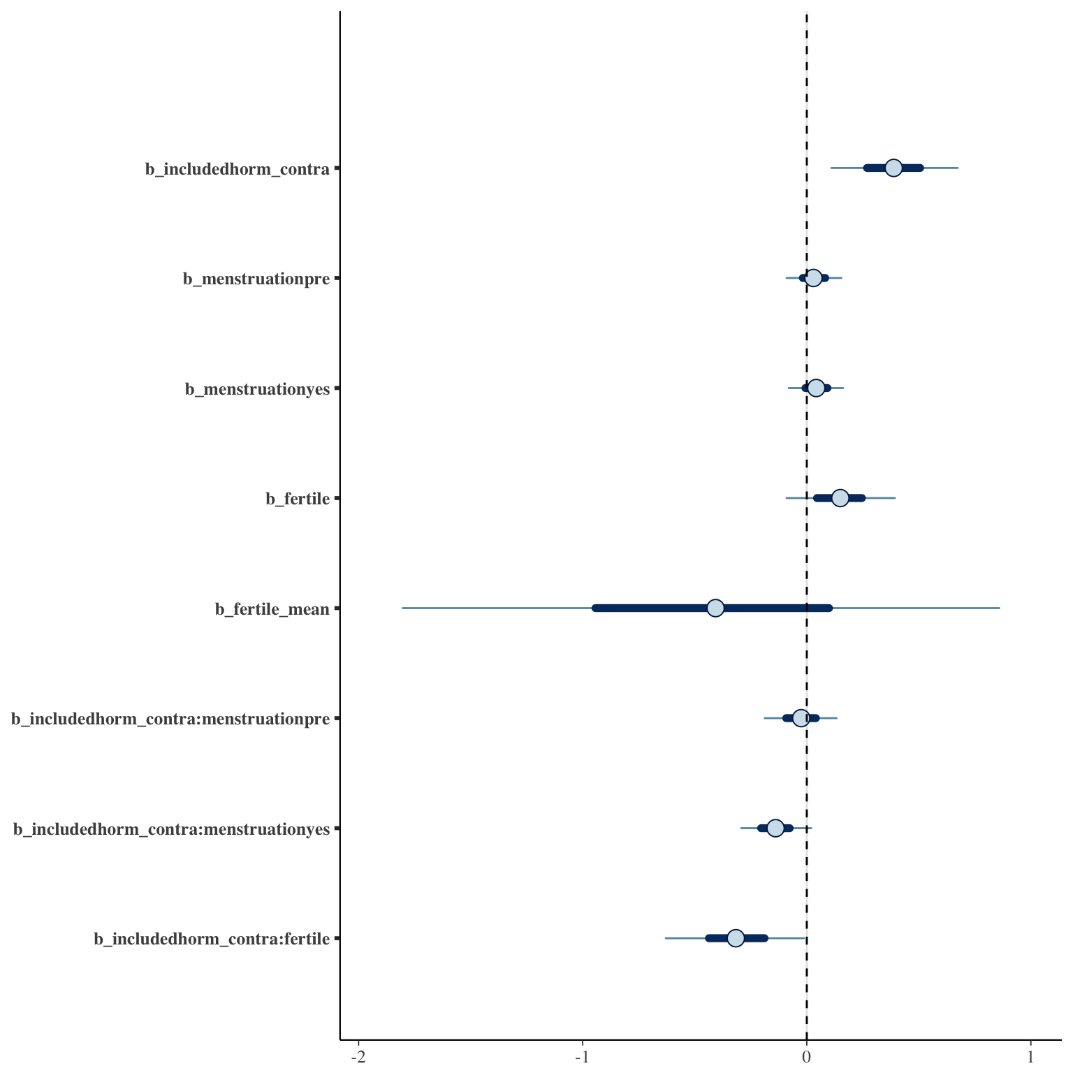
Marginal effect plots
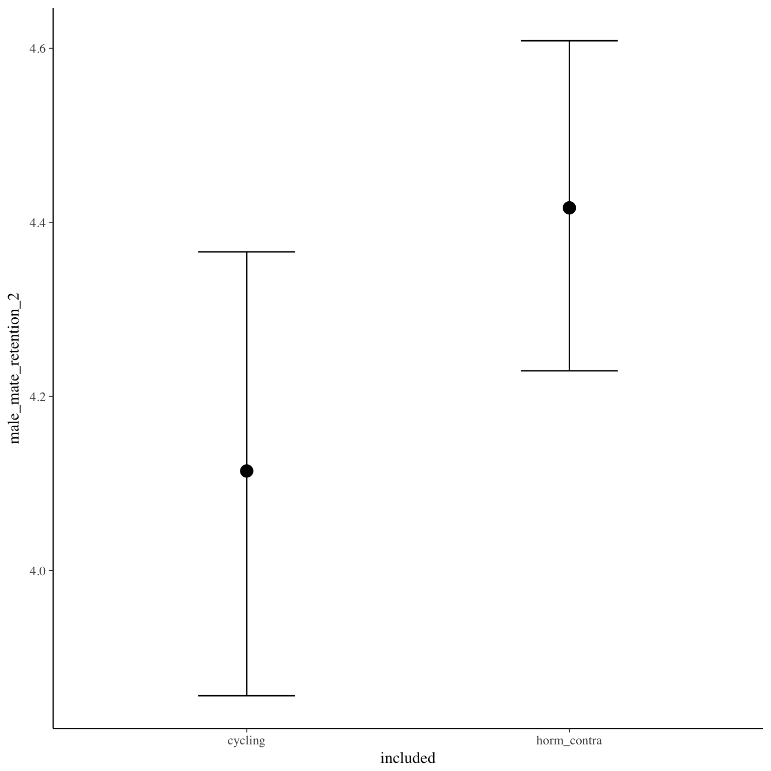
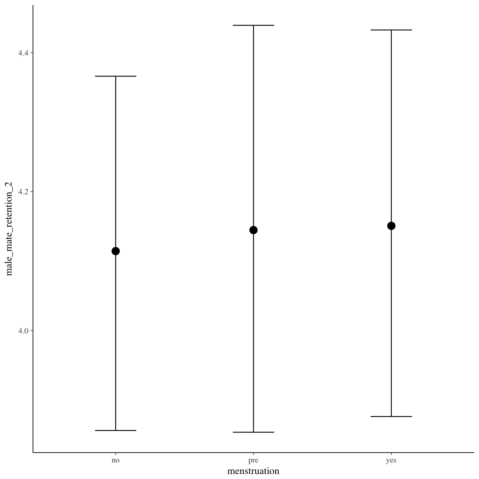
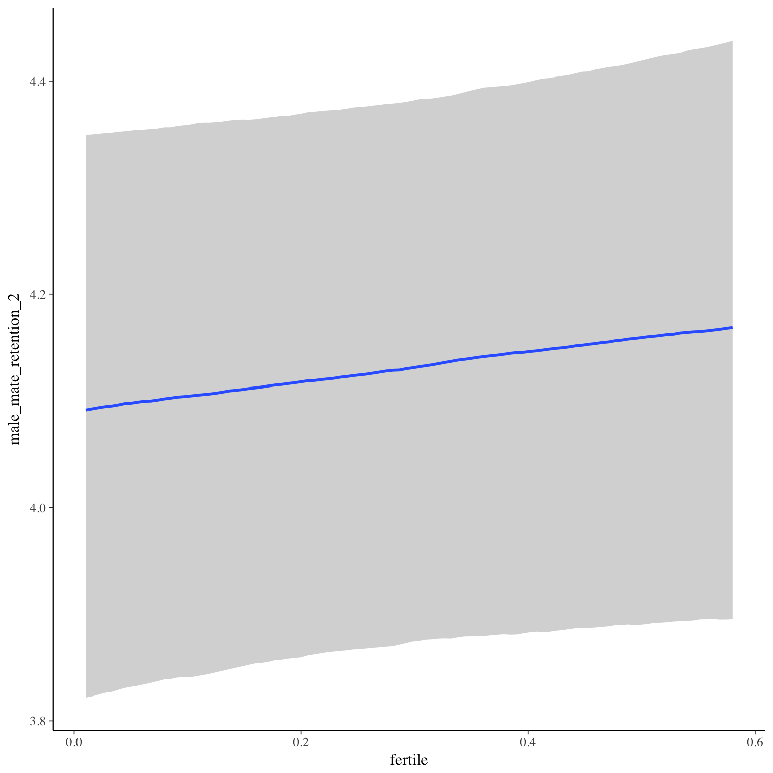
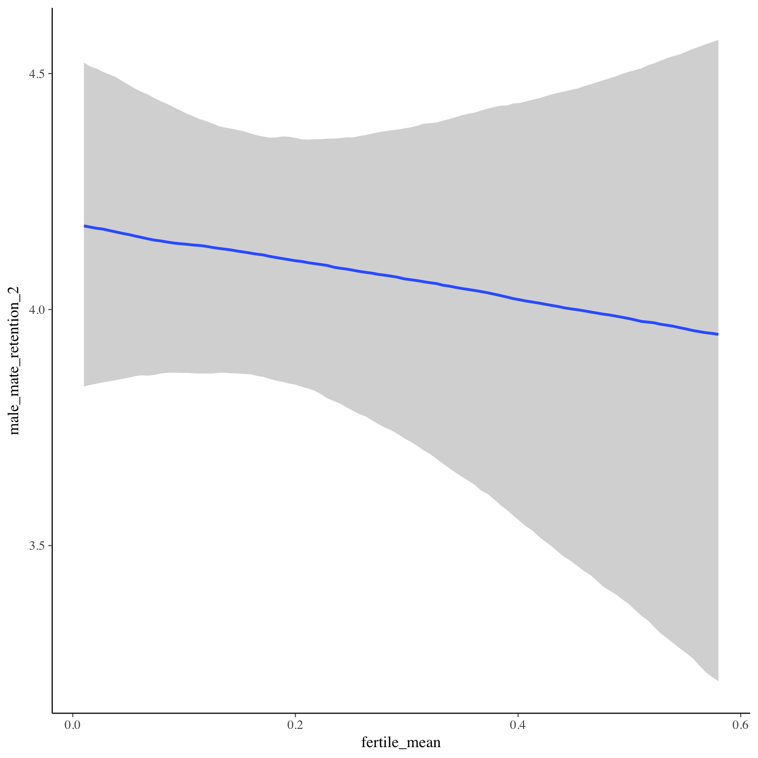
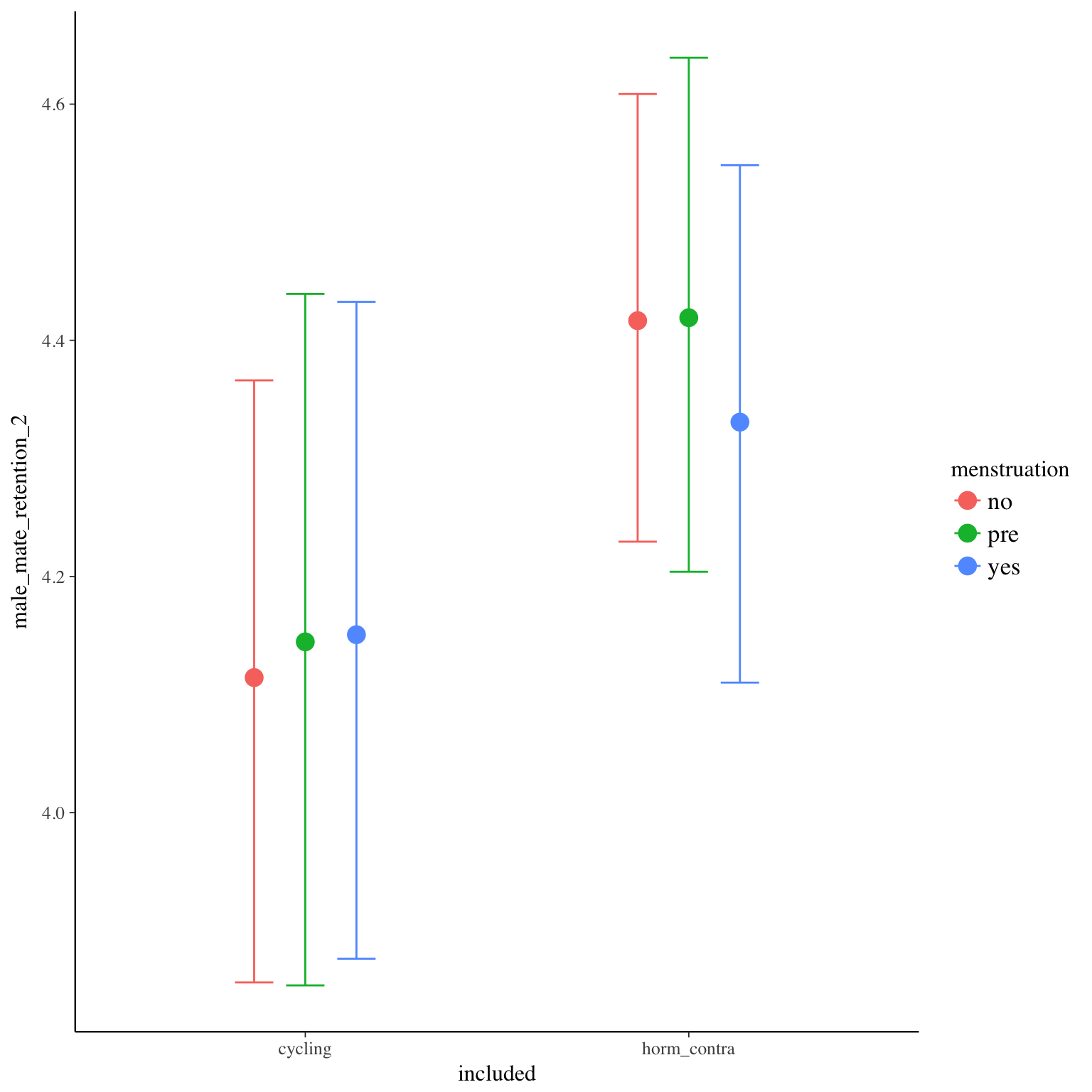
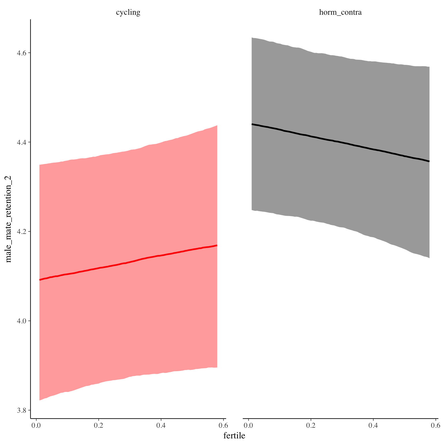
Diagnostics
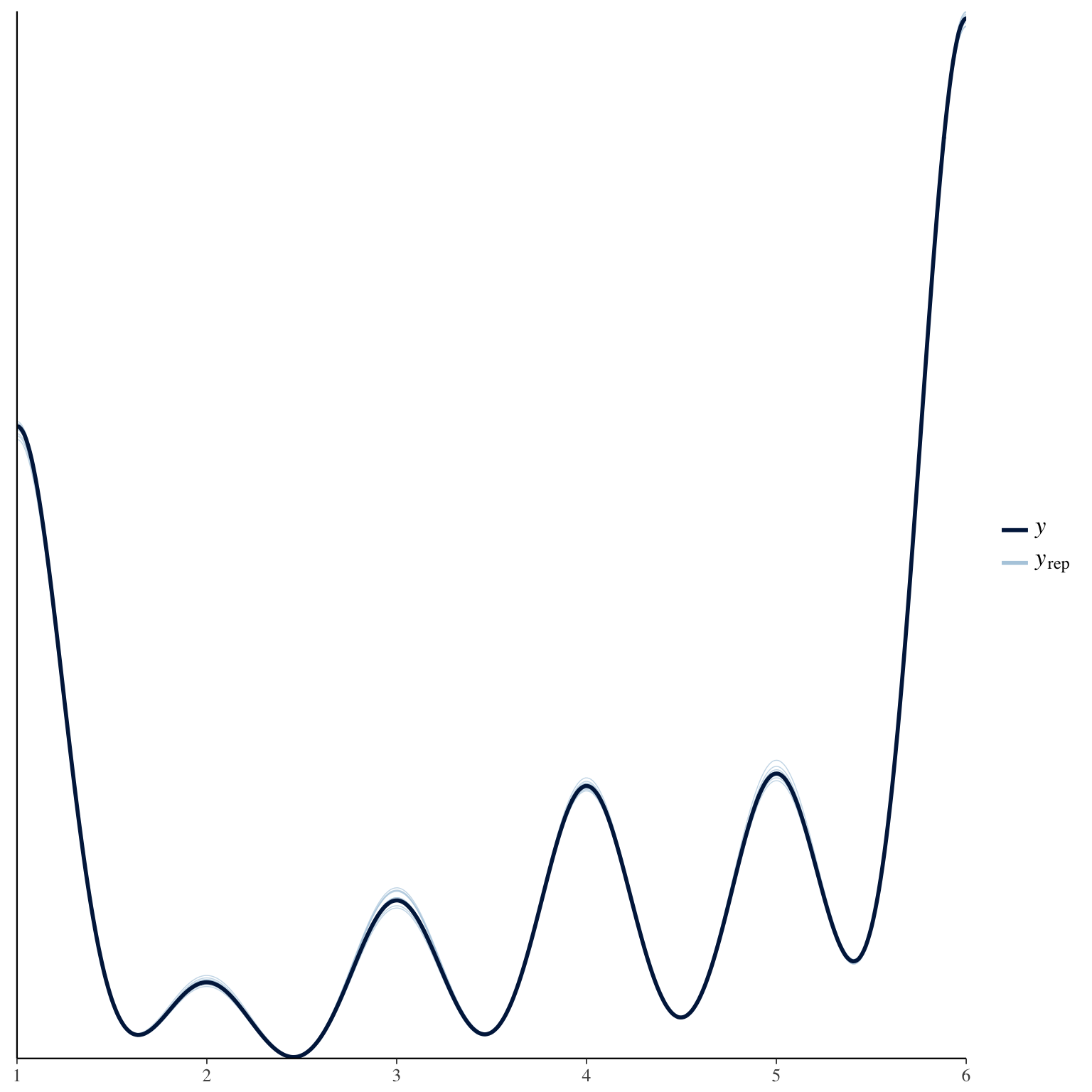
mate_retention_1
Item text:
Haben Sie die letzte Nacht mit Ihrem Partner verbracht?
Item translation:
3. Did you spend last night with your partner?
Choices:
| choice | value | frequency | percent |
|---|---|---|---|
| 1 | ja | 16379 | 0.55 |
| 2 | nein | 13523 | 0.45 |

Model
Model summary
 Family: bernoulli(logit)
Formula: mate_retention_1 ~ included * (menstruation + fertile) + fertile_mean + (1 + fertile + menstruation | person)
   Data: diary (Number of observations: 26568)
Samples: 4 chains, each with iter = 2000; warmup = 1000; thin = 1;
         total post-warmup samples = 4000
    ICs: LOO = 24630.06; WAIC = Not computed

Group-Level Effects:
~person (Number of levels: 1043)
                                     Estimate Est.Error l-95% CI u-95% CI Eff.Sample Rhat
sd(Intercept)                            2.15      0.08     1.99     2.32       1122 1.00
sd(fertile)                              2.09      0.19     1.73     2.45        676 1.00
sd(menstruationpre)                      1.08      0.09     0.89     1.25        757 1.00
sd(menstruationyes)                      1.15      0.11     0.95     1.37       1265 1.00
cor(Intercept,fertile)                   0.01      0.10    -0.19     0.20       2131 1.00
cor(Intercept,menstruationpre)          -0.13      0.10    -0.32     0.07       2032 1.00
cor(fertile,menstruationpre)             0.26      0.10     0.05     0.44        537 1.00
cor(Intercept,menstruationyes)           0.30      0.09     0.11     0.48       1701 1.00
cor(fertile,menstruationyes)             0.21      0.10     0.00     0.40        631 1.01
cor(menstruationpre,menstruationyes)     0.52      0.08     0.35     0.67        980 1.00

Population-Level Effects:
                                    Estimate Est.Error l-95% CI u-95% CI Eff.Sample Rhat
Intercept                              -0.64      0.17    -0.97    -0.28        773    1
includedhorm_contra                     0.34      0.16     0.03     0.65        611    1
menstruationpre                        -0.01      0.11    -0.24     0.21       1823    1
menstruationyes                        -0.11      0.12    -0.34     0.12       1817    1
fertile                                 0.24      0.22    -0.16     0.66       2280    1
fertile_mean                           -0.36      0.72    -1.88     0.99       1501    1
includedhorm_contra:menstruationpre     0.16      0.14    -0.10     0.44       1843    1
includedhorm_contra:menstruationyes     0.27      0.14    -0.01     0.55       1925    1
includedhorm_contra:fertile             0.13      0.26    -0.39     0.65       2226    1

Samples were drawn using sampling(NUTS). For each parameter, Eff.Sample
is a crude measure of effective sample size, and Rhat is the potential
scale reduction factor on split chains (at convergence, Rhat = 1).
Coefficient plot
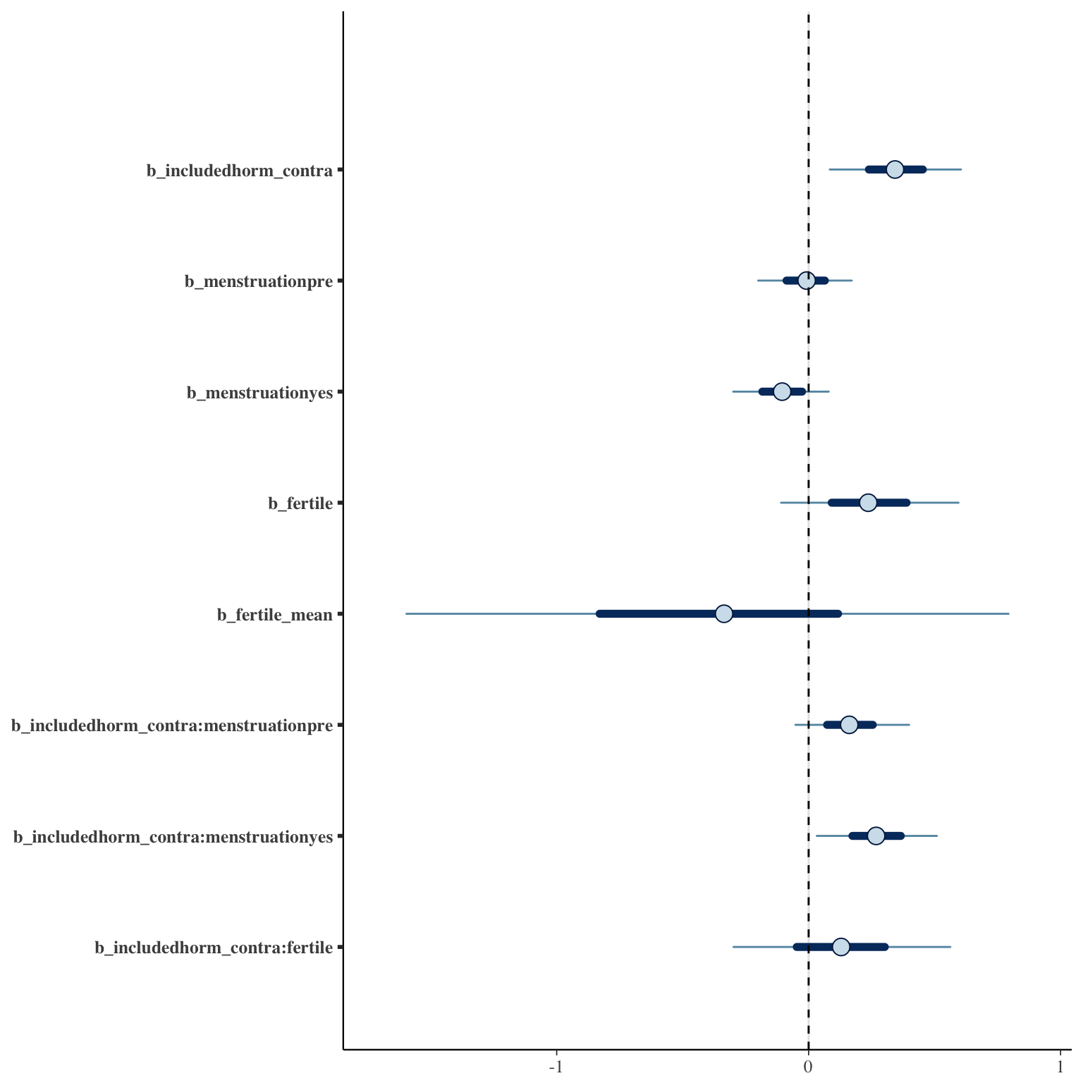
Marginal effect plots
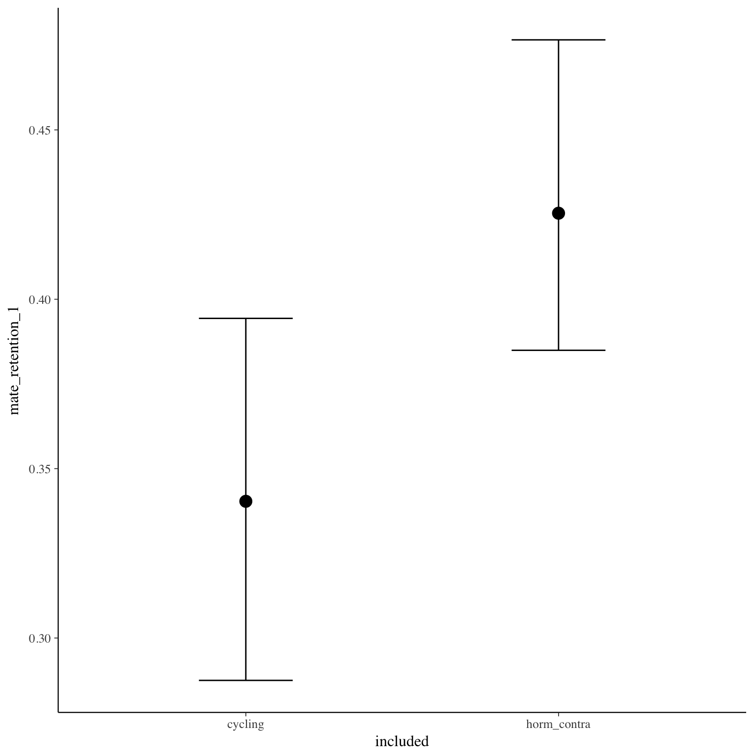
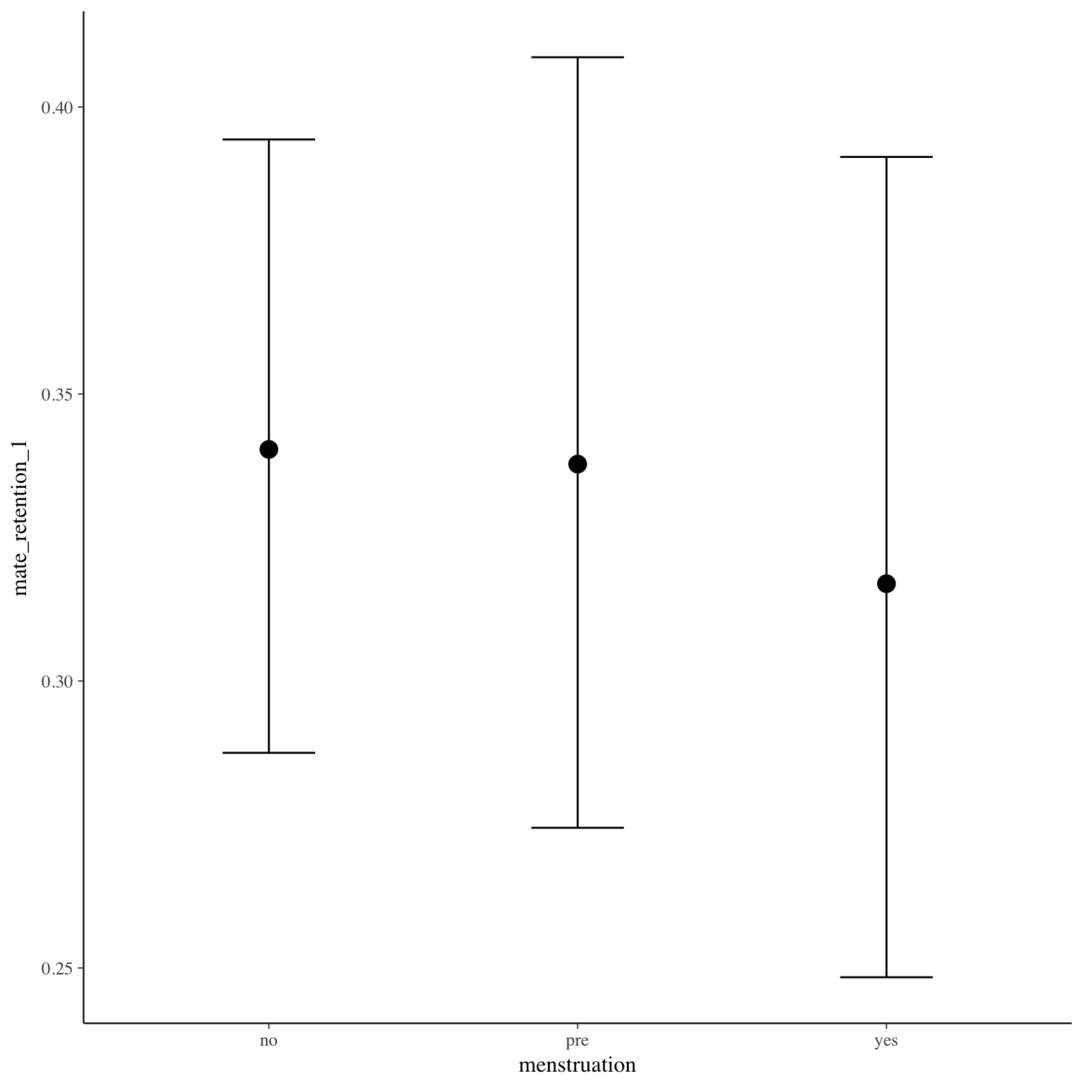
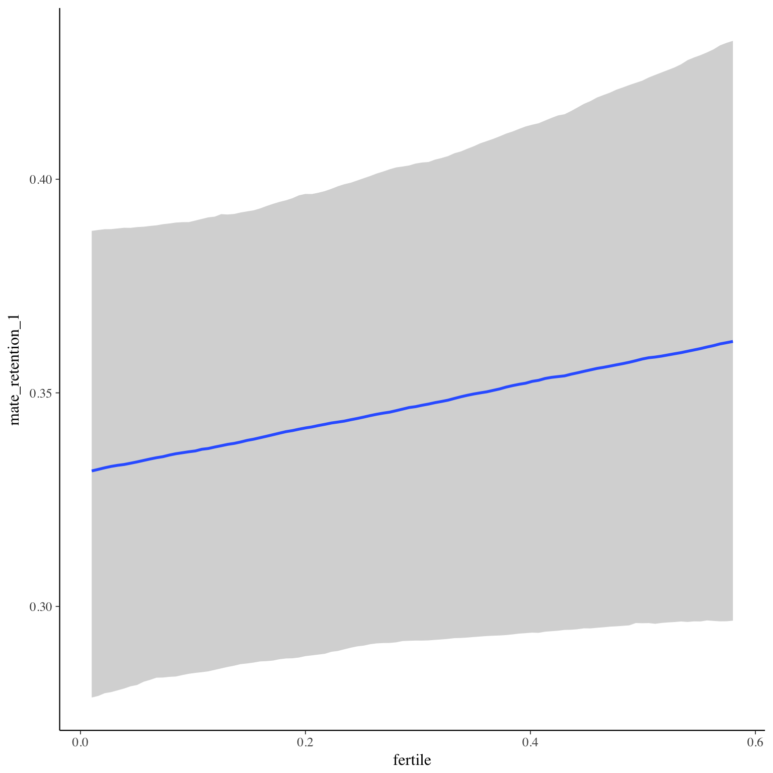
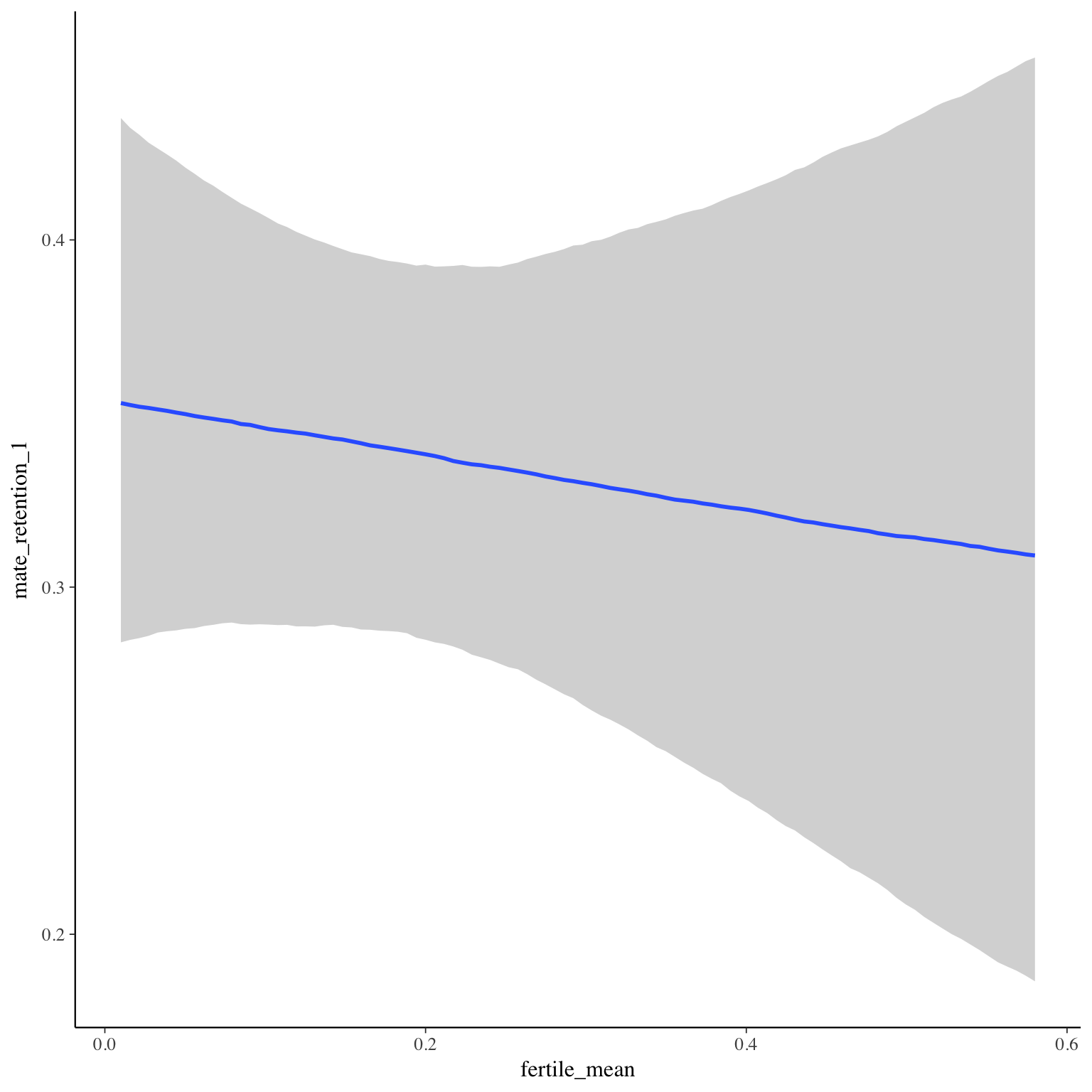
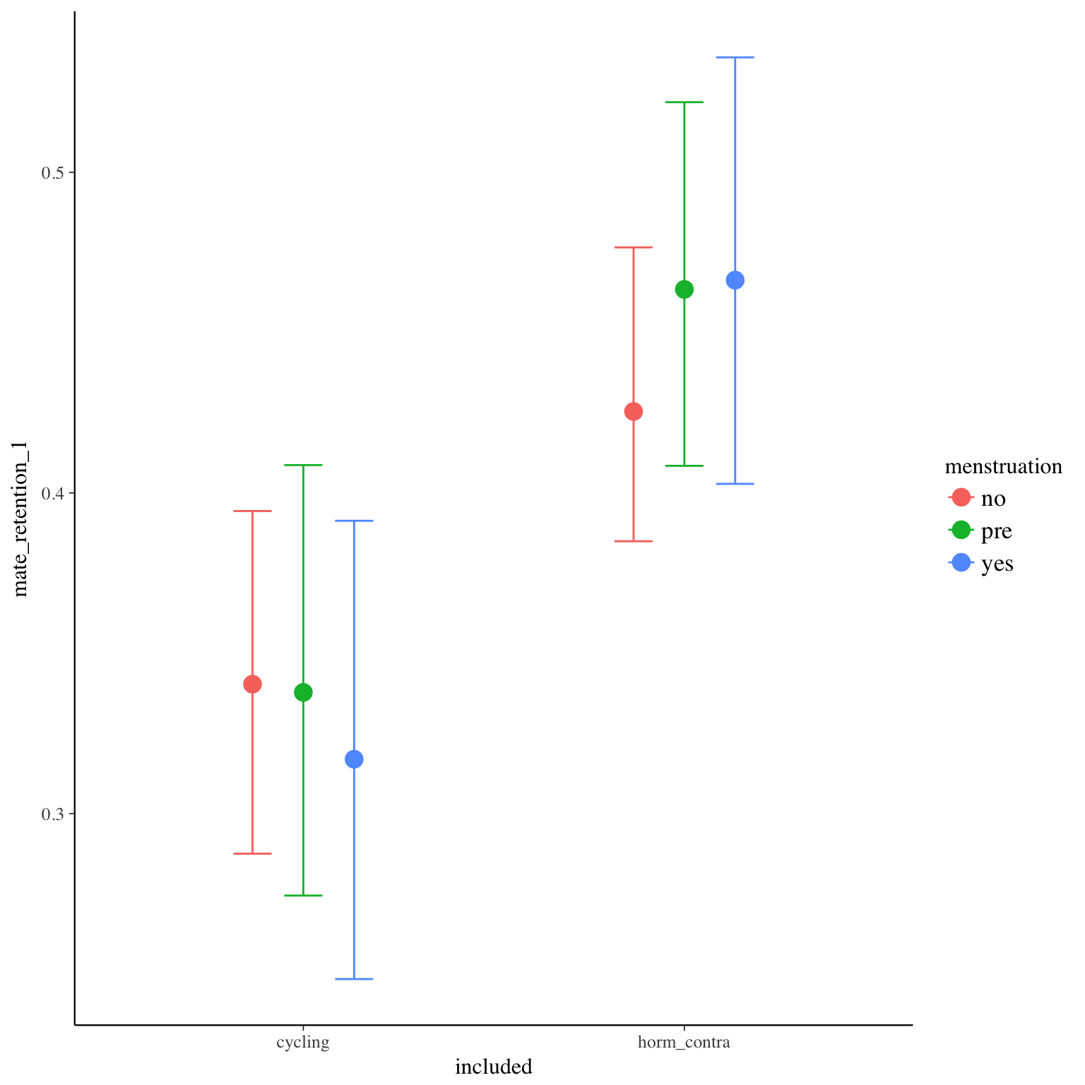
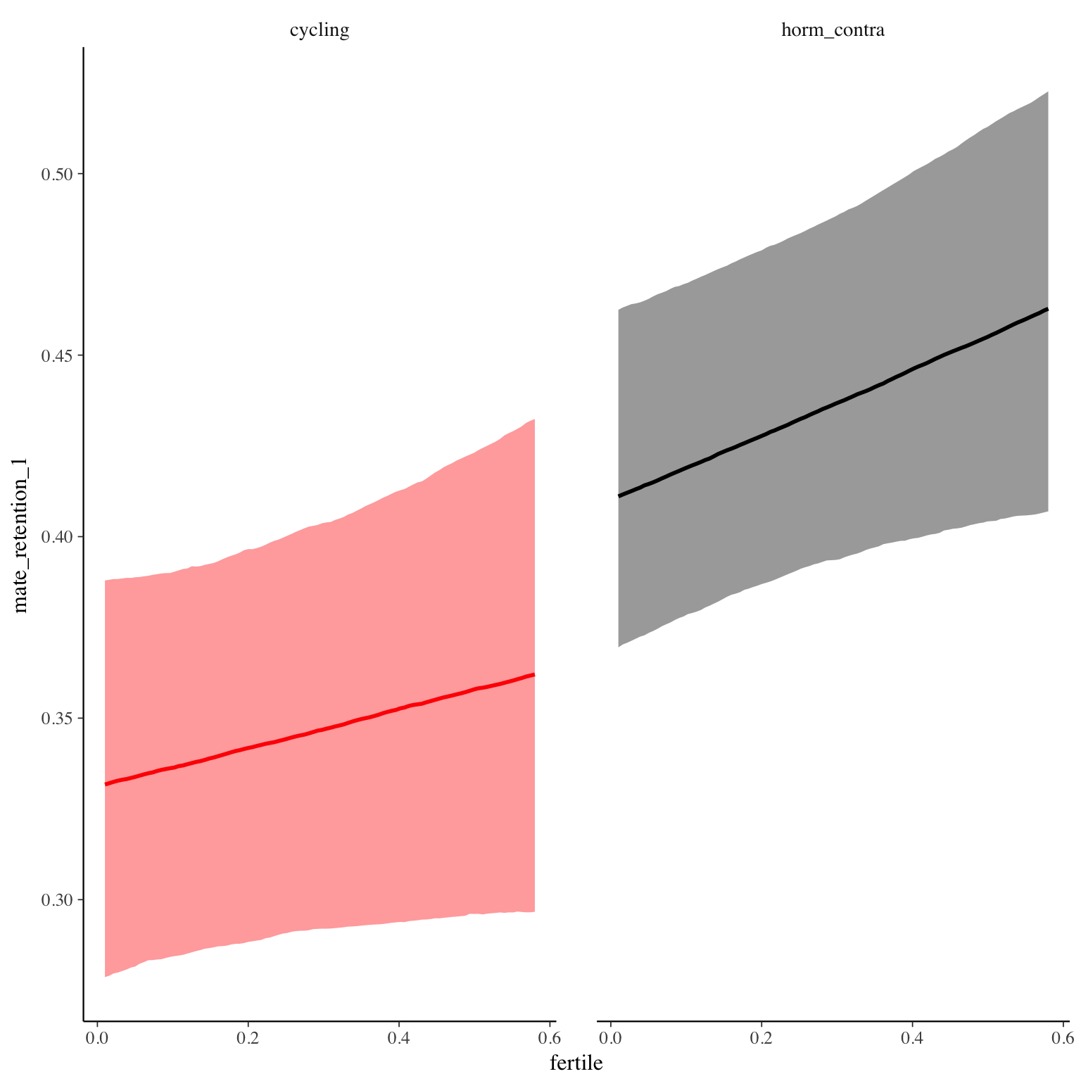
Diagnostics
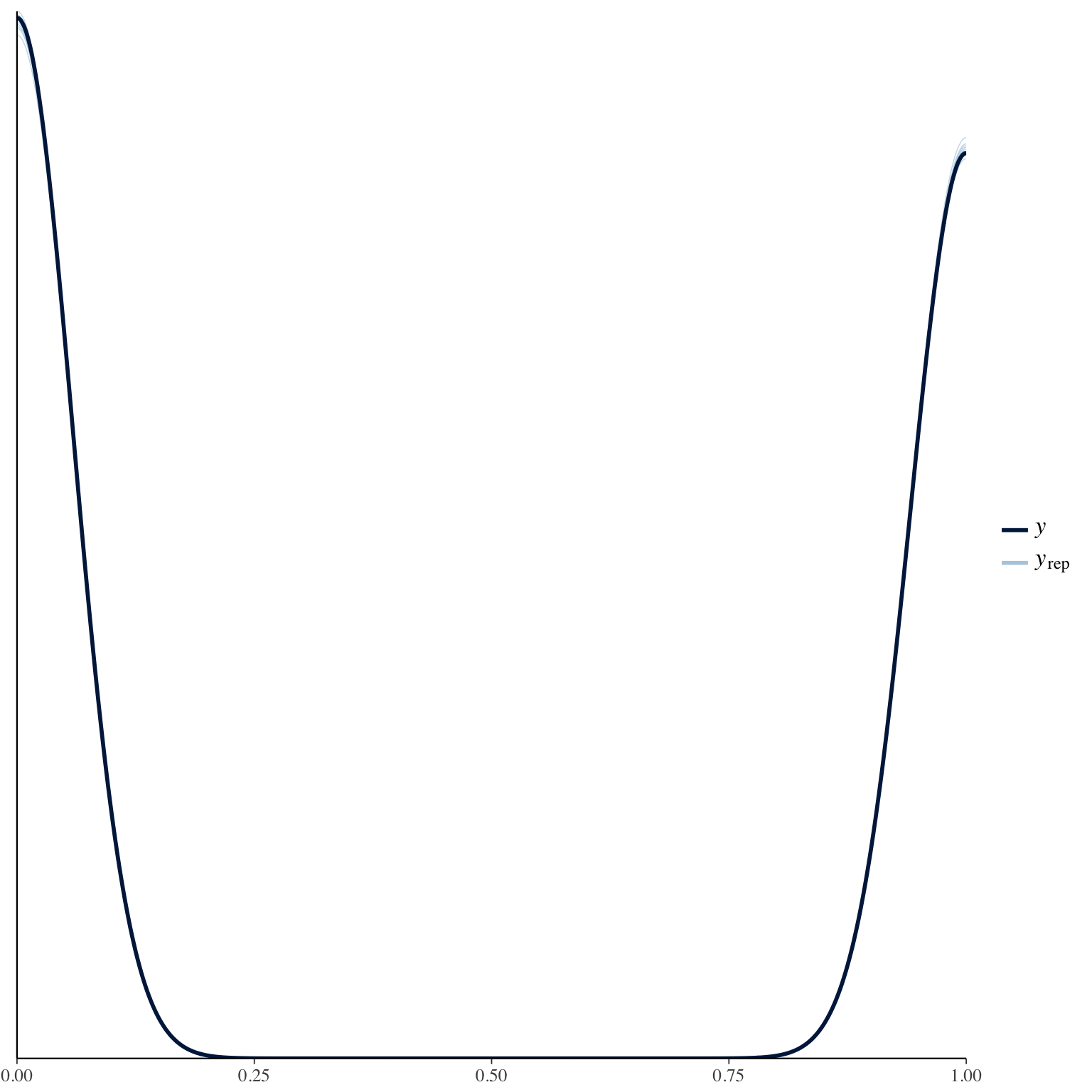
mate_retention_2
Item text:
Haben Sie seit Ihrem letzten Eintrag öffentlich Intimitäten (z.B. Händchenhalten, Küssen, in den Arm nehmen) ausgetauscht?
Item translation:
5. Did you display any forms of public affection (e.g. holding hands, kissing, hugging) with your partner?
Choices:
| choice | value | frequency | percent |
|---|---|---|---|
| 0 | NA | 15931 | 0.53 |
| 1 | ja (1x) | 2720 | 0.09 |
| 2 | ja (mehrfach) | 11251 | 0.38 |
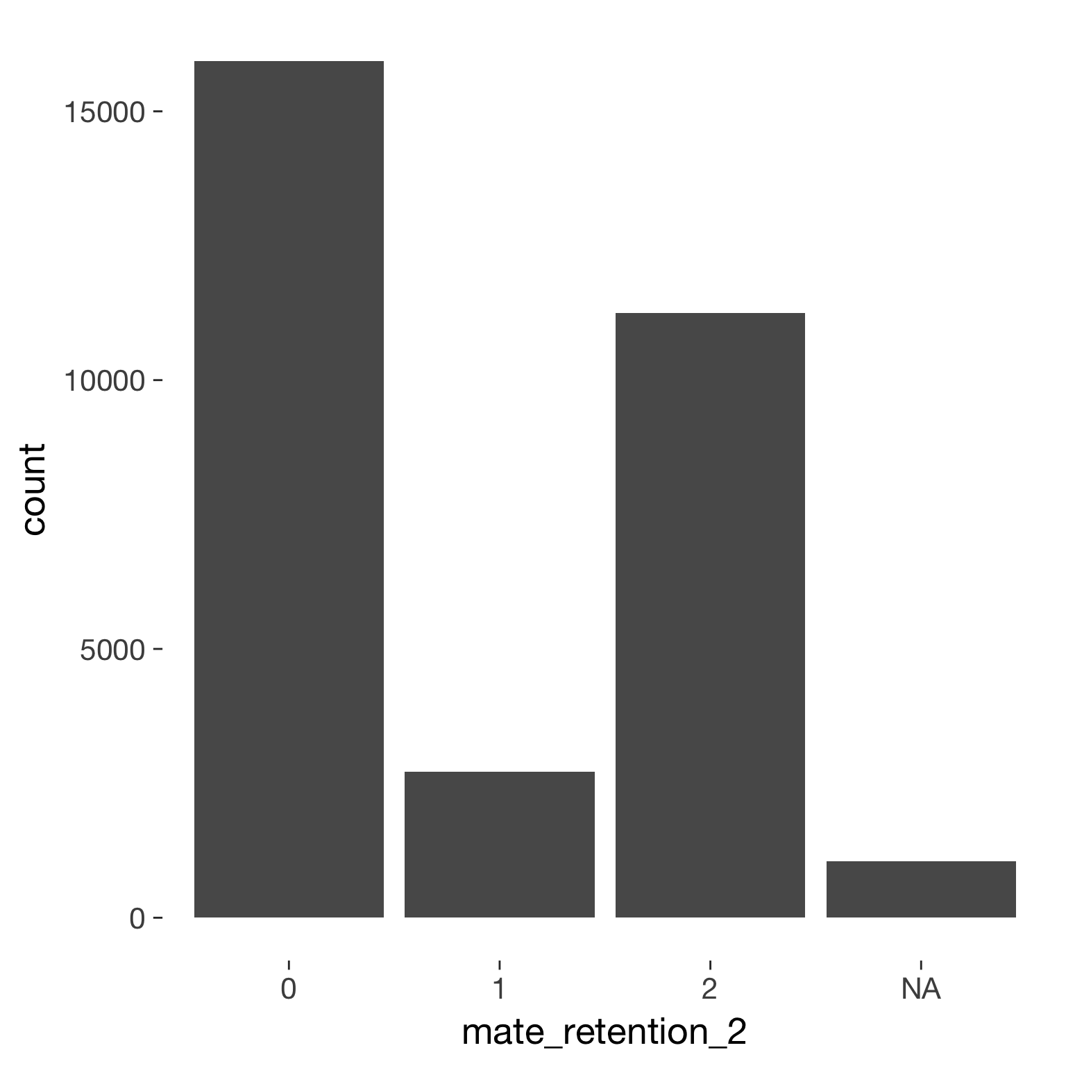
Model
Model summary
 Family: cumulative(logit)
Formula: mate_retention_2 ~ included * (menstruation + fertile) + fertile_mean + (1 + fertile + menstruation | person)
         disc = 1
   Data: diary (Number of observations: 26568)
Samples: 4 chains, each with iter = 2000; warmup = 1000; thin = 1;
         total post-warmup samples = 4000
    ICs: LOO = 42813.55; WAIC = Not computed

Group-Level Effects:
~person (Number of levels: 1043)
                                     Estimate Est.Error l-95% CI u-95% CI Eff.Sample Rhat
sd(Intercept)                            1.24      0.05     1.14     1.35       1350 1.00
sd(fertile)                              1.73      0.14     1.45     2.01        670 1.00
sd(menstruationpre)                      0.81      0.07     0.67     0.95        703 1.01
sd(menstruationyes)                      0.95      0.07     0.80     1.09        994 1.00
cor(Intercept,fertile)                  -0.28      0.08    -0.43    -0.12       1886 1.00
cor(Intercept,menstruationpre)          -0.29      0.08    -0.44    -0.12       1807 1.00
cor(fertile,menstruationpre)             0.20      0.11    -0.03     0.39        619 1.00
cor(Intercept,menstruationyes)           0.07      0.09    -0.09     0.23       1148 1.00
cor(fertile,menstruationyes)             0.18      0.10    -0.02     0.37        598 1.00
cor(menstruationpre,menstruationyes)     0.39      0.09     0.21     0.57        584 1.01

Population-Level Effects:
                                    Estimate Est.Error l-95% CI u-95% CI Eff.Sample Rhat
Intercept[1]                            0.19      0.11    -0.04     0.42       1436    1
Intercept[2]                            0.65      0.11     0.43     0.89       1445    1
includedhorm_contra                     0.07      0.10    -0.12     0.27        973    1
menstruationpre                        -0.04      0.08    -0.20     0.12       2100    1
menstruationyes                        -0.01      0.08    -0.17     0.16       2047    1
fertile                                -0.21      0.16    -0.52     0.11       2124    1
fertile_mean                            0.23      0.49    -0.71     1.19       2064    1
includedhorm_contra:menstruationpre    -0.07      0.10    -0.27     0.13       2164    1
includedhorm_contra:menstruationyes    -0.20      0.11    -0.41     0.01       2188    1
includedhorm_contra:fertile            -0.30      0.21    -0.70     0.11       2017    1

Samples were drawn using sampling(NUTS). For each parameter, Eff.Sample
is a crude measure of effective sample size, and Rhat is the potential
scale reduction factor on split chains (at convergence, Rhat = 1).
Coefficient plot
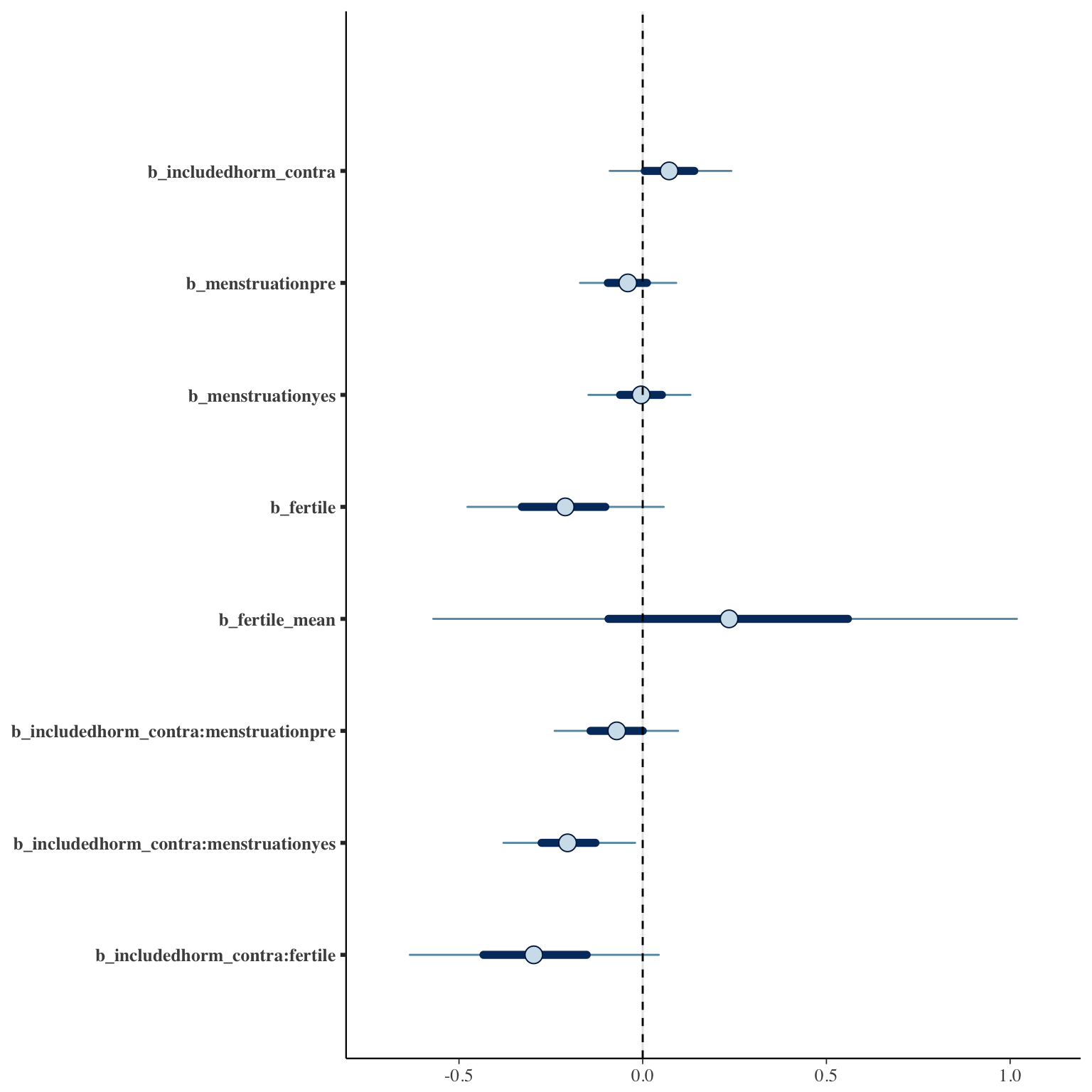
Marginal effect plots
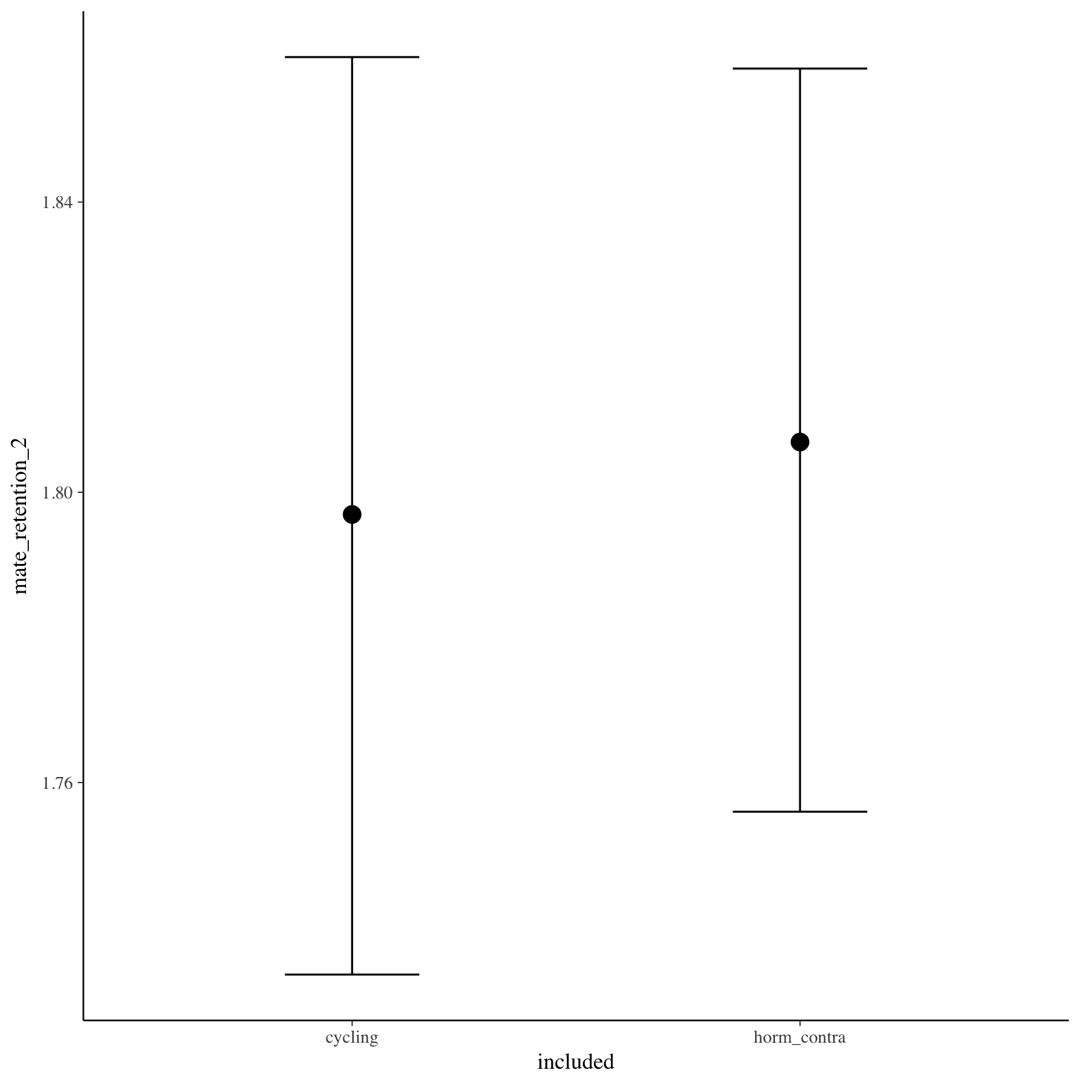
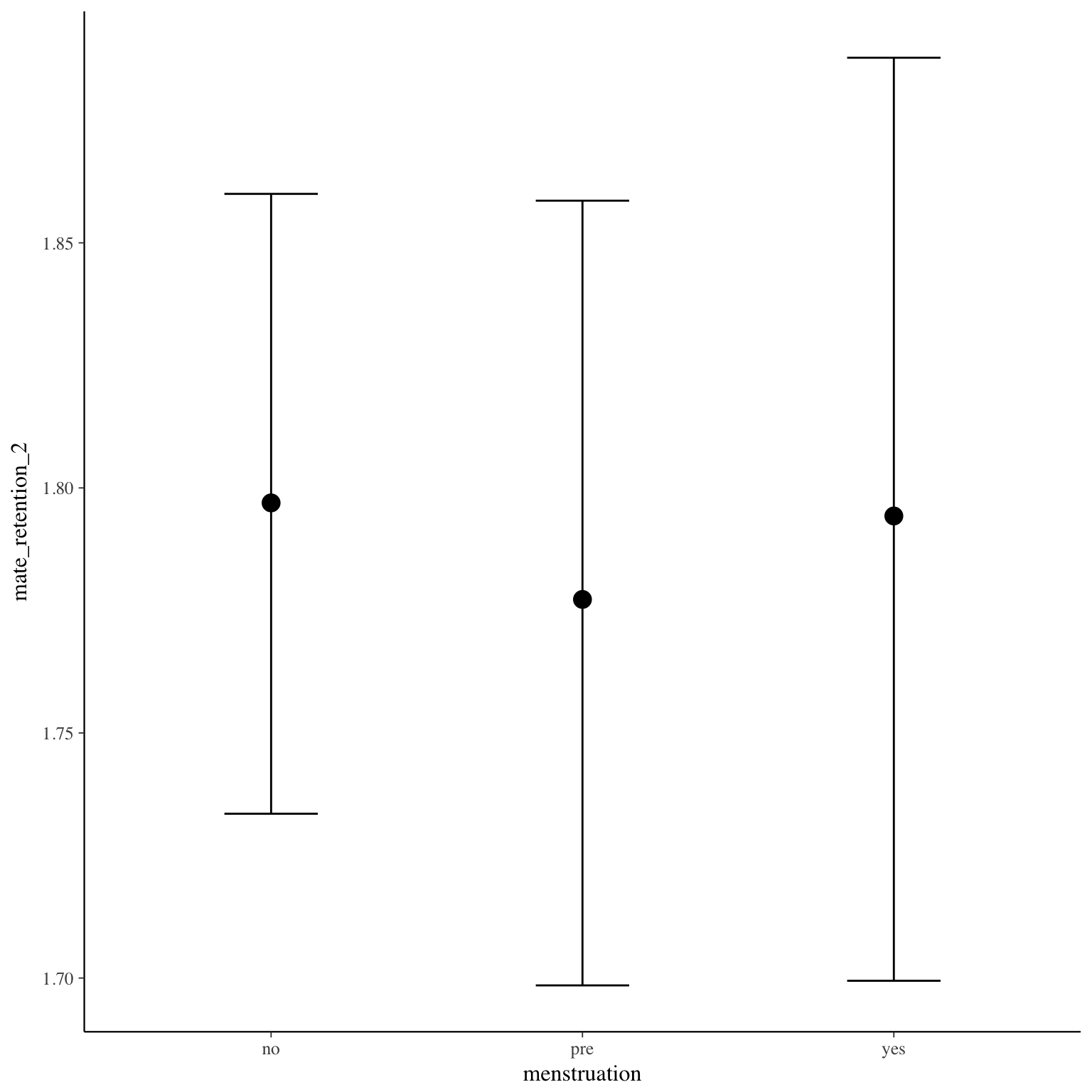
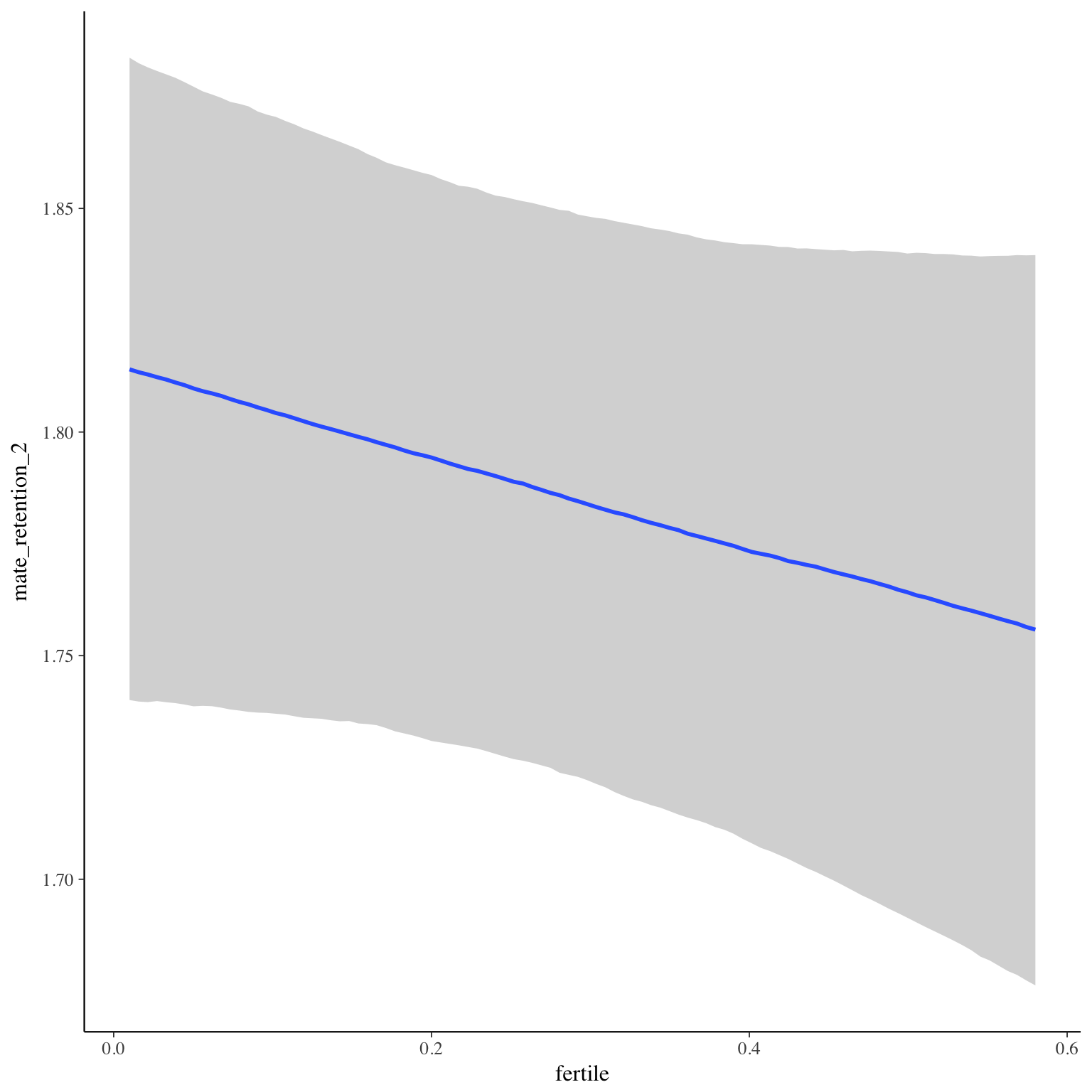
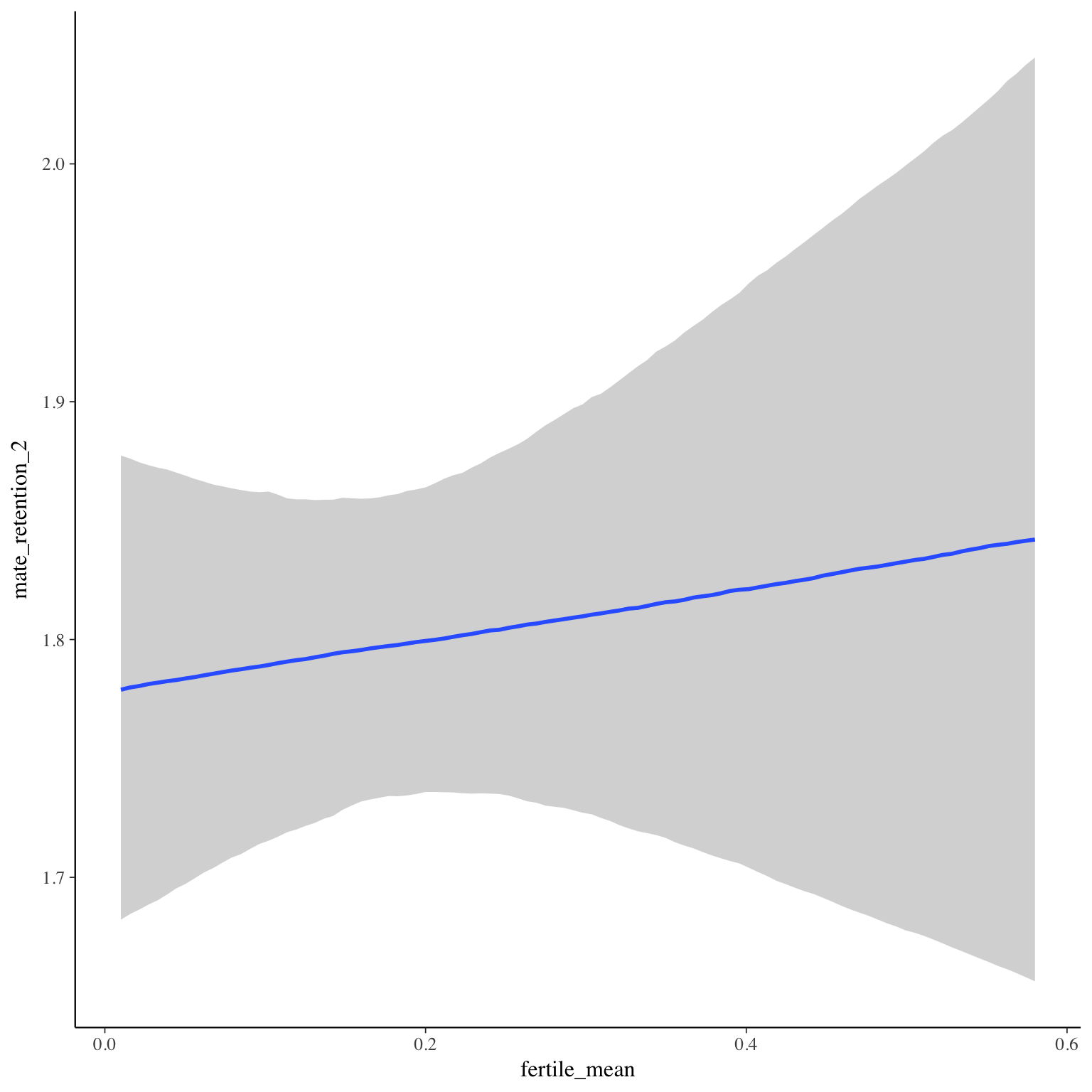
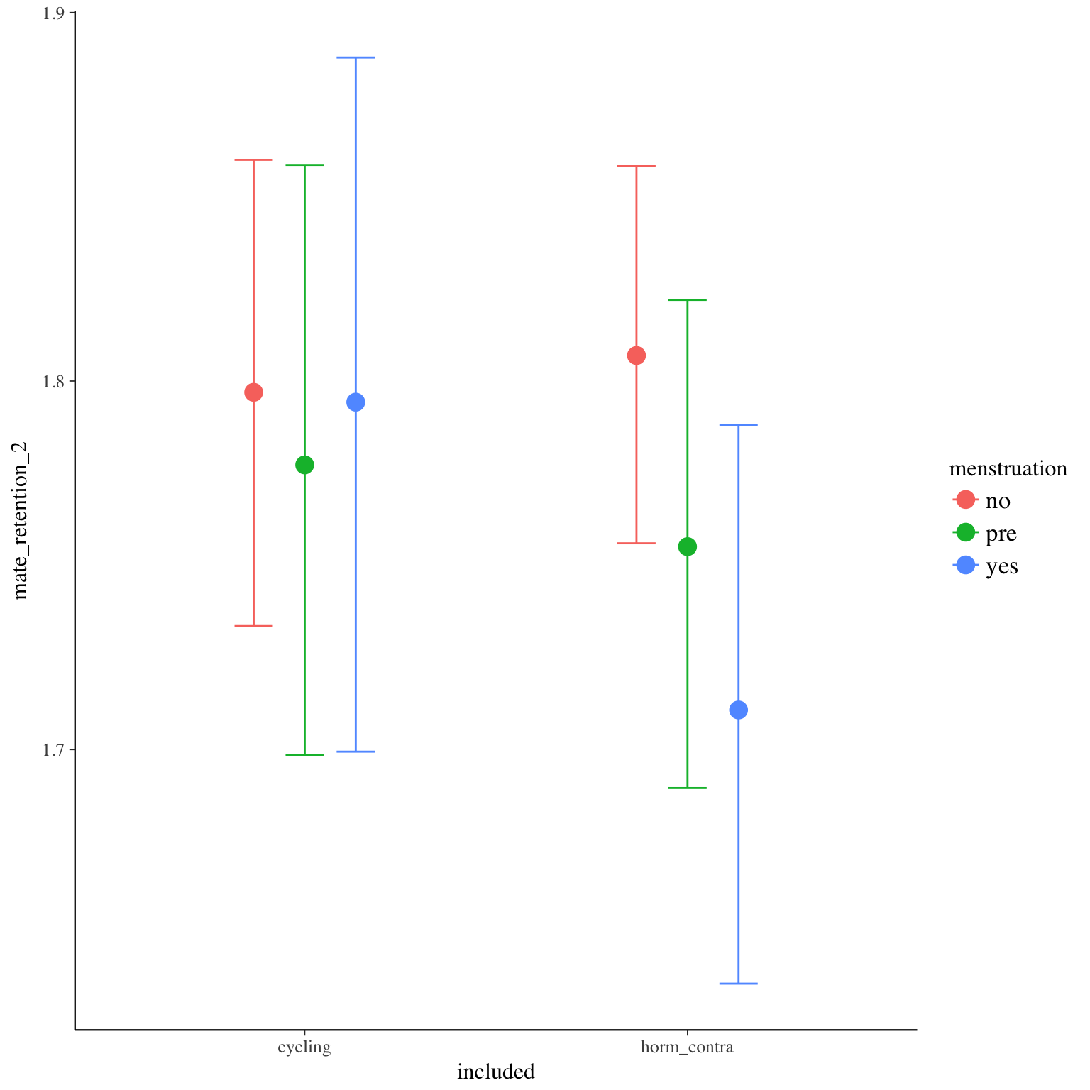
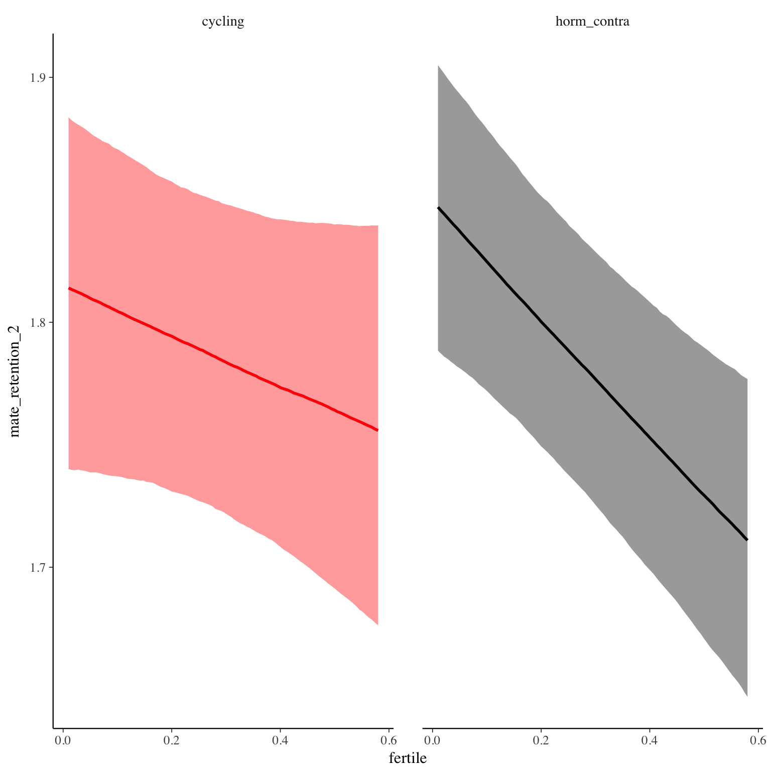
Diagnostics
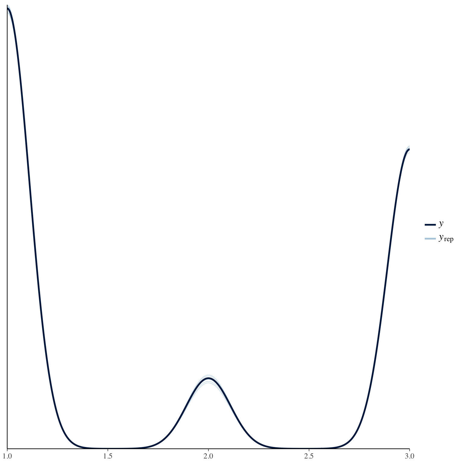
mate_retention_3
Item text:
… habe ich mich für meinen Partner besonders hübsch gemacht.
Item translation:
37. I made myself up especially for my partner.
Choices:
| choice | value | frequency | percent |
|---|---|---|---|
| 1 | Stimme nicht zu | 10603 | 0.35 |
| 2 | Stimme überwiegend nicht zu | 2841 | 0.1 |
| 3 | Stimme eher nicht zu | 4843 | 0.16 |
| 4 | Stimme eher zu | 5519 | 0.18 |
| 5 | Stimme überwiegend zu | 3674 | 0.12 |
| 6 | Stimme voll zu | 2396 | 0.08 |
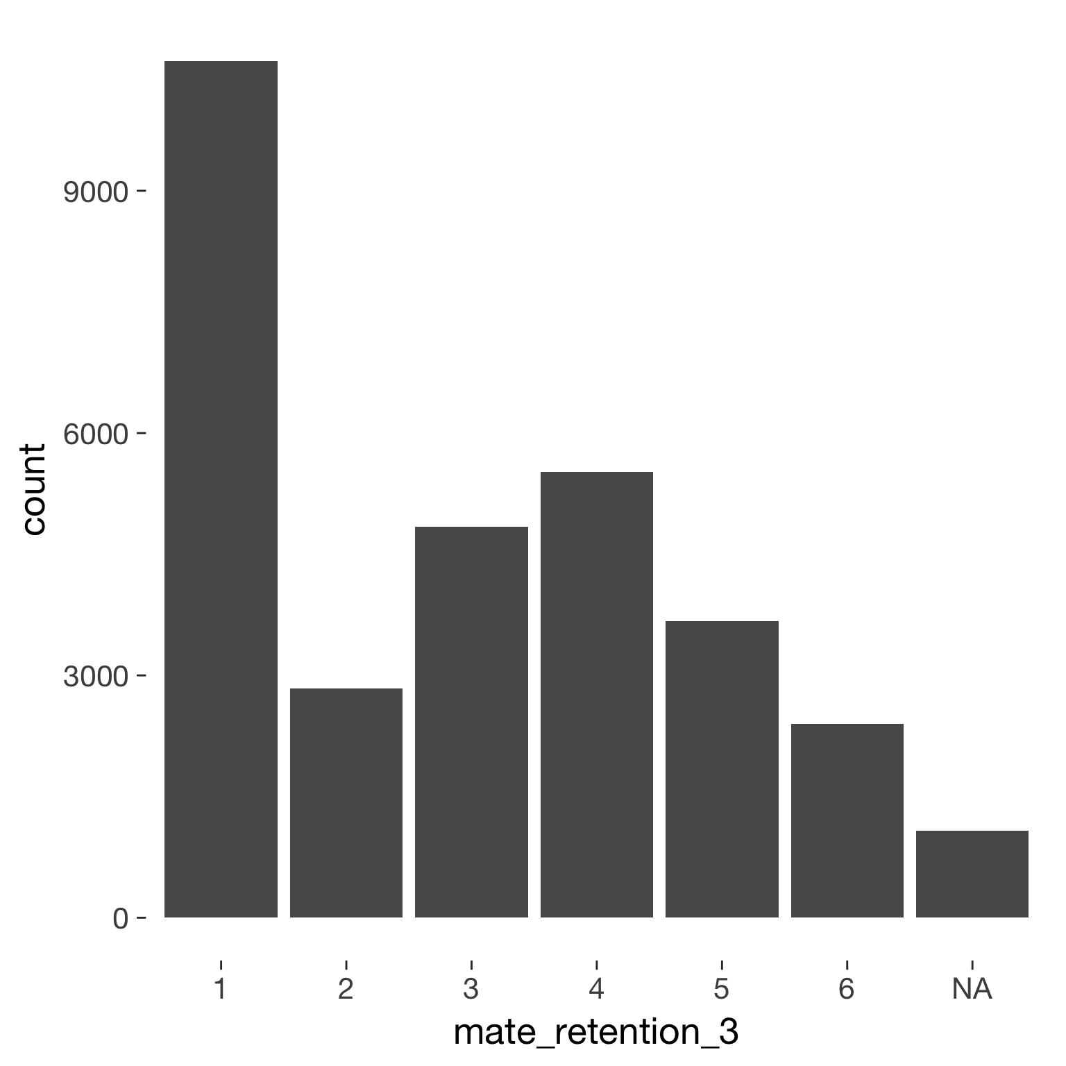
Model
Model summary
 Family: cumulative(logit)
Formula: mate_retention_3 ~ included * (menstruation + fertile) + fertile_mean + (1 + fertile + menstruation | person)
         disc = 1
   Data: diary (Number of observations: 26545)
Samples: 4 chains, each with iter = 2000; warmup = 1000; thin = 1;
         total post-warmup samples = 4000
    ICs: LOO = 78990.97; WAIC = Not computed

Group-Level Effects:
~person (Number of levels: 1043)
                                     Estimate Est.Error l-95% CI u-95% CI Eff.Sample Rhat
sd(Intercept)                            1.42      0.05     1.34     1.52       1201 1.00
sd(fertile)                              1.67      0.12     1.44     1.91        592 1.00
sd(menstruationpre)                      0.61      0.07     0.48     0.74        747 1.00
sd(menstruationyes)                      0.78      0.06     0.66     0.90        651 1.00
cor(Intercept,fertile)                  -0.26      0.06    -0.38    -0.13       1727 1.00
cor(Intercept,menstruationpre)          -0.25      0.08    -0.41    -0.08       2122 1.00
cor(fertile,menstruationpre)             0.38      0.10     0.17     0.56        825 1.00
cor(Intercept,menstruationyes)          -0.19      0.07    -0.33    -0.05       1996 1.00
cor(fertile,menstruationyes)             0.48      0.08     0.31     0.63        676 1.01
cor(menstruationpre,menstruationyes)     0.46      0.10     0.25     0.66        463 1.01

Population-Level Effects:
                                    Estimate Est.Error l-95% CI u-95% CI Eff.Sample Rhat
Intercept[1]                           -0.61      0.13    -0.87    -0.37        775    1
Intercept[2]                           -0.06      0.13    -0.32     0.19        771    1
Intercept[3]                            0.81      0.13     0.56     1.06        772    1
Intercept[4]                            1.95      0.13     1.69     2.20        773    1
Intercept[5]                            3.20      0.13     2.94     3.45        799    1
includedhorm_contra                     0.22      0.11     0.00     0.44        655    1
menstruationpre                        -0.06      0.07    -0.20     0.08       2169    1
menstruationyes                        -0.14      0.07    -0.28     0.01       1603    1
fertile                                 0.03      0.15    -0.27     0.33       1435    1
fertile_mean                           -0.11      0.52    -1.17     0.89       1469    1
includedhorm_contra:menstruationpre     0.02      0.09    -0.16     0.19       1812    1
includedhorm_contra:menstruationyes     0.09      0.09    -0.08     0.28       1485    1
includedhorm_contra:fertile            -0.27      0.19    -0.65     0.09       1449    1

Samples were drawn using sampling(NUTS). For each parameter, Eff.Sample
is a crude measure of effective sample size, and Rhat is the potential
scale reduction factor on split chains (at convergence, Rhat = 1).
Coefficient plot
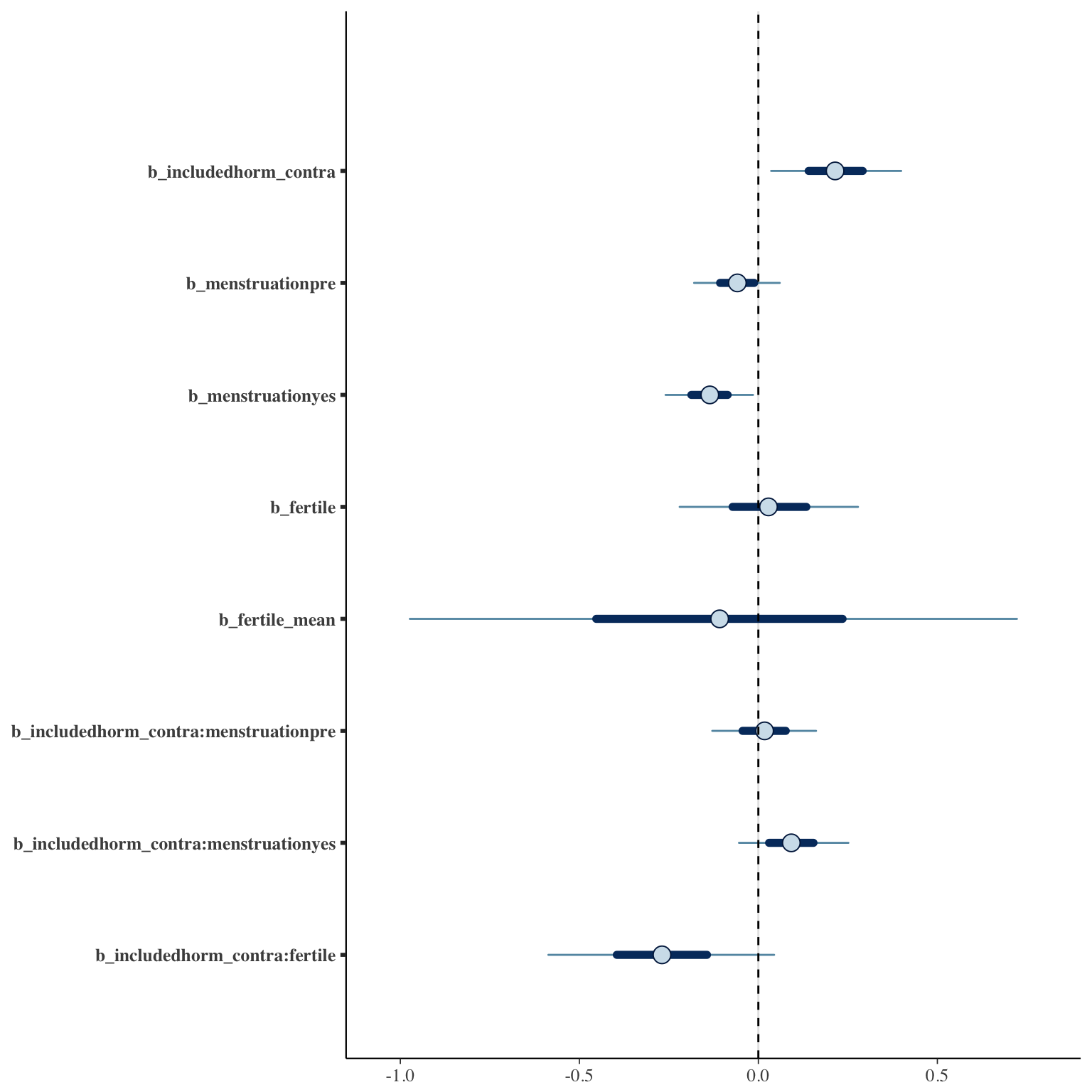
Marginal effect plots

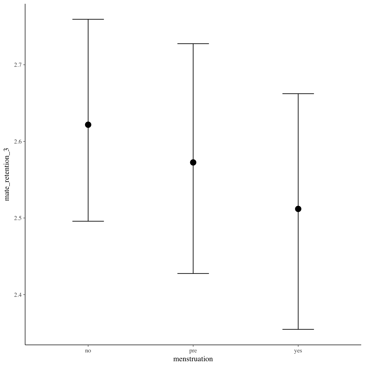
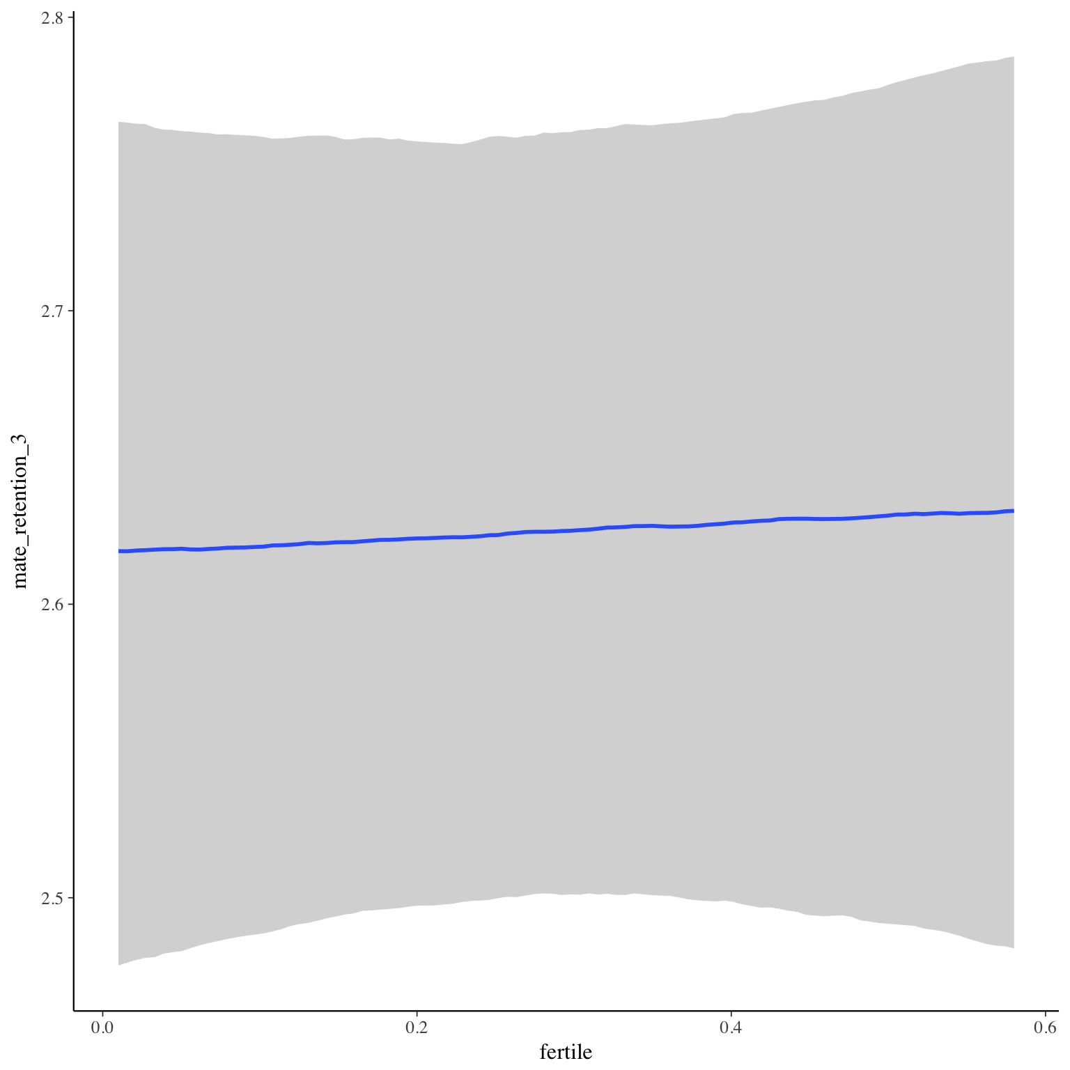
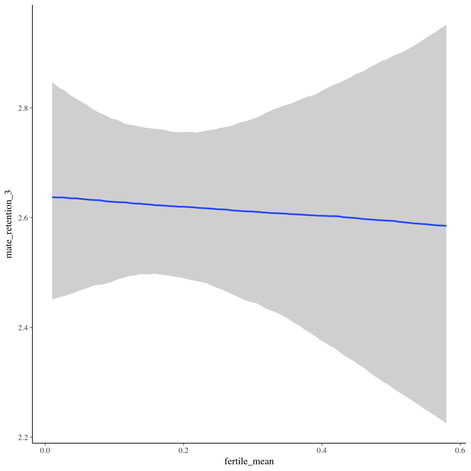
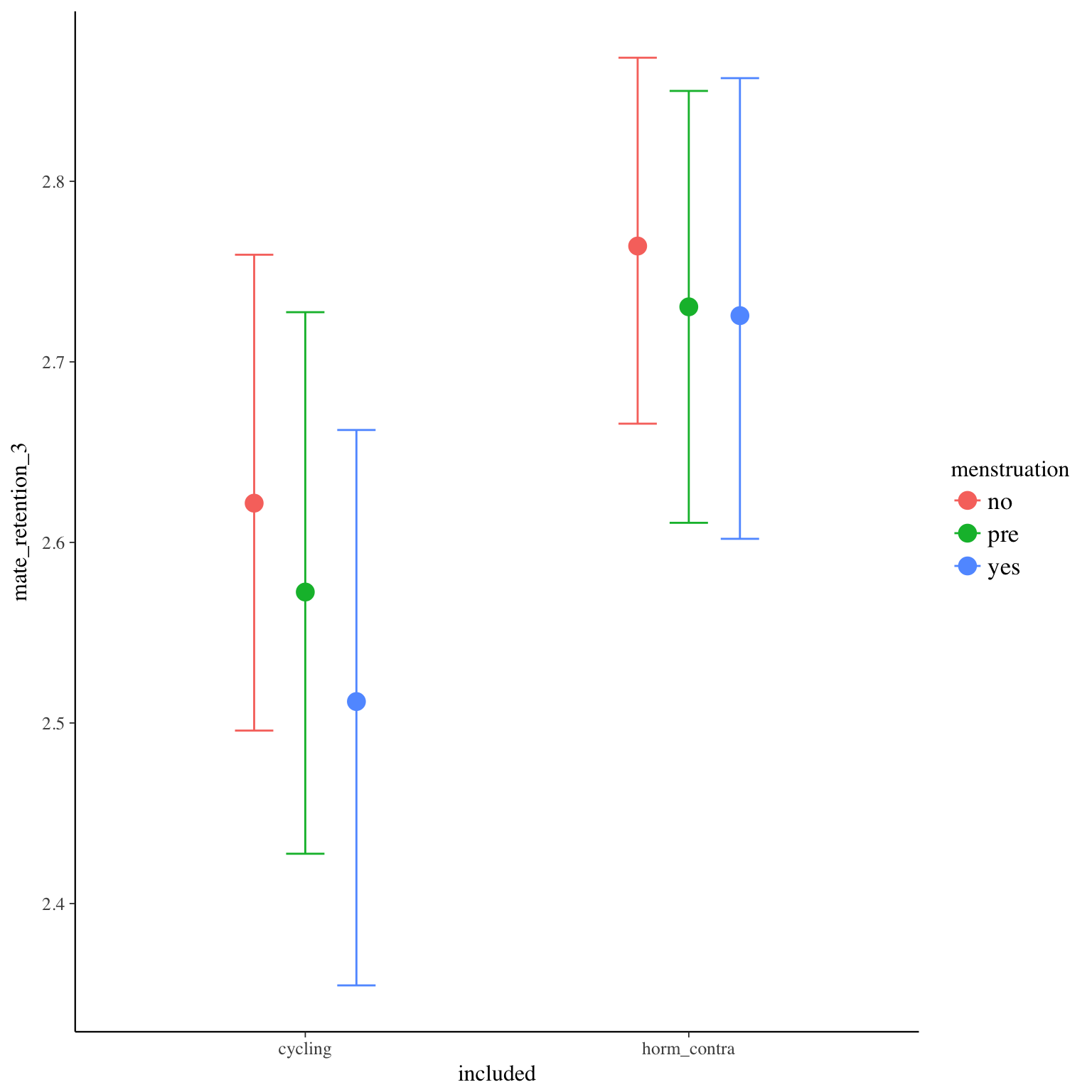
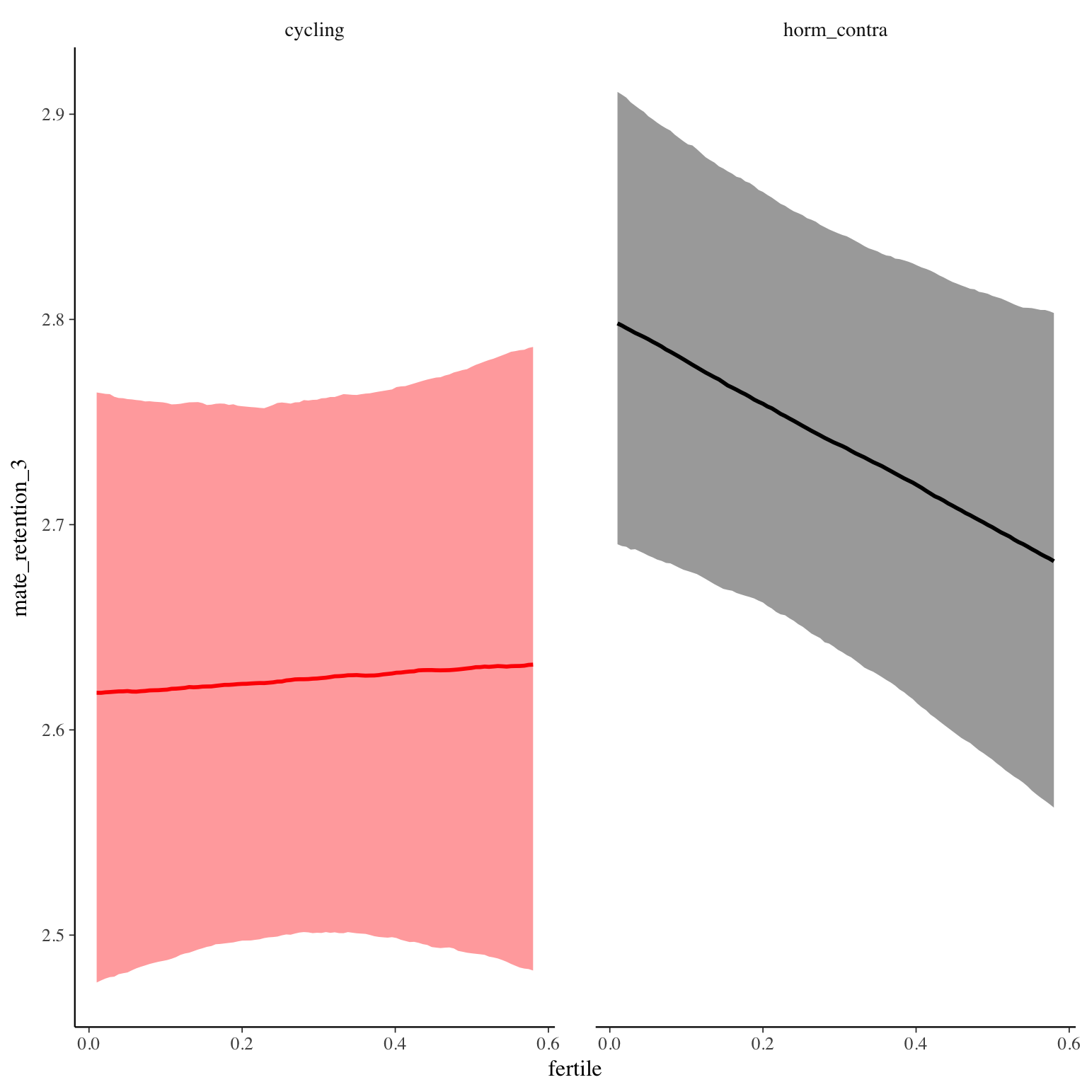
Diagnostics
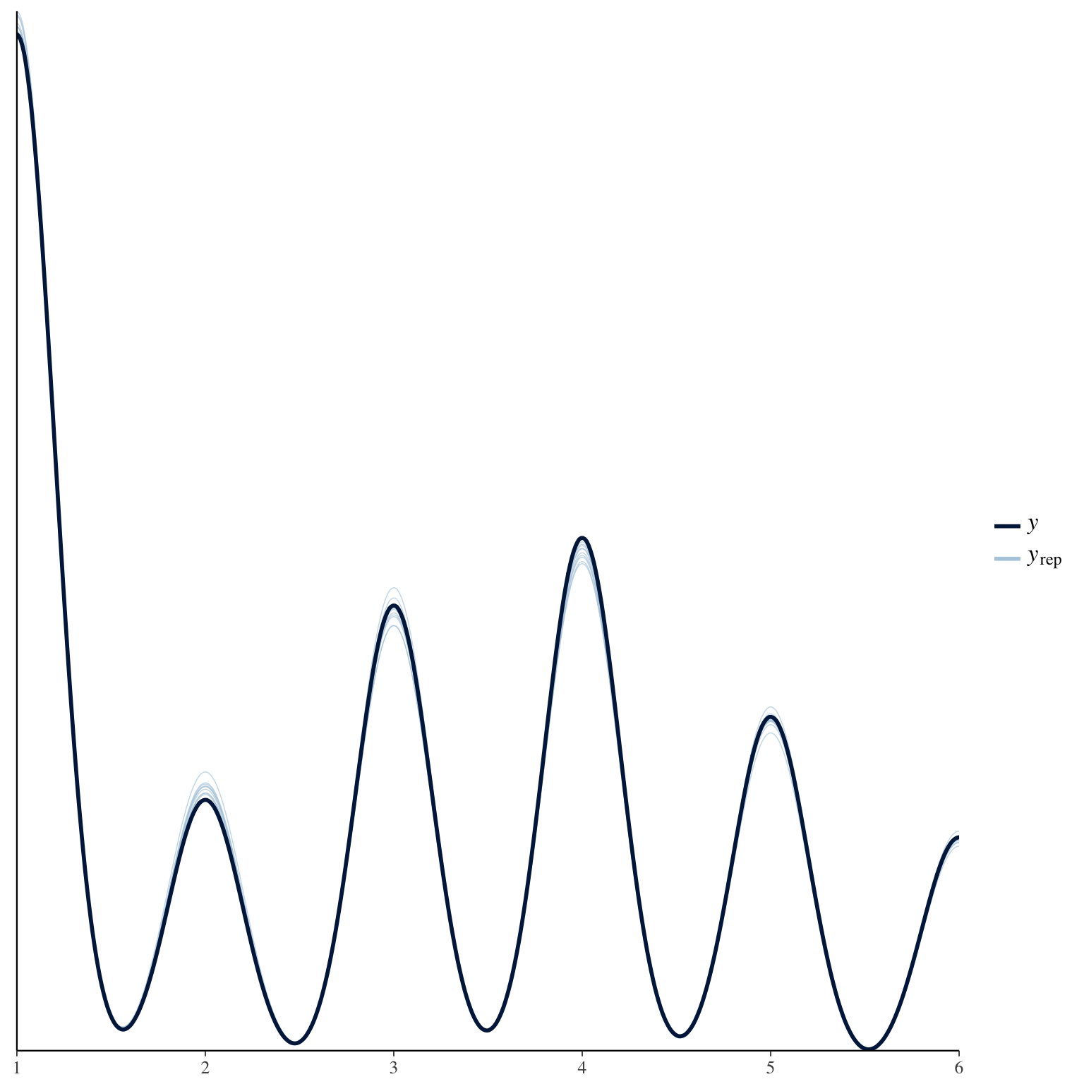
mate_retention_4
Item text:
… habe ich meinem Partner gesagt, dass ich ihn liebe.
Item translation:
38. I told my partner I love him.
Choices:
| choice | value | frequency | percent |
|---|---|---|---|
| 1 | Stimme nicht zu | 7577 | 0.25 |
| 2 | Stimme überwiegend nicht zu | 1239 | 0.04 |
| 3 | Stimme eher nicht zu | 2205 | 0.07 |
| 4 | Stimme eher zu | 3522 | 0.12 |
| 5 | Stimme überwiegend zu | 3550 | 0.12 |
| 6 | Stimme voll zu | 11783 | 0.39 |
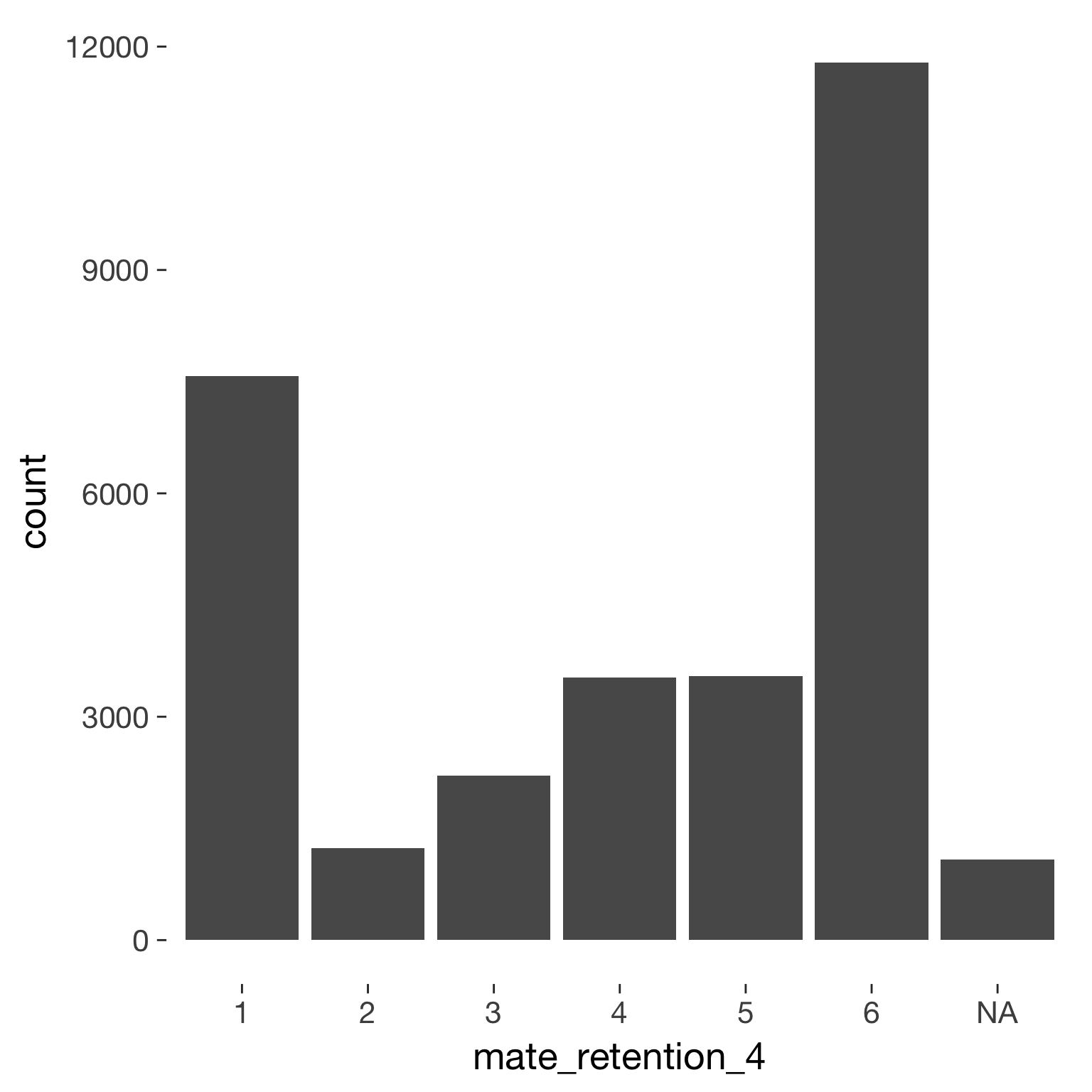
Model
Model summary
 Family: cumulative(logit)
Formula: mate_retention_4 ~ included * (menstruation + fertile) + fertile_mean + (1 + fertile + menstruation | person)
         disc = 1
   Data: diary (Number of observations: 26545)
Samples: 4 chains, each with iter = 2000; warmup = 1000; thin = 1;
         total post-warmup samples = 4000
    ICs: LOO = 61074.44; WAIC = Not computed

Group-Level Effects:
~person (Number of levels: 1043)
                                     Estimate Est.Error l-95% CI u-95% CI Eff.Sample Rhat
sd(Intercept)                            2.73      0.09     2.57     2.90        488 1.01
sd(fertile)                              1.01      0.17     0.67     1.32        167 1.03
sd(menstruationpre)                      0.59      0.08     0.42     0.75        346 1.01
sd(menstruationyes)                      0.58      0.08     0.42     0.73        425 1.01
cor(Intercept,fertile)                   0.00      0.15    -0.28     0.29       2702 1.00
cor(Intercept,menstruationpre)           0.26      0.13    -0.01     0.51       1115 1.01
cor(fertile,menstruationpre)            -0.43      0.23    -0.86     0.00        113 1.04
cor(Intercept,menstruationyes)           0.03      0.13    -0.22     0.29       2369 1.00
cor(fertile,menstruationyes)             0.18      0.18    -0.20     0.53        184 1.03
cor(menstruationpre,menstruationyes)     0.33      0.15     0.02     0.61        336 1.02

Population-Level Effects:
                                    Estimate Est.Error l-95% CI u-95% CI Eff.Sample Rhat
Intercept[1]                           -1.93      0.19    -2.32    -1.57        278 1.02
Intercept[2]                           -1.55      0.19    -1.93    -1.19        279 1.02
Intercept[3]                           -0.92      0.19    -1.30    -0.56        280 1.02
Intercept[4]                           -0.01      0.19    -0.39     0.35        280 1.02
Intercept[5]                            0.92      0.19     0.54     1.28        282 1.02
includedhorm_contra                     0.31      0.17    -0.04     0.63        196 1.01
menstruationpre                         0.06      0.08    -0.09     0.21       2268 1.00
menstruationyes                         0.05      0.07    -0.08     0.19       2241 1.00
fertile                                 0.13      0.14    -0.14     0.41       2141 1.00
fertile_mean                           -0.57      0.81    -2.30     0.93        529 1.01
includedhorm_contra:menstruationpre    -0.01      0.10    -0.20     0.19       2131 1.00
includedhorm_contra:menstruationyes    -0.12      0.09    -0.30     0.06       2198 1.00
includedhorm_contra:fertile            -0.33      0.18    -0.69     0.00       2207 1.00

Samples were drawn using sampling(NUTS). For each parameter, Eff.Sample
is a crude measure of effective sample size, and Rhat is the potential
scale reduction factor on split chains (at convergence, Rhat = 1).
Coefficient plot
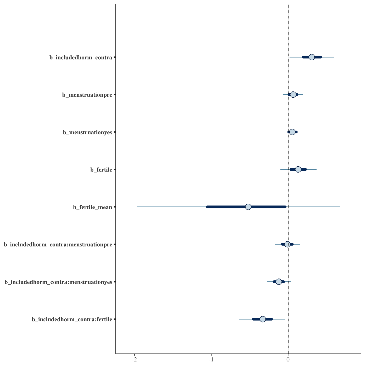
Marginal effect plots

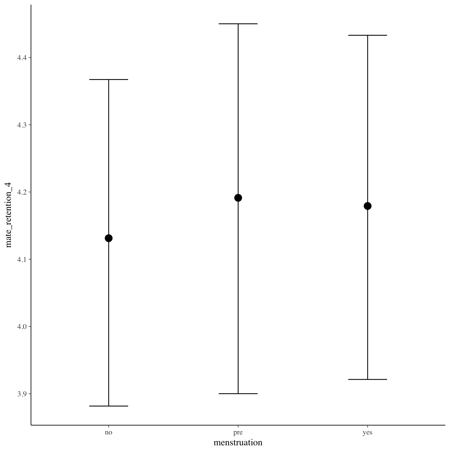
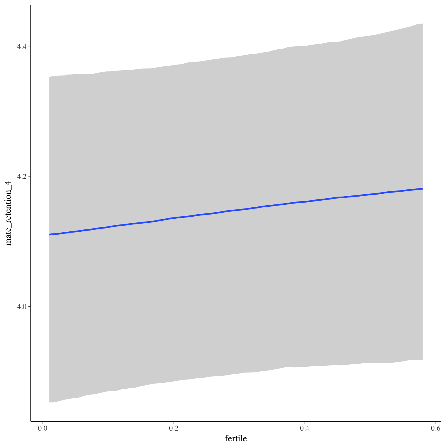
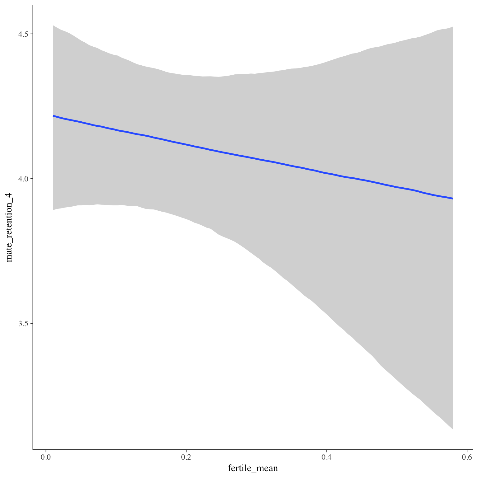
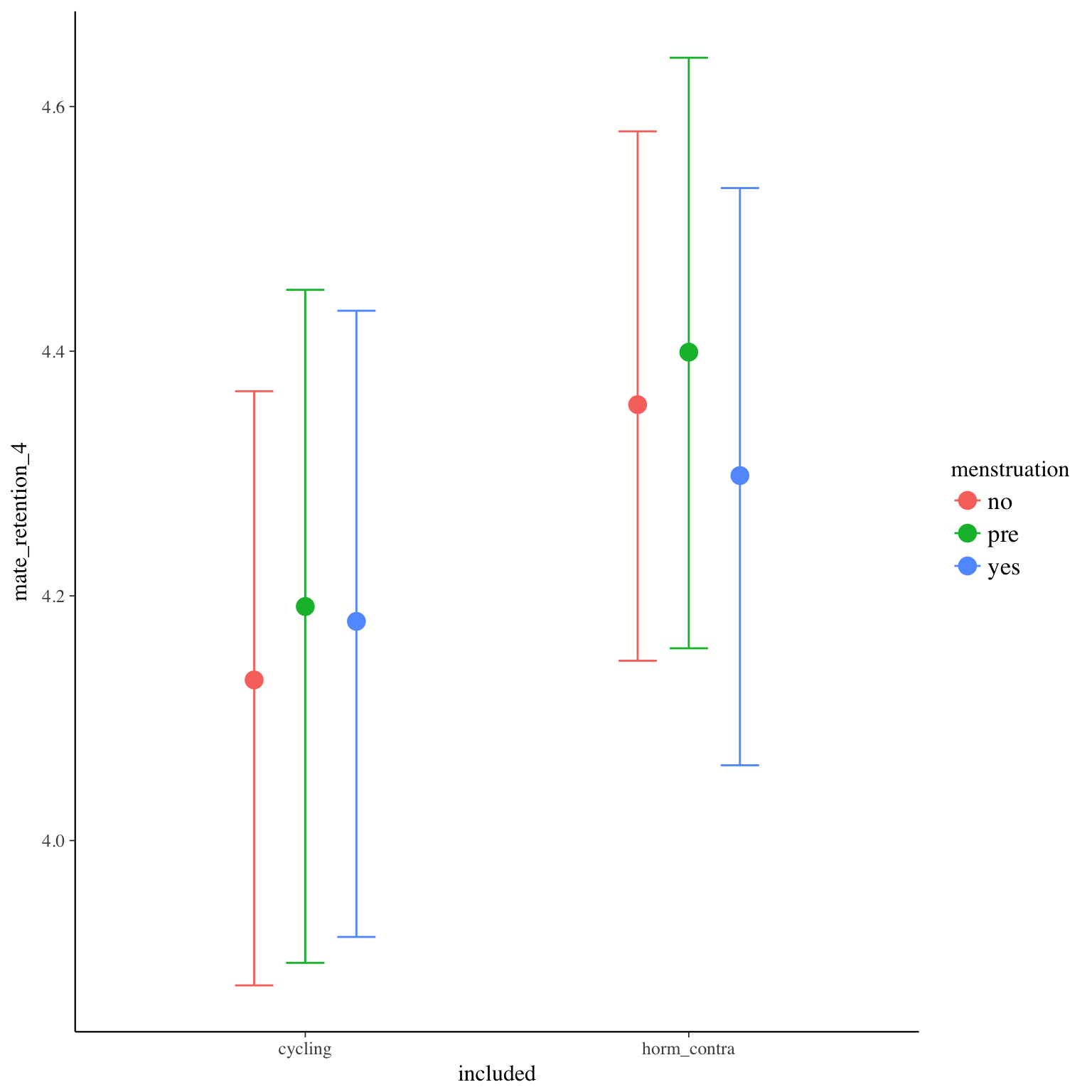
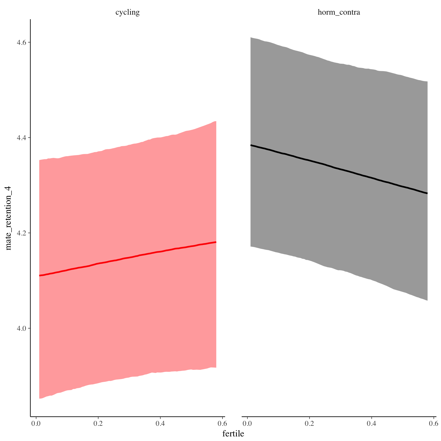
Diagnostics
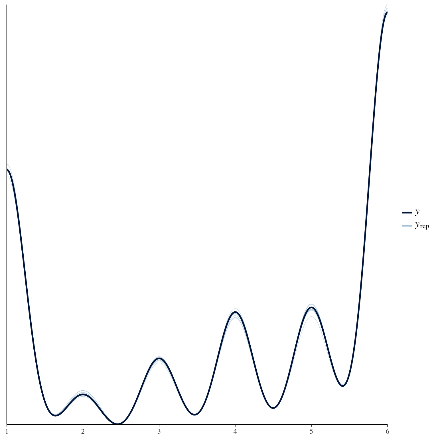
mate_retention_5
Item text:
… habe ich vor meinem Partner über andere Frauen gelästert.
Item translation:
Choices:
| choice | value | frequency | percent |
|---|---|---|---|
| 1 | Stimme nicht zu | 22085 | 0.74 |
| 2 | Stimme überwiegend nicht zu | 2475 | 0.08 |
| 3 | Stimme eher nicht zu | 1817 | 0.06 |
| 4 | Stimme eher zu | 2071 | 0.07 |
| 5 | Stimme überwiegend zu | 824 | 0.03 |
| 6 | Stimme voll zu | 604 | 0.02 |
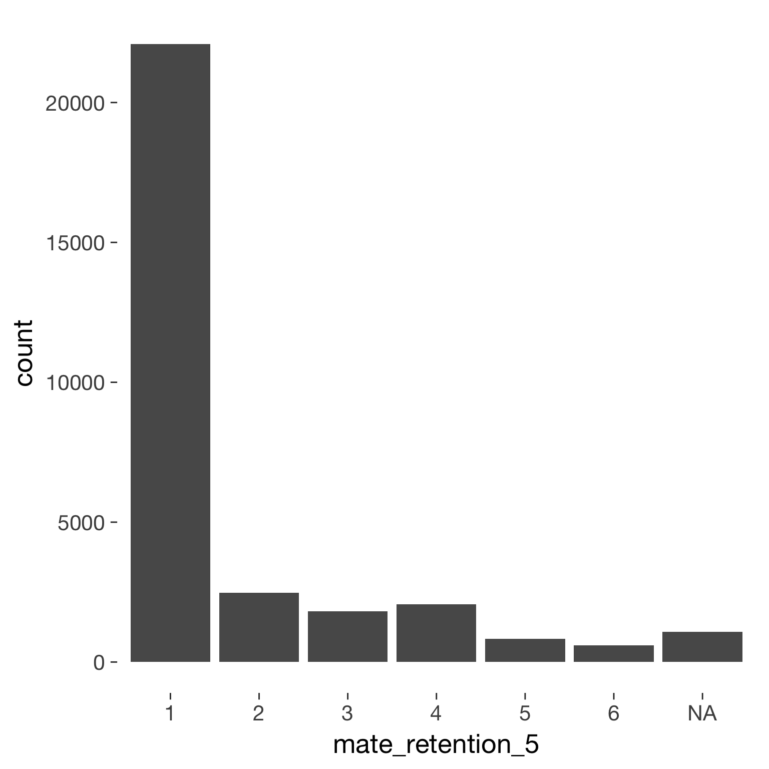
Model
Model summary
 Family: cumulative(logit)
Formula: mate_retention_5 ~ included * (menstruation + fertile) + fertile_mean + (1 + fertile + menstruation | person)
         disc = 1
   Data: diary (Number of observations: 26545)
Samples: 4 chains, each with iter = 2000; warmup = 1000; thin = 1;
         total post-warmup samples = 4000
    ICs: LOO = 44539.06; WAIC = Not computed

Group-Level Effects:
~person (Number of levels: 1043)
                                     Estimate Est.Error l-95% CI u-95% CI Eff.Sample Rhat
sd(Intercept)                            1.57      0.06     1.46     1.69       1368 1.00
sd(fertile)                              1.37      0.19     0.98     1.73        415 1.00
sd(menstruationpre)                      0.55      0.13     0.17     0.76         91 1.04
sd(menstruationyes)                      0.78      0.09     0.61     0.94        537 1.00
cor(Intercept,fertile)                  -0.09      0.11    -0.30     0.14       2121 1.00
cor(Intercept,menstruationpre)           0.02      0.16    -0.26     0.39        241 1.02
cor(fertile,menstruationpre)             0.32      0.21    -0.17     0.66        238 1.01
cor(Intercept,menstruationyes)          -0.10      0.10    -0.29     0.10       1536 1.00
cor(fertile,menstruationyes)             0.12      0.16    -0.23     0.41        395 1.01
cor(menstruationpre,menstruationyes)     0.07      0.23    -0.58     0.43        125 1.04

Population-Level Effects:
                                    Estimate Est.Error l-95% CI u-95% CI Eff.Sample Rhat
Intercept[1]                            1.53      0.14     1.27     1.80       1800    1
Intercept[2]                            2.21      0.14     1.94     2.48       1806    1
Intercept[3]                            2.83      0.14     2.56     3.11       1831    1
Intercept[4]                            3.98      0.14     3.70     4.25       1893    1
Intercept[5]                            4.98      0.15     4.70     5.27       1962    1
includedhorm_contra                     0.15      0.12    -0.08     0.39       1223    1
menstruationpre                        -0.13      0.10    -0.33     0.05       3203    1
menstruationyes                        -0.14      0.10    -0.33     0.06       3056    1
fertile                                -0.18      0.20    -0.56     0.20       2915    1
fertile_mean                            0.43      0.59    -0.67     1.65       2333    1
includedhorm_contra:menstruationpre    -0.05      0.11    -0.26     0.16       4000    1
includedhorm_contra:menstruationyes     0.01      0.11    -0.21     0.24       3093    1
includedhorm_contra:fertile            -0.15      0.22    -0.60     0.26       2861    1

Samples were drawn using sampling(NUTS). For each parameter, Eff.Sample
is a crude measure of effective sample size, and Rhat is the potential
scale reduction factor on split chains (at convergence, Rhat = 1).
Coefficient plot

Marginal effect plots
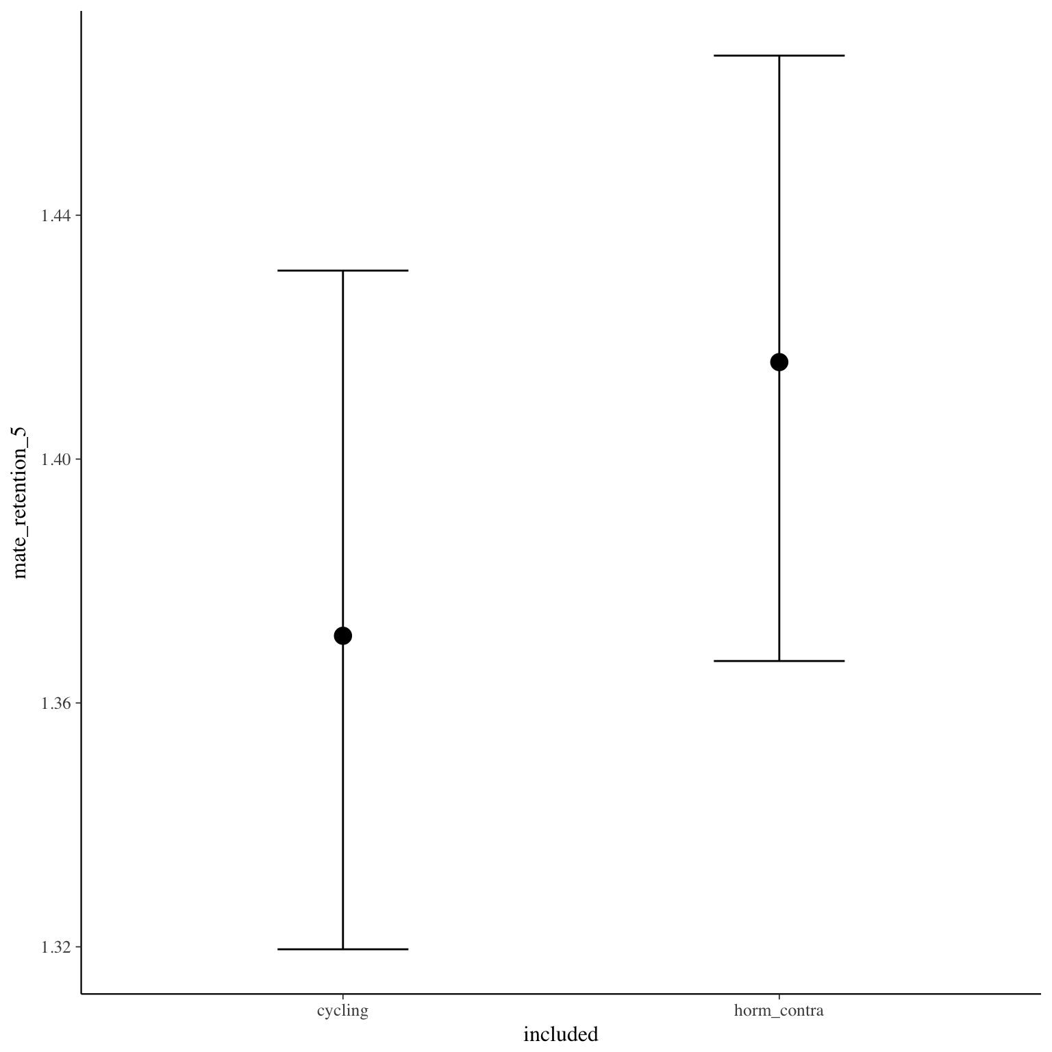
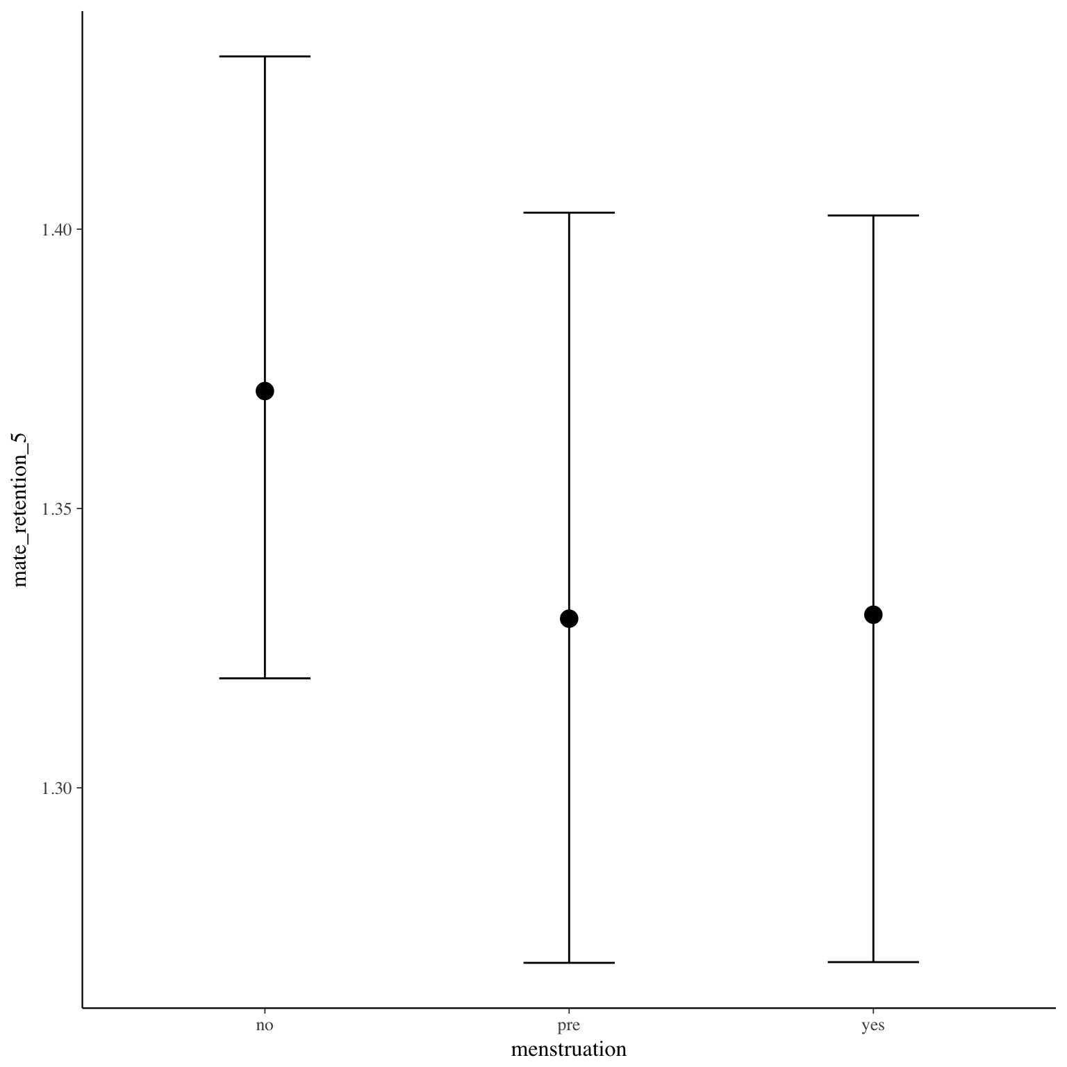
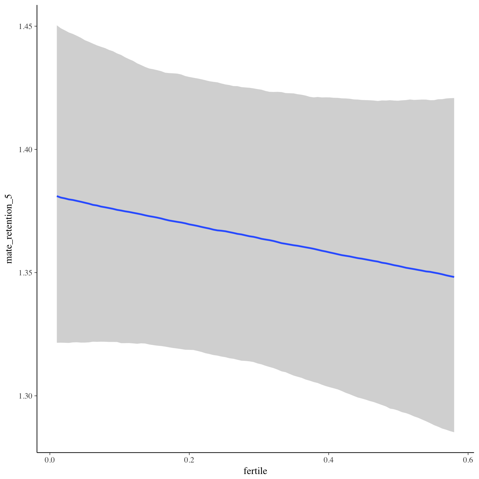
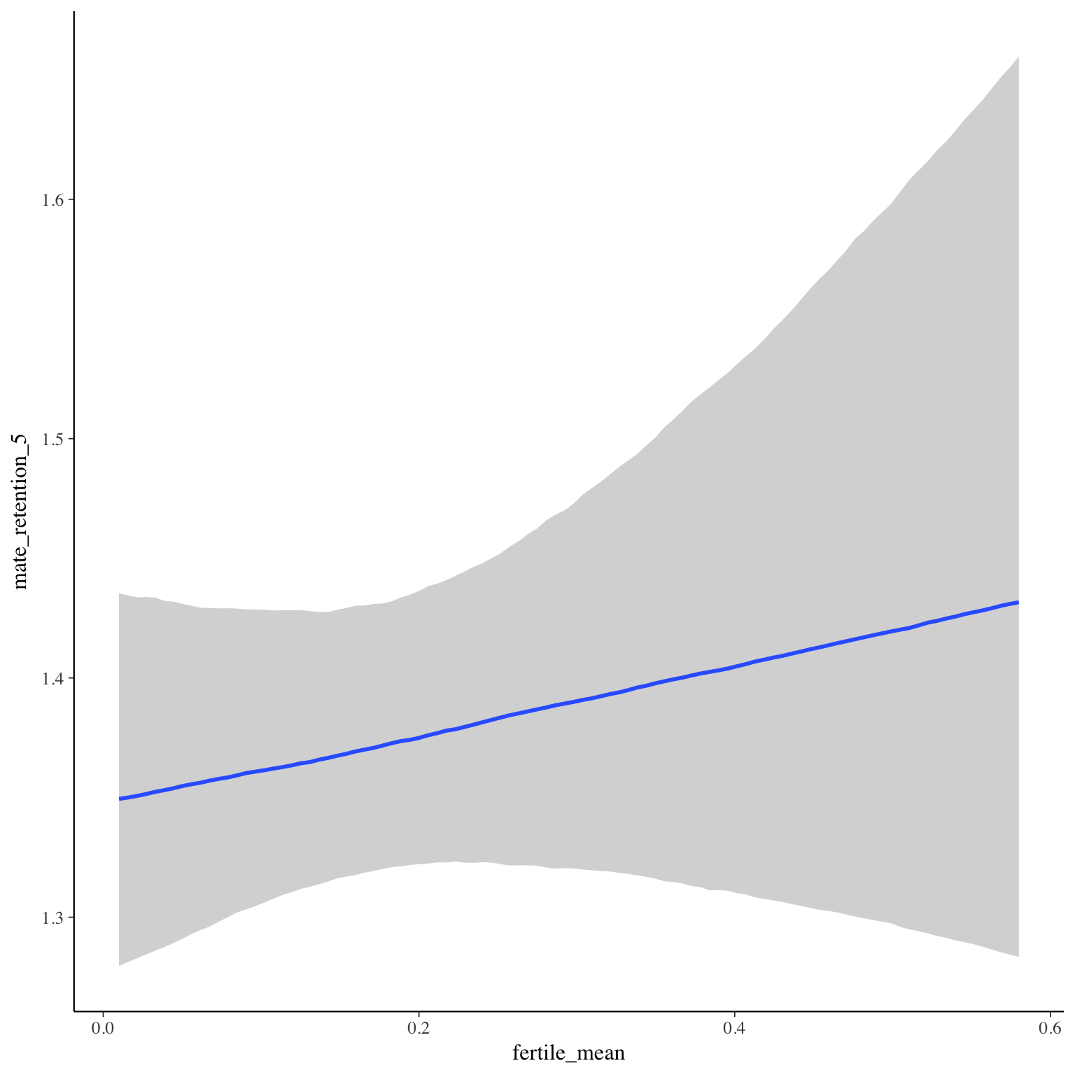
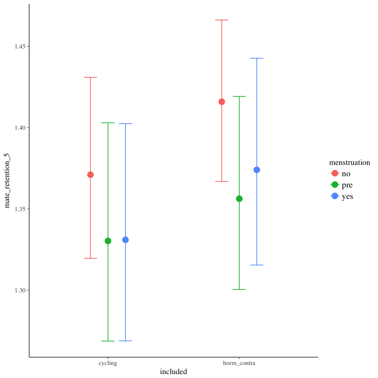
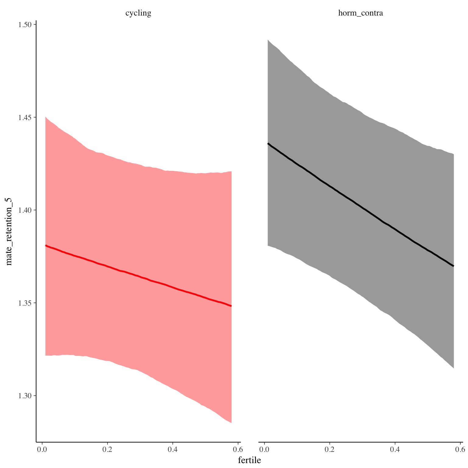
Diagnostics
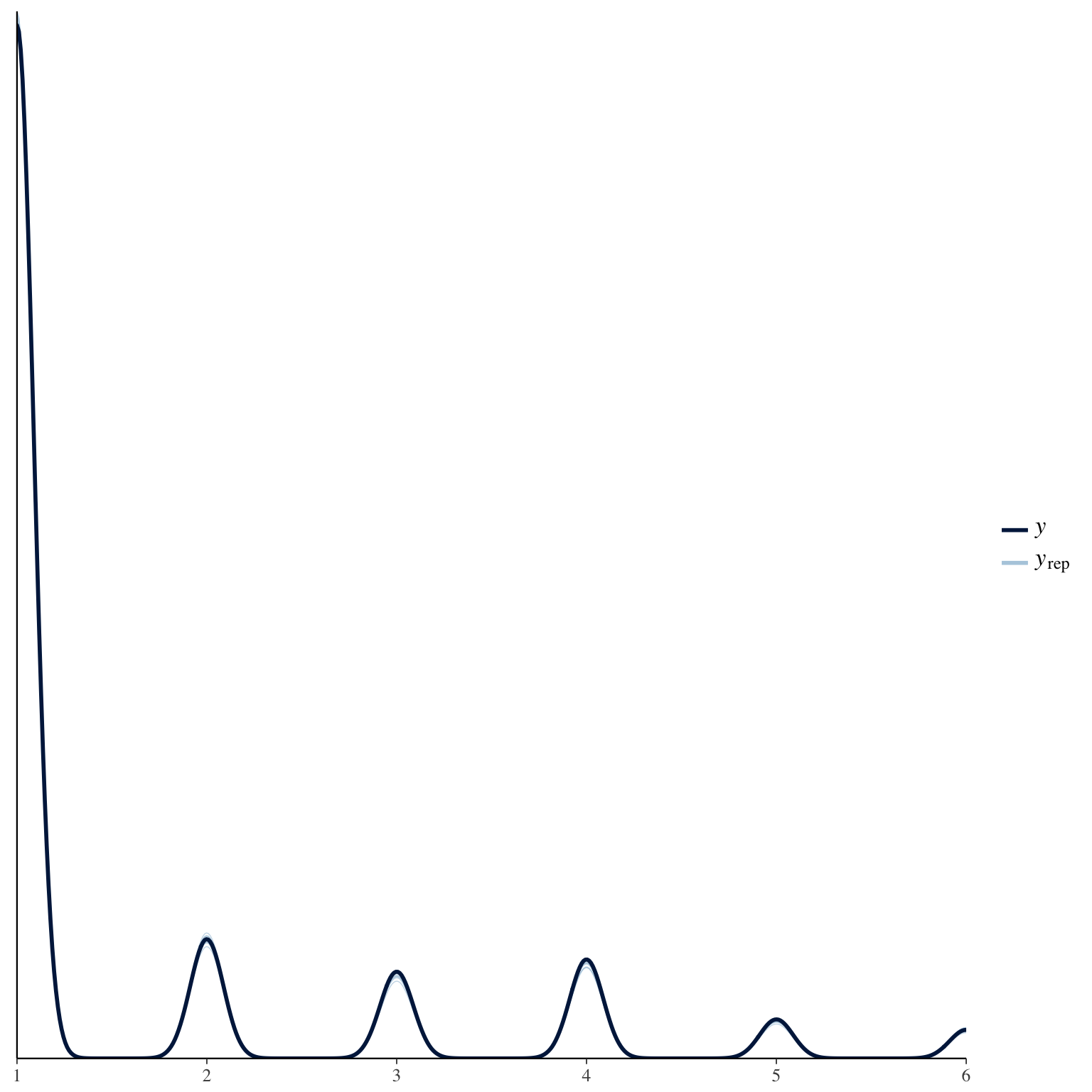
mate_retention_6
Item text:
… war ich in Bezug auf meinen Partner sehr anhänglich.
Item translation:
40. I was very attached to my partner.
Choices:
| choice | value | frequency | percent |
|---|---|---|---|
| 1 | Stimme nicht zu | 9646 | 0.32 |
| 2 | Stimme überwiegend nicht zu | 3944 | 0.13 |
| 3 | Stimme eher nicht zu | 5689 | 0.19 |
| 4 | Stimme eher zu | 6026 | 0.2 |
| 5 | Stimme überwiegend zu | 2967 | 0.1 |
| 6 | Stimme voll zu | 1603 | 0.05 |
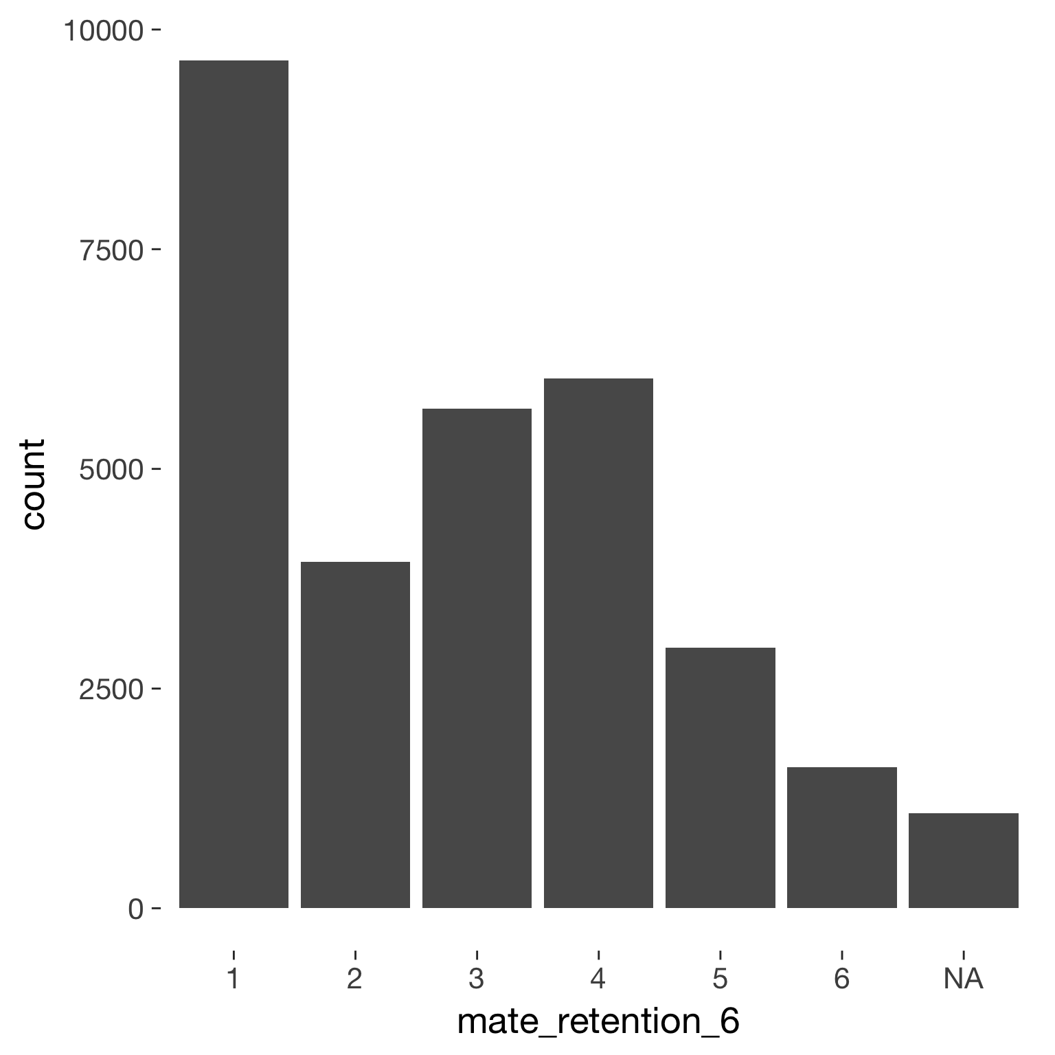
Model
Model summary
 Family: cumulative(logit)
Formula: mate_retention_6 ~ included * (menstruation + fertile) + fertile_mean + (1 + fertile + menstruation | person)
         disc = 1
   Data: diary (Number of observations: 26545)
Samples: 4 chains, each with iter = 2000; warmup = 1000; thin = 1;
         total post-warmup samples = 4000
    ICs: LOO = 74481.1; WAIC = Not computed

Group-Level Effects:
~person (Number of levels: 1043)
                                     Estimate Est.Error l-95% CI u-95% CI Eff.Sample Rhat
sd(Intercept)                            1.72      0.05     1.62     1.82        775 1.01
sd(fertile)                              1.55      0.12     1.30     1.79        463 1.01
sd(menstruationpre)                      0.74      0.06     0.61     0.86        666 1.00
sd(menstruationyes)                      0.77      0.06     0.65     0.89        771 1.01
cor(Intercept,fertile)                  -0.08      0.07    -0.21     0.06       2119 1.00
cor(Intercept,menstruationpre)          -0.02      0.08    -0.17     0.13       1992 1.00
cor(fertile,menstruationpre)             0.33      0.09     0.13     0.50        609 1.00
cor(Intercept,menstruationyes)          -0.10      0.07    -0.23     0.04       1979 1.00
cor(fertile,menstruationyes)             0.24      0.10     0.04     0.42        519 1.00
cor(menstruationpre,menstruationyes)     0.53      0.09     0.34     0.69        438 1.01

Population-Level Effects:
                                    Estimate Est.Error l-95% CI u-95% CI Eff.Sample Rhat
Intercept[1]                           -1.00      0.14    -1.28    -0.74        494 1.01
Intercept[2]                           -0.14      0.14    -0.42     0.12        489 1.01
Intercept[3]                            1.02      0.14     0.73     1.28        517 1.01
Intercept[4]                            2.59      0.14     2.31     2.86        519 1.01
Intercept[5]                            4.12      0.14     3.84     4.39        537 1.01
includedhorm_contra                     0.39      0.12     0.15     0.62        374 1.00
menstruationpre                        -0.05      0.07    -0.20     0.09       2052 1.00
menstruationyes                         0.15      0.07     0.01     0.29       1746 1.00
fertile                                -0.05      0.15    -0.35     0.24       1819 1.00
fertile_mean                           -0.49      0.60    -1.69     0.64       1026 1.01
includedhorm_contra:menstruationpre    -0.06      0.09    -0.23     0.13       1826 1.00
includedhorm_contra:menstruationyes    -0.09      0.09    -0.28     0.09       1747 1.00
includedhorm_contra:fertile            -0.35      0.19    -0.72     0.02       1806 1.00

Samples were drawn using sampling(NUTS). For each parameter, Eff.Sample
is a crude measure of effective sample size, and Rhat is the potential
scale reduction factor on split chains (at convergence, Rhat = 1).
Coefficient plot
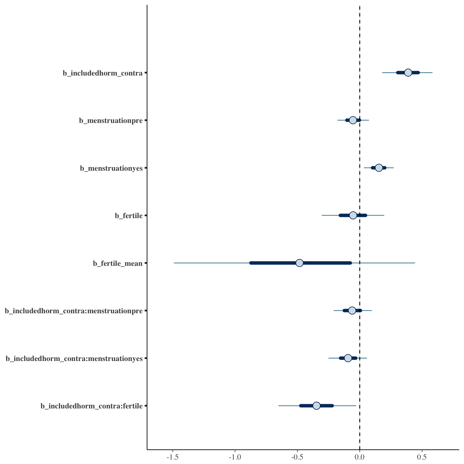
Marginal effect plots
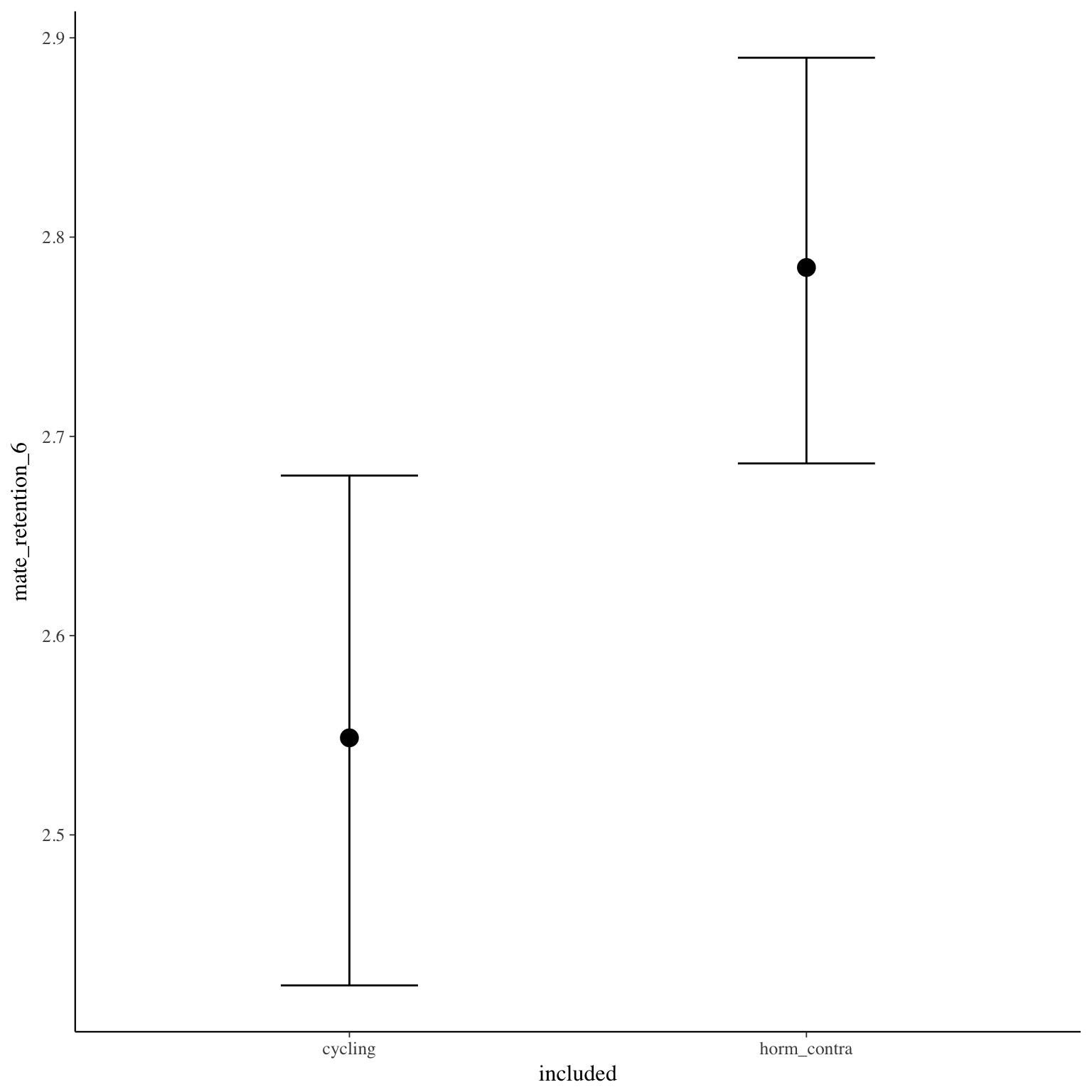
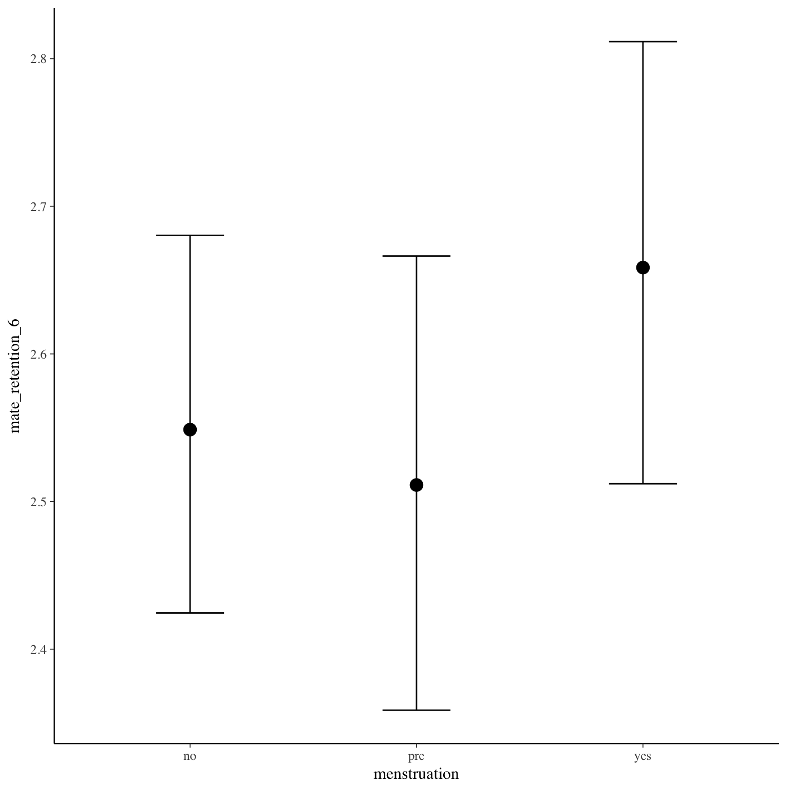
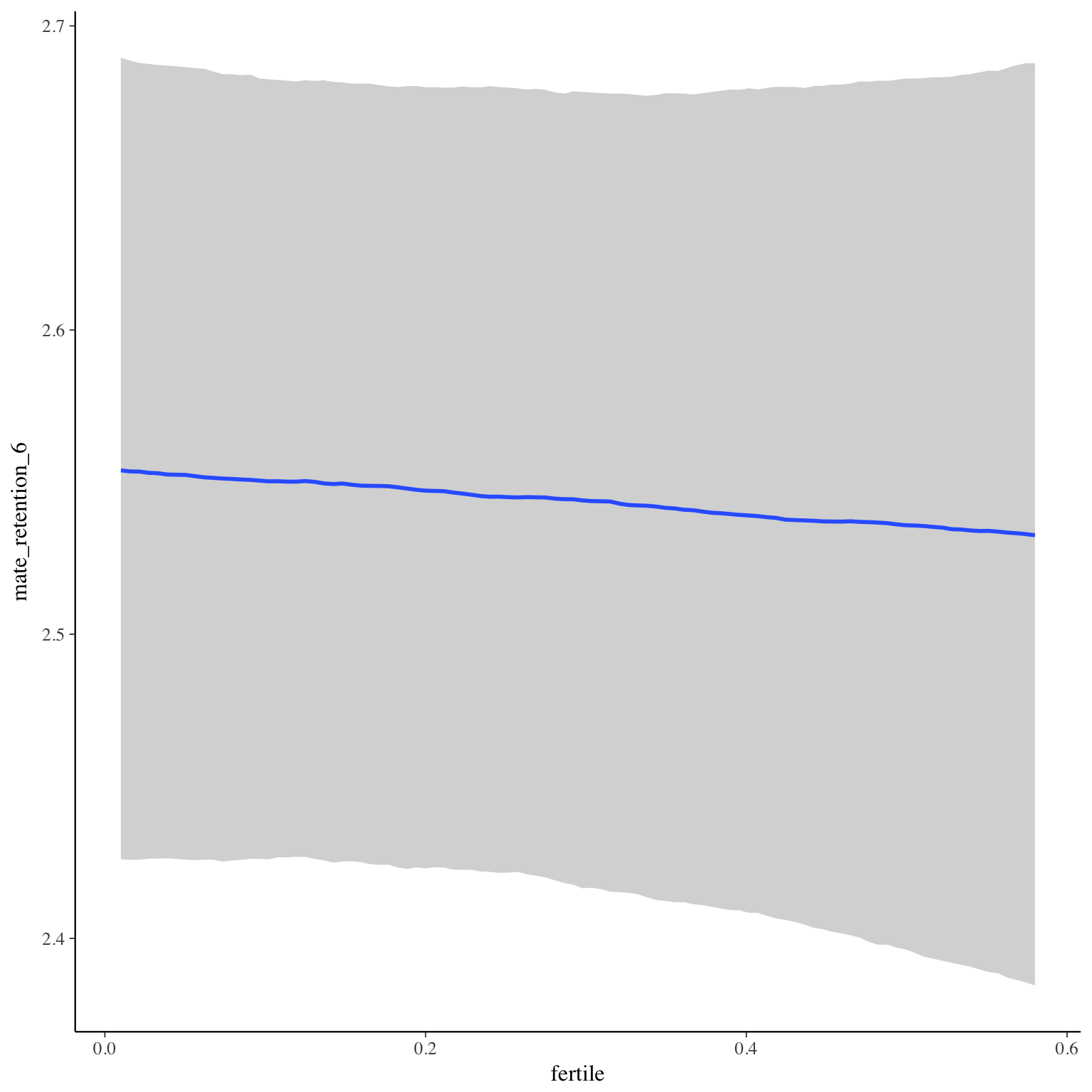
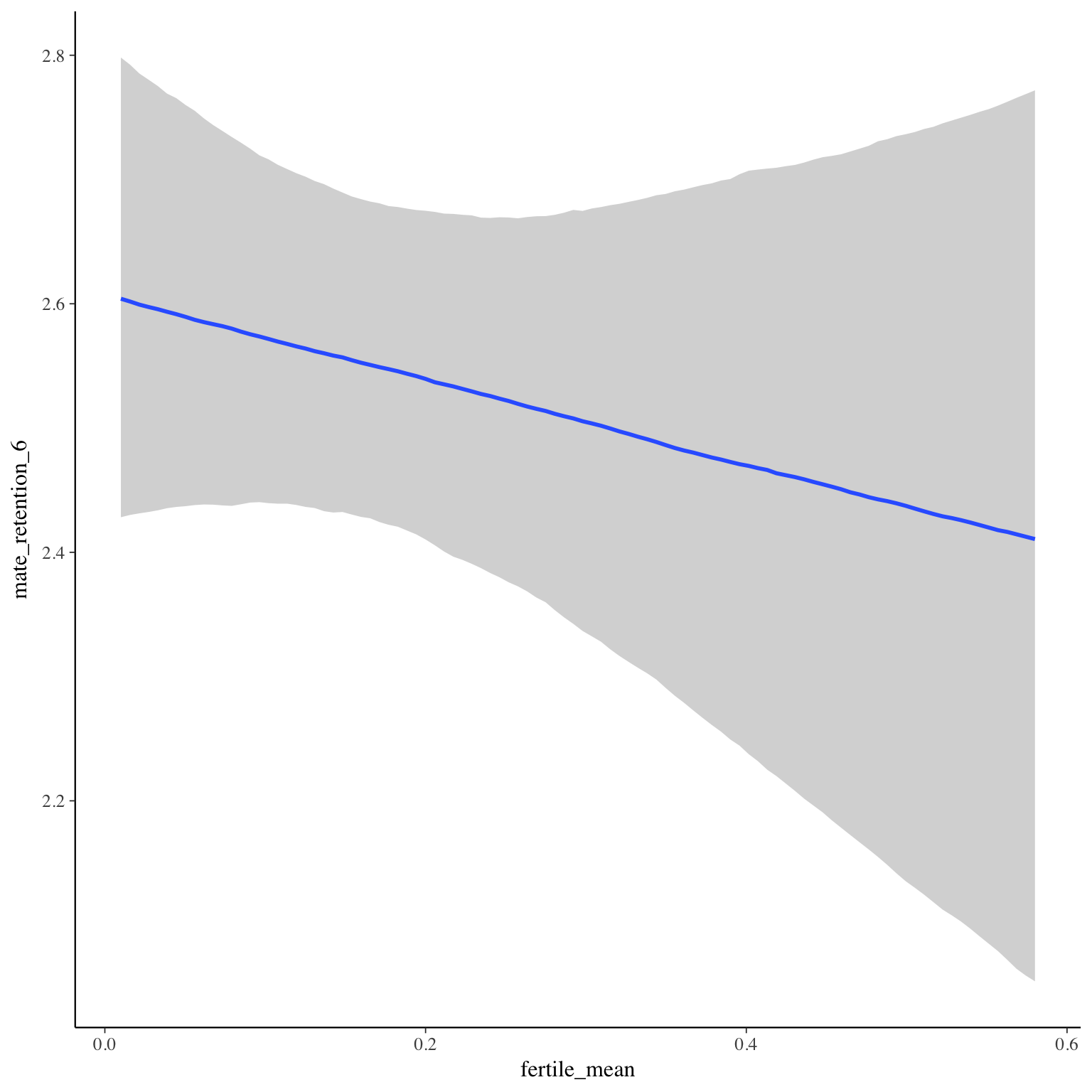
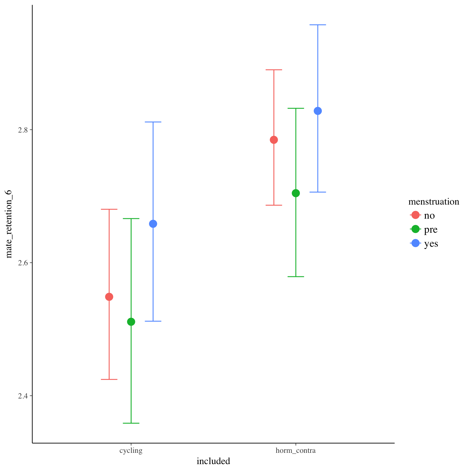
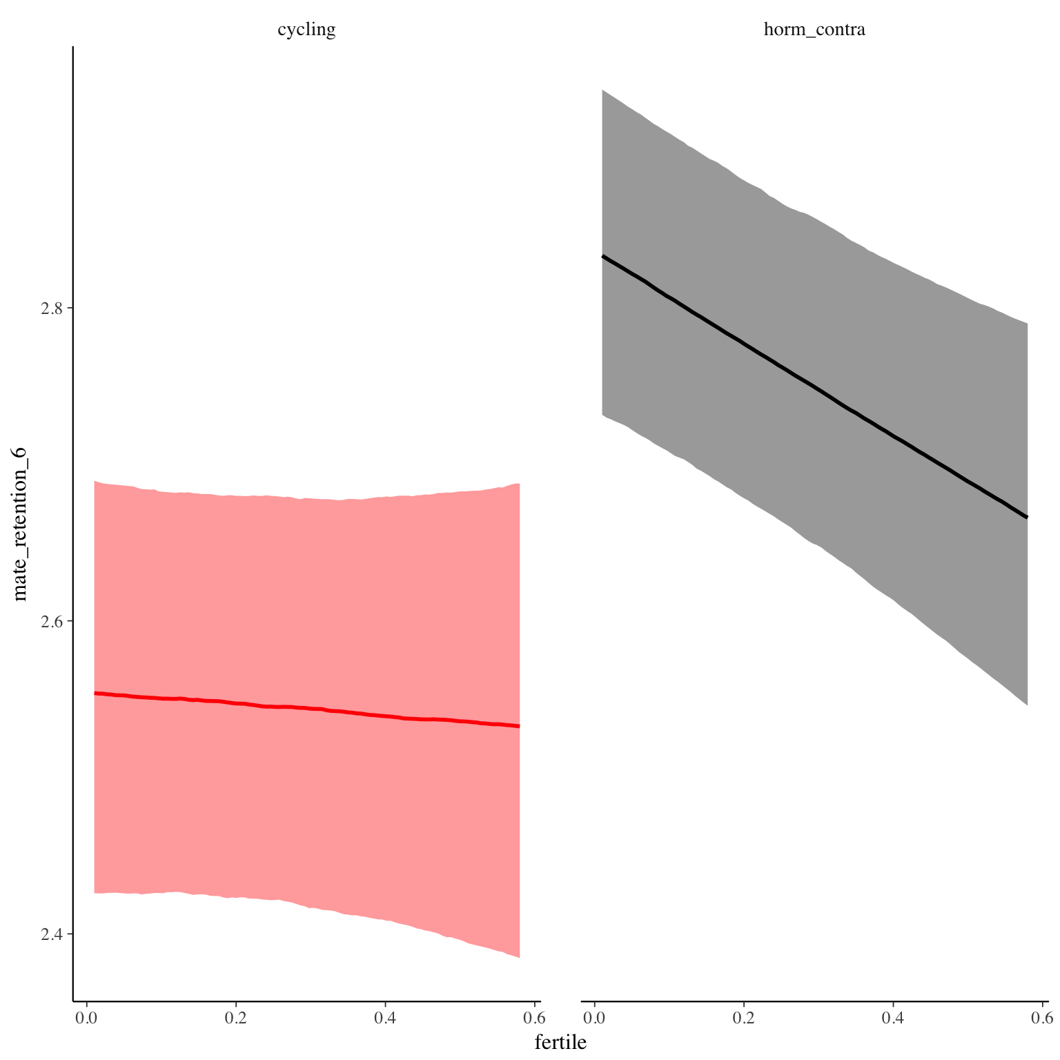
Diagnostics
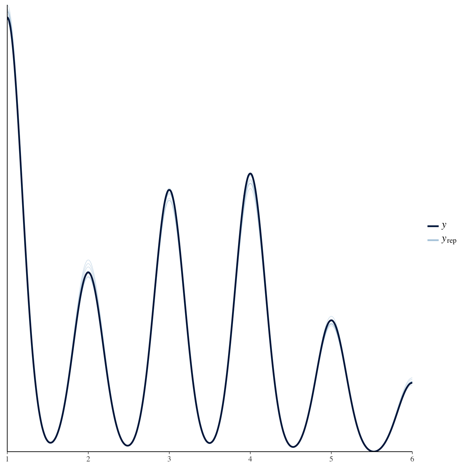
NARQ_admiration_1
Item text:
…hatte ich das Gefühl es verdient zu haben, als große Persönlichkeit angesehen zu werden.
Item translation:
27. I deserved to be seen as a great personality.
Choices:
| choice | value | frequency | percent |
|---|---|---|---|
| 1 | Stimme nicht zu | 10545 | 0.35 |
| 2 | Stimme überwiegend nicht zu | 4120 | 0.14 |
| 3 | Stimme eher nicht zu | 6077 | 0.2 |
| 4 | Stimme eher zu | 6020 | 0.2 |
| 5 | Stimme überwiegend zu | 2289 | 0.08 |
| 6 | Stimme voll zu | 826 | 0.03 |
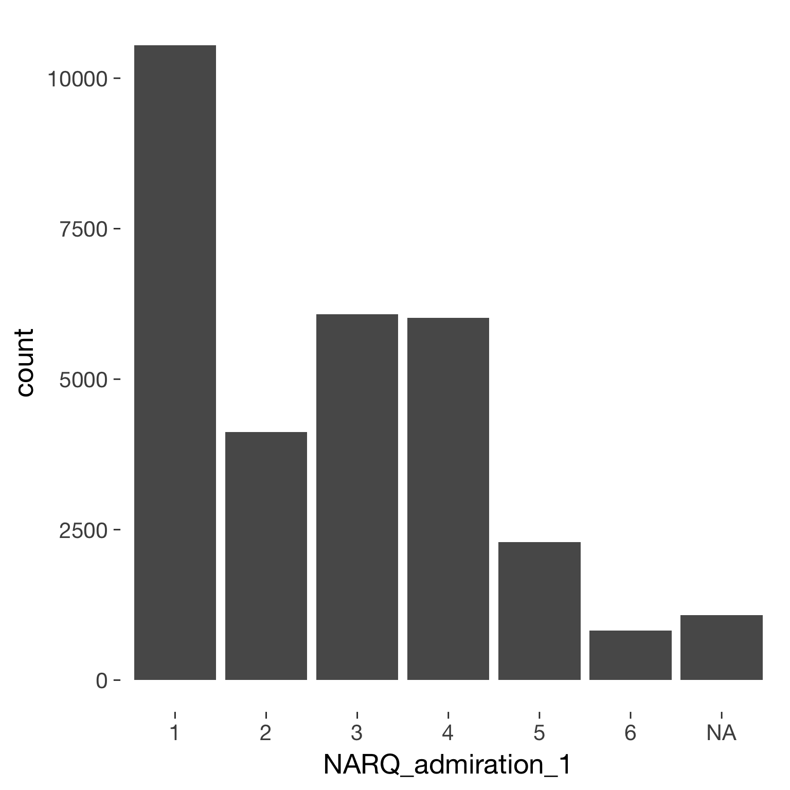
Model
Model summary
 Family: cumulative(logit)
Formula: NARQ_admiration_1 ~ included * (menstruation + fertile) + fertile_mean + (1 + fertile + menstruation | person)
         disc = 1
   Data: diary (Number of observations: 26546)
Samples: 4 chains, each with iter = 2000; warmup = 1000; thin = 1;
         total post-warmup samples = 4000
    ICs: LOO = 54982.3; WAIC = Not computed

Group-Level Effects:
~person (Number of levels: 1043)
                                     Estimate Est.Error l-95% CI u-95% CI Eff.Sample Rhat
sd(Intercept)                            3.30      0.09     3.13     3.48        443 1.01
sd(fertile)                              1.81      0.13     1.56     2.07        580 1.00
sd(menstruationpre)                      0.64      0.07     0.49     0.78        438 1.01
sd(menstruationyes)                      0.78      0.06     0.65     0.90        515 1.01
cor(Intercept,fertile)                  -0.11      0.08    -0.26     0.03       2161 1.00
cor(Intercept,menstruationpre)          -0.18      0.10    -0.37     0.01       2096 1.00
cor(fertile,menstruationpre)             0.10      0.12    -0.17     0.32        387 1.01
cor(Intercept,menstruationyes)          -0.27      0.08    -0.43    -0.11       1883 1.00
cor(fertile,menstruationyes)             0.16      0.11    -0.06     0.36        365 1.00
cor(menstruationpre,menstruationyes)     0.54      0.11     0.31     0.75        282 1.01

Population-Level Effects:
                                    Estimate Est.Error l-95% CI u-95% CI Eff.Sample Rhat
Intercept[1]                           -1.32      0.24    -1.76    -0.84        121 1.04
Intercept[2]                            0.16      0.24    -0.29     0.64        121 1.04
Intercept[3]                            2.11      0.24     1.66     2.60        121 1.04
Intercept[4]                            4.55      0.24     4.10     5.04        122 1.04
Intercept[5]                            6.70      0.24     6.25     7.20        125 1.04
includedhorm_contra                    -0.30      0.23    -0.73     0.14         77 1.06
menstruationpre                        -0.04      0.08    -0.19     0.11       1690 1.00
menstruationyes                        -0.18      0.08    -0.34    -0.03       1509 1.00
fertile                                 0.10      0.17    -0.24     0.44       1418 1.00
fertile_mean                            0.72      0.90    -0.91     2.67        532 1.00
includedhorm_contra:menstruationpre     0.04      0.10    -0.14     0.23       1714 1.00
includedhorm_contra:menstruationyes     0.17      0.10    -0.03     0.38       1435 1.00
includedhorm_contra:fertile            -0.24      0.22    -0.68     0.17       1482 1.00

Samples were drawn using sampling(NUTS). For each parameter, Eff.Sample
is a crude measure of effective sample size, and Rhat is the potential
scale reduction factor on split chains (at convergence, Rhat = 1).
Coefficient plot
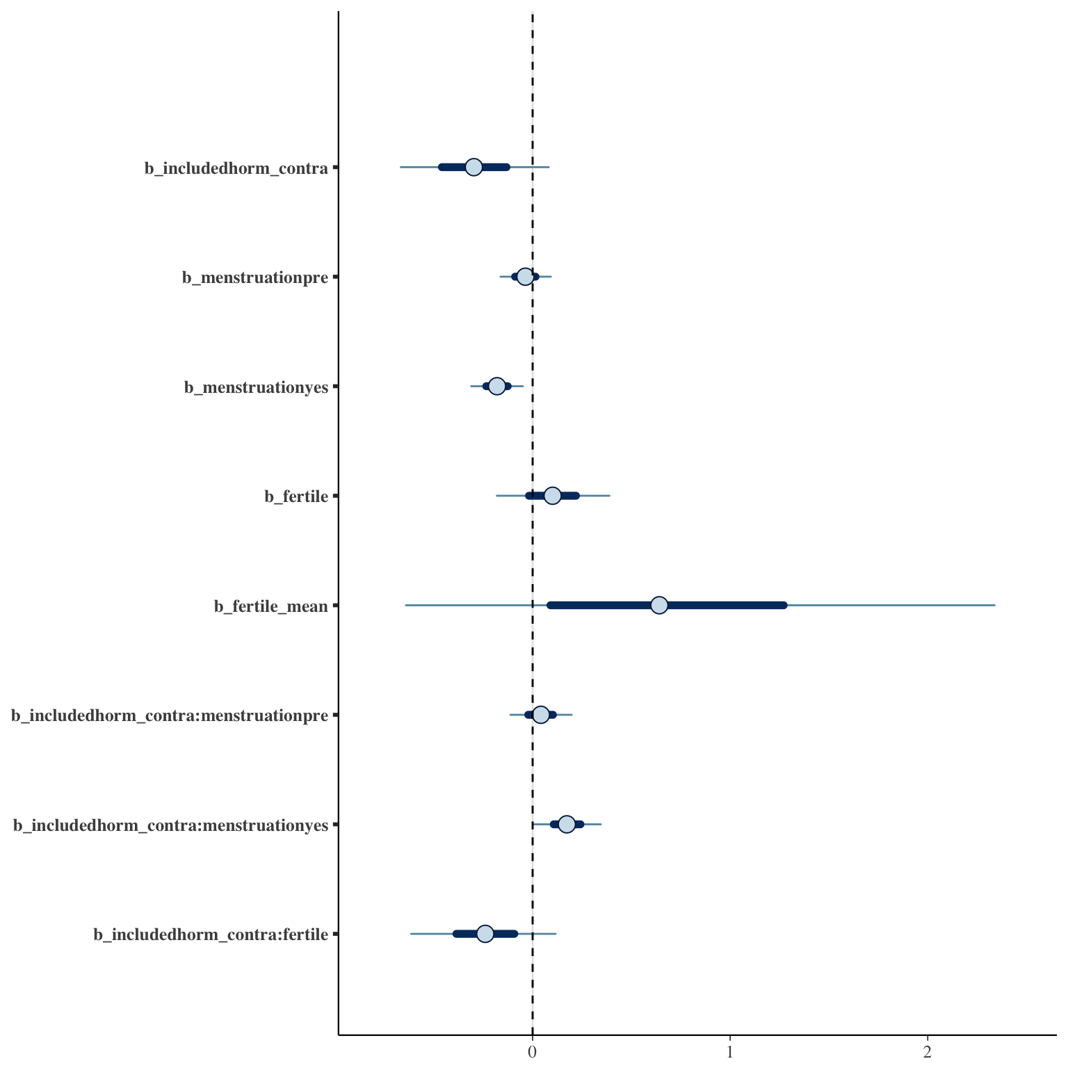
Marginal effect plots
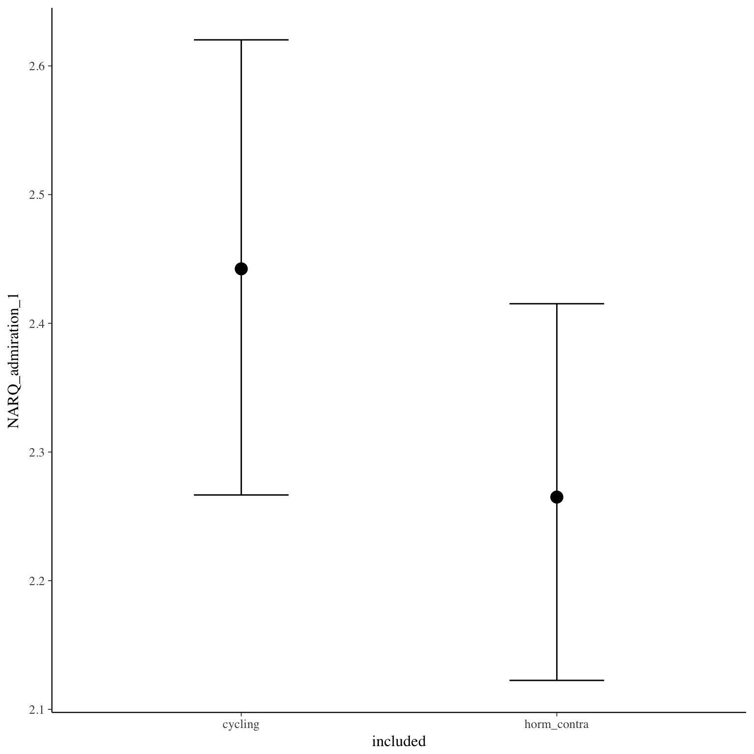
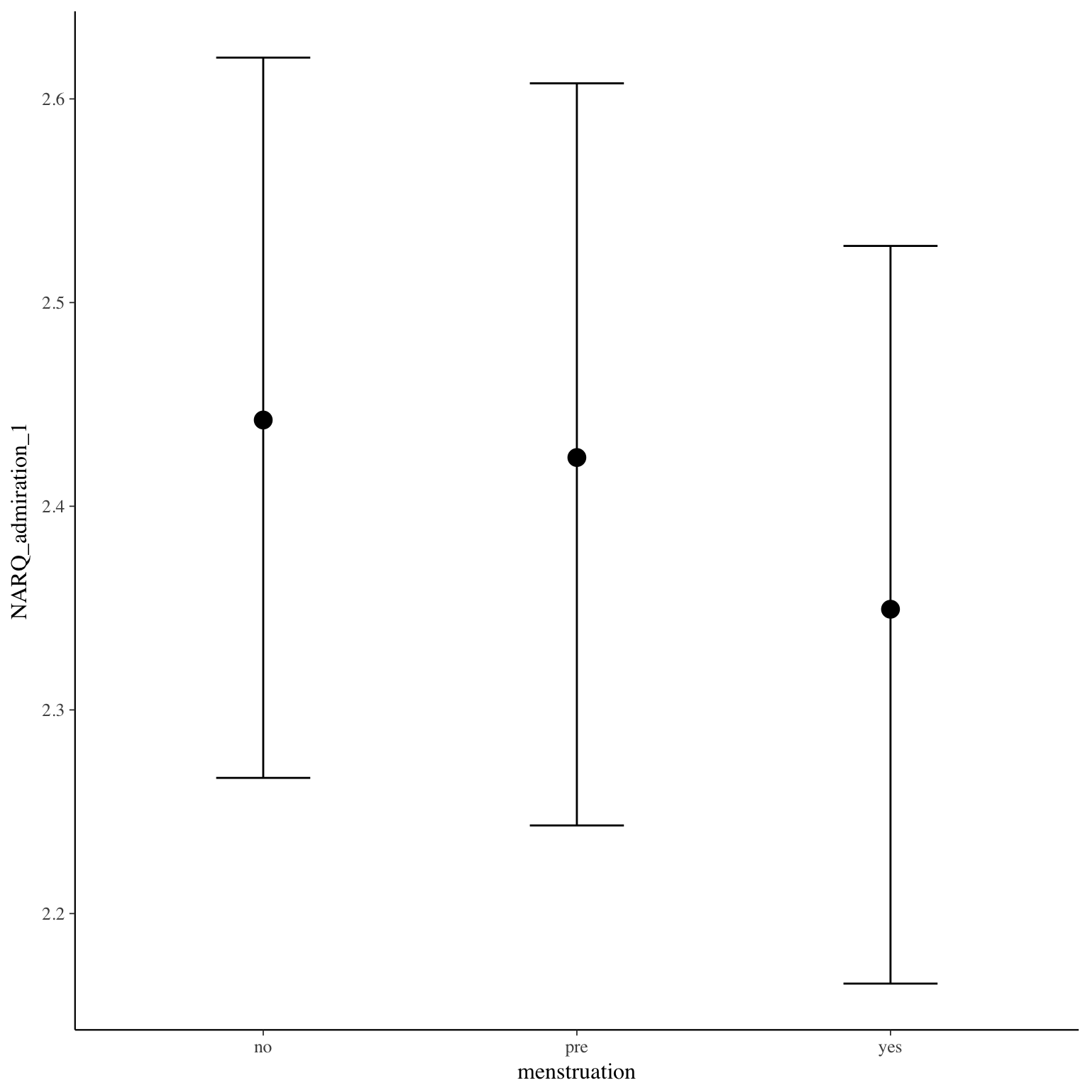
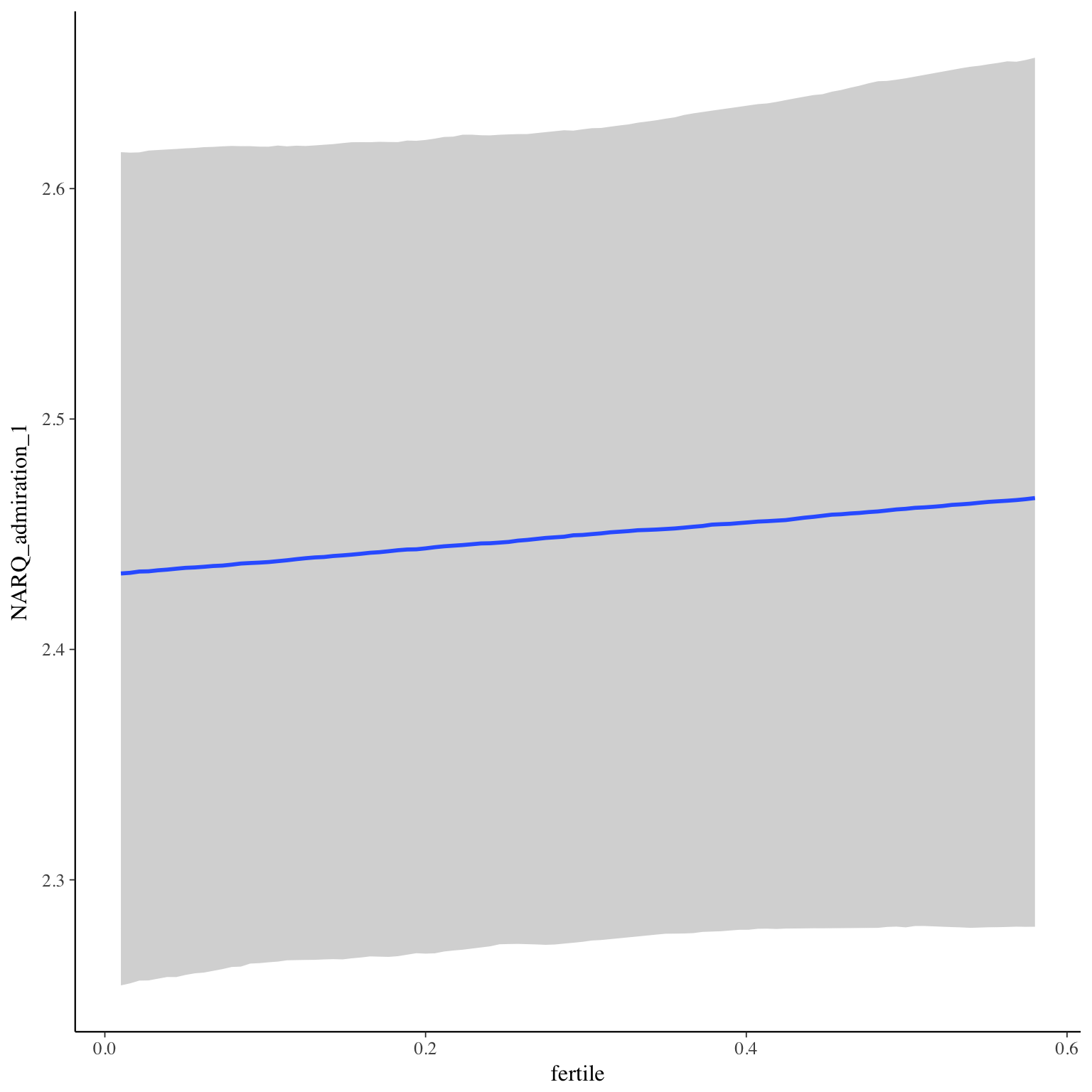
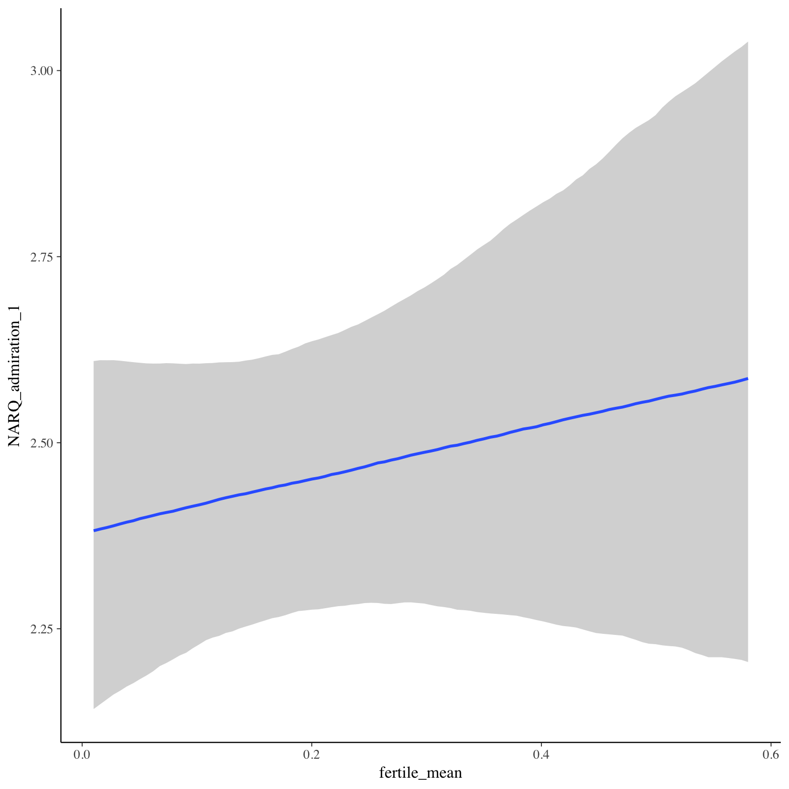
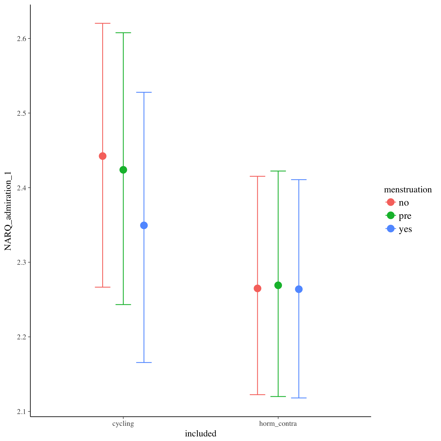
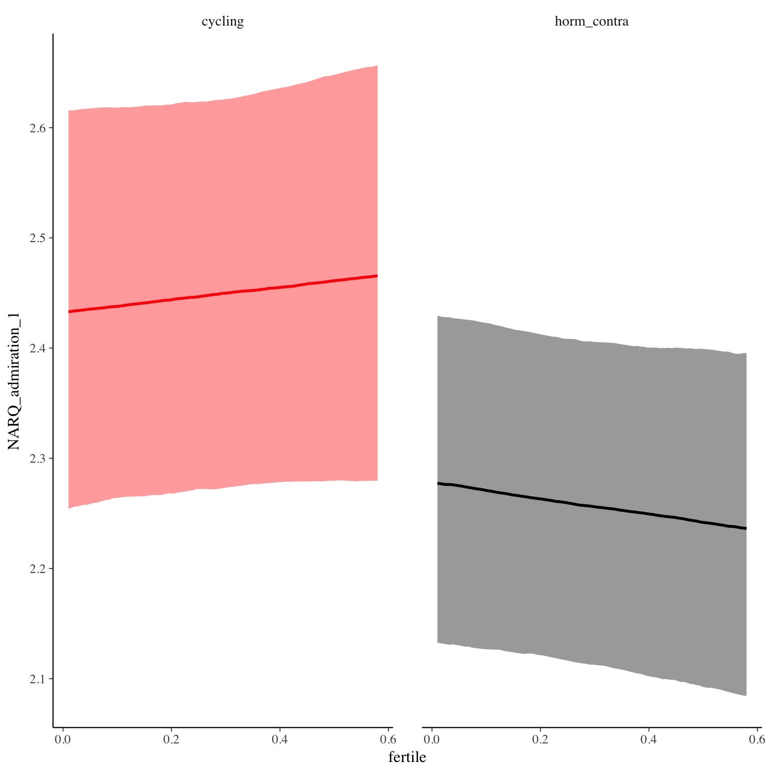
Diagnostics
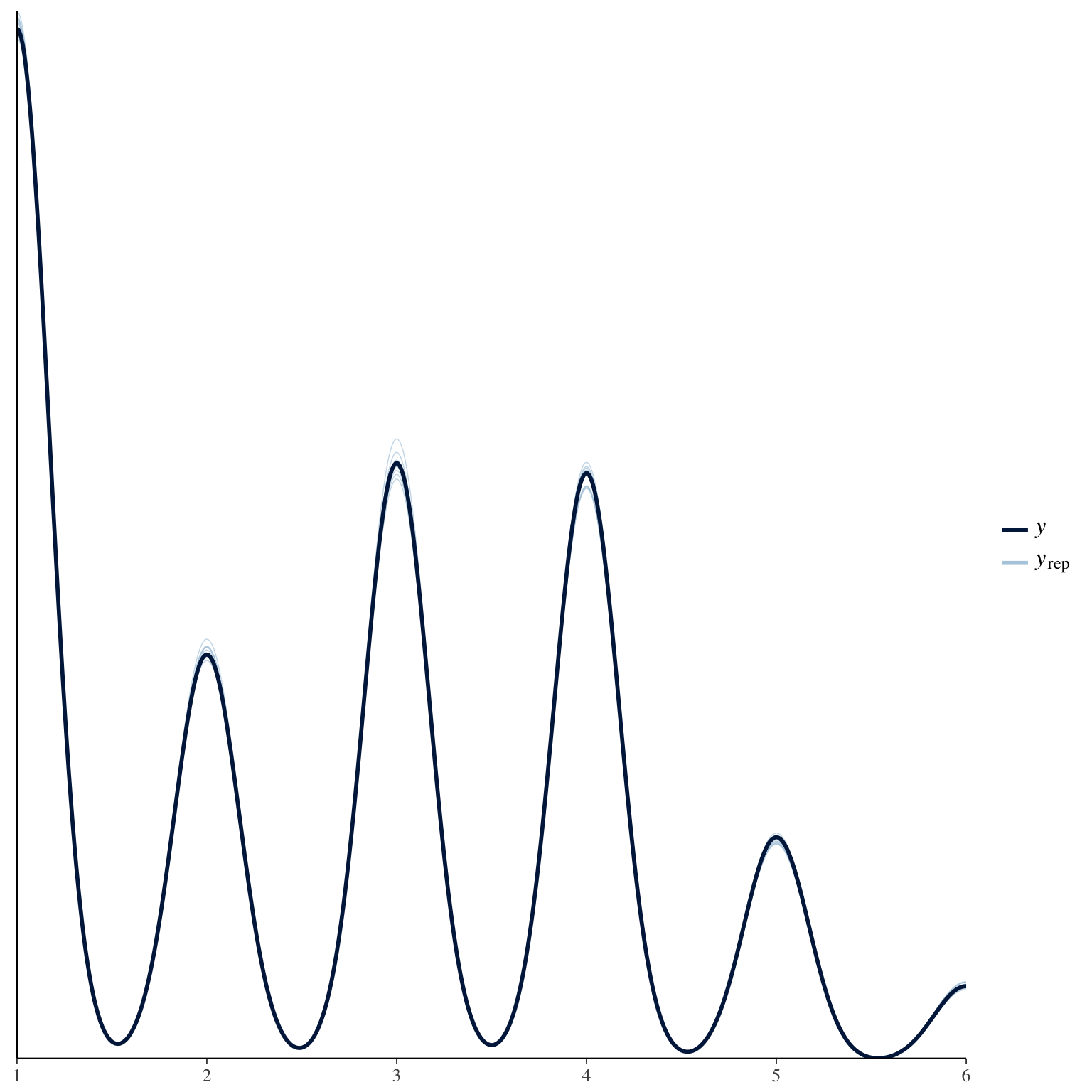
NARQ_admiration_2
Item text:
… habe ich viel Kraft daraus gezogen, eine ganz besondere Person zu sein.
Item translation:
28. Being a very special person gave me a lot of strength.
Choices:
| choice | value | frequency | percent |
|---|---|---|---|
| 1 | Stimme nicht zu | 10803 | 0.36 |
| 2 | Stimme überwiegend nicht zu | 3991 | 0.13 |
| 3 | Stimme eher nicht zu | 5827 | 0.2 |
| 4 | Stimme eher zu | 6000 | 0.2 |
| 5 | Stimme überwiegend zu | 2397 | 0.08 |
| 6 | Stimme voll zu | 859 | 0.03 |
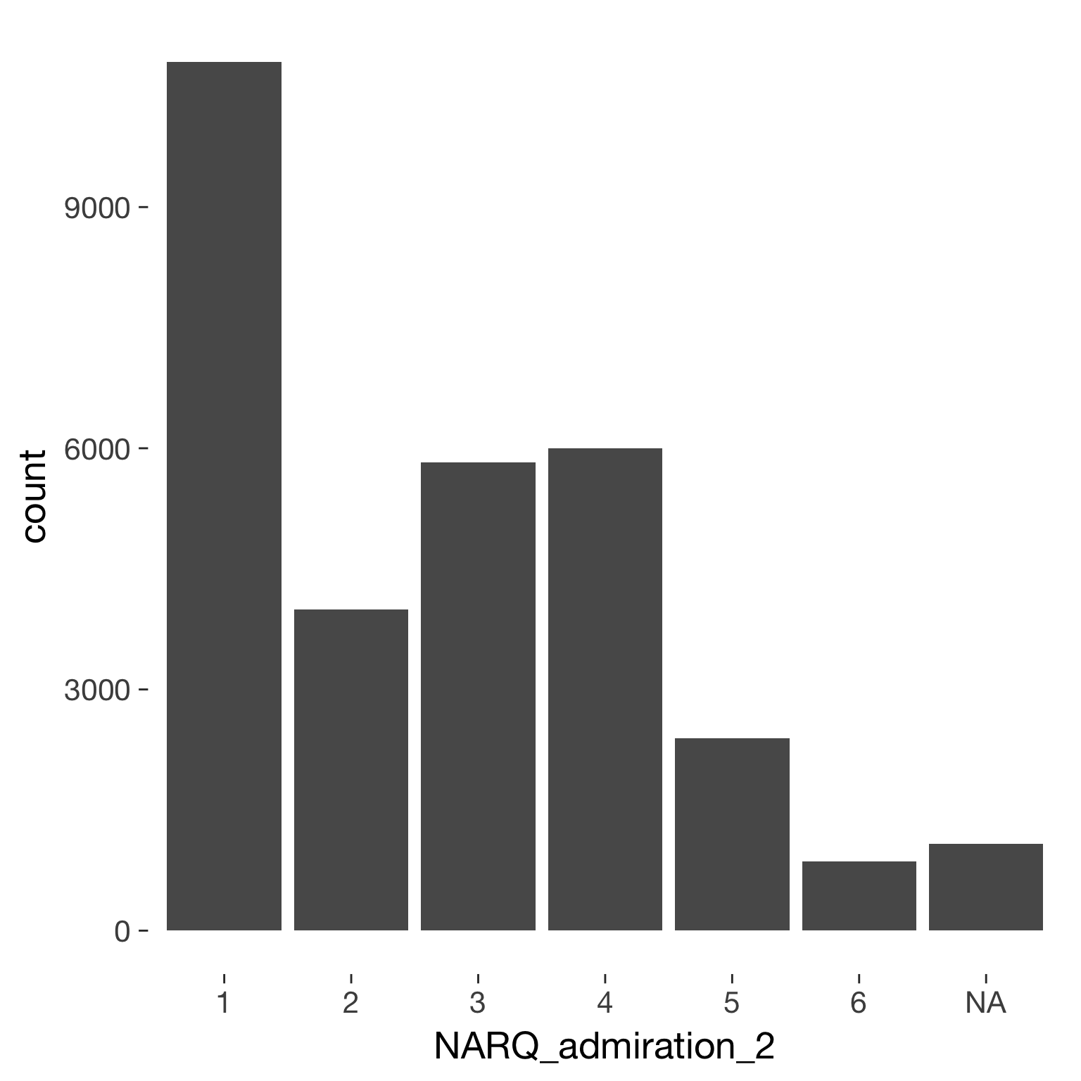
Model
Model summary
 Family: cumulative(logit)
Formula: NARQ_admiration_2 ~ included * (menstruation + fertile) + fertile_mean + (1 + fertile + menstruation | person)
         disc = 1
   Data: diary (Number of observations: 26546)
Samples: 4 chains, each with iter = 2000; warmup = 1000; thin = 1;
         total post-warmup samples = 4000
    ICs: LOO = 56131.73; WAIC = Not computed

Group-Level Effects:
~person (Number of levels: 1043)
                                     Estimate Est.Error l-95% CI u-95% CI Eff.Sample Rhat
sd(Intercept)                            3.20      0.09     3.04     3.39        490 1.00
sd(fertile)                              1.75      0.13     1.49     2.02        523 1.01
sd(menstruationpre)                      0.64      0.08     0.47     0.79        363 1.01
sd(menstruationyes)                      0.81      0.06     0.68     0.93        708 1.00
cor(Intercept,fertile)                  -0.04      0.08    -0.19     0.12       2122 1.00
cor(Intercept,menstruationpre)          -0.25      0.10    -0.43    -0.05       2597 1.00
cor(fertile,menstruationpre)             0.14      0.13    -0.14     0.37        382 1.01
cor(Intercept,menstruationyes)          -0.27      0.08    -0.42    -0.12       2360 1.00
cor(fertile,menstruationyes)             0.21      0.10     0.00     0.39        555 1.00
cor(menstruationpre,menstruationyes)     0.56      0.10     0.36     0.76        329 1.00

Population-Level Effects:
                                    Estimate Est.Error l-95% CI u-95% CI Eff.Sample Rhat
Intercept[1]                           -1.35      0.21    -1.75    -0.93        315 1.01
Intercept[2]                            0.07      0.21    -0.34     0.48        312 1.01
Intercept[3]                            1.87      0.21     1.47     2.28        315 1.01
Intercept[4]                            4.15      0.21     3.74     4.56        321 1.01
Intercept[5]                            6.24      0.21     5.84     6.66        338 1.01
includedhorm_contra                    -0.41      0.20    -0.81    -0.03        178 1.01
menstruationpre                        -0.13      0.08    -0.28     0.02       1846 1.00
menstruationyes                        -0.25      0.08    -0.41    -0.10       2182 1.00
fertile                                -0.15      0.17    -0.49     0.18       1597 1.00
fertile_mean                            0.26      0.77    -1.22     1.82        712 1.01
includedhorm_contra:menstruationpre     0.21      0.10     0.02     0.40       2145 1.00
includedhorm_contra:menstruationyes     0.29      0.10     0.10     0.49       2328 1.00
includedhorm_contra:fertile             0.01      0.20    -0.39     0.42       1724 1.00

Samples were drawn using sampling(NUTS). For each parameter, Eff.Sample
is a crude measure of effective sample size, and Rhat is the potential
scale reduction factor on split chains (at convergence, Rhat = 1).
Coefficient plot
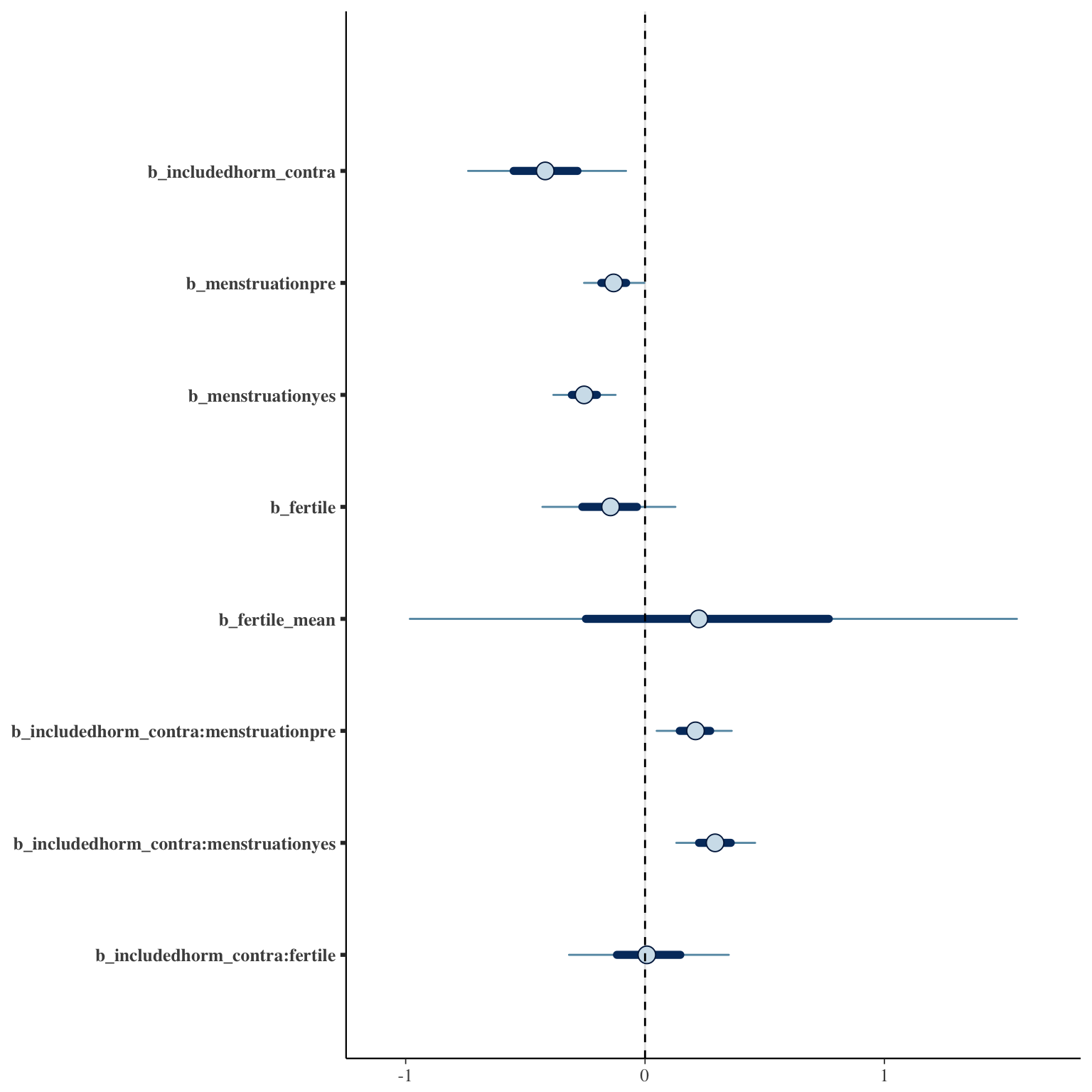
Marginal effect plots
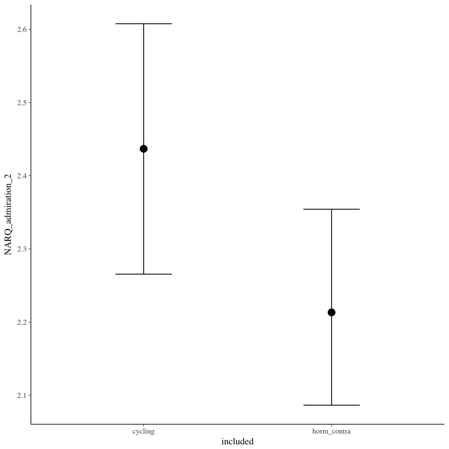
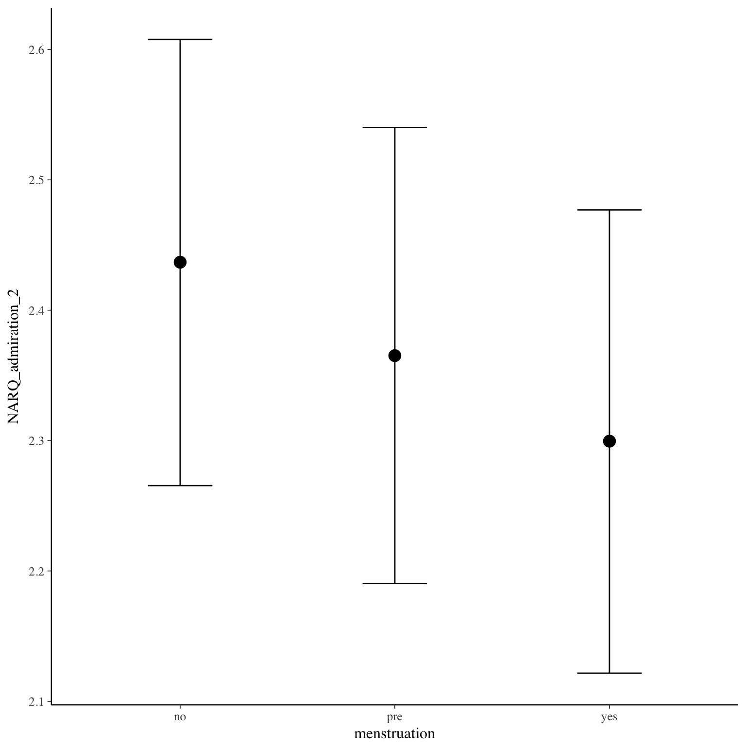
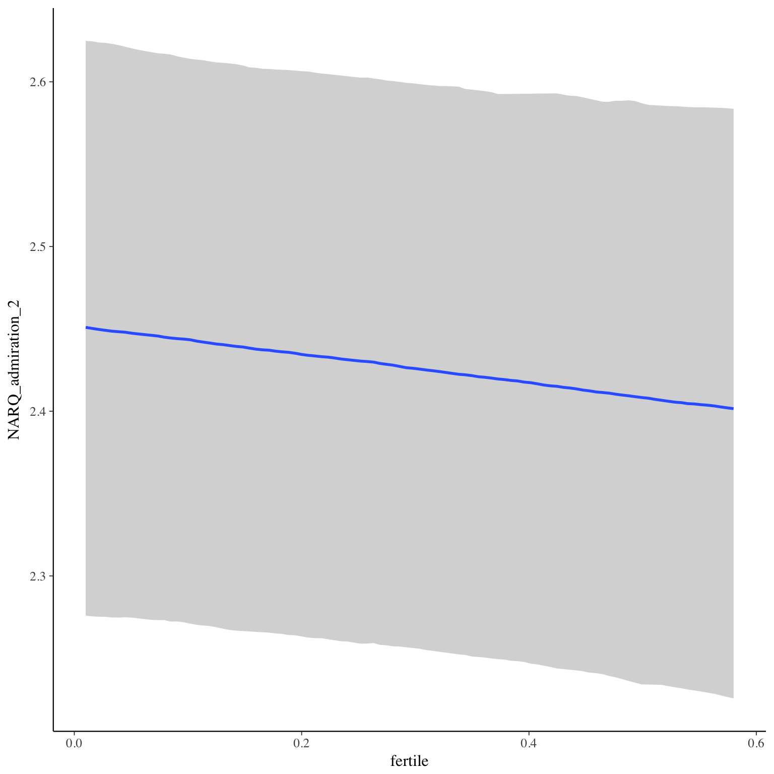
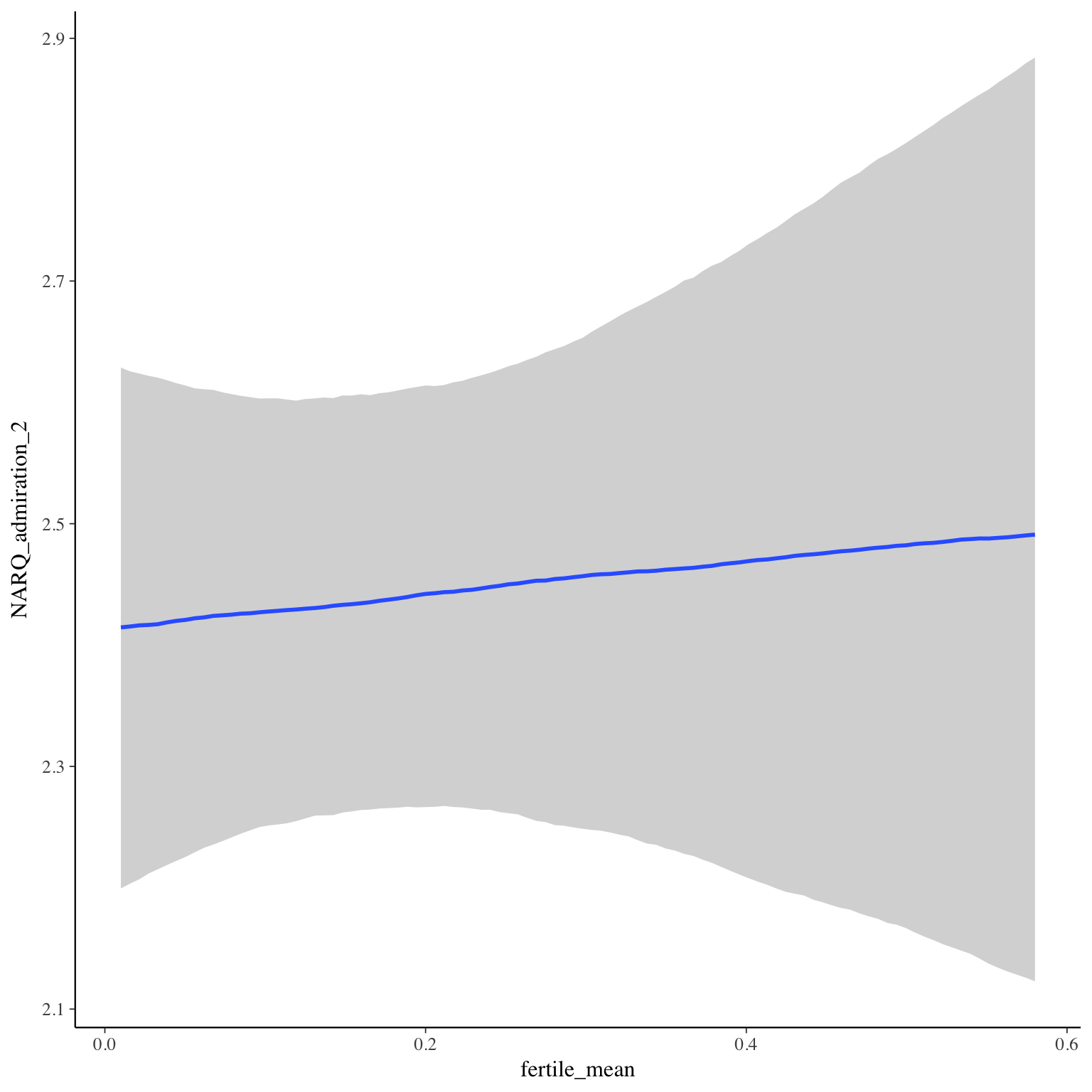
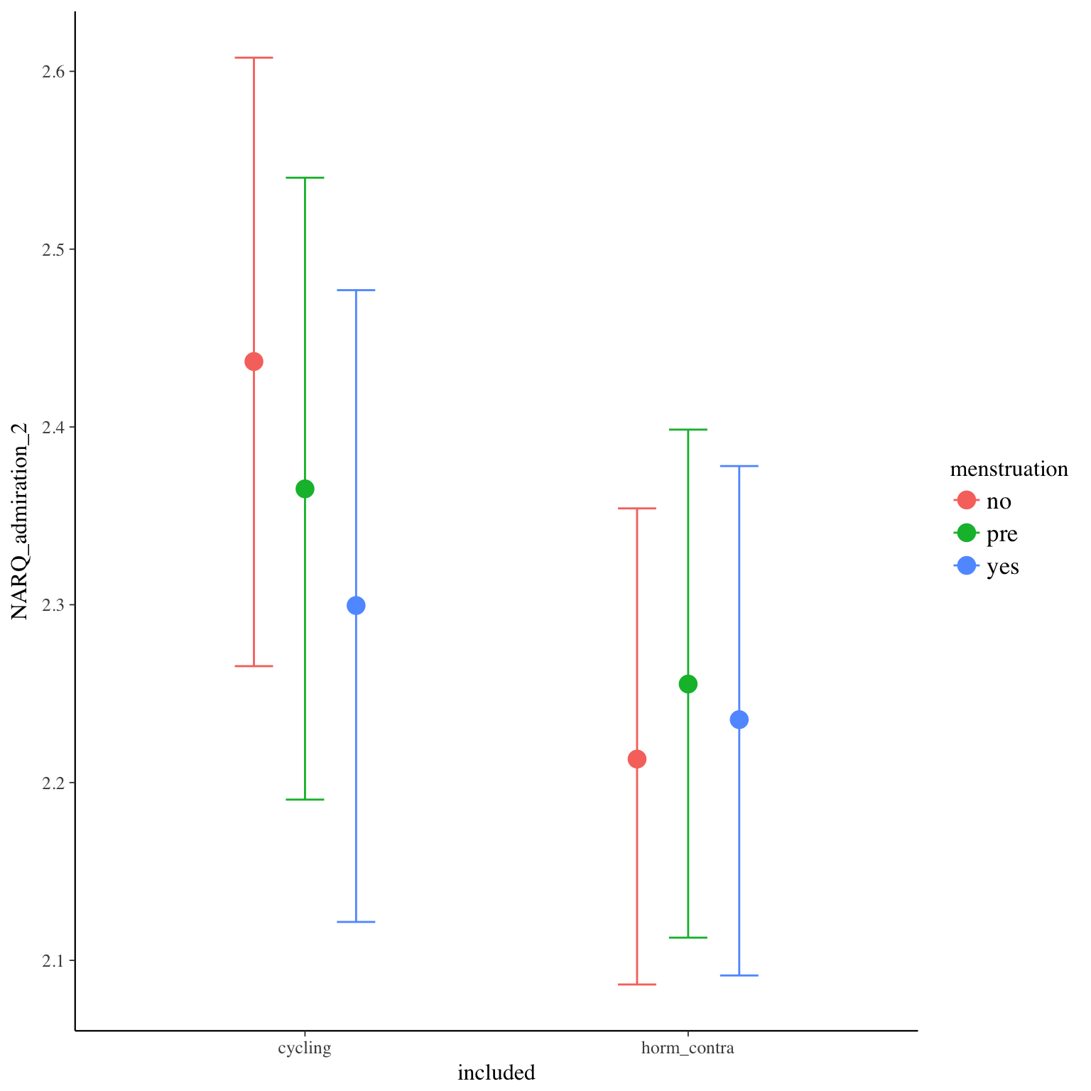
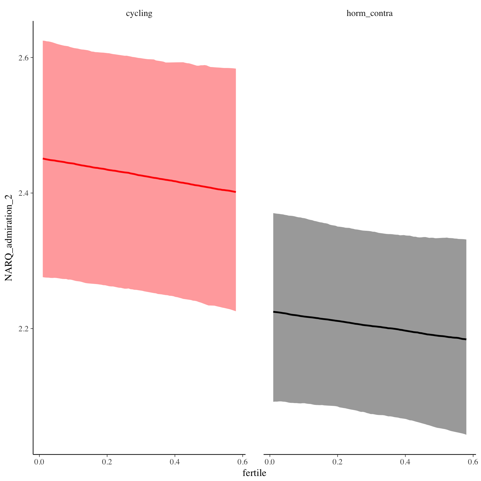
Diagnostics
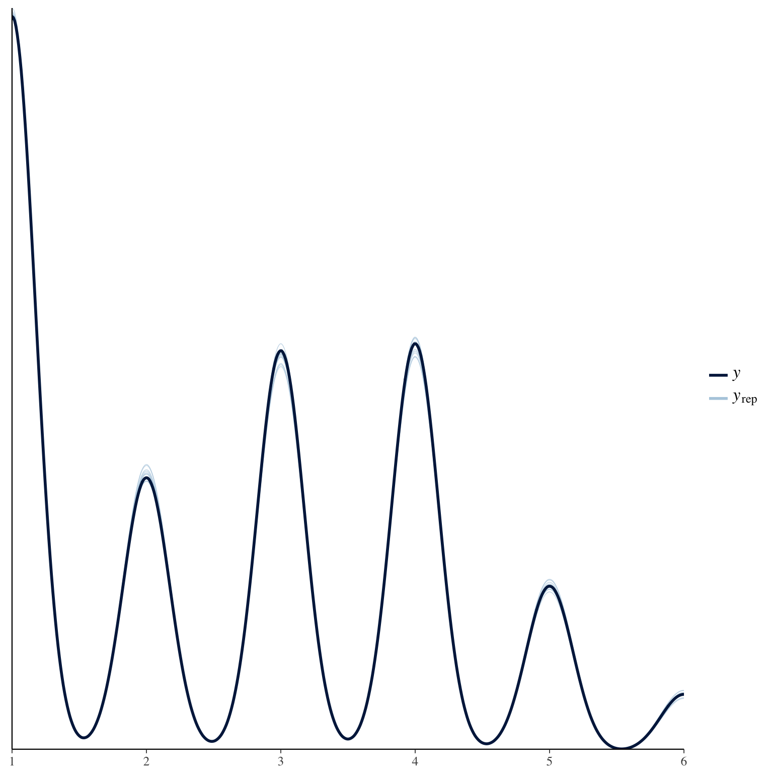
NARQ_admiration_3
Item text:
… habe ich es geschafft, mit meinen besonderen Beiträgen im Mittelpunkt zu stehen.
Item translation:
29. I managed to be the center of attention with my outstanding contributions
Choices:
| choice | value | frequency | percent |
|---|---|---|---|
| 1 | Stimme nicht zu | 11050 | 0.37 |
| 2 | Stimme überwiegend nicht zu | 3939 | 0.13 |
| 3 | Stimme eher nicht zu | 5601 | 0.19 |
| 4 | Stimme eher zu | 5852 | 0.2 |
| 5 | Stimme überwiegend zu | 2510 | 0.08 |
| 6 | Stimme voll zu | 925 | 0.03 |
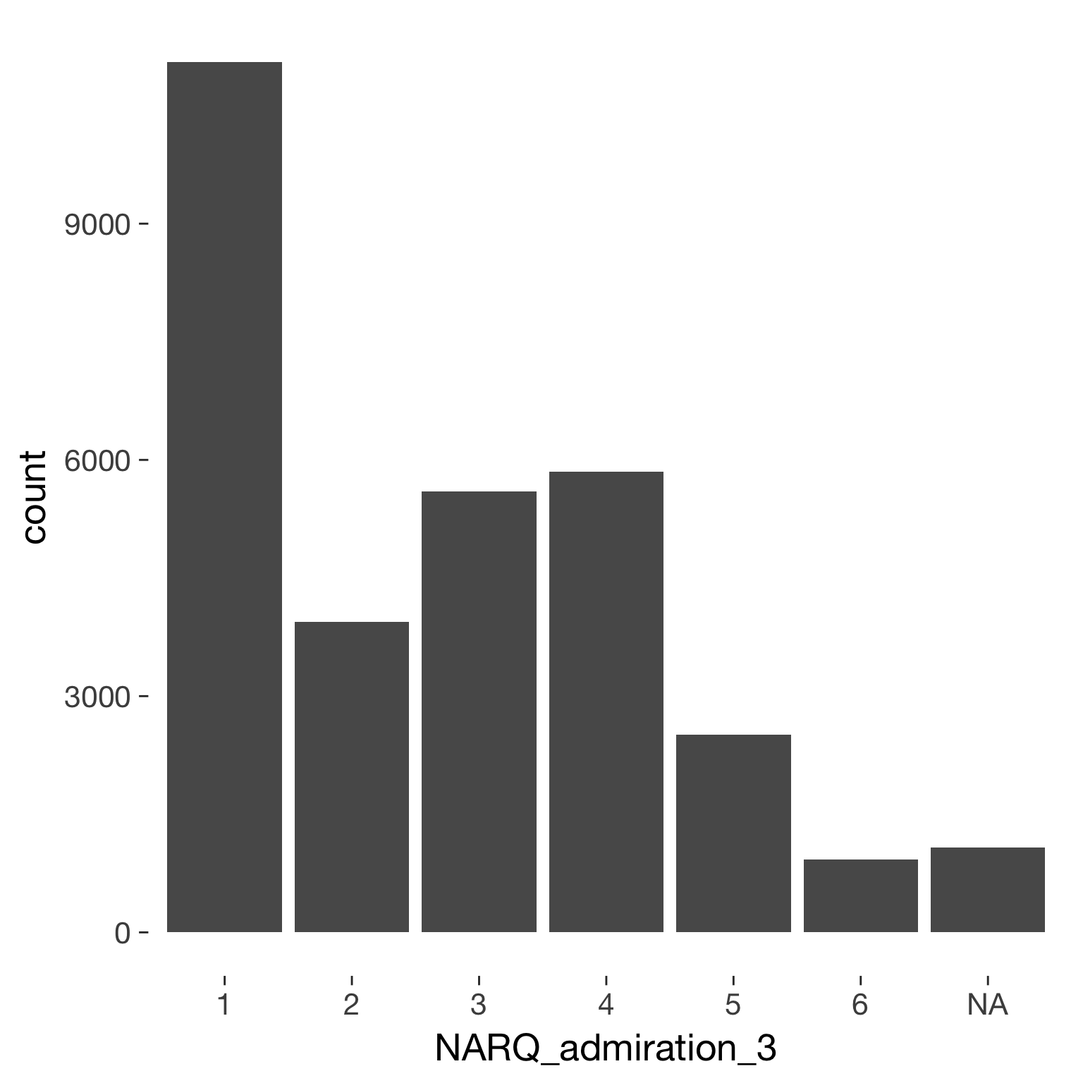
Model
Model summary
 Family: cumulative(logit)
Formula: NARQ_admiration_3 ~ included * (menstruation + fertile) + fertile_mean + (1 + fertile + menstruation | person)
         disc = 1
   Data: diary (Number of observations: 26546)
Samples: 4 chains, each with iter = 2000; warmup = 1000; thin = 1;
         total post-warmup samples = 4000
    ICs: LOO = 64972.74; WAIC = Not computed

Group-Level Effects:
~person (Number of levels: 1043)
                                     Estimate Est.Error l-95% CI u-95% CI Eff.Sample Rhat
sd(Intercept)                            2.32      0.07     2.19     2.46        532 1.00
sd(fertile)                              1.47      0.13     1.21     1.73        575 1.00
sd(menstruationpre)                      0.55      0.08     0.37     0.70        379 1.00
sd(menstruationyes)                      0.72      0.07     0.59     0.85        564 1.00
cor(Intercept,fertile)                  -0.17      0.08    -0.33    -0.01       2093 1.00
cor(Intercept,menstruationpre)          -0.28      0.10    -0.47    -0.09       1991 1.00
cor(fertile,menstruationpre)             0.22      0.15    -0.11     0.48        332 1.00
cor(Intercept,menstruationyes)          -0.25      0.08    -0.40    -0.09       1857 1.00
cor(fertile,menstruationyes)             0.33      0.11     0.10     0.54        312 1.01
cor(menstruationpre,menstruationyes)     0.69      0.11     0.46     0.88        143 1.02

Population-Level Effects:
                                    Estimate Est.Error l-95% CI u-95% CI Eff.Sample Rhat
Intercept[1]                           -0.87      0.17    -1.19    -0.54        316 1.01
Intercept[2]                            0.19      0.17    -0.13     0.52        317 1.01
Intercept[3]                            1.54      0.17     1.22     1.87        316 1.01
Intercept[4]                            3.35      0.17     3.03     3.68        316 1.01
Intercept[5]                            5.08      0.17     4.75     5.42        332 1.01
includedhorm_contra                    -0.21      0.15    -0.51     0.09        232 1.01
menstruationpre                        -0.07      0.07    -0.21     0.06       1780 1.00
menstruationyes                        -0.16      0.07    -0.31    -0.03       1460 1.00
fertile                                 0.02      0.15    -0.28     0.32       1919 1.00
fertile_mean                            0.26      0.67    -1.03     1.69        613 1.00
includedhorm_contra:menstruationpre     0.03      0.09    -0.14     0.21       1982 1.00
includedhorm_contra:menstruationyes     0.14      0.09    -0.04     0.31       1755 1.00
includedhorm_contra:fertile            -0.09      0.18    -0.45     0.28       1971 1.00

Samples were drawn using sampling(NUTS). For each parameter, Eff.Sample
is a crude measure of effective sample size, and Rhat is the potential
scale reduction factor on split chains (at convergence, Rhat = 1).
Coefficient plot
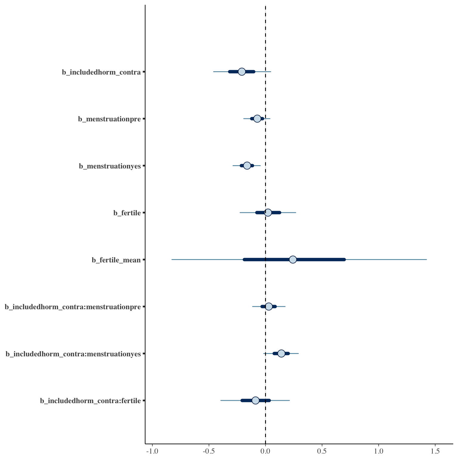
Marginal effect plots


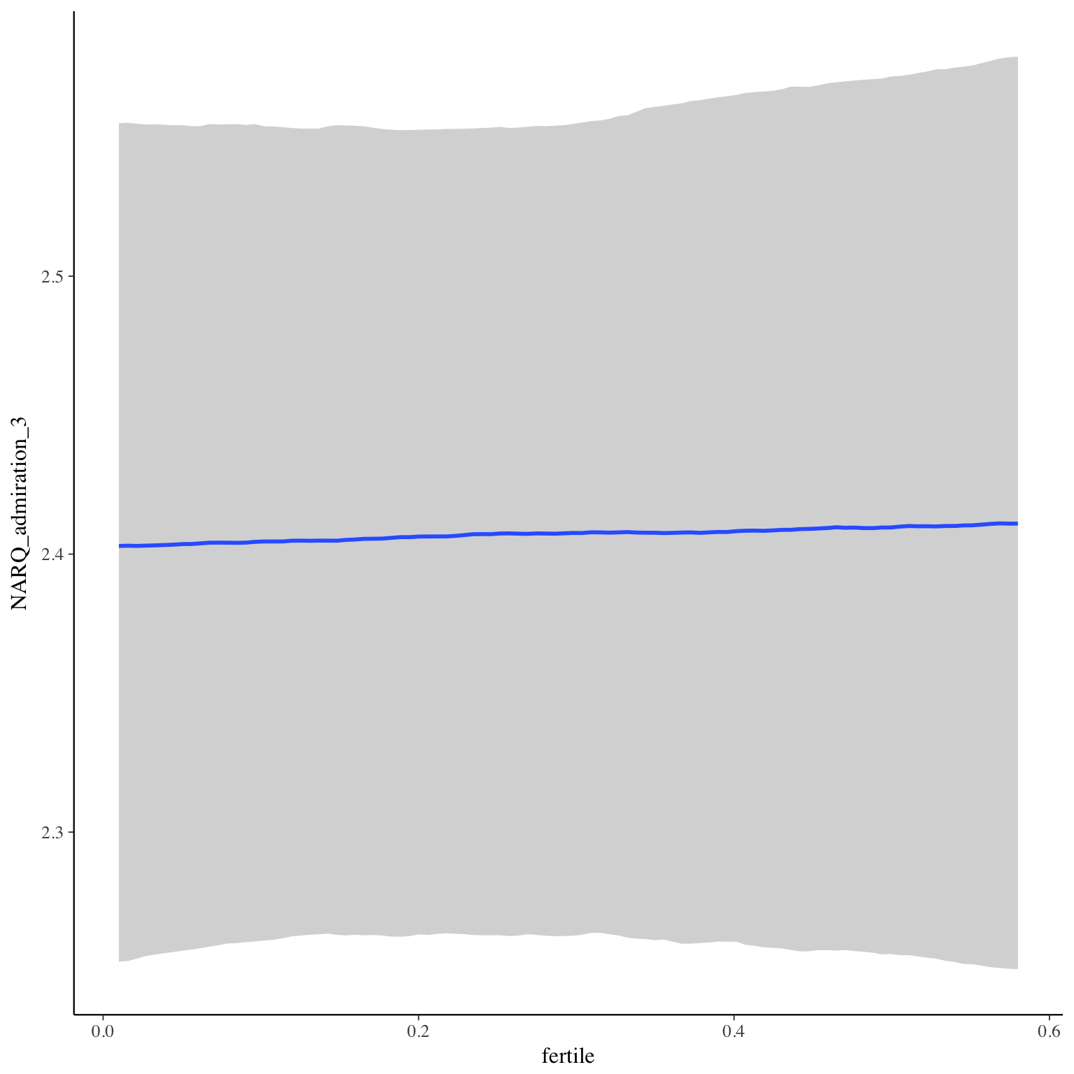
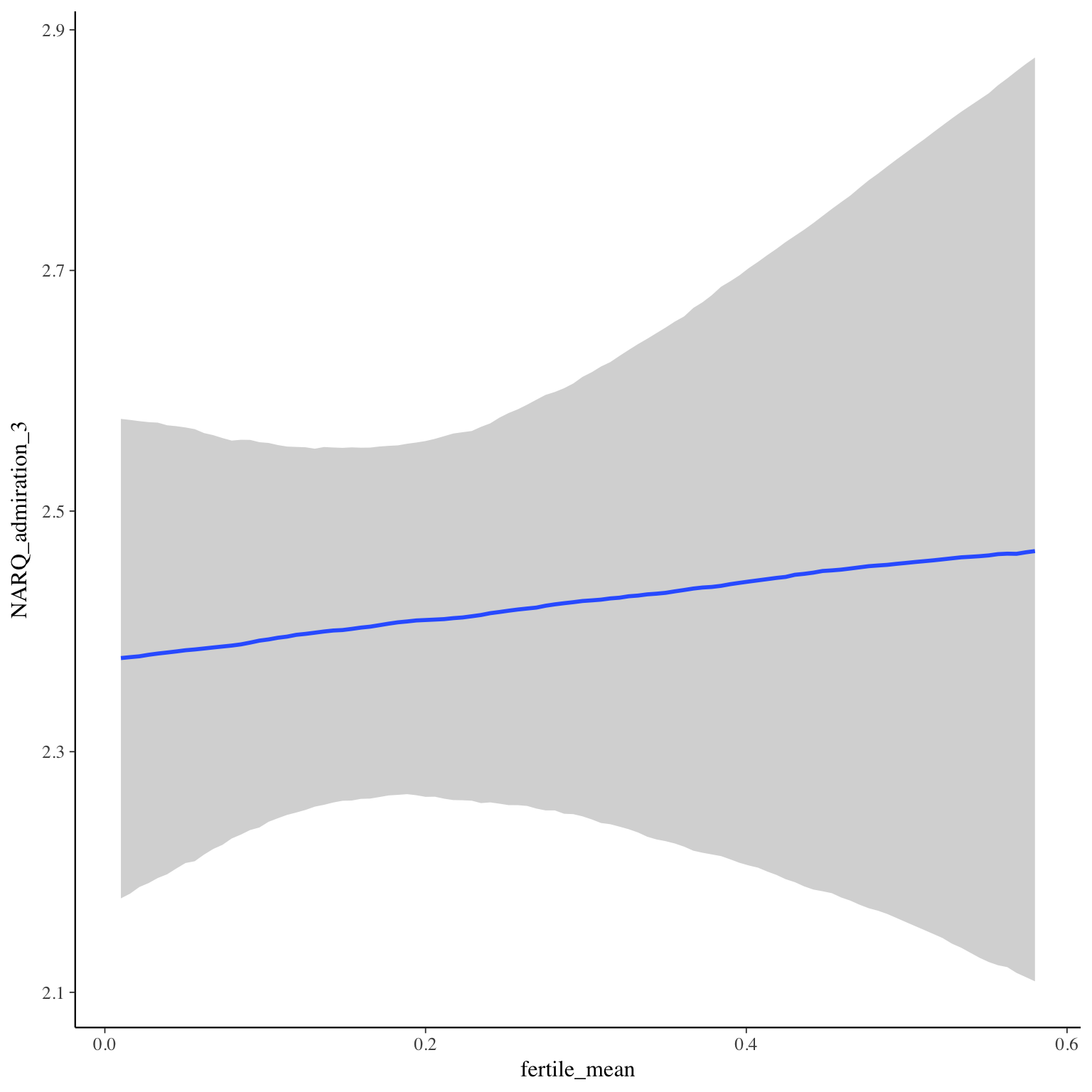
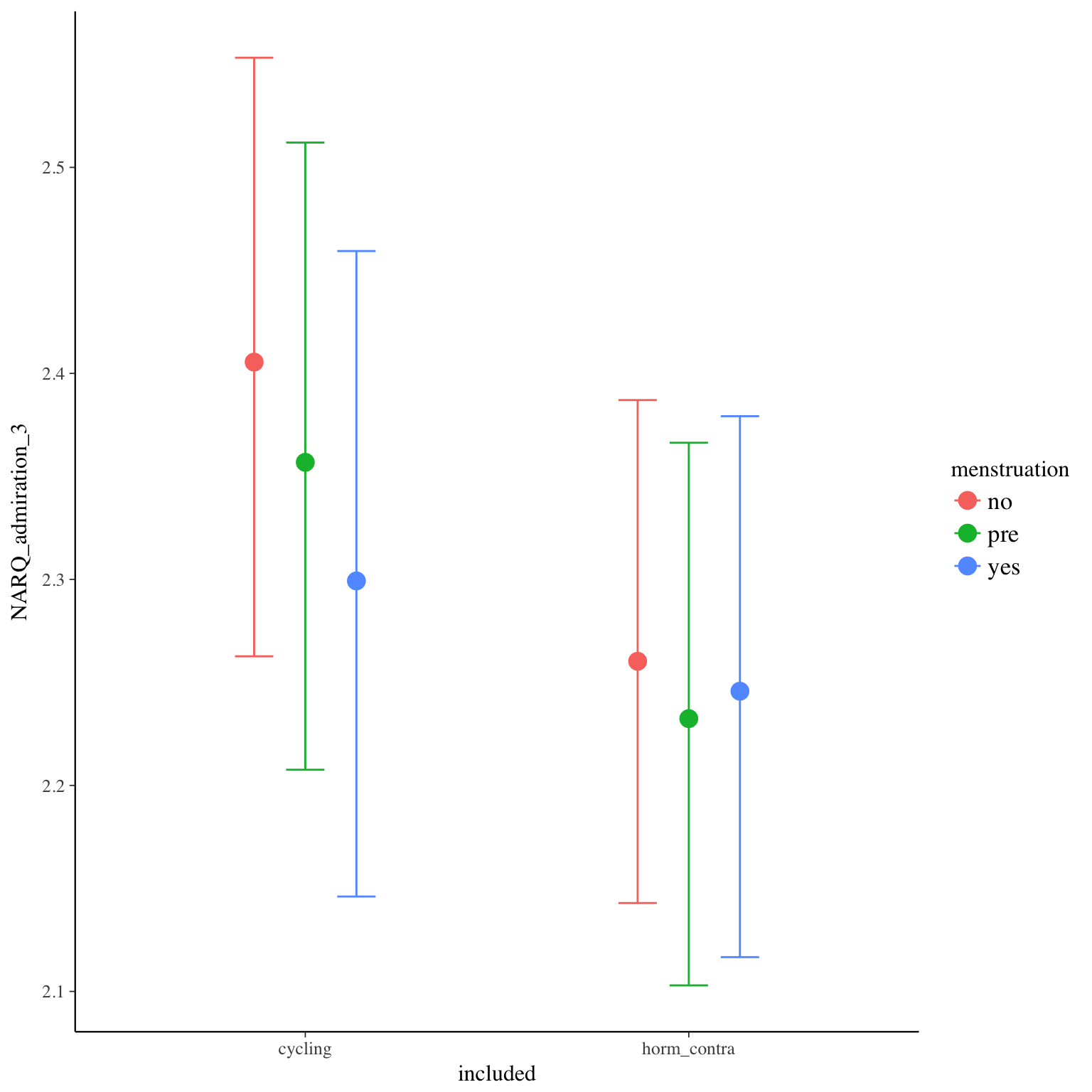
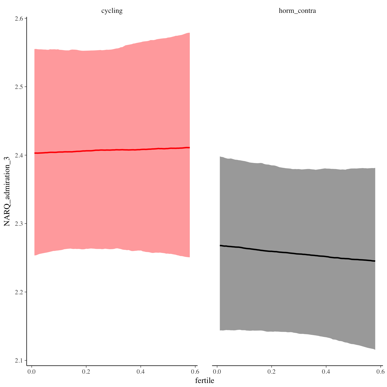
Diagnostics
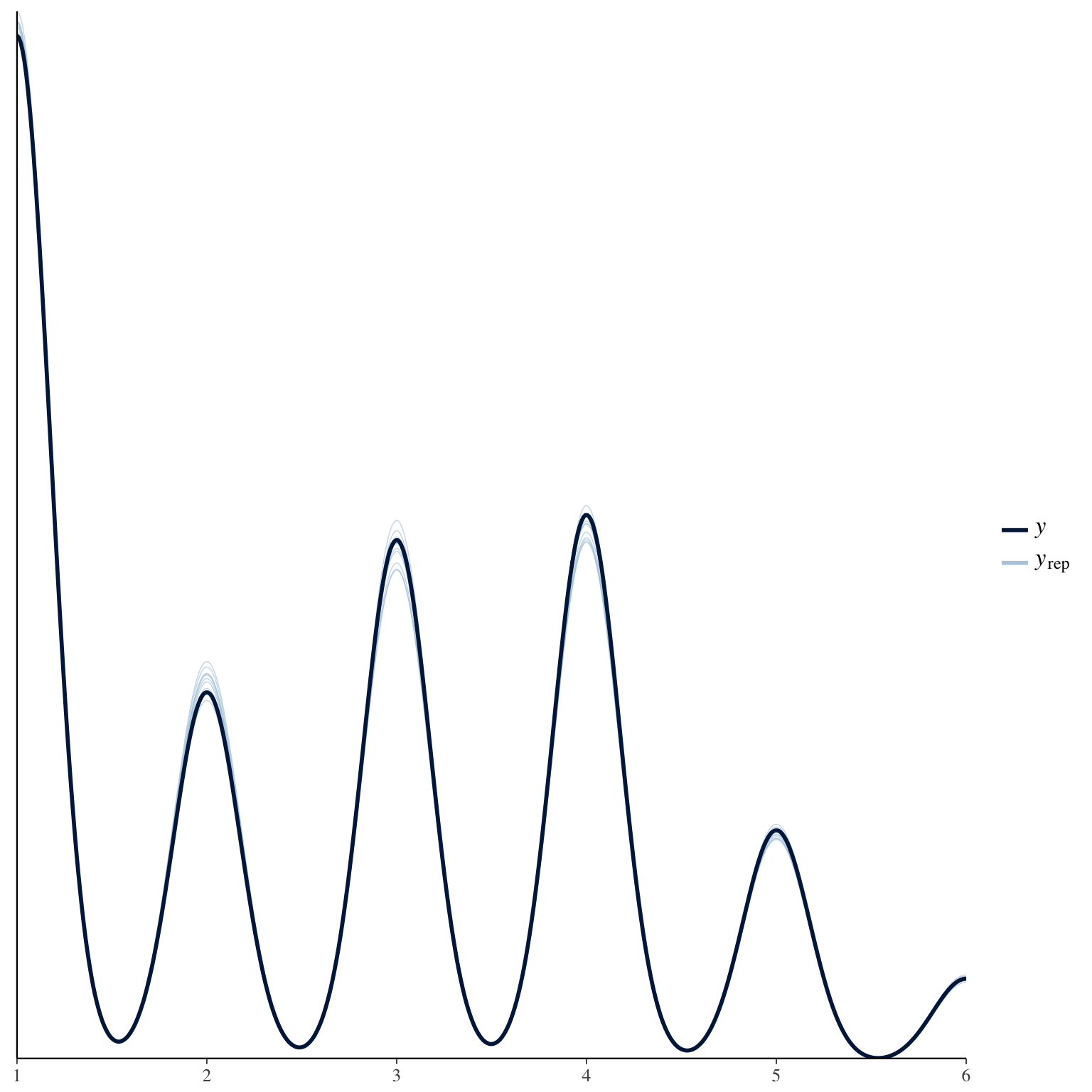
NARQ_rivalry_1
Item text:
… habe ich genervt reagiert, wenn eine andere Frau mir die Schau gestohlen hat.
Item translation:
30. I reacted annoyed when another woman stole the show from me.
Choices:
| choice | value | frequency | percent |
|---|---|---|---|
| 1 | Stimme nicht zu | 24605 | 0.82 |
| 2 | Stimme überwiegend nicht zu | 2457 | 0.08 |
| 3 | Stimme eher nicht zu | 1357 | 0.05 |
| 4 | Stimme eher zu | 960 | 0.03 |
| 5 | Stimme überwiegend zu | 276 | 0.01 |
| 6 | Stimme voll zu | 221 | 0.01 |

Model
Model summary
 Family: cumulative(logit)
Formula: NARQ_rivalry_1 ~ included * (menstruation + fertile) + fertile_mean + (1 + fertile + menstruation | person)
         disc = 1
   Data: diary (Number of observations: 26545)
Samples: 4 chains, each with iter = 2000; warmup = 1000; thin = 1;
         total post-warmup samples = 4000
    ICs: LOO = 29128.25; WAIC = Not computed

Group-Level Effects:
~person (Number of levels: 1043)
                                     Estimate Est.Error l-95% CI u-95% CI Eff.Sample Rhat
sd(Intercept)                            2.07      0.08     1.92     2.22        730 1.01
sd(fertile)                              1.15      0.22     0.72     1.58        520 1.01
sd(menstruationpre)                      0.26      0.14     0.01     0.52        337 1.01
sd(menstruationyes)                      0.28      0.14     0.02     0.55        523 1.01
cor(Intercept,fertile)                  -0.32      0.13    -0.57    -0.06       4000 1.00
cor(Intercept,menstruationpre)          -0.02      0.30    -0.62     0.58       4000 1.00
cor(fertile,menstruationpre)            -0.29      0.36    -0.87     0.51       1061 1.01
cor(Intercept,menstruationyes)           0.04      0.28    -0.57     0.62       4000 1.00
cor(fertile,menstruationyes)             0.38      0.33    -0.38     0.88        873 1.00
cor(menstruationpre,menstruationyes)    -0.29      0.40    -0.90     0.60        960 1.00

Population-Level Effects:
                                    Estimate Est.Error l-95% CI u-95% CI Eff.Sample Rhat
Intercept[1]                            2.40      0.17     2.06     2.75       1413    1
Intercept[2]                            3.49      0.18     3.15     3.84       1421    1
Intercept[3]                            4.42      0.18     4.08     4.78       1445    1
Intercept[4]                            5.75      0.18     5.40     6.12       1527    1
Intercept[5]                            6.70      0.19     6.32     7.08       1631    1
includedhorm_contra                     0.10      0.16    -0.21     0.41       1099    1
menstruationpre                        -0.18      0.11    -0.40     0.04       4000    1
menstruationyes                        -0.08      0.11    -0.29     0.12       4000    1
fertile                                 0.09      0.23    -0.36     0.53       4000    1
fertile_mean                           -0.20      0.69    -1.59     1.15       2406    1
includedhorm_contra:menstruationpre     0.19      0.12    -0.05     0.42       4000    1
includedhorm_contra:menstruationyes    -0.01      0.12    -0.23     0.21       4000    1
includedhorm_contra:fertile             0.00      0.25    -0.49     0.49       4000    1

Samples were drawn using sampling(NUTS). For each parameter, Eff.Sample
is a crude measure of effective sample size, and Rhat is the potential
scale reduction factor on split chains (at convergence, Rhat = 1).
Coefficient plot
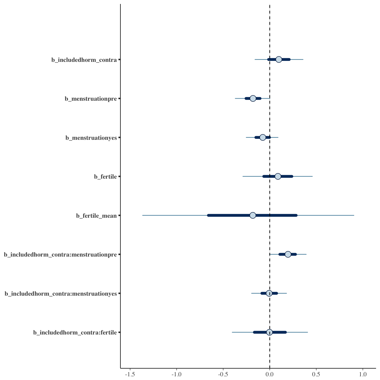
Marginal effect plots
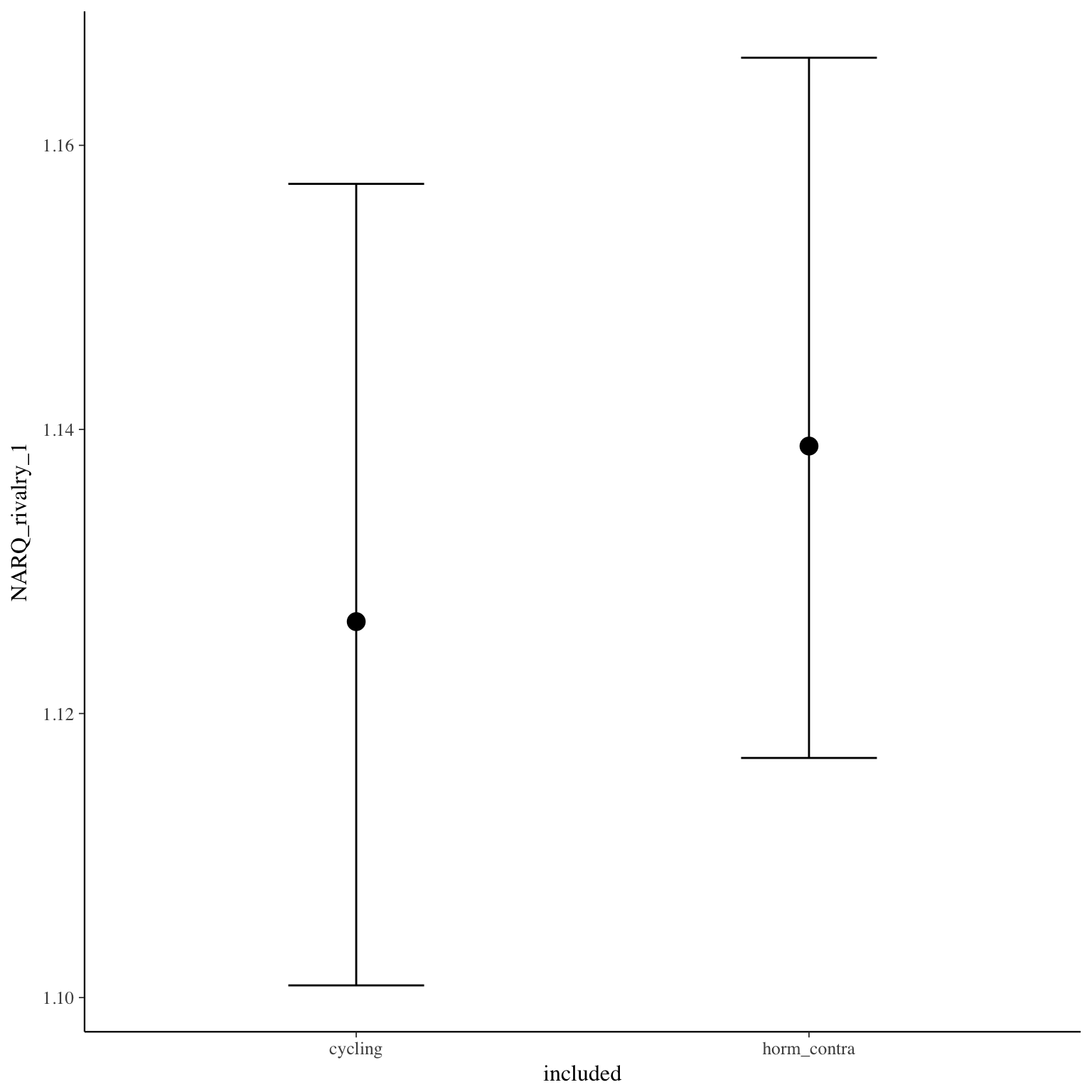
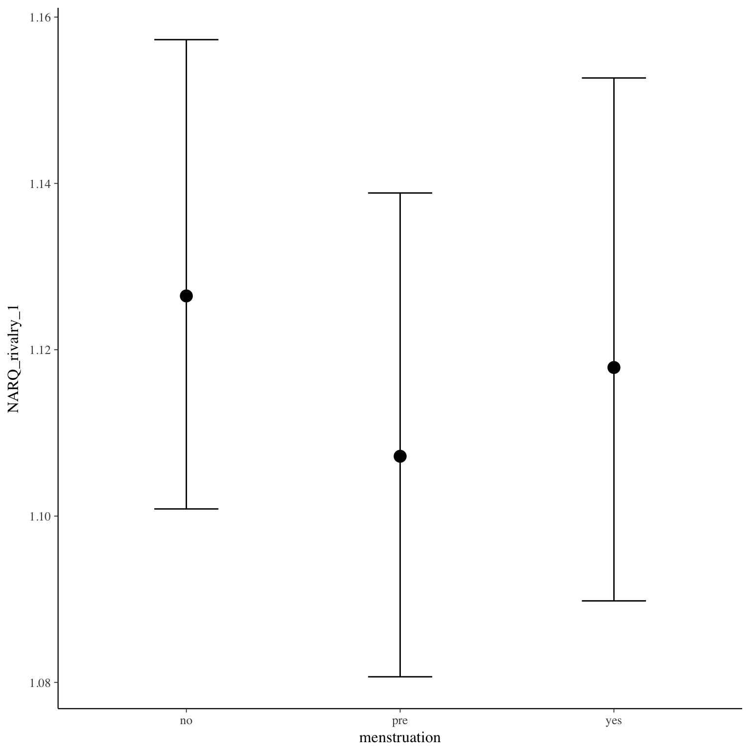
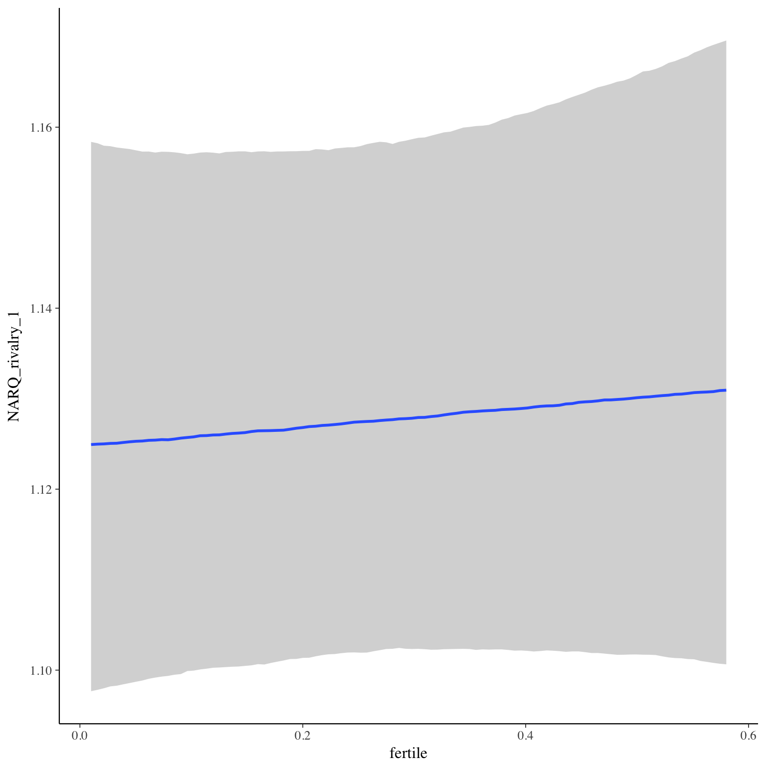
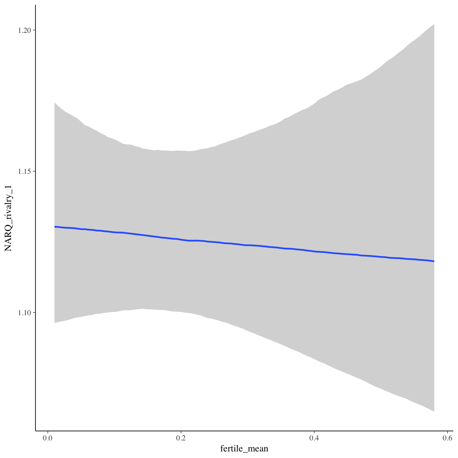
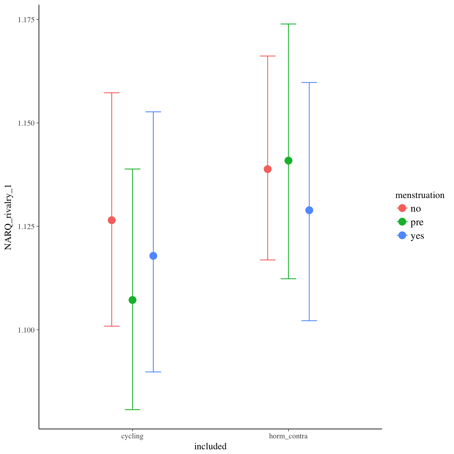
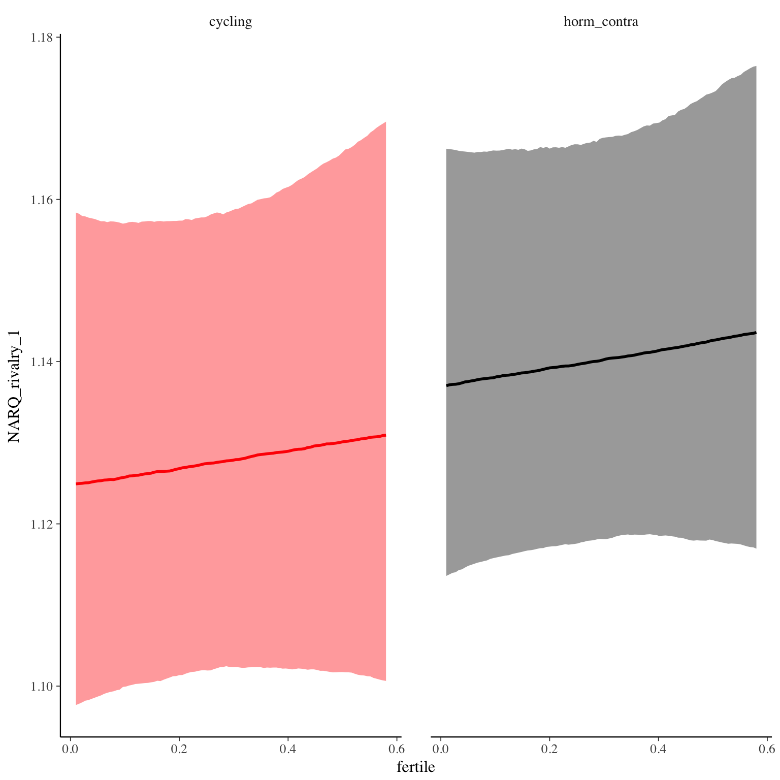
Diagnostics
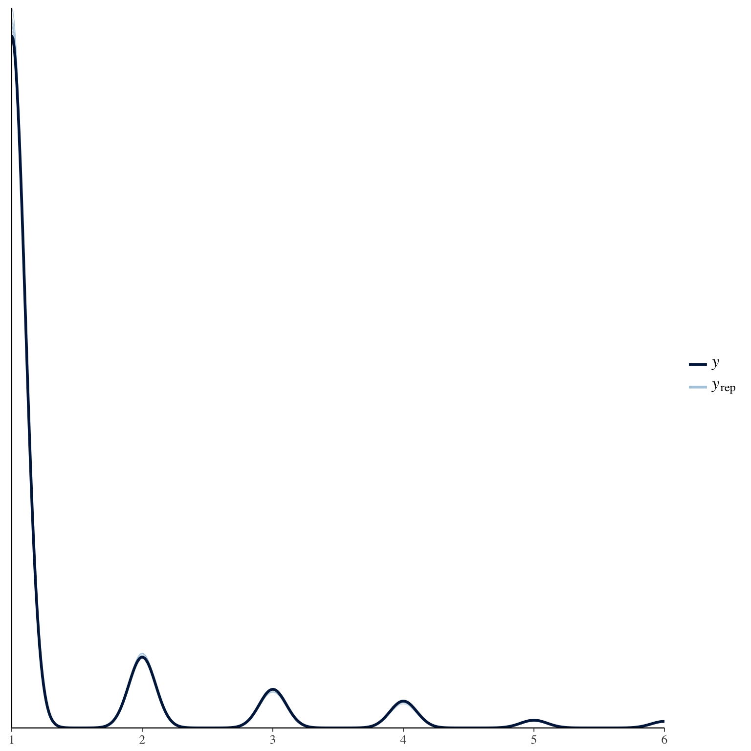
NARQ_rivalry_2
Item text:
… wollte ich, dass meine Konkurrentinnen sich blamieren oder ignoriert werden.
Item translation:
31. I wanted my female rivals to fail.
Choices:
| choice | value | frequency | percent |
|---|---|---|---|
| 1 | Stimme nicht zu | 25617 | 0.86 |
| 2 | Stimme überwiegend nicht zu | 1753 | 0.06 |
| 3 | Stimme eher nicht zu | 960 | 0.03 |
| 4 | Stimme eher zu | 894 | 0.03 |
| 5 | Stimme überwiegend zu | 321 | 0.01 |
| 6 | Stimme voll zu | 332 | 0.01 |
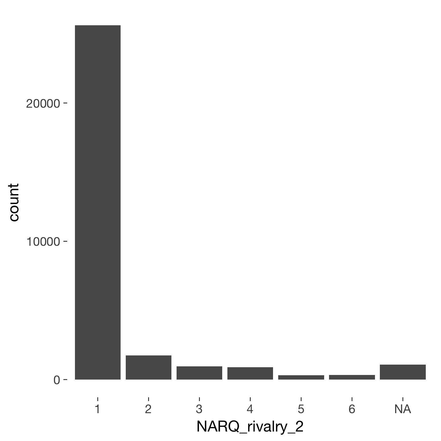
Model
Model summary
 Family: cumulative(logit)
Formula: NARQ_rivalry_2 ~ included * (menstruation + fertile) + fertile_mean + (1 + fertile + menstruation | person)
         disc = 1
   Data: diary (Number of observations: 26546)
Samples: 4 chains, each with iter = 2000; warmup = 1000; thin = 1;
         total post-warmup samples = 4000
    ICs: LOO = 24128.93; WAIC = Not computed

Group-Level Effects:
~person (Number of levels: 1043)
                                     Estimate Est.Error l-95% CI u-95% CI Eff.Sample Rhat
sd(Intercept)                            2.39      0.10     2.20     2.58        664 1.01
sd(fertile)                              1.77      0.22     1.33     2.21        518 1.00
sd(menstruationpre)                      0.28      0.17     0.02     0.62        272 1.01
sd(menstruationyes)                      0.63      0.16     0.24     0.92        295 1.01
cor(Intercept,fertile)                  -0.17      0.12    -0.39     0.07       2604 1.00
cor(Intercept,menstruationpre)           0.04      0.33    -0.64     0.66       2725 1.00
cor(fertile,menstruationpre)            -0.23      0.36    -0.86     0.51        561 1.00
cor(Intercept,menstruationyes)          -0.09      0.18    -0.43     0.26       1327 1.00
cor(fertile,menstruationyes)             0.01      0.22    -0.47     0.39        395 1.00
cor(menstruationpre,menstruationyes)     0.27      0.40    -0.65     0.86        100 1.04

Population-Level Effects:
                                    Estimate Est.Error l-95% CI u-95% CI Eff.Sample Rhat
Intercept[1]                            3.21      0.21     2.82     3.63        832 1.00
Intercept[2]                            4.13      0.21     3.75     4.55        845 1.00
Intercept[3]                            4.88      0.21     4.48     5.29        862 1.00
Intercept[4]                            6.10      0.21     5.69     6.52        876 1.00
Intercept[5]                            7.03      0.22     6.62     7.46        938 1.00
includedhorm_contra                     0.27      0.19    -0.10     0.65        576 1.01
menstruationpre                        -0.24      0.14    -0.52     0.02       2313 1.00
menstruationyes                        -0.14      0.15    -0.44     0.15       1352 1.00
fertile                                -0.27      0.30    -0.87     0.32       2067 1.00
fertile_mean                            0.43      0.78    -1.05     2.06       1430 1.00
includedhorm_contra:menstruationpre     0.11      0.14    -0.16     0.39       2686 1.00
includedhorm_contra:menstruationyes     0.04      0.15    -0.24     0.33       2575 1.00
includedhorm_contra:fertile            -0.03      0.30    -0.61     0.55       2479 1.00

Samples were drawn using sampling(NUTS). For each parameter, Eff.Sample
is a crude measure of effective sample size, and Rhat is the potential
scale reduction factor on split chains (at convergence, Rhat = 1).
Coefficient plot
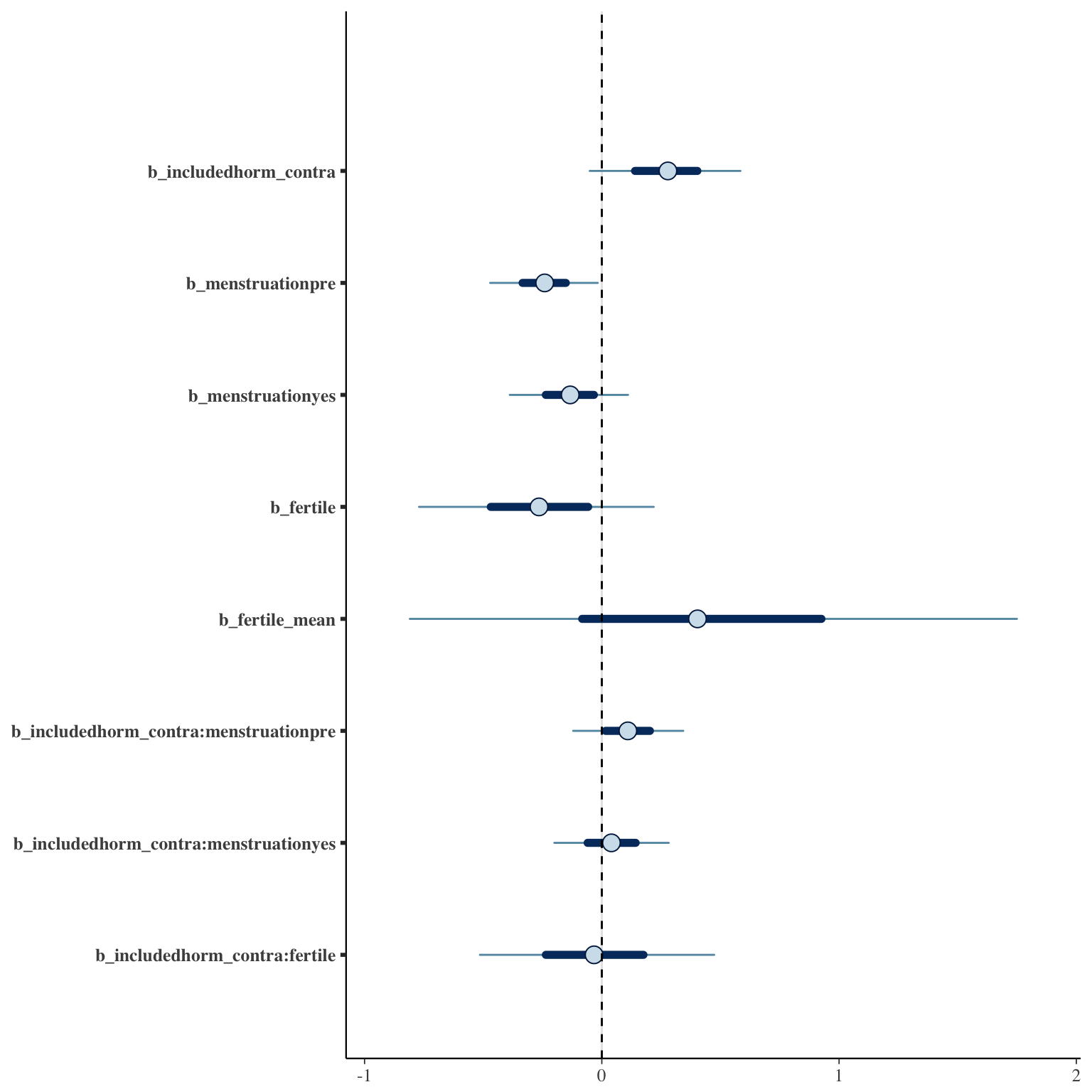
Marginal effect plots
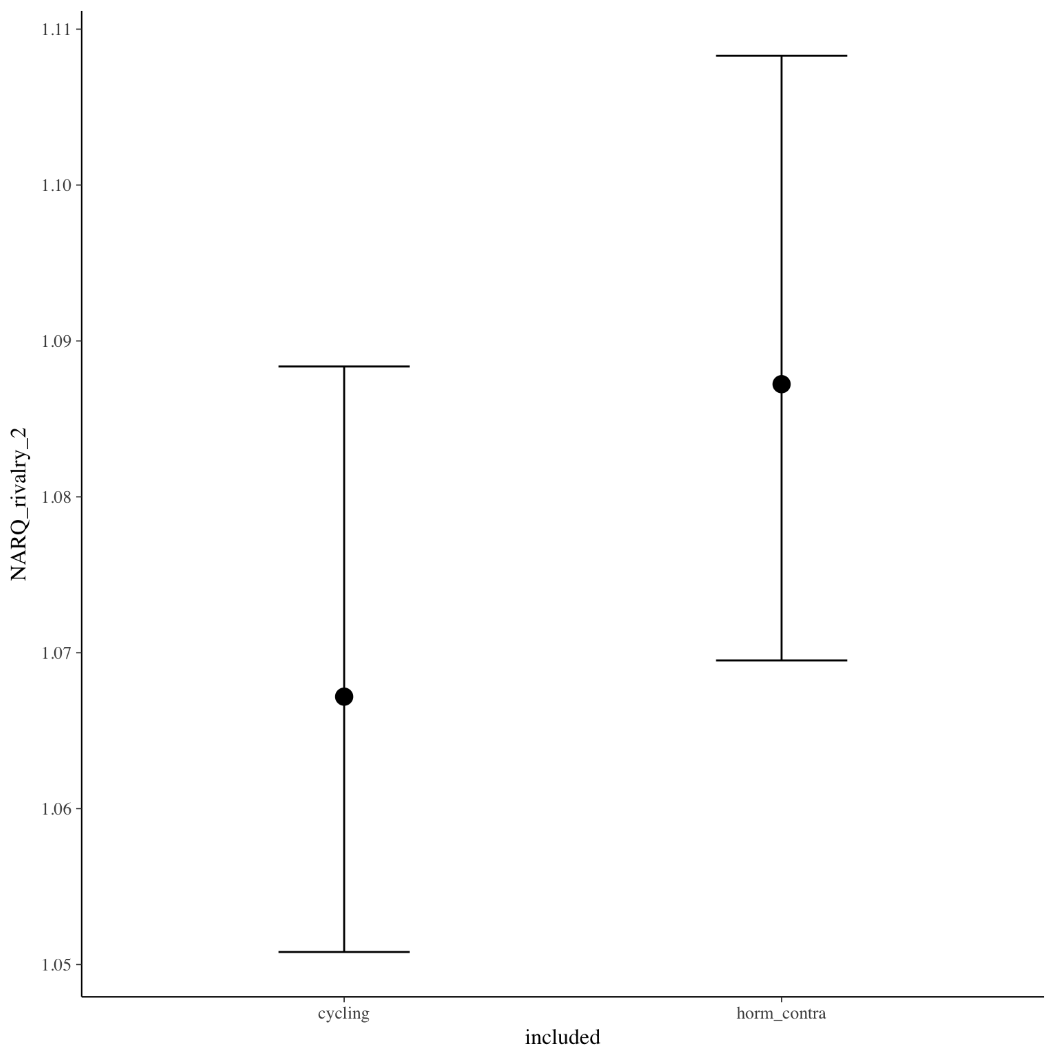
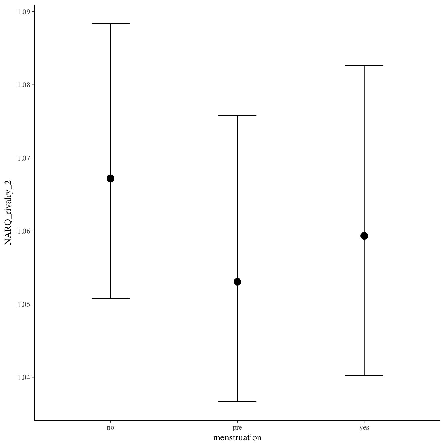
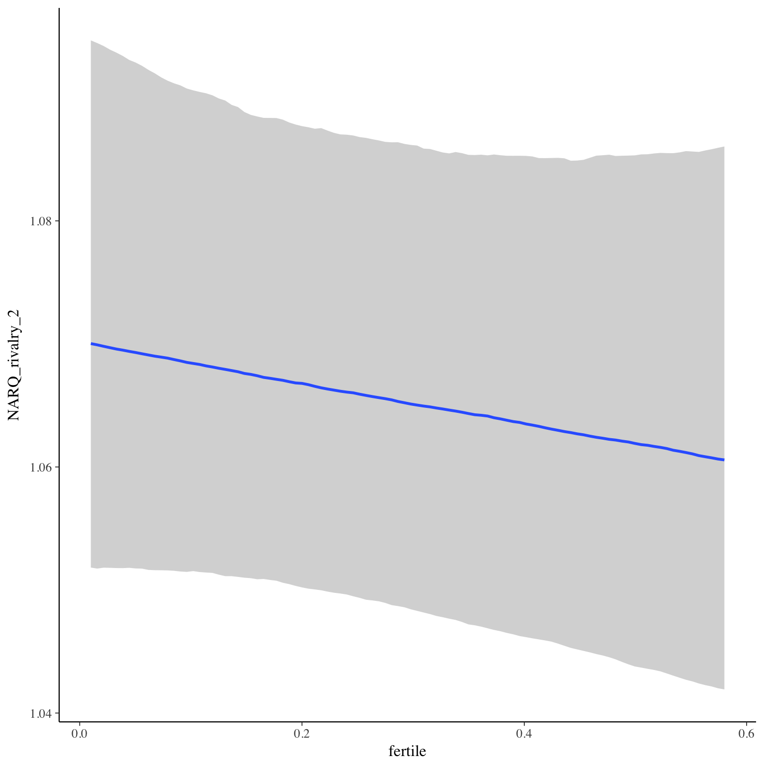
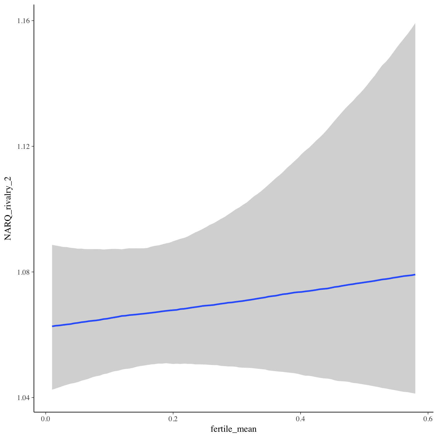
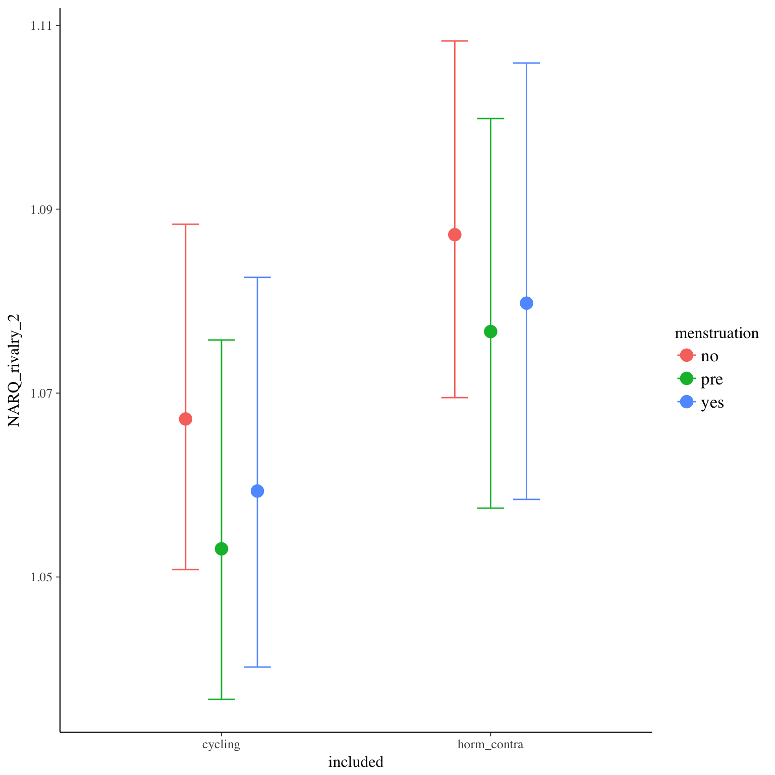
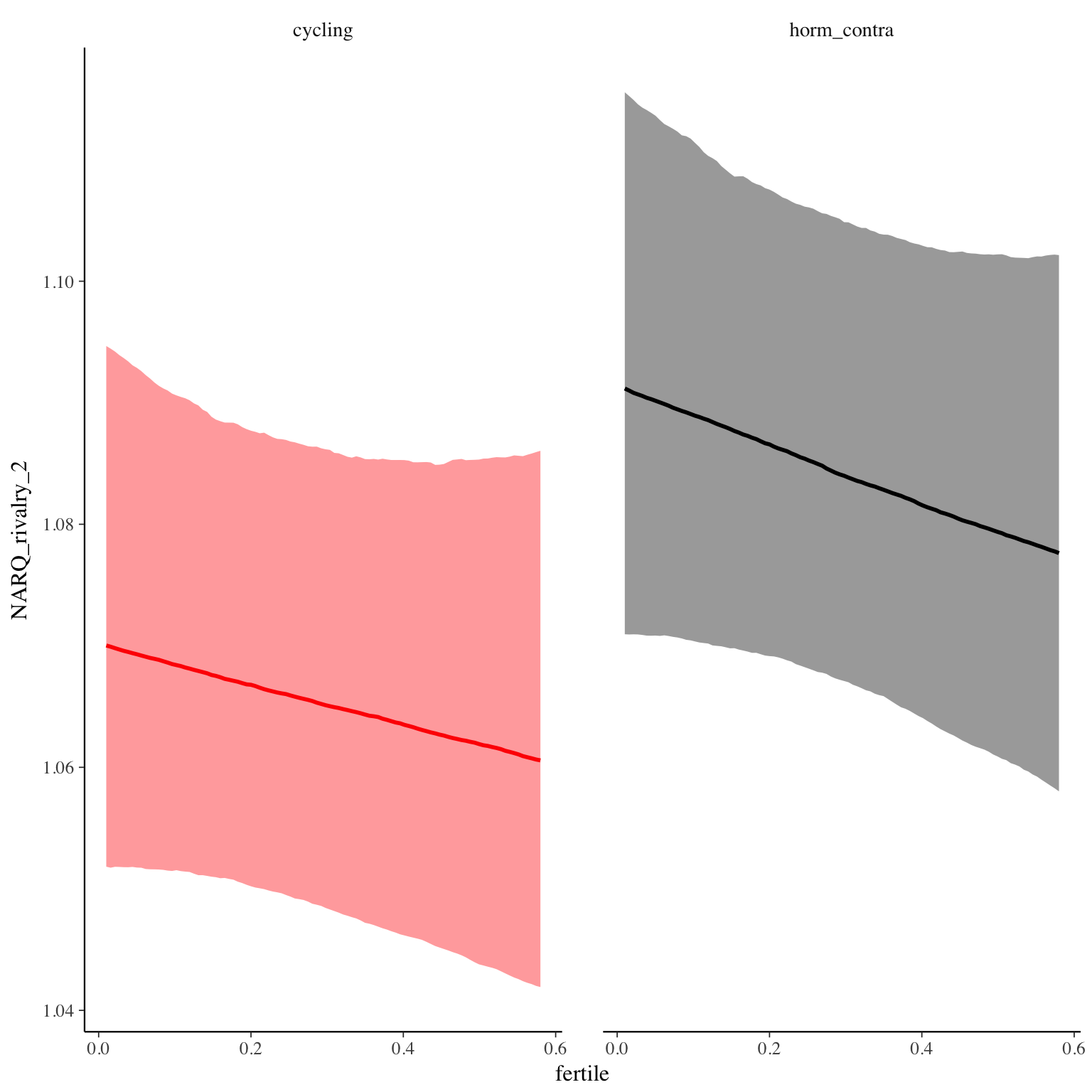
Diagnostics
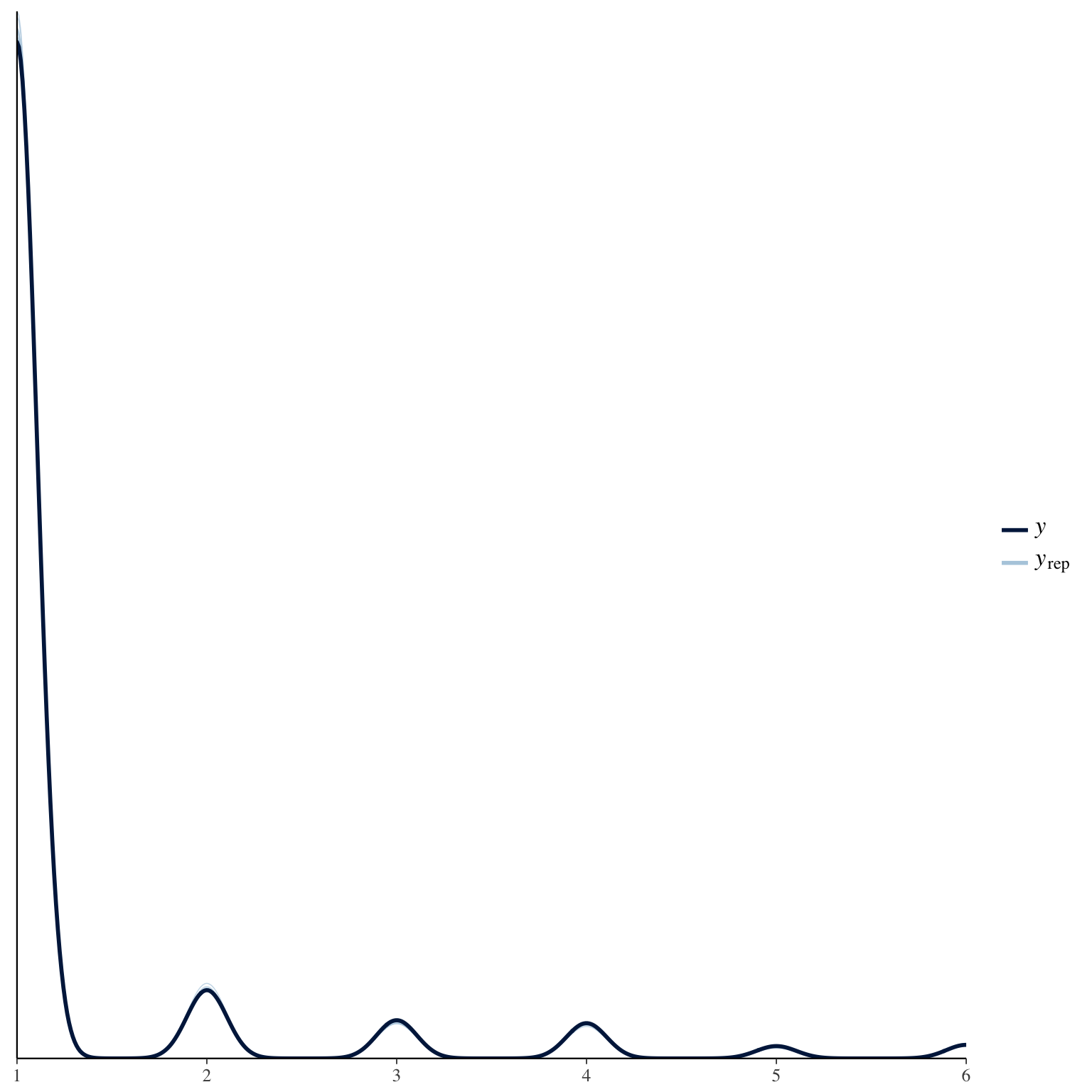
NARQ_rivalry_3
Item text:
… hatte ich das Gefühl, dass die meisten Frauen ziemliche Versagerinnen sind.
Item translation:
32. I had the feeling that most women are somehow losers.
Choices:
| choice | value | frequency | percent |
|---|---|---|---|
| 1 | Stimme nicht zu | 26119 | 0.87 |
| 2 | Stimme überwiegend nicht zu | 1829 | 0.06 |
| 3 | Stimme eher nicht zu | 1012 | 0.03 |
| 4 | Stimme eher zu | 611 | 0.02 |
| 5 | Stimme überwiegend zu | 202 | 0.01 |
| 6 | Stimme voll zu | 103 | 0 |
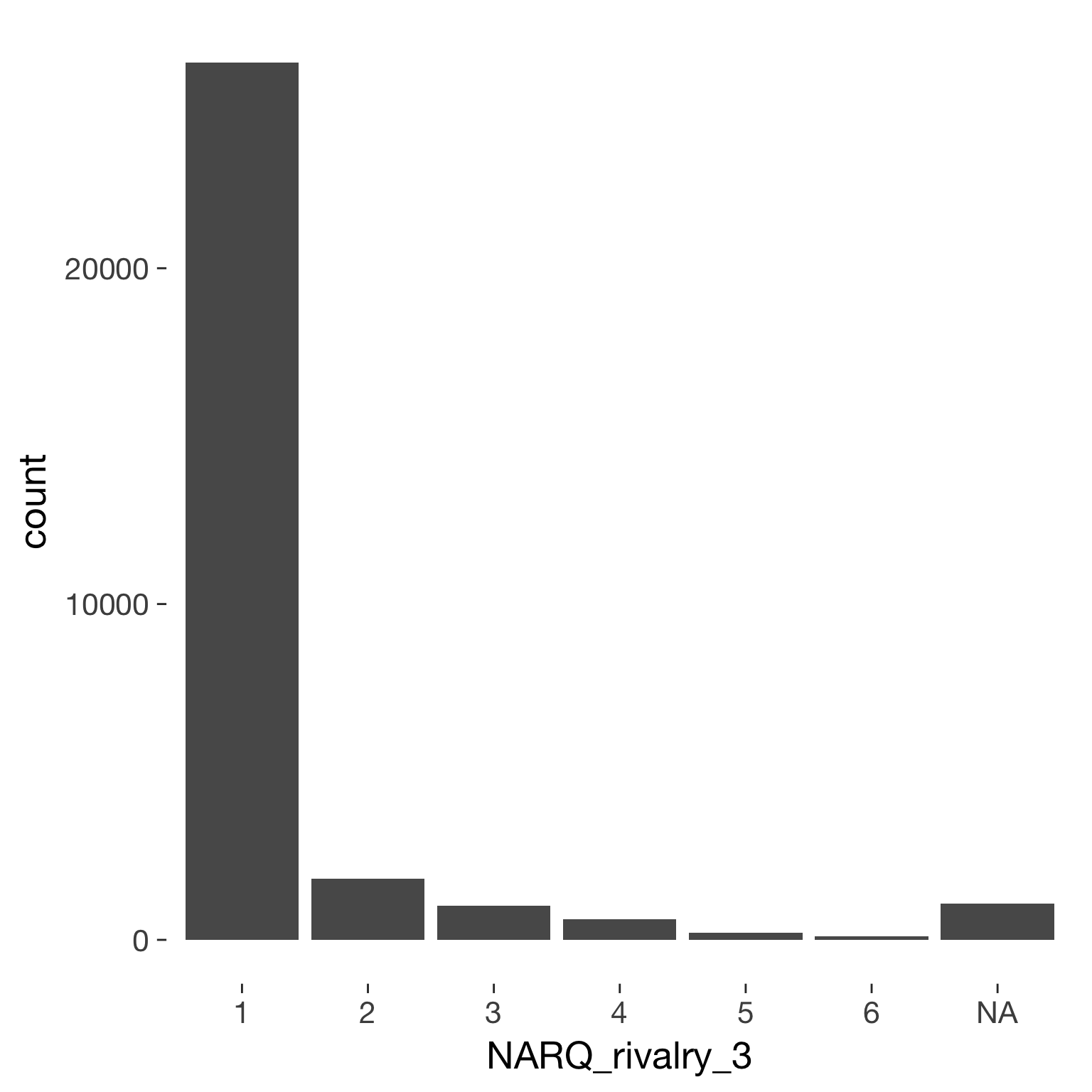
Model
Model summary
 Family: cumulative(logit)
Formula: NARQ_rivalry_3 ~ included * (menstruation + fertile) + fertile_mean + (1 + fertile + menstruation | person)
         disc = 1
   Data: diary (Number of observations: 26545)
Samples: 4 chains, each with iter = 2000; warmup = 1000; thin = 1;
         total post-warmup samples = 4000
    ICs: LOO = 19471.11; WAIC = Not computed

Group-Level Effects:
~person (Number of levels: 1043)
                                     Estimate Est.Error l-95% CI u-95% CI Eff.Sample Rhat
sd(Intercept)                            2.76      0.12     2.54     3.00        854 1.00
sd(fertile)                              1.39      0.24     0.91     1.87        790 1.01
sd(menstruationpre)                      0.48      0.14     0.19     0.75        529 1.00
sd(menstruationyes)                      0.38      0.21     0.02     0.76        268 1.01
cor(Intercept,fertile)                  -0.07      0.16    -0.39     0.25       4000 1.00
cor(Intercept,menstruationpre)           0.00      0.23    -0.48     0.46       2556 1.00
cor(fertile,menstruationpre)            -0.58      0.24    -0.94    -0.02        680 1.00
cor(Intercept,menstruationyes)          -0.08      0.29    -0.66     0.52       4000 1.00
cor(fertile,menstruationyes)             0.14      0.34    -0.60     0.73       1020 1.00
cor(menstruationpre,menstruationyes)     0.11      0.38    -0.69     0.75        711 1.00

Population-Level Effects:
                                    Estimate Est.Error l-95% CI u-95% CI Eff.Sample Rhat
Intercept[1]                            3.74      0.24     3.26     4.21        786    1
Intercept[2]                            4.96      0.24     4.49     5.44        800    1
Intercept[3]                            6.09      0.25     5.60     6.56        817    1
Intercept[4]                            7.60      0.25     7.10     8.10        850    1
Intercept[5]                            8.91      0.27     8.37     9.45        930    1
includedhorm_contra                     0.27      0.22    -0.16     0.70        698    1
menstruationpre                        -0.09      0.17    -0.42     0.23       3101    1
menstruationyes                         0.18      0.15    -0.13     0.47       2417    1
fertile                                -0.16      0.33    -0.81     0.48       2999    1
fertile_mean                           -0.20      0.86    -2.00     1.44       1895    1
includedhorm_contra:menstruationpre     0.09      0.16    -0.21     0.39       4000    1
includedhorm_contra:menstruationyes    -0.17      0.14    -0.45     0.11       4000    1
includedhorm_contra:fertile            -0.15      0.31    -0.76     0.47       4000    1

Samples were drawn using sampling(NUTS). For each parameter, Eff.Sample
is a crude measure of effective sample size, and Rhat is the potential
scale reduction factor on split chains (at convergence, Rhat = 1).
Coefficient plot
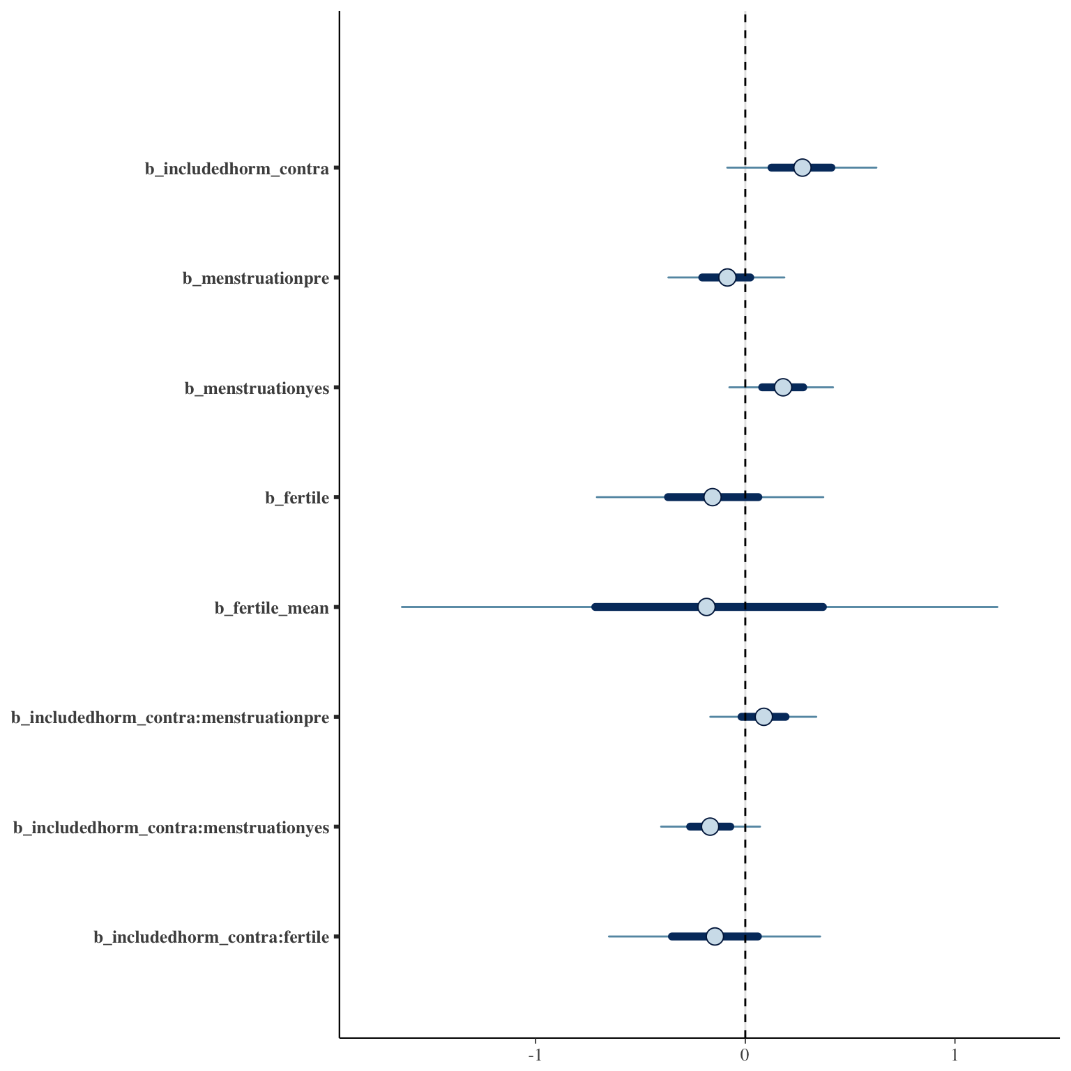
Marginal effect plots
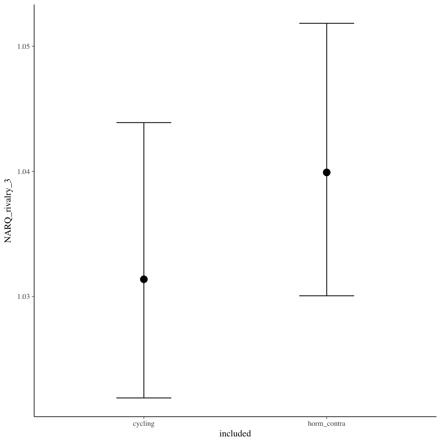
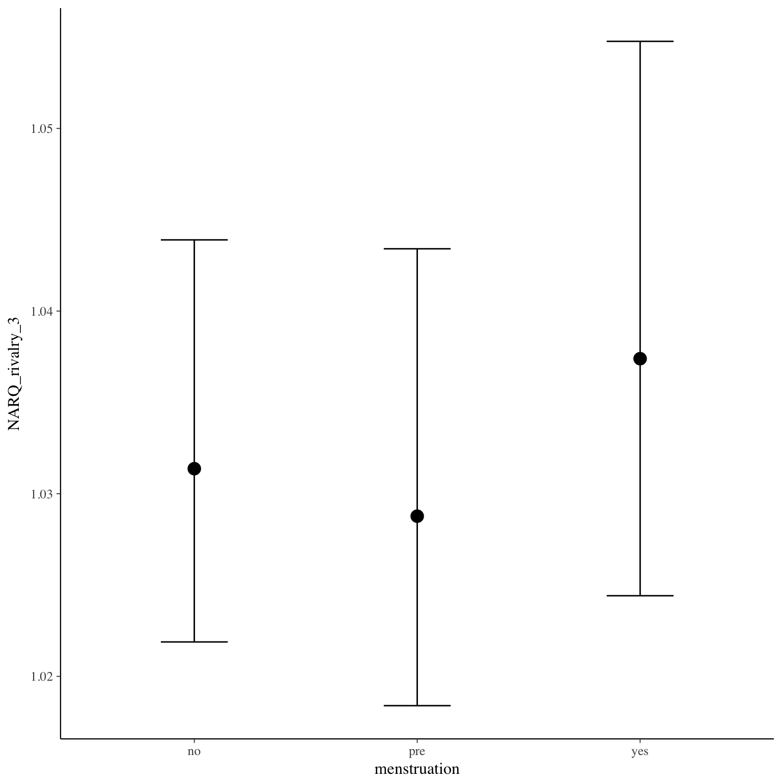
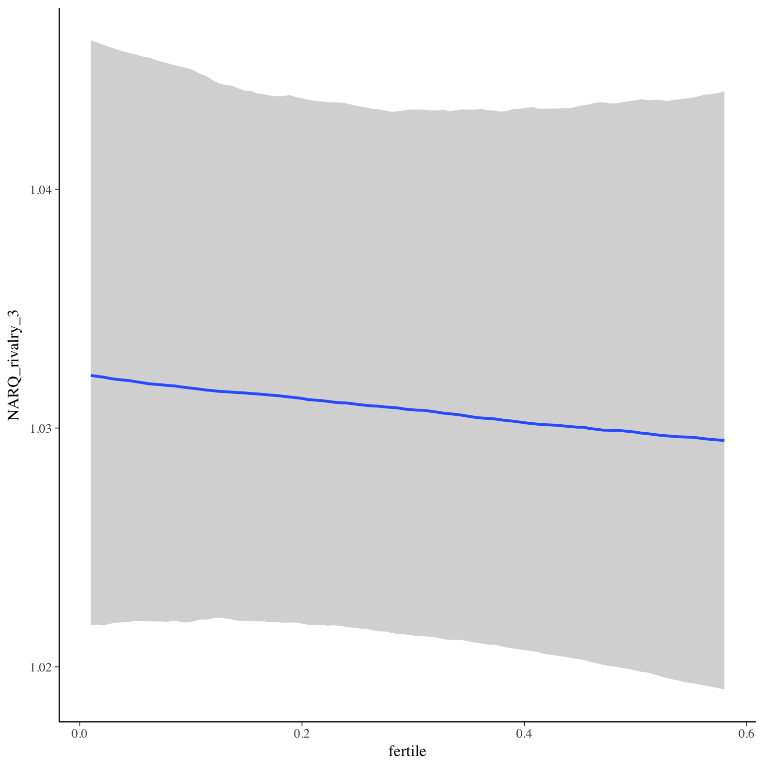
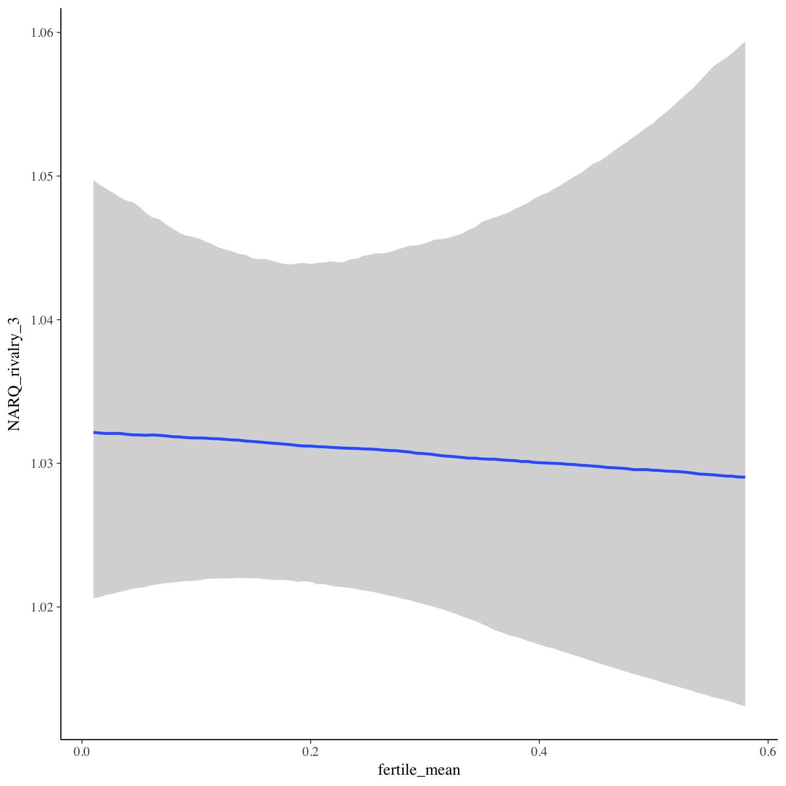
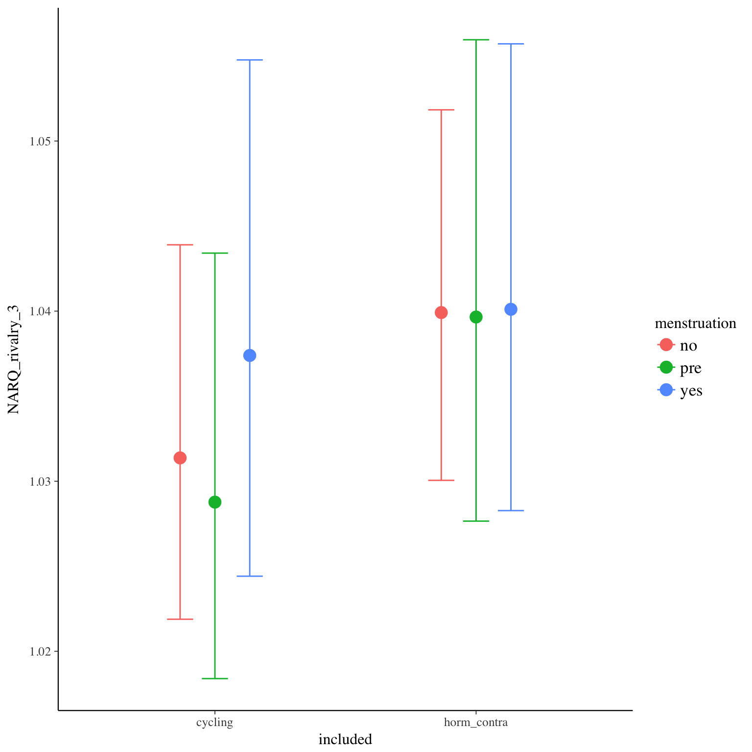
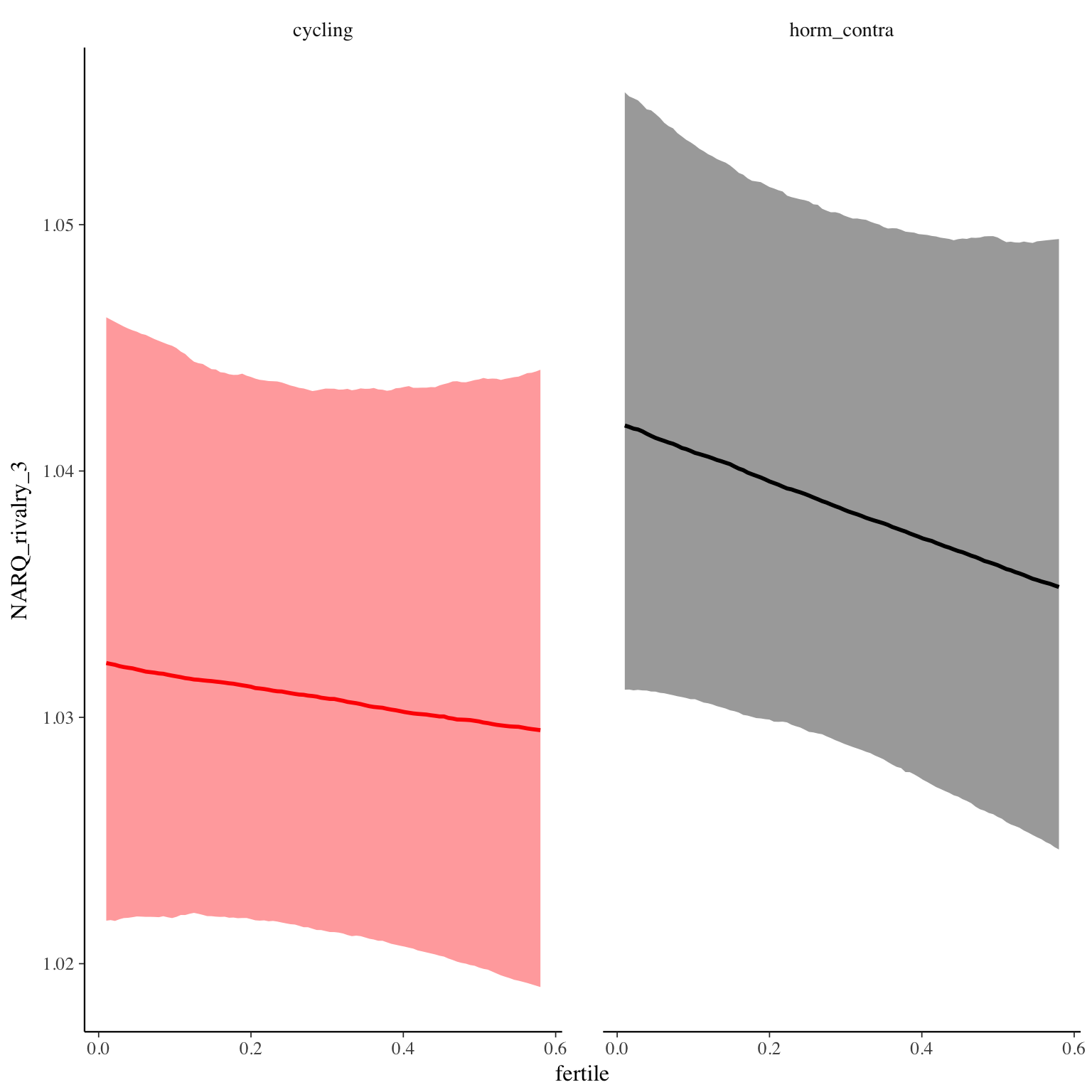
Diagnostics
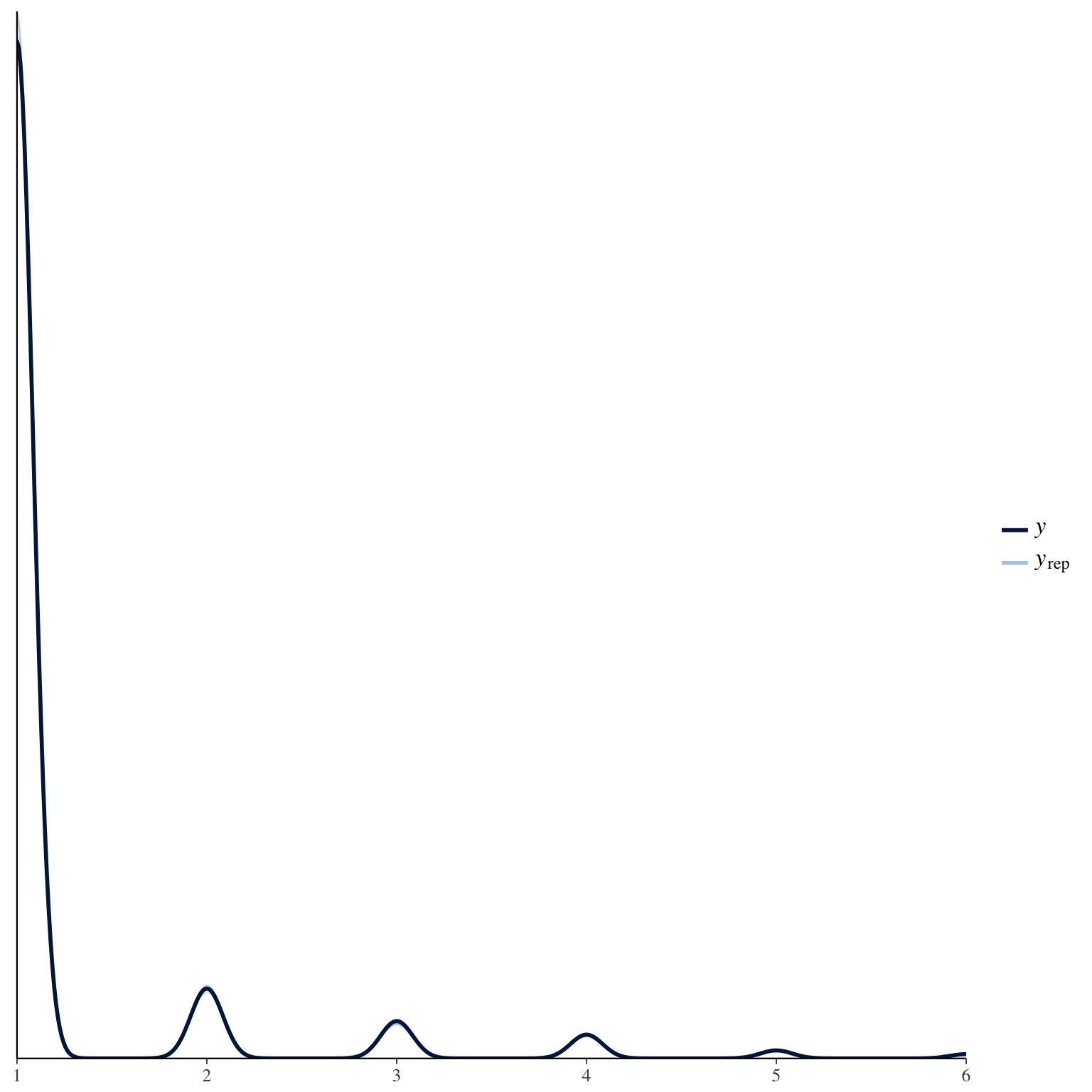
relationship_satisfaction_1
Item text:
Wie zufrieden waren Sie insgesamt seit Ihrem letzten Eintrag mit Ihrer Beziehung?
Item translation:
4. How satisfied were you with your relationship?
Choices:
| choice | value | frequency | percent |
|---|---|---|---|
| 1 | Nicht zufrieden | 707 | 0.02 |
| 2 | Überwiegend nicht zufrieden | 880 | 0.03 |
| 3 | Eher nicht zufrieden | 2189 | 0.07 |
| 4 | Eher zufrieden | 6476 | 0.22 |
| 5 | Überwiegend zufrieden | 9008 | 0.3 |
| 6 | Sehr zufrieden | 10642 | 0.36 |
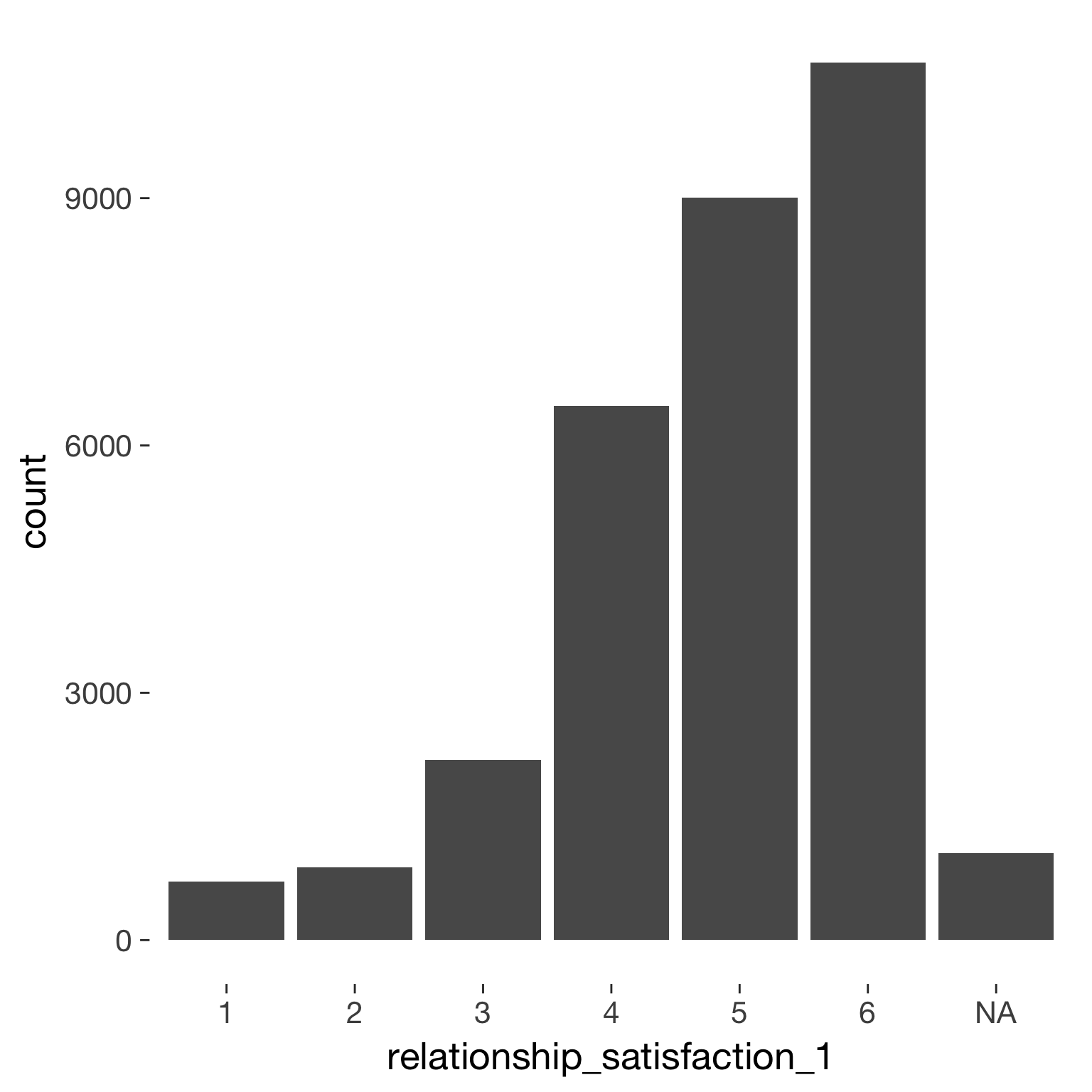
Model
Model summary
 Family: cumulative(logit)
Formula: relationship_satisfaction_1 ~ included * (menstruation + fertile) + fertile_mean + (1 + fertile + menstruation | person)
         disc = 1
   Data: diary (Number of observations: 26568)
Samples: 4 chains, each with iter = 2000; warmup = 1000; thin = 1;
         total post-warmup samples = 4000
    ICs: LOO = 69728.82; WAIC = Not computed

Group-Level Effects:
~person (Number of levels: 1043)
                                     Estimate Est.Error l-95% CI u-95% CI Eff.Sample Rhat
sd(Intercept)                            1.79      0.05     1.68     1.90        651 1.00
sd(fertile)                              1.94      0.12     1.71     2.18        843 1.00
sd(menstruationpre)                      0.97      0.06     0.85     1.09        664 1.00
sd(menstruationyes)                      0.97      0.06     0.85     1.08        870 1.01
cor(Intercept,fertile)                  -0.25      0.06    -0.36    -0.14       1573 1.00
cor(Intercept,menstruationpre)          -0.11      0.07    -0.23     0.02       1503 1.00
cor(fertile,menstruationpre)             0.38      0.07     0.24     0.51        615 1.00
cor(Intercept,menstruationyes)          -0.13      0.06    -0.25     0.00       1371 1.00
cor(fertile,menstruationyes)             0.33      0.08     0.18     0.47        591 1.01
cor(menstruationpre,menstruationyes)     0.40      0.07     0.25     0.53        568 1.01

Population-Level Effects:
                                    Estimate Est.Error l-95% CI u-95% CI Eff.Sample Rhat
Intercept[1]                           -4.97      0.15    -5.28    -4.69        720 1.00
Intercept[2]                           -3.89      0.14    -4.17    -3.61        685 1.00
Intercept[3]                           -2.60      0.14    -2.88    -2.32        664 1.00
Intercept[4]                           -1.09      0.14    -1.38    -0.82        658 1.00
Intercept[5]                           -0.77      0.14    -1.05    -0.50        657 1.00
Intercept[6]                            1.08      0.14     0.80     1.35        654 1.00
includedhorm_contra                     0.35      0.12     0.11     0.59        423 1.01
menstruationpre                         0.08      0.08    -0.07     0.24       1493 1.00
menstruationyes                         0.08      0.08    -0.07     0.23       1534 1.00
fertile                                 0.02      0.16    -0.29     0.33       1591 1.00
fertile_mean                           -0.51      0.60    -1.72     0.66       1292 1.00
includedhorm_contra:menstruationpre    -0.09      0.10    -0.29     0.10       1493 1.00
includedhorm_contra:menstruationyes     0.02      0.10    -0.18     0.22       1532 1.00
includedhorm_contra:fertile            -0.23      0.20    -0.63     0.16       1499 1.00

Samples were drawn using sampling(NUTS). For each parameter, Eff.Sample
is a crude measure of effective sample size, and Rhat is the potential
scale reduction factor on split chains (at convergence, Rhat = 1).
Coefficient plot
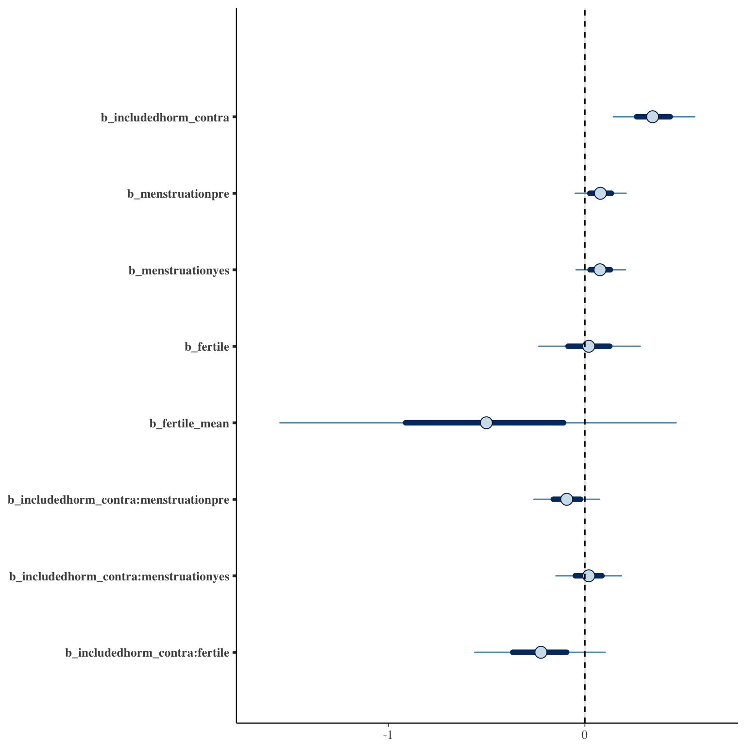
Marginal effect plots
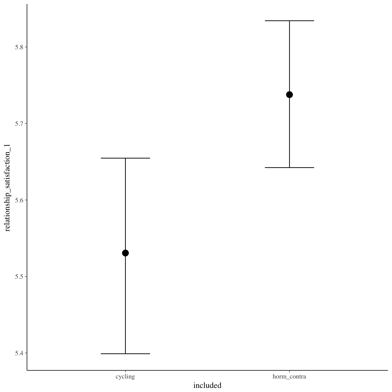
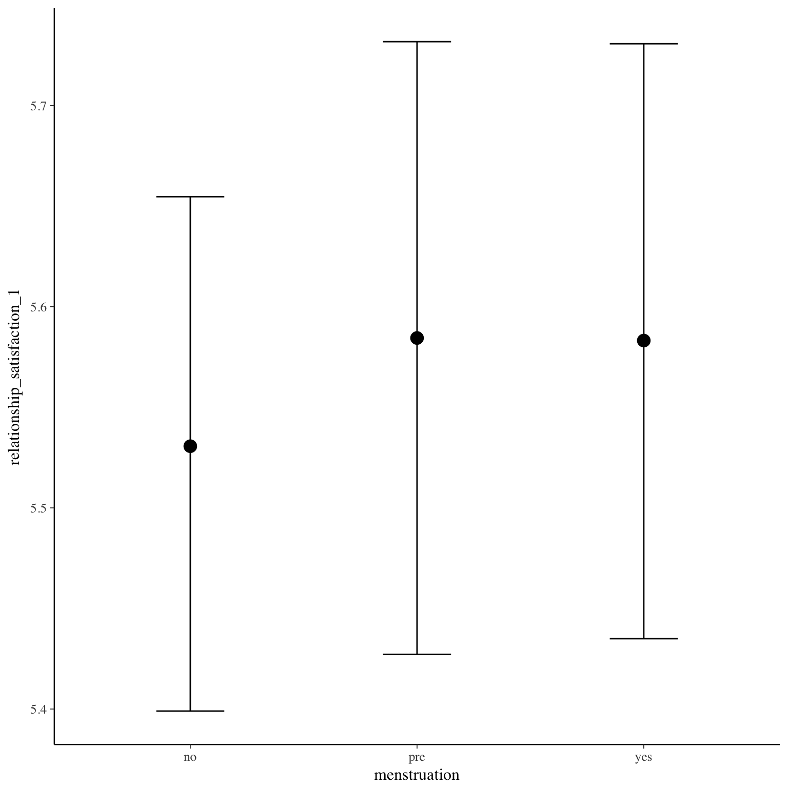
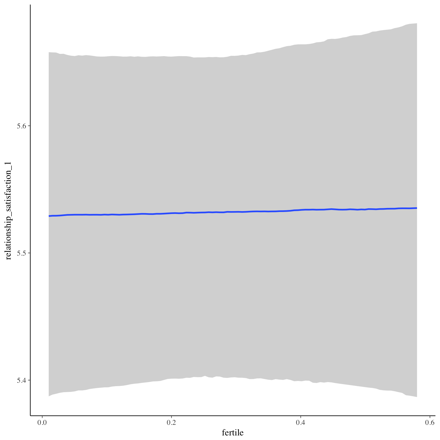
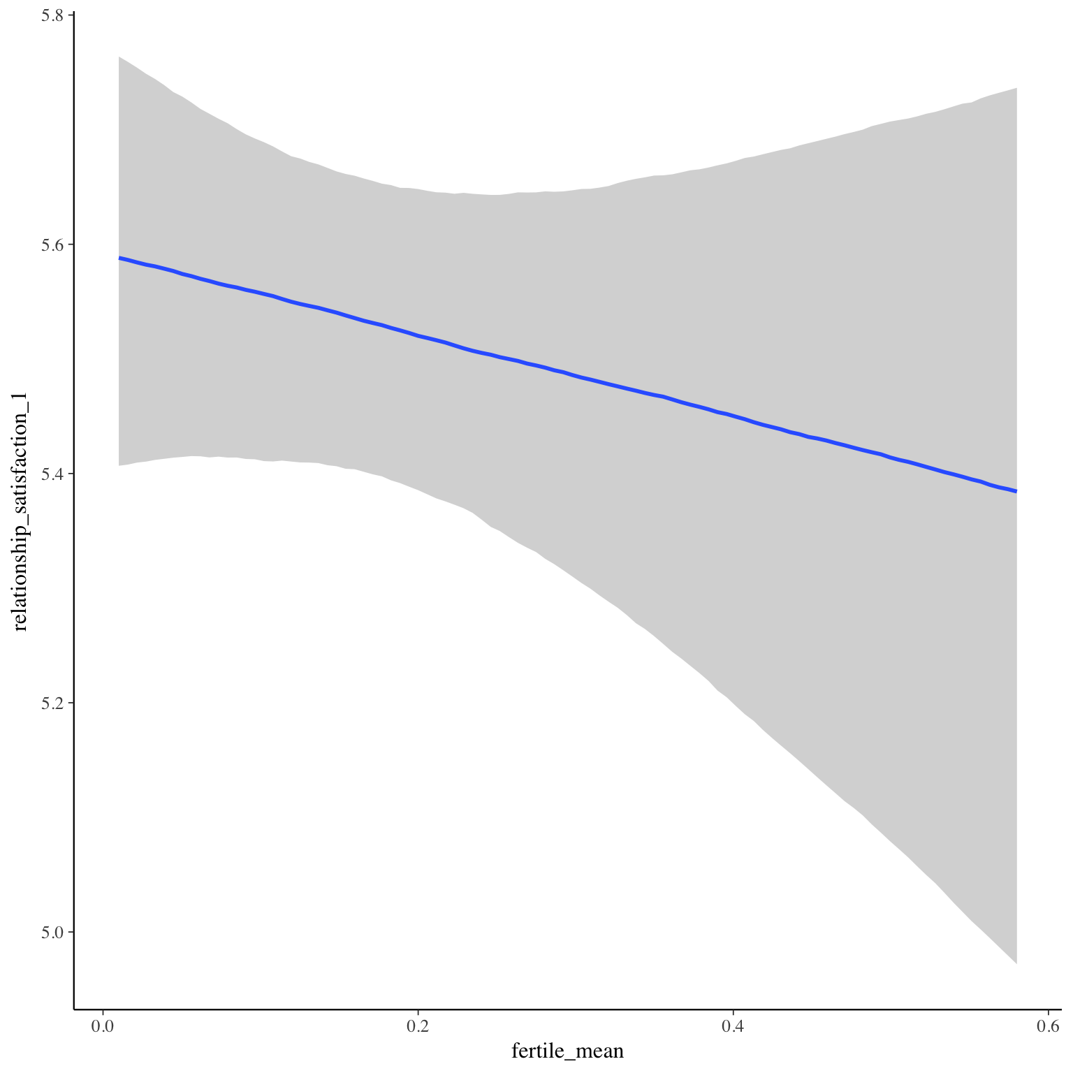
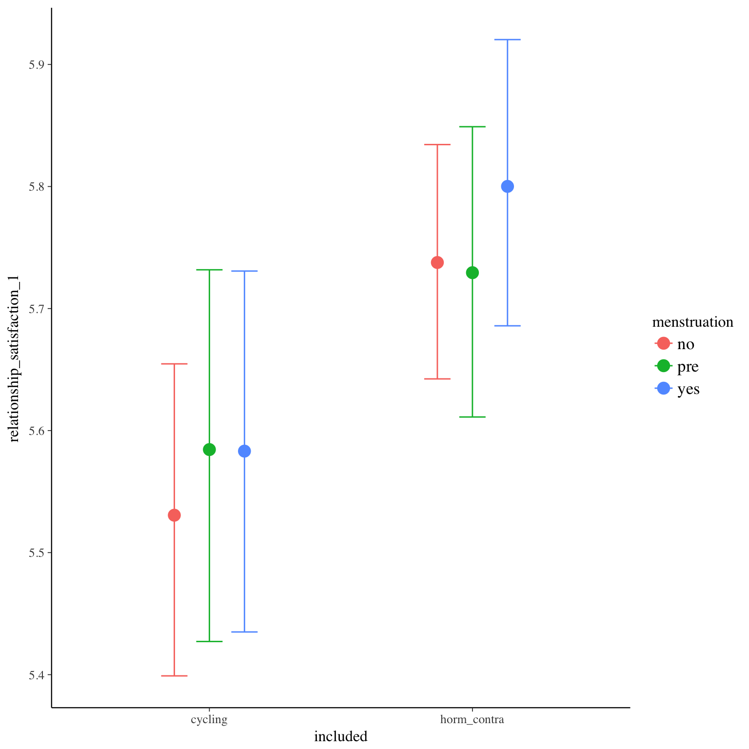
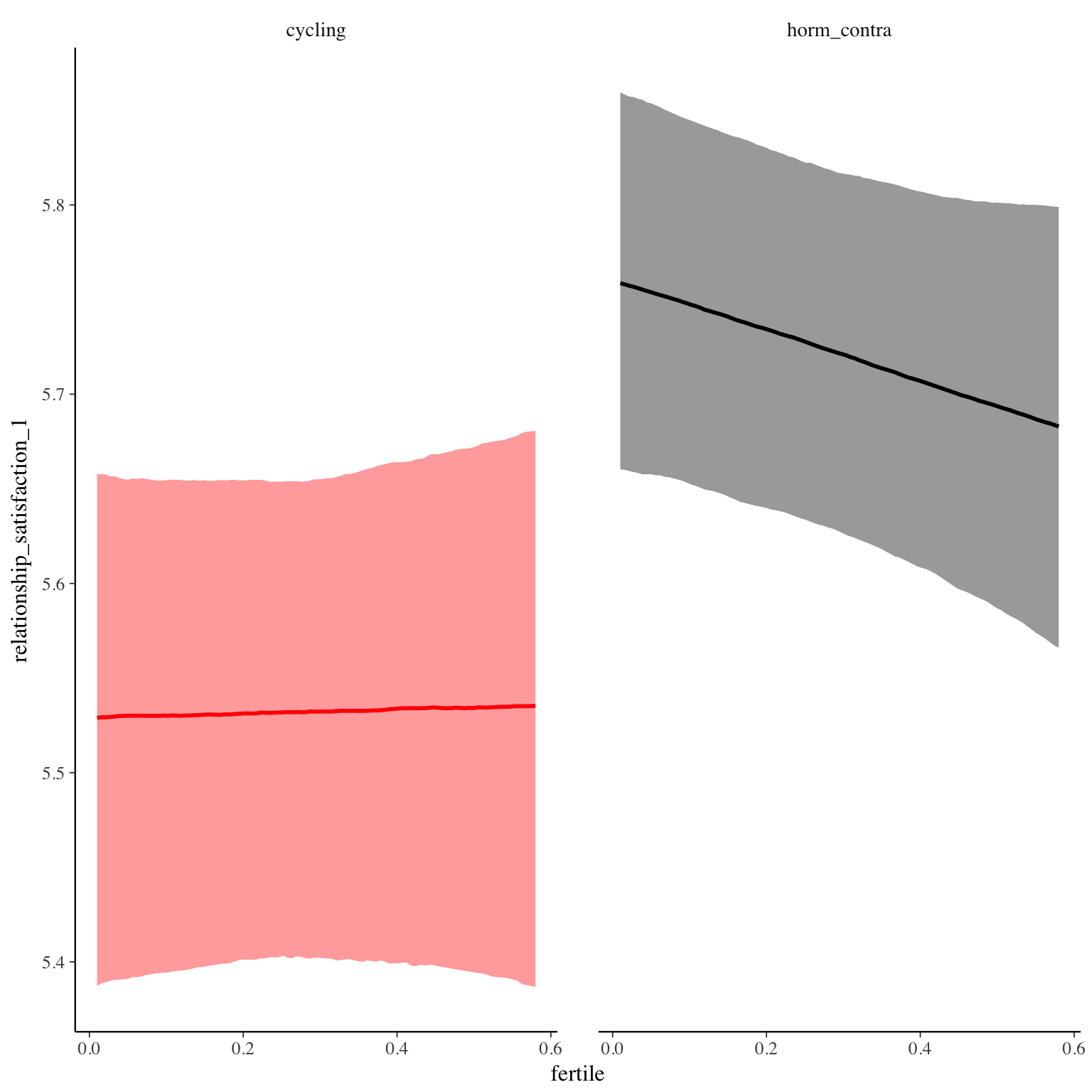
Diagnostics
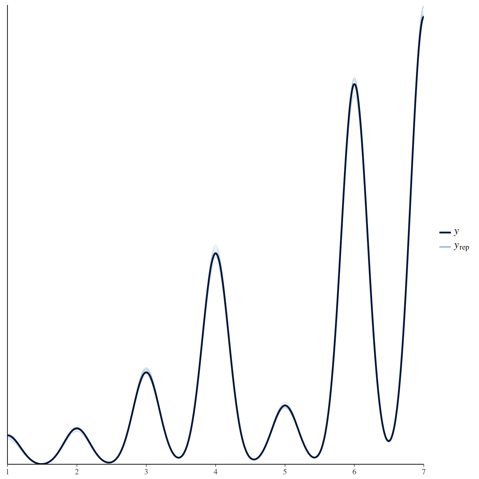
self_esteem_1
Item text:
… war ich im Großen und Ganzen zufrieden mit mir selbst.
Item translation:
24. On the whole, I was satisfied with myself (based on Rosenberg, 1965).
Choices:
| choice | value | frequency | percent |
|---|---|---|---|
| 1 | Stimme nicht zu | 1115 | 0.04 |
| 2 | Stimme überwiegend nicht zu | 1290 | 0.04 |
| 3 | Stimme eher nicht zu | 3612 | 0.12 |
| 4 | Stimme eher zu | 9965 | 0.33 |
| 5 | Stimme überwiegend zu | 9971 | 0.33 |
| 6 | Stimme voll zu | 3928 | 0.13 |
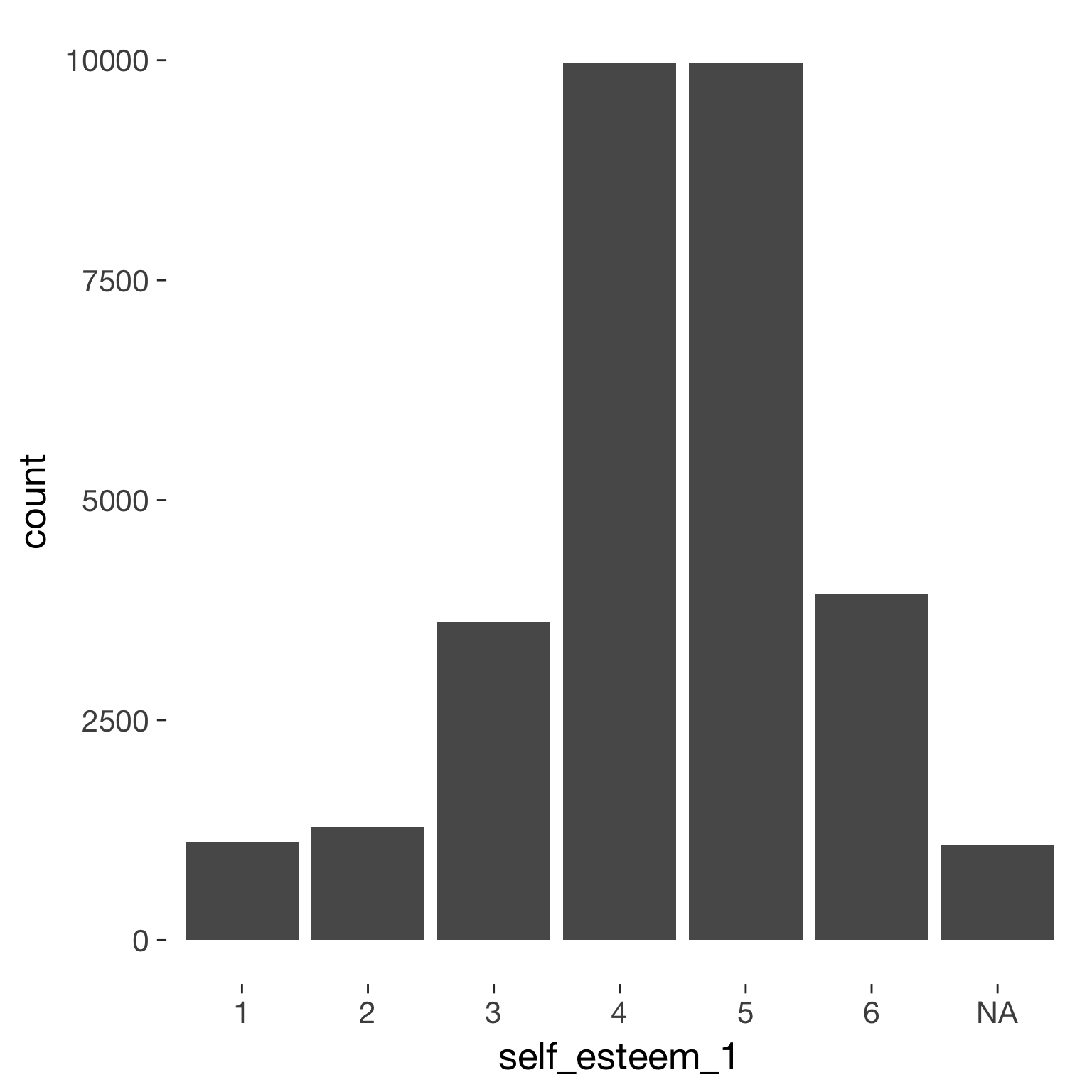
Model
Model summary
 Family: cumulative(logit)
Formula: self_esteem_1 ~ included * (menstruation + fertile) + fertile_mean + (1 + fertile + menstruation | person)
         disc = 1
   Data: diary (Number of observations: 26549)
Samples: 4 chains, each with iter = 2000; warmup = 1000; thin = 1;
         total post-warmup samples = 4000
    ICs: LOO = 64765.31; WAIC = Not computed

Group-Level Effects:
~person (Number of levels: 1043)
                                     Estimate Est.Error l-95% CI u-95% CI Eff.Sample Rhat
sd(Intercept)                            1.92      0.05     1.82     2.03        640    1
sd(fertile)                              1.80      0.11     1.58     2.02        967    1
sd(menstruationpre)                      0.71      0.06     0.59     0.83        754    1
sd(menstruationyes)                      0.68      0.06     0.56     0.80        862    1
cor(Intercept,fertile)                  -0.32      0.05    -0.42    -0.21       2181    1
cor(Intercept,menstruationpre)          -0.31      0.06    -0.42    -0.18       2704    1
cor(fertile,menstruationpre)             0.40      0.08     0.23     0.56        750    1
cor(Intercept,menstruationyes)          -0.21      0.07    -0.34    -0.07       2485    1
cor(fertile,menstruationyes)             0.29      0.09     0.10     0.46        800    1
cor(menstruationpre,menstruationyes)     0.59      0.09     0.40     0.76        513    1

Population-Level Effects:
                                    Estimate Est.Error l-95% CI u-95% CI Eff.Sample Rhat
Intercept[1]                           -4.80      0.15    -5.10    -4.51        671 1.00
Intercept[2]                           -3.63      0.14    -3.91    -3.35        636 1.00
Intercept[3]                           -2.15      0.14    -2.44    -1.87        630 1.00
Intercept[4]                            0.11      0.14    -0.18     0.38        620 1.00
Intercept[5]                            2.79      0.14     2.50     3.06        622 1.00
includedhorm_contra                    -0.08      0.13    -0.34     0.15        356 1.02
menstruationpre                        -0.13      0.07    -0.26     0.01       1854 1.00
menstruationyes                        -0.24      0.07    -0.37    -0.11       2082 1.00
fertile                                -0.12      0.15    -0.41     0.19       1836 1.00
fertile_mean                           -0.22      0.59    -1.38     0.90       1166 1.00
includedhorm_contra:menstruationpre     0.10      0.09    -0.08     0.28       1868 1.00
includedhorm_contra:menstruationyes     0.22      0.09     0.04     0.40       1857 1.00
includedhorm_contra:fertile             0.21      0.19    -0.18     0.59       1763 1.00

Samples were drawn using sampling(NUTS). For each parameter, Eff.Sample
is a crude measure of effective sample size, and Rhat is the potential
scale reduction factor on split chains (at convergence, Rhat = 1).
Coefficient plot
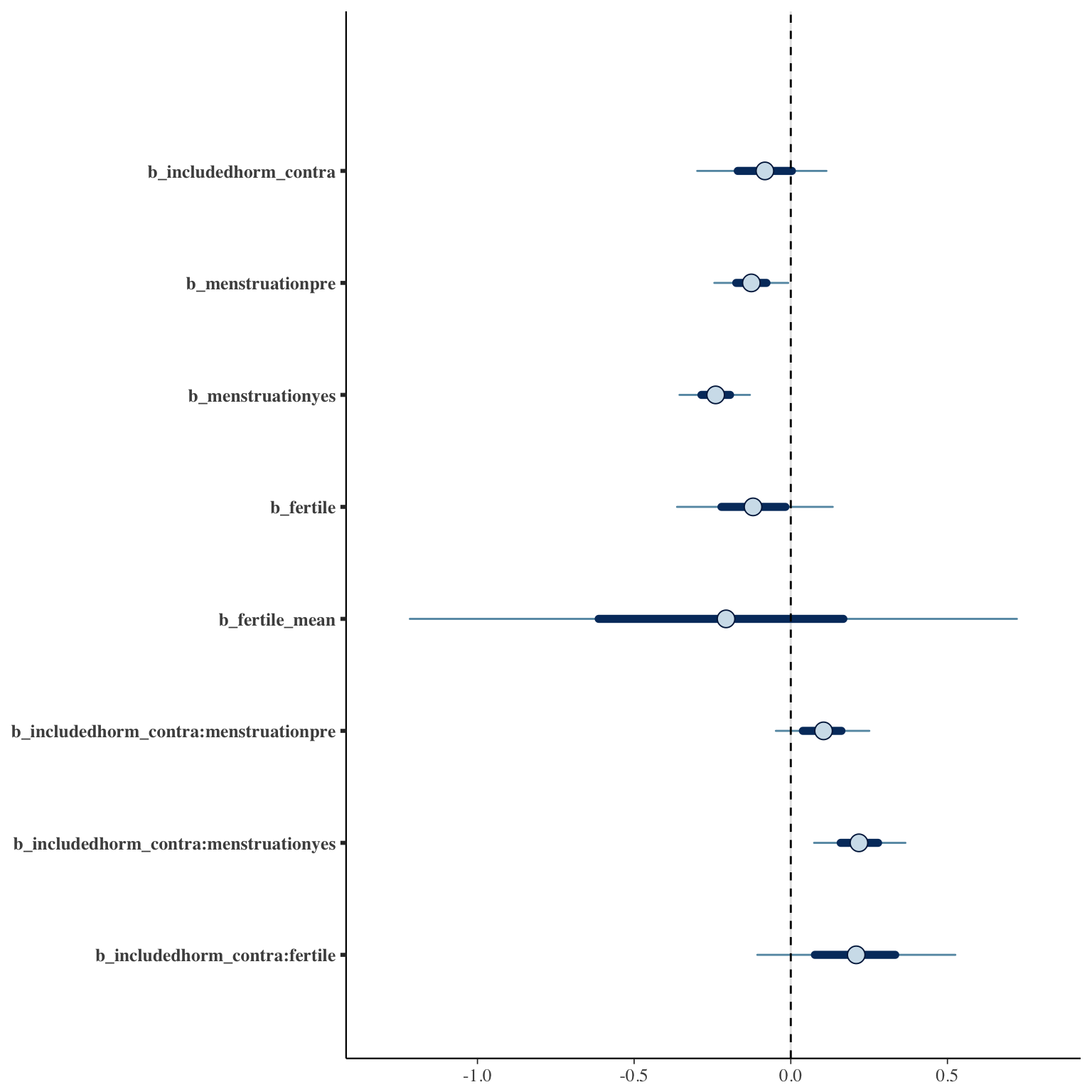
Marginal effect plots
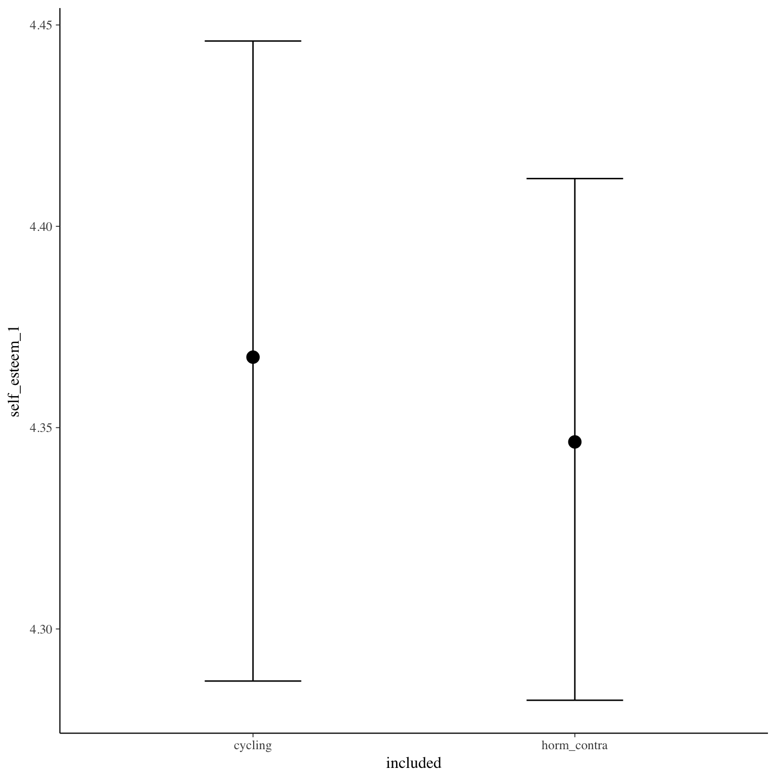
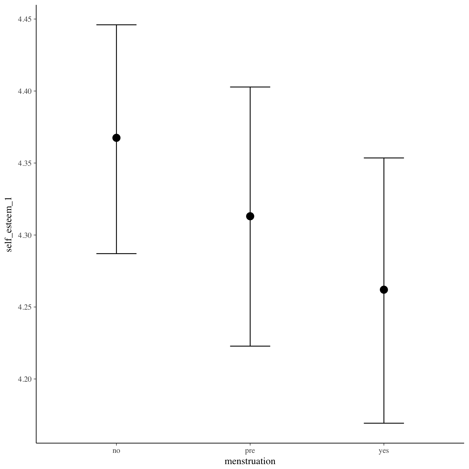
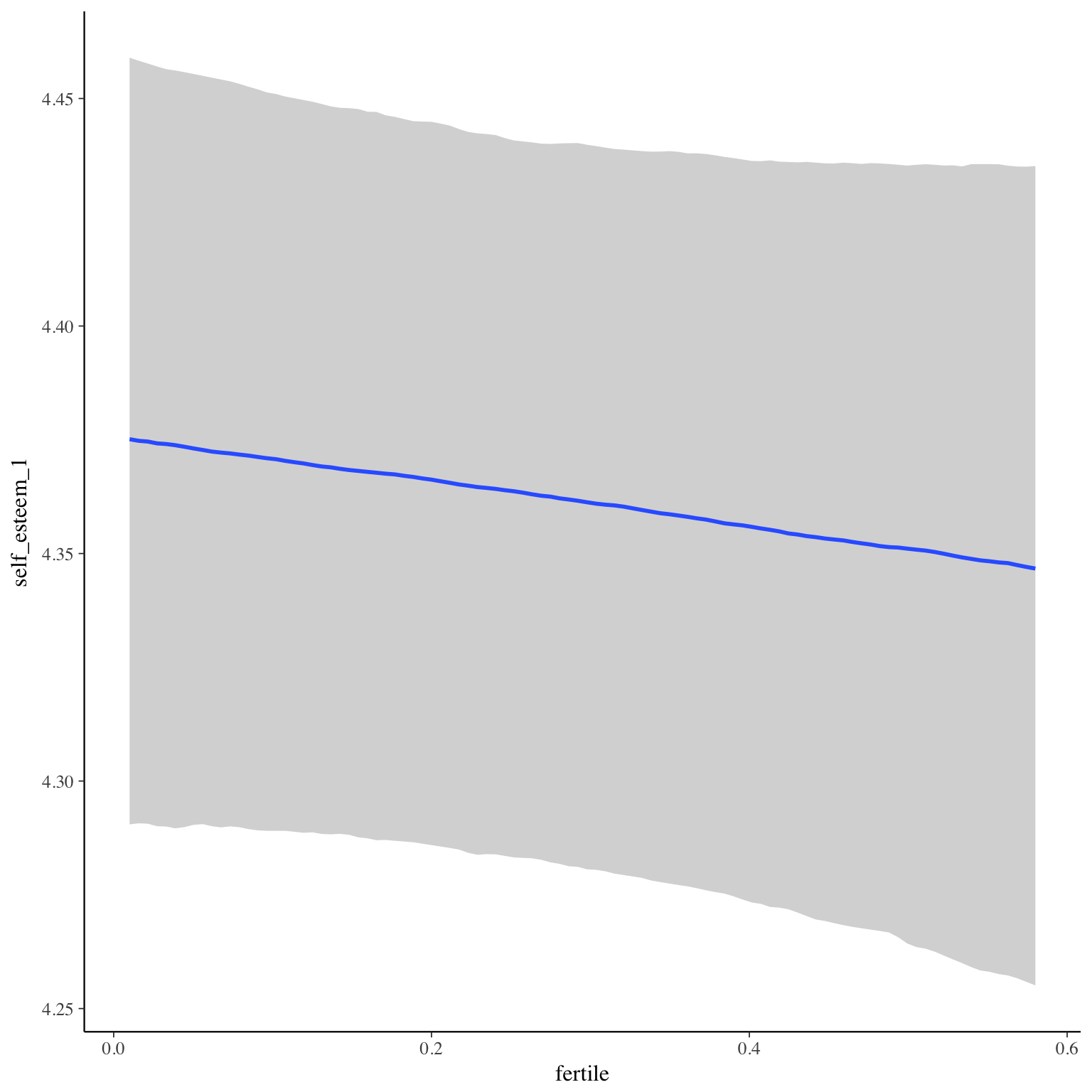
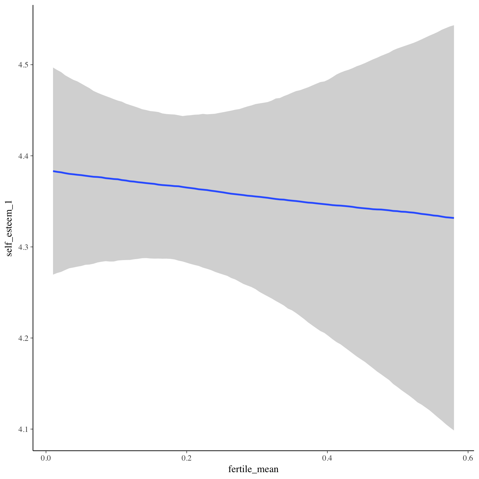
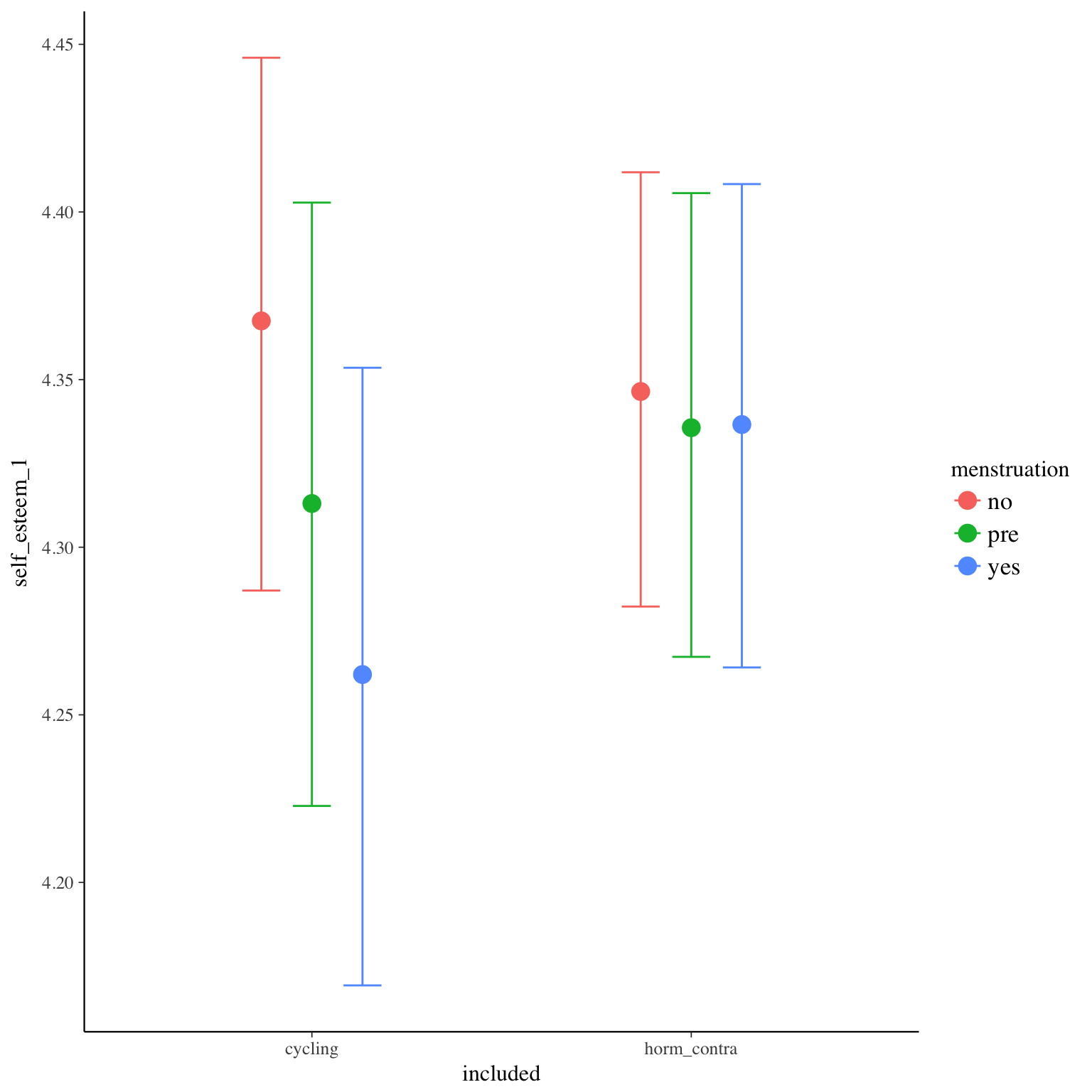
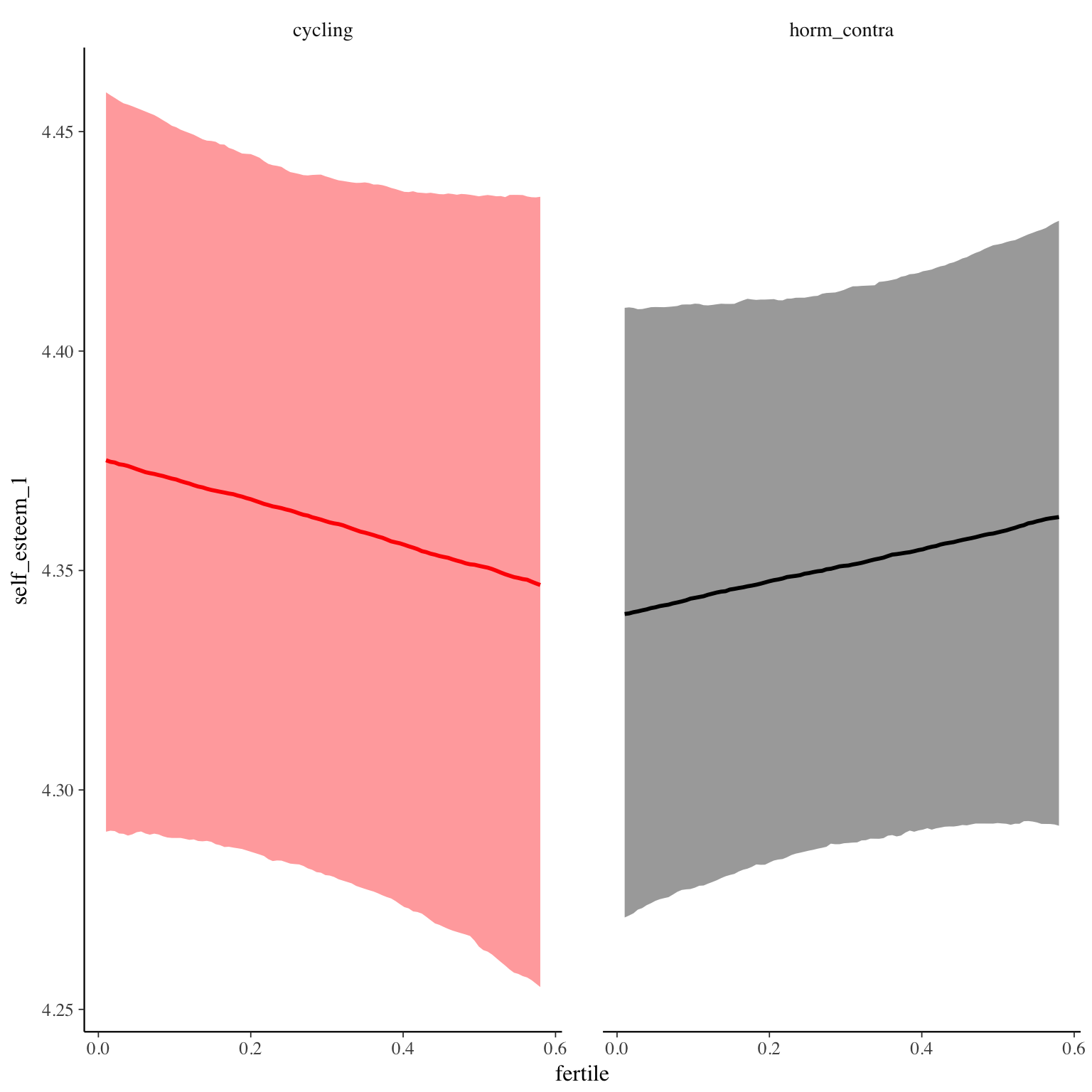
Diagnostics
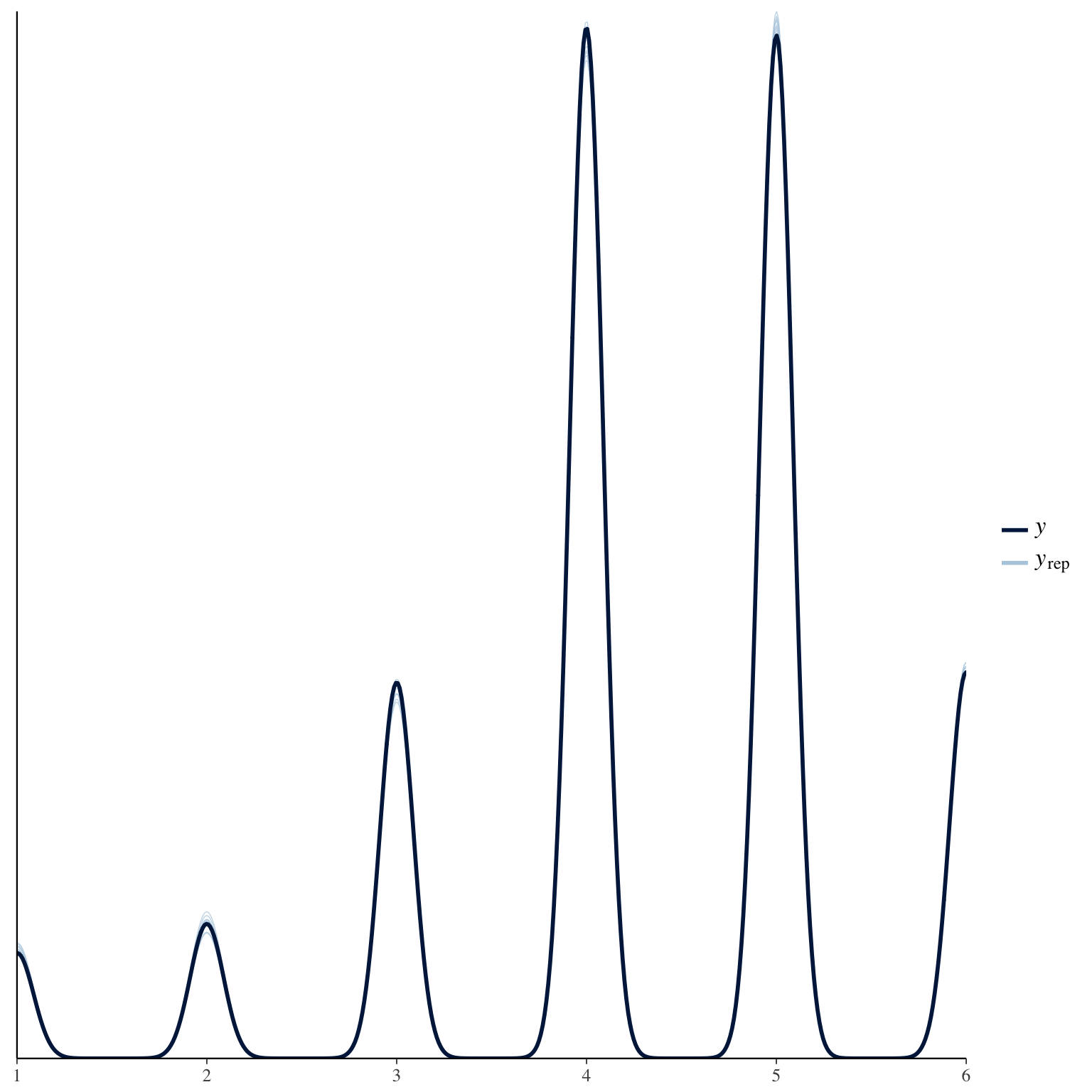
sexual_intercourse_1
Item text:
Wie sehr hatten Sie seit Ihrem letzten Eintrag Lust, mit Ihrem Partner Geschlechtsverkehr zu haben?
Item translation:
6. How much were you in the mood to have sex with your partner?
Choices:
| choice | value | frequency | percent |
|---|---|---|---|
| 1 | gar nicht | 3780 | 0.13 |
| 2 | kaum | 5133 | 0.17 |
| 3 | etwas | 9262 | 0.31 |
| 4 | viel | 7492 | 0.25 |
| 5 | sehr viel | 4235 | 0.14 |
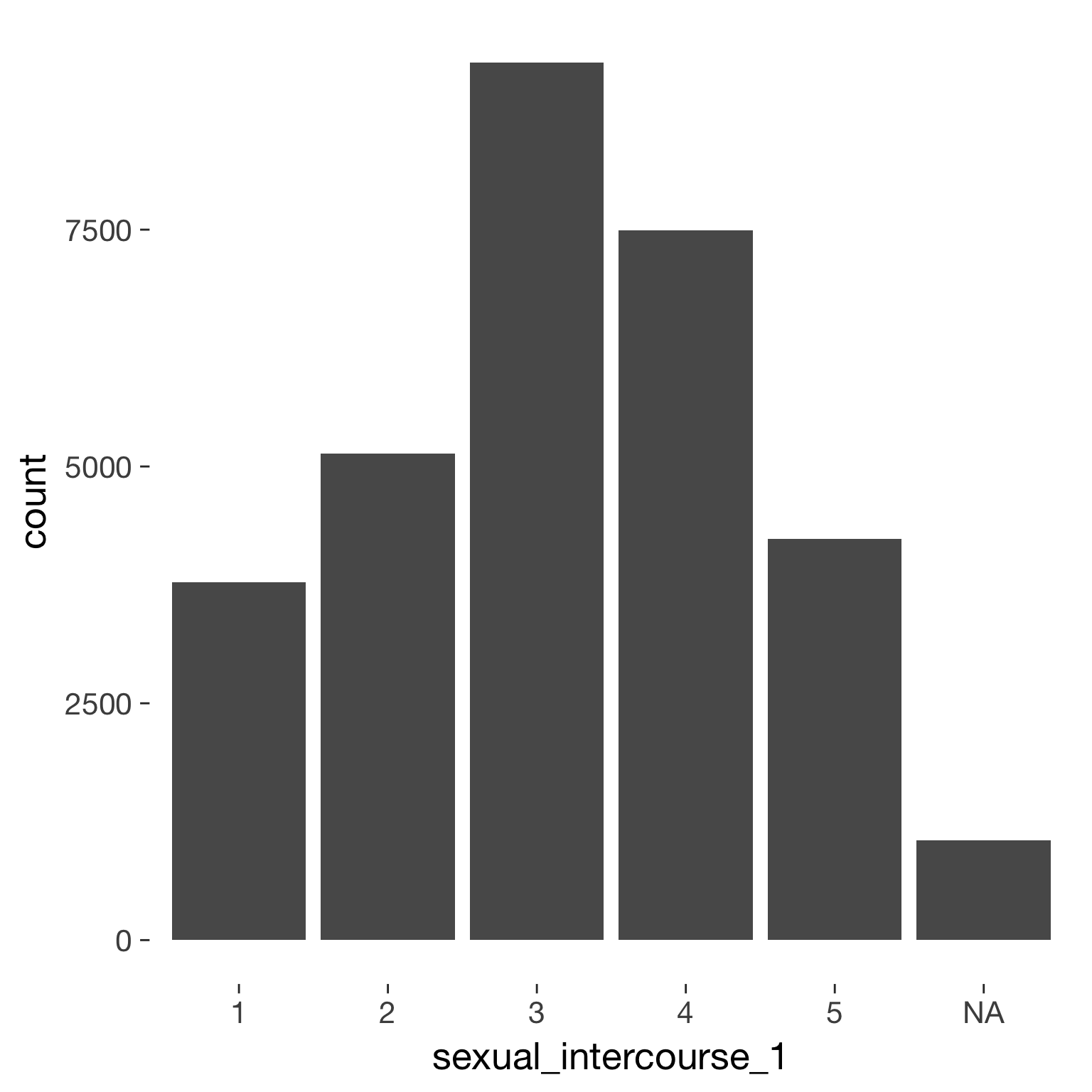
Model
Model summary
 Family: cumulative(logit)
Formula: sexual_intercourse_1 ~ included * (menstruation + fertile) + fertile_mean + (1 + fertile + menstruation | person)
         disc = 1
   Data: diary (Number of observations: 26568)
Samples: 4 chains, each with iter = 2000; warmup = 1000; thin = 1;
         total post-warmup samples = 4000
    ICs: LOO = 70553.56; WAIC = Not computed

Group-Level Effects:
~person (Number of levels: 1043)
                                     Estimate Est.Error l-95% CI u-95% CI Eff.Sample Rhat
sd(Intercept)                            1.58      0.05     1.49     1.68        848 1.00
sd(fertile)                              1.80      0.11     1.59     2.02        862 1.01
sd(menstruationpre)                      0.83      0.06     0.71     0.94        758 1.00
sd(menstruationyes)                      0.95      0.06     0.85     1.06        744 1.00
cor(Intercept,fertile)                  -0.26      0.06    -0.37    -0.14       1784 1.00
cor(Intercept,menstruationpre)          -0.13      0.07    -0.25     0.00       1702 1.00
cor(fertile,menstruationpre)             0.31      0.08     0.15     0.45        690 1.01
cor(Intercept,menstruationyes)          -0.18      0.06    -0.29    -0.06       1422 1.00
cor(fertile,menstruationyes)             0.20      0.08     0.04     0.35        589 1.01
cor(menstruationpre,menstruationyes)     0.13      0.08    -0.04     0.28        489 1.00

Population-Level Effects:
                                    Estimate Est.Error l-95% CI u-95% CI Eff.Sample Rhat
Intercept[1]                           -2.34      0.13    -2.58    -2.09        835 1.00
Intercept[2]                           -0.83      0.13    -1.08    -0.58        834 1.00
Intercept[3]                            0.99      0.13     0.74     1.24        844 1.00
Intercept[4]                            2.82      0.13     2.58     3.08        859 1.00
includedhorm_contra                     0.63      0.11     0.41     0.85        527 1.01
menstruationpre                        -0.15      0.07    -0.29     0.00       1773 1.00
menstruationyes                        -0.43      0.08    -0.58    -0.27       1626 1.00
fertile                                 0.57      0.15     0.26     0.87       1663 1.00
fertile_mean                            0.27      0.55    -0.77     1.33       1091 1.00
includedhorm_contra:menstruationpre     0.01      0.10    -0.18     0.20       1810 1.00
includedhorm_contra:menstruationyes     0.16      0.10    -0.04     0.35       1661 1.00
includedhorm_contra:fertile            -0.89      0.20    -1.28    -0.50       1661 1.00

Samples were drawn using sampling(NUTS). For each parameter, Eff.Sample
is a crude measure of effective sample size, and Rhat is the potential
scale reduction factor on split chains (at convergence, Rhat = 1).
Coefficient plot
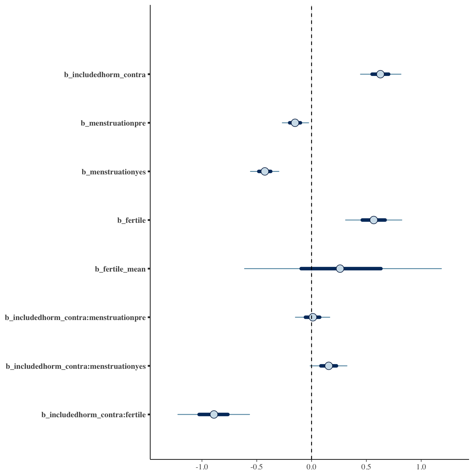
Marginal effect plots
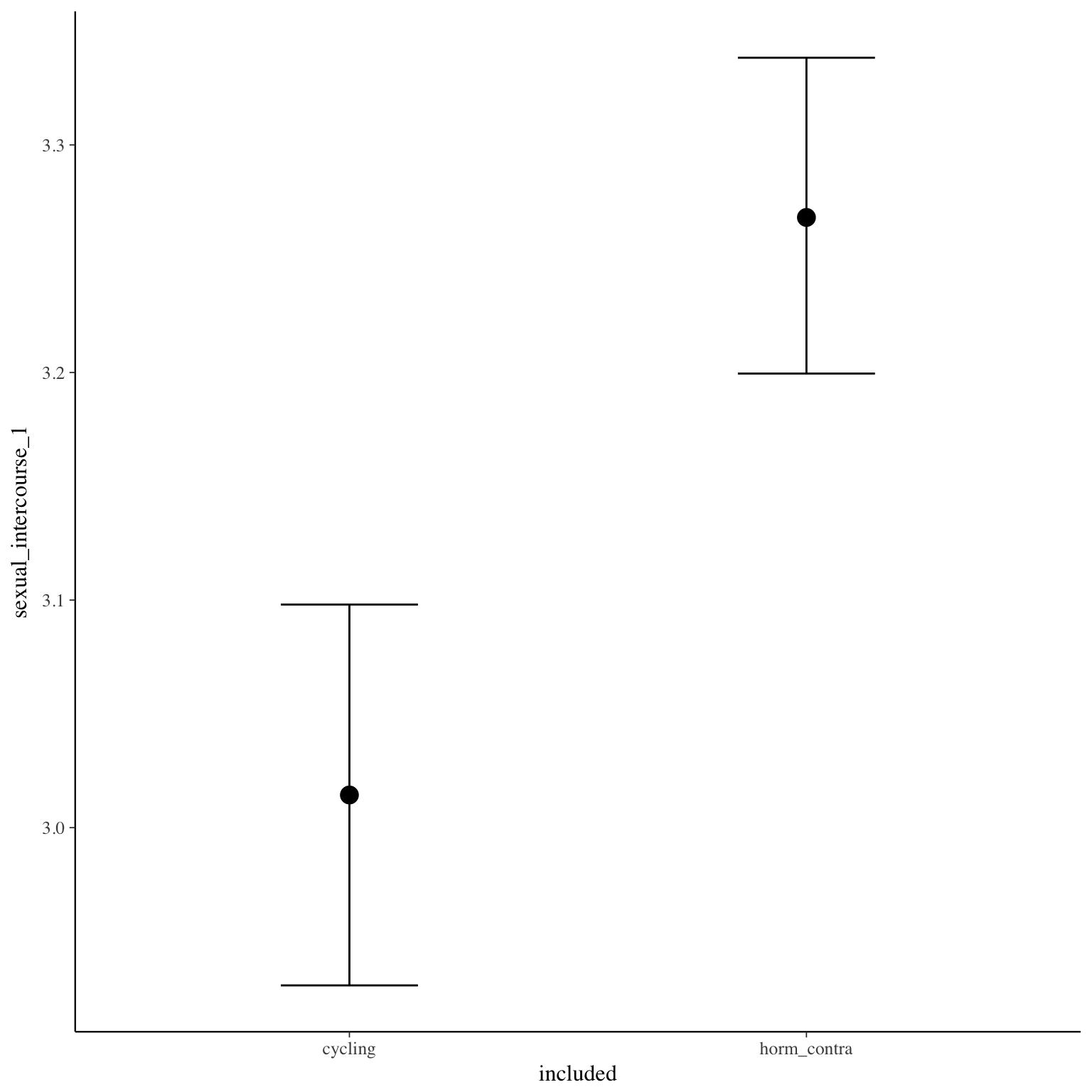
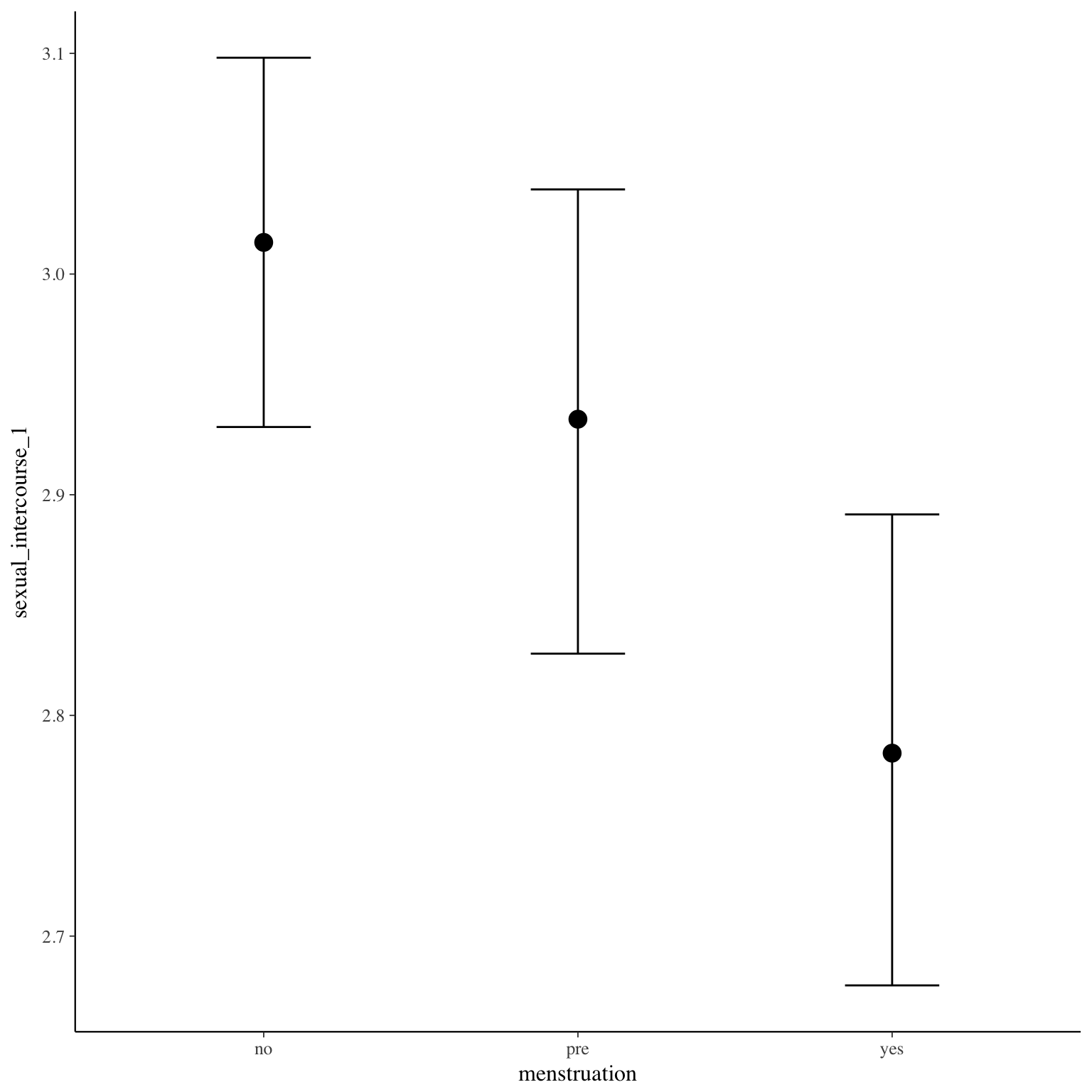
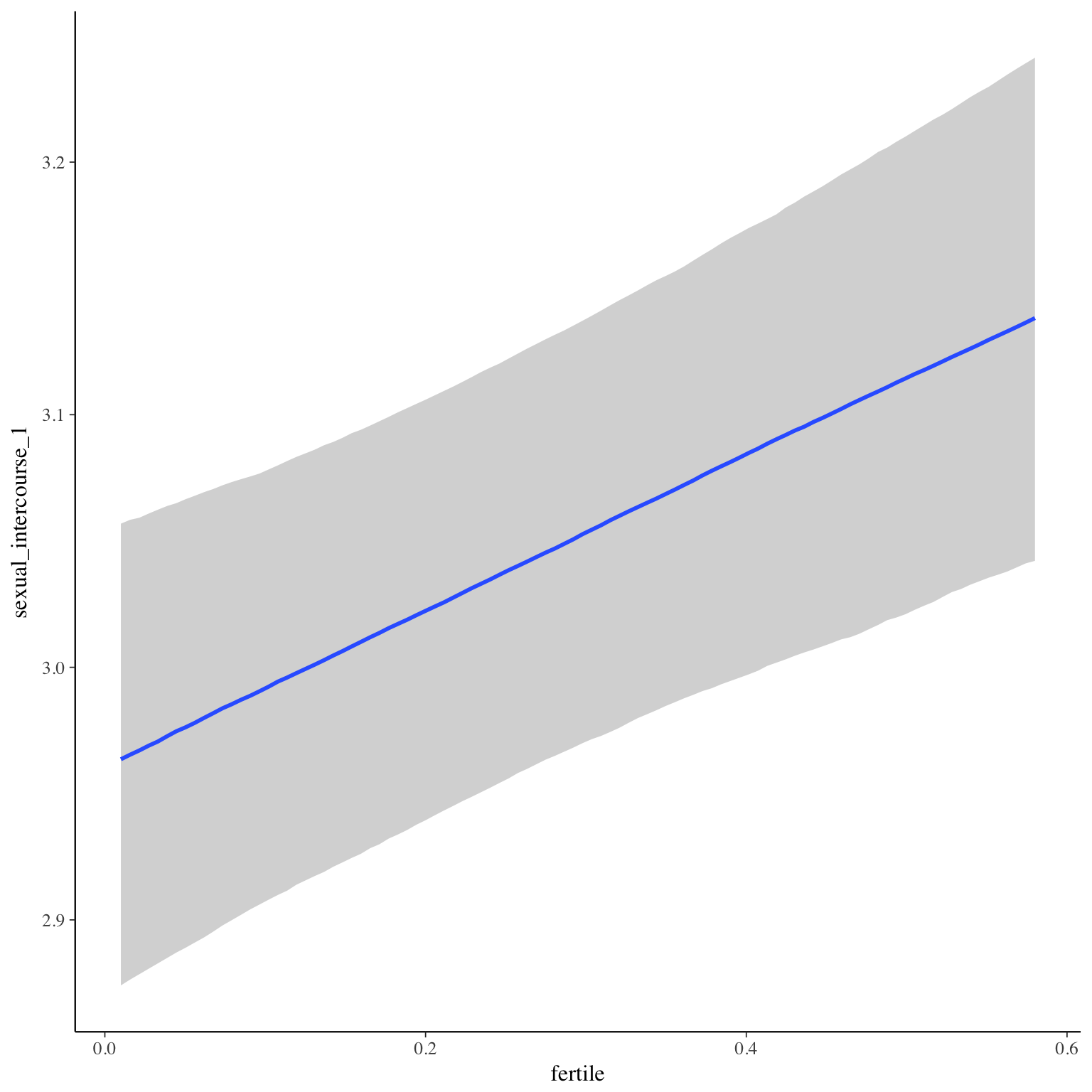
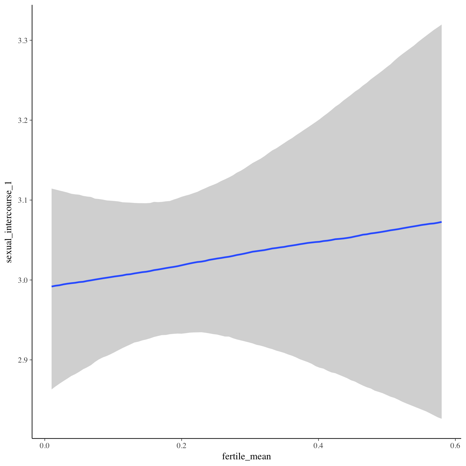
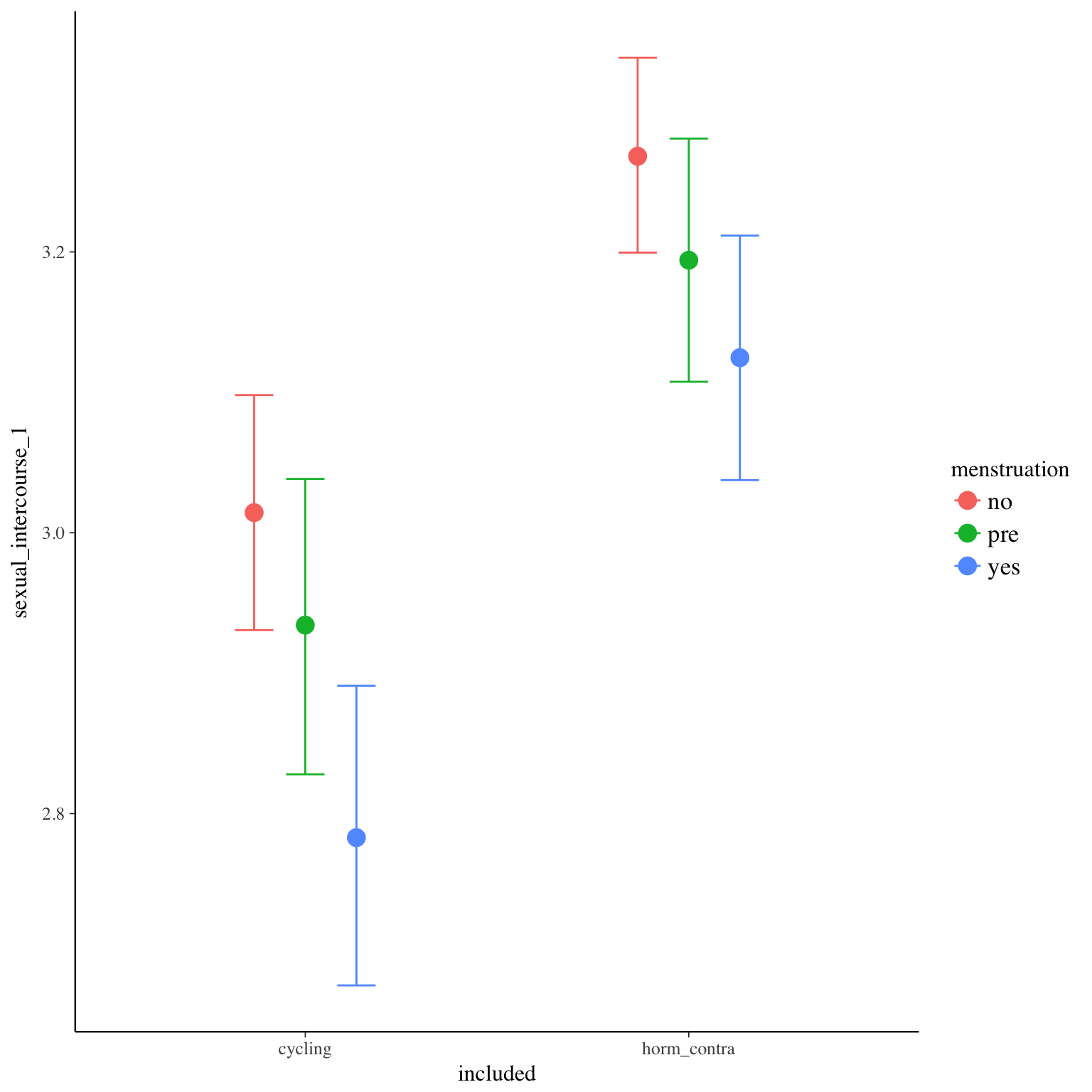
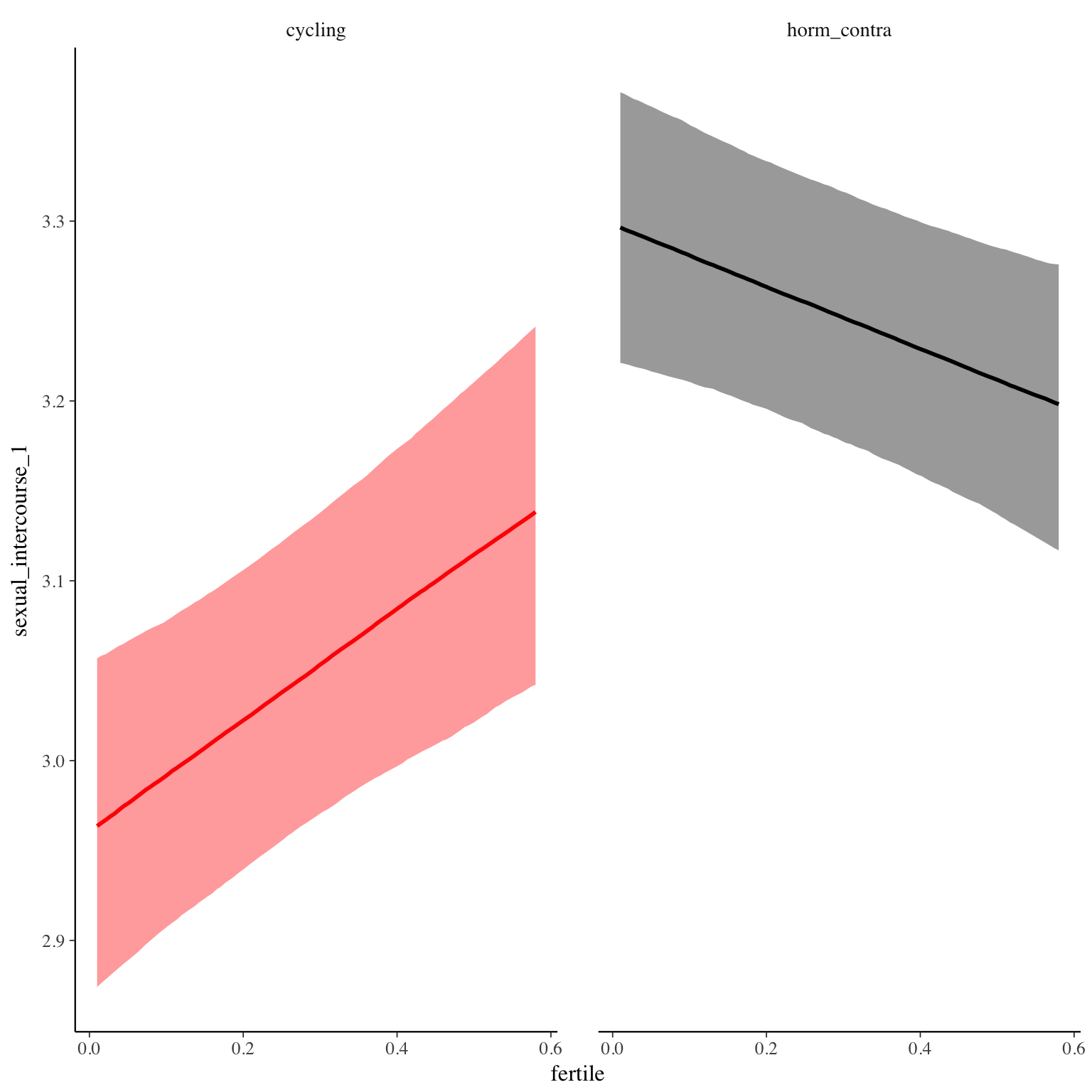
Diagnostics
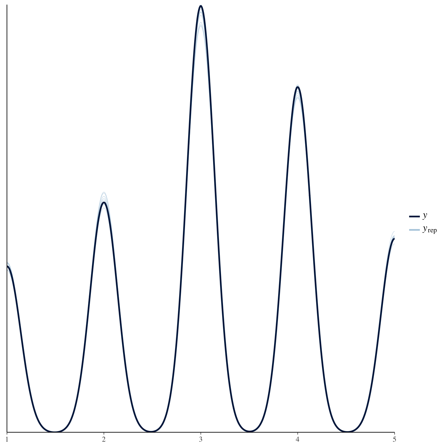
sexual_intercourse_2
Item text:
Hatten Sie seit Ihrem letzten Eintrag mit Ihrem Partner Geschlechtsverkehr?
Item translation:
7. Did you have sexual intercourse with your partner?
Choices:
| choice | value | frequency | percent |
|---|---|---|---|
| 0 | NA | 23389 | 0.78 |
| 1 | ja (1x) | 4485 | 0.15 |
| 2 | ja (mehrfach) | 2028 | 0.07 |
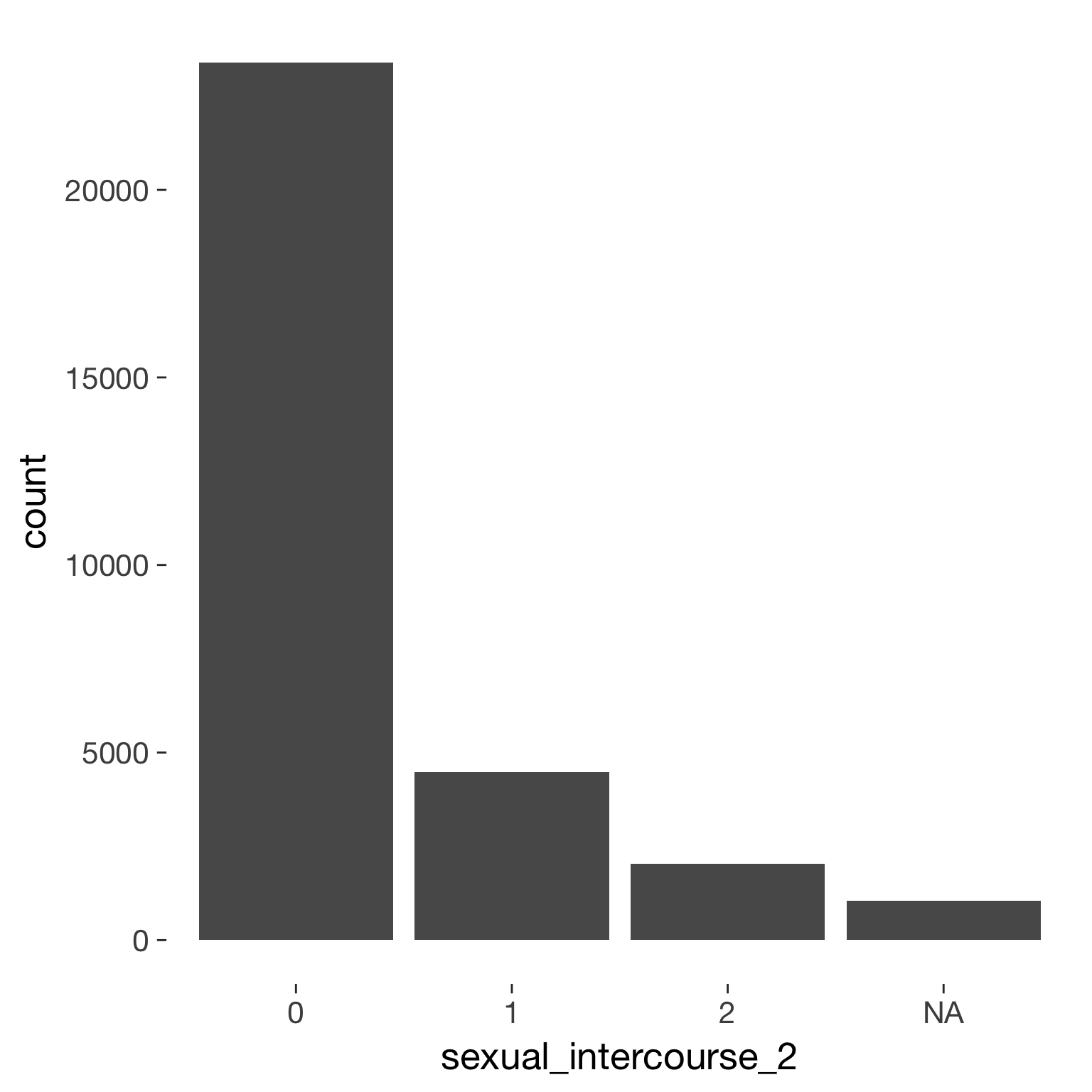
Model
Model summary
 Family: cumulative(logit)
Formula: sexual_intercourse_2 ~ included * (menstruation + fertile) + fertile_mean + (1 + fertile + menstruation | person)
         disc = 1
   Data: diary (Number of observations: 26568)
Samples: 4 chains, each with iter = 2000; warmup = 1000; thin = 1;
         total post-warmup samples = 4000
    ICs: LOO = 31568.87; WAIC = Not computed

Group-Level Effects:
~person (Number of levels: 1043)
                                     Estimate Est.Error l-95% CI u-95% CI Eff.Sample Rhat
sd(Intercept)                            1.06      0.05     0.96     1.16        693 1.01
sd(fertile)                              1.06      0.21     0.61     1.46        133 1.03
sd(menstruationpre)                      0.54      0.12     0.30     0.75        216 1.02
sd(menstruationyes)                      1.02      0.11     0.80     1.24        595 1.00
cor(Intercept,fertile)                  -0.26      0.14    -0.50     0.04        575 1.01
cor(Intercept,menstruationpre)          -0.19      0.14    -0.43     0.10        634 1.01
cor(fertile,menstruationpre)             0.77      0.15     0.42     0.97        317 1.02
cor(Intercept,menstruationyes)           0.07      0.10    -0.12     0.28        568 1.00
cor(fertile,menstruationyes)             0.05      0.21    -0.43     0.42        138 1.01
cor(menstruationpre,menstruationyes)     0.09      0.20    -0.32     0.44        178 1.03

Population-Level Effects:
                                    Estimate Est.Error l-95% CI u-95% CI Eff.Sample Rhat
Intercept[1]                            1.70      0.11     1.48     1.92       1692    1
Intercept[2]                            3.24      0.11     3.02     3.46       1743    1
includedhorm_contra                     0.46      0.10     0.27     0.65       1163    1
menstruationpre                        -0.07      0.09    -0.25     0.12       1888    1
menstruationyes                        -1.03      0.13    -1.30    -0.78       1820    1
fertile                                 0.19      0.18    -0.18     0.54       1814    1
fertile_mean                            0.48      0.48    -0.45     1.44       2082    1
includedhorm_contra:menstruationpre    -0.09      0.11    -0.30     0.11       1908    1
includedhorm_contra:menstruationyes    -0.40      0.15    -0.69    -0.12       2460    1
includedhorm_contra:fertile            -0.56      0.21    -0.98    -0.14       1783    1

Samples were drawn using sampling(NUTS). For each parameter, Eff.Sample
is a crude measure of effective sample size, and Rhat is the potential
scale reduction factor on split chains (at convergence, Rhat = 1).
Coefficient plot
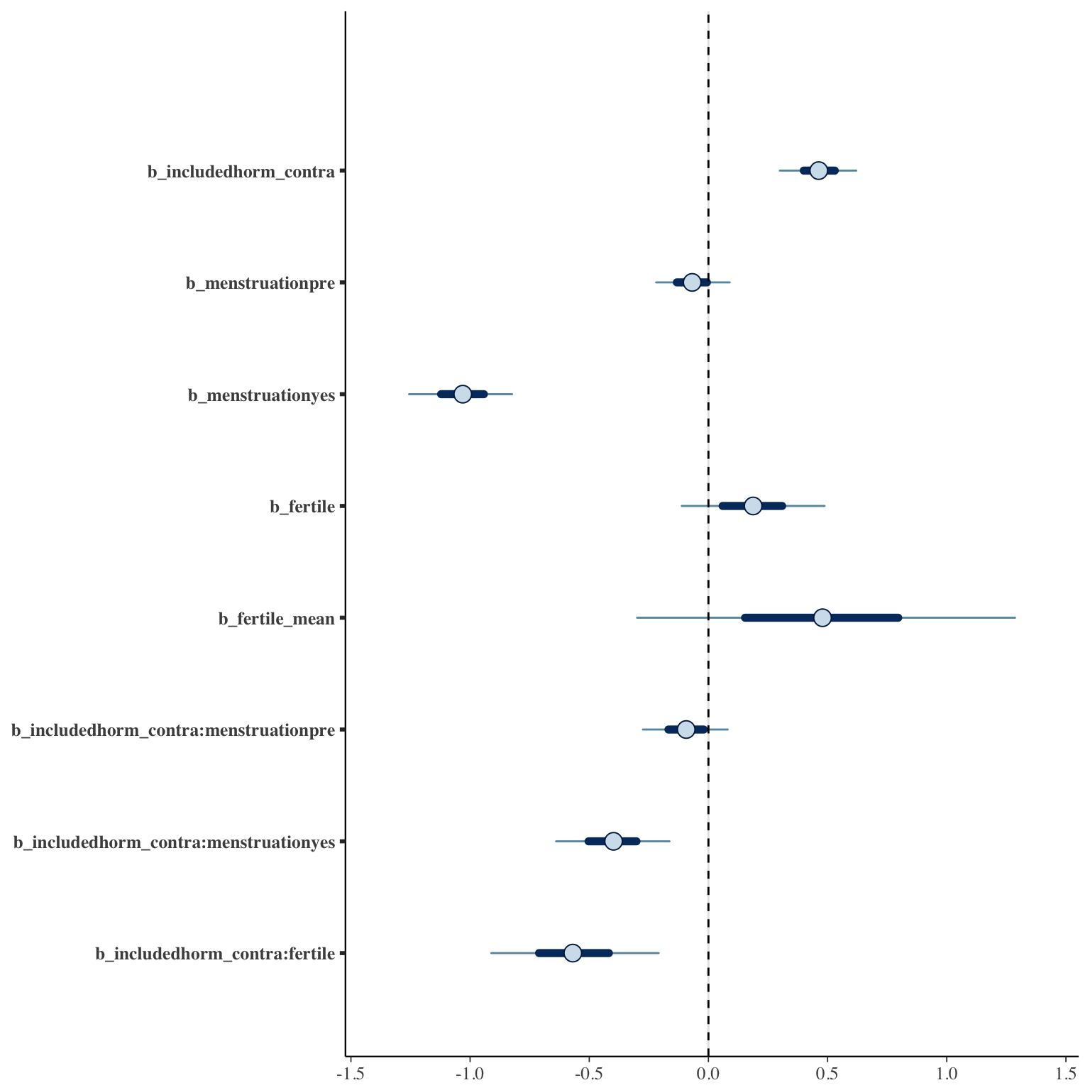
Marginal effect plots
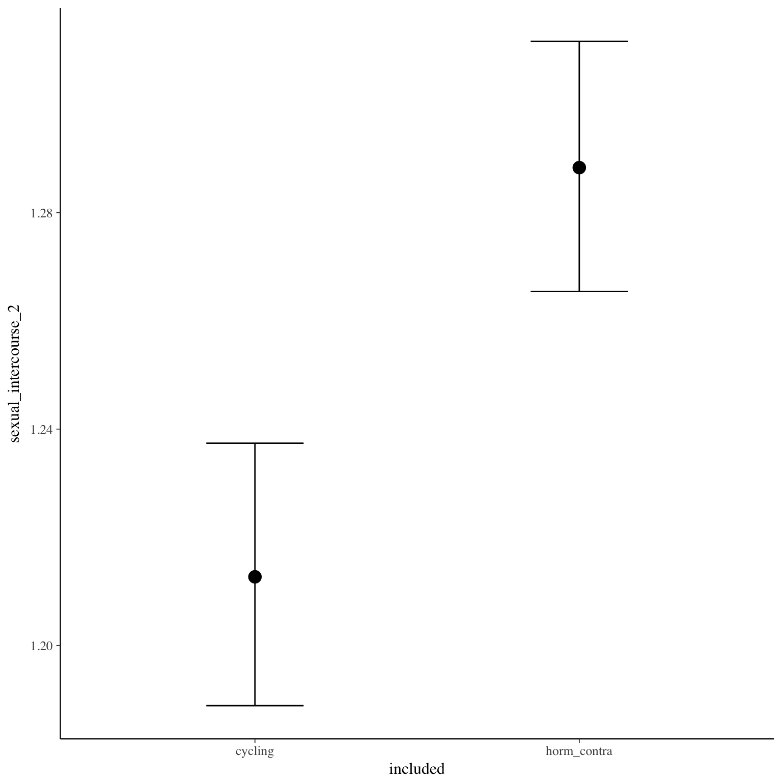
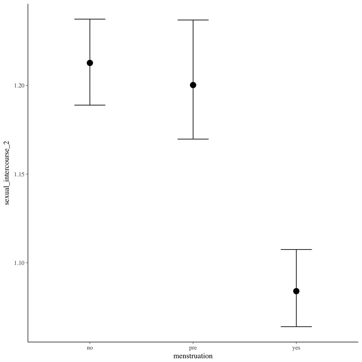
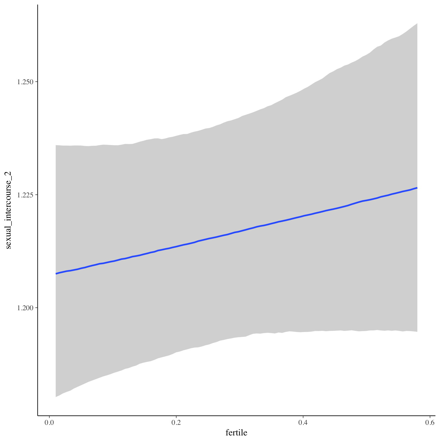
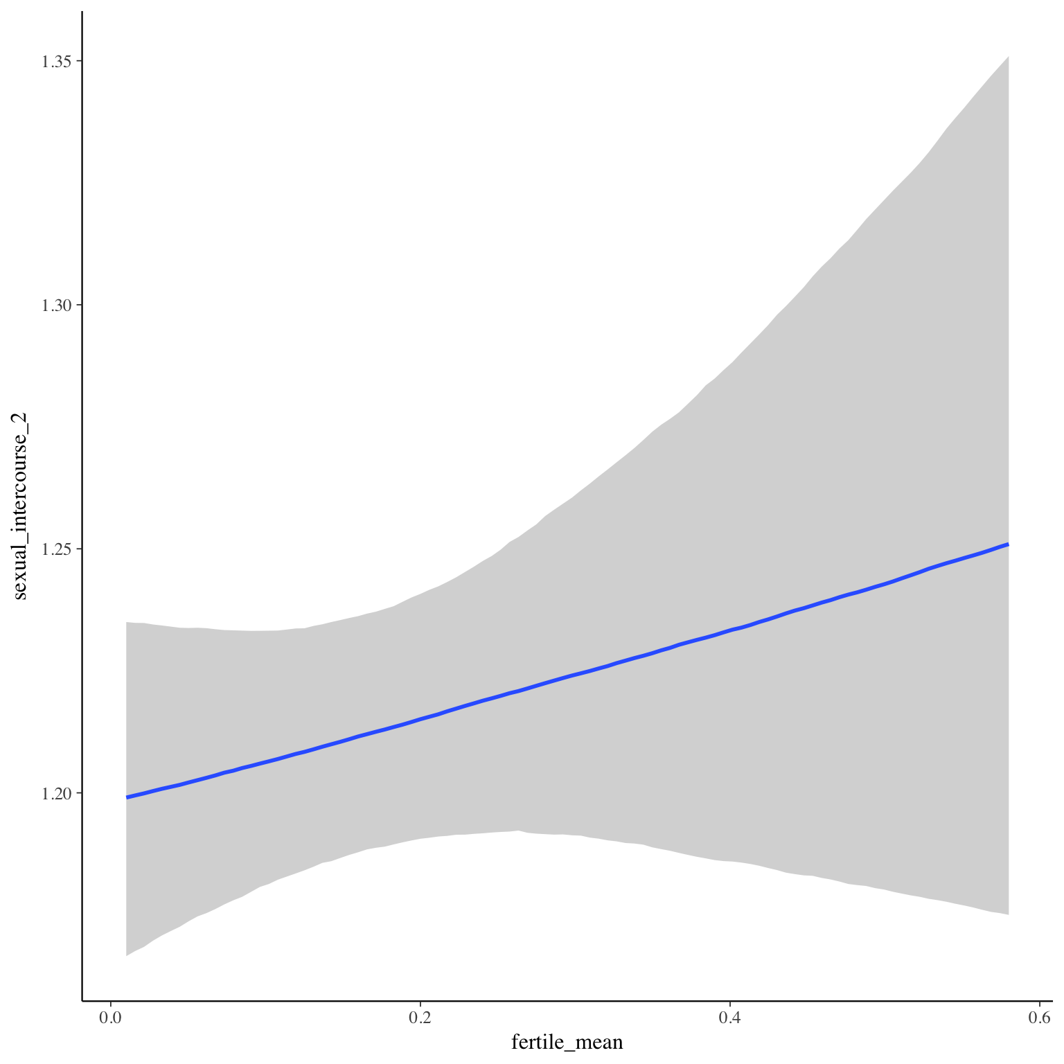
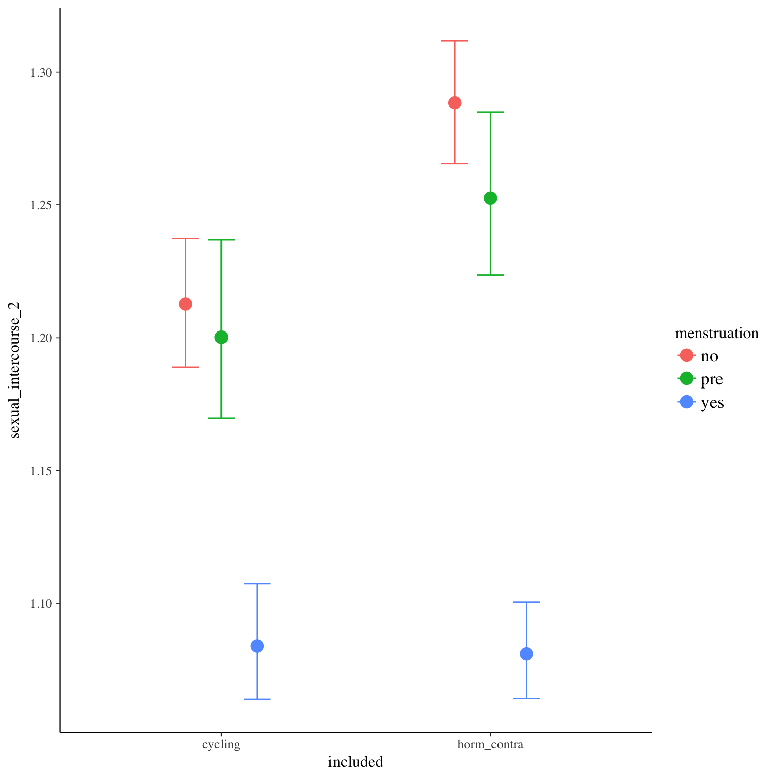
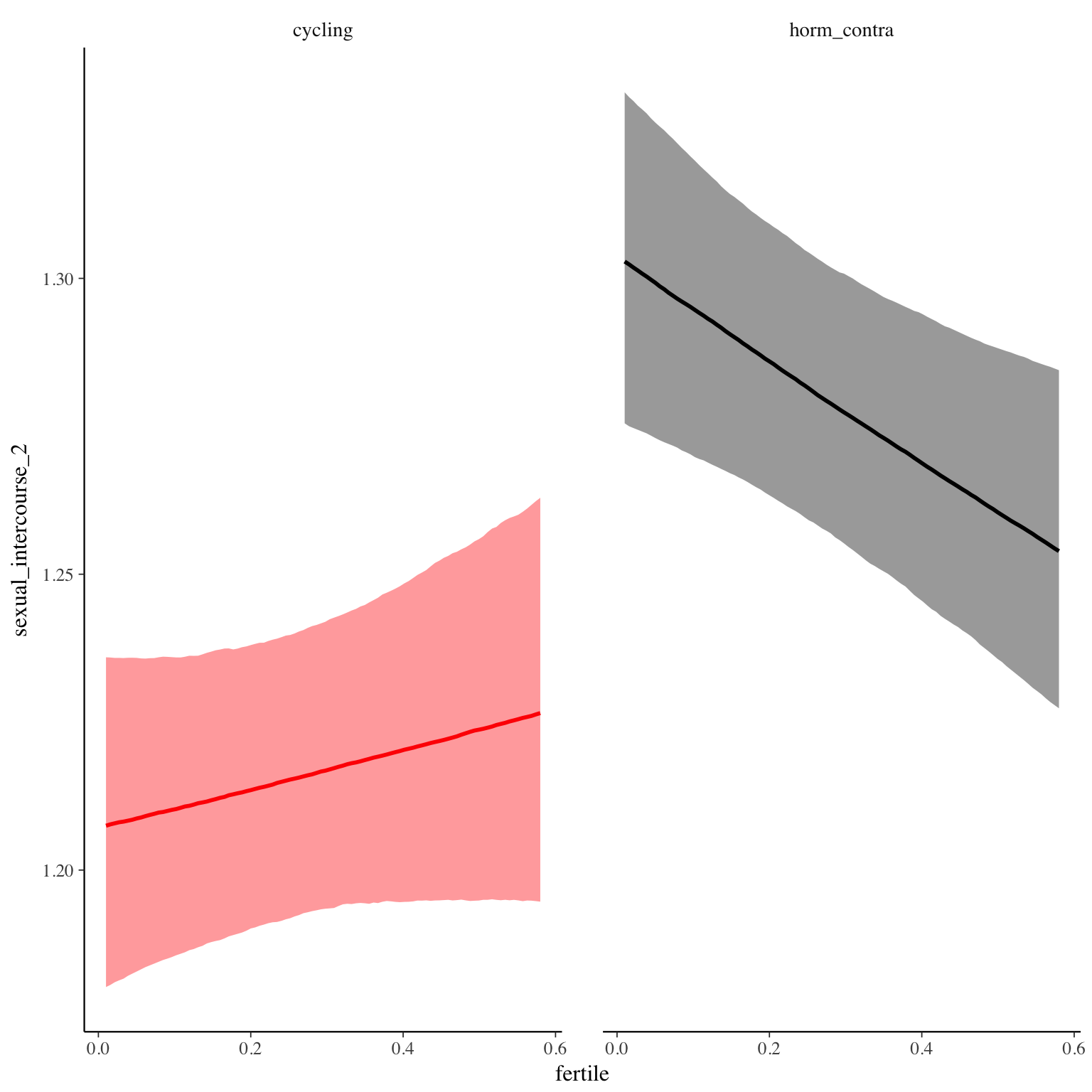
Diagnostics
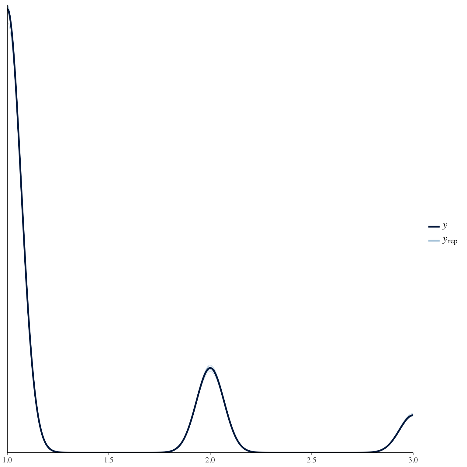
sexual_intercourse_3
Item text:
Wer hat den Geschlechtsverkehr stärker initiiert?
Item translation:
8. Who initiated the sexual intercourse more strongly?
Choices:
| choice | value | frequency | percent |
|---|---|---|---|
| 1 | ich | 2583 | 0.4 |
| 2 | mein Partner | 3929 | 0.6 |
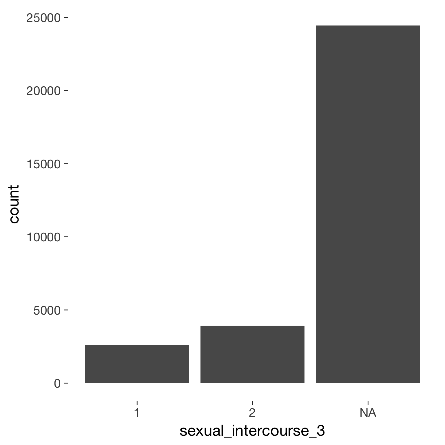
Model
Model summary
 Family: bernoulli(logit)
Formula: sexual_intercourse_3 ~ included * (menstruation + fertile) + fertile_mean + (1 + fertile + menstruation | person)
   Data: diary (Number of observations: 5730)
Samples: 4 chains, each with iter = 2000; warmup = 1000; thin = 1;
         total post-warmup samples = 4000
    ICs: LOO = 7569.73; WAIC = Not computed

Group-Level Effects:
~person (Number of levels: 853)
                                     Estimate Est.Error l-95% CI u-95% CI Eff.Sample Rhat
sd(Intercept)                            0.54      0.08     0.39     0.68        742 1.01
sd(fertile)                              0.57      0.38     0.03     1.38        130 1.01
sd(menstruationpre)                      0.43      0.22     0.04     0.84        275 1.01
sd(menstruationyes)                      0.62      0.26     0.09     1.12        418 1.00
cor(Intercept,fertile)                  -0.13      0.39    -0.79     0.70       1189 1.00
cor(Intercept,menstruationpre)           0.16      0.33    -0.48     0.79        968 1.00
cor(fertile,menstruationpre)            -0.04      0.42    -0.81     0.74        473 1.00
cor(Intercept,menstruationyes)          -0.29      0.29    -0.78     0.39        622 1.01
cor(fertile,menstruationyes)             0.18      0.43    -0.71     0.87        252 1.01
cor(menstruationpre,menstruationyes)    -0.39      0.37    -0.91     0.51        544 1.00

Population-Level Effects:
                                    Estimate Est.Error l-95% CI u-95% CI Eff.Sample Rhat
Intercept                               0.27      0.13     0.02     0.51       1799    1
includedhorm_contra                     0.17      0.11    -0.05     0.39       1418    1
menstruationpre                         0.09      0.15    -0.20     0.40       1662    1
menstruationyes                         0.08      0.17    -0.25     0.42       1800    1
fertile                                -0.38      0.26    -0.92     0.13       1692    1
fertile_mean                            0.77      0.54    -0.24     1.83       3423    1
includedhorm_contra:menstruationpre    -0.19      0.18    -0.56     0.17       1737    1
includedhorm_contra:menstruationyes    -0.54      0.22    -0.97    -0.11       2120    1
includedhorm_contra:fertile             0.45      0.33    -0.20     1.11       1568    1

Samples were drawn using sampling(NUTS). For each parameter, Eff.Sample
is a crude measure of effective sample size, and Rhat is the potential
scale reduction factor on split chains (at convergence, Rhat = 1).
Coefficient plot
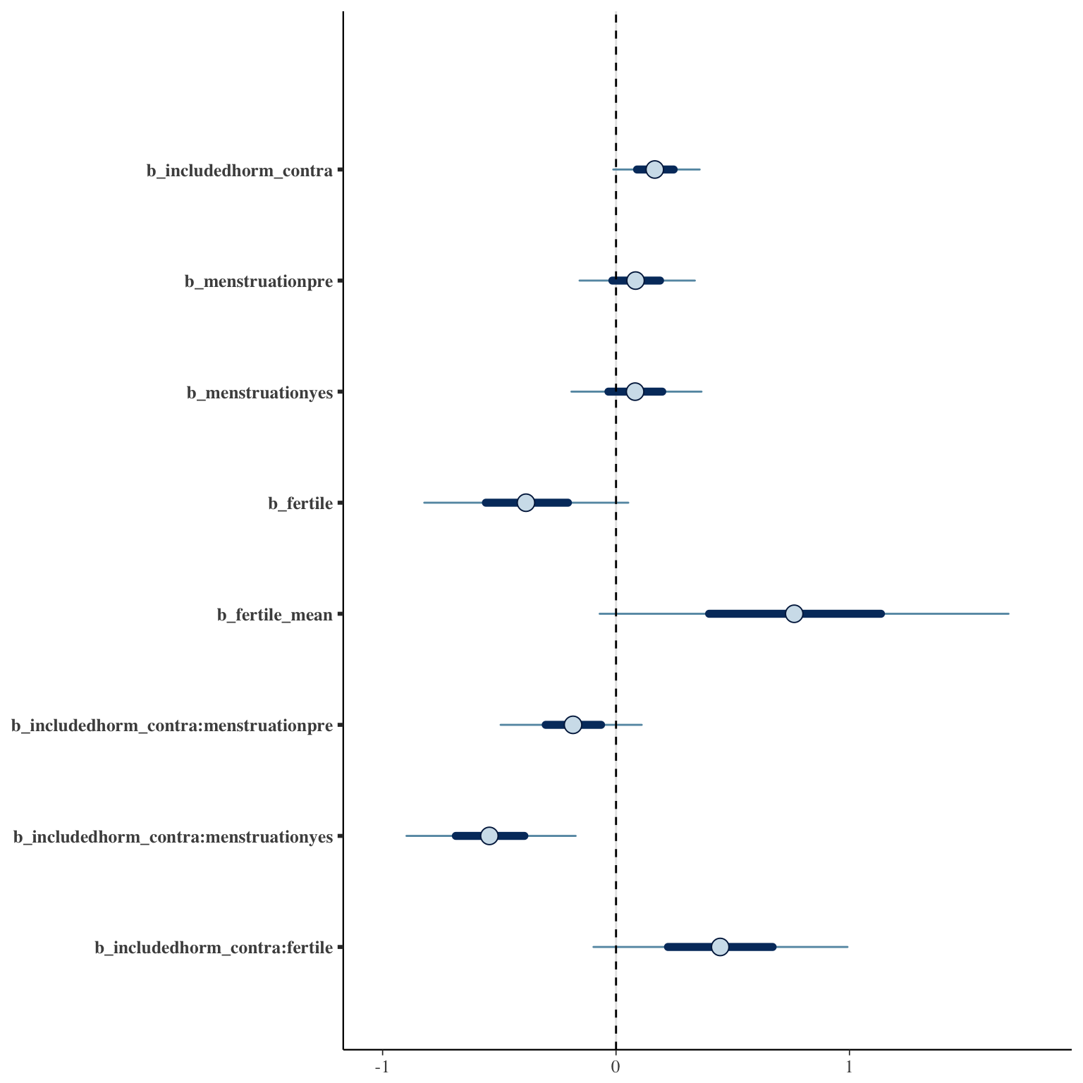
Marginal effect plots

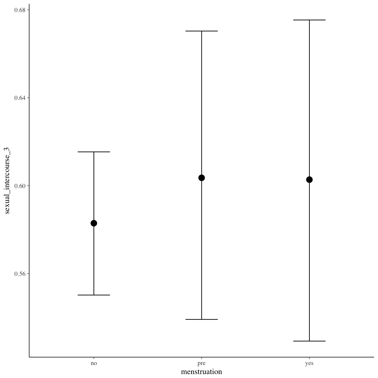
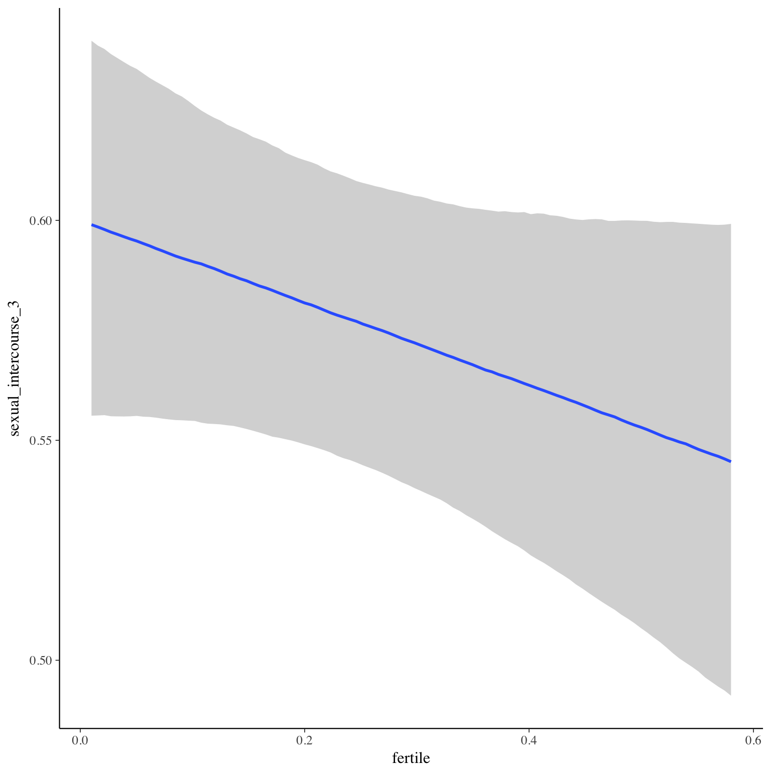
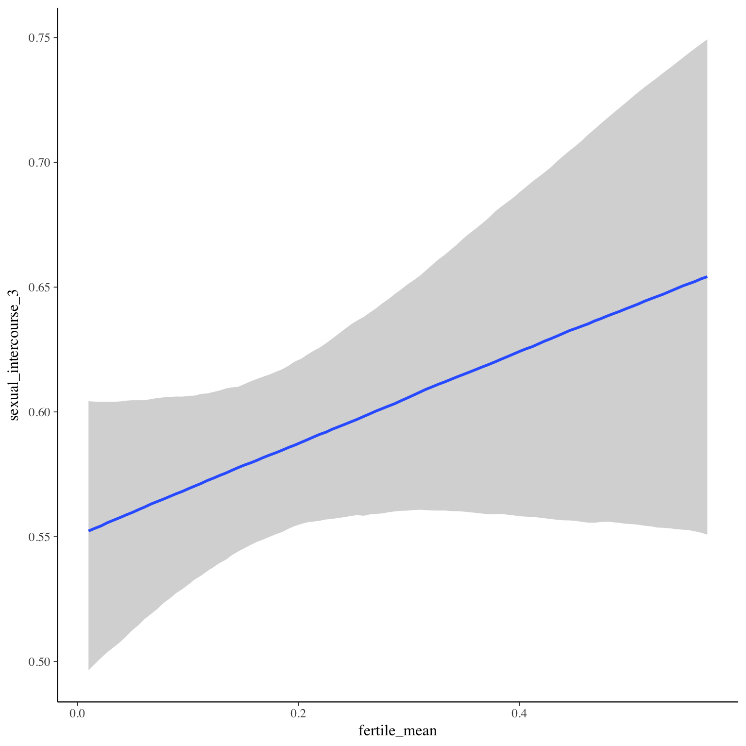
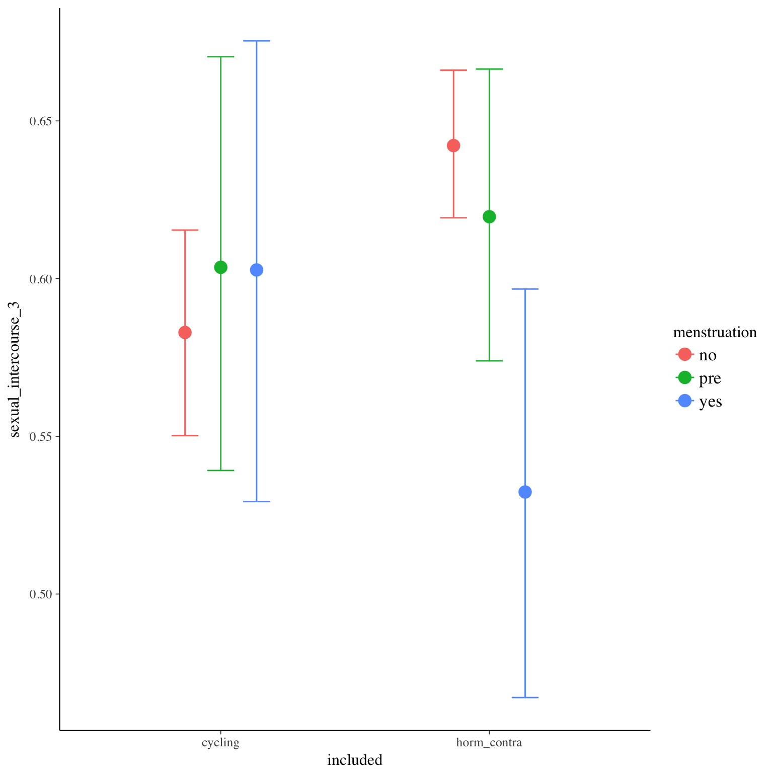
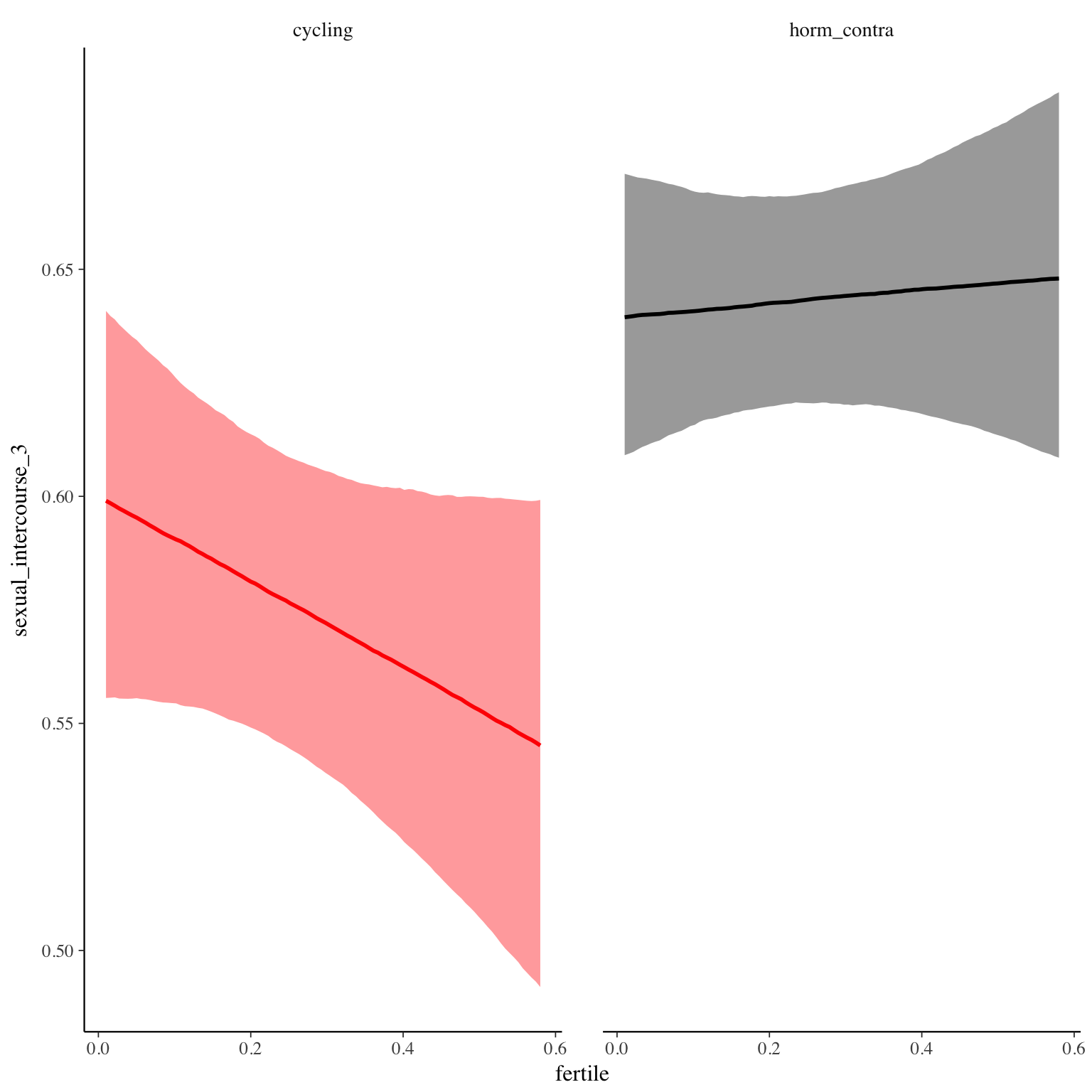
Diagnostics
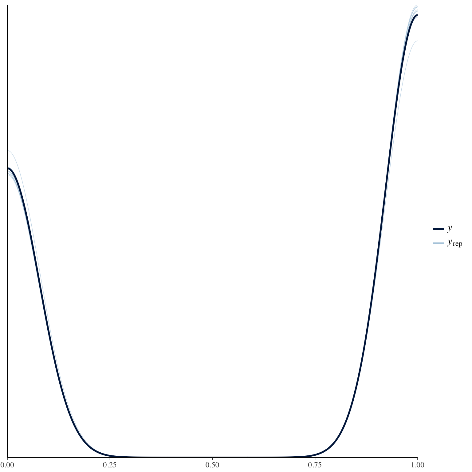
sexual_intercourse_5
Item text:
Hatten Sie seit Ihrem letzten Eintrag anderen sexuellen Kontakt mit Ihrem Partner (Oralverkehr, Petting etc.)?
Item translation:
10. Did you have other forms of sexual contact with your
Choices:
| choice | value | frequency | percent |
|---|---|---|---|
| 0 | NA | 24118 | 0.81 |
| 1 | ja (1x) | 3660 | 0.12 |
| 2 | ja (mehrfach) | 2123 | 0.07 |
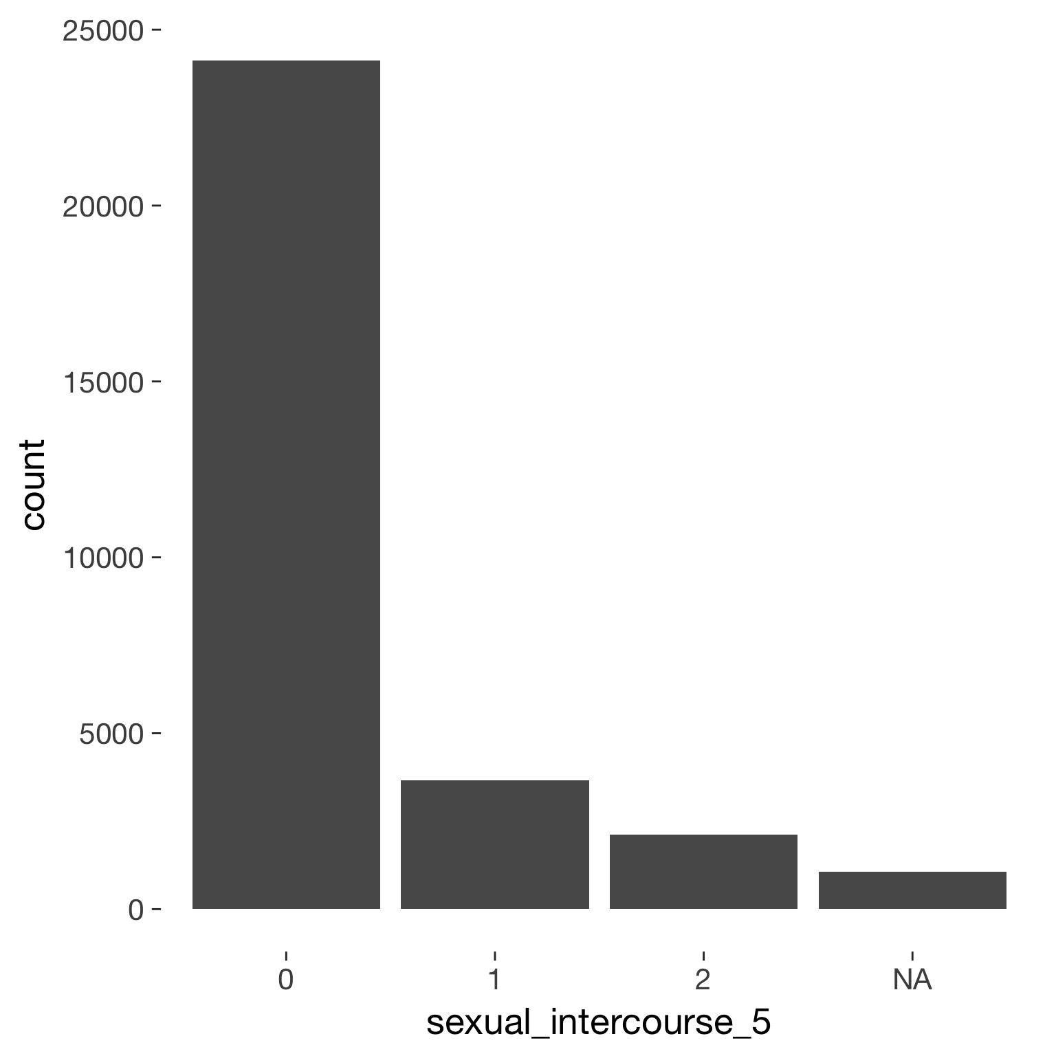
Model
Model summary
 Family: cumulative(logit)
Formula: sexual_intercourse_5 ~ included * (menstruation + fertile) + fertile_mean + (1 + fertile + menstruation | person)
         disc = 1
   Data: diary (Number of observations: 26567)
Samples: 4 chains, each with iter = 2000; warmup = 1000; thin = 1;
         total post-warmup samples = 4000
    ICs: LOO = 29463.19; WAIC = Not computed

Group-Level Effects:
~person (Number of levels: 1043)
                                     Estimate Est.Error l-95% CI u-95% CI Eff.Sample Rhat
sd(Intercept)                            1.17      0.06     1.06     1.28       1268 1.00
sd(fertile)                              1.54      0.18     1.18     1.90        561 1.01
sd(menstruationpre)                      0.67      0.11     0.44     0.87        534 1.01
sd(menstruationyes)                      0.86      0.10     0.68     1.05        801 1.00
cor(Intercept,fertile)                  -0.17      0.10    -0.36     0.05       1426 1.00
cor(Intercept,menstruationpre)          -0.09      0.12    -0.31     0.17       1116 1.00
cor(fertile,menstruationpre)             0.57      0.13     0.28     0.82        468 1.00
cor(Intercept,menstruationyes)          -0.13      0.10    -0.32     0.07        914 1.00
cor(fertile,menstruationyes)             0.05      0.17    -0.30     0.36        326 1.01
cor(menstruationpre,menstruationyes)     0.33      0.16    -0.01     0.62        303 1.01

Population-Level Effects:
                                    Estimate Est.Error l-95% CI u-95% CI Eff.Sample Rhat
Intercept[1]                            1.86      0.12     1.62     2.10       1974    1
Intercept[2]                            3.23      0.12     2.99     3.48       1989    1
includedhorm_contra                     0.34      0.11     0.13     0.56       1412    1
menstruationpre                        -0.19      0.11    -0.41     0.02       1967    1
menstruationyes                        -0.36      0.11    -0.59    -0.13       1930    1
fertile                                 0.09      0.21    -0.33     0.49       2061    1
fertile_mean                           -0.10      0.51    -1.07     0.91       2564    1
includedhorm_contra:menstruationpre     0.02      0.12    -0.21     0.25       2478    1
includedhorm_contra:menstruationyes    -0.07      0.13    -0.32     0.18       2451    1
includedhorm_contra:fertile            -0.46      0.24    -0.92     0.02       2236    1

Samples were drawn using sampling(NUTS). For each parameter, Eff.Sample
is a crude measure of effective sample size, and Rhat is the potential
scale reduction factor on split chains (at convergence, Rhat = 1).
Coefficient plot
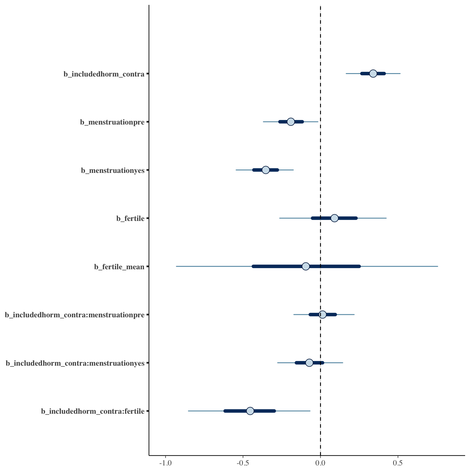
Marginal effect plots
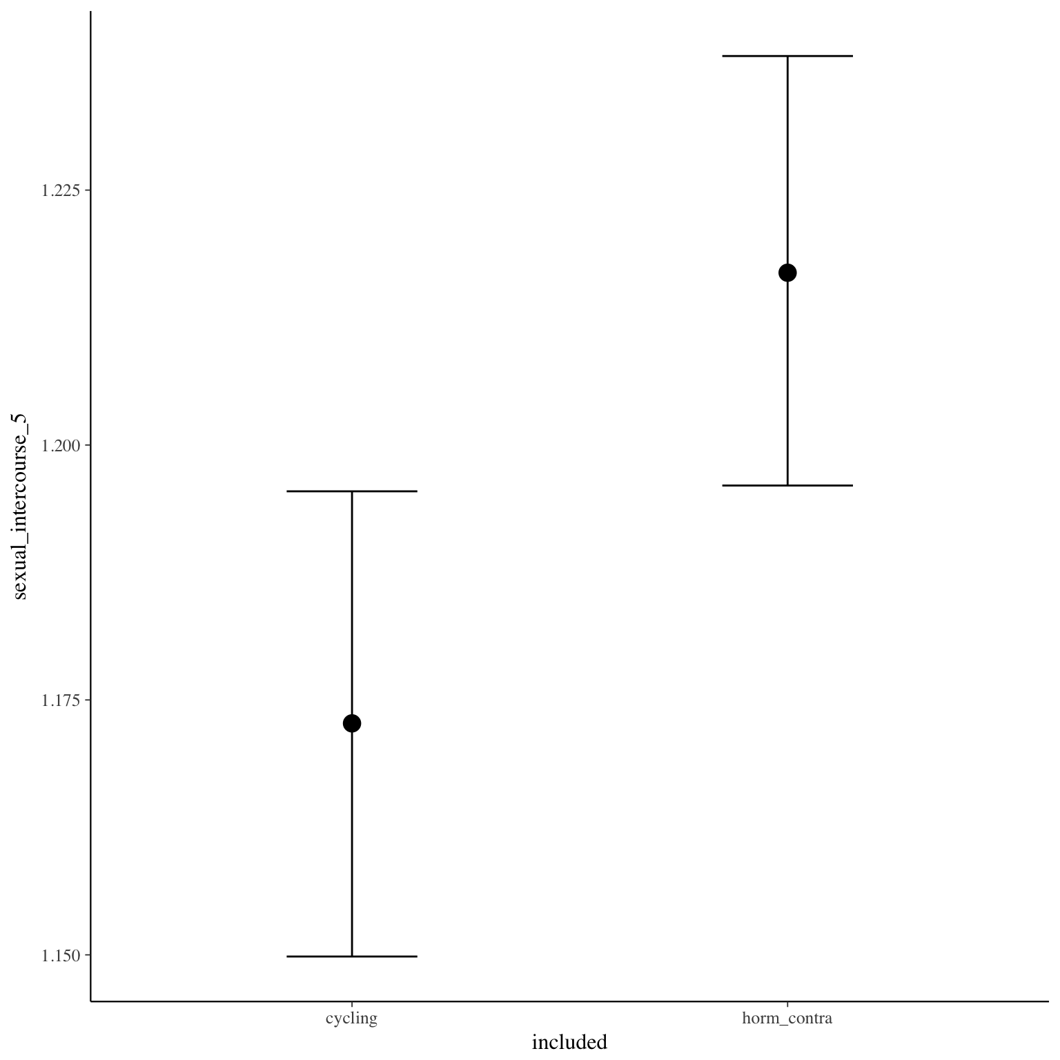
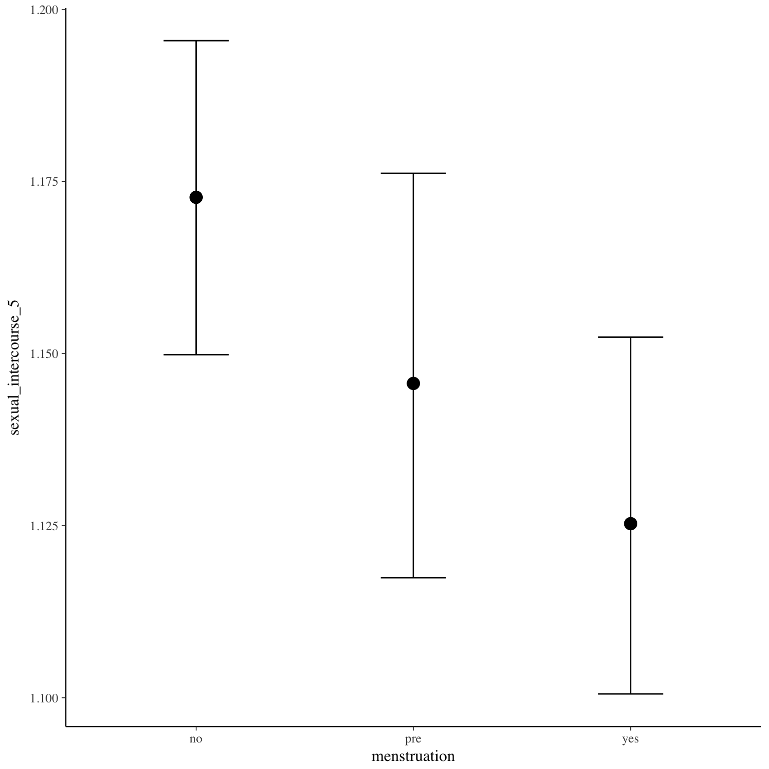
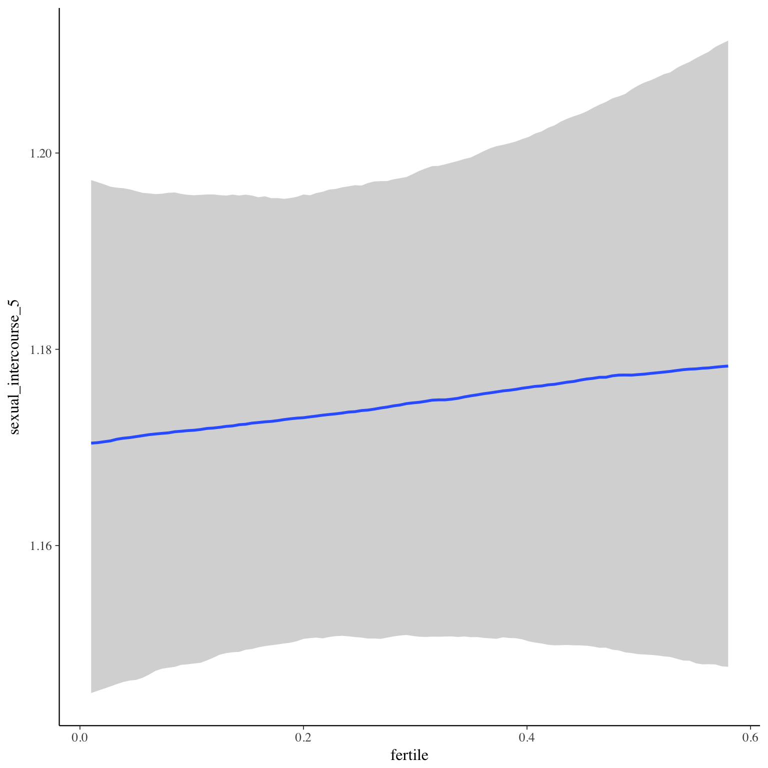
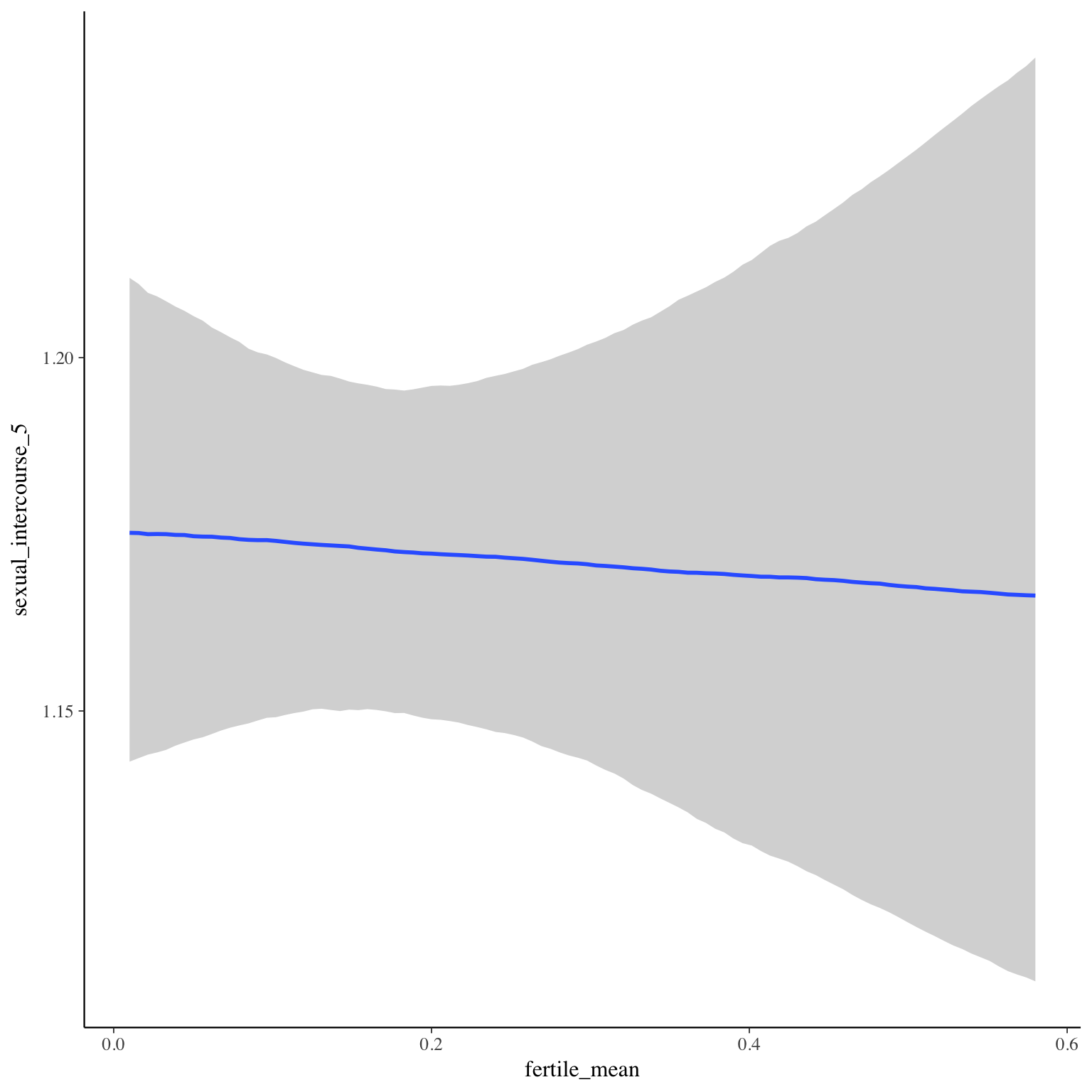
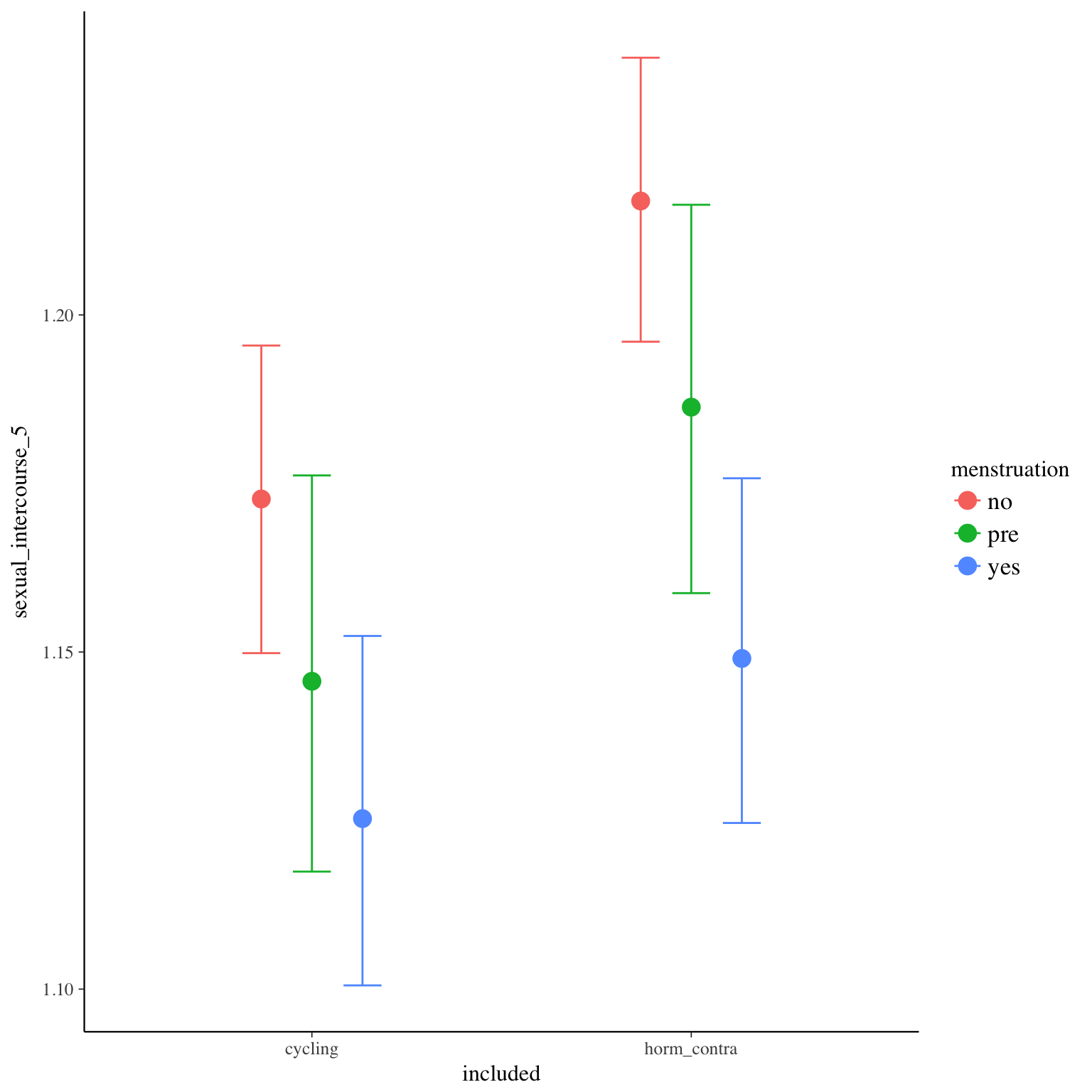
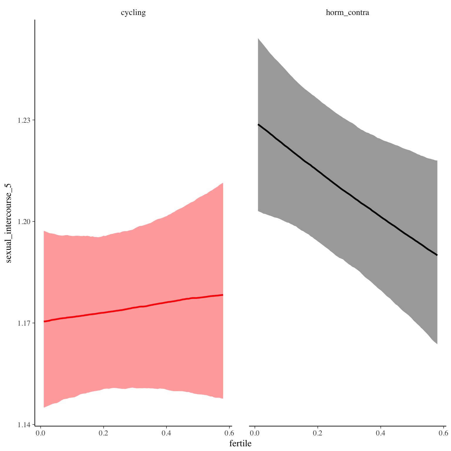
Diagnostics
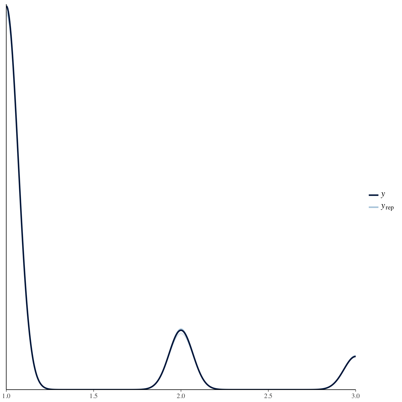
sexual_intercourse_satisfaction
Item text:
Item translation:
Choices:
| choice | value | frequency | percent |
|---|---|---|---|
| 1 | NA | 46 | 0.01 |
| 2 | NA | 78 | 0.01 |
| 3 | NA | 250 | 0.04 |
| 4 | NA | 1361 | 0.21 |
| 5 | NA | 1887 | 0.29 |
| 6 | NA | 2889 | 0.44 |
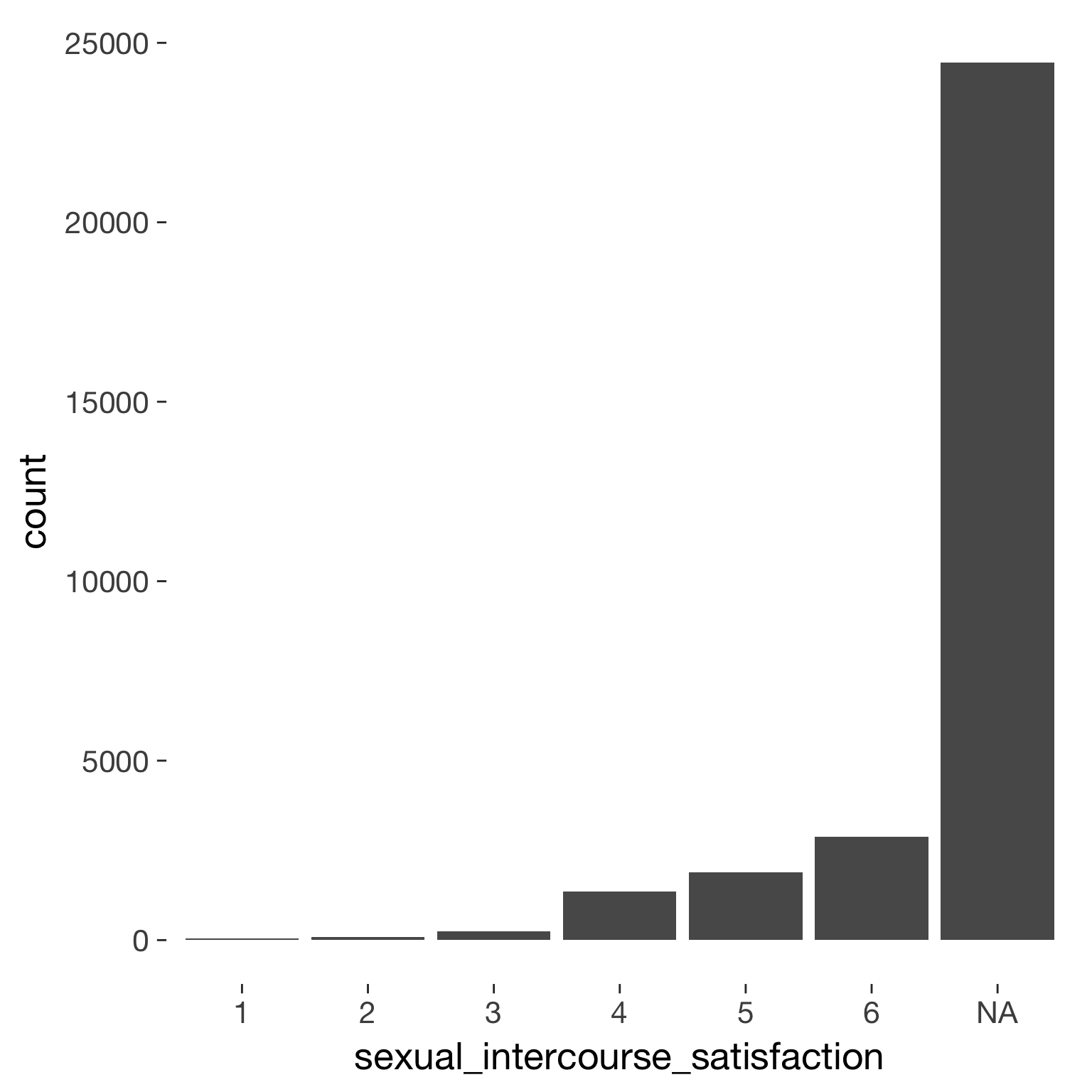
Model
Model summary
 Family: cumulative(logit)
Formula: sexual_intercourse_satisfaction ~ included * (menstruation + fertile) + fertile_mean + (1 + fertile + menstruation | person)
         disc = 1
   Data: diary (Number of observations: 5729)
Samples: 4 chains, each with iter = 2000; warmup = 1000; thin = 1;
         total post-warmup samples = 4000
    ICs: LOO = 12844.77; WAIC = Not computed

Group-Level Effects:
~person (Number of levels: 853)
                                     Estimate Est.Error l-95% CI u-95% CI Eff.Sample Rhat
sd(Intercept)                            1.48      0.08     1.32     1.64       1776 1.00
sd(fertile)                              0.99      0.45     0.10     1.80        176 1.03
sd(menstruationpre)                      0.41      0.20     0.03     0.80        280 1.01
sd(menstruationyes)                      0.97      0.22     0.51     1.37        565 1.02
cor(Intercept,fertile)                  -0.01      0.26    -0.47     0.56       1798 1.00
cor(Intercept,menstruationpre)           0.21      0.28    -0.36     0.72       2170 1.00
cor(fertile,menstruationpre)            -0.03      0.41    -0.80     0.72        470 1.00
cor(Intercept,menstruationyes)          -0.33      0.15    -0.60    -0.01       1350 1.00
cor(fertile,menstruationyes)             0.44      0.32    -0.34     0.90        290 1.01
cor(menstruationpre,menstruationyes)    -0.45      0.35    -0.92     0.36        331 1.02

Population-Level Effects:
                                    Estimate Est.Error l-95% CI u-95% CI Eff.Sample Rhat
Intercept[1]                           -6.07      0.24    -6.56    -5.61       4000    1
Intercept[2]                           -4.89      0.20    -5.29    -4.50       4000    1
Intercept[3]                           -3.57      0.18    -3.92    -3.21       3324    1
Intercept[4]                           -1.29      0.17    -1.63    -0.96       3454    1
Intercept[5]                            0.39      0.17     0.05     0.72       3492    1
includedhorm_contra                     0.10      0.15    -0.19     0.39       2571    1
menstruationpre                        -0.04      0.14    -0.32     0.24       4000    1
menstruationyes                        -0.11      0.18    -0.45     0.24       4000    1
fertile                                 0.19      0.28    -0.37     0.75       4000    1
fertile_mean                           -0.21      0.71    -1.60     1.20       4000    1
includedhorm_contra:menstruationpre     0.11      0.18    -0.23     0.46       4000    1
includedhorm_contra:menstruationyes    -0.04      0.23    -0.48     0.40       4000    1
includedhorm_contra:fertile            -0.54      0.34    -1.21     0.13       4000    1

Samples were drawn using sampling(NUTS). For each parameter, Eff.Sample
is a crude measure of effective sample size, and Rhat is the potential
scale reduction factor on split chains (at convergence, Rhat = 1).
Coefficient plot
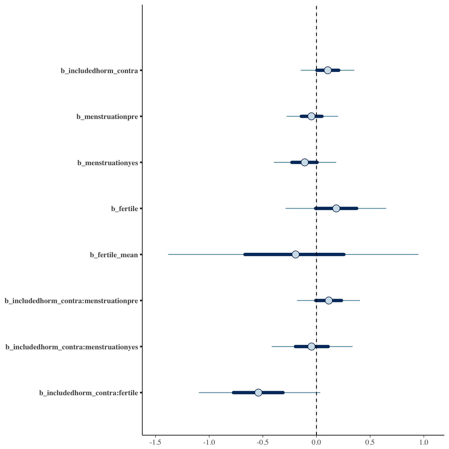
Marginal effect plots
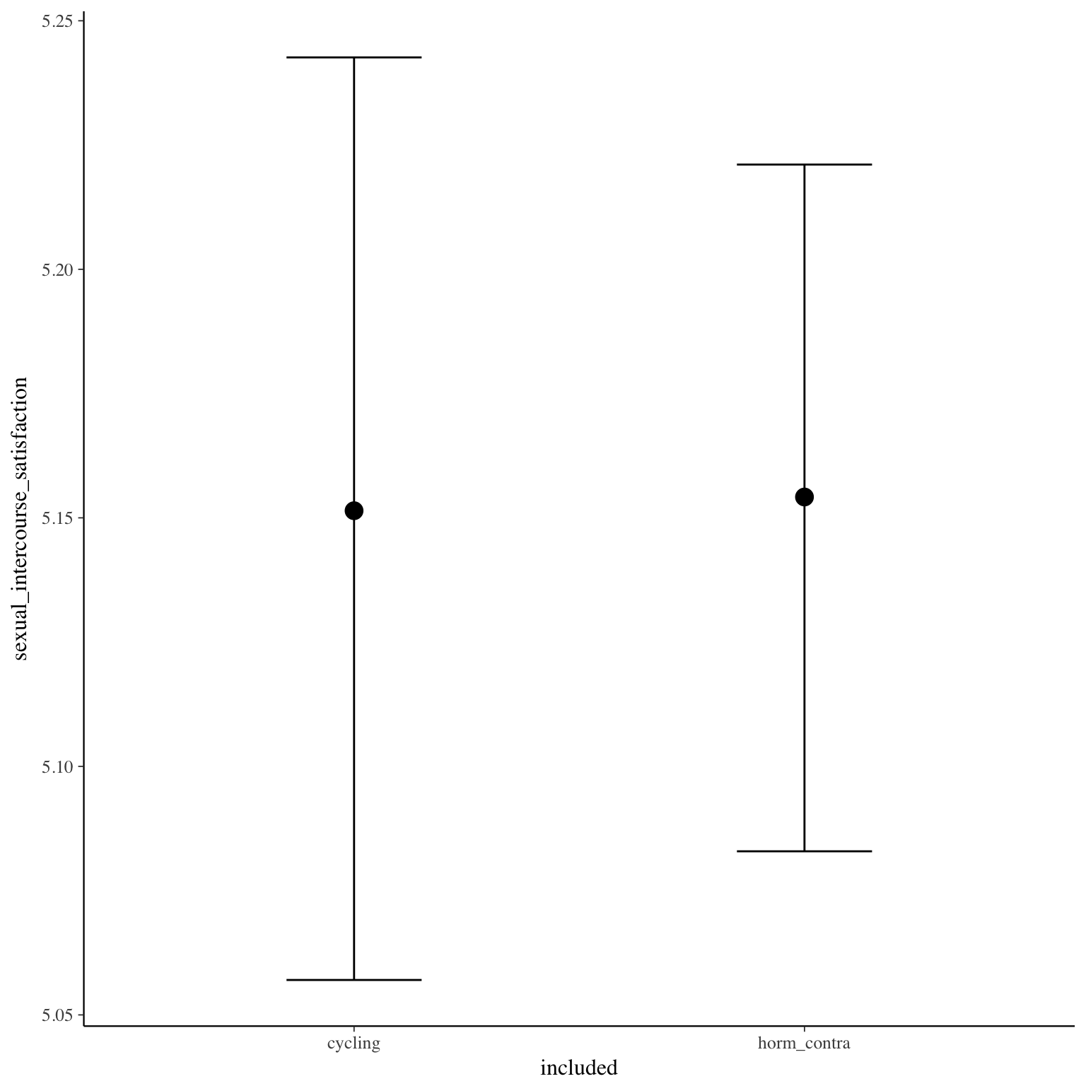
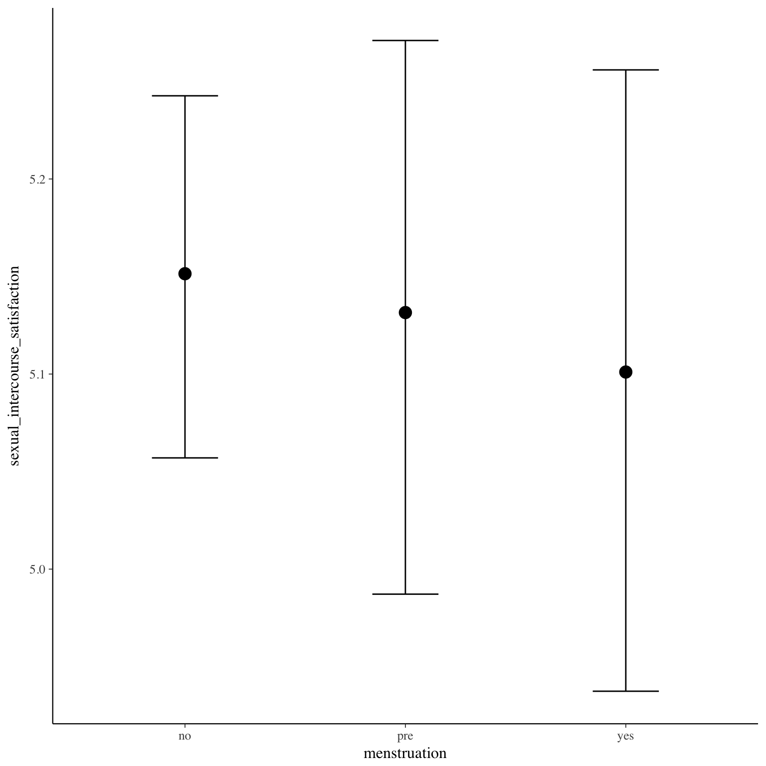
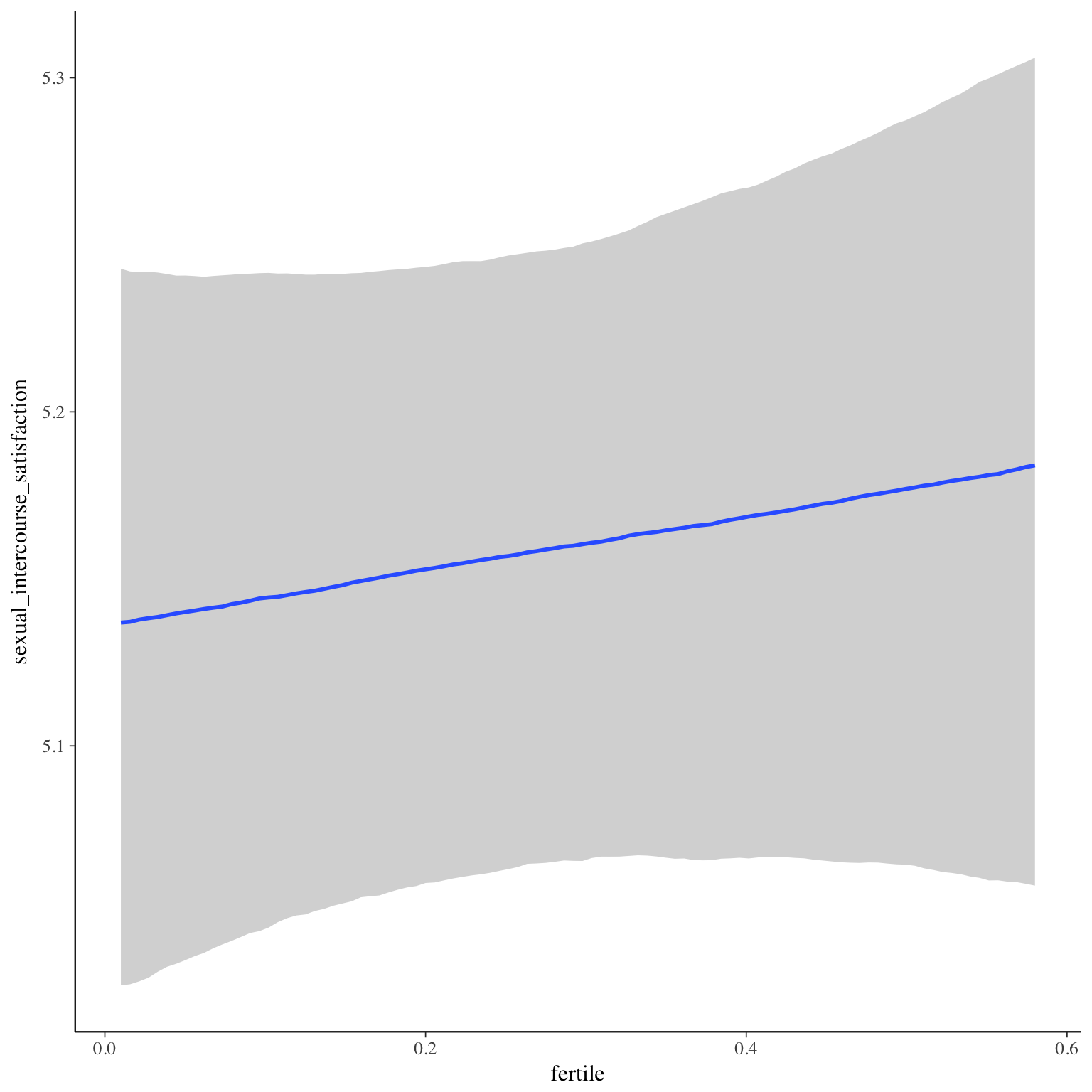
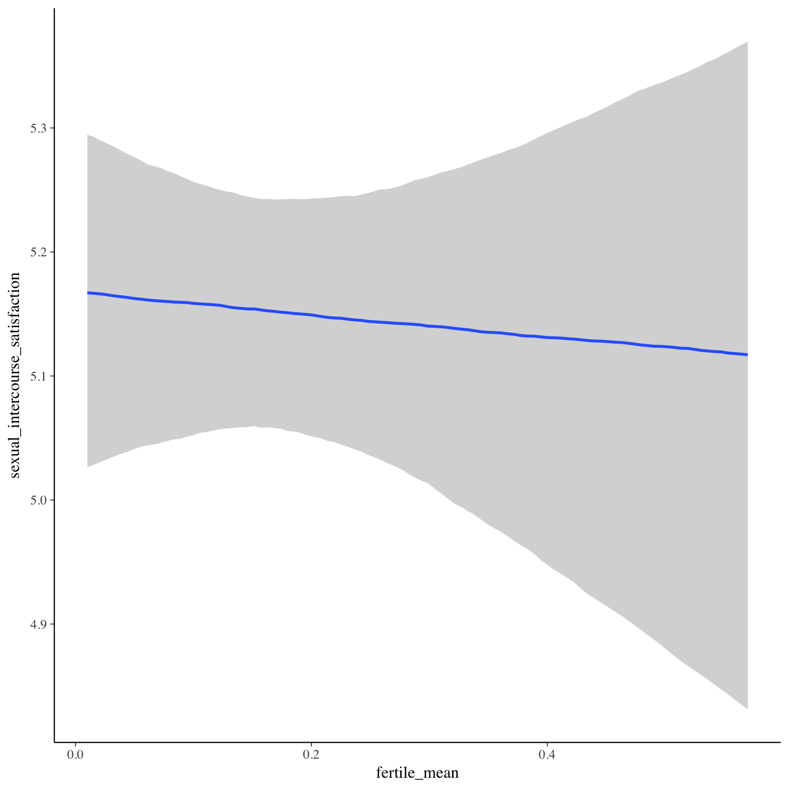
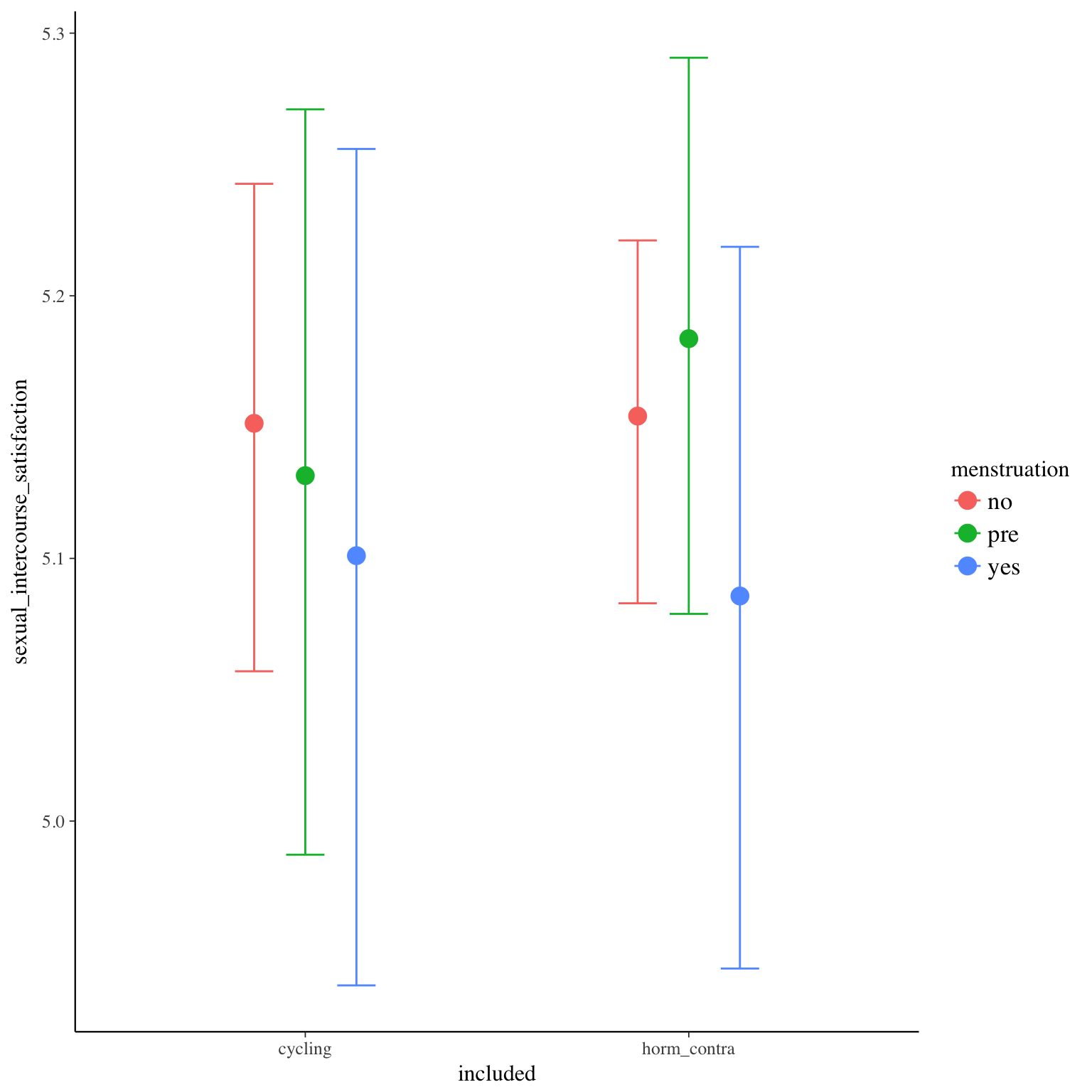
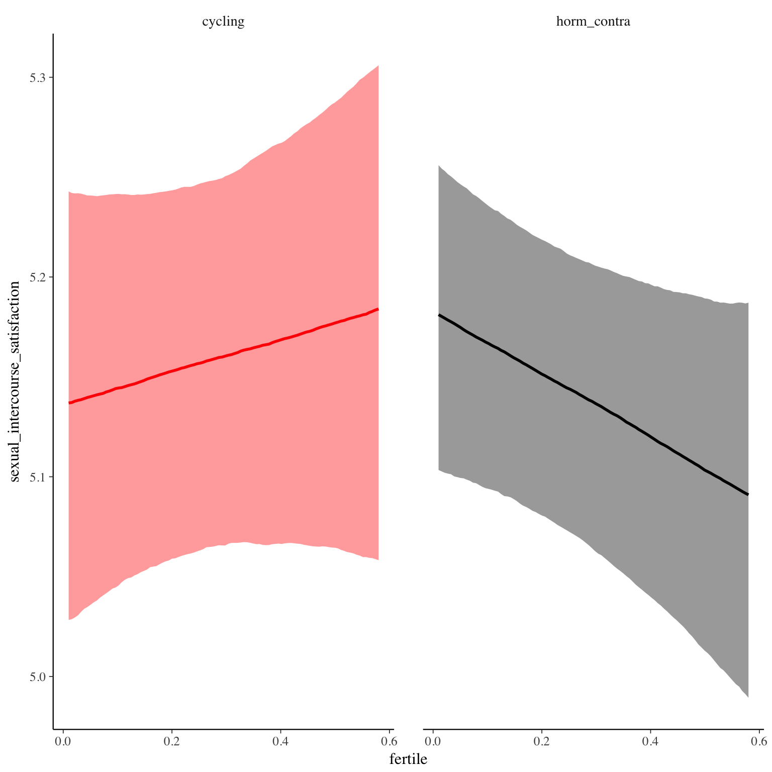
Diagnostics
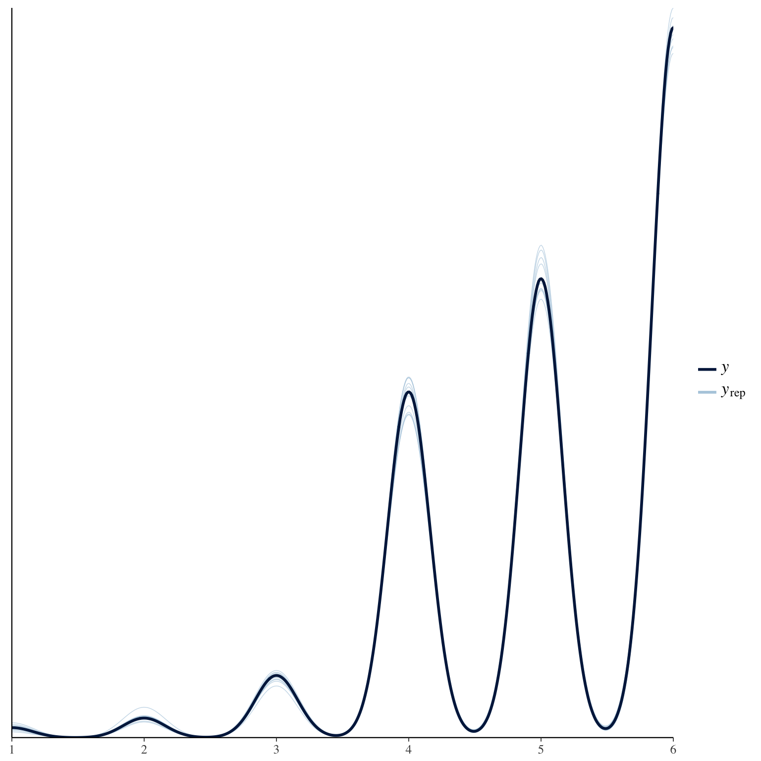
All models
Coefficient plot
coefs = bind_rows(fertile_eff_by_item)
coefs = coefs  %>%
  mutate(contraception = ifelse(term == "fertile", "cycling", "hormonally\ncontracepting")) %>%
  group_by(outcome) %>%
  mutate(fertmean = na.omit(ifelse(term == "fertile", mean, NA_real_))) %>%
  ungroup() %>%
  arrange(desc(fertmean), outcome)


coefs  %>%
  mutate(outcome = factor(outcome, levels = coefs$outcome %>% unique() %>% rev()))  %>%
ggplot(., aes(x = outcome, y = mean, ymin = X2.5., ymax = X97.5., color = contraception)) +
  geom_linerange(aes(ymin = X20., ymax = X80.), position = position_dodge(width = 0.2), size = 1.5) +
  geom_linerange(aes(ymin = X10., ymax = X90.), position = position_dodge(width = 0.2), size = 1) +
  geom_linerange(position = position_dodge(width = 0.2), size = 0.5) +
  geom_linerange(aes(ymin = X0.5., ymax = X99.5.), position = position_dodge(width = 0.2), size = 0.3) +
  geom_point(position = position_dodge(width = 0.2), size = 3) +
  scale_color_manual("", values = c("hormonally\ncontracepting" = "black","cycling" = "red"), guide = F) +
  ylab("regression slope") +
  geom_hline(yintercept = 0, linetype = 'dashed') +
  coord_flip()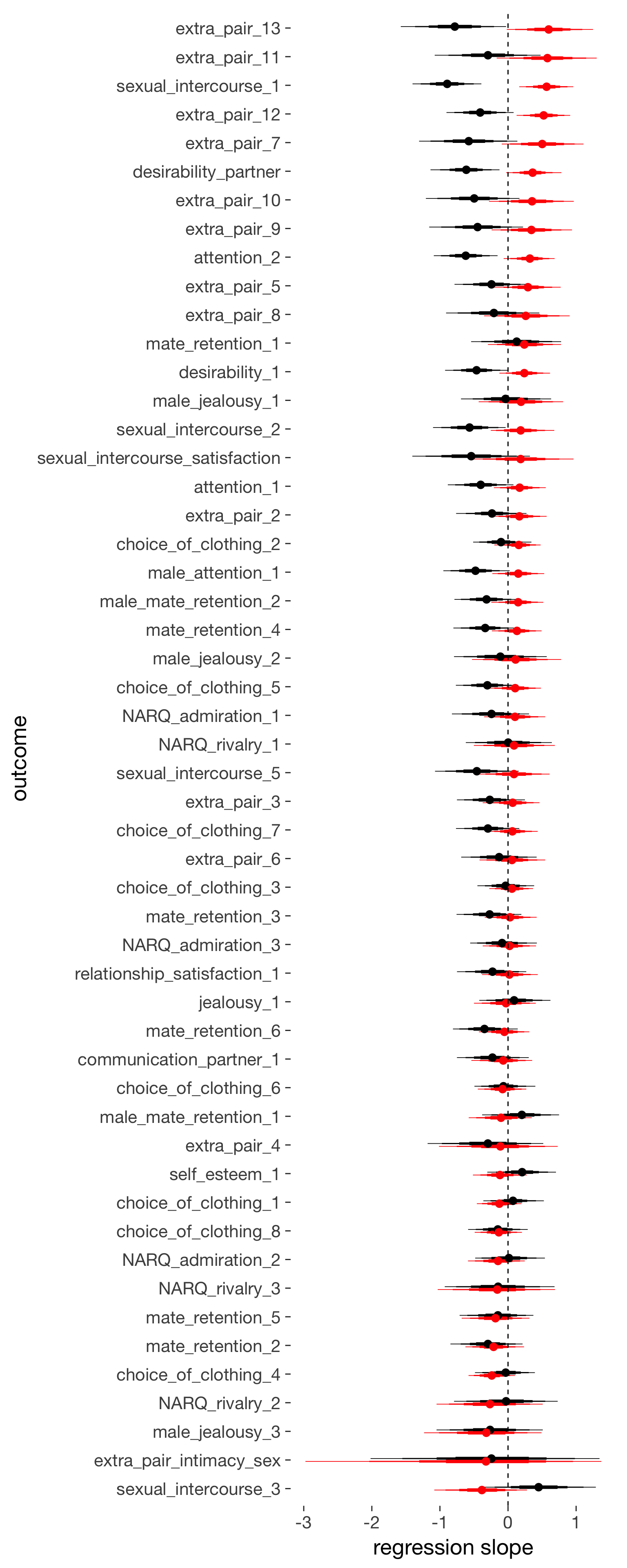
Table
library(DT)
coefs %>%
  mutate(
        mean = form(mean),
        `95% CI` = paste0("[", form(X2.5.,2) , ";", form(X97.5.,2) , "]"),
         label = paste0(label, " [", outcome, "]")) %>%
  select(label, contraception, mean, `95% CI`) %>%
  datatable(rownames = FALSE, filter = "top", extensions = 'Buttons', options = list(
    dom = 'Bfrtip',
    buttons = c('copy', 'csv', 'excel', 'pdf', 'print'),
    pagelength = 40
  ))